solving hydrogen atom problem using spherical …
TRANSCRIPT
European J of Physics Education Volume 10 Issue 4 1309-7202 Singh
1
SOLVING HYDROGEN ATOM PROBLEM USING SPHERICAL POLAR
COORDINATES: A QUALITATIVE STUDY
Satya Pal Singh
AS-205, Computational Condensed Matter Physics Laboratory Department of Applied Sciences
Madan Mohan Malaviya University of Technology Gorakhur-273010, (UP) India [email protected]
(Received 20.06.2019, Accepted 24.08.2019)
Abstract
Quantum mechanics has completed century since its genesis. Quantum mechanics is taught at various levels-starting from school and colleges to universities. Regression methods are introduced at under graduate and post graduate levels to solve Schrodinger equation for finding solutions of various trivial and non-trivial physical problems. The common problems, which students encounter at UG level are- particle in a box, potential step and barriers, harmonic oscillator and hydrogen atom. It has been observed that students lack clarity in solving and grasping the hydrogen atom problem. Two reasons can be accounted for this. It is perhaps a lengthy derivation and students, many times, are not well acquainted with the requisite knowledge of Spherical Polar Co-ordinate system. In this article, a brief review on the birth of quantum mechanics is presented judiciously discussing the contribution of Schrodinger, before solving the hydrogen atom problem. Readers are first introduced to spherical-polar coordinate system. The radial solutions, radial probability distribution functions, and hydrogen orbital, are plotted using Mathematica software v.12, for the sake of visualization and understanding .
INTRODUCTION
The spectra of many elements have been known, since 19th century. The emission and absorption of different, but of definite wavelengths (i.e. color) radiations, work like a fingerprint to recognize chemical elements. In other words, the spectra of atoms are signatures of the electronic distribution inside atoms. But the emission and absorption of radiation, in visible spectra, had remained a mystery for a century, until Planck gave the idea of quanta and proposed that light travels in form of quanta. Quantum mechanics was born in the year 1900, when Max Planck derived a formula for black body radiation in order to explain it, for all possible wavelengths (Alain& Villain, 2017). Planck introduced the concept of quantization of energy. He proposed that radiation travels in form of quanta (i.e. a bundle of energy). In 1905, Einstein introduced the

European J of Physics Education Volume 10 Issue 4 1309-7202 Singh
2
notion of “Lichtquanten” (i.e. quantum of light). Twenty years later, it was named photon. He realized the importance of the idea of quantization to explain photoelectric effect. In the year 1905, also rendered as miraculous year in the history of science, Einstein published three historical papers; one dealing with special relativity, another with Brownian motion and the third one with photoelectric effect. He used quantum nature of light to explain photoelectric effect. Wave nature of light could already explain optical phenomena as interference, diffraction and polarization.
In 1913, the ground breaking discovery of Bohr atomic model further extended the idea of quantization, because Bohr postulated that electrons in atoms can move only in definite orbits, and it can emit or absorb radiation in form of definite quanta only. The experimental observation of hydrogen atom spectra Figure (1) was already reported by contemporary scientists. But, no satisfactory theory existed, which could explain it.These developments led Louis de Broglie to propose the idea of wave-particle duality in 1923, as a part of his doctoral dissertation. He wanted to introduce the idea of “Atom of Light”, but his principal examiner Paul Lanevin consulted Einstein regarding this. Einstein, appreciated the idea of wave-particle duality, but could not agree with the idea of atom of light. Broglie removed the latter part and obtained his Ph.D degree.Broglie re-derived Bohr’s quantization rules (Alain& Villain, 2017).
Figure 1.Absorption and emission lines in hydrogen atom spectra (H-α lines are most intense)
It had become quite natural for the contemporary physicists to raise question about the wave equation; that could be solved to obtain such solutions. In 1926, Schrodinger Figure (2) solved problems in a series of papers. In a co-parallel manner, Heisenberg (Heisenberg, 1925) Born and Jordan (Born & Jordan, 1925) published their matrix version of quantum mechanics in 1925 (Aschman & Keaney, 1989; Reiter &Yngvason, 2013; Fedak & Jeffrey 2009). Modern quantum mechanics was born, when Schrodinger demonstrated equivalence with their matrix formalism by exactly solving the hydrogen atom problem and explain it’s spectra.

European J of Physics Education Volume 10 Issue 4 1309-7202 Singh
3
Figure 2. Left: Erwin Schrodinger (1887-1961) (Courtesy: R. Braunizer 1926); Right: Tomb of
Schrodinger and his wife with plaque imprinted with his famous equation (Courtesy: C. Joas 2008)
A relativistic version of his equation came within a year. Klein, Gordon and Fock gave relativistic equation for a free particle. The relativistic treatment of hydrogen atom was introduced by P. A. M. Dirac in 1928.Opposite to matrix calculus of Heisenberg, Schrodinger’s approach is quite simple. Schrodinger equation can be derived considering spatial distribution of the amplitude of the wave ψ(x), at a fixed point in time as follows-
( ) + ( ) = 0; 푘 = &휆 = ℎ/푝 (1)
( ) + ( ) = 0; 푝 = 2푚(퐸 − 푉) (2)
( ) + ( ) ( ) = 0 (3)
The premises of quantum mechanics have gotten developed tremendously, since its birth
in the beginning of 20th century. Almost every walk of science needs it, especially when the problem is rooted at the bottom of the scale. From nanoscience to cosmology, its knowledge has become mandatory in order to fully narrate natures beauty in terms of mathematical formalism. Here, the exact solution of hydrogen atom, using Schrodinger equation is obtained in a greater detail in a pedagogical manner. MATHEMATICAL ANALYSIS Though, hydrogen atom problem has become a century old problem and numerous text books (Ghatak & Loknathan, 2004; Schiff & Bandhyopadhyay, 2017) (Feynman, 2015) and documents
European J of Physics Education Volume 10 Issue 4 1309-7202 Singh
4
are available to solve it including online references (Chapter-10 The Hydrogen Atom) we shall start with a fresh cumulative approach. We shall first convert three-dimensional Schrodinger equation from Cartesian coordinate system to spherical coordinate system.
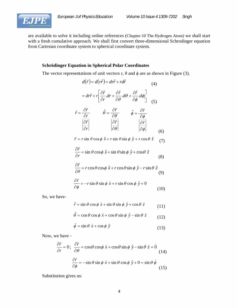
Schrödinger Equation in Spherical Polar Coordinates
The vector representations of unit vectors r, θ and ϕ are as shown in Figure (3).
rrdrdrrrdrd ˆˆˆ
(4)
drdrdrrrrrdr .
ˆ.
ˆ.
ˆˆ (5)
rrrrr
ˆ
r
rˆ
r
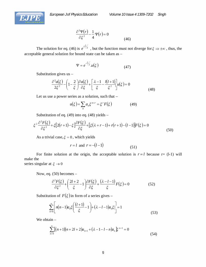
rˆ
(6)
zryθrxθrr ˆ cosˆ sinsinˆ cossin (7)
zyθxθrr ˆ cosˆ sinsinˆ cossin
(8)
zryθrxθrθr ˆ sinˆ sincosˆ coscos
(9)
0ˆ cossin sinsin yrxrr
(10)
So, we have- zyxr cosˆ sinsin cossinˆ (11)
zyx sinˆ sincos coscosˆ (12)
yx ˆ cos sin (13)
Now, we have -
0
rr ; 0 sinˆ sincos coscos
zyxr
(14)
sin0ˆ cossin sinsin yxr
(15)
Substitution gives us:
European J of Physics Education Volume 10 Issue 4 1309-7202 Singh
5
sin drrdrdrrd (16)
fdfrdrr (17)
rdfdfdr
frdrffd
....
(18)
sin . .. 0 drfdrfrdrfrdrf (19)
f
rff
rf
rffr .
sin1..1
(20)
sin11
rrrrr
(21)
2
2
222
22
sin1sin
sin11.
f
rf
rf
rr
rrf
(22)
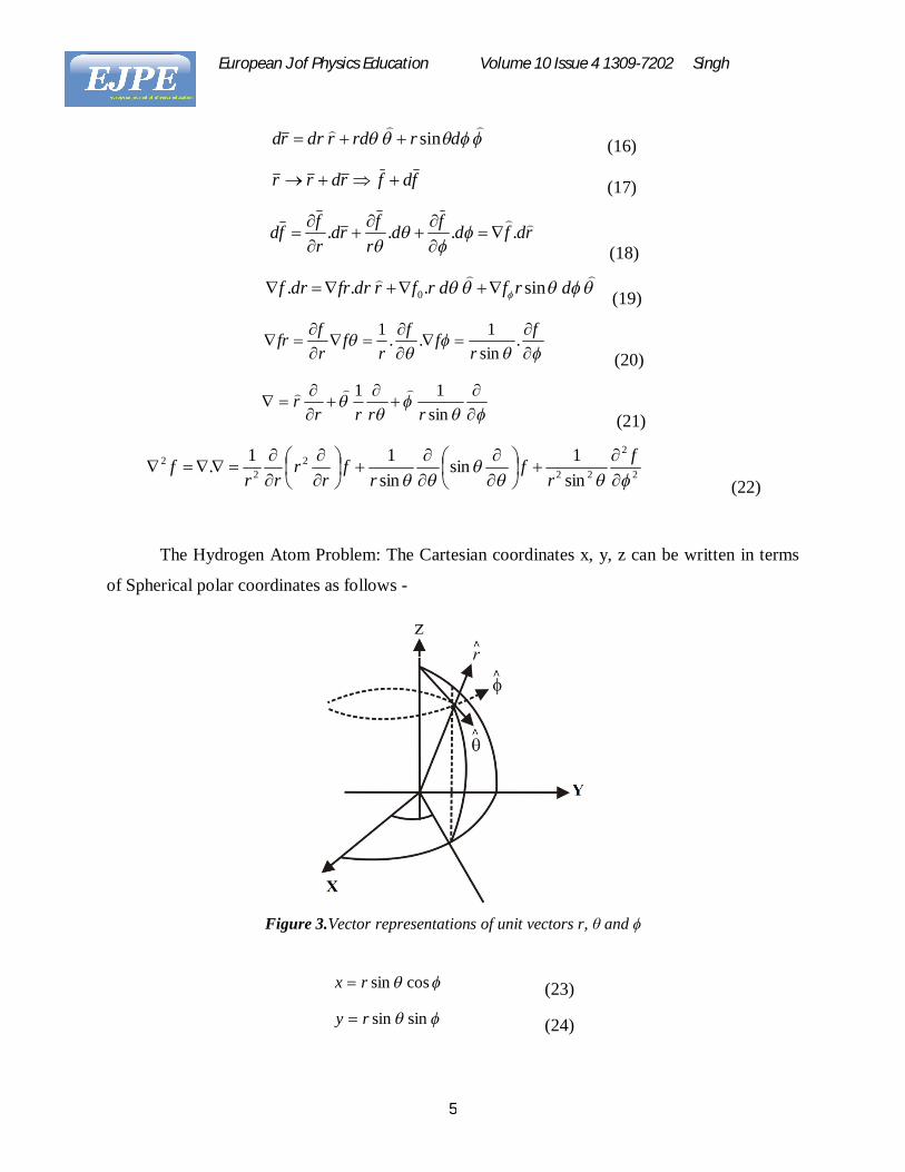
The Hydrogen Atom Problem: The Cartesian coordinates x, y, z can be written in terms
of Spherical polar coordinates as follows -
Figure 3.Vector representations of unit vectors r, θ and ϕ
cossinrx (23)
sinsinry (24)

European J of Physics Education Volume 10 Issue 4 1309-7202 Singh
6
cosrz (25)
Here, and are the angles made by the radial vector r, joining point P to the origin
and its components along X, Y and Z axis respectively Figure (4).
Figure 4. Radial vector r joining point P to the origin and its components along X, Y and Z axis
respectively
The Schrodinger equation in Spherical coordinates is given by:
0222
2
2
2
2
VEm
zyx (26)
The above Schrodinger equation in spherical polar co-ordinate system can be written as:
VEmrrr
rrr
22
2
222
2
2sin1sin
sin11
=0 (27)
We have,
reV
0
2
4
(28)
Multiply both sides of the above equation by 22 sinr , we get
04
sin2sinsinsin0
2
2
22
2
222
reEmr
rr
r
(29)
Using separation of variable, we can write the wave function as follow:

European J of Physics Education Volume 10 Issue 4 1309-7202 Singh
7
rr ,, (30)
Substituting as above and divide both sides of the equation by , we obtain -
0
4sin21sinsinsin
0
2
2
22
2
22
2
remr
rrr
rr
(31)
We can rearrange the terms as follows–
remr
rrr
rr 0
2
2
222
2
4sin2sinsinsin
(32)
2
21
The right hand side of the above equation is compared with the square of a quantum
number me -
22
21lm
(33)
022
2
lm (34)
This yields a solution -
mAe li (35)
Here, ml is called magnetic quantum number.
0lm , 1 , 2 , 3 , ………………
We can re-write the Schrodinger equation as –
remr
rrr
rr 0
2
2
22
2
42sin
rrml
sinsin 2
2
(36)
remr
rrr
rr 421 2
2
22
sin sin1
sin 2
2
rml
(37)
In above equation, we have obtained L.H.S. and R.H.S. as a function for r and co-
ordinates separately. Both sides give differential equations, which can be solved by comparing the equations with a constant. Here, in this case, it is 1ll . So, we have –
European J of Physics Education Volume 10 Issue 4 1309-7202 Singh
8
01
4211
20
2
22
2
rll
remr
rrr
(38)
0
sin1sin
sin1
2
2
lmllr (39)
The above equations can be re-written as follows -
014
212
0
2
22
2
r
rll
rem
rrr
rr (40)
0sin
1sin.sin
12
2
lmll
r (41)
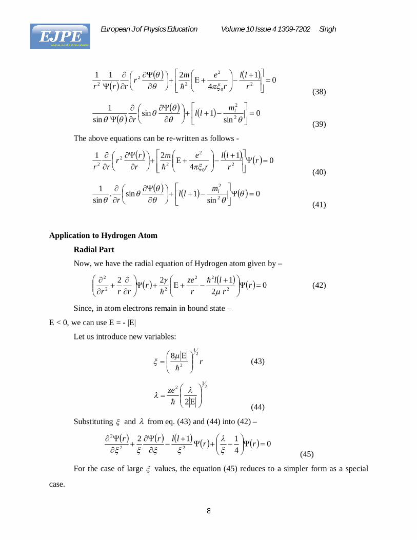
Application to Hydrogen Atom
Radial Part
Now, we have the radial equation of Hydrogen atom given by –
0 2
1222
22
22
2
r
rll
rzer
rrr
(42)
Since, in atom electrons remain in bound state –
E < 0, we can use E = - |E|
Let us introduce new variables:
r2
1
2
8
(43)
21
2
2
ze
(44)
Substituting and from eq. (43) and (44) into (42) –
04112
22
2
rrllrr
(45)
For the case of large values, the equation (45) reduces to a simpler form as a special
case.
European J of Physics Education Volume 10 Issue 4 1309-7202 Singh
9
041
2
2
rr (46)
The solution for eq. (46) is 2e , but the function must not diverge for , thus, the
acceptable general solution for bound state can be taken as –
ue .2 (47)
Substitution gives us –
011212 22
2
ulluu
(48)
Let us use a power series as a solution, such that –
n
rrnn Fau (49)
Substitution of eq. (49) into eq. (48) yields –
0111122
22
FlrrrFrF
(50)
As a trivial case, 0 , which yields
lr and 1 lr (51)
For finite solution at the origin, the acceptable solution is lr because r= (l-1) will make the series singular at 0
Now, eq. (50) becomes –
011222
2
FlFlF (52)
Substitution of F in form of a series gives –
011111
nnn allann
(53)
We obtain –
0
11 01221
n
nnn anlalnn
(54)
European J of Physics Education Volume 10 Issue 4 1309-7202 Singh
10
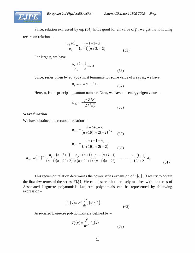
Since, relation expressed by eq. (54) holds good for all value of , we get the following
recursion relation –
22 111
lnnln
aa
n
n
(55)
For large n, we have
01~1
na
a
n
n
(56)
Since, series given by eq. (55) must terminate for some value of n say nr, we have.
1 lnn rp (57)
Here, np is the principal quantum number. Now, we have the energy eigen value –
22
42
2
pn n
eZEp
(58)
Wave function
We have obtained the recursion relation –
nn alnn
lna 22 1
11
(59)
22 11
1
lnl
nlna p
n (60)
lnn
lnnlnn
lnnlnn
lnna pppn
n 2 11
.12
.22 1
11 1
1
………. 0
22 .11 a
lln
(61)
This recursion relation determines the power series expansion of F . If we try to obtain the first few terms of the series F , We can observe that it closely matches with the terms of Associated Laguerre polynomials Laguerre polynomials can be represented by following expression –
xrr
rx
r exdxdexL
(62)
Associated Laguerre polynomials are defined by –
xLdxdxL q
qr 2
2
(63)

European J of Physics Education Volume 10 Issue 4 1309-7202 Singh
11
First few of the Laguerre polynomials are given as follows:
10 xL
xxL 11
22 42 xxxL
323 9186 xxxxL
Remember we have –
222
221
2221
2 cZec
ZeE
Z l
(64)
2
222
2ncxZ
ranZr
ncZr
neZcr
eEb
pp 222
222221
2
2248
(65)
The solution F is given by –
12 l
lnLF (66)
122,
l
lnl
ln Le (67)
The normalization of the wave function gives –
10
1222
lln
l LeA (68)
11
2 32
ln
lnnA
2
1
321
lnn
lnA (69)
So, the normalized radial wave function can be written as –
0
12
0
21
3
0,
22 2
120
naZrLe
naZr
lnnln
naZr l
lnna
zrl
ln
(70)
European J of Physics Education Volume 10 Issue 4 1309-7202 Singh
12
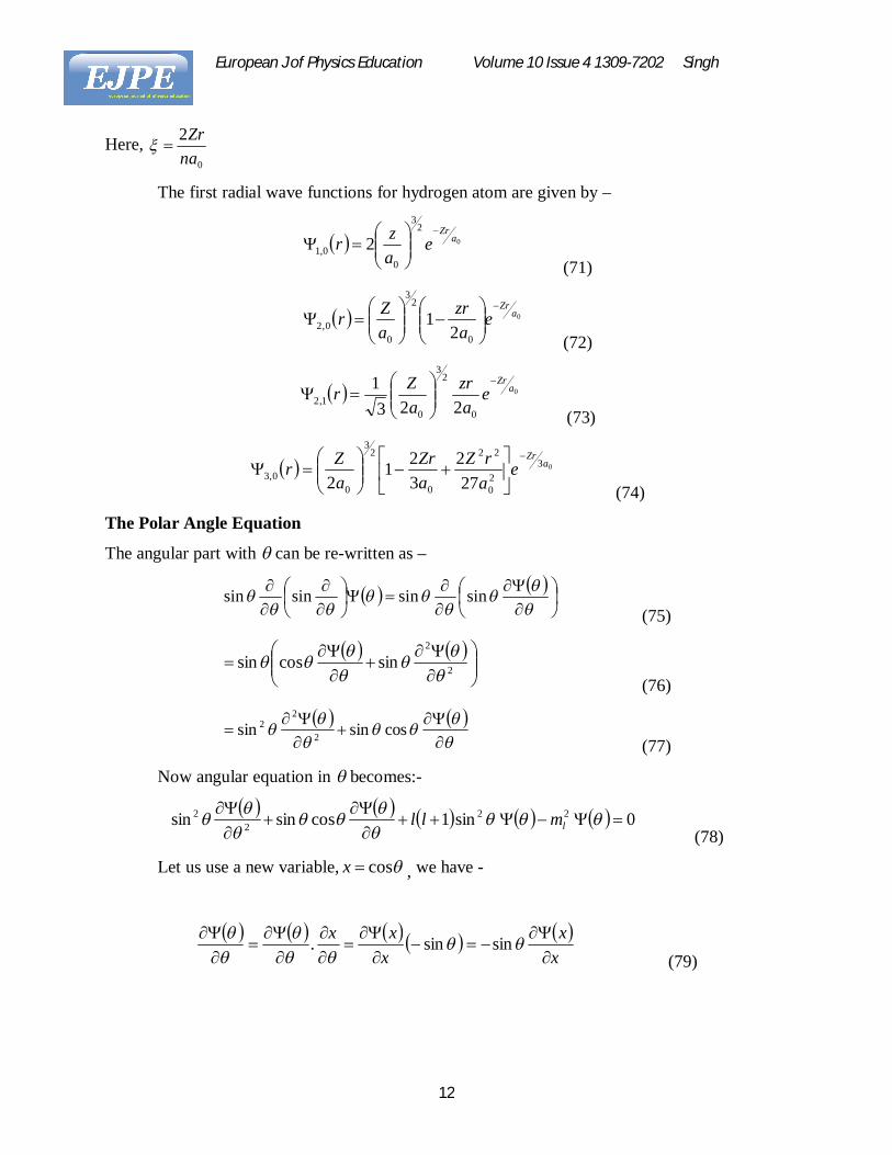
Here, 0
2naZr
The first radial wave functions for hydrogen atom are given by –
0
23
00,1 2 a
Zre
azr
(71)
0
0
23
00,2 2
1 aZr
eazr
aZr
(72)
0
0
23
01,2 223
1 aZr
eazr
aZr
(73)
0320
22
0
23
00,3 27
2321
2a
Zre
arZ
aZr
aZr
(74)
The Polar Angle Equation
The angular part with can be re-written as –
sinsinsinsin
(75)
2
2
sincossin
(76)
cossinsin 2
22
(77)
Now angular equation in becomes:-
0 sin1cossinsin 222
2
lmll (78)
Let us use a new variable, cosx , we have -
xx
xxx
sinsin .
(79)
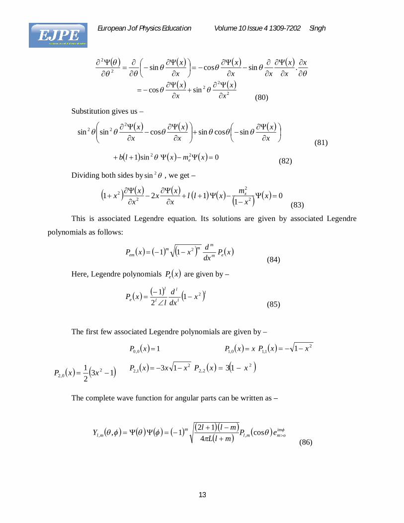
European J of Physics Education Volume 10 Issue 4 1309-7202 Singh
13
x
xx
xxx
xx .sincossin2
2
2
22sincos
xx
xx
(80)
Substitution gives us –
xx
xx
xx
sincossincossinsin2
22
(81)
0 sin1 22 xmxlb e (82)
Dividing both sides by 2sin , we get –
01
1 21 2
2
22
xx
mxllxxx
xxx x
(83)
This is associated Legendre equation. Its solutions are given by associated Legendre
polynomials as follows:
xPdxdxxP em
mmm
em211
(84)
Here, Legendre polynomials xPe are given by –
ll
l
l
l
e xdxd
lxP 21
21
(85)
The first few associated Legendre polynomials are given by –
10,0 xP xxP 0,1 21,1 1 xxP
21,2 13 xxxP 2
2,2 13 xxP
The complete wave function for angular parts can be written as –
im
ommlm
ml ePmlL
mllY
cos4
121 , ,,
(86)
1321 2
0,2 xxP
European J of Physics Education Volume 10 Issue 4 1309-7202 Singh
14
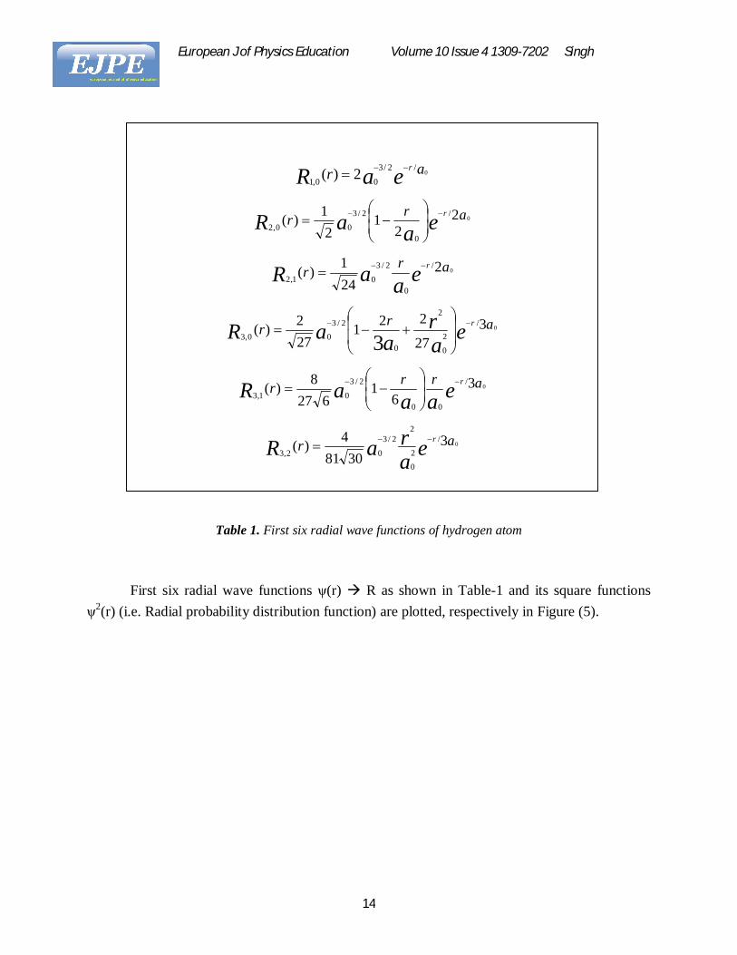
Table 1. First six radial wave functions of hydrogen atom
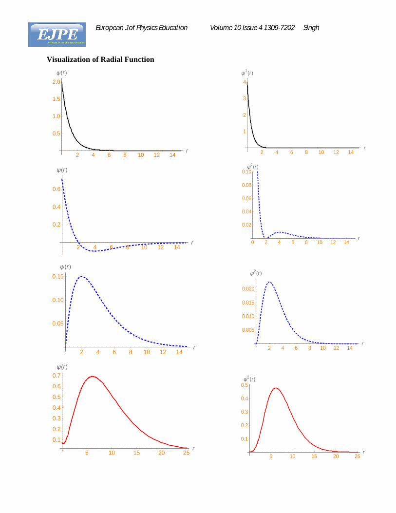
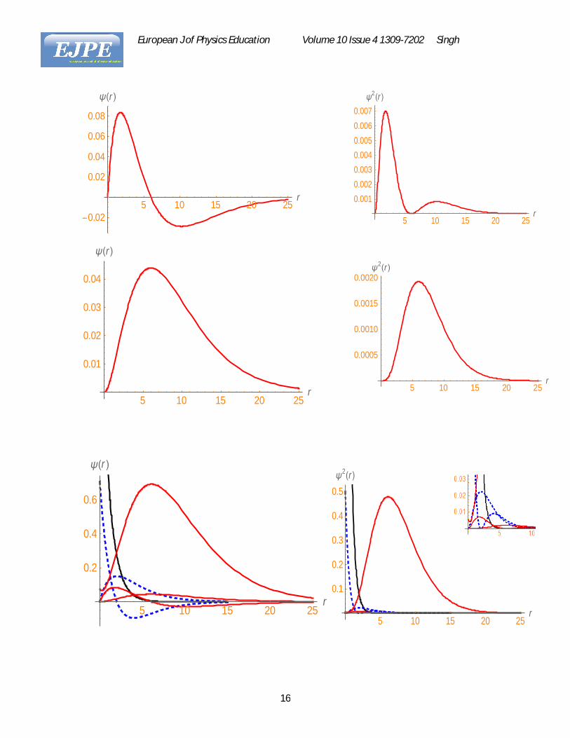
First six radial wave functions ψ(r) R as shown in Table-1 and its square functions ψ2(r) (i.e. Radial probability distribution function) are plotted, respectively in Figure (5).
eaR ar r0
/2/3
00,12)(
eaaR arr r 22
12
1)( 0/
0
2/3
00,2
eaaR arr r 2241)( 0
/
0
2/3
01,2
ear
aaR arr r 327
221272)( 0
/2
0
2
0
2/3
00,3 3
eaaaR arrr r 36
1627
8)( 0/
00
2/3
01,3
earaR ar r 3
30814)( 0
/
2
0
22/3
02,3
European J of Physics Education Volume 10 Issue 4 1309-7202 Singh
15
Visualization of Radial Function
2 4 6 8 10 12 14r
0.5
1.0
1.5
2.0r
2 4 6 8 10 12 14r
0.2
0.4
0.6
r
2 4 6 8 10 12 14r
0.05
0.10
0.15r
5 10 15 20 25r
0.1
0.2
0.3
0.4
0.5
0.6
0.7r
2 4 6 8 10 12 14r
1
2
3
4
2 r
0 2 4 6 8 10 12 14r
0.02
0.04
0.06
0.08
0.102 r
2 4 6 8 10 12 14r
0.005
0.010
0.015
0.020
2 r
5 10 15 20 25r
0.1
0.2
0.3
0.4
0.52 r
European J of Physics Education Volume 10 Issue 4 1309-7202 Singh
16
n=1, l=0, m=0
5 10 15 20 25r
0.02
0.02
0.04
0.06
0.08
r
5 10 15 20 25r
0.01
0.02
0.03
0.04
r
5 10 15 20 25r
0.0010.0020.0030.0040.0050.0060.007
2 r
5 10 15 20 25r
0.0005
0.0010
0.0015
0.00202 r
5 10 15 20 25
r
0.2
0.4
0.6
r
5 10 15 20 25r
0.1
0.2
0.3
0.4
0.5
2 r
European J of Physics Education Volume 10 Issue 4 1309-7202 Singh
17
Figure 5.First six radial wave functions ψ(r) R as shown in Table-1 and it’s square functions;ψ2(r) (i.e. Radial probability distribution function), respectively. These curves are plotted using Mathematica
Software.
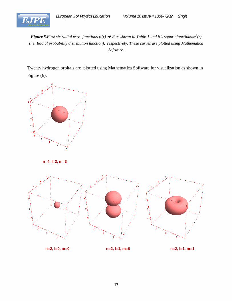
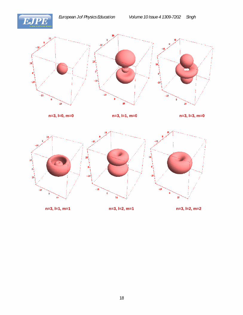
Twenty hydrogen orbitals are plotted using Mathematica Software for visualization as shown in Figure (6).
n=2, l=0, m=0 n=2, l=1, m=0 n=2, l=1, m=1
n=4, l=3, m=3
European J of Physics Education Volume 10 Issue 4 1309-7202 Singh
18
n=3, l=0, m=0 n=3, l=1, m=0 n=3, l=3, m=0
n=3, l=1, m=1 n=3, l=2, m=1 n=3, l=2, m=2

European J of Physics Education Volume 10 Issue 4 1309-7202 Singh
19
n=4, l=0, m=0 n=4, l=1, m=0 n=4, l=2, m=0
n=4, l=3, m=0 n=4, l=1, m=1 n=4, l=2, m=1
n=4, l=3, m=1 n=4, l=2, m=2 n=4, l=3, m=2

European J of Physics Education Volume 10 Issue 4 1309-7202 Singh
20
Figure 6. Twenty hydrogen orbitals are plotted using Mathematica Software for visualization. Their respective quantum numbers n, l and m are below the figures.
Readers may develop their own computer programs for Figure (5) and Figure (6) using available books (Wolfram 1996) on Mathematica Software .
CONCLUSION
The author hopes that the hierarchy of ideas systematically presented, will result into easy understanding of the problem,at under graduate level. The graphical presentations may encourage young students and their tutors to visualize the rigorous and comprehensive solutions, thus obtained, using Mathematica Software, and help them to grasp this important concept in order to apply quantum mechanics to more complicated physical problems.
Acknowledgements: Author is thankful to Abel Nazareth, Wolfram Research Inc., USA for providing trial license of Mathematica v.12.
n=4, l=3, m=3

European J of Physics Education Volume 10 Issue 4 1309-7202 Singh
21
REFERENCES
Alain, A. and Villain, J. (2017), The birth of wave mechanics (1923-1926), Comptes Rendus Physique, 18, 583-585.
Heisenberg, W. (1925), Über quantentheoretische Umdeutungkinematischer und mechanischer Beziehungen, Z. Phys. 33, 879.
Born, M. & Jordan, P. (1925), Zur Quantenmechanik, Z. Phys. 34, 858.
Aschman, D. &Keaney, B. (1989), The Legacy of Erwin Schrodinegr: Quantum Mechanics,Trans Roy. Soc. S. Africa, Part-I, 47, 81-101.
Reiter, W. L. &Yngvason, J. (2013), Erwin Schrodinger- 50 Years After, ESI Lectures in Mathematics and Physics, EuroepanMathemtical Society Publishing House.
Fedak, W. A. & Jeffrey, J. P. (2009), The 1925 Born and Jordan Paper “On Quantum Mechanics”, American Journal of Physics,77, 128.
Ghatak, A. & Loknathan, S. (2014), Qunatum Mechanics: Theory and Application (5th Ed.), Macmillan India.
Schiff, L. I. & Bandhyopadhyay, J. (2017), Quantum Mechanics (4th Ed.), McGraw Hill Education, India.
Fenyman, R., The Feynman Lectures on Physics, Volume III (1st Ed.), Pearson Education.
Retrieved from -http://www.astro.caltech.edu/~srk/Ay126/Lectures/Lecture3/SchrodingerModel.pdf,(Chapter-10 The Hydrogen Atom).
Wolfram, S. (1996), The Mathematica Book (3r. Ed.), Cambridge University Press, USA.