Solving Optimization Problems using the Matlab Optimization

Toolbox - a Tutorial

TU-Ilmenau, Fakultät für Mathematik und NaturwissenschaftenDr. Abebe Geletu

December 13, 2007

Contents

1 Introduction to Mathematical Programming 2

1.1 A general Mathematical Programming Problem . . . . . . . . . . . . . . . . . . . . . . 2

1.1.1 Some Classes of Optimization Problems . . . . . . . . . . . . . . . . . . . . . . 2

1.1.2 Functions of the Matlab Optimization Toolbox . . . . . . . . . . . . . . . . . . . 5

2 Linear Programming Problems 6

2.1 Linear programming with MATLAB . . . . . . . . . . . . . . . . . . . . . . . . . . . . . 6

2.2 The Interior Point Method for LP . . . . . . . . . . . . . . . . . . . . . . . . . . . . . . 8

2.3 Using linprog to solve LP’s . . . . . . . . . . . . . . . . . . . . . . . . . . . . . . . . . . 11

2.3.1 Formal problems . . . . . . . . . . . . . . . . . . . . . . . . . . . . . . . . . . . 11

2.3.2 Approximation of discrete Data by a Curve . . . . . . . . . . . . . . . . . . . . . 13

3 Quadratic programming Problems 15

3.1 Algorithms Implemented under quadprog.m . . . . . . . . . . . . . . . . . . . . . . . . 16

3.1.1 Active Set-Method . . . . . . . . . . . . . . . . . . . . . . . . . . . . . . . . . . 17

3.1.2 The Interior Reflective Method . . . . . . . . . . . . . . . . . . . . . . . . . . . 19

3.2 Using quadprog to Solve QP Problems . . . . . . . . . . . . . . . . . . . . . . . . . . . 24

3.2.1 Theoretical Problems . . . . . . . . . . . . . . . . . . . . . . . . . . . . . . . . . 24

3.2.2 Production model - profit maximization . . . . . . . . . . . . . . . . . . . . . . 26

4 Unconstrained nonlinear programming 30

4.1 Theory, optimality conditions . . . . . . . . . . . . . . . . . . . . . . . . . . . . . . . . 30

4.1.1 Problems, assumptions, definitions . . . . . . . . . . . . . . . . . . . . . . . . . 30

4.2 Optimality conditions for smooth unconstrained problems . . . . . . . . . . . . . . . . 31

4.3 Matlab Function for Unconstrained Optimization . . . . . . . . . . . . . . . . . . . . . 32

4.4 General descent methods - for differentiable Optimization Problems . . . . . . . . . . . 32

4.5 The Quasi-Newton Algorithm -idea . . . . . . . . . . . . . . . . . . . . . . . . . . . . . 33

4.5.1 Determination of Search Directions . . . . . . . . . . . . . . . . . . . . . . . . . 33

4.5.2 Line Search Strategies- determination of the step-length αk . . . . . . . . . . . 34

4.6 Trust Region Methods - idea . . . . . . . . . . . . . . . . . . . . . . . . . . . . . . . . . 35

4.6.1 Solution of the Trust-Region Sub-problem . . . . . . . . . . . . . . . . . . . . . 36

4.6.2 The Trust Sub-Problem under Considered in the Matlab Optimization toolbox . 38

4.6.3 Calling and Using fminunc.m to Solve Unconstrained Problems . . . . . . . . . 39

4.7 Derivative free Optimization - direct (simplex) search methods . . . . . . . . . . . . . . 45

1

Chapter 1

Introduction to Mathematical

Programming

1.1 A general Mathematical Programming Problem

f(x) −→ min (max)subject to

x ∈ M.(O)

The function f : Rn → R is called the objective function and the set M ⊂ R

n is the feasible set of (O).

Based on the description of the function f and the feasible set M , the problem (O) can be classified

as linear, quadratic, non-linear, semi-infinite, semi-definite, multiple-objective, discrete optimization

problem etc1.

1.1.1 Some Classes of Optimization Problems

Linear Programming

If the objective function f and the defining functions of M are linear, then (O) will be a linear

optimization problem.

General form of a linear programming problem:

c⊤x −→ min (max)s.t.Ax = aBx ≤ blb ≤ x ≤ ub;

(LO)

i.e. f(x) = c⊤x and M = x ∈ Rn | Ax = a,Bx ≤ b, lb ≤ x ≤ ub.

Under linear programming problems are such practical problems like: linear discrete Chebychev ap-

proximation problems, transportation problems, network flow problems,etc.

1The terminology mathematical programming is being currently contested and many demand that problems of the form

(O) be always called mathematical optimization problems. Here, we use both terms alternatively.

2

3

Quadratic Programming

12x

TQx+ q⊤x → mins.t.

Ax = aBx ≤ bx ≥ ux ≤ v

(QP)

Here the objective function f(x) = 12x⊤Qx + q⊤x is a quadratic function, while the feasible set

M = x ∈ Rn | Ax = a,Bx ≤ b, u ≤ x ≤ v is defined using linear functions.

One of the well known practical models of quadratic optimization problems is the least squares ap-

proximation problem; which has applications in almost all fields of science.

Non-linear Programming Problem

The general form of a non-linear optimization problem is

f (x) −→ min (max)subject to

equality constraints: gi (x) = 0, i ∈ 1, 2, . . . ,minequality constraints: gj (x) ≤ 0, j ∈ m+ 1,m+ 2, . . . ,m+ pbox constraints: uk ≤ xk ≤ vk, k = 1, 2, . . . , n;

(NLP)

where, we assume that all the function are smooth, i.e. the functions

f, gl : U −→ R l = 1, 2, . . . ,m+ p

are sufficiently many times differentiable on the open subset U of Rn. The feasible set of (NLP) is

given by

M = x ∈ Rn | gi(x) = 0, i = 1, 2, . . . ,m; gj(x) ≤ 0, j = m+ 1,m+ 2, . . . ,m+ p .

We also write the (NLP) in vectorial notation as

f (x) → min (max)

h (x) = 0

g (x) ≤ 0

u ≤ x ≤ v.

Problems of the form (NLP) arise frequently in the numerical solution of control problems, non-linear

approximation, engineering design, finance and economics, signal processing, etc.

4

Semi-infinite Programming

f(x) → mins.t.

G(x, y) ≤ 0,∀y ∈ Y ;hi(x) = 0, i = 1, . . . , p;gj(x) ≤ 0, j = 1, . . . , q;

x ∈ Rn;

Y ⊂ Rm.

(SIP)

Here, f, hi, gj : Rn → R, i ∈ 1, . . . , p, j ∈ 1, . . . , q are smooth functions; G : R

n × Rm → R is such

that, for each fixed y ∈ Y , G(·, y) : Rn → R is smooth and, for each fixed x ∈ R

n, G(x, ·) : Rm → R is

smooth; furthermore, Y is a compact subset of Rm. Sometimes, the set Y can also be given as

Y = y ∈ Rm | uk(y) = 0, k = 1, . . . , s1; vl(y) ≤ 0, l = 1, . . . , s2

with smooth functions uk, vl : Rm → R, k ∈ 1, . . . , s1, l ∈ 1, . . . , s2.

The problem (SIP) is called semi-infinite, since its an optimization problem with finite number of vari-

ables (i.e. x ∈ Rn) and infinite number of constraints (i.e. G(x, y) ≤ 0,∀y ∈ Y ).

One of the well known practical models of (SIP) is the continuous Chebychev approximation problem.

This approximation problem can be used for the approximation of functions by polynomials, in filter

design for digital signal processing, spline approximation of robot trajectory

Multiple-Objective Optimization

A multiple objective Optimization problem has a general form

min(f1(x), f1(x), . . . , fm(x))s.t.

x ∈M ;(MO)

where the functions fk : Rn → R, k = 1, . . . ,m are smooth and the feasible setM is defined in terms of

linear or non-linear functions. Sometimes, this problem is also alternatively called multiple-criteria,

vector optimization, goal attainment or multi-decision analysis problem. It is an optimization

problem with more than one objective function (each such objective is a criteria). In this sense,

(LO),(QP)(NLO) and (SIP) are single objective (criteria) optimization problems. If there are only two

objective functions in (MO), then (MO) is commonly called to be a bi-criteria optimization problem.

Furthermore, if each of the functions f1, . . . , fm are linear and M is defined using linear functions,

then (MO) will be a linear multiple-criteria optimization problem; otherwise, it is non-linear.

For instance, in a financial application we may need, to maximize revenue and minimize risk at the

same time, constrained upon the amount of our investment. Several engineering design problems can

also be modeled into (MO). Practical problems like autonomous vehicle control, optimal truss design,

antenna array design, etc are very few examples of (MO).

In real life we may have several objectives to arrive at. But, unfortunately, we cannot satisfy all

our objectives optimally at the same time. So we have to find a compromising solution among all

our objectives. Such is the nature of multiple objective optimization. Thus, the minimization (or

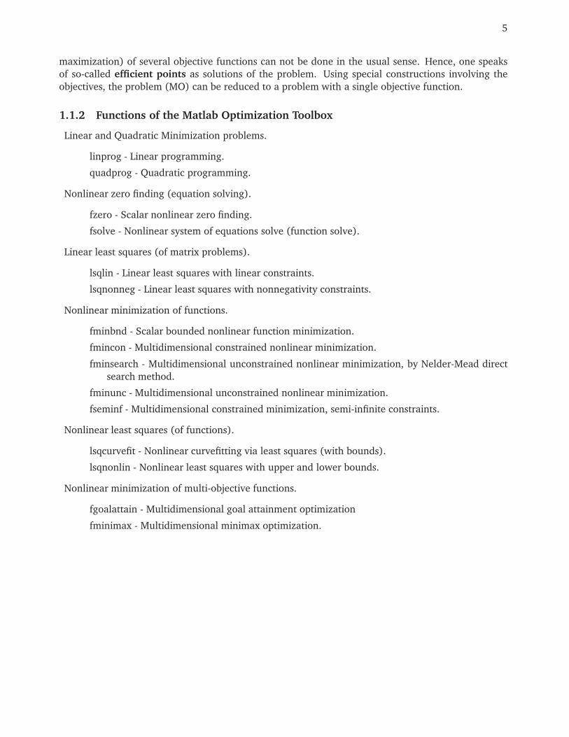
5

maximization) of several objective functions can not be done in the usual sense. Hence, one speaks

of so-called efficient points as solutions of the problem. Using special constructions involving the

objectives, the problem (MO) can be reduced to a problem with a single objective function.

1.1.2 Functions of the Matlab Optimization Toolbox

Linear and Quadratic Minimization problems.

linprog - Linear programming.

quadprog - Quadratic programming.

Nonlinear zero finding (equation solving).

fzero - Scalar nonlinear zero finding.

fsolve - Nonlinear system of equations solve (function solve).

Linear least squares (of matrix problems).

lsqlin - Linear least squares with linear constraints.

lsqnonneg - Linear least squares with nonnegativity constraints.

Nonlinear minimization of functions.

fminbnd - Scalar bounded nonlinear function minimization.

fmincon - Multidimensional constrained nonlinear minimization.

fminsearch - Multidimensional unconstrained nonlinear minimization, by Nelder-Mead direct

search method.

fminunc - Multidimensional unconstrained nonlinear minimization.

fseminf - Multidimensional constrained minimization, semi-infinite constraints.

Nonlinear least squares (of functions).

lsqcurvefit - Nonlinear curvefitting via least squares (with bounds).

lsqnonlin - Nonlinear least squares with upper and lower bounds.

Nonlinear minimization of multi-objective functions.

fgoalattain - Multidimensional goal attainment optimization

fminimax - Multidimensional minimax optimization.

Chapter 2

Linear Programming Problems

2.1 Linear programming with MATLAB

For the linear programming problem

c⊤x −→ mins.t.Ax ≤ aBx = blb ≤ x ≤ ub;

(LP)

MATLAB: The program linprog.m is used for the minimization of problems of the form (LP).

Once you have defined the matrices A, B, and the vectors c,a,b,lb and ub, then you can call linprog.m

to solve the problem. The general form of calling linprog.m is:

[x,fval,exitflag,output,lambda]=linprog(f,A,a,B,b,lb,ub,x0,options)

Input arguments:

c coefficient vector of the objective

A Matrix of inequality constraints

a right hand side of the inequality constraints

B Matrix of equality constraints

b right hand side of the equality constraints

lb,[ ] lb ≤ x : lower bounds for x, no lower bounds

ub,[ ] x ≤ ub : upper bounds for x, no upper bounds

x0 Startvector for the algorithm, if known, else [ ]

options options are set using the optimset funciton, they determine what algorism to use,etc.

Output arguments:

x optimal solution

fval optimal value of the objective function

exitflag tells whether the algorithm converged or not, exitflag > 0 means convergence

output a struct for number of iterations, algorithm used and PCG iterations(when LargeScale=on)

lambda a struct containing lagrange multipliers corresponding to the constraints.

6

7

Setting Options

The input argument options is a structure, which contains several parameters that you can use with

a given Matlab optimization routine.

For instance, to see the type of parameters you can use with the linprog.m routine use

>>optimset(’linprog’)

Then Matlab displays the fileds of the structure options. Accordingly, before calling linprog.m you

can set your preferred parameters in the options for linprog.m using the optimset command as:

>>options=optimset(’ParameterName1’,value1,’ParameterName2’,value2,...)

where ’ParameterName1’,’ParameterName2’,... are those you get displayed when you use

optimset(’linprog’). And value1, value2,... are their corresponding values.

The following are parameters and their corresponding values which are frequently used with linprog.m:

Parameter Possible Values

’LargeScale’ ’on’,’off’

’Simplex’ ’on’,’off’

’Display’ ’iter’,’final’,’off’

’Maxiter’ Maximum number of iteration

’TolFun’ Termination tolerance for the objective function

’TolX’ Termination tolerance for the iterates

’Diagnostics’ ’on’ or ’off’ (when ’on’ prints diagnostic information about the objective function)

Algorithms under linprog

There are three type of algorithms that are being implemented in the linprog.m:

• a simplex algorithm;

• an active-set algorithm;

• a primal-dual interior point method.

The simplex and active-set algorithms are usually used to solve medium-scale linear programming

problems. If any one of these algorithms fail to solve a linear programming problem, then the problem

at hand is a large scale problem. Moreover, a linear programming problem with several thousands of

variables along with sparse matrices is considered to be a large-scale problem. However, if coefficient

matrices of your problem have a dense matrix structure, then linprog.m assumes that your problem

is of medium-scale.

By default, the parameter ’LargeScale’ is always ’on’. When ’LargeScale’ is ’on’, then linprog.m

uses the primal-dual interior point algorithm. However, if you want to set if off so that you can solve

a medium scale problem , then use

>>options=optimset(’LargeScale’,’off’)

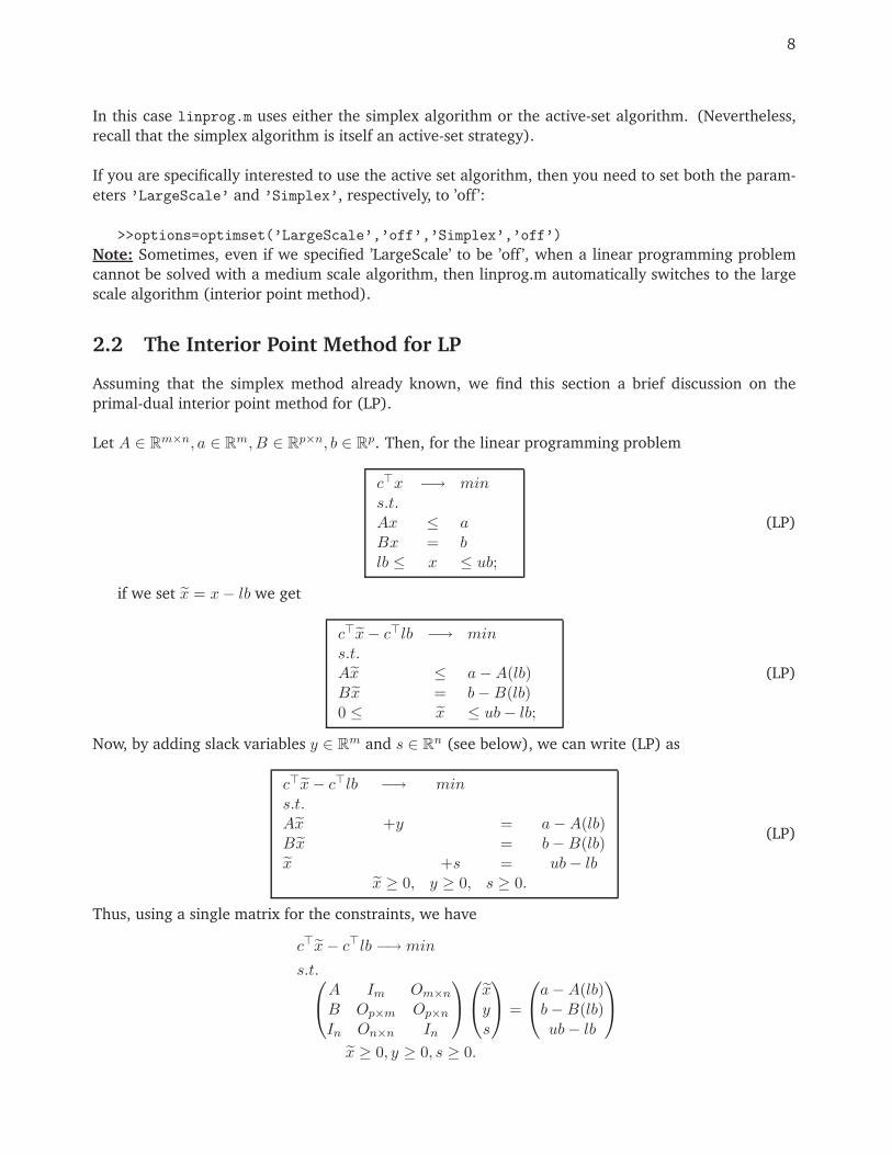
8

In this case linprog.m uses either the simplex algorithm or the active-set algorithm. (Nevertheless,

recall that the simplex algorithm is itself an active-set strategy).

If you are specifically interested to use the active set algorithm, then you need to set both the param-

eters ’LargeScale’ and ’Simplex’, respectively, to ’off’:

>>options=optimset(’LargeScale’,’off’,’Simplex’,’off’)

Note: Sometimes, even if we specified ’LargeScale’ to be ’off’, when a linear programming problem

cannot be solved with a medium scale algorithm, then linprog.m automatically switches to the large

scale algorithm (interior point method).

2.2 The Interior Point Method for LP

Assuming that the simplex method already known, we find this section a brief discussion on the

primal-dual interior point method for (LP).

Let A ∈ Rm×n, a ∈ R

m, B ∈ Rp×n, b ∈ R

p. Then, for the linear programming problem

c⊤x −→ mins.t.Ax ≤ aBx = blb ≤ x ≤ ub;

(LP)

if we set x = x− lb we get

c⊤x− c⊤lb −→ mins.t.Ax ≤ a−A(lb)Bx = b−B(lb)0 ≤ x ≤ ub− lb;

(LP)

Now, by adding slack variables y ∈ Rm and s ∈ R

n (see below), we can write (LP) as

c⊤x− c⊤lb −→ mins.t.Ax +y = a−A(lb)Bx = b−B(lb)x +s = ub− lb

x ≥ 0, y ≥ 0, s ≥ 0.

(LP)

Thus, using a single matrix for the constraints, we have

c⊤x− c⊤lb −→ min

s.t.A Im Om×n

B Op×m Op×n

In On×n In

xys

=

a−A(lb)b−B(lb)ub− lb

x ≥ 0, y ≥ 0, s ≥ 0.

9

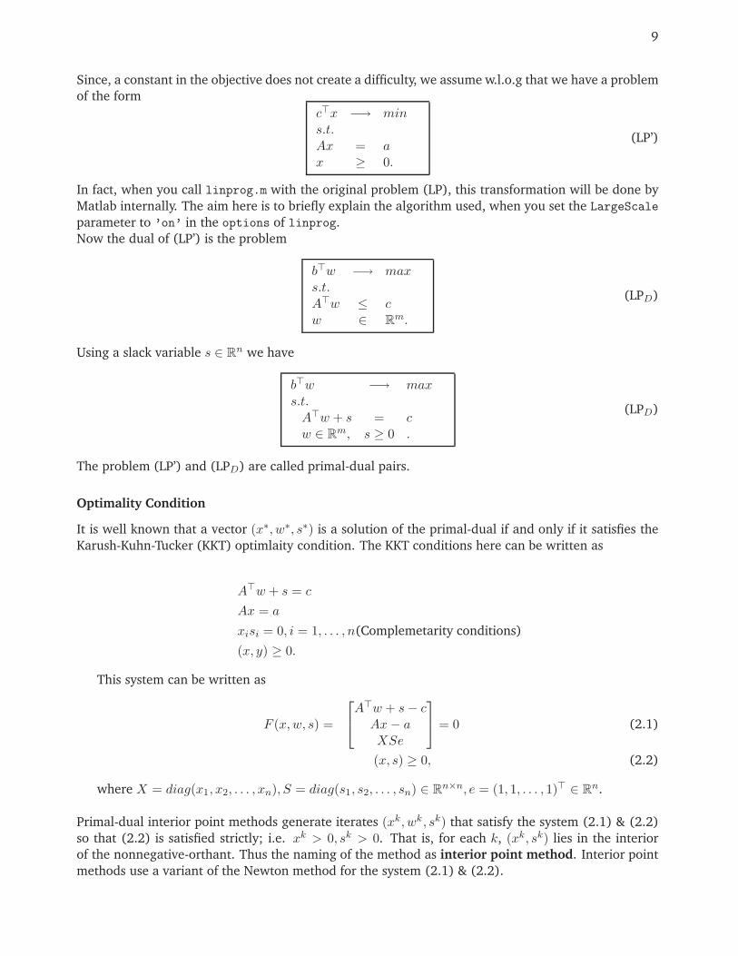
Since, a constant in the objective does not create a difficulty, we assume w.l.o.g that we have a problem

of the form

c⊤x −→ mins.t.Ax = ax ≥ 0.

(LP’)

In fact, when you call linprog.m with the original problem (LP), this transformation will be done by

Matlab internally. The aim here is to briefly explain the algorithm used, when you set the LargeScale

parameter to ’on’ in the options of linprog.

Now the dual of (LP’) is the problem

b⊤w −→ maxs.t.A⊤w ≤ cw ∈ R

m.

(LPD)

Using a slack variable s ∈ Rn we have

b⊤w −→ maxs.t.A⊤w + s = cw ∈ R

m, s ≥ 0 .

(LPD)

The problem (LP’) and (LPD) are called primal-dual pairs.

Optimality Condition

It is well known that a vector (x∗, w∗, s∗) is a solution of the primal-dual if and only if it satisfies the

Karush-Kuhn-Tucker (KKT) optimlaity condition. The KKT conditions here can be written as

A⊤w + s = c

Ax = a

xisi = 0, i = 1, . . . , n(Complemetarity conditions)

(x, y) ≥ 0.

This system can be written as

F (x,w, s) =

A⊤w + s− cAx− aXSe

= 0 (2.1)

(x, s) ≥ 0, (2.2)

where X = diag(x1, x2, . . . , xn), S = diag(s1, s2, . . . , sn) ∈ Rn×n, e = (1, 1, . . . , 1)⊤ ∈ R

n.

Primal-dual interior point methods generate iterates (xk, wk, sk) that satisfy the system (2.1) & (2.2)

so that (2.2) is satisfied strictly; i.e. xk > 0, sk > 0. That is, for each k, (xk, sk) lies in the interior

of the nonnegative-orthant. Thus the naming of the method as interior point method. Interior point

methods use a variant of the Newton method for the system (2.1) & (2.2).

10

Central Path

Let τ > 0 be a parameter. The central path is a curve C which is the set of all points (x(τ), w(τ), s(τ)) ∈C that satisfy the parametric system :

A⊤w + s = c,

Ax = b,

xsi = τ, i = 1, . . . , n

(x, s) > 0.

This implies C is the set of all points (x(τ), w(τ), s(τ)) that satisfy

F (x(τ), w(τ), s(τ)) =

00τe

, (x(τ), s(τ)) > 0. (2.3)

Obviously, if we let τ ↓ 0, the the system (2.3) goes close to the system (2.1) & (2.2).

Hence, theoretically, primal-dual algorithms solve the system

J(x(τ), w(τ), s(τ))

x(τ)w(τ)s(τ)

=

00

−XSe+ τe

to determine a search direction (x(τ),w(τ),s(τ)), where J(x(τ), w(τ), s(τ)) is the Jacobian of

F (x(τ), w(τ), s(τ)). And the new iterate will be

(x+(τ), w+(τ), s+(τ)) = (x(τ), w(τ), s(τ)) + α(x(τ),w(τ),s(τ)),

where α is a step length, usually α ∈ (0, 1], chosen in such a way that (x+(τ), w+(τ), s+(τ) ∈ C.

However, practical primal-dual interior point methods use τ = σµ, where σ ∈ [0, 1] is a constant and

µ =x⊤s

n

The term x⊤s is the duality gap between the primal and dual problems. Thus, µ is the measure of

the (average) duality gap. Note that, in general, µ ≥ 0 and µ = 0 when x and s are primal and dual

optimal, respectively.

Thus the Newton step (x(µ),w(µ),s(µ)) is determined by solving:

On A⊤ InA On×m Om×n

S On×m X

x(τ)w(τ)s(τ)

=

00

−XSe+ σµe

. (2.4)

The Newton step (x(µ),w(µ),s(µ)) is also called centering direction that pushes the iterates

(x+(µ), w+(µ), s+(µ) towards the central path C along which the algorithm converges more rapidly.

The parameter σ is called the centering parameter. If σ = 0, then the search direction is known to

be an affine scaling direction.

Primal-Dual Interior Point Algorithm

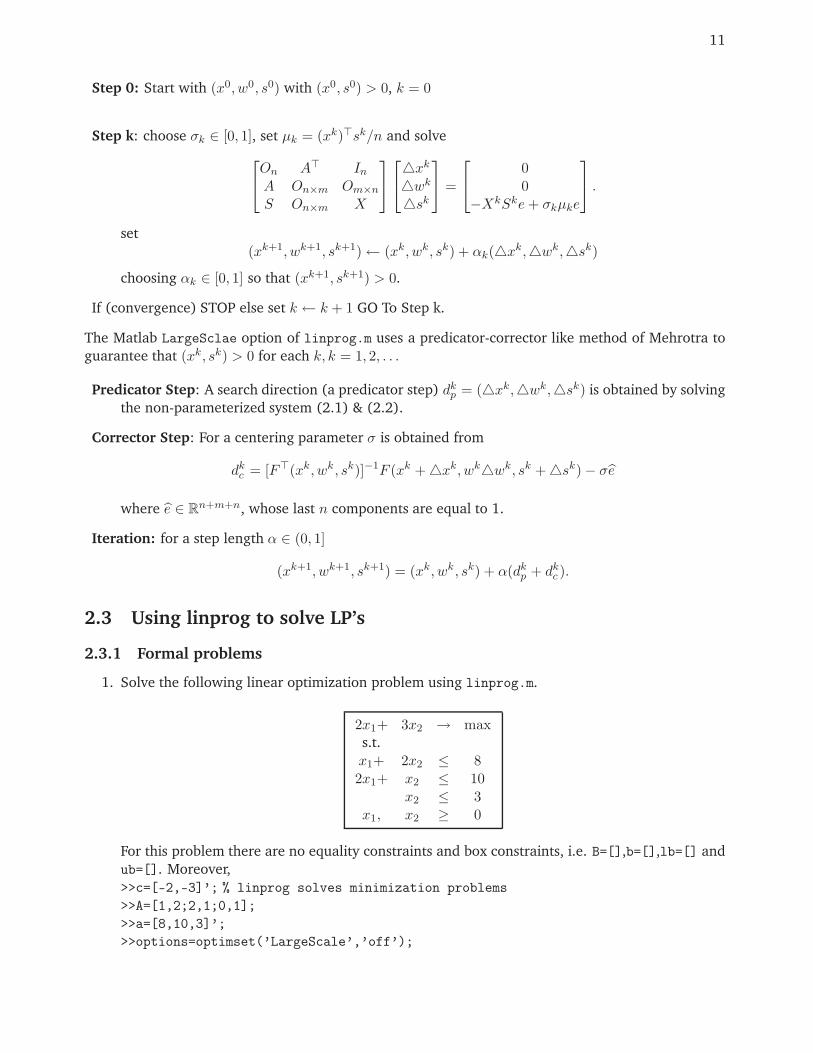
11

Step 0: Start with (x0, w0, s0) with (x0, s0) > 0, k = 0

Step k: choose σk ∈ [0, 1], set µk = (xk)⊤sk/n and solve

On A⊤ InA On×m Om×n

S On×m X

xk

wk

sk

=

00

−XkSke+ σkµke

.

set

(xk+1, wk+1, sk+1)← (xk, wk, sk) + αk(xk,wk,sk)

choosing αk ∈ [0, 1] so that (xk+1, sk+1) > 0.

If (convergence) STOP else set k ← k + 1 GO To Step k.

The Matlab LargeSclae option of linprog.m uses a predicator-corrector like method of Mehrotra to

guarantee that (xk, sk) > 0 for each k, k = 1, 2, . . .

Predicator Step: A search direction (a predicator step) dkp = (xk,wk,sk) is obtained by solving

the non-parameterized system (2.1) & (2.2).

Corrector Step: For a centering parameter σ is obtained from

dkc = [F⊤(xk, wk, sk)]−1F (xk +xk, wkwk, sk +sk)− σe

where e ∈ Rn+m+n, whose last n components are equal to 1.

Iteration: for a step length α ∈ (0, 1]

(xk+1, wk+1, sk+1) = (xk, wk, sk) + α(dkp + dk

c ).

2.3 Using linprog to solve LP’s

2.3.1 Formal problems

1. Solve the following linear optimization problem using linprog.m.

2x1+ 3x2 → maxs.t.

x1+ 2x2 ≤ 82x1+ x2 ≤ 10

x2 ≤ 3x1, x2 ≥ 0

For this problem there are no equality constraints and box constraints, i.e. B=[],b=[],lb=[] and

ub=[]. Moreover,

>>c=[-2,-3]’; % linprog solves minimization problems

>>A=[1,2;2,1;0,1];

>>a=[8,10,3]’;

>>options=optimset(’LargeScale’,’off’);

12

i) If you are interested only on the solution, then use

>>xsol=linprog(c,A,b,[],[],[],[],[],options)

ii) To see if the algorithm really converged or not you need to access the exit flag through:

>>[xsol,fval,exitflag]=linprog(c,A,a,[],[],[],[],[],options)

iii) If you need the Lagrange multipliers you can access them using:

>>[xsol,fval,flag,output,LagMult]=linprog(c,A,a,[],[],[],[],[],options)

iv) To display the iterates you can use:

>>xsol=linprog(c,A,a,[],[],[],[],[],optimset(’Display’,’iter’))

2. Solve the following LP using linprog.m

c⊤x −→ maxAx = aBx ≥ bDx ≤ d

lb ≤ x ≤ lu

where

(A| a) =

(1 1 1 1 1 15 0 −3 0 1 0

∣∣∣∣1015

), (B| b) =

1 2 3 0 0 00 1 2 3 0 00 0 1 2 3 00 0 0 1 2 3

∣∣∣∣∣∣∣∣

5788

,

(D| d) =

(3 0 0 0 −2 10 4 0 −2 0 3

∣∣∣∣57

), lb =

−20−1−1−5

1

, lu =

72234

10

, c =

1−2

3−4

5−6

.

When there are large matrices, it is convenient to write m files. Thus one possible solution will

be the following:

function LpExa2

A=[1,1,1,1,1,1;5,0,-3,0,1,0]; a=[10,15]’;

B1=[1,2,3,0,0,0; 0,1,2,3,0,0;... 0,0,1,2,3,0;0,0,0,1,2,3]; b1=[5,7,8,8];b1=b1(:);

D=[3,0,0,0,-2,1;0,4,0,-2,0,3]; d=[5,7]; d=d(:);

lb=[-2,0,-1,-1,-5,1]’; ub=[7,2,2,3,4,10]’;

c=[1,-2,3,-4,5,-6];c=c(:);

B=[-B1;D]; b=[-b1;d];

[xsol,fval,exitflag,output]=linprog(c,A,a,B,b,lb,ub)

fprintf(’%s %s \n’, ’Algorithm Used: ’,output.algorithm);

disp(’=================================’);

disp(’Press Enter to continue’); pause

options=optimset(’linprog’);

13

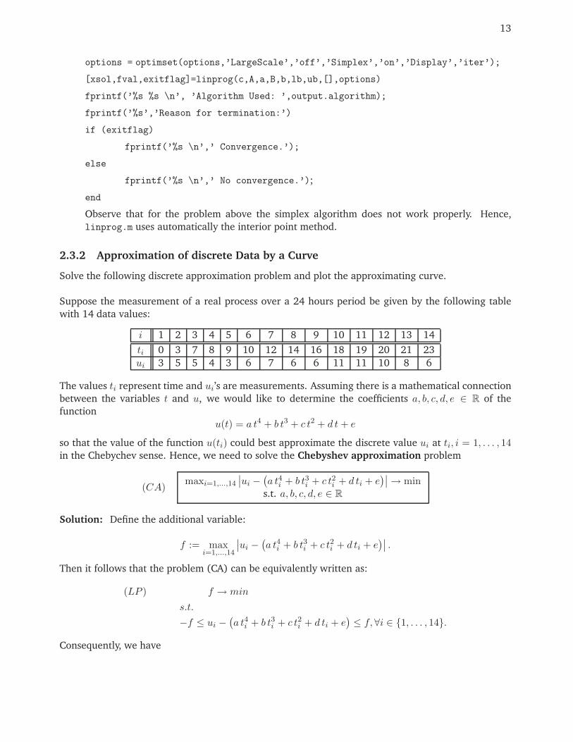
options = optimset(options,’LargeScale’,’off’,’Simplex’,’on’,’Display’,’iter’);

[xsol,fval,exitflag]=linprog(c,A,a,B,b,lb,ub,[],options)

fprintf(’%s %s \n’, ’Algorithm Used: ’,output.algorithm);

fprintf(’%s’,’Reason for termination:’)

if (exitflag)

fprintf(’%s \n’,’ Convergence.’);

else

fprintf(’%s \n’,’ No convergence.’);

end

Observe that for the problem above the simplex algorithm does not work properly. Hence,

linprog.m uses automatically the interior point method.

2.3.2 Approximation of discrete Data by a Curve

Solve the following discrete approximation problem and plot the approximating curve.

Suppose the measurement of a real process over a 24 hours period be given by the following table

with 14 data values:

i 1 2 3 4 5 6 7 8 9 10 11 12 13 14

ti 0 3 7 8 9 10 12 14 16 18 19 20 21 23

ui 3 5 5 4 3 6 7 6 6 11 11 10 8 6

The values ti represent time and ui’s are measurements. Assuming there is a mathematical connection

between the variables t and u, we would like to determine the coefficients a, b, c, d, e ∈ R of the

function

u(t) = a t4 + b t3 + c t2 + d t + e

so that the value of the function u(ti) could best approximate the discrete value ui at ti, i = 1, . . . , 14in the Chebychev sense. Hence, we need to solve the Chebyshev approximation problem

(CA)maxi=1,...,14

∣∣ui −(a t4i + b t3i + c t2i + d ti + e

)∣∣→ mins.t. a, b, c, d, e ∈ R

Solution: Define the additional variable:

f := maxi=1,...,14

∣∣ui −(a t4i + b t3i + c t2i + d ti + e

)∣∣ .

Then it follows that the problem (CA) can be equivalently written as:

(LP ) f → min

s.t.

−f ≤ ui −(a t4i + b t3i + c t2i + d ti + e

)≤ f,∀i ∈ 1, . . . , 14.

Consequently, we have

14

(LP ) f → min

s.t.

−(a t4i + b t3i + c t2i + d ti + e

)− f ≤ −ui,∀i ∈ 1, . . . , 14(

a t4i + b t3i + c t2i + d ti + e)− f ≤ ui,∀i ∈ 1, . . . , 14.

The solution is provide in the following m-file:

function ChebApprox1

%ChebApprox1:

% Solves a discrete Chebychev polynomial

% approximation Problem

t=[0,3,7,8,9,10,12,14,16,18,19,20,21,23]’;

u=[3,5,5,4,3,6,7,6,6,11,11,10,8,6]’;

A1=[-t.^4,-t.^3,-t.^2,-t,-ones(14,1),-ones(14,1)];

A2=[t.^4,t.^3,t.^2,t,ones(14,1),-ones(14,1)];

c=zeros(6,1); c(6)=1; %objective function coefficient

A=[A1;A2];%inequality constraint matrix

a=[-u;u];%right hand side vectro of ineq constraints

[xsol,fval,exitflag]=linprog(c,A,a);

%%%%next plot the Data points and the function %%%%%%%%%

plot(t,u,’r*’); hold on tt=[0:0.5:25];

ut=xsol(1)*(tt.^4)+xsol(2)*(tt.^3)+xsol(3)*(tt.^2)+xsol(4)*tt+...

xsol(5);

plot(tt,ut,’-k’,’LineWidth’,2)

Chapter 3

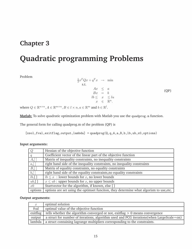
Quadratic programming Problems

Problem12x

TQx+ qTx → mins.t.

Ax ≤ aBx = blb ≤ x ≤ lux ∈ R

n.

(QP)

where Q ∈ Rn×n, A ∈ R

m×n, B ∈ l × n, a ∈ Rm and b ∈ R

l.

Matlab: To solve quadratic optimization problem with Matlab you use the quadprog.m function.

The general form for calling quadprog.m of the problem (QP) is

[xsol,fval,exitflag,output,lambda] = quadprog(Q,q,A,a,B,b,lb,ub,x0,options)

Input arguments:

Q Hessian of the objective function

q Coefficient vector of the linear part of the objective function

A,[ ] Matrix of inequality constraints, no inequality constraints

a,[ ] right hand side of the inequality constraints, no inequality constraints

B,[ ] Matrix of equality constraints, no equality constraints

b,[ ] right hand side of the equality constraints,no equality constraints

lb,[ ] lb ≤ x : lower bounds for x, no lower bounds

ub,[ ] x ≤ ub : upper bounds for x, no upper bounds

x0 Startvector for the algorithm, if known, else [ ]

options options are set using the optimset funciton, they determine what algorism to use,etc.

Output arguments:

x optimal solution

fval optimal value of the objective function

exitflag tells whether the algorithm converged or not, exitflag > 0 means convergence

output a struct for number of iterations, algorithm used and PCG iterations(when LargeScale=on)

lambda a struct containing lagrange multipliers corresponding to the constraints.

15

16

There are specific parameter settings that that you can use with the quadprog.m funciton. To see the

options parameter for quadprog.m along with their default values you can use

>>optimset(’quadprog’)

Then Matlab displays a structure containing the options related with quadprog.m function. Obsever

that, in contrast to linprog.m, the fields

options.MaxIter, options.TolFun options.TolX, options.TolPCG

posses default values in the quadprog.m.

With quadrprog.m you can solve large-scale and a medium-scale quadratic optimization problems. For

instance, to specify that you want to use the medium-scale algorithm:

>>oldOptions=optimset(’quadprog’);

>>options=optimset(oldOptions,’LargeScale’,’off’);

The problem (QP) is assumed to be large-scale:

• either if there are no equality and inequality constraints; i.e. if there are only lower and upper

bound constraints;12x

TQx+ qTx → mins.t.

lb ≤ x ≤ lu(QP)

• or if there are only linear equality constraints.

12x

TQx+ qTx → mins.t.

Ax ≤ ax ∈ R

n.

(QP)

In all other cases (QP) is assumed to be medium-scale.

For a detailed description of the quadprog.m use

>>doc quadprog

3.1 Algorithms Implemented under quadprog.m

(a) Medium-Scale algorithm: Active-set strategy.

(b) Large-Scale algorithm: an interior reflective Newton method coupled with a trust region method.

17

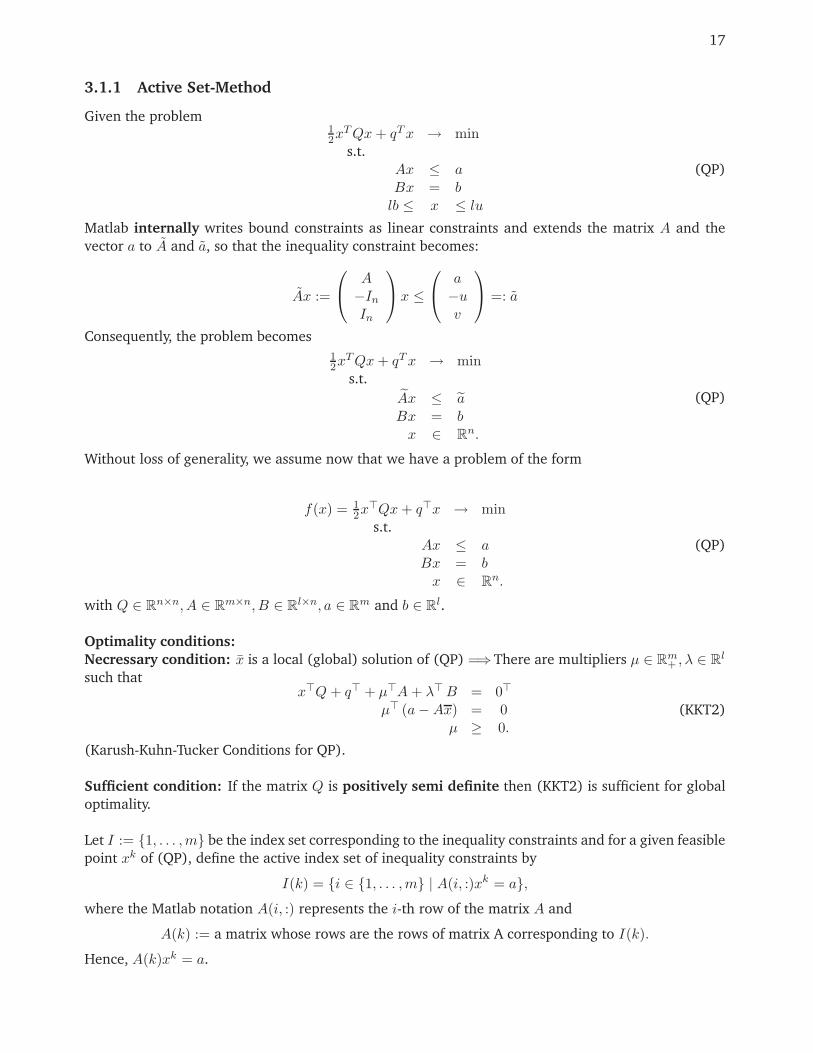
3.1.1 Active Set-Method

Given the problem12x

TQx+ qTx → mins.t.

Ax ≤ aBx = blb ≤ x ≤ lu

(QP)

Matlab internally writes bound constraints as linear constraints and extends the matrix A and the

vector a to A and a, so that the inequality constraint becomes:

Ax :=

A−InIn

x ≤

a−uv

=: a

Consequently, the problem becomes

12x

TQx+ qTx → mins.t.

Ax ≤ aBx = bx ∈ R

n.

(QP)

Without loss of generality, we assume now that we have a problem of the form

f(x) = 12x

⊤Qx+ q⊤x → mins.t.

Ax ≤ aBx = bx ∈ R

n.

(QP)

with Q ∈ Rn×n, A ∈ R

m×n, B ∈ Rl×n, a ∈ R

m and b ∈ Rl.

Optimality conditions:

Necressary condition: x is a local (global) solution of (QP) =⇒There are multipliers µ ∈ Rm+ , λ ∈ R

l

such thatx⊤Q+ q⊤ + µ⊤A+ λ⊤B = 0⊤

µ⊤ (a−Ax) = 0µ ≥ 0.

(KKT2)

(Karush-Kuhn-Tucker Conditions for QP).

Sufficient condition: If the matrix Q is positively semi definite then (KKT2) is sufficient for global

optimality.

Let I := 1, . . . ,m be the index set corresponding to the inequality constraints and for a given feasible

point xk of (QP), define the active index set of inequality constraints by

I(k) = i ∈ 1, . . . ,m | A(i, :)xk = a,

where the Matlab notation A(i, :) represents the i-th row of the matrix A and

A(k) := a matrix whose rows are the rows of matrix A corresponding to I(k).

Hence, A(k)xk = a.

18

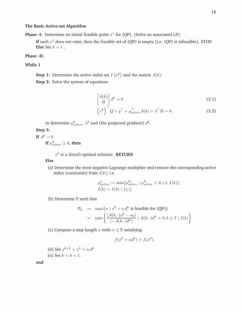
The Basic Active-set Algorithm

Phase -I: Determine an initial feasible point x1 for (QP). (Solve an associated LP).

If such x1 does not exist, then the feasible set of (QP) is empty (i.e. (QP) is infeasible). STOP.

Else Set k = 1 .

Phase -II:

While 1

Step 1: Determine the active index set I(xk

)and the matrix A(k).

Step 2: Solve the system of equations

[A(k)B

]dk = 0 (3.1)

(xk

)⊤

Q+ q⊤ + µ⊤activeA(k) + λ⊤B = 0. (3.2)

to determine µkactive, λk and (the projected gradient) dk.

Step 3:

If dk = 0

If µkactive ≥ 0, then

xk is a (local) optimal solution ,RETURN

Else

(a) Determine the most negative Lagrange multiplier and remove the corresponding active

index (constraint) from I(k); i.e.

µiractive := minµki

active | µki

active < 0, i ∈ I(k)

I(k) = I(k) \ ir.

(b) Determine α such that

αk := maxα | xk + α dk is feasible for (QP)

= min

(A(k, :)xk − a0)

(−A(k, :)dk)| A(k, :)dk < 0, k ∈ I \ I(k)

(c) Compute a step length α with α ≤ α satisfying

f(xk + αdk) < f(xk).

(d) Set xk+1 = xk + α dk

(e) Set k = k + 1.

end

19

Finding Initial Solution for the Active Set method

The active-set algorithm requires an initial feasible point x1. Hence, in Phase-I the following linear

programming problem with artificial variables xn+1, . . . , xn+m+l attached to the constraints of (QP) is

solved:

(LP(QP )) φ(x) :=

m+l∑

i=1

xn+i → min (3.3)

s.t. (3.4)

Ax+

xn+1

...

xn+m

≤ a; (3.5)

Bx+

xn+m+1

...

xn+m+l

= b. (3.6)

If (LP(QP )) has no solution, then (QP) is infeasible. If (LP(QP )) has a solution x1, then we have

φ(x1) = 0. This problem can be solved using linprog.m.

3.1.2 The Interior Reflective Method

The ’LargeScale’, ’on’ option of quadparog.m can be used only when the problem (QP) has simple

bound constraints. When this is the case, quadparog.m uses the interior reflective method of Coleman

and Li to solve (QP). In fact, the interior reflective method also works for non-linear optimization

problems of the form

(NLP ) f(x)→ min

s.t.

lb ≤ x ≤ ub,

where f : Rn → R is a smooth function, lu ∈ R ∪ −∞n and lb ∈ R ∪ ∞n. Thus, for

f(x) = 12x

⊤Qx+ q⊤x, we have a simple bound (QP).

General assumption:

GA1: There is a feasible point that satisfies the bound constraints strictly, i.e.

lb < ub.

Hence, if

F := x ∈ Rn | lb ≤ x ≤ ub

is the feasible set of (NLP), then int(F) = x ∈ Rn | lb < x < ub is non-empty;

GA2: f is at lest twice continuously differentiable;

GA3: for x1 ∈ F , the level set

L := x ∈ F | f(x) ≤ f(x1)

is compact.

20

The Interior Reflective Method (idea):

• generates iterates xk such that

xk ∈ int(F)

using a certain affine (scaling) transformation;

• uses a reflective line search method;

• guarantees global super-linear and local quadratic convergence of the iterates.

The Affine Transformation

We write the problem (NLP) as

(NLP ) f(x)→ min

s.t.

x− ub ≤ 0,

− x+ lb ≤ 0.

Thus, the first order optimality (KKT) conditions at a point x∗ ∈ F will be

∇f(x) + µ1 − µ2 = 0 (3.7)

x− ub ≤ 0 (3.8)

−x+ lb ≤ 0 (3.9)

µ1(x− u) = 0 (3.10)

µ2(−x+ l) = 0 (3.11)

µ1 ≥ 0, µ2 ≥ 0. (3.12)

That is µ1, µ2 ∈ Rn+. For the sake of convenience we also use l and u instead of lb and ub, respectively.

Consequently, the KKT condition can be restated according to the position of the point x in F as

follows:

• if, for some i, li < xi < ui, then the complementarity conditions imply that (∇f(x))i = 0;

• if, for some i, xi = ui, then using (GA1) we have li < xi, thus (µ2)i = 0. Consequently, (∇f(x))i =(µ1)i ⇒ (∇f(x))i ≤ 0.

• if, for some i, xi = li, then using (GA1) we have xi < ui, thus (µ1)i = 0. Consequently, (∇f(x))i =(µ2)i ⇒ (∇f(x))i ≥ 0.

Putting all into one equation we find the equivalent (KKT) condition

(∇f(x))i = 0, if l < xi < ui; (3.13)

(∇f(x))i ≤ 0, if xi = ui; (3.14)

(∇f(x))i ≥ 0, if xi = li. (3.15)

Next define the matrix

D(x) :=

|v1(x)|1/2

. . . |v2(x)|1/2 . . . . . .

. . . . . . . . . . . .. . .

. . . . . . . . . |vn(x)|1/2

=: diag(|v(x)|1/2),

21

where the vector v(x) = (v1(x), . . . , vn(x))⊤ is defined as:

vi := xi − ui, if ∇(f(x))i < 0 and ui <∞;vi := xi − li, if ∇(f(x))i ≥ 0 and li > −∞;vi := −1, if ∇(f(x))i < 0 and ui =∞;vi := 1, if ∇(f(x))i ≥ 0 and li = −∞.

(3.16)

Lemma 3.1.1. A feasible point x satisfies the first order optimality conditions (3.13)-(3.15) iff

D2(x)∇f(x) = 0. (3.17)

Therefore, solving the equation D2(x)∇f(x) = 0 we obtain a point that satisfies the (KKT) condition

for (NLP). Let F (x) := D2(x)∇f(x). Given the iterate xk, to find xk+1 = xk +αkdk, a search direction

dk to solve the problem F (x) = 0 can be obtained by using the Newton method

JF (xk)dk = −F (xk), (3.18)

where JF (·) represents the Jacobian matrix of F (·). It is easy to see that

JF (xk) = D2kHk + diag(∇f(xk))Jv(x

k)

F (xk) = D2(xk)∇f(xk),

where

Hk := ∇2f(xk)

Dk := diag(|v(xk)|1/2)

Jv(xk) :=

∇|v1|

⊤

...

∇|vn|⊤

∈ R

n×n

Remark 3.1.2. Observe that,

(a) since it is assumed that xk ∈ int(F), it follows that |v(xk)| > 0. This implies, the matrixDk = D(xk)is invertible.

(b) due to the definition of the vector v(x), the matrix Jv(x) is a diagonal matrix.

Hence, the system (3.18) can be written in the form(D2

kHk + diag(∇f(xk))Jv(xk)

)dk = −D2

k∇f(xk).

⇒

DkHkDk +D−1

k diag(∇f(xk))Jv(xk)Dk︸ ︷︷ ︸

=diag(∇f(xk))Jv(xk)

D−1

k dk = −Dk∇f(xk)

⇒(DkHkDk + diag(∇f(xk))Jv(x

k))D−1

k dk = −Dk∇f(xk).

Now define

xk := D−1k xk

dk := D−1k dk

Bk := DkHkDk + diag(∇f(xk))Jv(xk)

gk := Dk∇f(xk),

22

where xk = D−1k xk defines an affine transformation of the variables x into x using D(x). In general,

we can also write B(x) := D(x)H(x)D(x) + diag(∇f(x))Jv(x) and g(x) = D(x)∇f(x). Hence, the

system (3.18) will be the same as

Bkdk = −gk.

Lemma 3.1.3. Let x∗ ∈ F .

(i) If x∗ is a local minimizer of (NLP), then g(x∗) = 0;

(ii) If x∗ is a local minimizer of (NLP), then B(x∗) is positive definite and g(x∗) = 0;

(iii) If B(x∗) is positive definite and g(x∗) = 0, then x∗ is a local minimizer of (NLP).

Remark 3.1.4. Thus statements (i) and (ii) of Lem. 3.1.3 imply that

x∗ is a solution of (NLP) ⇔ g(x∗) = 0 and B(x∗) is positive definite.

It follows that, through the affine transformation x = D−1x, the problem (NLP) has been transformed

into an unconstrained minimization problem with gradient vector g and Hessian matrix B. Consequently,

a local quadratic model for the transformed problem can be given by the trust region problem:

(QP )TR ψ(s) =1

2sBks+ g⊤k s→ min,

s.t.

‖s‖ ≤ k.

Furthermore, the system Bkdk = −gk can be considered as the first order optimality condition (considering

dk as a local optimal point) for the unconstrained problem (QP)TR with ‖dk‖ < k.

Retransforming variables the problem (QP )TR

1

2s[DkHkDk + diag(∇f(xk))Jv(x

k)]s+ (Dk∇f(xk))⊤s→ min,

s.t.

‖s‖ ≤ k.

⇒

1

2sDk[Hk +D−1

k diag(∇f(xk))Jv(xk)D−1

k ]Dks+ f(xk)⊤Dks→ min,

s.t.

‖s‖ ≤ k.

with s = Dks and

Bk := Hk +D−1k diag(∇f(xk))Jv(x

k)D−1k

we obtain the following quadratic problem in terms of the original variables

(QP )TRO1

2sBks+∇f(xk)⊤s→ min,

s.t.

‖D−1k s‖ ≤ k.

Consequently, given xk the problem (QP)TRO is solved to determine sk so that

xk+1 = xk + αksk,

for some step length αk.

23

Reflective Line Search

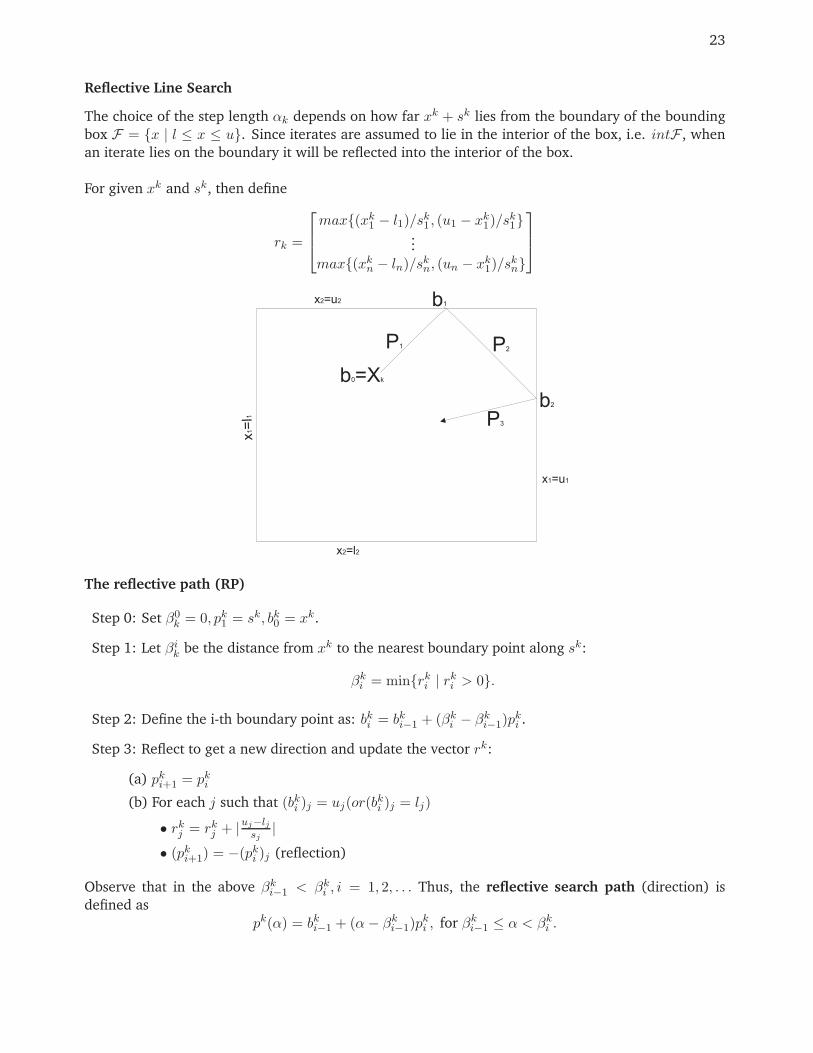
The choice of the step length αk depends on how far xk + sk lies from the boundary of the bounding

box F = x | l ≤ x ≤ u. Since iterates are assumed to lie in the interior of the box, i.e. intF , when

an iterate lies on the boundary it will be reflected into the interior of the box.

For given xk and sk, then define

rk =

max(xk

1 − l1)/sk1 , (u1 − x

k1)/s

k1

...

max(xkn − ln)/sk

n, (un − xk1)/s

kn

b =X0 k

P1

b1

b2

P2

P3

x =l2 2

x=

l1

1

x =u2 2

x =u1 1

The reflective path (RP)

Step 0: Set β0k = 0, pk

1 = sk, bk0 = xk.

Step 1: Let βik be the distance from xk to the nearest boundary point along sk:

βki = minrk

i | rki > 0.

Step 2: Define the i-th boundary point as: bki = bki−1 + (βki − β

ki−1)p

ki .

Step 3: Reflect to get a new direction and update the vector rk:

(a) pki+1 = pk

i

(b) For each j such that (bki )j = uj(or(bki )j = lj)

• rkj = rk

j + |uj−lj

sj|

• (pki+1) = −(pk

i )j (reflection)

Observe that in the above βki−1 < βk

i , i = 1, 2, . . . Thus, the reflective search path (direction) is

defined as

pk(α) = bki−1 + (α− βki−1)p

ki , for βk

i−1 ≤ α < βki .

24

The interior-reflective method (TIR)

Step 1: Choose x1 ∈ int(F).

Step 2: Determine a descent direction sk for f at xk ∈ int(F). Then determine the reflective search

path pk(α) using the algorithm (RP).

Step 2: Solve f(xk + pk(α))→ min to determine αk in such a way that xk + pk(αk) is not a boundary

point of F .

Step 3: xk+1 = xk + pk(αk).

Under additional assumptions, the algorithm (TIR) has a global super-linear and local quadratic con-

vergence properties. For details see the papers of Coleman & Li ([1] - [3]).

Multiple image restoration and enhancement

3.2 Using quadprog to Solve QP Problems

3.2.1 Theoretical Problems

1. Solve the following quadratic optimization by using quadprog.m

x21 + 2x2

2+ 2x1+ 3x2 → mins.t.

x1+ 2x2 ≤ 82x1+ x2 ≤ 10

x2 ≤ 3x1, x2 ≥ 0

Soution:

Q =

(2 00 4

), q =

(23

), A =

1 22 10 1

, a =

8103

, B = [ ], b = [ ], lb =

(00

), ub =

(∞∞

)

Matlab Solution

function QpEx1

Q=[2,0;0,4]; q=[2,3]’; A=[1,2;2,1;0,1]; a=[8,10,3];"

lb=[0,0]’; ub=[inf;inf];

options=optimset(’quadprog’);

options=optimset(’LargeScale’,’off’);

[xsol,fsolve,exitflag,output]=QUADPROG(Q,q,A,a,[],[],lb,ub,[],options);

25

fprintf(’%s ’,’Convergence: ’)

if exitflag > 0

fprintf(’%s \n’,’Ja!’);

disp(’Solution obtained:’)

xsol

else

fprintf(’%s \n’,’Non convergence!’);

end

fprintf(’%s %s \n’,’Algorithm used: ’,output.algorithm)

x=[-3:0.1:3]; y=[-4:0.1:4]; [X,Y]=meshgrid(x,y);

Z=X.^2+2*Y.^2+2*X+3*Y; meshc(X,Y,Z); hold on

plot(xsol(1),xsol(2),’r*’)

2. Solve the following (QP) using quadprog.m

x21 + x1x2 + 2x2

2 +2x23 +2x2x3 +4x1+ 6x2 +12x3 → min

s.t.

x1 +x2 +x3 ≥ 6−x1 −x2 +2x3 ≥ 2x1, x2 x3 ≥ 0

Soution:

Q =

2 1 01 4 20 2 4

, q =

4612

, A =

(−1 −1 −11 1 −2

), a =

(−6−12

),

B = [ ], b = [ ], lb =

000

, ub =

∞∞∞

Matlab Solution

function QpEx2

Q=[2,1,0;1,4,2;0,2,4]; q=[4,6,12]; A=[-1,-1,-1;1,2,-2]; a=[-6,-2];

lb=[0;0;0]’; ub=[inf;inf;inf];

options=optimset(’quadprog’);

options=optimset(’LargeScale’,’off’);

[xsol,fsolve,exitflag,output]=QUADPROG(Q,q,A,a,[],[],lb,ub,[],options);

fprintf(’%s ’,’Convergence: ’)

if exitflag > 0

26

fprintf(’%s \n’,’Ja!’);

disp(’Solution obtained:’)

xsol

else

fprintf(’%s \n’,’Non convergence!’);

end

fprintf(’%s %s \n’,’Algorithm used: ’,output.algorithm)

3.2.2 Production model - profit maximization

Let us consider the following production model. A factory produces n− articles Ai ,i = 1, 2, ..., n, The

cost function c (x) for the production process of the articles can be desribed by

c (x) = kTp x+ kf + km (x)

where kp, kf and km denote the variable production cost rates, the fix costs and the variable costs for

the material. Further assume that the price p of a product depends on the number of products x in

some linear relation

pi = ai − bixi, ai , bi > 0, i = 1, 2, ..., n

The profit Φ (x) is given as the difference of the turnover

T (x) = p (x)T xT =

n∑

i=1

(aixi − bix

2i

)

and the costs c (x) . Hence

Φ (x) =

n∑

i=1

(aixi − bix

2i

)−

(kT

p x+ kf + km (x))

=1

2xT

−2b1 0 · · · 00 −2b2 · · · 0...

.... . .

...

0 0 · · · −2bn

︸ ︷︷ ︸:=B

x+ (a− kp)T x− kf − km (x)

Further we have the natural constraints

ai − bixi ≥ 0, i = 1, 2, ..., n ⇒

b1 0 . . . 00 . . . 0...

. . ....

0 . . . 0 bn

︸ ︷︷ ︸B′

x ≤ a

kTp x+ kf ≤ k0

0 < xmin ≤ x ≤ xmax

and constraints additional constraints on resources. There are resources Bj, j = 1, . . . ,m with con-

sumption amount yj, j = 1, 2, ...,m. Then the y′js and the amount of final products xi have the linear

connection

y = Rx

27

Further we have some bounds

0 < ymin ≤ y ≤ ymax

based on the minimum resource consumption and maximum available resources. When we buy re-

sources Bj we have to pay the following prices for yj units of Bj

(cj − djyj) yj, j = 1, 2, ...,m

which yields the cost function

km (x) =

m∑

j=1

(cj − djyj) yj

= cT y +1

2yT

−2d1 0 · · · 00 −2d2 · · · 0...

.... . .

...

0 0 · · · −2dm

y

= cTRx+1

2xTRT

−2d1 0 · · · 00 −2d2 · · · 0...

.... . .

...

0 0 · · · −2dm

︸ ︷︷ ︸:=D

Rx

We assume some production constraints given by

Ax ≤ r

Bx ≥ s.

If we want to maximize the profit (or minimize loss) we get the following quadratic problem

1

2x⊤

(B +R⊤DR

)x+ (a− kp +R⊤c)⊤x− kf → max

s.t.

B′x ≤ a

k⊤p x ≤ k0 − kf

Rx ≥ ymin

Rx ≤ ymax

Ax ≤ r

Bx ≥ s

0 < xmin ≤ x ≤ xmax.

Use hypothetical, but properly chosen, data for A,B,R,a,b,c,d,r,s,xmin,xmax,kp,k0,kf to run the follow-

ing program to solve the above profit maximization problem.

function [xsol,fsolve,exitflag,output]=profit(A,B,R,a,b,c,d,r,s,xmin,xmax,kp,k0,kf)

%[xsol,fsolve,exitflag,output]=profit(A,B,R,a,b,c,d,r,s,xmin,xmax,kp,k0,kf)

%solves a profit maximization prblem

28

Bt=-2*diag(b); D=-2*diag(d);

%%1/2x’Qx + q’x

Q=Bt + R’*D*R; q=a-kp+R’*c;

%coefficeint matrix of inequality constraints

A=[diag(b);kp’;-R;R;A;-B];

%right hand-side vector of inequality constraints

a=[a;k0-kf;-ymin;ymax;r;-s];

%Bound constraints

lb=xmin(:); ub=xmax(:);

%Call quadprog.m to solve the problem

options=optimset(’quadprog’);

options=optimset(’LargeScale’,’off’);

[xsol,fsolve,exitflag,output]=quadprog(-Q,-q,A,a,[],[],lb,ub,[],options);

Bibliography

[1] T. F. Coleman, Y. Li: On the convergence of interior-reflective Newton methods for non-linear

optimization subjecto to bounds. Math. Prog., V. 67, pp. 189-224, 1994.

[2] T. F. Coleman, Y. Li: A reflective Newton method for minimizing a quadratic function subject to

bounds on some of the variables. SIAM Journal on Optimization, Volume 6 , pp. 1040 - 1058,

1996.

[3] T. F. Coleman, Y. Li: An interior trust region approach for nonlinear optimization subject to

bounds. SIAM Journal on Optimization, SIAM Journal on Optimization, V. 6, pp. 418-445, 1996.

29

Chapter 4

Unconstrained nonlinear programming

4.1 Theory, optimality conditions

4.1.1 Problems, assumptions, definitions

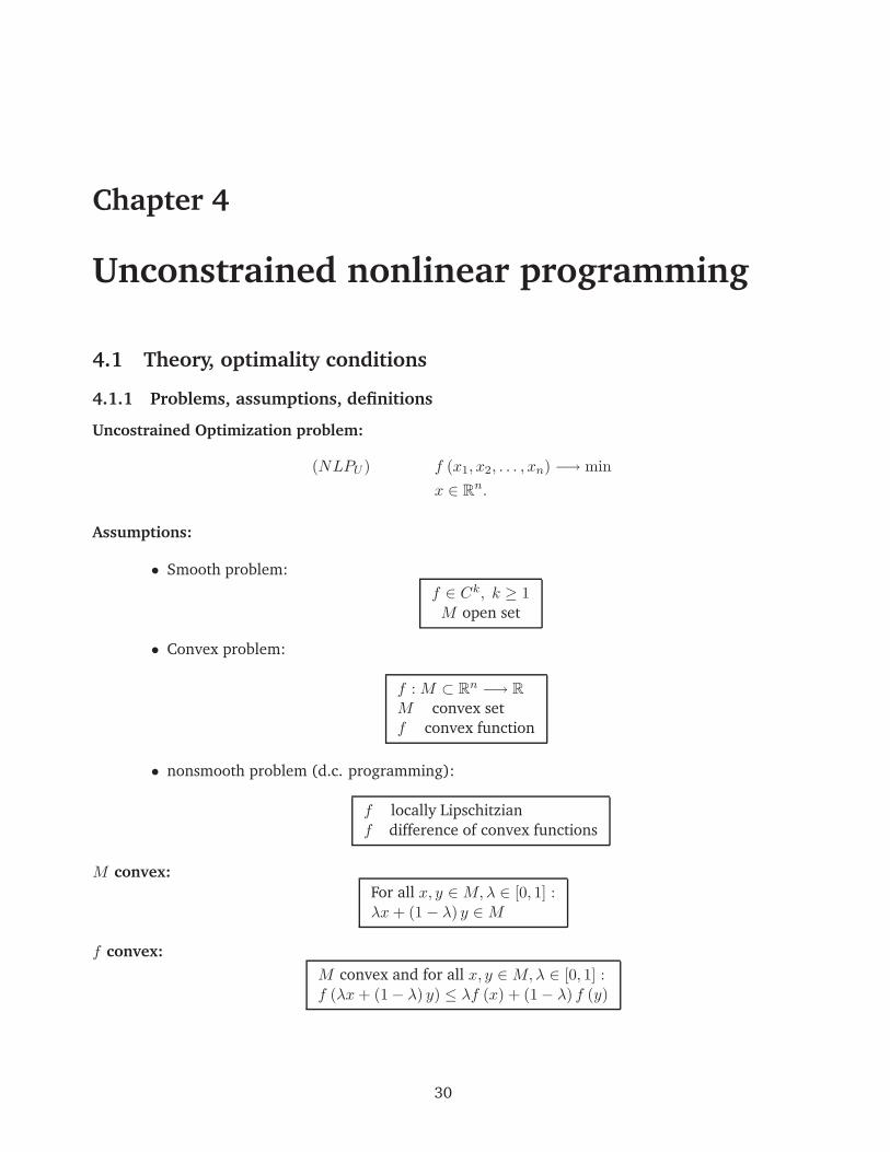
Uncostrained Optimization problem:

(NLPU ) f (x1, x2, . . . , xn) −→ min

x ∈ Rn.

Assumptions:

• Smooth problem:

f ∈ Ck, k ≥ 1M open set

• Convex problem:

f : M ⊂ Rn −→ R

M convex set

f convex function

• nonsmooth problem (d.c. programming):

f locally Lipschitzian

f difference of convex functions

M convex:

For all x, y ∈M,λ ∈ [0, 1] :λx+ (1− λ) y ∈M

f convex:

M convex and for all x, y ∈M,λ ∈ [0, 1] :f (λx+ (1− λ) y) ≤ λf (x) + (1− λ) f (y)

30

31

f Lipschitzian:

There is a K ≥ 0 such that for all x, y ∈M :|f (x)− f (y)| ≤ K ‖x− y‖

‖x− y‖ =

√(x− y)T (x− y)

Locally Lipschitzian: If, for any x ∈ M , there is a ball B (x) around x and a constant K such that fis Lipschitzian on M ∩B.

4.2 Optimality conditions for smooth unconstrained problems

Necessary condition: Assumption f ∈ C1

f has a local minimum at x ∈M

⇐⇒ There is a ball B around x such that

f(x) ≤ f(x) for all x ∈M ∩B(x)

=⇒∂

∂xkf (x) = 0, k = 1, 2, ..., n

Sufficient condition: Assumption f ∈ C2

(1)∂

∂xkf (x) = 0, k = 1, 2, ..., n

(2) Hf (x) = ∇2f (x) =

(∂2

∂xj∂xkf (x)

)

nnis positively definite

=⇒ f has a strict local minimum at x ∈M

Remark: A symmetric Matrix H is positively definite⇐⇒ all eigenvalues of H are greater than zero.

MATLAB call:

λ = eig (H)

computes all eigenvalues of the Matrix H and stores them in the vector λ.

Saddle point: Assumption f ∈ C2

(1)∂

∂xkf (x) = 0, k = 1, 2, ..., n

(2) Hf (x) = ∇2f (x) =

(∂2

∂xj∂xkf (x)

)

nnhas only nonzero eigenvalues but at least two

with different sign

=⇒ f has a saddle point at x ∈M

32

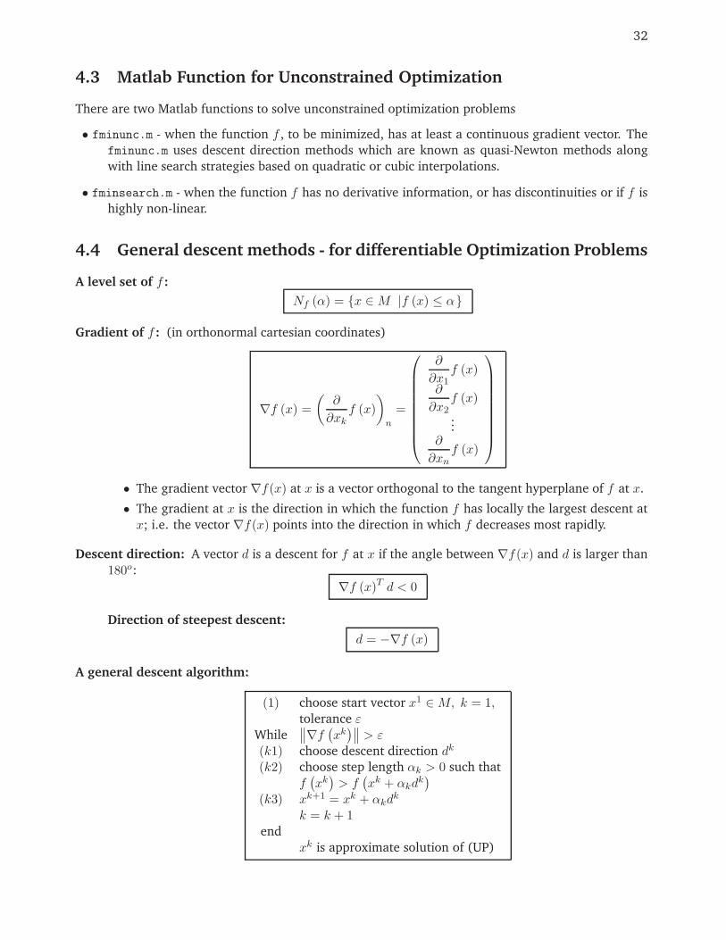
4.3 Matlab Function for Unconstrained Optimization

There are two Matlab functions to solve unconstrained optimization problems

• fminunc.m - when the function f , to be minimized, has at least a continuous gradient vector. The

fminunc.m uses descent direction methods which are known as quasi-Newton methods along

with line search strategies based on quadratic or cubic interpolations.

• fminsearch.m - when the function f has no derivative information, or has discontinuities or if f is

highly non-linear.

4.4 General descent methods - for differentiable Optimization Problems

A level set of f :

Nf (α) = x ∈M |f (x) ≤ α

Gradient of f : (in orthonormal cartesian coordinates)

∇f (x) =

(∂

∂xkf (x)

)

n

=

∂

∂x1f (x)

∂

∂x2f (x)

...∂

∂xnf (x)

• The gradient vector ∇f(x) at x is a vector orthogonal to the tangent hyperplane of f at x.

• The gradient at x is the direction in which the function f has locally the largest descent at

x; i.e. the vector ∇f(x) points into the direction in which f decreases most rapidly.

Descent direction: A vector d is a descent for f at x if the angle between ∇f(x) and d is larger than

180o:

∇f (x)T d < 0

Direction of steepest descent:

d = −∇f (x)

A general descent algorithm:

(1) choose start vector x1 ∈M, k = 1,tolerance ε

While∥∥∇f

(xk

)∥∥ > ε(k1) choose descent direction dk

(k2) choose step length αk > 0 such that

f(xk

)> f

(xk + αkd

k)

(k3) xk+1 = xk + αkdk

k = k + 1end

xk is approximate solution of (UP)

33

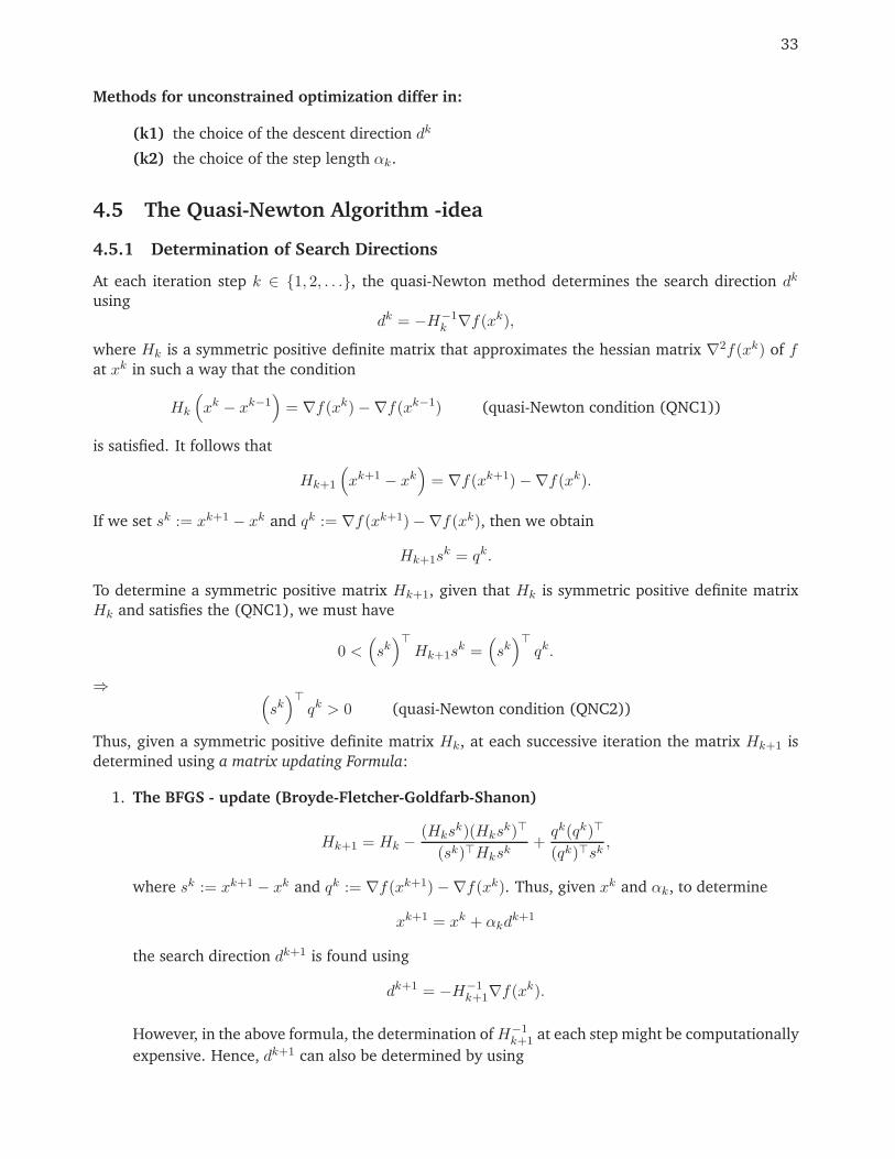
Methods for unconstrained optimization differ in:

(k1) the choice of the descent direction dk

(k2) the choice of the step length αk.

4.5 The Quasi-Newton Algorithm -idea

4.5.1 Determination of Search Directions

At each iteration step k ∈ 1, 2, . . ., the quasi-Newton method determines the search direction dk

using

dk = −H−1k ∇f(xk),

where Hk is a symmetric positive definite matrix that approximates the hessian matrix ∇2f(xk) of fat xk in such a way that the condition

Hk

(xk − xk−1

)= ∇f(xk)−∇f(xk−1) (quasi-Newton condition (QNC1))

is satisfied. It follows that

Hk+1

(xk+1 − xk

)= ∇f(xk+1)−∇f(xk).

If we set sk := xk+1 − xk and qk := ∇f(xk+1)−∇f(xk), then we obtain

Hk+1sk = qk.

To determine a symmetric positive matrix Hk+1, given that Hk is symmetric positive definite matrix

Hk and satisfies the (QNC1), we must have

0 <(sk

)⊤

Hk+1sk =

(sk

)⊤

qk.

⇒ (sk

)⊤

qk > 0 (quasi-Newton condition (QNC2))

Thus, given a symmetric positive definite matrix Hk, at each successive iteration the matrix Hk+1 is

determined using a matrix updating Formula:

1. The BFGS - update (Broyde-Fletcher-Goldfarb-Shanon)

Hk+1 = Hk −(Hks

k)(Hksk)⊤

(sk)⊤Hksk+qk(qk)⊤

(qk)⊤sk,

where sk := xk+1 − xk and qk := ∇f(xk+1)−∇f(xk). Thus, given xk and αk, to determine

xk+1 = xk + αkdk+1

the search direction dk+1 is found using

dk+1 = −H−1k+1∇f(xk).

However, in the above formula, the determination ofH−1k+1 at each step might be computationally

expensive. Hence, dk+1 can also be determined by using

34

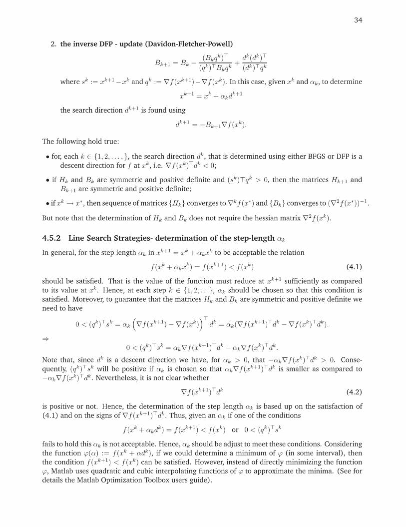
2. the inverse DFP - update (Davidon-Fletcher-Powell)

Bk+1 = Bk −(Bkq

k)⊤

(qk)⊤Bkqk+dk(dk)⊤

(dk)⊤qk

where sk := xk+1−xk and qk := ∇f(xk+1)−∇f(xk). In this case, given xk and αk, to determine

xk+1 = xk + αkdk+1

the search direction dk+1 is found using

dk+1 = −Bk+1∇f(xk).

The following hold true:

• for, each k ∈ 1, 2, . . . , , the search direction dk, that is determined using either BFGS or DFP is a

descent direction for f at xk, i.e. ∇f(xk)⊤dk < 0;

• if Hk and Bk are symmetric and positive definite and (sk)⊤qk > 0, then the matrices Hk+1 and

Bk+1 are symmetric and positive definite;

• if xk → x∗, then sequence of matrices Hk converges to∇kf(x∗) and Bk converges to (∇2f(x∗))−1.

But note that the determination of Hk and Bk does not require the hessian matrix ∇2f(xk).

4.5.2 Line Search Strategies- determination of the step-length αk

In general, for the step length αk in xk+1 = xk + αkxk to be acceptable the relation

f(xk + αkxk) = f(xk+1) < f(xk) (4.1)

should be satisfied. That is the value of the function must reduce at xk+1 sufficiently as compared

to its value at xk. Hence, at each step k ∈ 1, 2, . . ., αk should be chosen so that this condition is

satisfied. Moreover, to guarantee that the matrices Hk and Bk are symmetric and positive definite we

need to have

0 < (qk)⊤sk = αk

(∇f(xk+1)−∇f(xk)

)⊤

dk = αk(∇f(xk+1)⊤dk −∇f(xk)⊤dk).

⇒0 < (qk)⊤sk = αk∇f(xk+1)⊤dk − αk∇f(xk)⊤dk.

Note that, since dk is a descent direction we have, for αk > 0, that −αk∇f(xk)⊤dk > 0. Conse-

quently, (qk)⊤sk will be positive if αk is chosen so that αk∇f(xk+1)⊤dk is smaller as compared to

−αk∇f(xk)⊤dk. Nevertheless, it is not clear whether

∇f(xk+1)⊤dk (4.2)

is positive or not. Hence, the determination of the step length αk is based up on the satisfaction of

(4.1) and on the signs of ∇f(xk+1)⊤dk. Thus, given an αk if one of the conditions

f(xk + αkdk) = f(xk+1) < f(xk) or 0 < (qk)⊤sk

fails to hold this αk is not acceptable. Hence, αk should be adjust to meet these conditions. Considering

the function ϕ(α) := f(xk + αdk), if we could determine a minimum of ϕ (in some interval), then

the condition f(xk+1) < f(xk) can be satisfied. However, instead of directly minimizing the function

ϕ, Matlab uses quadratic and cubic interpolating functions of ϕ to approximate the minima. (See for

details the Matlab Optimization Toolbox users guide).

35

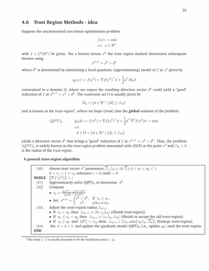
4.6 Trust Region Methods - idea

Suppose the unconstrained non-linear optimization problem

f(x)→ min

s.t. x ∈ Rn

with f ∈ C2(Rn) be given. For a known iterate xk the trust region method determines subsequent

iterates using

xk+1 = xk + dk

where dk is determined by minimizing a local quadratic (approximating) model of f at xk given by

qk(x) := f(xk) +∇f(xk)⊤d+1

2d⊤Hkd

constrained to a domain Ω, where we expect the resulting direction vector dk could yield a "good"

reduction of f at xk+1 = xk + dk. The constraint set Ω is usually given by

Ωk = d ∈ Rn | ‖d‖ ≤ k

and is known as the trust-region1, where we hope (trust) that the global solution of the problem

(QPT )k qk(d) := f(xk) +∇f(xk)⊤d+1

2d⊤∇2f(xk)d→ min

s.t.

d ∈ Ω = d ∈ Rn | ‖d‖ ≤ k

yields a direction vector dk that brings a "good" reduction of f at xk+1 = xk + dk. Thus, the problem

(QPT )k is widely known as the trust region problem associated with (NLP) at the point xk andk > 0is the radius of the trust-region.

A general trust-region algorithm

(k0) choose start vector x0 parameters ,0 ∈ (0,), 0 < η1 ≤ η2 < 10 < γ1 < 1 < γ2, tolerance ε > 0, andk = 0.

WHILE∥∥∇f

(xk

)∥∥ > ε(k1) Approximately solve (QPT)k to determine dk.(k2) Compute

• rk = f(xk) − f(xk+dk)qk(0) − qk(dk)

• Set xk+1 =

xk + dk, if rk ≥ η1,xk, otherwise.

(k3) Adjust the trust-region radius k+1

• If rk < η1, then k+1 :∈ (0, γ1k) (Shrink trust-region).

• If η1 ≤ rk < η2, then k+1 ∈ [γ1k,k] (Shrink or accept the old trust-region).

• If rk ≥ η2 and ‖dk‖ = k, then k+1 ∈ [k,minγ2k,k] (Enlarge trust-region).

(k4) Set k = k + 1 and update the quadratic model (QPT)k; i.e., update qk(·)and the trust-region.END

1The norm ‖ · ‖ is usually assumed to be the Euclidean norm ‖ · ‖2.

36

In the above algorithm the parameter is the overall bound for the trust region radius k and the

expression:

rk =f(xk) − f(xk + dk)

qk(0) − qk(dk)

measures how best the quadratic model approximates the unconstrained problem (NLP). Thus,

• aredk := f(xk)− f(xk + dk) is known as the actual reduction of f at step k + 1; and

• predk := qk(0) − q(dk) is the predicted reduction of f achievable through the approximating model

(QPT)k at step k + 1.

Consequently, rk measures the ratio of the actual reduction to the predicted reduction. Hence, at step

k + 1,

• if rk ≥ η2, then this step is called a very successful step. Accordingly, the trust-region will be

enlarged; i.e. k+1 ≥ k. In particular, a sufficient reduction of f will be achieved through the

model, since

f(xk) − f(xk + dk) ≥ η2(qk(0) − qk(dk)) > 0.

• if rk ≥ η1, then this step is called a successful step since

f(xk) − f(xk + dk) ≥ η1(qk(0) − qk(dk)) > 0.

Accordingly, the search direction is accepted, for it brings a sufficient decrease in the value of f ;

i.e. xk+1 = xk + dk and the trust-region can remain as it is for the next step.

• However, if rk < η1, then the step is called unsuccessful. That is the direction dk does not provide

a sufficient reduction of f . This is perhaps due to a too big trust-region (i.e. at this step the

model (QPT)k is not trustworthy). Consequently, dk will be rejected and so xk+1 = xk and for

the next step the trust-region radius will be reduced.

Note, that in general, if rk ≥ η1 or rk ≥ η2, then xk+1 = xk + dk and the corresponding step is

successful. In any case, the very important issue in a trust-region algorithm is how to solve the trust-

region sub-problem (QPT)k.

4.6.1 Solution of the Trust-Region Sub-problem

Remark 4.6.1. Considering the trust-region sub-problem (QPT)k:

• since, for each k, qk(·) is a continuous function and Ω = d ∈ Rn | ‖d‖ ≤ k is a compact set, the

problem (QPT)k has always a solution.

• Furthermore, if f is not a convex function, then the hessian matrix ∇2f(xk) of f at xk may not be

positive definite. Thus, the global solution of (QPT)k may not exist.

The existence of a global solution for (QPT)k is guaranteed by the following statement:

Theorem 4.6.2 (Thm. 2.1. [3], Lem. 2.8. [10], also [4]).

Given a quadratic optimization problem

(QP ) q(d) := f + g⊤d+1

2d⊤Hd→ min

s.t.

d ∈ Ω = d ∈ Rn | ‖d‖ ≤

with f ∈ R, g ∈ Rn and H a symmetric matrix and > 0. Then d∗ ∈ R

n is a global solution of (QP) if

and only if, there is a (unique) λ∗ such that

37

(a) λ∗ ≥ 0, ‖d∗‖ ≤ and λ∗(‖d∗‖ −) = 0;

(b) (H + λ∗I)d∗ = −g and (H + λ∗I) is positive definite;

where I is the identity matrix.

The statements of Thm. 4.6.2 describe the optimality conditions of dk as a solution of the trust-region

sub-problem (QPTR)k. Hence, the choice of dk is based on whether the matrix Hk = ∇2f(xk) is

positive definite or not.

Remark 4.6.3. Note that,

(i) if H is a positive definite matrix and ‖H−1k gk‖ < , then for the solution of d∗ of (QP), ‖dk‖ =

does note hold; i.e., in this case the solution of (QP) does not lie on the boundary of the feasible set.

Assume that Hk is a positive definite, ‖H−1k g‖ < and ‖dk‖ = hold at the same time. Hence,

from Thm. 4.6.2(b), we have that

(I + λ∗H−1k )d∗ = −H−1

k gk ⇒ dk⊤d∗ + λkdk⊤H−1

k dk = −dk⊤H−1k gk,

where gk := ∇f(xk). By the positive definiteness of H−1 we have

dk⊤dk +λk

maxEig(Hk)dk⊤dk ≤ −dk⊤H−1

k gk

⇒ (1 +

λk

maxEig(Hk)

)‖dk‖2 ≤ ‖ − dk⊤‖‖H−1

k gk‖ < ‖dk‖ = ‖dk‖2,

where maxEig(Hk) is the largest eigenvalue of H. Hence,(1 + λk

maxEig(Hk)

)‖dk‖2 < ‖dk‖2. But

this is a contradiction, since λk ≥ 0.

(ii) Conversely, if (QP) has a solution d∗ such that ‖dk‖ < , it follows that λk = 0 and Hk is positive

definite. Obviously, from Thm. 4.6.2(a), we have λk = 0. Consequently, Hk + λkI is positive

definite, implies that Hk is positive definite.

In general, if Hk is positive definite, then H + λ∗I is also positive definite.

The Matlab trust-region algorithm tries to find a search direction dk in a two-dimensional subspace of

Rn. Thus, the trust-region sub-problem has the form:

(QPT )k qk(d) := f(xk) + g⊤k d+1

2d⊤Hkd→ min

s.t.

d ∈ Ω = d ∈ Rn | ‖d‖ ≤ k, d ∈ Sk,

where S is a two-dimensional subspace of Rn; i.e. Sk =< uk, vk >; with u, v ∈ R

n. This approach

reduces computational costs of when solving large scale problems [?]. Thus, the solution algorithm

for (QPT)k chooses an appropriate two-dimensional subspace at each iteration step.

Case -1: If Hk is positive definite, then

Sk =⟨gk,−H

−1k gk

⟩

38

Case -2 : If Hk is not positive definite, then

Sk = 〈gk, uk〉

such that

Case - 2a: either uk satisfies

Hkuk = −gk;

Case - 2b: or uk is chosen as a direction of negative-curvature of f at xk; i.e.

u⊤k Hkuk < 0.

Remark 4.6.4. Considering the case whenHk is not positive definite, we make the following observations.

(i) If the Hk has negative eigenvalues, then let λk1 be the smallest negative eigenvalue and wk be the

corresponding eigenvector . Hence, we have

Hkwk = λ1wk ⇒ w⊤

k Hkwk = λk1‖wk‖

2 < 0.

satisfying Case 2a. Furthermore,

(Hk + (−λk1)I)wk = 0.

Since wk 6= 0, it follows that (Hk +(−λk1)I) is not positive definite. Hence, in the Case 2a, the vector

uk can be chosen to be equal to wk. Furthermore, the matrix (Hk + (−λk1)I) is also not positive

definite.

(ii) If all eigenvalues of Hk are equal to zero, then

(iia) if gk is orthogonal to the null-space of Hk, then there is a vector uk such that

Hkuk = −gk.

This follows from the fact that Hk is a symmetric matrix and Rn = N (Hk)

⊕R(Hk)

2.

(iia) Otherwise, there is always a non-zero vector uk 6= 0 such that u⊤k Hkuk ≤ 0.

(iii) The advantage of using a direction of negative curvature is to avoid the convergence of the algorithm

to a saddle point or a maximizer of (QPTR)k

A detailed discussion of the algorithms for the solution of the trust-region quadratic sub-problem

(QPT)k are found in the papers [1, 9] in the recent book of Conn et al. [2].

4.6.2 The Trust Sub-Problem under Considered in the Matlab Optimization toolbox

The Matlab routine fminunc.m attempts to determine the search direction dk by solving a trust-region

quadratic sub-problem on a two dimensional sub-space Sk of the following form :

(QPT2)k qk(d) := ∇g⊤k d+1

2d⊤Hkd→ min

s.t.

d ∈ Ω = d ∈ Rn | ‖Dd‖ ≤ k, d ∈ Sk,

where dim(Sk) = 2 and D is a non-singular diagonal scaling matrix.

2N (Hk)⊕

R(Hk) represents the direct-sum of the null- and range -spaces of Hk.

39

The scaling matrix D is usually chosen to guarantee the well-posedness of the problem. For this

problem the optimality condition given in Thm. 4.6.2 can be stated as

(Hk + λkD⊤D)dk = −gk.

At the same time, the parameter λk can be thought of as having a regularizing effect in case of

ill-posedness. However, if we use the variable transformation s = Dd we obtain that

(QPT2)k qk(s) := ∇g⊤k (D−1s) +1

2(D−1s)⊤Hk(D

−1s)→ min

s.t.

d ∈ Ω = d ∈ Rn | ‖s‖ ≤ k,D

−1s ∈ Sk,

But this is the same as

(QPT2)k qk(s) := ∇g⊤k s+1

2s⊤Hks→ min

s.t.

d ∈ Ω = d ∈ Rn | ‖s‖ ≤ k,D

−1s ∈ Sk,

where gk := D−1gk and Hk := D−1HkDk. The approach described in Sec. 4.6.1 can be used to

solve (QPT2)k without posing any theoretical or computational difficulty. For a discussion of problem

(QPT2)k with a general non-singular matrix D see Gay [3].

4.6.3 Calling and Using fminunc.m to Solve Unconstrained Problems

[xsol,fopt,exitflag,output,grad,hessian] = fminunc(fun,x0,options)

Input arguments:

fun a Matlab function m-file that contains the function to be minimzed

x0 Startvector for the algorithm, if known, else [ ]

options options are set using the optimset funciton, they determine what algorism to use,etc.

Output arguments:

xsol optimal solution

fopt optimal value of the objective function; i.e. f(xopt)

exitflag tells whether the algorithm converged or not, exitflag > 0 means convergence

output a struct for number of iterations, algorithm used and PCG iterations(when LargeScale=on)

grad gradient vector at the optimal point xsol.

hessian hessian matrix at the optimal point xsol.

To display the type of options that are available and can be used with the fminunc.m use

>>optimset(’fminunc’)

Hence, from the list of option parameters displayed, you can easily see that some of them have default

values. However, you can adjust these values depending on the type of problem you want to solve.

However, when you change the default values of some of the parameters, Matlab might adjust other

parameters automatically.

As for quadprog.m there are two types of algorithms that you can use with fminunc.m

40

(i) Medium-scale algorithms: The medium-scale algorithms under fminunc.m are based on the

Quasi-Newton method. This options used to solve problems of smaller dimensions. As usual

this is set using

>>OldOptions=optimset(’fminunc’);

>>Options=optimset(OldOptions,’LargeScale’,’off’);

With medium Scale algorithm you can also decide how the search direction dk be determined by

adjusting the parameter HessUpdate by using one of:

>>Options=optimset(OldOptions,’LargeScale’,’off’,’HessUpdate’,’bfgs’);

>>Options=optimset(OldOptions,’LargeScale’,’off’,’HessUpdate’,’dfp’);

>>Options=optimset(OldOptions,’LargeScale’,’off’,’HessUpdate’,’steepdesc’);

(ii) Large-scale algorithms: By default the LargeScale option parameter of Matlab is always on.

However, you can set it using

>>OldOptions=optimset(’fminunc’);

>>Options=optimset(OldOptions,’LargeScale’,’on’);

When the ’LargeScale’ is set ’on’, then fminunc.m solves the given unconstrained problem using

the trust-region method. Usually, the large-scale option of fminunc is used to solve problems

with very large number of variables or with sparse hessian matrices. Such problem, for instance,

might arise from discretized optimal control problems, some inverse-problems in signal process-

ing etc.

However, to use the large-scale algorithm under fminunc.m, the gradient of the objective function

must be provided by the user and the parameter ’GradObj’ must be set ’on’ using:

>>Options=optimset(OldOptions,’LargeScale’,’on’,’GradObj’,’on’);

Hence, for the large-scale option, you can define your objective and gradient functions in a single

function m-file :

function [fun,grad]=myFun(x)

fun = ...;

if nargout > 1

grad = ...;

end

However, if you fail to provide the gradient of the objective function, then fminunc uses the

medium-scale algorithm to solve the problem.

Experiment: Write programs to solve the following problem with fminunc.m using both the medium-

and large-scale options and compare the results.

f(x) = x21 + 3x2

2 + 5x23 → min

x ∈ Rn.

Solution

41

Define the problem in an m-file, including the derivative in case if you want to use the LargeSclae

option.

function [f,g]=fun1(x)

%Objective function for example (a)

%Defines an unconstrained optimization problem to be solved with fminunc

f=x(1)^2+3*x(2)^2+5*x(3)^2;

if nargout > 1

g(1)=2*x(1);

g(2)=6*x(2);

g(3)=10*x(3);

end

Next you can write a Matlab m-file to call fminunc to solve the problem.

function [xopt,fopt,exitflag]=unConstEx1

options=optimset(’fminunc’);

options.LargeScale=’off’; options.HessUpdate=’bfgs’;

%assuming the function is defined in the

%in the m file fun1.m we call fminunc

%with a starting point x0

x0=[1,1,1];

[xopt,fopt,exitflag]=fminunc(@fun1,x0,options);

If you decide to use the Large-Scale algorithm on the problem, then you need to simply change

the option parameter LargeScale to on.

function [xopt,fopt,exitflag]=unConstEx1

options=optimset(’fminunc’);

options.LargeScale=’on’;

options.Gradobj=’on’;

%assuming the function is defined as in fun1.m

%we call fminunc with a starting point x0

x0=[1,1,1];

42

[xopt,fopt,exitflag]=fminunc(@fun1,x0,options);

To compare the medium- and large-Scale algorithms on the problem given above you can use

the following m-function

43

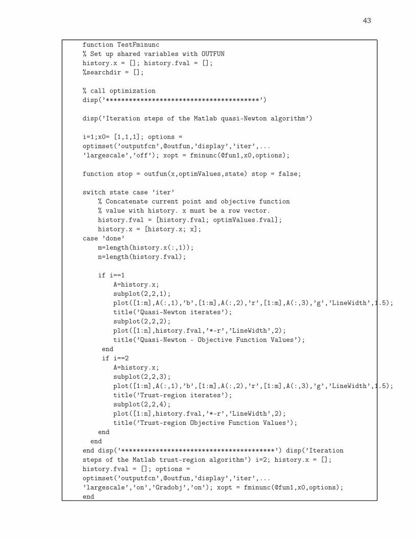
function TestFminunc

% Set up shared variables with OUTFUN

history.x = []; history.fval = [];

%searchdir = [];

% call optimization

disp(’****************************************’)

disp(’Iteration steps of the Matlab quasi-Newton algorithm’)

i=1;x0= [1,1,1]; options =

optimset(’outputfcn’,@outfun,’display’,’iter’,...

’largescale’,’off’); xopt = fminunc(@fun1,x0,options);

function stop = outfun(x,optimValues,state) stop = false;

switch state case ’iter’

% Concatenate current point and objective function

% value with history. x must be a row vector.

history.fval = [history.fval; optimValues.fval];

history.x = [history.x; x];

case ’done’

m=length(history.x(:,1));

n=length(history.fval);

if i==1

A=history.x;

subplot(2,2,1);

plot([1:m],A(:,1),’b’,[1:m],A(:,2),’r’,[1:m],A(:,3),’g’,’LineWidth’,1.5);

title(’Quasi-Newton iterates’);

subplot(2,2,2);

plot([1:n],history.fval,’*-r’,’LineWidth’,2);

title(’Quasi-Newton - Objective Function Values’);

end

if i==2

A=history.x;

subplot(2,2,3);

plot([1:m],A(:,1),’b’,[1:m],A(:,2),’r’,[1:m],A(:,3),’g’,’LineWidth’,1.5);

title(’Trust-region iterates’);

subplot(2,2,4);

plot([1:n],history.fval,’*-r’,’LineWidth’,2);

title(’Trust-region Objective Function Values’);

end

end

end disp(’****************************************’) disp(’Iteration

steps of the Matlab trust-region algorithm’) i=2; history.x = [];

history.fval = []; options =

optimset(’outputfcn’,@outfun,’display’,’iter’,...

’largescale’,’on’,’Gradobj’,’on’); xopt = fminunc(@fun1,x0,options);

end

44

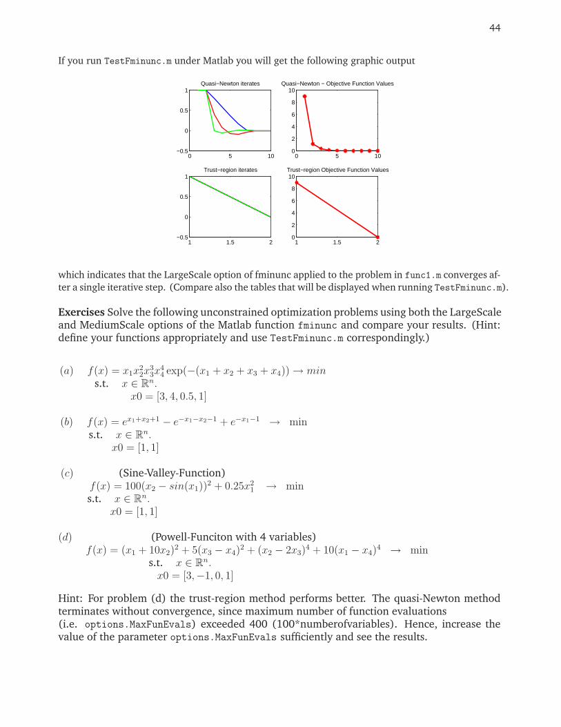
If you run TestFminunc.m under Matlab you will get the following graphic output

0 5 10−0.5

0

0.5

1Quasi−Newton iterates

0 5 100

2

4

6

8

10Quasi−Newton − Objective Function Values

1 1.5 2−0.5

0

0.5

1Trust−region iterates

1 1.5 20

2

4

6

8

10Trust−region Objective Function Values

which indicates that the LargeScale option of fminunc applied to the problem in func1.m converges af-

ter a single iterative step. (Compare also the tables that will be displayed when running TestFminunc.m).

Exercises Solve the following unconstrained optimization problems using both the LargeScaleand MediumScale options of the Matlab function fminunc and compare your results. (Hint:define your functions appropriately and use TestFminunc.m correspondingly.)

(a) f(x) = x1x22x

33x

44 exp(−(x1 + x2 + x3 + x4))→ min

s.t. x ∈ Rn.

x0 = [3, 4, 0.5, 1]

(b) f(x) = ex1+x2+1 − e−x1−x2−1 + e−x1−1 → mins.t. x ∈ R

n.

x0 = [1, 1]

(c) (Sine-Valley-Function)f(x) = 100(x2 − sin(x1))

2 + 0.25x21 → min

s.t. x ∈ Rn.

x0 = [1, 1]

(d) (Powell-Funciton with 4 variables)f(x) = (x1 + 10x2)

2 + 5(x3 − x4)2 + (x2 − 2x3)

4 + 10(x1 − x4)4 → min

s.t. x ∈ Rn.

x0 = [3,−1, 0, 1]

Hint: For problem (d) the trust-region method performs better. The quasi-Newton methodterminates without convergence, since maximum number of function evaluations(i.e. options.MaxFunEvals) exceeded 400 (100*numberofvariables). Hence, increase thevalue of the parameter options.MaxFunEvals sufficiently and see the results.

45

4.7 Derivative free Optimization - direct (simplex) search methods

The Matlab fminsearch.m function uses the Nelder-Mead direct search (also called simplexsearch) algorithm. This method requires only function evaluations, but not derivatives. Assuch the method is useful when

• the derivative of the objective function is expensive to compute;

• exact first derivatives of f are difficult to compute or f has discontinuities;

• the values of f are ’noisy’.

There are many practical optimization problems which exhibit some or all of the the abovedifficult properties. In particular, if the objective function is a result of some experimental(sampled) data, this might usually be the case.

Let f : Rn → R be a function. A simplex S in R

n is a polyhedral set with n + 1 verticesx1, x2, . . . , xn+1 ∈ R

n such that the set xk − xi | k ∈ 1, . . . , n + 1 \ i is linearly indepen-dent in R

n. A simplex S is non-degenerate if none of its three vertices lie on a line or if noneof its four points lie on a hyperplane, etc.

Thus the Nelder-Mead simplex algorithms search the approximate minimum of a function bycomparing the values of the function on the vertices of a simplex. Accordingly, Sk is a simplexat k-th step of the algorithm with ordered vertices xk

1, xk2, . . . , x

kn+1 in such a way that

f(xk1) ≤ f(xk

2) ≤ . . . ≤ f(xkn+1).

Hence, xkn+1 is termed the ’worst’ vertex, xk

n the next ’worst’ vertex, etc., for the minimization,while xk

1 is the ’best’ vertex. Thus a new simplex Sk+1 will be determined by dropping verticeswhich yield larger function values and including new vertices which yield reduced functionvalues, but all the time keeping the number of vertices n + 1 (1 plus problem dimension).This is achieved through reflection, expansion, contraction or shrinking of the simplex Sk. Ineach step it is expected that Sk 6= Sk+1 and the the resulting simplices remain non-degenerate.

Nelder-Mead Algorithm(see Wright et. al. [6, 13] for details)

Step 0: Start with a non-degenerate simplex S0 with vertices x01, x

02, . . . , x

0n+1. Choose the

constantsρ > 0, χ > 1 (χ > ρ), 0 < γ < 1, and 0 < σ < 1

known as reflection, expansion, contraction and shrinkage parameters, respectively.

While (1)

Step 1: Set k ← k + 1 and label the vertices of the simplex Sk so that xk1, x

k2, . . . , x

kn+1

according tof(xk

1) ≤ f(xk2) ≤ . . . ≤ f(xk

n+1).

Step 2: Reflect

46

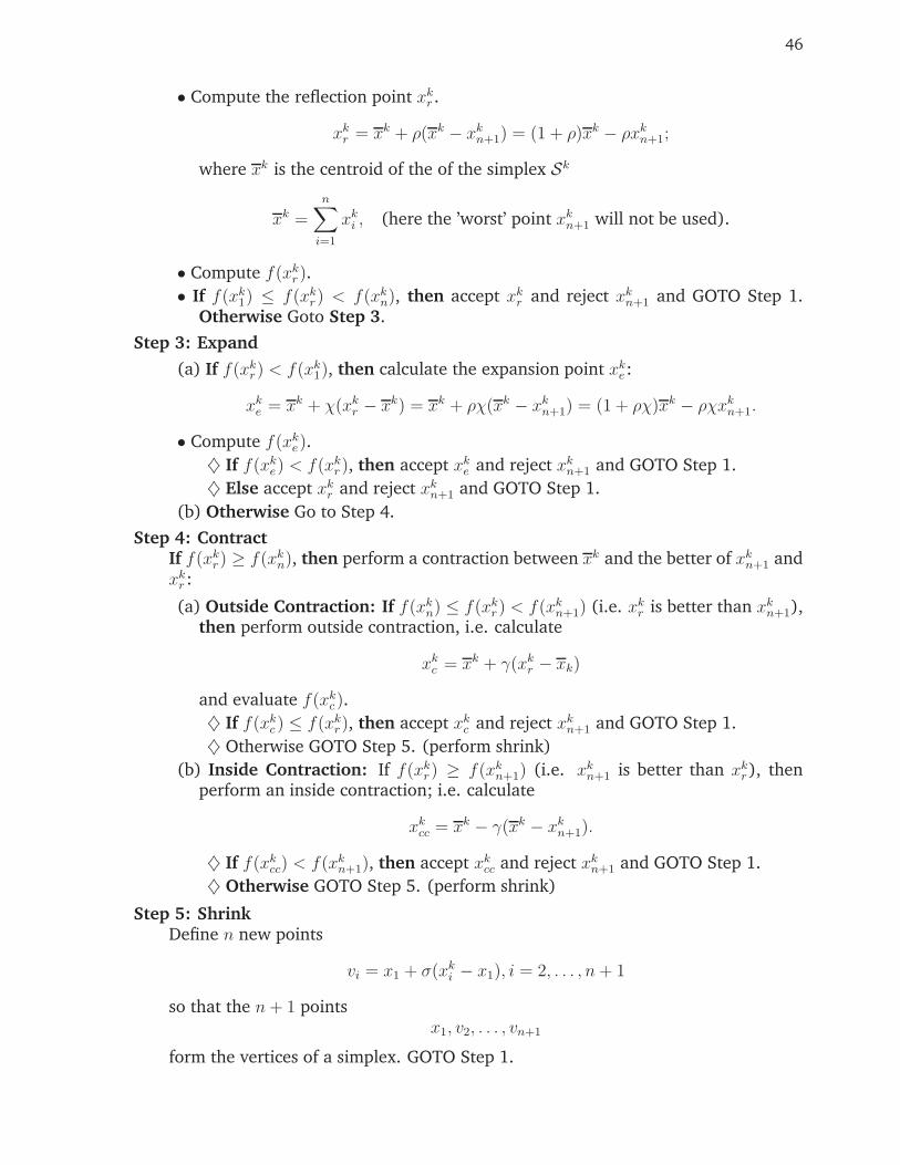
• Compute the reflection point xkr .

xkr = xk + ρ(xk − xk

n+1) = (1 + ρ)xk − ρxkn+1;

where xk is the centroid of the of the simplex Sk

xk =n∑

i=1

xki , (here the ’worst’ point xk

n+1 will not be used).

• Compute f(xkr).

• If f(xk1) ≤ f(xk

r) < f(xkn), then accept xk

r and reject xkn+1 and GOTO Step 1.

Otherwise Goto Step 3.

Step 3: Expand

(a) If f(xkr) < f(xk

1), then calculate the expansion point xke :

xke = xk + χ(xk

r − xk) = xk + ρχ(xk − xkn+1) = (1 + ρχ)xk − ρχxk

n+1.

• Compute f(xke).

♦ If f(xke) < f(xk

r), then accept xke and reject xk

n+1 and GOTO Step 1.

♦ Else accept xkr and reject xk

n+1 and GOTO Step 1.

(b) Otherwise Go to Step 4.

Step 4: ContractIf f(xk

r) ≥ f(xkn), then perform a contraction between xk and the better of xk

n+1 andxk

r :

(a) Outside Contraction: If f(xkn) ≤ f(xk

r) < f(xkn+1) (i.e. xk

r is better than xkn+1),

then perform outside contraction, i.e. calculate

xkc = xk + γ(xk

r − xk)

and evaluate f(xkc ).

♦ If f(xkc ) ≤ f(xk

r), then accept xkc and reject xk

n+1 and GOTO Step 1.

♦ Otherwise GOTO Step 5. (perform shrink)

(b) Inside Contraction: If f(xkr) ≥ f(xk

n+1) (i.e. xkn+1 is better than xk

r), thenperform an inside contraction; i.e. calculate

xkcc = xk − γ(xk − xk

n+1).

♦ If f(xkcc) < f(xk

n+1), then accept xkcc and reject xk

n+1 and GOTO Step 1.

♦ Otherwise GOTO Step 5. (perform shrink)

Step 5: ShrinkDefine n new points

vi = x1 + σ(xki − x1), i = 2, . . . , n + 1

so that the n + 1 pointsx1, v2, . . . , vn+1

form the vertices of a simplex. GOTO Step 1.

47

END

Unfortunately, to date, there is no concrete convergence property that has been proved ofthe original Nelder-Mead algorithm. The algorithm might even converge to a non-stationarypoint of the objective function (see Mickinnon[7] for an example). However, in general, ithas been tested to provide rapid reduction in function values and successful implementationsof the algorithm usually terminate with bounded level sets that contain possible minimumpoints. Recently, there are several attempts to modify the Nelder-Mead algorithm to comeup with convergent variants. Among these: the fortified-descent simplical search method (Tseng [12]) and a multidimensional search algorithm (Torczon [11]) are two of the mostsuccessful ones. See Kelley [5] for a Matlab implementation of the multidimensional searchalgorithm of Torczon.

Bibliography

[1] R. H. Byrd and R. B. Schnabel, Approximate solution of the trust-region problem byminimization over two-dimensional subspaces. Math. Prog. V. 40, pp. 247-263, 1988.

[2] A. Conn, A. I . M. Gould, P. L. Toint, Trust-region methods. SIAM 2000.

[3] D. M. Gay, Computing optimal locally constrained steps. SIAM J. Sci. Stat. Comput. V.2., pp. 186 - 197, 1981.

[4] C. Geiger and C. Kanzow, Numerische Verfahren zur Lösung unrestringierte Opti-mierungsaufgaben. Springer-Verlag, 1999.

[5] C. T. Kelley, Iterative Methods for Optimization. SIAM, 1999.

[6] J. C. Larigas, J. A. Reeds, M. H. Wright and P. E. Wright, Convergence properties of theNelder-Mead simplex method in low dimensions. SIAM J. Optim. V. 9, pp. 112-147.

[7] K. I. M. McKinnon, Convergence of the Nelder-Mead simplex method to a nonstationarypoint. SIAM Journal on Optimization. V. 9, pp. 148 - 158, 1998.

[8] J. A. Nelder and R. Mead, A simplex method for function minimization, Computer Jour-nal, V. 7, pp. 308-313, 1965.

[9] G. A. Schultz, R. B. Schnabel and R. H. Byrd, A family of trust-region-based algorithmsfor uncostrained minimization with strong global convergence properties. SIAM J. Nu-mer. Anal., V. 22, pp. 47- 67, 1985.

[10] D. C. Sorensen, Newton’s method with a model trust region modification. SIAM J. Op-tim., V. 19, pp. 409-426, 1982.

[11] V. Torczon, On the convergence of multidimensional search algorithm. SIAM J. Optim.,V. 1, pp. 123-145.

[12] P. Tseng, Fortified-descent simplical search metho. SIAM J. Optim., Vol. 10, pp. 269-288,1999.

[13] M. H. Wright, Direct search methods: Once scorned, now respectable, in NumericalAnalysis 1995 (ed. D. F. Griffiths and G. A. Watson). Longman, Harlow, pp. 191-208,1996.

[14] W. H. Press, Numerical recipes in C : the art of scientific computing. Cambridge Univ.Press, 2002.

48