solvingpdesinpython –thefenicstutorialvolumei · · 2018-01-22index..... 145. preface...
TRANSCRIPT
Hans Petter Langtangen∗, Anders Logg†
Solving PDEs in Python– The FEniCS Tutorial Volume ISep 18, 2017
Springer
∗Center for Biomedical Computing, Simula Research Laboratory and Department ofInformatics, University of Oslo.
†Email: [email protected]. Department of Mathematical Sciences, ChalmersUniversity of Technology; Center for Biomedical Computing, Simula ResearchLaboratory; and Computational Engineering and Design, Fraunhofer-Chalmers Centre.


Contents
Preface . . . . . . . . . . . . . . . . . . . . . . . . . . . . . . . . . . . . . . . . . . . . . . . . . . . . . . . 1
1 Preliminaries . . . . . . . . . . . . . . . . . . . . . . . . . . . . . . . . . . . . . . . . . . . . . 31.1 The FEniCS Project . . . . . . . . . . . . . . . . . . . . . . . . . . . . . . . . . . . . 31.2 What you will learn . . . . . . . . . . . . . . . . . . . . . . . . . . . . . . . . . . . . 41.3 Working with this tutorial . . . . . . . . . . . . . . . . . . . . . . . . . . . . . . . 41.4 Obtaining the software . . . . . . . . . . . . . . . . . . . . . . . . . . . . . . . . . . 5
1.4.1 Installation using Docker containers . . . . . . . . . . . . . . . . 61.4.2 Installation using Ubuntu packages . . . . . . . . . . . . . . . . . 71.4.3 Testing your installation . . . . . . . . . . . . . . . . . . . . . . . . . . 8
1.5 Obtaining the tutorial examples . . . . . . . . . . . . . . . . . . . . . . . . . . 81.6 Background knowledge . . . . . . . . . . . . . . . . . . . . . . . . . . . . . . . . . . 8
1.6.1 Programming in Python . . . . . . . . . . . . . . . . . . . . . . . . . . . 81.6.2 The finite element method . . . . . . . . . . . . . . . . . . . . . . . . . 9
2 Fundamentals: Solving the Poisson equation . . . . . . . . . . . . . . 112.1 Mathematical problem formulation . . . . . . . . . . . . . . . . . . . . . . . 11
2.1.1 Finite element variational formulation . . . . . . . . . . . . . . . 122.1.2 Abstract finite element variational formulation . . . . . . . 152.1.3 Choosing a test problem . . . . . . . . . . . . . . . . . . . . . . . . . . 16
2.2 FEniCS implementation . . . . . . . . . . . . . . . . . . . . . . . . . . . . . . . . . 172.2.1 The complete program . . . . . . . . . . . . . . . . . . . . . . . . . . . . 172.2.2 Running the program . . . . . . . . . . . . . . . . . . . . . . . . . . . . . 18
2.3 Dissection of the program . . . . . . . . . . . . . . . . . . . . . . . . . . . . . . . 192.3.1 The important first line . . . . . . . . . . . . . . . . . . . . . . . . . . . 192.3.2 Generating simple meshes . . . . . . . . . . . . . . . . . . . . . . . . . 202.3.3 Defining the finite element function space . . . . . . . . . . . 202.3.4 Defining the trial and test functions . . . . . . . . . . . . . . . . 202.3.5 Defining the boundary conditions . . . . . . . . . . . . . . . . . . . 212.3.6 Defining the source term . . . . . . . . . . . . . . . . . . . . . . . . . . 242.3.7 Defining the variational problem . . . . . . . . . . . . . . . . . . . 24
c© 2017, Hans Petter Langtangen, Anders Logg.Released under CC Attribution 4.0 license

vi Contents
2.3.8 Forming and solving the linear system . . . . . . . . . . . . . . 252.3.9 Plotting the solution using the plot command . . . . . . . 252.3.10 Plotting the solution using ParaView . . . . . . . . . . . . . . . 272.3.11 Computing the error . . . . . . . . . . . . . . . . . . . . . . . . . . . . . . 282.3.12 Examining degrees of freedom and vertex values . . . . . . 29
2.4 Deflection of a membrane . . . . . . . . . . . . . . . . . . . . . . . . . . . . . . . . 302.4.1 Scaling the equation . . . . . . . . . . . . . . . . . . . . . . . . . . . . . . 312.4.2 Defining the mesh . . . . . . . . . . . . . . . . . . . . . . . . . . . . . . . . 322.4.3 Defining the load . . . . . . . . . . . . . . . . . . . . . . . . . . . . . . . . . 322.4.4 Defining the variational problem . . . . . . . . . . . . . . . . . . . 332.4.5 Plotting the solution . . . . . . . . . . . . . . . . . . . . . . . . . . . . . . 332.4.6 Making curve plots through the domain . . . . . . . . . . . . . 34
3 A Gallery of finite element solvers . . . . . . . . . . . . . . . . . . . . . . . . 373.1 The heat equation . . . . . . . . . . . . . . . . . . . . . . . . . . . . . . . . . . . . . . 37
3.1.1 PDE problem . . . . . . . . . . . . . . . . . . . . . . . . . . . . . . . . . . . . 373.1.2 Variational formulation . . . . . . . . . . . . . . . . . . . . . . . . . . . 383.1.3 FEniCS implementation . . . . . . . . . . . . . . . . . . . . . . . . . . . 40
3.2 A nonlinear Poisson equation . . . . . . . . . . . . . . . . . . . . . . . . . . . . 463.2.1 PDE problem . . . . . . . . . . . . . . . . . . . . . . . . . . . . . . . . . . . . 463.2.2 Variational formulation . . . . . . . . . . . . . . . . . . . . . . . . . . . 473.2.3 FEniCS implementation . . . . . . . . . . . . . . . . . . . . . . . . . . . 47
3.3 The equations of linear elasticity . . . . . . . . . . . . . . . . . . . . . . . . . 503.3.1 PDE problem . . . . . . . . . . . . . . . . . . . . . . . . . . . . . . . . . . . . 513.3.2 Variational formulation . . . . . . . . . . . . . . . . . . . . . . . . . . . 513.3.3 FEniCS implementation . . . . . . . . . . . . . . . . . . . . . . . . . . . 52
3.4 The Navier–Stokes equations . . . . . . . . . . . . . . . . . . . . . . . . . . . . . 563.4.1 PDE problem . . . . . . . . . . . . . . . . . . . . . . . . . . . . . . . . . . . . 563.4.2 Variational formulation . . . . . . . . . . . . . . . . . . . . . . . . . . . 573.4.3 FEniCS implementation . . . . . . . . . . . . . . . . . . . . . . . . . . . 60
3.5 A system of advection–diffusion–reaction equations . . . . . . . . . 733.5.1 PDE problem . . . . . . . . . . . . . . . . . . . . . . . . . . . . . . . . . . . . 733.5.2 Variational formulation . . . . . . . . . . . . . . . . . . . . . . . . . . . 753.5.3 FEniCS implementation . . . . . . . . . . . . . . . . . . . . . . . . . . . 76
4 Subdomains and boundary conditions . . . . . . . . . . . . . . . . . . . . . 834.1 Combining Dirichlet and Neumann conditions . . . . . . . . . . . . . . 83
4.1.1 PDE problem . . . . . . . . . . . . . . . . . . . . . . . . . . . . . . . . . . . . 834.1.2 Variational formulation . . . . . . . . . . . . . . . . . . . . . . . . . . . 844.1.3 FEniCS implementation . . . . . . . . . . . . . . . . . . . . . . . . . . . 85
4.2 Setting multiple Dirichlet conditions . . . . . . . . . . . . . . . . . . . . . . 864.3 Defining subdomains for different materials . . . . . . . . . . . . . . . . 87
4.3.1 Using expressions to define subdomains . . . . . . . . . . . . . 884.3.2 Using mesh functions to define subdomains . . . . . . . . . . 884.3.3 Using C++ code snippets to define subdomains . . . . . . 91
Contents vii
4.4 Setting multiple Dirichlet, Neumann, and Robin conditions . . 924.4.1 Three types of boundary conditions . . . . . . . . . . . . . . . . . 934.4.2 PDE problem . . . . . . . . . . . . . . . . . . . . . . . . . . . . . . . . . . . . 934.4.3 Variational formulation . . . . . . . . . . . . . . . . . . . . . . . . . . . 944.4.4 FEniCS implementation . . . . . . . . . . . . . . . . . . . . . . . . . . . 954.4.5 Test problem . . . . . . . . . . . . . . . . . . . . . . . . . . . . . . . . . . . . 974.4.6 Debugging boundary conditions . . . . . . . . . . . . . . . . . . . . 98
4.5 Generating meshes with subdomains . . . . . . . . . . . . . . . . . . . . . . 994.5.1 PDE problem . . . . . . . . . . . . . . . . . . . . . . . . . . . . . . . . . . . . 1004.5.2 Variational formulation . . . . . . . . . . . . . . . . . . . . . . . . . . . 1024.5.3 FEniCS implementation . . . . . . . . . . . . . . . . . . . . . . . . . . . 102
5 Extensions: Improving the Poisson solver . . . . . . . . . . . . . . . . . 1095.1 Refactoring the Poisson solver . . . . . . . . . . . . . . . . . . . . . . . . . . . . 109
5.1.1 A more general solver function . . . . . . . . . . . . . . . . . . . . . 1105.1.2 Writing the solver as a Python module . . . . . . . . . . . . . . 1115.1.3 Verification and unit tests . . . . . . . . . . . . . . . . . . . . . . . . . 1115.1.4 Parameterizing the number of space dimensions . . . . . . 114
5.2 Working with linear solvers . . . . . . . . . . . . . . . . . . . . . . . . . . . . . . 1155.2.1 Choosing a linear solver and preconditioner . . . . . . . . . . 1155.2.2 Choosing a linear algebra backend . . . . . . . . . . . . . . . . . . 1155.2.3 Setting solver parameters . . . . . . . . . . . . . . . . . . . . . . . . . . 1165.2.4 An extended solver function . . . . . . . . . . . . . . . . . . . . . . . 1175.2.5 A remark regarding unit tests . . . . . . . . . . . . . . . . . . . . . . 1175.2.6 List of linear solver methods and preconditioners . . . . . 117
5.3 High-level and low-level solver interfaces . . . . . . . . . . . . . . . . . . . 1185.3.1 Linear variational problem and solver objects . . . . . . . . 1185.3.2 Explicit assembly and solve . . . . . . . . . . . . . . . . . . . . . . . . 1195.3.3 Examining matrix and vector values . . . . . . . . . . . . . . . . 122
5.4 Degrees of freedom and function evaluation . . . . . . . . . . . . . . . . 1235.4.1 Examining the degrees of freedom . . . . . . . . . . . . . . . . . . 1235.4.2 Setting the degrees of freedom . . . . . . . . . . . . . . . . . . . . . 1255.4.3 Function evaluation . . . . . . . . . . . . . . . . . . . . . . . . . . . . . . . 126
5.5 Postprocessing computations . . . . . . . . . . . . . . . . . . . . . . . . . . . . . 1275.5.1 Test problem . . . . . . . . . . . . . . . . . . . . . . . . . . . . . . . . . . . . 1275.5.2 Flux computations . . . . . . . . . . . . . . . . . . . . . . . . . . . . . . . 1285.5.3 Computing functionals . . . . . . . . . . . . . . . . . . . . . . . . . . . . 1305.5.4 Computing convergence rates . . . . . . . . . . . . . . . . . . . . . . 1325.5.5 Taking advantage of structured mesh data . . . . . . . . . . . 136
5.6 Taking the next step . . . . . . . . . . . . . . . . . . . . . . . . . . . . . . . . . . . . 141
References . . . . . . . . . . . . . . . . . . . . . . . . . . . . . . . . . . . . . . . . . . . . . . . . . . . . 143
viii Contents
Index . . . . . . . . . . . . . . . . . . . . . . . . . . . . . . . . . . . . . . . . . . . . . . . . . . . . . . . . . 145

Preface
This book gives a concise and gentle introduction to finite element program-ming in Python based on the popular FEniCS software library. FEniCS canbe programmed in both C++ and Python, but this tutorial focuses exclu-sively on Python programming, since this is the simplest and most effectiveapproach for beginners. After having digested the examples in this tutorial,the reader should be able to learn more from the FEniCS documentation, thenumerous demo programs that come with the software, and the comprehen-sive FEniCS book Automated Solution of Differential Equations by the FiniteElement Method [26]. This tutorial is a further development of the openingchapter in [26].
We thank Johan Hake, Kent-Andre Mardal, and Kristian Valen-Sendstadfor many helpful discussions during the preparation of the first version of thistutorial for the FEniCS book [26]. We are particularly thankful to ProfessorDouglas Arnold for very valuable feedback on early versions of the text. Øys-tein Sørensen pointed out numerous typos and contributed with many helpfulcomments. Many errors and typos were also reported by Mauricio Ange-les, Ida Drøsdal, Miroslav Kuchta, Hans Ekkehard Plesser, Marie Rognes,Hans Joachim Scroll, Glenn Terje Lines, Simon Funke, Matthew Moelter,and Magne Nordaas. Ekkehard Ellmann as well as two anonymous reviewersprovided a series of suggestions and improvements. Special thanks go to Ben-jamin Kehlet for all his work with the mshr tool and for quickly implementingour requests for this tutorial.
Comments and corrections can be reported as issues for the Git repositoryof this book1, or via email to [email protected].
Oslo and Smögen, November 2016 Hans Petter Langtangen, Anders Logg
1https://github.com/hplgit/fenics-tutorial/
c© 2017, Hans Petter Langtangen, Anders Logg.Released under CC Attribution 4.0 license


Chapter 1Preliminaries
1.1 The FEniCS Project
The FEniCS Project is a research and software project aimed at creatingmathematical methods and software for automated computational mathe-matical modeling. This means creating easy, intuitive, efficient, and flexiblesoftware for solving partial differential equations (PDEs) using finite elementmethods. FEniCS was initially created in 2003 and is developed in collabo-ration between researchers from a number of universities and research insti-tutes around the world. For more information about FEniCS and the latestupdates of the FEniCS software and this tutorial, visit the FEniCS web pageat https://fenicsproject.org.
FEniCS consists of a number of building blocks (software components)that together form the FEniCS software: DOLFIN [27], FFC [17], FIAT [16],UFL [1], mshr, and a few others. For an overview, see [26]. FEniCS usersrarely need to think about this internal organization of FEniCS, but sinceeven casual users may sometimes encounter the names of various FEniCScomponents, we briefly list the components and their main roles in FEniCS.DOLFIN is the computational high-performance C++ backend of FEniCS.DOLFIN implements data structures such as meshes, function spaces andfunctions, compute-intensive algorithms such as finite element assembly andmesh refinement, and interfaces to linear algebra solvers and data structuressuch as PETSc. DOLFIN also implements the FEniCS problem-solving en-vironment in both C++ and Python. FFC is the code generation engine ofFEniCS (the form compiler), responsible for generating efficient C++ codefrom high-level mathematical abstractions. FIAT is the finite element back-end of FEniCS, responsible for generating finite element basis functions, UFLimplements the abstract mathematical language by which users may expressvariational problems, and mshr provides FEniCS with mesh generation ca-pabilities.
c© 2017, Hans Petter Langtangen, Anders Logg.Released under CC Attribution 4.0 license

4 1 Preliminaries
1.2 What you will learn
The goal of this tutorial is to demonstrate how to apply the finite element tosolve PDEs in FEniCS. Through a series of examples, we demonstrate howto:
• solve linear PDEs (such as the Poisson equation),• solve time-dependent PDEs (such as the heat equation),• solve nonlinear PDEs,• solve systems of time-dependent nonlinear PDEs.
Important topics involve how to set boundary conditions of various types(Dirichlet, Neumann, Robin), how to create meshes, how to define variablecoefficients, how to interact with linear and nonlinear solvers, and how topostprocess and visualize solutions.
We will also discuss how to best structure the Python code for a PDEsolver, how to debug programs, and how to take advantage of testing frame-works.
1.3 Working with this tutorial
The mathematics of the illustrations is kept simple to better focus on FEniCSfunctionality and syntax. This means that we mostly use the Poisson equationand the time-dependent diffusion equation as model problems, often withinput data adjusted such that we get a very simple solution that can beexactly reproduced by any standard finite element method over a uniform,structured mesh. This latter property greatly simplifies the verification of theimplementations. Occasionally we insert a physically more relevant exampleto remind the reader that the step from solving a simple model problem to achallenging real-world problem is often quite short and easy with FEniCS.
Using FEniCS to solve PDEs may seem to require a thorough understand-ing of the abstract mathematical framework of the finite element methodas well as expertise in Python programming. Nevertheless, it turns out thatmany users are able to pick up the fundamentals of finite elements and Pythonprogramming as they go along with this tutorial. Simply keep on reading andtry out the examples. You will be amazed at how easy it is to solve PDEswith FEniCS!

1.4 Obtaining the software 5
1.4 Obtaining the software
Working with this tutorial obviously requires access to the FEniCS software.FEniCS is a complex software library, both in itself and due to its many de-pendencies to state-of-the-art open-source scientific software libraries. Man-ually building FEniCS and all its dependencies from source can thus be adaunting task. Even for an expert who knows exactly how to configure andbuild each component, a full build can literally take hours! In addition to thecomplexity of the software itself, there is an additional layer of complexity inhow many different kinds of operating systems (Linux, Mac, Windows) maybe running on a user’s laptop or compute server, with different requirementsfor how to configure and build software.
For this reason, the FEniCS Project provides prebuilt packages to makethe installation easy, fast, and foolproof.
FEniCS download and installationIn this tutorial, we highlight two main options for installing the FEniCSsoftware: Docker containers and Ubuntu packages. While the Dockercontainers work on all operating systems, the Ubuntu packages onlywork on Ubuntu-based systems. Note that the built-in FEniCS plottingdoes currently not work from Docker, although rudimentary plotting issupported via the Docker Jupyter notebook option.
FEniCS may also be installed using other methods, including Condapackages and building from source. For more installation options andthe latest information on the simplest and best options for installingFEniCS, check out the official FEniCS installation instructions. Thesecan be found at https://fenicsproject.org/download.
FEniCS version: 2016.2FEniCS versions are labeled 2016.1, 2016.2, 2017.1 and so on, where themajor number indicates the year of release and the minor number is acounter starting at 1. The number of releases per year varies but typi-cally one can expect 2–3 releases per year. This tutorial was preparedfor and tested with FEniCS version 2016.2.
6 1 Preliminaries
1.4.1 Installation using Docker containers
A modern solution to the challenge of software installation on diverse soft-ware platforms is to use so-called containers. The FEniCS Project pro-vides custom-made containers that are controlled, consistent, and high-performance software environments for FEniCS programming. FEniCS con-tainers work equally well1 on all operating systems, including Linux, Mac,and Windows.
To use FEniCS containers, you must first install the Docker platform.Docker installation is simple and instructions are available on the Dockerweb page2. Once you have installed Docker, just copy the following line intoa terminal window:
Terminal
Terminal> curl -s https://get.fenicsproject.org | bash
The command above will install the program fenicsproject on your sys-tem. This program lets you easily create FEniCS sessions (containers) onyour system:
Terminal
Terminal> fenicsproject run
This command has several useful options, such as easily switching betweenthe latest release of FEniCS, the latest development version and many more.To learn more, type fenicsproject help. FEniCS can also be used directlywith Docker, but this typically requires typing a relatively complex Dockercommand, for example:
Terminal
docker run --rm -ti -v ‘pwd‘:/home/fenics/shared -w/home/fenics/shared quay.io/fenicsproject/stable:current ’/bin/bash -l-c "export TERM=xterm; bash -i"’
Sharing files with FEniCS containers
When you run a FEniCS session using fenicsproject run, it will au-tomatically share your current working directory (the directory from
1Running Docker containers on Mac and Windows involves a small performanceoverhead compared to running Docker containers on Linux. However, this performancepenalty is typically small and is often compensated for by using the highly tuned andoptimized version of FEniCS that comes with the official FEniCS containers, comparedto building FEniCS and its dependencies from source on Mac or Windows.
2https://www.docker.com

1.4 Obtaining the software 7
which you run the fenicsproject command) with the FEniCS ses-sion. When the FEniCS session starts, it will automatically enter intoa directory named shared which will be identical with your currentworking directory on your host system. This means that you can eas-ily edit files and write data inside the FEniCS session, and the fileswill be directly accessible on your host system. It is recommended thatyou edit your programs using your favorite editor (such as Emacs orVim) on your host system and use the FEniCS session only to run yourprogram(s).
1.4.2 Installation using Ubuntu packages
For users of Ubuntu GNU/Linux, FEniCS can also be installed easily via thestandard Ubuntu package manager apt-get. Just copy the following linesinto a terminal window:
Terminal
Terminal> sudo add-apt-repository ppa:fenics-packages/fenicsTerminal> sudo apt-get updateTerminal> sudo apt-get install fenicsTerminal> sudo apt-get dist-upgrade
This will add the FEniCS package archive (PPA) to your Ubuntu com-puter’s list of software sources and then install FEniCS. It will will alsoautomatically install packages for dependencies of FEniCS.
Watch out for old packages!
In addition to being available from the FEniCS PPA, the FEniCS soft-ware is also part of the official Ubuntu repositories. However, dependingon which release of Ubuntu you are running, and when this release wascreated in relation to the latest FEniCS release, the official Ubunturepositories might contain an outdated version of FEniCS. For this rea-son, it is better to install from the FEniCS PPA.
8 1 Preliminaries
1.4.3 Testing your installation
Once you have installed FEniCS, you should make a quick test to see thatyour installation works properly. To do this, type the following command ina FEniCS-enabled3 terminal:
Terminal
Terminal> python -c ’import fenics’
If all goes well, you should be able to run this command without any errormessage (or any other output).
1.5 Obtaining the tutorial examples
In this tutorial, you will learn finite element and FEniCS programmingthrough a number of example programs that demonstrate both how to solveparticular PDEs using the finite element method, how to program solvers inFEniCS, and how to create well-designed Python code that can later be ex-tended to solve more complex problems. All example programs are availablefrom the web page of this book at https://fenicsproject.org/tutorial.The programs as well as the source code for this text can also be accesseddirectly from the Git repository4 for this book.
1.6 Background knowledge
1.6.1 Programming in Python
While you can likely pick up basic Python programming by working throughthe examples in this tutorial, you may want to study additional materialon the Python language. A natural starting point for beginners is the classicPython Tutorial [11], or a tutorial geared towards scientific computing [22]. Inthe latter, you will also find pointers to other tutorials for scientific computingin Python. Among ordinary books we recommend the general introductionDive into Python [28] as well as texts that focus on scientific computing withPython [15,18–21].
3For users of FEniCS containers, this means first running the commandfenicsproject run.
4https://github.com/hplgit/fenics-tutorial/

1.6 Background knowledge 9
Python versions
Python comes in two versions, 2 and 3, and these are not compatible.FEniCS works with both versions of Python. All the programs in thistutorial are also developed such that they can be run under both Python2 and 3. Python programs that need to print must then start with
from __future__ import print_function
to enable the print function from Python 3 in Python 2. All use ofprint in the programs in this tutorial consists of function calls, likeprint(’a:’, a). Almost all other constructions are of a form thatlooks the same in Python 2 and 3.
1.6.2 The finite element method
Many good books have been written on the finite element method. The bookstypically fall in either of two categories: the abstract mathematical versionof the method or the engineering “structural analysis” formulation. FEniCSbuilds heavily on concepts from the abstract mathematical exposition. Thefirst author has a book5 [24] in development that explains all details of thefinite element method in an intuitive way, using the abstract mathematicalformulations that FEniCS employs.
The finite element text by Larson and Bengzon [25] is our recommendedintroduction to the finite element method, with a mathematical notationthat goes well with FEniCS. An easy-to-read book, which also provides agood general background for using FEniCS, is Gockenbach [12]. The bookby Donea and Huerta [8] has a similar style, but aims at readers with aninterest in fluid flow problems. Hughes [14] is also recommended, especiallyfor readers interested in solid mechanics and heat transfer applications.
Readers with a background in the engineering “structural analysis” versionof the finite element method may find Bickford [3] an attractive bridge over tothe abstract mathematical formulation that FEniCS builds upon. Those whohave a weak background in differential equations in general should consulta more fundamental book, and Eriksson et al [9] is a very good choice. Onthe other hand, FEniCS users with a strong background in mathematics willappreciate the texts by Brenner and Scott [5], Braess [4], Ern and Guermond[10], Quarteroni and Valli [29], or Ciarlet [7].
5http://hplgit.github.io/fem-book/doc/web/index.html

Chapter 2Fundamentals: Solving the Poissonequation
The goal of this chapter is to show how the Poisson equation, the most basic ofall PDEs, can be quickly solved with a few lines of FEniCS code. We introducethe most fundamental FEniCS objects such as Mesh, Function, FunctionSpace,TrialFunction, and TestFunction, and learn how to write a basic PDE solver,including how to formulate the mathematical variational problem, apply boundaryconditions, call the FEniCS solver, and plot the solution.
2.1 Mathematical problem formulation
Many books on programming languages start with a “Hello, World!” program.Readers are curious to know how fundamental tasks are expressed in thelanguage, and printing a text to the screen can be such a task. In the worldof finite element methods for PDEs, the most fundamental task must be tosolve the Poisson equation. Our counterpart to the classical “Hello, World!”program therefore solves the following boundary-value problem:
−∇2u(x) = f(x), x in Ω, (2.1)u(x) = uD(x), x on ∂Ω . (2.2)
Here, u = u(x) is the unknown function, f = f(x) is a prescribed function,∇2 is the Laplace operator (often written as ∆), Ω is the spatial domain,and ∂Ω is the boundary of Ω. The Poisson problem, including both thePDE −∇2u = f and the boundary condition u = uD on ∂Ω, is an exampleof a boundary-value problem, which must be precisely stated before it makessense to start solving it with FEniCS.
In two space dimensions with coordinates x and y, we can write out thePoisson equation as
c© 2017, Hans Petter Langtangen, Anders Logg.Released under CC Attribution 4.0 license

12 2 Fundamentals: Solving the Poisson equation
− ∂2u
∂x2 −∂2u
∂y2 = f(x,y) . (2.3)
The unknown u is now a function of two variables, u = u(x,y), defined overa two-dimensional domain Ω.
The Poisson equation arises in numerous physical contexts, including heatconduction, electrostatics, diffusion of substances, twisting of elastic rods, in-viscid fluid flow, and water waves. Moreover, the equation appears in numer-ical splitting strategies for more complicated systems of PDEs, in particularthe Navier–Stokes equations.
Solving a boundary-value problem such as the Poisson equation in FEniCSconsists of the following steps:
1. Identify the computational domain (Ω), the PDE, its boundary conditions,and source terms (f).
2. Reformulate the PDE as a finite element variational problem.3. Write a Python program which defines the computational domain, the
variational problem, the boundary conditions, and source terms, using thecorresponding FEniCS abstractions.
4. Call FEniCS to solve the boundary-value problem and, optionally, extendthe program to compute derived quantities such as fluxes and averages,and visualize the results.
We shall now go through steps 2–4 in detail. The key feature of FEniCS isthat steps 3 and 4 result in fairly short code, while a similar program in mostother software frameworks for PDEs require much more code and technicallydifficult programming.
What makes FEniCS attractive?Although many software frameworks have a really elegant “Hello,World!” example for the Poisson equation, FEniCS is to our knowl-edge the only framework where the code stays compact and nice, veryclose to the mathematical formulation, even when the mathematicaland algorithmic complexity increases and when moving from a laptopto a high-performance compute server (cluster).
2.1.1 Finite element variational formulation
FEniCS is based on the finite element method, which is a general and efficientmathematical machinery for the numerical solution of PDEs. The startingpoint for the finite element methods is a PDE expressed in variational form.Readers who are not familiar with variational problems will get a very briefintroduction to the topic in this tutorial, but reading a proper book on the

2.1 Mathematical problem formulation 13
finite element method in addition is encouraged. Section 1.6.2 contains a listof recommended books. Experience shows that you can work with FEniCS asa tool to solve PDEs even without thorough knowledge of the finite elementmethod, as long as you get somebody to help you with formulating the PDEas a variational problem.
The basic recipe for turning a PDE into a variational problem is to multiplythe PDE by a function v, integrate the resulting equation over the domain Ω,and perform integration by parts of terms with second-order derivatives. Thefunction v which multiplies the PDE is called a test function. The unknownfunction u to be approximated is referred to as a trial function. The termstrial and test functions are used in FEniCS programs too. The trial andtest functions belong to certain so-called function spaces that specify theproperties of the functions.
In the present case, we first multiply the Poisson equation by the testfunction v and integrate over Ω:
−∫Ω
(∇2u)vdx=∫Ωfvdx. (2.4)
We here let dx denote the differential element for integration over the domainΩ. We will later let ds denote the differential element for integration overthe boundary of Ω.
A common rule when we derive variational formulations is that we try tokeep the order of the derivatives of u and v as small as possible. Here, wehave a second-order spatial derivative of u, which can be transformed to afirst-derivative of u and v by applying the technique of integration by parts1.The formula reads
−∫Ω
(∇2u)vdx=∫Ω∇u ·∇vdx−
∫∂Ω
∂u
∂nvds, (2.5)
where ∂u∂n =∇u ·n is the derivative of u in the outward normal direction n
on the boundary.Another feature of variational formulations is that the test function v is
required to vanish on the parts of the boundary where the solution u is known(the book [24] explains in detail why this requirement is necessary). In thepresent problem, this means that v = 0 on the whole boundary ∂Ω. Thesecond term on the right-hand side of (2.5) therefore vanishes. From (2.4)and (2.5) it follows that ∫
Ω∇u ·∇vdx=
∫Ωfvdx. (2.6)
If we require that this equation holds for all test functions v in some suit-able space V , the so-called test space, we obtain a well-defined mathematicalproblem that uniquely determines the solution u which lies in some (possi-
1https://en.wikipedia.org/wiki/Integration_by_parts

14 2 Fundamentals: Solving the Poisson equation
bly different) function space V , the so-called trial space. We refer to (2.6) asthe weak form or variational form of the original boundary-value problem(2.1)–(2.2).
The proper statement of our variational problem now goes as follows: findu ∈ V such that ∫
Ω∇u ·∇vdx=
∫Ωfvdx ∀v ∈ V . (2.7)
The trial and test spaces V and V are in the present problem defined as
V = v ∈H1(Ω) : v = uD on ∂Ω,V = v ∈H1(Ω) : v = 0 on ∂Ω .
In short, H1(Ω) is the mathematically well-known Sobolev space containingfunctions v such that v2 and |∇v|2 have finite integrals over Ω (essentiallymeaning that the functions are continuous). The solution of the underlyingPDE must lie in a function space where the derivatives are also continuous,but the Sobolev space H1(Ω) allows functions with discontinuous derivatives.This weaker continuity requirement of u in the variational statement (2.7), asa result of the integration by parts, has great practical consequences when itcomes to constructing finite element function spaces. In particular, it allowsthe use of piecewise polynomial function spaces; i.e., function spaces con-structed by stitching together polynomial functions on simple domains suchas intervals, triangles, or tetrahedrons.
The variational problem (2.7) is a continuous problem: it defines the solu-tion u in the infinite-dimensional function space V . The finite element methodfor the Poisson equation finds an approximate solution of the variational prob-lem (2.7) by replacing the infinite-dimensional function spaces V and V bydiscrete (finite-dimensional) trial and test spaces Vh ⊂ V and Vh ⊂ V . Thediscrete variational problem reads: find uh ∈ Vh ⊂ V such that∫
Ω∇uh ·∇vdx=
∫Ωfvdx ∀v ∈ Vh ⊂ V . (2.8)
This variational problem, together with a suitable definition of the func-tion spaces Vh and Vh, uniquely define our approximate numerical solutionof Poisson’s equation (2.1). Note that the boundary conditions are encodedas part of the trial and test spaces. The mathematical framework may seemcomplicated at first glance, but the good news is that the finite element vari-ational problem (2.8) looks the same as the continuous variational problem(2.7), and FEniCS can automatically solve variational problems like (2.8)!
2.1 Mathematical problem formulation 15
What we mean by the notation u and V
The mathematics literature on variational problems writes uh for thesolution of the discrete problem and u for the solution of the continu-ous problem. To obtain (almost) a one-to-one relationship between themathematical formulation of a problem and the corresponding FEniCSprogram, we shall drop the subscript h and use u for the solution of thediscrete problem. We will use ue for the exact solution of the continuousproblem, if we need to explicitly distinguish between the two. Similarly,we will let V denote the discrete finite element function space in whichwe seek our solution.
2.1.2 Abstract finite element variational formulation
It turns out to be convenient to introduce the following canonical notationfor variational problems: find u ∈ V such that
a(u,v) = L(v) ∀v ∈ V . (2.9)
For the Poisson equation, we have:
a(u,v) =∫Ω∇u ·∇vdx, (2.10)
L(v) =∫Ωfvdx. (2.11)
From the mathematics literature, a(u,v) is known as a bilinear form andL(v) as a linear form. We shall, in every linear problem we solve, identify theterms with the unknown u and collect them in a(u,v), and similarly collectall terms with only known functions in L(v). The formulas for a and L canthen be expressed directly in our FEniCS programs.
To solve a linear PDE in FEniCS, such as the Poisson equation, a userthus needs to perform only two steps:
• Choose the finite element spaces V and V by specifying the domain (themesh) and the type of function space (polynomial degree and type).
• Express the PDE as a (discrete) variational problem: find u ∈ V such thata(u,v) = L(v) for all v ∈ V .
16 2 Fundamentals: Solving the Poisson equation
2.1.3 Choosing a test problem
The Poisson problem (2.1)–(2.2) has so far featured a general domain Ω andgeneral functions uD for the boundary conditions and f for the right-handside. For our first implementation we will need to make specific choices forΩ, uD , and f . It will be wise to construct a problem with a known analyticalsolution so that we can easily check that the computed solution is correct.Solutions that are lower-order polynomials are primary candidates. Standardfinite element function spaces of degree r will exactly reproduce polynomialsof degree r. And piecewise linear elements (r = 1) are able to exactly repro-duce a quadratic polynomial on a uniformly partitioned mesh. This importantresult can be used to verify our implementation. We just manufacture somequadratic function in 2D as the exact solution, say
ue(x,y) = 1 +x2 + 2y2 . (2.12)
By inserting (2.12) into the Poisson equation (2.1), we find that ue(x,y) is asolution if
f(x,y) =−6, uD(x,y) = ue(x,y) = 1 +x2 + 2y2,
regardless of the shape of the domain as long as ue is prescribed along theboundary. We choose here, for simplicity, the domain to be the unit square,
Ω = [0,1]× [0,1] .
This simple but very powerful method for constructing test problems is calledthe method of manufactured solutions: pick a simple expression for the exactsolution, plug it into the equation to obtain the right-hand side (source termf), then solve the equation with this right-hand side and using the exactsolution as a boundary condition, and try to reproduce the exact solution.
Tip: Try to verify your code with exact numerical solutions!
A common approach to testing the implementation of a numericalmethod is to compare the numerical solution with an exact analyti-cal solution of the test problem and conclude that the program works ifthe error is “small enough”. Unfortunately, it is impossible to tell if anerror of size 10−5 on a 20×20 mesh of linear elements is the expected(in)accuracy of the numerical approximation or if the error also containsthe effect of a bug in the code. All we usually know about the numericalerror is its asymptotic properties, for instance that it is proportional toh2 if h is the size of a cell in the mesh. Then we compare the erroron meshes with different h-values to see if the asymptotic behavior iscorrect. This is a very powerful verification technique and is explained

2.2 FEniCS implementation 17
in detail in Section 5.5.4. However, if we have a test problem for whichwe know that there should be no approximation errors, we know thatthe analytical solution of the PDE problem should be reproduced tomachine precision by the program. That is why we emphasize this kindof test problems throughout this tutorial. Typically, elements of degreer can reproduce polynomials of degree r exactly, so this is the start-ing point for constructing a solution without numerical approximationerrors.
2.2 FEniCS implementation
2.2.1 The complete program
A FEniCS program for solving our test problem for the Poisson equation in2D with the given choices of Ω, uD , and f may look as follows:
from fenics import *
# Create mesh and define function spacemesh = UnitSquareMesh(8, 8)V = FunctionSpace(mesh, ’P’, 1)
# Define boundary conditionu_D = Expression(’1 + x[0]*x[0] + 2*x[1]*x[1]’, degree=2)
def boundary(x, on_boundary):return on_boundary
bc = DirichletBC(V, u_D, boundary)
# Define variational problemu = TrialFunction(V)v = TestFunction(V)f = Constant(-6.0)a = dot(grad(u), grad(v))*dxL = f*v*dx
# Compute solutionu = Function(V)solve(a == L, u, bc)
# Plot solution and meshplot(u)plot(mesh)
# Save solution to file in VTK formatvtkfile = File(’poisson/solution.pvd’)vtkfile << u

18 2 Fundamentals: Solving the Poisson equation
# Compute error in L2 normerror_L2 = errornorm(u_D, u, ’L2’)
# Compute maximum error at verticesvertex_values_u_D = u_D.compute_vertex_values(mesh)vertex_values_u = u.compute_vertex_values(mesh)import numpy as nperror_max = np.max(np.abs(vertex_values_u_D - vertex_values_u))
# Print errorsprint(’error_L2 =’, error_L2)print(’error_max =’, error_max)
# Hold plotinteractive()
This example program can be found in the file ft01_poisson.py.
2.2.2 Running the program
The FEniCS program must be available in a plain text file, written with atext editor such as Atom, Sublime Text, Emacs, Vim, or similar. There areseveral ways to run a Python program like ft01_poisson.py:
• Use a terminal window.• Use an integrated development environment (IDE), e.g., Spyder.• Use a Jupyter notebook.
Terminal window. Open a terminal window, move to the directory con-taining the program and type the following command:
Terminal
Terminal> python ft01_poisson.py
Note that this command must be run in a FEniCS-enabled terminal. Forusers of the FEniCS Docker containers, this means that you must type thiscommand after you have started a FEniCS session using fenicsproject runor fenicsproject start.
When running the above command, FEniCS will run the program to com-pute the approximate solution u. The approximate solution u will be com-pared to the exact solution ue = uD and the error in the L2 and maximumnorms will be printed. Since we know that our approximate solution shouldreproduce the exact solution to within machine precision, this error should besmall, something on the order of 10−15. If plotting is enabled in your FEniCSinstallation, then a window with a simple plot of the solution will appear asin Figure 2.1.
2.3 Dissection of the program 19
Spyder. Many prefer to work in an integrated development environmentthat provides an editor for programming, a window for executing code, awindow for inspecting objects, etc. Just open the file ft01_poisson.py andpress the play button to run it. We refer to the Spyder tutorial to learn moreabout working in the Spyder environment. Spyder is highly recommended ifyou are used to working in the graphical MATLAB environment.
Jupyter notebooks. Notebooks make it possible to mix text and executablecode in the same document, but you can also just use it to run programs in aweb browser. Run the command jupyter notebook from a terminal window,find the New pulldown menu in the upper right corner of the GUI, choosea new notebook in Python 2 or 3, write %load ft01_poisson.py in theblank cell of this notebook, then press Shift+Enter to execute the cell. Thefile ft01_poisson.py will then be loaded into the notebook. Re-execute thecell (Shift+Enter) to run the program. You may divide the entire programinto several cells to examine intermediate results: place the cursor whereyou want to split the cell and choose Edit - Split Cell. For users of theFEniCS Docker images, run the fenicsproject notebook command andfollow the instructions. To enable plotting, make sure to run the command%matplotlib inline inside the notebook.
2.3 Dissection of the program
We shall now dissect our FEniCS program in detail. The listed FEniCS pro-gram defines a finite element mesh, a finite element function space V on thismesh, boundary conditions for u (the function uD), and the bilinear and lin-ear forms a(u,v) and L(v). Thereafter, the solution u is computed. At theend of the program, we compare the numerical and the exact solutions. Wealso plot the solution using the plot command and save the solution to a filefor external postprocessing.
2.3.1 The important first line
The first line in the program,
from fenics import *
imports the key classes UnitSquareMesh, FunctionSpace, Function, and soforth, from the FEniCS library. All FEniCS programs for solving PDEs bythe finite element method normally start with this line.
20 2 Fundamentals: Solving the Poisson equation
2.3.2 Generating simple meshes
The statement
mesh = UnitSquareMesh(8, 8)
defines a uniform finite element mesh over the unit square [0,1]× [0,1]. Themesh consists of cells, which in 2D are triangles with straight sides. Theparameters 8 and 8 specify that the square should be divided into 8× 8rectangles, each divided into a pair of triangles. The total number of triangles(cells) thus becomes 128. The total number of vertices in the mesh is 9 ·9 = 81.In later chapters, you will learn how to generate more complex meshes.
2.3.3 Defining the finite element function space
Once the mesh has been created, we can create a finite element function spaceV:
V = FunctionSpace(mesh, ’P’, 1)
The second argument ’P’ specifies the type of element. The type of ele-ment here is P, implying the standard Lagrange family of elements. You mayalso use ’Lagrange’ to specify this type of element. FEniCS supports allsimplex element families and the notation defined in the Periodic Table ofthe Finite Elements2 [2].
The third argument 1 specifies the degree of the finite element. In this case,the standard P1 linear Lagrange element, which is a triangle with nodes atthe three vertices. Some finite element practitioners refer to this elementas the “linear triangle”. The computed solution u will be continuous acrosselements and linearly varying in x and y inside each element. Higher-degreepolynomial approximations over each cell are trivially obtained by increasingthe third parameter to FunctionSpace, which will then generate functionspaces of type P2, P3, and so forth. Changing the second parameter to ’DP’creates a function space for discontinuous Galerkin methods.
2.3.4 Defining the trial and test functions
In mathematics, we distinguish between the trial and test spaces V and V .The only difference in the present problem is the boundary conditions. InFEniCS we do not specify the boundary conditions as part of the function
2https://www.femtable.org
2.3 Dissection of the program 21
space, so it is sufficient to work with one common space V for both the trialand test functions in the program:
u = TrialFunction(V)v = TestFunction(V)
2.3.5 Defining the boundary conditions
The next step is to specify the boundary condition: u = uD on ∂Ω. This isdone by
bc = DirichletBC(V, u_D, boundary)
where u_D is an expression defining the solution values on the boundary,and boundary is a function (or object) defining which points belong to theboundary.
Boundary conditions of the type u= uD are known as Dirichlet conditions.For the present finite element method for the Poisson problem, they are alsocalled essential boundary conditions, as they need to be imposed explicitly aspart of the trial space (in contrast to being defined implicitly as part of thevariational formulation). Naturally, the FEniCS class used to define Dirichletboundary conditions is named DirichletBC.
The variable u_D refers to an Expression object, which is used to representa mathematical function. The typical construction is
u_D = Expression(formula, degree=1)
where formula is a string containing a mathematical expression. The for-mula must be written with C++ syntax and is automatically turned into anefficient, compiled C++ function.
Expressions and accuracy
When defining an Expression, the second argument degree is a pa-rameter that specifies how the expression should be treated in compu-tations. On each local element, FEniCS will interpolate the expressioninto a finite element space of the specified degree. To obtain optimal(order of) accuracy in computations, it is usually a good choice to usethe same degree as for the space V that is used for the trial and testfunctions. However, if an Expression is used to represent an exact so-lution which is used to evaluate the accuracy of a computed solution,a higher degree must be used for the expression (one or two degreeshigher).
22 2 Fundamentals: Solving the Poisson equation
The expression may depend on the variables x[0] and x[1] correspond-ing to the x and y coordinates. In 3D, the expression may also depend onthe variable x[2] corresponding to the z coordinate. With our choice ofuD(x,y) = 1+x2 +2y2, the formula string can be written as 1 + x[0]*x[0]+ 2*x[1]*x[1]:
u_D = Expression(’1 + x[0]*x[0] + 2*x[1]*x[1]’, degree=2)
We set the degree to 2 so that u_D may represent the exact quadraticsolution to our test problem.
String expressions must have valid C++ syntax!
The string argument to an Expression object must obey C++ syntax.Most Python syntax for mathematical expressions is also valid C++syntax, but power expressions make an exception: p**a must be writ-ten as pow(p, a) in C++ (this is also an alternative Python syntax).The following mathematical functions can be used directly in C++ ex-pressions when defining Expression objects: cos, sin, tan, acos, asin,atan, atan2, cosh, sinh, tanh, exp, frexp, ldexp, log, log10, modf,pow, sqrt, ceil, fabs, floor, and fmod. Moreover, the number π isavailable as the symbol pi. All the listed functions are taken from thecmath C++ header file, and one may hence consult the documentationof cmath for more information on the various functions.
If/else tests are possible using the C syntax for inline branching. Thefunction
f(x,y) =x2, x,y ≥ 0,2, otherwise,
is implemented as
f = Expression(’x[0]>=0 && x[1]>=0 ? pow(x[0], 2) : 2’, degree=2)
Parameters in expression strings are allowed, but must be initial-ized via keyword arguments when creating the Expression object. Forexample, the function f(x) = e−κπ
2t sin(πkx) can be coded as
f = Expression(’exp(-kappa*pow(pi, 2)*t)*sin(pi*k*x[0])’, degree=2,kappa=1.0, t=0, k=4)
At any time, parameters can be updated:
f.t += dtf.k = 10
The function boundary specifies which points that belong to the part ofthe boundary where the boundary condition should be applied:
2.3 Dissection of the program 23
def boundary(x, on_boundary):return on_boundary
A function like boundary for marking the boundary must return a booleanvalue: True if the given point x lies on the Dirichlet boundary and Falseotherwise. The argument on_boundary is True if x is on the physical bound-ary of the mesh, so in the present case, where we are supposed to returnTrue for all points on the boundary, we can just return the supplied value ofon_boundary. The boundary function will be called for every discrete pointin the mesh, which means that we may define boundaries where u is alsoknown inside the domain, if desired.
One way to think about the specification of boundaries in FEniCS is thatFEniCS will ask you (or rather the function boundary which you have imple-mented) whether or not a specific point x is part of the boundary. FEniCSalready knows whether the point belongs to the actual boundary (the math-ematical boundary of the domain) and kindly shares this information withyou in the variable on_boundary. You may choose to use this information (aswe do here), or ignore it completely.
The argument on_boundary may also be omitted, but in that case we needto test on the value of the coordinates in x:
def boundary(x):return x[0] == 0 or x[1] == 0 or x[0] == 1 or x[1] == 1
Comparing floating-point values using an exact match test with == is not goodprogramming practice, because small round-off errors in the computations ofthe x values could make a test x[0] == 1 become false even though x lies onthe boundary. A better test is to check for equality with a tolerance, eitherexplicitly
tol = 1E-14def boundary(x):
return abs(x[0]) < tol or abs(x[1]) < tol \or abs(x[0] - 1) < tol or abs(x[1] - 1) < tol
or using the near command in FEniCS:
def boundary(x):return near(x[0], 0, tol) or near(x[1], 0, tol) \
or near(x[0], 1, tol) or near(x[1], 1, tol)
Never use == for comparing real numbers!
A comparison like x[0] == 1 should never be used if x[0] is a realnumber, because rounding errors in x[0] may make the test fail evenwhen it is mathematically correct. Consider the following calculationsin Python:
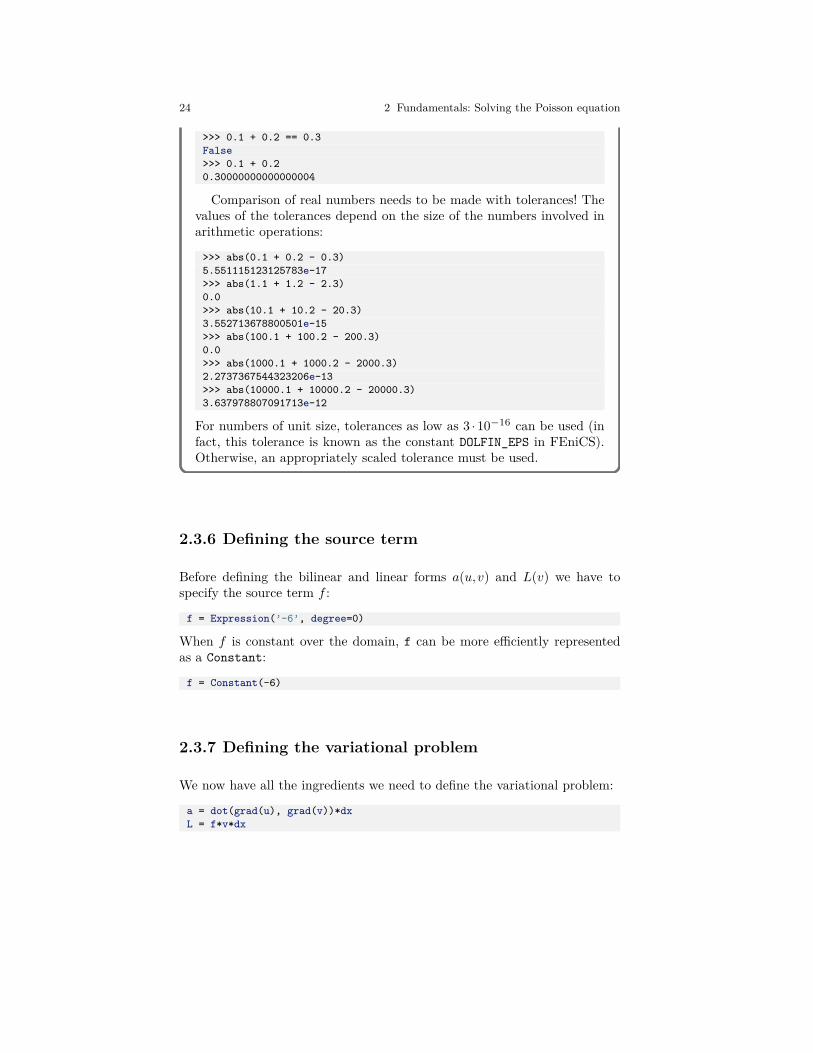
24 2 Fundamentals: Solving the Poisson equation
>>> 0.1 + 0.2 == 0.3False>>> 0.1 + 0.20.30000000000000004
Comparison of real numbers needs to be made with tolerances! Thevalues of the tolerances depend on the size of the numbers involved inarithmetic operations:
>>> abs(0.1 + 0.2 - 0.3)5.551115123125783e-17>>> abs(1.1 + 1.2 - 2.3)0.0>>> abs(10.1 + 10.2 - 20.3)3.552713678800501e-15>>> abs(100.1 + 100.2 - 200.3)0.0>>> abs(1000.1 + 1000.2 - 2000.3)2.2737367544323206e-13>>> abs(10000.1 + 10000.2 - 20000.3)3.637978807091713e-12
For numbers of unit size, tolerances as low as 3 ·10−16 can be used (infact, this tolerance is known as the constant DOLFIN_EPS in FEniCS).Otherwise, an appropriately scaled tolerance must be used.
2.3.6 Defining the source term
Before defining the bilinear and linear forms a(u,v) and L(v) we have tospecify the source term f :
f = Expression(’-6’, degree=0)
When f is constant over the domain, f can be more efficiently representedas a Constant:
f = Constant(-6)
2.3.7 Defining the variational problem
We now have all the ingredients we need to define the variational problem:
a = dot(grad(u), grad(v))*dxL = f*v*dx
2.3 Dissection of the program 25
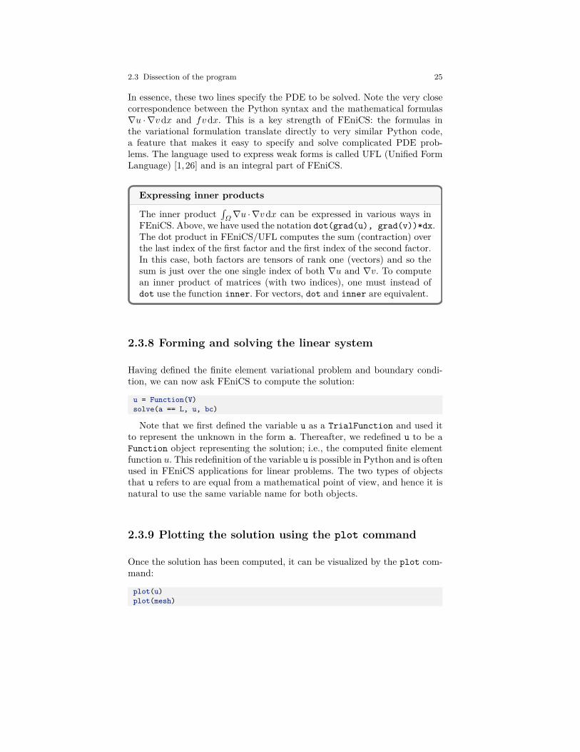
In essence, these two lines specify the PDE to be solved. Note the very closecorrespondence between the Python syntax and the mathematical formulas∇u · ∇vdx and fvdx. This is a key strength of FEniCS: the formulas inthe variational formulation translate directly to very similar Python code,a feature that makes it easy to specify and solve complicated PDE prob-lems. The language used to express weak forms is called UFL (Unified FormLanguage) [1, 26] and is an integral part of FEniCS.
Expressing inner products
The inner product∫Ω∇u ·∇vdx can be expressed in various ways in
FEniCS. Above, we have used the notation dot(grad(u), grad(v))*dx.The dot product in FEniCS/UFL computes the sum (contraction) overthe last index of the first factor and the first index of the second factor.In this case, both factors are tensors of rank one (vectors) and so thesum is just over the one single index of both ∇u and ∇v. To computean inner product of matrices (with two indices), one must instead ofdot use the function inner. For vectors, dot and inner are equivalent.
2.3.8 Forming and solving the linear system
Having defined the finite element variational problem and boundary condi-tion, we can now ask FEniCS to compute the solution:
u = Function(V)solve(a == L, u, bc)
Note that we first defined the variable u as a TrialFunction and used itto represent the unknown in the form a. Thereafter, we redefined u to be aFunction object representing the solution; i.e., the computed finite elementfunction u. This redefinition of the variable u is possible in Python and is oftenused in FEniCS applications for linear problems. The two types of objectsthat u refers to are equal from a mathematical point of view, and hence it isnatural to use the same variable name for both objects.
2.3.9 Plotting the solution using the plot command
Once the solution has been computed, it can be visualized by the plot com-mand:
plot(u)plot(mesh)

26 2 Fundamentals: Solving the Poisson equation
interactive()
Note the call to the function interactive after the plot commands. Thiscall makes it possible to interact with the plots (rotating and zooming). Thecall to interactive is usually placed at the end of a program that createsplots. Figure 2.1 displays the two plots.
Fig. 2.1 Plot of the mesh and the solution for the Poisson problem created using thebuilt-in FEniCS visualization tool (plot command).
The plot command is useful for debugging and initial scientific investi-gations. More advanced visualizations are better created by exporting thesolution to a file and using an advanced visualization tool like ParaView, asexplained in the next section.
By clicking the left mouse button in the plot window, you may rotate thesolution, while the right mouse button is used for zooming. Point the mouse tothe Help text in the lower left corner to display a list of all available shortcutcommands. The help menu may alternatively be activated by typing h inthe plot window. The plot command also accepts a number of additionalarguments, such as for example setting the title of the plot window:
plot(u, title=’Finite element solution’)plot(mesh, title=’Finite element mesh’)
For detailed documentation, either run the command help(plot) in Pythonor pydoc fenics.plot from a terminal window.
Built-in plotting on Mac OS X and in Docker
The built-in plotting in FEniCS may not work as expected when eitherrunning on Mac OS X or when running inside a FEniCS Docker con-tainer. FEniCS supports plotting using the plot command on Mac OSX. However, the keyboard shortcuts may fail to work. When running

2.3 Dissection of the program 27
inside a Docker container, plotting is not supported since Docker doesnot interact with your windowing system. For Docker users who needplotting, it is recommended to either work within a Jupyter/FEniCSnotebook (command fenicsproject notebook) or rely on ParaViewor other external tools for visualization.
2.3.10 Plotting the solution using ParaView
The simple plot command is useful for quick visualizations, but for moreadvanced visualizations an external tool must be used. In this section wedemonstrate how to visualize solutions in ParaView. ParaView3 is a powerfultool for visualizing scalar and vector fields, including those computed byFEniCS.
The first step is to export the solution in VTK format:
vtkfile = File(’poisson/solution.pvd’)vtkfile << u
The following steps demonstrate how to create a plot of the solution of ourPoisson problem in ParaView. The resulting plot is shown in Figure 2.2.
1. Start the ParaView application.2. Click File–Open... in the top menu and navigate to the directory con-
taining the exported solution. This should be inside a subdirectory namedpoisson below the directory where the FEniCS Python program wasstarted. Select the file named solution.pvd and then click OK.
3. Click Apply in the Properties pane on the left. This will bring up a plotof the solution.
4. To make a 3D plot of the solution, we will make use of one of ParaView’smany filters. Click Filters–Alphabetical–Warp By Scalar in the topmenu and then Apply in the Properties pane on the left. This create anelevated surface with the height determined by the solution value.
5. To show the original plot below the elevated surface, click the little eyeicon to the left of solution.pvd in the Pipeline Browser pane on the left.Also click the little 2D button at the top of the plot window to change thevisualization to 3D. This lets you interact with the plot by rotating (leftmouse button) and zooming (Ctrl + left mouse button).
6. To show the finite element mesh, click on solution.pvd in the PipelineBrowser, navigate to Representation in the Properties pane, and selectSurface With Edges. This should make the finite element mesh visible.
7. To change the aspect ratio of the plot, click on WarpByScalar1 in thePipeline Browser and navigate to Scale Factor in the Properties pane.Change the value to 0.2 and click Apply. This will change the scale of the
3http://www.paraview.org

28 2 Fundamentals: Solving the Poisson equation
warped plot. We also unclick Orientation Axis Visibility at the bottomof the Properties pane to remove the little 3D axes in the lower left cornerof the plot window. You should now see something that resembles the plotin Figure 2.2.
8. Finally, to export the visualization to a file, click File–Save Screen-shot... and select a suitable file name such as poisson.png.
For more information, we refer to The ParaView Guide [30] (free PDF avail-able), the ParaView tutorial4, and the instruction video Introduction to Par-aView5.
Fig. 2.2 Plot of the mesh and the solution for the Poisson problem created usingParaView.
2.3.11 Computing the error
Finally, we compute the error to check the accuracy of the solution. We dothis by comparing the finite element solution u with the exact solution, whichin this example happens to be the same as the expression u_D used to set theboundary conditions. We compute the error in two different ways. First, wecompute the L2 norm of the error, defined by
4http://www.paraview.org/Wiki/The_ParaView_Tutorial5https://vimeo.com/34037236

2.3 Dissection of the program 29
E =
√∫Ω
(uD −u)2 dx.
Since the exact solution is quadratic and the finite element solution is piece-wise linear, this error will be nonzero. To compute this error in FEniCS, wesimply write
error_L2 = errornorm(u_D, u, ’L2’)
The errornorm function can also compute other error norms such as the H1
norm. Type pydoc fenics.errornorm in a terminal window for details.We also compute the maximum value of the error at all the vertices of the
finite element mesh. As mentioned above, we expect this error to be zero towithin machine precision for this particular example. To compute the errorat the vertices, we first ask FEniCS to compute the value of both u_D and uat all vertices, and then subtract the results:
vertex_values_u_D = u_D.compute_vertex_values(mesh)vertex_values_u = u.compute_vertex_values(mesh)import numpy as nperror_max = np.max(np.abs(vertex_values_u_D - vertex_values_u))
We have here used the maximum and absolute value functions from numpy,because these are much more efficient for large arrays (a factor of 30) thanPython’s built-in max and abs functions.
How to check that the error vanishes
With inexact (floating point) arithmetic, the maximum error at the ver-tices is not zero, but should be a small number. The machine precision isabout 10−16, but in finite element calculations, rounding errors of thissize may accumulate, to produce an error larger than 10−16. Experi-ments show that increasing the number of elements and increasing thedegree of the finite element polynomials increases the error. For a meshwith 2×(20×20) cubic Lagrange elements (degree 3) the error is about2 ·10−12, while for 128 linear elements the error is about 2 ·10−15.
2.3.12 Examining degrees of freedom and vertex values
A finite element function like u is expressed as a linear combination of basisfunctions φj , spanning the space V :
u=N∑j=1
Ujφj . (2.13)

30 2 Fundamentals: Solving the Poisson equation
By writing solve(a == L, u, bc) in the program, a linear system will beformed from a and L, and this system is solved for the values U1, . . . ,UN .The values U1, . . . ,UN are known as the degrees of freedom (“dofs”) or nodalvalues of u. For Lagrange elements (and many other element types) Uj issimply the value of u at the node with global number j. The locations ofthe nodes and cell vertices coincide for linear Lagrange elements, while forhigher-order elements there are additional nodes associated with the facets,edges and sometimes also the interior of cells.
Having u represented as a Function object, we can either evaluate u(x)at any point x in the mesh (expensive operation!), or we can grab all thedegrees of freedom in the vector U directly by
nodal_values_u = u.vector()
The result is a Vector object, which is basically an encapsulation of thevector object used in the linear algebra package that is used to solve the linearsystem arising from the variational problem. Since we program in Python itis convenient to convert the Vector object to a standard numpy array forfurther processing:
array_u = nodal_values_u.array()
With numpy arrays we can write MATLAB-like code to analyze the data.Indexing is done with square brackets: array_u[j], where the index j al-ways starts at 0. If the solution is computed with piecewise linear Lagrangeelements (P1), then the size of the array array_u is equal to the number ofvertices, and each array_u[j] is the value at some vertex in the mesh. How-ever, the degrees of freedom are not necessarily numbered in the same way asthe vertices of the mesh. (This is discussed in some detail in Section 5.4.1).If we therefore want to know the values at the vertices, we need to call thefunction u.compute_vertex_values. This function returns the values at allthe vertices of the mesh as a numpy array with the same numbering as forthe vertices of the mesh, for example:
vertex_values_u = u.compute_vertex_values()
Note that for P1 elements, the arrays array_u and vertex_values_u havethe same lengths and contain the same values, albeit in different order.
2.4 Deflection of a membrane
Our first FEniCS program for the Poisson equation targeted a simple testproblem where we could easily verify the implementation. We now turn ourattention to a physically more relevant problem with solutions of somewhatmore exciting shape.

2.4 Deflection of a membrane 31
We want to compute the deflection D(x,y) of a two-dimensional, circularmembrane of radius R, subject to a load p over the membrane. The appro-priate PDE model is
−T∇2D = p in Ω = (x,y) |x2 +y2 ≤R . (2.14)
Here, T is the tension in the membrane (constant), and p is the externalpressure load. The boundary of the membrane has no deflection, implyingD= 0 as a boundary condition. A localized load can be modeled as a Gaussianfunction:
p(x,y) = A
2πσ exp(−1
2
(x−x0σ
)2− 1
2
(y−y0σ
)2). (2.15)
The parameter A is the amplitude of the pressure, (x0,y0) the localizationof the maximum point of the load, and σ the “width” of p. We will take thecenter (x0,y0) of the pressure to be (0,R0) for some 0<R0 <R.
2.4.1 Scaling the equation
There are many physical parameters in this problem, and we can benefitfrom grouping them by means of scaling. Let us introduce dimensionlesscoordinates x = x/R, y = y/R, and a dimensionless deflection w = D/Dc,where Dc is a characteristic size of the deflection. Introducing R0 = R0/R,we obtain
−∂2w
∂x2 −∂2w
∂y2 = αexp(−β2(x2 + (y− R0)2)
)for x2 + y2 < 1,
where
α= R2A
2πTDcσ, β = R√
2σ.
With an appropriate scaling, w and its derivatives are of size unity, so theleft-hand side of the scaled PDE is about unity in size, while the right-handside has α as its characteristic size. This suggest choosing α to be unity,or around unity. We shall in this particular case choose α = 4. (One canalso find the analytical solution in scaled coordinates and show that themaximum deflection D(0,0) is Dc if we choose α= 4 to determine Dc.) WithDc =AR2/(8πσT ) and dropping the bars we obtain the scaled problem
−∇2w = 4exp(−β2(x2 + (y−R0)2)
), (2.16)
to be solved over the unit disc with w = 0 on the boundary. Now there areonly two parameters to vary: the dimensionless extent of the pressure, β, and
32 2 Fundamentals: Solving the Poisson equation
the localization of the pressure peak, R0 ∈ [0,1]. As β→ 0, the solution willapproach the special case w = 1−x2−y2.
Given a computed scaled solution w, the physical deflection can be com-puted by
D = AR2
8πσT w.
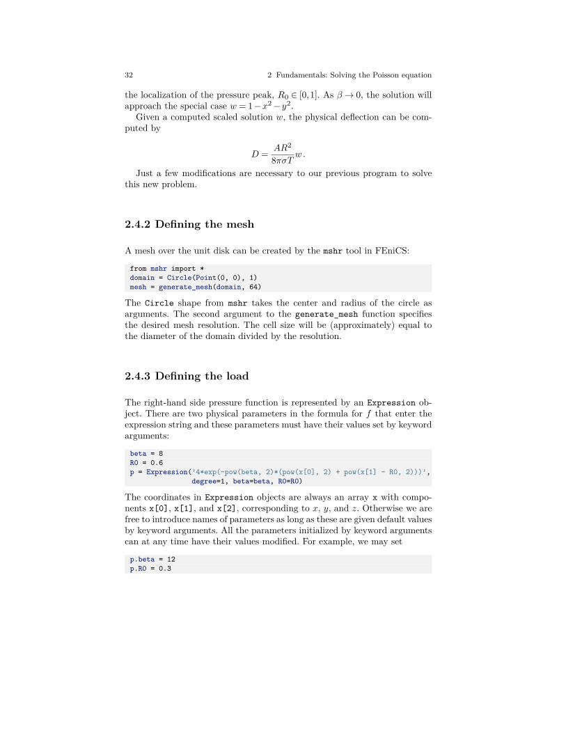
Just a few modifications are necessary to our previous program to solvethis new problem.
2.4.2 Defining the mesh
A mesh over the unit disk can be created by the mshr tool in FEniCS:
from mshr import *domain = Circle(Point(0, 0), 1)mesh = generate_mesh(domain, 64)
The Circle shape from mshr takes the center and radius of the circle asarguments. The second argument to the generate_mesh function specifiesthe desired mesh resolution. The cell size will be (approximately) equal tothe diameter of the domain divided by the resolution.
2.4.3 Defining the load
The right-hand side pressure function is represented by an Expression ob-ject. There are two physical parameters in the formula for f that enter theexpression string and these parameters must have their values set by keywordarguments:
beta = 8R0 = 0.6p = Expression(’4*exp(-pow(beta, 2)*(pow(x[0], 2) + pow(x[1] - R0, 2)))’,
degree=1, beta=beta, R0=R0)
The coordinates in Expression objects are always an array x with compo-nents x[0], x[1], and x[2], corresponding to x, y, and z. Otherwise we arefree to introduce names of parameters as long as these are given default valuesby keyword arguments. All the parameters initialized by keyword argumentscan at any time have their values modified. For example, we may set
p.beta = 12p.R0 = 0.3
2.4 Deflection of a membrane 33
2.4.4 Defining the variational problem
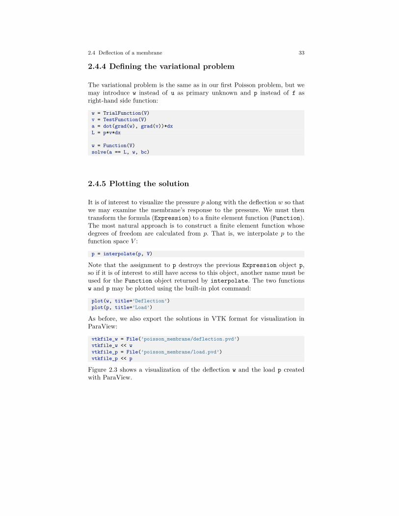
The variational problem is the same as in our first Poisson problem, but wemay introduce w instead of u as primary unknown and p instead of f asright-hand side function:
w = TrialFunction(V)v = TestFunction(V)a = dot(grad(w), grad(v))*dxL = p*v*dx
w = Function(V)solve(a == L, w, bc)
2.4.5 Plotting the solution
It is of interest to visualize the pressure p along with the deflection w so thatwe may examine the membrane’s response to the pressure. We must thentransform the formula (Expression) to a finite element function (Function).The most natural approach is to construct a finite element function whosedegrees of freedom are calculated from p. That is, we interpolate p to thefunction space V :
p = interpolate(p, V)
Note that the assignment to p destroys the previous Expression object p,so if it is of interest to still have access to this object, another name must beused for the Function object returned by interpolate. The two functionsw and p may be plotted using the built-in plot command:
plot(w, title=’Deflection’)plot(p, title=’Load’)
As before, we also export the solutions in VTK format for visualization inParaView:
vtkfile_w = File(’poisson_membrane/deflection.pvd’)vtkfile_w << wvtkfile_p = File(’poisson_membrane/load.pvd’)vtkfile_p << p
Figure 2.3 shows a visualization of the deflection w and the load p createdwith ParaView.

34 2 Fundamentals: Solving the Poisson equation
Fig. 2.3 Plot of the deflection (left) and load (right) for the membrane problem createdusing ParaView. The plot uses 10 equispaced isolines for the solution values and theoptional jet colormap.
2.4.6 Making curve plots through the domain
Another way to compare the deflection and the load is to make a curve plotalong the line x= 0. This is just a matter of defining a set of points along they-axis and evaluating the finite element functions w and p at these points:
# Curve plot along x = 0 comparing p and wimport numpy as npimport matplotlib.pyplot as plttol = 0.001 # avoid hitting points outside the domainy = np.linspace(-1 + tol, 1 - tol, 101)points = [(0, y_) for y_ in y] # 2D pointsw_line = np.array([w(point) for point in points])p_line = np.array([p(point) for point in points])plt.plot(y, 50*w_line, ’k’, linewidth=2) # magnify wplt.plot(y, p_line, ’b--’, linewidth=2)plt.grid(True)plt.xlabel(’$y$’)plt.legend([’Deflection ($\\times 50$)’, ’Load’], loc=’upper left’)plt.savefig(’poisson_membrane/curves.pdf’)plt.savefig(’poisson_membrane/curves.png’)
This example program can be found in the file ft02_poisson_membrane.py.The resulting curve plot is shown in Figure 2.4. The localized input (p)
is heavily damped and smoothed in the output (w). This reflects a typicalproperty of the Poisson equation.

2.4 Deflection of a membrane 35
Fig. 2.4 Plot of the deflection and load for the membrane problem created usingMatplotlib and sampling of the two functions along the y-axsis.

Chapter 3A Gallery of finite element solvers
The goal of this chapter is to demonstrate how a range of important PDEs fromscience and engineering can be quickly solved with a few lines of FEniCS code.We start with the heat equation and continue with a nonlinear Poisson equation,the equations for linear elasticity, the Navier–Stokes equations, and finally look athow to solve systems of nonlinear advection–diffusion–reaction equations. Theseproblems illustrate how to solve time-dependent problems, nonlinear problems,vector-valued problems, and systems of PDEs. For each problem, we derive thevariational formulation and express the problem in Python in a way that closelyresembles the mathematics.
3.1 The heat equation
As a first extension of the Poisson problem from the previous chapter, weconsider the time-dependent heat equation, or the time-dependent diffusionequation. This is the natural extension of the Poisson equation describing thestationary distribution of heat in a body to a time-dependent problem.
We will see that by discretizing time into small time intervals and applyingstandard time-stepping methods, we can solve the heat equation by solvinga sequence of variational problems, much like the one we encountered for thePoisson equation.
3.1.1 PDE problem
Our model problem for time-dependent PDEs reads
c© 2017, Hans Petter Langtangen, Anders Logg.Released under CC Attribution 4.0 license

38 3 A Gallery of finite element solvers
∂u
∂t=∇2u+f in Ω× (0,T ], (3.1)
u= uD on ∂Ω× (0,T ], (3.2)u= u0 at t= 0 . (3.3)
Here, u varies with space and time, e.g., u= u(x,y, t) if the spatial domain Ωis two-dimensional. The source function f and the boundary values uD mayalso vary with space and time. The initial condition u0 is a function of spaceonly.
3.1.2 Variational formulation
A straightforward approach to solving time-dependent PDEs by the finiteelement method is to first discretize the time derivative by a finite differenceapproximation, which yields a sequence of stationary problems, and then turneach stationary problem into a variational formulation.
Let superscript n denote a quantity at time tn, where n is an integer count-ing time levels. For example, un means u at time level n. A finite differencediscretization in time first consists of sampling the PDE at some time level,say tn+1: (
∂u
∂t
)n+1=∇2un+1 +fn+1 . (3.4)
The time-derivative can be approximated by a difference quotient. For sim-plicity and stability reasons, we choose a simple backward difference:(
∂u
∂t
)n+1≈ un+1−un
∆t, (3.5)
where ∆t is the time discretization parameter. Inserting (3.5) in (3.4) yields
un+1−un
∆t=∇2un+1 +fn+1 . (3.6)
This is our time-discrete version of the heat equation (3.1), a so-called back-ward Euler or implicit Euler discretization.
We may reorder (3.6) so that the left-hand side contains the terms withthe unknown un+1 and the right-hand side contains computed terms only.The result is a sequence of spatial (stationary) problems for un+1, assumingun is known from the previous time step:
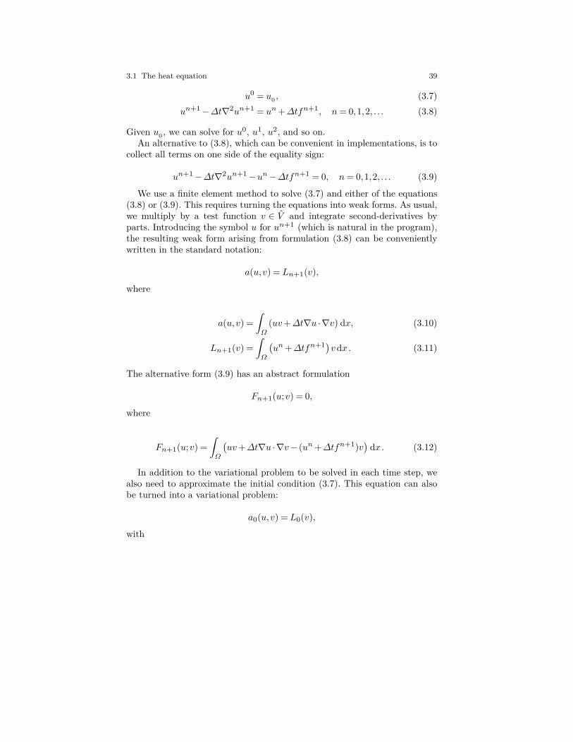
3.1 The heat equation 39
u0 = u0 , (3.7)un+1−∆t∇2un+1 = un+∆tfn+1, n= 0,1,2, . . . (3.8)
Given u0 , we can solve for u0, u1, u2, and so on.An alternative to (3.8), which can be convenient in implementations, is to
collect all terms on one side of the equality sign:
un+1−∆t∇2un+1−un−∆tfn+1 = 0, n= 0,1,2, . . . (3.9)
We use a finite element method to solve (3.7) and either of the equations(3.8) or (3.9). This requires turning the equations into weak forms. As usual,we multiply by a test function v ∈ V and integrate second-derivatives byparts. Introducing the symbol u for un+1 (which is natural in the program),the resulting weak form arising from formulation (3.8) can be convenientlywritten in the standard notation:
a(u,v) = Ln+1(v),
where
a(u,v) =∫Ω
(uv+∆t∇u ·∇v) dx, (3.10)
Ln+1(v) =∫Ω
(un+∆tfn+1)vdx. (3.11)
The alternative form (3.9) has an abstract formulation
Fn+1(u;v) = 0,
where
Fn+1(u;v) =∫Ω
(uv+∆t∇u ·∇v− (un+∆tfn+1)v
)dx. (3.12)
In addition to the variational problem to be solved in each time step, wealso need to approximate the initial condition (3.7). This equation can alsobe turned into a variational problem:
a0(u,v) = L0(v),
with

40 3 A Gallery of finite element solvers
a0(u,v) =∫Ωuvdx, (3.13)
L0(v) =∫Ωu0vdx. (3.14)
When solving this variational problem, u0 becomes the L2 projection of thegiven initial value u0 into the finite element space. The alternative is to con-struct u0 by just interpolating the initial value u0 ; that is, if u0 =
∑Nj=1U
0j φj ,
we simply set Uj = u0(xj ,yj), where (xj ,yj) are the coordinates of node num-ber j. We refer to these two strategies as computing the initial condition byeither projection or interpolation. Both operations are easy to compute inFEniCS through a single statement, using either the project or interpolatefunction. The most common choice is project, which computes an approxi-mation to u0 , but in some applications where we want to verify the code byreproducing exact solutions, one must use interpolate (and we use such atest problem here!).
In summary, we thus need to solve the following sequence of variationalproblems to compute the finite element solution to the heat equation: findu0 ∈ V such that a0(u0,v) =L0(v) holds for all v ∈ V , and then find un+1 ∈ Vsuch that a(un+1,v) =Ln+1(v) for all v ∈ V , or alternatively, Fn+1(un+1,v) =0 for all v ∈ V , for n= 0,1,2, . . ..
3.1.3 FEniCS implementation
Our program needs to implement the time-stepping manually, but can relyon FEniCS to easily compute a0, L0, a, and L (or Fn+1), and solve the linearsystems for the unknowns.
Test problem 1: A known analytical solution. Just as for the Poissonproblem from the previous chapter, we construct a test problem that makesit easy to determine if the calculations are correct. Since we know that ourfirst-order time-stepping scheme is exact for linear functions, we create atest problem which has a linear variation in time. We combine this with aquadratic variation in space. We thus take
u= 1 +x2 +αy2 +βt, (3.15)
which yields a function whose computed values at the nodes will be exact,regardless of the size of the elements and ∆t, as long as the mesh is uniformlypartitioned. By inserting (3.15) into the heat equation (3.1), we find that theright-hand side f must be given by f(x,y, t) = β−2−2α. The boundary valueis uD(x,y, t) = 1+x2 +αy2 +βt and the initial value is u0(x,y) = 1+x2 +αy2.
FEniCS implementation. A new programming issue is how to dealwith functions that vary in space and time, such as the boundary condi-

3.1 The heat equation 41
tion uD(x,y, t) = 1 + x2 +αy2 + βt. A natural solution is to use a FEniCSExpression with time t as a parameter, in addition to the parameters α andβ:
alpha = 3; beta = 1.2u_D = Expression(’1 + x[0]*x[0] + alpha*x[1]*x[1] + beta*t’,
degree=2, alpha=alpha, beta=beta, t=0)
This Expression uses the components of x as independent variables, whilealpha, beta, and t are parameters. The time t can later be updated by
u_D.t = t
The essential boundary conditions, along the entire boundary in this case,are implemented in the same way as we have previously implemented theboundary conditions for the Poisson problem:
def boundary(x, on_boundary):return on_boundary
bc = DirichletBC(V, u_D, boundary)
We shall use the variable u for the unknown un+1 at the new time stepand the variable u_n for un at the previous time step. The initial value ofu_n can be computed by either projection or interpolation of u0 . Since weset t = 0 for the boundary value u_D, we can use u_D to specify the initialcondition:
u_n = project(u_D, V)# oru_n = interpolate(u_D, V)
Projecting versus interpolating the initial condition
To actually recover the exact solution (3.15) to machine precision, it isimportant to compute the discrete initial condition by interpolating u0 .This ensures that the degrees of freedom are exact (to machine preci-sion) at t= 0. Projection results in approximate values at the nodes.
We may either define a or L according to the formulas above, or we mayjust define F and ask FEniCS to figure out which terms should go into thebilinear form a and which should go into the linear form L. The latter isconvenient, especially in more complicated problems, so we illustrate thatconstruction of a and L:
u = TrialFunction(V)v = TestFunction(V)f = Constant(beta - 2 - 2*alpha)
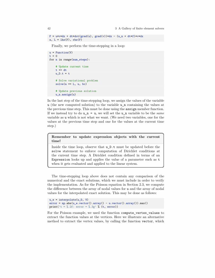
42 3 A Gallery of finite element solvers
F = u*v*dx + dt*dot(grad(u), grad(v))*dx - (u_n + dt*f)*v*dxa, L = lhs(F), rhs(F)
Finally, we perform the time-stepping in a loop:
u = Function(V)t = 0for n in range(num_steps):
# Update current timet += dtu_D.t = t
# Solve variational problemsolve(a == L, u, bc)
# Update previous solutionu_n.assign(u)
In the last step of the time-stepping loop, we assign the values of the variableu (the new computed solution) to the variable u_n containing the values atthe previous time step. This must be done using the assign member function.If we instead try to do u_n = u, we will set the u_n variable to be the samevariable as u which is not what we want. (We need two variables, one for thevalues at the previous time step and one for the values at the current timestep.)
Remember to update expression objects with the currenttime!Inside the time loop, observe that u_D.t must be updated before thesolve statement to enforce computation of Dirichlet conditions atthe current time step. A Dirichlet condition defined in terms of anExpression looks up and applies the value of a parameter such as twhen it gets evaluated and applied to the linear system.
The time-stepping loop above does not contain any comparison of thenumerical and the exact solutions, which we must include in order to verifythe implementation. As for the Poisson equation in Section 2.3, we computethe difference between the array of nodal values for u and the array of nodalvalues for the interpolated exact solution. This may be done as follows:
u_e = interpolate(u_D, V)error = np.abs(u_e.vector().array() - u.vector().array()).max()print(’t = %.2f: error = %.3g’ % (t, error))
For the Poisson example, we used the function compute_vertex_values toextract the function values at the vertices. Here we illustrate an alternativemethod to extract the vertex values, by calling the function vector, which

3.1 The heat equation 43
returns the vector of degrees of freedom. For a P1 function space, this vectorof degrees of freedom will be equal to the array of vertex values obtained bycalling compute_vertex_values, albeit possibly in a different order.
The complete program for solving the heat equation goes as follows:
from fenics import *import numpy as np
T = 2.0 # final timenum_steps = 10 # number of time stepsdt = T / num_steps # time step sizealpha = 3 # parameter alphabeta = 1.2 # parameter beta
# Create mesh and define function spacenx = ny = 8mesh = UnitSquareMesh(nx, ny)V = FunctionSpace(mesh, ’P’, 1)
# Define boundary conditionu_D = Expression(’1 + x[0]*x[0] + alpha*x[1]*x[1] + beta*t’,
degree=2, alpha=alpha, beta=beta, t=0)
def boundary(x, on_boundary):return on_boundary
bc = DirichletBC(V, u_D, boundary)
# Define initial valueu_n = interpolate(u_D, V)#u_n = project(u_D, V)
# Define variational problemu = TrialFunction(V)v = TestFunction(V)f = Constant(beta - 2 - 2*alpha)
F = u*v*dx + dt*dot(grad(u), grad(v))*dx - (u_n + dt*f)*v*dxa, L = lhs(F), rhs(F)
# Time-steppingu = Function(V)t = 0for n in range(num_steps):
# Update current timet += dtu_D.t = t
# Compute solutionsolve(a == L, u, bc)
# Plot solution

44 3 A Gallery of finite element solvers
plot(u)
# Compute error at verticesu_e = interpolate(u_D, V)error = np.abs(u_e.vector().array() - u.vector().array()).max()print(’t = %.2f: error = %.3g’ % (t, error))
# Update previous solutionu_n.assign(u)
# Hold plotinteractive()
This example program can be found in the file ft03_heat.py.
Test problem 2: Diffusion of a Gaussian function. Let us now solvea more interesting test problem, namely the diffusion of a Gaussian hill. Wetake the initial value to be
u0(x,y) = e−ax2−ay2
for a= 5 on the domain [−2,2]× [2,2]. For this problem we will use homoge-neous Dirichlet boundary conditions (uD = 0).
FEniCS implementation. Which are the required changes to our previousprogram? One major change is that the domain is no longer a unit square.The new domain can be created easily in FEniCS using RectangleMesh:
nx = ny = 30mesh = RectangleMesh(Point(-2, -2), Point(2, 2), nx, ny)
Note that we have used a much higher resolution than before to better re-solve the features of the solution. We also need to redefine the initial condi-tion and the boundary condition. Both are easily changed by defining a newExpression and by setting u= 0 on the boundary.
To be able to visualize the solution in an external program such as Par-aView, we will save the solution to a file in VTK format in each time step.We do this by first creating a File with the suffix .pvd:
vtkfile = File(’heat_gaussian/solution.pvd’)
Inside the time loop, we may then append the solution values to this file:
vtkfile << (u, t)
This line is called in each time step, resulting in the creation of a new filewith suffix .vtu containing all data for the time step (the mesh and thevertex values). The file heat_gaussian/solution.pvd will contain the timevalues and references to the .vtu file, which means that the .pvd file willbe a single small file that points to a large number of .vtu files containingthe actual data. Note that we choose to store the solution to a subdirectorynamed heat_gaussian. This is to avoid cluttering our source directory with
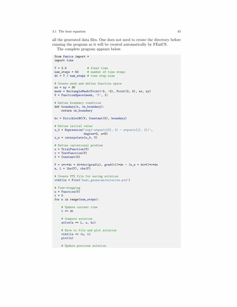
3.1 The heat equation 45
all the generated data files. One does not need to create the directory beforerunning the program as it will be created automatically by FEniCS.
The complete program appears below.
from fenics import *import time
T = 2.0 # final timenum_steps = 50 # number of time stepsdt = T / num_steps # time step size
# Create mesh and define function spacenx = ny = 30mesh = RectangleMesh(Point(-2, -2), Point(2, 2), nx, ny)V = FunctionSpace(mesh, ’P’, 1)
# Define boundary conditiondef boundary(x, on_boundary):
return on_boundary
bc = DirichletBC(V, Constant(0), boundary)
# Define initial valueu_0 = Expression(’exp(-a*pow(x[0], 2) - a*pow(x[1], 2))’,
degree=2, a=5)u_n = interpolate(u_0, V)
# Define variational problemu = TrialFunction(V)v = TestFunction(V)f = Constant(0)
F = u*v*dx + dt*dot(grad(u), grad(v))*dx - (u_n + dt*f)*v*dxa, L = lhs(F), rhs(F)
# Create VTK file for saving solutionvtkfile = File(’heat_gaussian/solution.pvd’)
# Time-steppingu = Function(V)t = 0for n in range(num_steps):
# Update current timet += dt
# Compute solutionsolve(a == L, u, bc)
# Save to file and plot solutionvtkfile << (u, t)plot(u)
# Update previous solution

46 3 A Gallery of finite element solvers
u_n.assign(u)
# Hold plotinteractive()
This example program can be found in the file ft04_heat_gaussian.py.Visualization in ParaView. To visualize the diffusion of the Gaussian hill,start ParaView, choose File–Open..., open heat_gaussian/solution.pvd,and click Apply in the Properties pane. Click on the play button to displayan animation of the solution. To save the animation to a file, click File–Save Animation... and save the file to a desired file format, for exampleAVI or Ogg/Theora. Once the animation has been saved to a file, you canplay the animation offline using a player such as mplayer or VLC, or uploadyour animation to YouTube. Figure 3.1 shows a sequence of snapshots of thesolution.
Fig. 3.1 A sequence of snapshots of the solution of the Gaussian hill problem createdwith ParaView.
3.2 A nonlinear Poisson equation
We shall now address how to solve nonlinear PDEs. We will see that nonlinearproblems can be solved just as easily as linear problems in FEniCS, by sim-ply defining a nonlinear variational problem and calling the solve function.When doing so, we will encounter a subtle difference in how the variationalproblem is defined.
3.2.1 PDE problem
As a model problem for the solution of nonlinear PDEs, we take the followingnonlinear Poisson equation:
3.2 A nonlinear Poisson equation 47
−∇· (q(u)∇u) = f, (3.16)
in Ω, with u = uD on the boundary ∂Ω. The coefficient q = q(u) makes theequation nonlinear (unless q(u) is constant in u).
3.2.2 Variational formulation
As usual, we multiply our PDE by a test function v ∈ V , integrate over thedomain, and integrate the second-order derivatives by parts. The bound-ary integral arising from integration by parts vanishes wherever we employDirichlet conditions. The resulting variational formulation of our model prob-lem becomes: find u ∈ V such that
F (u;v) = 0 ∀v ∈ V , (3.17)
where
F (u;v) =∫Ω
(q(u)∇u ·∇v−fv)dx, (3.18)
and
V = v ∈H1(Ω) : v = uD on ∂Ω,V = v ∈H1(Ω) : v = 0 on ∂Ω .
The discrete problem arises as usual by restricting V and V to a pairof discrete spaces. As before, we omit any subscript on the discrete spacesand discrete solution. The discrete nonlinear problem is then written as: findu ∈ V such that
F (u;v) = 0 ∀v ∈ V , (3.19)
with u=∑Nj=1Ujφj . Since F is nonlinear in u, the variational statement gives
rise to a system of nonlinear algebraic equations in the unknowns U1, . . . ,UN .
3.2.3 FEniCS implementation
Test problem. To solve a test problem, we need to choose the right-handside f , the coefficient q(u) and the boundary value uD . Previously, we haveworked with manufactured solutions that can be reproduced without approx-imation errors. This is more difficult in nonlinear problems, and the algebra

48 3 A Gallery of finite element solvers
is more tedious. However, we may utilize SymPy for symbolic computing andintegrate such computations in the FEniCS solver. This allows us to eas-ily experiment with different manufactured solutions. The forthcoming codewith SymPy requires some basic familiarity with this package. In particular,we will use the SymPy functions diff for symbolic differentiation and ccodefor C/C++ code generation.
We take q(u) = 1+u2 and define a two-dimensional manufactured solutionthat is linear in x and y:
# Warning: from fenics import * will import both ‘sym‘ and# ‘q‘ from FEniCS. We therefore import FEniCS first and then# overwrite these objects.from fenics import *
def q(u):"Return nonlinear coefficient"return 1 + u**2
# Use SymPy to compute f from the manufactured solution uimport sympy as symx, y = sym.symbols(’x[0], x[1]’)u = 1 + x + 2*yf = - sym.diff(q(u)*sym.diff(u, x), x) - sym.diff(q(u)*sym.diff(u, y), y)f = sym.simplify(f)u_code = sym.printing.ccode(u)f_code = sym.printing.ccode(f)print(’u =’, u_code)print(’f =’, f_code)
Define symbolic coordinates as required in Expression objects
Note that we would normally write x, y = sym.symbols(’x, y’), butif we want the resulting expressions to have valid syntax for FEniCSExpression objects, we must use x[0] and x[1]. This is easily accom-plished with sympy by defining the names of x and y as x[0] and x[1]:x, y = sym.symbols(’x[0], x[1]’).
Turning the expressions for u and f into C or C++ syntax for FEniCSExpression objects needs two steps. First, we ask for the C code of theexpressions:
u_code = sym.printing.ccode(u)f_code = sym.printing.ccode(f)
In some cases, one will need to edit the result to match the required syntaxof Expression objects, but not in this case. (The primary example is thatM_PI for π in C/C++ must be replaced by pi for Expression objects.) Inthe present case, the output of u_code and f_code is

3.2 A nonlinear Poisson equation 49
x[0] + 2*x[1] + 1-10*x[0] - 20*x[1] - 10
After having defined the mesh, the function space, and the boundary, wedefine the boundary value u_D as
u_D = Expression(u_code, degree=1)
Similarly, we define the right-hand side function as
f = Expression(f_code, degree=1)
Name clash between FEniCS and program variables
In a program like the one above, strange errors may occur due to nameclashes. If you define sym and q prior to doing from fenics import *,the latter statement will also import variables with the names sym andq, overwriting the objects you have previously defined! This may leadto strange errors. The safest solution is to do import fenics insteadof from fenics import * and then prefix all FEniCS object names byfenics. The next best solution is to do from fenics import * firstand then define your own variables that overwrite those imported fromfenics. This is acceptable if we do not need sym and q from fenics.
FEniCS implementation. A solver for the nonlinear Poisson equation isas easy to implement as a solver for the linear Poisson equation. All we needto do is to state the formula for F and call solve(F == 0, u, bc) insteadof solve(a == L, u, bc) as we did in the linear case. Here is a minimalisticcode:
from fenics import *
def q(u):return 1 + u**2
mesh = UnitSquareMesh(8, 8)V = FunctionSpace(mesh, ’P’, 1)u_D = Expression(u_code, degree=1)
def boundary(x, on_boundary):return on_boundary
bc = DirichletBC(V, u_D, boundary)
u = Function(V)v = TestFunction(V)f = Expression(f_code, degree=1)F = q(u)*dot(grad(u), grad(v))*dx - f*v*dx
50 3 A Gallery of finite element solvers
solve(F == 0, u, bc)
A complete version of this example program can be found in the file ft05_poisson_nonlinear.py.
The major difference from a linear problem is that the unknown function uin the variational form in the nonlinear case must be defined as a Function,not as a TrialFunction. In some sense this is a simplification from the linearcase where we must define u first as a TrialFunction and then as a Function.
The solve function takes the nonlinear equations, derives symbolically theJacobian matrix, and runs a Newton method to compute the solution.
When we run the code, FEniCS reports on the progress of the Newtoniterations. With 2 · (8× 8) cells, we reach convergence in eight iterationswith a tolerance of 10−9, and the error in the numerical solution is about10−16. These results bring evidence for a correct implementation. Thinkingin terms of finite differences on a uniform mesh, P1 elements mimic stan-dard second-order differences, which compute the derivative of a linear orquadratic function exactly. Here, ∇u is a constant vector, but then multi-plied by (1 +u2), which is a second-order polynomial in x and y, which thedivergence “difference operator” should compute exactly. We can therefore,even with P1 elements, expect the manufactured u to be reproduced by thenumerical method. With a nonlinearity like 1 +u4, this will not be the case,and we would need to verify convergence rates instead.
The current example shows how easy it is to solve a nonlinear problemin FEniCS. However, experts on the numerical solution of nonlinear PDEsknow very well that automated procedures may fail for nonlinear problems,and that it is often necessary to have much better manual control of thesolution process than what we have in the current case. We return to thisproblem in [23] and show how we can implement tailored solution algorithmsfor nonlinear equations and also how we can steer the parameters in theautomated Newton method used above.
3.3 The equations of linear elasticity
Analysis of structures is one of the major activities of modern engineering,which likely makes the PDE modeling the deformation of elastic bodies themost popular PDE in the world. It takes just one page of code to solve theequations of 2D or 3D elasticity in FEniCS, and the details follow below.
3.3 The equations of linear elasticity 51
3.3.1 PDE problem
The equations governing small elastic deformations of a body Ω can be writ-ten as
−∇·σ = f in Ω, (3.20)σ = λtr(ε)I+ 2µε, (3.21)
ε= 12
(∇u+ (∇u)>
), (3.22)
where σ is the stress tensor, f is the body force per unit volume, λ and µ areLamé’s elasticity parameters for the material in Ω, I is the identity tensor,tr is the trace operator on a tensor, ε is the symmetric strain-rate tensor(symmetric gradient), and u is the displacement vector field. We have hereassumed isotropic elastic conditions.
We combine (3.21) and (3.22) to obtain
σ = λ(∇·u)I+µ(∇u+ (∇u)>) . (3.23)
Note that (3.20)–(3.22) can easily be transformed to a single vector PDE foru, which is the governing PDE for the unknown u (Navier’s equation). In thederivation of the variational formulation, however, it is convenient to keepthe equations split as above.
3.3.2 Variational formulation
The variational formulation of (3.20)–(3.22) consists of forming the innerproduct of (3.20) and a vector test function v ∈ V , where V is a vector-valuedtest function space, and integrating over the domain Ω:
−∫Ω
(∇·σ) ·vdx=∫Ωf ·vdx.
Since ∇·σ contains second-order derivatives of the primary unknown u, weintegrate this term by parts:
−∫Ω
(∇·σ) ·vdx=∫Ωσ :∇vdx−
∫∂Ω
(σ ·n) ·vds,
where the colon operator is the inner product between tensors (summed pair-wise product of all elements), and n is the outward unit normal at the bound-ary. The quantity σ ·n is known as the traction or stress vector at the bound-ary, and is often prescribed as a boundary condition. We here assume that itis prescribed on a part ∂ΩT of the boundary as σ ·n= T . On the remaining

52 3 A Gallery of finite element solvers
part of the boundary, we assume that the value of the displacement is givenas a Dirichlet condition. We thus obtain∫
Ωσ :∇vdx=
∫Ωf ·vdx+
∫∂ΩT
T ·vds.
Inserting the expression (3.23) for σ gives the variational form with u asunknown. Note that the boundary integral on the remaining part ∂Ω \∂ΩTvanishes due to the Dirichlet condition.
We can now summarize the variational formulation as: find u ∈ V suchthat
a(u,v) = L(v) ∀v ∈ V , (3.24)
where
a(u,v) =∫Ωσ(u) :∇vdx, (3.25)
σ(u) = λ(∇·u)I+µ(∇u+ (∇u)>), (3.26)
L(v) =∫Ωf ·vdx+
∫∂ΩT
T ·vds. (3.27)
One can show that the inner product of a symmetric tensor A and an anti-symmetric tensor B vanishes. If we express ∇v as a sum of its symmetric andanti-symmetric parts, only the symmetric part will survive in the productσ :∇v since σ is a symmetric tensor. Thus replacing ∇u by the symmetricgradient ε(u) gives rise to the slightly different variational form
a(u,v) =∫Ωσ(u) : ε(v)dx, (3.28)
where ε(v) is the symmetric part of ∇v:
ε(v) = 12
(∇v+ (∇v)>
).
The formulation (3.28) is what naturally arises from minimization of elasticpotential energy and is a more popular formulation than (3.25).
3.3.3 FEniCS implementation
Test problem. As a test example, we will model a clamped beam deformedunder its own weight in 3D. This can be modeled by setting the right-handside body force per unit volume to f = (0,0,−%g) with % the density of thebeam and g the acceleration of gravity. The beam is box-shaped with length
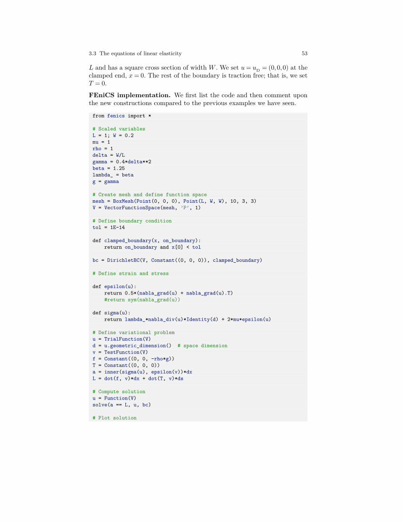
3.3 The equations of linear elasticity 53
L and has a square cross section of width W . We set u= uD = (0,0,0) at theclamped end, x= 0. The rest of the boundary is traction free; that is, we setT = 0.
FEniCS implementation. We first list the code and then comment uponthe new constructions compared to the previous examples we have seen.
from fenics import *
# Scaled variablesL = 1; W = 0.2mu = 1rho = 1delta = W/Lgamma = 0.4*delta**2beta = 1.25lambda_ = betag = gamma
# Create mesh and define function spacemesh = BoxMesh(Point(0, 0, 0), Point(L, W, W), 10, 3, 3)V = VectorFunctionSpace(mesh, ’P’, 1)
# Define boundary conditiontol = 1E-14
def clamped_boundary(x, on_boundary):return on_boundary and x[0] < tol
bc = DirichletBC(V, Constant((0, 0, 0)), clamped_boundary)
# Define strain and stress
def epsilon(u):return 0.5*(nabla_grad(u) + nabla_grad(u).T)#return sym(nabla_grad(u))
def sigma(u):return lambda_*nabla_div(u)*Identity(d) + 2*mu*epsilon(u)
# Define variational problemu = TrialFunction(V)d = u.geometric_dimension() # space dimensionv = TestFunction(V)f = Constant((0, 0, -rho*g))T = Constant((0, 0, 0))a = inner(sigma(u), epsilon(v))*dxL = dot(f, v)*dx + dot(T, v)*ds
# Compute solutionu = Function(V)solve(a == L, u, bc)
# Plot solution
54 3 A Gallery of finite element solvers
plot(u, title=’Displacement’, mode=’displacement’)
# Plot stresss = sigma(u) - (1./3)*tr(sigma(u))*Identity(d) # deviatoric stressvon_Mises = sqrt(3./2*inner(s, s))V = FunctionSpace(mesh, ’P’, 1)von_Mises = project(von_Mises, V)plot(von_Mises, title=’Stress intensity’)
# Compute magnitude of displacementu_magnitude = sqrt(dot(u, u))u_magnitude = project(u_magnitude, V)plot(u_magnitude, ’Displacement magnitude’)print(’min/max u:’,
u_magnitude.vector().array().min(),u_magnitude.vector().array().max())
This example program can be found in the file ft06_elasticity.py.
Vector function spaces. The primary unknown is now a vector field u andnot a scalar field, so we need to work with a vector function space:
V = VectorFunctionSpace(mesh, ’P’, 1)
With u = Function(V) we get u as a vector-valued finite element functionwith three components for this 3D problem.
Constant vectors. For the boundary condition u = (0,0,0), we must seta vector value to zero, not just a scalar. Such a vector constant is specifiedas Constant((0, 0, 0)) in FEniCS. The corresponding 2D code would useConstant((0, 0)). Later in the code, we also need f as a vector and specifyit as Constant((0, 0, rho*g)).
nabla_grad. The gradient and divergence operators now have a prefixnabla_. This is strictly not necessary in the present problem, but recom-mended in general for vector PDEs arising from continuum mechanics, if youinterpret ∇ as a vector in the PDE notation; see the box about nabla_gradin Section 3.4.2.
Stress computation. As soon as the displacement u is computed, we cancompute various stress measures. We will compute the von Mises stress de-fined as σM =
√32s : s where s is the deviatoric stress tensor
s= σ− 13tr(σ)I .
There is a one-to-one mapping between these formulas and the FEniCS code:
s = sigma(u) - (1./3)*tr(sigma(u))*Identity(d)von_Mises = sqrt(3./2*inner(s, s))
The von_Mises variable is now an expression that must be projected to afinite element space before we can visualize it:
3.3 The equations of linear elasticity 55
V = FunctionSpace(mesh, ’P’, 1)von_Mises = project(von_Mises, V)plot(von_Mises, title=’Stress intensity’)
Scaling. It is often advantageous to scale a problem as it reduces the needfor setting physical parameters, and one obtains dimensionsless numbers thatreflect the competition of parameters and physical effects. We develop thecode for the original model with dimensions, and run the scaled problemby tweaking parameters appropriately. Scaling reduces the number of activeparameters from 6 to 2 for the present application.
In Navier’s equation for u, arising from inserting (3.21) and (3.22) into(3.20),
−(λ+µ)∇(∇·u)−µ∇2u= f,
we insert coordinates made dimensionless by L, and u= u/U , which resultsin the dimensionless governing equation
−β∇(∇ · u)−∇2u= f , f = (0,0,γ),
where β = 1 +λ/µ is a dimensionless elasticity parameter and where
γ = %gL2
µU
is a dimensionless variable reflecting the ratio of the load %g and the shearstress term µ∇2u∼ µU/L2 in the PDE.
One option for the scaling is to chose U such that γ is of unit size(U = %gL2/µ). However, in elasticity, this leads to displacements of the sizeof the geometry, which makes plots look very strange. We therefore want thecharacteristic displacement to be a small fraction of the characteristic lengthof the geometry. This can be achieved by choosing U equal to the maxi-mum deflection of a clamped beam, for which there actually exists a formula:U = 3
2%gL2δ2/E, where δ = L/W is a parameter reflecting how slender the
beam is, and E is the modulus of elasticity. Thus, the dimensionless param-eter δ is very important in the problem (as expected, since δ 1 is whatgives beam theory!). Taking E to be of the same order as µ, which is the casefor many materials, we realize that γ ∼ δ−2 is an appropriate choice. Exper-imenting with the code to find a displacement that “looks right” in plots ofthe deformed geometry, points to γ = 0.4δ−2 as our final choice of γ.
The simulation code implements the problem with dimensions and physicalparameters λ, µ, %, g, L, and W . However, we can easily reuse this code fora scaled problem: just set µ= %= L= 1, W as W/L (δ−1), g = γ, and λ= β.
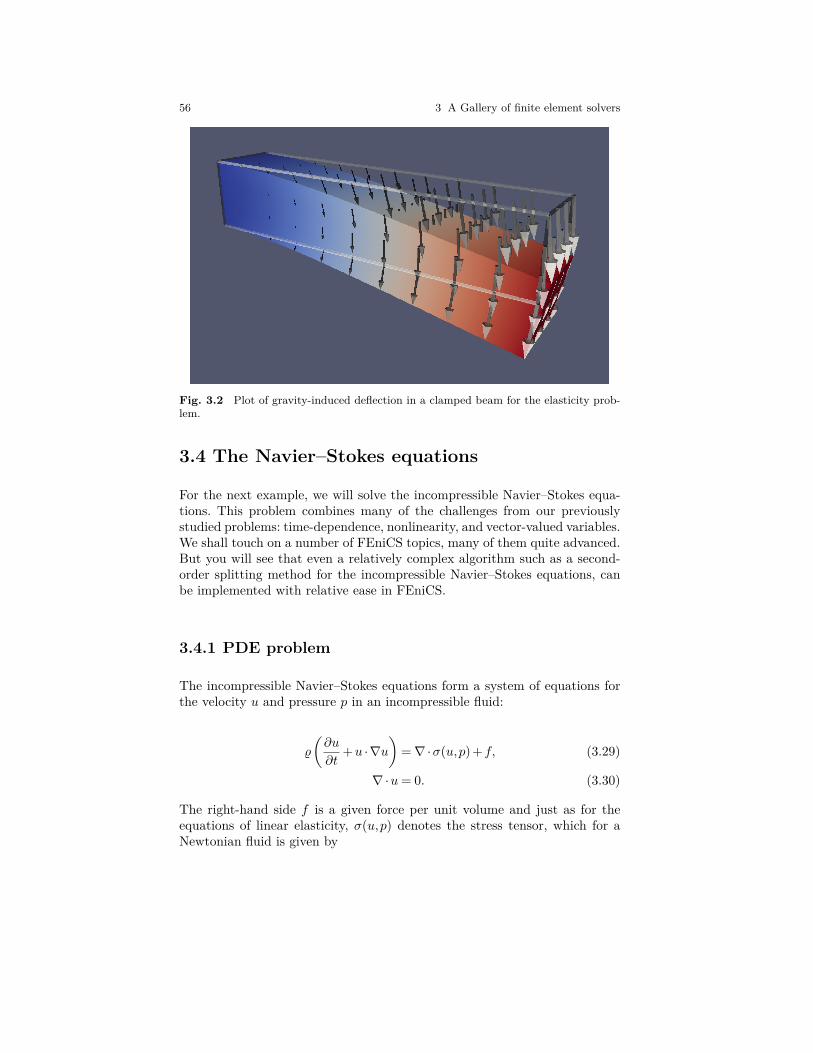
56 3 A Gallery of finite element solvers
Fig. 3.2 Plot of gravity-induced deflection in a clamped beam for the elasticity prob-lem.
3.4 The Navier–Stokes equations
For the next example, we will solve the incompressible Navier–Stokes equa-tions. This problem combines many of the challenges from our previouslystudied problems: time-dependence, nonlinearity, and vector-valued variables.We shall touch on a number of FEniCS topics, many of them quite advanced.But you will see that even a relatively complex algorithm such as a second-order splitting method for the incompressible Navier–Stokes equations, canbe implemented with relative ease in FEniCS.
3.4.1 PDE problem
The incompressible Navier–Stokes equations form a system of equations forthe velocity u and pressure p in an incompressible fluid:
%
(∂u
∂t+u ·∇u
)=∇·σ(u,p) +f, (3.29)
∇·u= 0. (3.30)
The right-hand side f is a given force per unit volume and just as for theequations of linear elasticity, σ(u,p) denotes the stress tensor, which for aNewtonian fluid is given by

3.4 The Navier–Stokes equations 57
σ(u,p) = 2µε(u)−pI, (3.31)
where ε(u) is the strain-rate tensor
ε(u) = 12
(∇u+ (∇u)T
).
The parameter µ is the dynamic viscosity. Note that the momentum equation(3.29) is very similar to the elasticity equation (3.20). The difference is in thetwo additional terms %(∂u/∂t+u ·∇u) and the different expression for thestress tensor. The two extra terms express the acceleration balanced by theforce F =∇·σ+f per unit volume in Newton’s second law of motion.
3.4.2 Variational formulation
The Navier–Stokes equations are different from the time-dependent heatequation in that we need to solve a system of equations and this systemis of a special type. If we apply the same technique as for the heat equa-tion; that is, replacing the time derivative with a simple difference quotient,we obtain a nonlinear system of equations. This in itself is not a problemfor FEniCS as we saw in Section 3.2, but the system has a so-called saddlepoint structure and requires special techniques (special preconditioners anditerative methods) to be solved efficiently.
Instead, we will apply a simpler and often very efficient approach, knownas a splitting method. The idea is to consider the two equations (3.29) and(3.30) separately. There exist many splitting strategies for the incompress-ible Navier–Stokes equations. One of the oldest is the method proposed byChorin [6] and Temam [31], often referred to as Chorin’s method. We willuse a modified version of Chorin’s method, the so-called incremental pres-sure correction scheme (IPCS) due to [13] which gives improved accuracycompared to the original scheme at little extra cost.
The IPCS scheme involves three steps. First, we compute a tentative ve-locity u? by advancing the momentum equation (3.29) by a midpoint finitedifference scheme in time, but using the pressure pn from the previous timeinterval. We will also linearize the nonlinear convective term by using theknown velocity un from the previous time step: un · ∇un. The variationalproblem for this first step is
〈%(u?−un)/∆t,v〉+ 〈%un ·∇un,v〉+ 〈σ(un+ 12 ,pn), ε(v)〉
+ 〈pnn,v〉∂Ω−〈µ∇un+ 12 ·n,v〉∂Ω = 〈fn+1,v〉. (3.32)
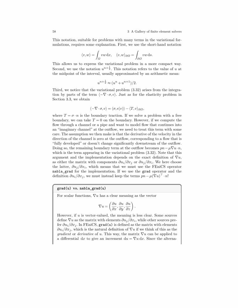
58 3 A Gallery of finite element solvers
This notation, suitable for problems with many terms in the variational for-mulations, requires some explanation. First, we use the short-hand notation
〈v,w〉=∫Ωvwdx, 〈v,w〉∂Ω =
∫∂Ω
vwds.
This allows us to express the variational problem in a more compact way.Second, we use the notation un+ 1
2 . This notation refers to the value of u atthe midpoint of the interval, usually approximated by an arithmetic mean:
un+ 12 ≈ (un+un+1)/2.
Third, we notice that the variational problem (3.32) arises from the integra-tion by parts of the term 〈−∇ · σ,v〉. Just as for the elasticity problem inSection 3.3, we obtain
〈−∇·σ,v〉= 〈σ,ε(v)〉−〈T,v〉∂Ω ,
where T = σ ·n is the boundary traction. If we solve a problem with a freeboundary, we can take T = 0 on the boundary. However, if we compute theflow through a channel or a pipe and want to model flow that continues intoan “imaginary channel” at the outflow, we need to treat this term with somecare. The assumption we then make is that the derivative of the velocity in thedirection of the channel is zero at the outflow, corresponding to a flow that is“fully developed” or doesn’t change significantly downstream of the outflow.Doing so, the remaining boundary term at the outflow becomes pn−µ∇u ·n,which is the term appearing in the variational problem (3.32). Note that thisargument and the implementation depends on the exact definition of ∇u,as either the matrix with components ∂ui/∂xj or ∂uj/∂xi. We here choosethe latter, ∂uj/∂xi, which means that we must use the FEniCS operatornabla_grad for the implementation. If we use the grad operator and thedefinition ∂ui/∂xj , we must instead keep the terms pn−µ(∇u)> ·n!
grad(u) vs. nabla_grad(u)
For scalar functions, ∇u has a clear meaning as the vector
∇u=(∂u
∂x,∂u
∂y,∂u
∂z
).
However, if u is vector-valued, the meaning is less clear. Some sourcesdefine∇u as the matrix with elements ∂uj/∂xi, while other sources pre-fer ∂ui/∂xj . In FEniCS, grad(u) is defined as the matrix with elements∂ui/∂xj , which is the natural definition of ∇u if we think of this as thegradient or derivative of u. This way, the matrix ∇u can be applied toa differential dx to give an increment du = ∇u dx. Since the alterna-

3.4 The Navier–Stokes equations 59
tive interpretation of ∇u as the matrix with elements ∂uj/∂xi is verycommon, in particular in continuum mechanics, FEniCS provides theoperator nabla_grad for this purpose. For the Navier–Stokes equations,it is important to consider the term u ·∇u which should be interpretedas the vector w with elements wi =
∑j
(uj
∂∂xj
)ui =
∑j uj
∂ui∂xj
. Thisterm can be implemented in FEniCS either as grad(u)*u, since thisis expression becomes
∑j ∂ui/∂xjuj , or as dot(u, nabla_grad(u))
since this expression becomes∑iui∂uj/∂xi. We will use the notation
dot(u, nabla_grad(u)) below since it corresponds more closely to thestandard notation u ·∇u.
To be more precise, there are three different notations used for PDEsinvolving gradient, divergence, and curl operators. One employs gradu,divu, and curlu operators. Another employs ∇u as a synonym forgradu, ∇·u means divu, and ∇×u is the name for curlu. The thirdoperates with ∇u, ∇ ·u, and ∇×u in which ∇ is a vector and, e.g.,∇u is a dyadic expression: (∇u)i,j = ∂uj/∂xi = (gradu)>. The latternotation, with ∇ as a vector operator, is often handy when derivingequations in continuum mechanics, and if this interpretation of ∇ is thefoundation of your PDE, you must use nabla_grad, nabla_div, andnabla_curl in FEniCS code as these operators are compatible withdyadic computations. From the Navier–Stokes equations we can easilysee what ∇ means: if the convective term has the form u ·∇u, actuallymeaning (u ·∇)u, then ∇ is a vector and the implementation becomesdot(u, nabla_grad(u)) in FEniCS, but if we see ∇u ·u or (gradu) ·u,the corresponding FEniCS expression is dot(grad(u), u).
Similarly, the divergence of a tensor field like the stress tensor σcan also be expressed in two different ways, as either div(sigma)or nabla_div(sigma). The first case corresponds to the components∂σij/∂xj and the second to ∂σij/∂xi. In general, these expressions willbe different but when the stress measure is symmetric, the expressionshave the same value.
We now move on to the second step in our splitting scheme for the in-compressible Navier–Stokes equations. In the first step, we computed thetentative velocity u? based on the pressure from the previous time step. Wemay now use the computed tentative velocity to compute the new pressurepn:
〈∇pn+1,∇q〉= 〈∇pn,∇q〉−∆t−1〈∇ ·u?, q〉. (3.33)
Note here that q is a scalar-valued test function from the pressure space,whereas the test function v in (3.32) is a vector-valued test function from thevelocity space.
One way to think about this step is to subtract the Navier–Stokes momen-tum equation (3.29) expressed in terms of the tentative velocity u? and the
60 3 A Gallery of finite element solvers
pressure pn from the momentum equation expressed in terms of the velocityun+1 and pressure pn+1. This results in the equation
(un+1−u?)/∆t+∇pn+1−∇pn = 0. (3.34)
Taking the divergence and requiring that ∇·un+1 = 0 by the Navier–Stokescontinuity equation (3.30), we obtain the equation −∇ ·u?/∆t+∇2pn+1−∇2pn = 0, which is a Poisson problem for the pressure pn+1 resulting in thevariational problem (3.33).
Finally, we compute the corrected velocity un+1 from the equation (3.34).Multiplying this equation by a test function v, we obtain
〈un+1,v〉= 〈u?,v〉−∆t〈∇(pn+1−pn),v〉. (3.35)
In summary, we may thus solve the incompressible Navier–Stokes equa-tions efficiently by solving a sequence of three linear variational problems ineach time step.
3.4.3 FEniCS implementation
Test problem 1: Channel flow. As a first test problem, we compute theflow between two infinite plates, so-called channel or Poiseuille flow. As weshall see, this problem has a known analytical solution. Let H be the distancebetween the plates and L the length of the channel. There are no body forces.
We may scale the problem first to get rid of seemingly independent physicalparameters. The physics of this problem is governed by viscous effects only,in the direction perpendicular to the flow, so a time scale should be based ondiffusion accross the channel: tc =H2/ν. We let U , some characteristic inflowvelocity, be the velocity scale and H the spatial scale. The pressure scale istaken as the characteristic shear stress, µU/H, since this is a primary exampleof shear flow. Inserting x= x/H, y = y/H, z = z/H, u= u/U , p=Hp/(µU),and t=H2/ν in the equations results in the scaled Navier–Stokes equations(dropping bars after the scaling):
∂u
∂t+ Reu ·∇u=−∇p+∇2u,
∇·u= 0 .
Here, Re = %UH/µ is the Reynolds number. Because of the time and pressurescales, which are different from convection-dominated fluid flow, the Reynoldsnumber is associated with the convective term and not the viscosity term.
The exact solution is derived by assuming u = (ux(x,y,z),0,0), with thex axis pointing along the channel. Since ∇ ·u = 0, u cannot depend on x.

3.4 The Navier–Stokes equations 61
The physics of channel flow is also two-dimensional so we can omit the zcoordinate (more precisely: ∂/∂z = 0). Inserting u= (ux,0,0) in the (scaled)governing equations gives u′′x(y) = ∂p/∂x. Differentiating this equation withrespect to x shows that ∂2p/∂2x= 0 so ∂p/∂x is a constant, here called −β.This is the driving force of the flow and can be specified as a known parameterin the problem. Integrating u′′x(y) =−β over the width of the channel, [0,1],and requiring u = (0,0,0) at the channel walls, results in ux = 1
2βy(1− y).The characteristic inlet velocity U can be taken as the maximum inflow aty= 1/2, implying β = 8. The length of the channel, L/H in the scaled model,has no impact on the result, so for simplicity we just compute on the unitsquare. Mathematically, the pressure must be prescribed at a point, but sincep does not depend on y, we can set p to a known value, e.g. zero, along theoutlet boundary x= 1. The result is p(x) = 8(1−x) and ux = 4y(1−y).
The boundary conditions can be set as p = 8 at x = 0, p = 0 at x = 1and u = (0,0,0) on the walls y = 0,1. This defines the pressure drop andshould result in unit maximum velocity at the inlet and outlet and a parabolicvelocity profile without further specifications. Note that it is only meaningfulto solve the Navier–Stokes equations in 2D or 3D geometries, although theunderlying mathematical problem collapses to two 1D problems, one for ux(y)and one for p(x).
The scaled model is not so easy to simulate using a standard Navier–Stokessolver with dimensions. However, one can argue that the convection term iszero, so the Re coefficient in front of this term in the scaled PDEs is notimportant and can be set to unity. In that case, setting % = µ = 1 in theoriginal Navier–Stokes equations resembles the scaled model.
For a specific engineering problem one wants to simulate a specific fluidand set corresponding parameters. A general solver is therefore most naturallyimplemented with dimensions and the original physical parameters. However,scaling may greatly simplify numerical simulations. First of all, it shows thatall fluids behave in the same way: it does not matter whether we have oil,gas, or water flowing between two plates, and it does not matter how fastthe flow is (up to some criticial value of the Reynolds number where theflow becomes unstable and transitions to a complicated turbulent flow oftotally different nature). This means that one simulation is enough to coverall types of channel flow! In other applications, scaling shows that it might benecessary to set just the fraction of some parameters (dimensionless numbers)rather than the parameters themselves. This simplifies exploring the inputparameter space which is often the purpose of simulation. Frequently, thescaled problem is run by setting some of the input parameters with dimensionto fixed values (often unity).
FEniCS implementation. Our previous examples have all started out withthe creation of a mesh and then the definition of a FunctionSpace on themesh. For the Navier–Stokes splitting scheme we will need to define twofunction spaces, one for the velocity and one for the pressure:

62 3 A Gallery of finite element solvers
V = VectorFunctionSpace(mesh, ’P’, 2)Q = FunctionSpace(mesh, ’P’, 1)
The first space V is a vector-valued function space for the velocity and thesecond space Q is a scalar-valued function space for the pressure. We usepiecewise quadratic elements for the velocity and piecewise linear elementsfor the pressure. When creating a VectorFunctionSpace in FEniCS, thevalue-dimension (the length of the vectors) will be set equal to the geometricdimension of the finite element mesh. One can easily create vector-valuedfunction spaces with other dimensions in FEniCS by adding the keywordparameter dim:
V = VectorFunctionSpace(mesh, ’P’, 2, dim=10)
Stable finite element spaces for the Navier–Stokes equations
It is well-known that certain finite element spaces are not stable for theNavier–Stokes equations, or even for the simpler Stokes equations. Theprime example of an unstable pair of finite element spaces is to use firstdegree continuous piecewise polynomials for both the velocity and thepressure. Using an unstable pair of spaces typically results in a solu-tion with spurious (unwanted, non-physical) oscillations in the pressuresolution. The simple remedy is to use continuous piecewise quadraticelements for the velocity and continuous piecewise linear elements forthe pressure. Together, these elements form the so-called Taylor-Hoodelement. Spurious oscillations may occur also for splitting methods ifan unstable element pair is used.
Since we have two different function spaces, we need to create two sets oftrial and test functions:
u = TrialFunction(V)v = TestFunction(V)p = TrialFunction(Q)q = TestFunction(Q)
As we have seen in previous examples, boundaries may be defined in FEn-iCS by defining Python functions that return True or False depending onwhether a point should be considered part of the boundary, for example
def boundary(x, on_boundary):return near(x[0], 0)
This function defines the boundary to be all points with x-coordinateequal to (near) zero. The near function comes from FEniCS and per-forms a test with tolerance: abs(x[0] - 0) < 3E-16 so we do not run intorounding troubles. Alternatively, we may give the boundary definition as a

3.4 The Navier–Stokes equations 63
string of C++ code, much like we have previously defined expressions suchas u_D = Expression(’1 + x[0]*x[0] + 2*x[1]*x[1]’, degree=2). Theabove definition of the boundary in terms of a Python function may thus bereplaced by a simple C++ string:
boundary = ’near(x[0], 0)’
This has the advantage of moving the computation of which nodes belongto the boundary from Python to C++, which improves the efficiency of theprogram.
For the current example, we will set three different boundary conditions.First, we will set u= 0 at the walls of the channel; that is, at y = 0 and y = 1.Second, we will set p= 8 at the inflow (x= 0) and, finally, p= 0 at the outflow(x = 1). This will result in a pressure gradient that will accelerate the flowfrom the initial state with zero velocity. These boundary conditions may bedefined as follows:
# Define boundariesinflow = ’near(x[0], 0)’outflow = ’near(x[0], 1)’walls = ’near(x[1], 0) || near(x[1], 1)’
# Define boundary conditionsbcu_noslip = DirichletBC(V, Constant((0, 0)), walls)bcp_inflow = DirichletBC(Q, Constant(8), inflow)bcp_outflow = DirichletBC(Q, Constant(0), outflow)bcu = [bcu_noslip]bcp = [bcp_inflow, bcp_outflow]
At the end, we collect the boundary conditions for the velocity and pressurein Python lists so we can easily access them in the following computation.
We now move on to the definition of the variational forms. There are threevariational problems to be defined, one for each step in the IPCS scheme. Letus look at the definition of the first variational problem. We start with someconstants:
U = 0.5*(u_n + u)n = FacetNormal(mesh)f = Constant((0, 0))k = Constant(dt)mu = Constant(mu)rho = Constant(rho)
The next step is to set up the variational form for the first step (3.32) inthe solution process. Since the variational problem contains a mix of knownand unknown quantities we will use the following naming convention: u isthe unknown (mathematically un+1) as a trial function in the variationalform, u_ is the most recently computed approximation (un+1 available as aFunction object), u_n is un, and the same convention goes for p, p_ (pn+1),and p_n (pn).

64 3 A Gallery of finite element solvers
# Define strain-rate tensordef epsilon(u):
return sym(nabla_grad(u))
# Define stress tensordef sigma(u, p):
return 2*mu*epsilon(u) - p*Identity(len(u))
# Define variational problem for step 1F1 = rho*dot((u - u_n) / k, v)*dx + \
rho*dot(dot(u_n, nabla_grad(u_n)), v)*dx \+ inner(sigma(U, p_n), epsilon(v))*dx \+ dot(p_n*n, v)*ds - dot(mu*nabla_grad(U)*n, v)*ds \- dot(f, v)*dx
a1 = lhs(F1)L1 = rhs(F1)
Note that we take advantage of the Python programming language todefine our own operators sigma and epsilon. Using Python this way makesit easy to extend the mathematical language of FEniCS with special operatorsand constitutive laws.
Also note that FEniCS can sort out the bilinear form a(u,v) and linearform L(v) forms by the lhs and rhs functions. This is particularly convenientin longer and more complicated variational forms.
The splitting scheme requires the solution of a sequence of three variationalproblems in each time step. We have previously used the built-in FEniCSfunction solve to solve variational problems. Under the hood, when a usercalls solve(a == L, u, bc), FEniCS will perform the following steps:
A = assemble(A)b = assemble(L)bc.apply(A, b)solve(A, u.vector(), b)
In the last step, FEniCS uses the overloaded solve function to solve thelinear system AU = b where U is the vector of degrees of freedom for thefunction u(x) =
∑j=1Ujφj(x).
In our implementation of the splitting scheme, we will make use of theselow-level commands to first assemble and then call solve. This has the ad-vantage that we may control when we assemble and when we solve the linearsystem. In particular, since the matrices for the three variational problemsare all time-independent, it makes sense to assemble them once and for alloutside of the time-stepping loop:
A1 = assemble(a1)A2 = assemble(a2)A3 = assemble(a3)
Within the time-stepping loop, we may then assemble only the right-handside vectors, apply boundary conditions, and call the solve function as herefor the first of the three steps:
3.4 The Navier–Stokes equations 65
# Time-steppingt = 0for n in range(num_steps):
# Update current timet += dt
# Step 1: Tentative velocity stepb1 = assemble(L1)[bc.apply(b1) for bc in bcu]solve(A1, u_.vector(), b1)
Notice the Python list comprehension [bc.apply(b1) for bc in bcu] whichiterates over all bc in the list bcu. This is a convenient and compact way toconstruct a loop that applies all boundary conditions in a single line. Also,the code works if we add more Dirichlet boundary conditions in the future.Note that the boundary conditions only need to be applied to the right-handside vectors as they have already been applied to the matrices (not shown).
Finally, let us look at an important detail in how we use parameters suchas the time step dt in the definition of our variational problems. Since wemight want to change these later, for example if we want to experiment withsmaller or larger time steps, we wrap these using a FEniCS Constant:
k = Constant(dt)
The assembly of matrices and vectors in FEniCS is based on code genera-tion. This means that whenever we change a variational problem, FEniCS willhave to generate new code, which may take a little time. New code will alsobe generated and compiled when a float value for the time step is changed. Bywrapping this parameter using Constant, FEniCS will treat the parameteras a generic constant and not as a specific numerical value, which preventsrepeated code generation. In the case of the time step, we choose a new namek instead of dt for the Constant since we also want to use the variable dt asa Python float as part of the time-stepping.
The complete code for simulating 2D channel flow with FEniCS can befound in the file ft07_navier_stokes_channel.py.Verification. We compute the error at the nodes as we have done before toverify that our implementation is correct. Our Navier–Stokes solver computesthe solution to the time-dependent incompressible Navier–Stokes equations,starting from the initial condition u= (0,0). We have not specified the initialcondition explicitly in our solver which means that FEniCS will initialize allvariables, in particular the previous and current velocities u_n and u_, tozero. Since the exact solution is quadratic, we expect the solution to be exactto within machine precision at the nodes at infinite time. For our implemen-tation, the error quickly approaches zero and is approximately 10−6 at timeT = 10.Test problem 2: Flow past a cylinder. We now turn our attention to amore challenging problem: flow past a circular cylinder. The geometry and pa-
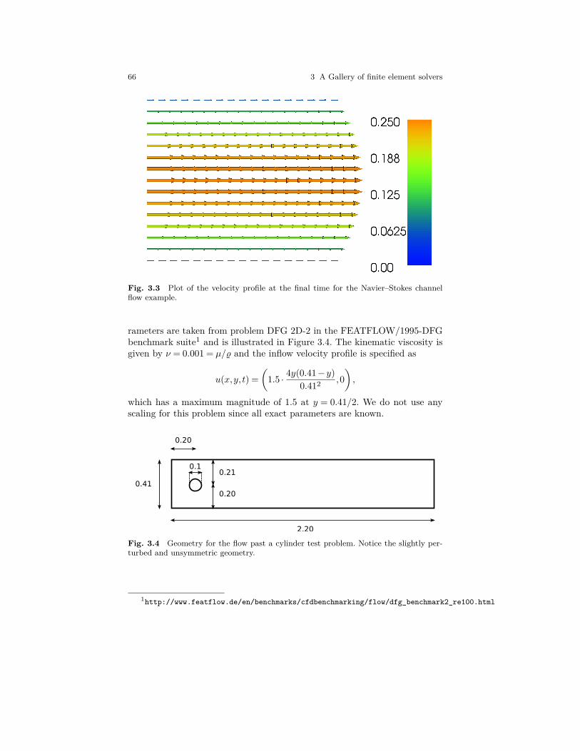
66 3 A Gallery of finite element solvers
Fig. 3.3 Plot of the velocity profile at the final time for the Navier–Stokes channelflow example.
rameters are taken from problem DFG 2D-2 in the FEATFLOW/1995-DFGbenchmark suite1 and is illustrated in Figure 3.4. The kinematic viscosity isgiven by ν = 0.001 = µ/% and the inflow velocity profile is specified as
u(x,y, t) =(
1.5 · 4y(0.41−y)0.412 ,0
),
which has a maximum magnitude of 1.5 at y = 0.41/2. We do not use anyscaling for this problem since all exact parameters are known.
0.21
0.20
0.20
0.41
2.20
0.1
Fig. 3.4 Geometry for the flow past a cylinder test problem. Notice the slightly per-turbed and unsymmetric geometry.
1http://www.featflow.de/en/benchmarks/cfdbenchmarking/flow/dfg_benchmark2_re100.html
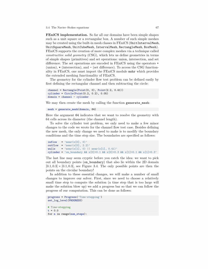
3.4 The Navier–Stokes equations 67
FEniCS implementation. So far all our domains have been simple shapessuch as a unit square or a rectangular box. A number of such simple meshesmay be created using the built-in mesh classes in FEniCS (UnitIntervalMesh,UnitSquareMesh, UnitCubeMesh, IntervalMesh, RectangleMesh, BoxMesh).FEniCS supports the creation of more complex meshes via a technique calledconstructive solid geometry (CSG), which lets us define geometries in termsof simple shapes (primitives) and set operations: union, intersection, and setdifference. The set operations are encoded in FEniCS using the operators +(union), * (intersection), and - (set difference). To access the CSG function-ality in FEniCS, one must import the FEniCS module mshr which providesthe extended meshing functionality of FEniCS.
The geometry for the cylinder flow test problem can be defined easily byfirst defining the rectangular channel and then subtracting the circle:
channel = Rectangle(Point(0, 0), Point(2.2, 0.41))cylinder = Circle(Point(0.2, 0.2), 0.05)domain = channel - cylinder
We may then create the mesh by calling the function generate_mesh:
mesh = generate_mesh(domain, 64)
Here the argument 64 indicates that we want to resolve the geometry with64 cells across its diameter (the channel length).
To solve the cylinder test problem, we only need to make a few minorchanges to the code we wrote for the channel flow test case. Besides definingthe new mesh, the only change we need to make is to modify the boundaryconditions and the time step size. The boundaries are specified as follows:
inflow = ’near(x[0], 0)’outflow = ’near(x[0], 2.2)’walls = ’near(x[1], 0) || near(x[1], 0.41)’cylinder = ’on_boundary && x[0]>0.1 && x[0]<0.3 && x[1]>0.1 && x[1]<0.3’
The last line may seem cryptic before you catch the idea: we want to pickout all boundary points (on_boundary) that also lie within the 2D domain[0.1,0.3]× [0.1,0.3], see Figure 3.4. The only possible points are then thepoints on the circular boundary!
In addition to these essential changes, we will make a number of smallchanges to improve our solver. First, since we need to choose a relativelysmall time step to compute the solution (a time step that is too large willmake the solution blow up) we add a progress bar so that we can follow theprogress of our computation. This can be done as follows:
progress = Progress(’Time-stepping’)set_log_level(PROGRESS)
# Time-steppingt = 0.0for n in range(num_steps):
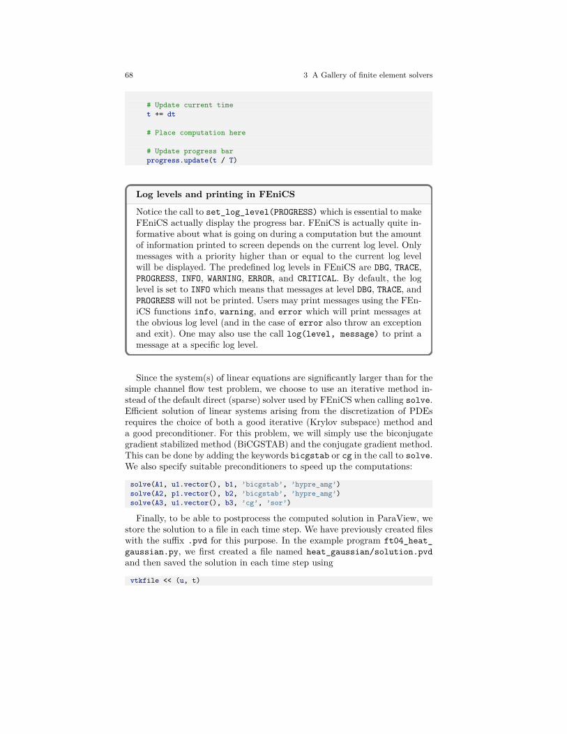
68 3 A Gallery of finite element solvers
# Update current timet += dt
# Place computation here
# Update progress barprogress.update(t / T)
Log levels and printing in FEniCS
Notice the call to set_log_level(PROGRESS) which is essential to makeFEniCS actually display the progress bar. FEniCS is actually quite in-formative about what is going on during a computation but the amountof information printed to screen depends on the current log level. Onlymessages with a priority higher than or equal to the current log levelwill be displayed. The predefined log levels in FEniCS are DBG, TRACE,PROGRESS, INFO, WARNING, ERROR, and CRITICAL. By default, the loglevel is set to INFO which means that messages at level DBG, TRACE, andPROGRESS will not be printed. Users may print messages using the FEn-iCS functions info, warning, and error which will print messages atthe obvious log level (and in the case of error also throw an exceptionand exit). One may also use the call log(level, message) to print amessage at a specific log level.
Since the system(s) of linear equations are significantly larger than for thesimple channel flow test problem, we choose to use an iterative method in-stead of the default direct (sparse) solver used by FEniCS when calling solve.Efficient solution of linear systems arising from the discretization of PDEsrequires the choice of both a good iterative (Krylov subspace) method anda good preconditioner. For this problem, we will simply use the biconjugategradient stabilized method (BiCGSTAB) and the conjugate gradient method.This can be done by adding the keywords bicgstab or cg in the call to solve.We also specify suitable preconditioners to speed up the computations:
solve(A1, u1.vector(), b1, ’bicgstab’, ’hypre_amg’)solve(A2, p1.vector(), b2, ’bicgstab’, ’hypre_amg’)solve(A3, u1.vector(), b3, ’cg’, ’sor’)
Finally, to be able to postprocess the computed solution in ParaView, westore the solution to a file in each time step. We have previously created fileswith the suffix .pvd for this purpose. In the example program ft04_heat_gaussian.py, we first created a file named heat_gaussian/solution.pvdand then saved the solution in each time step using
vtkfile << (u, t)

3.4 The Navier–Stokes equations 69
For the present example, we will instead choose to save the solution toXDMF format. This file format works similarly to the .pvd files we have seenearlier but has several advantages. First, the storage is much more efficient,both in terms of speed and file sizes. Second, .xdmf files work in parallell,both for writing and reading (postprocessing). Much like .pvd files, the actualdata will not be stored in the .xdmf file itself, but will instead be stored ina (single) separate data file with the suffix .hdf5 which is an advanced fileformat designed for high-performance computing. We create the XDMF filesas follows:
xdmffile_u = XDMFFile(’navier_stokes_cylinder/velocity.xdmf’)xdmffile_p = XDMFFile(’navier_stokes_cylinder/pressure.xdmf’)
In each time step, we may then store the velocity and pressure by
xdmffile_u.write(u, t)xdmffile_p.write(p, t)
We also store the solution using a FEniCS TimeSeries. This allows us tostore the solution not for visualization, but for later reuse in a computationas we will see in the next section. Using a TimeSeries it is easy and efficientto read in solutions from certain points in time during a simulation. TheTimeSeries class also uses the HDF5 file format for efficient storage andaccess to data.
Figures 3.5 and 3.6 show the velocity and pressure at final time visualizedin ParaView. For the visualization of the velocity, we have used the Glyphfilter to visualize the vector velocity field. For the visualization of the pressure,we have used the Warp By Scalar filter.
Fig. 3.5 Plot of the velocity for the cylinder test problem at final time.
The complete code for the cylinder test problem looks as follows:
from fenics import *from mshr import *import numpy as np
T = 5.0 # final timenum_steps = 5000 # number of time stepsdt = T / num_steps # time step sizemu = 0.001 # dynamic viscosity

70 3 A Gallery of finite element solvers
Fig. 3.6 Plot of the pressure for the cylinder test problem at final time.
rho = 1 # density
# Create meshchannel = Rectangle(Point(0, 0), Point(2.2, 0.41))cylinder = Circle(Point(0.2, 0.2), 0.05)domain = channel - cylindermesh = generate_mesh(domain, 64)
# Define function spacesV = VectorFunctionSpace(mesh, ’P’, 2)Q = FunctionSpace(mesh, ’P’, 1)
# Define boundariesinflow = ’near(x[0], 0)’outflow = ’near(x[0], 2.2)’walls = ’near(x[1], 0) || near(x[1], 0.41)’cylinder = ’on_boundary && x[0]>0.1 && x[0]<0.3 && x[1]>0.1 && x[1]<0.3’
# Define inflow profileinflow_profile = (’4.0*1.5*x[1]*(0.41 - x[1]) / pow(0.41, 2)’, ’0’)
# Define boundary conditionsbcu_inflow = DirichletBC(V, Expression(inflow_profile, degree=2), inflow)bcu_walls = DirichletBC(V, Constant((0, 0)), walls)bcu_cylinder = DirichletBC(V, Constant((0, 0)), cylinder)bcp_outflow = DirichletBC(Q, Constant(0), outflow)bcu = [bcu_inflow, bcu_walls, bcu_cylinder]
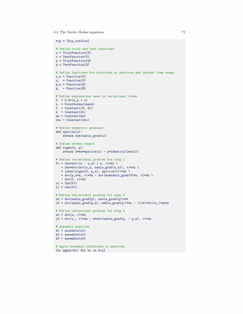
3.4 The Navier–Stokes equations 71
bcp = [bcp_outflow]
# Define trial and test functionsu = TrialFunction(V)v = TestFunction(V)p = TrialFunction(Q)q = TestFunction(Q)
# Define functions for solutions at previous and current time stepsu_n = Function(V)u_ = Function(V)p_n = Function(Q)p_ = Function(Q)
# Define expressions used in variational formsU = 0.5*(u_n + u)n = FacetNormal(mesh)f = Constant((0, 0))k = Constant(dt)mu = Constant(mu)rho = Constant(rho)
# Define symmetric gradientdef epsilon(u):
return sym(nabla_grad(u))
# Define stress tensordef sigma(u, p):
return 2*mu*epsilon(u) - p*Identity(len(u))
# Define variational problem for step 1F1 = rho*dot((u - u_n) / k, v)*dx \
+ rho*dot(dot(u_n, nabla_grad(u_n)), v)*dx \+ inner(sigma(U, p_n), epsilon(v))*dx \+ dot(p_n*n, v)*ds - dot(mu*nabla_grad(U)*n, v)*ds \- dot(f, v)*dx
a1 = lhs(F1)L1 = rhs(F1)
# Define variational problem for step 2a2 = dot(nabla_grad(p), nabla_grad(q))*dxL2 = dot(nabla_grad(p_n), nabla_grad(q))*dx - (1/k)*div(u_)*q*dx
# Define variational problem for step 3a3 = dot(u, v)*dxL3 = dot(u_, v)*dx - k*dot(nabla_grad(p_ - p_n), v)*dx
# Assemble matricesA1 = assemble(a1)A2 = assemble(a2)A3 = assemble(a3)
# Apply boundary conditions to matrices[bc.apply(A1) for bc in bcu]
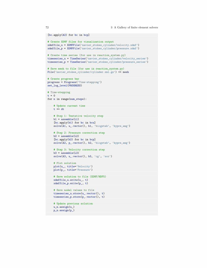
72 3 A Gallery of finite element solvers
[bc.apply(A2) for bc in bcp]
# Create XDMF files for visualization outputxdmffile_u = XDMFFile(’navier_stokes_cylinder/velocity.xdmf’)xdmffile_p = XDMFFile(’navier_stokes_cylinder/pressure.xdmf’)
# Create time series (for use in reaction_system.py)timeseries_u = TimeSeries(’navier_stokes_cylinder/velocity_series’)timeseries_p = TimeSeries(’navier_stokes_cylinder/pressure_series’)
# Save mesh to file (for use in reaction_system.py)File(’navier_stokes_cylinder/cylinder.xml.gz’) << mesh
# Create progress barprogress = Progress(’Time-stepping’)set_log_level(PROGRESS)
# Time-steppingt = 0for n in range(num_steps):
# Update current timet += dt
# Step 1: Tentative velocity stepb1 = assemble(L1)[bc.apply(b1) for bc in bcu]solve(A1, u_.vector(), b1, ’bicgstab’, ’hypre_amg’)
# Step 2: Pressure correction stepb2 = assemble(L2)[bc.apply(b2) for bc in bcp]solve(A2, p_.vector(), b2, ’bicgstab’, ’hypre_amg’)
# Step 3: Velocity correction stepb3 = assemble(L3)solve(A3, u_.vector(), b3, ’cg’, ’sor’)
# Plot solutionplot(u_, title=’Velocity’)plot(p_, title=’Pressure’)
# Save solution to file (XDMF/HDF5)xdmffile_u.write(u_, t)xdmffile_p.write(p_, t)
# Save nodal values to filetimeseries_u.store(u_.vector(), t)timeseries_p.store(p_.vector(), t)
# Update previous solutionu_n.assign(u_)p_n.assign(p_)

3.5 A system of advection–diffusion–reaction equations 73
# Update progress barprogress.update(t / T)print(’u max:’, u_.vector().array().max())
# Hold plotinteractive()
This program can be found in the file ft08_navier_stokes_cylinder.py.The reader should be advised that this example program is considerably moredemanding than our previous examples in terms of CPU time and memory,but it should be possible to run the program on a reasonably modern laptop.
3.5 A system of advection–diffusion–reactionequations
The problems we have encountered so far—with the notable exception of theNavier–Stokes equations—all share a common feature: they all involve mod-els expressed by a single scalar or vector PDE. In many situations the modelis instead expressed as a system of PDEs, describing different quantities pos-sibly governed by (very) different physics. As we saw for the Navier–Stokesequations, one way to solve a system of PDEs in FEniCS is to use a splittingmethod where we solve one equation at a time and feed the solution fromone equation into the next. However, one of the strengths with FEniCS isthe ease by which one can instead define variational problems that coupleseveral PDEs into one compound system. In this section, we will look at howto use FEniCS to write solvers for such systems of coupled PDEs. The goalis to demonstrate how easy it is to implement fully implicit, also known asmonolithic, solvers in FEniCS.
3.5.1 PDE problem
Our model problem is the following system of advection–diffusion–reactionequations:
∂u1∂t
+w ·∇u1−∇· (ε∇u1) = f1−Ku1u2, (3.36)
∂u2∂t
+w ·∇u2−∇· (ε∇u2) = f2−Ku1u2, (3.37)
∂u3∂t
+w ·∇u3−∇· (ε∇u3) = f3 +Ku1u2−Ku3. (3.38)
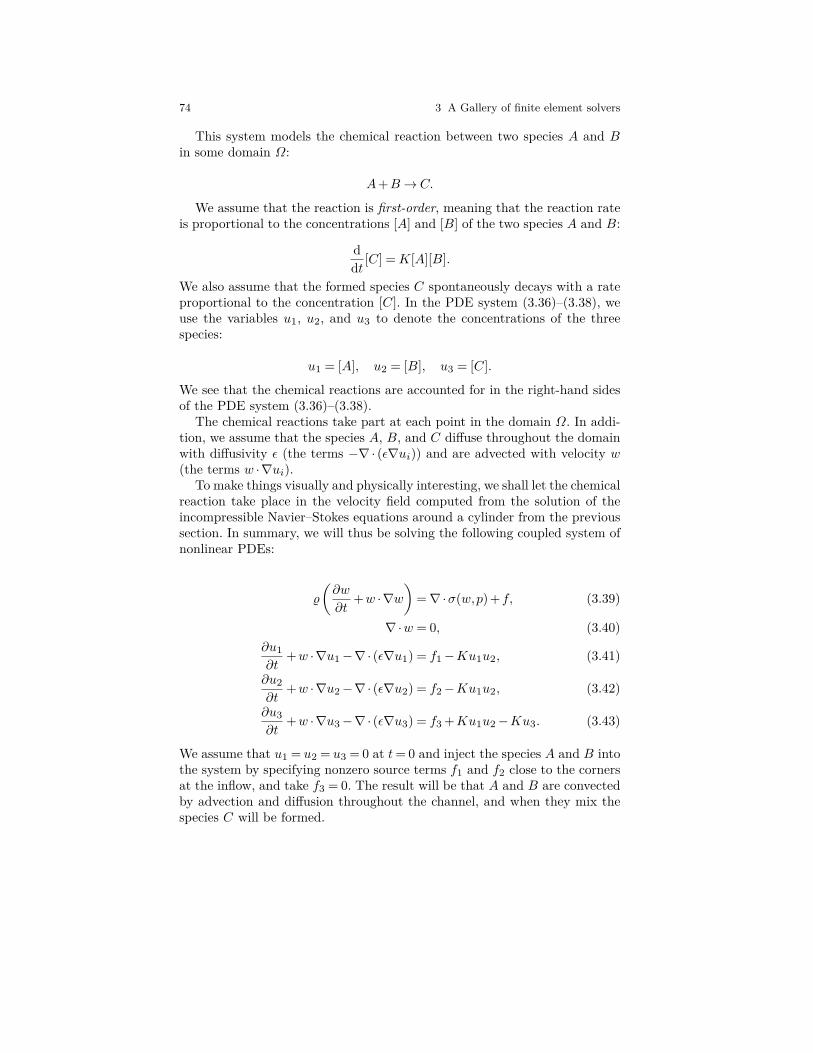
74 3 A Gallery of finite element solvers
This system models the chemical reaction between two species A and Bin some domain Ω:
A+B→ C.
We assume that the reaction is first-order, meaning that the reaction rateis proportional to the concentrations [A] and [B] of the two species A and B:
ddt [C] =K[A][B].
We also assume that the formed species C spontaneously decays with a rateproportional to the concentration [C]. In the PDE system (3.36)–(3.38), weuse the variables u1, u2, and u3 to denote the concentrations of the threespecies:
u1 = [A], u2 = [B], u3 = [C].
We see that the chemical reactions are accounted for in the right-hand sidesof the PDE system (3.36)–(3.38).
The chemical reactions take part at each point in the domain Ω. In addi-tion, we assume that the species A, B, and C diffuse throughout the domainwith diffusivity ε (the terms −∇· (ε∇ui)) and are advected with velocity w(the terms w ·∇ui).
To make things visually and physically interesting, we shall let the chemicalreaction take place in the velocity field computed from the solution of theincompressible Navier–Stokes equations around a cylinder from the previoussection. In summary, we will thus be solving the following coupled system ofnonlinear PDEs:
%
(∂w
∂t+w ·∇w
)=∇·σ(w,p) +f, (3.39)
∇·w = 0, (3.40)∂u1∂t
+w ·∇u1−∇· (ε∇u1) = f1−Ku1u2, (3.41)
∂u2∂t
+w ·∇u2−∇· (ε∇u2) = f2−Ku1u2, (3.42)
∂u3∂t
+w ·∇u3−∇· (ε∇u3) = f3 +Ku1u2−Ku3. (3.43)
We assume that u1 = u2 = u3 = 0 at t= 0 and inject the species A and B intothe system by specifying nonzero source terms f1 and f2 close to the cornersat the inflow, and take f3 = 0. The result will be that A and B are convectedby advection and diffusion throughout the channel, and when they mix thespecies C will be formed.

3.5 A system of advection–diffusion–reaction equations 75
Since the system is one-way coupled from the Navier–Stokes subsystem tothe advection–diffusion–reaction subsystem, we do not need to recompute thesolution to the Navier–Stokes equations, but can just read back the previouslycomputed velocity field w and feed it into our equations. But we do need tolearn how to read and write solutions for time-dependent PDE problems.
3.5.2 Variational formulation
We obtain the variational formulation of our system by multiplying eachequation by a test function, integrating the second-order terms −∇· (ε∇ui)by parts, and summing up the equations. When working with FEniCS it isconvenient to think of the PDE system as a vector of equations. The testfunctions are collected in a vector too, and the variational formulation is theinner product of the vector PDE and the vector test function.
We also need introduce some discretization in time. We will use the back-ward Euler method as before when we solved the heat equation and approx-imate the time derivatives by (un+1
i −uni )/∆t. Let v1, v2, and v3 be the testfunctions, or the components of the test vector function. The inner productresults in
∫Ω
(∆t−1(un+11 −un1 )v1 +w ·∇un+1
1 v1 + ε∇un+11 ·∇v1)dx (3.44)
+∫Ω
(∆t−1(un+12 −un2 )v2 +w ·∇un+1
2 v2 + ε∇un+12 ·∇v2)dx
+∫Ω
(∆t−1(un+13 −un3 )v3 +w ·∇un+1
3 v3 + ε∇un+13 ·∇v3)dx
−∫Ω
(f1v1 +f2v2 +f3v3)dx
−∫Ω
(−Kun+11 un+1
2 v1−Kun+11 un+1
2 v2 +Kun+11 un+1
2 v3−Kun+13 v3)dx= 0.
For this problem it is natural to assume homogeneous Neumann boundaryconditions on the entire boundary for u1, u2, and u3; that is, ∂ui/∂n= 0 fori= 1,2,3. This means that the boundary terms vanish when we integrate byparts.

76 3 A Gallery of finite element solvers
3.5.3 FEniCS implementation
The first step is to read the mesh from file. Luckily, we made sure to save themesh to file in the Navier–Stokes example and can now easily read it backfrom file:
mesh = Mesh(’navier_stokes_cylinder/cylinder.xml.gz’)
The mesh is stored in the native FEniCS XML format (with additional gzip-ping to decrease the file size).
Next, we need to define the finite element function space. For this problem,we need to define several spaces. The first space we create is the space forthe velocity field w from the Navier–Stokes simulation. We call this space Wand define the space by
W = VectorFunctionSpace(mesh, ’P’, 2)
It is important that this space is exactly the same as the space we used for thevelocity field in the Navier–Stokes solver. To read the values for the velocityfield, we use a TimeSeries:
timeseries_w = TimeSeries(’navier_stokes_cylinder/velocity_series’)
This will initialize the object timeseries_w which we will call later in thetime-stepping loop to retrieve values from the file velocity_series.h5 (inbinary HDF5 format).
For the three concentrations u1, u2, and u3, we want to create a mixedspace with functions that represent the full system (u1,u2,u3) as a singleentity. To do this, we need to define a MixedElement as the product space ofthree simple finite elements and then used the mixed element to define thefunction space:
P1 = FiniteElement(’P’, triangle, 1)element = MixedElement([P1, P1, P1])V = FunctionSpace(mesh, element)
Mixed elements as products of elements
FEniCS also allows finite elements to be defined as products of simpleelements (or mixed elements). For example, the well-known Taylor–Hood element, with quadratic velocity components and linear pressurefunctions, may be defined as follows:
P2 = VectorElement(’P’, triangle, 2)P1 = FiniteElement(’P’, triangle, 1)TH = P2 * P1

3.5 A system of advection–diffusion–reaction equations 77
This syntax works great for two elements, but for three or more ele-ments we meet a subtle issue in how the Python interpreter handles the* operator. For the reaction system, we create the mixed element byelement = MixedElement([P1, P1, P1]) and one would be temptedto write
element = P1 * P1 * P1
However, this is equivalent to writing element = (P1 * P1) * P1 sothe result will be a mixed element consisting of two subsystems, thefirst of which in turn consists of two scalar subsystems.
Finally, we remark that for the simple case of a mixed system con-sisting of three scalar elements as for the reaction system, the definitionis in fact equivalent to using a standard vector-valued element:
element = VectorElement(’P’, triangle, 1, dim=3)V = FunctionSpace(mesh, element)
Once the space has been created, we need to define our test functions andfinite element functions. Test functions for a mixed function space can becreated by replacing TestFunction by TestFunctions:
v_1, v_2, v_3 = TestFunctions(V)
Since the problem is nonlinear, we need to work with functions rather thantrial functions for the unknowns. This can be done by using the correspondingFunctions construction in FEniCS. However, as we will need to access theFunction for the entire system itself, we first need to create that functionand then access its components:
u = Function(V)u_1, u_2, u_3 = split(u)
These functions will be used to represent the unknowns u1, u2, and u3 at thenew time level n+ 1. The corresponding values at the previous time level nare denoted by u_n1, u_n2, and u_n3 in our program.
When now all functions and test functions have been defined, we canexpress the nonlinear variational problem (3.44):
F = ((u_1 - u_n1) / k)*v_1*dx + dot(w, grad(u_1))*v_1*dx \+ eps*dot(grad(u_1), grad(v_1))*dx + K*u_1*u_2*v_1*dx \+ ((u_2 - u_n2) / k)*v_2*dx + dot(w, grad(u_2))*v_2*dx \+ eps*dot(grad(u_2), grad(v_2))*dx + K*u_1*u_2*v_2*dx \+ ((u_3 - u_n3) / k)*v_3*dx + dot(w, grad(u_3))*v_3*dx \+ eps*dot(grad(u_3), grad(v_3))*dx - K*u_1*u_2*v_3*dx + K*u_3*v_3*dx \- f_1*v_1*dx - f_2*v_2*dx - f_3*v_3*dx
The time-stepping simply consists of solving this variational problem ineach time step by a call to the solve function:

78 3 A Gallery of finite element solvers
t = 0for n in range(num_steps):
t += dttimeseries_w.retrieve(w.vector(), t)solve(F == 0, u)u_n.assign(u)
In each time step, we first read the current value for the velocity field from thetime series we have previously stored. We then solve the nonlinear system,and assign the computed values to the left-hand side values for the nexttime interval. When retrieving values from a TimeSeries, the values will bydefault be interpolated (linearly) to the given time t if the time does notexactly match a sample in the series.
The solution at the final time is shown in Figure 3.7. We clearly see theadvection of the species A and B and the formation of C along the center ofthe channel where A and B meet.
Fig. 3.7 Plot of the concentrations of the three species A, B, and C (from top tobottom) at final time.
The complete code is presented below.
from fenics import *
T = 5.0 # final timenum_steps = 500 # number of time stepsdt = T / num_steps # time step sizeeps = 0.01 # diffusion coefficientK = 10.0 # reaction rate
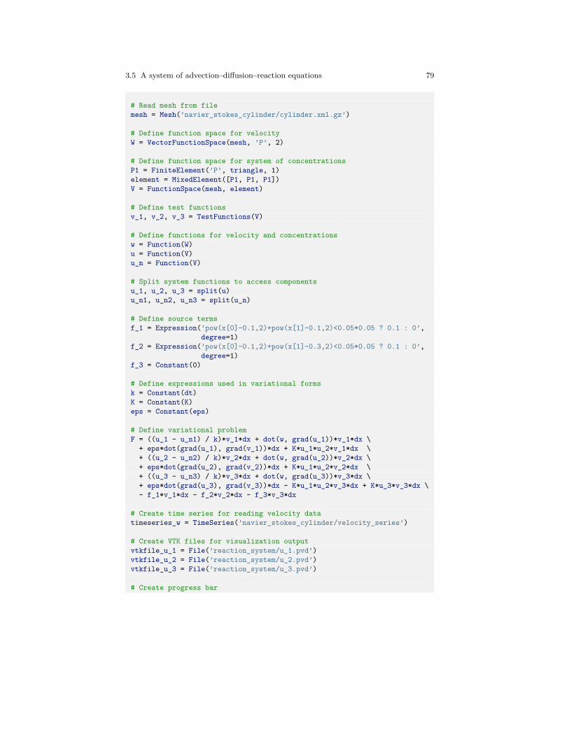
3.5 A system of advection–diffusion–reaction equations 79
# Read mesh from filemesh = Mesh(’navier_stokes_cylinder/cylinder.xml.gz’)
# Define function space for velocityW = VectorFunctionSpace(mesh, ’P’, 2)
# Define function space for system of concentrationsP1 = FiniteElement(’P’, triangle, 1)element = MixedElement([P1, P1, P1])V = FunctionSpace(mesh, element)
# Define test functionsv_1, v_2, v_3 = TestFunctions(V)
# Define functions for velocity and concentrationsw = Function(W)u = Function(V)u_n = Function(V)
# Split system functions to access componentsu_1, u_2, u_3 = split(u)u_n1, u_n2, u_n3 = split(u_n)
# Define source termsf_1 = Expression(’pow(x[0]-0.1,2)+pow(x[1]-0.1,2)<0.05*0.05 ? 0.1 : 0’,
degree=1)f_2 = Expression(’pow(x[0]-0.1,2)+pow(x[1]-0.3,2)<0.05*0.05 ? 0.1 : 0’,
degree=1)f_3 = Constant(0)
# Define expressions used in variational formsk = Constant(dt)K = Constant(K)eps = Constant(eps)
# Define variational problemF = ((u_1 - u_n1) / k)*v_1*dx + dot(w, grad(u_1))*v_1*dx \
+ eps*dot(grad(u_1), grad(v_1))*dx + K*u_1*u_2*v_1*dx \+ ((u_2 - u_n2) / k)*v_2*dx + dot(w, grad(u_2))*v_2*dx \+ eps*dot(grad(u_2), grad(v_2))*dx + K*u_1*u_2*v_2*dx \+ ((u_3 - u_n3) / k)*v_3*dx + dot(w, grad(u_3))*v_3*dx \+ eps*dot(grad(u_3), grad(v_3))*dx - K*u_1*u_2*v_3*dx + K*u_3*v_3*dx \- f_1*v_1*dx - f_2*v_2*dx - f_3*v_3*dx
# Create time series for reading velocity datatimeseries_w = TimeSeries(’navier_stokes_cylinder/velocity_series’)
# Create VTK files for visualization outputvtkfile_u_1 = File(’reaction_system/u_1.pvd’)vtkfile_u_2 = File(’reaction_system/u_2.pvd’)vtkfile_u_3 = File(’reaction_system/u_3.pvd’)
# Create progress bar
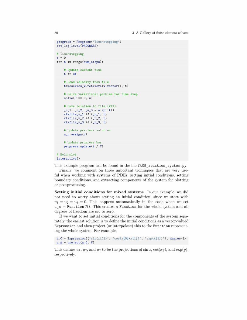
80 3 A Gallery of finite element solvers
progress = Progress(’Time-stepping’)set_log_level(PROGRESS)
# Time-steppingt = 0for n in range(num_steps):
# Update current timet += dt
# Read velocity from filetimeseries_w.retrieve(w.vector(), t)
# Solve variational problem for time stepsolve(F == 0, u)
# Save solution to file (VTK)_u_1, _u_2, _u_3 = u.split()vtkfile_u_1 << (_u_1, t)vtkfile_u_2 << (_u_2, t)vtkfile_u_3 << (_u_3, t)
# Update previous solutionu_n.assign(u)
# Update progress barprogress.update(t / T)
# Hold plotinteractive()
This example program can be found in the file ft09_reaction_system.py.Finally, we comment on three important techniques that are very use-
ful when working with systems of PDEs: setting initial conditions, settingboundary conditions, and extracting components of the system for plottingor postprocessing.
Setting initial conditions for mixed systems. In our example, we didnot need to worry about setting an initial condition, since we start withu1 = u2 = u3 = 0. This happens automatically in the code when we setu_n = Function(V). This creates a Function for the whole system and alldegrees of freedom are set to zero.
If we want to set initial conditions for the components of the system sepa-rately, the easiest solution is to define the initial conditions as a vector-valuedExpression and then project (or interpolate) this to the Function represent-ing the whole system. For example,
u_0 = Expression((’sin(x[0])’, ’cos(x[0]*x[1])’, ’exp(x[1])’), degree=1)u_n = project(u_0, V)
This defines u1, u2, and u2 to be the projections of sinx, cos(xy), and exp(y),respectively.

3.5 A system of advection–diffusion–reaction equations 81
Setting boundary conditions for mixed systems. In our example, wealso did not need to worry about setting boundary conditions since we useda natural Neumann condition. If we want to set Dirichlet conditions for in-dividual components of the system, this can be done as usual by the classDirichletBC, but we must specify for which subsystem we set the bound-ary condition. For example, to specify that u2 should be equal to xy on theboundary defined by boundary, we do
u_D = Expression(’x[0]*x[1]’, degree=1)bc = DirichletBC(V.sub(1), u_D, boundary)
The object bc or a list of such objects containing different boundary condi-tions, can then be passed to the solve function as usual. Note that numberingstarts at 0 in FEniCS so the subspace corresponding to u2 is V.sub(1).
Accessing components of mixed systems. If u is a Function defined ona mixed function space in FEniCS, there are several ways in which u can besplit into components. Above we already saw an example of the first of these:
u_1, u_2, u_3 = split(u)
This extracts the components of u as symbols that can be used in a variationalproblem. The above statement is in fact equivalent to
u_1 = u[0]u_2 = u[1]u_3 = u[2]
Note that u[0] is not really a Function object, but merely a symbolic ex-pression, just like grad(u) in FEniCS is a symbolic expression and not aFunction representing the gradient. This means that u_1, u_2, u_3 can beused in a variational problem, but cannot be used for plotting or postpro-cessing.
To access the components of u for plotting and saving the solution to file,we need to use a different variant of the split function:
u_1_, u_2_, u_3_ = u.split()
This returns three subfunctions as actual objects with access to the commonunderlying data stored in u, which makes plotting and saving to file possible.Alternatively, we can do
u_1_, u_2_, u_3_ = u.split(deepcopy=True)
which will create u_1_, u_2_, and u_3_ as stand-alone Function objects,each holding a copy of the subfunction data extracted from u. This is usefulin many situations but is not necessary for plotting and saving solutions tofile.

Chapter 4Subdomains and boundary conditions
So far, we have only looked briefly at how to specify boundary conditions. In thischapter, we look more closely at how to specify boundary conditions on specificparts (subdomains) of the boundary and how to combine multiple boundary con-ditions. We will also look at how to generate meshes with subdomains and howto define coefficients with different values in different subdomains.
4.1 Combining Dirichlet and Neumannconditions
Let’s return to the Poisson problem from Chapter 2 and see how to extendthe mathematics and the implementation to handle a Dirichlet condition incombination with a Neumann condition. The domain is still the unit square,but now we set the Dirichlet condition u = uD at the left and right sides,x= 0 and x= 1, while the Neumann condition
−∂u∂n
= g
is applied to the remaining sides y = 0 and y = 1.
4.1.1 PDE problem
Let ΓD and ΓN denote the parts of the boundary ∂Ω where the Dirichletand Neumann conditions apply, respectively. The complete boundary-valueproblem can be written as
c© 2017, Hans Petter Langtangen, Anders Logg.Released under CC Attribution 4.0 license
84 4 Subdomains and boundary conditions
−∇2u= f in Ω, (4.1)u= uD on ΓD , (4.2)
−∂u∂n
= g on ΓN . (4.3)
Again, we choose u= 1+x2 +2y2 as the exact solution and adjust f , g, anduD accordingly:
f(x,y) =−6,
g(x,y) =
0, y = 0,−4, y = 1,
uD(x,y) = 1 +x2 + 2y2 .
For ease of programming, we define g as a function over the whole domainΩ such that g takes on the correct values at y = 0 and y = 1. One possibleextension is
g(x,y) =−4y .
4.1.2 Variational formulation
The first task is to derive the variational formulation. This time we cannotomit the boundary term arising from the integration by parts, because v isonly zero on ΓD . We have
−∫Ω
(∇2u)vdx=∫Ω∇u ·∇vdx−
∫∂Ω
∂u
∂nvds,
and since v = 0 on ΓD ,
−∫∂Ω
∂u
∂nvds=−
∫ΓN
∂u
∂nvds=
∫ΓN
gvds,
by applying the boundary condition on ΓN . The resulting weak form reads∫Ω∇u ·∇vdx=
∫Ωfvdx−
∫ΓN
gvds. (4.4)
Expressing this equation in the standard notation a(u,v) = L(v) is straight-forward with

4.1 Combining Dirichlet and Neumann conditions 85
a(u,v) =∫Ω∇u ·∇vdx, (4.5)
L(v) =∫Ωfvdx−
∫ΓN
gvds. (4.6)
4.1.3 FEniCS implementation
How does the Neumann condition impact the implementation? Let us revisitour previous implementation ft01_poisson.py from Section 2.2 and examinewhich changes we need to make to incorporate the Neumann condition. Itturns out that only two changes are necessary:
• The function boundary defining the Dirichlet boundary must be modified.• The new boundary term must be added to the expression for L.
The first adjustment can be coded as
tol = 1E-14
def boundary_D(x, on_boundary):if on_boundary:
if near(x[0], 0, tol) or near(x[0], 1, tol):return True
else:return False
else:return False
A more compact implementation reads
def boundary_D(x, on_boundary):return on_boundary and (near(x[0], 0, tol) or near(x[0], 1, tol))
The second adjustment of our program concerns the definition of L, whichneeds to include the Neumann condition:
g = Expression(’-4*x[1]’, degree=1)L = f*v*dx - g*v*ds
The ds variable implies a boundary integral, while dx implies an integral overthe domain Ω. No other modifications are necessary.
Note that the integration *ds is carried out over the entire boundary,including the Dirichlet boundary. However, since the test function v vanisheson the Dirichlet boundary (as a result specifying a DirichletBC), the integralwill only include the contribution from the Neumann boundary.

86 4 Subdomains and boundary conditions
4.2 Setting multiple Dirichlet conditions
In the previous section, we used a single function uD(x,y) for setting Dirichletconditions on two parts of the boundary. Often it is more practical to usemultiple functions, one for each subdomain of the boundary. Let us return tothe case from Section 4.1 and redefine the problem in terms of two Dirichletconditions:
−∇2u= f in Ω,
u= uL on ΓL
D ,
u= uR on ΓR
D ,
−∂u∂n
= g on ΓN .
Here, Γ L
D is the left boundary x = 0, while ΓR
D is the right boundary x = 1.We note that uL(x,y) = 1 + 2y2, uR(x,y) = 2 + 2y2, and g(x,y) = 4y.
For the boundary condition on Γ L
D , we define the usual triple of an expres-sion for the boundary value, a function defining the location of the boundary,and a DirichletBC object:
u_L = Expression(’1 + 2*x[1]*x[1]’, degree=2)
def boundary_L(x, on_boundary):tol = 1E-14return on_boundary and near(x[0], 0, tol)
bc_L = DirichletBC(V, u_L, boundary_L)
For the boundary condition on ΓR
D , we write a similar code snippet:
u_R = Expression(’2 + 2*x[1]*x[1]’, degree=2)
def boundary_R(x, on_boundary):tol = 1E-14return on_boundary and near(x[0], 1, tol)
bc_R = DirichletBC(V, u_R, boundary_R)
We collect the two boundary conditions in a list which we can pass to thesolve function to compute the solution:
bcs = [bc_L, bc_R]...solve(a == L, u, bcs)
Note that for boundary values that do not depend on x or y, we mightreplace the Expression objects by Constant objects.

4.3 Defining subdomains for different materials 87
4.3 Defining subdomains for different materials
Solving PDEs in domains made up of different materials is a frequently en-countered task. In FEniCS, these kinds of problems are handled by definingsubdomains inside the domain. A simple example with two materials (subdo-mains) in 2D will demonstrate the idea. We consider the following variable-coefficient extension of the Poisson equation from Chapter 2:
−∇· [κ(x,y)∇u(x,y)] = f(x,y), (4.7)
in some domain Ω. Physically, this problem may be viewed as a model ofheat conduction, with variable heat conductivity κ(x,y)≥ κ > 0.
For illustration purposes, we consider the domain Ω = [0,1]× [0,1] anddivide it into two equal subdomains, as depicted in Figure 4.1:
Ω0 = [0,1]× [0,1/2], Ω1 = [0,1]× (1/2,1] .
We define κ(x,y) = κ0 in Ω0 and κ(x,y) = κ1 in Ω1, where κ0,κ1 > 0 aregiven constants.
Fig. 4.1 Two subdomains with different material parameters.
The variational formulation may be easily expressed in FEniCS as follows:
a = kappa*dot(grad(u), grad(v))*dxL = f*v*dx
In the remainder of this section, we will discuss different strategies for definingthe coefficient kappa as an Expression that takes on different values in thetwo subdomains.
88 4 Subdomains and boundary conditions
4.3.1 Using expressions to define subdomains
The simplest way to implement a variable coefficient κ= κ(x,y) is to define anExpression which depends on the coordinates x and y. We have previouslyused the Expression class to define expressions based on simple formulas.Aternatively, an Expression can be defined as a Python class which allows formore complex logic. The following code snippet illustrates this construction:
class K(Expression):def set_k_values(self, k_0, k_1):
self.k_0, self.k_1 = k_0, k_1
def eval(self, value, x):"Set value[0] to value at point x"tol = 1E-14if x[1] <= 0.5 + tol:
value[0] = self.k_0else:
value[0] = self.k_1
# Initialize kappakappa = K(degree=0)kappa.set_k_values(1, 0.01)
The eval method gives great flexibility in defining functions, but a downsideis that FEniCS will call eval in Python for each node x, which is a slowprocess.
An alternative method is to use a C++ string expression as we have seenbefore, which is much more efficient in FEniCS. This can be done using aninline if test:
tol = 1E-14k_0 = 1.0k_1 = 0.01kappa = Expression(’x[1] <= 0.5 + tol ? k_0 : k_1’, degree=0,
tol=tol, k_0=k_0, k_1=k_1)
This method of defining variable coefficients works if the subdomains aresimple shapes that can be expressed in terms of geometric inequalities. How-ever, for more complex subdomains, we will need to use a more general tech-nique, as we will see next.
4.3.2 Using mesh functions to define subdomains
We now address how to specify the subdomains Ω0 and Ω1 using a more gen-eral technique. This technique involves the use of two classes that are essentialin FEniCS when working with subdomains: SubDomain and MeshFunction.Consider the following definition of the boundary x= 0:

4.3 Defining subdomains for different materials 89
def boundary(x, on_boundary):tol = 1E-14return on_boundary and near(x[0], 0, tol)
This boundary definition is actually a shortcut to the more general FEniCSconcept SubDomain. A SubDomain is a class which defines a region in space(a subdomain) in terms of a member function inside which returns True forpoints that belong to the subdomain and False for points that don’t belongto the subdomain. Here is how to specify the boundary x= 0 as a SubDomain:
class Boundary(SubDomain):def inside(self, x, on_boundary):
tol = 1E-14return on_boundary and near(x[0], 0, tol)
boundary = Boundary()bc = DirichletBC(V, Constant(0), boundary)
We notice that the inside function of the class Boundary is (almost) iden-tical to the previous boundary definition in terms of the boundary function.Technically, our class Boundary is a subclass of the FEniCS class SubDomain.
We will use two SubDomain subclasses to define the two subdomains Ω0and Ω1:
tol = 1E-14
class Omega_0(SubDomain):def inside(self, x, on_boundary):
return x[1] <= 0.5 + tol
class Omega_1(SubDomain):def inside(self, x, on_boundary):
return x[1] >= 0.5 - tol
Notice the use of <= and >= in both tests. FEniCS will call the insidefunction for each vertex in a cell to determine whether or not the cell belongsto a particular subdomain. For this reason, it is important that the testholds for all vertices in cells aligned with the boundary. In addition, we use atolerance to make sure that vertices on the internal boundary at y = 0.5 willbelong to both subdomains. This is a little counter-intuitive, but is necessaryto make the cells both above and below the internal boundary belong toeither Ω0 or Ω1.
To define the variable coefficient κ, we will use a powerful tool in FEn-iCS called a MeshFunction. A MeshFunction is a discrete function that canbe evaluated at a set of so-called mesh entities. A mesh entity in FEn-iCS is either a vertex, an edge, a face, or a cell (triangle or tetrahedron).A MeshFunction over cells is suitable to represent subdomains (materials),while a MeshFunction over facets (edges or faces) is used to represent piecesof external or internal boundaries. A MeshFunction over cells can also be usedto represent boundary markers for mesh refinement. A FEniCS MeshFunction

90 4 Subdomains and boundary conditions
is parameterized both over its data type (like integers or booleans) and itsdimension (0 = vertex, 1 = edge etc.). Special subclasses VertexFunction,EdgeFunction etc. are provided for easy definition of a MeshFunction of aparticular dimension.
Since we need to define subdomains of Ω in the present example, we makeuse of a CellFunction. The constructor is given two arguments: (1) the typeof value: ’int’ for integers, ’size_t’ for non-negative (unsigned) integers,’double’ for real numbers, and ’bool’ for logical values; (2) a Mesh ob-ject. Alternatively, the constructor can take just a filename and initialize theCellFunction from data in a file.
We first create a CellFunction with non-negative integer values (’size_t’):
materials = CellFunction(’size_t’, mesh)
Next, we use the two subdomains to mark the cells belonging to eachsubdomain:
subdomain_0 = Omega_0()subdomain_1 = Omega_1()subdomain_0.mark(materials, 0)subdomain_1.mark(materials, 1)
This will set the values of the mesh function materials to 0 on each cellbelonging to Ω0 and 1 on all cells belonging to Ω1. Alternatively, we can usethe following equivalent code to mark the cells:
materials.set_all(0)subdomain_1.mark(materials, 1)
To examine the values of the mesh function and see that we have indeeddefined our subdomains correctly, we can simply plot the mesh function:
plot(materials, interactive=True)
We may also wish to store the values of the mesh function for later use:
File(’materials.xml.gz’) << materials
which can later be read back from file as follows:
File(’materials.xml.gz’) >> materials
Now, to use the values of the mesh function materials to define thevariable coefficient κ, we create a FEniCS Expression:
class K(Expression):def __init__(self, materials, k_0, k_1, **kwargs):
self.materials = materialsself.k_0 = k_0self.k_1 = k_1
def eval_cell(self, values, x, cell):if self.materials[cell.index] == 0:
4.3 Defining subdomains for different materials 91
values[0] = self.k_0else:
values[0] = self.k_1
kappa = K(materials, k_0, k_1, degree=0)
This is similar to the Expression subclass we defined above, but we makeuse of the member function eval_cell in place of the regular eval function.This version of the evaluation function has an additional cell argumentwhich we can use to check on which cell we are currently evaluating thefunction. We also defined the special function __init__ (the constructor) sothat we can pass all data to the Expression when it is created.
Since we make use of geometric tests to define the two SubDomains for Ω0and Ω1, the MeshFunction method may seem like an unnecessary compli-cation of the simple method using an Expression with an if-test. However,in general the definition of subdomains may be available as a MeshFunction(from a data file), perhaps generated as part of the mesh generation process,and not as a simple geometric test. In such cases the method demonstratedhere is the recommended way to work with subdomains.
4.3.3 Using C++ code snippets to define subdomains
The SubDomain and Expression Python classes are very convenient, buttheir use leads to function calls from C++ to Python for each node in themesh. Since this involves a significant cost, we need to make use of C++ codeif performance is an issue.
Instead of writing the SubDomain subclass in Python, we may instead usethe CompiledSubDomain tool in FEniCS to specify the subdomain in C++code and thereby speed up our code. Consider the definition of the classesOmega_0 and Omega_1 above in Python. The key strings that define thesesubdomains can be expressed in C++ syntax and given as arguments toCompiledSubDomain as follows:
tol = 1E-14subdomain_0 = CompiledSubDomain(’x[1] <= 0.5 + tol’, tol=tol)subdomain_1 = CompiledSubDomain(’x[1] >= 0.5 - tol’, tol=tol)
As seen, parameters can be specified using keyword arguments. The resultingobjects, subdomain_0 and subdomain_1, can be used as ordinary SubDomainobjects.
Compiled subdomain strings can be applied for specifying boundaries aswell:
boundary_R = CompiledSubDomain(’on_boundary && near(x[0], 1, tol)’,tol=1E-14)
92 4 Subdomains and boundary conditions
It is also possible to feed the C++ string (without parameters) directlyas the third argument to DirichletBC without explicitly constructing aCompiledSubDomain object:
bc1 = DirichletBC(V, value, ’on_boundary && near(x[0], 1, tol)’)
Python Expression classes may also be redefined using C++ for more ef-ficient code. Consider again the definition of the class K above for the variablecoefficient κ = κ(x). This may be redefined using a C++ code snippet andthe keyword cppcode to the regular FEniCS Expression class:
cppcode = """class K : public Expressionpublic:
void eval(Array<double>& values,const Array<double>& x,const ufc::cell& cell) const
if ((*materials)[cell.index] == 0)
values[0] = k_0;else
values[0] = k_1;
std::shared_ptr<MeshFunction<std::size_t>> materials;double k_0;double k_1;
;"""
kappa = Expression(cppcode=cppcode, degree=0)kappa.materials = materialskappa.k_0 = k_0kappa.k_1 = k_1
4.4 Setting multiple Dirichlet, Neumann, andRobin conditions
Consider again the variable-coefficient Poisson problem from Section 4.3. Wewill now discuss how to implement general combinations of boundary condi-tions of Dirichlet, Neumann, and Robin type for this model problem.
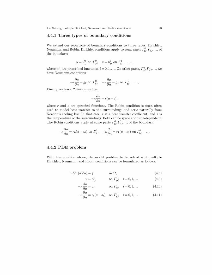
4.4 Setting multiple Dirichlet, Neumann, and Robin conditions 93
4.4.1 Three types of boundary conditions
We extend our repertoire of boundary conditions to three types: Dirichlet,Neumann, and Robin. Dirichlet conditions apply to some parts Γ 0
D ,Γ1D , . . ., of
the boundary:
u= u0D on Γ 0
D , u= u1D on Γ 1
D , . . . ,
where uiD are prescribed functions, i= 0,1, . . .. On other parts, Γ 0N ,Γ
1N , . . ., we
have Neumann conditions:
−κ∂u∂n
= g0 on Γ 0N , −κ
∂u
∂n= g1 on Γ 1
N , . . . ,
Finally, we have Robin conditions:
−κ∂u∂n
= r(u−s),
where r and s are specified functions. The Robin condition is most oftenused to model heat transfer to the surroundings and arise naturally fromNewton’s cooling law. In that case, r is a heat transfer coefficient, and s isthe temperature of the surroundings. Both can be space and time-dependent.The Robin conditions apply at some parts Γ 0
R ,Γ1R , . . ., of the boundary:
−κ∂u∂n
= r0(u−s0) on Γ 0R , −κ
∂u
∂n= r1(u−s1) on Γ 1
R , . . .
4.4.2 PDE problem
With the notation above, the model problem to be solved with multipleDirichlet, Neumann, and Robin conditions can be formulated as follows:
−∇· (κ∇u) = f in Ω, (4.8)u= uiD on Γ iD , i= 0,1, . . . (4.9)
−κ∂u∂n
= gi on Γ iN , i= 0,1, . . . (4.10)
−κ∂u∂n
= ri(u−si) on Γ iR , i= 0,1, . . . (4.11)

94 4 Subdomains and boundary conditions
4.4.3 Variational formulation
As usual, we multiply by a test function v and integrate by parts:
−∫Ω∇· (κ∇u)vdx=
∫Ωκ∇u ·∇vdx−
∫∂Ω
κ∂u
∂nvds.
On the Dirichlet part of the boundary (Γ iD), the boundary integral vanishessince v = 0. On the remaining part of the boundary, we split the boundaryintegral into contributions from the Neumann parts (Γ iN) and Robin parts(Γ iR). Inserting the boundary conditions, we obtain
−∫∂Ω
κ∂u
∂nvds=−
∑i
∫Γ i
N
κ∂u
∂nds−
∑i
∫Γ i
R
κ∂u
∂nds
=∑i
∫Γ i
N
gids+∑i
∫Γ i
R
ri(u−si)ds.
We thus obtain the following variational problem:
F =∫Ωκ∇u ·∇vdx+
∑i
∫Γ i
N
givds+∑i
∫Γ i
R
ri(u−si)vds−∫Ωfvdx= 0 .
(4.12)We have been used to writing this variational formulation in the standard
notation a(u,v) = L(v), which requires that we identify all integral depend-ing on the trial function u, and collect these in a(u,v), while the remainingintegrals go into L(v). The integrals from the Robin condition must for thisreason be split into two parts:∫
Γ iR
ri(u−si)vds=∫Γ i
R
riuvds−∫Γ i
R
risivds.
We then have
a(u,v) =∫Ωκ∇u ·∇vdx+
∑i
∫Γ i
R
riuvds, (4.13)
L(v) =∫Ωfvdx−
∑i
∫Γ i
N
givds+∑i
∫Γ i
R
risivds. (4.14)
Alternatively, we may keep the formulation (4.12) and either solve the varia-tional problem as a nonlinear problem (F == 0) in FEniCS or use the FEniCSfunctions lhs and rhs to extract the bilinear and linear parts of F:
a = lhs(F)

4.4 Setting multiple Dirichlet, Neumann, and Robin conditions 95
L = rhs(F)
Note that if we choose to solve this linear problem as a nonlinear problem,the Newton iteration will converge in a single iteration.
4.4.4 FEniCS implementation
Let us examine how to extend our Poisson solver to handle general combina-tions of Dirichlet, Neumann, and Robin boundary conditions. Compared toour previous code, we must consider the following extensions:
• Defining markers for the different parts of the boundary.• Splitting the boundary integral into parts using the markers.
A general approach to the first task is to mark each of the desired boundaryparts with markers 0, 1, 2, and so forth. Here we aim at the four sides of theunit square, marked with 0 (x= 0), 1 (x= 1), 2 (y = 0), and 3 (y = 1). Themarkers will be defined using a MeshFunction, but contrary to Section 4.3,this is not a function over cells, but a function over the facets of the mesh.We use a FacetFunction for this purpose:
boundary_markers = FacetFunction(’size_t’, mesh)
As in Section 4.3 we use a subclass of SubDomain to identify the variousparts of the mesh function. Problems with domains of more complicatedgeometries may set the mesh function for marking boundaries as part of themesh generation. In our case, the boundary x= 0 can be marked as follows:
class BoundaryX0(SubDomain):tol = 1E-14def inside(self, x, on_boundary):
return on_boundary and near(x[0], 0, tol)
bx0 = BoundaryX0()bx0.mark(boundary_markers, 0)
Similarly, we create the classes BoundaryX1 (x= 1), BoundaryY0 (y= 0), andBoundaryY1 (y = 1) boundary, and mark these as subdomains 1, 2, and 3,respectively.
For generality of the implementation, we let the user specify what kindof boundary condition that applies to each of the four boundaries. We setup a Python dictionary for this purpose, with the key as subdomain numberand the value as a dictionary specifying the kind of condition as key and afunction as its value. For example,
boundary_conditions = 0: ’Dirichlet’: u_D,1: ’Robin’: (r, s),2: ’Neumann’: g,3: ’Neumann’, 0
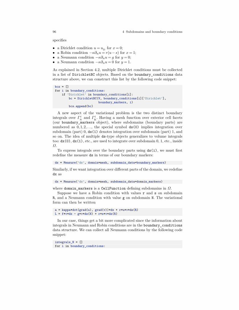
96 4 Subdomains and boundary conditions
specifies
• a Dirichlet condition u= uD for x= 0;• a Robin condition −κ∂nu= r(u−s) for x= 1;• a Neumann condition −κ∂nu= g for y = 0;• a Neumann condition −κ∂nu= 0 for y = 1.
As explained in Section 4.2, multiple Dirichlet conditions must be collectedin a list of DirichletBC objects. Based on the boundary_conditions datastructure above, we can construct this list by the following code snippet:
bcs = []for i in boundary_conditions:
if ’Dirichlet’ in boundary_conditions[i]:bc = DirichletBC(V, boundary_conditions[i][’Dirichlet’],
boundary_markers, i)bcs.append(bc)
A new aspect of the variational problem is the two distinct boundaryintegrals over Γ iN and Γ iR . Having a mesh function over exterior cell facets(our boundary_markers object), where subdomains (boundary parts) arenumbered as 0,1,2, . . ., the special symbol ds(0) implies integration oversubdomain (part) 0, ds(1) denotes integration over subdomain (part) 1, andso on. The idea of multiple ds-type objects generalizes to volume integralstoo: dx(0), dx(1), etc., are used to integrate over subdomain 0, 1, etc., insideΩ.
To express integrals over the boundary parts using ds(i), we must firstredefine the measure ds in terms of our boundary markers:
ds = Measure(’ds’, domain=mesh, subdomain_data=boundary_markers)
Similarly, if we want integration over different parts of the domain, we redefinedx as
dx = Measure(’dx’, domain=mesh, subdomain_data=domain_markers)
where domain_markers is a CellFunction defining subdomains in Ω.Suppose we have a Robin condition with values r and s on subdomain
R, and a Neumann condition with value g on subdomain N. The variationalform can then be written
a = kappa*dot(grad(u), grad(v))*dx + r*u*v*ds(R)L = f*v*dx - g*v*ds(N) + r*s*v*ds(R)
In our case, things get a bit more complicated since the information aboutintegrals in Neumann and Robin conditions are in the boundary_conditionsdata structure. We can collect all Neumann conditions by the following codesnippet:
integrals_N = []for i in boundary_conditions:
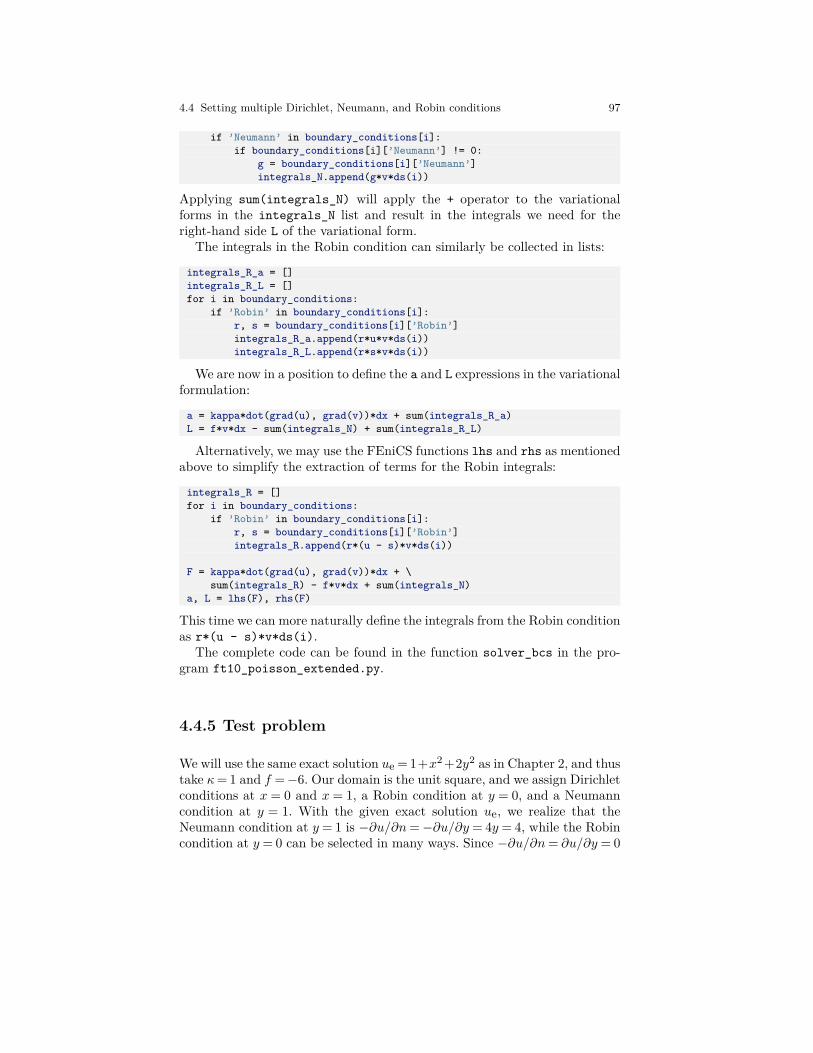
4.4 Setting multiple Dirichlet, Neumann, and Robin conditions 97
if ’Neumann’ in boundary_conditions[i]:if boundary_conditions[i][’Neumann’] != 0:
g = boundary_conditions[i][’Neumann’]integrals_N.append(g*v*ds(i))
Applying sum(integrals_N) will apply the + operator to the variationalforms in the integrals_N list and result in the integrals we need for theright-hand side L of the variational form.
The integrals in the Robin condition can similarly be collected in lists:
integrals_R_a = []integrals_R_L = []for i in boundary_conditions:
if ’Robin’ in boundary_conditions[i]:r, s = boundary_conditions[i][’Robin’]integrals_R_a.append(r*u*v*ds(i))integrals_R_L.append(r*s*v*ds(i))
We are now in a position to define the a and L expressions in the variationalformulation:
a = kappa*dot(grad(u), grad(v))*dx + sum(integrals_R_a)L = f*v*dx - sum(integrals_N) + sum(integrals_R_L)
Alternatively, we may use the FEniCS functions lhs and rhs as mentionedabove to simplify the extraction of terms for the Robin integrals:
integrals_R = []for i in boundary_conditions:
if ’Robin’ in boundary_conditions[i]:r, s = boundary_conditions[i][’Robin’]integrals_R.append(r*(u - s)*v*ds(i))
F = kappa*dot(grad(u), grad(v))*dx + \sum(integrals_R) - f*v*dx + sum(integrals_N)
a, L = lhs(F), rhs(F)
This time we can more naturally define the integrals from the Robin conditionas r*(u - s)*v*ds(i).
The complete code can be found in the function solver_bcs in the pro-gram ft10_poisson_extended.py.
4.4.5 Test problem
We will use the same exact solution ue = 1+x2 +2y2 as in Chapter 2, and thustake κ= 1 and f =−6. Our domain is the unit square, and we assign Dirichletconditions at x = 0 and x = 1, a Robin condition at y = 0, and a Neumanncondition at y = 1. With the given exact solution ue, we realize that theNeumann condition at y = 1 is −∂u/∂n=−∂u/∂y = 4y = 4, while the Robincondition at y = 0 can be selected in many ways. Since −∂u/∂n= ∂u/∂y = 0
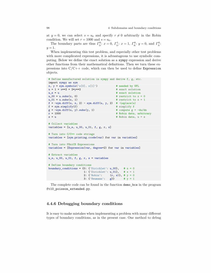
98 4 Subdomains and boundary conditions
at y = 0, we can select s = ue and specify r 6= 0 arbitrarily in the Robincondition. We will set r = 1000 and s= ue.
The boundary parts are thus Γ 0D : x = 0, Γ 1
D : x = 1, Γ 0R : y = 0, and Γ 0
N :y = 1.
When implementing this test problem, and especially other test problemswith more complicated expressions, it is advantageous to use symbolic com-puting. Below we define the exact solution as a sympy expression and deriveother functions from their mathematical definitions. Then we turn these ex-pressions into C/C++ code, which can then be used to define Expressionobjects.
# Define manufactured solution in sympy and derive f, g, etc.import sympy as symx, y = sym.symbols(’x[0], x[1]’) # needed by UFLu = 1 + x**2 + 2*y**2 # exact solutionu_e = u # exact solutionu_00 = u.subs(x, 0) # restrict to x = 0u_01 = u.subs(x, 1) # restrict to x = 1f = -sym.diff(u, x, 2) - sym.diff(u, y, 2) # -Laplace(u)f = sym.simplify(f) # simplify fg = -sym.diff(u, y).subs(y, 1) # compute g = -du/dnr = 1000 # Robin data, arbitrarys = u # Robin data, u = s
# Collect variablesvariables = [u_e, u_00, u_01, f, g, r, s]
# Turn into C/C++ code stringsvariables = [sym.printing.ccode(var) for var in variables]
# Turn into FEniCS Expressionsvariables = [Expression(var, degree=2) for var in variables]
# Extract variablesu_e, u_00, u_01, f, g, r, s = variables
# Define boundary conditionsboundary_conditions = 0: ’Dirichlet’: u_00, # x = 0
1: ’Dirichlet’: u_01, # x = 12: ’Robin’: (r, s), # y = 03: ’Neumann’: g # y = 1
The complete code can be found in the function demo_bcs in the programft10_poisson_extended.py.
4.4.6 Debugging boundary conditions
It is easy to make mistakes when implementing a problem with many differenttypes of boundary conditions, as in the present case. One method to debug
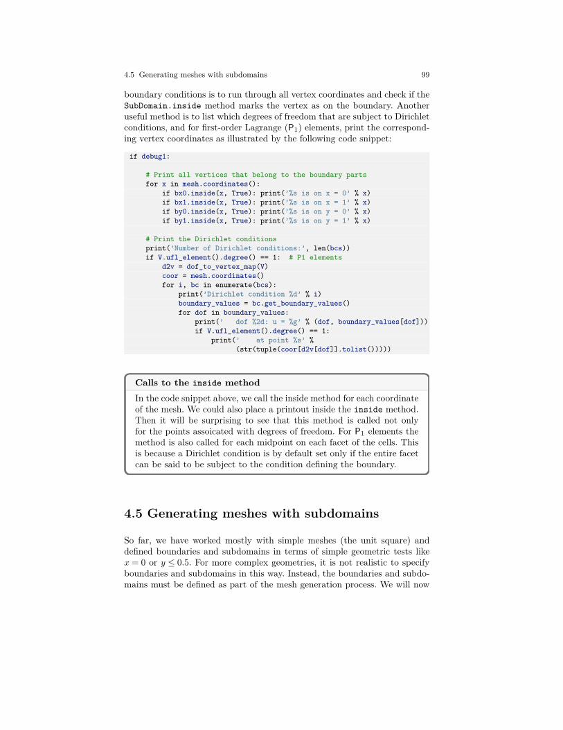
4.5 Generating meshes with subdomains 99
boundary conditions is to run through all vertex coordinates and check if theSubDomain.inside method marks the vertex as on the boundary. Anotheruseful method is to list which degrees of freedom that are subject to Dirichletconditions, and for first-order Lagrange (P1) elements, print the correspond-ing vertex coordinates as illustrated by the following code snippet:
if debug1:
# Print all vertices that belong to the boundary partsfor x in mesh.coordinates():
if bx0.inside(x, True): print(’%s is on x = 0’ % x)if bx1.inside(x, True): print(’%s is on x = 1’ % x)if by0.inside(x, True): print(’%s is on y = 0’ % x)if by1.inside(x, True): print(’%s is on y = 1’ % x)
# Print the Dirichlet conditionsprint(’Number of Dirichlet conditions:’, len(bcs))if V.ufl_element().degree() == 1: # P1 elements
d2v = dof_to_vertex_map(V)coor = mesh.coordinates()for i, bc in enumerate(bcs):
print(’Dirichlet condition %d’ % i)boundary_values = bc.get_boundary_values()for dof in boundary_values:
print(’ dof %2d: u = %g’ % (dof, boundary_values[dof]))if V.ufl_element().degree() == 1:
print(’ at point %s’ %(str(tuple(coor[d2v[dof]].tolist()))))
Calls to the inside methodIn the code snippet above, we call the inside method for each coordinateof the mesh. We could also place a printout inside the inside method.Then it will be surprising to see that this method is called not onlyfor the points assoicated with degrees of freedom. For P1 elements themethod is also called for each midpoint on each facet of the cells. Thisis because a Dirichlet condition is by default set only if the entire facetcan be said to be subject to the condition defining the boundary.
4.5 Generating meshes with subdomains
So far, we have worked mostly with simple meshes (the unit square) anddefined boundaries and subdomains in terms of simple geometric tests likex = 0 or y ≤ 0.5. For more complex geometries, it is not realistic to specifyboundaries and subdomains in this way. Instead, the boundaries and subdo-mains must be defined as part of the mesh generation process. We will now
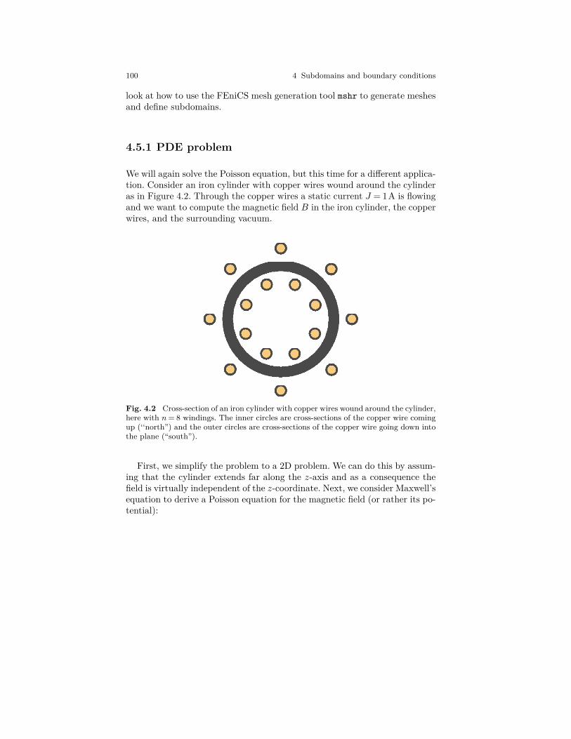
100 4 Subdomains and boundary conditions
look at how to use the FEniCS mesh generation tool mshr to generate meshesand define subdomains.
4.5.1 PDE problem
We will again solve the Poisson equation, but this time for a different applica-tion. Consider an iron cylinder with copper wires wound around the cylinderas in Figure 4.2. Through the copper wires a static current J = 1A is flowingand we want to compute the magnetic field B in the iron cylinder, the copperwires, and the surrounding vacuum.
Fig. 4.2 Cross-section of an iron cylinder with copper wires wound around the cylinder,here with n = 8 windings. The inner circles are cross-sections of the copper wire comingup (‘‘north”) and the outer circles are cross-sections of the copper wire going down intothe plane (“south”).
First, we simplify the problem to a 2D problem. We can do this by assum-ing that the cylinder extends far along the z-axis and as a consequence thefield is virtually independent of the z-coordinate. Next, we consider Maxwell’sequation to derive a Poisson equation for the magnetic field (or rather its po-tential):
4.5 Generating meshes with subdomains 101
∇·D = %, (4.15)∇·B = 0, (4.16)
∇×E =−∂B∂t, (4.17)
∇×H = ∂D
∂t+J. (4.18)
Here, D is the displacement field, B is the magnetic field, E is the electricfield, and H is the magnetizing field. In addition to Maxwell’s equations, wealso need a constitutive relation between B and H,
B = µH, (4.19)
which holds for an isotropic linear magnetic medium. Here, µ is the magneticpermeability of the material. Now, since B is solenoidal (divergence free)according to Maxwell’s equations, we know that B must be the curl of somevector field A. This field is called the magnetic vector potential. Since theproblem is static and thus ∂D/∂t= 0, it follows that
J =∇×H =∇× (µ−1B) =∇× (µ−1∇×A) =−∇· (µ−1∇A). (4.20)
In the last step, we have expanded the second derivatives and used the gaugefreedom of A to simplify the equations to a simple vector-valued Poissonproblem for the magnetic vector potential; if B =∇×A, then B =∇× (A+∇ψ) for any scalar field ψ (the gauge function). For the current problem, wethus need to solve the following 2D Poisson problem for the z-component Azof the magnetic vector potential:
−∇· (µ−1∇Az) = Jz in R2, (4.21)lim
|(x,y)|→∞Az = 0. (4.22)
Since we cannot solve this problem on an infinite domain, we will truncatethe domain using a large disk and set Az = 0 on the boundary. The currentJz is set to +1A in the interior set of circles (copper wire cross-sections) andto −1A in the exterior set of circles in Figure 4.2.
Once the magnetic vector potential has been computed, we can computethe magnetic field B =B(x,y) by
B(x,y) =(∂Az∂y
,−∂Az∂x
). (4.23)

102 4 Subdomains and boundary conditions
4.5.2 Variational formulation
The variational problem is derived as before by multiplying the PDE with atest function v and integrating by parts. Since the boundary integral vanishesdue to the Dirichlet condition, we obtain∫
Ωµ−1∇Az ·∇vdx=
∫ΩJzvdx, (4.24)
or, in other words, a(Az,v) = L(v) with
a(Az,v) =∫Ωµ−1∇Az ·∇vdx, (4.25)
L(v) =∫ΩJzvdx. (4.26)
4.5.3 FEniCS implementation
The first step is to generate a mesh for the geometry described in Figure 4.2.We let a and b be the inner and outer radii of the iron cylinder and let c1and c2 be the radii of the two concentric distributions of copper wire cross-sections. Furthermore, we let r be the radius of a copper wire, R be theradius of our domain, and n be the number of windings (giving a total of2n copper-wire cross-sections). This geometry can be described easily usingmshr and a little bit of Python programming:
# Define geometry for backgrounddomain = Circle(Point(0, 0), R)
# Define geometry for iron cylindercylinder = Circle(Point(0, 0), b) - Circle(Point(0, 0), a)
# Define geometry for wires (N = North (up), S = South (down))angles_N = [i*2*pi/n for i in range(n)]angles_S = [(i + 0.5)*2*pi/n for i in range(n)]wires_N = [Circle(Point(c_1*cos(v), c_1*sin(v)), r) for v in angles_N]wires_S = [Circle(Point(c_2*cos(v), c_2*sin(v)), r) for v in angles_S]
The mesh that we generate will be a mesh of the entire disk with radiusR but we need the mesh generation to respect the internal boundaries de-fined by the iron cylinder and the copper wires. We also want mshr to labelthe subdomains so that we can easily specify material parameters (µ) andcurrents. To do this, we use the mshr function set_subdomain as follows:
# Set subdomain for iron cylinderdomain.set_subdomain(1, cylinder)

4.5 Generating meshes with subdomains 103
# Set subdomains for wiresfor (i, wire) in enumerate(wires_N):
domain.set_subdomain(2 + i, wire)for (i, wire) in enumerate(wires_S):
domain.set_subdomain(2 + n + i, wire)
Once the subdomains have been created, we can generate the mesh:
mesh = generate_mesh(domain, 32)
A detail of the mesh is shown in Figure 4.3.
Fig. 4.3 Plot of (part of) the mesh generated for the magnetostatics test problem. Thesubdomains for the iron cylinder and copper wires are clearly visible.
The mesh generated with mshr will contain information about the sub-domains we have defined. To use this information in the definition of ourvariational problem and subdomain-dependent parameters, we will need tocreate a MeshFunction that marks the subdomains. This can be easily createdby a call to the member function mesh.domains, which holds the subdomaindata generated by mshr:
markers = MeshFunction(’size_t’, mesh, 2, mesh.domains())
This line creates a MeshFunction with unsigned integer values (the subdo-main numbers) with dimension 2, which is the cell dimension for this 2Dproblem.
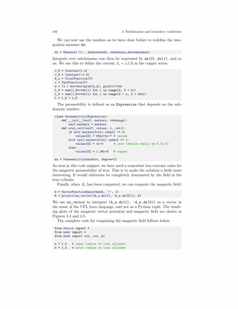
104 4 Subdomains and boundary conditions
We can now use the markers as we have done before to redefine the inte-gration measure dx:
dx = Measure(’dx’, domain=mesh, subdomain_data=markers)
Integrals over subdomains can then be expressed by dx(0), dx(1), and soon. We use this to define the current Jz =±1A in the copper wires:
J_N = Constant(1.0)J_S = Constant(-1.0)A_z = TrialFunction(V)v = TestFunction(V)a = (1 / mu)*dot(grad(A_z), grad(v))*dxL_N = sum(J_N*v*dx(i) for i in range(2, 2 + n))L_S = sum(J_S*v*dx(i) for i in range(2 + n, 2 + 2*n))L = L_N + L_S
The permeability is defined as an Expression that depends on the sub-domain number:
class Permeability(Expression):def __init__(self, markers, **kwargs):
self.markers = markersdef eval_cell(self, values, x, cell):
if self.markers[cell.index] == 0:values[0] = 4*pi*1e-7 # vacuum
elif self.markers[cell.index] == 1:values[0] = 1e-5 # iron (should really be 6.3e-3)
else:values[0] = 1.26e-6 # copper
mu = Permeability(markers, degree=1)
As seen in this code snippet, we have used a somewhat less extreme value forthe magnetic permeability of iron. This is to make the solution a little moreinteresting. It would otherwise be completely dominated by the field in theiron cylinder.
Finally, when Az has been computed, we can compute the magnetic field:
W = VectorFunctionSpace(mesh, ’P’, 1)B = project(as_vector((A_z.dx(1), -A_z.dx(0))), W)
We use as_vector to interpret (A_z.dx(1), -A_z.dx(0)) as a vector inthe sense of the UFL form language, and not as a Python tuple. The result-ing plots of the magnetic vector potential and magnetic field are shown inFigures 4.4 and 4.5.
The complete code for computing the magnetic field follows below.
from fenics import *from mshr import *from math import sin, cos, pi
a = 1.0 # inner radius of iron cylinderb = 1.2 # outer radius of iron cylinder
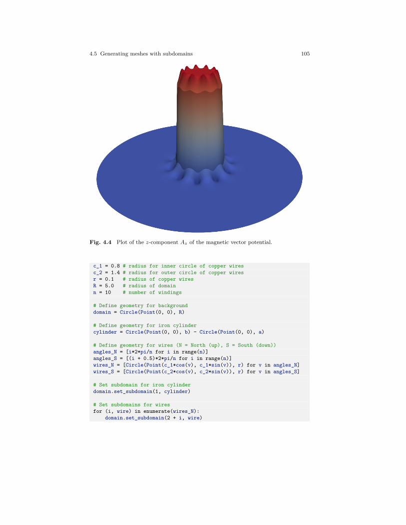
4.5 Generating meshes with subdomains 105
Fig. 4.4 Plot of the z-component Az of the magnetic vector potential.
c_1 = 0.8 # radius for inner circle of copper wiresc_2 = 1.4 # radius for outer circle of copper wiresr = 0.1 # radius of copper wiresR = 5.0 # radius of domainn = 10 # number of windings
# Define geometry for backgrounddomain = Circle(Point(0, 0), R)
# Define geometry for iron cylindercylinder = Circle(Point(0, 0), b) - Circle(Point(0, 0), a)
# Define geometry for wires (N = North (up), S = South (down))angles_N = [i*2*pi/n for i in range(n)]angles_S = [(i + 0.5)*2*pi/n for i in range(n)]wires_N = [Circle(Point(c_1*cos(v), c_1*sin(v)), r) for v in angles_N]wires_S = [Circle(Point(c_2*cos(v), c_2*sin(v)), r) for v in angles_S]
# Set subdomain for iron cylinderdomain.set_subdomain(1, cylinder)
# Set subdomains for wiresfor (i, wire) in enumerate(wires_N):
domain.set_subdomain(2 + i, wire)
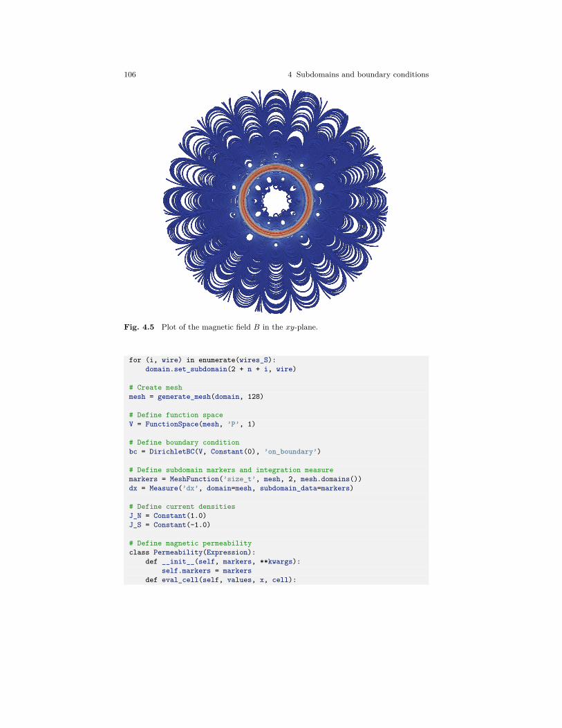
106 4 Subdomains and boundary conditions
Fig. 4.5 Plot of the magnetic field B in the xy-plane.
for (i, wire) in enumerate(wires_S):domain.set_subdomain(2 + n + i, wire)
# Create meshmesh = generate_mesh(domain, 128)
# Define function spaceV = FunctionSpace(mesh, ’P’, 1)
# Define boundary conditionbc = DirichletBC(V, Constant(0), ’on_boundary’)
# Define subdomain markers and integration measuremarkers = MeshFunction(’size_t’, mesh, 2, mesh.domains())dx = Measure(’dx’, domain=mesh, subdomain_data=markers)
# Define current densitiesJ_N = Constant(1.0)J_S = Constant(-1.0)
# Define magnetic permeabilityclass Permeability(Expression):
def __init__(self, markers, **kwargs):self.markers = markers
def eval_cell(self, values, x, cell):
4.5 Generating meshes with subdomains 107
if self.markers[cell.index] == 0:values[0] = 4*pi*1e-7 # vacuum
elif self.markers[cell.index] == 1:values[0] = 1e-5 # iron (should really be 6.3e-3)
else:values[0] = 1.26e-6 # copper
mu = Permeability(markers, degree=1)
# Define variational problemA_z = TrialFunction(V)v = TestFunction(V)a = (1 / mu)*dot(grad(A_z), grad(v))*dxL_N = sum(J_N*v*dx(i) for i in range(2, 2 + n))L_S = sum(J_S*v*dx(i) for i in range(2 + n, 2 + 2*n))L = L_N + L_S
# Solve variational problemA_z = Function(V)solve(a == L, A_z, bc)
# Compute magnetic field (B = curl A)W = VectorFunctionSpace(mesh, ’P’, 1)B = project(as_vector((A_z.dx(1), -A_z.dx(0))), W)
# Plot solutionplot(A_z)plot(B)
# Save solution to filevtkfile_A_z = File(’magnetostatics/potential.pvd’)vtkfile_B = File(’magnetostatics/field.pvd’)vtkfile_A_z << A_zvtkfile_B << B
# Hold plotinteractive()
This example program can be found in the file ft11_magnetostatics.py.

Chapter 5Extensions: Improving the Poissonsolver
The FEniCS programs we have written so far have been designed as flat Pythonscripts. This works well for solving simple demo problems. However, when youbuild a solver for an advanced application, you will quickly find the need for morestructured programming. In particular, you may want to reuse your solver to solvea large number of problems where you vary the boundary conditions, the domain,and coefficients such as material parameters. In this chapter, we will see how towrite general solver functions to improve the usability of FEniCS programs. Wewill also discuss how to utilize iterative solvers with preconditioners for solvinglinear systems, how to compute derived quantities, such as, e.g., the flux on a partof the boundary, and how to compute errors and convergence rates.
5.1 Refactoring the Poisson solver
Most programs discussed in this book are “flat”; that is, they are not orga-nized into logical, reusable units in terms of Python functions. Such flat pro-grams are useful for quickly testing ideas and sketching solution algorithms,but are not well suited for serious problem solving. We shall therefore lookat how to refactor the Poisson solver from Chapter 2. For a start, this meanssplitting the code into functions. But refactoring is not just a reordering ofexisting statements. During refactoring, we also try to make the functionswe create as reusable as possible in other contexts. We will also encapsu-late statements specific to a certain problem into (non-reusable) functions.Being able to distinguish reusable code from specialized code is a key issuewhen refactoring code, and this ability depends on a good mathematical un-derstanding of the problem at hand (what is general, what is special?). Ina flat program, general and specialized code (and mathematics) are oftenmixed together, which tends to give a blurred understanding of the problemat hand.
c© 2017, Hans Petter Langtangen, Anders Logg.Released under CC Attribution 4.0 license

110 5 Extensions: Improving the Poisson solver
5.1.1 A more general solver function
We consider the flat program ft01_poisson.py for solving the Poisson prob-lem developed in Chapter 2. Some of the code in this program is needed tosolve any Poisson problem −∇2u = f on [0,1]× [0,1] with u = uD on theboundary, while other statements arise from our simple test problem. Letus collect the general, reusable code in a function called solver. Our spe-cial test problem will then just be an application of our solver with someadditional statements. We limit the solver function to just compute the nu-merical solution. Plotting and comparing the solution with the exact solutionare considered to be problem-specific activities to be performed elsewhere.
We parameterize solver by f , uD , and the resolution of the mesh. Sinceit is so trivial to use higher-order finite element functions by changing thethird argument to FunctionSpace, we also add the polynomial degree of thefinite element function space as an argument to solver.
from fenics import *import numpy as np
def solver(f, u_D, Nx, Ny, degree=1):"""Solve -Laplace(u) = f on [0,1] x [0,1] with 2*Nx*Ny Lagrangeelements of specified degree and u = u_D (Expresssion) onthe boundary."""
# Create mesh and define function spacemesh = UnitSquareMesh(Nx, Ny)V = FunctionSpace(mesh, ’P’, degree)
# Define boundary conditiondef boundary(x, on_boundary):
return on_boundary
bc = DirichletBC(V, u_D, boundary)
# Define variational problemu = TrialFunction(V)v = TestFunction(V)a = dot(grad(u), grad(v))*dxL = f*v*dx
# Compute solutionu = Function(V)solve(a == L, u, bc)
return u
The remaining tasks of our initial program, such as calling the solverfunction with problem-specific parameters and plotting, can be placed in
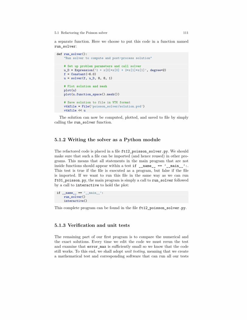
5.1 Refactoring the Poisson solver 111
a separate function. Here we choose to put this code in a function namedrun_solver:
def run_solver():"Run solver to compute and post-process solution"
# Set up problem parameters and call solveru_D = Expression(’1 + x[0]*x[0] + 2*x[1]*x[1]’, degree=2)f = Constant(-6.0)u = solver(f, u_D, 8, 8, 1)
# Plot solution and meshplot(u)plot(u.function_space().mesh())
# Save solution to file in VTK formatvtkfile = File(’poisson_solver/solution.pvd’)vtkfile << u
The solution can now be computed, plotted, and saved to file by simplycalling the run_solver function.
5.1.2 Writing the solver as a Python module
The refactored code is placed in a file ft12_poisson_solver.py. We shouldmake sure that such a file can be imported (and hence reused) in other pro-grams. This means that all statements in the main program that are notinside functions should appear within a test if __name__ == ’__main__’:.This test is true if the file is executed as a program, but false if the fileis imported. If we want to run this file in the same way as we can runft01_poisson.py, the main program is simply a call to run_solver followedby a call to interactive to hold the plot:
if __name__ == ’__main__’:run_solver()interactive()
This complete program can be found in the file ft12_poisson_solver.py.
5.1.3 Verification and unit tests
The remaining part of our first program is to compare the numerical andthe exact solutions. Every time we edit the code we must rerun the testand examine that error_max is sufficiently small so we know that the codestill works. To this end, we shall adopt unit testing, meaning that we createa mathematical test and corresponding software that can run all our tests

112 5 Extensions: Improving the Poisson solver
automatically and check that all tests pass. Python has several tools for unittesting. Two very popular ones are pytest and nose. These are almost identicaland very easy to use. More classical unit testing with test classes is offered bythe built-in module unittest, but here we are going to use pytest (or nose)since that will result in shorter and clearer code.
Mathematically, our unit test is that the finite element solution of ourproblem when f =−6 equals the exact solution u= uD = 1+x2 +2y2 at thevertices of the mesh. We have already created a code that finds the errorat the vertices for our numerical solution. Because of rounding errors, wecannot demand this error to be zero, but we have to use a tolerance, whichdepends on the number of elements and the degrees of the polynomials inthe finite element basis. If we want to test that the solver function worksfor meshes up to 2× (20×20) elements and cubic Lagrange elements, 10−10
is an appropriate tolerance for testing that the maximum error vanishes.To make our test case work together with pytest and nose, we have to
make a couple of small adjustments to our program. The simple rule is thateach test must be placed in a function that
• has a name starting with test_,• has no arguments, and• implements a test expressed as assert success, msg.
Regarding the last point, success is a boolean expression that is False ifthe test fails, and in that case the string msg is written to the screen. Whenthe test fails, assert raises an AssertionError exception in Python, andotherwise runs silently. The msg string is optional, so assert success is theminimal test. In our case, we will write assert error_max < tol, where tolis the tolerance mentioned above.
A proper test function for implementing this unit test in the pytest or nosetesting frameworks has the following form. Note that we perform the test fordifferent mesh resolutions and degrees of finite elements.
def test_solver():"Test solver by reproducing u = 1 + x^2 + 2y^2"
# Set up parameters for testingtol = 1E-10u_D = Expression(’1 + x[0]*x[0] + 2*x[1]*x[1]’, degree=2)f = Constant(-6.0)
# Iterate over mesh sizes and degreesfor Nx, Ny in [(3, 3), (3, 5), (5, 3), (20, 20)]:
for degree in 1, 2, 3:print(’Solving on a 2 x (%d x %d) mesh with P%d elements.’
% (Nx, Ny, degree))
# Compute solutionu = solver(f, u_D, Nx, Ny, degree)
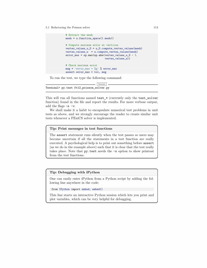
5.1 Refactoring the Poisson solver 113
# Extract the meshmesh = u.function_space().mesh()
# Compute maximum error at verticesvertex_values_u_D = u_D.compute_vertex_values(mesh)vertex_values_u = u.compute_vertex_values(mesh)error_max = np.max(np.abs(vertex_values_u_D - \
vertex_values_u))
# Check maximum errormsg = ’error_max = %g’ % error_maxassert error_max < tol, msg
To run the test, we type the following command:Terminal
Terminal> py.test ft12_poisson_solver.py
This will run all functions named test_* (currently only the test_solverfunction) found in the file and report the results. For more verbose output,add the flags -s -v.
We shall make it a habit to encapsulate numerical test problems in unittests as above, and we strongly encourage the reader to create similar unittests whenever a FEniCS solver is implemented.
Tip: Print messages in test functions
The assert statement runs silently when the test passes so users maybecome uncertain if all the statements in a test function are reallyexecuted. A psychological help is to print out something before assert(as we do in the example above) such that it is clear that the test reallytakes place. Note that py.test needs the -s option to show printoutfrom the test functions.
Tip: Debugging with iPython
One can easily enter iPython from a Python script by adding the fol-lowing line anywhere in the code:
from IPython import embed; embed()
This line starts an interactive Python session which lets you print andplot variables, which can be very helpful for debugging.

114 5 Extensions: Improving the Poisson solver
5.1.4 Parameterizing the number of space dimensions
FEniCS makes it is easy to write a unified simulation code that can op-erate in 1D, 2D, and 3D. As an appetizer, go back to the previous pro-grams ft01_poisson.py or ft12_poisson_solver.py and change the meshconstruction from UnitSquareMesh(8, 8) to UnitCubeMesh(8, 8, 8). Nowthe domain is the unit cube partitioned into 8× 8× 8 boxes, and each boxis divided into six tetrahedron-shaped finite elements for computations. Runthe program and observe that we can solve a 3D problem without any othermodifications! (In 1D, expressions must be modified to not depend on x[1].)The visualization allows you to rotate the cube and observe the functionvalues as colors on the boundary.
If we want to parameterize the creation of unit interval, unit square, or unitcube over dimension, we can do so by encapsulating this part of the code in afunction. Given a list or tuple specifying the division into cells in the spatialcoordinates, the following function returns the mesh for a d-dimensional cube:
def UnitHyperCube(divisions):mesh_classes = [UnitIntervalMesh, UnitSquareMesh, UnitCubeMesh]d = len(divisions)mesh = mesh_classes[d - 1](*divisions)return mesh
The construction mesh_class[d - 1] will pick the right name of the objectused to define the domain and generate the mesh. Moreover, the argument*divisions sends all the components of the list divisions as separate ar-guments to the constructor of the mesh construction class picked out bymesh_class[d - 1]. For example, in a 2D problem where divisions hastwo elements, the statement
mesh = mesh_classes[d - 1](*divisions)
is equivalent to
mesh = UnitSquareMesh(divisions[0], divisions[1])
The solver function from ft12_poisson_solver.py may be modifiedto solve d-dimensional problems by replacing the Nx and Ny parameters bydivisions, and calling the function UnitHyperCube to create the mesh. Notethat UnitHyperCube is a function and not a class, but we have named it usingso-called CamelCase notation to make it look like a class:
mesh = UnitHyperCube(divisions)
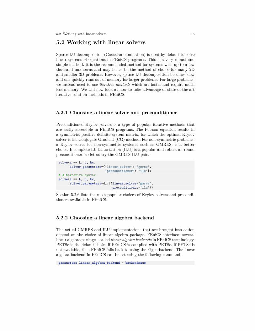
5.2 Working with linear solvers 115
5.2 Working with linear solvers
Sparse LU decomposition (Gaussian elimination) is used by default to solvelinear systems of equations in FEniCS programs. This is a very robust andsimple method. It is the recommended method for systems with up to a fewthousand unknowns and may hence be the method of choice for many 2Dand smaller 3D problems. However, sparse LU decomposition becomes slowand one quickly runs out of memory for larger problems. For large problems,we instead need to use iterative methods which are faster and require muchless memory. We will now look at how to take advantage of state-of-the-artiterative solution methods in FEniCS.
5.2.1 Choosing a linear solver and preconditioner
Preconditioned Krylov solvers is a type of popular iterative methods thatare easily accessible in FEniCS programs. The Poisson equation results ina symmetric, positive definite system matrix, for which the optimal Krylovsolver is the Conjugate Gradient (CG) method. For non-symmetric problems,a Krylov solver for non-symmetric systems, such as GMRES, is a betterchoice. Incomplete LU factorization (ILU) is a popular and robust all-roundpreconditioner, so let us try the GMRES-ILU pair:
solve(a == L, u, bc,solver_parameters=’linear_solver’: ’gmres’,
’preconditioner’: ’ilu’)# Alternative syntaxsolve(a == L, u, bc,
solver_parameters=dict(linear_solver=’gmres’,preconditioner=’ilu’))
Section 5.2.6 lists the most popular choices of Krylov solvers and precondi-tioners available in FEniCS.
5.2.2 Choosing a linear algebra backend
The actual GMRES and ILU implementations that are brought into actiondepend on the choice of linear algebra package. FEniCS interfaces severallinear algebra packages, called linear algebra backends in FEniCS terminology.PETSc is the default choice if FEniCS is compiled with PETSc. If PETSc isnot available, then FEniCS falls back to using the Eigen backend. The linearalgebra backend in FEniCS can be set using the following command:
parameters.linear_algebra_backend = backendname
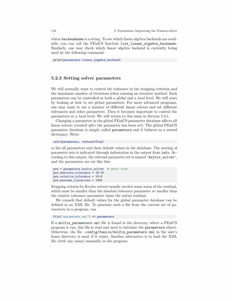
116 5 Extensions: Improving the Poisson solver
where backendname is a string. To see which linear algebra backends are avail-able, you can call the FEniCS function list_linear_algebra_backends.Similarly, one may check which linear algebra backend is currently beingused by the following command:
print(parameters.linear_algebra_backend)
5.2.3 Setting solver parameters
We will normally want to control the tolerance in the stopping criterion andthe maximum number of iterations when running an iterative method. Suchparameters can be controlled at both a global and a local level. We will startby looking at how to set global parameters. For more advanced programs,one may want to use a number of different linear solvers and set differenttolerances and other parameters. Then it becomes important to control theparameters at a local level. We will return to this issue in Section 5.3.1.
Changing a parameter in the global FEniCS parameter database affects alllinear solvers (created after the parameter has been set). The global FEniCSparameter database is simply called parameters and it behaves as a nesteddictionary. Write
info(parameters, verbose=True)
to list all parameters and their default values in the database. The nesting ofparameter sets is indicated through indentation in the output from info. Ac-cording to this output, the relevant parameter set is named ’krylov_solver’,and the parameters are set like this:
prm = parameters.krylov_solver # short formprm.absolute_tolerance = 1E-10prm.relative_tolerance = 1E-6prm.maximum_iterations = 1000
Stopping criteria for Krylov solvers usually involve some norm of the residual,which must be smaller than the absolute tolerance parameter or smaller thanthe relative tolerance parameter times the initial residual.
We remark that default values for the global parameter database can bedefined in an XML file. To generate such a file from the current set of pa-rameters in a program, run
File(’parameters.xml’) << parameters
If a dolfin_parameters.xml file is found in the directory where a FEniCSprogram is run, this file is read and used to initialize the parameters object.Otherwise, the file .config/fenics/dolfin_parameters.xml in the user’shome directory is read, if it exists. Another alternative is to load the XMLfile (with any name) manually in the program:
5.2 Working with linear solvers 117
File(’parameters.xml’) >> parameters
The XML file can also be in gzip’ed form with the extension .xml.gz.
5.2.4 An extended solver function
We may extend the previous solver function from ft12_poisson_solver.pyin Section 5.1.1 such that it also offers the GMRES+ILU preconditionedKrylov solver:
This new solver function, found in the file ft10_poisson_extended.py,replaces the one in ft12_poisson_solver.py. It has all the functionalityof the previous solver function, but can also solve the linear system withiterative methods.
5.2.5 A remark regarding unit tests
Regarding verification of the new solver function in terms of unit tests,it turns out that unit testing for a problem where the approximation errorvanishes gets more complicated when we use iterative methods. The problemis to keep the error due to iterative solution smaller than the tolerance usedin the verification tests. First of all, this means that the tolerances used in theKrylov solvers must be smaller than the tolerance used in the assert test,but this is no guarantee to keep the linear solver error this small. For linearelements and small meshes, a tolerance of 10−11 works well in the case ofKrylov solvers too (using a tolerance 10−12 in those solvers). The interestedreader is referred to the demo_solvers function in ft10_poisson_extended.py for details: this function tests the numerical solution for direct and iterativelinear solvers, for different meshes, and different degrees of the polynomialsin the finite element basis functions.
5.2.6 List of linear solver methods and preconditioners
Which linear solvers and preconditioners that are available in FEniCS de-pends on how FEniCS has been configured and which linear algebra backendis currently active. The following table shows an example of which linearsolvers that can be available through FEniCS when the PETSc backend isactive:

118 5 Extensions: Improving the Poisson solver
Name Method
’bicgstab’ Biconjugate gradient stabilized method’cg’ Conjugate gradient method’gmres’ Generalized minimal residual method’minres’ Minimal residual method’petsc’ PETSc built in LU solver’richardson’ Richardson method’superlu_dist’ Parallel SuperLU’tfqmr’ Transpose-free quasi-minimal residual method’umfpack’ UMFPACK
The set of available preconditioners also depends on configuration and linearalgebra backend. The following table shows an example of which precondi-tioners may be available:
Name Method
’icc’ Incomplete Cholesky factorization’ilu’ Incomplete LU factorization’petsc_amg’ PETSc algebraic multigrid’sor’ Successive over-relaxation
An up-to-date list of the available solvers and preconditioners for your FEn-iCS installation can be produced by
list_linear_solver_methods()list_krylov_solver_preconditioners()
5.3 High-level and low-level solver interfaces
The FEniCS interface allows different ways to access the core functionality,ranging from very high-level to low-level access. So far, we have mostly usedthe high-level call solve(a == L, u, bc) to solve a variational problem a== L with a certain boundary condition bc. However, sometimes you mayneed more fine-grained control of the solution process. In particular, the callto solve will create certain objects that are thrown away after the solutionhas been computed, and it may be practical or efficient to reuse those objects.
5.3.1 Linear variational problem and solver objects
In this section, we will look at an alternative interface to solving linear varia-tional problems in FEniCS, which may be preferable in many situations com-
5.3 High-level and low-level solver interfaces 119
pared to the high-level solve function interface. This interface uses the twoclasses LinearVariationalProblem and LinearVariationalSolver. Usingthis interface, the equivalent of solve(a == L, u, bc) looks as follows:
u = Function(V)problem = LinearVariationalProblem(a, L, u, bc)solver = LinearVariationalSolver(problem)solver.solve()
Many FEniCS objects have an attribute parameters, similar to the globalparameters database, but local to the object. Here, solver.parameters playthat role. Setting the CG method with ILU preconditioning as the solutionmethod and specifying solver-specific parameters can be done like this:
solver.parameters.linear_solver = ’gmres’solver.parameters.preconditioner = ’ilu’prm = solver.parameters.krylov_solver # short formprm.absolute_tolerance = 1E-7prm.relative_tolerance = 1E-4prm.maximum_iterations = 1000
Settings in the global parameters database are propagated to parameter setsin individual objects, with the possibility of being overwritten as above. Notethat global parameter values can only affect local parameter values if setbefore the time of creation of the local object. Thus, changing the value ofthe tolerance in the global parameter database will not affect the parametersfor already created solvers.
5.3.2 Explicit assembly and solve
As we saw already in Section 3.4, linear variational problems can be as-sembled explicitly in FEniCS into matrices and vectors using the assemblefunction. This allows even more fine-grained control of the solution pro-cess compared to using the high-level solve function or using the classesLinearVariationalProblem and LinearVariationalSolver. We will nowlook more closely into how to use the assemble function and how to combinethis with low-level calls for solving the assembled linear systems.
Given a variational problem a(u,v) = L(v), the discrete solution u is com-puted by inserting u=
∑Nj=1Ujφj into a(u,v) and demanding a(u,v) = L(v)
to be fulfilled for N test functions φ1, . . . , φN . This implies
N∑j=1
a(φj , φi)Uj = L(φi), i= 1, . . . ,N,
which is nothing but a linear system,
120 5 Extensions: Improving the Poisson solver
AU = b,
where the entries of A and b are given by
Aij = a(φj , φi),bi = L(φi) .
The examples so far have specified the left- and right-hand sides of thevariational formulation and then asked FEniCS to assemble the linear systemand solve it. An alternative is to explicitly call functions for assembling thecoefficient matrix A and the right-hand side vector b, and then solve thelinear system AU = b for the vector U . Instead of solve(a == L, U, b) wenow write
A = assemble(a)b = assemble(L)bc.apply(A, b)u = Function(V)U = u.vector()solve(A, U, b)
The variables a and L are the same as before; that is, a refers to the bilinearform involving a TrialFunction object u and a TestFunction object v, andL involves the same TestFunction object v. From a and L, the assemblefunction can compute A and b.
Creating the linear system explicitly in a program can have some advan-tages in more advanced problem settings. For example, A may be constantthroughout a time-dependent simulation, so we can avoid recalculating A atevery time level and save a significant amount of simulation time.
The matrix A and vector b are first assembled without incorporating es-sential (Dirichlet) boundary conditions. Thereafter, the call bc.apply(A,b) performs the necessary modifications of the linear system such that u isguaranteed to equal the prescribed boundary values. When we have multipleDirichlet conditions stored in a list bcs, we must apply each condition in bcsto the system:
for bc in bcs:bc.apply(A, b)
# Alternative syntax using list comprehension[bc.apply(A, b) for bc in bcs]
Alternatively, we can use the function assemble_system, which takes theboundary conditions into account when assembling the linear system. Thismethod preserves the symmetry of the linear system for a symmetric bilinearform. Even if the matrix A that comes out of the call to assemble is sym-metric (for a symmetric bilinear form a), the call to bc.apply will break thesymmetry. Preserving the symmetry of a variational problem is important

5.3 High-level and low-level solver interfaces 121
when using particular linear solvers designed for symmetric systems, such asthe conjugate gradient method.
Once the linear system has been assembled, we need to compute the so-lution U = A−1b and store the solution U in the vector U = u.vector().In the same way as linear variational problems can be programmed us-ing different interfaces in FEniCS—the high-level solve function, the classLinearVariationalSolver, and the low-level assemble function—linearsystems can also be programmed using different interfaces in FEniCS. Thehigh-level interface to solving a linear system in FEniCS is also named solve:
solve(A, U, b)
By default, solve(A, U, b) uses sparse LU decomposition to computethe solution. Specification of an iterative solver and preconditioner can bemade through two optional arguments:
solve(A, U, b, ’cg’, ’ilu’)
Appropriate names of solvers and preconditioners are found in Section 5.2.6.This high-level interface is useful for many applications, but sometimes
more fine-grained control is needed. One can then create one or moreKrylovSolver objects that are then used to solve linear systems. Each differ-ent solver object can have its own set of parameters and selection of iterativemethod and preconditioner. Here is an example:
solver = KrylovSolver(’cg’, ’ilu’)prm = solver.parametersprm.absolute_tolerance = 1E-7prm.relative_tolerance = 1E-4prm.maximum_iterations = 1000u = Function(V)U = u.vector()solver.solve(A, U, b)
The function solver_linalg in the program file ft10_poisson_extended.py implements such a solver.
The choice of start vector for the iterations in a linear solver is oftenimportant. By default, the values of u and thus the vector U = u.vector()will be initialized to zero. If we instead wanted to initialize U with randomnumbers in the interval [−100,100] this can be done as follows:
n = u.vector().array().sizeU = u.vector()U[:] = numpy.random.uniform(-100, 100, n)solver.parameters.nonzero_initial_guess = Truesolver.solve(A, U, b)
Note that we must both turn off the default behavior of setting the startvector (“initial guess”) to zero, and also set the values of the vector U tononzero values. This is useful if we happen to know a good initial guess forthe solution.

122 5 Extensions: Improving the Poisson solver
Using a nonzero initial guess can be particularly important for time-dependent problems or when solving a linear system as part of a nonlineariteration, since then the previous solution vector U will often be a good ini-tial guess for the solution in the next time step or iteration. In this case, thevalues in the vector U will naturally be initialized with the previous solutionvector (if we just used it to solve a linear system), so the only extra stepnecessary is to set the parameter nonzero_initial_guess to True.
5.3.3 Examining matrix and vector values
When calling A = assemble(a) and b = assemble(L), the object A will beof type Matrix, while b and u.vector() are of type Vector. To examine thevalues, we may convert the matrix and vector data to numpy arrays by callingthe array method as shown before. For example, if you wonder how essentialboundary conditions are incorporated into linear systems, you can print outA and b before and after the bc.apply(A, b) call:
A = assemble(a)b = assemble(L)if mesh.num_cells() < 16: # print for small meshes only
print(A.array())print(b.array())
bc.apply(A, b)if mesh.num_cells() < 16:
print(A.array())print(b.array())
With access to the elements in A through a numpy array, we can easily per-form computations on this matrix, such as computing the eigenvalues (usingthe eig function in numpy.linalg). We can alternatively dump A.array()and b.array() to file in MATLAB format and invoke MATLAB or Octave toanalyze the linear system. Dumping the arrays to MATLAB format is doneby
import scipy.ioscipy.io.savemat(’Ab.mat’, ’A’: A.array(), ’b’: b.array())
Writing load Ab.mat in MATLAB or Octave will then make the array vari-ables A and b available for computations.
Matrix processing in Python or MATLAB/Octave is only feasible forsmall PDE problems since the numpy arrays or matrices in MATLAB fileformat are dense matrices. FEniCS also has an interface to the eigen-solver package SLEPc, which is the preferred tool for computing the eigen-values of large, sparse matrices of the type encountered in PDE prob-lems (see demo/documented/eigenvalue/python/ in the FEniCS/DOLFINsource code tree for a demo).
5.4 Degrees of freedom and function evaluation 123
5.4 Degrees of freedom and function evaluation
5.4.1 Examining the degrees of freedom
We have seen before how to grab the degrees of freedom array from a finiteelement function u:
nodal_values = u.vector().array()
For a finite element function from a standard continuous piecewise linearfunction space (P1 Lagrange elements), these values will be the same as thevalues we get by the following statement:
vertex_values = u.compute_vertex_values(mesh)
Both nodal_values and vertex_values will be numpy arrays and they willbe of the same length and contain the same values (for P1 elements), butwith possibly different ordering. The array vertex_values will have the sameordering as the vertices of the mesh, while nodal_values will be ordered ina way that (nearly) minimizes the bandwidth of the system matrix and thusimproves the efficiency of linear solvers.
A fundamental question is: what are the coordinates of the vertex whosevalue is nodal_values[i]? To answer this question, we need to understandhow to get our hands on the coordinates, and in particular, the numberingof degrees of freedom and the numbering of vertices in the mesh.
The function mesh.coordinates returns the coordinates of the verticesas a numpy array with shape (M,d), M being the number of vertices in themesh and d being the number of space dimensions:
>>> from fenics import *>>> mesh = UnitSquareMesh(2, 2)>>> coordinates = mesh.coordinates()>>> coordinatesarray([[ 0. , 0. ],
[ 0.5, 0. ],[ 1. , 0. ],[ 0. , 0.5],[ 0.5, 0.5],[ 1. , 0.5],[ 0. , 1. ],[ 0.5, 1. ],[ 1. , 1. ]])
We see from this output that for this particular mesh, the vertices are firstnumbered along y = 0 with increasing x coordinate, then along y = 0.5, andso on.
Next we compute a function u on this mesh. Let’s take u= x+y:
>>> V = FunctionSpace(mesh, ’P’, 1)>>> u = interpolate(Expression(’x[0] + x[1]’, degree=1), V)
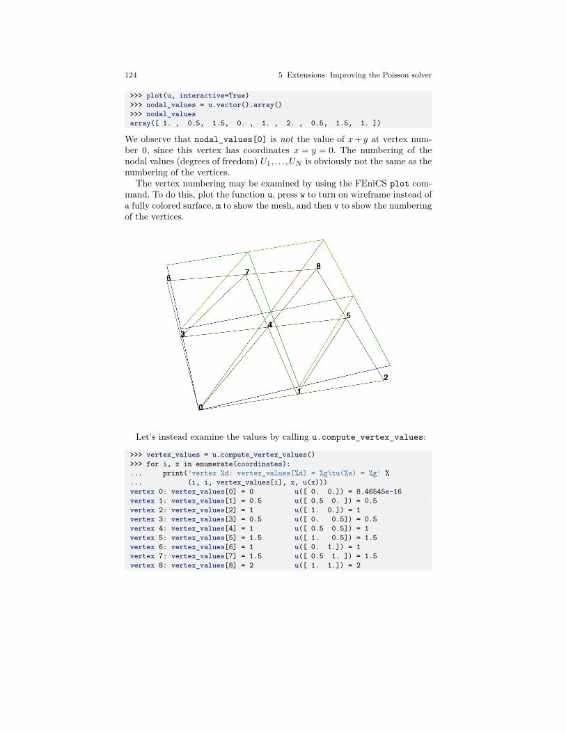
124 5 Extensions: Improving the Poisson solver
>>> plot(u, interactive=True)>>> nodal_values = u.vector().array()>>> nodal_valuesarray([ 1. , 0.5, 1.5, 0. , 1. , 2. , 0.5, 1.5, 1. ])
We observe that nodal_values[0] is not the value of x+ y at vertex num-ber 0, since this vertex has coordinates x = y = 0. The numbering of thenodal values (degrees of freedom) U1, . . . ,UN is obviously not the same as thenumbering of the vertices.
The vertex numbering may be examined by using the FEniCS plot com-mand. To do this, plot the function u, press w to turn on wireframe instead ofa fully colored surface, m to show the mesh, and then v to show the numberingof the vertices.
Let’s instead examine the values by calling u.compute_vertex_values:
>>> vertex_values = u.compute_vertex_values()>>> for i, x in enumerate(coordinates):... print(’vertex %d: vertex_values[%d] = %g\tu(%s) = %g’ %... (i, i, vertex_values[i], x, u(x)))vertex 0: vertex_values[0] = 0 u([ 0. 0.]) = 8.46545e-16vertex 1: vertex_values[1] = 0.5 u([ 0.5 0. ]) = 0.5vertex 2: vertex_values[2] = 1 u([ 1. 0.]) = 1vertex 3: vertex_values[3] = 0.5 u([ 0. 0.5]) = 0.5vertex 4: vertex_values[4] = 1 u([ 0.5 0.5]) = 1vertex 5: vertex_values[5] = 1.5 u([ 1. 0.5]) = 1.5vertex 6: vertex_values[6] = 1 u([ 0. 1.]) = 1vertex 7: vertex_values[7] = 1.5 u([ 0.5 1. ]) = 1.5vertex 8: vertex_values[8] = 2 u([ 1. 1.]) = 2
5.4 Degrees of freedom and function evaluation 125
We can ask FEniCS to give us the mapping from vertices to degrees offreedom for a certain function space V :
v2d = vertex_to_dof_map(V)
Now, nodal_values[v2d[i]] will give us the value of the degree of free-dom corresponding to vertex i (v2d[i]). In particular, nodal_values[v2d]is an array with all the elements in the same (vertex numbered) order ascoordinates. The inverse map, from degrees of freedom number to vertexnumber is given by dof_to_vertex_map(V). This means that we may callcoordinates[dof_to_vertex_map(V)] to get an array of all the coordinatesin the same order as the degrees of freedom. Note that these mappings areonly available in FEniCS for P1 elements.
For Lagrange elements of degree larger than 1, there are degrees of free-dom (nodes) that do not correspond to vertices. For these elements, we mayget the vertex values by calling u.compute_vertex_values(mesh), and wecan get the degrees of freedom by the call u.vector().array(). To get thecoordinates associated with all degrees of freedom, we need to iterate overthe elements of the mesh and ask FEniCS to return the coordinates anddofs associated with each element (cell). This information is stored in theFiniteElement and DofMap object of a FunctionSpace. The following codeillustrates how to iterate over all elements of a mesh and print the coordinatesand degrees of freedom associated with the element.
element = V.element()dofmap = V.dofmap()for cell in cells(mesh):
print(element.tabulate_dof_coordinates(cell))print(dofmap.cell_dofs(cell.index()))
5.4.2 Setting the degrees of freedom
We have seen how to extract the nodal values in a numpy array. If desired,we can adjust the nodal values too. Say we want to normalize the solutionsuch that maxj |Uj |= 1. Then we must divide all Uj values by maxj |Uj |. Thefollowing function performs the task:
def normalize_solution(u):"Normalize u: return u divided by max(u)"u_array = u.vector().array()u_max = np.max(np.abs(u_array))u_array /= u_maxu.vector()[:] = u_array#u.vector().set_local(u_array) # alternativereturn u
126 5 Extensions: Improving the Poisson solver
When using Lagrange elements, this (approximately) ensures that the maxi-mum value of the function u is 1.
The /= operator implies an in-place modification of the object on the left-hand side: all elements of the array nodal_values are divided by the valueu_max. Alternatively, we could do nodal_values = nodal_values / u_max,which implies creating a new array on the right-hand side and assigning thisarray to the name nodal_values.
Be careful when manipulating degrees of freedom
A call like u.vector().array() returns a copy of the data in u.vector().One must therefore never perform assignments like u.vector.array()[:]= ..., but instead extract the numpy array (i.e., a copy), manipulate it,and insert it back with u.vector()[:] = or use u.set_local(...).
5.4.3 Function evaluation
A FEniCS Function object is uniquely defined in the interior of each cellof the finite element mesh. For continuous (Lagrange) function spaces, thefunction values are also uniquely defined on cell boundaries. A Functionobject u can be evaluated by simply calling
u(x)
where x is either a Point or a Python tuple of the correct space dimension.When a Function is evaluated, FEniCS must first find which cell of the meshthat contains the given point (if any), and then evaluate a linear combinationof basis functions at the given point inside the cell in question. FEniCS usesefficient data structures (bounding box trees) to quickly find the point, butbuilding the tree is a relatively expensive operation so the cost of evaluatinga Function at a single point is costly. Repeated evaluation will reuse thecomputed data structures and thus be relatively less expensive.
Cheap vs expensive function evaluation
A Function object u can be evaluated in various ways:
1. u(x) for an arbitrary point x2. u.vector().array()[i] for degree of freedom number i3. u.compute_vertex_values()[i] at vertex number i
The first method, though very flexible, is in general expensive while theother two are very efficient (but limited to certain points).

5.5 Postprocessing computations 127
To demonstrate the use of point evaluation of Function objects, we printthe value of the computed finite element solution u for the Poisson problemat the center point of the domain and compare it with the exact solution:
center = (0.5, 0.5)error = u_D(center) - u(center)print(’Error at %s: %g’ % (center, error))
For a 2× (3×3) mesh, the output from the previous snippet becomes
Error at (0.5, 0.5): -0.0833333
The discrepancy is due to the fact that the center point is not a node in thisparticular mesh, but a point in the interior of a cell, and u varies linearly overthe cell while u_D is a quadratic function. When the center point is a node,as in a 2× (2×2) or 2× (4×4) mesh, the error is of the order 10−15.
5.5 Postprocessing computations
As the final theme in this chapter, we will look at how to postprocess computa-tions; that is, how to compute various derived quantities from the computedsolution of a PDE. The solution u itself may be of interest for visualizing gen-eral features of the solution, but sometimes one is interested in computingthe solution of a PDE to compute a specific quantity that derives from thesolution, such as, e.g., the flux, a point-value, or some average of the solution.
5.5.1 Test problem
As a test problem, we consider again the variable-coefficient Poisson problemwith a single Dirichlet boundary condition:
−∇· (κ∇u) = f in Ω, (5.1)u= uD on ∂Ω . (5.2)
Let us continue to use our favorite solution u(x,y) = 1 +x2 + 2y2 and thenprescribe κ(x,y) = x+y. It follows that uD(x,y) = 1+x2 +2y2 and f(x,y) =−8x−10y.
As before, the variational formulation for this model problem can be spec-ified in FEniCS as
a = kappa*dot(grad(u), grad(v))*dxL = f*v*dx
with the coefficient κ and right-hand side f given by
128 5 Extensions: Improving the Poisson solver
kappa = Expression(’x[0] + x[1]’, degree=1)f = Expression(’-8*x[0] - 10*x[1]’, degree=1)
5.5.2 Flux computations
It is often of interest to compute the flux Q=−κ∇u. Since u=∑Nj=1Ujφj ,
it follows that
Q=−κN∑j=1
Uj∇φj .
We note that the gradient of a piecewise continuous finite element scalar fieldis a discontinuous vector field since the basis functions φj have discontin-uous derivatives at the boundaries of the cells. For example, using Lagrangeelements of degree 1, u is linear over each cell, and the gradient becomes apiecewise constant vector field. On the contrary, the exact gradient is con-tinuous. For visualization and data analysis purposes, we often want thecomputed gradient to be a continuous vector field. Typically, we want eachcomponent of ∇u to be represented in the same way as u itself. To this end,we can project the components of ∇u onto the same function space as weused for u. This means that we solve w =∇u approximately by a finite ele-ment method, using the same elements for the components of w as we usedfor u. This process is known as projection.
Projection is a common operation in finite element analysis and, as we havealready seen, FEniCS has a function for easily performing the projection:project(expression, W), which returns the projection of some expressioninto the space W.
In our case, the flux Q=−κ∇u is vector-valued and we need to pick W asthe vector-valued function space of the same degree as the space V where uresides:
V = u.function_space()mesh = V.mesh()degree = V.ufl_element().degree()W = VectorFunctionSpace(mesh, ’P’, degree)
grad_u = project(grad(u), W)flux_u = project(-k*grad(u), W)
The applications of projection are many, including turning discontinuousgradient fields into continuous ones, comparing higher- and lower-order func-tion approximations, and transforming a higher-order finite element solutiondown to a piecewise linear field, which is required by many visualizationpackages.
Plotting the flux vector field is naturally as easy as plotting anything else:
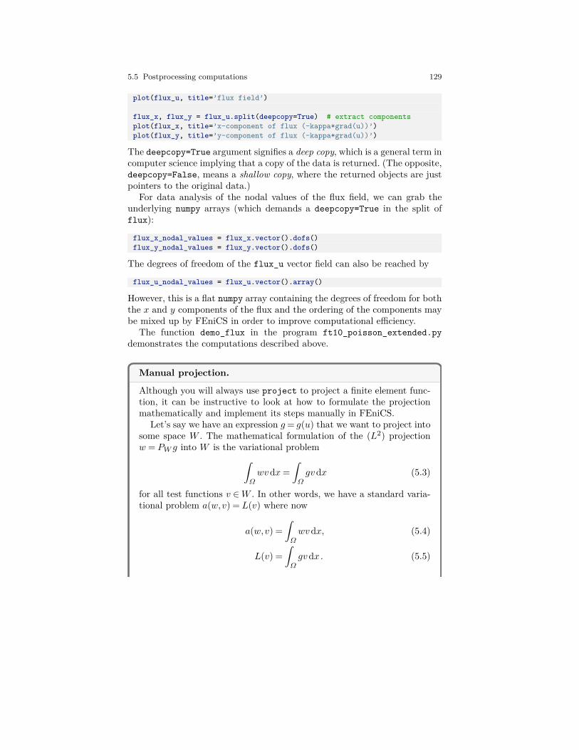
5.5 Postprocessing computations 129
plot(flux_u, title=’flux field’)
flux_x, flux_y = flux_u.split(deepcopy=True) # extract componentsplot(flux_x, title=’x-component of flux (-kappa*grad(u))’)plot(flux_y, title=’y-component of flux (-kappa*grad(u))’)
The deepcopy=True argument signifies a deep copy, which is a general term incomputer science implying that a copy of the data is returned. (The opposite,deepcopy=False, means a shallow copy, where the returned objects are justpointers to the original data.)
For data analysis of the nodal values of the flux field, we can grab theunderlying numpy arrays (which demands a deepcopy=True in the split offlux):
flux_x_nodal_values = flux_x.vector().dofs()flux_y_nodal_values = flux_y.vector().dofs()
The degrees of freedom of the flux_u vector field can also be reached by
flux_u_nodal_values = flux_u.vector().array()
However, this is a flat numpy array containing the degrees of freedom for boththe x and y components of the flux and the ordering of the components maybe mixed up by FEniCS in order to improve computational efficiency.
The function demo_flux in the program ft10_poisson_extended.pydemonstrates the computations described above.
Manual projection.
Although you will always use project to project a finite element func-tion, it can be instructive to look at how to formulate the projectionmathematically and implement its steps manually in FEniCS.
Let’s say we have an expression g= g(u) that we want to project intosome space W . The mathematical formulation of the (L2) projectionw = PW g into W is the variational problem∫
Ωwvdx=
∫Ωgvdx (5.3)
for all test functions v ∈W . In other words, we have a standard varia-tional problem a(w,v) = L(v) where now
a(w,v) =∫Ωwvdx, (5.4)
L(v) =∫Ωgvdx. (5.5)

130 5 Extensions: Improving the Poisson solver
Note that when the functions in W are vector-valued, as is the casewhen we project the gradient g(u) =∇u, we must replace the productsabove by w ·v and g ·v.
The variational problem is easy to define in FEniCS.
w = TrialFunction(W)v = TestFunction(W)
a = w*v*dx # or dot(w, v)*dx when w is vector-valuedL = g*v*dx # or dot(g, v)*dx when g is vector-valuedw = Function(W)solve(a == L, w)
The boundary condition argument to solve is dropped since there areno essential boundary conditions in this problem.
5.5.3 Computing functionals
After the solution u of a PDE is computed, we occasionally want to computefunctionals of u, for example,
12 ||∇u||
2 = 12
∫Ω∇u ·∇udx, (5.6)
which often reflects some energy quantity. Another frequently occurring func-tional is the error
||ue−u||=(∫
Ω(ue−u)2 dx
)1/2, (5.7)
where ue is the exact solution. The error is of particular interest when study-ing convergence properties of finite element methods. Other times, we mayinstead be interested in computing the flux out through a part Γ of theboundary ∂Ω,
F =−∫Γκ∇u ·nds, (5.8)
where n is the outward-pointing unit normal on Γ .All these functionals are easy to compute with FEniCS, as we shall see in
the examples below.
Energy functional. The integrand of the energy functional (5.6) is de-scribed in the UFL language in the same manner as we describe weak forms:
energy = 0.5*dot(grad(u), grad(u))*dxE = assemble(energy)

5.5 Postprocessing computations 131
The functional energy is evaluated by calling the assemble function that wehave previously used to assemble matrices and vectors. FEniCS will recognizethat the form has ”rank 0” (since it contains no trial and test functions) andreturn the result as a scalar value.
Error functional. The functional (5.7) can be computed as follows:
error = (u_e - u)**2*dxE = sqrt(abs(assemble(error)))
The exact solution ue is here represented by a Function or Expressionobject u_e, while u is the finite element approximation (and thus a Function).Sometimes, for very small error values, the result of assemble(error) canbe a (very small) negative number, so we have used abs in the expression forE above to ensure a positive value for the sqrt function.
As will be explained and demonstrated in Section 5.5.4, the integration of(u_e - u)**2*dx can result in too optimistic convergence rates unless one iscareful how the difference u_e - u is evaluated. The general recommendationfor reliable error computation is to use the errornorm function:
E = errornorm(u_e, u)
Flux Functional. To compute flux integrals like F = −∫Γ κ∇u ·nds, we
need to define the n vector, referred to as a facet normal in FEniCS. Ifthe surface domain Γ in the flux integral is the complete boundary, we canperform the flux computation by
n = FacetNormal(mesh)flux = -k*dot(grad(u), n)*dstotal_flux = assemble(flux)
Although grad(u) and nabla_grad(u) are interchangeable in the aboveexpression when u is a scalar function, we have chosen to write grad(u)because this is the right expression if we generalize the underlying equa-tion to a vector PDE. With nabla_grad(u) we must in that case writedot(n, nabla_grad(u)).
It is possible to restrict the integration to a part of the boundary by using amesh function to mark the relevant part, as explained in Section 4.4. Assum-ing that the part corresponds to subdomain number i, the relevant syntaxfor the variational formulation of the flux is -k*dot(grad(u), n)*ds(i).
A note on the accuracy of integration
As we have seen before, FEniCS Expressions must be defined usinga particular degree. The degree tells FEniCS into which local finiteelement space the expression should be interpolated when performinglocal computations (integration). As an illustration, consider the com-

132 5 Extensions: Improving the Poisson solver
putation of the integral∫ 1
0 cosxdx = sin1. This may be computed inFEniCS by
mesh = UnitIntervalMesh(1)I = assemble(Expression(’cos(x[0])’, degree=degree)*dx(domain=mesh))
Note that we must here specify the argument domain=mesh to the mea-sure dx. This is normally not necessary when defining forms in FEniCSbut is necessary here since cos(x[0]) is not associated with any domain(as is the case when we integrate a Function from some FunctionSpacedefined on some Mesh).
Varying the degree between 0 and 5, the value of |sin(1)−I| is 0.036,0.071, 0.00030, 0.00013, 4.5E-07, and 2.5E-07.
FEniCS also allows expressions to be expressed directly as part of aform. This requires the creation of a SpatialCoordinate. In this case,the accuracy is dictated by the accuracy of the integration, which maybe controlled by a degree argument to the integration measure dx.The degree argument specifies that the integration should be exact forpolynomials of that degree.
The following code snippet shows how to compute the integral∫ 10 cosxdx using this approach:
mesh = UnitIntervalMesh(1)x = SpatialCoordinate(mesh)I = assemble(cos(x[0])*dx(degree=degree))
Varying the degree between 0 and 5, the value of |sin(1)− I| is 0.036,0.036, 0.00020, 0.00020, 4.3E-07, 4.3E-07. Note that the quadraturedegrees are only available for odd degrees so that degree 0 will use thesame quadrature rule as degree 1, degree 2 will give the same quadraturerule as degree 3 and so on.
5.5.4 Computing convergence rates
A central question for any numerical method is its convergence rate: howfast does the error approach zero when the resolution is increased? For finiteelement methods, this typically corresponds to proving, theoretically or em-pirically, that the error e = ue−u is bounded by the mesh size h to somepower r; that is, ‖e‖ ≤ Chr for some constant C. The number r is called theconvergence rate of the method. Note that different norms, like the L2-norm‖e‖ or H1
0 -norm ‖∇e‖ typically have different convergence rates.To illustrate how to compute errors and convergence rates in FEniCS,
we have included the function compute_convergence_rates in the tutorialprogram ft10_poisson_extended.py. This is a tool that is very handy whenverifying finite element codes and will therefore be explained in detail here.
5.5 Postprocessing computations 133
Computing error norms. As we have already seen, the L2-norm of theerror ue−u can be implemented in FEniCS by
error = (u_e - u)**2*dxE = sqrt(abs(assemble(error)))
As above, we have used abs in the expression for E above to ensure a positivevalue for the sqrt function.
It is important to understand how FEniCS computes the error from theabove code, since we may otherwise run into subtle issues when using thevalue for computing convergence rates. The first subtle issue is that if u_e isnot already a finite element function (an object created using Function(V)),which is the case if u_e is defined as an Expression, FEniCS must interpolateu_e into some local finite element space on each element of the mesh. Thedegree used for the interpolation is determined by the mandatory keywordargument to the Expression class, for example:
u_e = Expression(’sin(x[0])’, degree=1)
This means that the error computed will not be equal to the actual error‖ue−u‖ but rather the difference between the finite element solution u andthe piecewise linear interpolant of ue. This may yield a too optimistic (toosmall) value for the error. A better value may be achieved by interpolatingthe exact solution into a higher-order function space, which can be done bysimply increasing the degree:
u_e = Expression(’sin(x[0])’, degree=3)
The second subtle issue is that when FEniCS evaluates the expression(u_e - u)**2, this will be expanded into u_e**2 + u**2 - 2*u_e*u. If theerror is small (and the solution itself is of moderate size), this calculationwill correspond to the subtraction of two positive numbers (u_e**2 + u**2∼ 1 and 2*u_e*u ∼ 1) yielding a small number. Such a computation is veryprone to round-off errors, which may again lead to an unreliable value for theerror. To make this situation worse, FEniCS may expand this computationinto a large number of terms, in particular for higher order elements, makingthe computation very unstable.
To help with these issues, FEniCS provides the built-in function errornormwhich computes the error norm in a more intelligent way. First, both u_e andu are interpolated into a higher-order function space. Then, the degrees offreedom of u_e and u are subtracted to produce a new function in the higher-order function space. Finally, FEniCS integrates the square of the differencefunction and then takes the square root to get the value of the error norm.Using the errornorm function is simple:
E = errornorm(u_e, u, normtype=’L2’)
It is illustrative to look at a short implementation of errornorm:
def errornorm(u_e, u):
134 5 Extensions: Improving the Poisson solver
V = u.function_space()mesh = V.mesh()degree = V.ufl_element().degree()W = FunctionSpace(mesh, ’P’, degree + 3)u_e_W = interpolate(u_e, W)u_W = interpolate(u, W)e_W = Function(W)e_W.vector()[:] = u_e_W.vector().array() - u_W.vector().array()error = e_W**2*dxreturn sqrt(abs(assemble(error)))
Sometimes it is of interest to compute the error of the gradient field:||∇(ue − u)||, often referred to as the H1
0 or H1 seminorm of the error.This can either be expressed as above, replacing the expression for errorby error = dot(grad(e_W), grad(e_W))*dx, or by calling errornorm inFEniCS:
E = errornorm(u_e, u, norm_type=’H10’)
Type help(errornorm) in Python for more information about available normtypes.
The function compute_errors in ft10_poisson_extended.py illustratesthe computation of various error norms in FEniCS.
Computing convergence rates. Let’s examine how to compute conver-gence rates in FEniCS. The solver function in ft10_poisson_extended.pyallows us to easily compute solutions for finer and finer meshes and enablesus to study the convergence rate. Define the element size h = 1/n, where nis the number of cell divisions in the x and y directions (n = Nx = Ny inthe code). We perform experiments with h0 > h1 > h2 > · · · and computethe corresponding errors E0,E1,E2 and so forth. Assuming Ei = Chri forunknown constants C and r, we can compare two consecutive experiments,Ei−1 = Chri−1 and Ei = Chri , and solve for r:
r = ln(Ei/Ei−1)ln(hi/hi−1) .
The r values should approach the expected convergence rate (typically thepolynomial degree + 1 for the L2-error) as i increases.
The procedure above can easily be turned into Python code. Here we runthrough a list of element degrees (P1, P2, and P3), perform experiments overa series of refined meshes, and for each experiment report the six error typesas returned by compute_errors.
Test problem. To demonstrate the computation of convergence rates, wepick an exact solution ue, this time a little more interesting than for the testproblem in Chapter 2:
ue(x,y) = sin(ωπx)sin(ωπy).
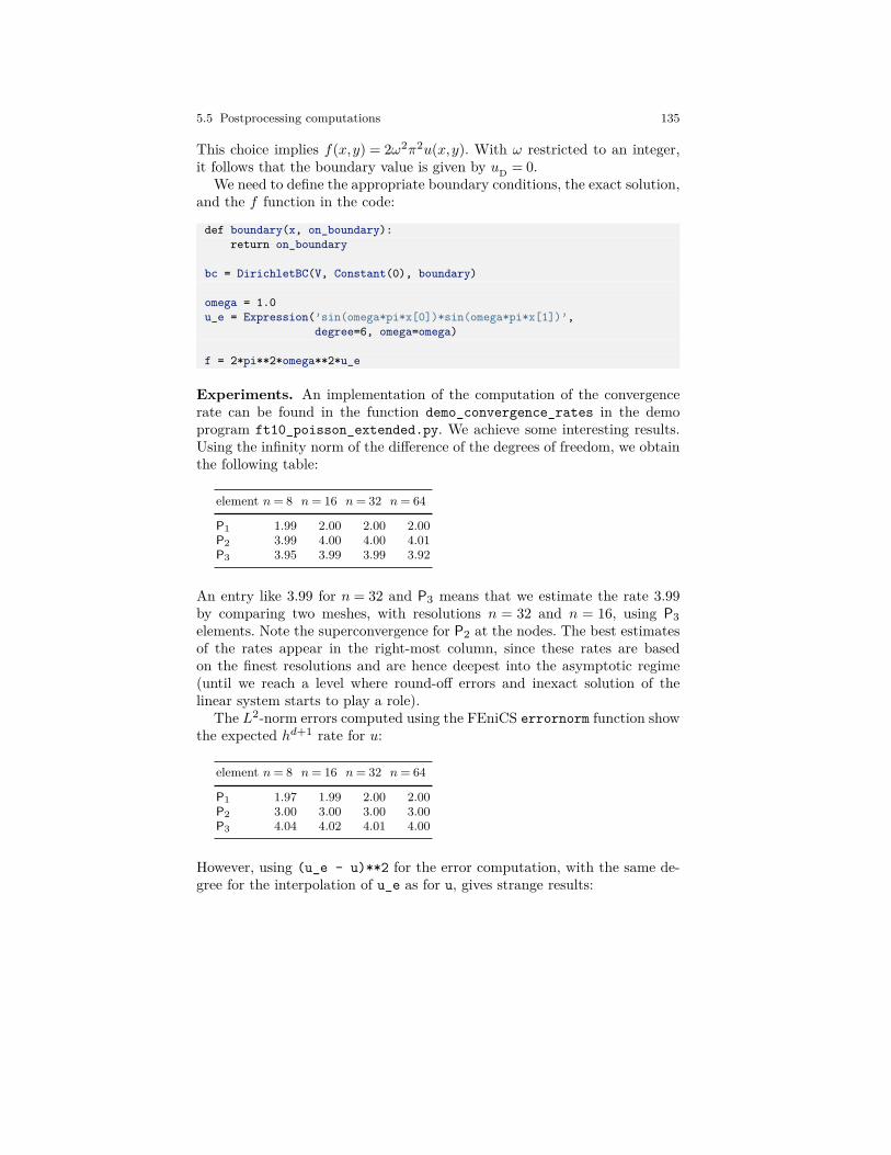
5.5 Postprocessing computations 135
This choice implies f(x,y) = 2ω2π2u(x,y). With ω restricted to an integer,it follows that the boundary value is given by uD = 0.
We need to define the appropriate boundary conditions, the exact solution,and the f function in the code:
def boundary(x, on_boundary):return on_boundary
bc = DirichletBC(V, Constant(0), boundary)
omega = 1.0u_e = Expression(’sin(omega*pi*x[0])*sin(omega*pi*x[1])’,
degree=6, omega=omega)
f = 2*pi**2*omega**2*u_e
Experiments. An implementation of the computation of the convergencerate can be found in the function demo_convergence_rates in the demoprogram ft10_poisson_extended.py. We achieve some interesting results.Using the infinity norm of the difference of the degrees of freedom, we obtainthe following table:
element n = 8 n = 16 n = 32 n = 64
P1 1.99 2.00 2.00 2.00P2 3.99 4.00 4.00 4.01P3 3.95 3.99 3.99 3.92
An entry like 3.99 for n = 32 and P3 means that we estimate the rate 3.99by comparing two meshes, with resolutions n = 32 and n = 16, using P3elements. Note the superconvergence for P2 at the nodes. The best estimatesof the rates appear in the right-most column, since these rates are basedon the finest resolutions and are hence deepest into the asymptotic regime(until we reach a level where round-off errors and inexact solution of thelinear system starts to play a role).
The L2-norm errors computed using the FEniCS errornorm function showthe expected hd+1 rate for u:
element n = 8 n = 16 n = 32 n = 64
P1 1.97 1.99 2.00 2.00P2 3.00 3.00 3.00 3.00P3 4.04 4.02 4.01 4.00
However, using (u_e - u)**2 for the error computation, with the same de-gree for the interpolation of u_e as for u, gives strange results:

136 5 Extensions: Improving the Poisson solver
element n = 8 n = 16 n = 32 n = 64
P1 1.97 1.99 2.00 2.00P2 3.00 3.00 3.00 3.01P3 4.04 4.07 1.91 0.00
This is an example where it is important to interpolate u_e to a higher-order space (polynomials of degree 3 are sufficient here). This is handledautomatically by using the errornorm function.
Checking convergence rates is an excellent method for verifying PDEcodes.
5.5.5 Taking advantage of structured mesh data
Many readers have extensive experience with visualization and data analysisof 1D, 2D, and 3D scalar and vector fields on uniform, structured meshes,while FEniCS solvers exclusively work with unstructured meshes. Since itcan many times be practical to work with structured data, we discuss in thissection how to extract structured data for finite element solutions computedwith FEniCS.
A necessary first step is to transform our Mesh object to an object repre-senting a rectangle (or a 3D box) with equally-shaped rectangular cells. Thesecond step is to transform the one-dimensional array of nodal values to atwo-dimensional array holding the values at the corners of the cells in thestructured mesh. We want to access a value by its i and j indices, i countingcells in the x direction, and j counting cells in the y direction. This trans-formation is in principle straightforward, yet it frequently leads to obscureindexing errors, so using software tools to ease the work is advantageous.
In the directory of example programs included with this book, we haveincluded the Python module boxfield which provides utilities for workingwith structured mesh data in FEniCS. Given a finite element function u, thefollowing function returns a BoxField object that represents u on a structuredmesh:
from boxfield import *u_box = FEniCSBoxField(u, (nx, ny))
The u_box object contains several useful data structures:
• u_box.grid: object for the structured mesh• u_box.grid.coor[X]: grid coordinates in X=0 direction• u_box.grid.coor[Y]: grid coordinates in Y=1 direction• u_box.grid.coor[Z]: grid coordinates in Z=2 direction• u_box.grid.coorv[X]: vectorized version of u_box.grid.coor[X]• u_box.grid.coorv[Y]: vectorized version of u_box.grid.coor[Y]
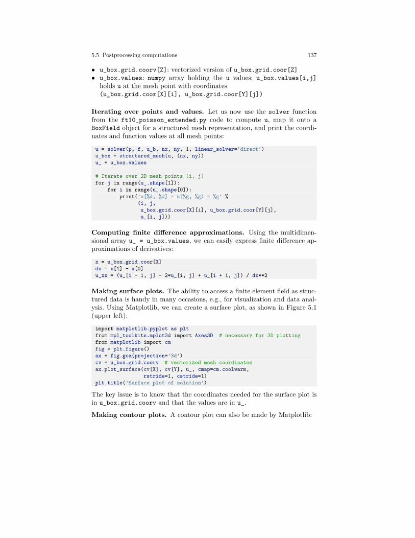
5.5 Postprocessing computations 137
• u_box.grid.coorv[Z]: vectorized version of u_box.grid.coor[Z]• u_box.values: numpy array holding the u values; u_box.values[i,j]
holds u at the mesh point with coordinates(u_box.grid.coor[X][i], u_box.grid.coor[Y][j])
Iterating over points and values. Let us now use the solver functionfrom the ft10_poisson_extended.py code to compute u, map it onto aBoxField object for a structured mesh representation, and print the coordi-nates and function values at all mesh points:
u = solver(p, f, u_b, nx, ny, 1, linear_solver=’direct’)u_box = structured_mesh(u, (nx, ny))u_ = u_box.values
# Iterate over 2D mesh points (i, j)for j in range(u_.shape[1]):
for i in range(u_.shape[0]):print(’u[%d, %d] = u(%g, %g) = %g’ %
(i, j,u_box.grid.coor[X][i], u_box.grid.coor[Y][j],u_[i, j]))
Computing finite difference approximations. Using the multidimen-sional array u_ = u_box.values, we can easily express finite difference ap-proximations of derivatives:
x = u_box.grid.coor[X]dx = x[1] - x[0]u_xx = (u_[i - 1, j] - 2*u_[i, j] + u_[i + 1, j]) / dx**2
Making surface plots. The ability to access a finite element field as struc-tured data is handy in many occasions, e.g., for visualization and data anal-ysis. Using Matplotlib, we can create a surface plot, as shown in Figure 5.1(upper left):
import matplotlib.pyplot as pltfrom mpl_toolkits.mplot3d import Axes3D # necessary for 3D plottingfrom matplotlib import cmfig = plt.figure()ax = fig.gca(projection=’3d’)cv = u_box.grid.coorv # vectorized mesh coordinatesax.plot_surface(cv[X], cv[Y], u_, cmap=cm.coolwarm,
rstride=1, cstride=1)plt.title(’Surface plot of solution’)
The key issue is to know that the coordinates needed for the surface plot isin u_box.grid.coorv and that the values are in u_.
Making contour plots. A contour plot can also be made by Matplotlib:

138 5 Extensions: Improving the Poisson solver
0.00.2
0.40.6
0.81.0 0.0
0.20.4
0.60.8
1.00.40.2
0.00.20.40.60.8
1.0
Surface plot of solution
0.0 0.2 0.4 0.6 0.8 1.00.0
0.2
0.4
0.6
0.8
1.0
0.000
0.00
0
0.000
0.20
00.
400
0.60
00.
800
Contour plot of solution
0.0 0.2 0.4 0.6 0.8 1.0x
0.2
0.1
0.0
0.1
0.2
0.3
0.4
0.5
0.6
u
Solution along line y=0.409091
P1 elementsexact
0.0 0.2 0.4 0.6 0.8 1.0x
6
4
2
0
2
4
6
u
Flux along line y=0.409091
P1 elementsexact
Fig. 5.1 Various plots of the solution on a structured mesh.
fig = plt.figure()ax = fig.gca()levels = [1.5, 2.0, 2.5, 3.5]cs = ax.contour(cv[X], cv[Y], u_, levels=levels)plt.clabel(cs) # add labels to contour linesplt.axis(’equal’)plt.title(’Contour plot of solution’)
The result appears in Figure 5.1 (upper right).
Making curve plots through the domain. A handy feature of BoxFieldobjects is the ability to give a starting point in the domain and a direction,and then extract the field and corresponding coordinates along the nearestline ofmesh points. We have already seen how to interpolate the solution alonga line in the mesh, but with BoxField you can pick out the computationalpoints (vertices) for examination of these points. Numerical methods oftenshow improved behavior at such points so this is of interest. For 3D fields onecan also extract data in a plane.
Say we want to plot u along the line y = 0.4. The mesh points, x, and theu values along this line, u_val, can be extracted by
start = (0, 0.4)x, u_val, y_fixed, snapped = u_box.gridline(start, direction=X)

5.5 Postprocessing computations 139
The variable snapped is true if the line is snapped onto to nearest gridlineand in that case y_fixed holds the snapped (altered) y value. The keywordargument snap is by default True to avoid interpolation and force snapping.
A comparison of the numerical and exact solution along the line y ≈ 0.41(snapped from y = 0.4) is made by the following code:
# Plot u along a line y = const and compare with exact solutionstart = (0, 0.4)x, u_val, y_fixed, snapped = u_box.gridline(start, direction=X)u_e_val = [u_D((x_, y_fixed)) for x_ in x]plt.figure()plt.plot(x, u_val, ’r-’)plt.plot(x, u_e_val, ’bo’)plt.legend([’P1 elements’, ’exact’], loc=’best’)plt.title(’Solution along line y=%g’ % y_fixed)plt.xlabel(’x’); plt.ylabel(’u’)
See Figure 5.1 (lower left) for the resulting curve plot.
Making curve plots of the flux. Let us also compare the numerical andexact fluxes −κ∂u/∂x along the same line as above:
# Plot the numerical and exact flux along the same lineflux_u = flux(u, kappa)flux_u_x, flux_u_y = flux_u.split(deepcopy=True)flux2_x = flux_u_x if flux_u_x.ufl_element().degree() == 1 \
else interpolate(flux_x,FunctionSpace(u.function_space().mesh(), ’P’, 1))
flux_u_x_box = FEniCSBoxField(flux_u_x, (nx,ny))x, flux_u_val, y_fixed, snapped = \
flux_u_x_box.gridline(start, direction=X)y = y_fixedplt.figure()plt.plot(x, flux_u_val, ’r-’)plt.plot(x, flux_u_x_exact(x, y_fixed), ’bo’)plt.legend([’P1 elements’, ’exact’], loc=’best’)plt.title(’Flux along line y=%g’ % y_fixed)plt.xlabel(’x’); plt.ylabel(’u’)
The function flux called at the beginning of the code snippet is defined inthe example program ft10_poisson_extended.py and interpolates the fluxback into the function space.
Note that Matplotlib is one choice of plotting package. With the unifiedinterface in the SciTools package1 one can access Matplotlib, Gnuplot, MAT-LAB, OpenDX, VisIt, and other plotting engines through the same API.
Test problem. The graphics referred to in Figure 5.1 correspond to a testproblem with prescribed solution ue =H(x)H(y), where
H(x) = e−16(x− 12 )2
sin(3πx) .
1https://github.com/hplgit/scitools
140 5 Extensions: Improving the Poisson solver
The corresponding right-hand side f is obtained by inserting the exact solu-tion into the PDE and differentiating as before. Although it is easy to carryout the differentiation of f by hand and hardcode the resulting expressionsin an Expression object, a more reliable habit is to use Python’s symboliccomputing engine, SymPy, to perform mathematics and automatically turnformulas into C++ syntax for Expression objects. A short introduction wasgiven in Section 3.2.3.
We start out with defining the exact solution in sympy:
from sympy import exp, sin, pi # for use in math formulasimport sympy as sym
H = lambda x: exp(-16*(x-0.5)**2)*sin(3*pi*x)x, y = sym.symbols(’x[0], x[1]’)u = H(x)*H(y)
Turning the expression for u into C or C++ syntax for Expression objectsneeds two steps. First we ask for the C code of the expression:
u_code = sym.printing.ccode(u)
Printing u_code gives (the output is here manually broken into two lines):
-exp(-16*pow(x[0] - 0.5, 2) - 16*pow(x[1] - 0.5, 2))*sin(3*M_PI*x[0])*sin(3*M_PI*x[1])
The necessary syntax adjustment is replacing the symbol M_PI for π inC/C++ by pi (or DOLFIN_PI):
u_code = u_code.replace(’M_PI’, ’pi’)u_b = Expression(u_code, degree=1)
Thereafter, we can progress with the computation of f =−∇· (κ∇u):
kappa = 1f = sym.diff(-kappa*sym.diff(u, x), x) + \
sym.diff(-kappa*sym.diff(u, y), y)f = sym.simplify(f)f_code = sym.printing.ccode(f)f_code = f_code.replace(’M_PI’, ’pi’)f = Expression(f_code, degree=1)
We also need a Python function for the exact flux −κ∂u/∂x:
flux_u_x_exact = sym.lambdify([x, y], -kappa*sym.diff(u, x),modules=’numpy’)
It remains to define kappa = Constant(1) and set nx and ny before callingsolver to compute the finite element solution of this problem.
5.6 Taking the next step 141
5.6 Taking the next step
If you have come this far, you have learned how to both write simple script-like solvers for a range of PDEs, and how to structure Python solvers usingfunctions and unit tests. Solving a more complex PDE and writing a morefull-featured PDE solver is not much harder and the first step is typically towrite a solver for a stripped-down test case as a simple Python script. As thescript matures and becomes more complex, it is time to think about design,in particular how to modularize the code and organize it into reusable piecesthat can be used to build a flexible and extensible solver.
On the FEniCS web site you will find more extensive documentation, moreexample programs, and links to advanced solvers and applications written ontop of FEniCS. Get inspired and develop your own solver for your favoriteapplication, publish your code and share your knowledge with the FEniCScommunity and the world!
PS: Stay tuned for the FEniCS Tutorial Volume 2!


References
[1] M. S. Alnæs, A. Logg, K. B. Ølgaard, M. E. Rognes, and G. N. Wells.Unified Form Language: A domain-specific language for weak formula-tions of partial differential equations. ACM Transactions on Mathemat-ical Software, 40(2), 2014. doi:10.1145/2566630, arXiv:1211.4047.
[2] Douglas N. Arnold and Anders Logg. Periodic table of the finite ele-ments. SIAM News, 2014.
[3] W. B. Bickford. A First Course in the Finite Element Method. Irwin,2nd edition, 1994.
[4] D. Braess. Finite Elements. Cambridge University Press, Cambridge,third edition, 2007.
[5] S. C. Brenner and L. R. Scott. The Mathematical Theory of FiniteElement Methods, volume 15 of Texts in Applied Mathematics. Springer,New York, third edition, 2008.
[6] A. J. Chorin. Numerical solution of the Navier-Stokes equations. Math.Comp., 22:745–762, 1968.
[7] P. G. Ciarlet. The Finite Element Method for Elliptic Problems, vol-ume 40 of Classics in Applied Mathematics. SIAM, Philadelphia,PA, 2002. Reprint of the 1978 original [North-Holland, Amsterdam;MR0520174 (58 #25001)].
[8] J. Donea and A. Huerta. Finite Element Methods for Flow Problems.Wiley Press, 2003.
[9] K. Eriksson, D. Estep, P. Hansbo, and C. Johnson. Computational Dif-ferential Equations. Cambridge University Press, 1996.
[10] A. Ern and J.-L. Guermond. Theory and Practice of Finite Elements.Springer, 2004.
[11] Python Software Foundation. The Python tutorial. http://docs.python.org/2/tutorial.
[12] M. Gockenbach. Understanding and Implementing the Finite ElementMethod. SIAM, 2006.
c© 2017, Hans Petter Langtangen, Anders Logg.Released under CC Attribution 4.0 license
144 REFERENCES
[13] K. Goda. A multistep technique with implicit difference schemes forcalculating two- or three-dimensional cavity flows. Journal of Computa-tional Physics, 30(1):76–95, 1979.
[14] T. J. R. Hughes. The Finite Element Method: Linear Static and DynamicFinite Element Analysis. Prentice-Hall, 1987.
[15] J. M. Kinder and P. Nelson. A Student’s Guide to Python for PhysicalModeling. Princeton University Press, 2015.
[16] Robert C. Kirby. Fiat, a new paradigm for computing finite element basisfunctions. ACM Transactions on Mathematical Software, 30(4):502–516,2004.
[17] Robert C. Kirby and Anders Logg. A compiler for variational forms.ACM Transactions on Mathematical Software, 32(3):417–444, 2006.
[18] J. Kiusalaas. Numerical Methods in Engineering With Python. Cam-bridge University Press, 2005.
[19] R. H. Landau, M. J. Paez, and C. C. Bordeianu. Computational Physics:Problem Solving with Python. Wiley, third edition, 2015.
[20] H. P. Langtangen. Python Scripting for Computational Science.Springer, third edition, 2009.
[21] H. P. Langtangen. A Primer on Scientific Programming With Python.Texts in Computational Science and Engineering. Springer, fifth edition,2016.
[22] H. P. Langtangen and L. R. Hellevik. Brief tutorials on scientific Python,2016. http://hplgit.github.io/bumpy/doc/web/index.html.
[23] H. P. Langtangen and A. Logg. Solving PDEs in Hours – The FEniCSTutorial Volume II. Springer, 2016.
[24] H. P. Langtangen and K.-A. Mardal. Introduction to Numerical Methodsfor Variational Problems. 2016. http://hplgit.github.io/fem-book/doc/web/.
[25] M. G. Larson and F. Bengzon. The Finite Element Method: Theory,Implementation, and Applications. Texts in Computational Science andEngineering. Springer, 2013.
[26] A. Logg, K.-A. Mardal, and G. N. Wells. Automated Solution of PartialDifferential Equations by the Finite Element Method. Springer, 2012.
[27] Anders Logg and Garth N. Wells. DOLFIN: Automated finite elementcomputing. ACM Transactions on Mathematical Software, 37(2), 2010.
[28] M. Pilgrim. Dive into Python. Apress, 2004. http://www.diveintopython.net.
[29] A. Quarteroni and A. Valli. Numerical Approximation of Partial Dif-ferential Equations. Springer Series in Computational Mathematics.Springer, 1994.
[30] A. Henderson Squillacote. The ParaView Guide. Kitware, 2007.[31] R. Temam. Sur l’approximation de la solution des équations de Navier-
Stokes. Arc. Ration. Mech. Anal., 32:377–385, 1969.
Index
.hdf5 file, 69
.pvd file, 45
.vtu file, 45
.xdmf file, 69
abstract variational formulation, 15advection–diffusion–reaction, 73assemble, 64, 119, 120assemble_system, 120assembly, 119
backward difference, 38boundary conditions, 92boundary markers, 88boundary specification (class), 88boundary specification (function), 21,
22BoxField, 136
C++ expression syntax, 22CellFunction, 88CFD, 56channel flow, 60chemical reactions, 73Chorin’s method, 57Circle, 102code, 8CompiledSubDomain, 91components, 81
constructive solid geometry, 67contour plot, 137convergence rate, 132coordinates, 123coupled systems, 73CSG, 67curve plots, 34cylinder flow, 65
Debian, 7DEBUG log level, 67deep copy, 81degrees of freedom, 25, 29, 30, 129degrees of freedrom, 123dimension-independent code, 114Dirichlet boundary condition, 92Dirichlet boundary conditions, 20DirichletBC, 20Docker, 6dof to vertex map, 124dofs, 29DOLFIN, 3
editor, 7Eigen, 115elasticity, 50Emacs, 7energy functional, 130error, 28, 133
145

146 INDEX
error functional, 131errornorm, 131exact solution, 16exporting solutions, 27Expression, 21, 32expression syntax (C++), 22
FacetFunction, 88fenicsproject, 6FFC, 3FIAT, 3finite element method, 9finite element space, 20flat program, 109flux functional, 131ft01_poisson.py, 18ft02_poisson_membrane.py, 34ft03_heat.py, 44ft04_heat_gaussian.py, 46ft05_poisson_nonlinear.py, 50ft06_elasticity.py, 54ft07_navier_stokes_channel.py, 65ft08_navier_stokes_cylinder.py, 73ft09_reaction_system.py, 80ft10_poisson_extended.py, 97, 117,
127ft11_magnetostatics.py, 107ft12_poisson_solver.py, 111function evaluation, 126function space, 20functionals, 130FunctionSpace, 20
generate_mesh, 67, 102GNU/Linux, 5grad, 58
HDF5 format, 69heat equation, 37heterogeneous media, 87
implicit Euler, 38incremental pressure correction scheme,
57infinite domain, 101info, 116
initial condition, 80installation, 5integration by parts, 13interpolate, 40interpolation, 41
Jacobian, 50Jupyter, 19
Krylov solver, 68, 115, 117KrylovSolver, 121
Lagrange finite element, 20lhs, 41, 97linear algebra backend, 115linear solver, 115, 117linear system, 64, 120LinearVariationalProblem, 118LinearVariationalSolver, 118Linux, 5
Mac OS X, 5magnetostatics, 100MATLAB, 122Maxwell’s equations, 100Measure, 104Mesh, 19mesh, 19mesh generation, 102MeshFunction, 88method of manufactured solutions, 16,
48mixed finite element, 76mixed function space, 76MixedElement, 76mshr, 3, 67, 102multi-material domain, 87
nabla_grad, 54, 58Navier-Stokes equations, 56near, 62, 85Neumann boundary condition, 83, 92Newton’s method, 50nodal values, 29, 30, 129nonlinear problem, 46norm, 133

INDEX 147
numberingcell vertices, 30degrees of freedom, 30
P1 element, 20packages, 7parameters, 116ParaView, 27performance, 6Periodic Table of the Finite Elements,
20PETSc, 3, 115plot, 25plotting, 25Poisson’s equation, 11postprocessing, 27, 127preconditioner, 68, 115, 117PROGRESS log level, 67Progress, 67project, 40, 128projection, 41Python, 8Python module, 111
reaction system, 73Reynolds number, 60rhs, 41, 97Robin boundary condition, 92rounding errors, 23
scaling, 55, 60scitools, 136set_log_level, 67SLEPc, 122source, 5space dimensions, 114split, 81splitting method, 57Spyder, 19strain-rate tensor, 57stress tensor, 51, 56structured mesh, 136subdomains, 83surface plot (structured mesh), 137SymPy, 48sympy, 139
system of PDEs, 50
tensor, 51terminal window, 18test function, 13test problem, 16TestFunction, 20time step, 38time-dependent expression, 41time-dependent problem, 37TimeSeries, 69, 76tolerance, 23trial function, 13TrialFunction, 20
Ubuntu, 7UFL, 3, 24unit testing, 111
variational formulation, 12vector-valued functions, 54VectorElement, 77VectorFunctionSpace, 54, 62verification, 16, 65, 111vertex to dof map, 124vertex values, 29, 123, 124Vim, 7visualization, structured mesh, 136VTK format, 45
Windows, 5
XDMF format, 69