Some implications of (non-)ergodicity of psychological processes

Spencer Conference

Chicago University

December 10-11, 2010

Peter Molenaar

The Pennsylvania State University

Email: pxm21@psu.edu

Standard approach to statistical analysis in psychology:

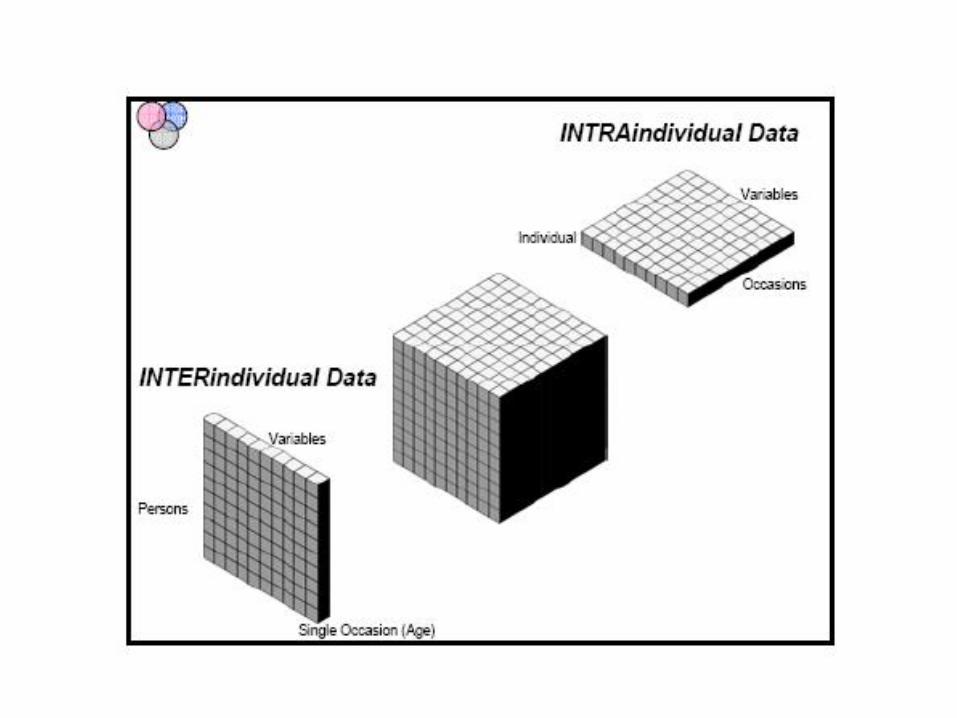
- Analysis of inter-individual variation (variation between subjects in a population of subjects; individual differences)

- Strong assumption of homogeneity in (sub-)populations

- Aimed at generalization to the state of affairs at the population level

- Implicit assumption of applicability of results at the individual level of intra-individual variation

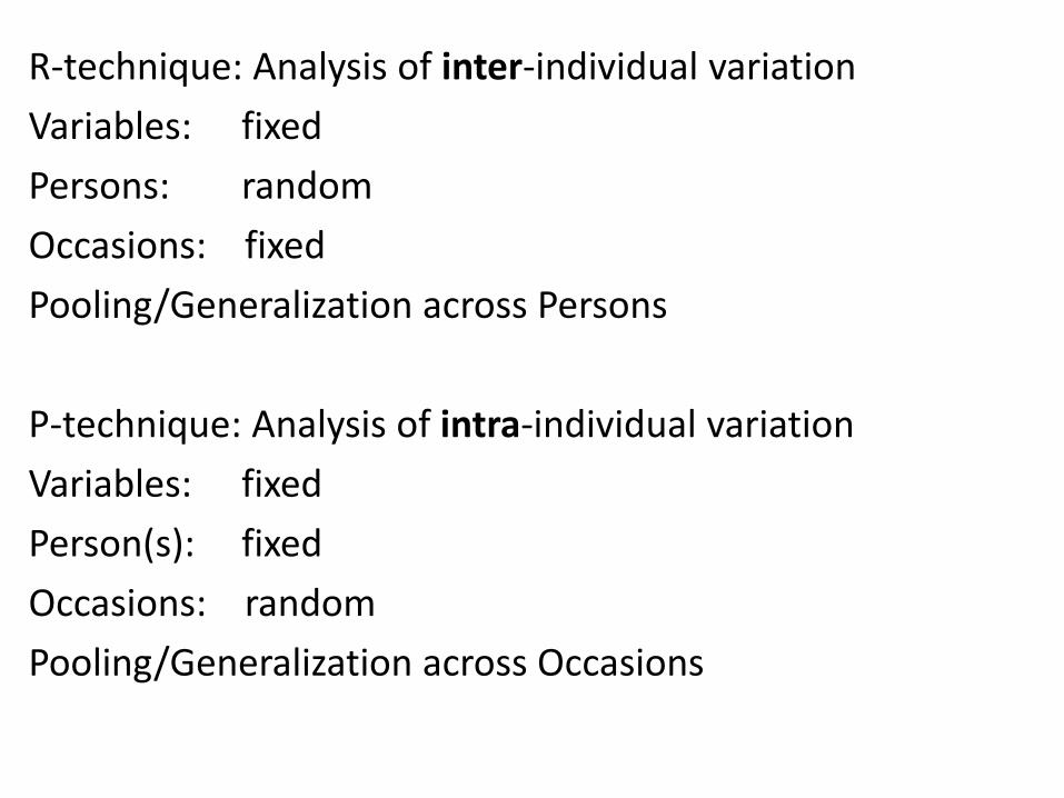
R-technique: Analysis of inter-individual variation

Variables: fixed

Persons: random

Occasions: fixed

Pooling/Generalization across Persons

P-technique: Analysis of intra-individual variation

Variables: fixed

Person(s): fixed

Occasions: random

Pooling/Generalization across Occasions

Basic Question:

Can results obtained in analyses of inter-individual variation be validly generalized to the subject-specific level of intra-individual variation (and vice versa)?

Molenaar, Measurement, 2004

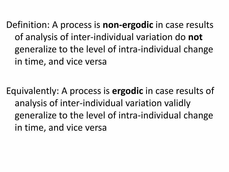
Definition: A process is non-ergodic in case results of analysis of inter-individual variation do notgeneralize to the level of intra-individual change in time, and vice versa

Equivalently: A process is ergodic in case results of analysis of inter-individual variation validly generalize to the level of intra-individual change in time, and vice versa

Ergodicity is not a generic property of homogeneous Hamiltonian systems (the primary class of candidate ergodic dynamic systems).

Ergodicity is the weakest property in the ergodichierarchy, including mixing and K-systems.

Emch, G., & Liu, C. (2002). The logic of thermo-statistical physics. Berlin: Springer.

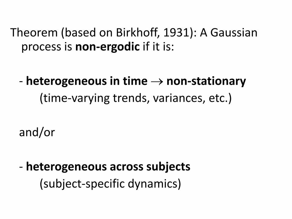
Theorem (based on Birkhoff, 1931): A Gaussian process is non-ergodic if it is:

- heterogeneous in time non-stationary

(time-varying trends, variances, etc.)

and/or

- heterogeneous across subjects

(subject-specific dynamics)

Model heterogeneity across subjects (second criterion in Theorem) is invisible in standard factor analysis of inter-individual variation.

Formal proof in: Kelderman & Molenaar (2007) Multivariate Behavioral Research, 42, 435-456.

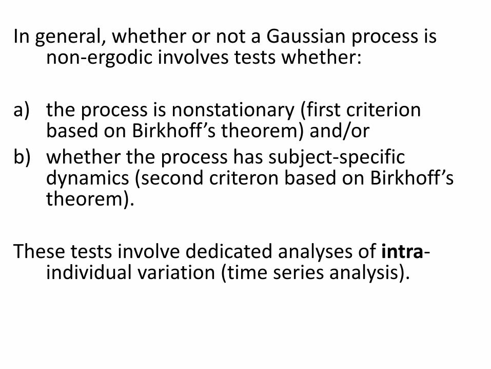
In general, whether or not a Gaussian process is non-ergodic involves tests whether:

a) the process is nonstationary (first criterion based on Birkhoff’s theorem) and/or

b) whether the process has subject-specific dynamics (second criteron based on Birkhoff’stheorem).

These tests involve dedicated analyses of intra-individual variation (time series analysis).

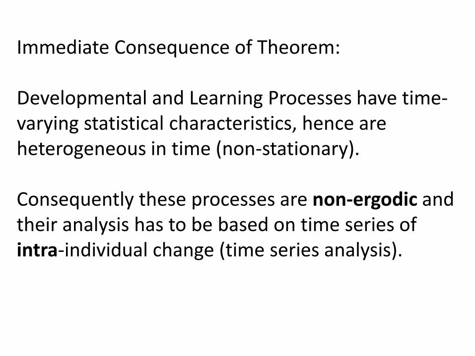
Immediate Consequence of Theorem:

Developmental and Learning Processes have time-varying statistical characteristics, hence are heterogeneous in time (non-stationary).

Consequently these processes are non-ergodic and their analysis has to be based on time series of intra-individual change (time series analysis).

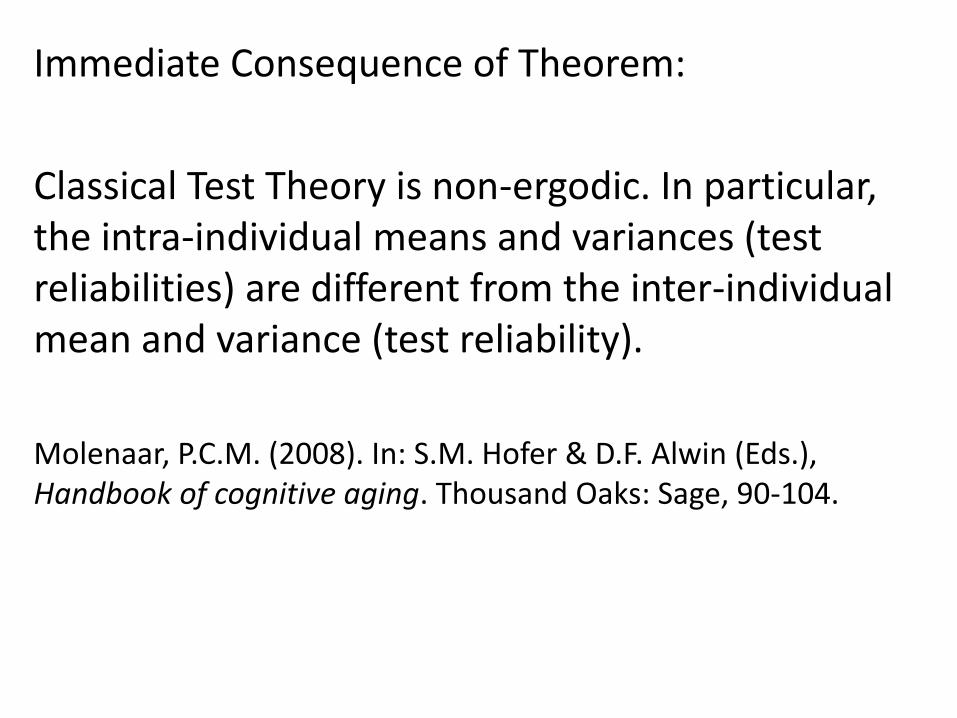
Immediate Consequence of Theorem:

Classical Test Theory is non-ergodic. In particular, the intra-individual means and variances (test reliabilities) are different from the inter-individual mean and variance (test reliability).

Molenaar, P.C.M. (2008). In: S.M. Hofer & D.F. Alwin (Eds.), Handbook of cognitive aging. Thousand Oaks: Sage, 90-104.

Testing heterogeneity across subjects (second criterion based on Birkhoff’s theorem)

Person-Specific Factor Models

Molenaar & Campbell, Current Directions in Psychology, 2009

Hamaker, Dolan, & Molenaar, Multivariate Behavioral Research, 2005

Timmerman, Dissertation, 2001

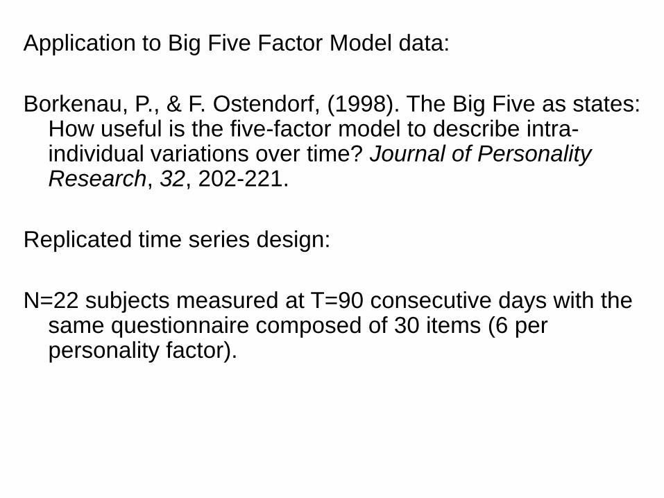
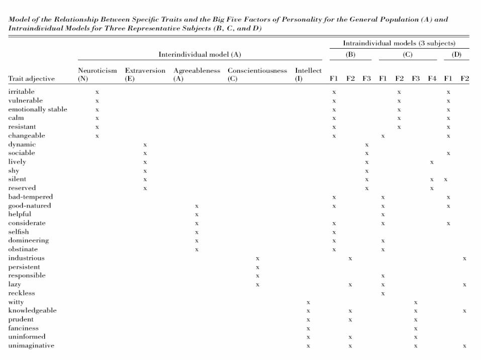
Application to Big Five Factor Model data:

Borkenau, P., & F. Ostendorf, (1998). The Big Five as states: How useful is the five-factor model to describe intra-individual variations over time? Journal of Personality Research, 32, 202-221.

Replicated time series design:

N=22 subjects measured at T=90 consecutive days with the same questionnaire composed of 30 items (6 per personality factor).

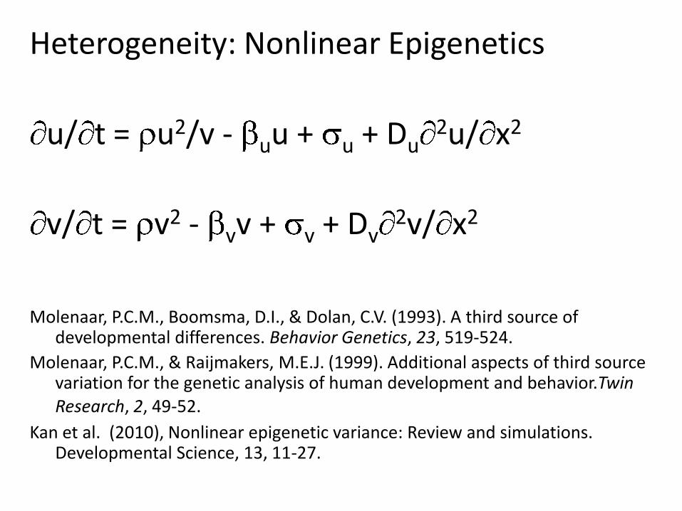
Heterogeneity: Nonlinear Epigenetics

u/ t = u2/v - uu + u + Du2u/ x2

v/ t = v2 - vv + v + Dv2v/ x2

Molenaar, P.C.M., Boomsma, D.I., & Dolan, C.V. (1993). A third source of developmental differences. Behavior Genetics, 23, 519-524.

Molenaar, P.C.M., & Raijmakers, M.E.J. (1999). Additional aspects of third source variation for the genetic analysis of human development and behavior.TwinResearch, 2, 49-52.

Kan et al. (2010), Nonlinear epigenetic variance: Review and simulations. Developmental Science, 13, 11-27.

Heterogeneity: Functional brain connectivity

The functional neural networks underlying brain processes differ dramatically across individuals throughout the life span and therefore their analysis should be based on intra-individual variation, not group data.

Nelson, C.A., de Haan, M., & Thomas, K.M. (2006). Neuroscience of cognitive

development: the role of experience and the developing brain. New York: Wiley.

Sporns, O. (2010). Networks of the brain. Cambridge, Mass.: MIT Press.

Heterogeneity: Human decision making

“Each axiom should be tested in as much isolation as possible, and it should be done in-so-far as possible for each person individually, not using group aggregations.”

Luce, R.D. (2000). Utility of gains and losses: Measurement-theoretical and experimental approaches. Mahwah, NJ, Erlbaum, p.29

“Extremely large individual differences” in binary choice behavior.

Erev, I., & Barron, G. (2005). On adaptation, maximization, and reinforcement learning among cognitive strategies. Psychological Review, 112, 912-931.

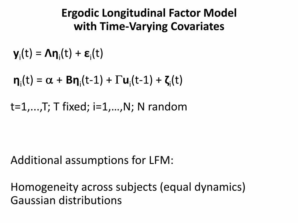
Ergodic Longitudinal Factor Model with Time-Varying Covariates

yi(t) = Ληi(t) + εi(t)

ηi(t) = + Bηi(t-1) + ui(t-1) + ζi(t)

t=1,...,T; T fixed; i=1,…,N; N random

Additional assumptions for LFM:

Homogeneity across subjects (equal dynamics)Gaussian distributions

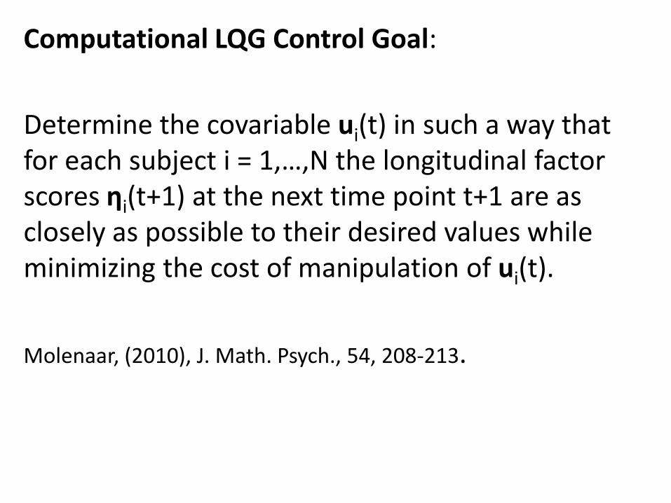
Computational LQG Control Goal:

Determine the covariable ui(t) in such a way that for each subject i = 1,…,N the longitudinal factor scores ηi(t+1) at the next time point t+1 are as closely as possible to their desired values while minimizing the cost of manipulation of ui(t).

Molenaar, (2010), J. Math. Psych., 54, 208-213.

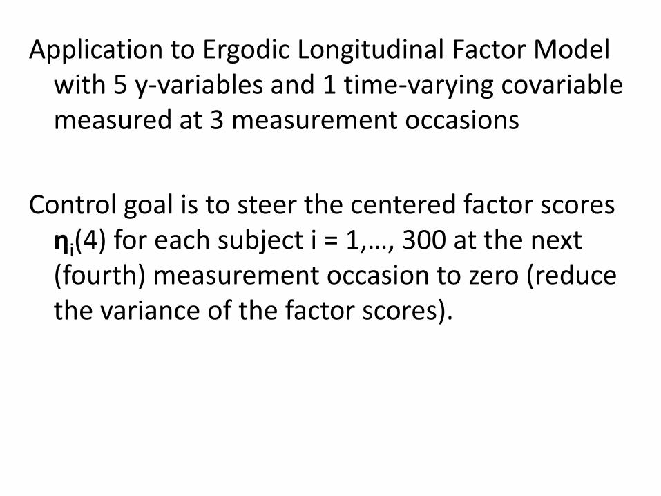
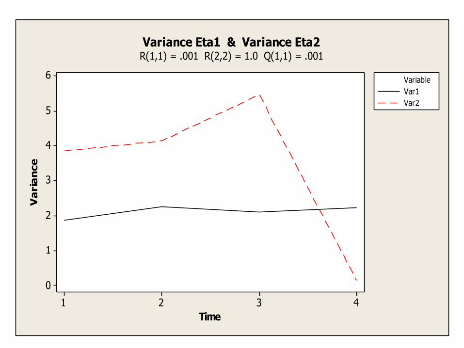
Application to Ergodic Longitudinal Factor Model with 5 y-variables and 1 time-varying covariablemeasured at 3 measurement occasions

Control goal is to steer the centered factor scores ηi(4) for each subject i = 1,…, 300 at the next(fourth) measurement occasion to zero (reducethe variance of the factor scores).

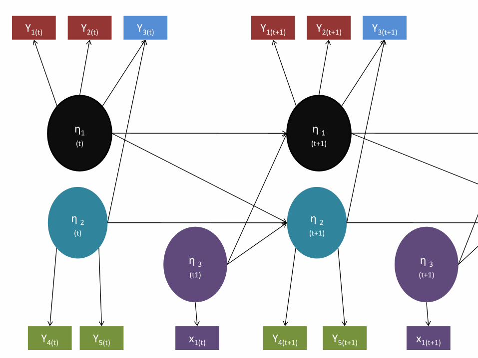
η1

(t)

η 2(t)

Y1(t) Y2(t)

Y4(t) x1(t)

Y3(t)

Y5(t)

η 3(t1)

η 1(t+1)

η 2(t+1)

Y1(t+1) Y2(t+1)

Y4(t+1)

Y3(t+1)

Y5(t+1) x1(t+1)

η 3(t+1)

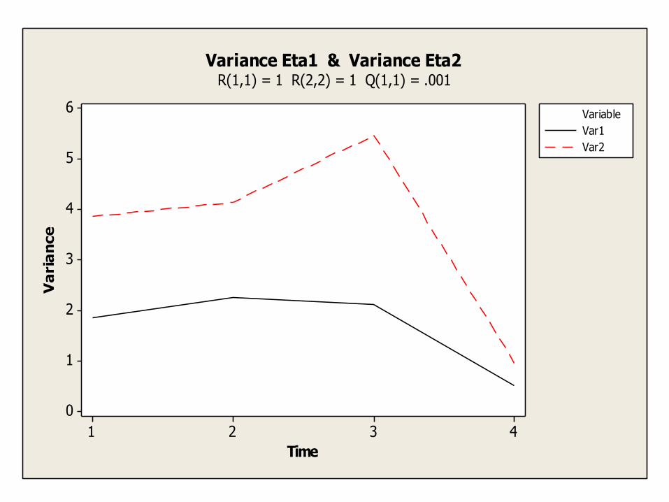
4321

6

5

4

3

2

1

0

Time

Va

ria

nce

Var1

Var2

Variable

Variance Eta1 & Variance Eta2R(1,1) = 1 R(2,2) = 1 Q(1,1) = .001

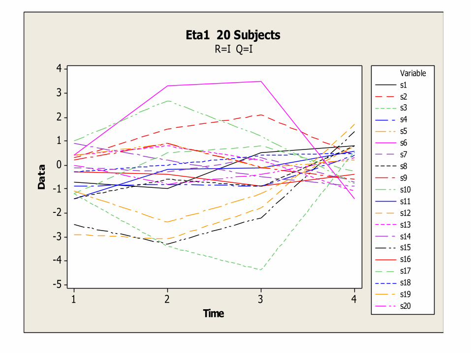
4321

4

3

2

1

0

-1

-2

-3

-4

-5

Time

Da

ta

s10

s11

s12

s13

s14

s15

s16

s17

s18

s19

s1

s20

s2

s3

s4

s5

s6

s7

s8

s9

Variable

Eta1 20 SubjectsR=I Q=I

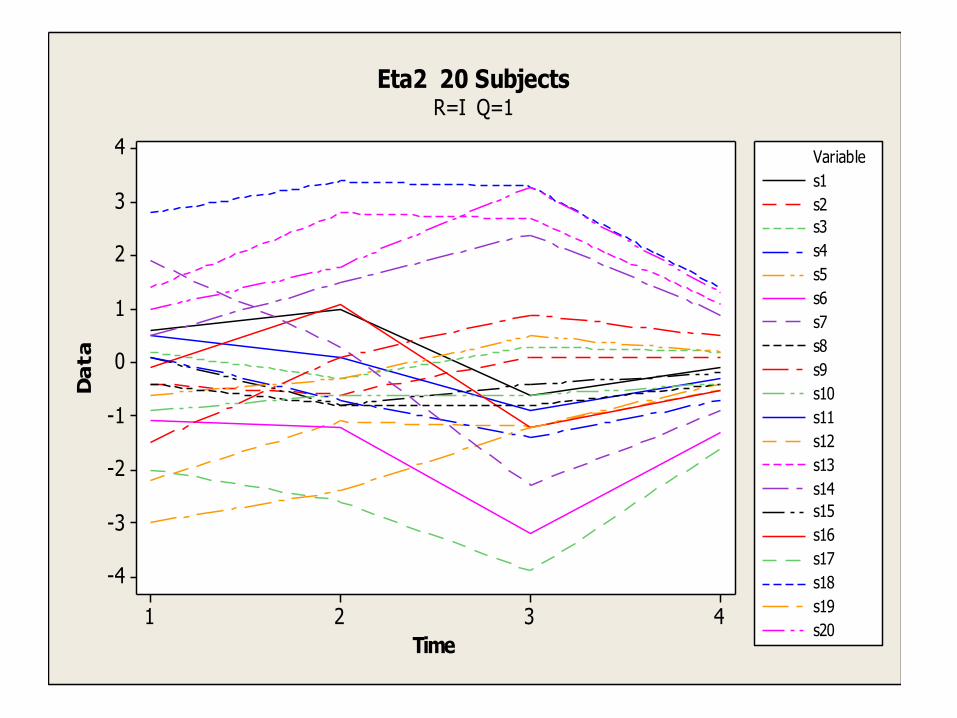
4321

4

3

2

1

0

-1

-2

-3

-4

Time

Da

ta

s10

s11

s12

s13

s14

s15

s16

s17

s18

s19

s1

s20

s2

s3

s4

s5

s6

s7

s8

s9

Variable

Eta2 20 SubjectsR=I Q=1

4321

6

5

4

3

2

1

0

Time

Va

ria

nce

Var1

Var2

Variable

Variance Eta1 & Variance Eta2R(1,1) = .001 R(2,2) = 1.0 Q(1,1) = .001