sorptivity testing to assess durability of concrete...
TRANSCRIPT

Vimal N. Patel
SORPTIVITY TESTING TO ASSESS DURABILITY OF CONCRETE
AGAINST FREEZE-THAW CYCLING
Vimal N. Patel
The Department of Civil Engineering and Applied Mechanics
McGill University
Montreal, Canada
August 2009
A thesis submitted to McGill University in partial fulfilment of the
requirements of the degree of Master of Engineering (Thesis Option)
© Copyright by Vimal N. Patel (2009)

Vimal N. Patel
iii
Vimal N. Patel
ABSTRACT
Current practice assesses the quality of concrete based primarily on
strength. It has been suggested that the quality of concrete should be
characterized not only by strength but also its durability characteristics.
The performance of concrete is greatly affected by its exposure to
aggressive environments, more precisely its transport properties. The
objective of this thesis is to investigate whether sorptivity testing could be
used to assess the durability of concrete against freeze-thaw deterioration.
The research work utilizes various mixture designs, exposure surfaces
and modified testing methods to review the sensitivity of the test and
provide valuable insight into the potential service life behaviour of a mix
design.
iv
Vimal N. Patel
SOMMAIRE
La pratique en vigueur évalue la qualité du béton basée principalement
sur la force. Il a été suggéré que la qualité du béton soit caractérisée non
seulement par la force mais également par ses caractéristiques de
durabilité. La performance du béton est considérablement affectée par son
exposition aux environnements agressifs, plus précisément ses propriétés
de transport. L’objectif de cette thèse est d’étudier si un test d’absorption
pourrait être employé pour évaluer la durabilité du béton contre la
détérioration gel-dégel. Le travail de recherche utilise de diverse
conception de mélange, surfaces d’exposition et méthodes d’essai
modifiées pour réviser la sensibilité du test d’absorption pour fournir une
perspicacité valable dans le comportement potentiel de durée de vie d'une
conception de mélange.

v
Vimal N. Patel
ACKNOWLEDGEMENTS
The author would like to sincerely thank all those involved in the
production of this thesis as well as the experimental work associated with
research.
To begin, I would like to thank my supervisor, Prof. Andrew J. Boyd, McGill
University, for his concise and valuable guidance during the experimental
research work and writing of this thesis. As well as for his financial
assistance that helped keep the focus on work. I would also like to thank
my class colleagues, Mr. Ron Sheppard, laboratory technician, and the
staff members of the materials laboratory of McGill University for their help
in carrying out experimental tasks.
Finally, I would like to thank my family and friends for their tolerance and
support throughout the completion of my studies. I am grateful.

vi
Vimal N. Patel
TABLE OF CONTENT
ABSTRACT........................................................................................................... 3
SOMMAIRE........................................................................................................... 4
ACKNOWLEDGEMENTS .................................................................................. 5
LIST OF FIGURES .............................................................................................. 8
LIST OF TABLES .............................................................................................. 10
INTRODUCTION ................................................................................................ 11
CHAPTER 1 – LITERATURE REVIEW ......................................................... 12 1.1 Theories of Freeze-Thaw ........................................................................................... 12
1.1.1 Hydraulic Pressure (Powers 1945)..................................................................... 12 1.1.2 Osmotic Pressure ........................................................................................................ 15 1.1.3 Litvan’s Theory .............................................................................................................. 16
1.2 Considerations for Freeze-Thaw Resistance............................................... 17 1.2.1 Ice Formation in concrete........................................................................................ 17 1.2.2 Required air-void characteristics ......................................................................... 17 1.2.3 Litvan’s New Theory to frost resistance........................................................... 19 1.2.4 Critical Degree of Saturation .................................................................................. 20
1.3 Influence of Materials (Pigeon & Pleau, 1995)............................................. 21 1.3.1 Portland cement ........................................................................................................... 21 1.3.2 Aggregates ...................................................................................................................... 21 1.3.3 Behaviour of coarse aggregates.......................................................................... 22 1.3.4 Admixtures....................................................................................................................... 25
1.4 Self-Compacting Concrete ....................................................................................... 30 1.4.1 Introduction ..................................................................................................................... 30 1.4.2 Material properties of SCC (Gaimster and Gibbs 2001) ......................... 32 1.4.3 Admixtures and Air-Entrainment .......................................................................... 34
1.5 High Strength Concrete ............................................................................................. 37 1.6 Sorptivity.............................................................................................................................. 43
1.6.1 Water movement in porous materials ............................................................... 43 1.6.2 Water movement in concrete ................................................................................ 45 1.6.3 Absorption Tests .......................................................................................................... 47 1.6.4 Sorptivity Test ................................................................................................................ 49
CHAPTER 2 – EXPERIMENTAL PROGRAM .............................................. 59 2.1 Material Preparation ..................................................................................................... 59
2.1.1 Mixing Equipment and Set Up .............................................................................. 59 2.1.2 Materials ........................................................................................................................... 59 2.1.3 Mixing Procedure ......................................................................................................... 60 2.1.4 Test Specimen Preparation.................................................................................... 61 2.1.5 Specimen testing ......................................................................................................... 61
2.2 Experimental Procedure and Set-up ................................................................. 63 2.2.1 Freeze-Thaw .................................................................................................................. 63 2.2.2 Specimen Pre-conditioning..................................................................................... 65 2.2.3 Sorptivity Testing ......................................................................................................... 66 2.2.4 Density Testing ............................................................................................................. 68
vii
Vimal N. Patel
CHAPTER 3 – RESULTS AND DISCUSSION ............................................. 71 3.1 Influence of materials on performance of mix design ........................... 71 3.2 Sorptivity to assess deterioration due to freeze-thaw cycling ........ 73
3.2.1 Variation of absorption with no air-entraining agent .................................. 73 3.2.2 Variation of absorption in the presence of air-entraining admixtures
79 3.2.3 Early-age and late-age sorptivity indicators................................................... 81
3.3 Freeze-thaw resistance of self-compacting concrete ............................ 82 3.4 Use of AEA in concrete for freeze-thaw resistance................................. 87 3.5 Effect of exposure surface on sorptivity ........................................................ 90 3.6 Effect of sealant on sorptivity ................................................................................ 93
CONCLUSIONS ...............................................................................................100
REFERENCES .................................................................................................102
viii
Vimal N. Patel
LIST OF FIGURES Figure 1: Freezing front ..................................................................................... 13
Figure 2: Relationship between size of capillary pore and freezing temperature of pure water................................................................................. 14
Figure 3: Elongation after 300 cycles versus spacing factor (0.5 w/c) ..... 19
Figure 4: Interaction between air bubbles and cement particles. ............... 27
Figure 5: Image of SCC placed in a small column with congested
reinforcement ...................................................................................................... 30
Figure 6: Typical volume percentage of constituent materials in SCC ...... 33
Figure 7: Mechanism for achieving self-compaction .................................... 35
Figure 8: Relationship between spacing factor and air void content in fresh concrete ............................................................................................................... 37
Figure 9: Schematic of cement paste microstructures at different w/c values ................................................................................................................... 38
Figure 11: Comparison of Portland cement concretes under combined
actions of loading and freeze-thaw cycling .................................................... 40
Figure 12: HSC with 0.25 w/cm, no AE, 2% total air .................................... 41
Figure 13: HSC with 0.25 w/cm, 2.6 g/cwt AE, 5% total air......................... 41
Figure 14: Cumulative absorption i(t) through various wetting regimes ... 44
Figure 15: Absorption curves relative depth of exposure surface .............. 47
Figure 16: Schematic arrangement of ISAT apparatus................................ 48
Figure 17: Schematic arrangement of the CAT method .............................. 49
Figure 18: Schematic arrangement of the Sorptivity test ............................. 50
Figure 19: RH achieved after various periods of pre-conditionings in the environmental chamber at 50oC and 80% RH. The error bars represent
one standard deviation ...................................................................................... 51
Figure 20: RH of the air inside the conditioning containers versus time .. 52
Figure 21: Water leak between the tape and specimen sides .................... 53
Figure 22: Test setup for continuous mass gain monitoring ....................... 54
Figure 23: Sorptivity relative to type of sealant material .............................. 55
Figure 24: Schematic arrangement of in-situ sorptivity testing ................... 56
Figure 27: Freeze-thaw chamber set up......................................................... 65
Figure 28: Pre-conditioning of specimens in environmental chamber....... 65
Figure 29: Variation of permeable pore space over the depth of all mixes............................................................................................................................... 70
Figure 30: Cracking through coarse aggregate in Mix C (SCC - No AEA)73
Figure 32: Effect of F-T cycling on early-age sorptivity of all mixes (0-6
hours) ................................................................................................................... 76
ix
Vimal N. Patel
Figure 33: Effect of F-T cycling on the late-age sorptivity of all mixes (1-8
days) ..................................................................................................................... 76
Figure 34: Effect of freeze-thaw cycling on absorption of Mix C (SCC - No AEA) ..................................................................................................................... 78
Figure 35: Specimen from Mix C (SCC – No AEA) after 100 cycles of freeze-thaw (right) .............................................................................................. 79
Figure 36: Effect of freeze-thaw cycling on absorption of Mix B (Regular - AEA) ..................................................................................................................... 80
Figure 37: Effect of mix design on the average absorption of all mixes at 0
cycles.................................................................................................................... 83
Figure 38: Effect of mix design on the average absorption of all mixes at
50 cycles .............................................................................................................. 83
Figure 39: Freeze-thaw deterioration of SCC beyond 50 cycles ................ 85
Figure 40: Separation of the mortar from the coarse aggregate ................ 86
Figure 41: Effect of mix design on the total absorption at given levels of freeze-thaw cycling ............................................................................................ 88
Figure 42: Specimens from Mix B (Regular - AEA), A (Regular - No AEA), and C (SCC – No AEA) (top to bottom respectively) after 200 freezing and thawing cycles..................................................................................................... 89
Figure 43: Specimen being split by hand after being subjected to 200 freeze-thaw cycles ............................................................................................. 90
Figure 44: Sorptivity curves comparing cast and finished surfaces of Mix C (SCC – No AEA) at 0 cycles of freeze-thaw .................................................. 91
Figure 45: Sorptivity curves comparing cast and finished surfaces of Mix C
(SCC – No AEA) at 50 cycles of freeze-thaw ................................................ 91
Figure 46: Exposure surface of Mix C (SCC - No AEA): a) finished surface
b) cast surface .................................................................................................... 92
Figure 47: Sorptivity curves comparing waxed and taped specimens of Mix B (Regular – AEA) at 150 cycles of freeze-thaw ........................................... 94
Figure 48: Ring absorption phenomenon ....................................................... 95
Figure 49: Poor edge adherence causing capillary suction along edges.. 95
Figure 50: Red dye deposits along curved surfaces of test specimens .... 97
Figure 51: Helical transport path of water ...................................................... 98
Figure 52: Effect of mix design on the total absorption at given levels of
freeze-thaw cycling .......................................................................................... 117
x
Vimal N. Patel
LIST OF TABLES
Table 1: Feature/benefits of SCC Source: (Gaimster 2000) ....................... 32
Table 2: Mixture Designs .................................................................................. 60
Table 3: Fresh concrete slump test and air content test results ................. 61
Table 4: Compressive Strength ....................................................................... 62
Table 5: Freeze-thaw Specimens .................................................................... 64
Table 6: Summary of sorptivity and nick point time for Mix A (Regular - No AEA) ..................................................................................................................... 75
Table 7: Average absorption (mm) of Mix CC (SCC Cast – No AEA) and Mix CF (SCC Finished – No AEA) ................................................................... 92
Table 8: Summary of results of statistical analysis ....................................... 98
1
CHAPTER 1 – LITERATURE REVIEW 11
Vimal N. Patel
INTRODUCTION
From 1994 to 2002, Transports Québec annually invested an average of
$700 million dollars for highway or road conservation and improvement.
The budget is projected to rise to $2 226 million between 2003 and 2013.
The rise in repair costs has been attributed to significant environmental
deterioration caused by freeze-thaw cycling combined with the use of de-
icing chemicals. The importance of environmental condition on concrete
structures should thus not be overlooked during the design phase. Often,
concrete strength has been considered a surrogate for durability.
Unfortunately, it is becoming apparent that this is not particularly true due
to the rising costs for concrete conservation all over the world.
The research objective of this paper is to reinforce the importance of
considering durability properties during the design phase. Mix designs are
considered to have a profound effect on the performance of concrete
structures once in application. The experimental work done in this paper
used a water absorption test to assess the potential durability
characteristics of various concrete mix designs when subjected to freeze-
thaw cycling. The cracking caused by freeze-thaw cycling is assumed to
render a concrete specimen more susceptible to ingress of deleterious
materials; the greater the absorption of these materials, the greater the
potential for corrosion of reinforcing steel and loss of strength due to
cracking.
The experimental work consisted of damaging concrete specimens by
simulating environmental freeze-thaw cycles and assessing the damage
caused by the deterioration mechanism by the means of the ASTM C
1585-04 Standard Test Method for Measurement of Rate of Absorption of
Water by Hydraulic-Cement Concretes (Sorptivity Test). The ASTM
C1585-04 results were then analyzed to validate the applicability of the
Sorptivity Test.
CHAPTER 1 – LITERATURE REVIEW 12
Vimal N. Patel
CHAPTER 1 – LITERATURE REVIEW
1.1 Theories of Freeze-Thaw
1.1.1 Hydraulic Pressure (Powers 1945)
The Hydraulic Pressure Theory, proposed by T.C Powers in 1945,
suggests that the destruction of concrete during freezing is caused by the
hydraulic pressure generated by the expansion of water, rather than direct
pressure due to the growth of ice crystals.
A drop in temperature causes differential freezing of water in the concrete
paste. The formation of ice in capillary pores forces unfrozen water
outwards through the porous medium. Based on Darcy’s model, the flow
of a liquid through a porous medium generates some pressure, and if that
pressure exceeds the tensile resistance of the concrete, cracking will
occur.
This hypothesis is applicable to materials that, at a given temperature,
hold freezable water in two different fashions: first, in small pores that do
not allow the water to freeze, and secondly, in larger pores which do allow
water to freeze. It has been proven experimentally that hardened Portland
cement concrete is considered one of these materials (Powers 2003).
Figure 1 shows that when ice begins to form in region A, the unfrozen
water in that region will move towards the non-saturated region B. As
mentioned previously, the water is not able to move freely into region B.
The flow of water into the porous medium will cause a frictional resistance
and create a hydraulic pressure gradient that follows the laws of hydraulic
flow as proposed by Darcy.
CHAPTER 1 – LITERATURE REVIEW 13
Vimal N. Patel
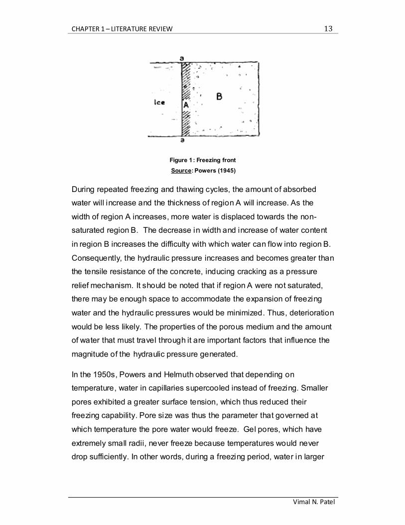
Figure 1: Freezing front
Source: Powers (1945)
During repeated freezing and thawing cycles, the amount of absorbed
water will increase and the thickness of region A will increase. As the
width of region A increases, more water is displaced towards the non-
saturated region B. The decrease in width and increase of water content
in region B increases the difficulty with which water can flow into region B.
Consequently, the hydraulic pressure increases and becomes greater than
the tensile resistance of the concrete, inducing cracking as a pressure
relief mechanism. It should be noted that if region A were not saturated,
there may be enough space to accommodate the expansion of freezing
water and the hydraulic pressures would be minimized. Thus, deterioration
would be less likely. The properties of the porous medium and the amount
of water that must travel through it are important factors that influence the
magnitude of the hydraulic pressure generated.
In the 1950s, Powers and Helmuth observed that depending on
temperature, water in capillaries supercooled instead of freezing. Smaller
pores exhibited a greater surface tension, which thus reduced their
freezing capability. Pore size was thus the parameter that governed at
which temperature the pore water would freeze. Gel pores, which have
extremely small radii, never freeze because temperatures would never
drop sufficiently. In other words, during a freezing period, water in larger

CHAPTER 1 – LITERATURE REVIEW 14
Vimal N. Patel
capillary pores will freeze before water trapped in smaller gel pores since
they are under less stress (Powers 1945).
Figure 2: Relationship between size of capillary pore and freezing temperature of pure water
Source: Pigeon & Pleau 1995
Considering that there exists a discrepancy in pore water freezing
throughout the cement paste, the thermodynamic equilibrium within the
paste is broken when temperatures drop below freezing. Ice has a lower
free energy than liquid water, thus water in the unfrozen gel pores travels
through the porous medium towards levels of lower energy (i.e. ice in the
capillaries). As the water approaches the capillaries and enters regions of
greater pore radius, the freezing temperature increases and water begins
to crystallize.
With this said, the Hydraulic Pressure Theory would depend on:
1) The permeability of the material through which water must flow
to escape the saturated region.
2) The rate of freezing.
3) The amount of water in region A in excess of the critical degree
of saturation.
CHAPTER 1 – LITERATURE REVIEW 15
Vimal N. Patel
1.1.2 Osmotic Pressure
Further research on the volume change of Portland cement during
freezing showed that hydraulic pressure was not the single cause for
deterioration of the cement paste. It was also shown that diffusion of gel
water toward the air voids caused further growth of ice crystals in the
cavities (Powers and Helmuth 1953). Hydraulic pressure and diffusion
would then act simultaneously to cause expansion within the cement
paste.
During a freezing period, the freezable water in a capillary cavity will turn
to ice while, at this point, the water in the gel pores would be supercooled
instead of frozen due to the small size of the pores. As the temperature
drops below the freezing temperature of the water in the capillary pores,
thermodynamic equilibrium is disturbed. The supercooled water in the gel
pores will gain free energy much faster than the ice in the capillary
cavities. Consequently, the gel water has a higher energy potential that
enables it to move toward the ice in the cavity in order to restore
equilibrium. This diffusion of water thus causes expansion of the ice in the
capillary cavity, which in turn can result in expansion of the concrete.
An assumption not previously made in the hydraulic pressure theory is that
the pore water in the capillaries and gel pores is not pure. Pore water in
cement paste contains dissolved chemicals that lower the freezing point of
the solution. As ice forms in a capillary, the concentration of dissolved
chemicals increases in the pore water surrounding the ice crystal. In the
gel pores, the pore water solution is unfrozen and thus has a lower
concentration. The concentration gradient thus forces pore water from the
gel pores to move toward the capillaries. As the pore water from the gel
pores reaches the capillary pore water, the drop in concentration
increases the freezing point thus causing further crystallization of the pore
water in capillaries (Powers 1975).
CHAPTER 1 – LITERATURE REVIEW 16
Vimal N. Patel
1.1.3 Litvan’s Theory
Water absorbed from the surface and contained in the small capillaries
does not freeze due to surface forces that restrict water molecules from
arranging themselves in an order conducive to the formation of a crystal
lattice formation (Litvan 1973).
Litvan first developed a theory which states that there is a forced
movement of water through the cement past due to a difference in vapour
pressure (Litvan 1972). It was further extrapolated to state that when the
temperature drops below 0 oC, water present in large voids will freeze, and
water contained in the smaller capillary voids will be supercooled. The
vapour pressure of water is higher than that of ice. At temperatures below
freezing, supercooled water and ice co-exist and disrupt vapour pressure
equilibrium. Thus, partial emptying of water filled voids equilibrates the
gradient. The emptied water is then forced through the porous medium
towards locations were ice is forming (Litvan 1973). This theory agrees
with Powers in such that high internal stresses caused by liquid movement
in porous medium can cause cracking in the paste. It is noteworthy to
mention that Litvan’s theory suggests that damage can occur in the
absence of any expansion due to ice formation.
The three theories of frost deterioration described may contradict each
other to some extent but are considered to complement more than
contradict each other. The hydraulic pressure theory can be used to
describe the mechanisms that cause tensile forces to act within the
concrete paste due to the movement of water. Litvan’s theory could
correctly describe the reasons for which the water moves within the paste.
Lastly, the osmotic pressure theory could provide a suitable explanation
for the negative effects of deicing agents on deterioration of the concrete
paste (Pigeon 1989).
CHAPTER 1 – LITERATURE REVIEW 17
Vimal N. Patel
1.2 Considerations for Freeze-Thaw Resistance
1.2.1 Ice Formation in concrete
As the temperature decreases, the amount of freezable water in the
cement paste increases at a gradual rate. As mentioned, the amount of
freezable water does not increase instantly as it is dependent on the size
of the pore in which it is contained.
Ice nucleation begins in a pore and the surrounding pore water increases
in concentration as described by the osmotic theory. Pore water contained
in gel pores cannot freeze at temperatures higher than -78 oC (Pigeon
1995). Thus, a system of channels with unfrozen water connects capillary
pores throughout the cement paste. Although capillary pores in a good
quality concrete are discontinuous, the system of channels of unfrozen
water provides water to feed the growth of ice crystals in larger pores
(Adler-Vignes & Dijkema, 1975). This being said, ice formation is directly
related to the amount of freezable water in the concrete. The amount of
freezable water is limited by the initial water to cement ratio. Thus, limitting
the w/c will limit the deterioration of the concrete (Powers 1945).
1.2.2 Required air-void characteristics
Air entrainment is the best-known form of resistance to freeze-thaw
deterioration. Work done by Powers in 1949, and followed up in 1954,
demonstrated that the spacing factor of the air void system was the most
important parameter when determining the effectiveness of air
entrainment. Theoretical spacing factors were determined based on the
hypothesis of the hydraulic pressure theory. The results obtained were in
close agreement with experimental data. It was determined that spacing
factors ranging from 0.254 mm to 0.660 mm provided acceptable frost
resistance to six different pastes cooled at 7 oC per hour. The air
requirements for a given cooling rate depended on paste content, specific
surface of the voids, and spacing factor (Powers 1949).
CHAPTER 1 – LITERATURE REVIEW 18
Vimal N. Patel
Further studies showed that the hydraulic pressures generated during the
freezing of water in large capillary pores increased approximately in
proportion to the square of the distance to the nearest void (Powers and
Helmuth 1953). This statement thus reinforced the requirement of
producing a system of closely spaced air voids. In 1949, Powers’ paper
recommended a spacing factor of 250 m. It was shown that this value
could be adequate for a wide range of concrete and was adopted by many
standards (Pigeon et al. 1986; Pigeon et al. 1985)
Later work by Pigeon (1989) confirmed the 250 m spacing factor
suggested by Powers and also determined that the air void system for a
specific concrete subjected to a certain number of freeze-thaw cycles had
an inherent critical spacing factor. Air void systems with spacing factors
lower than the critical spacing factor demonstrated adequate resistance to
freeze-thaw cycling deterioration. Deterioration of concrete for values
higher than the critical spacing factor increased rapidly. Figure 3 illustrates
the results from the study.

CHAPTER 1 – LITERATURE REVIEW 19
Vimal N. Patel
Figure 3: Elongation after 300 cycles versus spacing factor (0.5 w/c)
Source: (Pigeon and Lachance 1981)
It can be seen from Figure 3, that a concrete specimen with a w/c of 0.5
will show rapid deterioration based on length change for spacing factors
higher than 680 m. The same test showed that for a specimen with a w/c
of 0.6, the critical spacing factor was 570 m (Pigeon and Lachance
1981). Thus, as the w/c ratio of a concrete specimen increases, the critical
spacing factor must decrease to account for the added amount of
freezable water and the porosity of the cement paste. These critical
spacing factors were developed based the on the hydraulic pressure
theory proposed by Powers, in order to account for surface scaling in the
presence of de-icing chemicals. It was found that a spacing factor of 200
m would provide adequate frost resistance for all freeze-thaw
mechanisms (Pigeon 1989).
1.2.3 Litvan’s New Theory to frost resistance
Further research by Litvan showed that even with a spacing factor larger
than 200 m, air entrained concrete in the presence of superplasticizers
CHAPTER 1 – LITERATURE REVIEW 20
Vimal N. Patel
provided good frost resistance. It was suggested that this improved
resistance from air entrainment is due to the increased number of pores in
the volume range of 0.35 – 2.00 m (Litvan 1983).
Superplasticizers tend to reduce the number of large air-entrained
bubbles. Consequently, it was believed that the increased spacing factor
associated with the loss of air voids would reduce frost resistance of
concrete specimens. But as proposed, although the spacing factor of
larger air voids was increased, the spacing between air voids in the 0.35 –
2.00 m remained stable at less than 100 m, significantly smaller than
the suggested distance of 200 m. The effect of superplasticizers on
durability will be further detailed in the following chapter.
1.2.4 Critical Degree of Saturation
A concrete specimen that contains a known amount of freezable water can
withstand a certain amount of freezing and thawing cycles before showing
any signs of deterioration. The water content above which deterioration
begins is called the critical degree of saturation (Powers 1945).
It was initially suggested by Powers that the critical threshold would be
near 90% saturation, suggesting that the remaining 10% of non-saturated
concrete could accommodate the direct pressure caused by the growth of
ice crystals.
Work done by Fagerlund confirmed the existence of a critical degree of
saturation below which concrete subjected to freeze-thaw cycling does not
deteriorate. It was proven that damage occurs after one freezing cycle if
the actual degree of saturation was above the critical threshold, indicating
that frost deterioration is a fracture and not a fatigue phenomenon
(Fagerlund 1971).

CHAPTER 1 – LITERATURE REVIEW 21
Vimal N. Patel
1.3 Influence of Materials (Pigeon & Pleau, 1995)
The materials used in the mix design of concrete influence the frost
resistance of the material. The following text describes the influence of
Portland cement, aggregates, and admixtures on the frost resistance of
concrete.
1.3.1 Portland cement
For a given water to cement ratio and cement content, the chemical and
physical properties of the cement used in the mix greatly affect the
durability of a concrete specimen (Rose et al. 1989).
Cement particles react with water to produce hydration products. These
hydration products provide cohesion and influence the pore size
distribution of the concrete. The type of cement influences the proportions
of hydration products. But just as important, the cement particle size
affects the size distribution of the capillary pores (Rasheeduzzafar 1990).
Finer particles have a larger surface area, which in turn increases the rate
of hydration: there is more cement grain surface accessible to the mixing
water to produce hydration products (Bentz et al. 1999).
As previously described, capillary pore distribution affects the freezing
temperature of water. Cement with a high fineness has a larger number of
particles per unit mass, thus resulting in the preferred formation of smaller
capillary pores. A finer pore size distribution thus lowers the amount of
freezable water since smaller pores drop the freezing temperature to a
level that cannot be achieved under normal climatic conditions. Less
freezable water results in better frost durability. Furthermore, the presence
of fine particles acting as microfillers further reduce pore sizes within the
concrete.
1.3.2 Aggregates
Aggregates are generally classed as fine or coarse aggregates. Concrete
mix designs typically contain a combination of both coarse and fine
CHAPTER 1 – LITERATURE REVIEW 22
Vimal N. Patel
aggregates depending on the use of material. In terms of frost resistance,
fine aggregates are not affected by frost deterioration. This is due to their
small size, which does not allow the development of internal pressures
sufficient to exceed the tensi le resistance of the aggregates. Coarse
aggregates, on the other hand, are more susceptible to freeze-thaw
deterioration. Due to their weight, coarse aggregates are also responsible
for segregation and bleeding in concrete structures. Nonetheless, coarse
aggregates are necessary as they provide shrinkage restraint and a higher
maximum aggregate size provides a higher strength concrete due to lower
cement demands.
1.3.3 Behaviour of coarse aggregates
Coarse aggregates can deteriorate concrete in two different ways: sound
aggregates can expel water during freeze-thaw cycling which
subsequently deteriorates the cement paste, secondly unsound
aggregates can themselves deteriorate from freeze-thaw cycling and
decrease the strength of the concrete.
There exist three parameters that determine the frost resistance of
aggregates; the elastic accommodation, the critical size and the critical
degree of saturation. (Verbeck and Landgren, 1960). The following text will
further discuss these parameters in detail.
Although often assumed, aggregates are not completely rigid. Sound
aggregates are considered to have a low permeability. Thus , during
freeze-thaw cycling the pore water inside the aggregate cannot be readily
expelled. The expansive pressure caused by the freezing of pore water
must then be relieved by an increase in volume of the aggregate particle.
The expansion of the aggregate to account for the increase in volume from
the formation of ice is called elastic accommodation. The following
expression describes the internal pressure caused by the freezing of water
(Verbeck and Landgren, 1960).
CHAPTER 1 – LITERATURE REVIEW 23
Vimal N. Patel
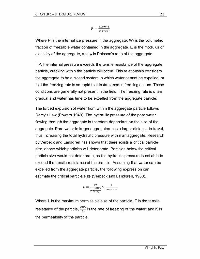
Where P is the internal ice pressure in the aggregate, Wf is the volumetric
fraction of freezable water contained in the aggregate, E is the modulus of
elasticity of the aggregate, and is Poisson’s ratio of the aggregate.
If P, the internal pressure exceeds the tensile resistance of the aggregate
particle, cracking within the particle will occur. This relationship considers
the aggregate to be a closed system in which water cannot be expelled, or
that the freezing rate is so rapid that instantaneous freezing occurs. These
conditions are generally not present in the field. The freezing rate is often
gradual and water has time to be expelled from the aggregate particle.
The forced expulsion of water from within the aggregate particle follows
Darcy’s Law (Powers 1949). The hydraulic pressure of the pore water
flowing through the aggregate is therefore dependant on the size of the
aggregate. Pore water in larger aggregates has a larger distance to travel,
thus increasing the total hydraulic pressure within an aggregate. Research
by Verbeck and Landgren has shown that there exists a critical particle
size, above which particles will deteriorate. Particles below the critical
particle size would not deteriorate, as the hydraulic pressure is not able to
exceed the tensile resistance of the particle. Assuming that water can be
expelled from the aggregate particle, the following expression can
estimate the critical particle size (Verbeck and Landgren, 1960).
Where L is the maximum permissible size of the particle, T is the tensile
resistance of the particle, is the rate of freezing of the water; and K is
the permeability of the particle.
CHAPTER 1 – LITERATURE REVIEW 24
Vimal N. Patel
Both previous parameters assume that the aggregate particles are fully
saturated. Thus, the onset of deterioration would begin immediately upon
freeze-thaw cycling. Generally, concrete in field conditions is not fully
saturated. The frost resistance of the aggregate is dependant on the
degree of saturation because, as with cement paste, there exists a critical
degree of saturation below which the aggregate would contain sufficient
empty space to accommodate the expansion of freezing water. Thus, like
cement paste, the aggregate resistance to frost deterioration is highly
dependent on its permeability, pore structure, air content, relative
humidity, etc.
As the degree of saturation of the aggregate particle is an important
parameter for frost resistance, the porosity of the particle will influence its
frost resistance. Aggregates can be grouped into three levels of porosity;
high porosity, low porosity, and intermediate porosity.(Pigeon & Pleau,
1995)
Aggregates with very low porosity generally exhibit high frost resistance.
They are often not saturated and if they are fully saturated the amount of
freezable water is negligible since it would not develop significant
pressures to disrupt the aggregate.
Aggregates with a very high porosity also generally have good frost
resistance, as they provide sufficient drainage properties to prevent
hydraulic pressures from developing. These aggregates are rarely critically
saturated under field conditions (Pigeon & Pleau, 1995).
Intermediate porosity aggregates are generally frost susceptible particles.
These particles have pores large enough to reach critical saturation but
too small to relieve the hydraulic pressures caused by the freezing of
water. (Pigeon & Pleau, 1995)
CHAPTER 1 – LITERATURE REVIEW 25
Vimal N. Patel
1.3.4 Admixtures
1.3.4.1 Air-Entraining Agents
Air entraining agents (AEA) are used to stabilize the air void system of a
concrete mix. These admixtures are used during the mixing process while
the concrete is in a plastic state. Air entrainment is considered to be the
most important characteristic when discussing the frost resistance of
concrete. It has been suggested that the air content be 25% of the cement
paste (cement + water) to provide adequate frost resistance (Chatterji
2003).
Air-entraining admixtures reduce the energy required to break down air
voids into smaller voids. They do so by reducing the surface tension of
water, which reduces the energy required to form new bubbles. Air
entraining admixtures are surface-active agents, long molecules that have
a hydrophilic and a hydrophobic end. The hydrophilic end tends to attract
water and the hydrophobic end repels water. Thus, air-entraining agents
lower surface tension, concentrate at air water interfaces, and stabilize
already existing air voids (Mindess 1981) Surface energy is the key
parameter when discussing the air void system of concrete. Surface
energy is the product of the surface tension and the surface area of any
material. The formation of bubbles during the mixing of fresh concrete
produces air voids that possess an associated amount of energy (Pigeon
1995). The bubbles formed during the mixing process require energy to
divide into two voids with an equivalent volume. When energy is put into
the system, the larger air void can divide into two smaller air voids with an
equivalent volume. The advantage of the latter is that the two smaller air
voids have a larger surface area as well as a decreased spacing factor
within the concrete mix.
The mixing process creates shearing forces that subdivide larger voids
and create smaller voids. For a given volume, smaller voids have a lower
spacing factor than larger voids (Pigeon 1995) and as previously
CHAPTER 1 – LITERATURE REVIEW 26
Vimal N. Patel
discussed, the frost resistance of concrete increases with the decrease in
air void spacing. AEA’s facilitate the formation of air voids during the
mixing process thus increasing the number of smaller air voids and
increasing frost resistance. Furthermore, larger voids are prone to
escaping the concrete due to hydrostatic pressures that push the bubble
upward and out of the mix. The deterring agent responsible for keeping
these voids in the mix is surface friction. Surface friction increases with an
increase in surface area. As mentioned previously, for a given volume, two
smaller voids will have a larger surface area than one larger void, and so
smaller voids will tend to remain in the mix as they will have more surface
friction to resist hydrostatic pressures pushing the bubbles upwards.
The production of several smaller voids is not sufficient on its own. As any
system will tend towards a lower state of free energy, smaller voids will
tend to coalesce and re-produce larger air voids. Thus, air-entraining
agents must also stabilize the already formed air voids. In Figure 4, the
hydrophilic end of air entraining molecules are absorbed at the air-water
interface; this decreases the surface tension and produces an elastic film
around the bubble (Mielenz et al. 1958a). This elastic film helps resist
coalescence during collisions during the mixing process. Cement particles
are positively charged. The hydrophobic end of the air-entraining agent is
negatively charged and it has been suggested that this end causes the air
voids to be bound to the paste (i.e. cement particles are attracted to the air
voids) (Mielenz et al. 1958a).

CHAPTER 1 – LITERATURE REVIEW 27
Vimal N. Patel
Figure 4: Interaction between air bubbles and cement particles.
Source: (Du and Folliard 2005)
In short, effective air entraining admixtures must reduce surface tension
and produce a highly elastic film around air bubbles. This film must reduce
air transfer from smaller air voids to larger ones so that air void surface
area is not compromised. To remain stable, the surface active agents of
air entraining admixtures must be bound to particles of the cement paste
and not deteriorate over time (Mielenz et al. 1958b).
An external parameter that strongly influences the stability of the air void
system is viscosity of the cement paste (Pigeon 1989). Movement of air
voids decreases as the viscosity of a mix increases. With less movement,
there is less coalescence and air voids are better retained in the mix.
Cement can also influence air entrainment in a physical manner. The
stability of air voids within the cement paste depends on their adherence
to solid particles (Bruere 1955). It has been found that the fineness of the
cement grain is the physical effect that influences air entrainment. Finer
cements have a larger surface area to be covered by water. This higher
water demand by fine cement decreases the amount of water available to
form air voids and thus entraining air becomes more difficult. Likewise it
should be noted that a paste with high cement fineness will also have a
higher viscosity. As mentioned, the high viscosity paste would provide
CHAPTER 1 – LITERATURE REVIEW 28
Vimal N. Patel
cushion effects that enable air bubbles to absorb shocks and prevent
coalescence. Thus, air void stability is enhanced with finer cement
particles (Du and Folliard 2005).
Furthermore, mineral admixtures can also physically affect air entrainment
in a concrete mix. As with cement, fine admixture particles have the same
influence on viscosity as fine cement particles.
Aggregates also influence the viscosity of the mix. A large quantity of fine
aggregate increases the viscosity of the mix and thus creates a ―grid
effect‖ that physically prevents the escape of air voids (Powers, 1964).
Other chemical admixtures can also affect air entrainment. Today,
concrete mix designs often contain superplasticizers, retarding agents and
accelerators. Water reducers and superplasticizers reduce the amount of
cement required. They increase the fluidity of the paste but consequently
increase the risk of coalescence and loss of air voids. Also,
superplasticizers increase repulsive forces between cement particles and
thus weaken the binding of air voids to cement grains. This reduced
binding thus increases the tendency for air voids to coalesce.
The water to cement ratio has a physical effect on the formation of air
voids in concrete. The size of the air voids decreases with w/c (Backstrom
et al. 1958). A concrete mix with a lower w/c will have a higher viscosity;
wherein the higher viscosity translates into a reduction in air void
coalescence. However, the stiffer the mix, the more difficult it becomes to
entrain air. This is because there is a higher energy demand to shear air
bubbles in the concrete mix. But it should also be noted that the air
content required to obtain satisfactory durability performance decreases
with water to cement ratio (Mielenz et al. 1958c).
Mixing, placing and finishing techniques also play an important role in air
entrainment efficiency. Air entrainment occurs during the mixing process.
CHAPTER 1 – LITERATURE REVIEW 29
Vimal N. Patel
The mixing stage should thus be long enough to ensure adequate air
entrainment of a concrete mix (Powers 1964).
Compaction or consolidation does not significantly affect the spacing
factor of entrained air. When a concrete mix is vibrated, it is primarily the
larger air voids that are expelled. Thus, properly air entrained concrete is
little affected by vibration (Backstrom 1958)
1.3.4.2 Water-Reducing Admixtures
Some water-reducing admixtures can act like air-entraining admixtures
since they entrain air voids during the mixing process. The presence of air
voids thus increases workability without an increase in water content to
compromise concrete strength. The difference in the air voids produced
with water–reducing admixtures versus air-entrained admixtures is the
size and spacing of the air voids. Water-reducing admixtures create air
voids that are much larger than air-entrained air voids. Also, the spacing
factor ranges from 400 to 800 m. (Pigeon & Pleau, 1995). Thus concrete
with water-reducing admixtures do not have effective protection against
freeze-thaw deterioration.
1.3.4.3 Superplasticizers
Superplasticizers are essentially high-range water reducing admixtures.
These admixtures enable the production of flowing concrete and enable
the formulation of high strength concrete for a given workability.
Superplasticizers can provide sufficient workability even at very low water
to cement ratios. Considering what has been previously discussed, there
exists conflicting results regarding the effect of superplasticizers on the air
void system of a concrete mix. It has been shown that superplasticizers do
not have an effect on the critical spacing factor of concrete (Pigeon 1989).
Two identical concrete specimens, one with and one without
superplasticizers were tested and showed no significant difference in
critical spacing factor. Further work done by Pigeon and Langlois (1991)

CHAPTER 1 – LITERATURE REVIEW 30
Vimal N. Patel
demonstrated that superplasticizers do not have an effect on the
resistance to freeze-thaw deterioration. Two similar concrete mixes, one
with and one without superplasticizers were subjected to 300 rapid freeze-
thaw cycles and no significant differences existed between the two.
The following chapter further discusses the role of superplasticizers in the
development of concrete durability.
1.4 Self-Compacting Concrete
1.4.1 Introduction
The compaction of concrete plays a major role in the development of a
dense matrix capable of providing concrete its strength. Adequate
compaction is achieved through vibration in the field, which removes large
air voids to produce a hardened concrete with the adequately prescribed
air content. Concrete is often placed in regions where compaction is
impractical. As seen in Figure 5, virtually every concrete structure contains
steel reinforcement and congested steel reinforcement configurations
make it difficult to place and properly compact concrete. These issues
have moved research towards the development of self-compacting
concrete (SCC).
Figure 5: Image of SCC placed in a small column with congested reinforcement
Source: (Gaimster 2000)
CHAPTER 1 – LITERATURE REVIEW 31
Vimal N. Patel
Initial attempts to design a self-compacting concrete had cement contents
that often reached 450 kg/m3. The side effects of such high cement
contents, such as segregation and bleeding, along with the expensive
cement rich mixes restricted the use of early SCC’s (Bartos and Grauers
1999). The development of more applicable superplasticizers, admixtures
and viscosity modifiers has greatly increased the range of application of
SCC. Superplasticizers produce sufficient workability and various
viscosity-modifying agents provide enough cohesion to prevent washout.
A concrete mix must possess the following three characteristics to be
deemed an SCC:
1) Filling ability: The concrete mix must be able to flow under i ts own
weight into the formwork. This property can be measured through
slump-flow tests.
2) Passing ability: In addition to flowing under its own weight, the
concrete mix must be able to pass through tight openings (e.g.
between reinforcing bars)
3) Resistance to segregation: with properties 1) and 2) being met,
segregation becomes an important issue. It is critical that the mix
provide adequate segregation resistance.
Resistance to segregation typically becomes the major difficulty in such
that a compromise must be made between high fluidity and cohesion of
the fresh SCC mix. Work done in Japan in the late 1980’s by Okamura
achieved SCC mixes that incorporated the three key characteristics as
mentioned above. Since then, SCC has gained increased popularity
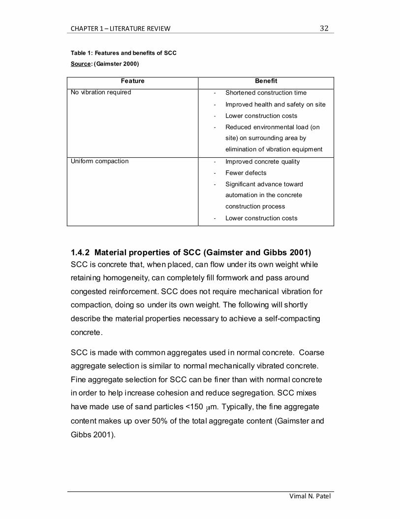
worldwide (Gaimster 2000; Henderson 2000). Table 1 summarizes the
features and benefits of SCC.
CHAPTER 1 – LITERATURE REVIEW 32
Vimal N. Patel
Table 1: Features and benefits of SCC
Source: (Gaimster 2000)
Feature Benefit
No vibration required - Shortened construction time
- Improved health and safety on site
- Lower construction costs
- Reduced environmental load (on
site) on surrounding area by
elimination of vibration equipment
Uniform compaction - Improved concrete quality
- Fewer defects
- Significant advance toward
automation in the concrete
construction process
- Lower construction costs
1.4.2 Material properties of SCC (Gaimster and Gibbs 2001)
SCC is concrete that, when placed, can flow under its own weight while
retaining homogeneity, can completely fill formwork and pass around
congested reinforcement. SCC does not require mechanical vibration for
compaction, doing so under its own weight. The following will shortly
describe the material properties necessary to achieve a self-compacting
concrete.
SCC is made with common aggregates used in normal concrete. Coarse
aggregate selection is similar to normal mechanically vibrated concrete.
Fine aggregate selection for SCC can be finer than with normal concrete
in order to help increase cohesion and reduce segregation. SCC mixes
have made use of sand particles <150 m. Typically, the fine aggregate
content makes up over 50% of the total aggregate content (Gaimster and
Gibbs 2001).
CHAPTER 1 – LITERATURE REVIEW 33
Vimal N. Patel
Proportions of cement and fine fillers are higher than in typical concrete as
they increase cohesion and stability of the mix; along with cement
admixtures which are essential to providing adequate flow and workability
of the mix. Superplasticizers play a key role in increasing the workability of
the mix but often compromise cohesion at high dosages. A viscosity-
modifying admixture often accompanies the addition of superplasticizers to
retain cohesion and prevent washout.
As with normal concrete, water plays a significant role in the density of the
hydrated cement paste and the overall strength and durability of the
hardened concrete. Often, improper site mixing is the consequence of
adding water to achieve workability. With SCC, any added water will
encourage washing out and increases the risk of segregation. Considering
that segregation and bleeding resistance are the most difficult parameters
to achieve in SCC, it is imperative to control water addition in SCC mixes.
Thus, it is recommended that free water content remain under 200 litres
per cubic metre of concrete and that the water to cementitious materials
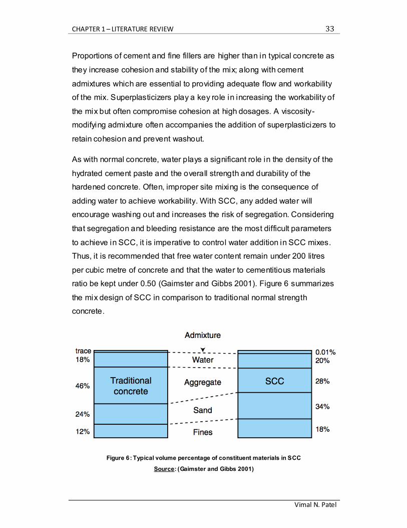
ratio be kept under 0.50 (Gaimster and Gibbs 2001). Figure 6 summarizes
the mix design of SCC in comparison to traditional normal strength
concrete.
Figure 6: Typical volume percentage of constituent materials in SCC
Source: (Gaimster and Gibbs 2001)
CHAPTER 1 – LITERATURE REVIEW 34
Vimal N. Patel
When compared to traditional concrete with the same water to cement
ratio, the compressive strength of SCC is similar. SCC mixes are designed
with high fines content and lower water to cement ratio and can reach
strengths up to 60 MPa (Gaimster and Gibbs 2001). Thus, high
compressive strength is often not difficult to achieve in SCC.
1.4.3 Admixtures and Air-Entrainment
1.4.3.1 Viscosity Modifying Admixtures
As mentioned, viscosity modifying admixtures (VMA) are added to an SCC
mix to increase cohesion and resistance to segregation and bleeding.
Welan gum, a kind of natural polysaccharide has proven to be effective
and is a commonly used VMA (Rols et al. 1999). Given its high cost,
however, the industry has been looking for alternatives that could provide
similar results. New lower cost VMA’s such as starch, precipitated silica,
and other by-products from the starch industry were emerging in the late
1990’s, which increased the importance of understanding the effect of
these VMA’s on the performance of hardened SCC.
Mixtures that contain VMA’s behave in a pseudo plastic manner, in which
the viscosity decreases with an increase in shear rate. The force exerted
on the mixture decreases its viscosity and causes it to flow more like
water. For mixtures containing a VMA, viscosity is built-up through the
association and entanglement of polymer chains in the VMA at a low
shear rate. This property increases the stability of concrete and reduces
the risk of segregation after casting (Lachemi et al. 2004b). Such viscosity
is necessary to avoid the blockage of coarse aggregates when the
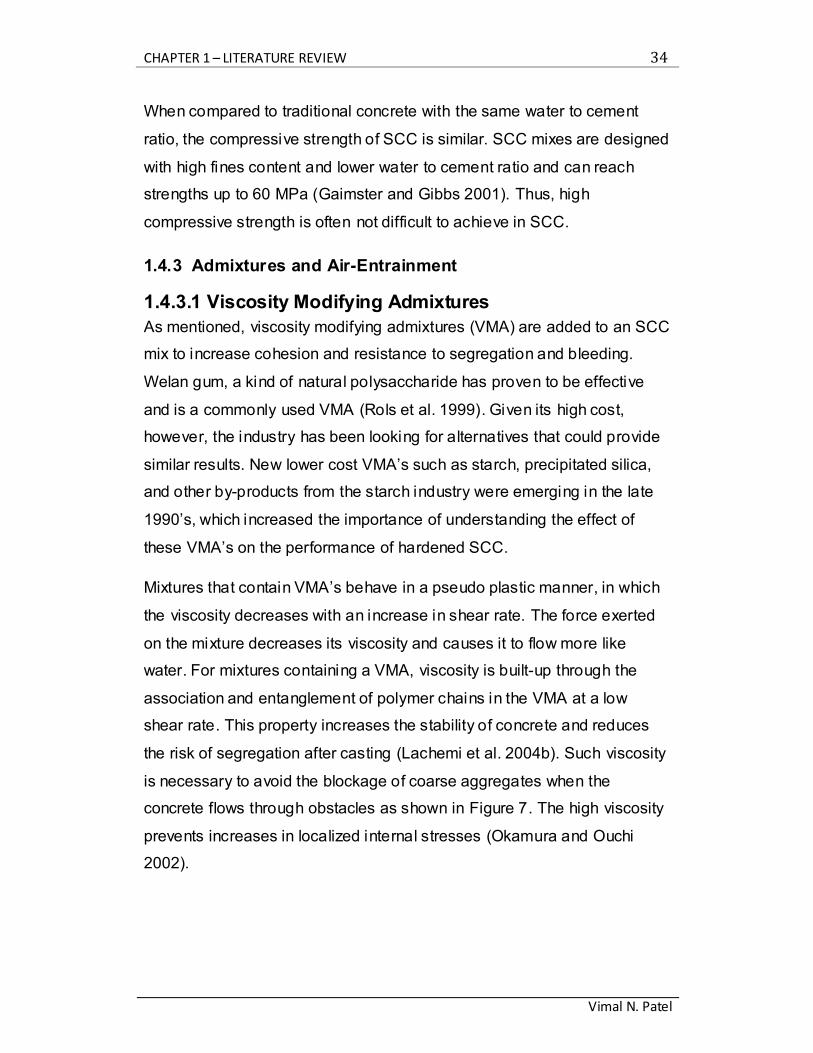
concrete flows through obstacles as shown in Figure 7. The high viscosity
prevents increases in localized internal stresses (Okamura and Ouchi
2002).
CHAPTER 1 – LITERATURE REVIEW 35
Vimal N. Patel
Figure 7: Mechanism for achieving self-compaction
Source: (Okamura and Ouchi 2002)
Research has been done to determine the compatibility of various VMA ’s
with a range of superplasticizers (SP) (Lachemi et al. 2004a). It has been
shown that washout resistance increases with an increase in VMA content
and decrease in SP content. Along these lines, most research involving
VMA and SCC focuses on the effect of the admixtures on the fluidity,
segregation and washout resistance of the cement paste.
Less commonly discussed are the durability properties of SCC containing
VMA. Since VMA’s have little activity at the air/water interface due to their
lack of hydrophobic constituents, they do not generate foam or entrap
large volumes of air voids (Khayat 1995). Consequently, the presence of
VMA requires a greater addition of air-entraining agent (AEA) to secure a
given air volume. As well, the air-entrainment of SCC can significantly
reduce the viscosity of the paste; this then reduces its cohesiveness and
resistance to segregation. An SCC susceptible to washout can affect the
stability of the air-void system and impair the ability to maintain small and
closely spaced air voids in fresh concrete (Khayat 2000). Lack of an
CHAPTER 1 – LITERATURE REVIEW 36
Vimal N. Patel
adequate air-void system would result in a significant reduction in frost
durability.
Further work done by Yamato et al. has shown that mixes with 0.45 w/c
ratio containing VMA exhibited poor frost durability. This was explained by
the fact that mixes containing VMA had a greater porosity compared to
control mixes without VMA. Porosity measured using mercury intrusion
porosimetry for mixes with VMA ranged from 58.9 to 71.7 mm3/g
compared to 56.1 mm3/g found in a control mix with no VMA. Along with a
higher porosity, the mixes containing VMA had a larger concentration of
capillary pores that were larger than 10 nm (Khayat 1995; Yamato et al.
1991).
Khayat and Assaad have shown that air void stability can be obtained in
optimized SCC mix designs and proper agitation. They warned that the
addition of VMA and high range water reducing admixtures in SCC mixes
should be done with caution in order to ensure proper air-void stability in
self-consolidating concrete (Khayat and Assaad 2002).
The typical mix design approach for normal concrete is to produce a cost
effective mix that will provide adequate performance criteria such as
strength or durability once hardened. The mix design for SCC differs in
that the key parameter in mix design becomes flowability. An SCC mix
must flow under its own weight without blocking and still provide the
necessary performance criteria once hardened.
1.4.3.2 Superplasticizers
Although further research is needed to determine the effect of
superplasticizers on the air-void stability of concrete, it has been
mentioned that superplasticizers (SP) are an important cause of instability
in the spacing factor. Larger air void formation due to coalescence of air
voids results in a coarser air void system. The effect of SP on air void
stability is highly variable and is influenced by many parameters such as
CHAPTER 1 – LITERATURE REVIEW 37
Vimal N. Patel
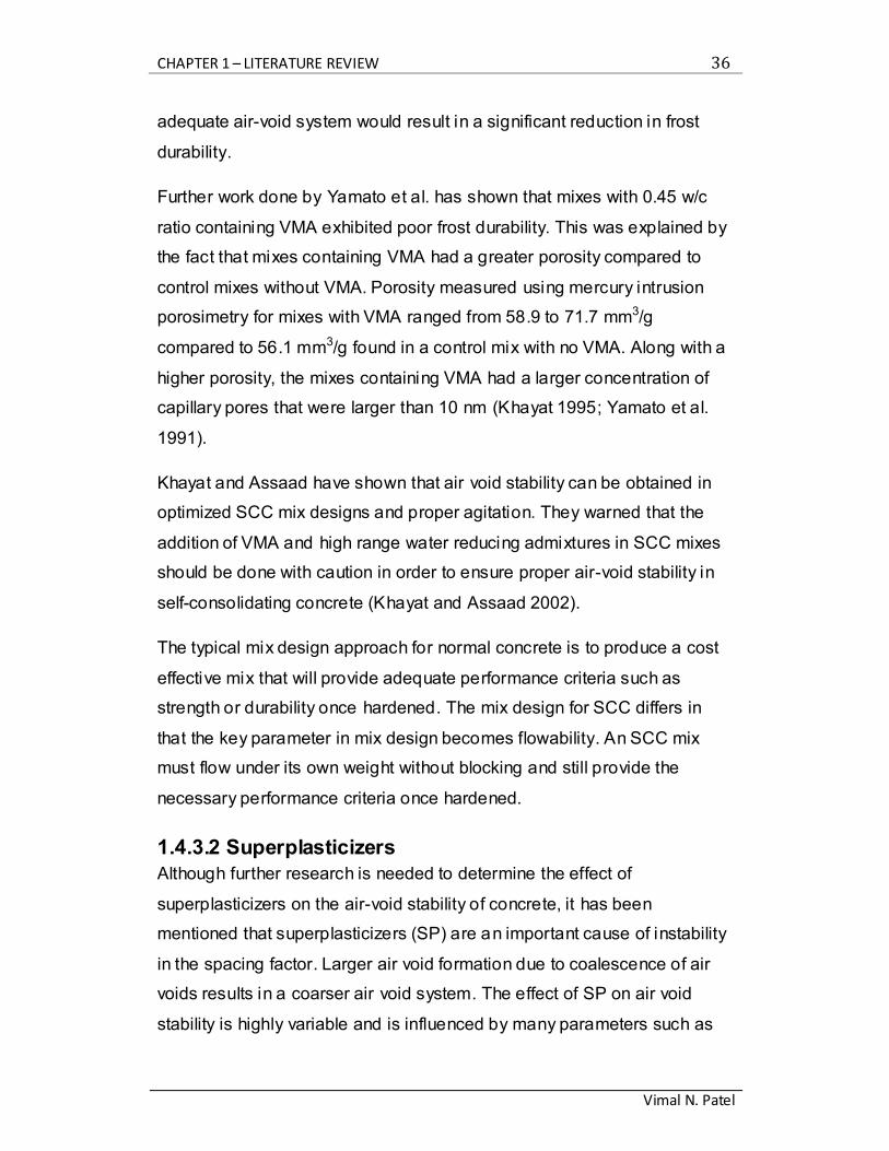
the type of air entrainment and the characteristics of the cement (Plante et
al. 1989). Field tests have shown even greater discrepancies between air
void content and spacing factor relationships.
Figure 8: Relationship between spacing factor and air void content in fresh concrete
Source: (Saucier et al. 1990)
Thus, concrete producers should be very careful when designing air-
entrained mixes containing SP as the air-void system can be destabilized
even though the total air content does not change significantly (Saucier et
al. 1990).
1.5 High Strength Concrete
In the 1970s, a spike in concrete bridge deck cracking motivated the use
of higher strength concrete. High strength concrete (HSC) has a lower w/c
than normal strength concrete. Consequently, there are more cement
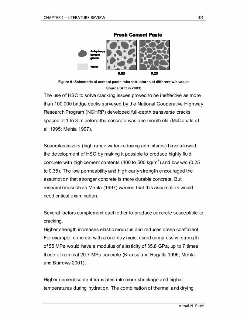
grains and less water per unit volume (Aïtcin 2003). This creates a very
compact and dense microstructure with reduced porosity and low
permeability. Figure 9 illustrates the difference between the
microstructure of conventional strength concrete (0.65 w/c) and high
strength concrete (0.25 w/c).
CHAPTER 1 – LITERATURE REVIEW 38
Vimal N. Patel
Figure 9: Schematic of cement paste microstructures at different w/c values
Source:(Aïtcin 2003)
The use of HSC to solve cracking issues proved to be ineffective as more
than 100 000 bridge decks surveyed by the National Cooperative Highway
Research Program (NCHRP) developed full-depth transverse cracks
spaced at 1 to 3 m before the concrete was one month old (McDonald et
al. 1995; Mehta 1997).
Superplasticizers (high range water-reducing admixtures) have allowed
the development of HSC by making it possible to produce highly fluid
concrete with high cement contents (400 to 500 kg/m3) and low w/c (0.25
to 0.35). The low permeability and high early strength encouraged the
assumption that stronger concrete is more durable concrete. But
researchers such as Mehta (1997) warned that this assumption would
need critical examination.
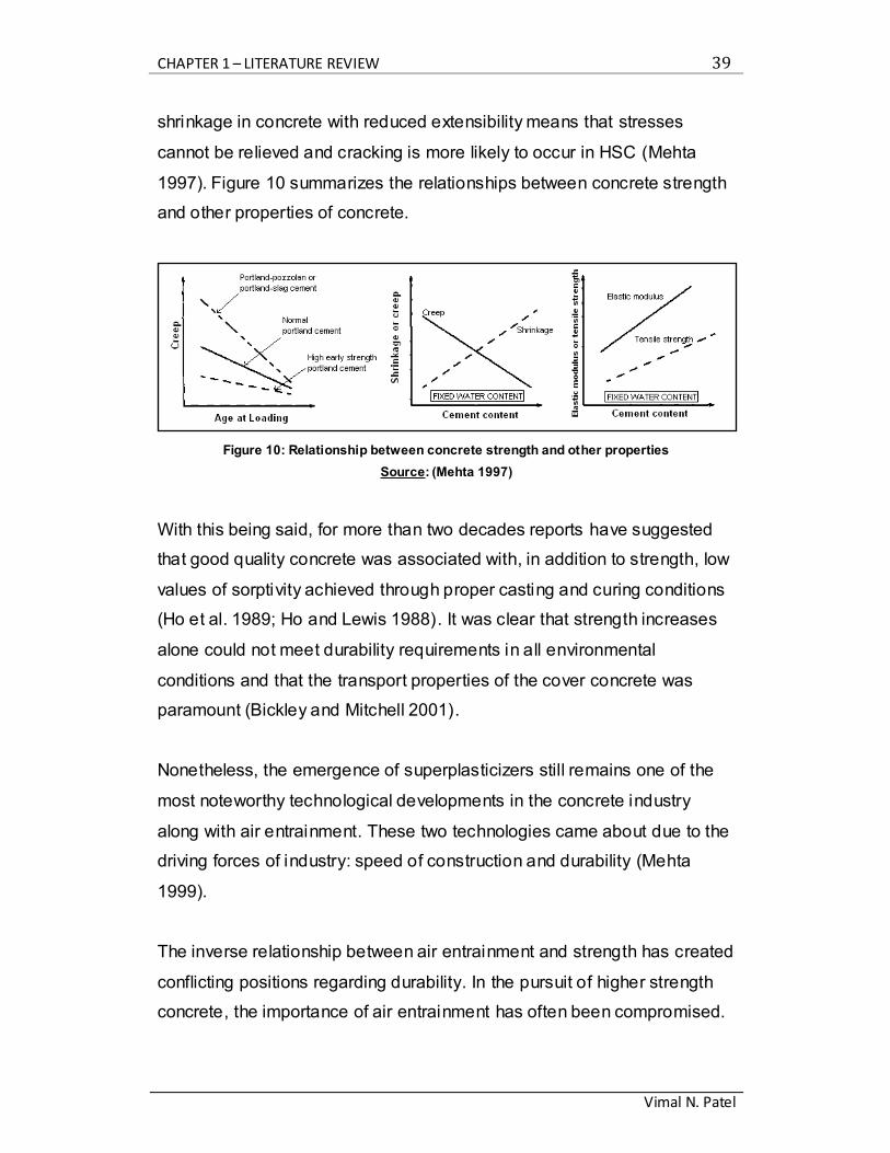
Several factors complement each other to produce concrete susceptible to
cracking.
Higher strength increases elastic modulus and reduces creep coefficient.
For example, concrete with a one-day moist cured compressive strength
of 55 MPa would have a modulus of elasticity of 35.8 GPa, up to 7 times
those of nominal 20.7 MPa concrete (Krauss and Rogalla 1996; Mehta
and Burrows 2001).
Higher cement content translates into more shrinkage and higher
temperatures during hydration. The combination of thermal and drying
CHAPTER 1 – LITERATURE REVIEW 39
Vimal N. Patel
shrinkage in concrete with reduced extensibility means that stresses
cannot be relieved and cracking is more likely to occur in HSC (Mehta
1997). Figure 10 summarizes the relationships between concrete strength
and other properties of concrete.
Figure 10: Relationship between concrete strength and other properties
Source: (Mehta 1997)
With this being said, for more than two decades reports have suggested
that good quality concrete was associated with, in addition to strength, low
values of sorptivity achieved through proper casting and curing conditions
(Ho et al. 1989; Ho and Lewis 1988). It was clear that strength increases
alone could not meet durability requirements in all environmental
conditions and that the transport properties of the cover concrete was
paramount (Bickley and Mitchell 2001).
Nonetheless, the emergence of superplasticizers still remains one of the
most noteworthy technological developments in the concrete industry
along with air entrainment. These two technologies came about due to the
driving forces of industry: speed of construction and durability (Mehta
1999).
The inverse relationship between air entrainment and strength has created
conflicting positions regarding durability. In the pursuit of higher strength
concrete, the importance of air entrainment has often been compromised.
CHAPTER 1 – LITERATURE REVIEW 40
Vimal N. Patel
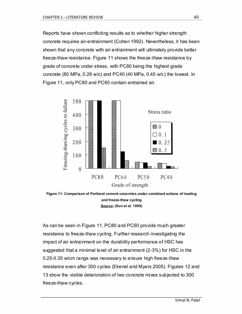
Reports have shown conflicting results as to whether higher strength
concrete requires air-entrainment (Cohen 1992). Nevertheless, it has been
shown that any concrete with air entrainment will ultimately provide better
freeze-thaw resistance. Figure 11 shows the freeze-thaw resistance by
grade of concrete under stress, with PC80 being the highest grade
concrete (80 MPa, 0.26 w/c) and PC40 (40 MPa, 0.45 w/c) the lowest. In
Figure 11, only PC80 and PC60 contain entrained air.
Figure 11: Comparison of Portland cement concretes under combined actions of loading
and freeze-thaw cycling
Source: (Sun et al. 1999)
As can be seen in Figure 11, PC80 and PC60 provide much greater
resistance to freeze-thaw cycling. Further research investigating the
impact of air entrainment on the durability performance of HSC has
suggested that a minimal level of air entrainment (2-3%) for HSC in the
0.25-0.35 w/cm range was necessary to ensure high freeze-thaw
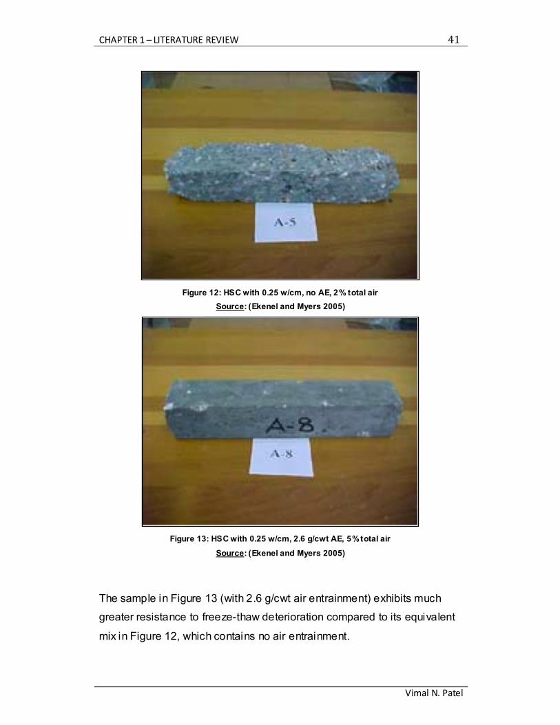
resistance even after 300 cycles (Ekenel and Myers 2005). Figures 12 and
13 show the visible deterioration of two concrete mixes subjected to 300
freeze-thaw cycles.
CHAPTER 1 – LITERATURE REVIEW 41
Vimal N. Patel
Figure 12: HSC with 0.25 w/cm, no AE, 2% total air
Source: (Ekenel and Myers 2005)
Figure 13: HSC with 0.25 w/cm, 2.6 g/cwt AE, 5% total air
Source: (Ekenel and Myers 2005)
The sample in Figure 13 (with 2.6 g/cwt air entrainment) exhibits much
greater resistance to freeze-thaw deterioration compared to its equivalent
mix in Figure 12, which contains no air entrainment.
CHAPTER 1 – LITERATURE REVIEW 42
Vimal N. Patel
Micro-cracks in concrete have a higher probability of forming at the
interfacial transition zone and, once formed, can bridge from one
aggregate to another. This network of micro-cracks becomes a very
effective transport mechanism. It has been noted that micro-crack
concentration is higher in high strength concrete than in normal concrete
(Damgaard Jensen and Chatterji 1996). The increased concentration of
micro-cracks suggests that HSC is more susceptible to damage during
freeze-thaw cycling.
Tests investigating water uptake and ice formation in concrete before and
after freeze-thaw cycling have showed that even small increases in
freezable water in concrete can lead to very large levels of deterioration.
However, the increase of freezable water in high strength concrete after
freeze-thaw cycling was lower than that of normal strength concrete
(Jacobsen et al. 1996).
What can be agreed upon is the effect of crack formation on transport
properties. Crack width displacements larger than 50 microns greatly
increase the permeability of concrete (Aldea et al. 1999; Wang et al.
1997). Durable concrete is achieved through the reduction of crack
formation. This has been reinforced in Canadian codes, where concrete
strength has been limited to 85 MPa, and it has been pointed out that
higher strength concretes vary in their bri ttleness and need for increased
confinement to improve their ductility (Bickley and Mitchell 2001). These
provisions were supported by data showing a tendency of splitting cracks
in high strength concrete columns that resulted in premature spalling
(Collins 1993).
General recommendations to reduce cracking in concrete include lowered
cement contents, good quality low shrinkage aggregates, air entrainment,
and low water to cement ratios. Due high heat production during hydration,
CHAPTER 1 – LITERATURE REVIEW 43
Vimal N. Patel
many transportation agencies recommend limiting cement content to 335
kg/m3 in order to lower the probability of cracking (McDonald et al. 1995).
An increase in concrete strength alone is not considered to be sufficient.
Greater concrete quality can only come from a collective increase in
strength and durability to respond to the new requirements of building
structures around the world (Neville and Aïtcin 1998).
1.6 Sorptivity
1.6.1 Water movement in porous materials
Many building materials used in the construction industry are porous. The
ingress of moisture and the transport properties of these materials have
become the underlying source for many engineering problems such as
corrosion of reinforcing steel, and damage due to freeze-thaw cycling or
wetting and drying cycles. In the 1970’s, Hall suggested the importance of
studying the unsaturated flow of water in porous mediums. The capillary
potential (suction), the water diffusivity (D), and the hydraulic
conductivity (K) were stated as being the three key parameters that
needed further investigation (Hall 1977). Following this, research was
conducted to devise experimental methods to quantify and model
transport properties. Sorptivity was introduced as a testing method that
consisted of a uni-directional water absorption front within a specimen.
The cumulative absorbed volume of water per unit area of inflow surface
(i) was related to the square root of the elapsed time (t0.5). The following
relationship was developed.
i = S t0.5
Where S is termed the sorptivity, which can be related to the hydraulic
diffusivity of the material (Hall 1981). In short, sorptivity is based on the
rate of absorption, which is proportional to the surface area exposed to
CHAPTER 1 – LITERATURE REVIEW 44
Vimal N. Patel
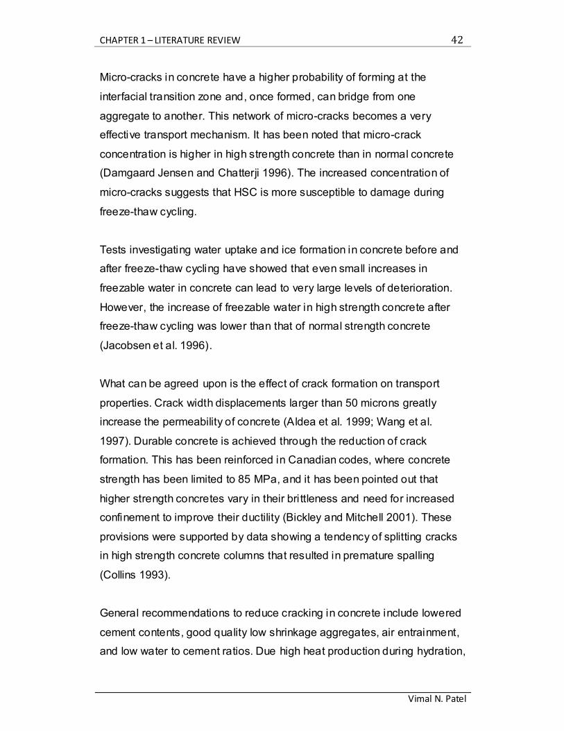
moisture and time. The following diagram illustrates typical absorption
curves for materials tested under different wetting regimes.
Figure 14: Cumulative absorption i(t) through various wetting regimes
Source: (Hall 1981)
Following its introduction, sorptivity testing was more fully investigated and
conditions were set in place to ensure that the absorption relationship
would accurately describe the kinetics of capillary absorption. The four
conditions are:
1) Material homogeneity: the material must be homogeneous over the
scale of the penetration distance
2) Sample geometry: the capillary absorption flow must be normal to
the inflow face and should not converge or diverge
3) Water exposure: water must be freely available at the inflow surface

CHAPTER 1 – LITERATURE REVIEW 45
Vimal N. Patel
4) Test procedure: gravitational effects must not be apparent in the
absorption process
With these conditions and further investigation it was also noted that a
small initial value was often present at t=0. It has been accepted that this
was due to the initial rapid filling of open surface pores on the side faces of
the test specimens (Hall and Tse 1986). To account for this Hall,
introduced an initial value constant A into the relationship to give the
following:
i(t) = S t0.5 + A
With further development of the relationship, it was shown that sorptivity
was a precise quantity that could be measured rapidly and with repeatable
results (Hall and Tse 1986).
1.6.2 Water movement in concrete
In the late 1980’s, sorptivity was used to describe the transport properties
of concrete. Hardened concrete paste, consisting of cement, aggregates
and voids, is rarely saturated in building materials. Often, permeability was
used as a surrogate to durability but this is not entirely accurate.
Permeability relates the movement of moisture through a saturated porous
medium under a pressure gradient. The existence of a concrete structure
under such conditions is considered highly unlikely and so sorptivity
becomes a more accurate characteristic to describe the durability of a
concrete structure.
In contrast to fully saturated materials, where capillary forces are absent,
capillary absorption becomes the primary cause of liquid ingress into
concrete structures. In above-ground structures, the sun and wind dry the
exposed region of concrete while the core remains at a higher degree of
saturation. This differential in saturation creates capillary forces that
become the dominant transport mechanism (McCarter 1993).

CHAPTER 1 – LITERATURE REVIEW 46
Vimal N. Patel
Sorptivity testing on concrete was shown to be sensitive to compaction.
Prolonged ramming of specimens increased bulk density and decreased
porosity. With prolonged ramming, sorptivity plots exhibited a curvature.
This finding brought forward the concept that elimination or reduction of
large pores created this non-linearity (Hall and Raymond Yau 1987).
Application of the sorptivity test to concrete became more important as
there was a worldwide concern about the poor durability of concrete
structures, the most dominant form of deterioration being the corrosion of
steel reinforcement due to the ingress of moisture through the surface skin
of concrete. Sorptivity has been shown to be sensitive to the quality of the
cover skin of concrete members and has proven effective in revealing poor
placing and finishing techniques in the field (McCarter 1993). Further
support was given to sorptivity testing as it was discovered that testing
was also sensitive to the depth of concrete. Specimens that were tested at
different depths for sorptivity gave different results , which could be
indicative of signs of segregation or bleeding due to poor construction
practices (Khatib and Mangat 1995). Figure 15 shows the increased
absorption at the trowelled surface of the specimen.

CHAPTER 1 – LITERATURE REVIEW 47
Vimal N. Patel
Figure 15: Absorption curves relative to depth of exposure surface
Source: (Khatib and Mangat 1995)
By the mid 1990’s, it was generally accepted that good quality concrete
was represented by low sorptivity values and extensive work had been
done on the influence of various factors on water sorptivity. It was shown
that the quality of concrete increased with curing time, and that it varied
based on the source and type of material used. The use of admixtures and
the source of Portland cement also had a large influence on the quality of
concrete described by sorptivity testing (Ho and Chirgwin 1996).
1.6.3 Absorption Tests
In response to the notion that absorption properties provide the most
useful data in relation to the durability of concrete structures and other
building materials, various tests were developed to study absorption
properties; the two most common being the Initial Surface Absorption Test
(ISAT) and the Covercrete Absorption Test (CAT).
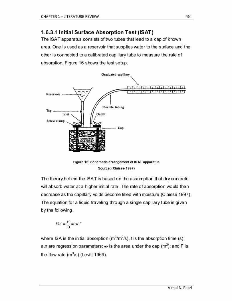
CHAPTER 1 – LITERATURE REVIEW 48
Vimal N. Patel
1.6.3.1 Initial Surface Absorption Test (ISAT)
The ISAT apparatus consists of two tubes that lead to a cap of known
area. One is used as a reservoir that supplies water to the surface and the
other is connected to a calibrated capillary tube to measure the rate of
absorption. Figure 16 shows the test setup.
Figure 16: Schematic arrangement of ISAT apparatus
Source: (Claisse 1997)
The theory behind the ISAT is based on the assumption that dry concrete
will absorb water at a higher initial rate. The rate of absorption would then
decrease as the capillary voids become filled with moisture (Claisse 1997).
The equation for a liquid traveling through a single capillary tube is given
by the following.
ISAF
at n
where ISA is the initial absorption (m3/m2/s), t is the absorption time (s);
a,n are regression parameters; is the area under the cap (m2); and F is
the flow rate (m3/s) (Levitt 1969).
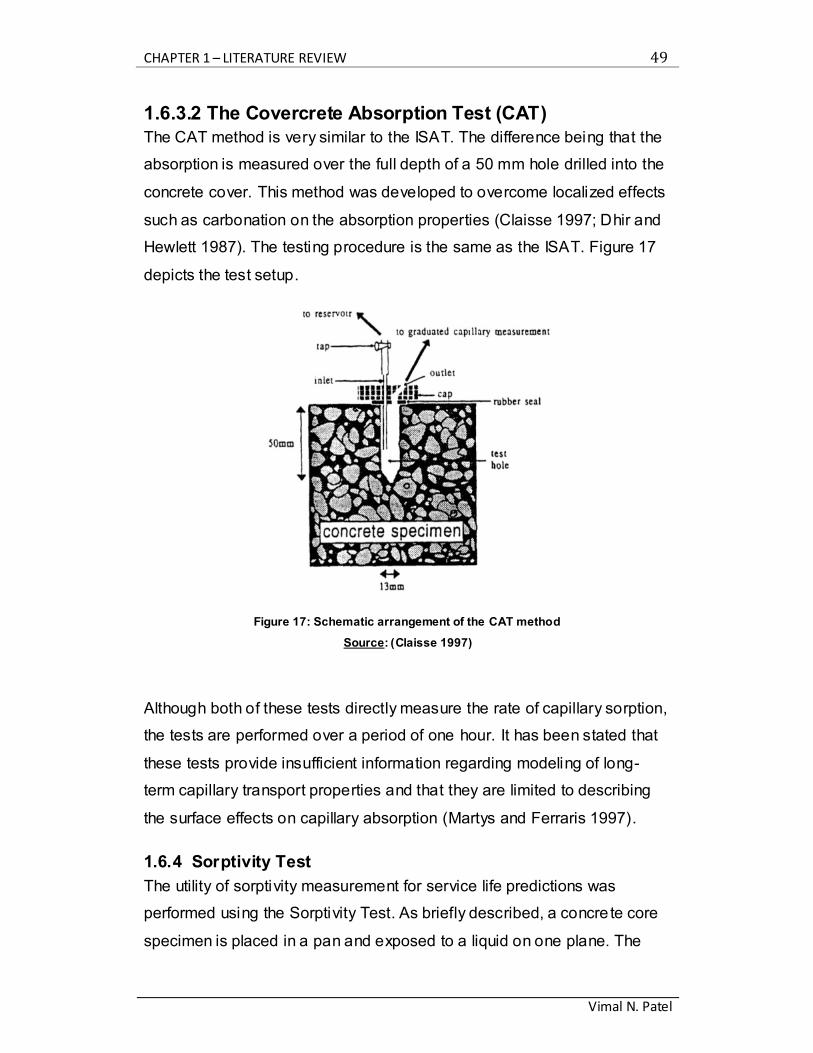
CHAPTER 1 – LITERATURE REVIEW 49
Vimal N. Patel
1.6.3.2 The Covercrete Absorption Test (CAT)
The CAT method is very similar to the ISAT. The difference being that the
absorption is measured over the full depth of a 50 mm hole drilled into the
concrete cover. This method was developed to overcome localized effects
such as carbonation on the absorption properties (Claisse 1997; Dhir and
Hewlett 1987). The testing procedure is the same as the ISAT. Figure 17
depicts the test setup.
Figure 17: Schematic arrangement of the CAT method
Source: (Claisse 1997)
Although both of these tests directly measure the rate of capillary sorption,
the tests are performed over a period of one hour. It has been stated that
these tests provide insufficient information regarding modeling of long-
term capillary transport properties and that they are limited to describing
the surface effects on capillary absorption (Martys and Ferraris 1997).
1.6.4 Sorptivity Test
The utility of sorptivity measurement for service life predictions was
performed using the Sorptivity Test. As briefly described, a concre te core
specimen is placed in a pan and exposed to a liquid on one plane. The
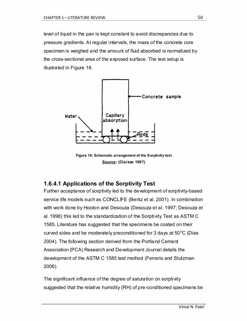
CHAPTER 1 – LITERATURE REVIEW 50
Vimal N. Patel
level of liquid in the pan is kept constant to avoid discrepancies due to
pressure gradients. At regular intervals, the mass of the concrete core
specimen is weighed and the amount of fluid absorbed is normalized by
the cross-sectional area of the exposed surface. The test setup is
illustrated in Figure 18.
Figure 18: Schematic arrangement of the Sorptivity test
Source: (Claisse 1997)
1.6.4.1 Applications of the Sorptivity Test
Further acceptance of sorptivity led to the development of sorptivity-based
service life models such as CONCLIFE (Bentz et al. 2001). In combination
with work done by Hooton and Desouza (Desouza et al. 1997; Desouza et
al. 1998) this led to the standardization of the Sorptivity Test as ASTM C
1585. Literature has suggested that the specimens be coated on their
curved sides and be moderately preconditioned for 3 days at 50oC (Dias
2004). The following section derived from the Portland Cement
Association (PCA) Research and Development Journal details the
development of the ASTM C 1585 test method (Ferraris and Stutzman
2006).
The significant influence of the degree of saturation on sorptivity
suggested that the relative humidity (RH) of pre-conditioned specimens be

CHAPTER 1 – LITERATURE REVIEW 51
Vimal N. Patel
around 60% to emulate field conditions, this RH should be uniformly
attainable across all specimens as quickly as possible and without the use
of sophisticated instruments to ensure a wide range of applications. To
achieve these conditions, specimens needed to be placed in an
environmental chamber at 80% RH and 50oC and then placed into sealed
containers for at least 15 days. The time required in the environmental
chamber was measured by monitoring the RH of concrete specimens in
the environmental chamber at different time intervals (T1: no time, T2: 1
days, T3: 2 days, etc.), as can be seen in Figure 19. After T3 (2 days), the
water content in the specimens was considered uniform throughout the
specimens.
Figure 19: RH achieved after various periods of pre-conditionings in the environmental
chamber at 50oC and 80% RH. The error bars represent one standard deviation
Source: (Ferraris and Stutzman 2006)
The time required for specimens to reach equilibrium after being removed
from the environmental chamber and placed in sealed containers was then
determined. The RH inside the sealed containers was monitored for 30
days and the results in Figure 20 were obtained.
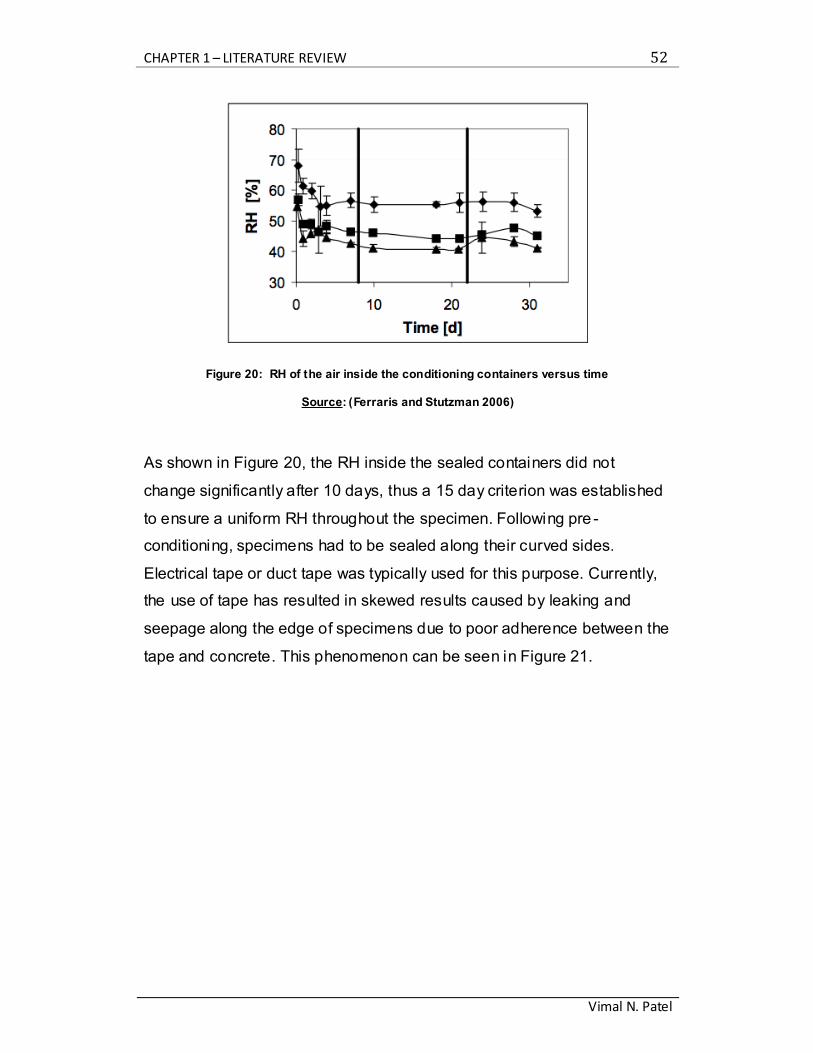
CHAPTER 1 – LITERATURE REVIEW 52
Vimal N. Patel
Figure 20: RH of the air inside the conditioning containers versus time
Source: (Ferraris and Stutzman 2006)
As shown in Figure 20, the RH inside the sealed containers did not
change significantly after 10 days, thus a 15 day criterion was established
to ensure a uniform RH throughout the specimen. Following pre -
conditioning, specimens had to be sealed along their curved sides.
Electrical tape or duct tape was typically used for this purpose. Currently,
the use of tape has resulted in skewed results caused by leaking and
seepage along the edge of specimens due to poor adherence between the
tape and concrete. This phenomenon can be seen in Figure 21.

CHAPTER 1 – LITERATURE REVIEW 53
Vimal N. Patel
Figure 21: Water leak between the tape and specimen sides
Source: (Ferraris and Stutzman 2006)
1.6.4.2 Boundary Conditions of Sorptivity Test
The test setup for sorptivity has been shown to be sensitive to boundary
conditions. Sorptivity testing based on ASTM C 158504 consists of
subjecting a disc-shaped concrete specimen (100 mm in diameter and 50
mm in thickness) to one-sided exposure to water. In order to ensure a uni-
directional flow, the remaining surfaces of the specimen that are not
immersed must be sealed appropriately with a suitable material. After
scanning the literature, it became evident that a wide variability of
sorptivity values exists, depending on the choice of sealant. These include
electrical insulation tape, grease, bituminous paint, and paraffin wax
(Caliskan 2006; Claisse 1997; Gonen and Yazicioglu 2007; Taha 2001).
Sabir (1998) has even suggested a test set-up that does not require
sealant material. The test setup consisted of a continuously monitored
sorptivity test that did not require weight measurements at given intervals.
Rather, the specimen was connected to a balance, which transferred data
electronically to a PC. The test setup is seen in Figure 22.
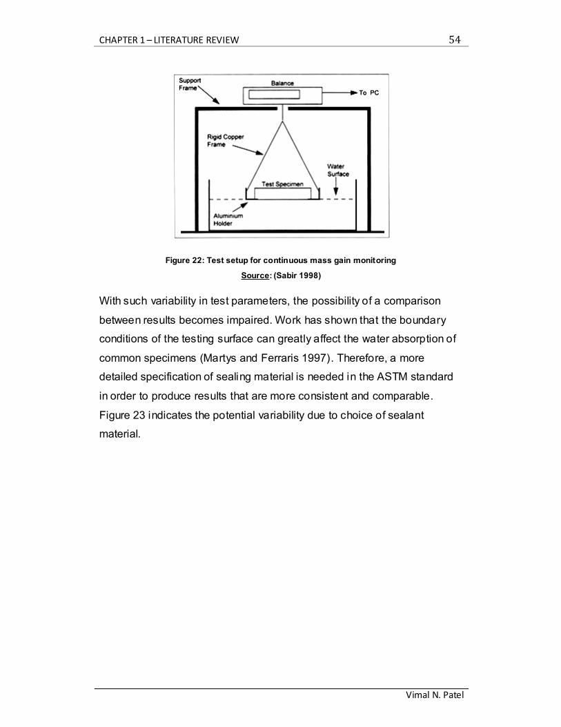
CHAPTER 1 – LITERATURE REVIEW 54
Vimal N. Patel
Figure 22: Test setup for continuous mass gain monitoring
Source: (Sabir 1998)
With such variability in test parameters, the possibility of a comparison
between results becomes impaired. Work has shown that the boundary
conditions of the testing surface can greatly affect the water absorption of
common specimens (Martys and Ferraris 1997). Therefore, a more
detailed specification of sealing material is needed in the ASTM standard
in order to produce results that are more consistent and comparable.
Figure 23 indicates the potential variability due to choice of sealant
material.

CHAPTER 1 – LITERATURE REVIEW 55
Vimal N. Patel
Figure 23: Sorptivity relative to type of sealant material
Source: (Martys and Ferraris 1997)
Hall (1986) suggested the modification to the absorption relationship by
adding an initial value (A), given below.
i(t) = S t0.5 + A
The addition of the constant was designed to take into account the initial
absorption due to the non-exposed side faces of the specimen. Even with
this constant, further work should be pursued to determine an adequate
sealant material that would eliminate the need for an initial absorption
coefficient as well as to increase the consistency of standardized testing.
Despite these weaknesses, development of the sorptivity test continued
and has made its move to in-situ testing. Further investigation of
absorption through field-testing provided consistent and meaningful
results. Curing techniques could be distinguished as either effective or
ineffective with field tests. As well, the moisture content of the cover
concrete could be determined in-situ (Desouza et al. 1998). Figure 24
shows a field test derived from the ISAT.
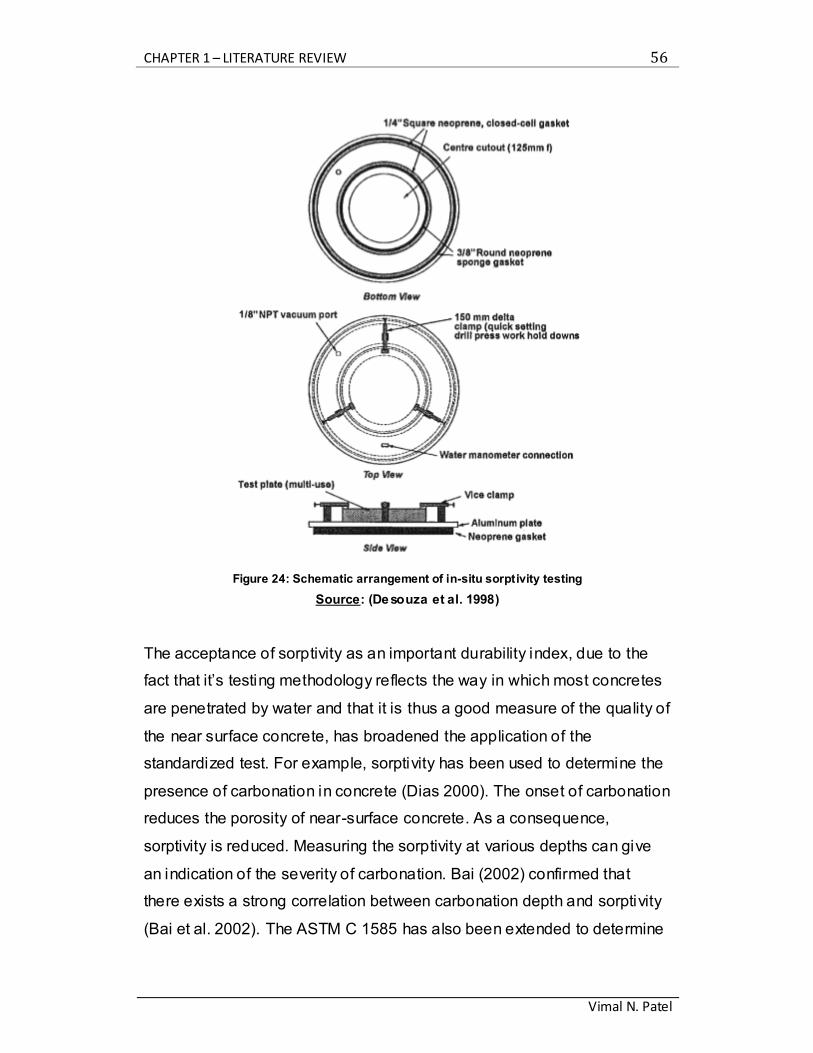
CHAPTER 1 – LITERATURE REVIEW 56
Vimal N. Patel
Figure 24: Schematic arrangement of in-situ sorptivity testing
Source: (Desouza et al. 1998)
The acceptance of sorptivity as an important durability index, due to the
fact that it’s testing methodology reflects the way in which most concretes
are penetrated by water and that it is thus a good measure of the quality of
the near surface concrete, has broadened the application of the
standardized test. For example, sorptivity has been used to determine the
presence of carbonation in concrete (Dias 2000). The onset of carbonation
reduces the porosity of near-surface concrete. As a consequence,
sorptivity is reduced. Measuring the sorptivity at various depths can give
an indication of the severity of carbonation. Bai (2002) confirmed that
there exists a strong correlation between carbonation depth and sorptivity
(Bai et al. 2002). The ASTM C 1585 has also been extended to determine
CHAPTER 1 – LITERATURE REVIEW 57
Vimal N. Patel
the effects of compaction on the durability of the concrete (Gonen and
Yazicioglu 2007). Various applications of the standard have also included
determining water absorption at 28 and 56 days to study the continuation
of cement hydration in concrete (El-Dieb 2007). As well, the standard has
been applied to evaluate the effectiveness of fly ash and slag in lowering
the transport properties in concretes (Radlinski et al. 2007).
It has been shown that the dominant characteristics in concrete
degradation are its near-surface properties (Basheer et al. 2001), thus
tests methods characterizing the surface zone of concrete, such as the
ASTM C 1585, become very important .
Since standardization, the sorptivity test has been used to formulate
performance specifications that would allow the optimization of concrete
mixture designs (Obla 2006).
1.6.4.3 Sorptivity and Self-Compacting Concrete
With the development of self-compacting concrete (SCC) much of the
research has focused the fresh properties of the mix; such as flow,
resistance to segregation and bleeding, and stability. However, little work
has been done assessing the durability characteristics of SCC in
comparison to normal vibrated concrete. With respect to sorptivity, an
SCC contains a combination of superplasticizers and a viscosity-modifying
agent (VMA). It has been shown that the presence of the VMA’s fine
powder material may reduce the absorption of SCC (Zhu and Bartos
2003). The fact that an SCC mix will have a more homogeneous structure
and denser interfacial transition zone (ITZ) in comparison to a normal
vibrated concrete of similar strength can be the reason for its low
sorptivity. Although the ITZ has a higher overall porosity, the lack of pore
continuity reduces its absorption properties (Sabir 1998). Current literature
suggests that SCC exhibits low absorption values compared to normal
concrete due to its denser structure, which is achieved through better
CHAPTER 1 – LITERATURE REVIEW 58
Vimal N. Patel
hydration and enhanced rheological properties (Caliskan 2006; Persson
2001). Some work has assessed durability properties of SCC vs. vibrated
concrete; showing that durability properties of SCC could be regarded as
equivalent based on tests such as mercury intrusion porosimetry, water
absorption, and chloride diffusion (Assie et al. 2007). However, there is
limited knowledge on the absorption of SCC in reference to normal
concrete under stress or after freeze-thaw cycling. These stress conditions
can change the pore structure of the concrete and induce continuity in the
ITZ, which would greatly affect sorptivity. It should also be mentioned that
such conditions better simulate field conditions.
CHAPTER 2 – EXPERIMENTAL PROGRAM 59
Vimal N. Patel
CHAPTER 2 – EXPERIMENTAL PROGRAM
2.1 Material Preparation
The sorptivity experiment testing was guided by the ASTM Standard Test
Method for Measurement of Rate of Absorption of Water by Hydraulic-
Cement Concretes (ASTM C 1585-04). The following section describe in
more detail the material preparation, test specimens, equipment and
experimental procedure used in this research.
2.1.1 Mixing Equipment and Set Up
- Barrel Mixer
- Vibratory Table
- 4‖x 8‖Cylinder Moulds
- Slump Cone
- Tamping Rod
- Air Pressure Meter
- Slump Flow Board
- Compressive Strength Test Apparatus
- Freeze-Thaw Chamber
2.1.2 Materials
To determine the influence of material properties on the rate of absorption,
three different concrete mixes were cast. Mix A consisted of a high
strength concrete without air entrainment. Mix B consisted of a high
strength concrete with air entrainment. Finally, Mix C was a self-
consolidating concrete (SCC). Details of the mixture designs are shown in
Table 2.
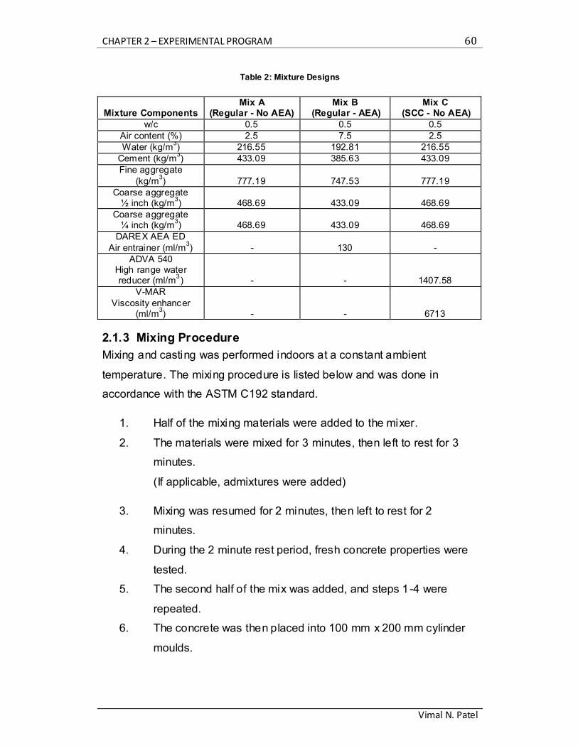
CHAPTER 2 – EXPERIMENTAL PROGRAM 60
Vimal N. Patel
Table 2: Mixture Designs
Mixture Components Mix A
(Regular - No AEA) Mix B
(Regular - AEA) Mix C
(SCC - No AEA)
w/c 0.5 0.5 0.5
Air content (%) 2.5 7.5 2.5
Water (kg/m3) 216.55 192.81 216.55
Cement (kg/m3) 433.09 385.63 433.09
Fine aggregate
(kg/m3) 777.19 747.53 777.19
Coarse aggregate ½ inch (kg/m
3) 468.69 433.09 468.69
Coarse aggregate ¼ inch (kg/m
3) 468.69 433.09 468.69
DAREX AEA ED
Air entrainer (ml/m3) - 130 -
ADVA 540 High range water reducer (ml/m
3) - - 1407.58
V-MAR
Viscosity enhancer (ml/m
3) - - 6713
2.1.3 Mixing Procedure
Mixing and casting was performed indoors at a constant ambient
temperature. The mixing procedure is listed below and was done in
accordance with the ASTM C192 standard.
1. Half of the mixing materials were added to the mixer.
2. The materials were mixed for 3 minutes, then left to rest for 3
minutes.
(If applicable, admixtures were added)
3. Mixing was resumed for 2 minutes, then left to rest for 2
minutes.
4. During the 2 minute rest period, fresh concrete properties were
tested.
5. The second half of the mix was added, and steps 1-4 were
repeated.
6. The concrete was then placed into 100 mm x 200 mm cylinder
moulds.
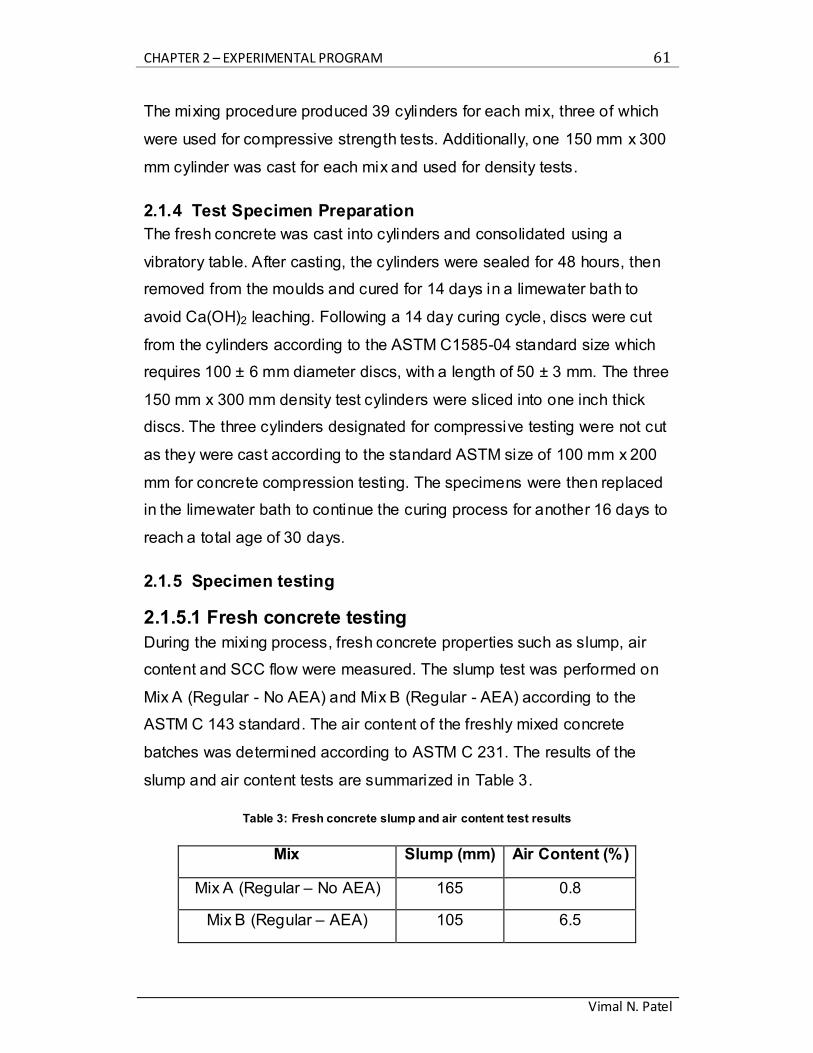
CHAPTER 2 – EXPERIMENTAL PROGRAM 61
Vimal N. Patel
The mixing procedure produced 39 cylinders for each mix, three of which
were used for compressive strength tests. Additionally, one 150 mm x 300
mm cylinder was cast for each mix and used for density tests.
2.1.4 Test Specimen Preparation
The fresh concrete was cast into cylinders and consolidated using a
vibratory table. After casting, the cylinders were sealed for 48 hours, then
removed from the moulds and cured for 14 days in a limewater bath to
avoid Ca(OH)2 leaching. Following a 14 day curing cycle, discs were cut
from the cylinders according to the ASTM C1585-04 standard size which
requires 100 ± 6 mm diameter discs, with a length of 50 ± 3 mm. The three
150 mm x 300 mm density test cylinders were sliced into one inch thick
discs. The three cylinders designated for compressive testing were not cut
as they were cast according to the standard ASTM size of 100 mm x 200
mm for concrete compression testing. The specimens were then replaced
in the limewater bath to continue the curing process for another 16 days to
reach a total age of 30 days.
2.1.5 Specimen testing
2.1.5.1 Fresh concrete testing
During the mixing process, fresh concrete properties such as slump, air
content and SCC flow were measured. The slump test was performed on
Mix A (Regular - No AEA) and Mix B (Regular - AEA) according to the
ASTM C 143 standard. The air content of the freshly mixed concrete
batches was determined according to ASTM C 231. The results of the
slump and air content tests are summarized in Table 3.
Table 3: Fresh concrete slump and air content test results
Mix Slump (mm) Air Content (%)
Mix A (Regular – No AEA) 165 0.8
Mix B (Regular – AEA) 105 6.5
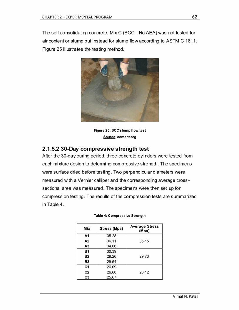
CHAPTER 2 – EXPERIMENTAL PROGRAM 62
Vimal N. Patel
The self-consolidating concrete, Mix C (SCC - No AEA) was not tested for
air content or slump but instead for slump flow according to ASTM C 1611.
Figure 25 illustrates the testing method.
Figure 25: SCC slump flow test
Source: cement.org
2.1.5.2 30-Day compressive strength test
After the 30-day curing period, three concrete cylinders were tested from
each mixture design to determine compressive strength. The specimens
were surface dried before testing. Two perpendicular diameters were
measured with a Vernier calliper and the corresponding average cross -
sectional area was measured. The specimens were then set up for
compression testing. The results of the compression tests are summarized
in Table 4.
Table 4: Compressive Strength
Mix Stress (Mpa) Average Stress
(Mpa)
A1 35.28
A2 36.11 35.15
A3 34.06
B1 30.39
B2 29.26 29.73
B3 29.54
C1 26.09
C2 26.60 26.12
C3 25.67
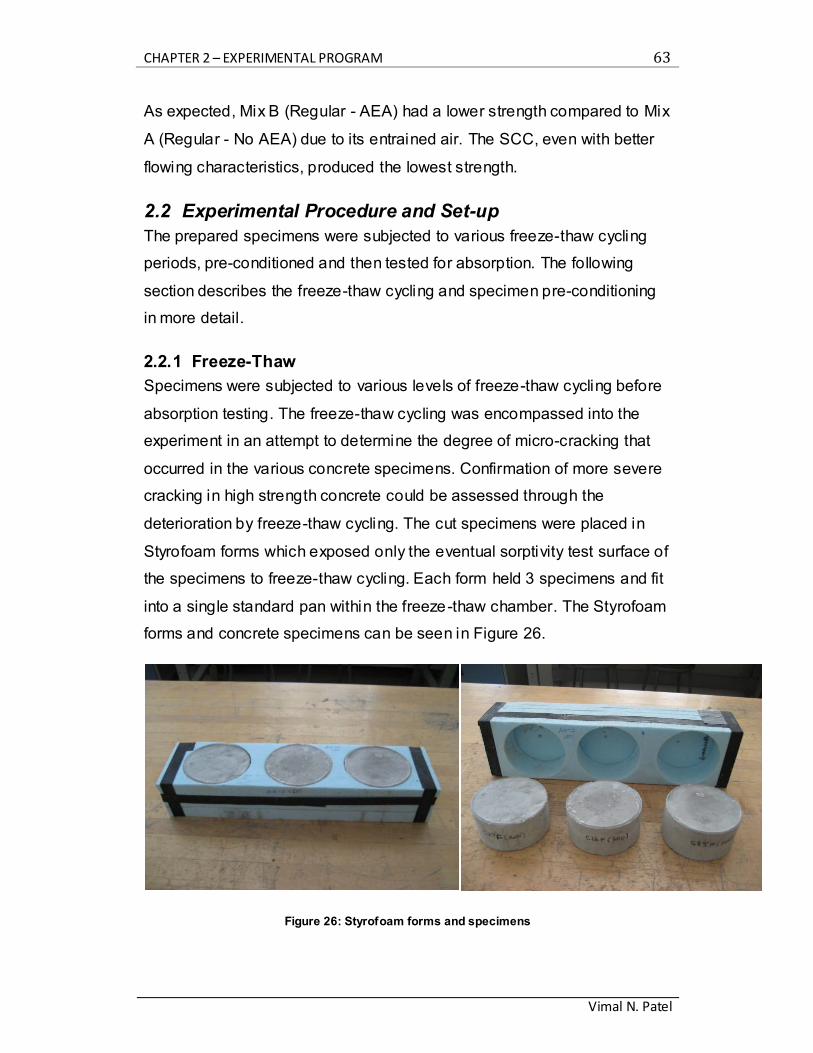
CHAPTER 2 – EXPERIMENTAL PROGRAM 63
Vimal N. Patel
As expected, Mix B (Regular - AEA) had a lower strength compared to Mix
A (Regular - No AEA) due to its entrained air. The SCC, even with better
flowing characteristics, produced the lowest strength.
2.2 Experimental Procedure and Set-up
The prepared specimens were subjected to various freeze-thaw cycling
periods, pre-conditioned and then tested for absorption. The following
section describes the freeze-thaw cycling and specimen pre-conditioning
in more detail.
2.2.1 Freeze-Thaw
Specimens were subjected to various levels of freeze-thaw cycling before
absorption testing. The freeze-thaw cycling was encompassed into the
experiment in an attempt to determine the degree of micro-cracking that
occurred in the various concrete specimens. Confirmation of more severe
cracking in high strength concrete could be assessed through the
deterioration by freeze-thaw cycling. The cut specimens were placed in
Styrofoam forms which exposed only the eventual sorptivity test surface of
the specimens to freeze-thaw cycling. Each form held 3 specimens and fit
into a single standard pan within the freeze-thaw chamber. The Styrofoam
forms and concrete specimens can be seen in Figure 26.
Figure 26: Styrofoam forms and specimens
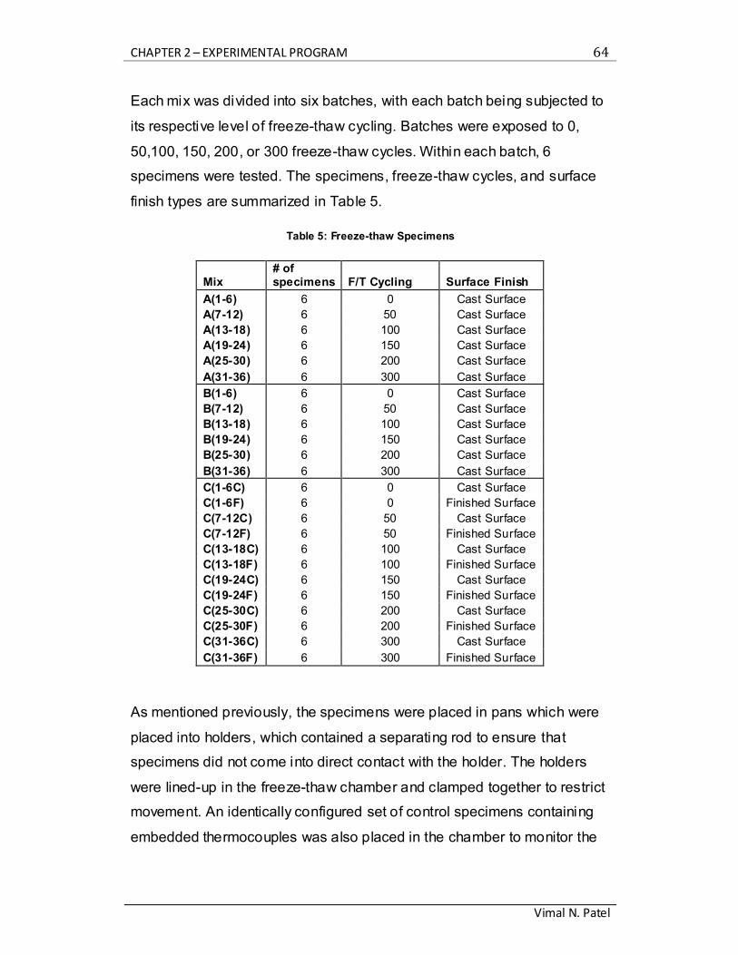
CHAPTER 2 – EXPERIMENTAL PROGRAM 64
Vimal N. Patel
Each mix was divided into six batches, with each batch being subjected to
its respective level of freeze-thaw cycling. Batches were exposed to 0,
50,100, 150, 200, or 300 freeze-thaw cycles. Within each batch, 6
specimens were tested. The specimens, freeze-thaw cycles, and surface
finish types are summarized in Table 5.
Table 5: Freeze-thaw Specimens
Mix # of specimens F/T Cycling Surface Finish
A(1-6) 6 0 Cast Surface
A(7-12) 6 50 Cast Surface
A(13-18) 6 100 Cast Surface
A(19-24) 6 150 Cast Surface
A(25-30) 6 200 Cast Surface
A(31-36) 6 300 Cast Surface
B(1-6) 6 0 Cast Surface
B(7-12) 6 50 Cast Surface
B(13-18) 6 100 Cast Surface
B(19-24) 6 150 Cast Surface
B(25-30) 6 200 Cast Surface
B(31-36) 6 300 Cast Surface
C(1-6C) 6 0 Cast Surface
C(1-6F) 6 0 Finished Surface
C(7-12C) 6 50 Cast Surface
C(7-12F) 6 50 Finished Surface
C(13-18C) 6 100 Cast Surface
C(13-18F) 6 100 Finished Surface
C(19-24C) 6 150 Cast Surface
C(19-24F) 6 150 Finished Surface
C(25-30C) 6 200 Cast Surface
C(25-30F) 6 200 Finished Surface
C(31-36C) 6 300 Cast Surface
C(31-36F) 6 300 Finished Surface
As mentioned previously, the specimens were placed in pans which were
placed into holders, which contained a separating rod to ensure that
specimens did not come into direct contact with the holder. The holders
were lined-up in the freeze-thaw chamber and clamped together to restrict
movement. An identically configured set of control specimens containing
embedded thermocouples was also placed in the chamber to monitor the
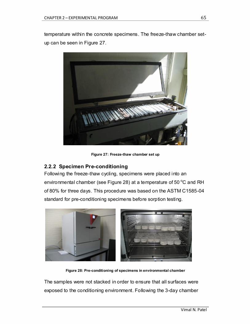
CHAPTER 2 – EXPERIMENTAL PROGRAM 65
Vimal N. Patel
temperature within the concrete specimens. The freeze-thaw chamber set-
up can be seen in Figure 27.
Figure 27: Freeze-thaw chamber set up
2.2.2 Specimen Pre-conditioning
Following the freeze-thaw cycling, specimens were placed into an
environmental chamber (see Figure 28) at a temperature of 50 oC and RH
of 80% for three days. This procedure was based on the ASTM C1585-04
standard for pre-conditioning specimens before sorption testing.
Figure 28: Pre-conditioning of specimens in environmental chamber
The samples were not stacked in order to ensure that all surfaces were
exposed to the conditioning environment. Following the 3-day chamber
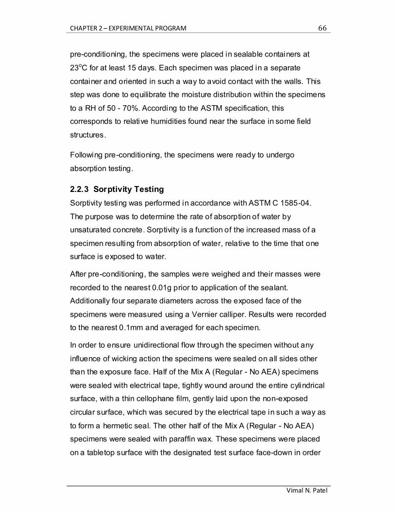
CHAPTER 2 – EXPERIMENTAL PROGRAM 66
Vimal N. Patel
pre-conditioning, the specimens were placed in sealable containers at
23oC for at least 15 days. Each specimen was placed in a separate
container and oriented in such a way to avoid contact with the walls. This
step was done to equilibrate the moisture distribution within the specimens
to a RH of 50 - 70%. According to the ASTM specification, this
corresponds to relative humidities found near the surface in some field
structures.
Following pre-conditioning, the specimens were ready to undergo
absorption testing.
2.2.3 Sorptivity Testing
Sorptivity testing was performed in accordance with ASTM C 1585-04.
The purpose was to determine the rate of absorption of water by
unsaturated concrete. Sorptivity is a function of the increased mass of a
specimen resulting from absorption of water, relative to the time that one
surface is exposed to water.
After pre-conditioning, the samples were weighed and their masses were
recorded to the nearest 0.01g prior to application of the sealant.
Additionally four separate diameters across the exposed face of the
specimens were measured using a Vernier calliper. Results were recorded
to the nearest 0.1mm and averaged for each specimen.
In order to ensure unidirectional flow through the specimen without any
influence of wicking action the specimens were sealed on all sides other
than the exposure face. Half of the Mix A (Regular - No AEA) specimens
were sealed with electrical tape, tightly wound around the entire cylindrical
surface, with a thin cellophane film, gently laid upon the non-exposed
circular surface, which was secured by the electrical tape in such a way as
to form a hermetic seal. The other half of the Mix A (Regular - No AEA)
specimens were sealed with paraffin wax. These specimens were placed
on a tabletop surface with the designated test surface face-down in order
CHAPTER 2 – EXPERIMENTAL PROGRAM 67
Vimal N. Patel
to keep it free of wax sealant. Melted wax was then applied with a brush to
the remaining surfaces. Care was taken to ensure that the all
imperfections, pits, and small dimples were filled with melted wax. The
paraffin was allowed to cool, forming a watertight and airtight seal. A
second layer of wax sealant was applied in the same manner to ensure
that a proper seal was achieved. Both sealing procedures as outlined
above were repeated for Mixes B (Regular - AEA), Mix CC (SCC Cast
Face – No AEA) and Mix CF (SCC Finished Face – No AEA).
The masses of the prepared specimens were measured and recorded to
the nearest 0.01g once more. These values formed the initial mass value
set for absorption calculations. A support consisting of fibreglass fi lter
material was placed in the bottom of each container to ensure that
exposure to water was even across the exposed surface. The specimen
was placed atop this support and the container was gently filled with tap
water until it reached a level approximately 1 to 3 mm above the level of
the exposed surface. The tap water used in this experiment was dyed with
food coloring in an attempt to illustrate the flow path of absorbed water.
The pressure head resulting from the 1 to 3 mm of immersion can be
considered negligible. In this experiment, absorption was to be the result
of capillary rise only. This simulates the behaviour of most concrete
structures in the field. A digital timer was initiated from the moment the
exposed surface came into contact with the water.
The specimen masses were recorded at intervals of 60 seconds, 5, 10, 20,
20, 30, and 60 minutes, 2, 3, 4, 5, and 6 hours and 1, 2, 3, 4, 5, 6, 7 and 8
days in accordance with the ASTM standard. Each specimen was quickly
removed from the water, had its test surface patted with a paper towel to
remove excess water and was then placed on the electronic scale upside-
down such that the exposed face never came in contact with the scale,
which could potentially allow water to be lost from the specimen.
CHAPTER 2 – EXPERIMENTAL PROGRAM 68
Vimal N. Patel
Water levels in the container were checked daily to ensure that the 1 to 3
mm immersion range was maintained at all times throughout the
experiment.
The absorption, I, was calculated as the change in mass divided by the
product of the cross-sectional area of the test specimen (a) and the
density of water (d). In accordance with the ASTM Standard, for the
purpose of the test, the temperature dependency of the density of water
was neglected and a value of 0.001 g/mm3 is used. The units of I are mm.
The absorption values were then plotted against time to produce
absorption curves. The rate of change of the absorption curves at various
times was called sorptivity; S. Sorptivity values were then plotted against
time to investigate changes in the rate of absorption.
2.2.4 Density Testing
To investigate whether significant segregation had occurred during casting
of the specimens, the density, percent-absorption, and percent-voids in
the hardened concrete were determined at incremental depths, in
accordance with ASTM Standard C 642 - 97. For this test, 25-mm thick
cylindrical slices were cut from the 300 mm x 600 mm concrete cylinders,
which had been stored at room temperature following the standard curing
regime. Four mass values were required for each sample to calculate the
density, absorption and voids percentage (see Table 5); oven-dry mass
(A), saturated mass after immersion (B) and after boiling (C), and
immersed apparent mass (D).
First, the oven-dry mass of each specimen was obtained after several
drying cycles. To obtain this value, each specimen was oven-dried at a
temperature of 105 oC for not less than 24 hours, allowed to cool under
ambient conditions, and then weighed and having its mass recorded. This
cycle was repeated until the percent-change of mass between two

CHAPTER 2 – EXPERIMENTAL PROGRAM 69
Vimal N. Patel
successive readings was less than 0.5%. The final, lowest, value was
retained as the oven-dry mass.
Second, the saturated mass after immersion was measured after cyclic
immersion cycles. The specimens were immersed in water at
approximately 21 oC for not less than 48 hours before being removed,
surface-dried and weighed. Their masses were measured and recorded.
Similarly to the oven-dry mass, this process was repeated until two
successive values fell within a 0.5% percent change. The final, highest
value was retained as the saturated mass after immersion.
Third, the saturated mass after boiling was measured by placing the
specimens in a metal receptacle suitable for heating over a hotplate,
immersing the specimens in water and bringing this water to boil for five
hours. The specimens remained immersed as they cooled by natural heat
loss under ambient conditions unti l they reached room temperature. A
maximum of 14 hours of cooling was allowed. At this point, the specimens
were surface-dried and their masses were measured and recorded.
Finally, after drying, immersion and boiling, the apparent mass was
determined for each specimen. The specimen was suspended from the
base hook of an electronic balance and immersed in a bucket of water.
The mass of the buoyant specimen was recorded as the apparent mass.
By using these four mass values the results of the density test, found in
Appendix A, were obtained according to calculations outlined in the ASTM
C 642 – 97 standard. Figure 29 illustrates the permeable pore space
results of the ASTM C 642 – 97 standard over the depth of all mixes.
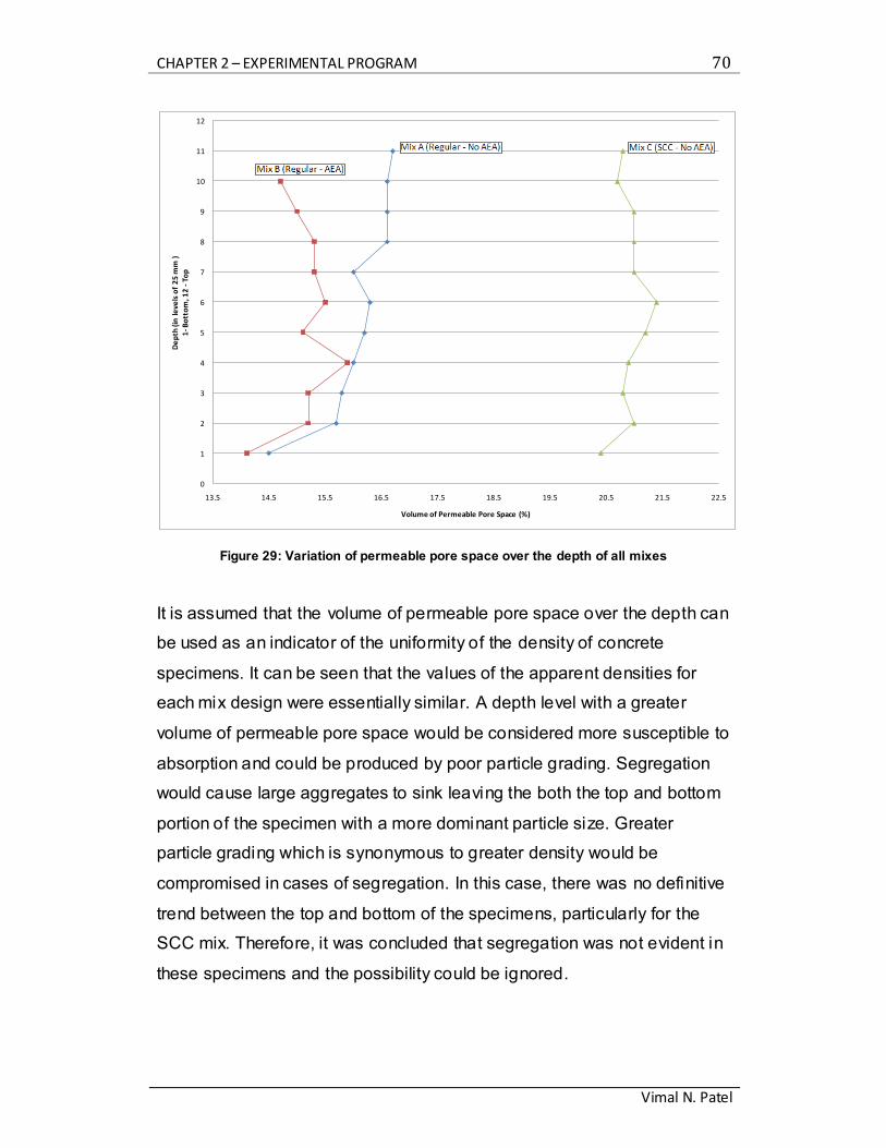
CHAPTER 2 – EXPERIMENTAL PROGRAM 70
Vimal N. Patel
Figure 29: Variation of permeable pore space over the depth of all mixes
It is assumed that the volume of permeable pore space over the depth can
be used as an indicator of the uniformity of the density of concrete
specimens. It can be seen that the values of the apparent densities for
each mix design were essentially similar. A depth level with a greater
volume of permeable pore space would be considered more susceptible to
absorption and could be produced by poor particle grading. Segregation
would cause large aggregates to sink leaving the both the top and bottom
portion of the specimen with a more dominant particle size. Greater
particle grading which is synonymous to greater density would be
compromised in cases of segregation. In this case, there was no definitive
trend between the top and bottom of the specimens, particularly for the
SCC mix. Therefore, it was concluded that segregation was not evident in
these specimens and the possibility could be ignored.
0
1
2
3
4
5
6
7
8
9
10
11
12
13.5 14.5 15.5 16.5 17.5 18.5 19.5 20.5 21.5 22.5
De
pth
(in
le
vels
of
25
mm
)1
-Bo
tto
m, 1
2 -
Top
Volume of Permeable Pore Space (%)
CHAPTER 3 – RESULTS AND DISCUSSION 71
Vimal N. Patel
CHAPTER 3 – RESULTS AND DISCUSSION
The following chapter consists of an analysis of the data collected from
specimens of a non air-entrained mixture Mix A (Regular - No AEA) the
specimens from an air-entrained mixture Mix B (Regular - AEA), and a
self-consolidating concrete mixture Mix C (SCC - No AEA). As mentioned
in the experimental program all specimens were pre-conditioned to a
relative humidity of 50 to 70% at 23oC before being subjected to freeze-
thaw cycling in the same chamber. Based on the hydraulic pressure
theory, the only parameters thus differentiating the specimens were their
flow properties, rendering the results to be sensitive to the concrete mix in
particular instead of the environment. Secondly, based on Litvan’s theory,
although specimens were not saturated upon introduction to the freeze-
thaw chamber, it was assumed that the onset of cracking would begin at
the initial stages of exposure. Tap water was used during freeze-thaw
cycling, based on the osmotic pressure theory, it should be assumed that
the results obtained would be conservative compared to field conditions
where water has a significantly higher concentration of deleterious
substances.
3.1 Influence of materials on performance of mix design
Several key points regarding the influence of materials and their properties
on the performance of mix designs is outlined in the following section.
Special attention was paid to the effect on air void stability as it was
considered the primary parameter affecting the resistance to freeze-thaw
cycling.
The first parameter of interest was the w/c of the mix designs. Mixes A
(Regular – No AEA), B (Regular - AEA), and C (SCC – No AEA) were
designed with a w/c of 0.50. This ratio was calculated based on the free
water added over the quantity of cement used. It should be noted however
that the addition of superplasticizers and viscosity modifying admixture to
CHAPTER 3 – RESULTS AND DISCUSSION 72
Vimal N. Patel
Mix C (SCC - No AEA) could have increased the w/c ratio to 0.52. This
calculation was based on the assumption that the admixtures had a 99%
water content. As mentioned in Chapter 1, mixes with higher w/c require a
smaller spacing factor in order to achieve an equivalent freeze-thaw
resistance. Noting that Mix C (SCC - No AEA) had no air-entrainment, the
previously published literature suggests that it would perform poorly
compared to other mixes with air entrainment or with lower w/c values. On
the same note, the characteristics of the aggregate influenced the
viscosity of the paste. Finer cement was mentioned as a means to
increase air void stability. The current mix designs were considered not to
have a significant difference in fine aggregate content, which ranged from
747 to 777 kg/m3 of natural sand for all three mixes. Visual observations of
the coarse aggregates in Figure 30 revealed cracking through the
aggregate particles. Based on these observations, it would be
recommended to limit the coarse aggregate size to ¼’’ to help avoid
cracking.
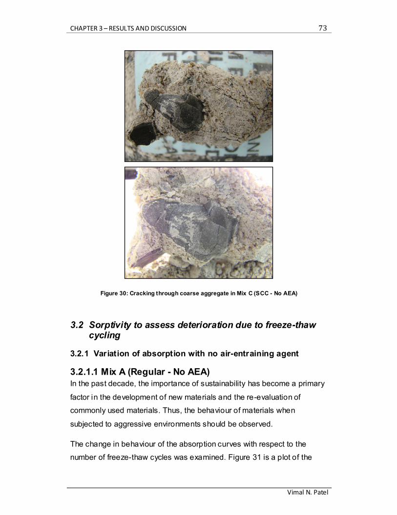
CHAPTER 3 – RESULTS AND DISCUSSION 73
Vimal N. Patel
Figure 30: Cracking through coarse aggregate in Mix C (SCC - No AEA)
3.2 Sorptivity to assess deterioration due to freeze-thaw cycling
3.2.1 Variation of absorption with no air-entraining agent
3.2.1.1 Mix A (Regular - No AEA)
In the past decade, the importance of sustainability has become a primary
factor in the development of new materials and the re-evaluation of
commonly used materials. Thus, the behaviour of materials when
subjected to aggressive environments should be observed.
The change in behaviour of the absorption curves with respect to the
number of freeze-thaw cycles was examined. Figure 31 is a plot of the

CHAPTER 3 – RESULTS AND DISCUSSION 74
Vimal N. Patel
absorption curves of Mix A (Regular - No AEA) for every level of freeze-
thaw cycling. The variation in the curvature of the graphs for every level of
freeze-thaw cycle suggests that behavioural change do in fact occur. As
can be seen in Figure 31, the behaviour of Mix A (Regular - No AEA) at
zero cycles of freeze-thaw (i.e. not exposed to freeze-thaw cycling) greatly
differs from that of samples after 150 cycles. Samples from this mix
subjected to freeze-thaw beyond 150 cycles experienced severe
deterioration and were deemed un-testable.
Figure 31: Effect of freeze-thaw cycling on absorption of Mix A (Regular - No AEA)
The variation in the curvature was characterized by significant changes in
slope. Sample A(150) demonstrated an acute bi-linear behaviour in
comparison to A(0) and A(50), where a more gradual change in slope was
present. The location at which this shift in slope occurred was called the
nick point.
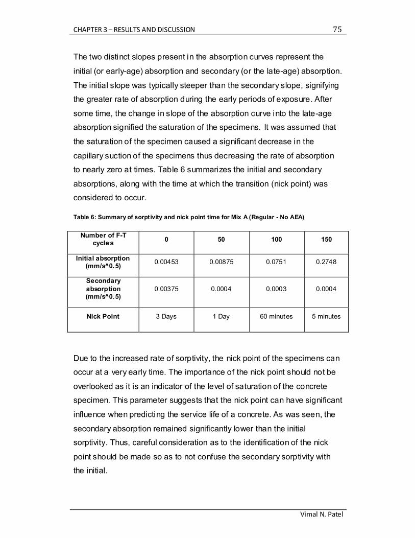
CHAPTER 3 – RESULTS AND DISCUSSION 75
Vimal N. Patel
The two distinct slopes present in the absorption curves represent the
initial (or early-age) absorption and secondary (or the late-age) absorption.
The initial slope was typically steeper than the secondary slope, signifying
the greater rate of absorption during the early periods of exposure. After
some time, the change in slope of the absorption curve into the late-age
absorption signified the saturation of the specimens. It was assumed that
the saturation of the specimen caused a significant decrease in the
capillary suction of the specimens thus decreasing the rate of absorption
to nearly zero at times. Table 6 summarizes the initial and secondary
absorptions, along with the time at which the transition (nick point) was
considered to occur.
Table 6: Summary of sorptivity and nick point time for Mix A (Regular - No AEA)
Number of F-T cycles
0 50 100 150
Initial absorption (mm/s 0.5)
0.00453 0.00875 0.0751 0.2748
Secondary
absorption (mm/s 0.5)
0.00375 0.0004 0.0003 0.0004
Nick Point 3 Days 1 Day 60 minutes 5 minutes
Due to the increased rate of sorptivity, the nick point of the specimens can
occur at a very early time. The importance of the nick point should not be
overlooked as it is an indicator of the level of saturation of the concrete
specimen. This parameter suggests that the nick point can have significant
influence when predicting the service life of a concrete. As was seen, the
secondary absorption remained significantly lower than the initial
sorptivity. Thus, careful consideration as to the identification of the nick
point should be made so as to not confuse the secondary sorptivity with
the initial.

CHAPTER 3 – RESULTS AND DISCUSSION 76
Vimal N. Patel
Figure 32: Effect of F-T cycling on early-age sorptivity of all mixes (0-6 hours)
Figure 33: Effect of F-T cycling on the late-age sorptivity of all mixes (1-8 days)
0
0.05
0.1
0.15
0.2
0.25
0.3
0 50 100 150 200 250 300
Sorp
tivi
ty (
mm
/s^1
/2)
Freeze Thaw Cycles
Mix A (Regular - No AEA)
Mix CC (SCC Cast - No AEA)
Mix CF (SCC Finished - No AEA)Mix B (Regular - AEA)
Specimens no longer testable due to severe damage
0
0.001
0.002
0.003
0.004
0.005
0 50 100 150 200 250 300
sorp
tivi
ty (
mm
/s^1
/2)
Freeze Thaw Cycles
The values for Mix A, CC, and CF after 50 cycles that are circled were assumed values based on sorptivity values with very low
linearity.
Mix CF (SCC Finished - No AEA)
Mix CF (SCC Finished - No AEA)
Mix B (Regular - AEA)
Mix A (regular- No AEA)
Specimens no longer testable due to severe damage

CHAPTER 3 – RESULTS AND DISCUSSION 77
Vimal N. Patel
When data from Table 6 was plotted, it can be seen from Figure 32 that
the rate of initial absorption of Mix A (Regular - No AEA) increased at what
seemed a parabolic rate versus the number of freeze-thaw cycles. The
results suggested that freeze-thaw cycling can have a dramatic effect on
the rate of initial absorption of a concrete mix with no air-entrainment.
Results for Mix CC (SCC Cast – No AEA) and CF (SCC Finished – No
AEA) could not be obtained since the samples were deemed un-testable
due to severe deterioration (it can be assumed that Mix C (SCC - No AEA)
would have similar behavioural traits to Mix A (Regular - No AEA) had it
been testable). Further details about Mix C (SCC - No AEA) have been
outlined in the following section.
3.2.1.2 Mix C (SCC - No AEA)
The same data analysis was done on Mix C (SCC with no AEA) and
resulted in similar results. Although, numerical results were not identical,
the behavioural pattern of absorption curves remained the same for Mix C
(SCC - No AEA) when compared to Mix A (Regular - No AEA). The plot of
the data can be seen in Figure 34.
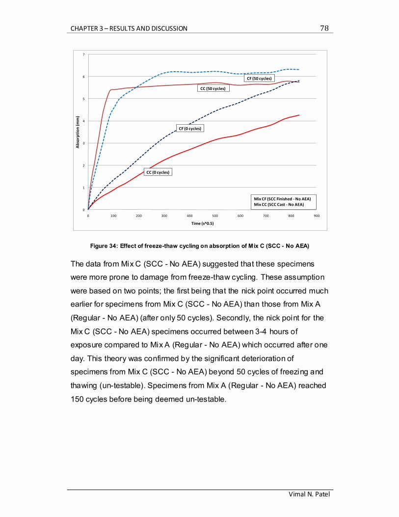
CHAPTER 3 – RESULTS AND DISCUSSION 78
Vimal N. Patel
Figure 34: Effect of freeze-thaw cycling on absorption of Mix C (SCC - No AEA)
The data from Mix C (SCC - No AEA) suggested that these specimens
were more prone to damage from freeze-thaw cycling. These assumption
were based on two points; the first being that the nick point occurred much
earlier for specimens from Mix C (SCC - No AEA) than those from Mix A
(Regular - No AEA) (after only 50 cycles). Secondly, the nick point for the
Mix C (SCC - No AEA) specimens occurred between 3-4 hours of
exposure compared to Mix A (Regular - No AEA) which occurred after one
day. This theory was confirmed by the significant deterioration of
specimens from Mix C (SCC - No AEA) beyond 50 cycles of freezing and
thawing (un-testable). Specimens from Mix A (Regular - No AEA) reached
150 cycles before being deemed un-testable.
0
1
2
3
4
5
6
7
0 100 200 300 400 500 600 700 800 900
Ab
sorp
tio
n (m
m)
Time (s^0.5)
CF (50 cycles)
CC (0 cycles)
CF (0 cycles)
CC (50 cycles)
Mix CF (SCC Finished - No AEA)Mix CC (SCC Cast - No AEA)
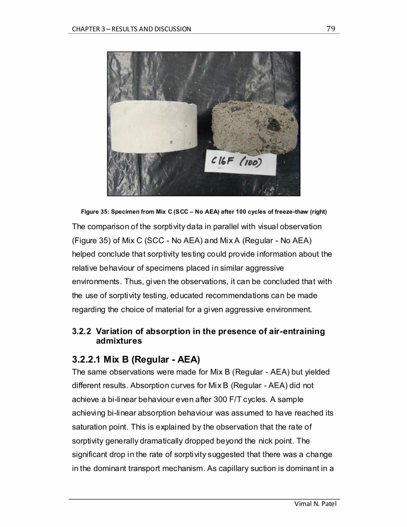
CHAPTER 3 – RESULTS AND DISCUSSION 79
Vimal N. Patel
Figure 35: Specimen from Mix C (SCC – No AEA) after 100 cycles of freeze-thaw (right)
The comparison of the sorptivity data in parallel with visual observation
(Figure 35) of Mix C (SCC - No AEA) and Mix A (Regular - No AEA)
helped conclude that sorptivity testing could provide information about the
relative behaviour of specimens placed in similar aggressive
environments. Thus, given the observations, it can be concluded that with
the use of sorptivity testing, educated recommendations can be made
regarding the choice of material for a given aggressive environment.
3.2.2 Variation of absorption in the presence of air-entraining admixtures
3.2.2.1 Mix B (Regular - AEA)
The same observations were made for Mix B (Regular - AEA) but yielded
different results. Absorption curves for Mix B (Regular - AEA) did not
achieve a bi-linear behaviour even after 300 F/T cycles. A sample
achieving bi-linear absorption behaviour was assumed to have reached its
saturation point. This is explained by the observation that the rate of
sorptivity generally dramatically dropped beyond the nick point. The
significant drop in the rate of sorptivity suggested that there was a change
in the dominant transport mechanism. As capillary suction is dominant in a
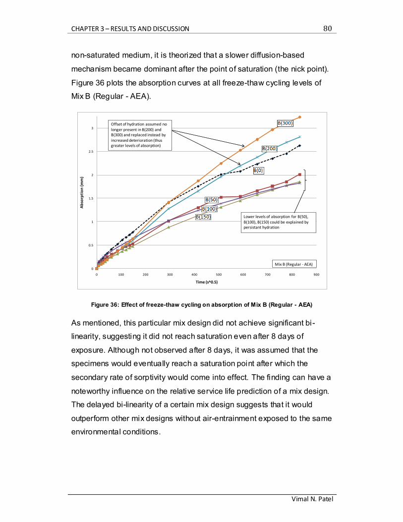
CHAPTER 3 – RESULTS AND DISCUSSION 80
Vimal N. Patel
non-saturated medium, it is theorized that a slower diffusion-based
mechanism became dominant after the point of saturation (the nick point).
Figure 36 plots the absorption curves at all freeze-thaw cycling levels of
Mix B (Regular - AEA).
Figure 36: Effect of freeze-thaw cycling on absorption of Mix B (Regular - AEA)
As mentioned, this particular mix design did not achieve significant bi-
linearity, suggesting it did not reach saturation even after 8 days of
exposure. Although not observed after 8 days, it was assumed that the
specimens would eventually reach a saturation point after which the
secondary rate of sorptivity would come into effect. The finding can have a
noteworthy influence on the relative service life prediction of a mix design.
The delayed bi-linearity of a certain mix design suggests that it would
outperform other mix designs without air-entrainment exposed to the same
environmental conditions.
0
0.5
1
1.5
2
2.5
3
0 100 200 300 400 500 600 700 800 900
Ab
sorp
tio
n (m
m)
Time (s^0.5)
Lower levels of absorption for B(50),B(100), B(150) could be explained by persistant hydration
Offset of hydration assumed no
longer present in B(200) and B(300) and replaced instead by increased deterioration (thus greater levels of absorption)
Mix B (Regular - AEA)
CHAPTER 3 – RESULTS AND DISCUSSION 81
Vimal N. Patel
3.2.2.2 Effect of hydration on the absorption behaviour
From Figure 36, it was seen that the samples subjected to 50, 100, and
150 freeze-thaw cycles outperformed the specimens subjected to zero
freeze-thaw cycles. This phenomenon was assumed to be caused by the
offset of continued hydration in specimens of Mix B (Regular - AEA). This
was not to say that specimens from other mixes did not have continued
hydration. Instead, it was considered that the damage incurred by freeze-
thaw cycling for specimens of other mixes was great enough to overcome
the offset of continued hydration. It was assumed that for specimens of
Mix B (Regular - AEA), the resistance to freeze-thaw cycling deterioration
from air-entrainment allowed water absorption to be allotted for hydration
purposes. The water absorption was the cause of increased hydration (i.e.
better quality concrete) instead of being the consequence of increased
deterioration.
3.2.3 Early-age and late-age sorptivity indicators
Figure 32 and Figure 33, show the early-age and late-age rate of
absorption values of all mixes for given exposure levels of freeze -thaw
cycling. From Figure 32, there exists a sharp increase in the sorptivity of
Mix A (Regular - No AEA), Mix CC (SCC Cast – No AEA), and Mix CF
(SCC Finished – No AEA) followed by a significant drop during the late-
age period. However, for Mix B (Regular - AEA) there was a steady
increase in the sorptivity rate throughout the early and late age. Upon
initial review, it may be suggested that Mix B (Regular - AEA)
demonstrated poorer performance relative to the other mix designs. This
was not the case, however, as visual inspection showed otherwise. It
should rather be considered that Mixes A (Regular - No AEA) and C (SCC
- No AEA) reached saturation during the early-age period, which was
followed by very low sorptivity rates during the late-age period.
Based on the results and the lack of absorption data of specimens
between 0 and 50 cycles of freeze-thaw cycling suggests that the step

CHAPTER 3 – RESULTS AND DISCUSSION 82
Vimal N. Patel
size of the sorptivity test should have been smaller. As with any other test,
a smaller step size would provide more detailed results. Unfortunately,
changes in step-sizes for sorptivity testing are often more demanding than
other tests. Thus, it should be recommended to carefully choose the
intervals of freeze-thaw cycling before testing to get an accurate estimate
of the shape of the absorption curves.
Based on the previously mentioned data, it can be said that the number of
freeze-thaw cycles can greatly affect the rate of absorption of a concrete
mix with no air-entraining admixture. It was suggested that the
identification of the nick point should be done carefully to not confuse low
overall rates of absorption with high initial rates absorption. The presence
of initial absorption, secondary absorption, and the nick point features in
the data reinforces the assumption that sorptivity testing can be used as a
viable testing method to provide information regarding service life
prediction.
3.3 Freeze-thaw resistance of self-compacting concrete
When assessing the freeze-thaw resistance of self-compacting concrete
through the absorption properties obtained from sorptivity testing, it can be
seen that self-consolidating concrete displays the poorest resistance to
deterioration. Conclusions where drawn based on results found from
absorption curves as can be seen in Figure 37 and Figure 38.
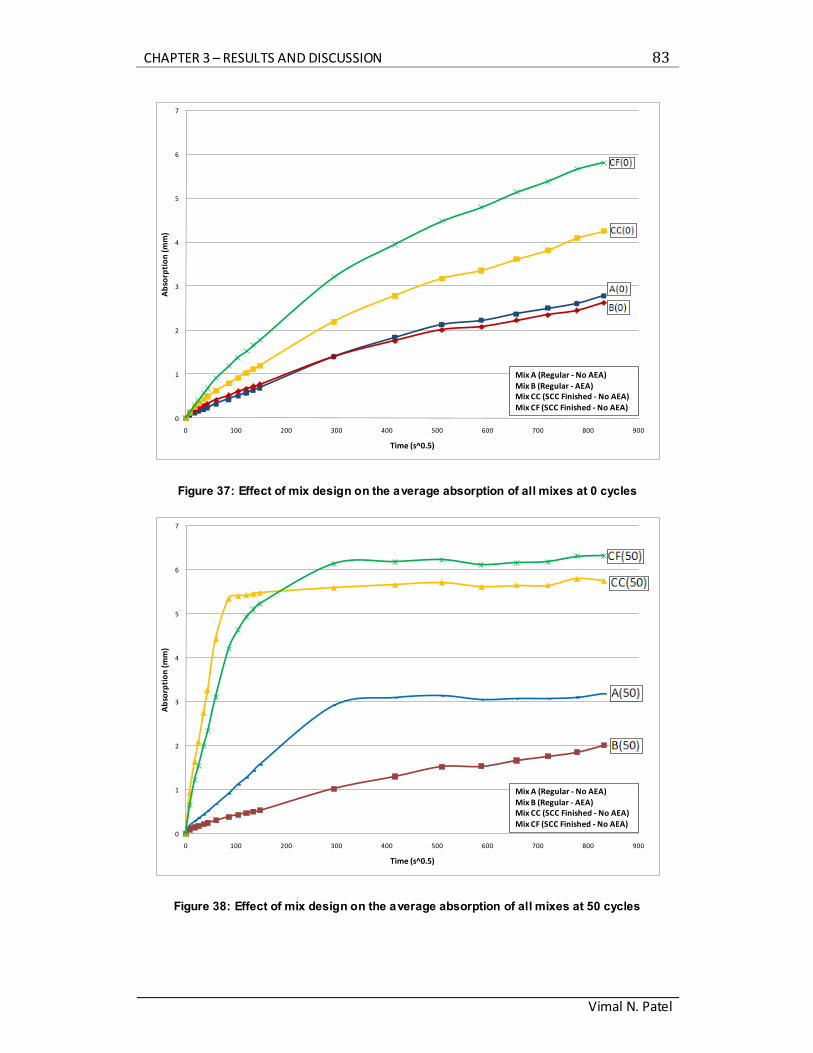
CHAPTER 3 – RESULTS AND DISCUSSION 83
Vimal N. Patel
Figure 37: Effect of mix design on the average absorption of all mixes at 0 cycles
Figure 38: Effect of mix design on the average absorption of all mixes at 50 cycles
0
1
2
3
4
5
6
7
0 100 200 300 400 500 600 700 800 900
Ab
sorp
tio
n (m
m)
Time (s^0.5)
Mix A (Regular - No AEA)Mix B (Regular - AEA) Mix CC (SCC Finished - No AEA) Mix CF (SCC Finished - No AEA)
0
1
2
3
4
5
6
7
0 100 200 300 400 500 600 700 800 900
Ab
sorp
tio
n (m
m)
Time (s^0.5)
Mix A (Regular - No AEA)Mix B (Regular - AEA) Mix CC (SCC Finished - No AEA) Mix CF (SCC Finished - No AEA)
CHAPTER 3 – RESULTS AND DISCUSSION 84
Vimal N. Patel
Even before the initiation of freeze-thaw cycling, the absorption of the SCC
mix was greater when compared to Mix A (Regular - No AEA) or Mix B
(Regular - AEA). Following exposure to 50 freeze-thaw cycles, the SCC
remained the mix with the greatest absorption. The steepness of the early-
age absorption suggests that the SCC mix was the fastest to reach
saturation. The location of the nick point showed that the SCC mix was the
first to reach saturation as well as having the greatest saturation capacity.
The high level of saturation suggests that the SCC mix was subjected to
severe deterioration and mass loss compared to Mix A (Regular - No AEA)
and Mix B (Regular - AEA). This led to the conclusion that the specimens
were more porous and permeable, which would translate into a material
that is highly susceptible to the ingress of deleterious materials. Analysis
of the density test results showed that the SCC had a greater volume of
permeable pore space (20.9%) compared to Mixes A (Regular - No AEA)
(16.1%) and B (Regular - AEA) (15.1%). The lack of air entrainment in Mix
C (SCC - No AEA) translated into a system that was not comprised of
small air voids with a small spacing factor but instead a high porosity mix
with larges voids spaced further apart. This suggests that the results from
the density test could have been used as preliminary indicators of the
relative performance of each mix design.
The strength of the SCC mix (26.12 MPa) was 88% that of Mix B (Regular
- AEA) (29.73 MPa). But the absorption of Mix C (SCC - No AEA) was
168% greater than Mix B (Regular - AEA). This disparity suggests that
strength cannot be used as the paramount criterion in determining the
durability performance of a concrete specimen. This in addition to the
severe deterioration of specimens exposed to more than 50 freeze-thaw
cycles suggests that the mix design of the SCC has an important
implication as to the durability of the specimens. The deterioration of the
specimens subjected to 100, 150 and 200 cycles can be seen in Figure
39. All specimens exposed to more than 50 freeze-thaw cycles were
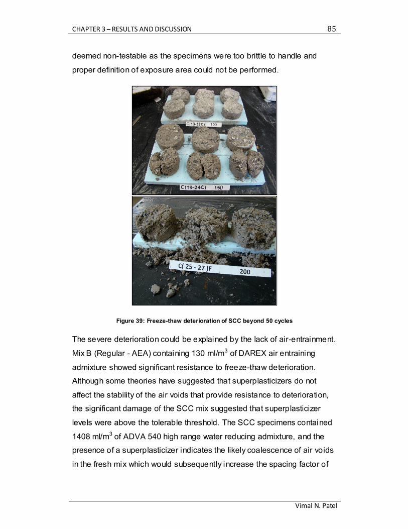
CHAPTER 3 – RESULTS AND DISCUSSION 85
Vimal N. Patel
deemed non-testable as the specimens were too brittle to handle and
proper definition of exposure area could not be performed.
Figure 39: Freeze-thaw deterioration of SCC beyond 50 cycles
The severe deterioration could be explained by the lack of air-entrainment.
Mix B (Regular - AEA) containing 130 ml/m3 of DAREX air entraining
admixture showed significant resistance to freeze-thaw deterioration.
Although some theories have suggested that superplasticizers do not
affect the stability of the air voids that provide resistance to deterioration,
the significant damage of the SCC mix suggested that superplasticizer
levels were above the tolerable threshold. The SCC specimens contained
1408 ml/m3 of ADVA 540 high range water reducing admixture, and the
presence of a superplasticizer indicates the likely coalescence of air voids
in the fresh mix which would subsequently increase the spacing factor of
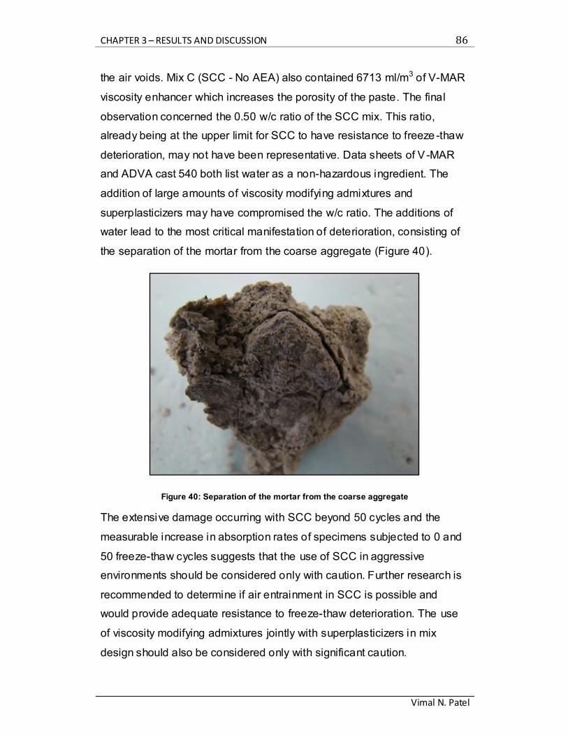
CHAPTER 3 – RESULTS AND DISCUSSION 86
Vimal N. Patel
the air voids. Mix C (SCC - No AEA) also contained 6713 ml/m3 of V-MAR
viscosity enhancer which increases the porosity of the paste. The final
observation concerned the 0.50 w/c ratio of the SCC mix. This ratio,
already being at the upper limit for SCC to have resistance to freeze -thaw
deterioration, may not have been representative. Data sheets of V -MAR
and ADVA cast 540 both list water as a non-hazardous ingredient. The
addition of large amounts of viscosity modifying admixtures and
superplasticizers may have compromised the w/c ratio. The additions of
water lead to the most critical manifestation of deterioration, consisting of
the separation of the mortar from the coarse aggregate (Figure 40).
Figure 40: Separation of the mortar from the coarse aggregate
The extensive damage occurring with SCC beyond 50 cycles and the
measurable increase in absorption rates of specimens subjected to 0 and
50 freeze-thaw cycles suggests that the use of SCC in aggressive
environments should be considered only with caution. Further research is
recommended to determine if air entrainment in SCC is possible and
would provide adequate resistance to freeze-thaw deterioration. The use
of viscosity modifying admixtures jointly with superplasticizers in mix
design should also be considered only with significant caution.
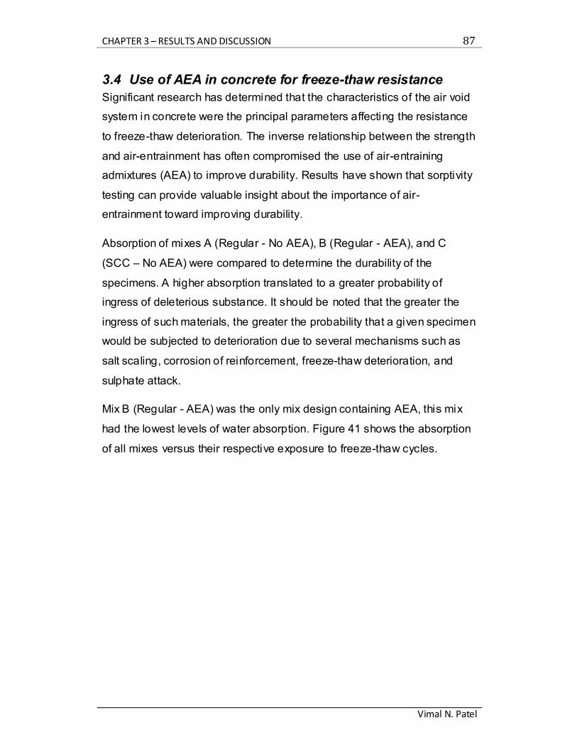
CHAPTER 3 – RESULTS AND DISCUSSION 87
Vimal N. Patel
3.4 Use of AEA in concrete for freeze-thaw resistance
Significant research has determined that the characteristics of the air void
system in concrete were the principal parameters affecting the resistance
to freeze-thaw deterioration. The inverse relationship between the strength
and air-entrainment has often compromised the use of air-entraining
admixtures (AEA) to improve durability. Results have shown that sorptivity
testing can provide valuable insight about the importance of air-
entrainment toward improving durability.
Absorption of mixes A (Regular - No AEA), B (Regular - AEA), and C
(SCC – No AEA) were compared to determine the durability of the
specimens. A higher absorption translated to a greater probability of
ingress of deleterious substance. It should be noted that the greater the
ingress of such materials, the greater the probability that a given specimen
would be subjected to deterioration due to several mechanisms such as
salt scaling, corrosion of reinforcement, freeze-thaw deterioration, and
sulphate attack.
Mix B (Regular - AEA) was the only mix design containing AEA, this mix
had the lowest levels of water absorption. Figure 41 shows the absorption
of all mixes versus their respective exposure to freeze-thaw cycles.
CHAPTER 3 – RESULTS AND DISCUSSION 88
Vimal N. Patel
Figure 41: Effect of mix design on the total absorption at given levels of freeze-thaw cycling
From Figure 41, it was clear that Mix B (Regular - AEA) significantly
outperformed all other mixes in terms of total absorption over al l levels of
freeze-thaw cycles. The total absorption (i.e. increase in susceptibility to
deterioration) only began to increase after 200 freeze-thaw cycles, before
which no significant damage could be detected. Additionally, only Mix B
(Regular - AEA) was testable up to 300 cycles. Figure 42 shows the state
of the specimens following 200 freeze-thaw cycles.
0.00
1.00
2.00
3.00
4.00
5.00
6.00
7.00
0 50 100 150 200 250 300
Tota
l Ab
sorp
tio
n o
ver
8 d
ays
(mm
)
Freeze Thaw Cycles
Mix CF (SCC Finished - No AEA)
Mix CC (SCC Cast - No AEA)
Mix A (Regular - No AEA)
Mix B (Regular - AEA)
Specimens no longer testable due to severe damage
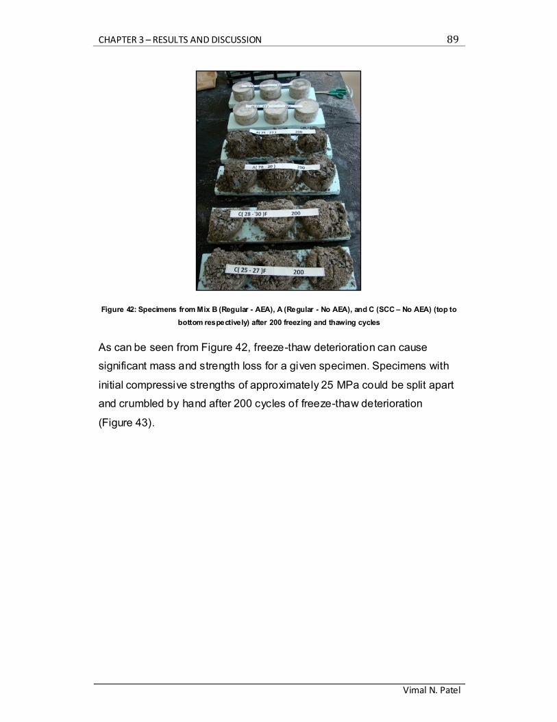
CHAPTER 3 – RESULTS AND DISCUSSION 89
Vimal N. Patel
Figure 42: Specimens from Mix B (Regular - AEA), A (Regular - No AEA), and C (SCC – No AEA) (top to
bottom respectively) after 200 freezing and thawing cycles
As can be seen from Figure 42, freeze-thaw deterioration can cause
significant mass and strength loss for a given specimen. Specimens with
initial compressive strengths of approximately 25 MPa could be split apart
and crumbled by hand after 200 cycles of freeze-thaw deterioration
(Figure 43).
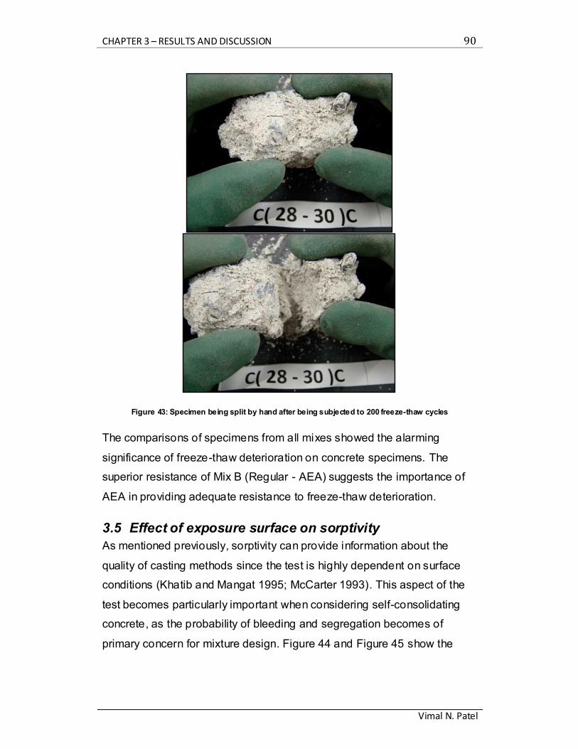
CHAPTER 3 – RESULTS AND DISCUSSION 90
Vimal N. Patel
Figure 43: Specimen being split by hand after being subjected to 200 freeze-thaw cycles
The comparisons of specimens from all mixes showed the alarming
significance of freeze-thaw deterioration on concrete specimens. The
superior resistance of Mix B (Regular - AEA) suggests the importance of
AEA in providing adequate resistance to freeze-thaw deterioration.
3.5 Effect of exposure surface on sorptivity
As mentioned previously, sorptivity can provide information about the
quality of casting methods since the test is highly dependent on surface
conditions (Khatib and Mangat 1995; McCarter 1993). This aspect of the
test becomes particularly important when considering self-consolidating
concrete, as the probability of bleeding and segregation becomes of
primary concern for mixture design. Figure 44 and Figure 45 show the
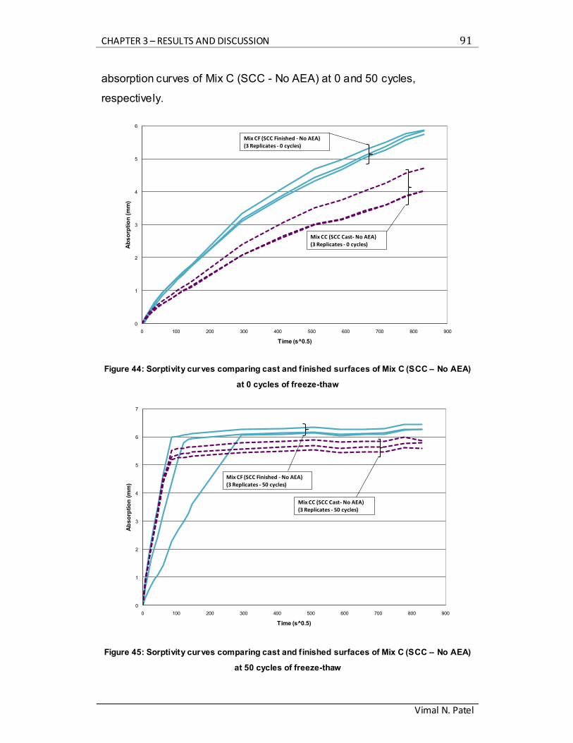
CHAPTER 3 – RESULTS AND DISCUSSION 91
Vimal N. Patel
absorption curves of Mix C (SCC - No AEA) at 0 and 50 cycles,
respectively.
Figure 44: Sorptivity curves comparing cast and finished surfaces of Mix C (SCC – No AEA)
at 0 cycles of freeze-thaw
Figure 45: Sorptivity curves comparing cast and finished surfaces of Mix C (SCC – No AEA)
at 50 cycles of freeze-thaw
0
1
2
3
4
5
6
0 100 200 300 400 500 600 700 800 900
Ab
so
rpti
on
(m
m)
Time (s^0.5)
Mix CF (SCC Finished - No AEA)(3 Replicates - 0 cycles)
Mix CC (SCC Cast- No AEA)(3 Replicates - 0 cycles)
0
1
2
3
4
5
6
7
0 100 200 300 400 500 600 700 800 900
Ab
so
rpti
on
(m
m)
Time (s^0.5)
Mix CC (SCC Cast- No AEA)(3 Replicates - 50 cycles)
Mix CF (SCC Finished - No AEA)(3 Replicates - 50 cycles)
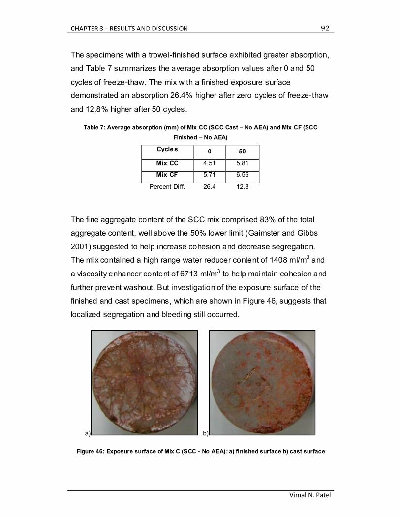
CHAPTER 3 – RESULTS AND DISCUSSION 92
Vimal N. Patel
The specimens with a trowel-finished surface exhibited greater absorption,
and Table 7 summarizes the average absorption values after 0 and 50
cycles of freeze-thaw. The mix with a finished exposure surface
demonstrated an absorption 26.4% higher after zero cycles of freeze-thaw
and 12.8% higher after 50 cycles.
Table 7: Average absorption (mm) of Mix CC (SCC Cast – No AEA) and Mix CF (SCC
Finished – No AEA)
Cycles 0 50
Mix CC 4.51 5.81
Mix CF 5.71 6.56
Percent Diff. 26.4 12.8
The fine aggregate content of the SCC mix comprised 83% of the total
aggregate content, well above the 50% lower limit (Gaimster and Gibbs
2001) suggested to help increase cohesion and decrease segregation.
The mix contained a high range water reducer content of 1408 ml/m3 and
a viscosity enhancer content of 6713 ml/m3 to help maintain cohesion and
further prevent washout. But investigation of the exposure surface of the
finished and cast specimens, which are shown in Figure 46, suggests that
localized segregation and bleeding sti ll occurred.
a) b)
Figure 46: Exposure surface of Mix C (SCC - No AEA): a) finished surface b) cast surface
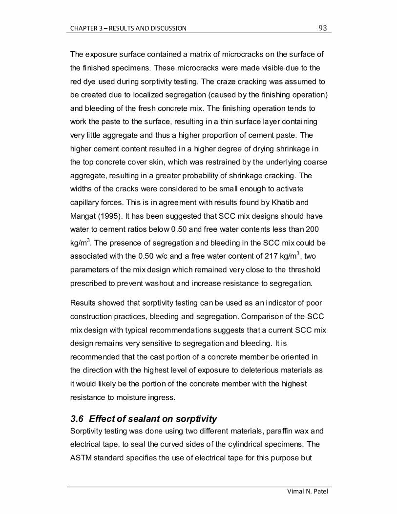
CHAPTER 3 – RESULTS AND DISCUSSION 93
Vimal N. Patel
The exposure surface contained a matrix of microcracks on the surface of
the finished specimens. These microcracks were made visible due to the
red dye used during sorptivity testing. The craze cracking was assumed to
be created due to localized segregation (caused by the finishing operation)
and bleeding of the fresh concrete mix. The finishing operation tends to
work the paste to the surface, resulting in a thin surface layer containing
very little aggregate and thus a higher proportion of cement paste. The
higher cement content resulted in a higher degree of drying shrinkage in
the top concrete cover skin, which was restrained by the underlying coarse
aggregate, resulting in a greater probability of shrinkage cracking. The
widths of the cracks were considered to be small enough to activate
capillary forces. This is in agreement with results found by Khatib and
Mangat (1995). It has been suggested that SCC mix designs should have
water to cement ratios below 0.50 and free water contents less than 200
kg/m3. The presence of segregation and bleeding in the SCC mix could be
associated with the 0.50 w/c and a free water content of 217 kg/m3, two
parameters of the mix design which remained very close to the threshold
prescribed to prevent washout and increase resistance to segregation.
Results showed that sorptivity testing can be used as an indicator of poor
construction practices, bleeding and segregation. Comparison of the SCC
mix design with typical recommendations suggests that a current SCC mix
design remains very sensitive to segregation and bleeding. It is
recommended that the cast portion of a concrete member be oriented in
the direction with the highest level of exposure to deleterious materials as
it would likely be the portion of the concrete member with the highest
resistance to moisture ingress.
3.6 Effect of sealant on sorptivity
Sorptivity testing was done using two different materials, paraffin wax and
electrical tape, to seal the curved sides of the cylindrical specimens. The
ASTM standard specifies the use of electrical tape for this purpose but

CHAPTER 3 – RESULTS AND DISCUSSION 94
Vimal N. Patel
doubts arose as to its effectiveness since it was observed that water was
being drawn up between the tape and the concrete surface. Thus, an
investigation was conducted to evaluate whether paraffin wax would
perform better.
Upon visual review of the sorptivity curves (Figure 46), the specimens
sealed using electrical tape displayed greater absorption than those
coated with paraffin wax. As well, the specimens sealed with electrical
tape exhibited greater variability than those sealed with wax. The results
confirmed theories which stated that the boundary conditions used in
sorptivity testing greatly affect the absorption results (Caliskan 2006;
Claisse 1997; Gonen and Yazicioglu 2007; Martys and Ferraris 1997;
Taha 2001).
Figure 47: Absorption curves comparing waxed and taped specimens of Mix B (Regular –
AEA) at 150 cycles of freeze-thaw
It was assumed that the additional absorption present in specimens sealed
with electrical tape could be explained by the poor seal along the edges of
the exposure surface. The poor adherence of the electrical tape would
0
0.5
1
1.5
2
2.5
3
0 100 200 300 400 500 600 700 800 900
Ab
sorp
tio
n (m
m)
Time (s^0.5)
Mix B Waxed (Regular - AEA)(3 Replicates - 150 cycles)
Mix B Taped (Regular - AEA)(3 Replicates - 150 cycles)
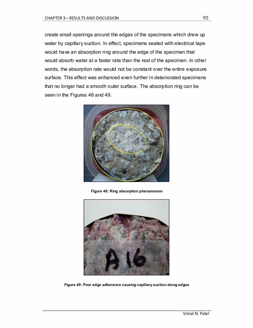
CHAPTER 3 – RESULTS AND DISCUSSION 95
Vimal N. Patel
create small openings around the edges of the specimens which drew up
water by capillary suction. In effect, specimens sealed with electrical tape
would have an absorption ring around the edge of the specimen that
would absorb water at a faster rate than the rest of the specimen. In other
words, the absorption rate would not be constant over the entire exposure
surface. This effect was enhanced even further in deteriorated specimens
that no longer had a smooth outer surface. The absorption ring can be
seen in the Figures 48 and 49.
Figure 48: Ring absorption phenomenon
Figure 49: Poor edge adherence causing capillary suction along edges
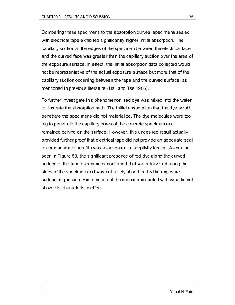
CHAPTER 3 – RESULTS AND DISCUSSION 96
Vimal N. Patel
Comparing these specimens to the absorption curves, specimens sealed
with electrical tape exhibited significantly higher initial absorption. The
capillary suction at the edges of the specimen between the electrical tape
and the curved face was greater than the capillary suction over the area of
the exposure surface. In effect, the initial absorption data collected would
not be representative of the actual exposure surface but more that of the
capillary suction occurring between the tape and the curved surface, as
mentioned in previous literature (Hall and Tse 1986).
To further investigate this phenomenon, red dye was mixed into the water
to illustrate the absorption path. The initial assumption that the dye would
penetrate the specimens did not materialize. The dye molecules were too
big to penetrate the capillary pores of the concrete specimen and
remained behind on the surface. However, this undesired result actually
provided further proof that electrical tape did not provide an adequate seal
in comparison to paraffin wax as a sealant in sorptivity testing. As can be
seen in Figure 50, the significant presence of red dye along the curved
surface of the taped specimens confirmed that water travelled along the
sides of the specimen and was not solely absorbed by the exposure
surface in question. Examination of the specimens sealed with wax did not
show this characteristic effect.
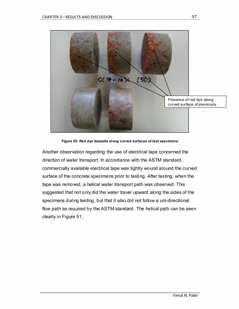
CHAPTER 3 – RESULTS AND DISCUSSION 97
Vimal N. Patel
Figure 50: Red dye deposits along curved surfaces of test specimens
Another observation regarding the use of electrical tape concerned the
direction of water transport. In accordance with the ASTM standard,
commercially available electrical tape was tightly wound around the curved
surface of the concrete specimens prior to testing. After testing, when the
tape was removed, a helical water transport path was observed. This
suggested that not only did the water travel upward along the sides of the
specimens during testing, but that it also did not follow a uni-directional
flow path as required by the ASTM standard. The helical path can be seen
clearly in Figure 51.
Presence of red dye along
curved surface of previously taped specimens

CHAPTER 3 – RESULTS AND DISCUSSION 98
Vimal N. Patel
Figure 51: Helical transport path of water
Statistical analysis on the rates of early-age (0-6 hours) and late-age (1-8
days) absorption further reinforced visual inspection. The F-test was used
to examine variability (with an 80% confidence interval) and the student-T
test was used to evaluate the significance of differences in sample means.
Table 8 consists of contingency tables that summarize the number of
times either the variance or mean of specimens tested with electrical tape
or wax was greater, and as well as the number of times the statistical
analysis resulted in a null hypothesis (no significant difference between
the variance or mean of samples tested with electrical tape or wax.).
Table 8: Summary of results of statistical analysis
As can be seen from Table 8, the variance within specimens tested with
electrical tape was found to be significantly greater 7 times out of 14
during early-age absorption measurements and 8 times out of 14 during
Tape Greater Wax Greater Null Total Tape Greater Wax Greater Null Total
A 2 0 2 4 A 3 1 0 4
B 3 0 3 6 B 4 0 2 6
CC 1 0 1 2 CC 2 0 0 2
CF 1 1 0 2 CF 0 0 2 2
Total 7 1 6 14 Total 9 1 4 14
Tape Greater Wax Greater Null Total Tape Greater Wax Greater Null Total
A 3 0 1 4 A 2 0 2 4
B 5 0 1 6 B 1 1 4 6
CC 0 0 2 2 CC 1 0 1 2
CF 0 0 2 2 CF 1 0 1 2
Total 8 0 6 14 Total 5 1 8 14
T-Test Summary for Means
(1-8 Days) 80% Confidence
F-Test Summary for Variances
(0-6 Hours) 80% Confidence
T-Test Summary for Means
(0-6 Hours) 80% Confidence
F-Test Summary for Variances
(1-8 Days) 80% Confidence
CHAPTER 3 – RESULTS AND DISCUSSION 99
Vimal N. Patel
late-age absorption. The mean of specimens tested with e lectrical tape
was significantly greater 9 times out of 14 during early-age absorption and
5 times out of 14 during late-age absorption with 8 null results. The results
of the statistical analysis are further detailed in the appendix.
In conclusion, the uniformity of the wax sealed specimens was greater
than the specimens sealed with electrical tape, as the latter specimens
were susceptible to greater absorption and variable transportation
properties. After having visually inspected the specimens and analysed
the data, it can be concluded that paraffin wax is a superior sealant for
sorptivity testing in comparison to electrical tape.

CONCLUSIONS 100
Vimal N. Patel
CONCLUSIONS
Three mixes: Mix A (Regular - No AEA), Mix B (Regular - AEA), and Mix C
(SCC - No AEA) were subjected to various levels of freeze-thaw cycling
and were tested for absorption. All mixes were subjected to the same
curing, conditioning, and exposure environment leaving only the mix
design parameters to influence the sorptivity behaviour of the specimens.
The absorption behaviour of Mix A (Regular - No AEA) showed an acute
bi-linearity after one day of exposure. Mix C (SCC - No AEA)
demonstrated this same behaviour after only 4 hours of exposure. The
SCC mix design absorbed more water at a faster rate suggesting that
SCC mix designs could be highly susceptible to the ingress of deleterious
materials and deterioration from freeze-thaw cycling. Comparison of Mix A
(Regular - No AEA) and Mix B (Regular - AEA), showed that Mix B
(Regular - AEA) did not demonstrate significant bi-linearity in the
absorption behaviour even after 8 days suggesting increased durability.
Furthermore, the presence of air-entrainment in Mix B (Regular - AEA)
allowed for continued hydration to offset the absorption by forming a
denser matrix during freeze-thaw cycling. Consequently, Mix B (Regular -
AEA) had the lowest level of total absorption.
The high early-age absorption of Mix A (Regular - No AEA) and Mix C
(SCC - No AEA), followed by a significant drop during the late-age
absorption, suggested that the step size of sorptivity testing should be
carefully selected as intervals between 0 and 50 cycles could show
significant variability and provide valuable data concerning the absorption
behaviour.
Sorptivity testing was considered sensitive enough to differentiate between
exposure surfaces of the SCC mix. It was shown that the finished surface
CONCLUSIONS 101
Vimal N. Patel
was more susceptible to absorption due to segregation and bleeding,
which led to craze cracking at the top surface.
Finally, the ASTM Standard C 1585-04 testing method was analyzed to
determine the adequacy of the material used to seal the curved surfaces.
Results showed that electrical tape produced increased absorption totals
as well as increased data variability. F and student-t test results concluded
that paraffin wax was a better choice of sealant for sorptivity testing.
REFERENCES 102
Vimal N. Patel
REFERENCES
Aïtcin, P. C. (2003). "The durability characteristics of high performance concrete: a review." Cement and Concrete Composites, 25(4-5),
409-420. Aldea, C., Shah, S., and Karr, A. (1999). "Permeability of cracked
concrete." Materials and Structures, 32(5), 370-376.
Assie, S., Escadeillas, G., and Waller, V. (2007). "Estimates of self-compacting concrete 'potential' durability." Construction and Building Materials, 21(10), 1909-1917.
Bai, J., Wild, S., and Sabir, B. B. (2002). "Sorptivity and strength of air-
cured and water-cured PC-PFA-MK concrete and the influence of binder composition on carbonation depth." Cement and Concrete Research, 32(11), 1813-1821.
Bartos, P., and Grauers, M. (1999). "Self-compacting concrete." Concrete,
9-13. Basheer, L., Kropp, J., and Cleland, D. (2001). "Assessment of the
durability of concrete from its permeation properties: a review." Construction and Building Materials, 15(2-3), 93-103.
Bentz, D., Ehlen, M., Ferraris, C., and Garboczi, E. "Sorptivity-Based
Service Life Predictions for Concrete Pavements." 181–193.
Bentz, D. P., Garboczi, E. J., Haecker, C. J., and Jensen, O. M. (1999).
"Effects of cement particle size distribution on performance properties of Portland cement-based materials." Cement and Concrete Research, 29(10), 1663-1671.
Bickley, J. A., and Mitchell, D. (2001). "A state-of-the-art review of high
performance concrete structures built in Canada: 1990-2000." Canada, 1-114.
Bruere, G. M. (1955). "Air entrainment in cement and silica pastes." ACI Journal Proceedings, 51(5), 905-919.
Caliskan, S. (2006). "Influence of curing conditions on the sorptivity and
weight change characteristics of self-compacting concrete." The
Arabian Journal for Science and Engineering, 31(1), 169-178.

REFERENCES 103
Vimal N. Patel
Chatterji, S. (2003). "Freezing of air-entrained cement-based materials
and specific actions of air-entraining agents." Cement and Concrete Composites, 25(7), 759-765.
Claisse, P. A. (1997). "Absorption and Sorptivity of Cover Concrete."
Journal of Materials in Civil Engineering, 9(3), 105-110.
Cohen, M. D. (1992). "Non-Air-Entrained High-Strength Concrete--Is it
Frost Resistant?" ACI Materials Journal, 89(4). Collins, M. P. (1993). "Structural Design Considerations for High Strength
Concrete." Concrete International, 15, 27.
Damgaard Jensen, A., and Chatterji, S. (1996). "State of the art report on micro-cracking and lifetime of concrete—Part 1." Materials and Structures, 29(1), 3-8.
DeSouza, S. J., Hooton, R. D., and Bickley, J. A. (1997). "Evaluation of
laboratory drying procedures relevant to field conditions for concrete sorptivity measurements." Cement, concrete and aggregates, 19(2), 59-63.
Desouza, S. J., Hooton, R. D., and Bickley, J. A. (1998). "A field test for
evaluating high performance concrete covercrete quality." Canadian Journal of Civil Engineering, 25(3), 551-556.
Dhir, R. K., and Hewlett, P. C. (1987). "Near surface characteristics of concrete: assessment and development of in-situ test methods."
Magazine of Concrete Research, London U.K, 183-195. Dias, W. P. S. (2000). "Reduction of concrete sorptivity with age through
carbonation." Cement and Concrete Research, 30(8), 1255-1261.
Dias, W. P. S. (2004). "Influence of drying on concrete sorptivity." Magazine of Concrete Research.
Du, L., and Folliard, K. J. (2005). "Mechanisms of air entrainment in concrete." Cement and Concrete Research, 35(8), 1463-1471.
Ekenel, M., and Myers, J. J. (2005). "Durability performance of bridge
concretes, Part 2: High-strength concrete (HSC)." Journal of ASTM
International, 2(7), 1-11.
El-Dieb, A. (2007). "Self-curing concrete: Water retention, hydration and moisture transport." Construction and Building Materials, 21(6), 1282-1287.
REFERENCES 104
Vimal N. Patel
Fagerlund, G. (1971). "Degré critique de saturation un outil pour
l'estimation de la résistance au gel des matériaux de construction." Materials and Structures, 4(5), 271-285.
Ferraris, C., and Stutzman, P. (2006). "Sulfate Resistance of Concrete: a
New Approach and Test." PCA R&D Serial, 2486, 1-78.
Gaimster, R. (2000). "Self-compacting concrete " Concrete, 34(4), 23-25.
Gaimster, R., and Gibbs, J. (2001). "Self-compacting concrete. Part 1: The
material and its properties." Concrete, 35(7), 32-34.
Gonen, T., and Yazicioglu, S. (2007). "The influence of compaction pores
on sorptivity and carbonation of concrete." Construction and Building Materials, 21(5), 1040-1045.
Hall, C. (1977). "Water movement in porous building materials--I. Unsaturated flow theory and its applications." Building and
Environment, 12(2), 117-125. Hall, C. (1981). "Water movement in porous building materials--IV. The
initial surface absorption and the sorptivity." Building and Environment, 16(3), 201-207.
Hall, C., and Raymond Yau, M. H. (1987). "Water movement in porous
building materials--IX. The water absorption and sorptivity of
concretes." Building and Environment, 22(1), 77-82.
Hall, C., and Tse, T. K.-M. (1986). "Water movement in porous building materials--VII. The sorptivity of mortars." Building and Environment, 21(2), 113-118.
Henderson, N. (2000). "Self-compacting concrete at Millennium Point."
Concrete, 34(4), 26-27. Ho, D. W. S., and Chirgwin, G. J. (1996). "A performance specification for
durable concrete." Construction and Building Materials, 10(5), 375-379.
Ho, D. W. S., Cui, Q. Y., and Ritchie, D. J. (1989). "The influence of
humidity and curing time on the quality of concrete." Cement and
Concrete Research, 19(3), 457-464.
Ho, D. W. S., and Lewis, R. K. (1988). "The specification of concrete for reinforcement protection-- performance criteria and compliance by strength." Cement and Concrete Research, 18(4), 584-594.
REFERENCES 105
Vimal N. Patel
Jacobsen, S., Sellevold, E. J., and Matala, S. (1996). "Frost durability of
high strength concrete: Effect of internal cracking on ice formation." Cement and Concrete Research, 26(6), 919-931.
Khatib, J. M., and Mangat, P. S. (1995). "Absorption characteristics of
concrete as a function of location relative to casting position."
Cement and Concrete Research, 25(5), 999-1010.
Khayat, K., and Assaad, J. (2002). "Air-void stability in self-consolidating concrete " ACI Materials Journal, 99(4), 408-416.
Khayat, K. H. (1995). "Frost durability of concrete containing viscosity-modifying admixtures." ACI Materials Journal, 92(6), 625-633.
Khayat, K. H. (2000). "Optimization and performance of air-entrained, self-
consolidating concrete." ACI Materials Journal, 97(5), 526-535.
Krauss, P., and Rogalla, E. (1996). Transverse Cracking in Newly
Constructed Bridge Decks, Transportation Research Board. Lachemi, M., Hossain, K. M. A., Lambros, V., Nkinamubanzi, P. C., and
Bouzouba‚, N. (2004a). "Performance of new viscosity modifying admixtures in enhancing the rheological properties of cement
paste." Cement and Concrete Research, 34(2), 185-193. Lachemi, M., Hossain, K. M. A., Lambros, V., Nkinamubanzi, P. C., and
Bouzouba‚, N. (2004b). "Self-consolidating concrete incorporating new viscosity modifying admixtures." Cement and Concrete
Research, 34(6), 917-926. Levitt, M. "Non-destructive testing of concrete by the initial surface
absorption method." Symposium on Non-Destructive Testing of Concrete and Timber, London U.K, 23-26.
Litvan, G. G. (1972). "Phase Transitions of Adsorbates: IV, Mechanism of
Frost Action in Hardened Cement Paste*." Journal of the American
Ceramic Society, 55(1), 38-42.
Litvan, G. G. (1973). "Frost action in cement paste." Materials and Structures, 6(4), 293-298.
Litvan, G. G. (1983). "Air entrainment in the presence of superplasticizers." Journal of American Concrete Institute , 80(4),
326-331.
REFERENCES 106
Vimal N. Patel
Martys, N. S., and Ferraris, C. F. (1997). "Capillary transport in mortars
and concrete." Cement and Concrete Research, 27(5), 747-760.
McCarter, W. J. (1993). "Influence of Surface Finish on Sorptivity on Concrete." Journal of Materials in Civil Engineering, 5(1), 130-136.
McDonald, D., Krauss, P., and Rogalla, E. (1995). "Early-Age Transverse Deck Cracking." Concrete International, 17(5), 49-51.
Mehta, P. K. (1997). "Durability-Critical Issues for the Future." Concrete
International, 19(7), 27.
Mehta, P. K. (1999). "Advancements in Concrete Technology." Concrete
International, 21, 69. Mehta, P. K., and Burrows, R. W. (2001). "Building durable structures in
the 21st century." The Indian Concrete Journal, 437-443.
Mielenz, R. C., Wolkodoff, V. E., Backstrom, J. E., and Flack, H. L. (1958a). "Origin, Evolution, and Effects of the Air Void System in Concrete. Part 1 - Entrained air in unhardend Concrete." Journal of
American Concrete Institute, 55(7), 95-121.
Mielenz, R. C., Wolkodoff, V. E., Backstrom, J. E., and Flack, H. L. (1958b). "Origin, Evolution, and Effects of the Air Void System in Concrete. Part 2 - Influence of type and amount of air-entraining
agent." Journal of American Concrete Institute, 55(8), 261-272.
Mielenz, R. C., Wolkodoff, V. E., Backstrom, J. E., and Flack, H. L. (1958c). "Origin, Evolution, and Effects of the Air Void System in Concrete. Part 3 - Influence of water-cement ratio and compaction."
Journal of American Concrete Institute , 55(8), 359-375.
Mindess, S., Darwin, D., and Young, F. J. (1981). Concrete, 2nd Ed., Prentice Hall, c2003, Upper Saddle River, NJ.
Nevi lle, A., and Aïtcin, P.-C. (1998). "High performance concrete—An overview." Materials and Structures, 31(2), 111-117.
Obla, K. (2006). "Experimental case study demonstrating advantages of
performance specifications." RMC Research Foundation, 1-19.
Okamura, H., and Ouchi, M. (2002). "Self-compacting concrete." Journal
of Advanced Concrete Technology, 1(1), 5-15.
REFERENCES 107
Vimal N. Patel
Persson, B. (2001). "A comparison between mechanical properties of self-
compacting concrete and the corresponding properties of normal concrete." Cement and Concrete Research, 31(2), 193-198.
Pigeon, M. (1989). "La durabilité au gel du béton." Materials and
Structures, 22(1), 3-14.
Pigeon, M. (1995). Durability of Concrete in Cold Climates.
Pigeon, M., and Lachance, M. (1981). "Critical air-void spacing factors for
concretes submitted to slow freeze-thaw cycles." Journal of
American Concrete Institute, 78(4), 282-291.
Pigeon, M., Pleau, R., and Aitchin, P. (1986). "Freeze-thaw durability of concrete with anc without silica fume in ASTM C 666(procedure A) test method: internal cracking versus scaling." Cement, concrete
and aggregates, 8(2), 76-85.
Pigeon, M., Prevost, J., and Simard, J. (1985). "Freeze-Thaw Durability versus Freezing Rate." Journal of the American Concrete Institute, 684-92.
Plante, P., Pigeon, M., and Saucier, F. (1989). "Air-void stability, Part II:
Influence of superplasticizers and cement." ACI Materials Journal, 86(6), 581-589.
Powers, T. C. (1945). "A working hypothesis for further studies of frost resistance." Journal of American Concrete Institute, 16(4), 245-272.
Powers, T. C. (1949). "The air requirement of frost resistant-concrete."
Proceedings of the Highway Research Board, 29, 184-211.
Powers, T. C. (1975). "Freezing effects in concrete." ACI Special
Publication SP-47, American Concrete Institute, Detroit, MI, 1-11. Powers, T. C. (2003). "Studies of the physical properties of hardened
portland cement paste." Concrete International, 25(8), 59.
Powers, T. C., and Helmuth, R. A. (1953). "Theory of volume changes in hardened Portland cement pastes during freezing." Proceedings of the Highway Research Board, 32, 285-297.
Radlinski, M., Olek, J., and Nantung, T. (2007). "Evaluation of Transport
Properties of Ternary (OPC/FA/SF) Concrete Mixtures Using Migration and Absorption-Type Tests." Special Publication, 242, 481-496.
REFERENCES 108
Vimal N. Patel
Rasheeduzzafar, F. H. D. (1990). "Influence of Cement Composition on
the Corrosion of Reinforcement and Sulfate Resistance of Concrete." ACI Materials Journal, 87(2).
Rols, S., Ambroise, J., and Pera, J. (1999). "Effects of different viscosity
agents on the properties of self-leveling concrete." Cement and
Concrete Research, 29(2), 261-266.
Rose, K., Hope, B. B., and Ip, A. K. C. (1989). "Statistical analysis of strength and durability of concrete made with different cements." Cement and Concrete Research, 19(3), 476-486.
Sabir, B. B. (1998). "A water sorptivity test for mortar and concrete."
Materials and Structures, 31(8), 568-574. Saucier, F., Pigeon, M., and Plante, P. (1990). "Air-void stability, Part III:
Field tests for superplasticized concretes." ACI Materials Journal, 87(1), 3-11.
Sun, W., Zhang, Y. M., Yan, H. D., and Mu, R. (1999). "Damage and
damage resistance of high strength concrete under the action of
load and freeze-thaw cycles." Cement and Concrete Research, 29(9), 1519-1523.
Taha, M. M. R. (2001). "Sorptivity: a reliable measurement for surface
absorption of masonry brick units." Materials and Structures, 34(7),
438-445.
Transports Québec. (2009). Investissements Routiers. Retrieved August 26, 2009, from http://www.mtq.gouv.qc.ca/portal/page/portal/ministere/ministere/inv
estissements_reseau_routier
Wang, K., Jansen, D. C., Shah, S. P., and Karr, A. F. (1997). "Permeability study of cracked concrete." Cement and Concrete Research, 27(3), 381-393.
Yamato, T., Emoto, Y., and Soeda, M. (1991). "Freezing and thawing
resistance of anti-washout concrete under water." ACI Special Publication 126, 169-183.
Zhu, W., and Bartos, P. J. M. (2003). "Permeation properties of self-compacting concrete." Cement and Concrete Research, 33(6), 921-
926.
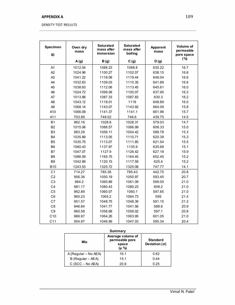
APPENDIX A 109
DENSITY TEST RESULTS
Vimal N. Patel
Specimen
ID
Oven dry mass
Saturated mass after immersion
Saturated mass after
boiling
Apparent mass
Volume of permeable pore space
(%) A (g) B (g) C (g) D (g)
A1 1012.04 1088.23 1088.8 630.22 16.7
A2 1024.96 1100.27 1102.07 638.15 16.6
A3 1041.22 1118.08 1119.44 648.04 16.6
A4 1032.63 1109.03 1110.35 641.89 16.6
A5 1038.63 1112.06 1113.45 645.61 16.0
A6 1024.72 1099.58 1100.07 637.95 16.3
A7 1013.88 1087.33 1087.83 630.3 16.2
A8 1043.12 1118.01 1118 648.89 16.0
A9 1068.14 1143.07 1143.92 664.09 15.8
A10 1066.09 1141.37 1141.1 661.96 15.7
A11 703.89 749.02 748.6 439.75 14.5
B1 962.16 1028.8 1028.31 579.03 14.7
B2 1015.06 1088.57 1086.99 608.33 15.0
B3 983.29 1056.11 1054.42 588.78 15.3
B4 1035.89 1113.05 1110.71 620.39 15.3
B5 1035.75 1113.07 1111.85 621.54 15.5
B6 1060.43 1137.97 1135.9 635.69 15.1
B7 1047.07 1127.9 1126.42 627.18 15.9
B8 1086.59 1165.75 1164.45 652.45 15.2
B9 1042.89 1120.15 1117.59 625.4 15.2
B10 1243.53 1325.72 1325.08 747.77 14.1
C1 714.27 785.36 785.43 442.75 20.8
C2 956.36 1050.19 1050.97 593.45 20.7
C3 964.2 1060.89 1061.09 599.05 21.0
C4 981.17 1080.43 1080.23 609.2 21.0
C5 962.89 1060.07 1060.1 597.85 21.0
C6 965.23 1065.2 1064.73 599 21.4
C7 951.57 1048.75 1048.39 591.15 21.2
C8 946.84 1041.77 1041.56 588.6 20.9
C9 960.58 1056.68 1056.02 597.1 20.8
C10 966.97 1064.26 1063.95 601.05 21.0
C11 954.97 1046.99 1047.03 595.34 20.4
Summary
Mix
Average volume of permeable pore
space (μ %)
Standard Deviation (σ)
A (Regular – No AEA) 16.1 0.62
B (Regular – AEA) 15.1 0.44
C (SCC – No AEA) 20.9 0.25
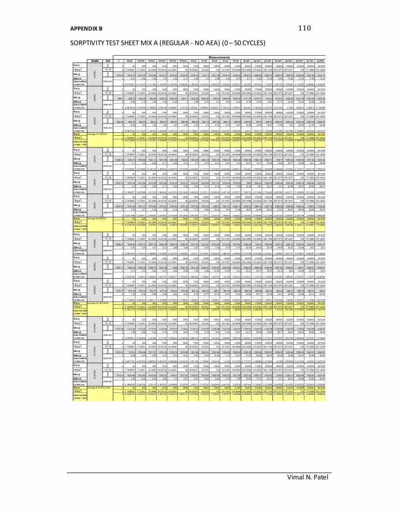
APPENDIX B 110
SORPTIVITY TEST SHEET MIX A (REGULAR - NO AEA) (0 – 50 CYCLES)
Vimal N. Patel
Samples Area 0 60s±2s 5min±10s 10min±2 20min±2 30min±2 60min±2 2hrs±5 3hrs±5 4hrs±5 5hrs±5 6hrs±5 day 1±2h day 2±2h day 3±2h day 4±2h day 5±2h day 6±2h day 7±2h day 8±2h
Time (s)
Dia
.
0 60 300 600 1200 1800 3600 7200 10800 14400 18000 21600 86400 172800 259200 345600 432000 518400 604800 691200
√Time (s½) 101.36 0 7.7459667 17.32051 24.4949 34.64102 42.42641 60 84.85281 103.923 120 134.1641 146.9694 293.9388 415.6922 509.1169 587.8775 657.2671 720 777.6889 831.3844
Mass (g)
Are
a
1013.8 1014.41 1014.72 1014.86 1015.17 1015.42 1015.97 1016.75 1017.3 1017.76 1018.15 1018.54 1023.51 1026.32 1028.12 1028.79 1029.75 1030.83 1031.63 1033.12
ΔMass (g) 0 0.61 0.92 1.06 1.37 1.62 2.17 2.95 3.5 3.96 4.35 4.74 9.71 12.52 14.32 14.99 15.95 17.03 17.83 19.32
Δmass/ areaXdensit
y of water (mm) 0 0.0755972 0.114015 0.131366 0.169784 0.200766 0.268928 0.365593 0.433754 0.490762 0.539095 0.587427 1.203359 1.551602 1.774675 1.857708 1.976681 2.110525 2.209669 2.394325
Time (s)
Dia
.
0 60 300 600 1200 1800 3600 7200 10800 14400 18000 21600 86400 172800 259200 345600 432000 518400 604800 691200
√Time (s½) 101.36 0 7.7459667 17.32051 24.4949 34.64102 42.42641 60 84.85281 103.923 120 134.1641 146.9694 293.9388 415.6922 509.1169 587.8775 657.2671 720 777.6889 831.3844
Mass (g)
Are
a
998.1 998.75 999.26 999.59 1000.03 1000.36 1001.1 1002.08 1002.85 1003.5 1004.04 1004.55 1011.45 1015.71 1018.4 1019.21 1020.34 1021.34 1022.05 1023.38
ΔMass (g) 0 0.65 1.16 1.49 1.93 2.26 3 3.98 4.75 5.4 5.94 6.45 13.35 17.61 20.3 21.11 22.24 23.24 23.95 25.28
Δmass/ areaXdensit
y of water (mm) 0 0.0805544 0.143759 0.184655 0.239185 0.280081 0.37179 0.493241 0.588667 0.669221 0.736143 0.799347 1.654463 2.182405 2.515776 2.616159 2.7562 2.88013 2.96812 3.132946
Time (s)
Dia
.
0 60 300 600 1200 1800 3600 7200 10800 14400 18000 21600 86400 172800 259200 345600 432000 518400 604800 691200
√Time (s½) 101.36 0 7.7459667 17.32051 24.4949 34.64102 42.42641 60 84.85281 103.923 120 134.1641 146.9694 293.9388 415.6922 509.1169 587.8775 657.2671 720 777.6889 831.3844
Mass (g)
Are
a
982.94 983.43 983.84 984.2 984.57 984.91 985.58 986.49 987.14 987.66 988.12 988.55 993.92 997.5 999.91 1000.87 1002.24 1003.42 1004.35 1005.79
ΔMass (g) 0 0.49 0.9 1.26 1.63 1.97 2.64 3.55 4.2 4.72 5.18 5.61 10.98 14.56 16.97 17.93 19.3 20.48 21.41 22.85
Δmass/ areaXdensit
y of water (mm) 0 0.0607256 0.111537 0.156152 0.202006 0.244142 0.327175 0.439951 0.520505 0.584949 0.641957 0.695246 1.36075 1.804419 2.103089 2.222062 2.391846 2.538083 2.653338 2.831797
Time (s) Average A1-A3(W0) 0 60 300 600 1200 1800 3600 7200 10800 14400 18000 21600 86400 172800 259200 345600 432000 518400 604800 691200
√Time (s½) 0 7.7459667 17.32051 24.4949 34.64102 42.42641 60 84.85281 103.923 120 134.1641 146.9694 293.9388 415.6922 509.1169 587.8775 657.2671 720 777.6889 831.3844
0 0.0722924 0.123104 0.157391 0.203658 0.241663 0.322631 0.432928 0.514309 0.581644 0.639065 0.694007 1.406191 1.846142 2.13118 2.231976 2.374909 2.509579 2.610376 2.786356
Time (s)
Dia
.
0 60 300 600 1200 1800 3600 7200 10800 14400 18000 21600 86400 172800 259200 345600 432000 518400 604800 691200
√Time (s½) 101.36 0 7.7459667 17.32051 24.4949 34.64102 42.42641 60 84.85281 103.923 120 134.1641 146.9694 293.9388 415.6922 509.1169 587.8775 657.2671 720 777.6889 831.3844
Mass (g)
Are
a
1048.45 1050.15 1050.65 1051.13 1051.56 1051.89 1052.6 1053.55 1054.18 1054.76 1055.26 1055.68 1060.96 1064.16 1066.71 1067.7 1069.22 1070.53 1071.55 1073.33
ΔMass (g) 0 1.7 2.2 2.68 3.11 3.44 4.15 5.1 5.73 6.31 6.81 7.23 12.51 15.71 18.26 19.25 20.77 22.08 23.1 24.88
Δmass/ areaXdensit
y of water (mm) 0 0.2106807 0.272646 0.332132 0.385422 0.426319 0.514309 0.632042 0.710118 0.781997 0.843962 0.896013 1.550362 1.946938 2.262959 2.385649 2.574023 2.736371 2.862779 3.083374
Time (s)
Dia
.
0 60 300 600 1200 1800 3600 7200 10800 14400 18000 21600 86400 172800 259200 345600 432000 518400 604800 691200
√Time (s½) 101.36 0 7.7459667 17.32051 24.4949 34.64102 42.42641 60 84.85281 103.923 120 134.1641 146.9694 293.9388 415.6922 509.1169 587.8775 657.2671 720 777.6889 831.3844
Mass (g)
Are
a
1010.72 1012.32 1012.88 1013.28 1013.83 1014.25 1015.01 1016.07 1016.83 1017.47 1018.04 1018.55 1025 1029.42 1032.93 1034.02 1035.28 1036.19 1036.63 1037.63
ΔMass (g) 0 1.6 2.16 2.56 3.11 3.53 4.29 5.35 6.11 6.75 7.32 7.83 14.28 18.7 22.21 23.3 24.56 25.47 25.91 26.91
Δmass/ areaXdensit
y of water (mm) 0 0.1982877 0.267688 0.31726 0.385422 0.437472 0.531659 0.663025 0.757211 0.836526 0.907166 0.970371 1.769718 2.317488 2.752482 2.887565 3.043717 3.156493 3.211022 3.334952
Time (s)
Dia
.
0 60 300 600 1200 1800 3600 7200 10800 14400 18000 21600 86400 172800 259200 345600 432000 518400 604800 691200
√Time (s½) 101.36 0 7.7459667 17.32051 24.4949 34.64102 42.42641 60 84.85281 103.923 120 134.1641 146.9694 293.9388 415.6922 509.1169 587.8775 657.2671 720 777.6889 831.3844
Mass (g)
Are
a
1070.47 1072.34 1073.17 1073.65 1074.27 1074.63 1075.43 1077.66 1079.43 1080.5 1081.37 1082.13 1089.54 1094.16 1097.19 1098.08 1098.88 1099.42 1099.4 1100.28
ΔMass (g) 0 1.87 2.7 3.18 3.8 4.16 4.96 7.19 8.96 10.03 10.9 11.66 19.07 23.69 26.72 27.61 28.41 28.95 28.93 29.81
Δmass/ areaXdensit
y of water (mm) 0 0.2317488 0.334611 0.394097 0.470933 0.515548 0.614692 0.891056 1.110411 1.243016 1.350835 1.445022 2.363342 2.935898 3.311405 3.421703 3.520847 3.587769 3.58529 3.694349
Time (s) Average A4-A6(T0) 0 60 300 600 1200 1800 3600 7200 10800 14400 18000 21600 86400 172800 259200 345600 432000 518400 604800 691200
√Time (s½) 0 7.7459667 17.32051 24.4949 34.64102 42.42641 60 84.85281 103.923 120 134.1641 146.9694 293.9388 415.6922 509.1169 587.8775 657.2671 720 777.6889 831.3844
0 0.2135724 0.291648 0.34783 0.413926 0.45978 0.553553 0.728707 0.859247 0.953847 1.033988 1.103802 1.894474 2.400108 2.775615 2.898306 3.046196 3.160211 3.219697 3.370892
Time (s)
Dia
.
0 60 300 600 1200 1800 3600 7200 10800 14400 18000 21600 86400 172800 259200 345600 432000 518400 604800 691200
√Time (s½) 101.36 0 7.7459667 17.32051 24.4949 34.64102 42.42641 60 84.85281 103.923 120 134.1641 146.9694 293.9388 415.6922 509.1169 587.8775 657.2671 720 777.6889 831.3844
Mass (g)
Are
a
1006.07 1006.62 1007.31 1007.74 1008.28 1008.75 1009.75 1011.34 1012.61 1013.69 1014.85 1015.83 1028.46 1030.5 1030.86 1030.16 1030.34 1030.43 1030.57 1031.37
ΔMass (g) 0 0.55 1.24 1.67 2.21 2.68 3.68 5.27 6.54 7.62 8.78 9.76 22.39 24.43 24.79 24.09 24.27 24.36 24.5 25.3
Δmass/ areaXdensit
y of water (mm) 0 0.0681614 0.153673 0.206963 0.273885 0.332132 0.456062 0.65311 0.810501 0.944345 1.088104 1.209555 2.774789 3.027606 3.072221 2.98547 3.007777 3.018931 3.036281 3.135425
Time (s)
Dia
.
0 60 300 600 1200 1800 3600 7200 10800 14400 18000 21600 86400 172800 259200 345600 432000 518400 604800 691200
√Time (s½) 101.36 0 7.7459667 17.32051 24.4949 34.64102 42.42641 60 84.85281 103.923 120 134.1641 146.9694 293.9388 415.6922 509.1169 587.8775 657.2671 720 777.6889 831.3844
Mass (g)
Are
a
1023.11 1025.24 1026.25 1026.73 1027.48 1028 1029.19 1031.06 1032.47 1033.63 1034.66 1035.61 1046.32 1048.28 1048.64 1047.83 1048.01 1048.1 1048.27 1049.01
ΔMass (g) 0 2.13 3.14 3.62 4.37 4.89 6.08 7.95 9.36 10.52 11.55 12.5 23.21 25.17 25.53 24.72 24.9 24.99 25.16 25.9
Δmass/ areaXdensit
y of water (mm) 0 0.2639706 0.38914 0.448626 0.541573 0.606017 0.753493 0.985242 1.159983 1.303742 1.43139 1.549123 2.876412 3.119314 3.163929 3.063546 3.085853 3.097007 3.118075 3.209783
Time (s)
Dia
.
0 60 300 600 1200 1800 3600 7200 10800 14400 18000 21600 86400 172800 259200 345600 432000 518400 604800 691200
√Time (s½) 101.36 0 7.7459667 17.32051 24.4949 34.64102 42.42641 60 84.85281 103.923 120 134.1641 146.9694 293.9388 415.6922 509.1169 587.8775 657.2671 720 777.6889 831.3844
Mass (g)
Are
a
973.77 975.16 976.13 976.75 977.63 978.41 979.99 982.53 984.54 986.3 987.84 989.29 998.66 998.88 999.26 998.49 998.72 998.76 998.91 999.6
ΔMass (g) 0 1.39 2.36 2.98 3.86 4.64 6.22 8.76 10.77 12.53 14.07 15.52 24.89 25.11 25.49 24.72 24.95 24.99 25.14 25.83
Δmass/ areaXdensit
y of water (mm) 0 0.1722625 0.292474 0.369311 0.478369 0.575034 0.770844 1.085625 1.334724 1.552841 1.743693 1.923391 3.084614 3.111878 3.158972 3.063546 3.09205 3.097007 3.115596 3.201108
Time (s) Average A7-A9 (W50) 0 60 300 600 1200 1800 3600 7200 10800 14400 18000 21600 86400 172800 259200 345600 432000 518400 604800 691200
√Time (s½) 0 7.7459667 17.32051 24.4949 34.64102 42.42641 60 84.85281 103.923 120 134.1641 146.9694 293.9388 415.6922 509.1169 587.8775 657.2671 720 777.6889 831.3844
0 0.1681315 0.278429 0.341633 0.431276 0.504394 0.660133 0.907993 1.101736 1.266976 1.421062 1.56069 2.911938 3.086266 3.131707 3.03752 3.061893 3.070982 3.089984 3.182105
Time (s)
Dia
.
0 60 300 600 1200 1800 3600 7200 10800 14400 18000 21600 86400 172800 259200 345600 432000 518400 604800 691200
√Time (s½) 101.36 0 7.7459667 17.32051 24.4949 34.64102 42.42641 60 84.85281 103.923 120 134.1641 146.9694 293.9388 415.6922 509.1169 587.8775 657.2671 720 777.6889 831.3844
Mass (g)
Are
a
1110.36 1112.34 1113.22 1113.78 1114.49 1115.15 1116.4 1118.14 1119.55 1120.86 1121.98 1122.97 1134.57 1139.75 1140.39 1139.49 1139.79 1139.8 1139.99 1140.81
ΔMass (g) 0 1.98 2.86 3.42 4.13 4.79 6.04 7.78 9.19 10.5 11.62 12.61 24.21 29.39 30.03 29.13 29.43 29.44 29.63 30.45
Δmass/ areaXdensit
y of water (mm) 0 0.2453811 0.354439 0.42384 0.51183 0.593624 0.748536 0.964174 1.138915 1.301263 1.440065 1.562755 3.000341 3.642298 3.721613 3.610076 3.647255 3.648495 3.672041 3.773664
Time (s)
Dia
.
0 60 300 600 1200 1800 3600 7200 10800 14400 18000 21600 86400 172800 259200 345600 432000 518400 604800 691200
√Time (s½) 101.36 0 7.7459667 17.32051 24.4949 34.64102 42.42641 60 84.85281 103.923 120 134.1641 146.9694 293.9388 415.6922 509.1169 587.8775 657.2671 720 777.6889 831.3844
Mass (g)
Are
a
1013.42 1015.5 1016.66 1017.37 1018.16 1018.75 1019.99 1021.66 1022.91 1023.94 1024.82 1025.63 1035.35 1039.24 1039.87 1039.07 1039.28 1039.33 1039.51 1040.27
ΔMass (g) 0 2.08 3.24 3.95 4.74 5.33 6.57 8.24 9.49 10.52 11.4 12.21 21.93 25.82 26.45 25.65 25.86 25.91 26.09 26.85
Δmass/ areaXdensit
y of water (mm) 0 0.2577741 0.401533 0.489523 0.587427 0.660546 0.814219 1.021182 1.176094 1.303742 1.4128 1.513183 2.717781 3.199869 3.277944 3.1788 3.204826 3.211022 3.23333 3.327516
Time (s)
Dia
.
0 60 300 600 1200 1800 3600 7200 10800 14400 18000 21600 86400 172800 259200 345600 432000 518400 604800 691200
√Time (s½) 101.36 0 7.7459667 17.32051 24.4949 34.64102 42.42641 60 84.85281 103.923 120 134.1641 146.9694 293.9388 415.6922 509.1169 587.8775 657.2671 720 777.6889 831.3844
Mass (g)
Are
a
1013.4 1014.89 1015.42 1015.83 1016.32 1016.7 1017.67 1018.67 1019.43 1020.04 1020.59 1021.09 1027.02 1030.77 1033.67 1034.8 1036.13 1036.46 1036.83 1037.65
ΔMass (g) 0 1.49 2.02 2.43 2.92 3.3 4.27 5.27 6.03 6.64 7.19 7.69 13.62 17.37 20.27 21.4 22.73 23.06 23.43 24.25
Δmass/ areaXdensit
y of water (mm) 0 0.1846555 0.250338 0.30115 0.361875 0.408968 0.52918 0.65311 0.747297 0.822894 0.891056 0.95302 1.687924 2.152661 2.512058 2.652099 2.816925 2.857822 2.903676 3.005299
Time (s) Average A10-A12 (T50) 0 60 300 600 1200 1800 3600 7200 10800 14400 18000 21600 86400 172800 259200 345600 432000 518400 604800 691200
√Time (s½) 0 7.7459667 17.32051 24.4949 34.64102 42.42641 60 84.85281 103.923 120 134.1641 146.9694 293.9388 415.6922 509.1169 587.8775 657.2671 720 777.6889 831.3844
0 0.2292702 0.335437 0.404837 0.487044 0.554379 0.697312 0.879489 1.020769 1.142633 1.247974 1.342986 2.468682 2.998276 3.170538 3.146992 3.223002 3.239113 3.269682 3.368826
Δmass/ area/ densit
y of water = 1 (mm)
Δmass/ area/ densit
y of water = 1 (mm)
Δmass/ area/ densit
y of water = 1 (mm)
8069.081
A9
(W50
)
8069.081
Δmass/ area/ densit
y of water = 1 (mm)
8069.081
8069.081
8069.081
A1
0(T
50)
A1
1(T
50)
A
12(T
50)
A8
(W50
)
8069.081
8069.081
8069.081
8069.081
A4
(T0
) A
5(T
0)
A6
(T0
) A
7(W
50
) A
1(W
0)
Measurements
A2
(W0)
A3
(W0)
8069.081
8069.081
8069.081
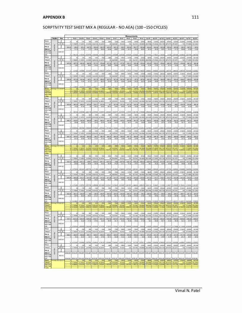
APPENDIX B 111
SORPTIVITY TEST SHEET MIX A (REGULAR - NO AEA) (100 –150 CYCLES)
Vimal N. Patel
Samples Area 0 60s±2s 5min±10s 10min±2 20min±2 30min±2 60min±2 2hrs±5 3hrs±5 4hrs±5 5hrs±5 6hrs±5 day 1±2h day 2±2h day 3±2h day 4±2h day 5±2h day 6±2h day 7±2h day 8±2h
Time (s)
Dia
.
0 60 300 600 1200 1800 3600 7200 10800 14400 18000 21600 86400 172800 259200 345600 432000 518400 604800 691200
√Time (s½) 101.36 0 7.745967 17.32051 24.4949 34.64102 42.42641 60 84.85281 103.923 120 134.1641 146.9694 293.9388 415.6922 509.1169 587.8775 657.2671 720 777.6889 831.3844
Mass (g)
Are
a
924.45 936.2 941.8 945.75 950.83 952.78 952.91 953.12 953.5 953.62 953.77 953.86 954.64 954.94 955.06 955.24 955.58 955.4 955.74 955.9
ΔMass (g) 0 11.75 17.35 21.3 26.38 28.33 28.46 28.67 29.05 29.17 29.32 29.41 30.19 30.49 30.61 30.79 31.13 30.95 31.29 31.45
Δmass/ areaXd
ensityof water
(mm) 0 1.456176 2.150183 2.639706 3.269269 3.510932 3.527043 3.553069 3.600162 3.615034 3.633623 3.644777 3.741442 3.778621 3.793492 3.8158 3.857936 3.835629 3.877765 3.897594
Time (s)
Dia
.
0 60 300 600 1200 1800 3600 7200 10800 14400 18000 21600 86400 172800 259200 345600 432000 518400 604800 691200
√Time (s½) 101.36 0 7.745967 17.32051 24.4949 34.64102 42.42641 60 84.85281 103.923 120 134.1641 146.9694 293.9388 415.6922 509.1169 587.8775 657.2671 720 777.6889 831.3844
Mass (g)
Are
a
947.89 957.72 963.02 966.56 971.31 974.44 977.52 977.77 977.97 978.11 978.38 978.44 979.35 979.41 979.61 980.03 979.91 979.89 980.18 980.38
ΔMass (g) 0 9.83 15.13 18.67 23.42 26.55 29.63 29.88 30.08 30.22 30.49 30.55 31.46 31.52 31.72 32.14 32.02 32 32.29 32.49
Δmass/ areaXd
ensityof water
(mm) 0 1.21823 1.875059 2.31377 2.902437 3.290337 3.672041 3.703024 3.72781 3.74516 3.778621 3.786057 3.898833 3.906269 3.931055 3.983105 3.968234 3.965755 4.001695 4.026481
Time (s)
Dia
.
0 60 300 600 1200 1800 3600 7200 10800 14400 18000 21600 86400 172800 259200 345600 432000 518400 604800 691200
√Time (s½) 101.36 0 7.745967 17.32051 24.4949 34.64102 42.42641 60 84.85281 103.923 120 134.1641 146.9694 293.9388 415.6922 509.1169 587.8775 657.2671 720 777.6889 831.3844
Mass (g)
Are
a
928.08 937.56 943.44 947.2 951.79 954.87 957.01 957.24 957.44 957.73 957.8 957.84 958.76 959.02 959.29 959.31 959.45 959.67 959.79 959.99
ΔMass (g) 0 9.48 15.36 19.12 23.71 26.79 28.93 29.16 29.36 29.65 29.72 29.76 30.68 30.94 31.21 31.23 31.37 31.59 31.71 31.91
Δmass/ areaXd
ensityof water
(mm) 0 1.174855 1.903562 2.369539 2.938377 3.32008 3.58529 3.613794 3.63858 3.67452 3.683195 3.688152 3.802168 3.834389 3.86785 3.870329 3.887679 3.914944 3.929815 3.954601
Time (s) Average A13-A15(W100) 0 60 300 600 1200 1800 3600 7200 10800 14400 18000 21600 86400 172800 259200 345600 432000 518400 604800 691200
√Time (s½) 0 7.745967 17.32051 24.4949 34.64102 42.42641 60 84.85281 103.923 120 134.1641 146.9694 293.9388 415.6922 509.1169 587.8775 657.2671 720 777.6889 831.3844
0 1.283087 1.976268 2.441005 3.036694 3.373783 3.594792 3.623296 3.655517 3.678238 3.69848 3.706329 3.814147 3.83976 3.864133 3.889745 3.904616 3.905442 3.936425 3.959558
Time (s)
Dia
.
0 60 300 600 1200 1800 3600 7200 10800 14400 18000 21600 86400 172800 259200 345600 432000 518400 604800 691200
√Time (s½) 101.36 0 7.745967 17.32051 24.4949 34.64102 42.42641 60 84.85281 103.923 120 134.1641 146.9694 293.9388 415.6922 509.1169 587.8775 657.2671 720 777.6889 831.3844
Mass (g)
Are
a
947.68 962.22 969.51 973.68 976.71 977.05 977 977.09 977.34 977.76 978.36 978.34 979.12 979.55 979.65 980.25 980.2 979.76 979.96 980.18
ΔMass (g) 0 14.54 21.83 26 29.03 29.37 29.32 29.41 29.66 30.08 30.68 30.66 31.44 31.87 31.97 32.57 32.52 32.08 32.28 32.5
Δmass/ areaXd
ensityof water
(mm) 0 1.80194 2.705388 3.222176 3.597683 3.639819 3.633623 3.644777 3.675759 3.72781 3.802168 3.799689 3.896354 3.949644 3.962037 4.036395 4.030198 3.975669 4.000455 4.02772
Time (s)
Dia
.
0 60 300 600 1200 1800 3600 7200 10800 14400 18000 21600 86400 172800 259200 345600 432000 518400 604800 691200
√Time (s½) 101.36 0 7.745967 17.32051 24.4949 34.64102 42.42641 60 84.85281 103.923 120 134.1641 146.9694 293.9388 415.6922 509.1169 587.8775 657.2671 720 777.6889 831.3844
Mass (g)
Are
a
896.77 916.81 926.36 928.29 929.2 929.51 930.35 930.22 930.27 930.88 931.37 931.66 932.61 932.54 932.5 932.52 932.74 932.94 933.14 933.67
ΔMass (g) 0 20.04 29.59 31.52 32.43 32.74 33.58 33.45 33.5 34.11 34.6 34.89 35.84 35.77 35.73 35.75 35.97 36.17 36.37 36.9
Δmass/ areaXd
ensityof water
(mm) 0 2.483554 3.667084 3.906269 4.019045 4.057463 4.161564 4.145453 4.15165 4.227247 4.287973 4.323912 4.441646 4.43297 4.428013 4.430492 4.457756 4.482542 4.507328 4.573011
Time (s)
Dia
.
0 60 300 600 1200 1800 3600 7200 10800 14400 18000 21600 86400 172800 259200 345600 432000 518400 604800 691200
√Time (s½) 101.36 0 7.745967 17.32051 24.4949 34.64102 42.42641 60 84.85281 103.923 120 134.1641 146.9694 293.9388 415.6922 509.1169 587.8775 657.2671 720 777.6889 831.3844
Mass (g)
Are
a
853.19 875.31 883.08 883.94 884.7 884.78 885.25 885.23 886.45 887.14 886.85 887.15 887.69 888.16 888.11 888.6 888.82 888.92 890.05 890.22
ΔMass (g) 0 22.12 29.89 30.75 31.51 31.59 32.06 32.04 33.26 33.95 33.66 33.96 34.5 34.97 34.92 35.41 35.63 35.73 36.86 37.03
Δmass/ areaXd
ensityof water
(mm) 0 2.741328 3.704263 3.810843 3.905029 3.914944 3.973191 3.970712 4.121907 4.207418 4.171479 4.208657 4.27558 4.333827 4.32763 4.388356 4.41562 4.428013 4.568054 4.589122
Time (s) Average A16-A18(T100) 0 60 300 600 1200 1800 3600 7200 10800 14400 18000 21600 86400 172800 259200 345600 432000 518400 604800 691200
√Time (s½) 0 7.745967 17.32051 24.4949 34.64102 42.42641 60 84.85281 103.923 120 134.1641 146.9694 293.9388 415.6922 509.1169 587.8775 657.2671 720 777.6889 831.3844
0 2.342274 3.358912 3.646429 3.840586 3.870742 3.922793 3.920314 3.983105 4.054158 4.087206 4.110753 4.204526 4.238814 4.239227 4.285081 4.301192 4.295408 4.358613 4.396618
Time (s)
Dia
.
0 60 300 600 1200 1800 3600 7200 10800 14400 18000 21600 86400 172800 259200 345600 432000 518400 604800 691200
√Time (s½) 101.36 0 7.745967 17.32051 24.4949 34.64102 42.42641 60 84.85281 103.923 120 134.1641 146.9694 293.9388 415.6922 509.1169 587.8775 657.2671 720 777.6889 831.3844
Mass (g)
Are
a
970.73 995.55 1005.12 1006.7 1006.81 1007.12 1007.52 1008 1007.84 1008.15 1008.34 1008.34 1009.43 1009.95 1010.49 1010.41 1010.58 1010.55 1011.08 1011.29
ΔMass (g) 0 24.82 34.39 35.97 36.08 36.39 36.79 37.27 37.11 37.42 37.61 37.61 38.7 39.22 39.76 39.68 39.85 39.82 40.35 40.56
Δmass/ areaXd
ensityof water
(mm) 0 3.075939 4.261947 4.457756 4.471389 4.509807 4.559379 4.618865 4.599036 4.637455 4.661001 4.661001 4.796085 4.860528 4.927451 4.917536 4.938604 4.934886 5.000569 5.026594
Time (s)
Dia
.
0 60 300 600 1200 1800 3600 7200 10800 14400 18000 21600 86400 172800 259200 345600 432000 518400 604800 691200
√Time (s½) 101.36 0 7.745967 17.32051 24.4949 34.64102 42.42641 60 84.85281 103.923 120 134.1641 146.9694 293.9388 415.6922 509.1169 587.8775 657.2671 720 777.6889 831.3844
Mass (g)
Are
a
870.79 906.08 912.11 911.44 911.02 911.24 911.26 911.77 910.46 910.18 910.22 910.25 911.33 911.7 912.13 912.17 912.38 912.39 912.37 912.6
ΔMass (g) 0 35.29 41.32 40.65 40.23 40.45 40.47 40.98 39.67 39.39 39.43 39.46 40.54 40.91 41.34 41.38 41.59 41.6 41.58 41.81
Δmass/ areaXd
ensityof water
(mm) 0 4.373484 5.120781 5.037748 4.985698 5.012962 5.015441 5.078645 4.916297 4.881597 4.886554 4.890272 5.024116 5.06997 5.12326 5.128217 5.154242 5.155481 5.153003 5.181507
Time (s)
Dia
.
0 60 300 600 1200 1800 3600 7200 10800 14400 18000 21600 86400 172800 259200 345600 432000 518400 604800 691200
√Time (s½) 101.36 0 7.745967 17.32051 24.4949 34.64102 42.42641 60 84.85281 103.923 120 134.1641 146.9694 293.9388 415.6922 509.1169 587.8775 657.2671 720 777.6889 831.3844
Mass (g)
Are
a
952.39 983.14 994.57 994 993.8 993.75 993.92 994.54 993.88 994.07 994.26 994.2 995.59 996.21 996.6 996.9 996.71 996.71 997.12 997.57
ΔMass (g) 0 30.75 42.18 41.61 41.41 41.36 41.53 42.15 41.49 41.68 41.87 41.81 43.2 43.82 44.21 44.51 44.32 44.32 44.73 45.18
Δmass/ areaXd
ensityof water
(mm) 0 3.810843 5.227361 5.156721 5.131935 5.125738 5.146806 5.223643 5.141849 5.165396 5.188943 5.181507 5.353769 5.430606 5.478938 5.516117 5.492571 5.492571 5.543382 5.59915
Time (s) Average A19-A21(W150) 0 60 300 600 1200 1800 3600 7200 10800 14400 18000 21600 86400 172800 259200 345600 432000 518400 604800 691200
√Time (s½) 0 7.745967 17.32051 24.4949 34.64102 42.42641 60 84.85281 103.923 120 134.1641 146.9694 293.9388 415.6922 509.1169 587.8775 657.2671 720 777.6889 831.3844
0 3.753422 4.87003 4.884075 4.863007 4.882836 4.907209 4.973718 4.885728 4.894816 4.912166 4.910927 5.05799 5.120368 5.17655 5.18729 5.195139 5.194313 5.232318 5.269084
Time (s)
Dia
.
0 60 300 600 1200 1800 3600 7200 10800 14400 18000 21600 86400 172800 259200 345600 432000 518400 604800 691200
√Time (s½) 101.36 0 7.745967 17.32051 24.4949 34.64102 42.42641 60 84.85281 103.923 120 134.1641 146.9694 293.9388 415.6922 509.1169 587.8775 657.2671 720 777.6889 831.3844
Mass (g)
Are
a
1011.5 1044.08 1059.76 1059.45 1058.73 1057.75 1057.54 1057.67 1057.85 1059.76 1058.33 1058.82 1060.1 1060.46 1060.67 1060.86 1060.88 1060.83 1060.28 1060.67
ΔMass (g) 0 32.58 48.26 47.95 47.23 46.25 46.04 46.17 46.35 48.26 46.83 47.32 48.6 48.96 49.17 49.36 49.38 49.33 48.78 49.17
Δmass/ areaXd
ensityof water
(mm) 0 4.037634 5.980854 5.942436 5.853206 5.731755 5.70573 5.721841 5.744148 5.980854 5.803635 5.86436 6.02299 6.067605 6.09363 6.117177 6.119656 6.113459 6.045298 6.09363
Time (s)
Dia
.
0 60 300 600 1200 1800 3600 7200 10800 14400 18000 21600 86400 172800 259200 345600 432000 518400 604800 691200
√Time (s½) 101.36 0 7.745967 17.32051 24.4949 34.64102 42.42641 60 84.85281 103.923 120 134.1641 146.9694 293.9388 415.6922 509.1169 587.8775 657.2671 720 777.6889 831.3844
Mass (g)
Are
a
866.41 898.81 908.82 909.11 908.81 908.33 908.57 908.87 909.85 909.29 909.32 909.01 910.03 910.79 911.26 911.38 911.79 911.78 912.08 912.43
ΔMass (g) 0 32.4 42.41 42.7 42.4 41.92 42.16 42.46 43.44 42.88 42.91 42.6 43.62 44.38 44.85 44.97 45.38 45.37 45.67 46.02
Δmass/ areaXd
ensityof water
(mm) 0 4.015327 5.255865 5.291804 5.254625 5.195139 5.224882 5.262061 5.383512 5.314112 5.31783 5.279411 5.40582 5.500006 5.558253 5.573125 5.623936 5.622697 5.659876 5.703251
Time (s)
Dia
.
0 60 300 600 1200 1800 3600 7200 10800 14400 18000 21600 86400 172800 259200 345600 432000 518400 604800 691200
√Time (s½) #DIV/0! 0 7.745967 17.32051 24.4949 34.64102 42.42641 60 84.85281 103.923 120 134.1641 146.9694 293.9388 415.6922 509.1169 587.8775 657.2671 720 777.6889 831.3844
Mass (g)
Are
a
- - - - - - - - - - - - - - - - - - - -
ΔMass (g) #VALUE! #VALUE! #VALUE! #VALUE! #VALUE! #VALUE! #VALUE! #VALUE! #VALUE! #VALUE! #VALUE! #VALUE! #VALUE! #VALUE! #VALUE! #VALUE! #VALUE! #VALUE! #VALUE! #VALUE!
Δmass/ areaXd
ensityof water
(mm) #VALUE! #VALUE! #VALUE! #VALUE! #VALUE! #VALUE! #VALUE! #VALUE! #VALUE! #VALUE! #VALUE! #VALUE! #VALUE! #VALUE! #VALUE! #VALUE! #VALUE! #VALUE! #VALUE! #VALUE!
Time (s) Average A22-A23(T150) 0 60 300 600 1200 1800 3600 7200 10800 14400 18000 21600 86400 172800 259200 345600 432000 518400 604800 691200
√Time (s½) 0 7.745967 17.32051 24.4949 34.64102 42.42641 60 84.85281 103.923 120 134.1641 146.9694 293.9388 415.6922 509.1169 587.8775 657.2671 720 777.6889 831.3844
0 4.026481 5.618359 5.61712 5.553916 5.463447 5.465306 5.491951 5.56383 5.647483 5.560732 5.571886 5.714405 5.783806 5.825942 5.845151 5.871796 5.868078 5.852587 5.898441
8069.081
A1
5(W
100
)
8069.081
Δmass/ area/ d
ensityof water
= 1 (mm)
A1
3(W
100
)
8069.081
A1
4(W
100
)
8069.081
8069.081
8069.081
A2
1(W
150
)
8069.081
Δmass/ area/ d
ensityof water
= 1 (mm)
A1
6(T
100
)
8069.081
A1
7(T
100
)
8069.081
A1
8(T
100
)A
24(T
150
)
#DIV/0!
A1
9(W
150
)
8069.081
A2
0(W
150
)
Δmass/ area/ d
ensityof water
= 1 (mm)
Δmass/ area/ d
ensityof water
= 1 (mm)
A2
2(T
150
)
8069.081
A2
3(T
150
)
Measurments
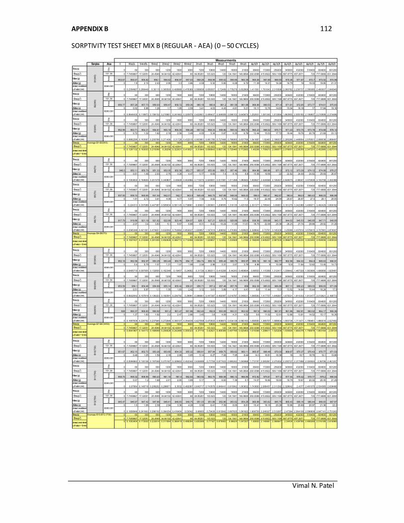
APPENDIX B 112
SORPTIVITY TEST SHEET MIX B (REGULAR - AEA) (0 – 50 CYCLES)
Vimal N. Patel
Samples Area 0 60s±2s 5min±10s 10min±2 20min±2 30min±2 60min±2 2hrs±5 3hrs±5 4hrs±5 5hrs±5 6hrs±5 day 1±2h day 2±2h day 3±2h day 4±2h day 5±2h day 6±2h day 7±2h day 8±2h
Time (s)
Dia
.
0 60 300 600 1200 1800 3600 7200 10800 14400 18000 21600 86400 172800 259200 345600 432000 518400 604800 691200
√Time (s½) 101.36 0 7.7459667 17.32051 24.4949 34.64102 42.42641 60 84.85281 103.923 120 134.1641 146.9694 293.9388 415.6922 509.1169 587.8775 657.2671 720 777.6889 831.3844
Mass (g)
Are
a
953.67 955.57 955.82 956.1 956.62 956.97 957.53 958.26 958.99 959.52 959.95 960.39 965.06 967.88 969.93 970.46 971.67 972.7 973.52 974.98
ΔMass (g) 0 1.9 2.15 2.43 2.95 3.3 3.86 4.59 5.32 5.85 6.28 6.72 11.39 14.21 16.26 16.79 18 19.03 19.85 21.31
Δmass/ areaXdensit
y of water (mm) 0 0.2354667 0.266449 0.30115 0.365593 0.408968 0.478369 0.568838 0.659307 0.72499 0.778279 0.832809 1.411561 1.761043 2.015099 2.080782 2.230737 2.358385 2.460007 2.640945
Time (s)
Dia
.
0 60 300 600 1200 1800 3600 7200 10800 14400 18000 21600 86400 172800 259200 345600 432000 518400 604800 691200
√Time (s½) 101.36 0 7.7459667 17.32051 24.4949 34.64102 42.42641 60 84.85281 103.923 120 134.1641 146.9694 293.9388 415.6922 509.1169 587.8775 657.2671 720 777.6889 831.3844
Mass (g)
Are
a
956.77 957.29 957.73 958.03 958.47 958.72 959.36 960.18 960.8 961.2 961.58 961.98 966.88 969.53 971.4 971.81 972.95 973.77 974.61 975.93
ΔMass (g) 0 0.52 0.96 1.26 1.7 1.95 2.59 3.41 4.03 4.43 4.81 5.21 10.11 12.76 14.63 15.04 16.18 17 17.84 19.16
Δmass/ areaXdensit
y of water (mm) 0 0.0644435 0.118973 0.156152 0.210681 0.241663 0.320978 0.422601 0.499437 0.549009 0.596103 0.645674 1.252931 1.581345 1.813094 1.863905 2.005185 2.106807 2.210908 2.374496
Time (s)
Dia
.
0 60 300 600 1200 1800 3600 7200 10800 14400 18000 21600 86400 172800 259200 345600 432000 518400 604800 691200
√Time (s½) 101.36 0 7.7459667 17.32051 24.4949 34.64102 42.42641 60 84.85281 103.923 120 134.1641 146.9694 293.9388 415.6922 509.1169 587.8775 657.2671 720 777.6889 831.3844
Mass (g)
Are
a
952.99 953.71 954.31 954.61 955.18 955.55 956.48 957.54 958.33 958.86 959.34 959.75 965.43 968.52 970.71 971.43 972.75 973.78 974.68 976.12
ΔMass (g) 0 0.72 1.32 1.62 2.19 2.56 3.49 4.55 5.34 5.87 6.35 6.76 12.44 15.53 17.72 18.44 19.76 20.79 21.69 23.13
Δmass/ areaXdensit
y of water (mm) 0 0.0892295 0.163587 0.200766 0.271406 0.31726 0.432515 0.563881 0.661785 0.727468 0.786955 0.837766 1.541687 1.92463 2.196037 2.285266 2.448854 2.576501 2.688038 2.866497
Time (s) Average B1-B3(W0) 0 60 300 600 1200 1800 3600 7200 10800 14400 18000 21600 86400 172800 259200 345600 432000 518400 604800 691200
√Time (s½) 0 7.7459667 17.32051 24.4949 34.64102 42.42641 60 84.85281 103.923 120 134.1641 146.9694 293.9388 415.6922 509.1169 587.8775 657.2671 720 777.6889 831.3844
0 0.1297132 0.183003 0.219356 0.28256 0.322631 0.410621 0.51844 0.606843 0.667156 0.720445 0.772083 1.40206 1.755673 2.008077 2.076651 2.228259 2.347231 2.452985 2.627313
Time (s)
Dia
.
0 60 300 600 1200 1800 3600 7200 10800 14400 18000 21600 86400 172800 259200 345600 432000 518400 604800 691200
√Time (s½) 101.36 0 7.7459667 17.32051 24.4949 34.64102 42.42641 60 84.85281 103.923 120 134.1641 146.9694 293.9388 415.6922 509.1169 587.8775 657.2671 720 777.6889 831.3844
Mass (g)
Are
a
949.3 950.11 950.79 951.33 952.05 952.58 953.77 955.07 955.99 956.7 957.46 958.1 964.88 968.86 971.3 972.12 973.39 974.12 974.99 976.27
ΔMass (g) 0 0.81 1.49 2.03 2.75 3.28 4.47 5.77 6.69 7.4 8.16 8.8 15.58 19.56 22 22.82 24.09 24.82 25.69 26.97
Δmass/ areaXdensit
y of water (mm) 0 0.1003832 0.184655 0.251578 0.340807 0.40649 0.553966 0.715075 0.829091 0.917081 1.011268 1.090583 1.930827 2.424068 2.726457 2.828079 2.98547 3.075939 3.183758 3.342388
Time (s)
Dia
.
0 60 300 600 1200 1800 3600 7200 10800 14400 18000 21600 86400 172800 259200 345600 432000 518400 604800 691200
√Time (s½) 101.36 0 7.7459667 17.32051 24.4949 34.64102 42.42641 60 84.85281 103.923 120 134.1641 146.9694 293.9388 415.6922 509.1169 587.8775 657.2671 720 777.6889 831.3844
Mass (g)
Are
a
937.93 939.74 940.65 941.54 942.01 942.7 943.9 945.49 946.75 947.69 948.55 949.43 956.5 960.41 962.87 963.6 964.9 965.43 966.03 966.98
ΔMass (g) 0 1.81 2.72 3.61 4.08 4.77 5.97 7.56 8.82 9.76 10.62 11.5 18.57 22.48 24.94 25.67 26.97 27.5 28.1 29.05
Δmass/ areaXdensit
y of water (mm) 0 0.224313 0.337089 0.447387 0.505634 0.591145 0.739861 0.93691 1.093061 1.209555 1.316135 1.425193 2.301377 2.785943 3.09081 3.181279 3.342388 3.408071 3.482429 3.600162
Time (s)
Dia
.
0 60 300 600 1200 1800 3600 7200 10800 14400 18000 21600 86400 172800 259200 345600 432000 518400 604800 691200
√Time (s½) 101.36 0 7.7459667 17.32051 24.4949 34.64102 42.42641 60 84.85281 103.923 120 134.1641 146.9694 293.9388 415.6922 509.1169 587.8775 657.2671 720 777.6889 831.3844
Mass (g)
Are
a
917.79 919.86 921.19 921.62 922.89 923.46 924.67 926.1 927.21 928.03 928.88 929.4 936.58 939.88 943.17 944.02 945.53 946.65 947.71 949.05
ΔMass (g) 0 2.07 3.4 3.83 5.1 5.67 6.88 8.31 9.42 10.24 11.09 11.61 18.79 22.09 25.38 26.23 27.74 28.86 29.92 31.26
Δmass/ areaXdensit
y of water (mm) 0 0.2565348 0.421361 0.474651 0.632042 0.702682 0.852637 1.029857 1.167419 1.269042 1.374382 1.438825 2.328642 2.73761 3.145339 3.25068 3.437814 3.576615 3.707981 3.874047
Time (s) Average B4-B6(T0) 0 60 300 600 1200 1800 3600 7200 10800 14400 18000 21600 86400 172800 259200 345600 432000 518400 604800 691200
√Time (s½) 0 7.7459667 17.32051 24.4949 34.64102 42.42641 60 84.85281 103.923 120 134.1641 146.9694 293.9388 415.6922 509.1169 587.8775 657.2671 720 777.6889 831.3844
0 0.1937437 0.314369 0.391205 0.492828 0.566772 0.715488 0.893947 1.029857 1.131893 1.233928 1.3182 2.186949 2.649207 2.987535 3.086679 3.255224 3.353542 3.458056 3.605532
Time (s)
Dia
.
0 60 300 600 1200 1800 3600 7200 10800 14400 18000 21600 86400 172800 259200 345600 432000 518400 604800 691200
√Time (s½) 101.36 0 7.7459667 17.32051 24.4949 34.64102 42.42641 60 84.85281 103.923 120 134.1641 146.9694 293.9388 415.6922 509.1169 587.8775 657.2671 720 777.6889 831.3844
Mass (g)
Are
a
952.18 952.58 952.97 953.25 953.49 953.75 954.17 954.74 955.16 955.49 955.75 955.97 959.16 961.18 962.77 962.98 964.02 964.8 965.63 966.91
ΔMass (g) 0 0.4 0.79 1.07 1.31 1.57 1.99 2.56 2.98 3.31 3.57 3.79 6.98 9 10.59 10.8 11.84 12.62 13.45 14.73
Δmass/ areaXdensit
y of water (mm) 0 0.0495719 0.097905 0.132605 0.162348 0.19457 0.24662 0.31726 0.369311 0.410208 0.44243 0.469694 0.86503 1.115369 1.312417 1.338442 1.467329 1.563995 1.666856 1.825487
Time (s)
Dia
.
0 60 300 600 1200 1800 3600 7200 10800 14400 18000 21600 86400 172800 259200 345600 432000 518400 604800 691200
√Time (s½) 101.36 0 7.7459667 17.32051 24.4949 34.64102 42.42641 60 84.85281 103.923 120 134.1641 146.9694 293.9388 415.6922 509.1169 587.8775 657.2671 720 777.6889 831.3844
Mass (g)
Are
a
953.59 954.1 954.46 954.69 955.14 955.42 956.01 956.71 957.2 957.48 957.76 958 962.39 965.03 966.89 967.11 968.23 969.03 969.83 971.09
ΔMass (g) 0 0.51 0.87 1.1 1.55 1.83 2.42 3.12 3.61 3.89 4.17 4.41 8.8 11.44 13.3 13.52 14.64 15.44 16.24 17.5
Δmass/ areaXdensit
y of water (mm) 0 0.0632042 0.107819 0.136323 0.192091 0.226792 0.29991 0.386661 0.447387 0.482087 0.516787 0.546531 1.090583 1.417757 1.648267 1.675531 1.814333 1.913477 2.012621 2.168772
Time (s)
Dia
.
0 60 300 600 1200 1800 3600 7200 10800 14400 18000 21600 86400 172800 259200 345600 432000 518400 604800 691200
√Time (s½) 101.36 0 7.7459667 17.32051 24.4949 34.64102 42.42641 60 84.85281 103.923 120 134.1641 146.9694 293.9388 415.6922 509.1169 587.8775 657.2671 720 777.6889 831.3844
Mass (g)
Are
a
949 950.37 950.83 950.92 951.2 951.47 951.86 952.45 952.8 953.09 953.31 953.52 957.8 960.02 961.91 961.86 962.81 963.52 964.17 965.36
ΔMass (g) 0 1.37 1.83 1.92 2.2 2.47 2.86 3.45 3.8 4.09 4.31 4.52 8.8 11.02 12.91 12.86 13.81 14.52 15.17 16.36
Δmass/ areaXdensit
y of water (mm) 0 0.1697839 0.226792 0.237945 0.272646 0.306107 0.354439 0.427558 0.470933 0.506873 0.534138 0.560163 1.090583 1.365707 1.599934 1.593738 1.711471 1.799461 1.880016 2.027492
Time (s) Average B7-B9 (W50) 0 60 300 600 1200 1800 3600 7200 10800 14400 18000 21600 86400 172800 259200 345600 432000 518400 604800 691200
√Time (s½) 0 7.7459667 17.32051 24.4949 34.64102 42.42641 60 84.85281 103.923 120 134.1641 146.9694 293.9388 415.6922 509.1169 587.8775 657.2671 720 777.6889 831.3844
0 0.0941867 0.144172 0.168958 0.209028 0.242489 0.300323 0.37716 0.42921 0.466389 0.497785 0.525463 1.015399 1.299611 1.520206 1.535904 1.664378 1.758978 1.853164 2.00725
Time (s)
Dia
.
0 60 300 600 1200 1800 3600 7200 10800 14400 18000 21600 86400 172800 259200 345600 432000 518400 604800 691200
√Time (s½) 101.36 0 7.7459667 17.32051 24.4949 34.64102 42.42641 60 84.85281 103.923 120 134.1641 146.9694 293.9388 415.6922 509.1169 587.8775 657.2671 720 777.6889 831.3844
Mass (g)
Are
a
951.67 952.15 952.72 953.26 953.85 954.33 955.32 956.81 957.94 958.75 959.62 960.11 965.97 968.48 970.03 969.67 970.37 970.43 970.77 971.53
ΔMass (g) 0 0.48 1.05 1.59 2.18 2.66 3.65 5.14 6.27 7.08 7.95 8.44 14.3 16.81 18.36 18 18.7 18.76 19.1 19.86
Δmass/ areaXdensit
y of water (mm) 0 0.0594863 0.130126 0.197048 0.270167 0.329653 0.452344 0.636999 0.77704 0.877423 0.985242 1.045968 1.772197 2.083261 2.275352 2.230737 2.317488 2.324924 2.36706 2.461247
Time (s)
Dia
.
0 60 300 600 1200 1800 3600 7200 10800 14400 18000 21600 86400 172800 259200 345600 432000 518400 604800 691200
√Time (s½) 101.36 0 7.7459667 17.32051 24.4949 34.64102 42.42641 60 84.85281 103.923 120 134.1641 146.9694 293.9388 415.6922 509.1169 587.8775 657.2671 720 777.6889 831.3844
Mass (g)
Are
a
958.75 959.32 959.95 960.43 961.16 961.6 962.64 963.92 964.75 965.58 966.14 966.85 972.82 975.61 977.4 977.54 978.42 978.77 979.2 980.04
ΔMass (g) 0 0.57 1.2 1.68 2.41 2.85 3.89 5.17 6 6.83 7.39 8.1 14.07 16.86 18.65 18.79 19.67 20.02 20.45 21.29
Δmass/ areaXdensit
y of water (mm) 0 0.07064 0.148716 0.208202 0.298671 0.3532 0.482087 0.640717 0.743579 0.846441 0.915842 1.003832 1.743693 2.089457 2.311292 2.328642 2.4377 2.481075 2.534365 2.638466
Time (s)
Dia
.
0 60 300 600 1200 1800 3600 7200 10800 14400 18000 21600 86400 172800 259200 345600 432000 518400 604800 691200
√Time (s½) 101.36 0 7.7459667 17.32051 24.4949 34.64102 42.42641 60 84.85281 103.923 120 134.1641 146.9694 293.9388 415.6922 509.1169 587.8775 657.2671 720 777.6889 831.3844
Mass (g)
Are
a
945.47 946.97 947.42 947.86 948.41 948.83 949.75 951.03 951.88 952.86 953.52 954.28 960.88 963.62 965.75 965.43 966.16 966.44 966.83 967.67
ΔMass (g) 0 1.5 1.95 2.39 2.94 3.36 4.28 5.56 6.41 7.39 8.05 8.81 15.41 18.15 20.28 19.96 20.69 20.97 21.36 22.2
Δmass/ areaXdensit
y of water (mm) 0 0.1858948 0.241663 0.296192 0.364354 0.416404 0.53042 0.68905 0.79439 0.915842 0.997635 1.091822 1.909759 2.249327 2.513297 2.47364 2.564108 2.598809 2.647141 2.751243
Time (s) Average B10-B12 (T50) 0 60 300 600 1200 1800 3600 7200 10800 14400 18000 21600 86400 172800 259200 345600 432000 518400 604800 691200
√Time (s½) 0 7.7459667 17.32051 24.4949 34.64102 42.42641 60 84.85281 103.923 120 134.1641 146.9694 293.9388 415.6922 509.1169 587.8775 657.2671 720 777.6889 831.3844
0 0.1053404 0.173502 0.233814 0.311064 0.366419 0.488284 0.655589 0.77167 0.879902 0.96624 1.047207 1.80855 2.140681 2.366647 2.34434 2.439766 2.468269 2.516189 2.616985
B7
(W50
) B
8(W
50
)B
9(W
50
)
Measurments
B2
(W0)
B3
(W0)
8069.081
8069.081
8069.081
8069.081
Δmass/ area/ densit
y of water = 1 (mm)
Δmass/ area/ densit
y of water = 1 (mm)
Δmass/ area/ densit
y of water = 1 (mm)
8069.081
8069.081
B1
0(T
50)
8069.081
8069.081
8069.081
8069.081
8069.081
8069.081
B1
1(T
50)
B
12(T
50)
Δmass/ area/ densit
y of water = 1 (mm)
B1
(W0)
B4
(T0
) B
5(T
0)
B6
(T0
)
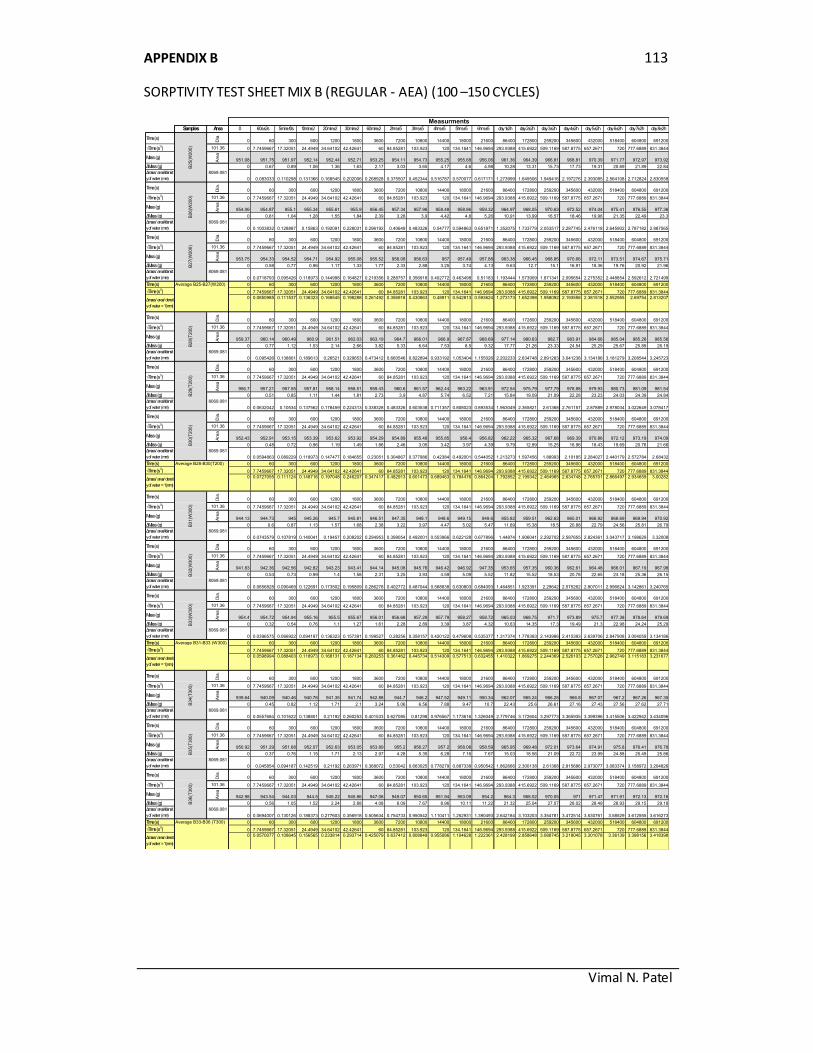
APPENDIX B 113
SORPTIVITY TEST SHEET MIX B (REGULAR - AEA) (100 –150 CYCLES)
Vimal N. Patel
Samples Area 0 60s±2s 5min±10s 10min±2 20min±2 30min±2 60min±2 2hrs±5 3hrs±5 4hrs±5 5hrs±5 6hrs±5 day 1±2h day 2±2h day 3±2h day 4±2h day 5±2h day 6±2h day 7±2h day 8±2h
Time (s)
Dia
.
0 60 300 600 1200 1800 3600 7200 10800 14400 18000 21600 86400 172800 259200 345600 432000 518400 604800 691200
√Time (s½) 101.36 0 7.7459667 17.32051 24.4949 34.64102 42.42641 60 84.85281 103.923 120 134.1641 146.9694 293.9388 415.6922 509.1169 587.8775 657.2671 720 777.6889 831.3844
Mass (g)
Are
a
951.08 951.75 951.97 952.14 952.44 952.71 953.25 954.11 954.73 955.25 955.68 956.06 961.36 964.39 966.81 968.81 970.39 971.77 972.97 973.92
ΔMass (g) 0 0.67 0.89 1.06 1.36 1.63 2.17 3.03 3.65 4.17 4.6 4.98 10.28 13.31 15.73 17.73 19.31 20.69 21.89 22.84
Δmass/ areaXdensit
y of water (mm) 0 0.083033 0.110298 0.131366 0.168545 0.202006 0.268928 0.375507 0.452344 0.516787 0.570077 0.617171 1.273999 1.649506 1.949416 2.197276 2.393085 2.564108 2.712824 2.830558
Time (s)
Dia
.
0 60 300 600 1200 1800 3600 7200 10800 14400 18000 21600 86400 172800 259200 345600 432000 518400 604800 691200
√Time (s½) 101.36 0 7.7459667 17.32051 24.4949 34.64102 42.42641 60 84.85281 103.923 120 134.1641 146.9694 293.9388 415.6922 509.1169 587.8775 657.2671 720 777.6889 831.3844
Mass (g)
Are
a
954.06 954.87 955.1 955.34 955.61 955.9 956.45 957.34 957.96 958.48 958.86 959.32 964.97 968.05 970.63 972.52 974.04 975.41 976.55 977.36
ΔMass (g) 0 0.81 1.04 1.28 1.55 1.84 2.39 3.28 3.9 4.42 4.8 5.26 10.91 13.99 16.57 18.46 19.98 21.35 22.49 23.3
Δmass/ areaXdensit
y of water (mm) 0 0.1003832 0.128887 0.15863 0.192091 0.228031 0.296192 0.40649 0.483326 0.54777 0.594863 0.651871 1.352075 1.733779 2.053517 2.287745 2.476118 2.645902 2.787182 2.887565
Time (s)
Dia
.
0 60 300 600 1200 1800 3600 7200 10800 14400 18000 21600 86400 172800 259200 345600 432000 518400 604800 691200
√Time (s½) 101.36 0 7.7459667 17.32051 24.4949 34.64102 42.42641 60 84.85281 103.923 120 134.1641 146.9694 293.9388 415.6922 509.1169 587.8775 657.2671 720 777.6889 831.3844
Mass (g)
Are
a
953.75 954.33 954.52 954.71 954.92 955.08 955.52 956.08 956.63 957 957.49 957.88 963.38 966.45 968.85 970.66 972.11 973.51 974.67 975.71
ΔMass (g) 0 0.58 0.77 0.96 1.17 1.33 1.77 2.33 2.88 3.25 3.74 4.13 9.63 12.7 15.1 16.91 18.36 19.76 20.92 21.96
Δmass/ areaXdensit
y of water (mm) 0 0.0718793 0.095426 0.118973 0.144998 0.164827 0.219356 0.288757 0.356918 0.402772 0.463498 0.51183 1.193444 1.573909 1.871341 2.095654 2.275352 2.448854 2.592612 2.721499
Time (s) Average B25-B27(W200) 0 60 300 600 1200 1800 3600 7200 10800 14400 18000 21600 86400 172800 259200 345600 432000 518400 604800 691200
√Time (s½) 0 7.7459667 17.32051 24.4949 34.64102 42.42641 60 84.85281 103.923 120 134.1641 146.9694 293.9388 415.6922 509.1169 587.8775 657.2671 720 777.6889 831.3844
0 0.0850985 0.111537 0.136323 0.168545 0.198288 0.261492 0.356918 0.430863 0.48911 0.542813 0.593624 1.273173 1.652398 1.958092 2.193558 2.381518 2.552955 2.69754 2.813207
Time (s)
Dia
.
0 60 300 600 1200 1800 3600 7200 10800 14400 18000 21600 86400 172800 259200 345600 432000 518400 604800 691200
√Time (s½) 101.36 0 7.7459667 17.32051 24.4949 34.64102 42.42641 60 84.85281 103.923 120 134.1641 146.9694 293.9388 415.6922 509.1169 587.8775 657.2671 720 777.6889 831.3844
Mass (g)
Are
a
959.37 960.14 960.49 960.9 961.51 962.03 963.19 964.7 966.01 966.9 967.87 968.69 977.14 980.63 982.7 983.91 984.66 985.04 985.26 985.56
ΔMass (g) 0 0.77 1.12 1.53 2.14 2.66 3.82 5.33 6.64 7.53 8.5 9.32 17.77 21.26 23.33 24.54 25.29 25.67 25.89 26.19
Δmass/ areaXdensit
y of water (mm) 0 0.095426 0.138801 0.189613 0.26521 0.329653 0.473412 0.660546 0.822894 0.933192 1.053404 1.155026 2.202233 2.634748 2.891283 3.041238 3.134186 3.181279 3.208544 3.245723
Time (s)
Dia
.
0 60 300 600 1200 1800 3600 7200 10800 14400 18000 21600 86400 172800 259200 345600 432000 518400 604800 691200
√Time (s½) 101.36 0 7.7459667 17.32051 24.4949 34.64102 42.42641 60 84.85281 103.923 120 134.1641 146.9694 293.9388 415.6922 509.1169 587.8775 657.2671 720 777.6889 831.3844
Mass (g)
Are
a
956.7 957.21 957.55 957.81 958.14 958.51 959.43 960.6 961.57 962.44 963.22 963.91 972.54 975.79 977.79 978.98 979.93 980.73 981.09 981.54
ΔMass (g) 0 0.51 0.85 1.11 1.44 1.81 2.73 3.9 4.87 5.74 6.52 7.21 15.84 19.09 21.09 22.28 23.23 24.03 24.39 24.84
Δmass/ areaXdensit
y of water (mm) 0 0.0632042 0.10534 0.137562 0.178459 0.224313 0.338328 0.483326 0.603538 0.711357 0.808023 0.893534 1.963049 2.365821 2.61368 2.761157 2.87889 2.978034 3.022649 3.078417
Time (s)
Dia
.
0 60 300 600 1200 1800 3600 7200 10800 14400 18000 21600 86400 172800 259200 345600 432000 518400 604800 691200
√Time (s½) 101.36 0 7.7459667 17.32051 24.4949 34.64102 42.42641 60 84.85281 103.923 120 134.1641 146.9694 293.9388 415.6922 509.1169 587.8775 657.2671 720 777.6889 831.3844
Mass (g)
Are
a
952.43 952.91 953.15 953.39 953.62 953.92 954.29 954.89 955.48 955.85 956.4 956.82 962.22 965.32 967.68 969.39 970.86 972.12 973.19 974.09
ΔMass (g) 0 0.48 0.72 0.96 1.19 1.49 1.86 2.46 3.05 3.42 3.97 4.39 9.79 12.89 15.25 16.96 18.43 19.69 20.76 21.66
Δmass/ areaXdensit
y of water (mm) 0 0.0594863 0.089229 0.118973 0.147477 0.184655 0.23051 0.304867 0.377986 0.42384 0.492001 0.544052 1.213273 1.597456 1.88993 2.10185 2.284027 2.440179 2.572784 2.68432
Time (s) Average B28-B30(T200) 0 60 300 600 1200 1800 3600 7200 10800 14400 18000 21600 86400 172800 259200 345600 432000 518400 604800 691200
√Time (s½) 0 7.7459667 17.32051 24.4949 34.64102 42.42641 60 84.85281 103.923 120 134.1641 146.9694 293.9388 415.6922 509.1169 587.8775 657.2671 720 777.6889 831.3844
0 0.0727055 0.111124 0.148716 0.197048 0.246207 0.347417 0.482913 0.601473 0.689463 0.784476 0.864204 1.792852 2.199342 2.464965 2.634748 2.765701 2.866497 2.934659 3.00282
Time (s)
Dia
.
0 60 300 600 1200 1800 3600 7200 10800 14400 18000 21600 86400 172800 259200 345600 432000 518400 604800 691200
√Time (s½) 101.36 0 7.7459667 17.32051 24.4949 34.64102 42.42641 60 84.85281 103.923 120 134.1641 146.9694 293.9388 415.6922 509.1169 587.8775 657.2671 720 777.6889 831.3844
Mass (g)
Are
a
944.13 944.73 945 945.26 945.7 945.81 946.51 947.35 948.1 948.6 949.15 949.6 955.82 959.51 962.63 965.01 966.92 968.69 969.94 970.92
ΔMass (g) 0 0.6 0.87 1.13 1.57 1.68 2.38 3.22 3.97 4.47 5.02 5.47 11.69 15.38 18.5 20.88 22.79 24.56 25.81 26.79
Δmass/ areaXdensit
y of water (mm) 0 0.0743579 0.107819 0.140041 0.19457 0.208202 0.294953 0.399054 0.492001 0.553966 0.622128 0.677896 1.44874 1.906041 2.292702 2.587655 2.824361 3.043717 3.198629 3.32008
Time (s)
Dia
.
0 60 300 600 1200 1800 3600 7200 10800 14400 18000 21600 86400 172800 259200 345600 432000 518400 604800 691200
√Time (s½) 101.36 0 7.7459667 17.32051 24.4949 34.64102 42.42641 60 84.85281 103.923 120 134.1641 146.9694 293.9388 415.6922 509.1169 587.8775 657.2671 720 777.6889 831.3844
Mass (g)
Are
a
941.83 942.36 942.56 942.82 943.23 943.41 944.14 945.08 945.76 946.42 946.92 947.35 953.65 957.35 960.36 962.61 964.48 966.01 967.19 967.98
ΔMass (g) 0 0.53 0.73 0.99 1.4 1.58 2.31 3.25 3.93 4.59 5.09 5.52 11.82 15.52 18.53 20.78 22.65 24.18 25.36 26.15
Δmass/ areaXdensit
y of water (mm) 0 0.0656828 0.090469 0.122691 0.173502 0.195809 0.286278 0.402772 0.487044 0.568838 0.630803 0.684093 1.464851 1.923391 2.29642 2.575262 2.807011 2.996624 3.142861 3.240765
Time (s)
Dia
.
0 60 300 600 1200 1800 3600 7200 10800 14400 18000 21600 86400 172800 259200 345600 432000 518400 604800 691200
√Time (s½) 101.36 0 7.7459667 17.32051 24.4949 34.64102 42.42641 60 84.85281 103.923 120 134.1641 146.9694 293.9388 415.6922 509.1169 587.8775 657.2671 720 777.6889 831.3844
Mass (g)
Are
a
954.4 954.72 954.94 955.16 955.5 955.67 956.01 956.68 957.29 957.79 958.27 958.72 965.03 968.75 971.7 973.89 975.7 977.38 978.64 979.69
ΔMass (g) 0 0.32 0.54 0.76 1.1 1.27 1.61 2.28 2.89 3.39 3.87 4.32 10.63 14.35 17.3 19.49 21.3 22.98 24.24 25.29
Δmass/ areaXdensit
y of water (mm) 0 0.0396575 0.066922 0.094187 0.136323 0.157391 0.199527 0.28256 0.358157 0.420122 0.479608 0.535377 1.317374 1.778393 2.143986 2.415393 2.639706 2.847908 3.004059 3.134186
Time (s) Average B31-B33 (W300) 0 60 300 600 1200 1800 3600 7200 10800 14400 18000 21600 86400 172800 259200 345600 432000 518400 604800 691200
√Time (s½) 0 7.7459667 17.32051 24.4949 34.64102 42.42641 60 84.85281 103.923 120 134.1641 146.9694 293.9388 415.6922 509.1169 587.8775 657.2671 720 777.6889 831.3844
0 0.0598994 0.088403 0.118973 0.168131 0.187134 0.260253 0.361462 0.445734 0.514309 0.577513 0.632455 1.410322 1.869275 2.244369 2.526103 2.757026 2.962749 3.115183 3.231677
Time (s)
Dia
.
0 60 300 600 1200 1800 3600 7200 10800 14400 18000 21600 86400 172800 259200 345600 432000 518400 604800 691200
√Time (s½) 101.36 0 7.7459667 17.32051 24.4949 34.64102 42.42641 60 84.85281 103.923 120 134.1641 146.9694 293.9388 415.6922 509.1169 587.8775 657.2671 720 777.6889 831.3844
Mass (g)
Are
a
939.64 940.09 940.46 940.76 941.35 941.74 942.88 944.7 946.2 947.52 949.11 950.34 962.07 965.24 966.25 966.8 967.07 967.2 967.26 967.35
ΔMass (g) 0 0.45 0.82 1.12 1.71 2.1 3.24 5.06 6.56 7.88 9.47 10.7 22.43 25.6 26.61 27.16 27.43 27.56 27.62 27.71
Δmass/ areaXdensit
y of water (mm) 0 0.0557684 0.101622 0.138801 0.21192 0.260253 0.401533 0.627085 0.81298 0.976567 1.173616 1.326049 2.779746 3.172604 3.297773 3.365935 3.399396 3.415506 3.422942 3.434096
Time (s)
Dia
.
0 60 300 600 1200 1800 3600 7200 10800 14400 18000 21600 86400 172800 259200 345600 432000 518400 604800 691200
√Time (s½) 101.36 0 7.7459667 17.32051 24.4949 34.64102 42.42641 60 84.85281 103.923 120 134.1641 146.9694 293.9388 415.6922 509.1169 587.8775 657.2671 720 777.6889 831.3844
Mass (g)
Are
a
950.92 951.29 951.68 952.07 952.63 953.05 953.89 955.2 956.27 957.2 958.08 958.59 965.95 969.48 972.01 973.64 974.91 975.8 976.41 976.78
ΔMass (g) 0 0.37 0.76 1.15 1.71 2.13 2.97 4.28 5.35 6.28 7.16 7.67 15.03 18.56 21.09 22.72 23.99 24.88 25.49 25.86
Δmass/ areaXdensit
y of water (mm) 0 0.045854 0.094187 0.142519 0.21192 0.263971 0.368072 0.53042 0.663025 0.778279 0.887338 0.950542 1.862666 2.300138 2.61368 2.815686 2.973077 3.083374 3.158972 3.204826
Time (s)
Dia
.
0 60 300 600 1200 1800 3600 7200 10800 14400 18000 21600 86400 172800 259200 345600 432000 518400 604800 691200
√Time (s½) 101.36 0 7.7459667 17.32051 24.4949 34.64102 42.42641 60 84.85281 103.923 120 134.1641 146.9694 293.9388 415.6922 509.1169 587.8775 657.2671 720 777.6889 831.3844
Mass (g)
Are
a
942.98 943.54 944.03 944.5 945.22 945.86 947.06 949.07 950.65 951.94 953.09 954.2 964.3 968.02 970.05 971 971.47 971.91 972.13 972.16
ΔMass (g) 0 0.56 1.05 1.52 2.24 2.88 4.08 6.09 7.67 8.96 10.11 11.22 21.32 25.04 27.07 28.02 28.49 28.93 29.15 29.18
Δmass/ areaXdensit
y of water (mm) 0 0.0694007 0.130126 0.188373 0.277603 0.356918 0.505634 0.754733 0.950542 1.110411 1.252931 1.390493 2.642184 3.103203 3.354781 3.472514 3.530761 3.58529 3.612555 3.616273
Time (s) Average B33-B36 (T300) 0 60 300 600 1200 1800 3600 7200 10800 14400 18000 21600 86400 172800 259200 345600 432000 518400 604800 691200
√Time (s½) 0 7.7459667 17.32051 24.4949 34.64102 42.42641 60 84.85281 103.923 120 134.1641 146.9694 293.9388 415.6922 509.1169 587.8775 657.2671 720 777.6889 831.3844
0 0.0570077 0.108645 0.156565 0.233814 0.293714 0.425079 0.637412 0.808849 0.955086 1.104628 1.222361 2.428199 2.858648 3.088745 3.218045 3.301078 3.36139 3.398156 3.418398
B3
5(T
300
)
B3
6(T
300
) B
28(T
200
) B
29(T
200
) B
30(T
200
)
8069.081
Δmass/ area/ densit
y of water = 1 (mm)
Δmass/ area/ densit
y of water = 1 (mm)
8069.081
8069.081
B3
4(T
300
)
8069.081
8069.081
8069.081
B3
1(W
300
)
8069.081
B3
2(W
300
)B
33(W
300
)
Measurments
B2
6(W
200
)
8069.081
Δmass/ area/ densit
y of water = 1 (mm)
B2
5(W
200
)
8069.081
8069.081
8069.081
Δmass/ area/ densit
y of water = 1 (mm)
B2
7(W
200
)
8069.081
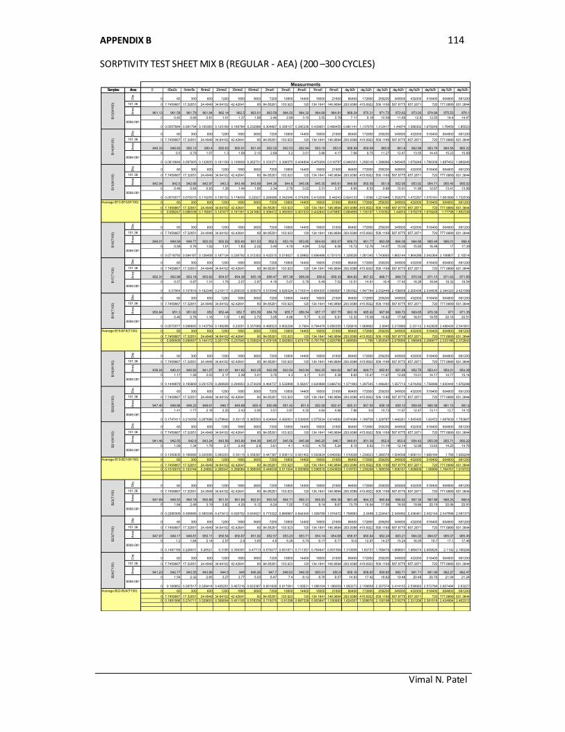
APPENDIX B 114
SORPTIVITY TEST SHEET MIX B (REGULAR - AEA) (200 –300 CYCLES)
Vimal N. Patel
Samples Area 0 60s±2s 5min±10s 10min±2 20min±2 30min±2 60min±2 2hrs±5 3hrs±5 4hrs±5 5hrs±5 6hrs±5 day 1±2h day 2±2h day 3±2h day 4±2h day 5±2h day 6±2h day 7±2h day 8±2h
Dia
.
0 60 300 600 1200 1800 3600 7200 10800 14400 18000 21600 86400 172800 259200 345600 432000 518400 604800 691200
101.36 0 7.7459667 17.32051 24.4949 34.64102 42.42641 60 84.85281 103.923 120 134.1641 146.9694 293.9388 415.6922 509.1169 587.8775 657.2671 720 777.6889 831.3844
Are
a
961.13 961.58 961.79 961.94 962.14 962.5 963.01 963.59 964.02 964.32 964.68 964.91 968.24 970.31 971.72 972.82 973.93 974.68 975.53 976.1
0 0.45 0.66 0.81 1.01 1.37 1.88 2.46 2.89 3.19 3.55 3.78 7.11 9.18 10.59 11.69 12.8 13.55 14.4 14.97
0 0.0557684 0.081794 0.100383 0.125169 0.169784 0.232988 0.304867 0.358157 0.395336 0.439951 0.468455 0.881141 1.137676 1.312417 1.44874 1.586302 1.679249 1.78459 1.85523
Dia
.0 60 300 600 1200 1800 3600 7200 10800 14400 18000 21600 86400 172800 259200 345600 432000 518400 604800 691200
101.36 0 7.7459667 17.32051 24.4949 34.64102 42.42641 60 84.85281 103.923 120 134.1641 146.9694 293.9388 415.6922 509.1169 587.8775 657.2671 720 777.6889 831.3844
Are
a
949.33 949.83 950.12 950.4 950.63 950.91 951.45 952.02 952.53 952.84 953.19 953.5 956.99 959.08 960.6 961.8 962.88 963.76 964.56 965.22
0 0.5 0.79 1.07 1.3 1.58 2.12 2.69 3.2 3.51 3.86 4.17 7.66 9.75 11.27 12.47 13.55 14.43 15.23 15.89
0 0.0619649 0.097905 0.132605 0.161109 0.195809 0.262731 0.333371 0.396575 0.434994 0.478369 0.516787 0.949303 1.208316 1.396689 1.545405 1.679249 1.788308 1.887452 1.969245
Dia
.
0 60 300 600 1200 1800 3600 7200 10800 14400 18000 21600 86400 172800 259200 345600 432000 518400 604800 691200
101.36 0 7.7459667 17.32051 24.4949 34.64102 42.42641 60 84.85281 103.923 120 134.1641 146.9694 293.9388 415.6922 509.1169 587.8775 657.2671 720 777.6889 831.3844
Are
a
942.04 942.5 942.68 942.97 943.3 943.48 943.89 944.38 944.8 945.06 945.35 945.61 948.69 950.59 951.9 952.95 953.92 954.71 955.45 956.02
0 0.46 0.64 0.93 1.26 1.44 1.85 2.34 2.76 3.02 3.31 3.57 6.65 8.55 9.86 10.91 11.88 12.67 13.41 13.98
0 0.0570077 0.079315 0.115255 0.156152 0.178459 0.22927 0.289996 0.342046 0.374268 0.410208 0.44243 0.824133 1.0596 1.221948 1.352075 1.472287 1.570191 1.661899 1.732539
Average B13-B15(W100) 0 60 300 600 1200 1800 3600 7200 10800 14400 18000 21600 86400 172800 259200 345600 432000 518400 604800 691200
0 7.7459667 17.32051 24.4949 34.64102 42.42641 60 84.85281 103.923 120 134.1641 146.9694 293.9388 415.6922 509.1169 587.8775 657.2671 720 777.6889 831.3844
0 0.058247 0.086338 0.116081 0.147477 0.181351 0.241663 0.309412 0.365593 0.401533 0.442843 0.475891 0.884859 1.135197 1.310352 1.44874 1.579279 1.679249 1.77798 1.852338
Dia
.
0 60 300 600 1200 1800 3600 7200 10800 14400 18000 21600 86400 172800 259200 345600 432000 518400 604800 691200
101.36 0 7.7459667 17.32051 24.4949 34.64102 42.42641 60 84.85281 103.923 120 134.1641 146.9694 293.9388 415.6922 509.1169 587.8775 657.2671 720 777.6889 831.3844
Are
a
949.01 949.59 949.77 950.03 950.52 950.84 951.53 952.5 953.19 953.85 954.63 955.07 959.73 961.77 963.08 964.06 964.86 965.49 966.01 966.4
0 0.58 0.76 1.02 1.51 1.83 2.52 3.49 4.18 4.84 5.62 6.06 10.72 12.76 14.07 15.05 15.85 16.48 17 17.39
0 0.0718793 0.094187 0.126408 0.187134 0.226792 0.312303 0.432515 0.518027 0.59982 0.696486 0.751015 1.328528 1.581345 1.743693 1.865144 1.964288 2.042364 2.106807 2.15514
Dia
.
0 60 300 600 1200 1800 3600 7200 10800 14400 18000 21600 86400 172800 259200 345600 432000 518400 604800 691200
101.36 0 7.7459667 17.32051 24.4949 34.64102 42.42641 60 84.85281 103.923 120 134.1641 146.9694 293.9388 415.6922 509.1169 587.8775 657.2671 720 777.6889 831.3844
Are
a
952.31 952.88 953.18 953.62 954.07 954.38 955.18 956.47 957.38 958.09 958.8 959.33 964.82 967.22 968.71 969.73 970.59 971.15 971.63 971.85
0 0.57 0.87 1.31 1.76 2.07 2.87 4.16 5.07 5.78 6.49 7.02 12.51 14.91 16.4 17.42 18.28 18.84 19.32 19.54
0 0.07064 0.107819 0.162348 0.218117 0.256535 0.355679 0.515548 0.628324 0.716314 0.804305 0.869987 1.550362 1.847794 2.032449 2.158858 2.265438 2.334838 2.394325 2.421589
Dia
.
0 60 300 600 1200 1800 3600 7200 10800 14400 18000 21600 86400 172800 259200 345600 432000 518400 604800 691200
101.36 0 7.7459667 17.32051 24.4949 34.64102 42.42641 60 84.85281 103.923 120 134.1641 146.9694 293.9388 415.6922 509.1169 587.8775 657.2671 720 777.6889 831.3844
Are
a
950.84 951.3 951.62 952 952.44 952.7 953.56 954.79 955.7 956.54 957.17 957.75 963.16 965.92 967.66 968.72 969.65 970.39 971 971.35
0 0.46 0.78 1.16 1.6 1.86 2.72 3.95 4.86 5.7 6.33 6.91 12.32 15.08 16.82 17.88 18.81 19.55 20.16 20.51
0 0.0570077 0.096665 0.143759 0.198288 0.23051 0.337089 0.489523 0.602299 0.7064 0.784476 0.856355 1.526816 1.868862 2.0845 2.215866 2.33112 2.422828 2.498426 2.541801
Average B16-B18(T100) 0 60 300 600 1200 1800 3600 7200 10800 14400 18000 21600 86400 172800 259200 345600 432000 518400 604800 691200
0 7.7459667 17.32051 24.4949 34.64102 42.42641 60 84.85281 103.923 120 134.1641 146.9694 293.9388 415.6922 509.1169 587.8775 657.2671 720 777.6889 831.3844
0 0.066509 0.099557 0.144172 0.201179 0.237945 0.335024 0.479195 0.582883 0.674178 0.761755 0.825786 1.468569 1.766 1.953547 2.079956 2.186949 2.266677 2.333186 2.372843
Dia
.
0 60 300 600 1200 1800 3600 7200 10800 14400 18000 21600 86400 172800 259200 345600 432000 518400 604800 691200
101.36 0 7.7459667 17.32051 24.4949 34.64102 42.42641 60 84.85281 103.923 120 134.1641 146.9694 293.9388 415.6922 509.1169 587.8775 657.2671 720 777.6889 831.3844
Are
a
939.24 940.41 940.82 941.27 941.41 941.62 942.25 942.99 943.54 943.94 944.25 944.62 947.89 949.71 950.91 951.89 952.75 953.41 954.01 954.38
0 1.17 1.58 2.03 2.17 2.38 3.01 3.75 4.3 4.7 5.01 5.38 8.65 10.47 11.67 12.65 13.51 14.17 14.77 15.14
0 0.1449979 0.195809 0.251578 0.268928 0.294953 0.373029 0.464737 0.532898 0.58247 0.620889 0.666743 1.071993 1.297545 1.446261 1.567713 1.674292 1.756086 1.830444 1.876298
Dia
.
0 60 300 600 1200 1800 3600 7200 10800 14400 18000 21600 86400 172800 259200 345600 432000 518400 604800 691200
101.36 0 7.7459667 17.32051 24.4949 34.64102 42.42641 60 84.85281 103.923 120 134.1641 146.9694 293.9388 415.6922 509.1169 587.8775 657.2671 720 777.6889 831.3844
Are
a
947.45 948.86 949.22 949.61 949.7 949.88 950.4 950.96 951.42 951.8 952.09 952.41 955.31 957.05 958.18 959.12 959.92 960.56 961.15 961.6
0 1.41 1.77 2.16 2.25 2.43 2.95 3.51 3.97 4.35 4.64 4.96 7.86 9.6 10.73 11.67 12.47 13.11 13.7 14.15
0 0.1747411 0.219356 0.267688 0.278842 0.30115 0.365593 0.434994 0.492001 0.539095 0.575034 0.614692 0.974089 1.189726 1.329767 1.446261 1.545405 1.62472 1.697839 1.753607
Dia
.
0 60 300 600 1200 1800 3600 7200 10800 14400 18000 21600 86400 172800 259200 345600 432000 518400 604800 691200
101.36 0 7.7459667 17.32051 24.4949 34.64102 42.42641 60 84.85281 103.923 120 134.1641 146.9694 293.9388 415.6922 509.1169 587.8775 657.2671 720 777.6889 831.3844
Are
a
941.46 942.55 942.8 943.24 943.56 943.89 944.36 945.07 945.56 945.99 946.25 946.7 949.61 951.39 952.6 953.6 954.42 955.09 955.71 956.22
0 1.09 1.34 1.78 2.1 2.43 2.9 3.61 4.1 4.53 4.79 5.24 8.15 9.93 11.14 12.14 12.96 13.63 14.25 14.76
0 0.1350835 0.166066 0.220595 0.260253 0.30115 0.359397 0.447387 0.508112 0.561402 0.593624 0.649392 1.010028 1.230623 1.380578 1.504508 1.606131 1.689164 1.766 1.829204
Average B19-B21(W150) 0 60 300 600 1200 1800 3600 7200 10800 14400 18000 21600 86400 172800 259200 345600 432000 518400 604800 691200
0 7.7459667 17.32051 24.4949 34.64102 42.42641 60 84.85281 103.923 120 134.1641 146.9694 293.9388 415.6922 509.1169 587.8775 657.2671 720 777.6889 831.3844
0 0.1516075 0.193744 0.24662 0.269341 0.299084 0.366006 0.449039 0.511004 0.560989 0.596516 0.643609 1.018703 1.239298 1.385536 1.506161 1.608609 1.68999 1.764761 1.819703
Dia
.
0 60 300 600 1200 1800 3600 7200 10800 14400 18000 21600 86400 172800 259200 345600 432000 518400 604800 691200
101.36 0 7.7459667 17.32051 24.4949 34.64102 42.42641 60 84.85281 103.923 120 134.1641 146.9694 293.9388 415.6922 509.1169 587.8775 657.2671 720 777.6889 831.3844
Are
a
947.69 949.53 950.18 950.88 951.51 951.94 952.81 953.93 954.71 955.31 955.83 956.36 961.48 964.23 965.64 966.62 967.35 967.88 968.25 968.6
0 1.84 2.49 3.19 3.82 4.25 5.12 6.24 7.02 7.62 8.14 8.67 13.79 16.54 17.95 18.93 19.66 20.19 20.56 20.91
0 0.2280309 0.308585 0.395336 0.473412 0.526702 0.634521 0.773322 0.869987 0.944345 1.008789 1.074472 1.708993 2.0498 2.224541 2.345992 2.436461 2.502144 2.547998 2.591373
Dia
.
0 60 300 600 1200 1800 3600 7200 10800 14400 18000 21600 86400 172800 259200 345600 432000 518400 604800 691200
101.36 0 7.7459667 17.32051 24.4949 34.64102 42.42641 60 84.85281 103.923 120 134.1641 146.9694 293.9388 415.6922 509.1169 587.8775 657.2671 720 777.6889 831.3844
Are
a
947.97 949.17 949.81 950.11 950.54 950.87 951.82 952.57 953.23 953.71 954.14 954.68 958.57 960.94 962.24 963.21 964.02 964.67 965.07 965.45
0 1.2 1.84 2.14 2.57 2.9 3.85 4.6 5.26 5.74 6.17 6.71 10.6 12.97 14.27 15.24 16.05 16.7 17.1 17.48
0 0.1487158 0.228031 0.26521 0.3185 0.359397 0.47713 0.570077 0.651871 0.711357 0.764647 0.831569 1.313656 1.60737 1.768479 1.888691 1.989074 2.069628 2.1192 2.166294
Dia
.
0 60 300 600 1200 1800 3600 7200 10800 14400 18000 21600 86400 172800 259200 345600 432000 518400 604800 691200
101.36 0 7.7459667 17.32051 24.4949 34.64102 42.42641 60 84.85281 103.923 120 134.1641 146.9694 293.9388 415.6922 509.1169 587.8775 657.2671 720 777.6889 831.3844
Are
a
941.23 942.77 943.55 943.88 944.5 945 946.26 947.7 948.63 949.35 950.01 950.8 956.16 958.65 959.85 960.71 961.71 961.99 962.27 962.47
0 1.54 2.32 2.65 3.27 3.77 5.03 6.47 7.4 8.12 8.78 9.57 14.93 17.42 18.62 19.48 20.48 20.76 21.04 21.24
0 0.190852 0.287517 0.328414 0.405251 0.467216 0.623367 0.801826 0.917081 1.00631 1.088104 1.186009 1.850273 2.158858 2.307574 2.414153 2.538083 2.572784 2.607484 2.63227
Average B22-B24(T150) 0 60 300 600 1200 1800 3600 7200 10800 14400 18000 21600 86400 172800 259200 345600 432000 518400 604800 691200
0 7.7459667 17.32051 24.4949 34.64102 42.42641 60 84.85281 103.923 120 134.1641 146.9694 293.9388 415.6922 509.1169 587.8775 657.2671 720 777.6889 831.3844
0 0.1891996 0.274711 0.329653 0.399054 0.451105 0.578339 0.715075 0.81298 0.887338 0.953847 1.030683 1.624307 1.938676 2.100198 2.216279 2.321206 2.381518 2.424894 2.463312
B1
3(W
100
)
Measurments
B1
4(W
100
)B
15(W
100
)
8069.081
8069.081
8069.081
B2
3(T
150
)B
24(T
150
)B
16(T
100
)B
17(T
100
)B
18(T
100
)B
19(W
150
)B
20(W
150
)B
21(W
150
)
8069.081
8069.081
8069.081
8069.081
8069.081
8069.081
8069.081
8069.081
8069.081
B2
2(T
150
)
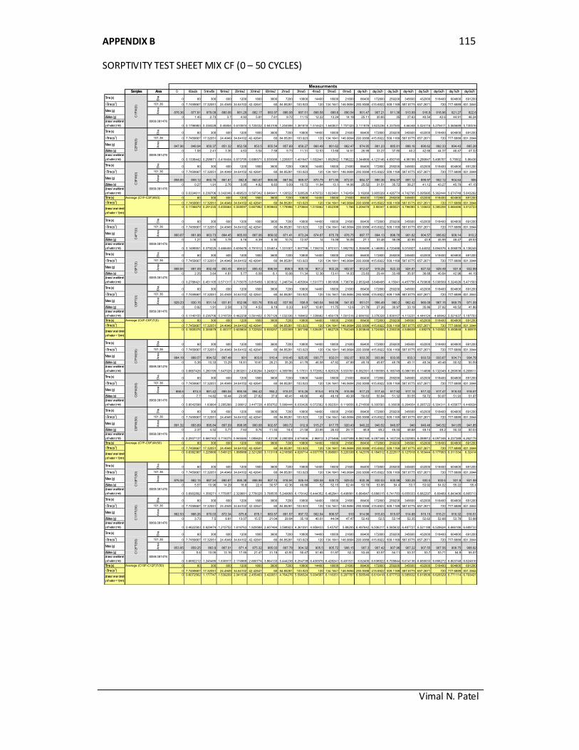
APPENDIX B 115
SORPTIVITY TEST SHEET MIX CF (0 – 50 CYCLES)
Vimal N. Patel
Samples Area 0 60s±2s 5min±10s 10min±2 20min±2 30min±2 60min±2 2hrs±5 3hrs±5 4hrs±5 5hrs±5 6hrs±5 day 1±2h day 2±2h day 3±2h day 4±2h day 5±2h day 6±2h day 7±2h day 8±2h
Time (s)
Dia
.
0 60 300 600 1200 1800 3600 7200 10800 14400 18000 21600 86400 172800 259200 345600 432000 518400 604800 691200
√Time (s½) 101.36 0 7.7459667 17.32051 24.4949 34.64102 42.42641 60 84.85281 103.923 120 134.1641 146.9694 293.9388 415.6922 509.1169 587.8775 657.2671 720 777.6889 831.3844
Mass (g)
Are
a
876.36 877.81 879.09 880.06 881.29 882.17 883.97 886.08 887.51 888.58 889.6 890.54 901.47 907.21 911.36 913.99 916.9 918.96 921.27 922.6
ΔMass (g) 0 1.45 2.73 3.7 4.93 5.81 7.61 9.72 11.15 12.22 13.24 14.18 25.11 30.85 35 37.63 40.54 42.6 44.91 46.24
Δmass/ areaXdensit
y of water (mm) 0 0.1796983 0.338328 0.45854 0.610974 0.720032 0.943106 1.204598 1.381818 1.514423 1.640831 1.757325 3.111878 3.823236 4.337545 4.66348 5.024116 5.279411 5.565689 5.730516
Time (s)
Dia
.
0 60 300 600 1200 1800 3600 7200 10800 14400 18000 21600 86400 172800 259200 345600 432000 518400 604800 691200
√Time (s½) 101.36 0 7.7459667 17.32051 24.4949 34.64102 42.42641 60 84.85281 103.923 120 134.1641 146.9694 293.9388 415.6922 509.1169 587.8775 657.2671 720 777.6889 831.3844
Mass (g)
Are
a
847.96 849.04 850.37 851.32 852.59 853.5 855.54 857.69 859.27 860.49 861.62 862.47 874.95 881.23 885.81 888.16 890.62 892.33 894.43 895.28
ΔMass (g) 0 1.08 2.41 3.36 4.63 5.54 7.58 9.73 11.31 12.53 13.66 14.51 26.99 33.27 37.85 40.2 42.66 44.37 46.47 47.32
Δmass/ areaXdensit
y of water (mm) 0 0.1338442 0.298671 0.416404 0.573795 0.686571 0.939388 1.205837 1.401647 1.552841 1.692882 1.798222 3.344866 4.123146 4.690745 4.98198 5.286847 5.498767 5.75902 5.86436
Time (s)
Dia
.
0 60 300 600 1200 1800 3600 7200 10800 14400 18000 21600 86400 172800 259200 345600 432000 518400 604800 691200
√Time (s½) 101.36 0 7.7459667 17.32051 24.4949 34.64102 42.42641 60 84.85281 103.923 120 134.1641 146.9694 293.9388 415.6922 509.1169 587.8775 657.2671 720 777.6889 831.3844
Mass (g)
Are
a
858.85 859.12 860.76 861.61 862.8 863.67 865.68 867.94 869.57 870.79 871.95 872.91 884.37 890.36 894.57 897.12 899.97 902.12 904.64 906
ΔMass (g) 0 0.27 1.91 2.76 3.95 4.82 6.83 9.09 10.72 11.94 13.1 14.06 25.52 31.51 35.72 38.27 41.12 43.27 45.79 47.15
Δmass/ areaXdensit
y of water (mm) 0 0.0334611 0.236706 0.342046 0.489523 0.597342 0.846441 1.126522 1.328528 1.479722 1.623481 1.742454 3.16269 3.905029 4.426774 4.742795 5.095995 5.362444 5.674748 5.843292
Time (s) Average (C1F-C3F)W(0) 0 60 300 600 1200 1800 3600 7200 10800 14400 18000 21600 86400 172800 259200 345600 432000 518400 604800 691200
√Time (s½) 0 7.7459667 17.32051 24.4949 34.64102 42.42641 60 84.85281 103.923 120 134.1641 146.9694 293.9388 415.6922 509.1169 587.8775 657.2671 720 777.6889 831.3844
0 0.1156679 0.291235 0.405664 0.558097 0.667982 0.909645 1.178986 1.370664 1.515662 1.652398 1.766 3.206478 3.95047 4.485021 4.796085 5.135653 5.380208 5.666486 5.812723
Time (s)
Dia
.
0 60 300 600 1200 1800 3600 7200 10800 14400 18000 21600 86400 172800 259200 345600 432000 518400 604800 691200
√Time (s½) 101.36 0 7.7459667 17.32051 24.4949 34.64102 42.42641 60 84.85281 103.923 120 134.1641 146.9694 293.9388 415.6922 509.1169 587.8775 657.2671 720 777.6889 831.3844
Mass (g)
Are
a
860.67 861.88 863.73 864.45 865.83 867.06 869.02 871.41 873.24 874.67 875.76 876.75 887.77 894.13 898.76 901.62 904.57 906.62 909.14 910.2
ΔMass (g) 0 1.21 3.06 3.78 5.16 6.39 8.35 10.74 12.57 14 15.09 16.08 27.1 33.46 38.09 40.95 43.9 45.95 48.47 49.53
Δmass/ areaXdensit
y of water (mm) 0 0.1499551 0.379225 0.468455 0.639478 0.791912 1.034814 1.331007 1.557798 1.735018 1.870101 1.992792 3.358499 4.146693 4.720488 5.074927 5.44052 5.694576 6.006879 6.138245
Time (s)
Dia
.
0 60 300 600 1200 1800 3600 7200 10800 14400 18000 21600 86400 172800 259200 345600 432000 518400 604800 691200
√Time (s½) 101.36 0 7.7459667 17.32051 24.4949 34.64102 42.42641 60 84.85281 103.923 120 134.1641 146.9694 293.9388 415.6922 509.1169 587.8775 657.2671 720 777.6889 831.3844
Mass (g)
Are
a
888.84 891.09 892.48 893.45 894.61 895.42 896.94 898.9 900.18 901.2 902.25 902.87 912.67 918.28 922.33 924.81 927.52 929.48 931.8 932.99
ΔMass (g) 0 2.25 3.64 4.61 5.77 6.58 8.1 10.06 11.34 12.36 13.41 14.03 23.83 29.44 33.49 35.97 38.68 40.64 42.96 44.15
Δmass/ areaXdensit
y of water (mm) 0 0.2788421 0.451105 0.571317 0.715075 0.815458 1.003832 1.246734 1.405364 1.531773 1.661899 1.738736 2.953248 3.648495 4.15041 4.457756 4.793606 5.036509 5.324026 5.471503
Time (s)
Dia
.
0 60 300 600 1200 1800 3600 7200 10800 14400 18000 21600 86400 172800 259200 345600 432000 518400 604800 691200
√Time (s½) 101.36 0 7.7459667 17.32051 24.4949 34.64102 42.42641 60 84.85281 103.923 120 134.1641 146.9694 293.9388 415.6922 509.1169 587.8775 657.2671 720 777.6889 831.3844
Mass (g)
Are
a
929.23 930.15 931.14 931.81 932.96 933.76 935.42 937.56 938.9 940.04 940.98 941.83 951.01 956.49 960.2 962.42 965.09 967.15 969.75 971.09
ΔMass (g) 0 0.92 1.91 2.58 3.73 4.53 6.19 8.33 9.67 10.81 11.75 12.6 21.78 27.26 30.97 33.19 35.86 37.92 40.52 41.86
Δmass/ areaXdensit
y of water (mm) 0 0.1140155 0.236706 0.319739 0.462258 0.561402 0.767126 1.032336 1.198402 1.339682 1.456176 1.561516 2.699192 3.378328 3.838107 4.113231 4.444124 4.69942 5.021637 5.187703
Time (s) Average (C4F-C6F)T(0) 0 60 300 600 1200 1800 3600 7200 10800 14400 18000 21600 86400 172800 259200 345600 432000 518400 604800 691200
√Time (s½) 0 7.7459667 17.32051 24.4949 34.64102 42.42641 60 84.85281 103.923 120 134.1641 146.9694 293.9388 415.6922 509.1169 587.8775 657.2671 720 777.6889 831.3844
0 0.1809376 0.355679 0.45317 0.605604 0.722924 0.935257 1.203359 1.387188 1.535491 1.662725 1.764348 3.003646 3.724505 4.236335 4.548638 4.89275 5.143502 5.450848 5.59915
Time (s)
Dia
.
0 60 300 600 1200 1800 3600 7200 10800 14400 18000 21600 86400 172800 259200 345600 432000 518400 604800 691200
√Time (s½) 101.36 0 7.7459667 17.32051 24.4949 34.64102 42.42641 60 84.85281 103.923 120 134.1641 146.9694 293.9388 415.6922 509.1169 587.8775 657.2671 720 777.6889 831.3844
Mass (g)
Are
a
884.19 889.57 894.52 897.48 901 903.8 910.4 919.45 925.95 930.77 932.01 932.07 933.35 933.86 933.95 933.3 933.53 933.67 934.71 934.78
ΔMass (g) 0 5.38 10.33 13.29 16.81 19.61 26.21 35.26 41.76 46.58 47.82 47.88 49.16 49.67 49.76 49.11 49.34 49.48 50.52 50.59
Δmass/ areaXdensit
y of water (mm) 0 0.6667426 1.280195 1.647028 2.083261 2.430264 3.248201 4.369766 5.17531 5.772652 5.926325 5.933761 6.092391 6.155595 6.166749 6.086195 6.114698 6.132049 6.260936 6.269611
Time (s)
Dia
.
0 60 300 600 1200 1800 3600 7200 10800 14400 18000 21600 86400 172800 259200 345600 432000 518400 604800 691200
√Time (s½) 101.36 0 7.7459667 17.32051 24.4949 34.64102 42.42641 60 84.85281 103.923 120 134.1641 146.9694 293.9388 415.6922 509.1169 587.8775 657.2671 720 777.6889 831.3844
Mass (g)
Are
a
866.6 874.3 881.42 885.04 890.55 894.42 904.2 915.01 915.26 915.6 915.76 915.98 917.23 917.44 917.92 917.15 917.32 917.47 918.53 918.57
ΔMass (g) 0 7.7 14.82 18.44 23.95 27.82 37.6 48.41 48.66 49 49.16 49.38 50.63 50.84 51.32 50.55 50.72 50.87 51.93 51.97
Δmass/ areaXdensit
y of water (mm) 0 0.9542598 1.83664 2.285266 2.96812 3.447728 4.659762 5.999444 6.030426 6.072562 6.092391 6.119656 6.274568 6.300593 6.36008 6.264654 6.285722 6.304311 6.435677 6.440634
Time (s)
Dia
.
0 60 300 600 1200 1800 3600 7200 10800 14400 18000 21600 86400 172800 259200 345600 432000 518400 604800 691200
√Time (s½) 101.36 0 7.7459667 17.32051 24.4949 34.64102 42.42641 60 84.85281 103.923 120 134.1641 146.9694 293.9388 415.6922 509.1169 587.8775 657.2671 720 777.6889 831.3844
Mass (g)
Are
a
891.32 893.69 895.84 897.09 898.95 900.08 902.87 909.72 912.9 915.27 917.75 920.43 940.22 940.52 940.87 940 940.46 940.52 941.65 941.85
ΔMass (g) 0 2.37 4.52 5.77 7.63 8.76 11.55 18.4 21.58 23.95 26.43 29.11 48.9 49.2 49.55 48.68 49.14 49.2 50.33 50.53
Δmass/ areaXdensit
y of water (mm) 0 0.2937137 0.560163 0.715075 0.945585 1.085625 1.43139 2.280309 2.674406 2.96812 3.275466 3.607598 6.060169 6.097348 6.140724 6.032905 6.089912 6.097348 6.237389 6.262175
Time (s) Average (C7F-C9F)W(50) 0 60 300 600 1200 1800 3600 7200 10800 14400 18000 21600 86400 172800 259200 345600 432000 518400 604800 691200
√Time (s½) 0 7.7459667 17.32051 24.4949 34.64102 42.42641 60 84.85281 103.923 120 134.1641 146.9694 293.9388 415.6922 509.1169 587.8775 657.2671 720 777.6889 831.3844
0 0.6382387 1.225666 1.549123 1.998988 2.321206 3.113118 4.216506 4.626714 4.937778 5.098061 5.220338 6.142376 6.184512 6.222517 6.127918 6.163444 6.177903 6.311334 6.32414
Time (s)
Dia
.
0 60 300 600 1200 1800 3600 7200 10800 14400 18000 21600 86400 172800 259200 345600 432000 518400 604800 691200
√Time (s½) 101.36 0 7.7459667 17.32051 24.4949 34.64102 42.42641 60 84.85281 103.923 120 134.1641 146.9694 293.9388 415.6922 509.1169 587.8775 657.2671 720 777.6889 831.3844
Mass (g)
Are
a
876.58 882.15 887.54 890.87 895.38 898.98 907.15 918.94 926.44 928.58 928.73 929.02 930.36 930.53 930.98 930.28 930.5 930.6 931.8 931.98
ΔMass (g) 0 5.57 10.96 14.29 18.8 22.4 30.57 42.36 49.86 52 52.15 52.44 53.78 53.95 54.4 53.7 53.92 54.02 55.22 55.4
Δmass/ areaXdensit
y of water (mm) 0 0.6902892 1.358271 1.770957 2.329881 2.776028 3.788535 5.249668 6.179142 6.444352 6.462941 6.498881 6.664947 6.686015 6.741783 6.655033 6.682297 6.69469 6.843406 6.865713
Time (s)
Dia
.
0 60 300 600 1200 1800 3600 7200 10800 14400 18000 21600 86400 172800 259200 345600 432000 518400 604800 691200
√Time (s½) 101.36 0 7.7459667 17.32051 24.4949 34.64102 42.42641 60 84.85281 103.923 120 134.1641 146.9694 293.9388 415.6922 509.1169 587.8775 657.2671 720 777.6889 831.3844
Mass (g)
Are
a
862.53 866.26 870.03 872.34 875.6 878.1 883.57 891.57 897.72 902.54 906.57 910 914.96 915.03 915.67 914.88 915.15 915.21 916.32 916.51
ΔMass (g) 0 3.73 7.5 9.81 13.07 15.57 21.04 29.04 35.19 40.01 44.04 47.47 52.43 52.5 53.14 52.35 52.62 52.68 53.79 53.98
Δmass/ areaXdensit
y of water (mm) 0 0.4622583 0.929474 1.215752 1.619763 1.929588 2.607484 3.598923 4.361091 4.958433 5.45787 5.88295 6.497642 6.506317 6.585632 6.487727 6.521188 6.528624 6.666186 6.689733
Time (s)
Dia
.
0 60 300 600 1200 1800 3600 7200 10800 14400 18000 21600 86400 172800 259200 345600 432000 518400 604800 691200
√Time (s½) 101.36 0 7.7459667 17.32051 24.4949 34.64102 42.42641 60 84.85281 103.923 120 134.1641 146.9694 293.9388 415.6922 509.1169 587.8775 657.2671 720 777.6889 831.3844
Mass (g)
Are
a
853.85 859.25 863.9 867.01 871.4 875.32 885.03 897.78 904.32 905.5 905.72 906.15 907.3 907.42 907.96 907.22 907.55 907.56 908.75 908.92
ΔMass (g) 0 5.4 10.05 13.16 17.55 21.47 31.18 43.93 50.47 51.65 51.87 52.3 53.45 53.57 54.11 53.37 53.7 53.71 54.9 55.07
Δmass/ areaXdensit
y of water (mm) 0 0.6692212 1.245495 1.630917 2.174969 2.660774 3.864133 5.444238 6.254739 6.400976 6.428241 6.481531 6.62405 6.638922 6.705844 6.614136 6.655033 6.656272 6.803748 6.824816
Time (s) Average (C10F-C12F)T(50) 0 60 300 600 1200 1800 3600 7200 10800 14400 18000 21600 86400 172800 259200 345600 432000 518400 604800 691200
√Time (s½) 0 7.7459667 17.32051 24.4949 34.64102 42.42641 60 84.85281 103.923 120 134.1641 146.9694 293.9388 415.6922 509.1169 587.8775 657.2671 720 777.6889 831.3844
0 0.6072562 1.177747 1.539209 2.041538 2.455463 3.420051 4.764276 5.598324 5.934587 6.116351 6.287787 6.595546 6.610418 6.677753 6.585632 6.619506 6.626529 6.771114 6.793421
Δmass/ area/ densit
y of water = 1 (mm)
Δmass/ area/ densit
y of water = 1 (mm)
Δmass/ area/ densit
y of water = 1 (mm)
8069.081476
C9F
W(5
0)
8069.081476
Δmass/ area/ densit
y of water = 1 (mm)
8069.081476
8069.081476
8069.081476
8069.081476
8069.081476
8069.081476
8069.081476
C10F
T(5
0)
C11F
T(5
0)
C12F
T(5
0)
C4F
T(0
)C
5F
T(0
) C
6F
T(0
) C
7F
W(5
0)
C8F
W(5
0)
C1F
W(0
)
Measurments
C2F
W(0
) C
3F
W(0
)
8069.081476
8069.081476
8069.081476
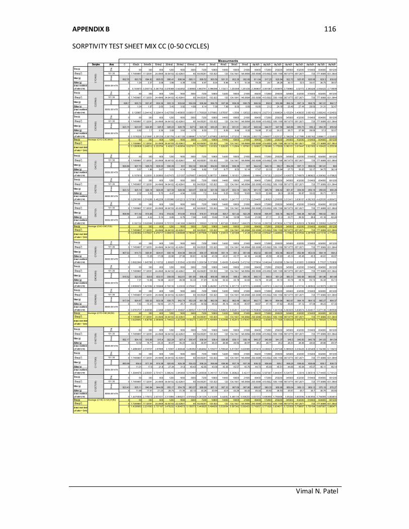
APPENDIX B 116
SORPTIVITY TEST SHEET MIX CC (0-50 CYCLES)
Vimal N. Patel
Samples Area 0 60s±2s 5min±10s 10min±2 20min±2 30min±2 60min±2 2hrs±5 3hrs±5 4hrs±5 5hrs±5 6hrs±5 day 1±2h day 2±2h day 3±2h day 4±2h day 5±2h day 6±2h day 7±2h day 8±2h
Time (s)
Dia
.
0 60 300 600 1200 1800 3600 7200 10800 14400 18000 21600 86400 172800 259200 345600 432000 518400 604800 691200
√Time (s½) 101.36 0 7.7459667 17.32051 24.4949 34.64102 42.42641 60 84.85281 103.923 120 134.1641 146.9694 293.9388 415.6922 509.1169 587.8775 657.2671 720 777.6889 831.3844
Mass (g)
Are
a
892.55 893.79 894.92 895.63 896.41 896.94 898.11 899.52 900.59 901.51 902.26 902.89 911.84 917.25 920.84 922.72 925.05 926.96 929.3 930.62
ΔMass (g) 0 1.24 2.37 3.08 3.86 4.39 5.56 6.97 8.04 8.96 9.71 10.34 19.29 24.7 28.29 30.17 32.5 34.41 36.75 38.07
Δmass/ areaXdensit
y of water (mm) 0 0.153673 0.293714 0.381704 0.478369 0.544052 0.68905 0.863791 0.996396 1.110411 1.203359 1.281435 2.390607 3.061067 3.505975 3.738963 4.02772 4.264426 4.554422 4.718009
Time (s)
Dia
.
0 60 300 600 1200 1800 3600 7200 10800 14400 18000 21600 86400 172800 259200 345600 432000 518400 604800 691200
√Time (s½) 101.36 0 7.7459667 17.32051 24.4949 34.64102 42.42641 60 84.85281 103.923 120 134.1641 146.9694 293.9388 415.6922 509.1169 587.8775 657.2671 720 777.6889 831.3844
Mass (g)
Are
a
929.7 930.74 931.67 932.35 933.15 933.62 934.59 935.84 936.79 937.58 938.25 938.79 946.55 950.9 953.88 955.16 957.14 958.75 961.01 962.17
ΔMass (g) 0 1.04 1.97 2.65 3.45 3.92 4.89 6.14 7.09 7.88 8.55 9.09 16.85 21.2 24.18 25.46 27.44 29.05 31.31 32.47
Δmass/ areaXdensit
y of water (mm) 0 0.128887 0.244142 0.328414 0.427558 0.485805 0.606017 0.760929 0.878663 0.976567 1.0596 1.126522 2.088218 2.627313 2.996624 3.155254 3.400635 3.600162 3.880243 4.024002
Time (s)
Dia
.
0 60 300 600 1200 1800 3600 7200 10800 14400 18000 21600 86400 172800 259200 345600 432000 518400 604800 691200
√Time (s½) 101.36 0 7.7459667 17.32051 24.4949 34.64102 42.42641 60 84.85281 103.923 120 134.1641 146.9694 293.9388 415.6922 509.1169 587.8775 657.2671 720 777.6889 831.3844
Mass (g)
Are
a
923.15 923.97 924.85 925.5 926.23 926.79 927.9 929.18 930.25 931.2 931.81 932.47 940.04 944.57 947.56 948.86 950.73 952.2 954.35 955.62
ΔMass (g) 0 0.82 1.7 2.35 3.08 3.64 4.75 6.03 7.1 8.05 8.66 9.32 16.89 21.42 24.41 25.71 27.58 29.05 31.2 32.47
Δmass/ areaXdensit
y of water (mm) 0 0.1016225 0.210681 0.291235 0.381704 0.451105 0.588667 0.747297 0.879902 0.997635 1.073232 1.155026 2.093175 2.654577 3.025127 3.186236 3.417985 3.600162 3.866611 4.024002
Time (s) Average (C1C-C3C)W(0) 0 60 300 600 1200 1800 3600 7200 10800 14400 18000 21600 86400 172800 259200 345600 432000 518400 604800 691200
√Time (s½) 0 7.7459667 17.32051 24.4949 34.64102 42.42641 60 84.85281 103.923 120 134.1641 146.9694 293.9388 415.6922 509.1169 587.8775 657.2671 720 777.6889 831.3844
0 0.1280608 0.249512 0.333784 0.42921 0.493654 0.627911 0.790672 0.91832 1.028205 1.112064 1.187661 2.190667 2.780986 3.175909 3.360151 3.615447 3.821583 4.100425 4.255338
Time (s)
Dia
.
0 60 300 600 1200 1800 3600 7200 10800 14400 18000 21600 86400 172800 259200 345600 432000 518400 604800 691200
√Time (s½) 101.36 0 7.7459667 17.32051 24.4949 34.64102 42.42641 60 84.85281 103.923 120 134.1641 146.9694 293.9388 415.6922 509.1169 587.8775 657.2671 720 777.6889 831.3844
Mass (g)
Are
a
926.86 927.73 928.72 929.53 930.39 931 932.32 933.68 934.83 935.63 936.39 937 944.53 949.19 952.7 954.59 957.11 959.03 961.61 963
ΔMass (g) 0 0.87 1.86 2.67 3.53 4.14 5.46 6.82 7.97 8.77 9.53 10.14 17.67 22.33 25.84 27.73 30.25 32.17 34.75 36.14
Δmass/ areaXdensit
y of water (mm) 0 0.107819 0.23051 0.330893 0.437472 0.51307 0.676657 0.845202 0.987721 1.086865 1.181051 1.256649 2.18984 2.767353 3.202347 3.436575 3.748878 3.986823 4.306562 4.478825
Time (s)
Dia
.
0 60 300 600 1200 1800 3600 7200 10800 14400 18000 21600 86400 172800 259200 345600 432000 518400 604800 691200
√Time (s½) 101.36 0 7.7459667 17.32051 24.4949 34.64102 42.42641 60 84.85281 103.923 120 134.1641 146.9694 293.9388 415.6922 509.1169 587.8775 657.2671 720 777.6889 831.3844
Mass (g)
Are
a
923.12 925.14 926.14 926.85 927.59 928.06 929.07 930.32 931.56 932.37 933.14 933.75 941.15 945.78 949.42 951.47 954.09 956.14 958.83 960.29
ΔMass (g) 0 2.02 3.02 3.73 4.47 4.94 5.95 7.2 8.44 9.25 10.02 10.63 18.03 22.66 26.3 28.35 30.97 33.02 35.71 37.17
Δmass/ areaXdensit
y of water (mm) 0 0.2503383 0.374268 0.462258 0.553966 0.612213 0.737383 0.892295 1.045968 1.146351 1.241777 1.317374 2.234455 2.80825 3.259355 3.513411 3.838107 4.092163 4.425535 4.606472
Time (s)
Dia
.
0 60 300 600 1200 1800 3600 7200 10800 14400 18000 21600 86400 172800 259200 345600 432000 518400 604800 691200
√Time (s½) 101.36 0 7.7459667 17.32051 24.4949 34.64102 42.42641 60 84.85281 103.923 120 134.1641 146.9694 293.9388 415.6922 509.1169 587.8775 657.2671 720 777.6889 831.3844
Mass (g)
Are
a
908.86 911.54 913.08 914 914.92 915.65 916.8 918.51 919.48 920.7 921.44 922.29 930.68 935.97 940.16 942.57 945.38 947.46 950.02 951.1
ΔMass (g) 0 2.68 4.22 5.14 6.06 6.79 7.94 9.65 10.62 11.84 12.58 13.43 21.82 27.11 31.3 33.71 36.52 38.6 41.16 42.24
Δmass/ areaXdensit
y of water (mm) 0 0.332132 0.522984 0.636999 0.751015 0.841484 0.984003 1.195923 1.316135 1.467329 1.559037 1.664378 2.704149 3.359738 3.879004 4.177675 4.525918 4.783692 5.100952 5.234797
Time (s) Average (C4C-C6C)T(0) 0 60 300 600 1200 1800 3600 7200 10800 14400 18000 21600 86400 172800 259200 345600 432000 518400 604800 691200
√Time (s½) 0 7.7459667 17.32051 24.4949 34.64102 42.42641 60 84.85281 103.923 120 134.1641 146.9694 293.9388 415.6922 509.1169 587.8775 657.2671 720 777.6889 831.3844
0 0.2300964 0.375921 0.476717 0.580818 0.655589 0.799347 0.977806 1.116608 1.233515 1.327289 1.4128 2.376148 2.978447 3.446902 3.70922 4.037634 4.287559 4.611016 4.773364
Time (s)
Dia
.
0 60 300 600 1200 1800 3600 7200 10800 14400 18000 21600 86400 172800 259200 345600 432000 518400 604800 691200
√Time (s½) 101.36 0 7.7459667 17.32051 24.4949 34.64102 42.42641 60 84.85281 103.923 120 134.1641 146.9694 293.9388 415.6922 509.1169 587.8775 657.2671 720 777.6889 831.3844
Mass (g)
Are
a
907.53 914.73 920.81 924.61 930.19 934.59 944.34 950.37 950.89 951.14 951.3 951.69 952.52 953.09 953.46 952.67 952.99 953.03 954.14 954.2
ΔMass (g) 0 7.2 13.28 17.08 22.66 27.06 36.81 42.84 43.36 43.61 43.77 44.16 44.99 45.56 45.93 45.14 45.46 45.5 46.61 46.67
Δmass/ areaXdensit
y of water (mm) 0 0.8922949 1.645788 2.116722 2.80825 3.353542 4.561858 5.309154 5.373598 5.40458 5.424409 5.472742 5.575604 5.646244 5.692098 5.594193 5.633851 5.638808 5.77637 5.783806
Time (s)
Dia
.
0 60 300 600 1200 1800 3600 7200 10800 14400 18000 21600 86400 172800 259200 345600 432000 518400 604800 691200
√Time (s½) 101.36 0 7.7459667 17.32051 24.4949 34.64102 42.42641 60 84.85281 103.923 120 134.1641 146.9694 293.9388 415.6922 509.1169 587.8775 657.2671 720 777.6889 831.3844
Mass (g)
Are
a
916.52 923.83 929.6 933.51 938.59 942.61 951.85 958.43 958.98 959.05 959.3 959.35 960.31 960.8 961.24 960.31 960.68 960.65 961.86 961.66
ΔMass (g) 0 7.31 13.08 16.99 22.07 26.09 35.33 41.91 42.46 42.53 42.78 42.83 43.79 44.28 44.72 43.79 44.16 44.13 45.34 45.14
Δmass/ areaXdensit
y of water (mm) 0 0.9059272 1.621002 2.105568 2.735132 3.23333 4.378441 5.1939 5.262061 5.270736 5.301719 5.307915 5.426888 5.487613 5.542143 5.426888 5.472742 5.469024 5.618979 5.594193
Time (s)
Dia
.
0 60 300 600 1200 1800 3600 7200 10800 14400 18000 21600 86400 172800 259200 345600 432000 518400 604800 691200
√Time (s½) 101.36 0 7.7459667 17.32051 24.4949 34.64102 42.42641 60 84.85281 103.923 120 134.1641 146.9694 293.9388 415.6922 509.1169 587.8775 657.2671 720 777.6889 831.3844
Mass (g)
Are
a
917.04 924.87 930.35 933.58 938.75 942.74 952.29 961.56 962.06 962.2 962.49 962.61 963.71 964.19 964.66 963.87 964.16 964.12 965.27 964.37
ΔMass (g) 0 7.83 13.31 16.54 21.71 25.7 35.25 44.52 45.02 45.16 45.45 45.57 46.67 47.15 47.62 46.83 47.12 47.08 48.23 47.33
Δmass/ areaXdensit
y of water (mm) 0 0.9703707 1.649506 2.0498 2.690517 3.184997 4.368527 5.517357 5.579322 5.596672 5.632611 5.647483 5.783806 5.843292 5.901539 5.803635 5.839574 5.834617 5.977136 5.865599
Time (s) Average (C7C-C9C)W(50) 0 60 300 600 1200 1800 3600 7200 10800 14400 18000 21600 86400 172800 259200 345600 432000 518400 604800 691200
√Time (s½) 0 7.7459667 17.32051 24.4949 34.64102 42.42641 60 84.85281 103.923 120 134.1641 146.9694 293.9388 415.6922 509.1169 587.8775 657.2671 720 777.6889 831.3844
0 0.9228642 1.638766 2.090696 2.744633 3.257289 4.436275 5.340137 5.404994 5.423996 5.452913 5.476047 5.595432 5.65905 5.711926 5.608238 5.648722 5.647483 5.790828 5.747866
Time (s)
Dia
.
0 60 300 600 1200 1800 3600 7200 10800 14400 18000 21600 86400 172800 259200 345600 432000 518400 604800 691200
√Time (s½) 101.36 0 7.7459667 17.32051 24.4949 34.64102 42.42641 60 84.85281 103.923 120 134.1641 146.9694 293.9388 415.6922 509.1169 587.8775 657.2671 720 777.6889 831.3844
Mass (g)
Are
a
892.17 904.19 910.88 915.4 922.24 927.4 936.47 938.04 938.4 938.85 939.11 939.14 940.37 940.88 941.37 940.5 940.83 940.79 941.83 941.54
ΔMass (g) 0 12.02 18.71 23.23 30.07 35.23 44.3 45.87 46.23 46.68 46.94 46.97 48.2 48.71 49.2 48.33 48.66 48.62 49.66 49.37
Δmass/ areaXdensit
y of water (mm) 0 1.4896367 2.318727 2.87889 3.72657 4.366048 5.490092 5.684662 5.729277 5.785045 5.817267 5.820985 5.973418 6.036623 6.097348 5.989529 6.030426 6.025469 6.154356 6.118416
Time (s)
Dia
.
0 60 300 600 1200 1800 3600 7200 10800 14400 18000 21600 86400 172800 259200 345600 432000 518400 604800 691200
√Time (s½) 101.36 0 7.7459667 17.32051 24.4949 34.64102 42.42641 60 84.85281 103.923 120 134.1641 146.9694 293.9388 415.6922 509.1169 587.8775 657.2671 720 777.6889 831.3844
Mass (g)
Are
a
893.59 904.6 911.39 915.39 920.93 925.39 934.02 936.24 936.68 936.95 937.16 937.35 938.32 938.68 939.1 938.25 938.63 938.66 939.7 939.73
ΔMass (g) 0 11.01 17.8 21.8 27.34 31.8 40.43 42.65 43.09 43.36 43.57 43.76 44.73 45.09 45.51 44.66 45.04 45.07 46.11 46.14
Δmass/ areaXdensit
y of water (mm) 0 1.3644676 2.205951 2.701671 3.388242 3.940969 5.010484 5.285608 5.340137 5.373598 5.399623 5.42317 5.543382 5.587997 5.640047 5.534707 5.5818 5.585518 5.714405 5.718123
Time (s)
Dia
.
0 60 300 600 1200 1800 3600 7200 10800 14400 18000 21600 86400 172800 259200 345600 432000 518400 604800 691200
√Time (s½) 101.36 0 7.7459667 17.32051 24.4949 34.64102 42.42641 60 84.85281 103.923 120 134.1641 146.9694 293.9388 415.6922 509.1169 587.8775 657.2671 720 777.6889 831.3844
Mass (g)
Are
a
923.43 935.11 940.94 944.66 950.17 954.78 963.57 966.69 967.12 967.33 967.69 967.86 968.87 969.35 969.96 969.04 969.13 969.13 970.19 970.27
ΔMass (g) 0 11.68 17.51 21.23 26.74 31.35 40.14 43.26 43.69 43.9 44.26 44.43 45.44 45.92 46.53 45.61 45.7 45.7 46.76 46.84
Δmass/ areaXdensit
y of water (mm) 0 1.4475006 2.170012 2.631031 3.313884 3.885201 4.974544 5.361205 5.414495 5.44052 5.485135 5.506203 5.631372 5.690858 5.766456 5.65244 5.663594 5.663594 5.794959 5.804874
Time (s) Average (C10C-C12C)T(50) 0 60 300 600 1200 1800 3600 7200 10800 14400 18000 21600 86400 172800 259200 345600 432000 518400 604800 691200
√Time (s½) 0 7.7459667 17.32051 24.4949 34.64102 42.42641 60 84.85281 103.923 120 134.1641 146.9694 293.9388 415.6922 509.1169 587.8775 657.2671 720 777.6889 831.3844
0 1.4338683 2.231563 2.737197 3.476232 4.064073 5.158373 5.443825 5.494636 5.533054 5.567342 5.583453 5.716057 5.771826 5.834617 5.725559 5.758607 5.758194 5.887907 5.880471
C1
CW
(0)
Measurments
C2
CW
(0)
C3
CW
(0)
8069.081476
8069.081476
8069.081476
C8
CW
(50)
8069.081476
8069.081476
8069.081476
8069.081476
C1
2C
T(5
0)
Δmass/ area/ densit
y of water = 1 (mm)
Δmass/ area/ densit
y of water = 1 (mm)
C1
0C
T(5
0)
C1
1C
T(5
0)
Δmass/ area/ densit
y of water = 1 (mm)
8069.081476
C9
CW
(50)
8069.081476
Δmass/ area/ densit
y of water = 1 (mm)
C4
CT
(0)
C5
CT
(0)
C6
CT
(0)
C7
CW
(50)
8069.081476
8069.081476
8069.081476
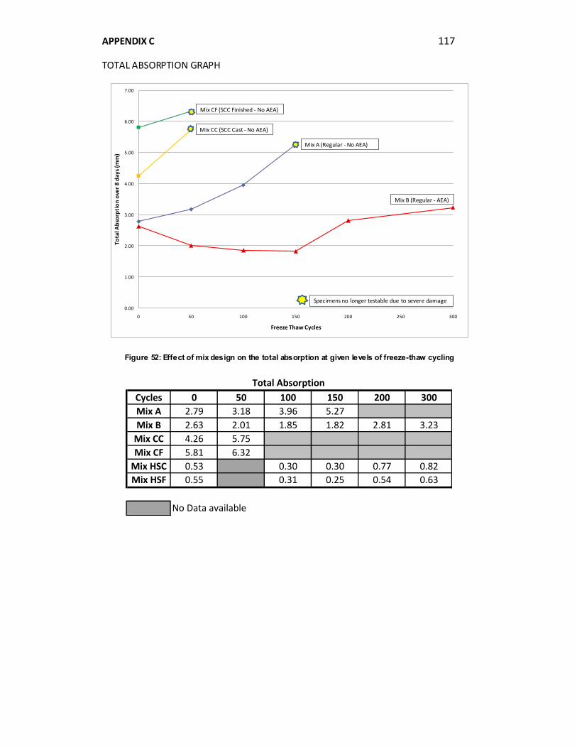
APPENDIX C 117
TOTAL ABSORPTION GRAPH
Figure 52: Effect of mix design on the total absorption at given levels of freeze-thaw cycling
0.00
1.00
2.00
3.00
4.00
5.00
6.00
7.00
0 50 100 150 200 250 300
Tota
l Ab
sorp
tio
n o
ver
8 d
ays
(mm
)
Freeze Thaw Cycles
Mix CF (SCC Finished - No AEA)
Mix CC (SCC Cast - No AEA)
Mix A (Regular - No AEA)
Mix B (Regular - AEA)
Specimens no longer testable due to severe damage
Cycles 0 50 100 150 200 300
Mix A 2.79 3.18 3.96 5.27
Mix B 2.63 2.01 1.85 1.82 2.81 3.23
Mix CC 4.26 5.75
Mix CF 5.81 6.32
Mix HSC 0.53 0.30 0.30 0.77 0.82
Mix HSF 0.55 0.31 0.25 0.54 0.63
No Data available
Total Absorption
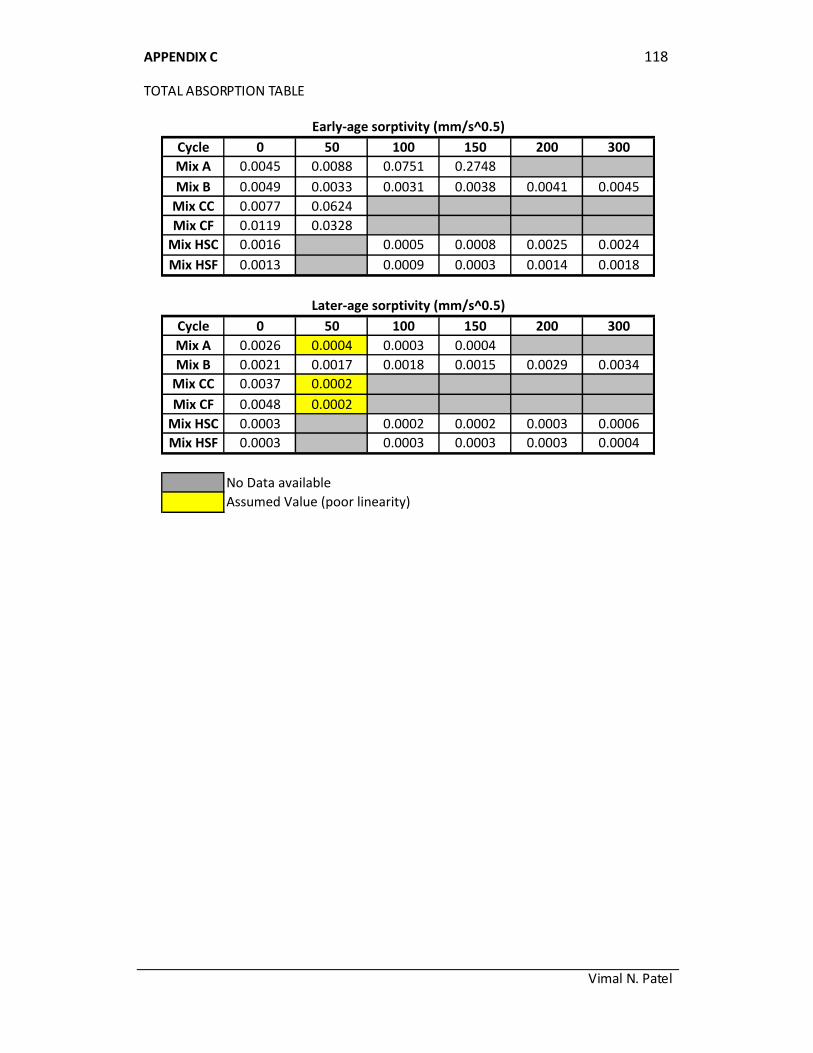
APPENDIX C 118
TOTAL ABSORPTION TABLE
Vimal N. Patel
Cycle 0 50 100 150 200 300
Mix A 0.0045 0.0088 0.0751 0.2748
Mix B 0.0049 0.0033 0.0031 0.0038 0.0041 0.0045
Mix CC 0.0077 0.0624
Mix CF 0.0119 0.0328
Mix HSC 0.0016 0.0005 0.0008 0.0025 0.0024
Mix HSF 0.0013 0.0009 0.0003 0.0014 0.0018
Cycle 0 50 100 150 200 300
Mix A 0.0026 0.0004 0.0003 0.0004
Mix B 0.0021 0.0017 0.0018 0.0015 0.0029 0.0034
Mix CC 0.0037 0.0002
Mix CF 0.0048 0.0002
Mix HSC 0.0003 0.0002 0.0002 0.0003 0.0006
Mix HSF 0.0003 0.0003 0.0003 0.0003 0.0004
No Data available
Assumed Value (poor linearity)
Early-age sorptivity (mm/s^0.5)
Later-age sorptivity (mm/s^0.5)
APPENDIX D 119
DATA FROM STATISTICAL ANALYSIS (EARLY-AGE SORPTIVITY)
Vimal N. Patel
α = 0.2
AW0 AT0 BW0 BT0 CCW0 CCT0 CFW0 CFT0
0.0038 0.0053 0.0048 0.0072 0.0082 0.0083 0.0115 0.0133
0.0052 0.0059 0.0042 0.0088 0.0072 0.0079 0.0121 0.0109
0.0046 0.0092 0.0056 0.0088 0.0076 0.0098 0.0121 0.0106
Mean = 0.004533333 0.0068 Mean = 0.004866667 0.008266667 Mean = 0.007666667 0.008666667 Mean = 0.0119 0.0116
variance = 4.93333E-07 0.00000441 variance = 4.93333E-07 8.53333E-07 variance = 2.53333E-07 1.00333E-06 variance = 0.00000012 0.00000219
Pooled Var 6.73333E-07 Pooled Var 6.28333E-07
F = 8.939189189 Tape Greater F = 1.72972973 Tape Greater F = 3.960526316 Tape Greater F = 18.25 Tape Greater
P fdsf 0.100611829 Reject Null P fdsf 0.366336634 Accept Null P fdsf 0.201591512 Accept Null P fdsf 0.051948052 Reject Null
F crit 4 Tape Greater F crit 4 NO F crit 4 NO F crit 4 Tape Greater
T stat 1.77297 Tape Greater T stat 5.07469 Tape Greater T stat 1.54508 Tape Greater T stat 0.34188 Wax Greater
P one-tail 0.10912 Reject Null P one-tail 0.00355 Reject Null P one-tail 0.09861 Reject Null P one-tail 0.38251 Accept Null
T crit one-tail 1.06066 Tape Greater T crit one-tail 0.94096 Tape Greater T crit one-tail 0.94096 Tape Greater T crit one-tail 1.06066 NO
P two-tail 0.21824 Accept Null P two-tail 0.00711 Reject Null P two-tail 0.19722 Reject Null P two-tail 0.76502 Accept Null
T crit two-tail 1.88562 NO T crit two-tail 1.53321 Tape Greater T crit two-tail 1.53321 Tape Greater T crit two-tail 1.88562 NO
AW50 AT50 BW50 BT50 CCW50 CCT50 CFW50 CFT50
0.008 0.0097 0.0031 0.0072 0.0629 0.0873 0.0414 0.0584
0.0095 0.0093 0.0036 0.0067 0.0608 0.0789 0.0748 0.0395
0.0126 0.0058 0.0031 0.0068 0.0634 0.0775 0.0241 0.0606
Mean = 0.010033333 0.008266667 Mean = 0.003266667 0.0069 Mean = 0.062366667 0.081233333 Mean = 0.046766667 0.052833333
variance = 5.50333E-06 4.60333E-06 variance = 8.33333E-08 7E-08 variance = 1.90333E-06 2.80933E-05 variance = 0.000664223 0.000134543
Pooled Var 5.05333E-06 Pooled Var 7.66667E-08
F = 1.1955105 Wax Greater F = 1.19047619 Wax Greater F = 14.76007005 Tape Greater F = 4.936872879 Wax Greater
P fdsf 0.455474934 Accept Null P fdsf 0.456521739 Accept Null P fdsf 0.063451495 Reject Null P fdsf 0.168438843 Reject Null
F crit 4 NO F crit 4 NO F crit 4 Tape Greater F crit 4 Wax Greater
T stat 0.96252 Wax Greater T stat 16.07117 Tape Greater T stat 5.96650 Tape Greater T stat 0.37179 Tape Greater
P one-tail 0.19515 Reject Null P one-tail 0.00004 Reject Null P one-tail 0.01348 Reject Null P one-tail 0.37287 Accept Null
T crit one-tail 0.94096 Wax Greater T crit one-tail 0.94096 Tape Greater T crit one-tail 1.06066 Tape Greater T crit one-tail 1.06066 NO
P two-tail 0.39029 Accept Null P two-tail 0.00009 Reject Null P two-tail 0.02696 Reject Null P two-tail 0.74574 Accept Null
T crit two-tail 1.53321 NO T crit two-tail 1.53321 Tape Greater T crit two-tail 1.88562 Tape Greater T crit two-tail 1.88562 NO
AW100 AT100 BW100 BT100
0.078 0.1271 0.0031 0.005
0.0729 0.1556 0.0033 0.0059
0.0743 0.1493 0.0028 0.0058
Mean = 0.075066667 0.144 Mean = 0.003066667 0.005566667
variance = 6.94333E-06 0.00022413 variance = 6.33333E-08 2.43333E-07
Pooled Var 1.53333E-07
F = 32.27988478 Tape Greater F = 3.842105263 Tape Greater
P fdsf 0.030048181 Reject Null P fdsf 0.206521739 Accept Null
F crit 4 Tape Greater F crit 4 NO
T stat 7.85444 Tape Greater T stat 7.81929 Tape Greater
P one-tail 0.00791 Reject Null P one-tail 0.00798 Reject Null
T crit one-tail 1.06066 Tape Greater T crit one-tail 1.06066 Tape Greater
P two-tail 0.01583 Reject Null P two-tail 0.01596 Reject Null
T crit two-tail 1.88562 Tape Greater T crit two-tail 1.88562 Tape Greater
F - TEST (0-6 Hours)
Null hypothesis that the variances and means are the same
F-TEST
T-TEST UNEQUAL VARIANCES
F-TEST F-TEST F-TEST
T-TEST EQUAL VARIANCES T-TEST EQUAL VARIANCES T-TEST UNEQUAL VARIANCES
T-TEST EQUAL VARIANCES T-TEST EQUAL VARIANCES T-TEST UNEQUAL VARIANCES T-TEST UNEQUAL VARIANCES
F-TEST F-TEST F-TEST F-TEST
F-TEST F-TEST
T-TEST UNEQUAL VARIANCES T-TEST UNEQUAL VARIANCES
APPENDIX D 120
DATA FROM STATISTICAL ANALYSIS (EARLY-AGE SORPTIVITY)
Vimal N. Patel
α = 0.2
AW150 AT150 BW150 BT150
0.2413 0.3398 0.004 0.0064
0.2872 0.2967 0.0034 0.0051
0.2958 0.0039 0.0074
Mean = 0.274766667 0.31825 Mean = 0.003766667 0.0063
variance = 0.000858503 0.000928805 variance = 1.03333E-07 0.00000133
Pooled Var 0.000893654
F = 1.081888636 Tape Greater F = 12.87096774 Tape Greater
P fdsf 0.480333089 Accept Null P fdsf 0.072093023 Reject Null
F crit 4 NO F crit 4 Tape Greater
T stat 1.78149 Tape Greater T stat 3.66505 Tape Greater
P one-tail 0.07471 Reject Null P one-tail 0.03352 Reject Null
T crit one-tail 0.94096 Tape Greater T crit one-tail 1.06066 Tape Greater
P two-tail 0.14942 Reject Null P two-tail 0.06705 Reject Null
T crit two-tail 1.53321 Tape Greater T crit two-tail 1.88562 Tape Greater
BW200 BT200
0.004 0.0078
0.0042 0.006
0.0032 0.0035
Mean = 0.0038 0.005766667
variance = 0.00000028 4.66333E-06
F = 16.6547619 Tape Greater
P fdsf 0.056641942 Reject Null
F crit 4 Tape Greater
T stat 0.00531 Tape Greater
P one-tail 0.49812 Accept Null
T crit one-tail 1.06066 NO
P two-tail 0.99624 Accept Null
T crit two-tail 1.88562 NO
BW300 BT300
0.0044 0.0089
0.0046 0.0066
0.0035 0.0095
Mean = 0.004166667 0.008333333
variance = 3.43333E-07 2.34333E-06
F = 6.825242718 Tape Greater
P fdsf 0.127791563 Reject Null
F crit 4 Tape Greater
T stat 0.09295 Tape Greater
P one-tail 0.46721 Accept Null
T crit one-tail 1.06066 NO
P two-tail 0.93441 Accept Null
T crit two-tail 1.88562 NO
F-TEST F-TEST
F-TEST
F-TEST
F - TEST (0-6 Hours) (cont.)
Null hypothesis that the variances and means are the same
T-TEST EQUAL VARIANCES T-TEST UNEQUAL VARIANCES
T-TEST UNEQUAL VARIANCES
T-TEST UNEQUAL VARIANCES
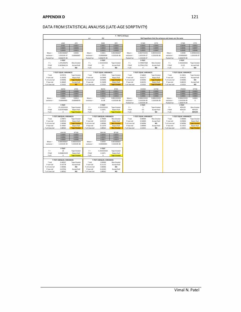
APPENDIX D 121
DATA FROM STATISTICAL ANALYSIS (LATE-AGE SORPTIVITY)
Vimal N. Patel
α = 0.2
AW0 AT0 BW0 BT0 CCW0 CCT0 CFW0 CFT0
0.002 0.0027 0.0021 0.0024 0.0042 0.0042 0.0049 0.0052
0.0025 0.0028 0.0019 0.0022 0.0035 0.0044 0.0046 0.0047
0.0026 0.0023 0.0023 0.0028 0.0035 0.0047 0.0049 0.0046
Mean = 0.002366667 0.0026 Mean = 0.0021 0.002466667 Mean = 0.003733333 0.004433333 Mean = 0.0048 0.004833333
variance = 1.03333E-07 0.00000007 variance = 0.00000004 9.33333E-08 variance = 1.63333E-07 6.33333E-08 variance = 0.00000003 1.03333E-07
Pooled Var 8.66667E-08 Pooled Var 6.66667E-08 Pooled Var 1.13333E-07 Pooled Var 6.66667E-08
F = 1.476190476 Wax Greater F = 2.333333333 Tape Greater F = 2.578947368 Wax Greater F = 3.444444444 Tape Greater
P fdsf 0.403846154 Accept Null P fdsf 0.3 Accept Null P fdsf 0.279411765 Accept Null P fdsf 0.225 Accept Null
F crit 4 NO F crit 4 NO F crit 4 NO F crit 4 NO
T stat 0.97073 Tape Greater T stat 1.73925 Tape Greater T stat 2.54662 Tape Greater T stat 0.15811 Tape Greater
P one-tail 0.19333 Reject Null P one-tail 0.07849 Reject Null P one-tail 0.03177 Reject Null P one-tail 0.44101 Accept Null
T crit one-tail 0.94096 Tape Greater T crit one-tail 0.94096 Tape Greater T crit one-tail 0.94096 Tape Greater T crit one-tail 0.94096 NO
P two-tail 0.38665 Accept Null P two-tail 0.15698 Reject Null P two-tail 0.06353 Reject Null P two-tail 0.88203 Accept Null
T crit two-tail 1.53321 NO T crit two-tail 1.53321 Tape Greater T crit two-tail 1.53321 Tape Greater T crit two-tail 1.53321 NO
AW50 AT50 BW50 BT50 CCW50 CCT50 CFW50 CFT50
0.0004 0.0009 0.0017 0.0011 0.0003 0.0002 0.0002 0.0003
0.0004 0.0007 0.0018 0.0015 0.0002 0.0003 0.0002 0.0003
0.0001 0.0023 0.0016 0.0014 0.0002 0.0002 0.0003 0.0003
Mean = 0.0003 0.0013 Mean = 0.0017 0.001333333 Mean = 0.000233333 0.000233333 Mean = 0.000233333 0.0003
variance = 0.00000003 0.00000076 variance = 1E-08 4.33333E-08 variance = 3.33333E-09 3.33333E-09 variance = 3.33333E-09 0
Pooled Var 3.33333E-09 Pooled Var 1.66667E-09
F = 25.33333333 Tape Greater F = 4.333333333 Tape Greater F = 1 Tape Greater F = #DIV/0! Wax Greater
P fdsf 0.037974684 Reject Null P fdsf 0.1875 Reject Null P fdsf 0.5 Accept Null P fdsf #DIV/0! #DIV/0!
F crit 4 Tape Greater F crit 4 Tape Greater F crit 4 NO F crit 4 #DIV/0!
T stat 1.94871 Tape Greater T stat 2.75000 Wax Greater T stat 0.00000 Wax Greater T stat 2.00000 Tape Greater
P one-tail 0.09533 Reject Null P one-tail 0.05535 Reject Null P one-tail 0.50000 Accept Null P one-tail 0.05806 Reject Null
T crit one-tail 1.06066 Tape Greater T crit one-tail 1.06066 Wax Greater T crit one-tail 0.94096 NO T crit one-tail 0.94096 Tape Greater
P two-tail 0.19067 Reject Null P two-tail 0.11070 Reject Null P two-tail 1.00000 Accept Null P two-tail 0.11612 Reject Null
T crit two-tail 1.88562 Tape Greater T crit two-tail 1.88562 Wax Greater T crit two-tail 1.53321 NO T crit two-tail 1.53321 Tape Greater
AW100 AT100 BW100 BT100
0.0003 0.0002 0.0018 0.0015
0.0002 0.0002 0.0019 0.0016
0.0003 0.0006 0.0017 0.0019
Mean = 0.000266667 0.000333333 Mean = 0.0018 0.001666667
variance = 3.33333E-09 5.33333E-08 variance = 0.00000001 4.33333E-08
F = 16 Tape Greater F = 4.333333333 Tape Greater
P fdsf 0.058823529 Reject Null P fdsf 0.1875 Reject Null
F crit 4 Tape Greater F crit 4 Tape Greater
T stat 0.48507 Tape Greater T stat 1.00000 Wax Greater
P one-tail 0.33778 Accept Null P one-tail 0.21132 Accept Null
T crit one-tail 1.06066 NO T crit one-tail 1.06066 NO
P two-tail 0.67556 Accept Null P two-tail 0.42265 Accept Null
T crit two-tail 1.88562 NO T crit two-tail 1.88562 NO
F - TEST (1-8 Days)
Null hypothesis that the variances and means are the same
F-TEST F-TEST F-TEST F-TEST
F-TEST F-TEST F-TEST F-TEST
T-TEST EQUAL VARIANCES T-TEST EQUAL VARIANCES
F-TEST F-TEST
T-TEST UNEQUAL VARIANCES T-TEST UNEQUAL VARIANCES
T-TEST EQUAL VARIANCES T-TEST EQUAL VARIANCES
T-TEST EQUAL VARIANCEST-TEST EQUAL VARIANCEST-TEST UNEQUAL VARIANCES T-TEST UNEQUAL VARIANCES
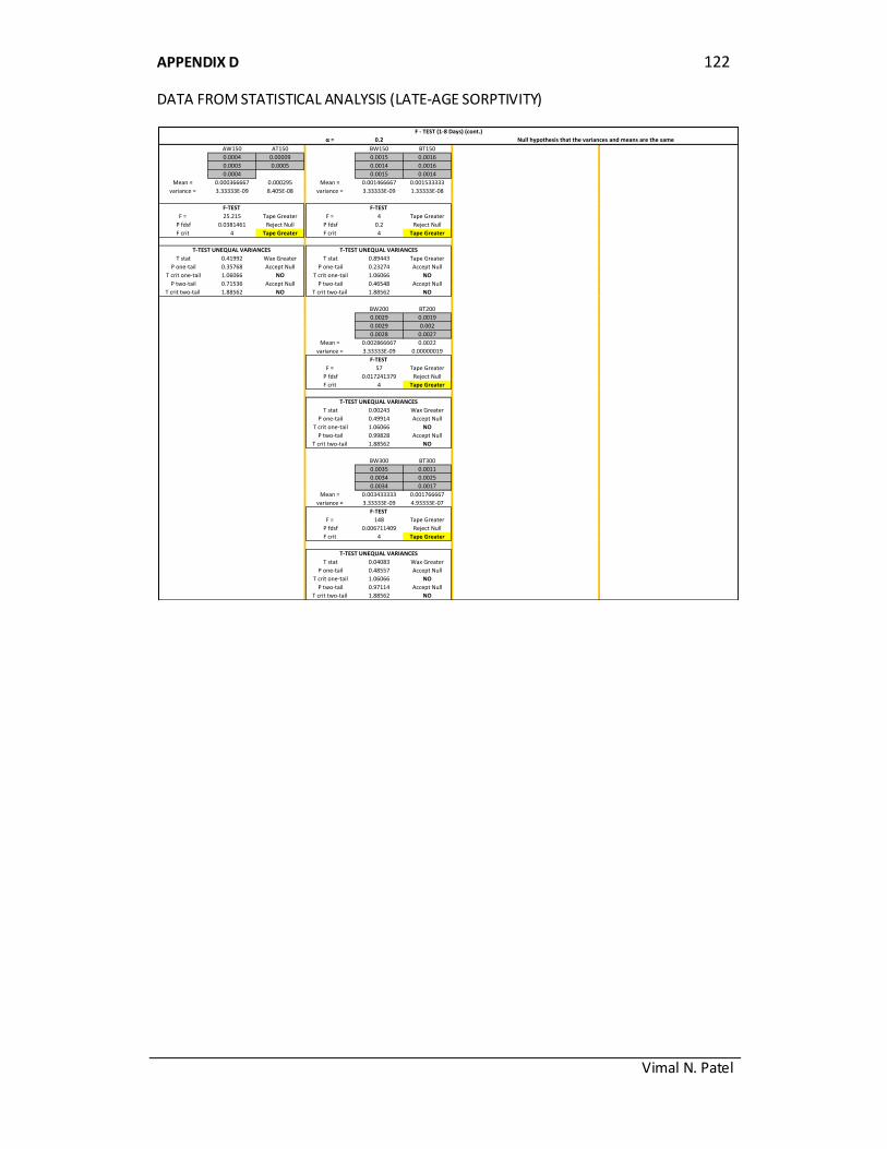
APPENDIX D 122
DATA FROM STATISTICAL ANALYSIS (LATE-AGE SORPTIVITY)
Vimal N. Patel
α = 0.2
AW150 AT150 BW150 BT150
0.0004 0.00009 0.0015 0.0016
0.0003 0.0005 0.0014 0.0016
0.0004 0.0015 0.0014
Mean = 0.000366667 0.000295 Mean = 0.001466667 0.001533333
variance = 3.33333E-09 8.405E-08 variance = 3.33333E-09 1.33333E-08
F = 25.215 Tape Greater F = 4 Tape Greater
P fdsf 0.0381461 Reject Null P fdsf 0.2 Reject Null
F crit 4 Tape Greater F crit 4 Tape Greater
T stat 0.41992 Wax Greater T stat 0.89443 Tape Greater
P one-tail 0.35768 Accept Null P one-tail 0.23274 Accept Null
T crit one-tail 1.06066 NO T crit one-tail 1.06066 NO
P two-tail 0.71536 Accept Null P two-tail 0.46548 Accept Null
T crit two-tail 1.88562 NO T crit two-tail 1.88562 NO
BW200 BT200
0.0029 0.0019
0.0029 0.002
0.0028 0.0027
Mean = 0.002866667 0.0022
variance = 3.33333E-09 0.00000019
F = 57 Tape Greater
P fdsf 0.017241379 Reject Null
F crit 4 Tape Greater
T stat 0.00243 Wax Greater
P one-tail 0.49914 Accept Null
T crit one-tail 1.06066 NO
P two-tail 0.99828 Accept Null
T crit two-tail 1.88562 NO
BW300 BT300
0.0035 0.0011
0.0034 0.0025
0.0034 0.0017
Mean = 0.003433333 0.001766667
variance = 3.33333E-09 4.93333E-07
F = 148 Tape Greater
P fdsf 0.006711409 Reject Null
F crit 4 Tape Greater
T stat 0.04083 Wax Greater
P one-tail 0.48557 Accept Null
T crit one-tail 1.06066 NO
P two-tail 0.97114 Accept Null
T crit two-tail 1.88562 NO
F-TEST F-TEST
F-TEST
F-TEST
T-TEST UNEQUAL VARIANCES T-TEST UNEQUAL VARIANCES
F - TEST (1-8 Days) (cont.)
Null hypothesis that the variances and means are the same
T-TEST UNEQUAL VARIANCES
T-TEST UNEQUAL VARIANCES