sorting and algorithm analysis
TRANSCRIPT
Sorting and Algorithm Analysis
Computer Science E-119Harvard Extension School
Fall 2012
David G. Sullivan, Ph.D.
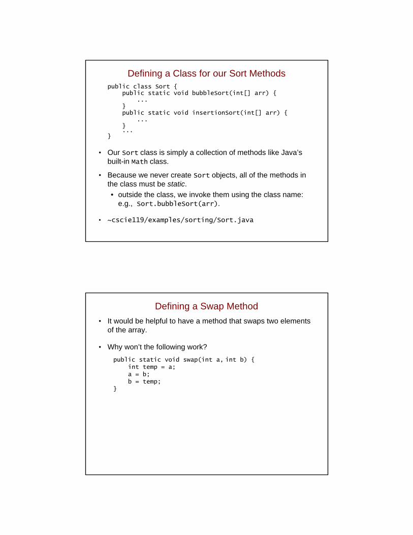
Sorting an Array of Integers
• Ground rules:• sort the values in increasing order• sort “in place,” using only a small amount of additional storage
• Terminology:• position: one of the memory locations in the array• element: one of the data items stored in the array• element i: the element at position i
• Goal: minimize the number of comparisons C and the number of moves M needed to sort the array.
• move = copying an element from one position to anotherexample: arr[3] = arr[5];
15 7 36
0 1 2
arr 40 12
n-2 n-1…
Defining a Class for our Sort Methodspublic class Sort {
public static void bubbleSort(int[] arr) {...
}public static void insertionSort(int[] arr) {
...}...
}
• Our Sort class is simply a collection of methods like Java’s built-in Math class.
• Because we never create Sort objects, all of the methods in the class must be static.
• outside the class, we invoke them using the class name: e.g., Sort.bubbleSort(arr).
• ~cscie119/examples/sorting/Sort.java
Defining a Swap Method
• It would be helpful to have a method that swaps two elements of the array.
• Why won’t the following work?
public static void swap(int a, int b) {int temp = a;a = b;b = temp;
}
public static void swap(int a, int b) {int temp = a;a = b;b = temp;
}
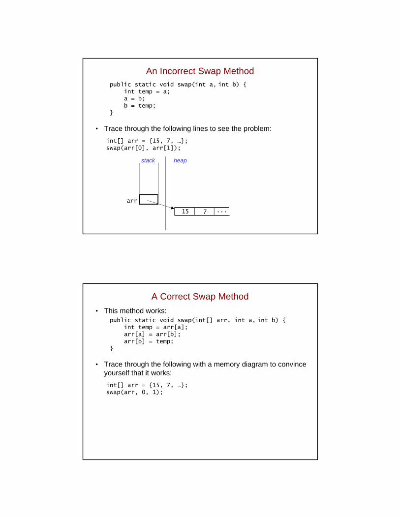
• Trace through the following lines to see the problem:
int[] arr = {15, 7, …};swap(arr[0], arr[1]);
stack heap
...
arr
An Incorrect Swap Method
15 7
A Correct Swap Method
• This method works:public static void swap(int[] arr, int a, int b) {
int temp = arr[a];arr[a] = arr[b];arr[b] = temp;
}
• Trace through the following with a memory diagram to convince yourself that it works:
int[] arr = {15, 7, …};swap(arr, 0, 1);
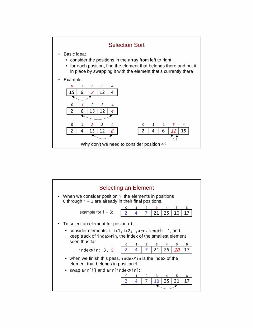
Selection Sort
• Basic idea:• consider the positions in the array from left to right• for each position, find the element that belongs there and put it
in place by swapping it with the element that’s currently there
• Example:
15 6 2 12 4
0 1 2 3 4
2
0
2 6 15 12 4
0 1 2 3 4
4
1
2 4 15 12 6
0 1 2 3 4
6
2
2 4 6 12 15
0 1 2 3 4
12
3
Why don’t we need to consider position 4?
Selecting an Element
• When we consider position i, the elements in positions 0 through i – 1 are already in their final positions.
example for i = 3:
• To select an element for position i:
• consider elements i, i+1,i+2,…,arr.length – 1, andkeep track of indexMin, the index of the smallest element seen thus far
• when we finish this pass, indexMin is the index of the element that belongs in position i.
• swap arr[i] and arr[indexMin]:
2 4 7 21 25 10 17
0 1 2 3 4 5 6
indexMin: 3 2 4 7 21 25 10 17
0 1 2 3 4 5 6
2 4 7 21 25 10 17
0 1 2 3 4 5 6
10 21
, 5 1010
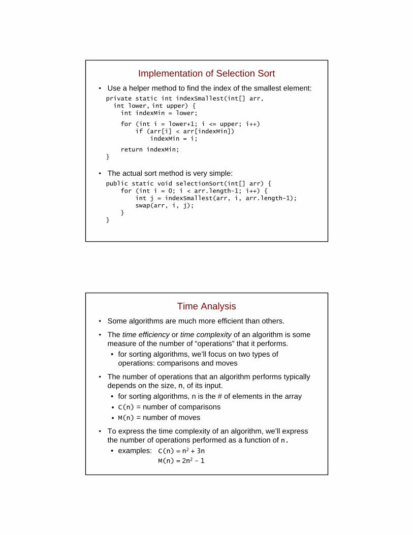
Implementation of Selection Sort
• Use a helper method to find the index of the smallest element:private static int indexSmallest(int[] arr,
int lower, int upper) {int indexMin = lower;
for (int i = lower+1; i <= upper; i++)if (arr[i] < arr[indexMin])
indexMin = i;
return indexMin;}
• The actual sort method is very simple:public static void selectionSort(int[] arr) {
for (int i = 0; i < arr.length-1; i++) {int j = indexSmallest(arr, i, arr.length-1);swap(arr, i, j);
}}
Time Analysis
• Some algorithms are much more efficient than others.
• The time efficiency or time complexity of an algorithm is some measure of the number of “operations” that it performs.
• for sorting algorithms, we’ll focus on two types of operations: comparisons and moves
• The number of operations that an algorithm performs typically depends on the size, n, of its input.
• for sorting algorithms, n is the # of elements in the array
• C(n) = number of comparisons
• M(n) = number of moves
• To express the time complexity of an algorithm, we’ll express the number of operations performed as a function of n.
• examples: C(n) = n2 + 3n
M(n) = 2n2 - 1
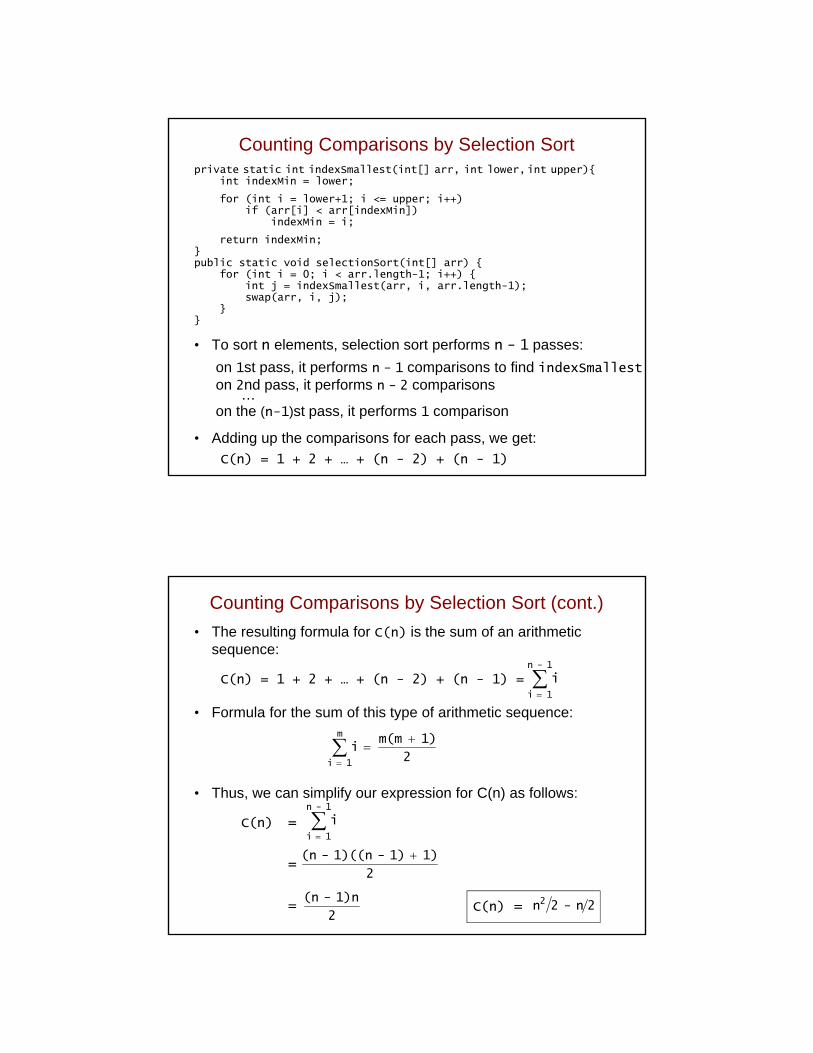
Counting Comparisons by Selection Sortprivate static int indexSmallest(int[] arr, int lower,int upper){
int indexMin = lower;
for (int i = lower+1; i <= upper; i++)if (arr[i] < arr[indexMin])
indexMin = i;
return indexMin;}public static void selectionSort(int[] arr) {
for (int i = 0; i < arr.length-1; i++) {int j = indexSmallest(arr, i, arr.length-1);swap(arr, i, j);
}}
• To sort n elements, selection sort performs n - 1 passes:
on 1st pass, it performs n - 1 comparisons to find indexSmalleston 2nd pass, it performs n - 2 comparisons
…on the (n-1)st pass, it performs 1 comparison
• Adding up the comparisons for each pass, we get:
C(n) = 1 + 2 + … + (n - 2) + (n - 1)
Counting Comparisons by Selection Sort (cont.)
• The resulting formula for C(n) is the sum of an arithmetic sequence:
C(n) = 1 + 2 + … + (n - 2) + (n - 1) =
• Formula for the sum of this type of arithmetic sequence:
• Thus, we can simplify our expression for C(n) as follows:
C(n) =
=
=
1 - n
1 i
i
2
1)m(m i
m
1 i
1 - n
1 i
i
2
1)1)-1)((n-(n
2
1)n-(n 2n- 2n2C(n) =
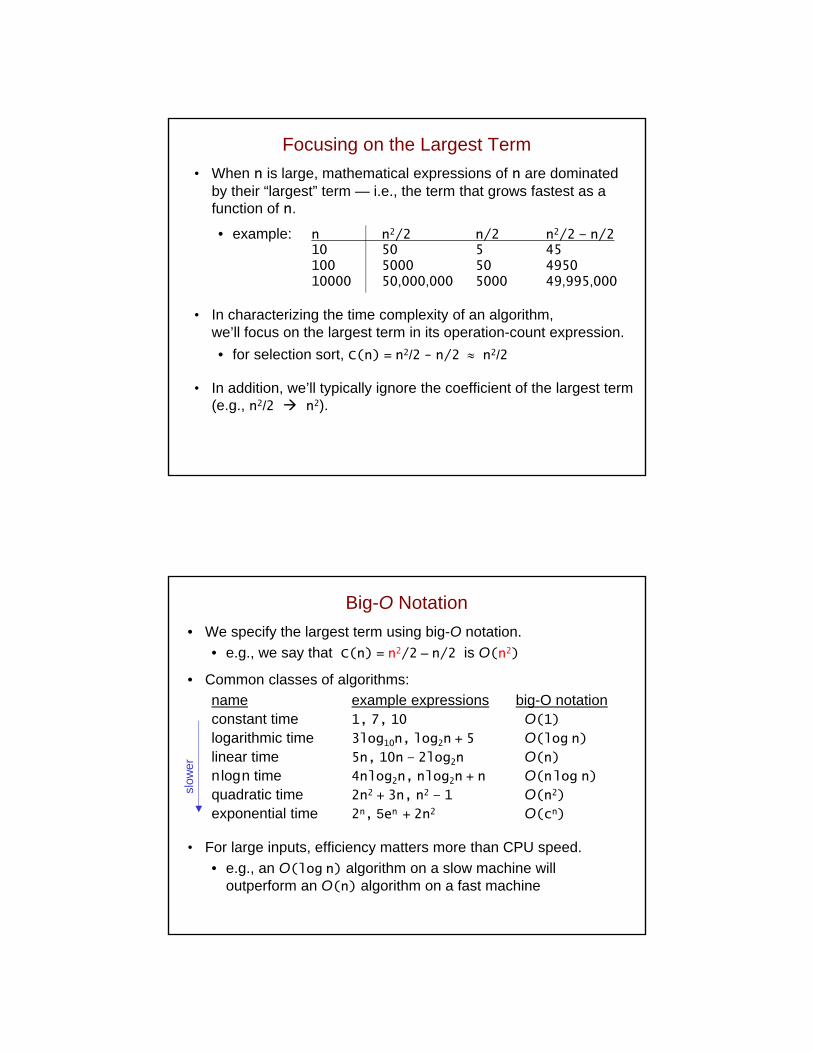
Focusing on the Largest Term
• When n is large, mathematical expressions of n are dominated by their “largest” term — i.e., the term that grows fastest as a function of n.
• example: n n2/2 n/2 n2/2 – n/210 50 5 45100 5000 50 495010000 50,000,000 5000 49,995,000
• In characterizing the time complexity of an algorithm, we’ll focus on the largest term in its operation-count expression.
• for selection sort, C(n) = n2/2 - n/2 n2/2
• In addition, we’ll typically ignore the coefficient of the largest term (e.g., n2/2 n2).
Big-O Notation
• We specify the largest term using big-O notation.
• e.g., we say that C(n) = n2/2 – n/2 is O(n2)
• Common classes of algorithms:
name example expressions big-O notationconstant time 1, 7, 10 O(1)
logarithmic time 3log10n, log2n + 5 O(log n)
linear time 5n, 10n – 2log2n O(n)
nlogn time 4nlog2n, nlog2n + n O(nlog n)
quadratic time 2n2 + 3n, n2 – 1 O(n2)
exponential time 2n, 5en + 2n2 O(cn)
• For large inputs, efficiency matters more than CPU speed.
• e.g., an O(log n) algorithm on a slow machine will outperform an O(n) algorithm on a fast machine
slow
er
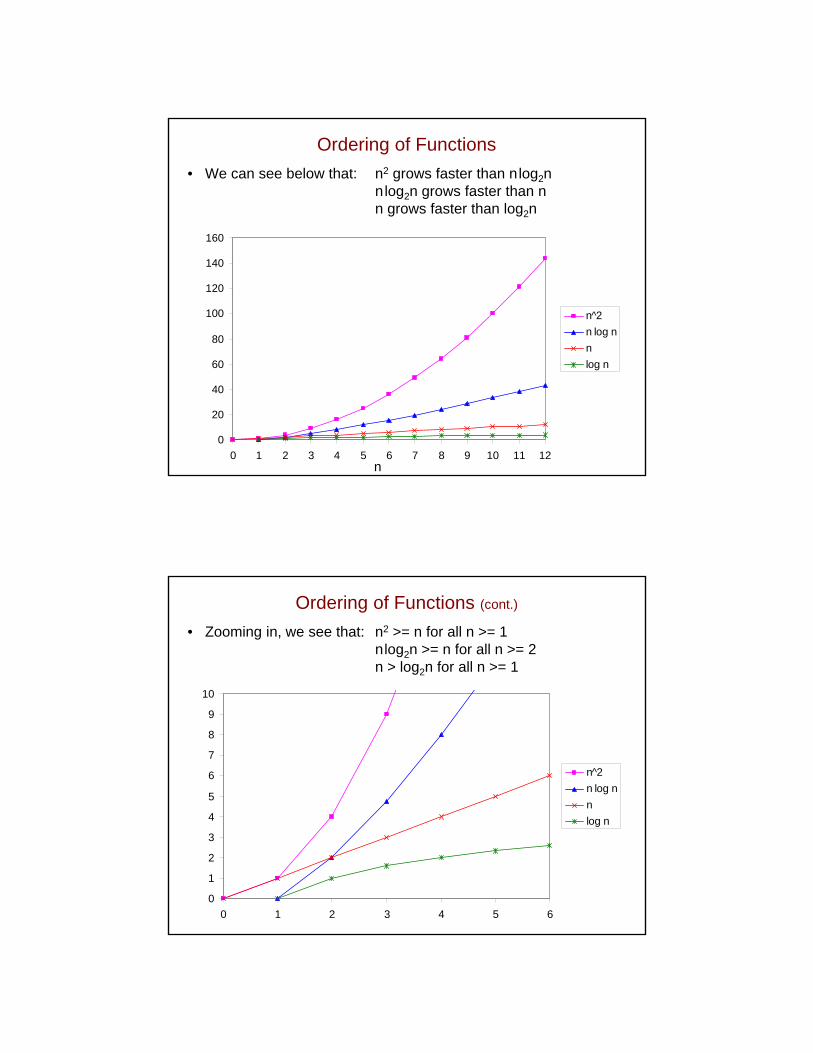
Ordering of Functions
• We can see below that: n2 grows faster than nlog2nnlog2n grows faster than nn grows faster than log2n
0
20
40
60
80
100
120
140
160
0 1 2 3 4 5 6 7 8 9 10 11 12
n^2
n log n
n
log n
n
Ordering of Functions (cont.)
• Zooming in, we see that: n2 >= n for all n >= 1nlog2n >= n for all n >= 2n > log2n for all n >= 1
0
1
2
3
4
5
6
7
8
9
10
0 1 2 3 4 5 6
n^2
n log n
n
log n
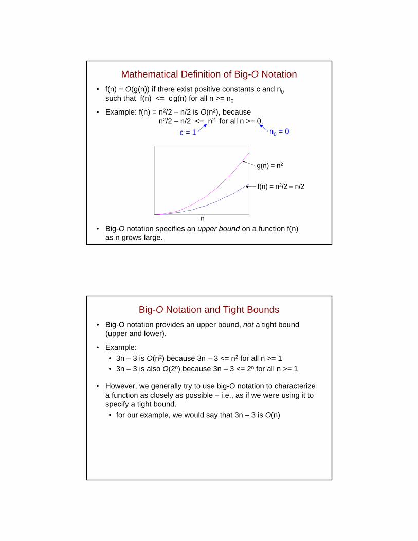
Mathematical Definition of Big-O Notation
• f(n) = O(g(n)) if there exist positive constants c and n0
such that f(n) <= cg(n) for all n >= n0
• Example: f(n) = n2/2 – n/2 is O(n2), becausen2/2 – n/2 <= n2 for all n >= 0.
• Big-O notation specifies an upper bound on a function f(n) as n grows large.
n
f(n) = n2/2 – n/2
g(n) = n2
c = 1 n0 = 0
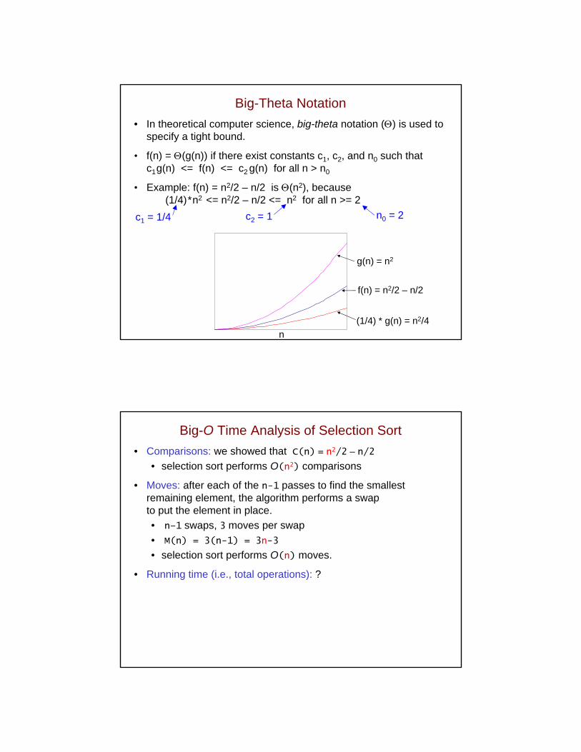
Big-O Notation and Tight Bounds
• Big-O notation provides an upper bound, not a tight bound (upper and lower).
• Example:
• 3n – 3 is O(n2) because 3n – 3 <= n2 for all n >= 1
• 3n – 3 is also O(2n) because 3n – 3 <= 2n for all n >= 1
• However, we generally try to use big-O notation to characterize a function as closely as possible – i.e., as if we were using it to specify a tight bound.
• for our example, we would say that 3n – 3 is O(n)
Big-Theta Notation
• In theoretical computer science, big-theta notation () is used to specify a tight bound.
• f(n) = (g(n)) if there exist constants c1, c2, and n0 such thatc1g(n) <= f(n) <= c2 g(n) for all n > n0
• Example: f(n) = n2/2 – n/2 is (n2), because(1/4)*n2 <= n2/2 – n/2 <= n2 for all n >= 2
n
(1/4) * g(n) = n2/4
f(n) = n2/2 – n/2
g(n) = n2
c1 = 1/4 n0 = 2c2 = 1
Big-O Time Analysis of Selection Sort
• Comparisons: we showed that C(n) = n2/2 – n/2
• selection sort performs O(n2) comparisons
• Moves: after each of the n-1 passes to find the smallest remaining element, the algorithm performs a swapto put the element in place.
• n–1 swaps, 3 moves per swap
• M(n) = 3(n-1) = 3n-3
• selection sort performs O(n) moves.
• Running time (i.e., total operations): ?
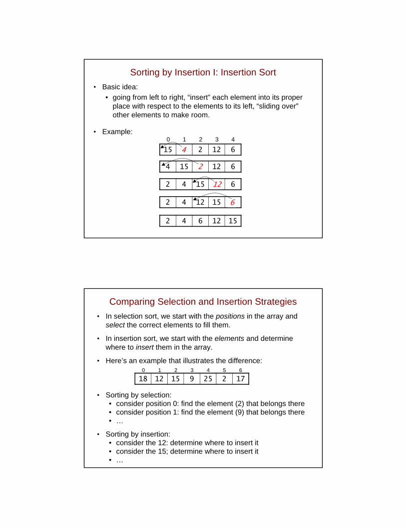
Sorting by Insertion I: Insertion Sort
• Basic idea:
• going from left to right, “insert” each element into its proper place with respect to the elements to its left, “sliding over” other elements to make room.
• Example:
15 4 2 12 6
0 1 2 3 4
4 15 2 12 6
2 4 15 12 6
2 4 12 15 6
2 4 6 12 15
4
2
12
6
Comparing Selection and Insertion Strategies
• In selection sort, we start with the positions in the array and select the correct elements to fill them.
• In insertion sort, we start with the elements and determine where to insert them in the array.
• Here’s an example that illustrates the difference:
• Sorting by selection:• consider position 0: find the element (2) that belongs there• consider position 1: find the element (9) that belongs there• …
• Sorting by insertion:• consider the 12: determine where to insert it• consider the 15; determine where to insert it• …
18 12 15 9 25 2 17
0 1 2 3 4 5 6
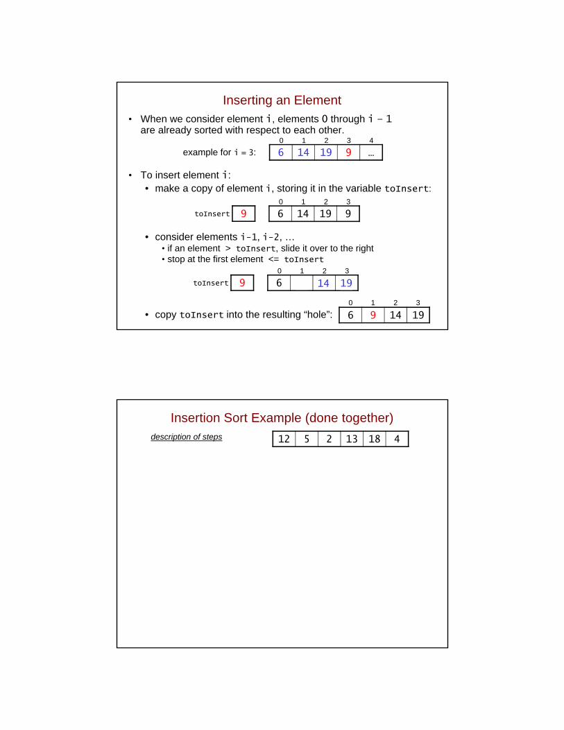
Inserting an Element• When we consider element i, elements 0 through i – 1
are already sorted with respect to each other.
example for i = 3:
• To insert element i:• make a copy of element i, storing it in the variable toInsert:
• consider elements i-1, i-2, …• if an element > toInsert, slide it over to the right • stop at the first element <= toInsert
• copy toInsert into the resulting “hole”:
6 14 19 9 …
0 1 2 3 4
6 14 19 9
0 1 2 3
6 9 14 19
0 1 2 3
9toInsert
6 14 19 9
0 1 2 3
9toInsert 1914
Insertion Sort Example (done together)description of steps 12 5 2 13 18 4
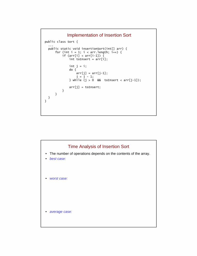
Implementation of Insertion Sortpublic class Sort {
...public static void insertionSort(int[] arr) {
for (int i = 1; i < arr.length; i++) {if (arr[i] < arr[i-1]) {
int toInsert = arr[i];
int j = i;do {
arr[j] = arr[j-1];j = j - 1;
} while (j > 0 && toInsert < arr[j-1]);
arr[j] = toInsert;}
}}
}
Time Analysis of Insertion Sort
• The number of operations depends on the contents of the array.
• best case: array is sortedthus, we never execute the do-while loopeach element is only compared to the element to its leftC(n) = n – 1 = O(n), M(n) = 0, running time = O(n)
• worst case: array is in reverse ordereach element is compared to all of the elements to its left:
arr[1] is compared to 1 element (arr[0])arr[2] is compared to 2 elements (arr[0] and arr[1])…arr[n-1] is compared to n-1 elements
C(n) = 1 + 2 + … + (n – 1) = O(n2) as seen in selection sortsimilarly, M(n) = O(n2), running time = O(n2)
• average case:
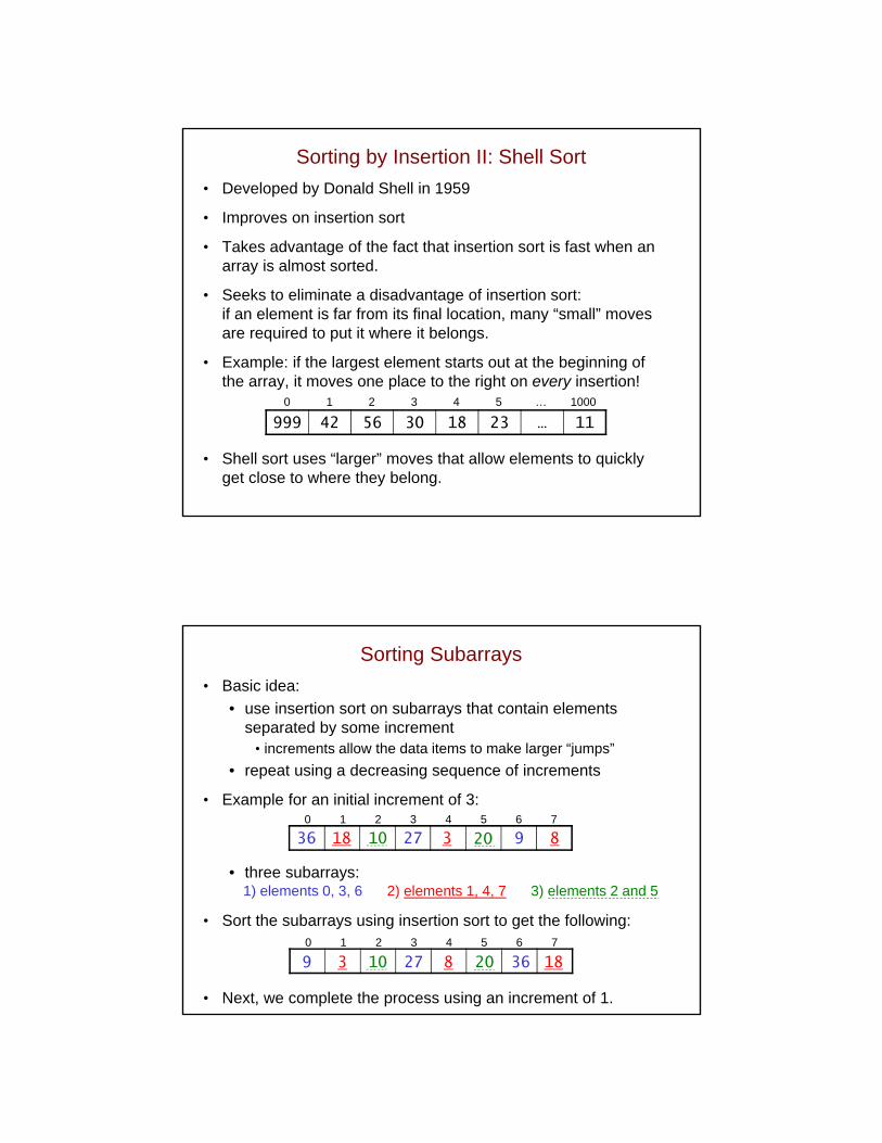
Sorting by Insertion II: Shell Sort
• Developed by Donald Shell in 1959
• Improves on insertion sort
• Takes advantage of the fact that insertion sort is fast when an array is almost sorted.
• Seeks to eliminate a disadvantage of insertion sort: if an element is far from its final location, many “small” moves are required to put it where it belongs.
• Example: if the largest element starts out at the beginning of the array, it moves one place to the right on every insertion!
• Shell sort uses “larger” moves that allow elements to quickly get close to where they belong.
999 42 56 30 18 23 … 11
0 1 2 3 4 5 … 1000
3) elements 2 and 5
Sorting Subarrays
• Basic idea:
• use insertion sort on subarrays that contain elements separated by some increment
• increments allow the data items to make larger “jumps”
• repeat using a decreasing sequence of increments
• Example for an initial increment of 3:
• three subarrays:
• Sort the subarrays using insertion sort to get the following:
• Next, we complete the process using an increment of 1.
36 18 10 27 3 20 9 8
0 1 2 3 4 5 6 7
6 23 14 27 18 20 9 3
0 1 2 3 4 5 6 7
9 3 10 27 8 20 36 18
36 18 27 3 9 8
1) elements 0, 3, 6 2) elements 1, 4, 7
10 20
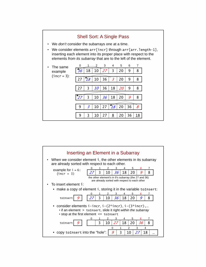
Shell Sort: A Single Pass
• We don’t consider the subarrays one at a time.
• We consider elements arr[incr] through arr[arr.length-1], inserting each element into its proper place with respect to the elements from its subarray that are to the left of the element.
• The sameexample(incr = 3):
36 18 10 27 3 20 9 8
0 1 2 3 4 5 6 7
27 18 10 36 3 20 9 8
27 3 10 36 18 20 9 8
27 3 10 36 18 20 9 8
9 3 10 27 18 20 36 8
20
9
8
9 3 10 27 8 20 36 18
36
18
10
27 36
3 18
27
3
• When we consider element i, the other elements in its subarrayare already sorted with respect to each other.
example for i = 6:(incr = 3)
the other element’s in 9’s subarray (the 27 and 36) are already sorted with respect to each other
• To insert element i:• make a copy of element i, storing it in the variable toInsert:
• consider elements i-incr, i-(2*incr), i-(3*incr),…• if an element > toInsert, slide it right within the subarray• stop at the first element <= toInsert
• copy toInsert into the “hole”:
27 3 10 36 18 20 9 8
0 1 2 3 4 5 6 7
9 3 10 27 18 …
0 1 2 3 4
9toInsert
27 3 10 36 18 20 9 8
0 1 2 3 4 5 6 7
9toInsert 36
Inserting an Element in a Subarray
27 3 10 36 18 20 9 8
0 1 2 3 4 5 6 7
27
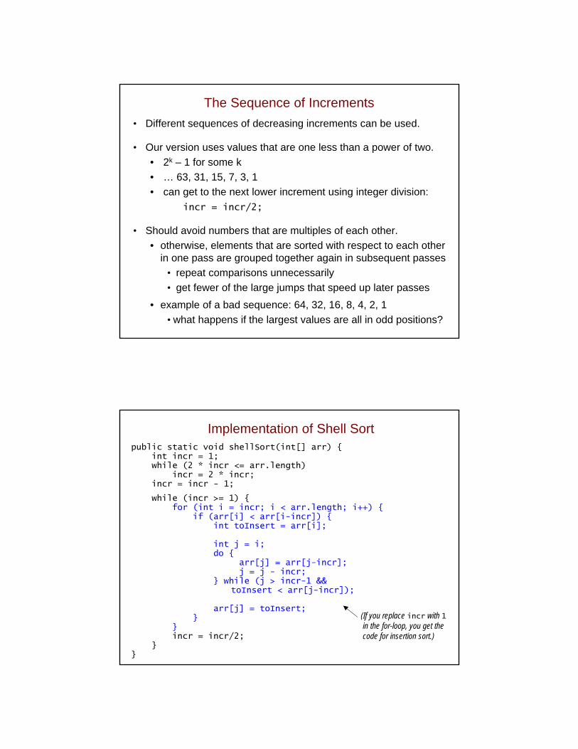
The Sequence of Increments
• Different sequences of decreasing increments can be used.
• Our version uses values that are one less than a power of two.
• 2k – 1 for some k
• … 63, 31, 15, 7, 3, 1
• can get to the next lower increment using integer division:
incr = incr/2;
• Should avoid numbers that are multiples of each other.
• otherwise, elements that are sorted with respect to each other in one pass are grouped together again in subsequent passes
• repeat comparisons unnecessarily
• get fewer of the large jumps that speed up later passes
• example of a bad sequence: 64, 32, 16, 8, 4, 2, 1
• what happens if the largest values are all in odd positions?
Implementation of Shell Sortpublic static void shellSort(int[] arr) {
int incr = 1;while (2 * incr <= arr.length)
incr = 2 * incr;incr = incr - 1;
while (incr >= 1) {for (int i = incr; i < arr.length; i++) {
if (arr[i] < arr[i-incr]) {int toInsert = arr[i];
int j = i;do {
arr[j] = arr[j-incr];j = j - incr;
} while (j > incr-1 && toInsert < arr[j-incr]);
arr[j] = toInsert;}
}incr = incr/2;
}}
(If you replace incr with 1in the for-loop, you get thecode for insertion sort.)
Time Analysis of Shell Sort
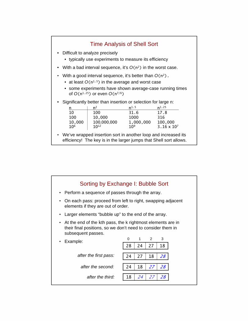
• Difficult to analyze precisely
• typically use experiments to measure its efficiency
• With a bad interval sequence, it’s O(n2) in the worst case.
• With a good interval sequence, it’s better than O(n2).
• at least O(n1.5) in the average and worst case
• some experiments have shown average-case running times of O(n1.25) or even O(n7/6)
• Significantly better than insertion or selection for large n:n n2 n1.5 n1.25
10 100 31.6 17.8100 10,000 1000 31610,000 100,000,000 1,000,000 100,000106 1012 109 3.16 x 10⁷
• We’ve wrapped insertion sort in another loop and increased its efficiency! The key is in the larger jumps that Shell sort allows.
Sorting by Exchange I: Bubble Sort
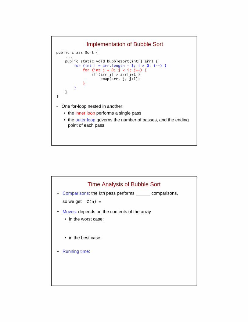
• Perform a sequence of passes through the array.
• On each pass: proceed from left to right, swapping adjacent elements if they are out of order.
• Larger elements “bubble up” to the end of the array.
• At the end of the kth pass, the k rightmost elements are in their final positions, so we don’t need to consider them in subsequent passes.
• Example:
after the first pass:
after the second:
after the third:
28 24 27 18
0 1 2 3
24 27 18 28
24 18 27 28
18 24 27 28
Implementation of Bubble Sortpublic class Sort {
...public static void bubbleSort(int[] arr) {
for (int i = arr.length – 1; i > 0; i--) {for (int j = 0; j < i; j++) {
if (arr[j] > arr[j+1])swap(arr, j, j+1);
}}
}}
• One for-loop nested in another:
• the inner loop performs a single pass
• the outer loop governs the number of passes, and the ending point of each pass
Time Analysis of Bubble Sort
• Comparisons: the kth pass performs comparisons,
so we get C(n) =
• Moves: depends on the contents of the array
• in the worst case:
• in the best case:
• Running time:
Sorting by Exchange II: Quicksort
• Like bubble sort, quicksort uses an approach based on exchanging out-of-order elements, but it’s more efficient.
• A recursive, divide-and-conquer algorithm:
• divide: rearrange the elements so that we end up with two subarrays that meet the following criterion:
each element in the left array <= each element in the right array
example:
• conquer: apply quicksort recursively to the subarrays, stopping when a subarray has a single element
• combine: nothing needs to be done, because of the criterionused in forming the subarrays
12 8 14 4 6 13 6 8 4 14 12 13
Partitioning an Array Using a Pivot
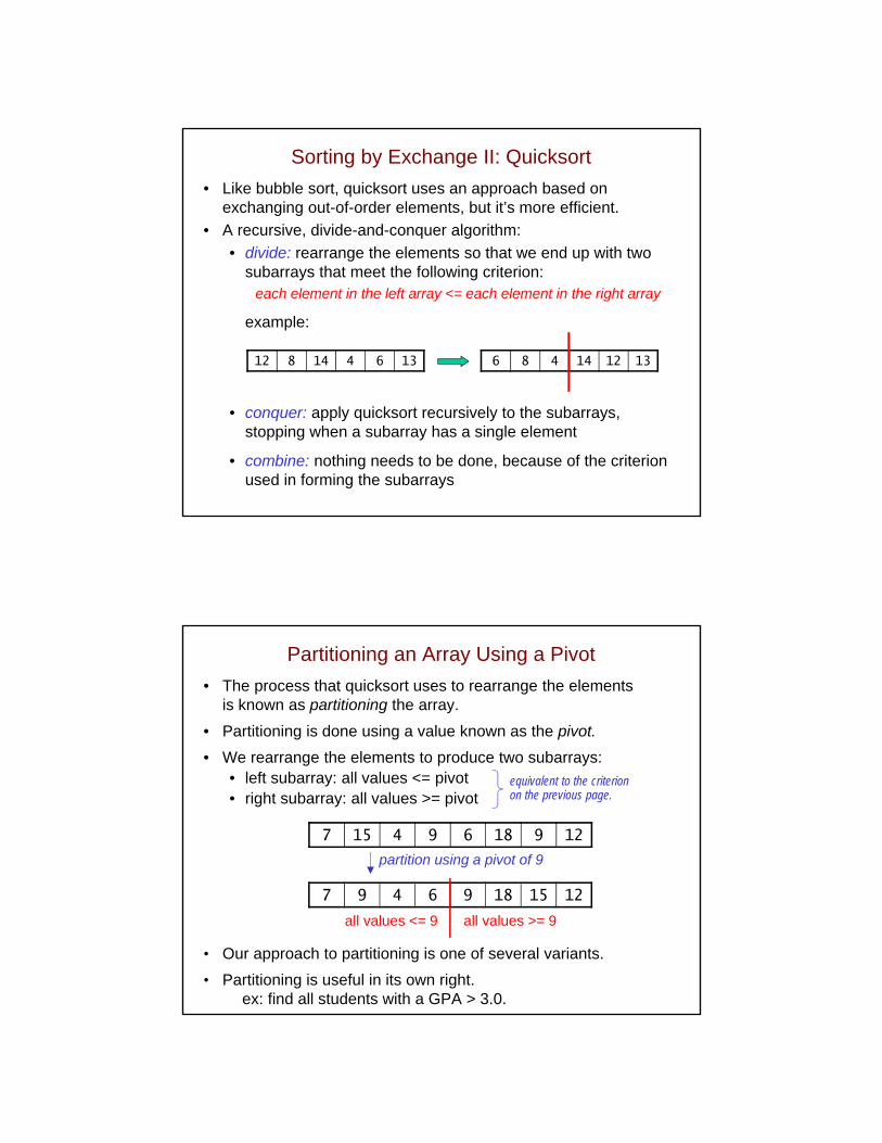
• The process that quicksort uses to rearrange the elements is known as partitioning the array.
• Partitioning is done using a value known as the pivot.
• We rearrange the elements to produce two subarrays:• left subarray: all values <= pivot• right subarray: all values >= pivot
• Our approach to partitioning is one of several variants.
• Partitioning is useful in its own right. ex: find all students with a GPA > 3.0.
7 15 4 9 6 18 9 12
7 9 4 6 9 18 15 12
all values <= 9 all values >= 9
partition using a pivot of 9
equivalent to the criterionon the previous page.
Possible Pivot Values
• First element or last element
• risky, can lead to terrible worst-case behavior
• especially poor if the array is almost sorted
• Middle element (what we will use)
• Randomly chosen element
• Median of three elements
• left, center, and right elements
• three randomly selected elements
• taking the median of three decreases the probability of getting a poor pivot
4 8 14 12 6 18 4 8 14 12 6 18
pivot = 18
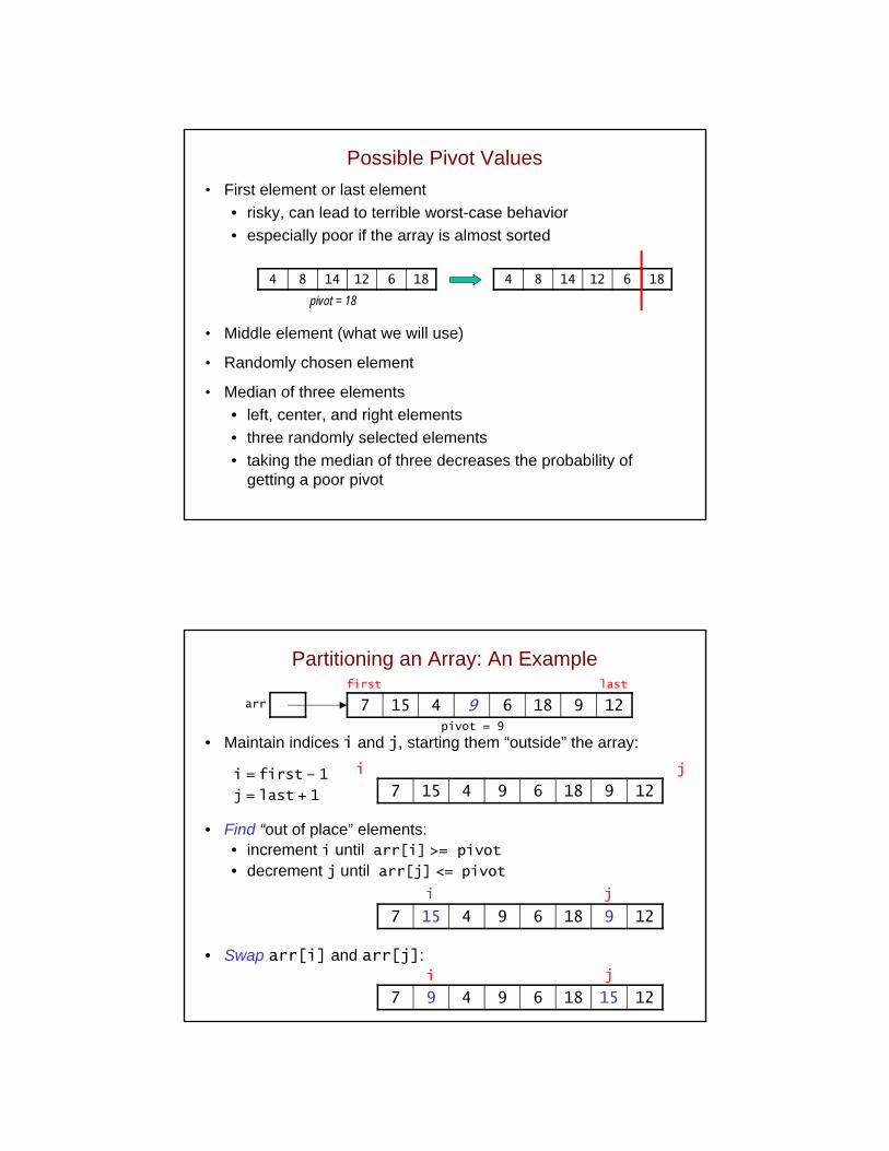
Partitioning an Array: An Example
• Maintain indices i and j, starting them “outside” the array:
• Find “out of place” elements: • increment i until arr[i] >= pivot
• decrement j until arr[j] <= pivot
• Swap arr[i] and arr[j]:
7 15 4 9 6 18 9 12
7 15 4 9 6 18 9 12
7 9 4 9 6 18 15 12
i j
i j
i j
i = first – 1
j = last + 1
7 15 4 9 6 18 9 12arr
pivot = 9
first last
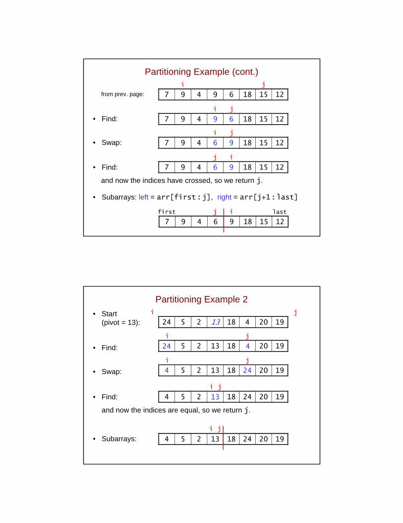
Partitioning Example (cont.)
from prev. page:
• Find:
• Swap:
• Find:
and now the indices have crossed, so we return j.
• Subarrays: left = arr[first:j], right = arr[j+1:last]
7 9 4 9 6 18 15 12
7 9 4 9 6 18 15 12
7 9 4 6 9 18 15 12
i j
i j
7 9 4 6 9 18 15 12
i j
7 9 4 6 9 18 15 12
j i
j ifirst last
Partitioning Example 2
• Start(pivot = 13):
• Find:
• Swap:
• Find:
and now the indices are equal, so we return j.
• Subarrays:
24 5 2 13 18 4 20 19
24 5 2 13 18 4 20 19
4 5 2 13 18 24 20 19
i j
i j
4 5 2 13 18 24 20 19
i j
4 5 2 13 18 24 20 19
i j
i j
24 4
13
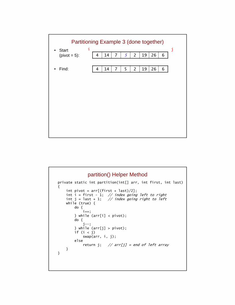
Partitioning Example 3 (done together)
• Start(pivot = 5):
• Find:
4 14 7 5 2 19 26 6
4 14 7 5 2 19 26 6
i j
partition() Helper Methodprivate static int partition(int[] arr, int first, int last) {
int pivot = arr[(first + last)/2];int i = first - 1; // index going left to rightint j = last + 1; // index going right to leftwhile (true) {
do {i++;
} while (arr[i] < pivot);do {
j--;} while (arr[j] > pivot); if (i < j)
swap(arr, i, j);else
return j; // arr[j] = end of left array}
}
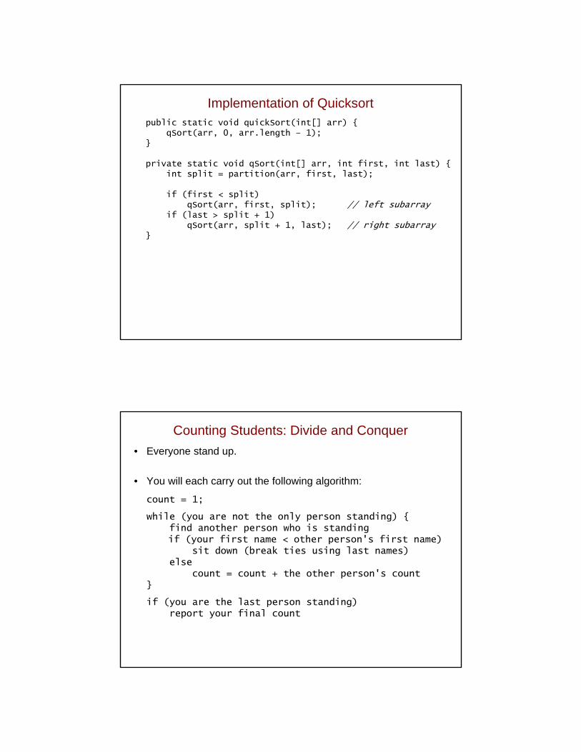
Implementation of Quicksortpublic static void quickSort(int[] arr) {
qSort(arr, 0, arr.length – 1); }
private static void qSort(int[] arr, int first, int last) {int split = partition(arr, first, last);
if (first < split)qSort(arr, first, split); // left subarray
if (last > split + 1)qSort(arr, split + 1, last); // right subarray
}
Counting Students: Divide and Conquer
• Everyone stand up.
• You will each carry out the following algorithm:
count = 1;
while (you are not the only person standing) {find another person who is standingif (your first name < other person's first name)
sit down (break ties using last names)else
count = count + the other person's count}
if (you are the last person standing)report your final count
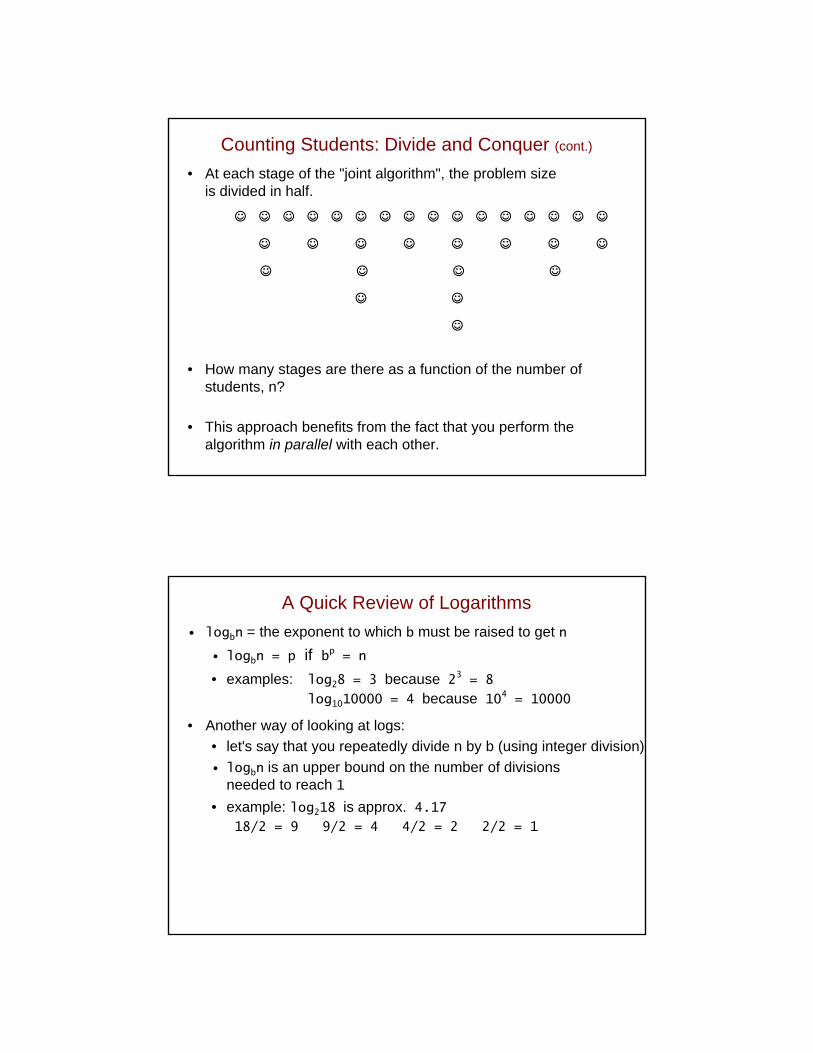
Counting Students: Divide and Conquer (cont.)
• At each stage of the "joint algorithm", the problem size is divided in half.
☺ ☺ ☺ ☺ ☺ ☺ ☺ ☺ ☺ ☺ ☺ ☺ ☺ ☺ ☺ ☺
☺ ☺ ☺ ☺ ☺ ☺ ☺ ☺
☺ ☺ ☺ ☺
☺ ☺
☺
• How many stages are there as a function of the number of students, n?
• This approach benefits from the fact that you perform the algorithm in parallel with each other.
A Quick Review of Logarithms
• logbn = the exponent to which b must be raised to get n
• logbn = p if bp = n
• examples: log28 = 3 because 23 = 8
log1010000 = 4 because 104 = 10000
• Another way of looking at logs:
• let's say that you repeatedly divide n by b (using integer division)
• logbn is an upper bound on the number of divisions needed to reach 1
• example: log218 is approx. 4.17
18/2 = 9 9/2 = 4 4/2 = 2 2/2 = 1
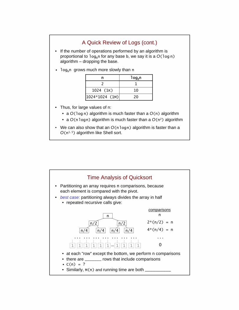
A Quick Review of Logs (cont.)
• If the number of operations performed by an algorithm is proportional to logbn for any base b, we say it is a O(log n)
algorithm – dropping the base.
• logbn grows much more slowly than n
• Thus, for large values of n:
• a O(log n) algorithm is much faster than a O(n) algorithm
• a O(nlogn) algorithm is much faster than a O(n2) algorithm
• We can also show that an O(nlogn) algorithm is faster than a O(n1.5) algorithm like Shell sort.
n log2n
2 1
1024 (1K) 10
1024*1024 (1M) 20
Time Analysis of Quicksort
• Partitioning an array requires n comparisons, because each element is compared with the pivot.
• best case: partitioning always divides the array in half• repeated recursive calls give:
n
2*(n/2) = n
4*(n/4) = n
... ... ... ... ... ... ...
0
• at each "row" except the bottom, we perform n comparisons• there are _______ rows that include comparisons• C(n) = ?
• Similarly, M(n) and running time are both __________
n/2n/2
n/4n/4n/4n/4
1111 1 1 1 1 1
comparisons
...
n
…1
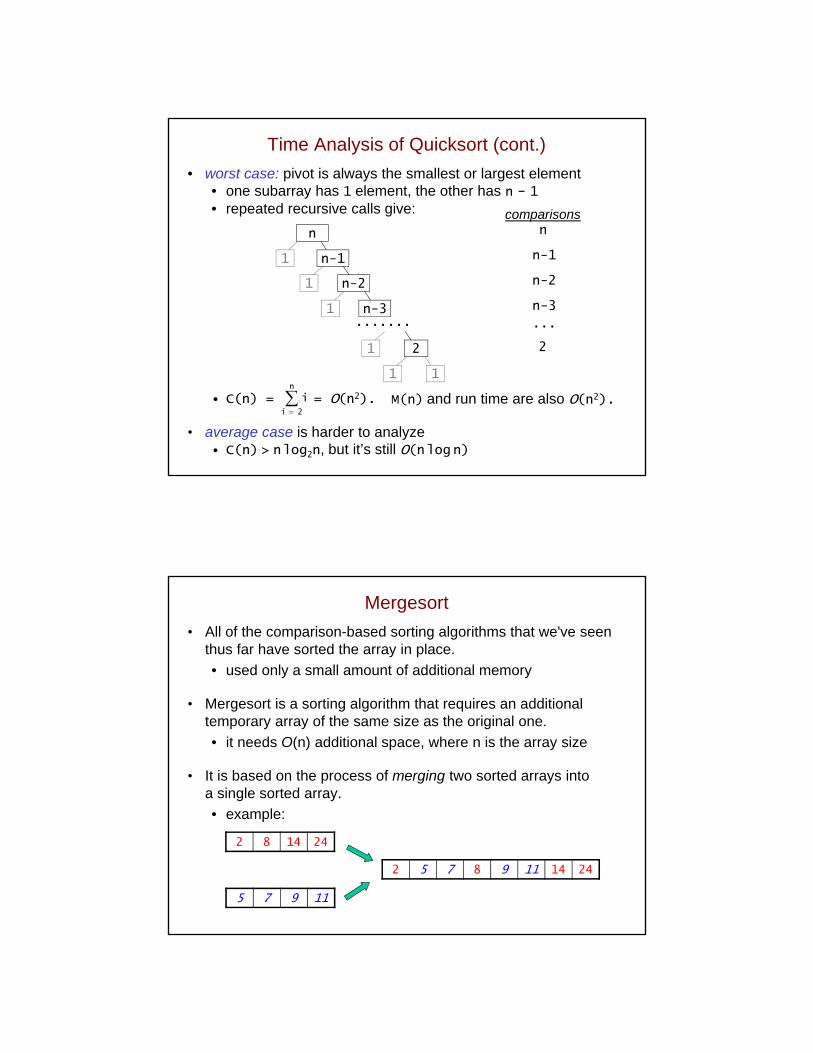
Time Analysis of Quicksort (cont.)
• worst case: pivot is always the smallest or largest element• one subarray has 1 element, the other has n - 1
• repeated recursive calls give:
n
n-1
n-2
n-3.......
2
• C(n) = = O(n2).
• average case is harder to analyze• C(n) > nlog2n, but it’s still O(nlog n)
n-1
n
1
n-21
n-31
1
1 1
...
comparisons
n
2 i
i M(n) and run time are also O(n2).
2
Mergesort
• All of the comparison-based sorting algorithms that we've seen thus far have sorted the array in place.
• used only a small amount of additional memory
• Mergesort is a sorting algorithm that requires an additional temporary array of the same size as the original one.
• it needs O(n) additional space, where n is the array size
• It is based on the process of merging two sorted arrays into a single sorted array.
• example:
5 7 9 11
2 8 14 24
2 5 7 8 9 11 14 24
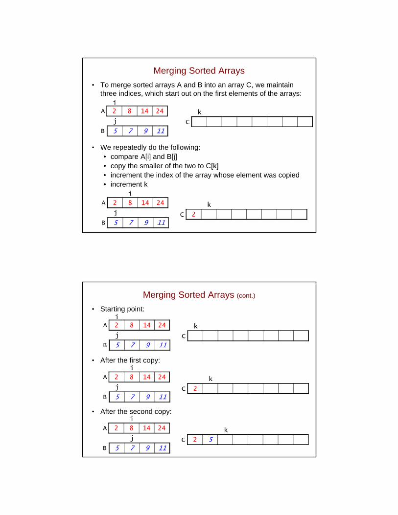
Merging Sorted Arrays
• To merge sorted arrays A and B into an array C, we maintain three indices, which start out on the first elements of the arrays:
• We repeatedly do the following:• compare A[i] and B[j]• copy the smaller of the two to C[k]• increment the index of the array whose element was copied• increment k
2 8 14 24
5 7 9 11
i
j
A
B
C
k
2
2 8 14 24
5 7 9 11
i
j
A
B
C
k
Merging Sorted Arrays (cont.)
• Starting point:
• After the first copy:
• After the second copy:
2 8 14 24
5 7 9 11
i
j
A
B
C
k
2
2 8 14 24
5 7 9 11
i
j
A
B
C
k
2 5
2 8 14 24
5 7 9 11
i
j
A
B
C
k
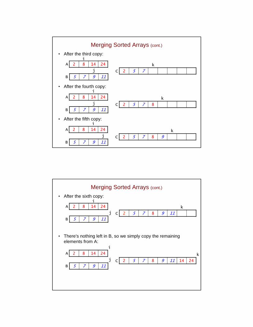
Merging Sorted Arrays (cont.)
• After the third copy:
• After the fourth copy:
• After the fifth copy:
2 5 7
2 8 14 24
5 7 9 11
i
j
A
B
C
k
2 5 7 8
2 8 14 24
5 7 9 11
i
j
A
B
C
k
2 5 7 8 9
2 8 14 24
5 7 9 11
i
j
A
B
C
k
Merging Sorted Arrays (cont.)
• After the sixth copy:
• There's nothing left in B, so we simply copy the remaining elements from A:
2 5 7 8 9 11
2 8 14 24
5 7 9 11
i
j
A
B
C
k
2 5 7 8 9 11 14 24
2 8 14 24
5 7 9 11
i
j
A
B
C
k

Divide and Conquer
• Like quicksort, mergesort is a divide-and-conquer algorithm.
• divide: split the array in half, forming two subarrays
• conquer: apply mergesort recursively to the subarrays, stopping when a subarray has a single element
• combine: merge the sorted subarrays
12 8 14 4 6 33 2 27
12 8 14 4 6 33 2 27
12 8 14 4 6 33 2 27
12 8 14 4 6 33 2 27
8 12 4 14 6 33 2 27
4 8 12 14 2 6 27 33
2 4 6 8 12 14 27 33
split
split
split
merge
merge
merge
Tracing the Calls to Mergesort
12 8 14 4 6 33 2 27
12 8 14 4 6 33 2 27
12 8 14 4
12 8
12 8 14 4 6 33 2 27
12 8 14 4
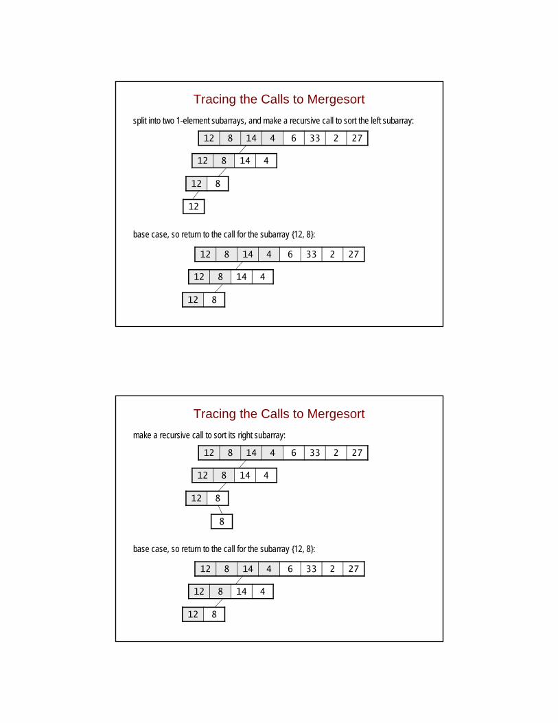
split into two 4-element subarrays, and make a recursive call to sort the left subarray:
split into two 2-element subarrays, and make a recursive call to sort the left subarray:
the initial call is made to sort the entire array:
Tracing the Calls to Mergesort
12 8
12 8 14 4 6 33 2 27
12 8 14 4
12
12 8
12 8 14 4 6 33 2 27
12 8 14 4
base case, so return to the call for the subarray {12, 8}:
split into two 1-element subarrays, and make a recursive call to sort the left subarray:
Tracing the Calls to Mergesort
12 8
12 8 14 4 6 33 2 27
12 8 14 4
12 8
12 8 14 4 6 33 2 27
12 8 14 4
base case, so return to the call for the subarray {12, 8}:
make a recursive call to sort its right subarray:
8
Tracing the Calls to Mergesort
12 8
12 8 14 4 6 33 2 27
12 8 14 4
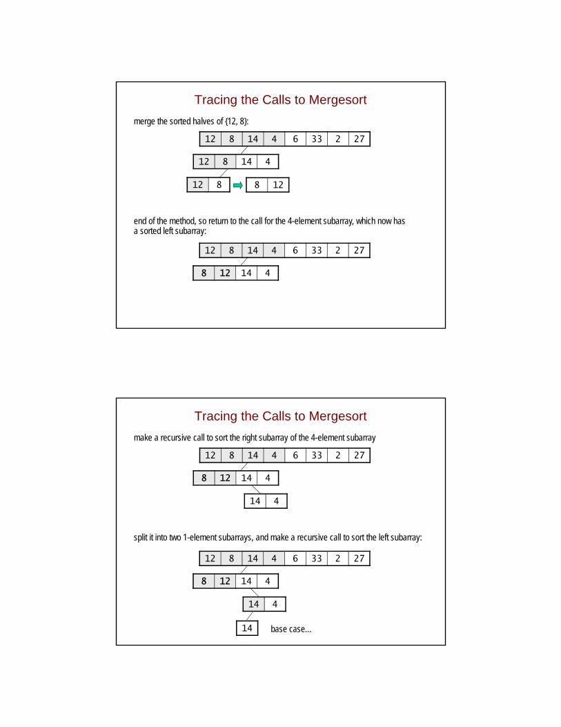
end of the method, so return to the call for the 4-element subarray, which now has a sorted left subarray:
merge the sorted halves of {12, 8}:
8 12
12 8 14 4 6 33 2 27
8 12 14 4
Tracing the Calls to Mergesort
14 4
12 8 14 4 6 33 2 27
8 12 14 4
split it into two 1-element subarrays, and make a recursive call to sort the left subarray:
make a recursive call to sort the right subarray of the 4-element subarray
12 8 14 4 6 33 2 27
8 12 14 4
14 4
14 base case…
Tracing the Calls to Mergesort
14 4
12 8 14 4 6 33 2 27
8 12 14 4
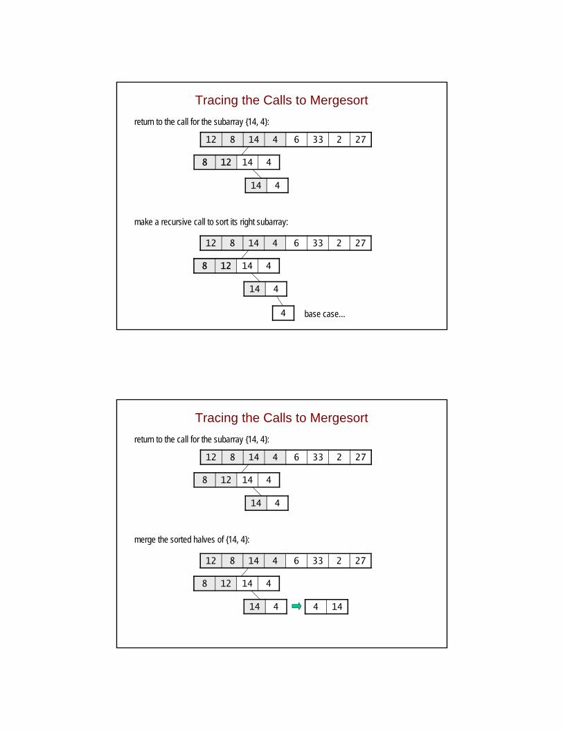
make a recursive call to sort its right subarray:
return to the call for the subarray {14, 4}:
12 8 14 4 6 33 2 27
8 12 14 4
14 4
4 base case…
Tracing the Calls to Mergesort
14 4
12 8 14 4 6 33 2 27
8 12 14 4
merge the sorted halves of {14, 4}:
return to the call for the subarray {14, 4}:
12 8 14 4 6 33 2 27
8 12 14 4
14 4 4 14
Tracing the Calls to Mergesort
12 8 14 4 6 33 2 27
8 12 4 14
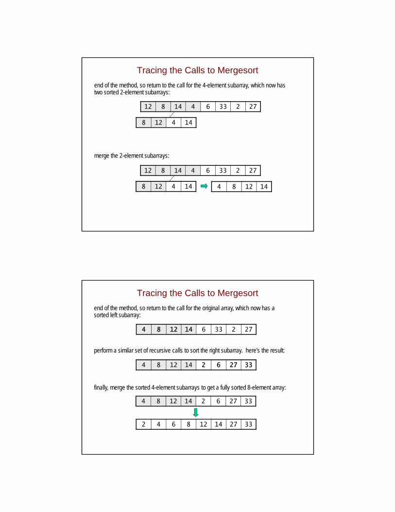
merge the 2-element subarrays:
end of the method, so return to the call for the 4-element subarray, which now has two sorted 2-element subarrays:
12 8 14 4 6 33 2 27
8 12 4 14 4 8 12 14
Tracing the Calls to Mergesort
4 8 12 14 6 33 2 27
perform a similar set of recursive calls to sort the right subarray. here's the result:
end of the method, so return to the call for the original array, which now has a sorted left subarray:
4 8 12 14 2 6 27 33
finally, merge the sorted 4-element subarrays to get a fully sorted 8-element array:
4 8 12 14 2 6 27 33
2 4 6 8 12 14 27 33
Implementing Mergesort
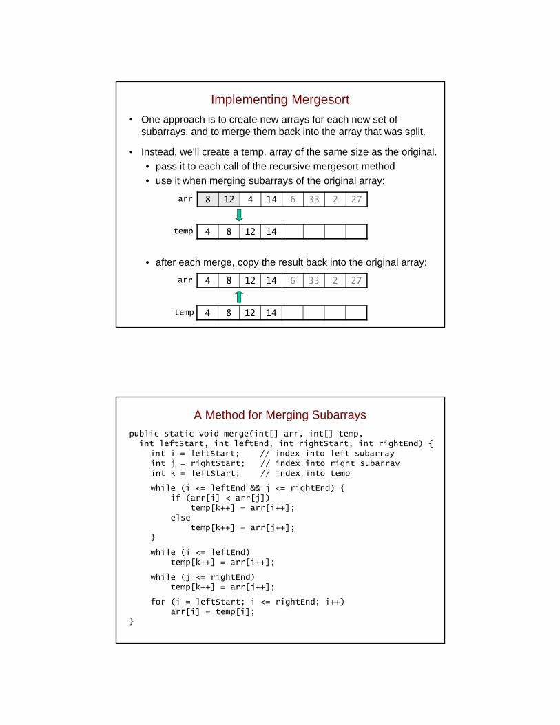
• One approach is to create new arrays for each new set of subarrays, and to merge them back into the array that was split.
• Instead, we'll create a temp. array of the same size as the original.
• pass it to each call of the recursive mergesort method
• use it when merging subarrays of the original array:
• after each merge, copy the result back into the original array:
8 12 4 14 6 33 2 27arr
4 8 12 14temp
4 8 12 14 6 33 2 27arr
4 8 12 14temp
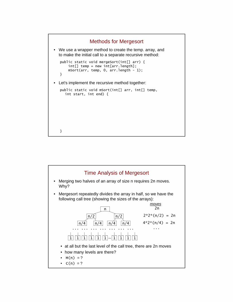
A Method for Merging Subarrays
public static void merge(int[] arr, int[] temp, int leftStart, int leftEnd, int rightStart, int rightEnd) {
int i = leftStart; // index into left subarrayint j = rightStart; // index into right subarrayint k = leftStart; // index into temp
while (i <= leftEnd && j <= rightEnd) {if (arr[i] < arr[j])
temp[k++] = arr[i++];else
temp[k++] = arr[j++];}
while (i <= leftEnd)temp[k++] = arr[i++];
while (j <= rightEnd)temp[k++] = arr[j++];
for (i = leftStart; i <= rightEnd; i++)arr[i] = temp[i];
}
Methods for Mergesort
• We use a wrapper method to create the temp. array, and to make the initial call to a separate recursive method:
public static void mergeSort(int[] arr) {int[] temp = new int[arr.length];mSort(arr, temp, 0, arr.length - 1);
}
• Let's implement the recursive method together:
public static void mSort(int[] arr, int[] temp,int start, int end) { if (start >= end) // base case
return;
int middle = (start + end)/2;mergeSort(arr, tmp, start, middle);mergeSort(arr, tmp, middle + 1, end);
merge(arr, tmp, start, middle, middle + 1, end);}
Time Analysis of Mergesort
• Merging two halves of an array of size n requires 2n moves. Why?
• Mergesort repeatedly divides the array in half, so we have thefollowing call tree (showing the sizes of the arrays):
2n
2*2*(n/2) = 2n
4*2*(n/4) = 2n
... ... ... ... ... ... ...
• at all but the last level of the call tree, there are 2n moves
• how many levels are there?• M(n) = ?
• C(n) = ?
n/2n/2
n/4n/4n/4n/4
11111 1 1 1 1 1
moves
...
n
…
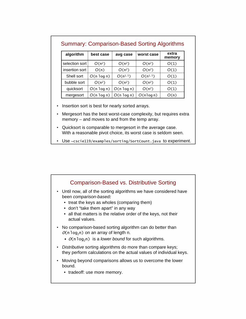
Summary: Comparison-Based Sorting Algorithms
• Insertion sort is best for nearly sorted arrays.
• Mergesort has the best worst-case complexity, but requires extra memory – and moves to and from the temp array.
• Quicksort is comparable to mergesort in the average case. With a reasonable pivot choice, its worst case is seldom seen.
• Use ~cscie119/examples/sorting/SortCount.java to experiment.
algorithm best case avg case worst case extra memory
selection sort O(n2) O(n2) O(n2) O(1)
insertion sort O(n) O(n2) O(n2) O(1)
Shell sort O(n log n) O(n1.5) O(n1.5) O(1)
bubble sort O(n2) O(n2) O(n2) O(1)
quicksort O(n log n) O(n log n) O(n2) O(1)
mergesort O(n log n) O(n log n) O(nlog n) O(n)
Comparison-Based vs. Distributive Sorting
• Until now, all of the sorting algorithms we have considered have been comparison-based:• treat the keys as wholes (comparing them)• don’t “take them apart” in any way• all that matters is the relative order of the keys, not their
actual values.
• No comparison-based sorting algorithm can do better than O(nlog2n) on an array of length n.
• O(nlog2n) is a lower bound for such algorithms.
• Distributive sorting algorithms do more than compare keys; they perform calculations on the actual values of individual keys.
• Moving beyond comparisons allows us to overcome the lower bound.
• tradeoff: use more memory.
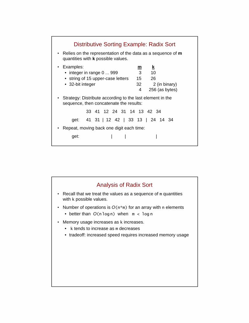
Distributive Sorting Example: Radix Sort
• Relies on the representation of the data as a sequence of m quantities with k possible values.
• Examples: m k• integer in range 0 ... 999 3 10• string of 15 upper-case letters 15 26• 32-bit integer 32 2 (in binary)
4 256 (as bytes)
• Strategy: Distribute according to the last element in the sequence, then concatenate the results:
33 41 12 24 31 14 13 42 34
get: 41 31 | 12 42 | 33 13 | 24 14 34
• Repeat, moving back one digit each time:
get: 12 13 14 | 24 | 31 33 34 | 41 42
Analysis of Radix Sort
• Recall that we treat the values as a sequence of m quantities with k possible values.
• Number of operations is O(n*m) for an array with n elements
• better than O(nlog n) when m < log n
• Memory usage increases as k increases.
• k tends to increase as m decreases
• tradeoff: increased speed requires increased memory usage
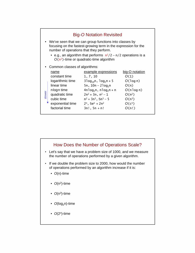
Big-O Notation Revisited
• We've seen that we can group functions into classes by focusing on the fastest-growing term in the expression for thenumber of operations that they perform.
• e.g., an algorithm that performs n2/2 – n/2 operations is a O(n2)-time or quadratic-time algorithm
• Common classes of algorithms:
name example expressions big-O notationconstant time 1, 7, 10 O(1)
logarithmic time 3log10n, log2n + 5 O(log n)
linear time 5n, 10n – 2log2n O(n)
nlogn time 4nlog2n, nlog2n + n O(nlog n)
quadratic time 2n2 + 3n, n2 – 1 O(n2)
cubic time n2 + 3n3, 5n3 – 5 O(n3)
exponential time 2n, 5en + 2n2 O(cn)
factorial time 3n!, 5n + n! O(n!)
slow
er
How Does the Number of Operations Scale?
• Let's say that we have a problem size of 1000, and we measure the number of operations performed by a given algorithm.
• If we double the problem size to 2000, how would the number of operations performed by an algorithm increase if it is:
• O(n)-time
• O(n2)-time
• O(n3)-time
• O(log2n)-time
• O(2n)-time
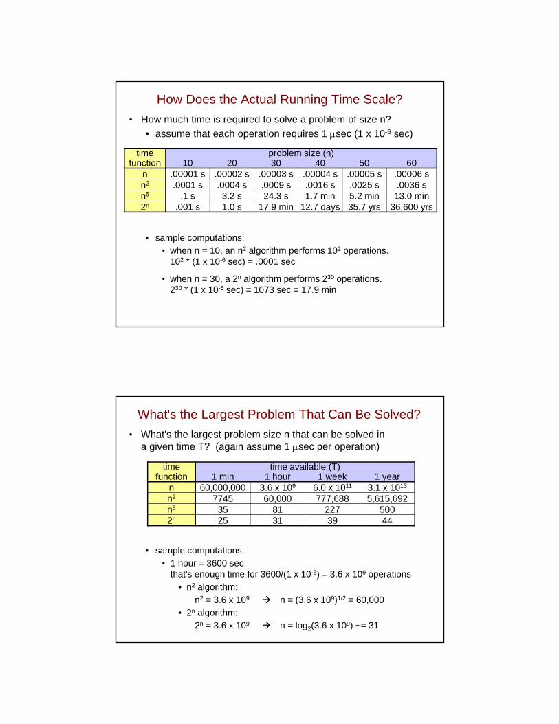
How Does the Actual Running Time Scale?
• How much time is required to solve a problem of size n?
• assume that each operation requires 1 sec (1 x 10⁻⁶ sec)
• sample computations:
• when n = 10, an n2 algorithm performs 102 operations. 102 * (1 x 10-6 sec) = .0001 sec
• when n = 30, a 2n algorithm performs 230 operations.230 * (1 x 10-6 sec) = 1073 sec = 17.9 min
timefunction
problem size (n)10 20 30 40 50 60
n .00001 s .00002 s .00003 s .00004 s .00005 s .00006 sn2 .0001 s .0004 s .0009 s .0016 s .0025 s .0036 sn5 .1 s 3.2 s 24.3 s 1.7 min 5.2 min 13.0 min2n .001 s 1.0 s 17.9 min 12.7 days 35.7 yrs 36,600 yrs
What's the Largest Problem That Can Be Solved?
• What's the largest problem size n that can be solved in a given time T? (again assume 1 sec per operation)
• sample computations:
• 1 hour = 3600 secthat's enough time for 3600/(1 x 10-6) = 3.6 x 10⁹ operations
• n2 algorithm:
n2 = 3.6 x 10⁹ n = (3.6 x 10⁹)1/2 = 60,000
• 2n algorithm:
2n = 3.6 x 10⁹ n = log2(3.6 x 10⁹) ~= 31
timefunction
time available (T)1 min 1 hour 1 week 1 year
n 60,000,000 3.6 x 10⁹ 6.0 x 10¹¹ 3.1 x 10¹³
n2 7745 60,000 777,688 5,615,692n5 35 81 227 5002n 25 31 39 44