south bristol link demand model report - amazon s3 · atkins south bristol link demand model report...

South Bristol Link Demand Model Report April 2013

2

Atkins South Bristol Link Demand Model Report

Notice

This document and its contents have been prepared and are intended solely for North Somerset Council and Bristol City Council’s information and use in relation to the South Bristol Link.

ATKINS Limited assumes no responsibility to any other party in respect of or arising out of or in connection with this document and/or its contents.

Document History

JOB NUMBER: 5103087 DOCUMENT REF: 5103087 - SBL Demand Model Report

Revision Purpose Description Originated Checked Reviewed Authorised Date

1 Draft RJ GB YX TM 30/8/11

2 Final RJ GB YX TM 31/8/11

3 Final LW LW DC GB 26/4/13

3


Table of contents

Chapter pages

1. Introduction 5

Background 5

The Scheme 5

Modelling Suite 6

G-BATS3 6

Key Model Design Considerations 7

Scope of Report 9

2. Demand Model System 10

Introduction 10

DfT Guidance 10

Study Area & Zoning Systems 10

Temporal Scope 13

Segmentation 13

Generalised Cost Formulation 15

Demand Model Structure 16

Model Formulation 18

Modelling Park and Ride 22

Park and Ride Site Allocation 23

Cost Damping 25

Introducing PA-Based Time Period Choice 26

Modelling the Off-Peak Period 30

Demand and Supply Model Outputs 31

3. Model Parameters and Factors 32

Value of Time (VOT) Variation with Distance 32

Factors Derived from Survey Data 33

Fixed Returning Proportions 35

Base Year Bus and Rail Fares 36

4. Demand Model Validation 38

Introduction 38

Convergence Between Supply-Demand 38

Realism Tests 39

Sensitivity Parameters from Realism Tests 44

5. Summary 46

4


Tables

Table 2.1- G-BATS3 and GBATS3 SBLv2 HAM Zoning Systems by Sub-Area 11 Table 2.2 - Demand Model Segmentation 14 Table 2.3 - Demand Model Overview 18 Table 2.4 - Returning Time Period Specification 27 Table 2.5 - Notation Used in PA Formulation 27 Table 3.1 - 2009 Value of Time by Person-Type 32 Table 3.2 - Variation of VOT with Distance 32 Table 3.3 - Demand Segmentation Factors by Purpose/Income (Car) 33 Table 3.4 - Average Bus Purpose Split Factors 33 Table 3.5 - Car Occupancy Factors 34 Table 3.6 - From-home / To-home Factors 34 Table 3.7 - Peak Hour to Peak Period Factors 35 Table 3.8 - CA / NCA Splits for Rail & Bus Users 35 Table 3.9 - Fixed Returning Proportions 35 Table 3.10 - Uplift Factors for PT Fares 37 Table 4.1 - Example of Convergence for Realism Tests 39 Table 4.2 – G-BATS3 SBL Car Fuel Cost Elasticity (WebTAG: -0.1 to -0.4) 40 Table 4.3 – Matrix-Based Car Fuel Cost Elasticity 42 Table 4.4 – Indicators for Strength of Car Fuel Cost Elasticity 42 Table 4.5 - Matrix-based Journey Time Elasticities 43 Table 4.6 – Matrix-based PT Fare Elasticities 43 Table 4.7 - Destination Choice Parameters (Highway) 44 Table 4.8 - Destination Choice Parameters (PT) 44 Table 4.9 - Main Mode / Time Period Choice Parameters 45

Figures

Figure 1.1 South Bristol Link Preferred Option 6 Figure 1.2 – SBL Modelling Chronology 6 Figure 1.3 – SBL v2 Modelling Suite 8 Figure 2.1 - SBL Area of Detailed Modelling 11 Figure 2.2 – G-BATS3 Modelling Suite and G-BATS3 SBL v2 HAM Zoning System 12 Figure 2.3 - Flowchart – Converting 2UC Validated HAM to 6UC SBL Demand Model 14 Figure 2.4 - Demand Model Choice Structure 17 Figure 4.1 - Five Sector Reporting System 41

5


1. Introduction

Background 1.1. The West of England (WEPO) Partnership Organisation local authorities: Bath and North East

Somerset (B&NES), Bristol City (BCC), North Somerset (NSC) and South Gloucestershire Council (SGC) are promoting the South Bristol Link (SBL), a major transport scheme to address current and future transport problems in the south Bristol area.

1.2. Atkins was appointed in April 2010 to undertake Lot 1 – Environmental Impact, of the South Bristol Link package, promoted by North Somerset Council (NSC). The commission has two elements: firstly to support the Best and Final Funding Bid to the Department for Transport and secondly to undertake a full Environmental Impact Assessment [EIA] to support the Environmental Statement [ES] and to represent the Authorities as expert witness at the Public Inquiry

The Scheme 1.3. The proposed development comprises the construction of a section of highway 4.5 kilometres in

length from the A370 Long Ashton bypass within North Somerset to the Hartcliffe (Cater Road) Roundabout within the Bishopsworth area of South Bristol. This incorporates the minor realignment of sections of existing highway at Highridge Green, King George’s Road and Whitchurch Lane. The entire route is to be classed as an Urban All-Purpose Road (UAP) in accordance with TA 79/99.

1.4. The route includes the construction of new junctions with the A370, Brookgate Road, A38, Highridge Road, Queens Road and Hareclive Road. New bridges will be constructed to cross Ashton Brook, Colliter’s Brook and to pass under the Bristol to Taunton Railway Line. The route corridor will incorporate a bus-only link to connect with the Ashton Vale to Temple Meads (AVTM) spur into the Long Ashton Park and Ride site, and dedicated bus lanes between the railway and the new A38 roundabout junction. New bus stops and shelters, and a continuous shared cycleway and footway will be provided along the route corridor. Associated proposals include drainage facilities, landscaping and planting.

Figure 1.1 – SBL Scheme

6


1.5. The route will form part of the West of England rapid transit network (Metro Bus) and will be used by buses and other motorised vehicles. The route will link with the AVTM at the Long Ashton Park and Ride site, and within the South Bristol section, once buses have reached the Hartcliffe Roundabout, services will follow existing roads via Hengrove Way to Imperial Park and onwards to Whitchurch Lane and Hengrove Park.

Modelling Suite 1.6. The SBL traffic forecasts have been undertaken using various models, with each model an

update on the previous version, bringing improvements to the specific area to the south of Bristol and ensuring that the model performance and geographic scope is appropriate for testing the scheme. The chronology of the models used is shown in Figure1.2 and the elements are described below.

Figure 1.2 – SBL Modelling Chronology

G-BATS3 1.7. The G-BATS3 modelling suite has 600 zones; covers the Bristol area; has a 2012 base year

and consists of:

a Highway Assignment Model (G-BATS3 HAM) representing vehicle-based movements across the Greater Bristol Area for a typical 2012 morning peak hour (08:00 – 09:00), an average inter-peak hour (10:00 – 16:00) and an evening peak hour (17:00 – 18:00);

a Public Transport Assignment Model (G-BATS3 PTAM) representing bus and rail-based movements across the same area and time periods in 2012; and

a five-stage multi-modal incremental Demand Model (G-BATS3 DM) that estimates frequency choice, main mode choice, time period choice, destination choice, and sub mode choice in response to changes in generalised costs across the 24-hour period (07:00 – 07:00).

1.8. The GBATS3 modelling suite was the starting point for the modelling of the G-BATS3 SBL model, although this was updated to a 2012 base year and extended to include 632 zones in the assignment models.

7


1.9. Following comments from DfT during the submission of the SBL BAFB, further revisions to the G-BATS3 SBL model have been made. These revisions involve updates to the demand model and a completely revised highway assignment model (HAM). The revisions to the G-BATS SBLv2 DM comprised re-calibrating and re-validating the G-BATS3 SBLv3 DM that now incorporates the new G-BATS3 SBLv3 HAM.

Key Model Design Considerations 1.10. The interaction between the different models for the purpose of appraising the SBL using the

SBL v3 modelling suite is shown in Figure 2.2.

Demand Model

1.11. The G-BATS3 model is a 24-hour demand model. Compliant with WebTAG, it is an incremental demand modelling approach which responds to changes in costs, measured in generalised minutes.

Highway Model

1.12. The SBL Highway Assignment Model (HAM) is an integral part of the demand modelling process as it undertakes the highway assignment that in turn provides highway costs to the demand model. The highway model is SATURN based and has been established for a 2012 base year.

Public Transport Model

1.13. The SBL Public Transport Model (PTAM) includes all bus and rail services serving the Bristol urban area. The model is EMME based and has been established for a 2012 base year.

8


Figure 1.3 – SBL v2 Modelling Suite

9


Scope of Report 1.14. This Model Development Report consists of five sections. Following this introductory section:

Section Two describes the structure of the demand model and its functional forms;

Section Three presents parameters derived from the 2012 survey data to build the G-BATS3 SBL base demand model, such as segmentation factors, and Value of Time (VOT) parameters as well as the VOT variation with distance for HBO and NHBO trips;

Section Four provides convergence statistics and realism test results, including highway fuel cost elasticities and PT fare elasticities by purpose, time period and person type, and derived sensitivity parameters and scale theta parameters; and

a summary of the model development is presented in Section Five.

10


2. Demand Model System

Introduction 2.1. The G-BATS3 SBL v3 demand model is fundamentally the same as the G-BATS3 demand

model (and is referred to as the ‘demand model’ in the rest of the report) and was developed to appraise a wide range of transport options that could be implemented in the sub-region. This includes schemes such as highway improvements, demand management and parking charges as well as bus rapid transit, rail, park and ride, and traffic management schemes.

2.2. The demand model represents travel choices across a typical 24-hour weekday period explicitly representing an AM peak period (07:00 – 10:00), an Inter-Peak period (10:00 – 16:00), a PM Peak period (16:00 – 19:00), and an off-Peak period (19:00 – 07:00).

2.3. The demand model is a variable demand model in an incremental hierarchical form, pivoting off the base year, and estimating the choice between travel alternatives (frequency, modes, time periods, and destinations) depending on the change of generalised costs or disutility.

2.4. The demand model uses a Production – Attraction (PA) formulation as recommended in WebTAG Unit 3.10.2. It also includes variation of the Value of Time (VOT) with trip length for non-Work trips.

2.5. External to external movements are considered as fixed movements along with goods vehicle movements, and therefore these are not modelled in the demand model.

2.6. The model was been developed in a modular fashion to enable subsequent adaptation in response to further updates and refinement.

DfT Guidance 2.7. The design of the demand model closely follows the latest DfT WebTAG guidance. In particular,

the development of the demand model is in compliance with:

WebTAG Unit 3.10.1 to 3.10.4 - Variable Demand Modelling;

WebTAG Unit 3.11 - Modelling of Public Transport Schemes; and

WebTAG Unit 3.12.2c - Design, Modelling and Appraisal of Road Pricing Schemes.

Study Area & Zoning Systems 2.8. The G-BATS3 modelled area covers the greater Bristol urban area and its environs, extending

approximately to the boundary of the former county of Avon. The main focus of the model is on Bristol City Centre and the surrounding urban area. This is bounded to the west by the M5, to the North by the M4 - with an extension along the A432 to Yate - to the east by the A4174 outer ring road - with an extension to include Keynsham and Cadbury Heath - and to the south by the edge of the Bristol City Boundary, running in an arc from the A4/A4174 junction to the A370 at Long Ashton. A detailed zoning system has been defined to represent this area. Outside the study area – termed the external area – a less detailed zone system has been defined. This covers the area immediately around the study area and also extends to cover the rest of the UK.

2.9. The SBL area of detailed modelling is shown in Figure 2.1, and was determined from the earlier SBL Option Identification Study which showed the extent to which the introduction of the proposed SBL scheme influenced the flows within the full G-BATS3 modelled area, and is bounded by:

City centre to the north;

A37 to the east;

A369 to the west; and

B3130 to the south

11


Figure 2.1 - SBL Area of Detailed Modelling

G-BATS3 Modelling Suite Zoning System

2.10. The G-BATS3 modelling suite zoning system comprises 600 zones covering the whole of Great Britain. A detailed zoning system was developed to represent the Greater Bristol Urban area and its surroundings. The zoning system also includes 10 Park and Ride zones (of which three are already in operation) as well as separate development zones.

SBL Zoning System

2.11. The G-BATS3 SBLv2 zoning system is based on the G-BATS3 modelling suite zoning system, but has been enhanced in the SBL area of detailed modelling, taking account of the SBL scheme alignment, increasing the total number of zones from 600 to 632. The new zones were formed by subdividing G-BATS3 zones as this facilitates the transfer of data between the G-BATS3 SBLv3 HAM AND G-BATS3 SBLv3 DM.

Comparison of G-BATS3 and SBL Zoning Systems

2.12. The G-BATS3 SBLv3 HAM and G-BATS3 modelling suite zone systems are shown Table 4.1 alongside the alignment of the SBL, with G-BATS3 zone boundaries shown in black and SBL zone boundaries in red – note that the zoning is unchanged from that used for G-BATS3 outside of the SBL area of detailed modelling shown in the diagram.

Table 2.1- G-BATS3 and GBATS3 SBLv3 HAM Zoning Systems by Sub-Area

Area G-BATS 3 SBL v3 HAM GBATS3

Bristol 287 274

North Somerset 63 62

B&NES 36 36

South Gloucestershire 162 162

External 46 46

Unallocated in base year 38 20

Totals 632 600

12


Figure 2.2 – G-BATS3 Modelling Suite and G-BATS3 SBL v3 HAM Zoning System

Model Zoning Systems

G-BATS3

SBL

Contains Ordnance Survey data © Crown copyright and database right 2012

13


Temporal Scope 2.13. The demand model is a 24-hour demand model representing four time periods: the morning

peak (AM), the inter-peak (IP), the evening peak (PM) and the off-peak (OP) period, starting from 07:00 and concluding at 07:00 the following day.

2.14. The relationships between the various peak periods and peak hours are defined as follows:

AM peak period: 07:00 - 10:00;

AM peak hour (for assignment modelling only): 08:00 - 09:00;

Inter-peak period: 10:00 - 16:00;

Inter-peak hour (for assignment modelling only): 1/6th of 10:00 - 16:00;

PM peak period: 16:00 - 19:00;

PM peak hour (for assignment modelling only): 17:00 - 18:00; and

Off Peak period: 19:00 - 07:00 (but without assignment). Note that the AM and PM peak hours are not the average of AM and PM peak period hours.

2.15. The definition of the modelled time periods has been informed by the discussion in WebTAG Unit 3.10.2, paras 1.8.8 - 1.8.16, with time period choice (within the demand model) undertaken at the peak period level whilst a specific AM peak hour, inter-peak (IP) hour and PM peak hour is used in the assignment.

Segmentation

Within the Demand Model

2.16. Travel demands in the demand model were segmented by car availability and journey purpose as described below:

By person type

Car available (CA); and

Non-car available (NCA).

By household income

Income Low (IL): less than £17,500;

Income Medium (IM): £17,500 to £35,000; and

Income High (IH): greater than £35,000.

By journey purpose

Home based work (HBW);

Home based other (HBO);

Non-home based other (NHBO);

Home based employer’s business (HBEB); and

Non-home based employer’s business (NHBEB).

2.17. Table 2.2 shows the segmentation undertaken within the demand model. Overall, there are 16 demand segments including the income segments which are reserved for future user charging development. Note that the work trips (i.e. HBEB and NHBEB) and NCA trips are not segmented by income band.

14


Table 2.2 - Demand Model Segmentation

Supply Purpose

Demand Purpose

Car Available (CA) Non Car Available (CA)

<£17,500 £17,500 to £35,000

> £35,000

Commuting HBW 8 9 10 15

Other HBO 0 1 2 11

NHBO 3 4 5 12

Work HBEB 7 14

NHBEB 6 13

Note: the numbers shown above refer to the segment ID used within the demand model.

Within the Highway Assignment

2.18. The G-BATS3 SBL V3 HAM segmentation was undertaken in a more aggregated form than that adopted for the demand models to reduce the model runtimes. The G-BATS3 SBL v3 HAM was validated to two user classes. A detailed flowchart describing the conversion process of a validated G-BATS3 SBL v3 HAM into six user classes is shown in Figure 2.3.

Figure 2.3 - Flowchart – Converting 3UC Validated HAM to 6UC SBL Demand Model

15


2.19. The goods vehicle movements for LGV and HGV are not considered within the demand model. As suggested by WebTAG Unit 3.10.1, para 1.2.5, their forecast year trip matrices did not change in response to cost changes.

Within the Public Transport Assignment

2.20. Within the EMME-based Public Transport assignment models, no distinction was made between journeys undertaken for different purposes, household income bands or car availability. Instead, the overall public transport demand was allocated (by logit-based choice mechanisms) to the various PT sub-modes, where available:

Rail; and

Bus / BRT.

Generalised Cost Formulation

Private Car

2.21. WebTAG Unit 3.10.2 defines the generalised cost for private car person trips and includes elements relating to:

fuel cost;

in-vehicle time;

parking costs;

access/egress time; and

tolls or other user charges.

2.22. The demand model follows the WebTAG formula for the definition of generalised costs for cars: Gcar , measured in units of time-minutes:

Gcar = Vwk*A + T + D*VOC/(occ*VOT) + PC/(occ*VOT)

where:

Vwk is the weight applied to walking time (assumed 0 currently);

A is the total walk time to/from the car (minutes);

T is the journey time spent in the car (minutes);

D is the motorised journey length (kilometres);

VOC is the vehicle operating cost (pence per km): including the fuel and non-fuel

operating cost for the work purposes but only the fuel operating cost for non-work

purposes;

occ is the occupancy (i.e. the number of people in the car) who are assumed to

share the cost;

VOT is the appropriate Value of Time (pence per minute); and

PC is the parking cost and tolls (if and when incurred), in monetary units (pence).

2.23. WebTAG Unit 3.5.6 provides guidance for calculating Values of Time and vehicle operating costs for general scheme appraisal and assessment whilst WebTAG Unit 3.12.2 Annex A provides guidance on segmentation and values of time for road pricing models. Values of vehicle operating costs (VOC), values of time (VOT) and occupancy (occ) have been derived from WebTAG Unit 3.5.6 (April 2009).

16


Public Transport

2.24. WebTAG Unit 3.10.2 defines the generalised cost for public transport users and includes elements relating to:

fares;

in-vehicle time;

walking time to and from the service;

waiting times; and

interchange penalty.

2.25. The WebTAG formula for PT generalist cost GPT, measured in units of time (minutes) is given as:

GPT = Vwk*A + Vwt*W + T +F/VOT + I

where:

Vwk (=2) is the weight applied to time spent walking;

A is the total walking time to and from the service;

Vwt (=2.5) is the weight applied to time spent waiting;

W is the total waiting time for all services used on the journey;

T is the total in-vehicle time;

F is total fare;

VOT is the appropriate Value of Time, in pence per minute; and

I (=10 minutes) is the interchange penalty if the journey involves transferring from

one service to another.

2.26. The above weights 2 and 2.5 are the standard values provided in WebTAG Unit 3.11.2.

Demand Model Structure 2.27. The G-BATS3 demand model has a hierarchical logit choice structure as shown in Figure 2.4.

Compliant with WebTAG, an incremental demand modelling approach was adopted which responds to changes from the base year generalised costs, measured in generalised minutes.

17


Figure 2.4 - Demand Model Choice Structure

2.28. The sub-mode choice between bus, BRT and LRT (if any) is undertaken by the public transport assignment, i.e. they are within the same segmentation in the demand model.

2.29. The P&R sub-mode is a highway sub mode which means that P&R generally extracts more patronage from cars. The P&R extraction from bus-all-the-way is modelled implicitly by the main mode choice, up and down the demand model hierarchical tree via the destination choice and the time period choice as shown in Figure 2.4.

2.30. An overview of the model stages, functional forms (e.g. OD/PA and Car-Available / Non-Car Available) and time periods is listed in Table 2.3 for each of the six stages in the demand modelling. Note that:

Stages 1 to 5 are undertaken within the demand model whilst stage 6 is provided

through the separate highway and public transport assignment models; and

the public transport sub-mode choice is undertaken within the demand model.

2.31. Frequency choice is included as the model does not allow for slow modes such as walking and cycling. The frequency modelling (stage 1) is undertaken for HBO and NHBO trips only, as trips of these purposes are typically more elastic to changes in costs. As suggested by WebTAG Unit 3.10.3 para 1.11.9, no frequency response is included for commuting or employer's business trips.

2.32. The main mode choice (stage 2) between car and PT operates for the Car Available (CA) person type only. The demand model operates at the 24-hour level until the time period choice (stage 3) is undertaken. For destination choice modelling (stage 4), the demand model considers all four time periods AM/IP/PM/OP for all person types in parallel. The resulting PA

Trip Frequency

Main Mode Choice

Time Period Choice

Destination Choice Destination Choice

Time Period Choice

Public Transport Car / Park & Ride

Sub - Mode Choice Sub - Mode Choice

Car Rail Park &

Ride

Bus/BRT

18


matrices are converted into OD matrices after the sub-mode choice (stage 5) and before the individual highway and PT assignments (stage 6) are undertaken.

Table 2.3 - Demand Model Overview

Stage Model Temporal Scope Form Person Type

1 Frequency Modelling 24-hour PA Trip Ends All (CA & NCA)

2 Main Mode Choice 24-hour PA Trip Ends CA

3 Time Period Choice Translate 24-hour to AM (3hr), IP (6hr), PM (3hr) and OP (12hr) periods

PA Trip Ends CA & NCA

4 Destination Choice 3hr (AM), 6hr (IP), PM (3hr) and OP (12hr)

Translate PA Trip Ends to PA matrices

All (CA & NCA)

5 Sub-Mode Choice 3hr (AM), 6hr (IP), PM (3hr) and OP (12hr)

PA matrices All (CA & NCA)

6 Assignment 1-hour OD matrices All (CA & NCA)

Model Formulation

Incremental Logit-based

2.33. The choice modelling for various demand responses follows an incremental approach as required by WebTAG, pivoted off the base year situation. The logit-based formulation is described below for each of the five demand modelling stages.

2.34. The demand model is implemented in terms of utilities and composite utilities consistent with the WebTAG hierarchical logit (HL) formulation (WebTAG Unit 310.3, Appendix 4). The formulae given below are specified in terms of the WebTAG HL tree structure, i.e. using lambda parameters for the lower level sub-mode choice and destination choice but using theta parameters for the upper level time period choice, main mode choice and the trip frequency modelling.

Frequency Modelling

2.35. The demand model does not explicitly model ‘slow’ modes (i.e. walking and cycling) and WebTAG suggests that it may be logical to consider some form of frequency modelling within the demand model (WebTAG Unit 3.10.3, paras 1.7.17 -1.7.18). WebTAG does not provide illustrative parameters for frequency other than noting its position within the demand model structure. The lambda values for the frequency parameters were set during the realism tests and adjusted, through an iterative process, in order to achieve the target elasticities.

2.36. The formula for the frequency modelling is as follows

ipcfreq U

ipcipc eTT

*0

where:

i : production end; p: purpose; c: person type such as CA, NCA, or income

segment;

0

ipcT: reference zonal production over i.p.c;

ipcT: output zonal production over i.p.c;

freq: frequency choice structure (or scale) parameter; and

19


m ipc

C

ipcmipc TeTU ipcmm 00 /ln(

: logsum of lower level main mode choice,

where m is mode.

2.37. WebTAG recommends that frequency modelling is undertaken for HBO and NHBO purposes only. The frequency modelling structure theta parameter is 0.05 for both purposes (HBO and NHBO) and for both person types (CA and NCA), derived from realism testing.

Main Mode Choice

2.38. WebTAG (Unit 3.10.2) suggests that the main mode choice between cars and public transport for car available travellers should be placed just below the frequency modelling in the choice hierarchy, whilst the time period choice should be placed at a level similar to main mode choice.

2.39. The formula for the main mode choice is as follows:

k

U

ipck

U

ipcm

ipcipcmipckm

ipcmm

eT

eTTT

0

0

where:

i: production end; p: purpose; c: person type; m: main mode (car or PT); k: used

for summation over main modes car and PT;

production trip ends over i.p.c.m;

ipcmT: output zonal production trip ends over i.p.c.m;

0

ipcmT: reference zonal production trip ends over i.p.c.m;

m : main mode choice sensitivity parameter

ipcT: input zonal production trip ends over i.p.c from the above frequency stage;

t ipcm

U

ipcmtipcm TeTU ipcmtt 00 /ln(

: logsum of lower level time period

choice, where t is time period.

Time Period Choice

2.40. WebTAG (Unit 3.10.2) suggests that time period choice parameter values should be similar in magnitude to main mode choice parameter values. The scale parameters used for the time period choice were set to the same value as used in main mode choice – in mathematical terms, they are modelled simultaneously in a multinomial form.

2.41. The formula for the time period choice between the four periods (i.e. AM, IP, PM and OP period) is as follows:

k

U

ipcmk

U

ipcmt

ipcmipcmtipcmkt

ipcmtt

eT

eTTT

0

0

where:

t: time period; k: used for summation over time periods AM, IP, PM and OP;

0

ipcmtT: reference zonal production trip ends over i.p.c.m.t;

20


ipcmT: input zonal production trip ends over i.p.c.m from the above mode choice

stage;

t : time period choice tree structure scale parameter;

j ipcmt

U

ijpcmtipcmt TeTU ijpcmtdist 00 /ln(

: logsum of lower level summed over

all attractions j, singly constrained destination choice for HBO, NHBO, NHBEB,

and HBEB purposes; and

j ipcmt

U

ijpcmtjpipcmt TeTBU ijpcmtdist 00 /ln(

: logsum of lower level, doubly

constrained destination choice for HBW purpose only.

2.42. However, the estimation of the logsum ipcmtU for the doubly constrained distribution was not

as straightforward - further details are provided below.

Destination Choice

2.43. WebTAG (Unit 3.10.2) recommends that the destination choice should be modelled as singly (origin) constrained distribution for trips with HBO, NHBO, NHBEB or HBEB purposes. In contrast, WebTAG recommends that the destination choice for HBW should be modelled as doubly (i.e. origin-and-destination) constrained distribution. To meet this requirement, a rectangular Furnessing procedure was developed to undertake the HBW distribution modelling.

2.44. The formula for the singly constrained destination choice was:

k

U

ikpcmt

U

ijpcmt

ipcmtijpcmtikpcmtdist

ijpcmtdist

eT

eTTT

0

0

where:

j : attraction end; k: numeration of all destinations;

0

ijpcmtT: reference PA matrix over p.c.m.t;

ipcmtT: input zonal production trip ends over i.p.c.m.t from the above time period

choice;

dist: destination choice sensitivity parameter;

ijpcmtT: output PA matrix over p.c.m.t; and

)/ln( 00

s ijpcmt

C

ijpcmtsijpcmt TeTU ijpcmtssub

: logsum of lower level sub- mode

choice, summed over all sub-modes S.

2.45. All distribution models, irrespective of whether they are singly or doubly constrained, satisfy the following row constraints:

j ijpcmtipcmt TT .

2.46. For doubly constrained distribution, another set of column constraints is also introduced:

imtc ijpcmtimtc ijpcmt TT 0

.

2.47. The adopted rectangular Furnessing procedure guarantees that the above two sets of constraints are always satisfied. In other words, each zone attracts a fixed amount of (total) trips for each person type within a purpose.

21


2.48. The formula for the doubly constrained distribution is

k

U

ikpcmtkp

U

ijpcmtjp

ipcmtijpcmtikpcmtdist

ijpcmtdist

eTB

eTBTT

0

0

where:

j : attraction end; k: used for summation over all destinations;

0

ijpcmtT: reference PA matrix over p.c.m.t;

ipcmtT: input zonal production trip ends over i.p.c.m.t;

dist: destination choice sensitivity parameter;

jpB: attraction balance factors for purpose p and destination j, estimated via the

rectangular Furnessing procedure;

ijpcmtT: output PA matrix over p.c.m.t;

)/ln( 00

s ijpcmt

U

ijpcmtsijpcmt TeTU ijpcmtssub

: logsum of sub mode choice

2.49. Note that the attraction balance factors were estimated via inner loops between this distribution stage and the above time period choice and main mode choice. This was necessary because

the trip ends from the above two stages were a function of the logsum (or jpB) of this doubly

constrained stage, which in turn, was a function of the Furnessing procedure for jpB,

dependent on the resulting forecast trip ends from the above two stages.

2.50. The initial values for the inner loops were:

j ijpcmtipcmt TT 0

, ,1ipcmt and jpB

=1,

where ipcmt are the row balance factors to ensure doubly constrained distribution

satisfied.

2.51. Note that within the inner loops, before the logsum is evaluated, the attraction balance factors

are normalised such that ,

j jp NBwhere N = number of zones with non-zero attractions.

Sub-Mode Choice

2.52. After destination choice, the sub-mode choices is undertaken for highway and public transport users independently.

2.53. Park and Ride (P&R) users appeared in the single nest of sub-mode choices (as previously shown in Figure 2.4), to facilitate the sub-mode switching in forecast years between highway and P&R only.

2.54. The formula for the sub mode choice was:

k

U

ijpcmts

U

ijpcmts

ijpcmtijpcmtsijpcmtssub

ijpcmtssub

eT

eTTT

0

0

where:

22


s: sub-mode, k: used for summation over highway submodes car and P&R, or

PT sub-modes rail, bus;

0

ijpcmtsT: reference PA matrix over p.c.m.t;

ijpcmtT: input PA matrix over p.c.m.t from the above destination choice;

sub: sub-mode choice sensitivity parameter;

ijpcmtsT: output PA matrix over p.c.m.t.s;

)( 0

ijpcmtsbijpcmtsbsubijpcmts CCU : the change in generalised costs at the lowest

level of the hierarchy.

2.55. WebTAG does not provide explicit values to be used for the sub-mode choice scale parameter lambda. Similar models developed by Atkins have used a value around -0.1. The G-BATS3 SBL demand model adopts the same value of -01 for both highway and PT sub mode choice.

2.56. Note that the bottom level ijpcmtsUis subject to damping to overcome the oversensitivity for

long distance trips. This arises because the elasticity of logit formulation scales with the disutility - longer distance trips exhibit larger cost differences producing unrealistically high elasticities, if costs are not scaled. More details of the cost damping functions used in G-BATS3 are given below.

Modelling Park and Ride 2.57. Modelling park and ride (P&R, a highway sub-mode) raises a number of issues as it requires

linking highway and public transport elements of the model. This section sets out the modelling methodologies implemented in the G-BATS3 demand model.

2.58. WebTAG Unit 3.10.7 advises that for models where evidence from a local estimation is not available, the positioning of park-and-ride choice as a sub-mode of either car or public transport may be based on the following:

where park-and-ride is dominated by relatively short car legs in order to gain

access to a substantial public transport leg, then positioning as a sub-mode of

public transport is likely to be the more appropriate; and

where the park-and-ride site is located so as to attract relatively long car trips to

change mode on the edge of the urban area, and where public transport mode

share is low for the movements of interest, then treatment as a sub-mode of car

is likely to be the more appropriate.

2.59. Within the Bristol area the park and ride sites are located as such to intercept relatively long car journeys on the edge of the urban area. As such, park-and-ride choice is a sub-mode of either car in the G-BATS demand model.

2.60. There are four key stages in the P&R modelling approach:

derivation of park and ride generalised costs;

estimation of park and ride demand in the demand model;

site allocation of park and ride demand to competing sites; and

assignment of highway and PT legs of park and ride trips to the networks.

2.61. P&R sites are defined in the model as individual zones. The P&R modelling is undertaken via a definition of catchment areas for each P&R zone. This restriction on P&R movements on home locations reflects what is likely in reality where users normally use sites that are convenient to them (e.g. travellers from the north of a city are most likely to use a site on the north side of the city).

23


Deriving Park and Ride Generalised Costs

2.62. The highway and PT network models are used to define the generalised cost for a park and ride journey between zone to zone pairs.

2.63. P&R sites are defined in the model as individual zones. In the base case there are three existing bus P&R zones as listed below1:

A4 Portway (Avonmouth): bus P&R site;

Brislington: bus P&R site; and

Long Ashton: bus P&R site.

2.64. A number of P&R zones are reserved for potential future applications; it is possible to define different park and ride sites for those identified as “proposed” providing the new zone is appropriately located in the highway and PT networks.

2.65. The highway network model (SATURN) is used to determine travel times and costs from production zones to each park and ride site (zone). The PT network model (Emme) is used to determine travel times and costs from the park and ride zones to each attraction zone.

2.66. The park and ride generalised cost for a given production to attraction zone movement is determined by taking the minimum combination of highway plus PT costs also taking into account a parking charge, PT fare and site specific constant.

2.67. In model application only those sites considered active are used in the process (i.e. even though additional zones are defined for possible sites they are only used if a site is assumed in place in a given forecast model run).

2.68. It is noted that this process is undertaken to derive park and ride generalised costs for all car-available demand segments by purpose, income group (if modelled), and modelled time period.

Application in the Demand Model

2.69. The park and ride generalised costs are passed to the demand model. As shown in Figure 2.4, park and ride appears in the bottom of the car nest of the main mode choice, and is not treated as a PT sub-mode. The model has a typical binary logit structure with the following to note:

The main demand model uses the minimum generalised cost (between a

production and attraction zone pair through a P&R site) to determine overall park

and ride demand for all sites; and

The scaling parameter subused at this level is set slightly higher than (or equal

to) the destination sensitivity choice parameter dist, and is typically about 0.1 (in

generalised minutes). There is no current guidance on lambda values of sub

mode choice -- sensitivity tests may be needed if a higher value is set.

2.70. The demand model structure passes composite costs up from the lower levels to higher levels, so park and ride generalised costs have an influence on destination choice, time period choice and main mode choice.

Park and Ride Site Allocation 2.71. Outside the main demand model an independent park and ride site choice module is

implemented. As described above the main demand model works using the generalised cost estimated for the least cost park and ride site. However, some overlap of site catchment areas occurs now and can be expected to occur with new site locations. The allocation model therefore takes the park and ride demand from the main demand model and examines the

1 Note: An informal Park & Rail is also available at Bristol Parkway Station but without any dedicated P&R

facilities and any reliable survey data on passenger volumes. In this case, P&R is simply modelled as the cheapest mode (ie by bus or rail) versus car in terms of overall generalised cost.

24


generalised cost of travel to different potential sites for every production-attraction pair. This model is especially important when a number of sites are close alternatives.

2.72. The allocation of park and ride between competing sites is modelled also using a logit model, where demand at a site is a function of the average generalised cost between the zones in each catchment area to the available sites and between these sites to the central business district (CBD):

k

CwC

CwC

c

pqprqPTkqk

carpk

PTrqr

carpr

e

eDD

321

321

where:

r : Park & Ride site under consideration;

k : used for summation over all Park & Ride sites

1

= 0.02, 2

= 0.02, and 3

= 0.01;

pkqD: P&R trips from p to q using site r;

c

pqD: input aggregated P&R matrix from the above highway and PT sub mode

choice;

car

prC

: average generalised car costs (mins) from origin p to site r;

PT

rqC

: average generalised PT costs (mins) from site r to final destination q

rw

: the total cost of parking (mins) at site r, including site penalties (currently

assumed to equate to a cost of six generalised minutes), bus fare and site

specific constants).

2.73. The above formula is taken from the Emme manual and has been used in Emme community. It implies a λ (at that level) of only 0.02, lower than destination choice and significantly below a typical route choice λ of around 0.15. It also implies the choice is half as sensitive to the public transport leg of the trip as it is to the car leg, which is not intuitive. It can also be argued that logsum costs should be passed from the site allocation to the main demand model, though past experience has indicated this may result in convergence problems.

2.74. It is noted that this model is applied as an absolute model, whereas the main demand model is incremental. The site choice mechanism is implemented using the Emme matrix convolution

methodology. The generalised costs of the car leg (

car

prC

) and PT leg (

PT

rqC

) are averaged over all the routes produced by the assignment and used in the above formula.

2.75. In running the allocation model the choice set of available park and ride sites for given production zones is restricted using catchment areas, which are determined based on professional judgement. This is to ensure that the allocation process is realistic and avoid the so-called red bus-blue bus problem found in multinomial models when there exists a number of close alternatives, thereby potentially leading to illogical results. Catchment areas can be refined, particularly if new sites are to be considered.

Assignment of Highway and PT networks

2.76. The subsequent output from the site choice module consists of separate car-leg highway matrices and PT-leg bus matrices. These car-leg and bus-leg demands are person PA trips which are then added into the relevant car and PT PA matrices, before converting to highway vehicle OD trips and PT person OD trips for assignment. The PA to OD factors are derived from the 2009 RSI data for each of the appropriate demand model segments (i.e. income, purpose and period).

25


Cost Damping 2.77. There is some evidence that the sensitivity of demand responses to changes in generalised

cost reduces with increasing trip length. This can be overcome by applying cost damping. Two forms of cost damping are used in G-BATS3:

damping generalised cost by a function of distance; and

varying non-working time with distance.

Damping Generalised Cost by a Function of Distance

2.78. The cost damping function was applied to the change in generalised costs for all the demand segments operating at this lowest level of the hierarchy. The form of the damping function adopted was that suggested in WebTAG Unit 3.10.2, paras 1.11.5 - 1.11.10:

g' = (d / k)-α.(t + c/ν)

where:

t, c are the trip time and money cost respectively;

ν is the value of time;

(t + c/ν) is the generalised cost;

g' is the damped generalised cost;

d is the trip length; and

α and k are parameters

2.79. The α and k were set at the commonly used parameters suggested in para 1.11.10 of WebTAG 3.10.2. A minimum cut-off distance d' was also set, below which no damping was applied to prevent short distance trips becoming unduly sensitive to cost changes. The parameters used were:

α = 0.5;

k = 30; and

d' = 30 km.

Varying Non-Working Time with Distance

2.80. Variation in non-working time with distance was introduced in the way suggested in WebTAG Unit 3.10.2 for the following trip purposes:

Car Available HBO and NHBO trips; and

All non-work NCA trips

2.81. The expression for the VOT variation by distance for non-work trips is:

c

d

ddvv c

d

0

),max(

where:

v is the average value of time;

dv is the value of time which varies with distance

d is the trip length;

26


d0 is a calibrated parameter value to ensure that the average value of time

is consistent with that derived from WebTAG (the value 7.58 miles or 12.2

kilometres was used)

ηc is the distance elasticity (0.421 for commuting, 0.315 for other); and

dc is a calibrated parameter value designed to prevent short-distance trips,

particularly intra-zonal trips, becoming unduly sensitive to cost changes (dc was

set at 4km).

2.82. Evaluation of the above formula gives rise to a matrix of VOTs by distance for non-work trips. The trip length d is taken from a matrix of the minimum distance on an uncongested network between each zone pair, skimmed from the base year inter-peak highway network after assignment.

Introducing PA-Based Time Period Choice 2.83. The introduction of PA-based modelling for a 24hr day with the explicit consideration of time

period choice is complex, particularly when (as shown in Figure 2.4), time period choice is undertaken after main mode choice but before destination choice. The key technical challenge, with the demand model, is how the demand and costs arising from the return leg of a home-based trip may be estimated when the timing of the return leg is dependent on the outward journey. In other words, if an outward home-based trip retimed from the morning peak period to the corresponding inter-peak period in response to the introduction of a morning peak road pricing, when would the corresponding return leg be undertaken?

2.84. Within the demand model, the key issue is to determine the appropriate travel demand and associated costs of return-legs of home based trips in a coherent and consistent manner given that the return-leg journeys are constrained by the nature of their outward journeys. Whilst WebTAG recommends that this functional form should be adopted, it does not provide any guidance on how it may be implemented.

2.85. The fundamental assumption underpinning the formulation was the use of fixed return proportions whereby for outward trips leaving home within each time period, the proportions of trips returning in subsequent time periods remain fixed by purpose over the base year and future forecast years. In other words, if AM tolls were applied and certain trips shifted to the IP period (for example), the return leg of these transferred outward trips would have the same return patterns as those already established in the base inter-peak period.

2.86. Accordingly, for the PA formulation, only the outward from-home trips in each time period are explicit variables within the demand model. The return-leg demand is calculated from the initial outward-leg demands factored by the associated return proportions. The return proportions are derived from the information supplied by DfT and further details are provided in Section 3.

2.87. The following paragraphs describe the fixed-return proportion method for modelling PA-based time period choice. The two key assumptions underpinning the formulation were that:

the return proportions are fixed in forecasting mode; and

the time of a day choice starts with the AM Peak period and assumes that trips

departing over the course of the day will all return before the commencement of

the following AM Peak period the next day. In other words, for each outbound

from-home trip, there would be an equivalent trip returning home during the day

and the sum of outward journeys equals to the sum of return journeys.

Details of the PA Formulation

Time Period Specification

2.88. We denote the modelled time period as (t), outward from-home time period as (s), and return to-home time period as (r), respectively.

2.89. The four time periods (t) in a 24-hour day in the demand model are:

27


t=am: 07:00 – 10:00;

t=ip: 10:00 – 16:00;

t=pm: 16:00 – 19:00; and

t=op: 19:00 – 07:00.

2.90. For a given time period t, the outward from-home time period (s) is the same as t:

s = t for t am, ip, pm, op}.

2.91. For each time period t (or s), there are multiple corresponding return time periods (r) as defined below:

r am, ip, pm, op, if t = am;

r ip, pm, op, if t = ip;

r pm, op, if t = pm; and

r op if t = op.

2.92. The above relationship is illustrated in Table 2.4 where symbol √ indicates available returning time periods for each outward time period.

Table 2.4 - Returning Time Period Specification

Return To-Home time period (r)

AM IP PM OP

Outward From-Home Period (s) AM √ √ √ √

IP √ √ √

PM √ √

OP √

Demand Model Variable Notations

2.93. We use “p.c.m” or “pcm” to represent segmentation used in the demand model with combination of purpose (p), person type (c) (household income band and CA/NCA), and mode (m). This is consistent with the formulae presented in the early part of this section for Incremental Hierarchical Logit (IHL) formulation.

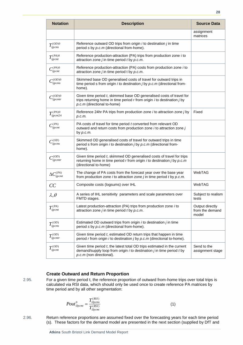
2.94. Table 2.5 provides the notations of variables used for the PA specification (which is arranged according to the appearance of variables in the following text).

Table 2.5 - Notation Used in PA Formulation

Notation Description Source Data

0

IJpcmtPout Given time period t, reference outward from-home trip proportion by p.c.m for origin sector I and destination sector J. These factors are used only once in creating base PA trips.

RSI data

0Pr pcmsret Given time period s, fixed to-home proportion for trips returned in time period r by p.c.m. These factors are only segmented by p.c.m – not enough data is available to populate all ij pairs in a matrix form.

RSI data and NTS data

)(RSI

IJpcmsT The total of from-home trips from 2012 RSI by p.c.m in time period s from origin sector I to destination sector J (directional from-home).

RSI data

)(RSI

IJpcmtT The total of from-home and to-home trips from RSI by p.c.m in time period t from origin sector i to destination sector j (non directional).

RSI data

0)(OD

ijpcmtT Reference OD assignment matrices from origin i to destination j in time period t by p.c.m (non directional).

Calibrated/ validated base

28


Notation Description Source Data

assignment matrices

0)(OD

ijpcmsT Reference outward OD trips from origin i to destination j in time period s by p.c.m (directional from-home).

0)(PA

ijpcmtT Reference production-attraction (PA) trips from production zone i to attraction zone j in time period t by p.c.m.

0)(PA

ijpcmtC Reference production-attraction (PA) costs from production zone i to attraction zone j in time period t by p.c.m.

0)(OD

ijpcmsC Skimmed base OD generalised costs of travel for outward trips in time period s from origin i to destination j by p.c.m (directional from-home).

0)(OD

ijpcmtrC Given time period t, skimmed base OD generalised costs of travel for trips returning home in time period r from origin i to destination j by p.c.m (directional to-home)

0)(

24

PA

ijpcmT Reference 24hr PA trips from production zone i to attraction zone j by p.c.m.

Fixed

)(PA

ijpcmtC PA costs of travel for time period t converted from relevant OD outward and return costs from production zone i to attraction zone j by p.c.m.

)(OD

ijpcmsC Skimmed OD generalised costs of travel for outward trips in time period s from origin i to destination j by p.c.m (directional from-home).

)(OD

ijpcmtrC Given time period t, skimmed OD generalised costs of travel for trips returning home in time period r from origin i to destination j by p.c.m

(directional to-home)

)(PA

ijpcmtC The change of PA costs from the forecast year over the base year from production zone i to attraction zone j in time period t by p.c.m.

WebTAG

CC Composite costs (logsums) over IHL WebTAG

, A series of IHL sensitivity parameters and scale parameters over FMTD stages.

Subject to realism tests

)(PA

ijpcmtT Latest production-attraction (PA) trips from production zone i to attraction zone j in time period t by p.c.m.

Output directly from the demand model

)(OD

ijpcmsT Estimated OD outward trips from origin i to destination j in time period s by p.c.m (directional from-home).

)(OD

ijpcmtrT Given time period t, estimated OD return trips that happen in time period r from origin i to destination j by p.c.m (directional to-home).

)(OD

ijpcmtT Given time period t, the latest total OD trips estimated in the current demand/supply loop from origin i to destination j in time period t by p.c.m (non directional).

Send to the assignment stage

Create Outward and Return Proportion

2.95. For a given time period t, the reference proportion of outward from-home trips over total trips is calculated via RSI data, which should only be used once to create reference PA matrices by time period and by all other segmentation:

)(

)(

0

RSI

IJpcmt

RSI

IJpcms

IJpcmtT

TPout (1)

2.96. Return reference proportions are assumed fixed over the forecasting years for each time period (s). These factors for the demand model are presented in the next section (supplied by DfT and

29


refined locally). For a given time period s, reference proportions for trips returning home in time period r were subject to the following constraint:

1Pr 0 pcmsr

r

et (2)

Create Reference PA Costs and Demands

2.97. For a given time period t, reference demands and costs were calculated by the following two formulae respectively:

00)(0)(0)(

ijpcmt

OD

ijpcmt

OD

ijpcms

PA

ijpcmt PoutTTT (3)

sr

pcmsr

OD

ijpcmtr

OD

ijpcms

PA

ijpcmt etCCC 2/)Pr)'(( 00)(0)(0)( (4)

where sr means that r ranges from the outward from-home time period (s) up to

the last time period (op) in a day, and the ()’ means a transpose. In other words, the

costs defined in (4) are a weighted average of the outward and return legs.

2.98. The daily 24-hour reference demand is the sum of the time period PA demands (which account for only half of total OD demands):

t

PA

ijpcmt

PA

ijpcm TT 0)(0)(

24 (5)

Convert OD Costs to PA

2.99. For each demand/supply loop, the skims from the OD-based assignment by time period (t) were converted to PA costs for feeding into the demand model. With the same formulation as given by (4), the PA costs in forecasting considered both outward and return journeys simultaneously as a weighted sum given below:

sr

pcmsr

OD

ijpcmtr

OD

ijpcms

PA

ijpcmt etCCC 2/)Pr)'(( 0)()()(, (6)

where sr means that r ranges from the outward from-home time period (s) up to

the last time period (op) in a day.

2.100. By adding the relevant return costs, say, any AM tolls will be appropriately allocated to to-home trips occurring in the same and subsequent time periods (i.e. IP, PM and OP), and therefore the impact of AM tolls will be distributed across all time periods rather than incorrectly allocated to the AM demand calculation only.

Incremental Demand Modelling

2.101. For an IHL-based demand modelling, the change of PA costs at the bottom level of hierarchy was simply defined as:

0)()()( PA

ijpcmt

PA

ijpcmt

PA

ijpcmt CCC (7)

2.102. Based on

)(PA

ijpcmtC, the composite costs (i.e. the structured logsums over the various stages of

the demand model) were calculated in the standard way, as presented in the above (para 2.31 – 2.48).

),,,( 0)()( PA

ijpcmt

PA

ijpcmt TCfCC (8)

2.103. Based on the CC and others, the demand model calculates a new set of PA outward-leg

demands for each demand/supply loop, or simply:

30


),,( 0)()( PA

ijpcmt

PA

ijpcmt TCCfT

Convert PA Demands to OD for Assignment

2.104. The outward PA demand )(PA

ijpcmtT output from the demand model was then converted to the OD

form for assignment. The outward from-home OD demands are simply the latest PA demands output from the demand model:

)()( PA

ijpcmt

OD

ijpcms TT (9)

2.105. Return-leg demands were constrained by relevant outward from-home trips that take place in previous time periods. As indicated above, for example, the PM return demands corresponded to proportions of trips travelling out in the AM period, IP period, and PM period respectively.

2.106. For a given time period (t), the formula to calculate to-home demand is given below by applying the fixed return proportions over the latest outward from-home trips:

)'(Pr )(0)(

rs

OD

ijpcmspcmsr

OD

ijpcmtr TetT , (10)

where rs means that s ranges from the first time period (AM) up to the current

time period t.

2.107. Finally, the OD assignment demands were simply the sum of from-home and to-home trips:

)()()( OD

ijpcmtr

OD

ijpcms

OD

ijpcmt TTT (11)

Final Comments

2.108. The demand model calculates the outward estimates of the PA demand directly by the Incremental Hierarchical Logit technique. The return-leg demands were implicitly considered via the outward journeys in the following way:

Return OD costs were incorporated in formulae (4) and (6) above, i.e. the PA

costs are taken as the average OD costs between the outward and return

journeys;

Return-leg trips were calculated by formula (10) from their relevant outward legs

using fixed return proportions. Therefore, any reduction of AM trips resulting

from say, the introduction of AM tolls, would have been mapped onto the

corresponding return legs.

Modelling the Off-Peak Period 2.109. The off-peak (OP) time period (i.e. 19:00 – 07:00) was modelled within the demand model. A

representation of the off-peak costs and demands was needed for the PA-based modelling as defined by the formulae (4) to (11) presented earlier in this section.

2.110. WebTAG does not provide any guidance on how the OP period should be represented. Accordingly, a number of assumptions were made to enable off-peak demand and costs to be estimated for use in the model, reflecting both the limited data available and insignificance of scheme benefits within this period usually. The assumptions were:

OP car users travel at free-flow conditions in the base year;

the change in OP costs was equal to the change in Inter-Peak costs in the same

forecasting year; and

the use of nominal OP base demands was assumed, consisting of 5% of the

corresponding IP base demands.

31


2.111. These assumptions ensured that the switch to the OP period from any of the AM, IP, and PM is always limited and restrictive. For example, the change of OP outward demand was very small in response to the introduction of AM peak tolling (if any). In other words, the introduction of tolling would shift outbound demands to the inter peak period (10:00 -16:00) rather than the off peak period (19:00 to 07:00). The practical limitations of the software and the impact on model runtimes was also an important consideration

Demand and Supply Model Outputs 2.112. The output from the demand model after the sub-mode choice (stage 5) included two sets of

updated matrices for use in the highway and PT assignments namely:

Highway AM peak hour OD matrices (08:00 – 09:00), Inter-Peak average hour

matrices (10:00 – 16:00), and PM peak hour OD matrices (17:00 – 18:00),

segmented by car user class in vehicles and converted to the SBL zoning system;

and

Bus/RT and Rail AM peak hour OD matrices (08:00 – 09:00), Inter-Peak average

hour matrices (10:00 – 16:00), and PM peak hour OD matrices (17:00 – 18:00),

aggregated over person types and journey purposes.

2.113. The output from the PT and Highway assignment models was a set of cost skim matrices, produced by the assignment model to feedback into the demand model, namely:

Highway matrices: skimmed time, distance, and toll matrices; and

Bus/RT and rail matrices: skimmed in-vehicle time, wait time, penalties, and

number of interchanges.

2.114. Both highway and public transport skims were converted from OD format into the equivalent PA format within the demand model consistent with the conversion of PA demand matrices into OD matrices.

2.115. Iterating between the demand and supply models requires the matrices to be converted between the G-BATS3 and SBL zoning systems. As noted above, the SBL zones are simple subdivisions of the G-BATS3 zones.

2.116. To prepare the highway demand matrices for assignment they are expanded to the SBL zoning system using fixed zone conversion factors. After the assignment and skims are carried out (in SBL zoning), the costs in G-BATS3 zoning are calculated for use in the demand model by taking the weighted average over all SBL zone pairs within each G-BATS3 zone pair:

CIJ = ( ij ij ) / ij

where: CIJ is the cost matrix in G-BATS3 zoning dij: is the demand matrix in SBL zoning; and

cij: is the cost matrix in SBL zoning

2.117. A similar process is used in the public transport model, but for practical ease (and so as to not extend run times excessively) intermediate cost skims are done with the SBL version of the public transport network (so that highway travel times can be passed to the public transport model) but with G-BATS3 centroid connectors. This avoids the need to switch between separate EMME databanks with different zoning systems for each demand/supply iteration. For the final public transport assignment, when the sub-mode choice between bus and rapid transit is carried out (see para 2.28), the full SBL public transport model with SBL zoning is used. This requires the public transport demand matrices to be converted from G-BATS3 to SBL zoning, as described above, and transferred to a separate EMME databank in the SBL zoning system.

32


3. Model Parameters and Factors 3.1. This section presents parameters and factors that are used to develop the G-BATS3 demand

model:

VOTs and the introduction of VOT variation with distance;

factors derived from 2009 survey data, including segmentation factors, PA

pseudo-tour factors, occupancies and others; and

bus and rail fares.

Value of Time (VOT) Variation with Distance

3.2. Table 3.1 presents the base year 2012 VOT parameters by person for demand modelling, based on the values given in WebTAG Unit 3.5.6.

Table 3.1 - 2012 Value of Time by Person-Type

Demand Segment Purpose Value of Time

(pence / minute)

Car Available Commuting (HBW) <£17,500 8.97

Commuting (HBW) £17,500 - £35,000 8.97

Commuting (HBW) >£35,000 8.97

Other (HBO+NHBO) <£17,500 7.94

Other (HBO+NHBO) £17,500 - £35,000 7.94

Other (HBO+NHBO) >£35,000 7.94

Work (HBEB+NHBEB) 36.96

Non-Car Available Commuting (HBW) 4.49

Other (HBO+NHBO) 3.97

Work (HBEB+NHBEB) 18.48

3.3. Table 3.2 below presents a summary of the VOTs used in the demand model for the CA HBO and NHBO and NCA HBO, NHBO and HBW trip purposes, where the VOT variation by distance was applied (see section on Cost Damping above for further details). The table shows the average value of VOT (i.e. as given in Table 3.1) as well as the matrix average, minimum and maximum.

Table 3.2 - Variation of VOT with Distance

Purpose Car Available (HBO/NHBO) Non Car Available

Income Low

Income median

Income High

HBW HBO/NHBO

Average Value 7.94 7.94 7.94 4.49 3.97

Matrix Average 9.47 9.47 9.47 5.83 4.73

Matrix Minimum 5.60 5.60 5.60 2.81 2.80

Matrix maximum 30.06 30.06 30.06 26.73 15.03

3.4. It is noted that the VOT variation by distance has been applied to all non-work purposes for non-car available users, but only to the HBO and NHBO demand segments for car available users.

33


Initially, the variation was also applied to the CA HBW demand segment but the outturn elasticities appeared too low in realism tests. After discussions with the Department, the central VOT values were applied to the CA HBW segment.

3.5. It is also noteworthy that the variation of VOT with distance is applied only to the demand model, and not to the assignment models.

Factors Derived from Survey Data 3.6. The development of the demand model involved the derivation of local factors, such as demand

segmentation factors, PA returning factors, and car occupancy factors.

3.7. One of the principal data sources for the demand model was the 2012 RSI survey data, supplemented by other data sources such as TEMPRO and the National Travel Survey where necessary. The 2012 RSI surveys were undertaken to collect up-to-date travel patterns to strengthen existing demand matrices. Altogether, 5 sites were surveyed in the South Bristol area during March 2012.

3.8. The following factors were derived from the 2012 RSI survey data:

Household income band factors;

Purpose splitting factors; and

Car occupancy factors by purpose, household income band, and time period.

3.9. For car, purpose split factors were derived from the 2012 RSI surveys on a sector-sector basis. Table 3.3 below provides the average factors by purpose and time period for the base year 2012. Within each purpose, car demand was split into equal income segments.

Table 3.3 - Demand Segmentation Factors by Purpose (Car)

Purpose AM IP PM

HBO 0.156 0.423 0.289

NHBO 0.045 0.16 0.252

NHBEB 0.038 0.151 0.087

HBEB 0.022 0.019 0.016

HBW 0.74 0.247 0.355

Total 1.00 1.00 1.00

3.10. For bus, purpose split factors were derived from the 2009 bus origin-destination surveys on a

sector-sector basis. The average bus segmentation factors by purpose are given in Table 3.4 below. Within each purpose, bus demand was split into equal income segments

Table 3.4 - Average Bus Purpose Split Factors

Demand Segment AM IP PM

HBO 0.27 0.91 0.20

NHBO 0.10 0.30 0.07

NHBEB 0.01 0.02 0.01

HBEB 0.02 0.01 0.02

HBW 0.60 0.42 0.44

3.11. Table 3.5 gives highway car occupancy factors for the base year 2012 by purpose, and by time

period. Note that no distinction was made between home-based and non home-based trips within a purpose.

34


Table 3.5 - Car Occupancy Factors

Time Period / Segment Commuting Work Other

AM Peak

< £17,500 1.18 Not Applicable 1.48

£17,500 - £35,000 1.18 1.48

> £35,000 1.18 1.48

Average 1.18 1.30 1.48

Inter-Peak

< £17,500 1.19 Not Applicable 1.58

£17, 500 - £35,000 1.19 1.58

> £35,000 1.19 1.58

Average 1.19 1.13 1.58

PM-Peak

< £17,500 1.20 Not Applicable 1.58

£17, 500 - £35,000 1.20 1.58

> £35,000 1.20 1.58

Average 1.20 1.00 1.58

3.12. Table 3.6 summarises the 2012 from-home / to-home factors derived from the 2006 RSI

surveys. These base year values are assumed to be constant across all the forecast years.

Table 3.6 - From-home / To-home Factors


HBW <£17,500 0.96 / 0.04 0.55 / 0.45 0.12 / 0.88

HBW £17,500 - £35,000 0.96 / 0.04 0.55 / 0.45 0.12 / 0.88

HBW >£35,000 0.96 / 0.04 0.55 / 0.45 0.12 / 0.88

HBO <£17,500 0.86 / 0.14 0.65 / 0.35 0.55 / 0.45

HBO £17,500 - £35,000 0.86 / 0.14 0.65 / 0.35 0.55 / 0.45

HBO >£35,000 0.86 / 0.14 0.65 / 0.35 0.55 / 0.45

HBEB 0.97 / 0.03 0.54 / 0.46 0.22 / 0.78

3.13. The factors to convert demand from the peak hour to peak period (or inverse for the reverse),

derived from the 2012 RSI surveys, are presented below in Table 3.7 by time period, purpose and mode.

35


Table 3.7 - Peak Hour to Peak Period Factors


Car

Commuting (HBW) 2.78 6.00 2.58

Other (HBO+NHBO) 3.07 6.00 2.91

Work (HBEB+NHBEB) 2.74 6.00 3.43

Bus

All Purposes 2.40 6.00 2.80

Rail

All Purposes 2.70 6.00 2.10

3.14. Local household survey data was not available and the car availability person type factors were

derived for the PT segmentation using the 2006 Avon Rail Surveys and the 2009 Bus origin-destination surveys for bus and rail respectively. Table 3.8 presents the Car-available (CA) and non-Car available (NCA) splitting factors for rail and bus users in the 2012 base year.

Table 3.8 - CA / NCA Splits for Rail & Bus Users


Rail CA / NCA 0.651 / 0.349 0.559 / 0.441 0.716 / 0.284

Bus CA / NCA 0.265 / 0.735 0.25 / 0.75 0.285 / 0.715

Fixed Returning Proportions 3.15. Table 3.9a and b present the returning proportions used in the demand model for the three

home-based purposes. The DfT supplied national tour information derived from NTS datasets from which returning proportions were derived. The national average values were subsequently adjusted to reflect the travel demand in the sub-region. To ensure consistency with the calibrated base year supply models, a substantial volume of analytical work was undertaken to ensure consistency between the base year validated matrices and the outward/return proportions.

Table 3.9a - Highway Fixed Returning Proportions

HBW HBO HBEB

AM Outward

AM Return 0.03 0.27 0.07

IP Return 0.24 0.56 0.38

PM Return 0.65 0.15 0.44

OP Return 0.08 0.01 0.11

Total 1.00 1.00 1.00

IP Outward

IP Return 0.26 0.72 0.50

PM Return 0.51 0.24 0.38

OP Return 0.23 0.04 0.12

Total 1.00 1.00 1.00

36


HBW HBO HBEB

PM Outward

PM Return 0.46 0.58 0.40

OP Return 0.54 0.42 0.60

Total 1.00 1.00 1.00

OP Outward

OP Return 1.00 1.00 1.00

Total 1.00 1.00 1.00

Table 3.10b - PT Fixed Returning Proportions

Bus

Rail

HBW HBO HBEB HBW HBO HBEB

AM Outward

AM Return 0.04 0.22 0.12 0.04 0.25 0.09

IP Return 0.35 0.59 0.38 0.13 0.62 0.35

PM Return 0.54 0.18 0.31 0.75 0.12 0.42

OP Return 0.08 0.01 0.19 0.08 0.01 0.15

Total 1.00 1.00 1.00 1.00 1.00 1.00

IP Outward

IP Return 0.30 0.72 0.64 0.25 0.79 0.56

PM Return 0.44 0.25 0.21 0.53 0.17 0.31

OP Return 0.26 0.03 0.15 0.22 0.04 0.13

Total 1.00 1.00 1.00 1.00 1.00 1.00

PM Outward

PM Return 0.46 0.59 0.40 0.47 0.58 0.40

OP Return 0.54 0.41 0.60 0.53 0.42 0.60

Total 1.00 1.00 1.00 1.00 1.00 1.00

OP Outward

OP Return 1.00 1.00 1.00 1.00 1.00 1.00

Total 1.00 1.00 1.00 1.00 1.00 1.00

Base Year Bus and Rail Fares 3.16. Public transport fares are excluded from the EMME assignment module and were incorporated

into PT generalised cost calculations within the demand model.

3.17. The bus fares matrix was derived from published fare data. Further details are given in the PTAM Development Report.

3.18. Rail fares are calculated based on the function of skimmed rail OD distances and connected bus interchanges:

AM / PM fare = (0.4+0.09583*Distance_km) + 1.08* number of bus boardings

IP fare = (0.4+ 0.07403 *Distance_km) + 1.08* number of bus boardings

37


3.19. Bus and rail fares were uplifted from 2006 to 2012 values using the factors shown in Table 3.10.

3.20. Rail crowding is not modelled.

Table 3.11 - Uplift Factors for PT Fares

Mode 2006 to 2012 Uplift Factor Source

Bus 9% Comparison of a selection of ticket prices within the WoE area

Rail 21% Office of the Rail Regulator Rail Fares Index

38


4. Demand Model Validation

Introduction 4.1. The validity of the demand model has been assessed by realism tests undertaken rigorously.

The main purpose of the realism tests is to demonstrate that the chosen model parameters (either locally calibrated or adopted from the nationally recommended parameters) replicate long-term elasticities derived from empirical observations and/or best practice.

4.2. The target elasticities for the realism tests, as defined by WebTAG Unit 3.10.4, are:

Car fuel cost - recommended elasticity between -0.1 to -0.4, with an overall target

value of -0.25 to -0.35 across all segments;

Car journey time - recommended elasticity less than -2.00; and

PT fare - recommended elasticity between -0.2 to -0.9.

4.3. WebTAG recommends the use of locally calibrated demand parameters if they are available from Revealed Preference and Stated Preference data. If these are not available, as is the case with G-BATS3, WebTAG recommends the use of illustrative sensitivity parameters provided in WebTAG Unit 3.10.3. In either case, the robustness of the demand model validation needs to be demonstrated through the application of a set of realism tests.

4.4. The demand model has introduced value of time variation with trip distance for consumer trips as explained previously in Section 3.

4.5. This section presents the demand model elasticities derived from the realism tests, by using the sensitivity parameters and structure parameters presented in Section 3, together with the introduction of VOT variation with distance for non-Work trips.

Convergence Between Supply-Demand 4.6. The five-stage demand model employs an iterative method to achieve convergence between

the assignment models (i.e. SATURN highway and EMME PT) and the EMME-coded demand model. Convergence was achieved by passing costs from the assignment models to the demand model and subsequently passing trips from the five-stage demand model back to the assignment models; the process terminated once the convergence criterion had been met.

4.7. Two convergence algorithms were implemented to create a stable converged solution between the cycling of demand and supply responses. The convergence algorithms were:

the method of successive average (MSA); and

the average method which simply used the mean value between previous results

and the current new estimates.

4.8. The testing work undertaken identified that the simple average method provided a more stable (and quicker) solution and this was adopted for the modelling system.

4.9. The recommended criterion by WebTAG Unit 3.10.4, for measuring convergence between demand and supply models, is the demand/supply gap over all segments as defined by:

where:

Xijctm is the current flow vector or matrix from the model

39


C(Xijctm) is the generalised cost vector or matrix obtained by assigning that

matrix

D(C(Xijctm)) is the flow vector or matrix output by the demand model, using the

costs C(Xijctm) as input

ijctm represents origin i, destination j, demand segment/user class c, time period

t and mode m.

4.10. It is important to achieve a high level of supply-demand convergence. WebTAG suggests that the convergence level, measured by %GAP, should be lower than 0.2% (or, if that cannot be achieved, a more relaxed criterion related to the projected benefits of a scheme). Table 4.1 gives an example of the %GAP values to show the convergence of the demand model in realism tests.

Table 4.1 - Example of Convergence for Realism Tests

Demand/Supply Iteration %GAP

1 38.1003

2 24.6568

3 14.4695

4 7.9964

5 4.2826

6 2.2666

7 1.2006

8 0.6501

9 0.3760

10 0.2185

11 0.1590

Realism Tests 4.11. The realism tests undertaken identified a set of sensitivity parameters which were the most

appropriate for the sub-region (with respect to the demand hierarchy form presented in Figure 2.2). The demand response parameters presented later in this chapter were the result of testing the range of illustrative parameters in WebTAG via an iterative process of tuning.

4.12. The arc elasticity formulation recommended by WebTAG was used for the realism testing for a 10% increase in cost:

,)1.1log(

)log()log(

)log()log(

)log()log( 01

01

01 TT

CC

TTe

where the superscripts 0 and 1 indicate values before and after the change in cost

respectively, and for:

Car fuel cost elasticity: T represents the car-kms travelled whilst C represents

fuel costs;

PT fare elasticity: T represents PT trips and C represents fares.

4.13. The realism tests were undertaken assuming:

a 10% increase in fuel prices for the car fuel cost elasticity test; and

a 10% increase in bus and rail fares for the public transport fare elasticity test.

40


Car Fuel Cost Elasticities

Network Based

4.14. The Car fuel cost elasticities in terms of car vehicle kilometres with respect to (w.r.t) fuel costs, are shown below in Table 4.2, presented by segmentation of highway assignment user classes, i.e. by household income and by purpose work/non-work. Note that it was not possible to separately calculate the elasticities for “commuting” and “other” purposes (nor the non-work categories) at network level as they were combined together for assignment purposes.

4.15. The network-based fuel cost elasticities in Table 4.2 are given for each of the three peak hours. Table 4.2 also distinguishes between the various network areas (i.e. simulation, buffer link and buffer centroid connectors). The simulation area covers the entire built-up area of Bristol. The elasticity values presented are obtained by direct calculation using SATURN output network statistics.

4.16. Table 4.2 demonstrates a pattern of fuel cost elasticities by user class or household income consistent with the equal split between the income bands.

Table 4.2 – G-BATS3 SBL Car Fuel Cost Elasticity (WebTAG: -0.25 to -0.35)

PCU-Kms w.r.t Fuel Cost AM IP PM Annual

UC1 Car – Non Work IL

Simulation Area -0.26 -0.26 -0.21 -0.25

Buffer Area (B) -0.24 -0.17 -0.19 -0.19

Buffer Area (BCC) -0.24 -0.18 -0.23 -0.20

Total -0.25 -0.20 -0.21 -0.21

UC2 Car – Non Work IM

Simulation Area -0.26 -0.26 -0.17 -0.24

Buffer Area (B) -0.24 -0.17 -0.07 -0.16

Buffer Area (BCC) -0.24 -0.18 -0.04 -0.16

Total -0.25 -0.20 -0.09 -0.18

UC3 Car – Non Work IH

Simulation Area -0.26 -0.26 -0.21 -0.25

Buffer Area (B) -0.24 -0.17 -0.19 -0.19

Buffer Area (BCC) -0.24 -0.18 -0.23 -0.20

Total -0.25 -0.20 -0.21 -0.21

Car – Total Non Work

Simulation Area -0.26 -0.26 -0.20 -0.24

Buffer Area (B) -0.24 -0.17 -0.15 -0.18

Buffer Area (BCC) -0.24 -0.18 -0.17 -0.19

Total -0.25 -0.20 -0.17 -0.20

UC4 Car - Work

Simulation Area -0.04 -0.08 -0.01 -0.06

Buffer Area (B) -0.04 -0.06 -0.08 -0.06

Buffer Area (BCC) -0.05 -0.06 -0.11 -0.07

Total -0.04 -0.07 -0.07 -0.06

41


PCU-Kms w.r.t Fuel Cost AM IP PM Annual

Total Cars

Simulation Area -0.23 -0.23 -0.19 -0.22

Buffer Area (B) -0.22 -0.15 -0.14 -0.16

Buffer Area (BCC) -0.22 -0.15 -0.16 -0.17

Total -0.22 -0.17 -0.16 -0.18

4.17. These elasticities are on the lower side of the range and have been affected by fixed elements within the matrix (external to external trips).

Matrix Level

4.18. The matrix-based vehicle-km fuel cost elasticities are presented below in Table 4.3 with the elasticities reported by time period, by ‘super’ sector (i.e. Internal or External), and by purpose (i.e. HBW / HBO / NHBO / Work). Figure 4.1 shows the four geographical sectors making up the ‘Internal’ super sector (i.e. sectors 1 to 4 representing Bristol Central / Inner / Outer, and Greater Bristol) and the ‘External’ super sector (i.e. sector 5).

Figure 4.1 - Five Sector Reporting System

4.19. It is noted that the demand model does not consider the impact on external to external trips. Table 4.3 includes internal to internal demand and internal to external demand (I to I&E) only. (E-E trips are inelastic in the demand models which lead to E-I demands being only partially modelled and thus they are also excluded from the analysis).

4.20. The car vehicle-kilometre elasticities shown in Table 4.3 demonstrate that the demand model replicates published elasticities of vehicle-kilometres with respect to fuel cost. The overall average fuel cost elasticity is -0.32, which is in the middle of the range of -0.25 to -0.35 recommended by WebTAG.

42


Table 4.3 – Matrix-Based Car Fuel Cost Elasticity

Time Period

Movement Type

HBW HBO NHBO Non-Work (Total)

Work All

AM I to I&E -0.36 -0.50 -0.42 -0.42 -0.11 -0.39

IP I to I&E -0.24 -0.34 -0.36 -0.32 -0.14 -0.29

PM I to I&E -0.23 -0.44 -0.37 -0.33 -0.11 -0.31

ALL DAY I to I&E -0.28 -0.40 -0.38 -0.35 -0.13 -0.32

4.21. Looking at the matrix-based values by purpose, Table 4.3 shows that the all day elasticities are

generally within the recommended range -0.25 to -0.35 for all purposes. As would be expected:

Discretionary trips such as HBO and NHBO trips exhibit higher elasticities than

more obligatory HBW trips which are doubly-constrained;

Work trips exhibit the lowest elasticities as they have the highest values of time;

and

.cost damping and other sensitivity parameters will also have affected these

results.

4.22. Table 4.3 shows that the fuel cost elasticity is greatest in the AM Peak, followed by the Inter-peak, with the PM Peak being the slightly higher than the Inter-peak. The conventional view drawn from experience of models developed suggests that it is travel in the IP which is expected to most sensitive to changes in fuel costs, primarily because of a higher proportion of discretionary travel in the Inter-peak period.

4.23. However, it is reasonable to expect the pattern by time period to be different for G-BATS3 due to the particular PA formulation used (as illustrated in Table 3.9), where the return leg of home-based trips is allocated to a time period based on fixed proportions, and trips travelling outbound in the Inter-peak and PM peak are assumed not to return earlier in the day. The return leg allocation is not therefore sensitive to changes in cost as it is effectively fixed by the choice of outbound time period.

4.24. In the AM Peak, the vast majority of home-based trips are on the outbound leg, whereas in the Inter-peak the outbound and return proportions are approximately equal, and in the PM Peak almost all the trips are returning home. This means that the AM Peak can reasonably be expected to be most sensitive, followed by the Inter-peak, as shown in the pattern of fuel elasticities by time period.

4.25. Table 4.4 shows a range of indicators of the relative strength of car fuel cost elasticity for the Bristol area. The picture is mixed, with some indicators suggesting a weaker elasticity and others a stronger elasticity. It therefore considered appropriate for the fuel cost elasticity to be in the middle of the acceptable range at -0.32.

Table 4.4 – Indicators for Strength of Car Fuel Cost Elasticity

Indicator Bristol National Average

Likely Effect on Elasticity

AM IP PM All

Car occupant mode share 88% 91% 90% n/a 84% Weaker

Car driver mode share 70% 64% 65% n/a 54%

Average trip length (km) n/a n/a n/a 22.0 13.6 Stronger

Proportion of Work trips 11% 19% 5% n/a 5.2% Weaker

Gross weekly pay (£) n/a n/a n/a 479.8 491.0 Neutral

Sources: National Travel Survey 2008, G-BATS3 SBL Model, Nomis Official Labour Market Statistics, Earnings by residence (2009)

4.26. The above tables and analysis demonstrate that the G-BATS3 demand model is a robust tool for forecasting highway demand in scheme tests.

43


Journey Time Elasticities

4.27. The journey time elasticities derived from the realism tests should reflect the TAG values of less than -2.00 and are presented below in Table 4.5; which shows that journey time elasticities were all less than -2.00 as recommended by WebTAG. The overall journey time elasticities for the three time periods are-0.69, -0.55, and -0.55, for AM Peak, Inter-peak and PM Peak respectively, and the total journey time elasticity all day is –0.56.

Table 4.5 - Matrix-based Journey Time Elasticities

Time Period

Movement Type


Work All

AM I to I&E -0.61 -0.86 -0.73 -0.73 -0.37 -0.69

IP I to I&E -0.43 -0.61 -0.64 -0.58 -0.43 -0.55

PM I to I&E -0.40 -0.77 -0.65 -0.58 -0.31 -0.55

ALL DAY I to I&E -0.43 -0.66 -0.65 -0.59 -0.41 -0.56

Public Transport Fare Elasticities

4.28. Fare elasticities derived from PT realism tests should reflect WebTAG values between -0.2 and -0.9. Matrix-based PT fare elasticities are presented below in Table 4.6 for “I to I&E” movements only, (as with the case exhibited for car fuel cost elasticities).

4.29. The PT fare elasticities presented below are evaluated as the change of the total number of public transport trips (including all PT sub modes) with respect to the 10% increase of bus and rail fare. No concession fare is considered in the G-BATS3 modelling framework.

4.30. Table 4.6 is arranged by purpose, time period and person type CA and NCA. It shows that the total PT fare elasticity is -0.52 across all segments for car available users and -0.55 and -0.17 for the Non-Work purposes and Work purpose, respectively.

4.31. Table 4.6 shows that the discretionary NHBO trip purpose exhibits the highest elasticities. WebTAG notes that there is little or no empirical evidence for the pattern of elasticities by trip purpose, and there is thus no benchmark for comparison.

Table 4.6 – Matrix-based PT Fare Elasticities

Time Period

Movement Type


Work All

Car Available

AM I to I&E -0.47 -0.60 -0.89 -0.54 -0.15 -0.50

IP I to I&E -0.52 -0.64 -0.87 -0.65 -0.25 -0.63

PM I to I&E -0.31 -0.53 -0.79 -0.41 -0.08 -0.39

All Day I to I&E -0.42 -0.62 -0.85 -0.55 -0.17 -0.52

Non-Car Available

AM I to I&E 0.07 -0.28 -0.27 -0.07 -0.36 -0.09

IP I to I&E 0.00 -0.10 -0.11 -0.07 0.01 -0.07

PM I to I&E 0.17 -0.10 -0.21 0.03 0.18 0.03

All Day I to I&E 0.08 -0.13 -0.16 -0.05 -0.11 -0.05

4.32. It is worth mentioning that since PT assignments are modelled with the Emme software which is not capable of incorporating stage-based bus and rail fare in route choice modelling (this applies to most PT modelling software). Therefore, the PT fare is considered in the demand model only and thus may have influence in the fare elasticity patterns presented.

44


4.33. Non-car available (NCA) PT demands are captive to PT and their fare elasticities are presented in the bottom part of Table 4.6. It shows that the NCA fare elasticities are considerably smaller than their counterparts with CA users, reflecting that there is very limited choice available for this type of PT user.

4.34. NCA HBW elasticities in Table 4.6 are shown to be slightly positive for I to I&E movements. These trip purposes have a very limited set of responses available because they are captive to PT, and trip frequency effects are not modelled. Further, in order to satisfy the double constraints for HBW, external-to-internal (E-I) movements need to be included also. When considering all movements together (“I to I&E” and “E-I”), the NCA the total elasticity overall is -0.07. These elasticities indicate that increasing the PT fare cost by 10% has virtually no impact on the NCA segments, as users have no alternatives but PT.

Sensitivity Parameters from Realism Tests 4.35. By importing values from WebTAG Unit 3.10.3, demand modelling sensitivity parameters given

below were derived from the realism tests presented in the above.

Destination Choice

4.36. Highway destination choice sensitivity parameters for G-BATS3 are presented below in Table 4.7 (ignoring the negative signs). WebTAG illustrative values are shown along with lambda parameters used in the demand model. Highway destination choice sensitivity parameters adopted for G-BATS3 are all within +/- 25% of the WebTAG median values

Table 4.7 - Destination Choice Parameters (Highway)

Purpose HIGHWAY

WebTAG (Minimum/Median/Maximum) SBL

HBO 0.074/0.090/0.160 0.113

NHBO 0.073/0.077/0.105 0.077

NHBEB 0.069/0.081/0.107 0.069

HBEB 0.038/0.067/0.106 0.050

HBW 0.054/0.065/0.113 0.054

4.37. The PT destination choice sensitivity parameters for G-BATS3 are presented below in Table 4.8 (ignoring the negative signs also as highway). Again, WebTAG illustrative values are shown along with lambda parameters used in the demand model. PT destination choice sensitivity parameters adopted for G-BATS3 are all within +/- 25% of the WebTAG median values.

4.38. Note that for PT demand modelling, as recommended by WebTAG, the same sensitivity parameters were used for both Car Available (CA) and Non-Car Available (NCA) person types.

Table 4.8 - Destination Choice Parameters (PT)

Purpose Public Transport

WebTAG (Minimum/Median/Maximum) SBL

HBO 0.033/0.036/0.062 0.036

NHBO 0.032/0.033/0.035 0.033

NHBEB 0.038/0.042/0.045 0.045

HBEB 0.030/0.036/0.044 0.044

HBW 0.023/0.033/0.043 0.033

45


Main Mode Choice

4.39. The tree structure parameters for the main mode choice are given in Table 4.9 below, together with the range of illustrated scale parameters specified in Unit 3.10.3. Clearly, they are all lie within the recommended ranges, more accurately, they all are set as WebTAG median thetas exactly by purpose (during the realism tests, the theta values were fixed as such that only lambda parameters for destination choices were allowed to vary).

Table 4.9 - Main Mode / Time Period Choice Parameters

Purpose WebTAG Theta (Minimum/Median/Maximum)

Demand Model Theta

HBO 0.27/0.53/1.00 0.53

NHBO 0.62/0.81/1.00 0.81

NHBEB 0.73/0.73/0.73 0.73

HBEB 0.26/0.45/0.65 0.45

HBW 0.50/0.68/0.83 0.68

4.40. Note that WebTAG suggested the main mode choice and time period choice should be considered simultaneously; therefore, the same theta values are used for the time period choice and main mode choice inside the G-BATS3.

4.41. Realism test results presented earlier in this Chapter show that the above parameters lead to satisfactory elasticities, when Value of Time (VOT) variation with distance has been introduced for the HBO and NHBO trip purposes as described in Chapter 3.

46


5. Summary

5.1. The G-BATS3 demand model was developed to assess the transport impacts of a range of potential transport interventions in the West of England sub-region. These potential interventions include demand management schemes as well as Major Scheme Bids.

5.2. The demand model is a five-stage multi-modal incremental model that considers the impact on frequency choice, main mode choice, time period choice, destination choice, and sub mode choice in response to changes in generalised costs for highway and public transport.

5.3. The demand model represents travel demand over a 24-hour period. It is a Production-Attraction (PA) based model with explicit time period choice modelling based on the use of fixed return proportions derived from national average values obtained from DfT NTEM/TEMPRO datasets.

5.4. The G-BATS3 demand model follows the latest WebTAG guidance and functions at a slightly more aggregate zoning level (600 zones) than that of the SBL highway model composed of 650 zones. The assignment model zones are sub-divisions of demand model zones, ensuring that the consistency between costs and demand at each stage of the G-BATS3 SBL model is maintained appropriately.

5.5. The demand model iterates between the hourly-based AM, IP and PM supply models and the 24-hour demand model. Two convergence algorithms were implemented, namely the MSA algorithm and the average algorithm to achieve convergence in the demand/supply interactions with the latter selected based on its performance following testing. The demand model achieves the required levels of convergence stipulated by WebTAG.

5.6. VOT variation with trip length has been introduced into the demand model for car available HBO and NHBO trips, and non car available non-work purposes including HBW. This technique has helped in achieving WebTAG required elasticities especially for longer distance trips due to the nature of the logit-based demand modelling framework.

5.7. The theta parameters and highway/PT lambda parameters adopted are mostly within +/-25% of WebTAG illustrative values. The realism tests undertaken have successfully identified a set of demand response parameters that replicated both the local conditions and conformed to the hierarchical tree structure recommended by WebTAG, that is, FMTD (Frequency, Mode, Time period, and Destination choice).

5.8. The derived car fuel elasticity, car journey time elasticity and PT fare elasticity, established through the realism tests, have been reported by purpose, time period and spatial locations. All outturn elasticity values by purpose are within WebTAG required ranges. The overall fuel cost and PT fare elasticities are -0.32 and -0.55 respectively – both within the range of WebTAG target values. The realism tests showed that, as expected, discretionary trips (HBO/NHBO) exhibited higher fuel cost elasticities than non-discretionary trips (HBW/EB).

5.9. The pattern of elasticities by time period shows that the AM Peak period is most sensitive, followed by the inter-peak period for fuel cost elasticity. This is explained by the particular PA formulation used for G-BATS3, whereby the time period allocation for the return leg of home-based trips is based on fixed proportions, and hence the Inter-peak and PM Peak periods are more restricted than the AM Peak period.

5.10. On this basis, the G-BATS3 SBL demand model is considered to be ‘fit for purpose’ as described in Chapter 1.

Contact name: Graham Bown Address: Sir William Atkins House Ashley Avenue Epsom Surrey KT18 5AL Email: [email protected] Telephone: 01372 756899

© Atkins Ltd except where stated otherwise. The Atkins logo, ‘Carbon Critical Design’ and the strapline ‘Plan Design Enable’ are trademarks of Atkins Ltd.

mailto:[email protected]

south bristol link demand model report - amazon s3 · atkins south bristol link demand model report...

Documents