s.p. novikov - math 740
TRANSCRIPT
S.P. Novikov - MATH 740
Spring 2014
S. Novikov - office 3112 (MATH)e-mails: [email protected] , [email protected] hours: MONDAY, WEDNESDAY, FRIDAY 16-17 pm
Contents
Lecture 1. Introduction: Textbooks and General Remarks.Local coordinates: What is Cartesian system of coordinates.Examples. 5
Lecture 2. Manifolds and Atlases. 7
Lecture 3. C∞-manifolds, Atlases, Charts. Especially goodAtlases. Implicit functions and Inversion. Imbedding ofCompact Manifolds in RN . Immersions. 11
Lecture 4. Manifolds and Submanifolds: Implicit functionsand Inversion. Vectors and Covectors. 17
Homework 1. 21
Lecture 5. Manifolds and vectors fields. Important Exam-ples. 22
Lecture 6. Group Manifolds. Lie Algebra. Important Ex-amples. 25
Lecture 7. Group Manifolds: Compact Lie groups. Most im-portant Examples. Noncompact Lie groups. Most importantExamples. Lie Algebras. Gradient-like Systems. 29
1

Homework 2. 34
Lecture 8. Riemannian, Pseudo-Riemannian and Symplec-tic Geometries.Complex Geometry. Restriction of Metric tosubmanifolds. Length of curves and Fermat Principle. 34
Lecture 9. Geodesics and Calculus of variations. Length andAction functionals. Examples. 39
Lecture 10. Variational problem and geodesics on Rieman-nian manifolds: Action Functional, Lagrangian, Energy, Mo-mentum. Conservation of Energy and Momentum. 44
Homework 3. 49
Lecture 11. Geodesics and Action Functional. Examples.Hamiltonian form of Euler - Lagrange equation. Conserva-tion of Energy and Momentum. Euclidean, Spherical andHyperbolic Geometries. 50
Lecture 12. Curvature of curves and surfaces. How to dif-ferentiate tangent vector fields? 54
Lecture 13. Vector bundles. Connection and Curvature.Parallel transport. 60
Homework 4. 63
Lecture 14. Vector bundles. Connection and Curvature.Parallel transport. 65
Lecture 15. Connections in tangent bundle. Curvature.Ricci curvature. Einstein equation. Spaces of constant cur-vature. 68
Appendix to Lecture 15. . . . . . . . . . . . . . . . . . . . . . 71
Lecture 16. Tensor fields. Curvature as a tensor field. Gaus-sian curvature for surfaces in R3 . 71
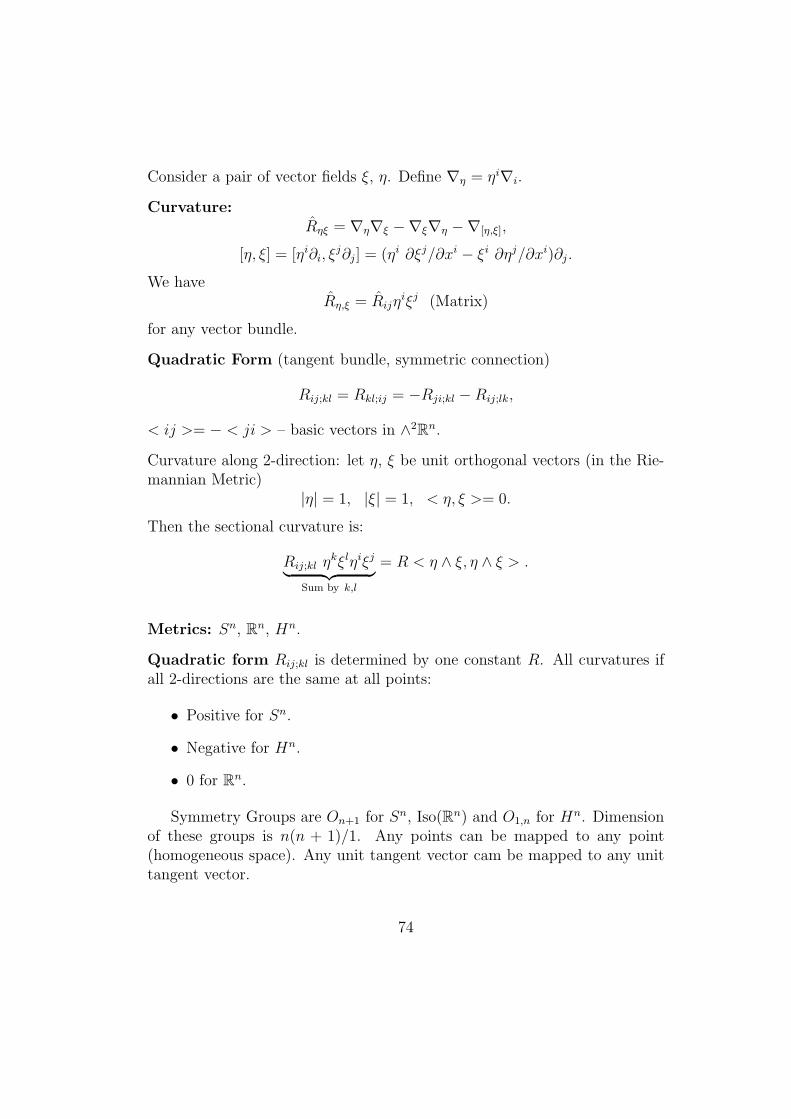
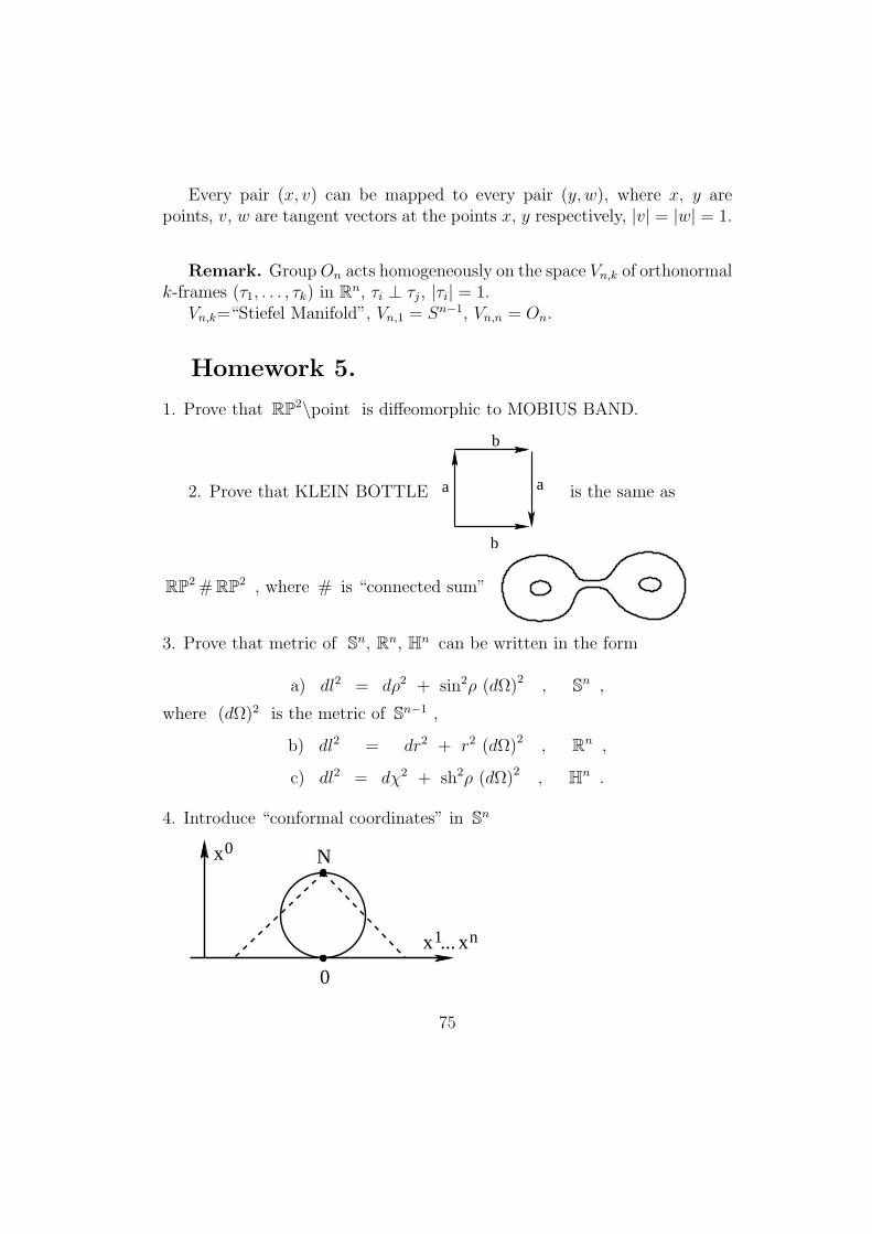
Homework 5. 75
2
Homeworks 2, 3, 4. Solutions. 76Homework 2. Solutions. . . . . . . . . . . . . . . . . . . . . . 76Homework 3. Solutions. . . . . . . . . . . . . . . . . . . . . . 78Homework 4. Solutions. . . . . . . . . . . . . . . . . . . . . . 80
Lecture 17. Differential forms. 81
Homework 5. Solutions. 84
Lecture 18. Differential forms. De Rham operator. 85
Lecture 19. Differential forms. Cohomology. 90
Homework 6. 94
Lecture 20. Differential forms and tensors. Categorial prop-erties. Cohomology and Stocks formula. Homotopy invari-ance of Cohomology. 95
Lecture 21. Homotopy invariance of Cohomology. Examplesof differential forms. Symplectic and Kahler manifolds. 99
Lecture 22. Symplectic Manifolds and Hamiltonian Systems.Poisson brackets. Preservation of Symplectic form by Hamil-tonian System. 103
Homework 7. 106
Lecture 23. Volume element in Compact Lie groups. Av-eraging of differential forms and Riemannian Metric. Coho-mology of Homogeneous Spaces. 107
Lecture 24. Volume element in Compact Lie groups. Av-eraging of differential forms and Riemannian Metric. Coho-mology of Homogeneous Spaces. 111
Lecture 25. Approximation and Transversality. 113
Homework 8. 117
3
Homework 6 and Homework 7. Solutions. 118Homework 6. Solutions. . . . . . . . . . . . . . . . . . . . . . 118Homework 7. Solutions. . . . . . . . . . . . . . . . . . . . . . 119
Lecture 26. Transversality. Imbeddings and Immersions ofManifolds in Euclidean Spaces. 122
Lecture 27. Intersection Index and Degree of Map. 124
Lecture 28. Intersection Index and Degree of Map. 128
Homework 9. 131
Lecture 29. Intersection Index and Degree of Map. 131
Lecture 30. Two applications of differential forms: Degreeof Map and Hopf Invariant. 136
Lecture 31. Comparison of notations of our Lectures withbook of Do Carmo “Riemannian Geometry”. 140
Homework 10. 144
Homeworks 8, 9. Solutions. 145Homework 8. Solutions. . . . . . . . . . . . . . . . . . . . . . 145Homework 9. Solutions. . . . . . . . . . . . . . . . . . . . . . 148
Lecture 32. Geodesics. Gauss Lemma. 150
Lecture 33. Local minimality of geodesics. 154
Homework 11. 156
Lecture 34. Riemannian Curvature. Examples. 157
Homeworks 10, 11. Solutions. 160Homework 10. Solutions. . . . . . . . . . . . . . . . . . . . . . 160Homework 11. Solutions. . . . . . . . . . . . . . . . . . . . . . 162
4
Lecture 1. Introduction: Textbooks and Gen-
eral Remarks. Local coordinates: What is
Cartesian system of coordinates. Examples.
Textbooks:Manfredo P. do Carmo. Riemannian Geometry.Victor Guillemin, Alan Pollack. Differential Topology.
Additional Literature:J. Milnor. Morse Theory.S.P. Novikov, I.A. Taimanov. Modern Geometric Structures And Fields.B.A. Dubrovin, A.T. Fomenko, S.P. Novikov. Modern Geometry - Methodsand Applications: Parts I, II.
Differential Manifolds, definition, maps, submanifolds.Language of general topology is necessary: spaces, continuous maps,homeomorphisms, compactness, metric and Hausdorff spaces.Basic Tools from multivariable calculus: Implicit Functions, Approxi-mations and Transversality. Theorems will be stated (but without proof).Knowledge of Linear Algebra is necessary.In Riemannian Geometry some theorems from ODE courses willbe needed.Our theory is C∞: - manifolds, maps, . . . . Why?The “physical” metric in the 4-space-time is NOT RIEMANNIAN.Why do we need Riemannian metrics?Concerning Differential Topology: Why do we need Approximations andTransversality?What is MANIFOLD?
Definition: manifold is a Hausdorff (or metric) space locally homeomor-phic to an open domain in Rn.
Rn is an n-manifold.Open domain U ⊂ Rn is a manifold.
What is a coordinate system?a) Every coordinate is a continuous function on the space X
f : X → R
5
b) Collection of functions f1, . . . , fn
fj : X → R
gives a coordinate system if for every point x ∈ X we have
f(x) = f(y) → x = y
where f(x) = (f1(x), . . . , fn(x)).
Map x → f(x) gives homeomorphism of X into some open domain U ⊂Rn.
Examples.1) X = R2, f1 = x, f2 = y.
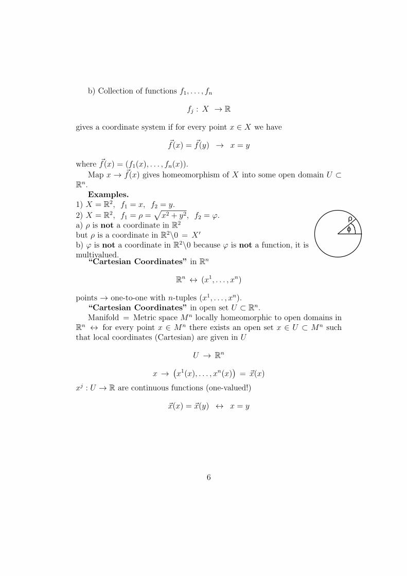
2) X = R2, f1 = ρ =√x2 + y2, f2 = φ.
a) ρ is not a coordinate in R2
but ρ is a coordinate in R2\0 = X ′
b) φ is not a coordinate in R2\0 because φ is not a function, it ismultivalued.
ρϕ
“Cartesian Coordinates” in Rn
Rn ↔ (x1, . . . , xn)
points → one-to-one with n-tuples (x1, . . . , xn).“Cartesian Coordinates” in open set U ⊂ Rn.Manifold = Metric space Mn locally homeomorphic to open domains in
Rn ↔ for every point x ∈ Mn there exists an open set x ∈ U ⊂ Mn suchthat local coordinates (Cartesian) are given in U
U → Rn
x →(x1(x), . . . , xn(x)
)= x(x)
xj : U → R are continuous functions (one-valued!)
x(x) = x(y) ↔ x = y
6
Lecture 2. Manifolds and Atlases.
Manifolds: = Hausdorff (or metric) spaces such that they are “locallyeuclidean”: for every x ∈ M there exists an open set x ∈ U with homeo-morphism
φU : U → Rn = (x1, . . . , xn) (so U ⊂ Rn)
The set U represents a “Chart” in the “Atlas” onM . “Local coordinates”in U (near x)
x → Rn −→xi
R
are continuous functions in U and
x(x) = x(y) ↔ x = y
for any two points x, y in U .For a given “Atlas” Uα, covering M , we can introduce “Transition
Maps” in the intersections U ∩ V , where U = Uα, V = Uβ. Thus, forany x ∈ U ∩ V we can use the local coordinates (x1, . . . , xn) (xα in U)or (y1, . . . , yn) (xβ in V ). The functions xi(y1, . . . , yn) and yk(x1, . . . , xn)represent maps of euclidean domains
xi(y), i = 1, . . . , n, yk(x), k = 1, . . . , n
Definition. Manifold M is C∞ if all the functions xi(y) (given by Atlas forevery pair U , V ) are C∞.Statement. In the C∞ Atlas all Jacobians det |∂xi/∂yk| are non-zero.
Proof. Since x(y) and y(x) are both C∞ we have det |∂xi/∂yk| = 0.∑k
∂xi
∂yk∂yk
∂xj= δij
Summation agreement: we do not write∑
, so, in our notations
∂xi
∂yk∂yk
∂xj= δij
Definition: Oriented Atlas is such that all det |∂xi/∂yk| > 0Oriented manifold: = there exists an oriented Atlas.Examples:
7
S2−x
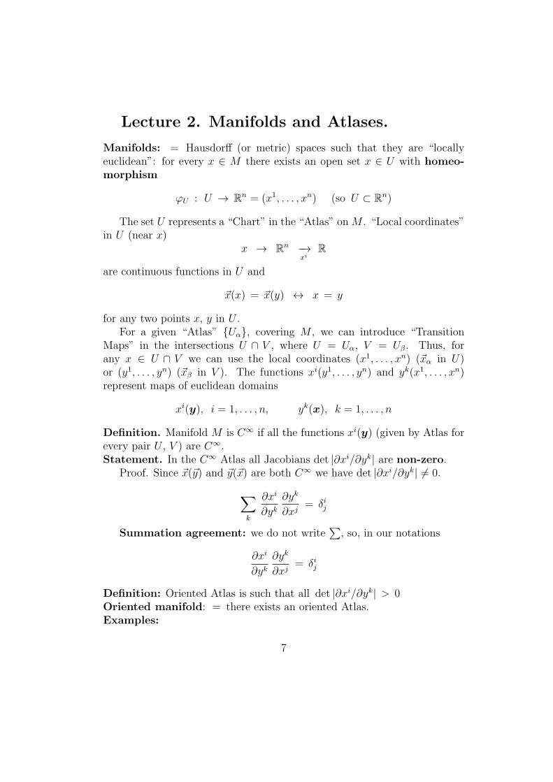
xn = 2:S2 is oriented manifold.RP2 is NOT.(x,−x) is one point in RP2.
Definitions.1) C∞ - function in C∞ - manifold M with given Atlas of Charts:
M → R is C∞ in every Chart.2) C∞ - map
MF−→ N
(Uα) (Vβ)
is C∞ in every Chart. In other words, for every pair Uα, Vβ the correspondingfunctions ykβ(x
1α, . . . , x
nα) are C
∞ in F−1(Vβ) ∩ Uα.Rank of the map F :M → N at the point x ∈M :
rkxF = rk
(∂ykβ∂xiα
)∣∣∣∣∣x
where UαF−→ Vβ
(x) (y)
Statement. Rank of the map at the point x does not depend on the choiceof Atlas.
Proof. Let Uα, Vβ be Euclidean domains giving the charts of the manifoldsM and N and the functions y(x) be represented by the map
UαF−→ Vβ
(x) (y)
Consider two other domains Wα and Xβ with coordinates x and y repre-senting two other charts containing the points x and F (x) respectively. Letus consider the functions y(x) = y(y(x(x))) defined by the map
Wα → UαF−→ Vβ → Xβ
(x) (x) (y) (y)
We have∂yi
∂xj=
∂yi
∂yk∂yk
∂xs∂xs
∂xj,
where rk |∂yi/∂yk| = 0, rk |∂xs/∂xj| = 0.
8
Conclusion
rk
∣∣∣∣ ∂yi∂xj
∣∣∣∣ = rk
∣∣∣∣ ∂yi∂xj
∣∣∣∣Statement is proved.
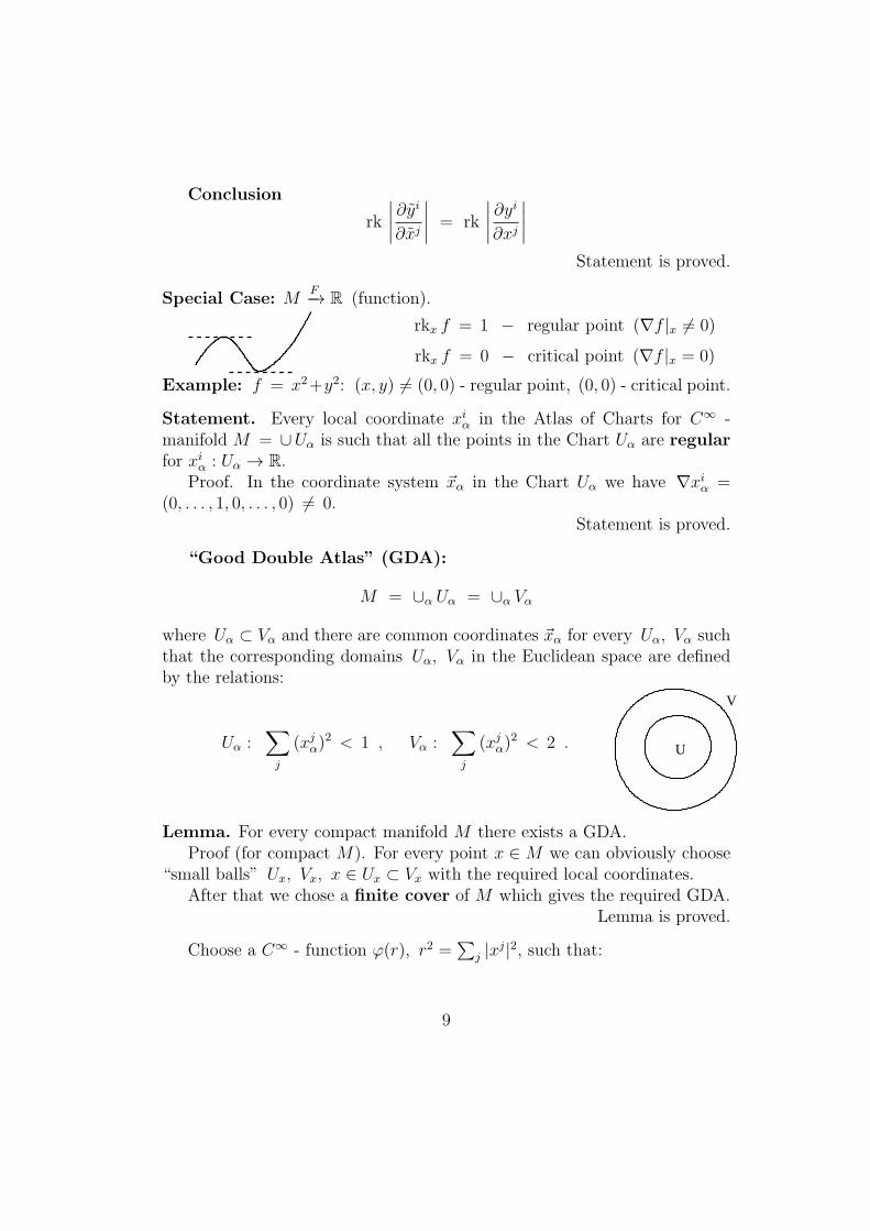
Special Case: MF−→ R (function).
rkx f = 1 − regular point (∇f |x = 0)
rkx f = 0 − critical point (∇f |x = 0)
Example: f = x2+y2: (x, y) = (0, 0) - regular point, (0, 0) - critical point.
Statement. Every local coordinate xiα in the Atlas of Charts for C∞ -manifold M = ∪Uα is such that all the points in the Chart Uα are regularfor xiα : Uα → R.
Proof. In the coordinate system xα in the Chart Uα we have ∇xiα =(0, . . . , 1, 0, . . . , 0) = 0.
Statement is proved.
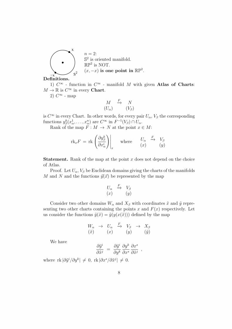
“Good Double Atlas” (GDA):
M = ∪α Uα = ∪α Vα
where Uα ⊂ Vα and there are common coordinates xα for every Uα, Vα suchthat the corresponding domains Uα, Vα in the Euclidean space are definedby the relations:
Uα :∑j
(xjα)2 < 1 , Vα :
∑j
(xjα)2 < 2 . U
V
Lemma. For every compact manifold M there exists a GDA.Proof (for compact M). For every point x ∈M we can obviously choose
“small balls” Ux, Vx, x ∈ Ux ⊂ Vx with the required local coordinates.After that we chose a finite cover of M which gives the required GDA.
Lemma is proved.
Choose a C∞ - function φ(r), r2 =∑
j |xj|2, such that:
9
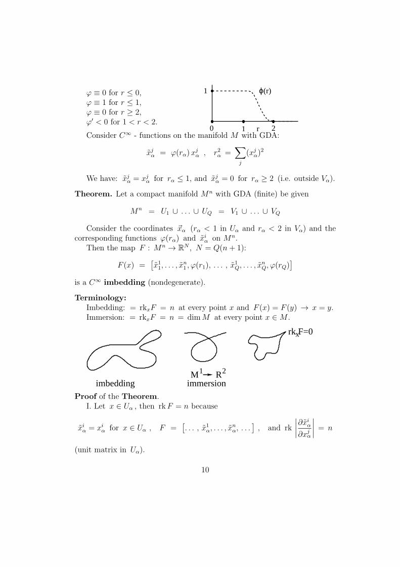
φ ≡ 0 for r ≤ 0,φ ≡ 1 for r ≤ 1,φ ≡ 0 for r ≥ 2,φ′ < 0 for 1 < r < 2.
1
10 2r
ϕ(r)
Consider C∞ - functions on the manifold M with GDA:
xjα = φ(rα)xjα , r2α =
∑j
(xjα)2
We have: xjα = xjα for rα ≤ 1, and xjα = 0 for rα ≥ 2 (i.e. outside Vα).
Theorem. Let a compact manifold Mn with GDA (finite) be given
Mn = U1 ∪ . . . ∪ UQ = V1 ∪ . . . ∪ VQ
Consider the coordinates xα (rα < 1 in Uα and rα < 2 in Vα) and thecorresponding functions φ(rα) and xiα on Mn.
Then the map F : Mn → RN , N = Q(n+ 1):
F (x) =[x11, . . . , x
n1 , φ(r1), . . . , x
1Q, . . . , x
nQ, φ(rQ)
]is a C∞ imbedding (nondegenerate).
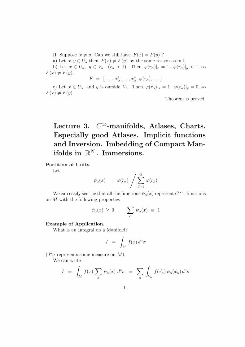
Terminology:Imbedding: = rkxF = n at every point x and F (x) = F (y) → x = y.Immersion: = rkxF = n = dimM at every point x ∈M .
M 1 R2
imbedding immersion
rk F=0x
Proof of the Theorem.I. Let x ∈ Uα , then rkF = n because
xiα = xiα for x ∈ Uα , F =[. . . , x1α, . . . , x
nα, . . .
], and rk
∣∣∣∣∂xiα∂xjα
∣∣∣∣ = n
(unit matrix in Uα).
10
II. Suppose x = y. Can we still have F (x) = F (y) ?a) Let x, y ∈ Uα then F (x) = F (y) by the same reason as in I.b) Let x ∈ Uα, y ∈ Vα (rα > 1). Then φ(rα)|x = 1, φ(rα)|y < 1, so
F (x) = F (y),F =
[. . . , x1α, . . . , x
nα, φ(rα), . . .
]c) Let x ∈ Uα, and y is outside Vα. Then φ(rα)|x = 1, φ(rα)|y = 0, so
F (x) = F (y).Theorem is proved.
Lecture 3. C∞-manifolds, Atlases, Charts.
Especially good Atlases. Implicit functions
and Inversion. Imbedding of Compact Man-
ifolds in RN . Immersions.
Partition of Unity.Let
ψα(x) = φ(rα)
/Q∑β=1
φ(rβ)
We can easily see the that all the functions ψα(x) represent C∞ - functions
on M with the following properties
ψα(x) ≥ 0 ,∑α
ψα(x) ≡ 1
Example of Application.What is an Integral on a Manifold?
I =
∫M
f(x) dnσ
(dnσ represents some measure on M).We can write
I =
∫M
f(x)∑α
ψα(x) dnσ =
∑α
∫Vα
f(xα)ψα(xα) dnσ
11
We can see now that I is represented as a sum of ordinary integralsover local domains where we can also put in local coordinates: dnσ =gα(xα) dx
1α . . . dx
nα.
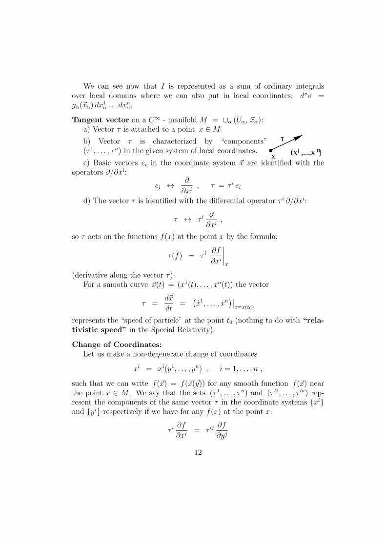
Tangent vector on a C∞ - manifold M = ∪α (Uα, xα):a) Vector τ is attached to a point x ∈M .
b) Vector τ is characterized by “components”(τ 1, . . . , τn) in the given system of local coordinates.
τ
x (x ,...,x )1 n
c) Basic vectors ei in the coordinate system x are identified with theoperators ∂/∂xi:
ei ↔∂
∂xi, τ = τ i ei
d) The vector τ is identified with the differential operator τ i ∂/∂xi:
τ ↔ τ i∂
∂xi,
so τ acts on the functions f(x) at the point x by the formula:
τ(f) = τ i∂f
∂xi
∣∣∣∣x
(derivative along the vector τ).For a smooth curve x(t) = (x1(t), . . . , xn(t)) the vector
τ =dx
dt=
(x1, . . . , xn
)∣∣x=x(t0)
represents the “speed of particle” at the point t0 (nothing to do with “rela-tivistic speed” in the Special Relativity).
Change of Coordinates:Let us make a non-degenerate change of coordinates
xi = xi(y1, . . . , yn) , i = 1, . . . , n ,
such that we can write f(x) = f(x(y)) for any smooth function f(x) nearthe point x ∈ M . We say that the sets (τ 1, . . . , τn) and (τ ′1, . . . , τ ′n) rep-resent the components of the same vector τ in the coordinate systems xiand yi respectively if we have for any f(x) at the point x:
τ i∂f
∂xi= τ ′j
∂f
∂yj
12
By definition, we can write
τ i∂f
∂xi= τ ′j
∂xi
∂yj∂f
∂xi,
so we come to the conclusion
τ i = τ ′j∂xi
∂yj
(summation over j is assumed).In the same way, for the inverse transformation y = y(x) we can write
τ ′j = τ i∂yj
∂xi
where∂xi
∂yj∂yj
∂xk= δik
Every C∞ - map is given locally by its linear part and the smaller terms
yi = F i(x1, . . . , xn) = Const +n∑j=1
Aij xj + O(||x||2)
(near x = 0).
Inversion of Map (C∞).Let us have a map
F : Rn → Rn , x0 → y0(x) (y)
given in coordinate form by the functions yi = yi(x1, . . . , xn).If we have the relation
det
∣∣∣∣ ∂yi∂xk
∣∣∣∣ ∣∣∣∣x0
= 0
then there exist open sets V ∋ x0, U ∋ y0 and a map
G : Rn → Rn , y0 → x0 ,(y) (x)
13
defined in the set U , such that for x ∈ V , y ∈ U we have the relations
G (F (x)) ≡ x , F (G(y)) ≡ y
Naturally, we have in this case
∂xi
∂yj
∣∣∣∣y0
∂yj
∂xk
∣∣∣∣x0
= δik , i.e.
(∂x
∂y
)∣∣∣∣y0
(∂y
∂x
)∣∣∣∣x0
= I
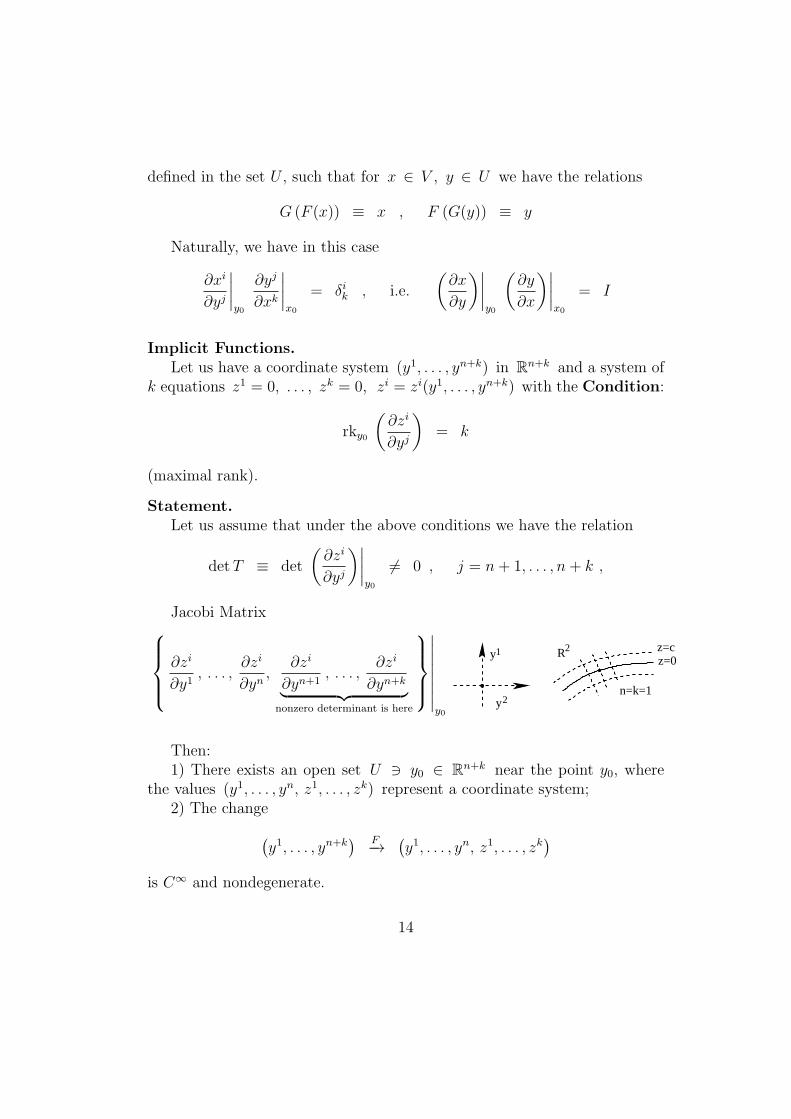
Implicit Functions.Let us have a coordinate system (y1, . . . , yn+k) in Rn+k and a system of
k equations z1 = 0, . . . , zk = 0, zi = zi(y1, . . . , yn+k) with the Condition:
rky0
(∂zi
∂yj
)= k
(maximal rank).
Statement.Let us assume that under the above conditions we have the relation
detT ≡ det
(∂zi
∂yj
)∣∣∣∣y0
= 0 , j = n+ 1, . . . , n+ k ,
Jacobi Matrix∂zi
∂y1, . . . ,
∂zi
∂yn,
∂zi
∂yn+1, . . . ,
∂zi
∂yn+k︸ ︷︷ ︸nonzero determinant is here
∣∣∣∣∣∣∣∣y0
R2y1
y2
z=0z=c
n=k=1
Then:1) There exists an open set U ∋ y0 ∈ Rn+k near the point y0, where
the values (y1, . . . , yn, z1, . . . , zk) represent a coordinate system;2) The change(
y1, . . . , yn+k) F−→
(y1, . . . , yn, z1, . . . , zk
)is C∞ and nondegenerate.
14
Proof.Easy to see that the Jacobian Matrix of the transformation F can be
written in the form:
J =
1 0 . . . 0 ∂z1/∂y1 . . . ∂zk/∂y1
0 1 . . . 0 ∂z1/∂y2 . . . ∂zk/∂y2
......
. . ....
.... . .
...0 0 . . . 1 ∂z1/∂yn . . . ∂zk/∂yn
0 0 . . . 0 ∂z1/∂yn+1 . . . ∂zk/∂yn+1
......
. . ....
.... . .
...0 0 . . . 0 ∂z1/∂yn+k . . . ∂zk/∂yn+k
We immediately get then det Jy0 = detT = 0. So, we get our statement
from the Inversion Theorem.Statement is proved.
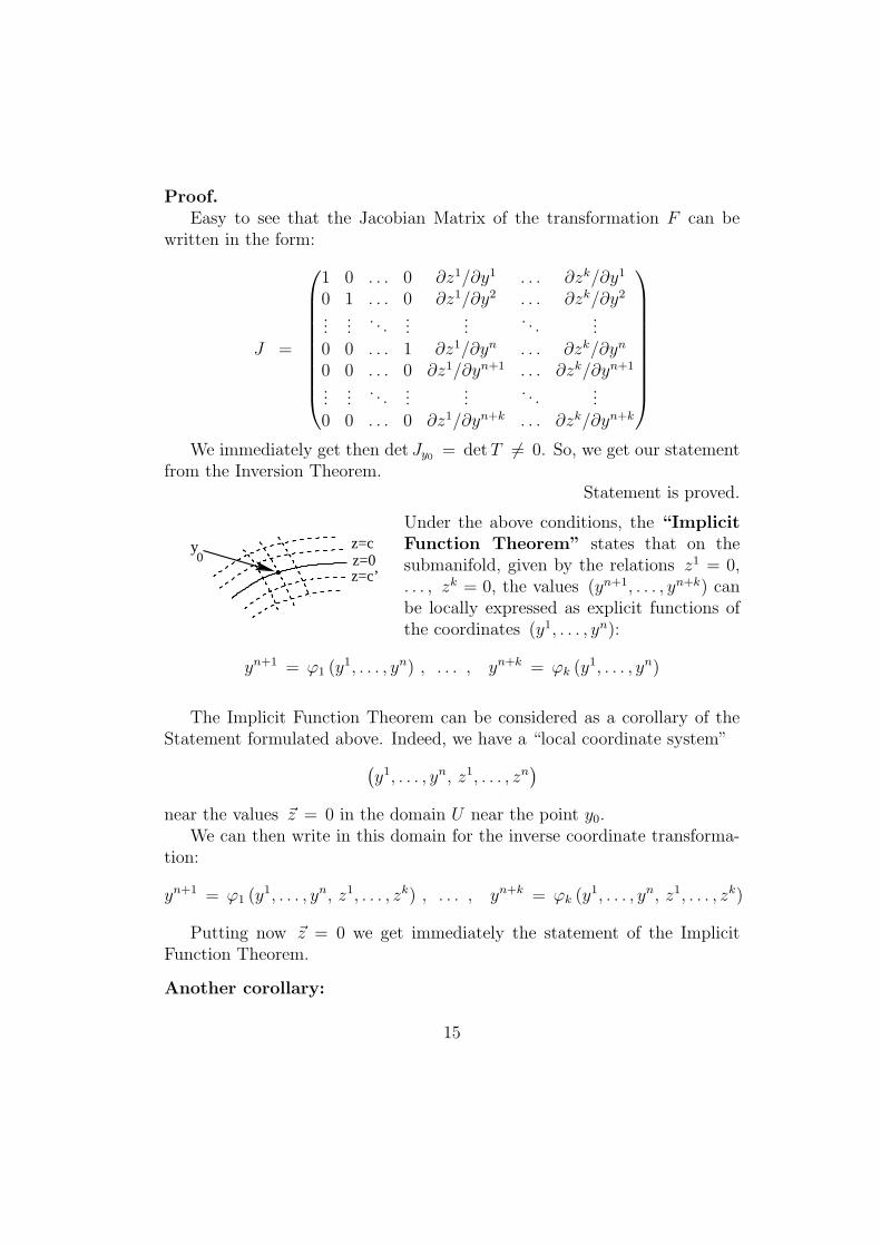
y0 z=0
z=c
z=c’
Under the above conditions, the “ImplicitFunction Theorem” states that on thesubmanifold, given by the relations z1 = 0,. . . , zk = 0, the values (yn+1, . . . , yn+k) canbe locally expressed as explicit functions ofthe coordinates (y1, . . . , yn):
yn+1 = φ1 (y1, . . . , yn) , . . . , yn+k = φk (y
1, . . . , yn)
The Implicit Function Theorem can be considered as a corollary of theStatement formulated above. Indeed, we have a “local coordinate system”(
y1, . . . , yn, z1, . . . , zn)
near the values z = 0 in the domain U near the point y0.We can then write in this domain for the inverse coordinate transforma-
tion:
yn+1 = φ1 (y1, . . . , yn, z1, . . . , zk) , . . . , yn+k = φk (y
1, . . . , yn, z1, . . . , zk)
Putting now z = 0 we get immediately the statement of the ImplicitFunction Theorem.
Another corollary:
15
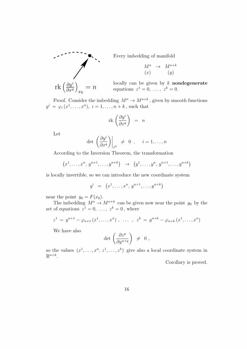
rk
(
∂yi
∂xq
)
x0
= n
Every imbedding of manifold
Mn → Mn+k
(x) (y)
locally can be given by k nondegenerateequations z1 = 0, . . . , zk = 0.
Proof. Consider the imbedding Mn →Mn+k , given by smooth functionsyi = φi (x
1, . . . , xn), i = 1, . . . , n+ k , such that
rk
(∂yi
∂xq
)= n
Let
det
(∂yi
∂xq
)∣∣∣∣x0= 0 , i = 1, . . . , n
According to the Inversion Theorem, the transformation(x1, . . . , xn, yn+1, . . . , yn+k
)→
(y1, . . . , yn, yn+1, . . . , yn+k
)is locally invertible, so we can introduce the new coordinate system
y′ =(x1, . . . , xn, yn+1, . . . , yn+k
)near the point y0 = F (x0).
The imbedding Mn →Mn+k can be given now near the point y0 by theset of equations z1 = 0, . . . , zk = 0 , where
z1 = yn+1 − φn+1 (x1, . . . , xn) , . . . , zk = yn+k − φn+k (x1, . . . , xn)
We have also
det
(∂zp
∂yn+q
)= 0 ,
so the values (x1, . . . , xn, z1, . . . , zk) give also a local coordinate system inRn+k.
Corollary is proved.
16
Lecture 4. Manifolds and Submanifolds: Im-
plicit functions and Inversion. Vectors and
Covectors.
According to the previous lecture, we can formulate here the following
Statement.Let us have an imbedding
F : Mn → Nn+k , (rkxF = n , ∀x , F (x) = F (y) , ∀x = y) ,
such that either Mn is compact or for every compact set X ⊂ N theintersection X ∩ F (M) is compact.
Then:For every point x ∈ Mn ⊂ Nn+k there exists local coordinate system
(x1, . . . , xn, z1, . . . , zk) in some U ∋ x such that the submanifold Mn isgiven in U by the system
z1 = 0 , . . . , zk = 0
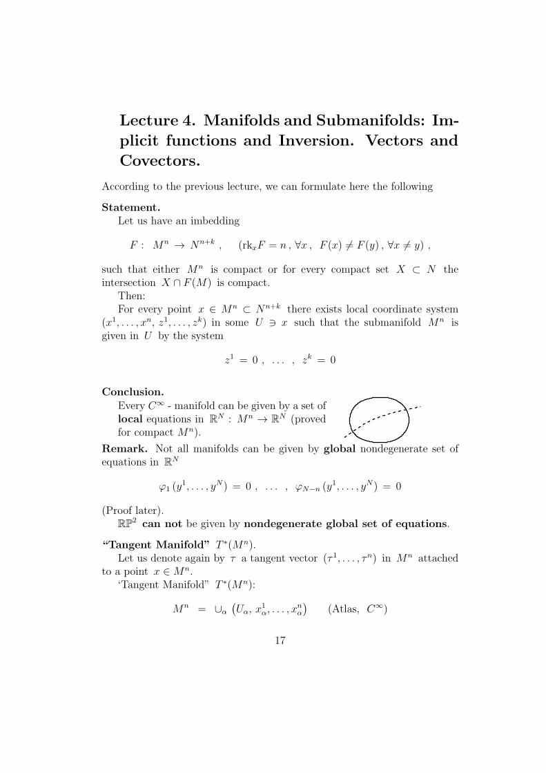
Conclusion.Every C∞ - manifold can be given by a set oflocal equations in RN : Mn → RN (provedfor compact Mn).
Remark. Not all manifolds can be given by global nondegenerate set ofequations in RN
φ1 (y1, . . . , yN) = 0 , . . . , φN−n (y
1, . . . , yN) = 0
(Proof later).RP2 can not be given by nondegenerate global set of equations.
“Tangent Manifold” T ∗(Mn).Let us denote again by τ a tangent vector (τ 1, . . . , τn) in Mn attached
to a point x ∈Mn.‘Tangent Manifold” T ∗(Mn):
Mn = ∪α(Uα, x
1α, . . . , x
nα
)(Atlas, C∞)
17
T ∗(Mn) = ∪α(Uα × Rn , x1α, . . . , x
nα , τ
1, . . . , τn)
Change of coordinates:Let us put in the intersection of Charts Uα and Uβ : x = xα, y = xβ.
We have then
xi = xi(y) = xi(y1, . . . , yn) (in Uα ∩ Uβ)
The components of the same vector in the coordinates (x) and (y):
(x, τ) ↔ (y, τ ′)
are connected by the relations:
τ i = τ ′j∂xi
∂yj
(∑j
is assumed
)
Covectors (η1, . . . , ηn) are attached to the points x ∈Mn.Change of coordinates
(x, η) ↔ (y, η′)
η′j = ηi∂xi
∂yj, ηi = η′j
∂yj
∂xi
T∗(Mn) = ∪α
(Uα × Rn , x1α, . . . , x
nα , η1, . . . , ηn
)Scalar product (invariant):
⟨τ , η⟩ = τ i ηi
Conclusion: Spaces of vectors and covectors are dual.Basis:
vectors : ei ↔∂
∂xi
covectors : ei ↔ d xi
Vector field : f i∂
∂xi(Vector fields)
Covector field : gi dxi (Differential 1− forms)
18
Vector Fields = Dynamical Systems (Autonomous)
Integration of 1-forms along the path: let
ω = gi(x) dxi
and the path is given by a piecewisesmooth one-parametric curve
x(t) =(x1(t), . . . , xn(t)
) B
A
x(t)
Definition.∫x(t)
ω =
∫ B
A
gi(x) dxi =
∫ t1
t0
(gi (x(t))
dxi
dt
)dt
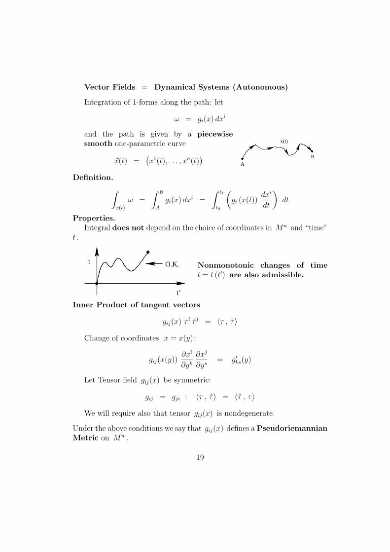
Properties.Integral does not depend on the choice of coordinates in Mn and “time”
t .
t
t’
O.K. Nonmonotonic changes of timet = t (t′) are also admissible.
Inner Product of tangent vectors
gij(x) τi τ j = ⟨τ , τ⟩
Change of coordinates x = x(y):
gij(x(y))∂xi
∂yk∂xj
∂ys= g′ks(y)
Let Tensor field gij(x) be symmetric:
gij = gji : ⟨τ , τ⟩ = ⟨τ , τ⟩
We will require also that tensor gij(x) is nondegenerate.
Under the above conditions we say that gij(x) defines aPseudoriemannianMetric on Mn .
19
Types of inner products (“Types of Geometry”):gij dx
i dxj > 0 - Riemannian Metric.Special Types (p, q) of Pseudoriemannian metric:
p = 0 : - Riemannianp = 1 : - Lorentzianp = q : - Ultrahyperbolic
Theorem.In every C∞ - manifold there exists a C∞ Riemannian Metric.
Proof. Take GDA (Good Double Atlas)
Mn = U1 ∪ . . . ∪ UQ = V1 ∪ . . . ∪ VQ
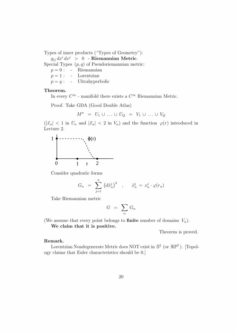
(|xα| < 1 in Uα and |xα| < 2 in Vα) and the function φ(r) introduced inLecture 2.
1
10 2r
ϕ(r)
Consider quadratic forms
Gα =n∑j=1
(dxjα)2
, xjα = xjα · φ(rα)
Take Riemannian metric
G =∑α
Gα
(We assume that every point belongs to finite number of domains Vα).We claim that it is positive.
Theorem is proved.
Remark.Lorentzian Nondegenerate Metric does NOT exist in S2 (or RP2 ). [Topol-
ogy claims that Euler characteristics should be 0.]
20
Homework 1.
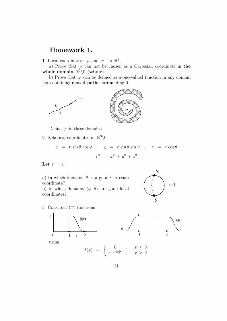
1. Local coordinates: ρ and φ in R2 .a) Prove that ρ can not be chosen as a Cartesian coordinate in the
whole domain R2\0 (whole).b) Prove that φ can be defined as a one-valued function in any domain
not containing closed paths surrounding 0 .
U
U
0
Define φ in these domains.
2. Spherical coordinates in R3\0
x = r sin θ cosφ , y = r sin θ sinφ , z = r cos θ
r2 = x2 + y2 + z2
Let r = 1 .
a) In which domains θ is a good Cartesiancoordinate?b) In which domains (φ, θ) are good localcoordinates?
N
S
r=1
3. Construct C∞ functions
ϕ(r)1
10 2r
ψ(r)
1
0
1
−1
using
f(x) =
0 , x ≤ 0
e−1/|x|2 , x ≥ 0
21
Lecture 5. Manifolds and vectors fields. Im-
portant Examples.
Classes of manifolds:a) All C∞ - manifolds Mn ⊂ RN for given N .b) Manifolds defined by the Global Nondegenerate systems of Equations
in RN
f1 = 0 , . . . , fN−n = 0
(Important cases: n = 2, N = n+ 1 = 3).
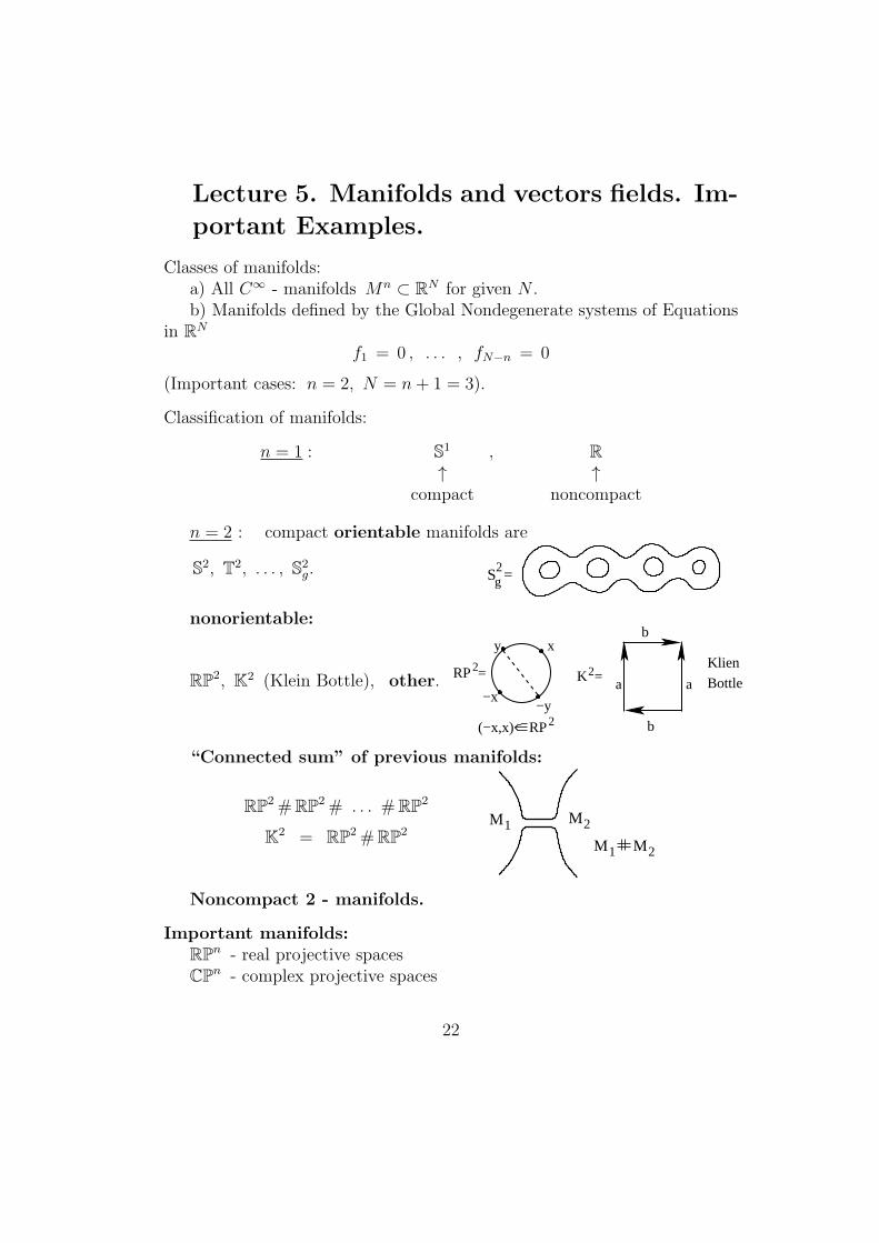
Classification of manifolds:
n = 1 : S1 , R↑ ↑
compact noncompact
n = 2 : compact orientable manifolds are
S2, T2, . . . , S2g. S =g
2
nonorientable:
RP2, K2 (Klein Bottle), other. RP =2
RP2
K =2
y
−y−x
x
(−x,x)
b
b
Bottle
Klien
a a
“Connected sum” of previous manifolds:
RP2 #RP2 # . . . #RP2
K2 = RP2#RP2M2M1
M1 M2
Noncompact 2 - manifolds.
Important manifolds:RPn - real projective spacesCPn - complex projective spaces
22
QPn - “quaternionic” projective spacesGroups: GLn(R), GLn(C), SLn(R), SLn(C), On ⊃ SOn, Op,q ⊃
SOp,q (case p = 1 - Lorentz Groups), Un ⊃ SUn, Up,q ⊃ SUp,qStiefel ManifoldsGrassmann ManifoldsIsometry groups of Rn
Isometry groups of Rp,q
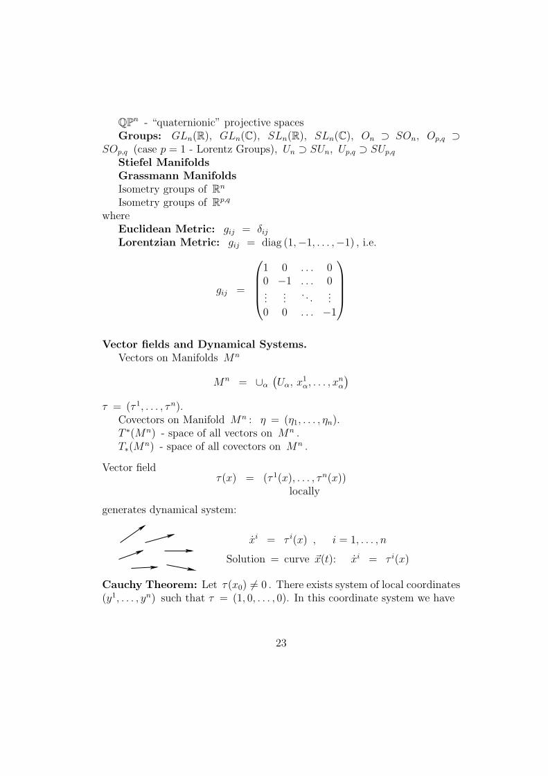
whereEuclidean Metric: gij = δijLorentzian Metric: gij = diag (1,−1, . . . ,−1) , i.e.
gij =
1 0 . . . 00 −1 . . . 0...
.... . .
...0 0 . . . −1
Vector fields and Dynamical Systems.
Vectors on Manifolds Mn
Mn = ∪α(Uα, x
1α, . . . , x
nα
)τ = (τ 1, . . . , τn).
Covectors on Manifold Mn : η = (η1, . . . , ηn).T ∗(Mn) - space of all vectors on Mn .T∗(M
n) - space of all covectors on Mn .
Vector fieldτ(x) = (τ 1(x), . . . , τn(x))
locally
generates dynamical system:
xi = τ i(x) , i = 1, . . . , n
Solution = curve x(t): xi = τ i(x)
Cauchy Theorem: Let τ(x0) = 0 . There exists system of local coordinates(y1, . . . , yn) such that τ = (1, 0, . . . , 0). In this coordinate system we have
23
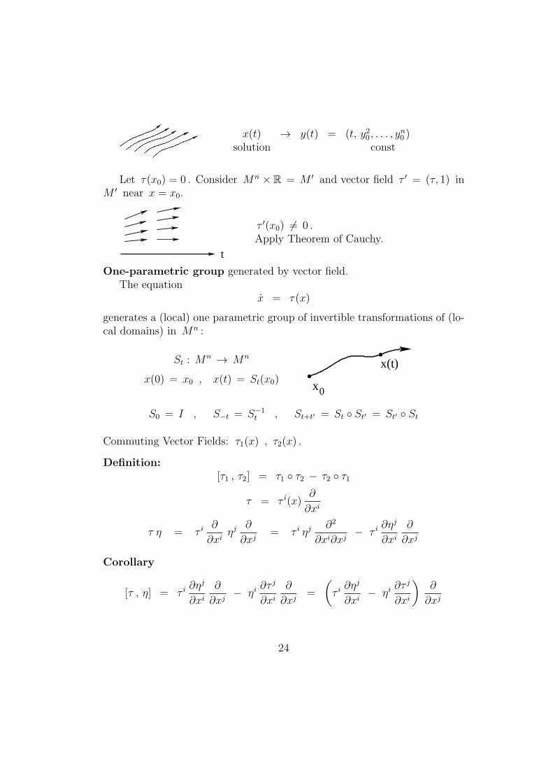
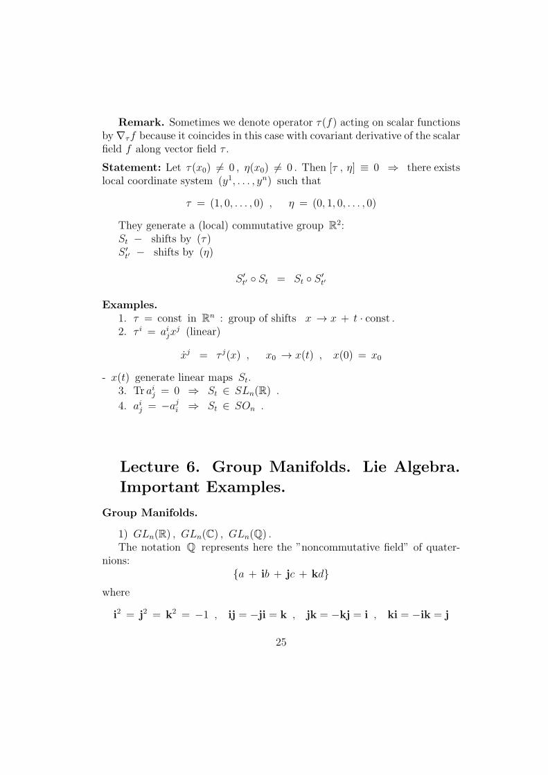
x(t) → y(t) = (t, y20, . . . , yn0 )
solution const
Let τ(x0) = 0 . Consider Mn × R = M ′ and vector field τ ′ = (τ, 1) inM ′ near x = x0.
t
τ ′(x0) = 0 .Apply Theorem of Cauchy.
One-parametric group generated by vector field.The equation
x = τ(x)
generates a (local) one parametric group of invertible transformations of (lo-cal domains) in Mn :
St : Mn → Mn
x(0) = x0 , x(t) = St(x0) x0
x(t)
S0 = I , S−t = S−1t , St+t′ = St St′ = St′ St
Commuting Vector Fields: τ1(x) , τ2(x) .
Definition:[τ1 , τ2] = τ1 τ2 − τ2 τ1
τ = τ i(x)∂
∂xi
τ η = τ i∂
∂xiηj
∂
∂xj= τ i ηj
∂2
∂xi∂xj− τ i
∂ηj
∂xi∂
∂xj
Corollary
[τ , η] = τ i∂ηj
∂xi∂
∂xj− ηi
∂τ j
∂xi∂
∂xj=
(τ i∂ηj
∂xi− ηi
∂τ j
∂xi
)∂
∂xj
24
Remark. Sometimes we denote operator τ(f) acting on scalar functionsby∇τf because it coincides in this case with covariant derivative of the scalarfield f along vector field τ .
Statement: Let τ(x0) = 0 , η(x0) = 0 . Then [τ , η] ≡ 0 ⇒ there existslocal coordinate system (y1, . . . , yn) such that
τ = (1, 0, . . . , 0) , η = (0, 1, 0, . . . , 0)
They generate a (local) commutative group R2:St − shifts by (τ)S ′t′ − shifts by (η)
S ′t′ St = St S ′
t′
Examples.1. τ = const in Rn : group of shifts x → x + t · const .2. τ i = aijx
j (linear)
xj = τ j(x) , x0 → x(t) , x(0) = x0
- x(t) generate linear maps St.3. Tr aij = 0 ⇒ St ∈ SLn(R) .
4. aij = −aji ⇒ St ∈ SOn .
Lecture 6. Group Manifolds. Lie Algebra.
Important Examples.
Group Manifolds.
1) GLn(R) , GLn(C) , GLn(Q) .The notation Q represents here the ”noncommutative field” of quater-
nions:a + ib + jc + kd
where
i2 = j2 = k2 = −1 , ij = −ji = k , jk = −kj = i , ki = −ik = j
25
dimGLn(R) = n2
dimGLn(C) = 2n2
dimGLn(Q) = 4n2
Question: prove that GLn(R) has 2 components. GLn(C) is connected.
2) SLn(R) , SLn(C) : det = 1Equation : detA = 1 in Rn2
or in Cn2
Is this equation nondegenerate ?
3) On , AAt = I ,
a) Is this set of equations NONDEGENERATE in GLn(R) ∈ Rn2?
b) Is SOn - connected manifold?c) dimOn = n(n− 1)/2
4) Op,q : ⟨Aη , Aζ⟩ = ⟨η , ζ⟩a) p = 1 , q = n , ⟨η , ζ⟩ = η0ζ0 −
∑nα=1 η
αζα , (1, n)
b) ⟨η , ζ⟩ =∑p
α=1 ηαζα −
∑p+qα=p+1 η
αζα , (p, q)
5) Unitary group: ζ, η ∈ Cn
⟨ζ , η⟩ = ⟨η , ζ⟩ =∑i≤p
ζ i ηi −∑i>p
ζ i ηi
Up,q : ⟨Aζ , Aη⟩ = ⟨ζ , η⟩ , (q = 0 : Un)
SUn , SUp,q : detA = 1
How to introduce local coordinates in the group manifold Mn = G ?Let A(t) ∈ G , A(0) = I .
dA
dt
∣∣∣∣t=0
= B ∈ Lie Algebra
Another form
Lie Algebra → dA
dtA−1 or A−1 dA
dt
Groups SOn , On :
⟨A(t)ζ , A(t)η⟩ = ⟨ζ , η⟩ ,d
dt⟨A(t)ζ , A(t)η⟩ = 0 ,
26
A(t) = A(0) + A(0) t + O(t2) , A(0) = 1↑B
Lemma 1: Bt = −B (i.e. At(0) = −A(0) ).
Proof.
⟨A(t)ζ , A(t)η⟩ = ⟨ζ , η⟩ + t [⟨Bζ , η⟩ + ⟨ζ , Bη⟩] + O(t2)
d
dt⟨A(t)ζ , A(t)η⟩
∣∣∣∣t=0
= 0 ⇒ ⟨Bζ , η⟩ + ⟨ζ , Bη⟩ = 0
i.e.⟨Bζ , η⟩ ≡ − ⟨ζ , Bη⟩
Lemma is proved.
Lemma 2: ∃ ϵ > 0 such that for any A ∈ SOn , ||A − I|| < ϵ we haveA = eB , Bt = −B .
Proof.For small enough ϵ consider the convergent series
B = log (I + A− I) = A− I − (A− I)2/2 + (A− I)3/3 − . . .
Bt = log (I + At − I) = At − I − (At − I)2/2 + (At − I)3/3 − . . .
We can write then: A = eB , At = eBt. Besides that, from the
commutativity of all the terms of the series we can write also:
eB+Bt
= AAt = I
which implies Bt = −B for small enough B .Lemma is proved.
Local coordinates in GLn(R) near I can be also taken from a small ballin the space Rn2
= space of matrices.
Lemma 3: For small enough B we have: TrB = 0 ⇔ det eB = 1.
Proof.For the diagonal matrices B = diag (b1, . . . , bn) we obviously have the
relation det eB =∏ebi = exp (TrB) . The same property is then also
27
evident for the diagonalizable matrices B = S−1 diag (b1, . . . , bn) Sfrom the series representation of the matrix eB . Since the set of diagonaliz-able matrices is dense in the matrix space and the functions exp (TrB) anddet eB are analytic functions of the matrix entries we actually have
det eB = eTrB
for any matrix B . The statement of the Lemma for small enough B followsthen from the properties of the function ex .
Lemma is proved.
We can see then that in the local coordinate system in GLn(R) , givenby the entries of the matrix B near I ∈ GLn(R) , the equation detA = 1has the form TrB = 0 .Conclusion. This equation is linear and NONDEGENERATE.
Group SOn : Equations for SOn in the coordinate system, given by theentries of B near I ∈ GLn(R) , have the form Bt = −B .
Unitary group A At = I.Un ⊂ GLn(C) , we can put again A = eB near I = GLn(C) and
introduce a local coordinate system, given by the entries of B in Cn2=
R2n2. In this coordinate system:
a) Group SLn(C) is given by equation TrB = 0 (2 real equations).b) Group Un is given by equations Bt = −B (Bt = −B) , i.e. n2
linear equations over R .dimUn = n2 (over R ). U1 = S1 = SO2 dimU2 = 4 , is SU2 = S3 ?
A ∈ SU2 : ⇒ A =
(a bc d
),
where ac+ bd = 0 , |a|2 + |b|2 = 1 , |c|2 + |d|2 = 1 , |ad− bc| = 1 .So, we have
A =
(a b−b a
), |a|2 + |b|2 = 1 ,
i.e. SU2 = S3 .
Quaternion Group: GLn(Q) .
Q : q = a + ib + jc + kd
28
i2 = j2 = k2 = −1 , ij = −ji = k , jk = −kj = i , ki = −ik = j
q ≡ a − ib − jc − kd
GL2(Q) = q : q q = 1 = a2 + b2 + c2 + d2 = 1 = S3 = SU2
Pauli matrices:
i σx =
(0 1−1 0
), i σy =
(0 ii 0
), i σz =
(i 00 −i
)Correspondence to the basic quaternions (i, j, k):
i σx ↔ i , i σy ↔ j , i σz ↔ k
SO3 = SU2/Z2 = S3/Z2 = RP3
Indeed, consider the norm-conserving transformations
q → q1 q q1 , q1 q1 = 1
Space Span 1 and the orthogonal space Span i, j, k are invariant.Two transformations coincide iff : q′1 = ±q1 .
SO4 = S3 × S3/Z2
Consider the transformations
q → q1 q q2 , q1 q1 = 1 , q2 q2 = 1
Two transformations coincide iff : (q′1 , q′2) = ±(q1 , q2) .
Lecture 7. Group Manifolds: Compact Lie
groups. Most important Examples. Non-
compact Lie groups. Most important Exam-
ples. Lie Algebras. Gradient-like Systems.
Group manifolds.
29
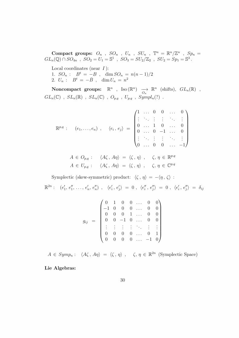
Compact groups: On , SOn , Un , SUn , Tn = Rn/Zn , Spn =GLn(Q) ∩ SO4n , SO2 = U1 = S1 , SO3 = SU2/Z2 , SU2 = Sp1 = S3 .
Local coordinates (near I ):1. SOn : Bt = −B , dimSOn = n(n− 1)/22. Un : Bt = −B , dimUn = n2
Noncompact groups: Rn , Iso (Rn) −→On
Rn (shifts), GLn(R) ,
GLn(C) , SLn(R) , SLn(C) , Op,q , Up,q , Sympln(?) .
Rp,q : (e1, . . . , en) , ⟨ei , ej⟩ =
1 . . . 0 0 . . . 0...
. . ....
.... . .
...0 . . . 1 0 . . . 00 . . . 0 −1 . . . 0...
. . ....
.... . .
...0 . . . 0 0 . . . −1
A ∈ Op,q : ⟨Aζ , Aη⟩ = ⟨ζ , η⟩ , ζ, η ∈ Rp,q
A ∈ Up,q : ⟨Aζ , Aη⟩ = ⟨ζ , η⟩ , ζ, η ∈ Cp,q
Symplectic (skew-symmetric) product: ⟨ζ , η⟩ = −⟨η , ζ⟩ :
R2n : (e′1, e′′1, . . . , e
′n, e
′′n) , ⟨e′i , e′j⟩ = 0 , ⟨e′′i , e′′j ⟩ = 0 , ⟨e′i , e′′j ⟩ = δij
gij =
0 1 0 0 . . . 0 0−1 0 0 0 . . . 0 00 0 0 1 . . . 0 00 0 −1 0 . . . 0 0...
......
.... . .
......
0 0 0 0 . . . 0 10 0 0 0 . . . −1 0
A ∈ Sympn : ⟨Aζ , Aη⟩ = ⟨ζ , η⟩ , ζ, η ∈ R2n (Symplectic Space)
Lie Algebras:
30
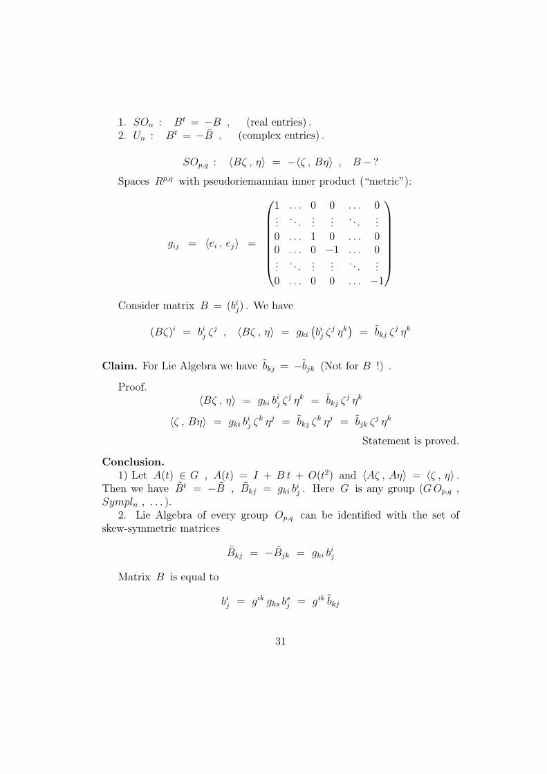
1. SOn : Bt = −B , (real entries) .2. Un : Bt = −B , (complex entries) .
SOp,q : ⟨Bζ , η⟩ = −⟨ζ , Bη⟩ , B− ?
Spaces Rp,q with pseudoriemannian inner product (“metric”):
gij = ⟨ei , ej⟩ =
1 . . . 0 0 . . . 0...
. . ....
.... . .
...0 . . . 1 0 . . . 00 . . . 0 −1 . . . 0...
. . ....
.... . .
...0 . . . 0 0 . . . −1
Consider matrix B = (bij) . We have
(Bζ)i = bij ζj , ⟨Bζ , η⟩ = gki
(bij ζ
j ηk)
= bkj ζj ηk
Claim. For Lie Algebra we have bkj = −bjk (Not for B !) .
Proof.⟨Bζ , η⟩ = gki b
ij ζ
j ηk = bkj ζj ηk
⟨ζ , Bη⟩ = gki bij ζ
k ηj = bkj ζk ηj = bjk ζ
j ηk
Statement is proved.
Conclusion.1) Let A(t) ∈ G , A(t) = I + B t + O(t2) and ⟨Aζ , Aη⟩ = ⟨ζ , η⟩ .
Then we have Bt = −B , Bkj = gki bij . Here G is any group (GOp,q ,
Sympln , . . . ).2. Lie Algebra of every group Op,q can be identified with the set of
skew-symmetric matrices
Bkj = −Bjk = gki bij
Matrix B is equal to
bij = gik gks bsj = gik bkj
31
with definition (gik)
= (gki)−1
General definition
Let Riemannian (pseudoriemannian) manifold Mn be given with Atlas
of Charts Uα, (x1α, . . . , xnα) and “metric” g
(α)ij (x) in the domain Uα. For 2
tangent vectors attached to x we have
⟨τ , η⟩ = gij(x) τi ηj
We define “metric” in the space of covectors ξ = (ξi), κ = (κj)
⟨ξ , κ⟩ = gij(x) ξi κj
where (gij) = (gkl)−1, i.e. gij gjk = δik .
Conclusion. T ∗(Mn) ∼= T∗(Mn) .
Remark. “Skew” metrics
gij(x) = − gij(x)
can be nondegenerate only for n = 2k (n even). We have here ⟨η , η⟩ ≡ 0 .
Gradient vector fieldLet function f : Mn → R be given. Its gradient is:
vector : ∇gf(x) =
(gij(x)
∂f
∂xj
)
covector : d f =
(∂f
∂xi
)Gradient system is
xi = gij∂f
∂xj= ηi(x)
Lemma. Let h(x) be any function in Mn. We have
dh
dt= ηi(x)
∂h
∂xi= ⟨∇gh , ∇gf⟩
32
Proof.
dh
dt= ηi(x)
∂h
∂xi= gij(x)
∂h
∂xi∂f
∂xj= ⟨dh , df⟩ = ⟨∇gh , ∇gf⟩
Lemma is proved.
Corollary 1.
gij = − gji ⇒ df
dt≡ 0
(Symplectic case).
Corollary 2. For Riemannian metric gij ηi ηj > 0 we have df/dt > 0
along the gradient system
xi = gij∂f
∂xj
(because (gij) = (gij)−1) .
Important example of Symplectic Manifold is T∗(Mn)
dim T∗(Mn) = 2n , Atlas : Uα , (x1α, . . . , xnα, pα1 , . . . , pαn)
Fix α - number of Chart.
Tangent basis : e′i =∂
∂xi, e′′i =
∂
∂pi
Inner Product is
⟨e′i , e′j⟩ = 0 , ⟨e′′i , e′′j ⟩ = 0 , ⟨e′i , e′′j ⟩ = −⟨e′′j , e′i⟩ = δij
τ = (e′i) - tangent vector to Mn, p = (e′′j ) - tangent covector to Mn,⟨τ , p⟩ = τ i pi - natural Invariant Inner Product.
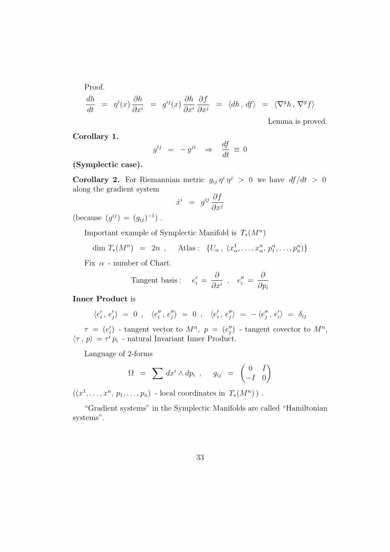
Language of 2-forms
Ω =∑
dxi ∧ dpi , gij =
(0 I−I 0
)((x1, . . . , xn, p1, . . . , pn) - local coordinates in T∗(M
n) ) .
“Gradient systems” in the Symplectic Manifolds are called “Hamiltoniansystems”.
33
Homework 2.
1. How many projection local coordinate systems for Sn ∈ Rn+1 are neededto cover all sphere? n = 1, 2, 3, . . . .
2. How many local coordinate systems are needed to cover RPn ? Letn = 1, 2, 3 .
x ∈ RPn =(Rn+1\0
)/x ∼ λx , λ = 0
(x0, . . . , xn) ∼ (λx0, . . . , λxn) , λ = 0
3. Prove that SO2 = U1 = S1 and SO3 = RP3 = S3/± 1 .
4. Which matrices belong to the Lie Algebra of the group SO2,1 ?
5. Find the group O1,1 . How many components does it have?
6. Prove that SO3 = SU2/± 1 .
7. Prove that SO4 = S3 × S3/± (1, 1) .
8. Prove that GL2(R) has 2 components. Same for On .
Lecture 8. Riemannian, Pseudo-Riemannian
and Symplectic Geometries.Complex Geom-
etry. Restriction of Metric to submanifolds.
Length of curves and Fermat Principle.
I. Riemannian Geometry = Manifold + Riemannian Metric gij ,gij η
i ηj > 0 .
II. Pseudoriemannian Geometry = Manifold + Pseudoriemannian Metricgij , det gij(x) = 0 .
III. Symplectic Geometry = Manifold + Symplectic Inner Product gij(x) =− gji(x) , det gij(x) = 0 . Corollary: dimM = 2k .
Main Example (Physics) = T∗(Mn) .
Flat Geometry:Mn = Rn , gij = const
34
1. Riemannian Case: ||η||2g > 0 , ⟨ei , ej⟩ = δij .
2. Pseudoriemannian Case: type p, q , ⟨ei , ej⟩ = ±δij .
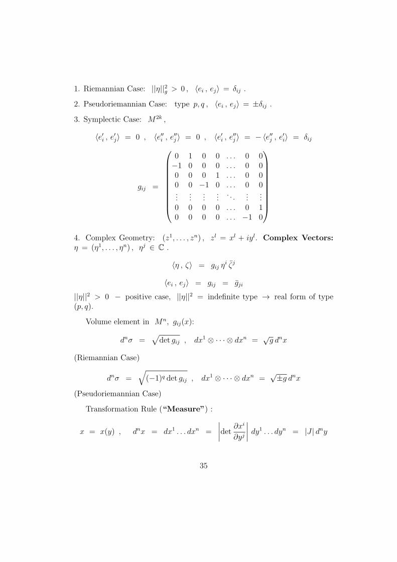
3. Symplectic Case: M2k ,
⟨e′i , e′j⟩ = 0 , ⟨e′′i , e′′j ⟩ = 0 , ⟨e′i , e′′j ⟩ = −⟨e′′j , e′i⟩ = δij
gij =
0 1 0 0 . . . 0 0−1 0 0 0 . . . 0 00 0 0 1 . . . 0 00 0 −1 0 . . . 0 0...
......
.... . .
......
0 0 0 0 . . . 0 10 0 0 0 . . . −1 0
4. Complex Geometry: (z1, . . . , zn) , zl = xl + iyl. Complex Vectors:η = (η1, . . . , ηn) , ηj ∈ C .
⟨η , ζ⟩ = gij ηi ζj
⟨ei , ej⟩ = gij = gji
||η||2 > 0 − positive case, ||η||2 = indefinite type → real form of type(p, q).
Volume element in Mn, gij(x):
dnσ =√
det gij , dx1 ⊗ · · · ⊗ dxn =√g dnx
(Riemannian Case)
dnσ =√(−1)q det gij , dx1 ⊗ · · · ⊗ dxn =
ñg dnx
(Pseudoriemannian Case)
Transformation Rule (“Measure”) :
x = x(y) , dnx = dx1 . . . dxn =
∣∣∣∣det ∂xi∂yj
∣∣∣∣ dy1 . . . dyn = |J | dny
35
Important Remark. For manifolds given by Oriented Atlas (J > 0)we can write dnx = J dny (differential forms !), J = det ||∂xi/∂yj|| .
Lemma 1. Riemannian Metric in the manifold Mn defines RiemannianMetric in every submanifold W k ⊂ Mn .
Proof.Let W k ⊂ Mn , locally we have for local coordinates y in Mn : yi =
yi(x1, . . . , xk) , i = 1, . . . , n, where x represent some local coordinates inW k.
We define “restriction of metric”
g′ij(x) = gsk(y(x))∂ys
∂xi∂yk
∂xj
(restriction of inner product on every linear subspace of tangent space). Itremains positive.
Lemma is proved.
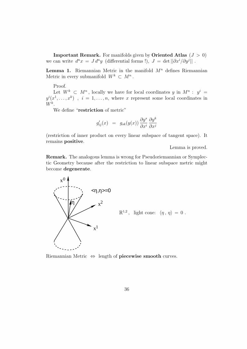
Remark. The analogous lemma is wrong for Pseudoriemannian or Symplec-tic Geometry because after the restriction to linear subspace metric mightbecome degenerate.
x0
x2
x1
<η,η>=0
η
R1,2 , light cone: ⟨η , η⟩ = 0 .
Riemannian Metric ⇔ length of piecewise smooth curves.
36
A
Bx(t)
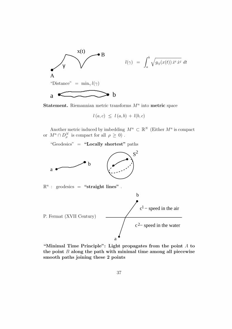
γl(γ) =
∫ b
a
√gij(x(t)) xi xj dt
“Distance” = minγ l(γ)
a b
Statement. Riemannian metric transforms Mn into metric space
l (a, c) ≤ l (a, b) + l(b, c)
Another metric induced by imbedding Mn ⊂ RN (EitherMn is compactor Mn ∩DN
ρ is compact for all ρ ≥ 0) .
“Geodesics” = “Locally shortest” paths
S2
ab
Rn : geodesics = “straight lines” .
P. Fermat (XVII Century)
a
b
c − speed in the air1
c − speed in the water2
“Minimal Time Principle”: Light propagates from the point A tothe point B along the path with minimal time among all piecewisesmooth paths joining these 2 points
37
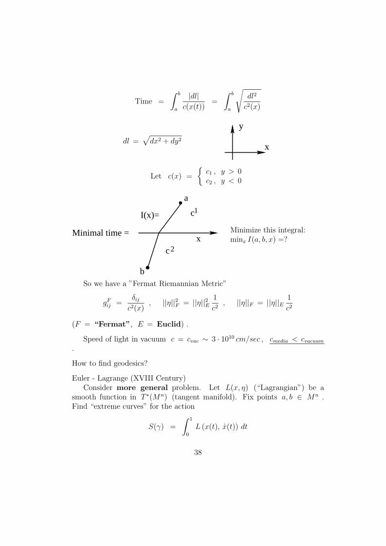
Time =
∫ b
a
|dl|c(x(t))
=
∫ b
a
√dl2
c2(x)
dl =√dx2 + dy2
y
x
Let c(x) =
c1 , y > 0c2 , y < 0
c2
c1
x
b
a
Minimal time =
I(x)=
Minimize this integral:minx I(a, b, x) =?
So we have a ”Fermat Riemannian Metric”
gFij =δijc2(x)
, ||η||2F = ||η||2E1
c2, ||η||F = ||η||E
1
c2
(F = “Fermat”, E = Euclid) .
Speed of light in vacuum c = cvac ∼ 3 · 1010 cm/sec , cmedia < cvacuum.
How to find geodesics?
Euler - Lagrange (XVIII Century)Consider more general problem. Let L(x, η) (“Lagrangian”) be a
smooth function in T ∗(Mn) (tangent manifold). Fix points a, b ∈ Mn .Find “extreme curves” for the action
S(γ) =
∫ 1
0
L (x(t), x(t)) dt
38
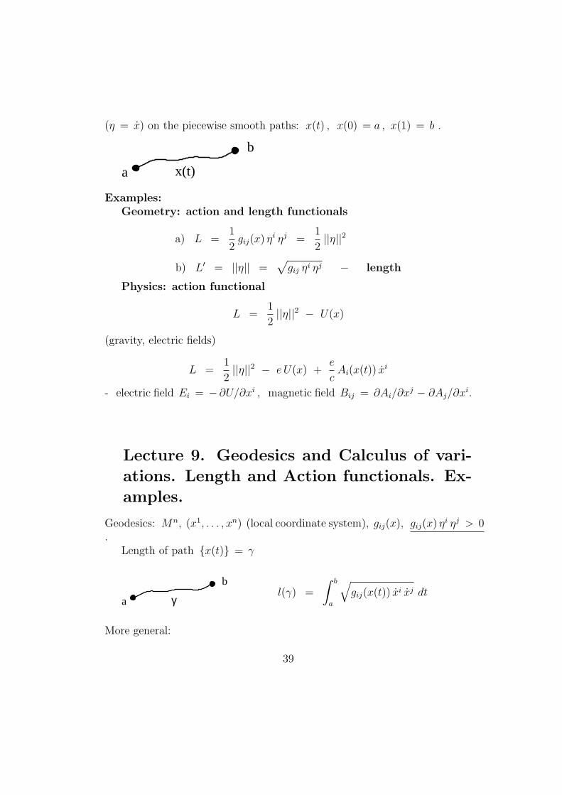
(η = x) on the piecewise smooth paths: x(t) , x(0) = a , x(1) = b .
a
b
x(t)
Examples:Geometry: action and length functionals
a) L =1
2gij(x) η
i ηj =1
2||η||2
b) L′ = ||η|| =√gij ηi ηj − length
Physics: action functional
L =1
2||η||2 − U(x)
(gravity, electric fields)
L =1
2||η||2 − eU(x) +
e
cAi(x(t)) x
i
- electric field Ei = − ∂U/∂xi , magnetic field Bij = ∂Ai/∂xj − ∂Aj/∂xi.
Lecture 9. Geodesics and Calculus of vari-
ations. Length and Action functionals. Ex-
amples.
Geodesics: Mn, (x1, . . . , xn) (local coordinate system), gij(x), gij(x) ηi ηj > 0
.Length of path x(t) = γ
a
b
γl(γ) =
∫ b
a
√gij(x(t)) xi xj dt
More general:
39
“Lagrangian” L(x, η) : T ∗(Mn) → R is given.“Action functional” is given
Sγ =
∫γ
L (x(t), x(t)) dt
Examples:
1) L = gij(x) xi xj/2 = ||x||2/2
2) L′ =√gij xi xj = ||x||
3) L′′ = ||x||2/2 − U(x) (gravity or electricity)
4) L′′′ = ||x||2/2 + (e/c)Ai(x) xi - magnetic field (its vector-potential).
5) “Relativistic Particle” (?)
Geodesics: Either (1) or (2)
P. Fermat: gij(x) = δij/c2(x)
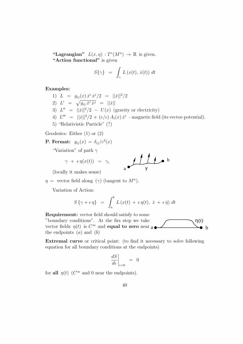
“Variation” of path γ
γ + ϵ η(x(t)) = γϵ
(locally it makes sense)a
b
γ
η = vector field along (γ) (tangent to Mn).
Variation of Action:
S γ + ϵ η =
∫ b
a
L (x(t) + ϵ η(t), x + ϵ η) dt
Requirement: vector field should satisfy to some”boundary conditions”. At the firs step we takevector fields η(t) is C∞ and equal to zero nearthe endpoints (a) and (b)
baη(t)
Extremal curve or critical point: (to find it necessary to solve followingequation for all boundary conditions at the endpoints)
dS
dϵ
∣∣∣∣ϵ=0
= 0
for all η(t) (C∞ and 0 near the endpoints).
40
Lemma (Euler - Lagrange).Curve γ is extremal iff
d
dt
(∂L
∂xi
)=
∂L
∂xi,
L = L(x, x) , (x, x) ∈ T ∗(Mn) .
Proof. We have
dS
dϵ(γ + ϵ η)
∣∣∣∣ϵ=0
=d
dϵ
∫ b
a
L (x(t) + ϵ η(t), x + ϵ η) dt =
=
∫ b
a
(∂L
∂xiηi +
∂L
∂xiηi)dt =
∫ b
a
(∂L
∂xi− d
dt
∂L
∂xi
)ηi dt
which is true for all η(t) which are C∞ and equal to zero near a and b .Indeed, we have∫ b
a
∂L
∂xiηi dt = −
∫ b
a
ηid
dt
∂L
∂xidt +
(ηi∂L
∂xi
)∣∣∣∣ba
= −∫ b
a
ηid
dt
∂L
∂xidt
because ηi(a) = ηi(b) = 0 .
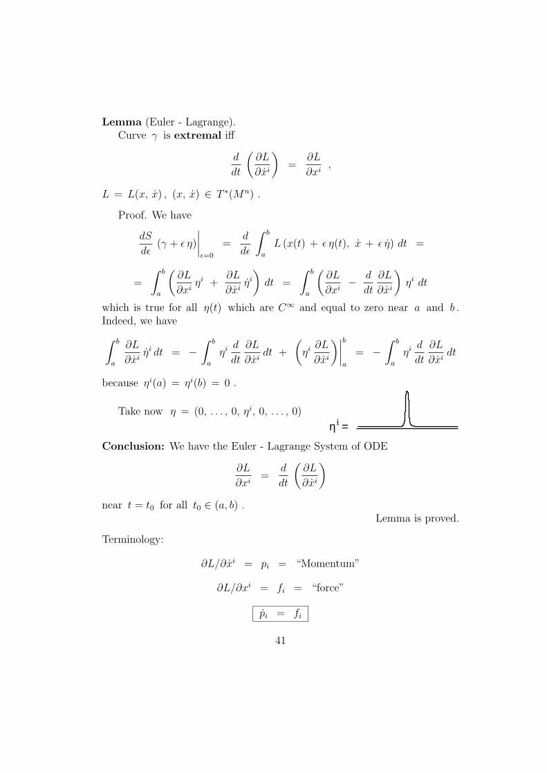
Take now η = (0, . . . , 0, ηi, 0, . . . , 0)
η =i
Conclusion: We have the Euler - Lagrange System of ODE
∂L
∂xi=
d
dt
(∂L
∂xi
)near t = t0 for all t0 ∈ (a, b) .
Lemma is proved.
Terminology:
∂L/∂xi = pi = “Momentum”
∂L/∂xi = fi = “force”
pi = fi
41
L =1
2gij(x) x
i xj ⇒ pi = gij xj
T ∗(Mn) → T∗(Mn)
x → pvelocity momentumvector (covector)
Equation of Geodesics:
pk =∂L
∂xk=
1
2
(∂gij∂xk
)xi xj
Another form (for length) L′ =√gij xi xj :
d
dt
(pk√
gij(x) xi xj
)=
∂L′
∂xk=
1
2√gij(x) xi xj
∂gij∂xk
xi xj
Conclusion. Let parameter t for the length functional L′ is “natural”, i.e.t = l(γ) (length), dt =
√gij(x(t)) xi xj . Then we have same equations
for both L and L′ because√gij(x(t)) xi xj = 1 .
Corollaries.1) Geodesics for Rn , gij = δij , are thestraight lines. a
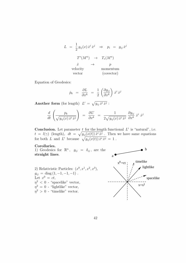
b
2) Relativistic Particles: (x0, x1, x2, x3),gij = diag (1,−1,−1,−1) .Let x0 = ct,η2 < 0 - “spacelike” vector,η2 = 0 - “lightlike” vector,η2 > 0 - “timelike” vector.
lightlike
spacelike
timelike
x=x
x =ct0
1
42
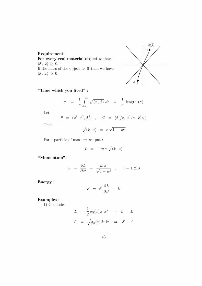
Requirement:For every real material object we have:⟨x , x⟩ ≥ 0.If the mass of the object > 0 then we have:⟨x , x⟩ > 0 .
x(t)
a
b
“Time which you lived” :
τ =1
c
∫ b
a
√⟨x , x⟩ dt =
1
clength (γ)
Letv = (x1, x2, x3) , w = (x1/c, x2/c, x3/c)
Then √⟨x , x⟩ = c
√1 − w2
For a particle of mass m we put :
L = −mc√⟨x , x⟩
“Momentum”:
pi =∂L
∂xi=
mxi√1− w2
, i = 1, 2, 3
Energy :
E = xi∂L
∂xi− L
Examples :1) Geodesics
L =1
2gij(x) x
i xj ⇒ E = L
L′ =√gij(x) xi xj ⇒ E ≡ 0
43
2) Gravity or electric field
L′′ =1
2gij(x) x
i xj − U(x) ⇒ E =1
2gij(x) x
i xj + U(x)
3) Magnetic field
L′′′ =1
2gij(x) x
i xj +e
cAi(x) x
i ⇒ E =1
2gij(x) x
i xj
Equations :1) Geodesics
pk =1
2
(∂gij∂xk
)xi xj , pk = gkj x
j
2) Gravity or electric field
pk −1
2
(∂gij∂xk
)xi xj = − ∂U
∂xk, pk = gkj x
j
3) Magnetic field
pk −1
2
(∂gij∂xk
)xi xj =
e
c
∂Ai∂xk
xi , pk = gkj xj +
e
cAk(x)
i.e.d
dt
(gkj x
j)− 1
2
(∂gij∂xk
)xi xj =
e
c
(∂Ai∂xk
− ∂Ak∂xi
)xi
Magnetic field
Bik =∂Ai∂xk
− ∂Ak∂xi
Lecture 10. Variational problem and geodesics
on Riemannian manifolds: Action Functional,
Lagrangian, Energy, Momentum. Conserva-
tion of Energy and Momentum.
Mn, (x1, . . . , xn) , gij(x) .
44
“Lagrangian”: L(x, η) : T ∗(Mn) → R .
Sγ =
∫γ
L (x(t), x(t)) dt (Action)
“Momentum”: pi = ∂L/∂xi = ∂L/∂vi
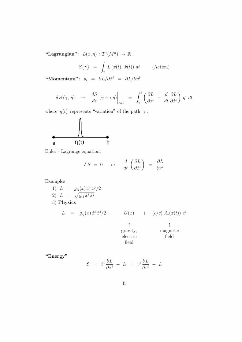
δ S (γ, η) → dS
dϵ(γ + ϵ η)
∣∣∣∣ϵ=0
=
∫ b
a
(∂L
∂xi− d
dt
∂L
∂xi
)ηi dt
where η(t) represents “variation” of the path γ .
a bη(t)
Euler - Lagrange equation:
δ S = 0 ↔ d
dt
(∂L
∂xi
)=
∂L
∂xi
Examples
1) L = gij(x) xi xj/2
2) L =√gij xi xj
3) Physics
L = gij(x) xi xj/2 − U(x) + (e/c) Ai(x(t)) x
i
↑ ↑gravity, magneticelectric fieldfield
“Energy”
E = xi∂L
∂xi− L = vi
∂L
∂vi− L
45
Energy Conservation Law
Theorem 10.1. For the Euler - Lagrange System we have the followingconservation law:
dEdt
= 0
(i.e. E is constant along the trajectories of the Euler - Lagrange System).
Proof.
dEdt
=d
dt
(xi∂L
∂xi− L
)= xi
∂L
∂xi+ xi
d
dt
(∂L
∂xi
)− ∂L
∂xixi − ∂L
∂xixi =
=
[d
dt
(∂L
∂xi
)− ∂L
∂xi
]xi = 0
Theorem is proved.
Momentum Conservation Law
Theorem 10.2. Let L(x, v) does not depend on x1 :
L = L (x2, . . . , xn, v1, . . . , vn)
Then we have: p1 = 0 on the trajectories of the Euler - Lagrange System.
Proof.
p1 =d
dt
(∂L
∂x1
)=
∂L
∂x1= 0
Theorem is proved.
Definition. Vector field ζ = (ζ i(y)) is called “Symmetry” of Lagrangianif L(x, v) does not depend on x1 in the local coordinate system (x) whereζ = (1, 0, . . . , 0) .
Corollary. In the original system (y1, . . . , yn) we have ζ = (ζ1, . . . , ζn)The component pζ = pi ζ
i is a conservative quantity pζ = 0 because pζ
is exactly the first component of p in the system (x1, . . . , xn) where ζ =(1, 0, . . . , 0) .
46
Examples.
1) L = gij(x) xi xj/2
Energy
E = xi∂L
∂xi− L = L
E = 0 ⇒ - parameter along geodesics is NATURAL because
E =1
2||x||2g = const
along trajectory.
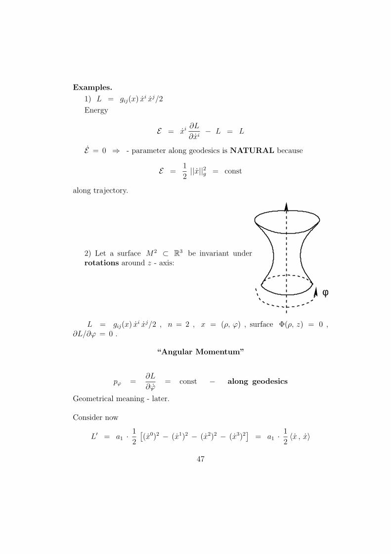
2) Let a surface M2 ⊂ R3 be invariant underrotations around z - axis:
φ
L = gij(x) xi xj/2 , n = 2 , x = (ρ, φ) , surface Φ(ρ, z) = 0 ,
∂L/∂φ = 0 .
“Angular Momentum”
pφ =∂L
∂φ= const − along geodesics
Geometrical meaning - later.
Consider now
L′ = a1 ·1
2
[(x0)2 − (x1)2 − (x2)2 − (x3)2
]= a1 ·
1
2⟨x , x⟩
47
L′′ = a2 ·√
(x0)2 − (x1)2 − (x2)2 − (x3)2 = a2 ·√⟨x , x⟩ , t = x0/c
Relativity
Use L′ : E ′ = L′ , p(4)i =
∂L′
∂xi
time τ ∼ length by theorem above so
p(4)i =
∂L′
∂xi= a1 ·
(dx0
dt
dt
dτ, − dx
1
dt
dt
dτ, . . . , − dx
3
dt
dt
dτ
)dt
dτ= 1 /
dτ
dt=
1√c2 −
∑3α=1 (v
α)2=
1√c2 − v2
where
v =
(dx1
dt,dx2
dt,dx3
dt
)4-D Formalism
So we have for the 4-momentum
p(4) = a1 ·(
1√1− w2
, − dx1/dt
c√1− w2
, − dx2/dt
c√1− w2
, − dx3/dt
c√1− w2
)where w = v/c .
Clearly we have to choose: a1 = mc , where m is the mass of aparticle.
3-D Formalism
Use L′′ . We use time t = x0/c , x0 = ct .
L′′ = a2 ·√
(c2 − (x1)2 − (x2)2 − (x3)2
p(3)α =∂L′′
∂xα= − a2 ·
vα√c2 − v2
= − a2c
vα√1− v2/c2
vα = dxα/dt , α = 1, . . . , 3 . We choose a2 = −mc .So we finally have
E ′′ = xα∂L′′
∂xα− L′′ =
mc2√1− w2
, w = v/c
48
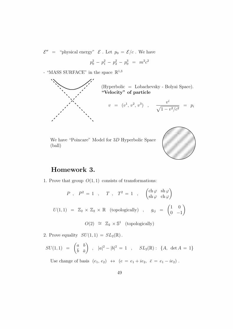
E ′′ = “physical energy” E . Let p0 = E/c . We have
p20 − p21 − p22 − p30 = m2c2
- “MASS SURFACE” in the space R1,3
(Hyperbolic = Lobachevsky - Bolyai Space).“Velocity” of particle
v = (v1, v2, v3) ,vi√
1− v2/c2= pi
We have “Poincare” Model for 3D Hyperbolic Space(ball)
Homework 3.
1. Prove that group O(1, 1) consists of transformations:
P , P 2 = 1 , T , T 2 = 1 ,
(chφ shφshφ chφ
)
U(1, 1) = Z2 × Z2 × R (topologically) , gij =
(1 00 −1
)O(2) ∼= Z2 × S1 (topologically)
2. Prove equality SU(1, 1) = SL2(R) .
SU(1, 1) =
(a bb a
), |a|2 − |b|2 = 1 , SL2(R) : A, detA = 1
Use change of basis (e1, e2) ↔ (e = e1 + ie2, e = e1 − ie2) .
49
3. Prove that SL2(R) ∼= R2 × S1 (topologically).
4. Calculate Euclidean Riemannian metric of R2 in polar coordinates.
5. Calculate Riemannian Metric of sphere S2 :
S2 : x2 + y2 + z2 = 1 , R3 : dl2 = dx2 + dy2 + dz2
in the spherical coordinates θ, φ :
z = r cosφ , x = r sin θ cosφ , y = r sin θ sinφ , (r = 1)
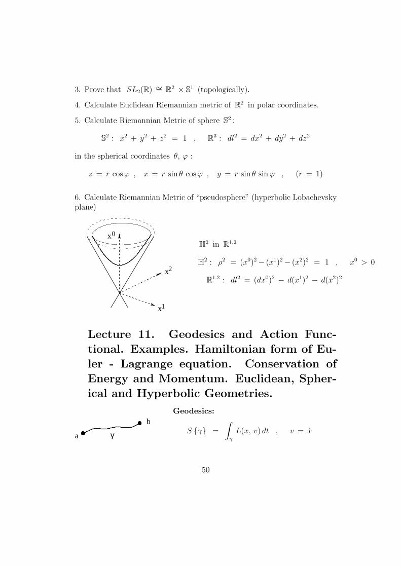
6. Calculate Riemannian Metric of “pseudosphere” (hyperbolic Lobachevskyplane)
x0
x2
x1
H2 in R1,2
H2 : ρ2 = (x0)2− (x1)2− (x2)2 = 1 , x0 > 0
R1.2 : dl2 = (dx0)2 − d(x1)2 − d(x2)2
Lecture 11. Geodesics and Action Func-
tional. Examples. Hamiltonian form of Eu-
ler - Lagrange equation. Conservation of
Energy and Momentum. Euclidean, Spher-
ical and Hyperbolic Geometries.
a
b
γ
Geodesics:
S γ =
∫γ
L(x, v) dt , v = x
50
L =1
2gij(x) x
i xj , L(x, η) : T ∗(Mn) → R
Euler - Lagrange Equations:
pi =∂L
∂vi, pi = gij v
j
gij(x) xj +
∂gij∂xk
xk xj =1
2
∂gjk∂xi
xk xj
xj gij =
(1
2
∂gjk∂xi
− ∂gij∂xk
)xk xj
xp = gpi(1
2
∂gjk∂xi
− ∂gij∂xk
)xk xj
Let us introduce the “Christoffel Symbols”
Γpkj = Γpjk =1
2gpi(∂gij∂xk
+∂gik∂xj
− ∂gjk∂xi
)We have then
xp + Γpkj xk xj = 0
Euclidean (Pseudoriemannian) Metric: Γpkj = 0 .
Examples:
1. R2 : dx2 + dy2 ⇒ dz dz = dr2 + r2(dφ)2
2. S2 : dθ2 + sin2θ dφ2 ⇒ dz dz
(1 + |z|2)2
3. H2 : dχ2 + sh2χdφ2 ⇒ dz dz
(1− |z|2)2⇒ dz dz
y2
Lemma 1. For the general metric of the form dl2 = dρ2 + Φ2(ρ) (dφ)2
every line φ = const is geodesics.Proof. We have
L =1
2
(ρ2 + Φ2(ρ) φ2
)51
Euler - Lagrange equations:
ρ = ΦΦ′(ρ) φ2 ,d
dt
(Φ2(ρ) φ
)= 0
So we have: φ = 0 always satisfy to the Euler - Lagrange equations.Lemma is proved.
Remark. Integrate Euler - Lagrange equations now:
Φ2 φ = a = const ⇒ φ = a/Φ2(ρ)
and therefore: ρ = ΦΦ′(ρ) a2/Φ4(ρ) = a2Φ′(ρ)/Φ3(ρ) ,
so : ρ = − a2 ∂V (ρ)
∂ρ, V (ρ) =
1
2Φ2(ρ),
so : ρ ρ + a2∂V (ρ)
∂ρρ or
ρ2
2+
a2
Φ2(ρ)= b = const
We have thenρ =
√2(a2/Φ2(ρ)− b)
and
t =
∫dρ√
2(a2/Φ2(ρ)− b)⇒ ρ = ρ(t) , φ = a/Φ2(ρ)
Conclusion. Every geodesics for the M2 = R2, S2, H2 can be obtainedfrom the straight line φ = 0 (or φ = const) by the action of the followinggroups:
1) R2 : Iso (R2) − straight lines (Euclidean space).
2) S2 : SO3 − big circles (round sphere).
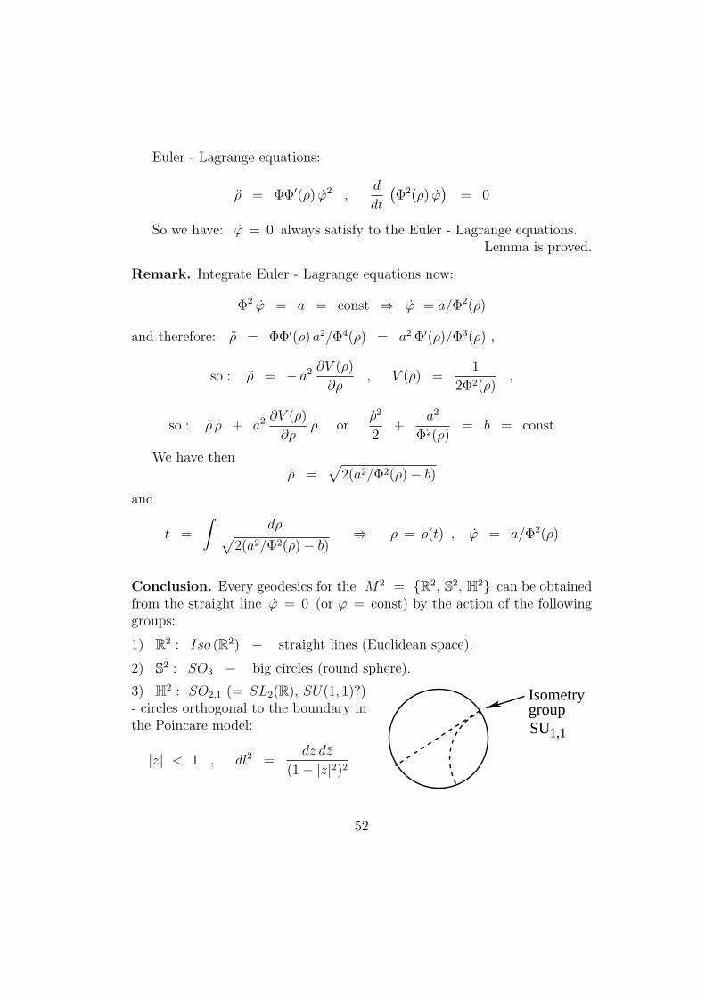
3) H2 : SO2,1 (= SL2(R), SU(1, 1)?)- circles orthogonal to the boundary inthe Poincare model:
|z| < 1 , dl2 =dz dz
(1− |z|2)2
SU1,1
Isometrygroup
52
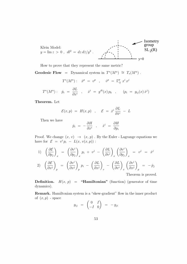
Klein Model:y = Im z > 0 , dl2 = dz dz/y2 .
SL (R)2
y=0
Isometrygroup
How to prove that they represent the same metric?
Geodesic Flow = Dynamical system in T ∗(Mn) ∼= T∗(Mn) .
T ∗(Mn) : xp = vp , vp = Γpij xi xj
T ∗(Mn) : pi =∂L
∂xi, xi = gik(x) pk , (pi = gij(x) x
j)
Theorem. Let
E(x, p) = H(x, p) , E = xi∂L
∂xi− L
Then we have
pi = − ∂H∂xi
, xi =∂H
∂pi
Proof. We change (x, v) → (x, p) . By the Euler - Lagrange equations wehave for E = vi pi − L(x, v(x, p)) :
1)
(∂E∂pj
)x
=
(∂vi
∂pj
)x
pi + vj −(∂L
∂vi
)x
(∂vi
∂pj
)x
= vj = xj
2)
(∂E∂xj
)p
=
(∂vi
∂xj
)p
pi −(∂L
∂xj
)v
−(∂L
∂vi
)x
(∂vi
∂xj
)p
= − pj
Theorem is proved.
Definition. H(x, p) = “Hamiltonian” (function) (generator of timedynamics).
Remark. Hamiltonian system is a “skew-gradient” flow in the inner productof (x, p) - space
gij =
(0 I−I 0
)= − gji
53
2-form
Ω =n∑i=1
dxi ∧ dpi
is invariant under the flow (later).
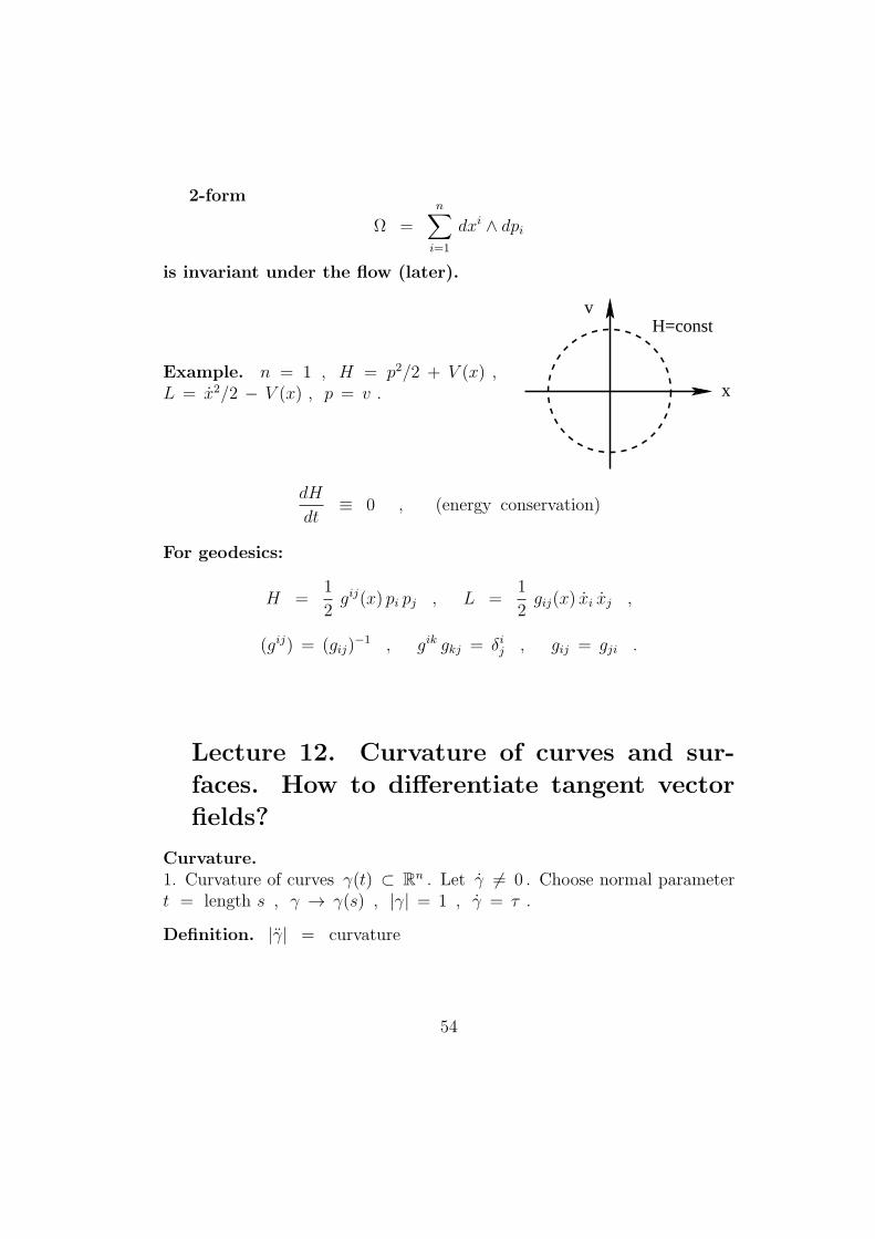
Example. n = 1 , H = p2/2 + V (x) ,L = x2/2 − V (x) , p = v . x
vH=const
dH
dt≡ 0 , (energy conservation)
For geodesics:
H =1
2gij(x) pi pj , L =
1
2gij(x) xi xj ,
(gij) = (gij)−1 , gik gkj = δij , gij = gji .
Lecture 12. Curvature of curves and sur-
faces. How to differentiate tangent vector
fields?
Curvature.1. Curvature of curves γ(t) ⊂ Rn . Let γ = 0 . Choose normal parametert = length s , γ → γ(s) , |γ| = 1 , γ = τ .
Definition. |γ| = curvature
54
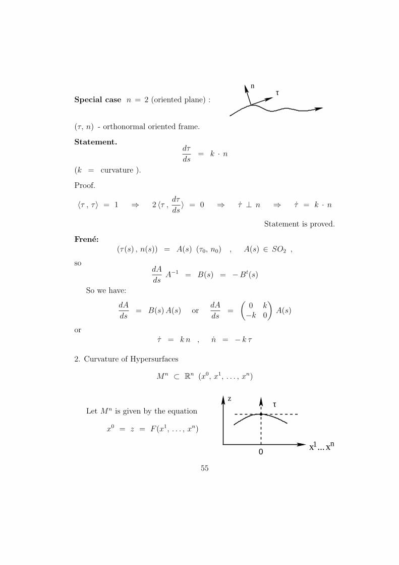
Special case n = 2 (oriented plane) :
nτ
(τ, n) - orthonormal oriented frame.
Statement.dτ
ds= k · n
(k = curvature ).
Proof.
⟨τ , τ⟩ = 1 ⇒ 2 ⟨τ , dτds⟩ = 0 ⇒ τ ⊥ n ⇒ τ = k · n
Statement is proved.
Frene:(τ(s) , n(s)) = A(s) (τ0, n0) , A(s) ∈ SO2 ,
sodA
dsA−1 = B(s) = −Bt(s)
So we have:
dA
ds= B(s)A(s) or
dA
ds=
(0 k−k 0
)A(s)
orτ = k n , n = − k τ
2. Curvature of Hypersurfaces
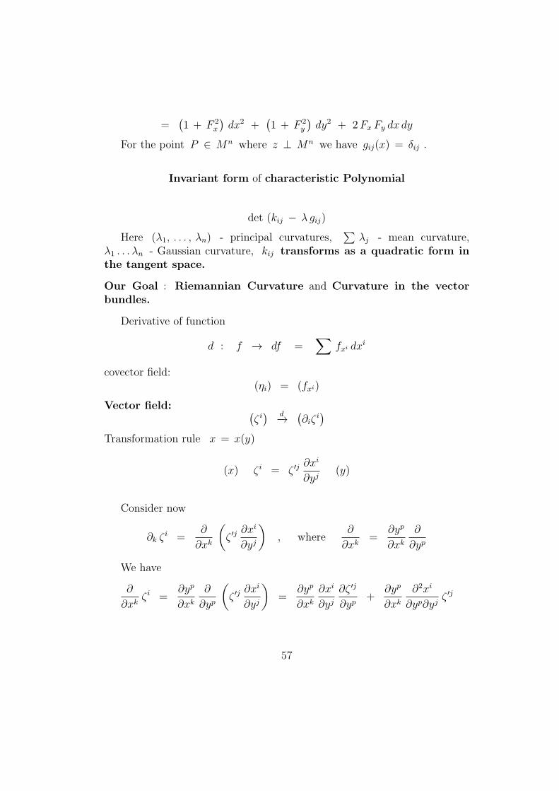
Mn ⊂ Rn (x0, x1, . . . , xn)
Let Mn is given by the equation
x0 = z = F (x1, . . . , xn)
1x xn
z
0
τ
...
55
Coordinate system is chosen in such a way that z ⊥ Mn at the pointP : (x1, . . . , xn) = (0, . . . , 0) , so we have near P :
∂z
∂xj
∣∣∣∣P
=∂F
∂xj
∣∣∣∣(0,...,0)
= 0 , j = 1, . . . , n
Curvature form (“Second quadratic form”) kij dxi dxj :
kij dxi dxj =
∂2F
∂xi∂xjdxi dxj
(at P only!)It describes curvature of Normal Sections (curves) in Rn+1 , n ≥ 2 .
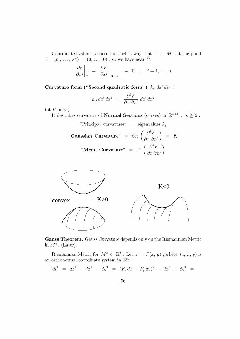
′′Principal curvatures′′ = eigenvalues kj
′′Gaussian Curvature′′ = det
(∂2F
∂xi∂xj
)= K
′′Mean Curvature′′ = Tr
(∂2F
∂xi∂xj
)
K>0convex
K<0
Gauss Theorem. Gauss Curvature depends only on the Riemannian Metricin Mn. (Later).
Riemannian Metric for M2 ⊂ R3 . Let z = F (x, y) , where (z, x, y) isan orthonormal coordinate system in R3.
dl2 = dz2 + dx2 + dy2 = (Fx dx + Fy dy)2 + dx2 + dy2 =
56
=(1 + F 2
x
)dx2 +
(1 + F 2
y
)dy2 + 2Fx Fy dx dy
For the point P ∈ Mn where z ⊥ Mn we have gij(x) = δij .
Invariant form of characteristic Polynomial
det (kij − λ gij)
Here (λ1, . . . , λn) - principal curvatures,∑
λj - mean curvature,λ1 . . . λn - Gaussian curvature, kij transforms as a quadratic form inthe tangent space.
Our Goal : Riemannian Curvature and Curvature in the vectorbundles.
Derivative of function
d : f → df =∑
fxi dxi
covector field:(ηi) = (fxi)
Vector field: (ζ i) d−→
(∂iζ
i)
Transformation rule x = x(y)
(x) ζ i = ζ ′j∂xi
∂yj(y)
Consider now
∂k ζi =
∂
∂xk
(ζ ′j
∂xi
∂yj
), where
∂
∂xk=
∂yp
∂xk∂
∂yp
We have
∂
∂xkζ i =
∂yp
∂xk∂
∂yp
(ζ ′j
∂xi
∂yj
)=
∂yp
∂xk∂xi
∂yj∂ζ ′j
∂yp+
∂yp
∂xk∂2xi
∂yp∂yjζ ′j
57
Conclusion: Second derivative enters in the change of coordinates rule(∂
∂xkζ i)
=
(∂
∂ypζ ′j)∂yp
∂xk∂xi
∂yj+
∂2xi
∂yp∂yj∂yp
∂xkζ ′j
TENSOR LAW NONTENSOR LAW
For covectors:
∂
∂xk(ηi) =
∂yp
∂xk∂
∂yp
(η′j∂yj
∂xi
)=
(∂
∂ypη′j
)∂yp
∂xk∂yj
∂xi+
∂2yj
∂xk∂xiη′j
Conclusion 1. Skew symmetric expression ∂k ηi − ∂i ηk transforms as atensor (inner product)
(x) (∂k ηi − ∂i ηk) =(∂′p η
′q − ∂′q η
′p
) ∂yp∂xk
∂yq
∂xi(y) , x = x(y)
or
(x)∂xk
∂yp∂xi
∂yq(∂k ηi − ∂i ηk) = ∂′p η
′q − ∂′q η
′p
which makes sense even if number of (x)′s (n) is not equal to number of (y)′s(m) !
f :(y) → (x)
Nm → Mn
We call the corresponding tensor “differential 2-form”
hij(x) = −hji(x)
h′pq = hij∂xi
∂yp∂xq
∂yq, h → f ∗(h)
f ∗ :h′ ← h
2− form in Nm 2− form in Mn
Conclusion 2. Quantities ∂i ηj and ∂k ζp are not tensors. How to make
tensors?
58
“Covariant derivatives”
∇i ηj = ∂i η
j + Γjik ηk
∇i ηj = ∂i ηj − Γkij ηk
where Γijk are “Christoffel Symbols”.
Requirements: ∇i ηj and ∇i ηj are tensors.
Difficulty: ∇i∇j = ∇j∇i , ∇i∇j − ∇j∇i = Rij (“Curvature”).
More general (local picture): consider Ψ(x) ∈ RLx , where RL
x is a linearspace with basis (e1(x), . . . , eL(x)) depending on the point (x1, . . . , xn) ,Ψ(x) =
∑Ψi ei(x) . Consider the set of linear equations
∂Ψi/∂xj = Aijk Ψk (x1, . . . , xn)
Can we solve this system?
Let us define Operators of “Covariant Derivatives”
∇j =∂
∂xj− Aijk(x)
Lemma. The set of linear equations (above) is solvable for all “initialdata” Ψ(x0) = Ψ0 if and only if
∇i∇j − ∇j∇i = Rij = 0
for all x ∈ Rn .
Proof. For every solution Ψ(x) we have
∂iΨ = AiΨ (Ai = matrix)
and∂i ∂j Ψ = ∂i (Aj Ψ) = ∂j (AiΨ)
or(∂iAj − ∂j Ai) Ψ + Aj (∂iΨ) − Ai (∂j Ψ) = 0
or(∂iAj − ∂j Ai − AiAj + Aj Ai) Ψ = 0
59
where(∂iAj − ∂j Ai − AiAj + Aj Ai) = Rij (matrix)
So we have Rij Ψ = 0 for all x ∈ Rn . Therefore Rij ≡ 0 .Lemma is proved.
Rij = [∇i , ∇j]
Examples.
a) L = n , Ψ - vector field, Aijk = −Γijk .
b) L = n , Ψ - covector field, Aijk = Γijk .
c) L = 1 , Ai - scalar values, AiAj − Aj Ai = 0 ,
∂iAj − ∂j Ai = Rij
Lecture 13. Vector bundles. Connection
and Curvature. Parallel transport.
Vector bundles and Curvature.Vector bundle = Family of Linear Spaces RN
x depending on parameterx ∈ X and “locally trivial”:
For every point x ∈ X there exists an open set U ∋ x such that we canchoose a basis [eU1 (x), . . . , e
UN(x)] ∈ RN
x continuously depending on x ∈ X .For x ∈ U ∩ V we have
eUi (x) = aj UVi (x) eVj (x)
Real case: aij ∈ GLn(R)Complex case: aij ∈ GLn(C)Orthogonal case: aij ∈ On
Unitary case: aij ∈ Un
- For all pairs U , V (!).
60
Other groups are also possible and define the “structural group” of thebundle.
Our case: X is a C∞-manifold and aij(x) are C∞-functions.
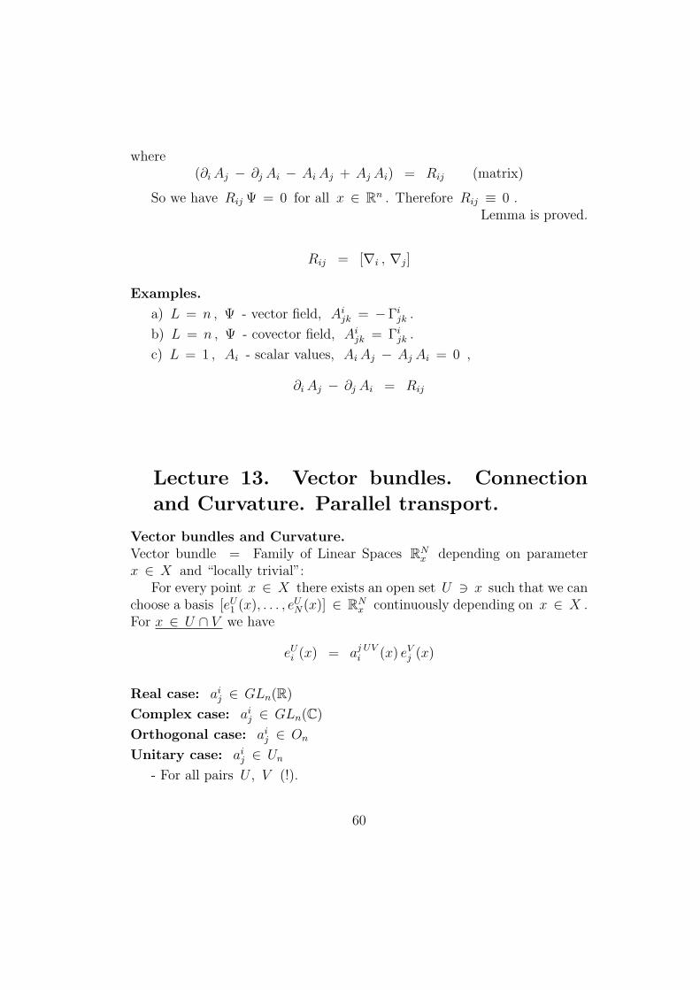
Example. Let X = Mk ⊂ RL . Considerfamily of tangent k-spaces to Mk.
Map G : Mk → Gk,L (Grassmann Manifold).
Curvature is local quantity.
Locally vector bundle is given by the product U × Rn according to thechoice of the basis e1(x), . . . , en(x) in Rn .
Consider set of linear ODE’s
∂Ψj
∂xi= Ajip(x) Ψ
p(x) , Ψ =∑
Ψj(x) ej
i = 1, . . . , n , j, p = 1, . . . , N .or:
∇iΨj = ∂iΨ
j − AjipΨp = 0
Is this system solvable?
For n = 1 it is true.
For n > 1 it may be wrong! “Curvature” Rij of this “Differen-tial Geometric Connection” Ajip(x) should be equal to zero:
[∇i , ∇q] = ∇i∇q − ∇q∇i =
[∂
∂xi− Ajip(x) ,
∂
∂xq− Ajql(x)
]= 0
As we saw in the previous lecture, we can formulate the following Lemma:
Lemma. The set of linear equations (above) is solvable for all “initialdata” Ψ(x0) = Ψ0 if and only if
∇i∇j − ∇j∇i = Rij = 0
61
for all x ∈ Rn .
Rij = [∇i , ∇j]
Examples.
a) L = n , Ψ - vector field, Aijk = −Γijk .
b) L = n , Ψ - covector field, Aijk = Γijk .
c) L = 1 , Ai - scalar values, AiAj − Aj Ai = 0 ,
∂iAj − ∂j Ai = Rij
“Gauge Transformations”, CurvatureWe have ∂iΨ = AiΨ (Matrix Form), Ai = Akij(x) , so
∇i = ∂i − Ai , ∇q = ∂q − Aq ,
[∇i , ∇q] = Riq = − ∂Aq∂xi
+∂Ai∂xq
+ AiAq − Aq Ai
(Matrices in RN) .
1) For tangent (cotangent) case N = n .
2) For scalar case N = 1 , n is any.
3) For euclidean case ⟨ei , ej⟩ = δij we should have (Ai)kj = − (Ai)
jk
(skew symmetry).
Change of Basis:ei = bij(x) e
′j , [e = B e′]
orΨi ei = Ψi bji e
′j , Ψ′j = Ψi bji
Ψ′ = B(x) Ψ
Lemma 2. Let∂Ψj
∂xi= Ajik Ψk(x)
62
Then for the new basis (e′j) we have
∂Ψ′j
∂xi= A′j
ik Ψ′k(x)
where
A′i = BAiB
−1 +∂B
∂xiB−1
Proof. We have Ψ′ = B(x)Ψ , so
∂Ψ′j
∂xi= BAiΨ +
∂B
∂xiΨ = BAiB
−1 Ψ′ +∂B
∂xiB−1Ψ′
Lemma is proved.
Conclusion.
A′i = BAiB
−1 +∂B
∂xiB−1
Let B−1 = G(x) , we have then
A′i = G−1AiG − G−1 ∂G
∂xi
- Gauge Transformation.
Homework 4.
1. Prove that the group O(1, 1) (connected component) can be written inthe form (
chψ shψshψ chψ
)=
(1√
1−w2
w√1−w2
w√1−w2
1√1−w2
)
2. a) Prove that every isometry of R2 , preserving orientation, is either shiftor rotation around some point.
b) Prove that every isometry of R2 , inverting orientation, is product ofreflection and shift along this line (line of reflection).
3. How many local coordinate systems are needed to cover RP2 ? Find coverby 3 domains.
63
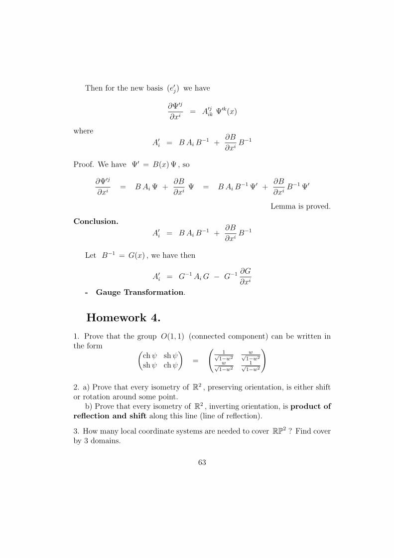
4. Find cover of sphere S2g with g handles by 2 systems of local coordinates.
S =g2
5. Introduce “pseudospherical” coordinates
x0 = ρ ch θ , x1 = ρ sh θ cosφ , x2 = ρ sh θ sinφ
Restrict metric(dx0)2 − (dx1)2 − (dx2)2
on the “pseudoshere” ρ = 1 . Calculate it.
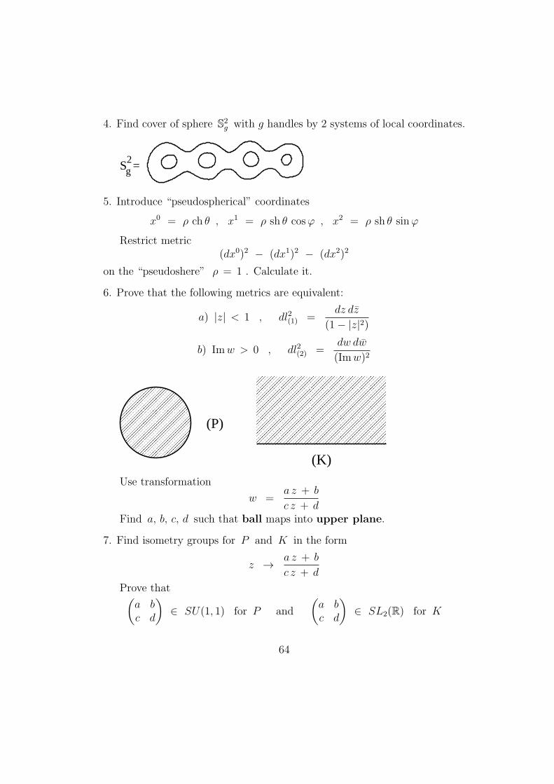
6. Prove that the following metrics are equivalent:
a) |z| < 1 , dl2(1) =dz dz
(1− |z|2)
b) Imw > 0 , dl2(2) =dw dw
(Imw)2
(P)
(K)
Use transformation
w =a z + b
c z + dFind a, b, c, d such that ball maps into upper plane.
7. Find isometry groups for P and K in the form
z → a z + b
c z + d
Prove that(a bc d
)∈ SU(1, 1) for P and
(a bc d
)∈ SL2(R) for K
64
Lecture 14. Vector bundles. Connection
and Curvature. Parallel transport.
Vector bundle=“locally trivial” family of vector spaces RNx , x ∈ X with
“local bases” [eU1 (x), . . . , eUN(x)], x ∈ U ⊂ X, ∀x ∃U ∋ x.
For x ∈ U ∩ VeUi (x) = aj,UVi (x)eNj (x).
“Group” aj,UVi (x) ∈ G ⊂ GLN(R)
Differential geometrical connection (on vector bundle).
Locally matrix-valued functions Ai(x) = (Ai)jk(x) are given for all x ∈
U ⊂ X, and operators ∇Ui = ∂i − AUi acting on functions ΨU : U → RN ,
ΨU = (Ψj,U),∇Ui Ψ
U = ∂iΨU − AUi ΨU .
In intersection x ∈ U ∩ V we have
ΨU = gUVΨV , G(x) = gUV (x),
such that:AVi = G−1(x)AUi G(x)−G−1∂iG
(gauge equivalence).
“Curvature”
RUij = ∇U
i ∇Uj −∇U
j ∇Ui (matrix functions).
Theorem (Later):RVij = G−1RU
ijG (!)
ξ-tangent vector to X =Mn in the point x ∈Mn, x1, . . . , xn.
∇Uξ =
(∂ΨU
∂xi− AiΨU
)ξi
– covariant derivative along ξ ∈ T ∗X .
Curve γ = xi(t). Covariant derivative along γ:
65
γ(t)ix (t)x 0
∇Uγ = ∇U
x(t) = xi∇Ui Ψ
U .
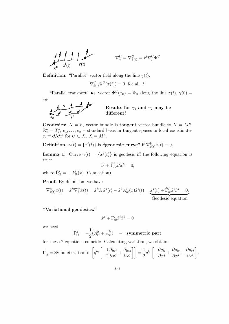
Definition. “Parallel” vector field along the line γ(t):
∇Ux(t)Ψ
U(x(t)) ≡ 0 for all t.
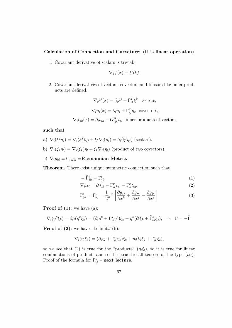
“Parallel transport” •+ vector ΨU(x0) = Ψ0 along the line γ(t), γ(0) =x0.
x0
γ
γ ’
Results for γ1 and γ2 may bedifferent!
Geodesics: N = n, vector bundle is tangent vector bundle to X = Mn,Rnx = T ∗
x , e1, . . . , en – standard basis in tangent spaces in local coordinatesei ≡ ∂/∂xi for U ⊂ X, X =Mn.
Definition. γ(t) = xj(t) is “geodesic curve” if ∇Ux(t)x(t) ≡ 0.
Lemma 1. Curve γ(t) = xj(t) is geodesic iff the following equation istrue:
xj + Γjikxixk = 0,
where Γjik = −Ajik(x) (Connection).
Proof. By definition, we have
∇Ux(t)x(t) = xk∇U
k x(t) = xk∂kxj(t)− xkAjik(x)x
i(t) = xj(t) + Γjikxixk = 0.︸ ︷︷ ︸
Geodesic equation
“Variational geodesics.”
xj + Γjikxixk = 0
we need
Γkij = −1
2(Akij + Akji) − symmetric part
for these 2 equations coincide. Calculating variation, we obtain:
Γlij = Symmetrization of
[glq[−1
2
∂gij∂xq
+∂giq∂xj
]]=
1
2glq[−∂gij∂xq
+∂giq∂xj
+∂gqj∂xi
].
66
Calculation of Connection and Curvature: (it is linear operation)
1. Covariant derivative of scalars is trivial:
∇ξf(x) = ξi∂if.
2. Covariant derivatives of vectors, covectors and tensors like inner prod-ucts are defined:
∇iξj(x) = ∂iξ
j + Γjikξk vectors,
∇iηj(x) = ∂iηj + Γρijηρ covectors,
∇itjk(x) = ∂itjk +Gplijktpl inner products of vectors,
such that
a) ∇i(ξjηj) = ∇i(ξ
j)ηj + ξj∇i(ηj) = ∂i(ξjηj) (scalars).
b) ∇i(ξkηl) = ∇i(ξk)ηl + ξk∇i(ηl) (product of two covectors).
c) ∇igkl ≡ 0, gkl =Riemannian Metric.
Theorem. There exist unique symmetric connection such that
− Γijk = Γijk (1)
∇itkl = ∂itkl − Γpiktpl − Γpiltkp (2)
Γijk = Γikj =1
2gis[∂gjs∂xk
+∂gsk∂xj− ∂gjk∂xs
](3)
Proof of (1): we have (a):
∇i(ηkξk) = ∂ii(η
kξk) = (∂iηk + Γkisη
s)ξk + ηk(∂iξk + Γsikξs), ⇒ Γ = −Γ.
Proof of (2): we have “Leibnitz”(b):
∇i(ηlξk) = (∂iηl + Γsikηs)ξk + ηl(∂iξk + Γsikξs),
so we see that (2) is true for the “products” (ηlξl), so it is true for linearcombinations of products and so it is true fro all tensors of the type (tkl).Proof of the formula for Γkij – next lecture.
67
Lecture 15. Connections in tangent bundle.
Curvature. Ricci curvature. Einstein equa-
tion. Spaces of constant curvature.
Differential-geometrical connections in tangent bundle T ∗(Mn), x1, . . . , xn.
Aijk(x) = Γijk(x)
∇iηj(x) = ∂iη
j + Γjikηk, (vectors)
∇iηk(x) = ∂iηk + Γjikηj, (covectors)
∇itjk(x) = ∂itjk +Gplijktpl, (inner products - tensors)
Axioms:
1. ∇if(x) = ∂if(x), scalars.
2. ∇i(ξjηj) = ∇i(ξ
j)ηj + ξj∇i(ηj).
3. ∇i(ξkηl) = ∇i(ξk)ηl + ξk∇i(ηl).
4. ∇igkl ≡ 0, (gkl =Riemannian Metric).
Items 2-3 are Leibnitz rule.
Definition. Connection in T ∗(M) is “symmetric” if Γkij(x) = Γkji(x) (“torsion”=0).
“Torsion tensor” = T kij(x) = Γkij(x)− Γkji(x).
Theorem. There exists a unique differential-geometrical connection onT ∗(M) extended to covectors and tensors as above, symmetric and com-patible with Riemannian metric ∇igkj = 0.
Proof.Step 1: Prove that Γkij = −Γkij (follows from the Axioms 1 and 2).Step 2: Prove that ∇itjk = ∂itjk − Γsijtsk − Γsiktjs.
Proof. From the Step 1 we have Γ = −Γ. From the Axiom 3 we haveour result for ∇i(
∑P ξ
(p)k η
(p)j ), tkj =
∑P ξ
(p)k η
(p)j . Every tensor tkj can be
presented in that form (may be as a series).Step 3: From the condition ∇igkj = 0 we have
∂igkj = Γsijgks + Γsikgsj
68
Let us solve the system of linear equations for the triple (ijk) using conditionΓkij = Γkji (3 equations for 3 unknown quantities Γkij = Γkji) or Γij,k = gksΓ
sij.
Solution:
Γij,k =1
2(∂jgik + ∂igkj − ∂kgij) .
Our equations are:∂igkj = Γij,k + Γik,j
u = ∂igkj, v = ∂kgij, w = ∂jgki,
a = Γij,k, ⇒ a =u− v + w
2,
Γij;k =1
2(∂igkj − ∂kgij + ∂jgki) .
Γkij = gksΓij;s =1
2gks (∂igsj + ∂jgis − ∂sgij) .
For the case Γkij = Γkji, gij = gji we obtain the same formula as for geodesics(for Calculation of Variations)
xk + Γkijxixj = 0.
Curvature.
(Rpk)ij = ∇i∇j −∇j∇i = Rij, (where) Rij are matrices.
∇i∇j −∇j∇i = [∂i + Γi, ∂j + Γj] =∂Γj∂xi− ∂Γi∂xj
+ ΓiΓj − ΓjΓi︸ ︷︷ ︸product of matrices
.
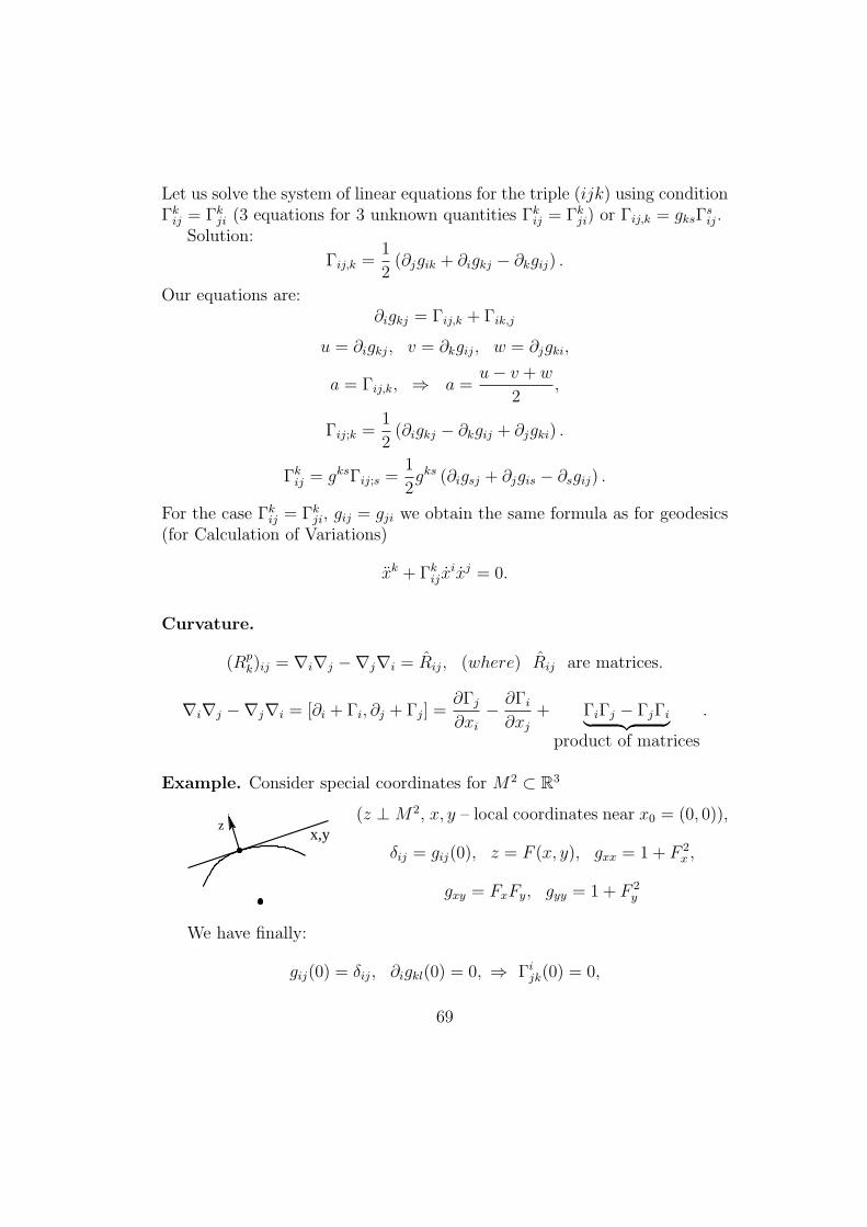
Example. Consider special coordinates for M2 ⊂ R3
zx,y
(z ⊥M2, x, y – local coordinates near x0 = (0, 0)),
δij = gij(0), z = F (x, y), gxx = 1 + F 2x ,
gxy = FxFy, gyy = 1 + F 2y
We have finally:
gij(0) = δij, ∂igkl(0) = 0, ⇒ Γijk(0) = 0,
69
∂Γkij∂xl
=? Calculation is required.
Conclusions from calculations (later):
1. Rij;kl = gisRsj;kl = Rkl;ij.
2. Rji;kl = −Rij;kl = Rij;lk.
For n = 2 we have: i, j, k, l = 1, 2. The whole curvature tensor Rij,kl canbe defined by 1 scalar function R (why?)
Rij = Rki,kj Ricci Curvature
R = Rii, Ri
j = gisRsj, Scalar Curvature
Gauss Theorem. R/2 = Gaussian Curvature of the surface M2 ⊂ R3
(Calculation later).
For n = 2 and M2 = S2,R2, H2 we have R = const.
For n = 3 we have: Ricci Curvature Rij completely determines the wholetensor Rij,kl. Why? They have the same number of components.
Curvature of Rn, Sn, Hn.
R =
0,> 0,< 0.
?
Curvature of conformally Euclidean metric gij = ϕ2(x)δij.What is “Curvature of 2-directions”?Einstein equation: n = 4, gij-indefinite.
Rij −1
2Rgij = λgij, no matter, only gravity.
“cosmological constant” λ = 0.Curvature of metrics in the compact groups like SOn, Un, . . . ?What does it mean – “Constant curvature”?
∇iRij,kl ≡ 0 “locally symmetric spaces”.
Compact groups, in particular.
70
Appendix to Lecture 15.
Γkij = gksΓij;s =1
2gks (gsj,i + ∂jgis,j − gij,s) .
Our notation:∂f/∂xk ≡ f, k
Riq =∂Γq∂xi− ∂Γi∂xq
+ ΓiΓq − ΓqΓi, where Γi = Γkij.
Our system:
gij(0) = δij, gij,p(0) = 0, gij(0) = δij = gij(0), gij,p(0) = 0
Riq = Rjk;iq = Rjk;iq, (x, y = 0, 0).
∂Γjqk∂xi
=1
2(gjk,iq + gqj,ik − gqk,ij)
∂Γjik∂xq
=1
2(gjk,iq + gij,qk − gik,qj)
2Rjk;iq = gjk,iq + gqj,ik − gqk,ij − gjk,iq − gij,qk + gik,qj =
= gqj,ik − gqk,ij − gij,qk + gik,qj
(All formulas are valid at the point 0,0)
Lecture 16. Tensor fields. Curvature as a
tensor field. Gaussian curvature for surfaces
in R3 .
• What is a tensor field?
• Calculations: Curvature is a tensor field.
• Calculation of Curvature in the special coordinates.
• Algebraic properties of Curvature Tensor.
• Gauss Theorem for M2 ⊂ R3.
71
• Curvature Tensor at the most symmetric spaces Rn, Sn, Hn.
What is a Tensor? (Scalars, vectors, covectors, inner products, Rieman-nian Curvature.)
Mn, x1, . . . , xn -local coordinates. Tensor field of the type (k, l) is definedby components:
T i1,...,ikj1,...,jl(x), dim = nk+l, Vector bundle Ψ :Mn → Tensors,
such that for x = x(y) we have change
T p1,...,pkq1,...,ql(y) = T i1,...,ikj1,...,jl
(x(y))
(∂xj1
∂yq1· . . .
)(∂yp1
∂xi1· . . .
)Examples: T i(x) – vector field.
T p(y) = T i(x(y))∂yp
∂xi,
Tq(y) = Tj(x(y))∂xj
∂yq,
Inner products:
gpq = gij∂xi
∂yp∂xj
∂yq.
Linear operators:
apq = aij∂yp
∂xi∂xj
∂yq.
Inner product of covectors:
gpq = gij∂yp
∂xi∂yq
∂xj.
Operations: linear (sum), product of tensors(1)
T IJ ·
(2)
T PQ = T IPJQ, permutation
of indexes: gij → gji.
“Trace”: T ...i......i... =∑
i T...i......i... .
Calculations.
Ψ = GΨ′, ∇i = ∂i + Γi, ∇′i = ∂i + Γ′
i, Γ′i = G−1ΓiG+G−1∂iG.
72
Rij = ∇i∇j −∇j∇i = ∂iΓj − ∂jΓi + ΓiΓj − ΓjΓi.
Theorem: R′ij = ∇′
i∇′j −∇′
j∇′i = G−1RijG.
Proof: We have ∂iG−1 = −G−1 ∂iGG−1, because ∂i(G
−1G) = 0 = ∂iG−1G+
G−1 ∂iG = 0. O.K.
∂iΓ′j = ∂i(G
−1ΓjG+G−1∂jG) = −(G−1(∂iG)G−1ΓjG)+
+G−1∂iΓjG+G−1Γj∂iG−G−1∂iG G−1∂jG+G−1∂i∂jG,
Γ′iΓ
′j = (G−1ΓiG+G−1∂iG)(G
−1ΓjG+G−1∂jG) =
= G−1ΓiΓjG+G−1(∂iG)G−1ΓjG+G−1Γi∂jG+ (G−1∂iG)(G
−1∂jG)
Conclusion: R′ij = G−1RijG.
Corollary. Rij;kl is a tensor for tangent bundle T ∗(Mn), Rkl = Rs
p;kl.
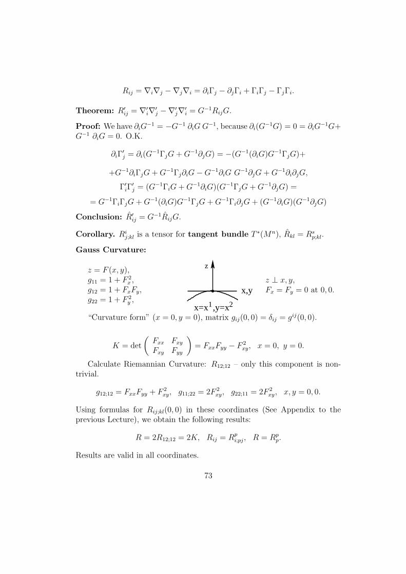
Gauss Curvature:
z = F (x, y),g11 = 1 + F 2
x ,g12 = 1 + FxFy,g22 = 1 + F 2
y ,
z
x,y
1x=x ,y=x 2
z ⊥ x, y,Fx = Fy = 0 at 0, 0.
“Curvature form” (x = 0, y = 0), matrix gij(0, 0) = δij = gij(0, 0).
K = det
(Fxx FxyFxy Fyy
)= FxxFyy − F 2
xy, x = 0, y = 0.
Calculate Riemannian Curvature: R12;12 – only this component is non-trivial.
g12;12 = FxxFyy + F 2xy, g11;22 = 2F 2
xy, g22;11 = 2F 2xy, x, y = 0, 0.
Using formulas for Rij;kl(0, 0) in these coordinates (See Appendix to theprevious Lecture), we obtain the following results:
R = 2R12;12 = 2K, Rij = Rpi;pj, R = Rp
p.
Results are valid in all coordinates.
73
Consider a pair of vector fields ξ, η. Define ∇η = ηi∇i.
Curvature:Rηξ = ∇η∇ξ −∇ξ∇η −∇[η,ξ],
[η, ξ] = [ηi∂i, ξj∂j] = (ηi ∂ξj/∂xi − ξi ∂ηj/∂xi)∂j.
We haveRη,ξ = Rijη
iξj (Matrix)
for any vector bundle.
Quadratic Form (tangent bundle, symmetric connection)
Rij;kl = Rkl;ij = −Rji;kl −Rij;lk,
< ij >= − < ji > – basic vectors in ∧2Rn.
Curvature along 2-direction: let η, ξ be unit orthogonal vectors (in the Rie-mannian Metric)
|η| = 1, |ξ| = 1, < η, ξ >= 0.
Then the sectional curvature is:
Rij;kl ηkξlηiξj︸ ︷︷ ︸
Sum by k,l
= R < η ∧ ξ, η ∧ ξ > .
Metrics: Sn, Rn, Hn.
Quadratic form Rij;kl is determined by one constant R. All curvatures ifall 2-directions are the same at all points:
• Positive for Sn.
• Negative for Hn.
• 0 for Rn.
Symmetry Groups are On+1 for Sn, Iso(Rn) and O1,n for Hn. Dimensionof these groups is n(n + 1)/1. Any points can be mapped to any point(homogeneous space). Any unit tangent vector cam be mapped to any unittangent vector.
74
Every pair (x, v) can be mapped to every pair (y, w), where x, y arepoints, v, w are tangent vectors at the points x, y respectively, |v| = |w| = 1.
Remark. GroupOn acts homogeneously on the space Vn,k of orthonormalk-frames (τ1, . . . , τk) in Rn, τi ⊥ τj, |τi| = 1.
Vn,k=“Stiefel Manifold”, Vn,1 = Sn−1, Vn,n = On.
Homework 5.
1. Prove that RP2\point is diffeomorphic to MOBIUS BAND.
2. Prove that KLEIN BOTTLE
b
b
a a is the same as
RP2#RP2 , where # is “connected sum”
3. Prove that metric of Sn, Rn, Hn can be written in the form
a) dl2 = dρ2 + sin2ρ (dΩ)2 , Sn ,
where (dΩ)2 is the metric of Sn−1 ,
b) dl2 = dr2 + r2 (dΩ)2 , Rn ,
c) dl2 = dχ2 + sh2ρ (dΩ)2 , Hn .
4. Introduce “conformal coordinates” in Sn
x0
x1 xn
0
N
...
75
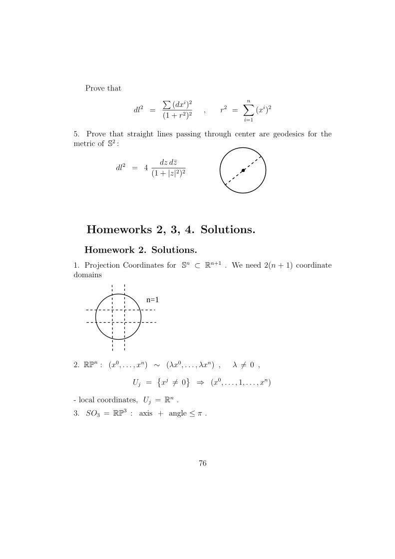
Prove that
dl2 =
∑(dxi)2
(1 + r2)2, r2 =
n∑i=1
(xi)2
5. Prove that straight lines passing through center are geodesics for themetric of S2 :
dl2 = 4dz dz
(1 + |z|2)2
Homeworks 2, 3, 4. Solutions.
Homework 2. Solutions.
1. Projection Coordinates for Sn ⊂ Rn+1 . We need 2(n + 1) coordinatedomains
n=1
2. RPn : (x0, . . . , xn) ∼ (λx0, . . . , λxn) , λ = 0 ,
Uj =xj = 0
⇒ (x0, . . . , 1, . . . , xn)
- local coordinates, Uj = Rn .
3. SO3 = RP3 : axis + angle ≤ π .
76
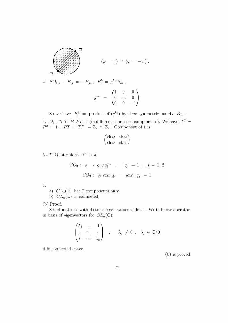
−π
π
(φ = π) ∼= (φ = −π) .
4. SO1,2 : Bij = − Bji , Bki = gks Bsi ,
gks =
1 0 00 −1 00 0 −1
So we have Bk
i = product of (gks) by skew symmetric matrix Bsi .
5. O1,1 ∋ T, P, PT, 1 (in different connected components). We have T 2 =P 2 = 1 , PT = TP − Z2 × Z2 . Component of 1 is(
chψ shψshψ chψ
)
6 - 7. Quaternions R4 ∋ q
SO3 : q → q1 q q−11 , |qj| = 1 , j = 1, 2
SO3 : q1 and q2 − any |qj| = 1
8.a) GLn(R) has 2 components only.b) GLn(C) is connected.
(b) Proof.Set of matrices with distinct eigen-values is dense. Write linear operators
in basis of eigenvectors for GLn(C):λ1 . . . 0...
. . ....
0 . . . λn
, λj = 0 , λj ∈ C\0
it is connected space.(b) is proved.
77
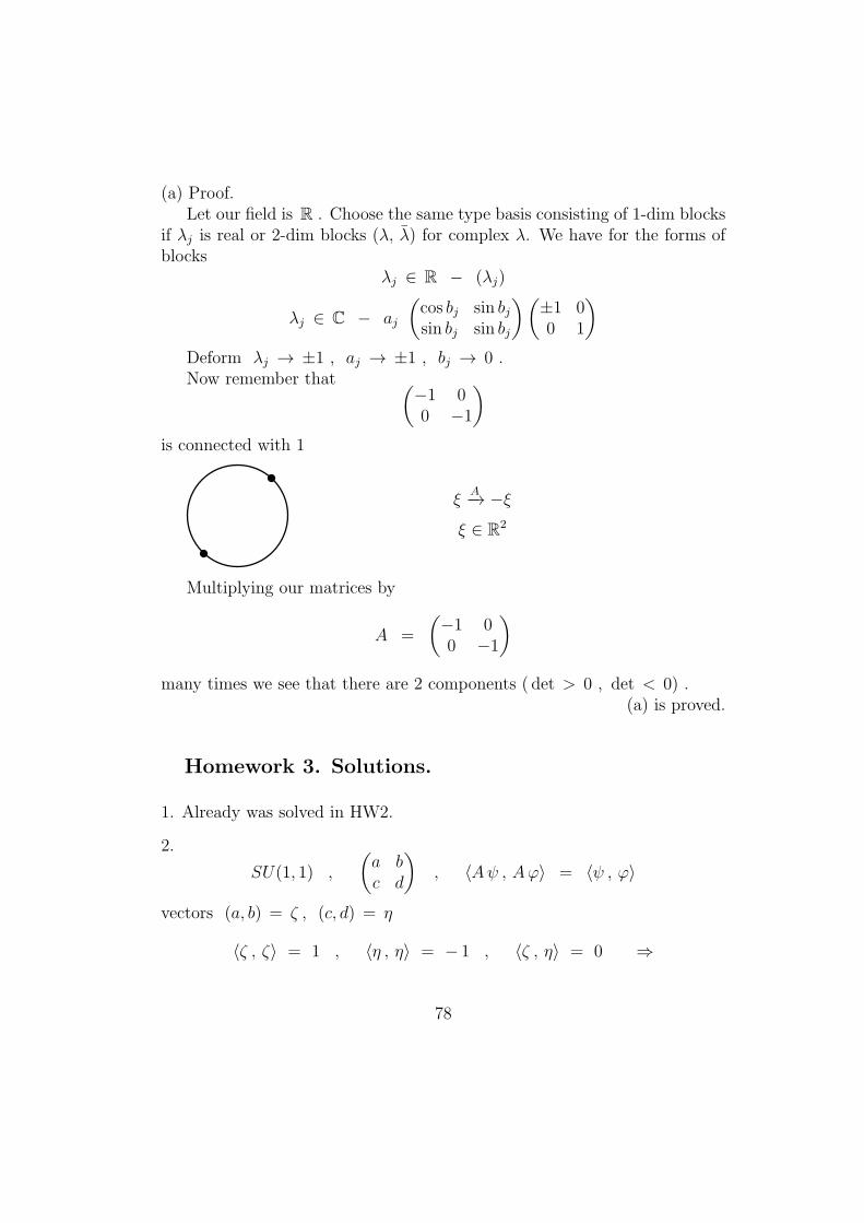
(a) Proof.Let our field is R . Choose the same type basis consisting of 1-dim blocks
if λj is real or 2-dim blocks (λ, λ) for complex λ. We have for the forms ofblocks
λj ∈ R − (λj)
λj ∈ C − aj
(cos bj sin bjsin bj sin bj
)(±1 00 1
)Deform λj → ±1 , aj → ±1 , bj → 0 .Now remember that (
−1 00 −1
)is connected with 1
ξA−→ −ξ
ξ ∈ R2
Multiplying our matrices by
A =
(−1 00 −1
)many times we see that there are 2 components ( det > 0 , det < 0) .
(a) is proved.
Homework 3. Solutions.
1. Already was solved in HW2.
2.
SU(1, 1) ,
(a bc d
), ⟨Aψ , Aφ⟩ = ⟨ψ , φ⟩
vectors (a, b) = ζ , (c, d) = η
⟨ζ , ζ⟩ = 1 , ⟨η , η⟩ = − 1 , ⟨ζ , η⟩ = 0 ⇒
78
|a|2 − |b|2 = 1 , |c|2 − |d|2 = − 1 , a c − b d = 0
solution: (a bb a
), a a − b b = 1
SL2(R) : e1 , e2 → a e1 + b e2 , c e1 + d e2
a d − b c = 1 , a, b, c, d ∈ R
Take basise = e1 + i e2 , e = e1 − i e2
e1 = (e + e)/2 , e2 = (e − e)/2i
In the new basis we have
e → 1
2
[(a+ d − i (b− c)
)e +
(a− d + i (b+ c)
)e]
= q e + p e
e → 1
2
[(a− d − i (b+ c)
)e +
(a+ d + i (b− c)
)e]
= p e + q e
where
q q − p p =1
4
((a+d)2 + (b−c)2 − (a−d)2 − (b+c)2
)= a d − b c = 1
4. SL2(R) ∼= S1 × R2 (?)
A ∈ SL2(R) ⇒ A =
(cosφ sinφ− sinφ cosφ
)×(λ µ0 1/λ
)where λ ∈ R+\0 ∼= R , µ ∈ R .
Remark. Every “semisimple” Lie Group is topologically a product:G ∼= K × RN , where K is a “compact group” and RN is a “Borelsubgroup” (upper triangle).
4.dl2 = dθ2 + sin2θ (dφ)2 , S2 ⊂ R3
For polar coordinates in R2 : x = ρ cosφ , y = ρ sinφ we have
dl2 = dρ2 + ρ2 (dφ)2
79
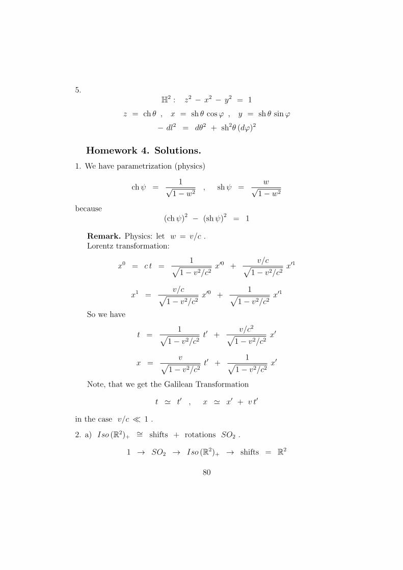
5.H2 : z2 − x2 − y2 = 1
z = ch θ , x = sh θ cosφ , y = sh θ sinφ
− dl2 = dθ2 + sh2θ (dφ)2
Homework 4. Solutions.
1. We have parametrization (physics)
chψ =1√
1− w2, shψ =
w√1− w2
because(chψ)2 − (shψ)2 = 1
Remark. Physics: let w = v/c .Lorentz transformation:
x0 = c t =1√
1− v2/c2x′0 +
v/c√1− v2/c2
x′1
x1 =v/c√
1− v2/c2x′0 +
1√1− v2/c2
x′1
So we have
t =1√
1− v2/c2t′ +
v/c2√1− v2/c2
x′
x =v√
1− v2/c2t′ +
1√1− v2/c2
x′
Note, that we get the Galilean Transformation
t ≃ t′ , x ≃ x′ + v t′
in the case v/c ≪ 1 .
2. a) Iso (R2)+ ∼= shifts + rotations SO2 .
1 → SO2 → Iso (R2)+ → shifts = R2
80
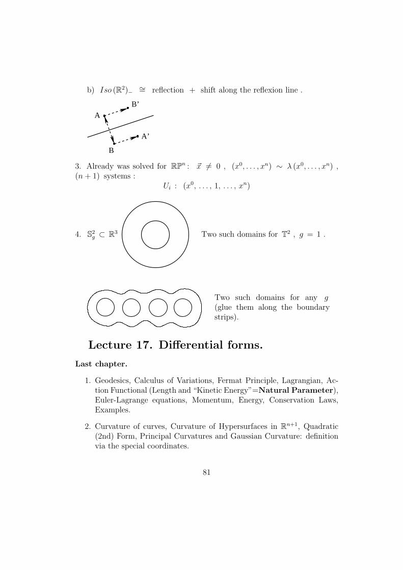
b) Iso (R2)− ∼= reflection + shift along the reflexion line .
A
B’
A’
B
3. Already was solved for RPn : x = 0 , (x0, . . . , xn) ∼ λ (x0, . . . , xn) ,(n+ 1) systems :
Ui : (x0, . . . , 1, . . . , xn)
4. S2g ⊂ R3 Two such domains for T2 , g = 1 .
Two such domains for any g(glue them along the boundarystrips).
Lecture 17. Differential forms.
Last chapter.
1. Geodesics, Calculus of Variations, Fermat Principle, Lagrangian, Ac-tion Functional (Length and “Kinetic Energy”=Natural Parameter),Euler-Lagrange equations, Momentum, Energy, Conservation Laws,Examples.
2. Curvature of curves, Curvature of Hypersurfaces in Rn+1, Quadratic(2nd) Form, Principal Curvatures and Gaussian Curvature: definitionvia the special coordinates.
81
3. Vector Bundles and Differential-Geometrical (Linear) Connection, Cur-vature, Gauge Transformation for Connection and Curvature.Parallel Transport.
4. Tangent Bundle and “Christoffel Symbols”, Cotangent Bundle, Ten-sor Bundles (Inner Products), Geodesics (new definition), compatibil-ity with Riemannian Metric. Symmetric Connections. Formulas forChristoffel Symbols and Riemannian Curvature. Special Coordinates.
5. Symmetries of the Riemannian Curvature Tensor, Ricci Tensor andScalar Curvature. Examples. Einstein Equations (n = 4). Curvaturefor n = 2. Gauss Theorem. Curvature for n = 3. Curvature of Rn, Sn,Hn.
Next chapter. Differential forms.
• m = 0: Differential 0-form is a scalar function
f(x) :Mn → R.
• m = 1: Differential 1-form is a covector field ω written in the form
ω =∑
ωi(x)dxi.
• m = n Differential n-form = object of integration:
Ω = f(x)dx1 ∧ . . . ∧ dxn, (locally)
such that for x = x(y) we have
Ω = f(x(y))dx1 ∧ . . . ∧ dxn, dxi =∂xi
∂yjdyj, (summation in j)
Definition. Differential k-from in Mn is a smooth quantity Ω which locallyin every Chart of Atlas (x1, . . . , xn) can be written in the form
Ω =∑I
fI(x) dxi1 ∧ . . . ∧ dxik︸ ︷︷ ︸
dxI
= fIdxI ,
82
where I = (i1 < i2 . . . < ik), and for x = x(y) we have
Ω = fI(x(y))dxi = gJ(y)dy
J , dyJ = dyj1 ∧ . . . ∧ dyjk , j1 < j2 < . . . < jk.
The symbols dxi form an Associative Algebra under multiplication ∧(exterior product), such that
dxi ∧ dxj = −dxj ∧ dxi,
(bilinear, associative.)
Examples:
1.
(∑i
aidxi)∧ (
∑j
bjdxj) =
∑ij
aibjdxi∧dxj =
∑i<j
(aibj−ajbi)dxi∧dxj.
2. Change of coordinates:
x = x(y), dxi =∂xi
∂yjdyj, (summation in j)
3. Corollary:
(a) k ≤ n.
(b) Ωn = f(x)dx1 ∧ . . . ∧ dxn.
Lemma. C∞ differential forms is a ring ∧∗(Mn,R) such that every C∞-mapf :Mn → Nm there is a natural “induced map” of rings:
f ∗ : ∧∗(Nm)→ ∧∗(Mn),
commuting with all algebraic operations (addition, multiplication ∧).
Proof. “Change of coordinates”
x = x(y), yf→ x, ⇒
[dxi
f∗⇒ ∂xi
∂yjdyj (sum)
]commutes with change of coordinates in N and M and with all algebraicoperations like ∧.
83
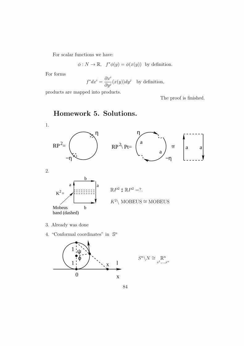
For scalar functions we have:
ϕ : N → R, f ∗ϕ(y) = ϕ(x(y)) by definition.
For forms
f ∗dxi =∂xi
∂yj(x(y))dyj by definition,
products are mapped into products.The proof is finished.
Homework 5. Solutions.
1.
η
−η
RP =2RP \ Pt=2
η
−η
=a
aa a
2.
K =2
a a
b
b
Mobeusband (dashed)
RP 2 ♯ RP 2 =?.
K2\ MOBEUS ∼= MOBEUS
3. Already was done
4. “Conformal coordinates” in Sn
0 x
l
ψϕ
x1
1
Sn\N ∼= Rn
x1,...,xn
84
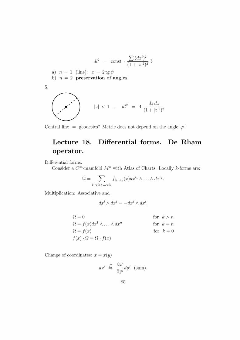
dl2 = const ·∑
(dxi)2
(1 + |x|2)2?
a) n = 1 (line): x = 2 tgψb) n = 2 preservation of angles
5.
|z| < 1 , dl2 = 4dz dz
(1 + |z|2)2
Central line = geodesics? Metric does not depend on the angle φ !
Lecture 18. Differential forms. De Rham
operator.
Differential forms.Consider a C∞-manifold Mn with Atlas of Charts. Locally k-forms are:
Ω =∑
i1<i2<...<ik
fi1...ik(x)dxi1 ∧ . . . ∧ dxik .
Multiplication: Associative and
dxi ∧ dxj = −dxj ∧ dxi.
Ω = 0 for k > n
Ω = f(x)dx1 ∧ . . . ∧ dxn for k = n
Ω = f(x) for k = 0
f(x) · Ω = Ω · f(x)
Change of coordinates: x = x(y)
dxif∗⇒ ∂xi
∂yjdyj (sum).
85
Functorial properties: g :My→ N
x, x = x(y).
G∗Ω =∑
fI(x(y))dxi1 ∧ . . . ∧ dxik , dxi ⇒ ∂xi
∂yj(x(y))dyj.
Algebra of forms.
∧∗(M) =n∑k=0
∧k(M),
g∗(Ω1 ∧ Ω2) = g∗Ω1 ∧ g∗Ω2.
Integration of forms.
1. ∫±P
f(x) = ±f(P ), k = 0, ±P = “point with orientation”.
2. ∫D
f(x)dx1 ∧ . . . ∧ dxn = ordinary integral
D-domain (local). To integrate over large domains, one can write∫D
Ω =∑q
ϕq(x)Ω,
where ∑q
ϕq(x) ≡ 1, ϕq is a C∞ function,
ϕq ≡ 0 outside of small domain Dnq ⊂ Mn. The family ϕq is called
“Partition of Unity”.
3. Let Ω be a k-form and g : Dk →Mn, g is C∞. By definition:∫g(Dk)
Ω =
∫Dk
g∗Ω − integral of k-form in k-ball Dk.
86
Properties: Integration of forms does not depend on local coordinates bothinMn and Dk (restrict the k-form to the k-dimensional body and integrate).
Differentiation of forms:
d : ∧k(Mn)→ ∧k+1(Mn)
1. df is usual differential.
2. d(dxi1 ∧ . . . ∧ dxik) = 0.
3. d(fdxi1 ∧ . . . ∧ dxik) = df ∧ dxi1 ∧ . . . ∧ dxik .
Example:
d(fidxi) = dfi ∧ dxi =
∑i,j
∂fi∂xj
dxj ∧ dxi =∑i<j
(∂fj∂xi− ∂fi∂xj
)dxi ∧ dxj.
Examples of forms:Momentum (pi) in Calculus of Variations. Differential of function
df =∑ ∂f
∂xidxi.
Electric field (Ei)-covector field.2-forms: Magnetic field in R3. B = Bαβdx
αdxβ.Electromagnetic field in R4 = (x0, x1, x2, x3).
F = Fijdxi ∧ dxj = cFojdt ∧ dxα +Bαβdx
α ∧ dxβ,
i, j = 0, 1, 2, 3, α, β = 1, 2, 3, x0 = cdt, F0α = Eα – electric field, Bαβ = Fαβ– magnetic field.
Symplectic 2-form in the cotangent space T∗Mn with local coordinates
(xi, pi)
Ω =n∑i=1
dxi ∧ dpi
Ω ∧ . . . ∧ Ω︸ ︷︷ ︸n times
− volume forms in T∗(Mn).
It defines nondegenerate inner product given by matrix
gij =
(0 1n−1n 0
)skew symmetric.
87
Kahler Riemannian Metric in Complex Space (Manifolds) with complexlinear coordinates (z1, . . . , zn).
dl2 =∑α,β
gα,βdzαdzβ > 0.
Coordinates: (z1, . . . , zn, z1, . . . , zn). Associated 2-form is
Ω =i
2
∑α,β
gα,βdzα ∧ dzβ, z = x+ iy.
Examples: n=1.
dl2 = gαβdzαdzβ =
dzdz : R2
dzdz
(1± |z|2)2:
S2
H2
Ω =i
2
dz ∧ dz(1± |z|2)2
=dx ∧ dy
(1± (x2 + y2))2− Area Form.
Theorem: The operator d is well-defined in ∧k(Mn) by the definition above.It commutes with C∞-maps g :M → N and has the following properties:
1. d(Ωk ∧ Ωl) = (dΩk) ∧ Ωl + (−1)kΩk ∧ (dΩl).
2. d d = 0.
Proof:
a)
d(g∗f(x(y))
)= g∗df : d(g∗f) = d(f(x(y))) =
∂f
∂xi∂xi
∂yjdyj = g∗df.
b)d(dxi) = d(0) ∧ dxi = 0,
d(g∗dxi) = d
(dxi
dyjdyj)
=∂2xi
∂yj∂yqdyq ∧ dyj ≡ 0.
88
So d commutes with the map g∗ for k = 1.For k > 1 our result is obvious by the following reason: d(dxi1 ∧ . . . ∧
dxik) = 0. Let us prove now that the Statement 1 of the Theorem. LetΩk = f · dxi1 ∧ . . . ∧ dxik , Ωl = g · dxj1 ∧ . . . ∧ dxjl .
d(Ωk ∧ Ωl) = d[(f · dxi1 ∧ . . . ∧ dxik) ∧ (g · dxj1 ∧ . . . ∧ dxjl)
]=
= (df · g + f · dg) ∧ dxi1 ∧ . . . ∧ dxik ∧ dxj1 ∧ . . . ∧ dxjl =
= df ∧ dxi1 ∧ . . . ∧ dxik ∧ gdxj1 ∧ . . . ∧ dxjl+
+(−1)kfdxi1 ∧ . . . ∧ dxik ∧ dg ∧ dxj1 ∧ . . . ∧ dxjl =
= (dΩk) ∧ Ωl + (−1)kΩk ∧ (dΩl).
Let us prove now that d d = 0.
d(f · dxi1 ∧ . . . ∧ dxik) = df ∧ dxi1 ∧ . . . ∧ dxik =∂f
∂xjdxj ∧ dxi1 ∧ . . . ∧ dxik .
dd(f ·dxi1∧. . .∧dxik) = d(df)∧dxi1∧. . .∧dxik−df∧d(dxi1∧. . .∧dxik) ≡ 0.
Theorem is proved.We have:
d (Ajdxj)︸ ︷︷ ︸
“covector field”
=∑i<j
(∂Aj∂xi− ∂Ai∂xj
)dxi ∧ dxj.︸ ︷︷ ︸
“curl”=2-form
Let n = 3, B12 → B3, B13 → −B2, B23 → B1.
d(B12dx1∧dx2+B13dx
1∧dx3+B23dx2∧dx3) =
(∂B1
∂x1+∂B2
∂x2+∂B3
∂x3
)︸ ︷︷ ︸
divB
dx1∧dx2∧dx3
Faraday Laws:
n = 3 :
n = 4 :
a) dB = 0, Magnetic fieldb) dE = 1
c∂B∂t, E = Eαdx
α,d(Fijdx
i ∧ dxj) = 0. Electromagnetic field
89
Lecture 19. Differential forms. Cohomol-
ogy.
Consider the algebra of differential forms on a manifold Nm. Let Ω ∈∧k(Nm). Then dΩ ∈ ∧k+1(Nm). Consider a map f : M → N . Let uscheck, that f ∗dΩ = df ∗Ω.
Proof. Let ϕ : N → R, f ∗ϕ(y) = ϕ(x(y)).
f ∗dϕ(y) = f ∗(∂ϕ
∂xidxi)
=∂ϕ
∂xi(x(y))f ∗(dxi) =
∂ϕ
∂xi(x(y))
∂xi
∂yjdyj =
∂(f ∗ϕ)
∂yjdyj. O.K. f ∗d = df ∗,
for scalars and dxi. But the product ∧ commutes with f ∗. Every form is acombination of ϕ(x) · dxi1 ∧ . . . ∧ dxik . So we have
f ∗d = df∗ for all k ≥ 0.
Homology (Cohomology).
Hk(Mn,R) = Ker d/ Im d in ∧k (Mn).
Ker d ⊂ ∧k : Ω | dΩ = 0 closed forms
Im d ⊂ ∧k : Ω | Ω = dΩ′ exact forms
Examples: a) k = 0 ⇒ Ω = ϕ is locally constant.Conclusion: H0(Mn,R) = Rp, where p is the number of components.
Closed Forms.
1. Forms with constant coefficients in Rn or in T n = Rn/Zn: Ω =∑aIdx
I ,aI = const.
2. Closed 1-form
ω =∑
ψi(x)dxi, dω =
∑i<j
(∂ψj∂xi− ∂ψi∂xj
)dxi ∧ dxj.
90
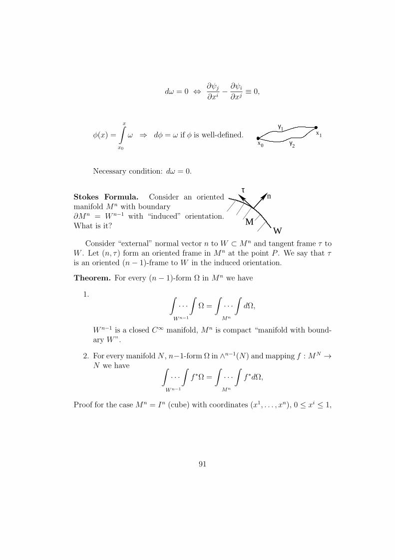
dω = 0 ⇔ ∂ψj∂xi− ∂ψi∂xj≡ 0,
ϕ(x) =
x∫x0
ω ⇒ dϕ = ω if ϕ is well-defined.x0
x1
γ
γ
1
2
Necessary condition: dω = 0.
Stokes Formula. Consider an orientedmanifold Mn with boundary∂Mn = W n−1 with “induced” orientation.What is it? M
W
τn
Consider “external” normal vector n to W ⊂Mn and tangent frame τ toW . Let (n, τ) form an oriented frame in Mn at the point P . We say that τis an oriented (n− 1)-frame to W in the induced orientation.
Theorem. For every (n− 1)-form Ω in Mn we have
1. ∫· · ·∫
Wn−1
Ω =
∫· · ·∫
Mn
dΩ,
W n−1 is a closed C∞ manifold, Mn is compact “manifold with bound-ary W”.
2. For every manifoldN , n−1-form Ω in ∧n−1(N) and mapping f :MN →N we have ∫
· · ·∫
Wn−1
f ∗Ω =
∫· · ·∫
Mn
f ∗dΩ,
Proof for the case Mn = In (cube) with coordinates (x1, . . . , xn), 0 ≤ xi ≤ 1,
91
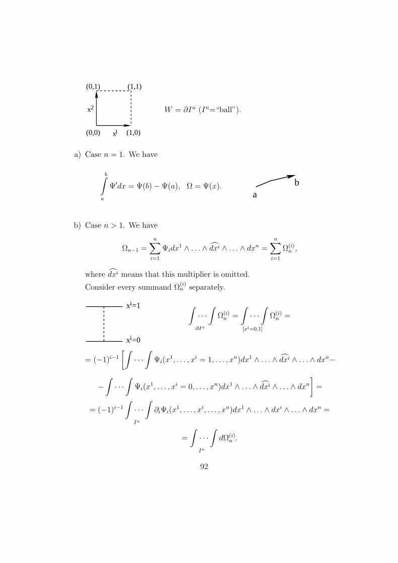
(0,0) (1,0)
(0,1) (1,1)
1x
2x W = ∂In (In=“ball”).
a) Case n = 1. We have
b∫a
Ψ′dx = Ψ(b)−Ψ(a), Ω = Ψ(x).a
b
b) Case n > 1. We have
Ωn−1 =n∑i=1
Ψidx1 ∧ . . . ∧ dxi ∧ . . . ∧ dxn =
n∑i=1
Ω(i)n ,
where dxi means that this multiplier is omitted.
Consider every summand Ω(i)n separately.
x =1i
x =0i
∫· · ·∫
∂In
Ω(i)n =
∫· · ·∫
[xi=0,1]
Ω(i)n =
= (−1)i−1
[∫· · ·∫
Ψi(x1, . . . , xi = 1, . . . , xn)dx1 ∧ . . . ∧ dxi ∧ . . . ∧ dxn−
−∫· · ·∫
Ψi(x1, . . . , xi = 0, . . . , xn)dx1 ∧ . . . ∧ dxi ∧ . . . ∧ dxn
]=
= (−1)i−1
∫· · ·∫
In
∂iΨi(x1, . . . , xi, . . . , xn)dx1 ∧ . . . ∧ dxi ∧ . . . ∧ dxn =
=
∫· · ·∫
In
dΩ(i)n .
92
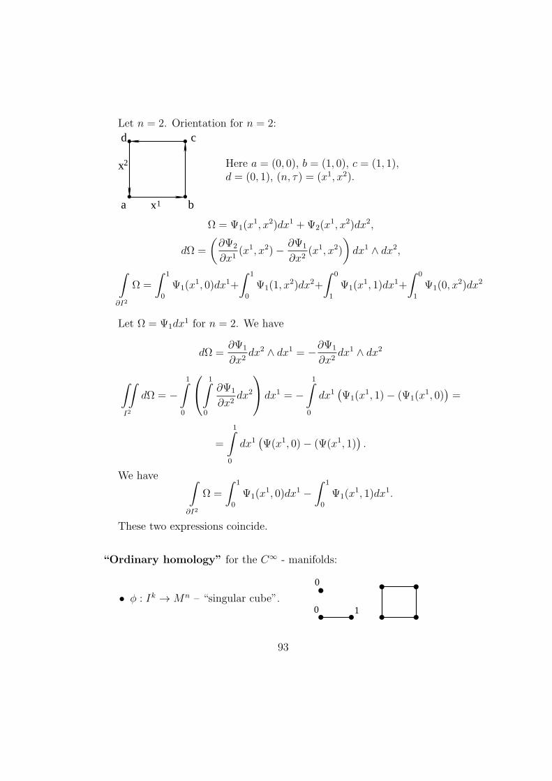
Let n = 2. Orientation for n = 2:
x
c
ba
d
x
2
1
Here a = (0, 0), b = (1, 0), c = (1, 1),d = (0, 1), (n, τ) = (x1, x2).
Ω = Ψ1(x1, x2)dx1 +Ψ2(x
1, x2)dx2,
dΩ =
(∂Ψ2
∂x1(x1, x2)− ∂Ψ1
∂x2(x1, x2)
)dx1 ∧ dx2,∫
∂I2
Ω =
∫ 1
0
Ψ1(x1, 0)dx1+
∫ 1
0
Ψ1(1, x2)dx2+
∫ 0
1
Ψ1(x1, 1)dx1+
∫ 0
1
Ψ1(0, x2)dx2
Let Ω = Ψ1dx1 for n = 2. We have
dΩ =∂Ψ1
∂x2dx2 ∧ dx1 = −∂Ψ1
∂x2dx1 ∧ dx2
∫∫I2
dΩ = −1∫
0
1∫0
∂Ψ1
∂x2dx2
dx1 = −1∫
0
dx1(Ψ1(x
1, 1)− (Ψ1(x1, 0)
)=
=
1∫0
dx1(Ψ(x1, 0)− (Ψ(x1, 1)
).
We have ∫∂I2
Ω =
∫ 1
0
Ψ1(x1, 0)dx1 −
∫ 1
0
Ψ1(x1, 1)dx1.
These two expressions coincide.
“Ordinary homology” for the C∞ - manifolds:
• ϕ : Ik →Mn – “singular cube”.10
0
93
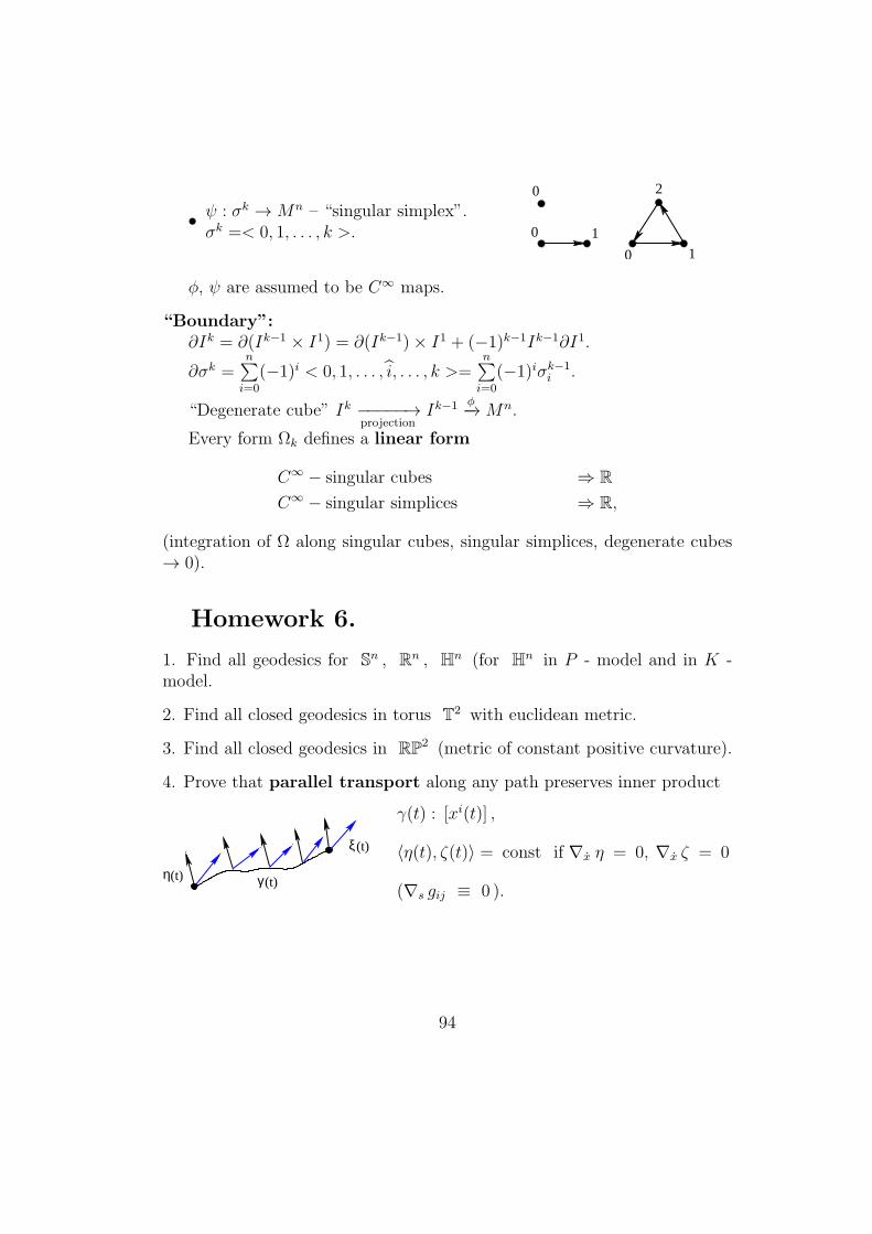
• ψ : σk →Mn – “singular simplex”.σk =< 0, 1, . . . , k >. 10
0
0 1
2
ϕ, ψ are assumed to be C∞ maps.
“Boundary”:∂Ik = ∂(Ik−1 × I1) = ∂(Ik−1)× I1 + (−1)k−1Ik−1∂I1.
∂σk =n∑i=0
(−1)i < 0, 1, . . . , i, . . . , k >=n∑i=0
(−1)iσk−1i .
“Degenerate cube” Ik −−−−−→projection
Ik−1 ϕ−→Mn.
Every form Ωk defines a linear form
C∞ − singular cubes ⇒ RC∞ − singular simplices ⇒ R,
(integration of Ω along singular cubes, singular simplices, degenerate cubes→ 0).
Homework 6.
1. Find all geodesics for Sn , Rn , Hn (for Hn in P - model and in K -model.
2. Find all closed geodesics in torus T2 with euclidean metric.
3. Find all closed geodesics in RP2 (metric of constant positive curvature).
4. Prove that parallel transport along any path preserves inner product
γ(t)η(t)
ξ (t)
γ(t) : [xi(t)] ,
⟨η(t), ζ(t)⟩ = const if ∇x η = 0, ∇x ζ = 0
(∇s gij ≡ 0 ).
94
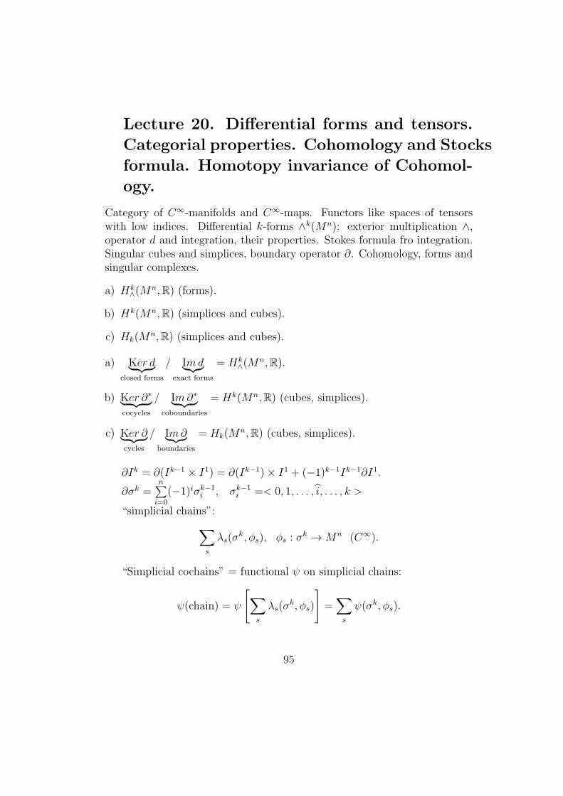
Lecture 20. Differential forms and tensors.
Categorial properties. Cohomology and Stocks
formula. Homotopy invariance of Cohomol-
ogy.
Category of C∞-manifolds and C∞-maps. Functors like spaces of tensorswith low indices. Differential k-forms ∧k(Mn): exterior multiplication ∧,operator d and integration, their properties. Stokes formula fro integration.Singular cubes and simplices, boundary operator ∂. Cohomology, forms andsingular complexes.
a) Hk∧(M
n,R) (forms).
b) Hk(Mn,R) (simplices and cubes).
c) Hk(Mn,R) (simplices and cubes).
a) Ker d︸ ︷︷ ︸closed forms
/ Imd︸︷︷︸exact forms
= Hk∧(M
n,R).
b) Ker ∂∗︸ ︷︷ ︸cocycles
/ Im∂∗︸ ︷︷ ︸coboundaries
= Hk(Mn,R) (cubes, simplices).
c) Ker ∂︸ ︷︷ ︸cycles
/ Im∂︸︷︷︸boundaries
= Hk(Mn,R) (cubes, simplices).
∂Ik = ∂(Ik−1 × I1) = ∂(Ik−1)× I1 + (−1)k−1Ik−1∂I1.
∂σk =n∑i=0
(−1)iσk−1i , σk−1
i =< 0, 1, . . . , i, . . . , k >
“simplicial chains”:∑s
λs(σk, ϕs), ϕs : σ
k →Mn (C∞).
“Simplicial cochains” = functional ψ on simplicial chains:
ψ(chain) = ψ
[∑s
λs(σk, ϕs)
]=∑s
ψ(σk, ϕs).
95
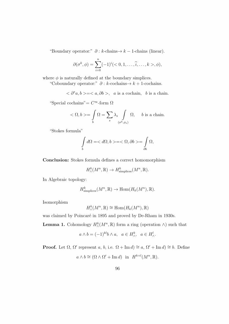
“Boundary operator:” ∂ : k-chains→ k − 1-chains (linear).
∂(σk, ϕ) =n∑i=0
(−1)i(< 0, 1, . . . , i, . . . , k >, ϕ),
where ϕ is naturally defined at the boundary simplices.“Coboundary operator:” ∂ : k-cochains→ k + 1-cochains.
< ∂∗a, b >=< a, ∂b >, a is a cochain, b is a chain.
“Special cochains”= C∞-form Ω
< Ω, b >=
∫b
Ω =∑s
λs
∫(σk,ϕs)
Ω, b is a chain.
“Stokes formula”∫b
dΩ =< dΩ, b >=< Ω, ∂b >=
∫∂b
Ω,
Conclusion: Stokes formula defines a correct homomorphism
Hk∧(M
n,R)→ Hksimplices(M
n,R).
In Algebraic topology:
Hksimplices(M
n,R)→ Hom(Hk(Mn),R).
IsomorphismHk
∧(Mn,R) ∼= Hom(Hk(M
n),R)
was claimed by Poincare in 1895 and proved by De-Rham in 1930s.
Lemma 1. Cohomology Hk∧(M
n,R) form a ring (operation ∧) such that
a ∧ b = (−1)klb ∧ a, a ∈ Hk∧, a ∈ H l
∧.
Proof. Let Ω, Ω′ represent a, b, i.e. Ω + Im d) ∼= a, Ω′ + Im d) ∼= b. Define
a ∧ b ∼= (Ω ∧ Ω′ + Im d) in Hk+l(Mn,R).
96
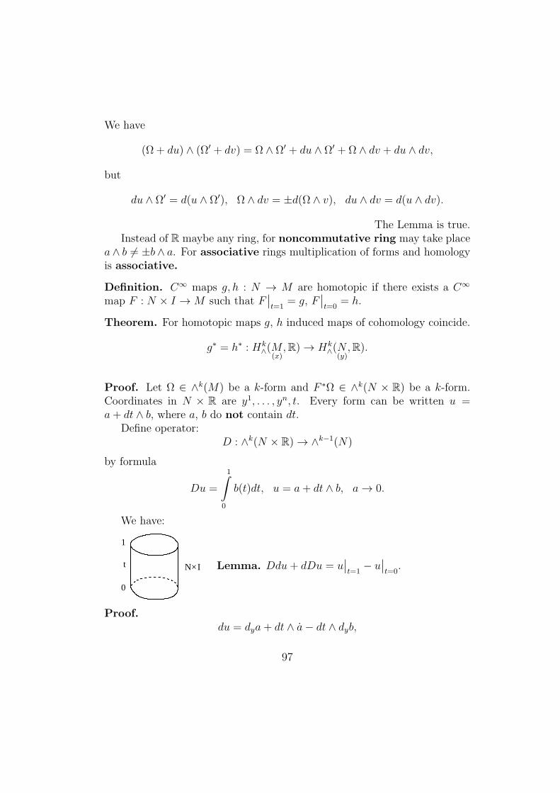
We have
(Ω + du) ∧ (Ω′ + dv) = Ω ∧ Ω′ + du ∧ Ω′ + Ω ∧ dv + du ∧ dv,
but
du ∧ Ω′ = d(u ∧ Ω′), Ω ∧ dv = ±d(Ω ∧ v), du ∧ dv = d(u ∧ dv).
The Lemma is true.Instead of R maybe any ring, for noncommutative ring may take place
a∧ b = ±b∧ a. For associative rings multiplication of forms and homologyis associative.
Definition. C∞ maps g, h : N → M are homotopic if there exists a C∞
map F : N × I →M such that F∣∣t=1
= g, F∣∣t=0
= h.
Theorem. For homotopic maps g, h induced maps of cohomology coincide.
g∗ = h∗ : Hk∧(M
(x),R)→ Hk
∧(N(y),R).
Proof. Let Ω ∈ ∧k(M) be a k-form and F ∗Ω ∈ ∧k(N × R) be a k-form.Coordinates in N × R are y1, . . . , yn, t. Every form can be written u =a+ dt ∧ b, where a, b do not contain dt.
Define operator:D : ∧k(N × R)→ ∧k−1(N)
by formula
Du =
1∫0
b(t)dt, u = a+ dt ∧ b, a→ 0.
We have:
N I
0
1
t Lemma. Ddu+ dDu = u∣∣t=1− u∣∣t=0.
Proof.du = dya+ dt ∧ a− dt ∧ dyb,
97
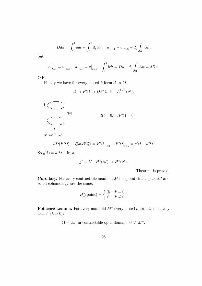
Ddu =
∫ 1
0
adt−∫ 1
0
dybdt = a∣∣t=1− a∣∣t=0− dy
∫ 1
0
bdt,
but
a∣∣t=1
= u∣∣t=1, a
∣∣t=0
= u∣∣t=0,
∫ 1
0
bdt = Du, dy
∫ 1
0
bdt = dDu.
O.K.Finally we have for every closed k-form Ω in M :
Ω→ F ∗Ω→ DF ∗Ω in ∧k−1 (N).
N I
0
1
t
y
dΩ = 0, dF ∗Ω = 0,
so we have
dD(F ∗Ω) +XXXXXDd(F ∗Ω) = F ∗Ω∣∣t=1− F ∗Ω
∣∣t=0
= g∗Ω− h∗Ω.
So g∗Ω = h∗Ω + Im d,
g∗ ≡ h∗ : Hk(M)→ Hk(N).
Theorem is proved.
Corollary. For every contractible manifoldM like point, Ball, space Rn andso on cohomology are the same:
H∗∧(point) =
R, k = 0,0, k = 0.
Poincare Lemma. For every manifoldMn every closed k-form Ω is “locallyexact” (k > 0):
Ω = dω in contractible open domain U ⊂Mn.
98
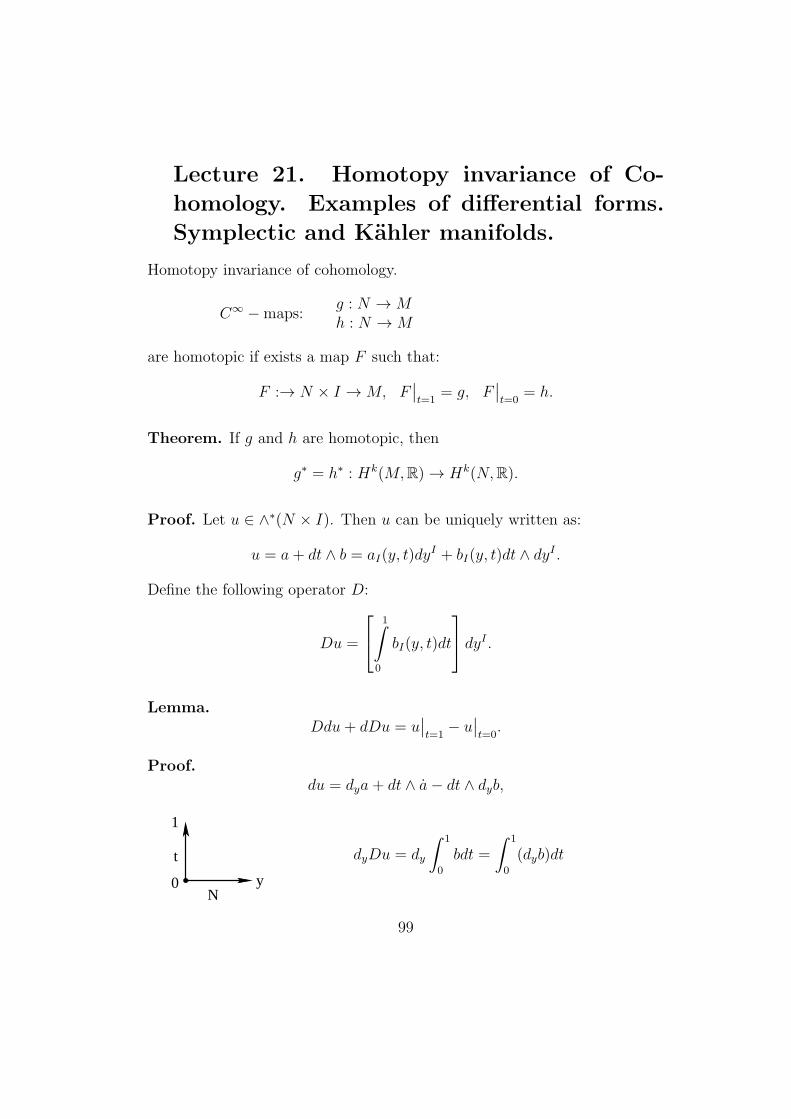
Lecture 21. Homotopy invariance of Co-
homology. Examples of differential forms.
Symplectic and Kahler manifolds.
Homotopy invariance of cohomology.
C∞ −maps:g : N →Mh : N →M
are homotopic if exists a map F such that:
F :→ N × I →M, F∣∣t=1
= g, F∣∣t=0
= h.
Theorem. If g and h are homotopic, then
g∗ = h∗ : Hk(M,R)→ Hk(N,R).
Proof. Let u ∈ ∧∗(N × I). Then u can be uniquely written as:
u = a+ dt ∧ b = aI(y, t)dyI + bI(y, t)dt ∧ dyI .
Define the following operator D:
Du =
1∫0
bI(y, t)dt
dyI .Lemma.
Ddu+ dDu = u∣∣t=1− u∣∣t=0.
Proof.du = dya+ dt ∧ a− dt ∧ dyb,
t
0
1
yN
dyDu = dy
∫ 1
0
bdt =
∫ 1
0
(dyb)dt
99
Ddu = D(d(a+ dt ∧ b)) = D(dya+ dt ∧ a− dt ∧ dyb) =
= a∣∣t=1− a∣∣t=0− dy
∫ 1
0
bdt = a∣∣t=1− a∣∣t=0− dDu.
O.K.
Proof of the Theorem.
F :→ N × I →MΩ,
F ∗dΩ = df ∗Ω = 0,
dD(F ∗Ω) +XXXXXDd(F ∗Ω) = F ∗Ω∣∣t=1− F ∗Ω
∣∣t=0
= h∗Ω− g∗Ω.
g∗ ≡ h∗ : Hk(M)→ Hk(N).
O.K.
Homotopy equivalent manifolds N , M :
∃ N −→ϕM −→
ψN
such that
ψ · ϕ is homotopic to 1N : N → N
ϕ · ψ is homotopic to 1M : M →M.
Corollary: M and N are homotopy equivalent implies:
ϕ∗ : H∗(M)→ H∗(N)
ψ∗ : H∗(N)→ H∗(M).
are isomorphisms of rings.In particular, H∗(Rn) = H∗(Dn) = H∗(M) = H∗(point), where M is
any contractible manifold (map 1 : M → M is homotopic to const:M → point).
Poincare Lemma. Every closed k-form Ω is “locally exact” (k > 0).
Examples of forms
100
1. k = 0, df = 0 ⇒ f = const (in every component).
H0(M) = Rp, where p = number of components.
2. Mn is an oriented manifold. Every n-form Ω is closed: dΩ = 0 (obvi-ous). Riemannian metric in Mn generates a “volume form”
Ω = dnσ =√det gijdx
1 ∧ . . . ∧ dxn locally in oriented atlas.
Form Ω = dnσ is closed and not exact for closed (compact) manifoldsbecause ∫
Mn
Ω = volumeM > 0.
So Hn(Mn) = 0 for closed oriented manifolds. For connected nonori-ented manifolds and and manifolds with boundary we have Hn(Mn) =0 (not proved yet).
3. “Nondegenerate 2-forms”:
Ω =∑i<j
Ωijdxi ∧ dxj (locally)
detΩij = 0, Ωij = −Ωji we have n = 2k.
Theorem. For every 2-form in 2k-dimensional manifold we have:
1
k!Ω ∧ . . . ∧ Ω︸ ︷︷ ︸
k times
=√
detΩijdx1 ∧ . . . ∧ dx2k.
Proof. Let Mk = Rn and Ωij = const.
Step 1. Choose such basis that
Ωij =
(0 1
−1 0
), Ω =
k∑i=1
dxi ∧ dpi.
Step 2. Proof Theorem in this basis:(k∑i=1
dxi ∧ dpi
)k
= k! dx1 ∧ dp1 ∧ . . . ∧ dxk ∧ dpk.
101
We have:
(dxi ∧ dpi) ∧ (dxj ∧ dpj) = (dxj ∧ dpj) ∧ (dxi ∧ dpi).
Step 3. Return to the original basis. Both sides are n-forms andtransform in the same way.
So Theorem is proved.
Lemma. Every skew-symmetric inner product can be reduced to theform
Ωij =
0 1 0−1 0 00 0 0
,
Proof (for nondegenerate forms). For every vector e there exists e′
such that < e, e′ >= 1. Find orthogonal compliment to the subspace(e, e′). Iterate this process. Our Lemma follows.
Remark.√detΩij is a polynomial of the matrix entries if Ωij = −Ωji.
It is called “Pfaffian”.
Definition. Manifold M2k is called “simplistic” if there exists a 2-formΩijdx
i ∧ dxj such that detΩij = 0 and dΩ = 0.
Examples.
a) T∗(Mk). We have
Ω =k∑i=1
dxi ∧ dpi.
b) Kahler (complex manifolds). Complex coordinates (z1, . . . , zn) (locally).
o < gαβdzαdzβ − Riemannian Metric.
Ω =i
2
∑α,β
gαβdzα ∧ dzβ, dΩ = 0, det gαβ = 0.
Corollary. Every simplectic manifold is oriented.
Proof. Ωk =√detΩijdx
1 ∧ . . . ∧ dx2k is a “volume form”.
102
Lecture 22. Symplectic Manifolds and Hamil-
tonian Systems. Poisson brackets. Preser-
vation of Symplectic form by Hamiltonian
System.
Symplectic form. Mn, Ω, dΩ = 0, n = 2k, Ωk = k!dnσ – volume.Property (without proof): locally there exists a system of coordinates
x1, . . . , xk, p1, . . . , pk such that
Ω =k∑i=1
dxi ∧ dpi.
Example. Consider cotangent bundle of a C∞ manifold Mn = T∗Nk, with
coordinates (x, p). Change of coordinates
x = x(y), pj = pi∂xi
∂yj
Lemma 1. 2-form Ω is well-defined (independent of the choice of coordinatesin N).
Proof. Ω =∑i
dxi ∧ dpi, Ω =k∑i=1
dyi ∧ dpi. Why Ω = Ω.
dpj = dpi∂xi
∂yj+ pi
∂2xi
∂yj∂ykdyk
∑j
dyj ∧ dpj =∑ij
dyj ∧ dpi∂xi
∂yj+
XXXXXXXXXXXdpi
∂2xi
∂yj∂ykdyj ∧ dyk =
=∑ij
∂xi
∂yjdyj ∧ dpi =
∑i
dxi ∧ dpi.
O.K.More generic simplectic form in T∗N is∑
dxi ∧ dpi +e
cB = ΩB, B =
∑i<j
bij(x)dxi ∧ dxj, dB = 0.
103
For k = 3 it is “Magnetic Field” (correction of simplectic form).Hamiltonian system in: T∗N =M is defined by “Hamiltonian” H(x, p),
xi =∂H
∂pi
pi = −∂H
∂xi
Another form: Take covector field (dH). Take inner product given bysimplistic form Ω =
∑dxi ∧ dpi.
Ωij =
(0 1
−1 0
).
Construct vector field ηH = Ω−1(dH).
Dynamical System.z = η(z), z = (x, p),
x = Hp, p = −Hx.
“Poisson Bracket”.
f, g =< df, dg >Ω= − < dg, df >Ω .
It provides the structure of Lie algebra.For any functions f(x, p) we have:
f = H, f.
We have H,H = 0 – conservation of energy.
Geodesics. M = T∗N , H = 12gijpipj. Lagrangian L = 1
2gijx
ixj,
H = xi∂L
∂xi− L, pi =
∂L
∂xi.
Euler-Lagrange equations:
pi =∂L
∂xi⇔ xi + Γijkx
jxk = 0.
104
Theorem 1. In every compact closed simplectic manifold Mn (n = 2k)with form Ω (nondegenerate, we have
H2j(M) = 0, j = 1, . . . , k.
Proof. We know that Ωk = k! volume, so∫Ωk = 0. Therefore H2j = 0,
because Ω2j can not be exact (if Ω2j is exact then Ω2k is exact.)
Theorem 2. For any simplectic manifold Mn and Hamiltonian system withHamiltonian H : Mn → R simplectic form is preserved by mapping St :Mn →Mn (time shift by our system).
Proof. Locally we choose such coordinates (x1, . . . , xk, p1, . . . , pk) that Ω =k∑i=1
dxi ∧ dpi (Darboux).
Our system is:
pi = −∂H
∂xi, xi =
∂H
∂pi
Small time shift is:
St : pi → pi + pit+O(t2)
xi → xi + xit+O(t2)
S∗t pi = pi + pit+O(t2)
S∗t x
i = xi + xit+O(t2)
We have
S∗t (dx
i∧dpi) =∑i
(dxi+xit)∧(dpi+pit) =∑i
[dxi + td
∂H
∂pi
]∧[dpi − td
∂H
∂xi
]=
=∑i
dxi ∧ dpi + t
[d∂H
∂pi∧ dpi − dxi ∧ d
∂H
∂xi
]=
= Ω+∑ij
t
[∂2H
∂pi∂pjdpj ∧ dpi +
∂2H
∂pi∂xjdxj ∧ dpi −
dxi ∧ ∂2H
∂xi∂xjdxj − dxi ∧ ∂2H
∂xi∂pkdpk =
]= Ω
105
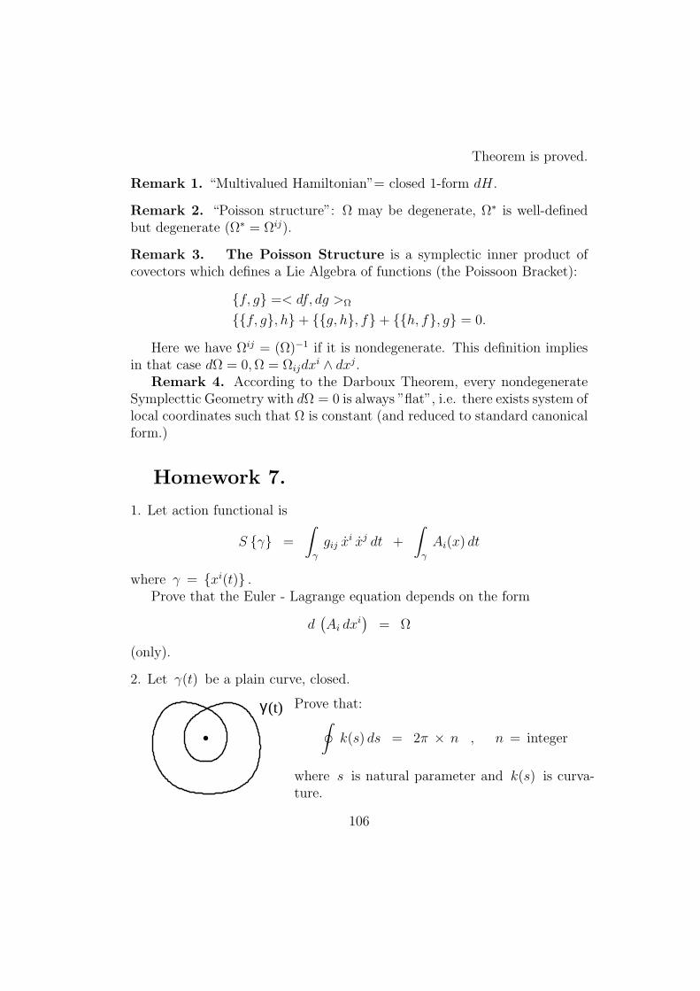
Theorem is proved.
Remark 1. “Multivalued Hamiltonian”= closed 1-form dH.
Remark 2. “Poisson structure”: Ω may be degenerate, Ω∗ is well-definedbut degenerate (Ω∗ = Ωij).
Remark 3. The Poisson Structure is a symplectic inner product ofcovectors which defines a Lie Algebra of functions (the Poissoon Bracket):
f, g =< df, dg >Ω
f, g, h+ g, h, f+ h, f, g = 0.
Here we have Ωij = (Ω)−1 if it is nondegenerate. This definition impliesin that case dΩ = 0,Ω = Ωijdx
i ∧ dxj.Remark 4. According to the Darboux Theorem, every nondegenerate
Symplecttic Geometry with dΩ = 0 is always ”flat”, i.e. there exists system oflocal coordinates such that Ω is constant (and reduced to standard canonicalform.)
Homework 7.
1. Let action functional is
S γ =
∫γ
gij xi xj dt +
∫γ
Ai(x) dt
where γ = xi(t) .Prove that the Euler - Lagrange equation depends on the form
d(Ai dx
i)
= Ω
(only).
2. Let γ(t) be a plain curve, closed.
γ(t) Prove that:∮k(s) ds = 2π × n , n = integer
where s is natural parameter and k(s) is curva-ture.
106
3. Calculate area form in R2 , S2 , H2 in the spherical (pseudospherical)coordinates (polar for R2 ).
4. Prove that
dφ = c · xdy − ydxx2 + y2
in the plane R2 .
5. Let a complex line bundle C1x be given over Mn , (x1, . . . , xn) with
an imaginary Differential - Geometric Connection AUj dxj = iAUjReal dxj ,
U ⊂ Mn , AUjReal ∈ R . Let the bundle is “unitary” (i.e. in the domains
U ∩ V change of basis eU(x) = gUV (x) eV (x) , gUV ∈ U1 = S1 (eiψ)) .Prove that 2-form
H =(HU)
=(dAUReal
)=(dAVReal
)in U ∩ V is well defined as a closed 2-form in Λ2(Mn) .
dH = 0
(first Chern class). Its integrals along the closed 2-submanifolds are always2πn, n ∈ Z.
Remark. This fact (well-known in Topology of characteristic classes)was also discovered by Dirac in 1930-50s in process of Heisenberg-Schrodingerquantization of ”Magnetic Monopole”: the Hilbert space of state is in factspace of sections of complex line bundle where vector-potential of magneticfield is a covariant derivative of sections. (The Feinman quantization throughthe path integral leads to different topology: the Action functional for mag-netic monopole is in fact a closed 1-form on the space of paths whose periodsalong 1-cycles in this space should be quantized, i.e. they should be equal to2πn, n ∈ Z assuming that the Plank constant is equal to one in our units.)
Lecture 23. Volume element in Compact Lie
groups. Averaging of differential forms and
Riemannian Metric. Cohomology of Homo-
geneous Spaces.
Homogeneous spaces. Mn = G/H, G – Lie group (compact).
107
Theorem. Let group G be compact. There exists Riemannian Metric inM = G/H s.t. g∗gij(x) = gij(x), g ∈ G, g : M → M , g(x)- action of thegroup G.
Remark. We assume that there exists a G-invariant volume form Ω inthe group G. We call it dσ(g).
Proof of the Theorem. Take any Riemannian Metric gij(x) in M . Con-sider family of metrics g∗gij(x) = ghij(x) in M , depending on g ∈ G asparameter. Integrate: ∫
G
ggij(x)dσ(g) = Gij(x).
1. This is a Riemannian (positive!) metric.
2. This metric is G-invariant because for ψ ∈ G we have
ψ∗Gij =
∫G
ψ∗ggij(x)dσ(g) =
∫G
gψgij (x)dσ(g) =
∫G
gψgij (x)dσ(ψg)
The last identity is based on the following:
Lemma 1. In every compact Lie Group there exists a double-invariantvolume form.
Proof. Consider left-invariant metric in G : gij and its volume form Ω :h∗gij = gij, h
∗Ω = Ω. But this n-form is also right-invariant because forg → hgh−1 this form maps into itself (space of right-invariant n-forms is1-dimensional and group is compact).
So the Theorem is proved.
Theorem 2. For homogeneous manifolds with compact group G: M =G/H every closed differential form is homologous to an invariant closed form.
Proof. Let dω = 0 in ∧k(M). Consider the integral
ω =1
|G|
∫G
h∗ω dσ(h),
|G| =∫G
dσ(h), h ∈ G, h :M →M.
108
1. This is an invariant form.
2. This is a closed form:
dω =1
|G|
∫G
h∗ω dσ(h) =1
|G|
∫G
h∗(dω) dσ(h) = 0.
3. This from represents the same cohomology class as ω: all forms h∗ωbelongs to the same cohomology class if the group is connected. Soall “integral sums” belong to the same cohomology class.
So our Theorem follows.
Examples.
1. Spheres Sn, G = SOn+1. Only invariant forms are k = 0 (scalars ) andk = n. So we have:
H0(Sn) = Hn(Sn) = R.
2. Tori T n = Rn/Zn, G = T n (abelian group). Spaces of invariant formsare ∧kRn. All of them are closed: dω = 0 for invariant forms, soH∗(T n) = ∧(v1, . . . , vn).
3. Sn1 × . . . × Snk . Forms v1, . . . , vk, dim vk = k. We have v2j = 0 onlyrelations.
H∗(Sn1 × . . .× Snk) = v1, . . . , vk, v2j = 0.
4. Cohomology of RP 2n+1 are the same as for S2n+1 ( H∗( ,R) ).
Cohomology of RP 2n are 0 (k > 0).
Cohomology of CP n are generated by 2-form Ω and its powers:
1,Ω,Ω2, . . . ,Ωn.
Action of SOn and Un in Rn and Cn. Invariant differential forms:
109
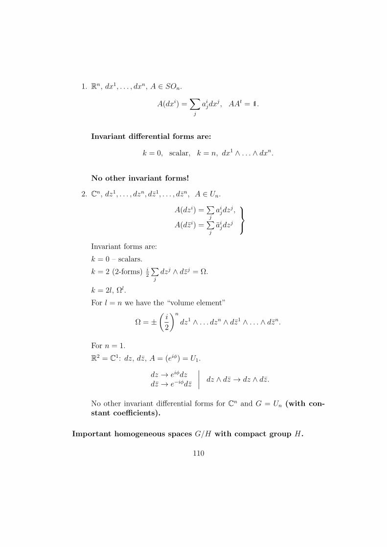
1. Rn, dx1, . . . , dxn, A ∈ SOn.
A(dxi) =∑j
aijdxj, AAt = 1.
Invariant differential forms are:
k = 0, scalar, k = n, dx1 ∧ . . . ∧ dxn.
No other invariant forms!
2. Cn, dz1, . . . , dzn, dz1, . . . , dzn, A ∈ Un.
A(dzi) =∑j
aijdzj,
A(dzi) =∑j
aijdzj
Invariant forms are:
k = 0 – scalars.
k = 2 (2-forms) i2
∑j
dzj ∧ dzj = Ω.
k = 2l, Ωl.
For l = n we have the “volume element”
Ω = ±(i
2
)ndz1 ∧ . . . dzn ∧ dz1 ∧ . . . ∧ dzn.
For n = 1.
R2 = C1: dz, dz, A = (eiϕ) = U1.
dz → eiϕdzdz → e−iϕdz
∣∣∣∣ dz ∧ dz → dz ∧ dz.
No other invariant differential forms for Cn and G = Un (with con-stant coefficients).
Important homogeneous spaces G/H with compact group H.
110
1. Sn = SOn+1/SOn.
S2n−1 = Un/Un−1.
S4n−1 = Spn/Spn−1.
2. CP n = Un+1/U1 × Un = SUn+1/Un.
3. Stiefel Manifolds.
Vn,k = SOn/SOn−k (orthogonal k-frames in Rn).
V Cn,k = Un/Un−k (complex version).
4. Grassmann Manifolds.
Gn,k = SOn/SOk × SOn−k.
GCn,k = Un/Uk × Un−k
5. Lie Groups (compact, simple) G
G = G×G/G, g → h1gh−12 , h1 ∈ G, h2 ∈ G.
6. “Principal” homogeneous spaces
G = G/(1), H = 1.
Lecture 24. Volume element in Compact Lie
groups. Averaging of differential forms and
Riemannian Metric. Cohomology of Homo-
geneous Spaces.
Theorem. Let G be a compact Lie group with invariant volume elementdσ(h):
For h1, h2 : G→ G, ϕ : h→ h1hh−12 we have
ϕ∗dσ(h) = dσ(h).Let G act (from the left) in the manifold M h :M →M , h ∈ G. Group
G is connected. Then
1. Every closed differential form is homologous to an invariant form.
111
2. Operator of “Averaging” maps Hk(M) as a unit homomorphism:
ω =1
|G|
∫G
h∗ω dσ(h), h ∈ G,
0 = dω ⇒ dω = 0, ω − ω = dv, ω = dv ⇒ ω = dv,
i.e.
H∗(M) ∼= H∗inv(M) ← calculated with G− invariant forms only.
Proof was given at the previous lecture.
Examples.
1. Sn, G = SOn+1, H = SOn. Invariant forms k = 0, n only. H0 = R,Hn = R.
2. G = S3 = SU2, H = (1). Invariant forms k = 0, 1, 2, 3
∧0 = R, ∧1 = R3, ∧2 = R3, ∧0 = R,
d : ∧1 → ∧2 is an isomorphism.
3. Un+1/U1 × Un = CP n = SUn+1/Un. G = SUn+1, H = Un. H acts onCn (tangent to 1). Constant forms in Cn (all closed).
Basis: dzi1 ∧ . . . ∧ dzik ∧ dzj1 ∧ . . . ∧ dzjl , type (k, l).
Action: a ∈ Un,A(dzi) =
∑j
aijdzj,
A(dzi) =∑j
aijdzj
For n = 1.
dz → eiϕdzdz → e−iϕdz
∣∣∣∣ ⇒ invariant form dz ∧ dz.
k ≥ 1: invariant form aren∑i=1
dzi ∧ dzi and all Ωk,k = 1, . . . , n.
No other invariant forms (!).
112
Cohomology rings.
1. Tori T n = S1 × . . .× S1 = Rn/Zn
H∗(T n) = ∧(v1, . . . , vn), dimVj = 1.
2. Spheres Sn, G = SOn+1. Only invariant forms are k = 0 (scalars ) andk = n. So we have:
H0(Sn) = Hn(Sn) = R.
3. Sn1 × . . .× Snk , G = SOn1+1 × . . .× SOnk+1.
H∗(Sn) = 1, vn|v2n = 0.
H∗(Sn1× . . .×Snk) = ∧∗(1, vn1 , . . . , vnk|v2j = 0), no other relations.
4. CP n.
H∗(CP n) = 1, u, u2, . . . , un, dimu = 2, un+1 = 0, G = SUn+1, H = Un.
5. Homology of Vn,k, Gn,k can be computed using forms
H∗( ,R) =?
Vn,k = SOn/SOn−k; Gn,k = SOn/SOk × SOn−k,
V Cn,k = Un/Un−k; GC
n,k = Un/Uk × Un−k.
6. Lie Groups G (compact): G = G×G/G.
Lecture 25. Approximation and Transver-
sality.
Differential topology. C∞-manifolds, Atlases, Charts, Orientations, Ck-maps, rank of map, C∞-submanifolds: (existence),Mn ⊂ RN (Mn compact).
113
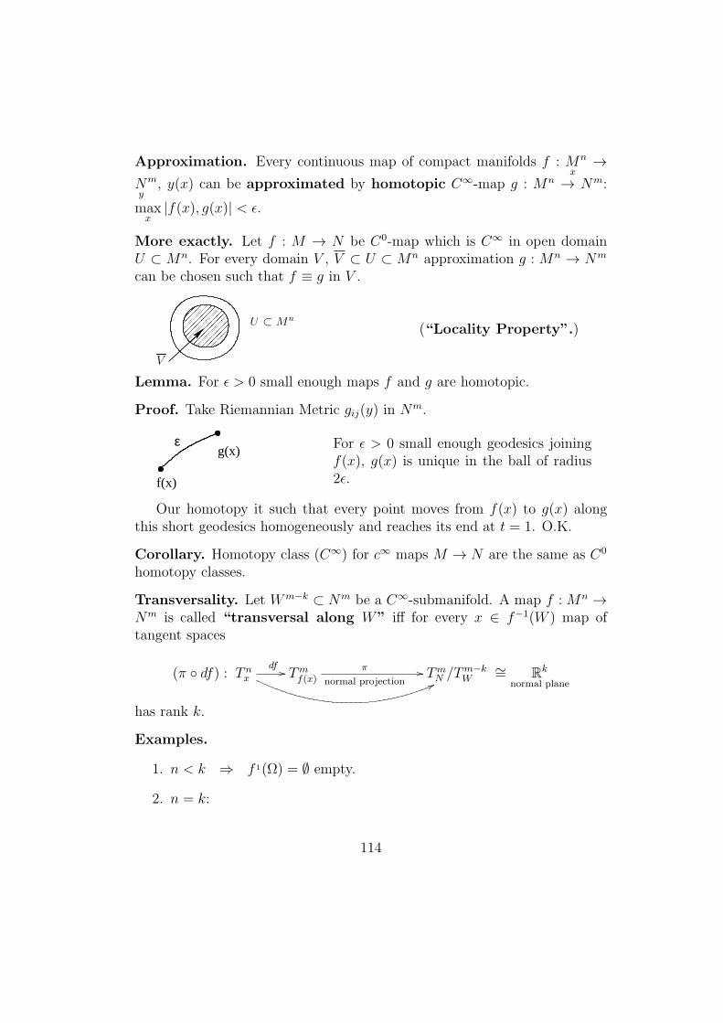
Approximation. Every continuous map of compact manifolds f : Mx
n →Ny
m, y(x) can be approximated by homotopic C∞-map g : Mn → Nm:
maxx|f(x), g(x)| < ϵ.
More exactly. Let f : M → N be C0-map which is C∞ in open domainU ⊂ Mn. For every domain V , V ⊂ U ⊂ Mn approximation g : Mn → Nm
can be chosen such that f ≡ g in V .
U ⊂ Mn
V
(“Locality Property”.)
Lemma. For ϵ > 0 small enough maps f and g are homotopic.
Proof. Take Riemannian Metric gij(y) in Nm.
ε
f(x)
g(x) For ϵ > 0 small enough geodesics joiningf(x), g(x) is unique in the ball of radius2ϵ.
Our homotopy it such that every point moves from f(x) to g(x) alongthis short geodesics homogeneously and reaches its end at t = 1. O.K.
Corollary. Homotopy class (C∞) for c∞ maps M → N are the same as C0
homotopy classes.
Transversality. Let Wm−k ⊂ Nm be a C∞-submanifold. A map f :Mn →Nm is called “transversal along W” iff for every x ∈ f−1(W ) map oftangent spaces
(π df) : T nxdf //
66Tmf(x)
π
normal projection// TmN /T
m−kW
∼= Rk
normal plane
has rank k.
Examples.
1. n < k ⇒ f 1(Ω) = ∅ empty.
2. n = k:
114
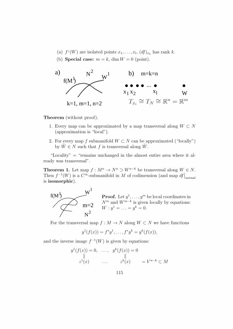
(a) f 1(W ) are isolated points x1, . . . , xl, (df)xk has rank k.
(b) Special case: m = k, dimW = 0 (point).
Txi
∼= TN
∼= R
n= R
m
1x 2x lx
f(M )11
WN2a) b) m=k=n
...
W
k=1, m=1, n=2
Theorem (without proof).
1. Every map can be approximated by a map transversal along W ⊂ N(approximation is “local”).
2. For every map f submanifold W ⊂ N can be approximated (“locally”)by W ∈ N such that f is transversal along W .
“Locality” = “remains unchanged in the almost entire area where it al-ready was transversal”.
Theorem 1. Let map f : Mn → Nn ⊃ W n−k be transversal along W ∈ N .Then f−1(W ) is a C∞-submanifold in M of codimension (and map df
∣∣normal
is isomorphic).
f(M )11
W
N2
m=2
Proof. Let y1, . . . , ym be local coordinates inNm and Wm−k is given locally by equations:W : y1 = . . . = yk = 0.
For the transversal map f :M → N along W ⊂ N we have functions
y1(f(x)) = f ∗y1, . . . , f ∗yk = yk(f(x)),
and the inverse image f−1(W ) is given by equations:
y1(f(x)) = 0, . . . , yk(f(x)) = 0∥ ∥
z1(x) . . . zk(x) = V n−k ⊂M
115
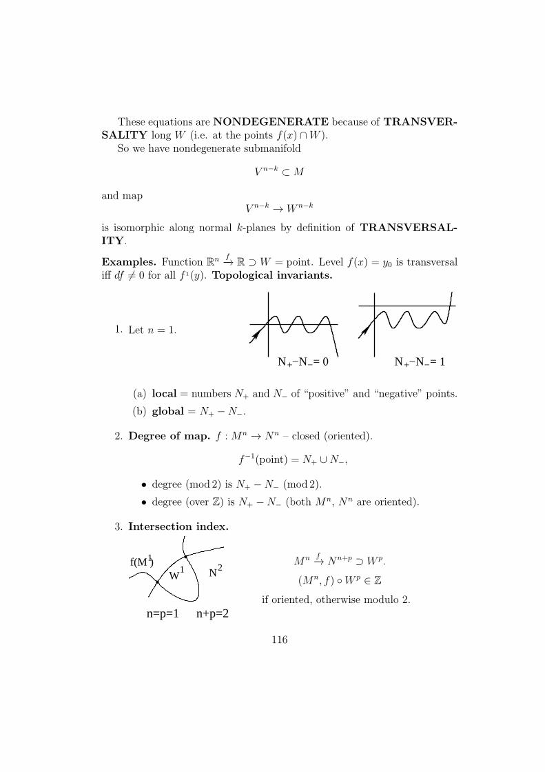
These equations are NONDEGENERATE because of TRANSVER-SALITY long W (i.e. at the points f(x) ∩W ).
So we have nondegenerate submanifold
V n−k ⊂M
and mapV n−k → W n−k
is isomorphic along normal k-planes by definition of TRANSVERSAL-ITY.
Examples. Function Rn f−→ R ⊃ W = point. Level f(x) = y0 is transversaliff df = 0 for all f 1(y). Topological invariants.
1. Let n = 1.
N −N = 1+ −N −N = 0+ −
(a) local = numbers N+ and N− of “positive” and “negative” points.
(b) global = N+ −N−.
2. Degree of map. f :Mn → Nn – closed (oriented).
f−1(point) = N+ ∪N−,
• degree (mod 2) is N+ −N− (mod 2).
• degree (over Z) is N+ −N− (both Mn, Nn are oriented).
3. Intersection index.
N21W
f(M )1
n=p=1 n+p=2
Mn f−→ Nn+p ⊃ W p.
(Mn, f) W p ∈ Z
if oriented, otherwise modulo 2.
116
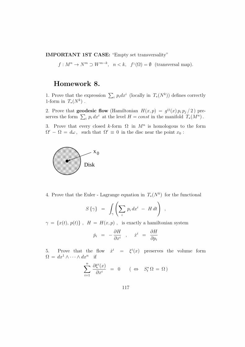
IMPORTANT 1ST CASE: “Empty set transversality”
f :Mn → Nm ⊃ Wm−k, n < k, f 1(Ω) = ∅ (transversal map).
Homework 8.
1. Prove that the expression∑
i pidxi (locally in T∗(N
k)) defines correctly1-form in T∗(N
k) .
2. Prove that geodesic flow (Hamiltonian H(x, p) = gij(x) pi pj / 2 ) pre-serves the form
∑i pi dx
i at the level H = const in the manifold T∗(Mn) .
3. Prove that every closed k-form Ω in Mn is homologous to the formΩ′ − Ω = dω , such that Ω′ ≡ 0 in the disc near the point x0 :
0x
Disk
4. Prove that the Euler - Lagrange equation in T∗(Nk) for the functional
S γ =
∫γ
(∑i
pi dxi − H dt
),
γ = x(t), p(t) , H = H(x, p) , is exactly a hamiltonian system
pi = − ∂H∂xi
, xi =∂H
∂pi
5. Prove that the flow xi = ξi(x) preserves the volume formΩ = dx1 ∧ · · · ∧ dxn if
n∑i=1
∂ξi(x)
∂xi= 0 ( ⇔ S∗
t Ω = Ω )
117
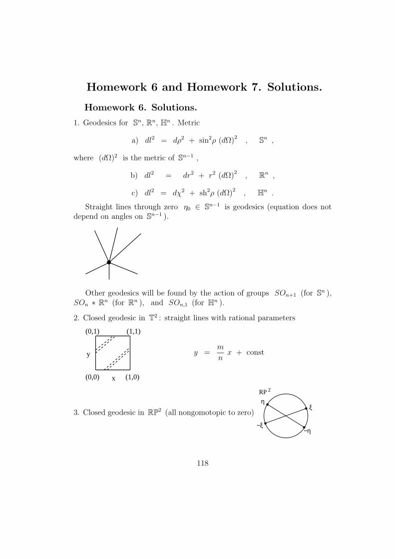
Homework 6 and Homework 7. Solutions.
Homework 6. Solutions.
1. Geodesics for Sn, Rn, Hn . Metric
a) dl2 = dρ2 + sin2ρ (dΩ)2 , Sn ,
where (dΩ)2 is the metric of Sn−1 ,
b) dl2 = dr2 + r2 (dΩ)2 , Rn ,
c) dl2 = dχ2 + sh2ρ (dΩ)2 , Hn .
Straight lines through zero η0 ∈ Sn−1 is geodesics (equation does notdepend on angles on Sn−1 ).
Other geodesics will be found by the action of groups SOn+1 (for Sn ),SOn ∗ Rn (for Rn ), and SOn,1 (for Hn ).
2. Closed geodesic in T2 : straight lines with rational parameters
(0,0) (1,0)
(0,1) (1,1)
x
y y =m
nx + const
3. Closed geodesic in RP2 (all nongomotopic to zero)
RP 2
ξη
−η−ξ
118
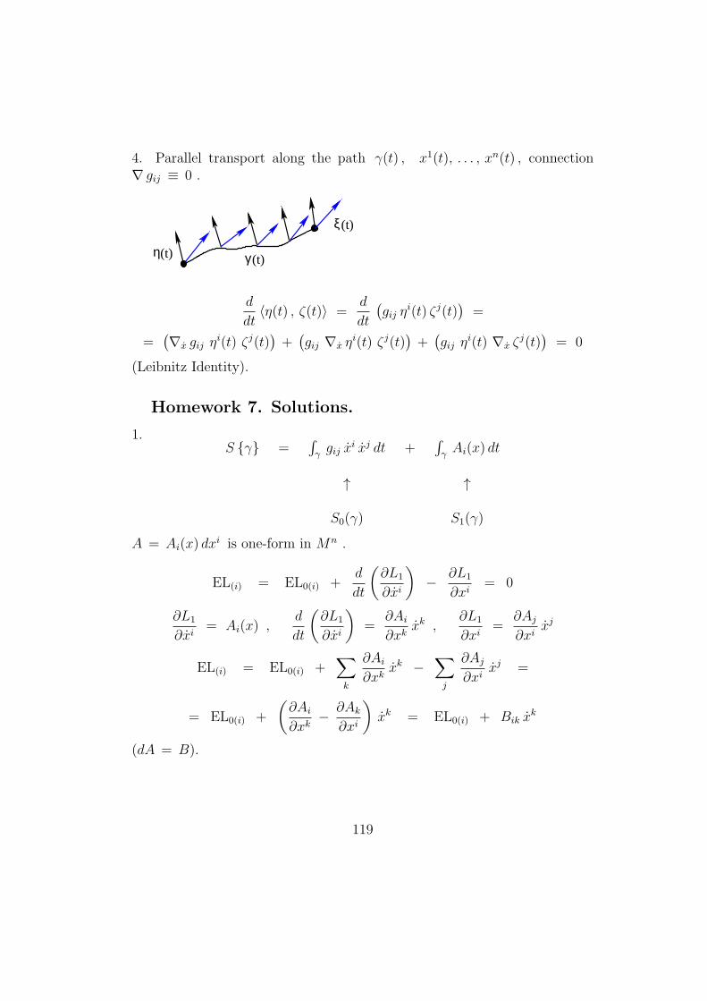
4. Parallel transport along the path γ(t) , x1(t), . . . , xn(t) , connection∇ gij ≡ 0 .
γ(t)η(t)
ξ (t)
d
dt⟨η(t) , ζ(t)⟩ =
d
dt
(gij η
i(t) ζj(t))
=
=(∇x gij η
i(t) ζj(t))+(gij ∇x η
i(t) ζj(t))+(gij η
i(t) ∇x ζj(t))
= 0
(Leibnitz Identity).
Homework 7. Solutions.
1.S γ =
∫γgij x
i xj dt +∫γAi(x) dt
↑ ↑
S0(γ) S1(γ)
A = Ai(x) dxi is one-form in Mn .
EL(i) = EL0(i) +d
dt
(∂L1
∂xi
)− ∂L1
∂xi= 0
∂L1
∂xi= Ai(x) ,
d
dt
(∂L1
∂xi
)=
∂Ai∂xk
xk ,∂L1
∂xi=
∂Aj∂xi
xj
EL(i) = EL0(i) +∑k
∂Ai∂xk
xk −∑j
∂Aj∂xi
xj =
= EL0(i) +
(∂Ai∂xk
− ∂Ak∂xi
)xk = EL0(i) + Bik x
k
(dA = B).
119
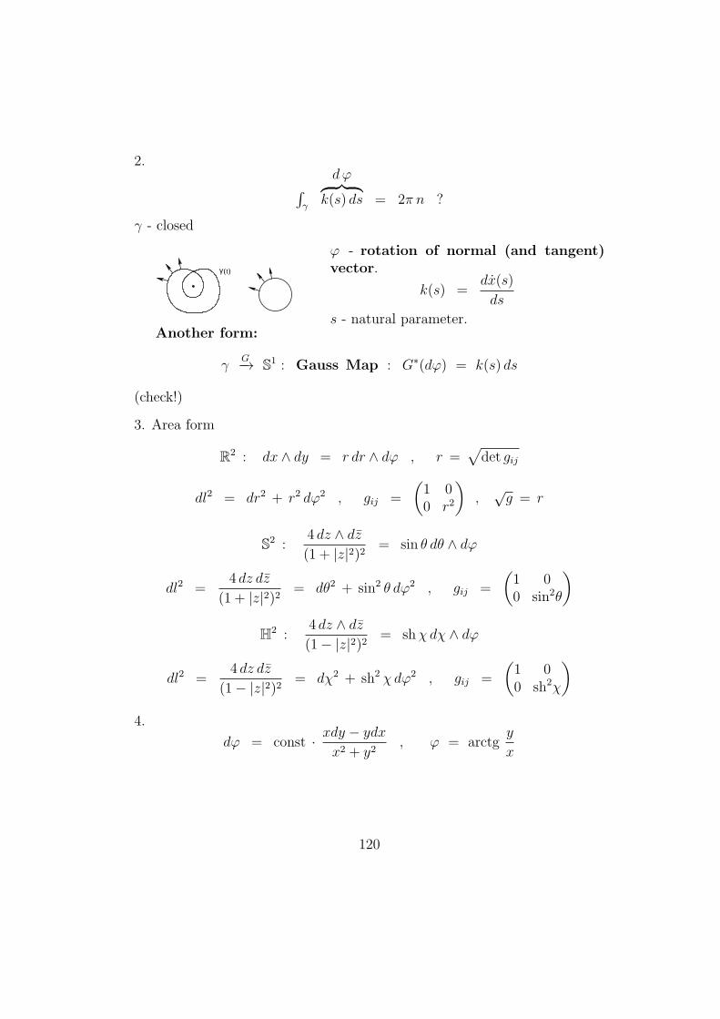
2.dφ∫
γ
︷ ︸︸ ︷k(s) ds = 2π n ?
γ - closed
γ(t)
φ - rotation of normal (and tangent)vector.
k(s) =dx(s)
ds
s - natural parameter.Another form:
γG−→ S1 : Gauss Map : G∗(dφ) = k(s) ds
(check!)
3. Area form
R2 : dx ∧ dy = r dr ∧ dφ , r =√det gij
dl2 = dr2 + r2 dφ2 , gij =
(1 00 r2
),√g = r
S2 :4 dz ∧ dz(1 + |z|2)2
= sin θ dθ ∧ dφ
dl2 =4 dz dz
(1 + |z|2)2= dθ2 + sin2 θ dφ2 , gij =
(1 00 sin2θ
)H2 :
4 dz ∧ dz(1− |z|2)2
= shχdχ ∧ dφ
dl2 =4 dz dz
(1− |z|2)2= dχ2 + sh2 χdφ2 , gij =
(1 00 sh2χ
)4.
dφ = const · xdy − ydxx2 + y2
, φ = arctgy
x
120
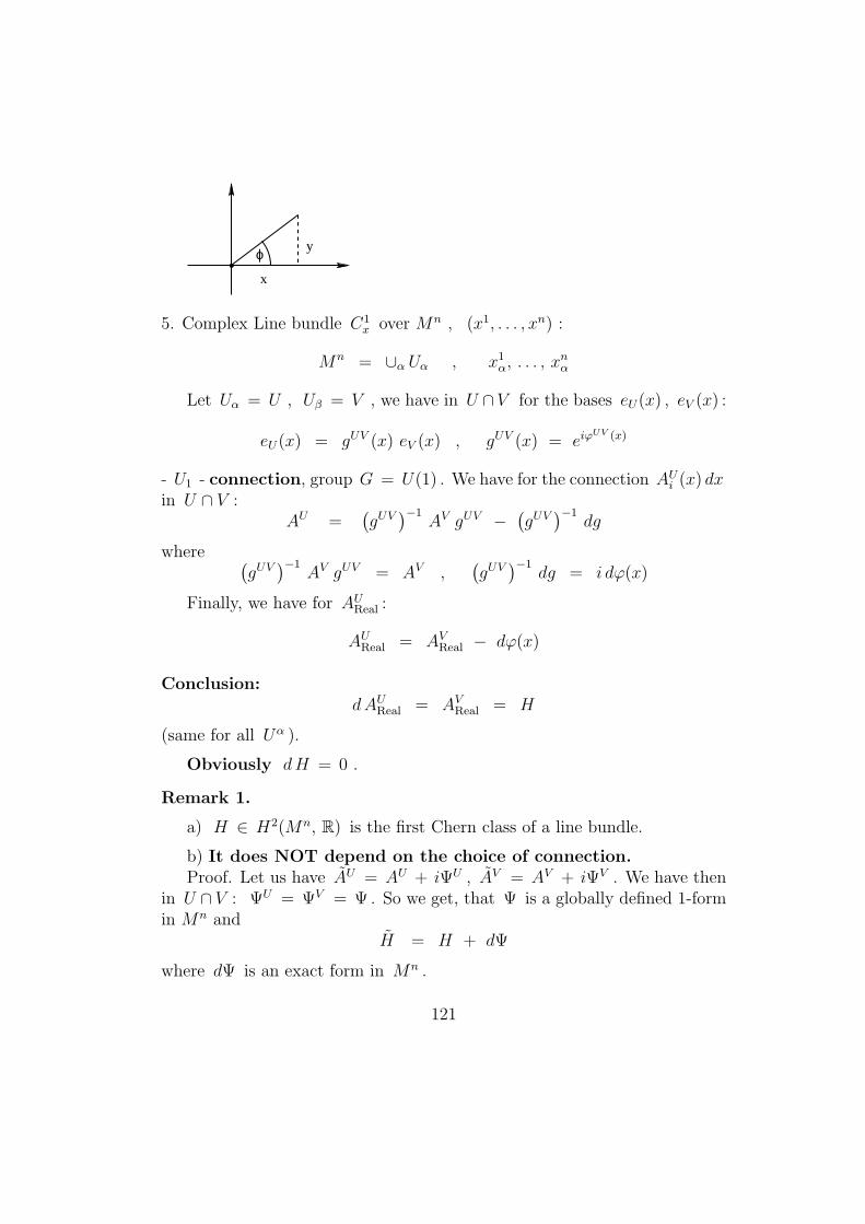
x
yϕ
5. Complex Line bundle C1x over Mn , (x1, . . . , xn) :
Mn = ∪α Uα , x1α, . . . , xnα
Let Uα = U , Uβ = V , we have in U ∩V for the bases eU(x) , eV (x) :
eU(x) = gUV (x) eV (x) , gUV (x) = eiφUV (x)
- U1 - connection, group G = U(1) . We have for the connection AUi (x) dxin U ∩ V :
AU =(gUV
)−1AV gUV −
(gUV
)−1dg
where (gUV
)−1AV gUV = AV ,
(gUV
)−1dg = i dφ(x)
Finally, we have for AUReal :
AUReal = AVReal − dφ(x)
Conclusion:dAUReal = AVReal = H
(same for all Uα ).
Obviously dH = 0 .
Remark 1.
a) H ∈ H2(Mn, R) is the first Chern class of a line bundle.
b) It does NOT depend on the choice of connection.Proof. Let us have AU = AU + iΨU , AV = AV + iΨV . We have then
in U ∩ V : ΨU = ΨV = Ψ . So we get, that Ψ is a globally defined 1-formin Mn and
H = H + dΨ
where dΨ is an exact form in Mn .
121
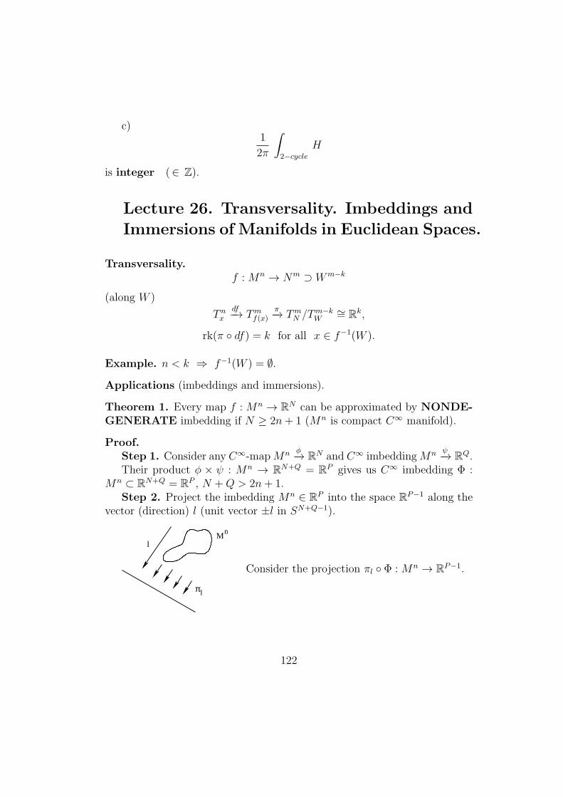
c)1
2π
∫2−cycle
H
is integer (∈ Z).
Lecture 26. Transversality. Imbeddings and
Immersions of Manifolds in Euclidean Spaces.
Transversality.f :Mn → Nm ⊃ Wm−k
(along W )
T nxdf−→ Tmf(x)
π−→ TmN /Tm−kW
∼= Rk,
rk(π df) = k for all x ∈ f−1(W ).
Example. n < k ⇒ f−1(W ) = ∅.
Applications (imbeddings and immersions).
Theorem 1. Every map f :Mn → RN can be approximated by NONDE-GENERATE imbedding if N ≥ 2n+ 1 (Mn is compact C∞ manifold).
Proof.Step 1. Consider any C∞-mapMn ϕ−→ RN and C∞ imbeddingMn ψ−→ RQ.Their product ϕ × ψ : Mn → RN+Q = RP gives us C∞ imbedding Φ :
Mn ⊂ RN+Q = RP , N +Q > 2n+ 1.Step 2. Project the imbedding Mn ∈ RP into the space RP−1 along the
vector (direction) l (unit vector ±l in SN+Q−1).
πl
Mn
l
Consider the projection πl Φ :Mn → RP−1.
122
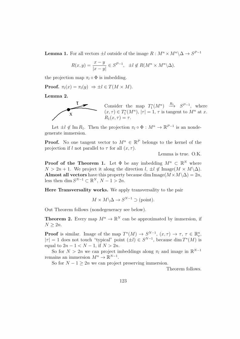
Lemma 1. For all vectors ±l outside of the image R :Mn×Mn\∆→ SP−1
R(x, y) =x− y|x− y|
∈ SP−1, ±l ∈ R(Mn ×Mn\∆).
the projection map πl Φ is imbedding.
Proof. πl(x) = πl(y) ⇒ ±l ∈ T (M ×M).
Lemma 2.
τ
x
Consider the map T ∗1 (M
n)R1−→ SP−1, where
(x, τ) ∈ T ∗1 (M
n), |τ | = 1, τ is tangent to Mn at x.R1(x, τ) = τ .
Let ±l ∈ ImR1. Then the projection πl Φ : Mn → RP−1 is an nonde-generate immersion.
Proof. No one tangent vector to Mn ∈ RP belongs to the kernel of theprojection if l not parallel to τ for all (x, τ).
Lemma is true. O.K.
Proof of the Theorem 1. Let Φ be any imbedding Mn ⊂ RN whereN > 2n + 1. We project it along the direction l, ±l ∈ Image(M ×M\∆).Almost all vectors have this property because dim Image(M×M\∆) = 2n,less then dimSN−1 ⊂ RN , N − 1 > 2n.
Here Transversality works. We apply transversality to the pair
M ×M\∆→ SN−1 ⊃ (point).
Out Theorem follows (nondegeneracy see below).
Theorem 2. Every map Mn → RN can be approximated by immersion, ifN ≥ 2n.
Proof is similar. Image of the map T ∗(M) → SN−1, (x, τ) → τ , τ ∈ Rnx,
|τ | = 1 does not touch “typical” point (±l) ∈ SN−1, because dimT ∗(M) isequal to 2n− 1 < N − 1, if N > 2n.
So for N > 2n we can project imbeddings along πl and image in RN−1
remains an immersion Mn → RN−1.So for N − 1 ≥ 2n we can project preserving immersion.
Theorem follows.
123
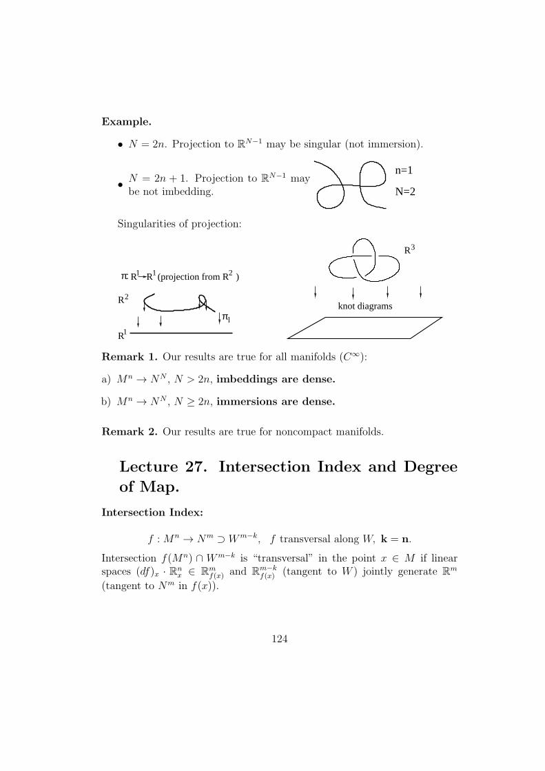
Example.
• N = 2n. Projection to RN−1 may be singular (not immersion).
• N = 2n + 1. Projection to RN−1 maybe not imbedding.
n=1
N=2
Singularities of projection:
π: 1 1
R
R2
1
R R (projection from R )2
πl
R3
knot diagrams
Remark 1. Our results are true for all manifolds (C∞):
a) Mn → NN , N > 2n, imbeddings are dense.
b) Mn → NN , N ≥ 2n, immersions are dense.
Remark 2. Our results are true for noncompact manifolds.
Lecture 27. Intersection Index and Degree
of Map.
Intersection Index:
f :Mn → Nm ⊃ Wm−k, f transversal along W, k = n.
Intersection f(Mn) ∩ Wm−k is “transversal” in the point x ∈ M if linearspaces (df)x · Rn
x ∈ Rmf(x) and Rm−k
f(x) (tangent to W ) jointly generate Rm
(tangent to Nm in f(x)).
124
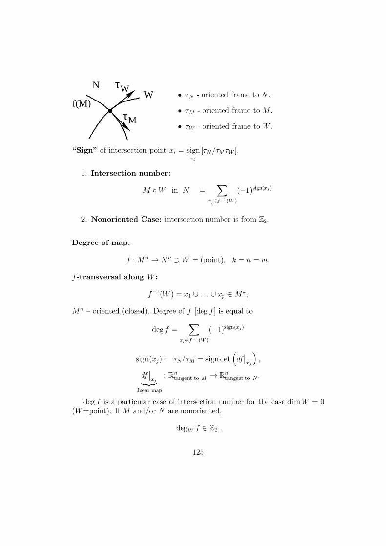
τM
τWW
f(M)
N• τN - oriented frame to N .
• τM - oriented frame to M .
• τW - oriented frame to W .
“Sign” of intersection point xi = signxj
[τN/τMτW ].
1. Intersection number:
M W in N =∑
xj∈f−1(W )
(−1)sign(xj)
2. Nonoriented Case: intersection number is from Z2.
Degree of map.
f :Mn → Nn ⊃ W = (point), k = n = m.
f-transversal along W :
f−1(W ) = x1 ∪ . . . ∪ xp ∈Mn,
Mn – oriented (closed). Degree of f [deg f ] is equal to
deg f =∑
xj∈f−1(W )
(−1)sign(xj)
sign(xj) : τN/τM = sign det(df∣∣xj
),
df∣∣xj︸︷︷︸
linear map
: Rntangent to M → Rn
tangent to N .
deg f is a particular case of intersection number for the case dimW = 0(W=point). If M and/or N are nonoriented,
degW f ∈ Z2.
125
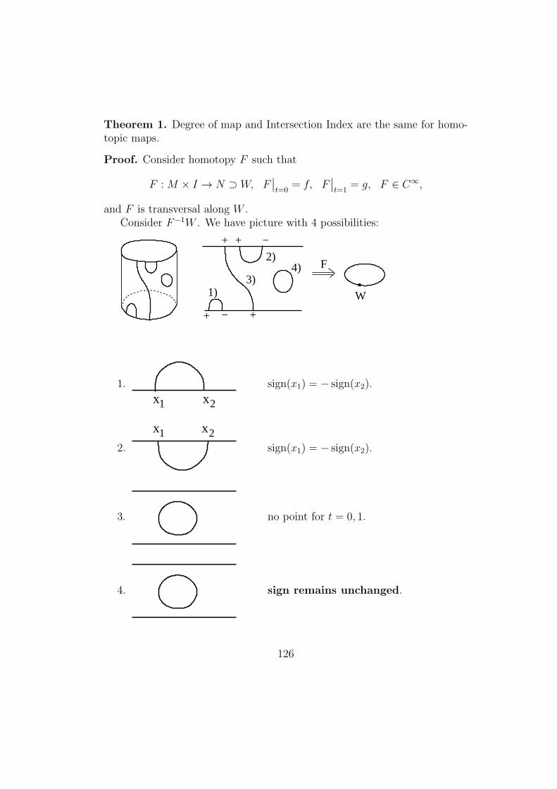
Theorem 1. Degree of map and Intersection Index are the same for homo-topic maps.
Proof. Consider homotopy F such that
F :M × I → N ⊃ W, F∣∣t=0
= f, F∣∣t=1
= g, F ∈ C∞,
and F is transversal along W .Consider F−1W . We have picture with 4 possibilities:
1)3)
2)4)
+
+ − +
+ −
F
W
1.
x1 x2
sign(x1) = − sign(x2).
2.
x2x1sign(x1) = − sign(x2).
3. no point for t = 0, 1.
4. sign remains unchanged.
126
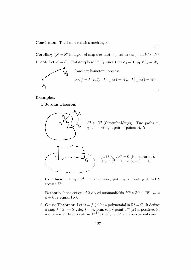
Conclusion. Total sum remains unchanged.O.K.
Corollary (N = Sn): degree of map does not depend on the pointW ⊂ Nn.
Proof. Let N = Sn. Rotate sphere Sn ϕt, such that ϕ0 = 1, ϕ1(W1) = W2,
W1
W2Consider homotopy process
ϕt f = F (x, t), F∣∣t=o
(x) = W1, F∣∣t=1
(x) = W2.
O.K.
Examples.
1. Jordan Theorem.
B
Aγ1
γ2S1 ⊂ R2 (C∞-imbeddings). Two paths γ1,γ2 connecting a pair of points A, B.
γ1 γ
2
(γ1 ∪ γ2) S1 = 0 (Homework 9).If γ1 S1 = 1 ⇒ γ2 S1 = ±1.
Conclusion. If γ1 S1 = 1, then every path γ2 connecting A and Bcrosses S1.
Remark. Intersection of 2 closed submanifolds Mn W k ∈ Rm, m =n+ k is equal to 0.
2. Gauss Theorem: Let w = fn(z) be a polynomial in R2 = C. It definesa map f : S2 → S2, deg f = n, plus every point f−1(w) is positive. Sowe have exactly n points in f−1(w) : z1, . . . , zn in transversal case.
127
3. F : Mn → Nn – map of closed oriented manifolds, m = n = k, W -point.
Theorem. ∫M
f ∗(Ω) = (deg f)︸ ︷︷ ︸integer
∫N
Ω, (Why?)
Application in Geometry will be presented.
Lecture 28. Intersection Index and Degree
of Map.
Intersection index and degree of map are homotopy invariant.
Theorem. Let Mn, Nn be oriented (closed) manifolds and f : Mn → Nn
be a C∞-map. Then for every n-form Ω in N we have∫M
f ∗(Ω) = (deg f)︸ ︷︷ ︸integer
·∫N
Ω.
Proof. By transversality theorem, almost all points W ∈ N are “transver-sal” along W ∈ N . The set of transversal points in N is open and has mea-sure=1. So the integral
∫N
Ω depends only on the set of transversal points in
w ∈ N . Let U ∋ w be a small open set containing w such that all points inU are transversal. Let U be connected set.
We have f−1(U) = U1 ∪ . . . ∪ Ul where Ujf−→ U is a diffeomorphism
preserving (+) or reversing (−) orientation with sign = (−1)sj , j = 1, . . . , l.We have ∫
Uj
f ∗Ω = (−1)sj∫U
Ω,
and ∫f−1(U)
f ∗Ω =
∫U
Ω
·(∑j
(−1)sj).
128
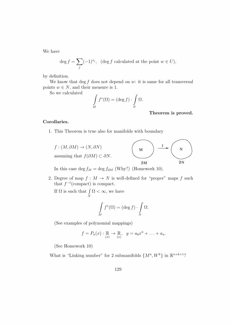
We have
deg f =∑j
(−1)sj , (deg f calculated at the point w ∈ U),
by definition.We know that deg f does not depend on w: it is same for all transversal
points w ∈ N , and their measure is 1.So we calculated ∫
M
f ∗(Ω) = (deg f) ·∫N
Ω.
Theorem is proved.
Corollaries.
1. This Theorem is true also for manifolds with boundary
f : (M,∂M)→ (N, ∂N)
assuming that f(∂M) ⊂ ∂N .
fM N
M N
In this case deg fM = deg f∂M (Why?) (Homework 10).
2. Degree of map f : M → N is well-defined for “proper” maps f suchthat f−1(compact) is compact.
If Ω is such that∫N
Ω <∞, we have
∫M
f ∗(Ω) = (deg f) ·∫N
Ω.
(See examples of polynomial mappings)
f = Pn(x) : R(x)→ R
(x), y = a0x
n + . . .+ an.
(See Homework 10)
What is “Linking number” for 2 submanifolds Mn,W k in Rn+k+1?
129
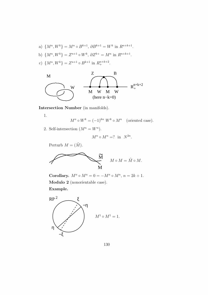
a) Mn,W k =Mn Bk+1, ∂Bk+1 = W k in Rn+k+1.
b) Mn,W k = Zn+1 W k, ∂Zk+ =Mn in Rn+k+1.
c) Mn,W k = Zn+1 Bk+1 in Rn+k+2+ .
R+n+k+2
M
WM
(here n−k=0)MW W
Z B
Intersection Number (in manifolds).
1.Mn W k = (−1)kn W k Mn (oriented case).
2. Self-intersection (Mn = W n).
Mn Mn =? in N2n.
Perturb M = (M).
M
MM M = M M .
Corollary. Mn Mn = 0 = −Mn Mn, n = 2k + 1.
Modulo 2 (nonorientable case).
Example.
RP 2
−ξη
−ηξ
M1 M1 = 1.
130
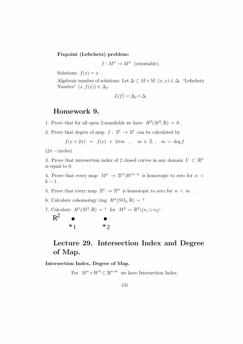
Fixpoint (Lefschetz) problem:
f :Mn →Mn (orientable).
Solutions: f(x) = x.
Algebraic number of solutions: Let ∆ ⊂M×M , (x, x) ∈ ∆. “LefschetzNumber” (x, f(x)) ∈ ∆f .
L(f) = ∆f ∆.
Homework 9.
1. Prove that for all open 2-manifolds we have H2(M2,R) = 0 .
2. Prove that degree of map f : S1 → S1 can be calculated by
f(x+ 2π) = f(x) + 2πm , m ∈ Z , m = deg f
(2π - circles).
3. Prove that intersection index of 2 closed curves in any domain U ⊂ R2
is equal to 0.
4. Prove that every map Mn → Sm\Wm−k is homotopic to zero for n <k − 1 .
5. Prove that every map Sn → Sm is homotopic to zero for n < m .
6. Calculate cohomology ring H∗(SO4,R) = ?
7. Calculate H1(M2,R) = ? for M2 = R2\(∗1 ∪ ∗2) :
R2
* *21
Lecture 29. Intersection Index and Degree
of Map.
Intersection Index, Degree of Map.
For Mn W k ⊂ Rn+k we have Intersection Index.
131
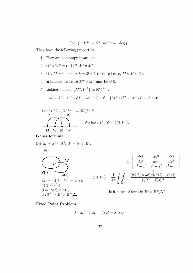
For f :Mn → Nn we have deg f.
They have the following properties:
1. They are homotopy invariant.
2. Mn W k = (−1)kn W k Mn.
3. M M = 0 for n = k = 2l + 1 (oriented case, M M ∈ Z).
4. In nonoriented case Mn Mn may be = 0.
5. Linking number Mn,W k in Rn+k+1.
M = ∂Z, W = ∂B, M ∩W = ∅, Mn,W k =M B = Z W.
Let M,W ∈ Rn+k+1 = ∂Rn+k+2+
M MW W
Z B
We have B Z = M,W.
Gauss formula:
Let M = S1 ∈ R3, W = S1 ∈ R3.
γ(t)
M
W
x(s)
M = γ(t), W = x(s),γ(t) = x(s),ϕ = γ(t), x(s),ϕ : T 2 → R3 × R3\∆.
M,W = 1
4π
∮M
∮W
det
∣∣∣∣∣∣dγ1 dγ2 dγ3
dx1 dx2 dx3
γ1 − x1 γ2 − x2 γ3 − x3
∣∣∣∣∣∣∥
(dγ(t)× dx(s), γ(t)− x(s))|γ(t)− x(s)|3
Is it closed 2-form in R3 × R3\∆?
Fixed Point Problem.
f :Mn →Mn, f(x) = x (?)
132
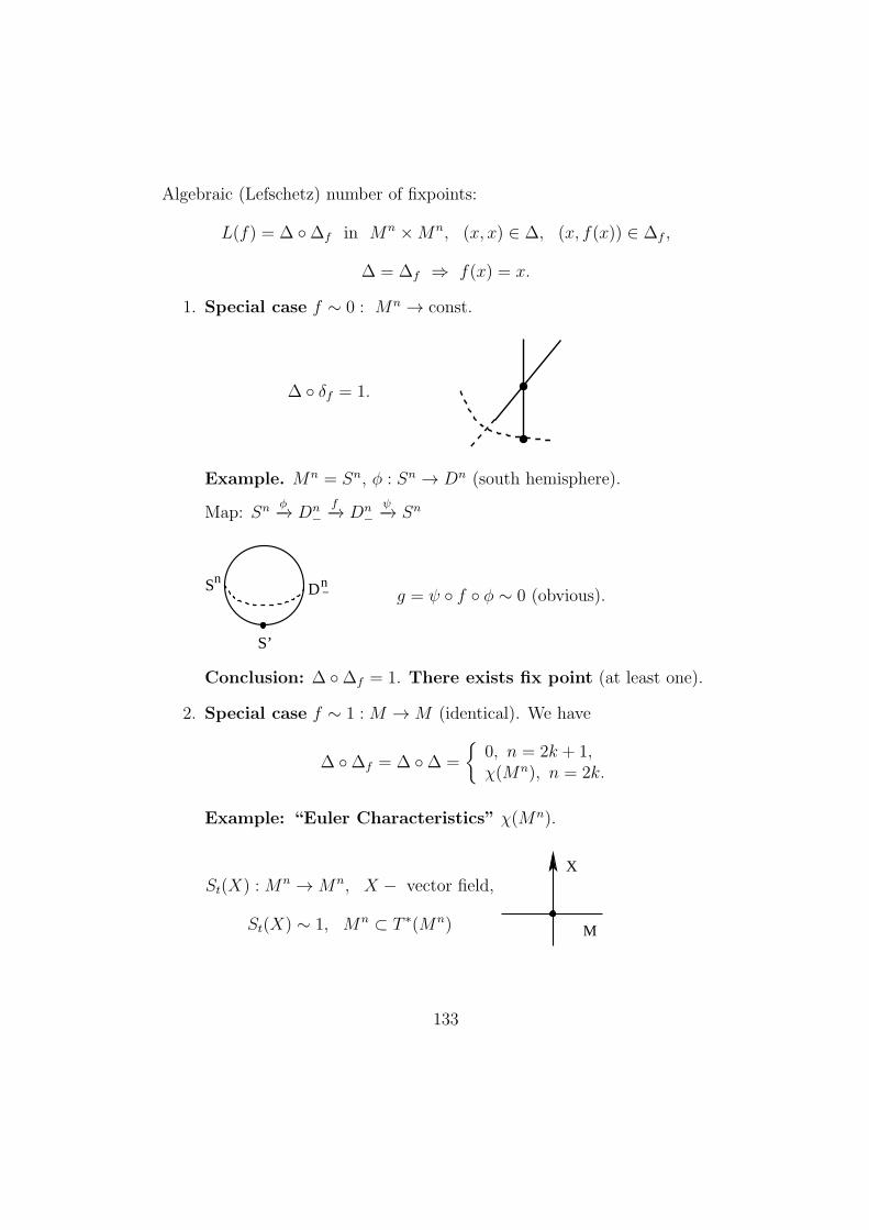
Algebraic (Lefschetz) number of fixpoints:
L(f) = ∆ ∆f in Mn ×Mn, (x, x) ∈ ∆, (x, f(x)) ∈ ∆f ,
∆ = ∆f ⇒ f(x) = x.
1. Special case f ∼ 0 : Mn → const.
∆ δf = 1.
Example. Mn = Sn, ϕ : Sn → Dn (south hemisphere).
Map: Snϕ−→ Dn
−f−→ Dn
−ψ−→ Sn
SnDn
−
S’
g = ψ f ϕ ∼ 0 (obvious).
Conclusion: ∆ ∆f = 1. There exists fix point (at least one).
2. Special case f ∼ 1 :M →M (identical). We have
∆ ∆f = ∆ ∆ =
0, n = 2k + 1,χ(Mn), n = 2k.
Example: “Euler Characteristics” χ(Mn).
St(X) :Mn →Mn, X − vector field,
St(X) ∼ 1, Mn ⊂ T ∗(Mn) M
X
133
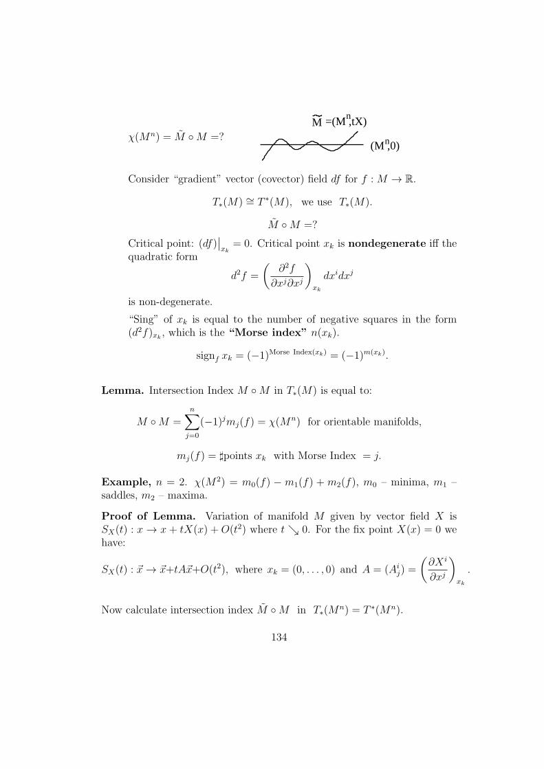
χ(Mn) = M M =?
M
(M ,0)
=(M ,tX)n
n
Consider “gradient” vector (covector) field df for f :M → R.
T∗(M) ∼= T ∗(M), we use T∗(M).
M M =?
Critical point: (df)∣∣xk
= 0. Critical point xk is nondegenerate iff thequadratic form
d2f =
(∂2f
∂xj∂xj
)xk
dxidxj
is non-degenerate.
“Sing” of xk is equal to the number of negative squares in the form(d2f)xk , which is the “Morse index” n(xk).
signf xk = (−1)Morse Index(xk) = (−1)m(xk).
Lemma. Intersection Index M M in T∗(M) is equal to:
M M =n∑j=0
(−1)jmj(f) = χ(Mn) for orientable manifolds,
mj(f) = ♯points xk with Morse Index = j.
Example, n = 2. χ(M2) = m0(f) − m1(f) + m2(f), m0 – minima, m1 –saddles, m2 – maxima.
Proof of Lemma. Variation of manifold M given by vector field X isSX(t) : x→ x + tX(x) + O(t2) where t 0. For the fix point X(x) = 0 wehave:
SX(t) : x→ x+tAx+O(t2), where xk = (0, . . . , 0) and A = (Aij) =
(∂X i
∂xj
)xk
.
Now calculate intersection index M M in T∗(Mn) = T ∗(Mn).
134
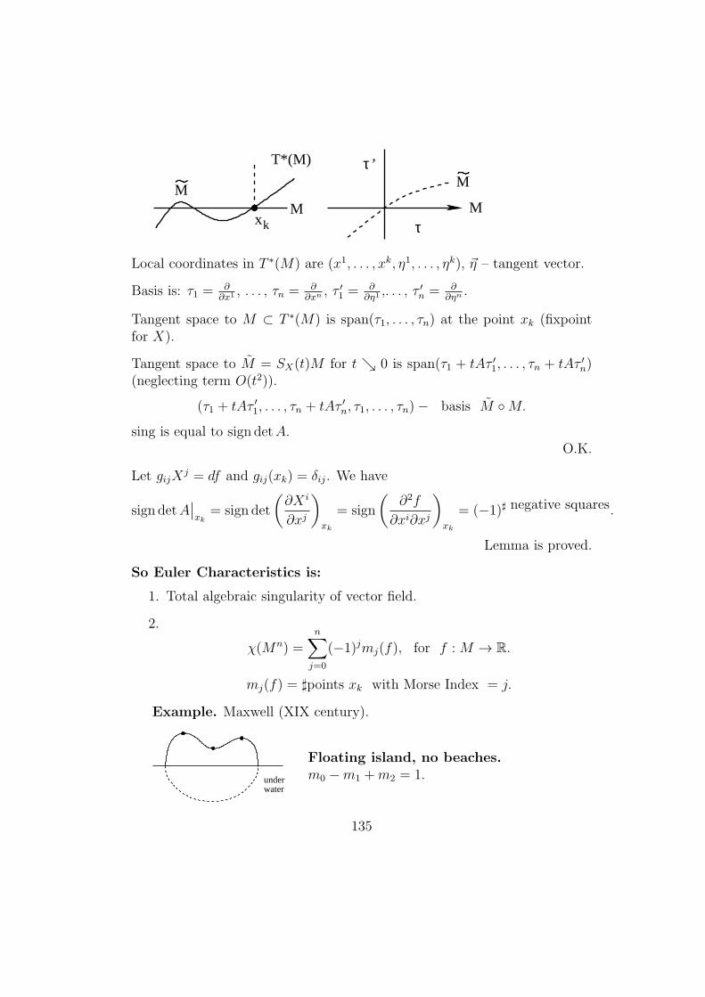
M Mτ ’
xkM M
τ
T*(M)
Local coordinates in T ∗(M) are (x1, . . . , xk, η1, . . . , ηk), η – tangent vector.
Basis is: τ1 =∂∂x1
, . . . , τn = ∂∂xn
, τ ′1 =∂∂η1
,. . . , τ ′n = ∂∂ηn
.
Tangent space to M ⊂ T ∗(M) is span(τ1, . . . , τn) at the point xk (fixpointfor X).
Tangent space to M = SX(t)M for t 0 is span(τ1 + tAτ ′1, . . . , τn + tAτ ′n)(neglecting term O(t2)).
(τ1 + tAτ ′1, . . . , τn + tAτ ′n, τ1, . . . , τn)− basis M M.
sing is equal to sign detA.O.K.
Let gijXj = df and gij(xk) = δij. We have
sign detA∣∣xk
= sign det
(∂X i
∂xj
)xk
= sign
(∂2f
∂xi∂xj
)xk
= (−1)♯ negative squares.
Lemma is proved.
So Euler Characteristics is:
1. Total algebraic singularity of vector field.
2.
χ(Mn) =n∑j=0
(−1)jmj(f), for f :M → R.
mj(f) = ♯points xk with Morse Index = j.
Example. Maxwell (XIX century).
underwater
Floating island, no beaches.m0 −m1 +m2 = 1.
135
Lecture 30. Two applications of differential
forms: Degree of Map and Hopf Invariant.
Two applications of differential forms.
I) Homotopy theory: Degree of map Snf−→ Sn (spheres may be replaced
by any closed orientable manifolds:)
A) Take n-form Ω ∈ ∧n(Sn),∫Sn
Ω = 1.
Definition.
deg f =
∫Sn
f ∗(Ω)
Proof.
Let F be a homotopy from f to g: F : Sn×I → Sn, (0 ≤ t ≤ 1), F (x, 0) =f , F (x, 1) = g. Consider F ∗(Ω)). We have dF ∗(Ω) = F ∗(dΩ) = 0.∫
(Sn,1)
F ∗(Ω)xg∗Ω
−∫
(Sn,0)
F ∗(Ω)xf ∗Ω
=
∫(Sn×I)
dF ∗(Ω) = 0.
Ω→ Ω + dω ⇒∫
(Sn,t)
Ω + dω =
∫(Sn,t)
Ω.
Theorem is proved.
We calculated integral∫Sn
f ∗Ω geometrically and proved geometrically
that∫Sn
f ∗Ω =
(∫Sn
Ω
)· deg f .
B) Consider S3 → S2 and fix 2-form Ω in ∧2(S2) such that∫S2
Ω = 1.
Let f ∗Ω = dω, ω ∈ ∧1(S3).
Define “Hopf Invariant”
H(f) =
∫S3
ω ∧ f ∗Ω.
136
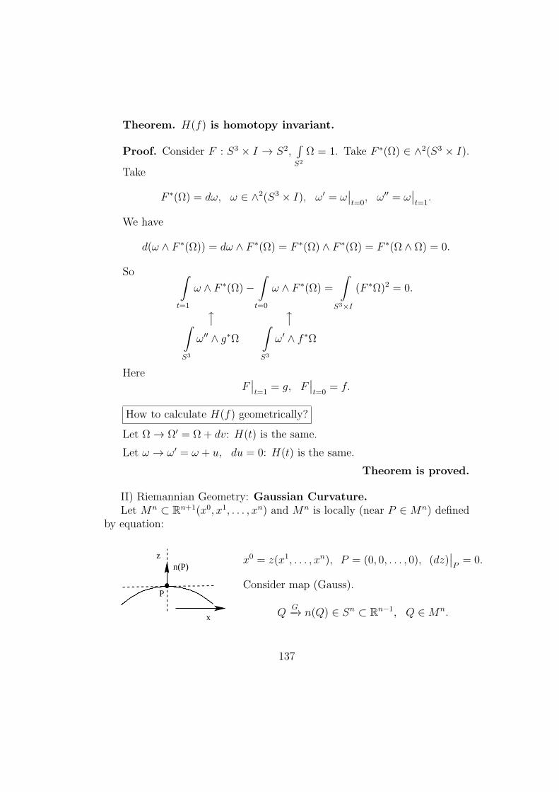
Theorem. H(f) is homotopy invariant.
Proof. Consider F : S3 × I → S2,∫S2
Ω = 1. Take F ∗(Ω) ∈ ∧2(S3 × I).
Take
F ∗(Ω) = dω, ω ∈ ∧2(S3 × I), ω′ = ω∣∣t=0, ω′′ = ω
∣∣t=1.
We have
d(ω ∧ F ∗(Ω)) = dω ∧ F ∗(Ω) = F ∗(Ω) ∧ F ∗(Ω) = F ∗(Ω ∧ Ω) = 0.
So ∫t=1
ω ∧ F ∗(Ω)x∫S3
ω′′ ∧ g∗Ω
−∫t=0
ω ∧ F ∗(Ω)x∫S3
ω′ ∧ f ∗Ω
=
∫S3×I
(F ∗Ω)2 = 0.
HereF∣∣t=1
= g, F∣∣t=0
= f.
How to calculate H(f) geometrically?
Let Ω→ Ω′ = Ω+ dv: H(t) is the same.
Let ω → ω′ = ω + u, du = 0: H(t) is the same.
Theorem is proved.
II) Riemannian Geometry: Gaussian Curvature.Let Mn ⊂ Rn+1(x0, x1, . . . , xn) and Mn is locally (near P ∈Mn) defined
by equation:
zn(P)
P
x
x0 = z(x1, . . . , xn), P = (0, 0, . . . , 0), (dz)∣∣P= 0.
Consider map (Gauss).
QG−→ n(Q) ∈ Sn ⊂ Rn−1, Q ∈Mn.
137
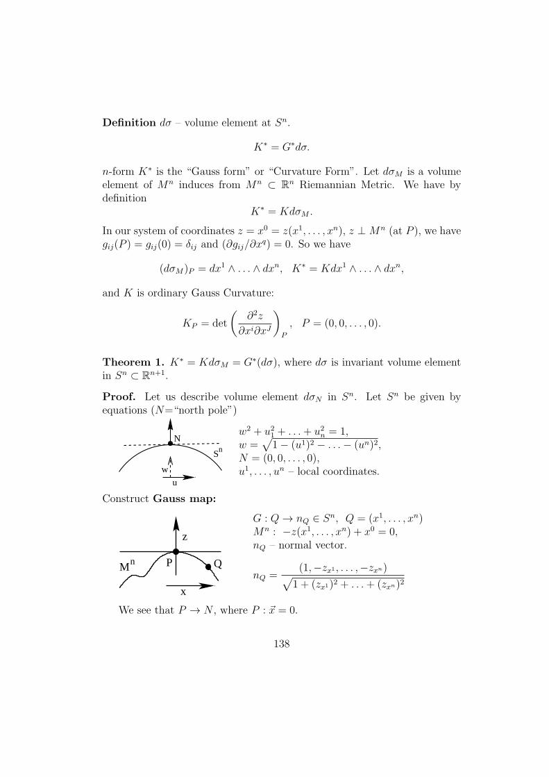
Definition dσ – volume element at Sn.
K∗ = G∗dσ.
n-form K∗ is the “Gauss form” or “Curvature Form”. Let dσM is a volumeelement of Mn induces from Mn ⊂ Rn Riemannian Metric. We have bydefinition
K∗ = KdσM .
In our system of coordinates z = x0 = z(x1, . . . , xn), z ⊥Mn (at P ), we havegij(P ) = gij(0) = δij and (∂gij/∂x
q) = 0. So we have
(dσM)P = dx1 ∧ . . . ∧ dxn, K∗ = Kdx1 ∧ . . . ∧ dxn,
and K is ordinary Gauss Curvature:
KP = det
(∂2z
∂xi∂xJ
)P
, P = (0, 0, . . . , 0).
Theorem 1. K∗ = KdσM = G∗(dσ), where dσ is invariant volume elementin Sn ⊂ Rn+1.
Proof. Let us describe volume element dσN in Sn. Let Sn be given byequations (N=“north pole”)
Sn
u
w
Nw2 + u21 + . . .+ u2n = 1,w =
√1− (u1)2 − . . .− (un)2,
N = (0, 0, . . . , 0),u1, . . . , un – local coordinates.
Construct Gauss map:
Mn Q
z
x
P
G : Q→ nQ ∈ Sn, Q = (x1, . . . , xn)Mn : −z(x1, . . . , xn) + x0 = 0,nQ – normal vector.
nQ =(1,−zx1 , . . . ,−zxn)√
1 + (zx1)2 + . . .+ (zxn)2
We see that P → N , where P : x = 0.
138
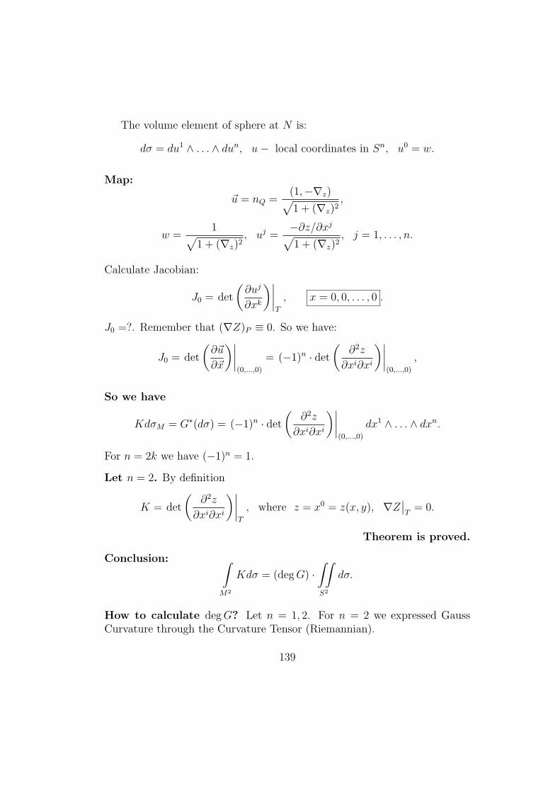
The volume element of sphere at N is:
dσ = du1 ∧ . . . ∧ dun, u− local coordinates in Sn, u0 = w.
Map:
u = nQ =(1,−∇z)√1 + (∇z)2
,
w =1√
1 + (∇z)2, uj =
−∂z/∂xj√1 + (∇z)2
, j = 1, . . . , n.
Calculate Jacobian:
J0 = det
(∂uj
∂xk
)∣∣∣∣T
, x = 0, 0, . . . , 0 .
J0 =?. Remember that (∇Z)P ≡ 0. So we have:
J0 = det
(∂u
∂x
)∣∣∣∣(0,...,0)
= (−1)n · det(
∂2z
∂xi∂xi
)∣∣∣∣(0,...,0)
,
So we have
KdσM = G∗(dσ) = (−1)n · det(
∂2z
∂xi∂xi
)∣∣∣∣(0,...,0)
dx1 ∧ . . . ∧ dxn.
For n = 2k we have (−1)n = 1.
Let n = 2. By definition
K = det
(∂2z
∂xi∂xi
)∣∣∣∣T
, where z = x0 = z(x, y), ∇Z∣∣T= 0.
Theorem is proved.
Conclusion: ∫M2
Kdσ = (degG) ·∫∫S2
dσ.
How to calculate degG? Let n = 1, 2. For n = 2 we expressed GaussCurvature through the Curvature Tensor (Riemannian).
139
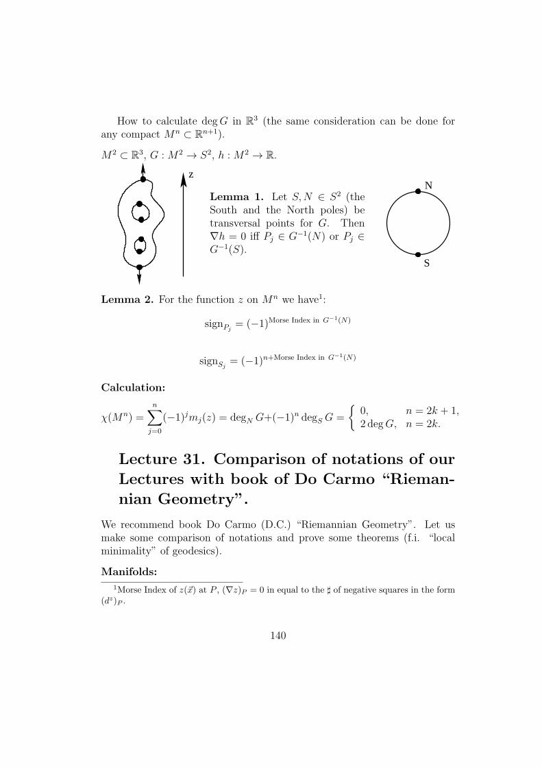
How to calculate degG in R3 (the same consideration can be done forany compact Mn ⊂ Rn+1).
M2 ⊂ R3, G :M2 → S2, h :M2 → R.
z
Lemma 1. Let S,N ∈ S2 (theSouth and the North poles) betransversal points for G. Then∇h = 0 iff Pj ∈ G−1(N) or Pj ∈G−1(S).
N
S
Lemma 2. For the function z on Mn we have1:
signPj= (−1)Morse Index in G−1(N)
signSj= (−1)n+Morse Index in G−1(N)
Calculation:
χ(Mn) =n∑j=0
(−1)jmj(z) = degN G+(−1)n degS G =
0, n = 2k + 1,2 degG, n = 2k.
Lecture 31. Comparison of notations of our
Lectures with book of Do Carmo “Rieman-
nian Geometry”.
We recommend book Do Carmo (D.C.) “Riemannian Geometry”. Let usmake some comparison of notations and prove some theorems (f.i. “localminimality” of geodesics).
Manifolds:
1Morse Index of z(x) at P , (∇z)P = 0 in equal to the ♯ of negative squares in the form(dz)P .
140
D.C. “Differential Structure”, Hausdorff.
Our Course: “Atlas of Charts”, C∞ manifolds, metric spaces, “Dou-ble good Atlas”.
Local coordinates - same.
Imbedding and Immersions Mn = RN (proof of existence is missing inD.C.).
Partition of unity (proof is missing in D.C.) - we proved for compactmanifolds.
Tangent vectors, basis of T nτ as ∂i = ∂/∂xi in local coordinates(x1, . . . , xn) .
Vector field X =∑
ai(x) ∂i (locally).
Our notation X = (ai) (index is “upper”). Action of vector field onfunctions f(x) :
D.C. : X (f) =∑
ai(x)∂f
∂xi= ai
∂f
∂xi
Commutator[X , Y ] = X (Y (t)) − Y (X(t))
X = (ai) , Y = (bi) , [X , Y ]i =
(aj∂bi
∂xj− bj
∂ai
∂xj
)C∞-maps : Mn f−→ Nm , differential of map, rank :
d fτ : T nτ → Tmf(τ) (linear)
Implicit function theorem / local inversion theorem of the map (no proofin D.C. and in our course).
Approximation and Transversality are missing in D.C. or presented in thehighly reduced form - see C.P.
Examples of manifolds - similar.
Orientation.
Covectors (basis (dxi) in local coordinates) are missing in D.C. Covectorfields ω =
∑i ui(x) dx
i (1-forms).
Manifolds T ∗(Mn) (vectors), Atlas, Charts.
Manifolds T∗(Mn) (covectors, missing in D.C.)
141
Riemannian and Pseudoriemannian Metric = inner product (symmetric,nondegenerate) is ⟨X , Y ⟩ , gij = ⟨∂i , ∂j⟩ .
Symplectic inner products and differential forms are missing inD.C.
Volume element dn σ =√
det gij dx1 ∧ · · · ∧ dxn (locally).
Induced Metric for submanifolds Mn ⊂ RN or Mn ⊂ Nk (good onlyfor positive Riemannian Metrics).
Lie Groups, right and left invariant vector fields, right and left invariantRiemannian Metric on Compact Lie Groups, bi-invariant metric and innerproduct of right-invariant vector fields (D.C.).
Riemannian Metric and length of curves. Existence of Riemannian metricin every manifold (proved by partition of unity in D.C.; another proof -imbedding in RN). Volume provided by Riemannian metric.
Existence of biinvariant volume on a compact group G. Existence ofinvariant metric in the spaces with action of compact group G (“averagingprocedure” - both in D.C. and our course).
Connections (“affine”) - considered in D.C. for tangent bundles only:vector field X, X = ai(x) ∂i ,
∇X Y =∑i
ai∇i Y , Y = bj(x) ∂j
∇i Y = bj (∇i ∂j) +∂bj
∂xi∂j =
(∂bj
∂xi+ bj Γkij
)∂j
for components, ∇i(∂j) = Γkij ∂k .
Symmetric Connection” Γkij = Γkji ∇i ∂j = ∇j ∂i .Curve
c(t) = xj(t) , X = (x)
Let V be a vector fields, V = (vj) , X(t) - tangent to c.
d
dt(V ) = ∇X V =
(dvj
dt+ vq xk Γjqk
)∂k
D.C. : Xj ↔ ∂j , ∇XiXj = Γkij ∂k , X = (xj(t)) along c(t) .
Tensors. Examples:
142
1. Scalars (type (0, 0)) - f(x) .
2. Vectors (type (1, 0)) - (ui)∑
ui ∂i .
3. Covectors (type (0, 1)) - (vi)∑
vi dxi .
4. Inner products of vectors gij (type (0, 2)) .
5. Inner products of covectors gij (type (2, 0)) .
6. Operators (aij) (type (1, 1)) .
General Tensors (type (k, l)) .
Components T i1...ikj1...jl(x)
e1, . . . , en - basis of tangent vectors
e1, . . . , en - basis of covectors
ei1 ⊗ ei2 ⊗ . . . ⊗ eik ⊗ ej1 ⊗ ej2 ⊗ . . . ⊗ ejl - basis in tensor space(k, l).
Operations : Linear, Tensor product
(k, l) ⊗ (p, q) ⊂ (k + p, l + q)
T ′i′j′ ⊗ T ′i′′
j′′ = T i′i′′
j′j′′(x)
Permutation of indices (lower or upper)
Trace
T i′ i i′′
j′jj′′Trace−−−→ T i
′ i′′
j′ j′′ =n∑i=1
T i′ i i′′
j′ i j′′
Examples: A = (aij) , aij → aij = TrA (trace), gij → gji - permuta-tion.
Extension of connection to all tensor fields. Axioms.
a) Trivial for scalar fields ∇i f = ∂i f .
b) Satisfies to Leibnitz formula for tensor products.
c) Annihilates Riemannian metric ∇i gkl ≡ 0 .
d) Commutes with trace
∇X ⟨V , W ⟩ = ui∂
∂xi⟨V , W ⟩ = ⟨∇X V , W ⟩ + ⟨V , ∇XW ⟩
143
where X = (ui) ,
∇k ⟨V , W ⟩ = ∇k
(gij v
iwj)
= ⟨∇k V , W ⟩ + ⟨V , ∇kW ⟩
∇k = ∇Xk, Xk = ∂k.
For parallel Transform
d
dt⟨V , W ⟩ = ⟨dV
dt, W ⟩ + ⟨V ,
dW
dt⟩
dV
dt= 0 ,
dW
dt= 0 ⇒ d⟨V , W ⟩
dt= 0
Levi - Civita Theorem. Symmetric connection compatible with metricgij is given by the formula
Γpjk =1
2gpi(∂gij∂xk
+∂gik∂xj
− ∂gjk∂xi
)“symmetric”: ∇k ∂j = ∇j ∂k ↔ ∇X Y − ∇Y X = [X , Y ] .
Homework 10.
1. Prove that for complex polynomial
w = Pn(z) : S2 → S2
we have deg f = n .
2. Calculate degree of rational map
w =Pn(z)
Qk(z), (irreducible fraction)
3. Calculate degree of real polynomial
y = a0 xn + a1 x
n−1 + . . . + an : R → R , aj ∈ R
4. Let γ(t) = γ(t+ 2π) : S1 → R2 and γ = 0 .
144
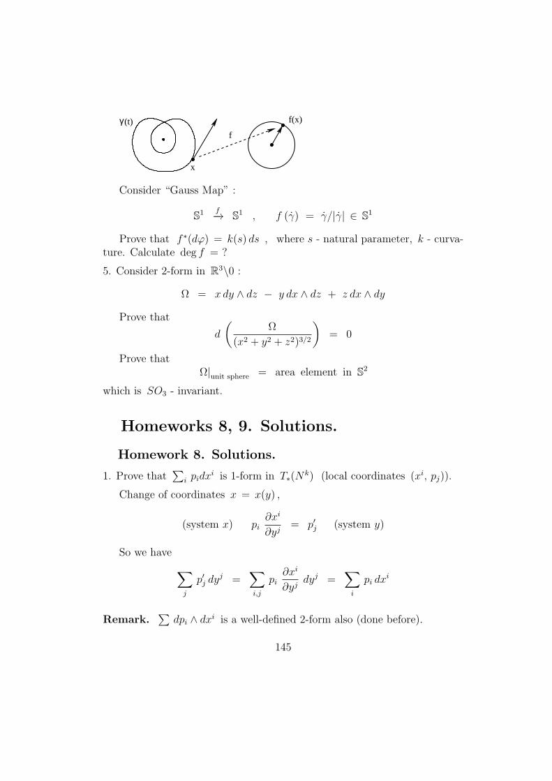
γ(t)
x
f(x)
f
Consider “Gauss Map” :
S1 f−→ S1 , f (γ) = γ/|γ| ∈ S1
Prove that f ∗(dφ) = k(s) ds , where s - natural parameter, k - curva-ture. Calculate deg f = ?
5. Consider 2-form in R3\0 :
Ω = x dy ∧ dz − y dx ∧ dz + z dx ∧ dy
Prove that
d
(Ω
(x2 + y2 + z2)3/2
)= 0
Prove thatΩ|unit sphere = area element in S2
which is SO3 - invariant.
Homeworks 8, 9. Solutions.
Homework 8. Solutions.
1. Prove that∑
i pidxi is 1-form in T∗(N
k) (local coordinates (xi, pj)).
Change of coordinates x = x(y) ,
(system x) pi∂xi
∂yj= p′j (system y)
So we have ∑j
p′j dyj =
∑i,j
pi∂xi
∂yjdyj =
∑i
pi dxi
Remark.∑
dpi ∧ dxi is a well-defined 2-form also (done before).
145
2. Prove that geodesic flow with Hamiltonian H(x, p) = gij(x) pi pj / 2preserves the form
∑i pi dx
i [correction due to student: it preserves theform
∑i pi dx
i restricted to the (2n−1) - dimensional submanifold T1(Mn) ,
|x| = 1 (unit tangent vectors)].
Proof. Calculation shows that for the shift St along the flow we have forgeodesic flow
d
dtS∗t
(∑i
pi dxi
)∣∣∣∣∣t=0
= dH
For geodesic flow have
H(x, p) =1
2gij(x) pi pj =
1
2gij(x) x
i xj
so T1(Mn) is given by the condition H = 1 and dH = 0 on T1(M
n) .
Calculation: We have
S∗t (pi) = pi + t pi + O(t2) , S∗
t (xi) = xi + t xi + O(t2)
For xi = Hpi , pi = −Hxi we have then
d
dtS∗t (pi)
∣∣∣∣t=0
= −Hxi ,d
dtS∗t (x
i)
∣∣∣∣t=0
= Hpi
d
dtS∗t (dx
i)
∣∣∣∣t=0
= dHpi = Hpipj dpj + Hpixj dxj
Finally:
d
dtS∗t
(∑i
pi dxi
)∣∣∣∣∣t=0
= −Hxi dxi + pi
[Hpipj dpj + Hpixj dx
j]
=
= d
(pi∂H
∂pi− H
)= dL
where L is a “Lagrangian”.For
H(x, p) =1
2gij(x) pi pj =
1
2gij(x) x
i xj
we have H = L and also dH = dL .
146
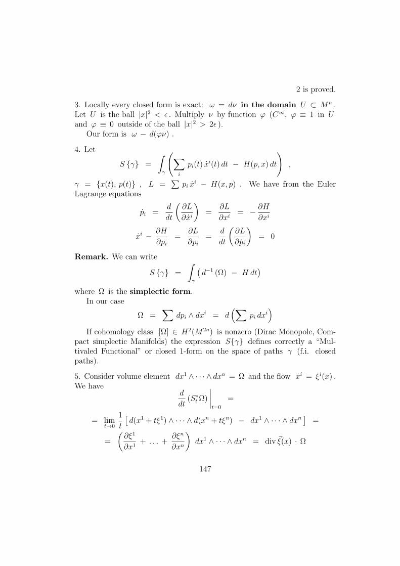
2 is proved.
3. Locally every closed form is exact: ω = dν in the domain U ⊂ Mn .Let U is the ball |x|2 < ϵ . Multiply ν by function φ (C∞, φ ≡ 1 in Uand φ ≡ 0 outside of the ball |x|2 > 2ϵ ).
Our form is ω − d(φν) .
4. Let
S γ =
∫γ
(∑i
pi(t) xi(t) dt − H(p, x) dt
),
γ = x(t), p(t) , L =∑
pi xi − H(x, p) . We have from the Euler
Lagrange equations
pi =d
dt
(∂L
∂xi
)=
∂L
∂xi= − ∂H
∂xi
xi − ∂H
∂pi=
∂L
∂pi=
d
dt
(∂L
∂pi
)= 0
Remark. We can write
S γ =
∫γ
(d−1 (Ω) − H dt
)where Ω is the simplectic form.
In our case
Ω =∑
dpi ∧ dxi = d(∑
pi dxi)
If cohomology class [Ω] ∈ H2(M2n) is nonzero (Dirac Monopole, Com-pact simplectic Manifolds) the expression Sγ defines correctly a “Mul-tivaled Functional” or closed 1-form on the space of paths γ (f.i. closedpaths).
5. Consider volume element dx1 ∧ · · · ∧ dxn = Ω and the flow xi = ξi(x) .We have
d
dt(S∗
tΩ)
∣∣∣∣t=0
=
= limt→0
1
t
[d(x1 + tξ1) ∧ · · · ∧ d(xn + tξn) − dx1 ∧ · · · ∧ dxn
]=
=
(∂ξ1
∂x1+ . . . +
∂ξn
∂xn
)dx1 ∧ · · · ∧ dxn = div ξ(x) · Ω
147
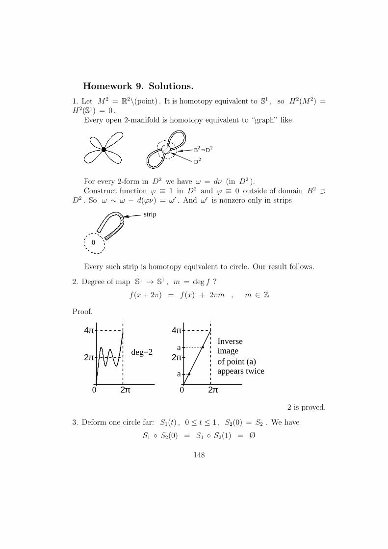
Homework 9. Solutions.
1. Let M2 = R2\(point) . It is homotopy equivalent to S1 , so H2(M2) =H2(S1) = 0 .
Every open 2-manifold is homotopy equivalent to “graph” like
B2 D2
D2
For every 2-form in D2 we have ω = dν (in D2 ).Construct function φ ≡ 1 in D2 and φ ≡ 0 outside of domain B2 ⊃
D2 . So ω ∼ ω − d(φν) = ω′ . And ω′ is nonzero only in strips
0
strip
Every such strip is homotopy equivalent to circle. Our result follows.
2. Degree of map S1 → S1 , m = deg f ?
f(x+ 2π) = f(x) + 2πm , m ∈ Z
Proof.
0 2π
2π
4π
deg=2
0 2π
2π
4π
a
a
of point (a)appears twice
imageInverse
2 is proved.
3. Deform one circle far: S1(t) , 0 ≤ t ≤ 1 , S2(0) = S2 . We have
S1 S2(0) = S1 S2(1) = Ø
148
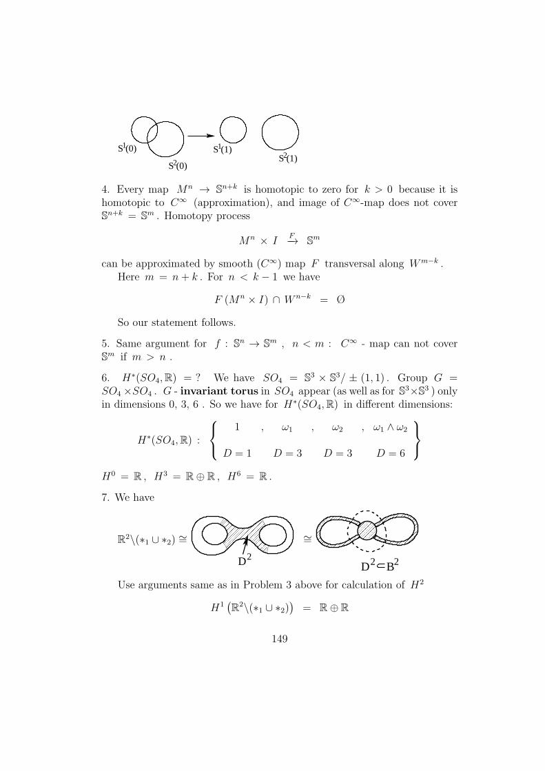
S (0)1 S (1)1
S (0)2 S (1)2
4. Every map Mn → Sn+k is homotopic to zero for k > 0 because it ishomotopic to C∞ (approximation), and image of C∞-map does not coverSn+k = Sm . Homotopy process
Mn × IF−→ Sm
can be approximated by smooth (C∞) map F transversal along Wm−k .Here m = n+ k . For n < k − 1 we have
F (Mn × I) ∩ W n−k = Ø
So our statement follows.
5. Same argument for f : Sn → Sm , n < m : C∞ - map can not coverSm if m > n .
6. H∗(SO4,R) = ? We have SO4 = S3 × S3/ ± (1, 1) . Group G =SO4 ×SO4 . G - invariant torus in SO4 appear (as well as for S3×S3 ) onlyin dimensions 0, 3, 6 . So we have for H∗(SO4,R) in different dimensions:
H∗(SO4,R) :
1 , ω1 , ω2 , ω1 ∧ ω2
D = 1 D = 3 D = 3 D = 6
H0 = R , H3 = R⊕ R , H6 = R .
7. We have
R2\(∗1 ∪ ∗2) ∼=
D2
∼=
D2 B2
Use arguments same as in Problem 3 above for calculation of H2
H1(R2\(∗1 ∪ ∗2)
)= R⊕ R
149
Lecture 32. Geodesics. Gauss Lemma.
1. Geodesics: smooth curves γ(t) = xi(t) such that
D
dt
dx
dt≡ 0 ( or ∇x x = 0 )
Equationxi + Γikj x
k xj = 0
Calculus of variation:
a) Length
l(γ) =
∫ b
a
|x(t)| dt =
∫ b
a
L0(x, x) dt
where
L0(x, x) =√gij(x) xi xj
is a “Lagrangian”.
b) “Action”
S(γ) =
∫ b
a
1
2gij(x) x
i xj dt =
∫ b
a
L1(x, x) dt
Euler - Lagrange equation (EL)
d
dt
∂L
∂xi=
∂L
∂xi
Momentum:
pi =∂L
∂xi
Energy:E = pi x
i − L
Conservation of energy:dE
dt≡ 0
For L = L1 we have
E = L1 =1
2gij(x) x
i xj =1
2∥x∥2
150
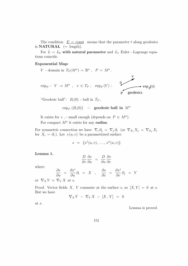
The condition E = const means that the parameter t along geodesicsis NATURAL (∼ length).
For L = L0 with natural parameter and L1 Euler - Lagrange equa-tions coincide.
Exponential Map:
V - domain in TP (Mn) = Rn , P = Mn .
expP : V → Mn , v ∈ TP , expP (V ) :0
v
P
exp (v)P
geodesics
“Geodesic ball”: Bϵ(0) - ball in TP ,
expP (Bϵ(0)) − geodesic ball in Mn
It exists for ϵ , - small enough (depends on P ∈ Mn).
For compact Mn it exists for any radius.
For symmetric connection we have ∇i ∂j = ∇j ∂i (or ∇XiXj = ∇Xj
Xi
for Xi = ∂i ). Let s (u, v) be a parametrized surface
s = x1(u, v), . . . , xn(u, v)
Lemma 1.D
∂v
∂s
∂u=
D
∂u
∂s
∂v
where∂s
∂u=
∂xi
∂u∂i = X ,
∂s
∂v=
∂xj
∂v∂j = Y
or ∇X Y = ∇Y X at s.
Proof. Vector fields X, Y commute at the surface s, so [X,Y ] = 0 at s.But we have
∇X Y − ∇Y X − [X , Y ] = 0
at s.Lemma is proved.
151
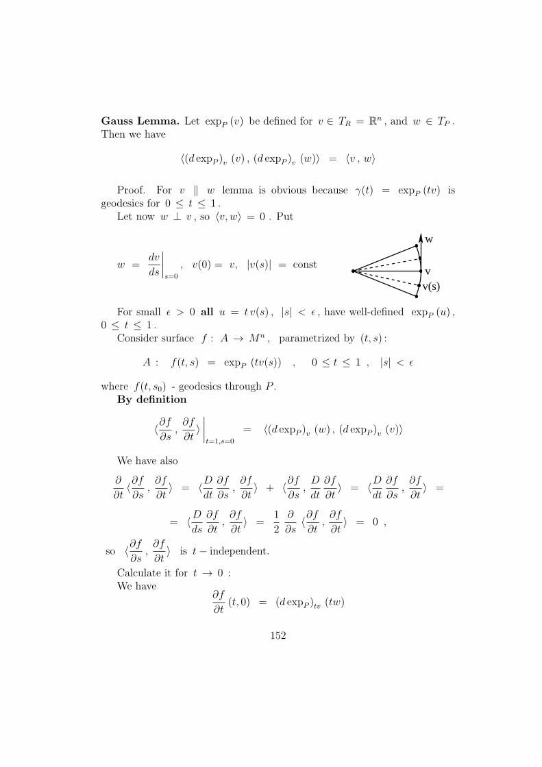
Gauss Lemma. Let expP (v) be defined for v ∈ TR = Rn , and w ∈ TP .Then we have
⟨(d expP )v (v) , (d expP )v (w)⟩ = ⟨v , w⟩
Proof. For v ∥ w lemma is obvious because γ(t) = expP (tv) isgeodesics for 0 ≤ t ≤ 1 .
Let now w ⊥ v , so ⟨v, w⟩ = 0 . Put
w =dv
ds
∣∣∣∣s=0
, v(0) = v, |v(s)| = const
v(s)v
w
For small ϵ > 0 all u = t v(s) , |s| < ϵ , have well-defined expP (u) ,0 ≤ t ≤ 1 .
Consider surface f : A → Mn , parametrized by (t, s) :
A : f(t, s) = expP (tv(s)) , 0 ≤ t ≤ 1 , |s| < ϵ
where f(t, s0) - geodesics through P .By definition
⟨∂f∂s
,∂f
∂t⟩∣∣∣∣t=1,s=0
= ⟨(d expP )v (w) , (d expP )v (v)⟩
We have also
∂
∂t⟨∂f∂s
,∂f
∂t⟩ = ⟨D
dt
∂f
∂s,∂f
∂t⟩ + ⟨∂f
∂s,D
dt
∂f
∂t⟩ = ⟨D
dt
∂f
∂s,∂f
∂t⟩ =
= ⟨Dds
∂f
∂t,∂f
∂t⟩ =
1
2
∂
∂s⟨∂f∂t
,∂f
∂t⟩ = 0 ,
so ⟨∂f∂s
,∂f
∂t⟩ is t− independent.
Calculate it for t → 0 :We have
∂f
∂t(t, 0) = (d expP )tv (tw)
152
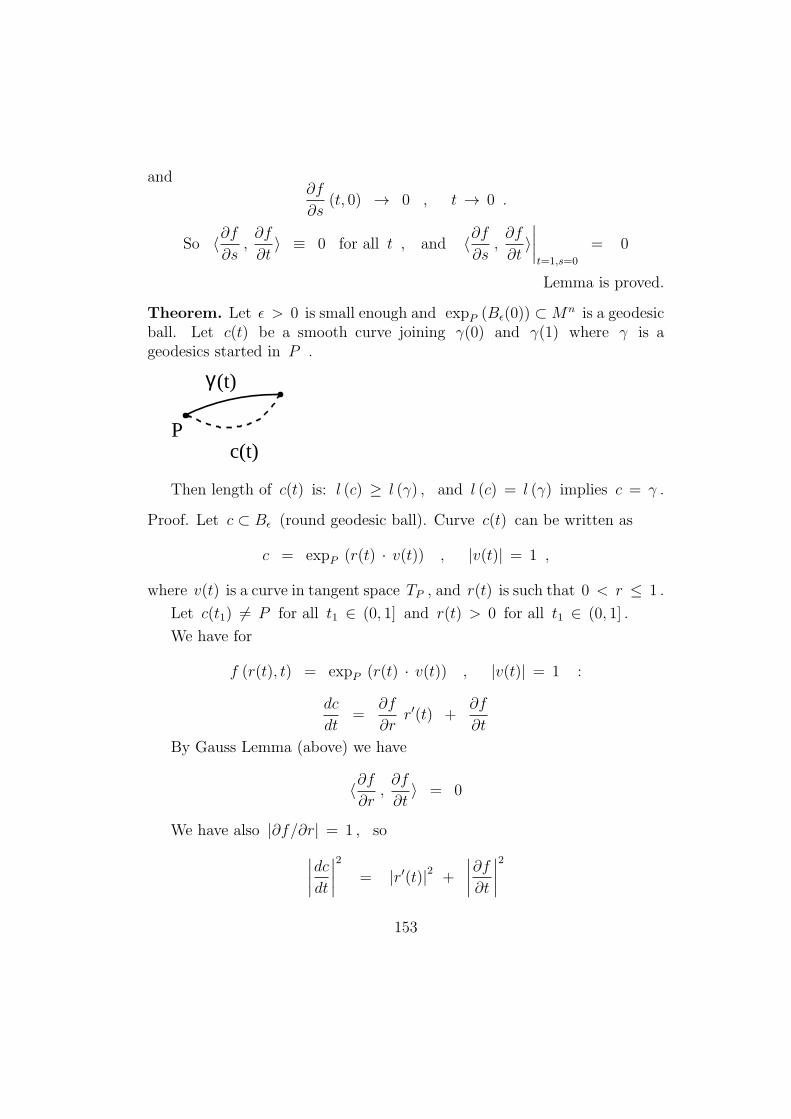
and∂f
∂s(t, 0) → 0 , t → 0 .
So ⟨∂f∂s
,∂f
∂t⟩ ≡ 0 for all t , and ⟨∂f
∂s,∂f
∂t⟩∣∣∣∣t=1,s=0
= 0
Lemma is proved.
Theorem. Let ϵ > 0 is small enough and expP (Bϵ(0)) ⊂Mn is a geodesicball. Let c(t) be a smooth curve joining γ(0) and γ(1) where γ is ageodesics started in P .
γ(t)
Pc(t)
Then length of c(t) is: l (c) ≥ l (γ) , and l (c) = l (γ) implies c = γ .
Proof. Let c ⊂ Bϵ (round geodesic ball). Curve c(t) can be written as
c = expP (r(t) · v(t)) , |v(t)| = 1 ,
where v(t) is a curve in tangent space TP , and r(t) is such that 0 < r ≤ 1 .
Let c(t1) = P for all t1 ∈ (0, 1] and r(t) > 0 for all t1 ∈ (0, 1] .
We have for
f (r(t), t) = expP (r(t) · v(t)) , |v(t)| = 1 :
dc
dt=
∂f
∂rr′(t) +
∂f
∂t
By Gauss Lemma (above) we have
⟨∂f∂r
,∂f
∂t⟩ = 0
We have also |∂f/∂r| = 1 , so∣∣∣∣dcdt∣∣∣∣2 = |r′(t)|2 +
∣∣∣∣∂f∂t∣∣∣∣2
153
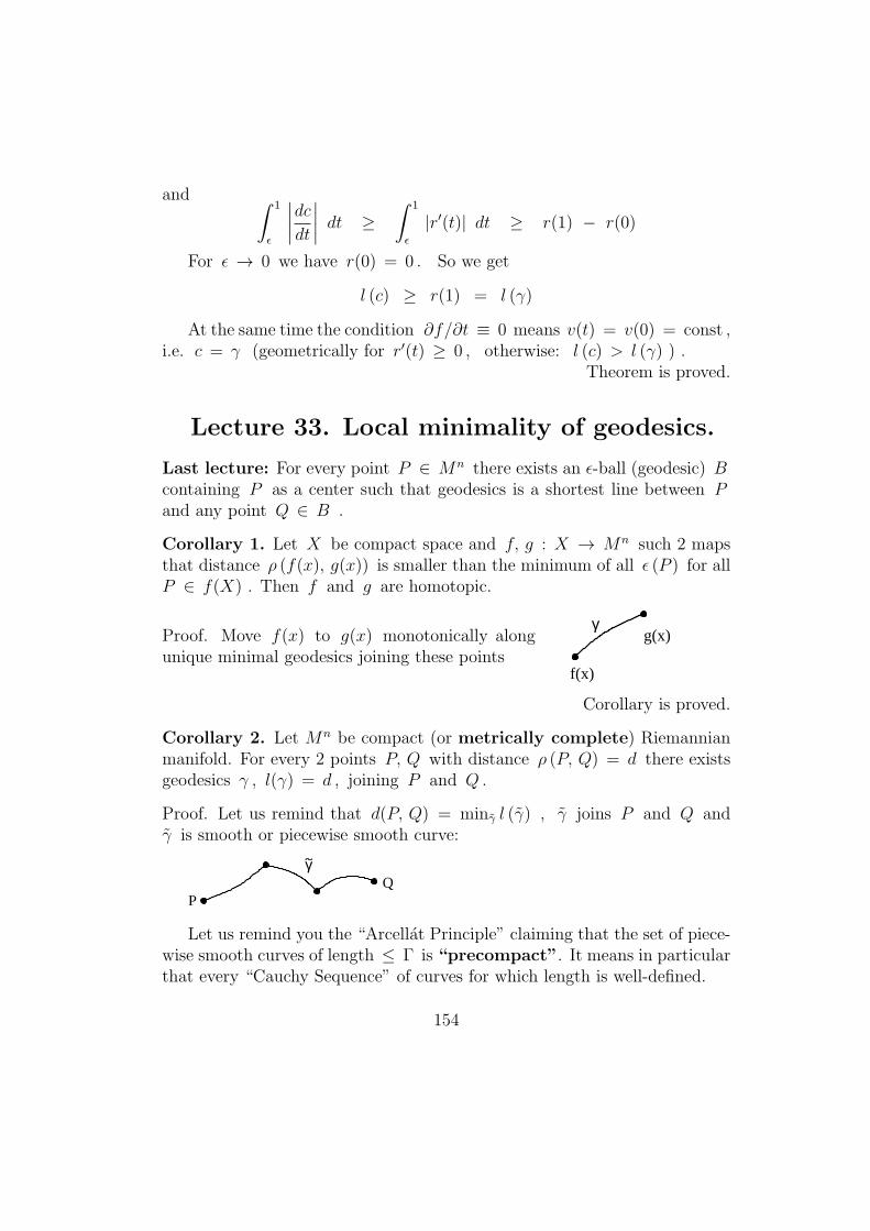
and ∫ 1
ϵ
∣∣∣∣dcdt∣∣∣∣ dt ≥
∫ 1
ϵ
|r′(t)| dt ≥ r(1) − r(0)
For ϵ → 0 we have r(0) = 0 . So we get
l (c) ≥ r(1) = l (γ)
At the same time the condition ∂f/∂t ≡ 0 means v(t) = v(0) = const ,i.e. c = γ (geometrically for r′(t) ≥ 0 , otherwise: l (c) > l (γ) ) .
Theorem is proved.
Lecture 33. Local minimality of geodesics.
Last lecture: For every point P ∈ Mn there exists an ϵ-ball (geodesic) Bcontaining P as a center such that geodesics is a shortest line between Pand any point Q ∈ B .
Corollary 1. Let X be compact space and f, g : X → Mn such 2 mapsthat distance ρ (f(x), g(x)) is smaller than the minimum of all ϵ (P ) for allP ∈ f(X) . Then f and g are homotopic.
Proof. Move f(x) to g(x) monotonically alongunique minimal geodesics joining these points
γ
f(x)
g(x)
Corollary is proved.
Corollary 2. Let Mn be compact (or metrically complete) Riemannianmanifold. For every 2 points P, Q with distance ρ (P, Q) = d there existsgeodesics γ , l(γ) = d , joining P and Q .
Proof. Let us remind that d(P, Q) = minγ l (γ) , γ joins P and Q andγ is smooth or piecewise smooth curve:
PQ
γ
Let us remind you the “Arcellat Principle” claiming that the set of piece-wise smooth curves of length ≤ Γ is “precompact”. It means in particularthat every “Cauchy Sequence” of curves for which length is well-defined.
154
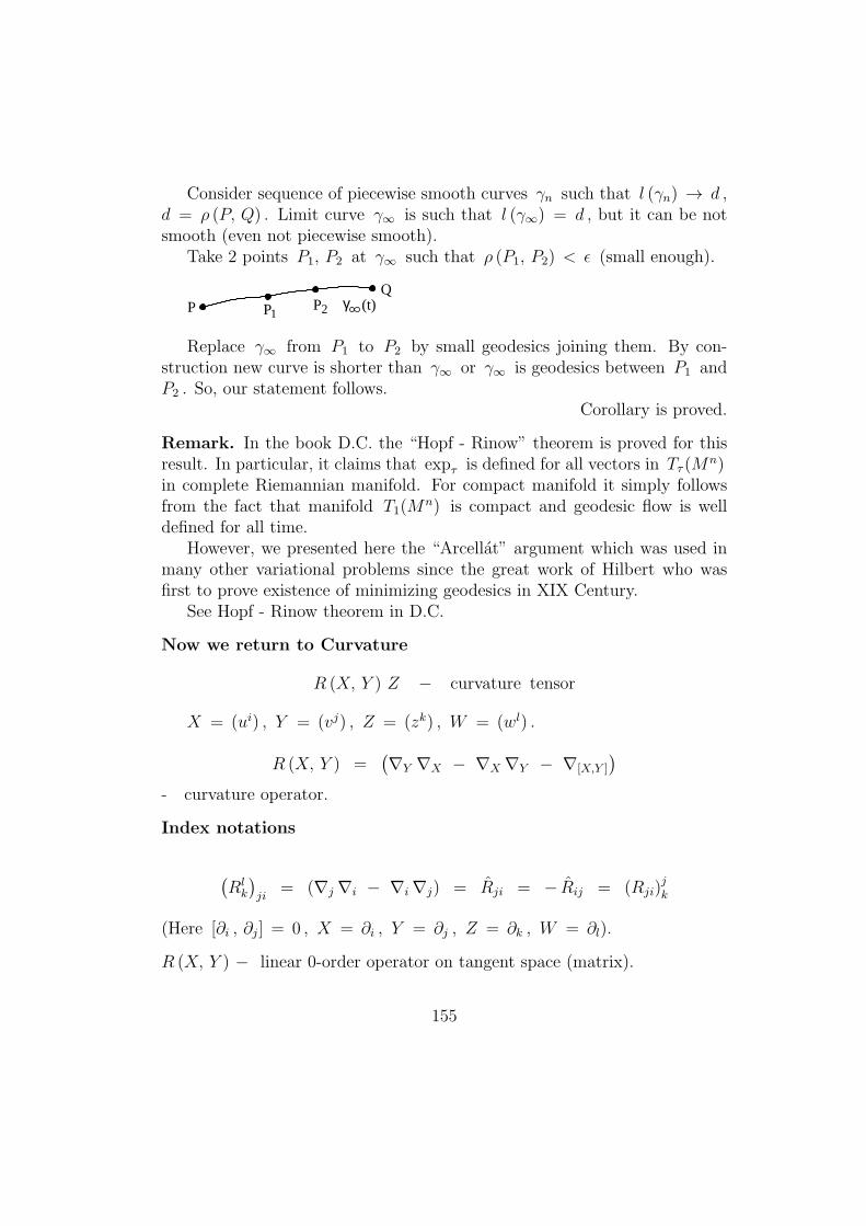
Consider sequence of piecewise smooth curves γn such that l (γn) → d ,d = ρ (P, Q) . Limit curve γ∞ is such that l (γ∞) = d , but it can be notsmooth (even not piecewise smooth).
Take 2 points P1, P2 at γ∞ such that ρ (P1, P2) < ϵ (small enough).
γ (t)P1P2P
Q
Replace γ∞ from P1 to P2 by small geodesics joining them. By con-struction new curve is shorter than γ∞ or γ∞ is geodesics between P1 andP2 . So, our statement follows.
Corollary is proved.
Remark. In the book D.C. the “Hopf - Rinow” theorem is proved for thisresult. In particular, it claims that expτ is defined for all vectors in Tτ (M
n)in complete Riemannian manifold. For compact manifold it simply followsfrom the fact that manifold T1(M
n) is compact and geodesic flow is welldefined for all time.
However, we presented here the “Arcellat” argument which was used inmany other variational problems since the great work of Hilbert who wasfirst to prove existence of minimizing geodesics in XIX Century.
See Hopf - Rinow theorem in D.C.
Now we return to Curvature
R (X, Y ) Z − curvature tensor
X = (ui) , Y = (vj) , Z = (zk) , W = (wl) .
R (X, Y ) =(∇Y ∇X − ∇X ∇Y − ∇[X,Y ]
)- curvature operator.
Index notations
(Rlk
)ji
= (∇j∇i − ∇i∇j) = Rji = − Rij = (Rji)jk
(Here [∂i , ∂j] = 0 , X = ∂i , Y = ∂j , Z = ∂k , W = ∂l).
R (X, Y ) − linear 0-order operator on tangent space (matrix).
155
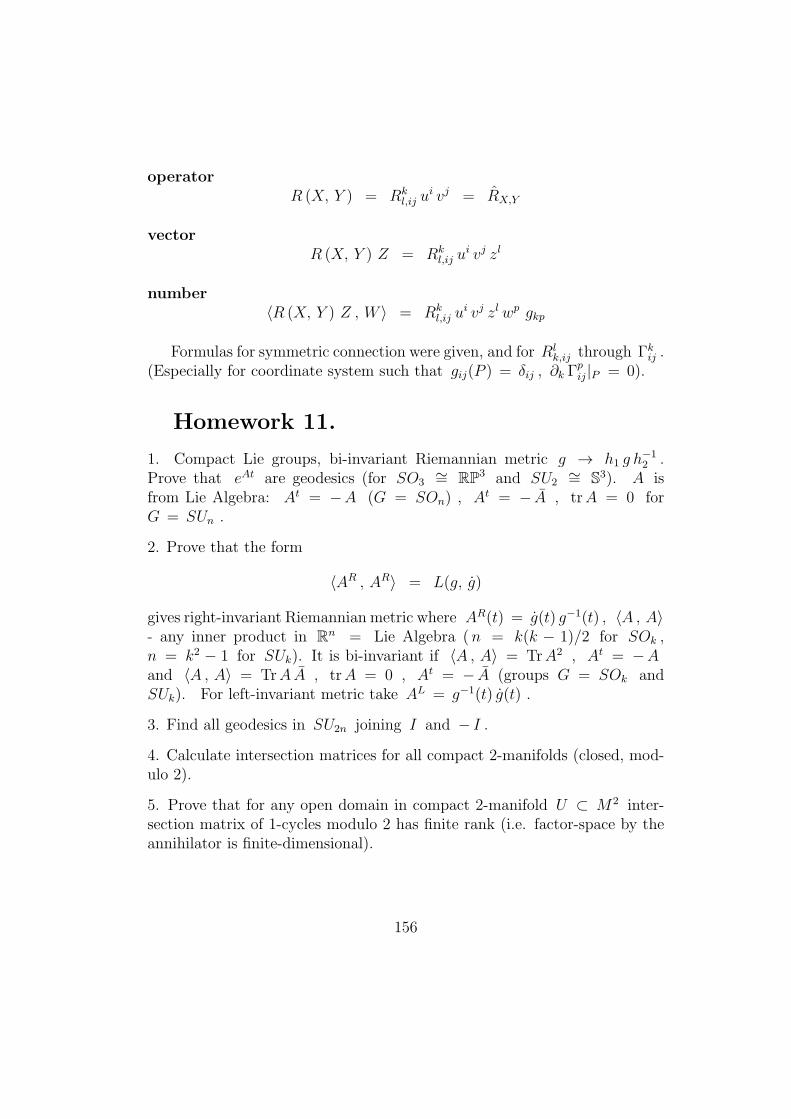
operatorR (X, Y ) = Rk
l,ij ui vj = RX,Y
vectorR (X, Y ) Z = Rk
l,ij ui vj zl
number⟨R (X, Y ) Z , W ⟩ = Rk
l,ij ui vj zl wp gkp
Formulas for symmetric connection were given, and for Rlk,ij through Γkij .
(Especially for coordinate system such that gij(P ) = δij , ∂k Γpij|P = 0).
Homework 11.
1. Compact Lie groups, bi-invariant Riemannian metric g → h1 g h−12 .
Prove that eAt are geodesics (for SO3∼= RP3 and SU2
∼= S3). A isfrom Lie Algebra: At = −A (G = SOn) , At = − A , trA = 0 forG = SUn .
2. Prove that the form
⟨AR , AR⟩ = L(g, g)
gives right-invariant Riemannian metric where AR(t) = g(t) g−1(t) , ⟨A , A⟩- any inner product in Rn = Lie Algebra (n = k(k − 1)/2 for SOk ,n = k2 − 1 for SUk). It is bi-invariant if ⟨A , A⟩ = TrA2 , At = −Aand ⟨A , A⟩ = TrA A , trA = 0 , At = − A (groups G = SOk andSUk). For left-invariant metric take AL = g−1(t) g(t) .
3. Find all geodesics in SU2n joining I and − I .
4. Calculate intersection matrices for all compact 2-manifolds (closed, mod-ulo 2).
5. Prove that for any open domain in compact 2-manifold U ⊂ M2 inter-section matrix of 1-cycles modulo 2 has finite rank (i.e. factor-space by theannihilator is finite-dimensional).
156
Lecture 34. Riemannian Curvature. Exam-
ples.
Consider Mn , ψ ∈ Rmx .
Curvature tensor.
Connection: ∇X , X = ∂i , ∇X ψ = ∂i ψ + Γi ψ
Curvature:∇X ∇Y − ∇Y ∇X − ∇[X,Y ] = R
X = ∂i , Y = ∂j , Rij = ∇i∇j − ∇j∇i : Rmx → Rm
x
1-form (locally) - connection
A = Γi dxi
2-form (locally) - curvature
R = Rij dxi ∧ dxj = dA + A ∧ A
(Matrix Multiplication).
R = dA +1
2[A ∧ A]
- same; written through the commutator - Lie Algebra multiplica-tion.
Gauge Transformation: ψ = G(x)φ(x)
Γi → G−1 ΓiG − G−1 ∂iG :
∇i (ψ) = ∇i (Gφ) = ∂i (Gφ) + Γi (Gφ)
or : G(∂i φ + G−1 ∂iG φ + G−1 ΓiG φ
)Rij → G−1 Rij G
(calculation).
Conclusion: for tangent bundle Rij = (Rlk,ij) is tensor.
157
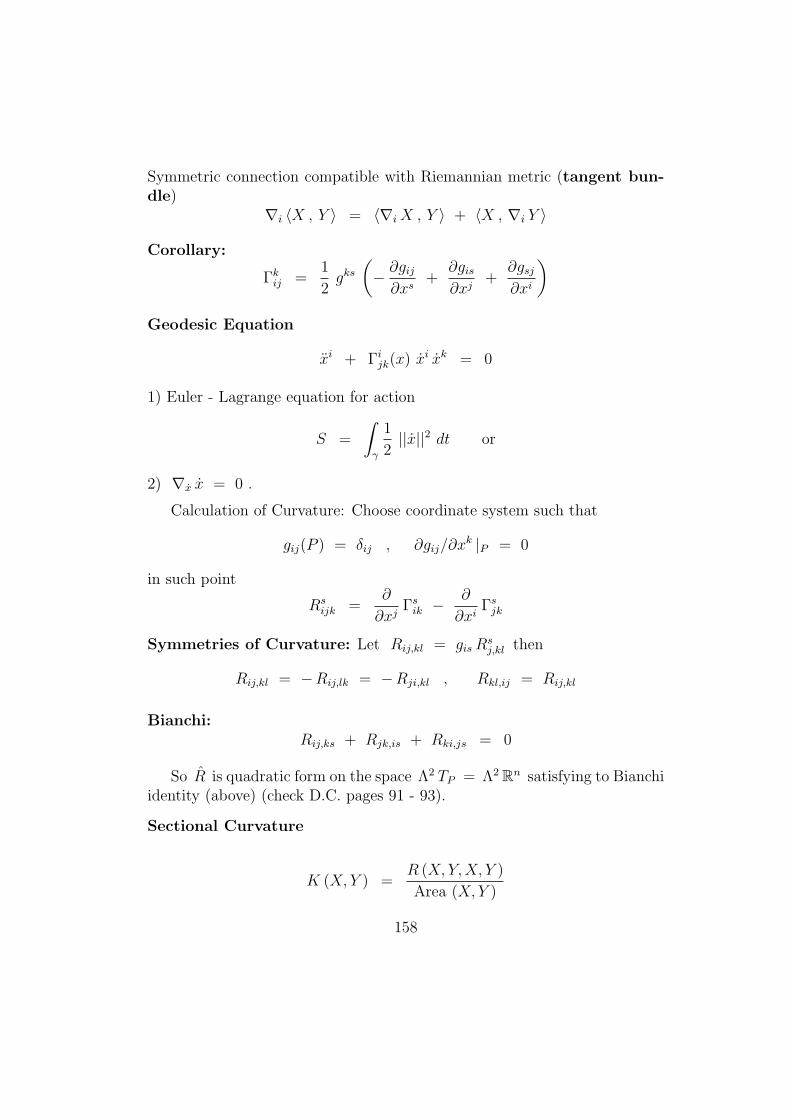
Symmetric connection compatible with Riemannian metric (tangent bun-dle)
∇i ⟨X , Y ⟩ = ⟨∇iX , Y ⟩ + ⟨X , ∇i Y ⟩
Corollary:
Γkij =1
2gks
(− ∂gij∂xs
+∂gis∂xj
+∂gsj∂xi
)Geodesic Equation
xi + Γijk(x) xi xk = 0
1) Euler - Lagrange equation for action
S =
∫γ
1
2||x||2 dt or
2) ∇x x = 0 .
Calculation of Curvature: Choose coordinate system such that
gij(P ) = δij , ∂gij/∂xk |P = 0
in such point
Rsijk =
∂
∂xjΓsik −
∂
∂xiΓsjk
Symmetries of Curvature: Let Rij,kl = gisRsj,kl then
Rij,kl = −Rij,lk = −Rji,kl , Rkl,ij = Rij,kl
Bianchi:Rij,ks + Rjk,is + Rki,js = 0
So R is quadratic form on the space Λ2 TP = Λ2Rn satisfying to Bianchiidentity (above) (check D.C. pages 91 - 93).
Sectional Curvature
K (X, Y ) =R (X, Y,X, Y )
Area (X,Y )
158
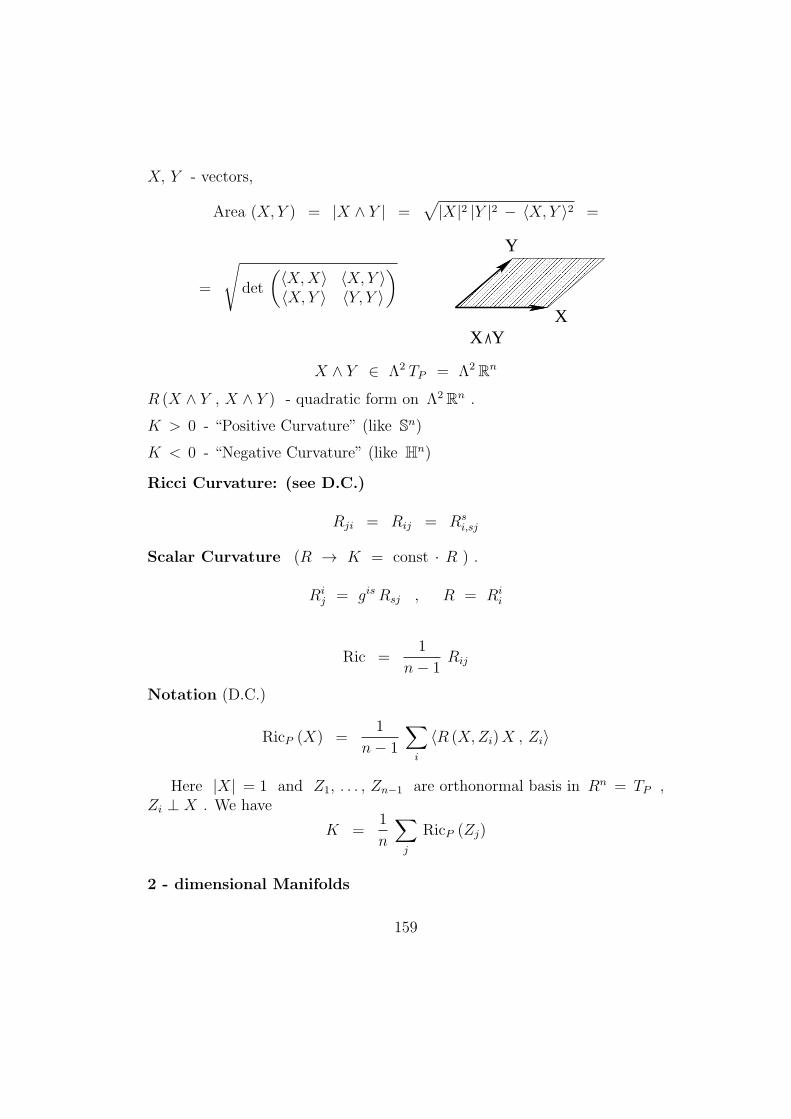
X, Y - vectors,
Area (X, Y ) = |X ∧ Y | =√|X|2 |Y |2 − ⟨X, Y ⟩2 =
=
√det
(⟨X,X⟩ ⟨X,Y ⟩⟨X, Y ⟩ ⟨Y, Y ⟩
)
X
Y
X Y
X ∧ Y ∈ Λ2 TP = Λ2 Rn
R (X ∧ Y , X ∧ Y ) - quadratic form on Λ2 Rn .
K > 0 - “Positive Curvature” (like Sn)
K < 0 - “Negative Curvature” (like Hn)
Ricci Curvature: (see D.C.)
Rji = Rij = Rsi,sj
Scalar Curvature (R → K = const · R ) .
Rij = gisRsj , R = Ri
i
Ric =1
n− 1Rij
Notation (D.C.)
RicP (X) =1
n− 1
∑i
⟨R (X,Zi)X , Zi⟩
Here |X| = 1 and Z1, . . . , Zn−1 are orthonormal basis in Rn = TP ,Zi ⊥ X . We have
K =1
n
∑j
RicP (Zj)
2 - dimensional Manifolds
159
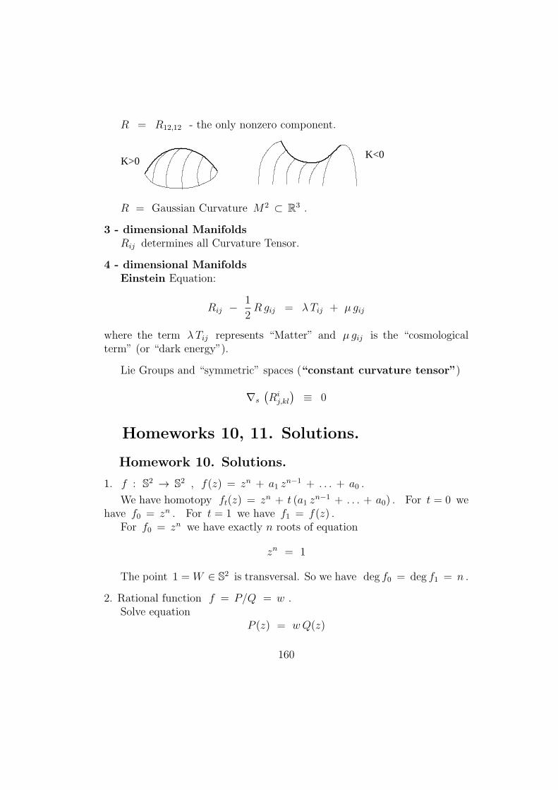
R = R12,12 - the only nonzero component.
K>0K<0
R = Gaussian Curvature M2 ⊂ R3 .
3 - dimensional ManifoldsRij determines all Curvature Tensor.
4 - dimensional ManifoldsEinstein Equation:
Rij −1
2Rgij = λTij + µ gij
where the term λTij represents “Matter” and µ gij is the “cosmologicalterm” (or “dark energy”).
Lie Groups and “symmetric” spaces (“constant curvature tensor”)
∇s
(Rij,kl
)≡ 0
Homeworks 10, 11. Solutions.
Homework 10. Solutions.
1. f : S2 → S2 , f(z) = zn + a1 zn−1 + . . . + a0 .
We have homotopy ft(z) = zn + t (a1 zn−1 + . . . + a0) . For t = 0 we
have f0 = zn . For t = 1 we have f1 = f(z) .For f0 = zn we have exactly n roots of equation
zn = 1
The point 1 = W ∈ S2 is transversal. So we have deg f0 = deg f1 = n .
2. Rational function f = P/Q = w .Solve equation
P (z) = wQ(z)
160
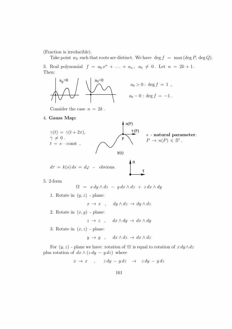
(Fraction is irreducible).Take point w0 such that roots are distinct. We have deg f = max (degP, degQ).
3. Real polynomial f = a0 xn + . . . + an , a0 = 0 . Let n = 2k + 1 .
Then:
a <0a >00 0a0 > 0 : deg f = 1 ,
a0 − 0 : deg f = −1 .
Consider the case n = 2k .
4. Gauss Map:
γ(t) = γ(t+ 2π),γ = 0 .t = s · const ,
γ(t)
(P)τ
n(P)
Ps - natural parameter.P → n(P ) ∈ S1 .
dτ = k(s) ds = dφ - obvious.τ
n
5. 2-formΩ = x dy ∧ dz − y dx ∧ dz + z dx ∧ dy
1. Rotate in (y, z) - plane:
x → x , dy ∧ dz → dy ∧ dz
2. Rotate in (x, y) - plane:
z → z , dx ∧ dy → dx ∧ dy
3. Rotate in (x, z) - plane:
y → y , dx ∧ dz → dx ∧ dz
For (y, z) - plane we have: rotation of Ω is equal to rotation of x dy∧dzplus rotation of dx ∧ (z dy − y dz) where
x → x , z dy − y dz → z dy − y dz
161
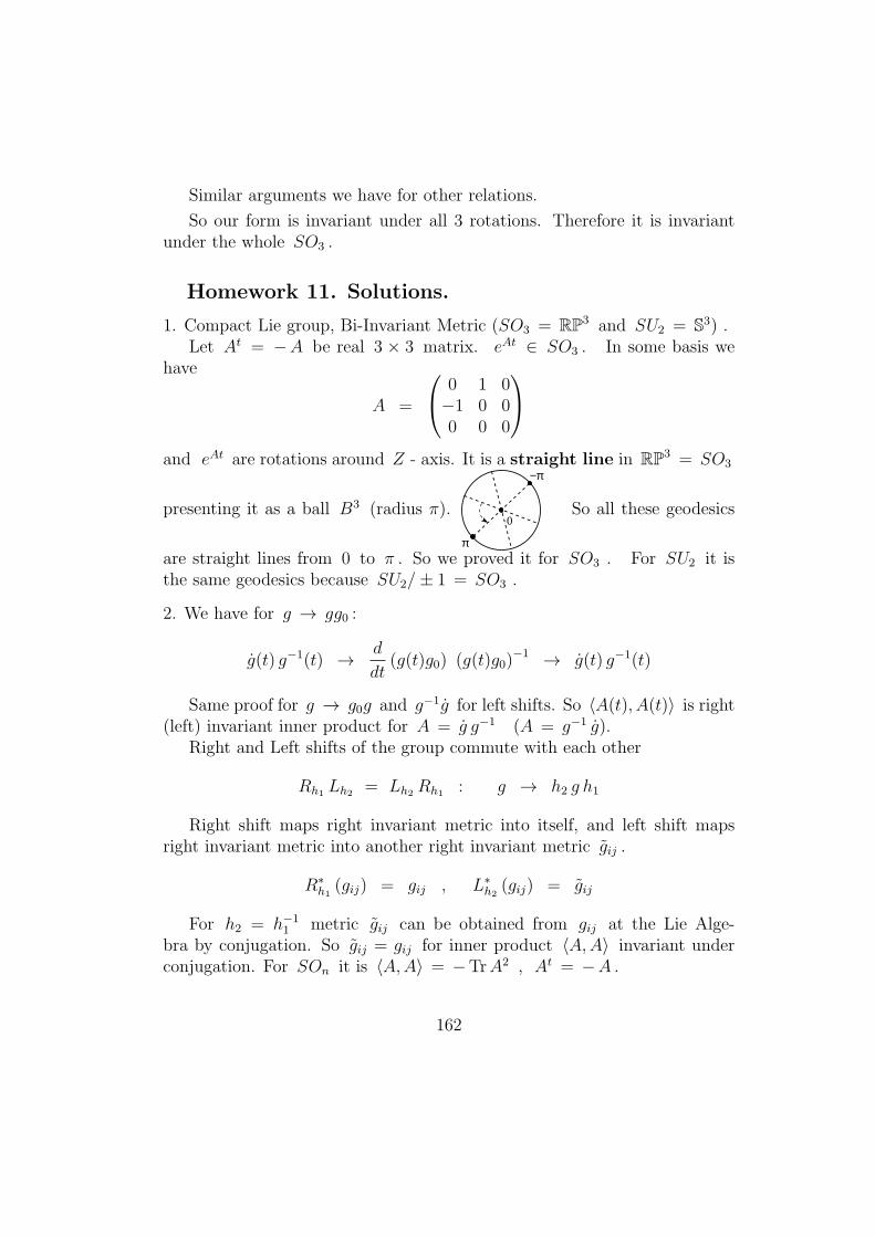
Similar arguments we have for other relations.
So our form is invariant under all 3 rotations. Therefore it is invariantunder the whole SO3 .
Homework 11. Solutions.
1. Compact Lie group, Bi-Invariant Metric (SO3 = RP3 and SU2 = S3) .Let At = −A be real 3 × 3 matrix. eAt ∈ SO3 . In some basis we
have
A =
0 1 0−1 0 00 0 0
and eAt are rotations around Z - axis. It is a straight line in RP3 = SO3
presenting it as a ball B3 (radius π).0
−π
π
So all these geodesics
are straight lines from 0 to π . So we proved it for SO3 . For SU2 it isthe same geodesics because SU2/± 1 = SO3 .
2. We have for g → gg0 :
g(t) g−1(t) → d
dt(g(t)g0) (g(t)g0)
−1 → g(t) g−1(t)
Same proof for g → g0g and g−1g for left shifts. So ⟨A(t), A(t)⟩ is right(left) invariant inner product for A = g g−1 (A = g−1 g).
Right and Left shifts of the group commute with each other
Rh1 Lh2 = Lh2 Rh1 : g → h2 g h1
Right shift maps right invariant metric into itself, and left shift mapsright invariant metric into another right invariant metric gij .
R∗h1(gij) = gij , L∗
h2(gij) = gij
For h2 = h−11 metric gij can be obtained from gij at the Lie Alge-
bra by conjugation. So gij = gij for inner product ⟨A,A⟩ invariant underconjugation. For SOn it is ⟨A,A⟩ = −TrA2 , At = −A .
162
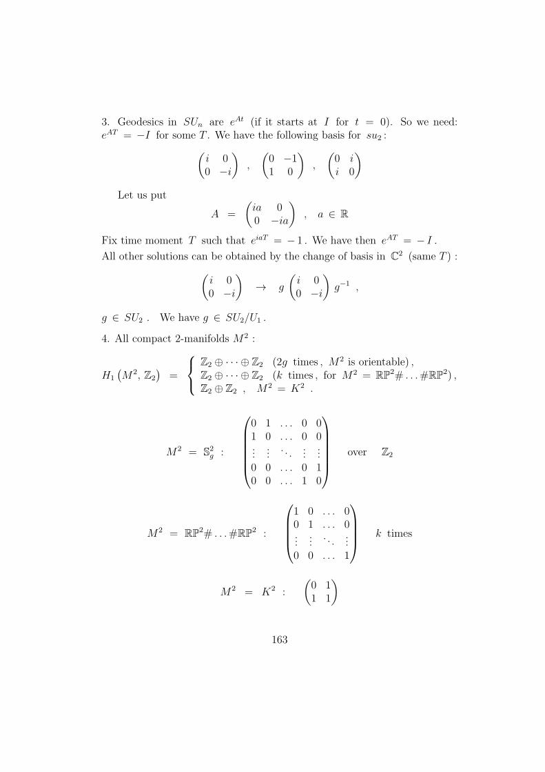
3. Geodesics in SUn are eAt (if it starts at I for t = 0). So we need:eAT = −I for some T . We have the following basis for su2 :(
i 00 −i
),
(0 −11 0
),
(0 ii 0
)Let us put
A =
(ia 00 −ia
), a ∈ R
Fix time moment T such that eiaT = − 1 . We have then eAT = − I .All other solutions can be obtained by the change of basis in C2 (same T ) :(
i 00 −i
)→ g
(i 00 −i
)g−1 ,
g ∈ SU2 . We have g ∈ SU2/U1 .
4. All compact 2-manifolds M2 :
H1
(M2, Z2
)=
Z2 ⊕ · · · ⊕ Z2 (2g times , M2 is orientable) ,Z2 ⊕ · · · ⊕ Z2 (k times , for M2 = RP2# . . .#RP2) ,Z2 ⊕ Z2 , M2 = K2 .
M2 = S2g :
0 1 . . . 0 01 0 . . . 0 0...
.... . .
......
0 0 . . . 0 10 0 . . . 1 0
over Z2
M2 = RP2# . . .#RP2 :
1 0 . . . 00 1 . . . 0...
.... . .
...0 0 . . . 1
k times
M2 = K2 :
(0 11 1
)
163
K2#RP2 = T2 #RP2 = RP2 #RP2 #RP2 (?)
K2 = RP2 #RP2 (?)
5. Let U be an open domain in any compact 2-manifold M2 . Then inter-section matrix
H1 (U, Z2) → H1
(M2, Z2
)depends only on image of cycles in M2 where it has finite rank. So innerproduct in H1 (U, Z2) also has finite rank.
164