Basic Books in Science

Book 2

Space:From Euclid to Einstein

Roy McWeeny

Basic Books in Science

– a Series of books that start at the beginning

Book 2

Space – from Euclid to Einstein

Roy McWeeny

Professore Emerito di Chimica Teorica, Universita di Pisa, Pisa

(Italy)

The Series is maintained, with regular updating and improvement,

at

http://www.learndev.org/ScienceWorkBooks.html

and the books may be downloaded entirely free of charge.

This book is licensed under a Creative Commons

Attribution-ShareAlike 3.0 Unported License.

(Last updated 24 September 2011)

BASIC BOOKS IN SCIENCE

About this Series

All human progress depends on education: to get it we need books and schools. ScienceEducation is of key importance.

Unfortunately, books and schools are not always easy to find. But nowadays all the world’sknowledge should be freely available to everyone – through the Internet that connects allthe world’s computers.

The aim of the Series is to bring basic knowledge in all areas of science within the reachof everyone. Every Book will cover in some depth a clearly defined area, starting from thevery beginning and leading up to university level, and will be available on the Internet atno cost to the reader. To obtain a copy it should be enough to make a single visit to anylibrary or public office with a personal computer and a telephone line. Each book willserve as one of the ‘building blocks’ out of which Science is built; and together they willform a ‘give-away’ science library.

About this book

This book, like the others in the Series, is written in simple English – the language mostwidely used in science and technology. It takes the next big step beyond “Number andsymbols” (the subject of Book 1), starting from our first ideas about the measurementof distance and the relationships among objects in space. It goes back to the work ofthe philosophers and astronomers of two thousand years ago; and it extends to that ofEinstein, whose work laid the foundations for our present-day ideas about the nature ofspace itself. This is only a small book; and it doesn’t follow the historical route, startingfrom geometry the way Euclid did it (as we learnt it in our schooldays); but it aims to givean easier and quicker way of getting to the higher levels needed in Physics and relatedsciences.

ii

Looking ahead –Like the first book in the Series, Book 2 spans more than two thousand years of discovery.It is about the science of space – geometry – starting with the Greek philosophers,Euclid and many others, and leading to the present – when space and space travel iswritten about even in the newspapers and almost everyone has heard of Einstein and hisdiscoveries.

Euclid and his school didn’t trust the use of numbers in geometry (you saw why in Book1): they used pictures instead. But now you’ve learnt things they didn’t know about –and will find you can go further, and faster, by using numbers and algebra. And again,you’ll pass many ‘milestones’:

• In Chapter 1 you start from distance, expressed as a number of units, and seehow Euclid’s ideas about straight lines, angles and triangles can be ‘translated’ intostatements about distances and numbers.

• Most of Euclid’s work was on geometry of the plane; but in Chapter 2 you’llsee how any point in a plane is fixed by giving two numbers and how lines can bedescribed by equations.

• The ideas of area and angle come straight out of plane geometry (in Chapter3): you find how to get the area of a circle and how to measure angles.

• Chapter 4 is hard, because it ties together so many very different ideas, mostlyfrom Book 1 – operators, vectors, rotations, exponentials, and complexnumbers – they are all connected!

• Points which are not all in the same plane, lie in 3-dimensional space – youneed three numbers to say where each one is. In Chapter 5 you’ll find the geometryof 3-space is just like that of 2-space; but it looks easier if you use vectors.

• Plane shapes, such as triangles, have properties like area, angle and side-lengthsthat don’t change if you move them around in space: they belong to the shape itselfand are called invariants. Euclid used such ideas all the time. Now you’ll go from2-space to 3-space, where objects also have volume; and you can still do everythingwithout the pictures.

• After two thousand years people reached the last big milestone (Chapter 7): theyfound that Euclid’s geometry was very nearly, but not quite, perfect. And you’llwant to know how Einstein changed our ideas.

iii

CONTENTS

Chapter 1 Euclidean space

1.1 Distance

1.2 Foundations of Euclidean geometry

Chapter 2 Two-dimensional space

2.1 Parallel straight lines. Rectangles

2.2 Points and straight lines in 2-space

2.3 When and where will two straight lines meet?

Chapter 3 Area and angle

3.1 What is area?

3.2 How to measure angles

3.3 More on Euclid

Chapter 4 Rotations: bits and pieces

Chapter 5 Three-dimensional space

5.1 Planes and boxes in 3-space – coordinates

5.2 Describing simple objects in 3-space

5.3 Using vectors in 3-space

5.4 Scalar and vector products

5.5 Some examples

Chapter 6 Area and volume: invariance

6.1 Invariance of lengths and angles

6.2 Area and volume

6.3 Area in vector form

6.4 Volume in vector form

Chapter 7 Some other kinds of space

7.1 Many-dimensional space

7.2 Space-time and Relativity

7.3 Curved spaces: General Relativity

Notes to the Reader. When Chapters have several Sections they are numbered sothat “Section 2.3” will mean “Chapter 2, Section 3”. Similarly, “equation (2.3)” willmean “Chapter 2, equation 3”. Important ‘key’ words are printed in boldface: they arecollected in the Index at the end of the book, along with the numbers of the pages whereyou can find them.

iv

Chapter 1

Euclidean space

1.1 Distance

At the very beginning of Book 1 we talked about measuring the distance from home toschool by counting how many strides, or paces, it took to get there: the pace was the unitof distance and the number of paces was the measure of that particular distance. Nowwe want to make the idea more precise.

The standard unit of distance is ‘1 metre’ (or 1 m, for short) and is defined in a ‘measuring-rod’, with marks at its two ends, the distance between them fixing the unit. Any otherpair of marks (e.g. on some other rod, or stick) are also 1 m apart if they can be put incontact, at the same time, with those on the standard rod; and in this way we can makeas many copies of the unit as we like, all having the same length. In Book 1 we measureddistances by putting such copies end-to-end (the ‘law of combination’ for distances) andif, say, three such copies just reached from one point to another then the two points were‘3 m apart’ – the ‘distance between them was 3 m’, or ‘the length of the path from oneto the other was 3 m’ (three different ways of saying the same thing!).

Now the number of units needed to reach from one point ‘A’ to another point ‘B’ willdepend on how they are put together: if they form a ‘wiggly’ line, like a snake, you willneed more of them – the path will be longer. But the distance does not change: it is theunique (one and one only) shortest path length leading from A to B. (Of course the pathlength may not be exactly a whole number of units, but by setting up smaller and smaller‘mini-units’ – as in Book 1, Chapter 4 – it can be measured as accurately as we pleaseand represented by a decimal number.) The important thing is that the distance AB isthe length of the shortest path between A and B. In practice, this can be obtained bymarking the units (and mini-units) on a string, or tape, instead of a stiff measuring-rod:when the tape measure is pulled tight it can give a fairly accurate measure of the distanceAB. The shortest path defines a straight line between the points A and B.

One thing we must remember about measuring distance (or any other quantity, like massor time) – it’s always a certain number of units, not the number itself. The distance fromhome to school may be 2000 m (the unit being the metre), but 2000 by itself is just anumber: quantity = number × unit, where the number is the measure of the quantity

1

in terms of a chosen unit. We can always change the unit: if a distance is large we canmeasure it in kilometres (km) and since 1 km means 1000 m the distance (d, say) fromhome to school will be d = 2000 m = 2 km. If we make the unit a thousand times bigger,the number that measures a certain quantity will become a thousand times smaller. Thus,

d = old measure× old unit= new measure× new unit= old measure

1000× (1000× old unit)

and the same rule always holds. In some countries the unit of distance is the ‘mile’ andthere are roughly 8 km to every 5 miles: 1 mile = (8/5) km. Thus, if I want a distance inmiles instead of kilometers, (new unit)= (8/5)×(old unit) and (new measure)=(5/8)×(oldmeasure). In this way we see the distance to the school is (5/8)×2 mile = 1.25 mile.Doing calculations with quantities is often called ‘quantity calculus’ – but there’s nothingmysterious about it, it’s just ‘common sense’ !

Euclidean geometry (the science of space) is based on the foundations laid by Euclid,the Greek philosopher, working around 300 BC) it starts from the concepts of points andstraight lines; and it still gives a good description of the spatial relationships we deal within everyday life. But more than 2000 years later Einstein showed that, in dealing with vastdistances and objects travelling at enormous speeds, Euclidean geometry does not quitefit the experimental facts: the theory of relativity was born. One of the fundamentaldifferences, in going from Euclid to Einstein, is that the shortest path between two pointsis not quite a ‘straight line’ – that space is ‘curved’. There is nothing strange about this:a ship does not follow the shortest path between two points on the surface of the earth– because the earth is like a big ball, the surface is not flat, and what seems to be theshortest path (according to the compass) is in reality not a straight line but a curve. Thestrange thing is that space itself is very slightly ‘bent’, especially near very heavy thingslike the sun and the stars, so that Euclid’s ideas are never perfectly correct – they aresimply so close to the truth that, in everyday life, we can accept them without worrying.

In nearly all of Book 2 we’ll be talking about Euclidean geometry. But instead of doingit as Euclid did – and as it’s done even today in many schools all over the world – we’llmake use of algebra (Book 1) from the start. So we won’t follow history. Remember, theGreeks would not accept irrational numbers (Book 1, Chapter 4) so they couldn’t expresstheir ideas about space in terms of distances and had to base their arguments entirelyon pictures, not on numbers. This was why algebra and geometry grew up separately,for two thousand years. By looking at mathematics as a whole (not as a subject withmany branches, such as algebra, geometry, trigonometry) we can reach our goal muchmore easily.

1.2 Foundations of Euclidean geometry

The fact that the space we live in has a ‘distance property’ – that we can experimentallymeasure the distance between any two points, A and B say, and give it a number – will

2

be our starting point. We make it into an ‘axiom’ (one of the basic principles, which wetake as ‘given’):

The distance axiom

There is a unique (one and one only) shortest path between two points, Aand B, called the straight line AB; its length is the distance between A andB.

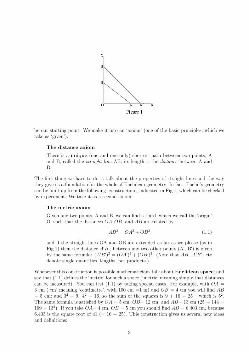
The first thing we have to do is talk about the properties of straight lines and the waythey give us a foundation for the whole of Euclidean geometry. In fact, Euclid’s geometrycan be built up from the following ‘construction’, indicated in Fig.1, which can be checkedby experiment. We take it as a second axiom:

The metric axiom

Given any two points, A and B, we can find a third, which we call the ‘origin’O, such that the distances OA,OB, and AB are related by

AB2 = OA2 + OB2 (1.1)

and if the straight lines OA and OB are extended as far as we please (as inFig.1) then the distance A′B′, between any two other points (A′, B′) is givenby the same formula: (A′B′)2 = (OA′)2 + (OB′)2. (Note that AB, A′B′, etcdenote single quantities, lengths, not products.)

Whenever this construction is possible mathematicians talk about Euclidean space; andsay that (1.1) defines the ‘metric’ for such a space (‘metric’ meaning simply that distancescan be measured). You can test (1.1) by taking special cases. For example, with OA =3 cm (‘cm’ meaning ‘centimetre’, with 100 cm =1 m) and OB = 4 cm you will find AB= 5 cm; and 32 = 9, 42 = 16, so the sum of the squares is 9 + 16 = 25 – which is 52.The same formula is satisfied by OA = 5 cm, OB= 12 cm, and AB= 13 cm (25 + 144 =169 = 132). If you take OA= 4 cm, OB = 5 cm you should find AB = 6.403 cm, because6.403 is the square root of 41 (= 16 + 25). This construction gives us several new ideasand definitions:

3

• The lines OA and OB in Fig.1 are perpendicular or at right angles. The straightlines formed by moving A and B further and further away from the origin O, in eitherdirection, are called axes. OX is the x-axis, OY is the y-axis.

• The points O, A, and B, define a ‘right-angled’ triangle, OAB, with the straightlines OA,OB,AB as its three sides. (The ‘tri’ means three and the ‘angle’ refers tothe lines OA and OB and will measure how much we must turn one line around theorigin O to make it point the same way as the other line – more about this later!)

• All straight lines, such as AB or A′B′, which intersect (i.e. cross at a single point)both axes, are said to ‘lie in a plane’ defined by the two axes.

From the axiom (1.1) and the definitions which follow it, the whole of geometry – thescience we need in making maps, in dividing out the land, in designing buildings, andeverything else connected with relationships in space – can be built up. Euclid startedfrom different axioms and argued with pictures, obtaining key results called theoremsand other results (called corollaries) that follow directly from them. He proved thetheorems one by one, in a logical order where each depends on theorems already proved.He published them in the 13 books of his famous work called “The Elements”, which setthe pattern for the teaching of geometry throughout past centuries. Here we use insteadthe methods of algebra (Book 1) and find that the same chain of theorems can be provedmore easily. Of course we won’t try to do the whole of geometry; but we’ll look at thefirst few links in the chain – finding that we don’t need to argue with pictures, we cando it all with numbers! The pictures are useful because they remind us of what we aredoing; but our arguments will be based on distances and these are measured by numbers.

This way of doing things is often called analytical geometry, but it’s better not to thinkof it as something separate from the rest – it’s just a part of a ‘unified’ (‘made-into-one’)mathematics.

Exercises

(1) Make a tape measure from a long piece of tape or string, using a metre rule to markthe centimetres, and use it to measure

• the distance (d) between opposite corners of this page of your book;

• the lengths of the different sides (x and y);

• the distance (AB) between two points (A and B) on the curved surface of a bigdrum (like the ones used for holding water), keeping the tape tightly stretched andalways at the same height;

• the distance between A and B (call it L), when A and B come close together andthe tape goes all the way round (this is called the circumference of the drum);

• the distance between two opposite points on the bottom edge of the drum (this –call it D – is the diameter of the drum).

4

(2) Check that the sum of x2 and y2 gives you d2, as (1.1) says it should.

(3) Note that L is several times bigger than D: how many? (Your answer should give youroughly the number π (called “pi”) that gave the Greeks so much trouble – as we knowfrom Book 1)

(4) In some countries small distances are measured in “inches” instead of cm, 1 inchbeing roughly 2.5 cm (the length of the last bit of your thumb). Put into inches all thedistances you measured in Exercise 1. Show that the answers you got in Exercises 2 and3 are unchanged.

(5) Make a simple set square – a triangle like OAB in Fig.1, with sides of 9 cm, 12 cmand 15 cm, cut out from a piece of stiff card. Use it to mark out axes OX and OY ona big sheet of paper (e.g. newspaper or wrapping paper). Then choose several pairs ofpoints, like A,B or A′,B′ in Fig.1, and verify that the distances AB,A′B′ etc. are alwaysrelated to OA and OB (or OA′ and OB′ etc.) by equation (1.1).

(6) Take a big rectangular box and measure the lengths (a, b, c) of the three differentedges and the distance (d) between opposite corners (the ones as far apart as you canget). Show, from your measurements, that d2 ≈ a2 + b2 + c2, where the sign ≈ means‘approximately’ or ‘nearly’ equal. Use the formula (1.1) to show that the ‘exact’ resultshould be

d2 = a2 + b2 + c2.

(Measurements are never quite perfect – so you can never use them to prove something.)

5

Chapter 2

Two-dimensional space

2.1 Parallel straight lines.

Rectangles

A plane has been defined in the last Section: it is a region based on two intersectingstraight lines of unlimited length, called axes. All straight lines which cut the two axeslie in the same plane and any pair with one point in common (to take as ‘origin’) can beused as alternative axes. Such a plane is a two-dimensional region called, for short, a2-space.

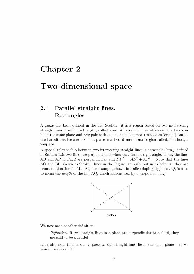
A special relationship between two intersecting straight lines is perpendicularity, definedin Section 1.2: two lines are perpendicular when they form a right angle. Thus, the linesAB and AP in Fig.2 are perpendicular and BP 2 = AB2 + AP 2. (Note that the linesAQ and BP, shown as ‘broken’ lines in the Figure, are only put in to help us: they are“construction lines”. Also AQ, for example, shown in Italic (sloping) type as AQ, is usedto mean the length of the line AQ, which is measured by a single number.)

We now need another definition:

Definition. If two straight lines in a plane are perpendicular to a third, theyare said to be parallel.

Let’s also note that in our 2-space all our straight lines lie in the same plane – so wewon’t always say it!

6

With this definition we can go to a first theorem:

Theorem. Any straight line perpendicular to one of two parallel straight linesis also perpendicular to the other.

Proof (If you find a proof hard, skip it; you can come back to it any time.)

Suppose AB and PQ in Fig.2 are parallel, both being perpendicular to AP (as in theDefinition), and that BQ is the other straight line perpendicular to AB. Then we mustshow that BQ is also perpendicular to PQ. In symbols, using (1.1),

Given AP 2 + PQ2 = AQ2,

show that BQ2 + QP 2 = BP 2 = BA2 + AP 2.

We must show that there is a point Q such that these relationships hold.

The lengths BQ and QP are unknown (they depend on where we put Q), but the possi-bilities are

(a) BQ = AP, PQ = AB,(b) BQ = AP, PQ 6= AB,(c) BQ 6= AP, PQ = AB,(d) BQ 6= AP, PQ 6= AB.

It is easy to see that (b) is not possible, because if BQ = AP then AQ2 = AB2 + BQ2 =AB2 + AP 2; while AQ2 = AP 2 + PQ2. The two expressions for AQ2 are only the samewhen PQ = AB, so possibility (b) is ruled out; and, by a similar argument, so is (c).

If we accept (a), it follows that BQ2 + QP 2 = BP 2 (= BA2 + AP 2) and this is thecondition for the lines BQ and QP to be perpendicular: the theorem is then true. Butwhen Q is fixed in this way possibility (d) is also ruled out – because it would meanthere was another crossing point, Q′ say, with BQ′ 6= BQ and PQ′ 6= PQ, whereas theperpendicular from B can intersect another line at only one point, already found. So (a)must apply and the theorem follows: BQ is perpendicular to PQ.

The proof of the theorem introduces other ideas:

(i) Plane ‘figures’ (or shapes), like the ‘box’ in Fig.2, are formed when two pairs of parallellines intersect at right angles: they are called rectangles and their opposite sides are ofequal length. When all sides have the same length the shape is a square.

(ii) There is only one shortest path from a point to a given straight line, this forming theline from the point to the given line and perpendicular to it.

(iii) The shortest path between two parallel straight lines, in a plane, is a straight lineperpendicular to both; and all such paths have exactly the same length. This rules outthe possibility of the parallel lines ever meeting (one of Euclid’s first axioms), since theshortest path would then have zero length for all pairs of points and the two lines wouldthen coincide (i.e. there would be only one).

7

2.2 Points and straight lines in 2-space

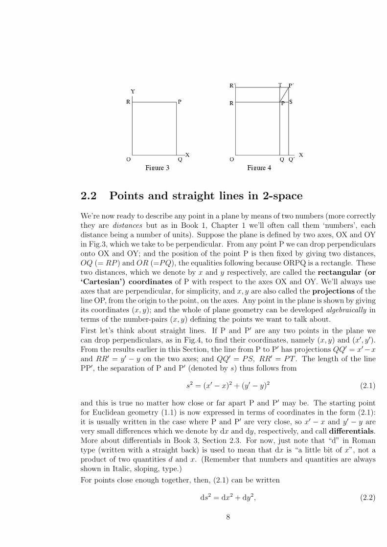
We’re now ready to describe any point in a plane by means of two numbers (more correctlythey are distances but as in Book 1, Chapter 1 we’ll often call them ‘numbers’, eachdistance being a number of units). Suppose the plane is defined by two axes, OX and OYin Fig.3, which we take to be perpendicular. From any point P we can drop perpendicularsonto OX and OY; and the position of the point P is then fixed by giving two distances,OQ (= RP ) and OR (=PQ), the equalities following because ORPQ is a rectangle. Thesetwo distances, which we denote by x and y respectively, are called the rectangular (or‘Cartesian’) coordinates of P with respect to the axes OX and OY. We’ll always useaxes that are perpendicular, for simplicity, and x, y are also called the projections of theline OP, from the origin to the point, on the axes. Any point in the plane is shown by givingits coordinates (x, y); and the whole of plane geometry can be developed algebraically interms of the number-pairs (x, y) defining the points we want to talk about.

First let’s think about straight lines. If P and P′ are any two points in the plane wecan drop perpendiculars, as in Fig.4, to find their coordinates, namely (x, y) and (x′, y′).From the results earlier in this Section, the line from P to P′ has projections QQ′ = x′−xand RR′ = y′ − y on the two axes; and QQ′ = PS, RR′ = PT . The length of the linePP′, the separation of P and P′ (denoted by s) thus follows from

s2 = (x′ − x)2 + (y′ − y)2 (2.1)

and this is true no matter how close or far apart P and P′ may be. The starting pointfor Euclidean geometry (1.1) is now expressed in terms of coordinates in the form (2.1):it is usually written in the case where P and P′ are very close, so x′ − x and y′ − y arevery small differences which we denote by dx and dy, respectively, and call differentials.More about differentials in Book 3, Section 2.3. For now, just note that “d” in Romantype (written with a straight back) is used to mean that dx is “a little bit of x”, not aproduct of two quantities d and x. (Remember that numbers and quantities are alwaysshown in Italic, sloping, type.)

For points close enough together, then, (2.1) can be written

ds2 = dx2 + dy2, (2.2)

8

which is called the ‘fundamental metric form’. In Euclidean space, the ‘sum-of-squares’form is true whether the separation of two points is large or small: but if you are makinga map you must remember that the surface of the earth is curved – so you can use (2.2)for small distances (e.g. your town) but not for large distances – your country. (Strictlyspeaking, (2.2) is only true ‘in the limit’ (see Book 1, Chapter 4) when the distancesgo to zero.) Space may be only locally Euclidean. Within the last hundred years ourideas about space have changed a lot, but in everyday life Euclidean geometry still servesperfectly well.

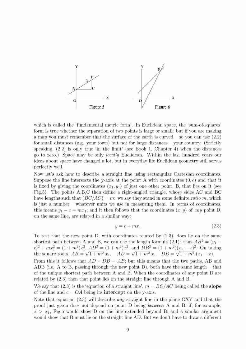
Now let’s ask how to describe a straight line using rectangular Cartesian coordinates.Suppose the line intersects the y-axis at the point A with coordinates (0, c) and that itis fixed by giving the coordinates (x1, y1) of just one other point, B, that lies on it (seeFig.5). The points A,B,C then define a right-angled triangle, whose sides AC and BChave lengths such that (BC/AC) = m: we say they stand in some definite ratio m, whichis just a number – whatever units we use in measuring them. In terms of coordinates,this means y1 − c = mx1; and it then follows that the coordinates (x, y) of any point D,on the same line, are related in a similar way:

y = c + mx. (2.3)

To test that the new point D, with coordinates related by (2.3), does lie on the sameshortest path between A and B, we can use the length formula (2.1): thus AB2 = (y1 −c)2 + mx2

1 = (1 + m2)x21, AD2 = (1 + m2)x2, and DB2 = (1 + m2)(x1 − x)2. On taking

the square roots, AB =√

1 + m2 x1, AD =√

1 + m2 x, DB =√

1 + m2 (x1 − x).

From this it follows that AD + DB = AB; but this means that the two paths, AB andADB (i.e. A to B, passing through the new point D), both have the same length – thatof the unique shortest path between A and B. When the coordinates of any point D arerelated by (2.3) then that point lies on the straight line through A and B.

We say that (2.3) is the ‘equation of a straight line’, m = BC/AC being called the slopeof the line and c = OA being its intercept on the y-axis.

Note that equation (2.3) will describe any straight line in the plane OXY and that theproof just given does not depend on point D being between A and B: if, for example,x > x1, Fig.5 would show D on the line extended beyond B; and a similar argumentwould show that B must lie on the straight line AD. But we don’t have to draw a different

9

picture for every possible case: if x, y refer to points on the left of the y-axis, or beneaththe x-axis, they will simply take negative values – and, as the laws of algebra hold for anynumbers, our results will always hold good.

Sometimes two lines in a plane will cross, meeting at some point P, as in Fig.6. Whetherthey do or not is an important question – which was the starting point for all of Euclid’sgreat work.

2.3 When and where will two

straight lines meet?

Let’s now look again at Euclid’s ‘parallel axiom’ – that two parallel straight lines nevermeet. What does it mean in algebra?

Suppose the two lines have equations like (2.3) but with different values of slope (m) andintercept (c): let’s say

y = c1 + m1x, y = c2 + m2x. (2.4)

In Fig.6 two such lines cross at the point P. How can we find it? The first equation in(2.4) relates the x and y coordinates of any point on Line 1, while the second equationdoes the same for any point on Line 2. At a crossing point, the same values must satisfyboth equations, which are then called simultaneous equations (both must hold at thesame time). It is easy to find such a point in any given case: thus, if m1 = 1, m2 = 2 andc1 = 1, c2 = −1, the values of x and y must be such that

y = 1 + x and y = −1 + 2x,

which arise by putting the numerical values in the two equations. Thus, we ask that1 + x = −1 + 2x at the crossing point; and this gives (see the Exercises in Book 1,Chapter 3) x = 2, with a related value of y = 1 + x = 3. This situation is shown in Fig.6,Point P being (2,3). If, instead, we took the second line to have the same slope (m2 = 2)but with c2 = 3, the result would be x = −2, y = −1. Try to get this result by yourself.

Finally, suppose the two lines have the same slope, m1 = m2 = m. In this case (x, y) atthe crossing point must be such that

y = c1 + mx = c2 + mx,

which can be true only if c1 = c2, whatever the common slope of the two lines: but thenthe two lines would become the same (same slope and same intercept) – there would beonly one! All points on either line would be ‘crossing points’. As long as m1 6= m2 wecan find a true crossing point for c1 6= c2; but as m1 and m2 become closer and closer thedistance to the crossing point becomes larger and larger. This ‘Point 3’ can’t be shownin Fig.6 – it is ‘the point at infinity’ !

This simple example is very important: it shows how an algebraic approach to geometry,based on the idea of distance and the metric (1.1), can lead to general solutions of geo-metrical problems, without the need to draw pictures for all possible situations; and it

10

shows that Euclid’s famous axiom, that parallel lines never meet, then falls out as a firstresult.

Before going on, let’s look at one other simple shape in 2-space – the circle which theancients thought was the most perfect of all shapes. It’s easy enough to draw a perfectcircle: you just hammer a peg into the ground and walk round it with some kind ofmarker, attached to the peg by a tightly stretched piece of string – the marker will markout a circle! But how do you describe it in algebra?

Let’s take the peg as origin O and the marker as point P, with coordinates x, y, say. Thenif your string has length l, and you keep it tight, you know that the distance OP (thethird side of a right-angled triangle, the other sides having lengths x and y) will alwaysbe the same – always l. But with the sum-of-squares metric this means

x2 + y2 = l2 = constant, (2.5)

however x and y may change. We say this is the “equation of a circle” with its centre atthe origin O; just as (2.4) was the equation of a straight line, with a given slope (m) andcrossing the y-axis at a certain point (y = c). The equation of the circle is of the ‘seconddegree’ (x and y being raised to the power 2); while that of the line is of the ‘first degree’or linear. In the Exercises and in other Chapters you’ll find many more examples.

Exercises

1) Suppose the corners of the rectangle in Fig.3 are at the points O(0,0), Q(3,0), P(3,4),R(0,4) and draw the straight line y = 1

2x. At what point does it meet the side QP? (Any

point on QP must have x = 3. So you only need to choose y.)

2) What happens if the line through the origin in Ex.1 is changed to y = 2x? (The pointfound in Ex.1 lies between Q and P: it is an internal point. The new point will lie on QPextended (beyond P): it is an external point, lying outside QP.)

3) Repeat Exercises 1 and 2, using in turn the lines

y = 3− 12x, y = 3− 2x, y = −3 + 1

2x, y = −3 + 2x,

and describe your results.

4) Instead of using equation (2.3), take y = 2 + 12x2 and draw the curve of y against x.

The new equation describes a parabola. Find values of x and y that fit the equation,using, in turn, the values x = −3,−2,−1, 0, +1, +2, +3 and ‘plot’ them (i.e. mark thepoints in a Figure and join them by a curved line.)

Find the points where the straight lines in Ex.3 cross the parabola (you need to knowhow to solve a quadratic equation – see Section 5.3 of Book 1) and show your results in aFigure.

Note In all the Exercises x, y, etc. are represented in the Figures as distances, so eachstands for a number of units ; but the size of the unit doesn’t matter, so it is not shown.

11

Chapter 3

Area and angle

3.1 What is area?

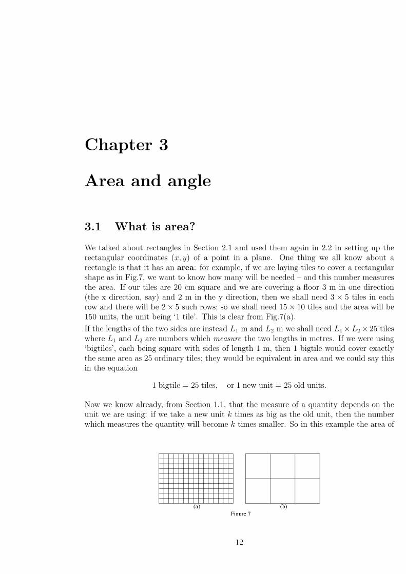
We talked about rectangles in Section 2.1 and used them again in 2.2 in setting up therectangular coordinates (x, y) of a point in a plane. One thing we all know about arectangle is that it has an area: for example, if we are laying tiles to cover a rectangularshape as in Fig.7, we want to know how many will be needed – and this number measuresthe area. If our tiles are 20 cm square and we are covering a floor 3 m in one direction(the x direction, say) and 2 m in the y direction, then we shall need 3 × 5 tiles in eachrow and there will be 2× 5 such rows; so we shall need 15× 10 tiles and the area will be150 units, the unit being ‘1 tile’. This is clear from Fig.7(a).

If the lengths of the two sides are instead L1 m and L2 m we shall need L1×L2× 25 tileswhere L1 and L2 are numbers which measure the two lengths in metres. If we were using‘bigtiles’, each being square with sides of length 1 m, then 1 bigtile would cover exactlythe same area as 25 ordinary tiles; they would be equivalent in area and we could say thisin the equation

1 bigtile = 25 tiles, or 1 new unit = 25 old units.

Now we know already, from Section 1.1, that the measure of a quantity depends on theunit we are using: if we take a new unit k times as big as the old unit, then the numberwhich measures the quantity will become k times smaller. So in this example the area of

12

the room will be A = 150 tiles = (150/25) bigtiles, the 6 bigtiles corresponding to thearea in ‘square metres’ of the 3 m × 2 m rectangle. This is shown in Fig.7(b): 6 bigtilesjust fit.

With the metre as the standard unit of length we see that the unit of area is 1 m2. So ifthe unit of length is multiplied by k, the measure of length will be divided by k; but theunit of area will be multiplied by k2 and the measure of area will be divided by k2. Weusually say that area has the “dimensions of length squared” or, in symbols, [area] =L2 (read as “the dimensions of area are el squared”). When we use symbols to stand forquantities we must always be careful to get the units right as soon as we use numbers tomeasure them!

The rectangle is a particular ‘shape’ with certain properties, like its area and the lengthof a side (i.e. the distance between two neighbouring corners). If we move it to anotherposition in space, such properties do not change – they belong to the object. An importantthing about the metric axiom (2.2) is that it means all distances will be left unchanged,or invariant, when we move an object without bending it or cutting it – an operationwhich is called a transformation. From this fact we can find the areas of other shapes.Two are specially important; the triangle 4, which has only three sides, and the circle ©,which has one continuous side (called its perimeter) at a fixed distance from its centre.

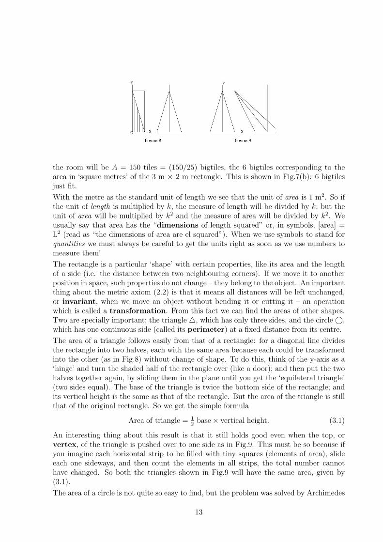
The area of a triangle follows easily from that of a rectangle: for a diagonal line dividesthe rectangle into two halves, each with the same area because each could be transformedinto the other (as in Fig.8) without change of shape. To do this, think of the y-axis as a‘hinge’ and turn the shaded half of the rectangle over (like a door); and then put the twohalves together again, by sliding them in the plane until you get the ‘equilateral triangle’(two sides equal). The base of the triangle is twice the bottom side of the rectangle; andits vertical height is the same as that of the rectangle. But the area of the triangle is stillthat of the original rectangle. So we get the simple formula

Area of triangle = 12

base× vertical height. (3.1)

An interesting thing about this result is that it still holds good even when the top, orvertex, of the triangle is pushed over to one side as in Fig.9. This must be so because ifyou imagine each horizontal strip to be filled with tiny squares (elements of area), slideeach one sideways, and then count the elements in all strips, the total number cannothave changed. So both the triangles shown in Fig.9 will have the same area, given by(3.1).

The area of a circle is not quite so easy to find, but the problem was solved by Archimedes

13

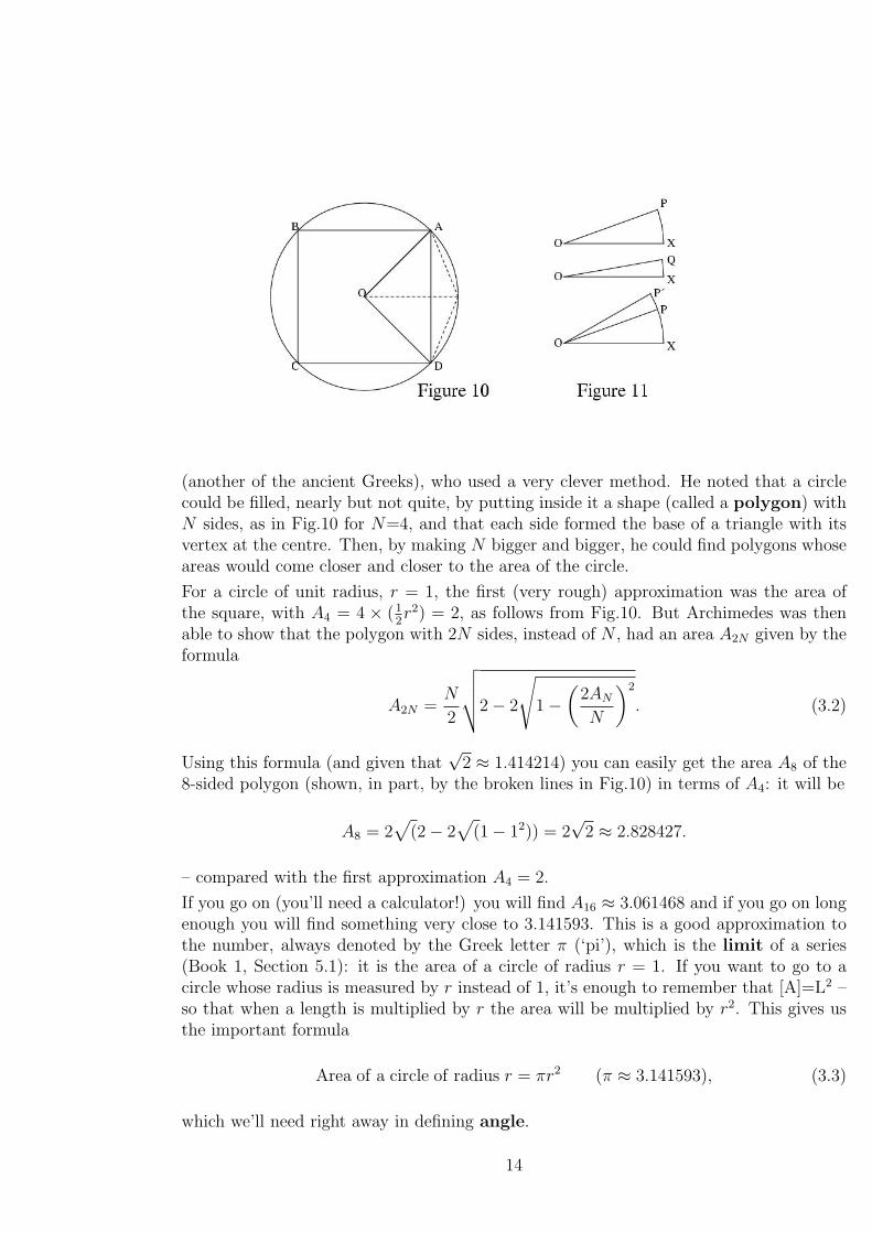
(another of the ancient Greeks), who used a very clever method. He noted that a circlecould be filled, nearly but not quite, by putting inside it a shape (called a polygon) withN sides, as in Fig.10 for N=4, and that each side formed the base of a triangle with itsvertex at the centre. Then, by making N bigger and bigger, he could find polygons whoseareas would come closer and closer to the area of the circle.

For a circle of unit radius, r = 1, the first (very rough) approximation was the area ofthe square, with A4 = 4 × (1

2r2) = 2, as follows from Fig.10. But Archimedes was then

able to show that the polygon with 2N sides, instead of N , had an area A2N given by theformula

A2N =N

2

√√√√2− 2

√1−

(2AN

N

)2

. (3.2)

Using this formula (and given that√

2 ≈ 1.414214) you can easily get the area A8 of the8-sided polygon (shown, in part, by the broken lines in Fig.10) in terms of A4: it will be

A8 = 2√

(2− 2√

(1− 12)) = 2√

2 ≈ 2.828427.

– compared with the first approximation A4 = 2.

If you go on (you’ll need a calculator!) you will find A16 ≈ 3.061468 and if you go on longenough you will find something very close to 3.141593. This is a good approximation tothe number, always denoted by the Greek letter π (‘pi’), which is the limit of a series(Book 1, Section 5.1): it is the area of a circle of radius r = 1. If you want to go to acircle whose radius is measured by r instead of 1, it’s enough to remember that [A]=L2 –so that when a length is multiplied by r the area will be multiplied by r2. This gives usthe important formula

Area of a circle of radius r = πr2 (π ≈ 3.141593), (3.3)

which we’ll need right away in defining angle.

14

3.2 How to measure angles

How can we measure the ‘angle’ between two intersecting straight lines when they areneither perpendicular nor parallel – when they simply ‘point in different directions’. Theslope m of a line is one such number, for it fixes the direction of the line AB in Fig.5relative to AC, which is parallel to the x-axis. We say that AB ‘makes an angle’ with ACand call m(= BC/AC) the tangent of the angle. This ratio is obtained easily for anypair of lines by dropping a perpendicular from a point on one of them to the other; andit also follows easily that it does not matter which line is taken first. Two other ratios,BC/AB and AC/AB, also give a simple arithmetic measure of the same angle: they arecalled, respectively, the sine and the cosine of the angle. There is, however, a singlenumber which gives a more convenient measure of the angle – ‘circular measure’, since itrelates directly to the circle. To get this we must think about combining angles.

Just as two points define a linear displacement which brings the first into coincidence withthe second; two straight lines, with one point in common, define an angular displacement,or a rotation, which brings the first into coincidence with the second. The rotation angleis given a sign, positive (for anti-clockwise rotation) or negative (for clockwise) – forrotations in the two opposite senses are clearly different. Just as two linear displacementsare called equal if their initial and final points can be put in coincidence (by sliding themabout in the plane), we call two angular displacements equal if their initial and final linescan be brought into coincidence. And just as two linear displacements can be combinedby making the end point of one the starting point of the next, we can combine two angulardisplacements by making the end line of one the starting line of the next. These ideaswill be clear on looking at Fig.11. Angles are named by giving three letters: the first isthe end point of the initial line; the last is the end point after rotation; and the middleletter is the point that stays fixed. The sum of the angles XOP and XOQ is the angleXOP′, obtained by taking OP as the starting line for the second angle, POP′, which ismade equal to XOQ.

After saying what we mean by ‘combination’ and ‘equality’ of angles, we look for an‘identity’ (in the algebra of rotations) and the ‘inverse’ of any angle, ideas which are oldfriends from Book 1. The ‘identity’ is now “don’t do anything at all (or rotate the initialline through an angle zero)”; and the ‘inverse’ of an angle is obtained simply by changingthe sense of the rotation – clockwise rotation followed by anti-clockwise rotation of thesame amount is equal to no rotation at all! If we write R for a positive rotation and R−1

for its inverse (negative rotation). this means

RR−1 = R−1R = I.

Next we must agree on how to measure angles. There is a ‘practical’ method, which startsfrom the fact that rotation of the line OP through a complete circle around the point O,let’s call it 1 ‘turn’, is the same as doing nothing. The ‘degree’ is a small angle, suchthat 360 degrees = 1 turn; and the angle between two lines in a plane can therefore bemeasured by a number (of degrees) lying between 0 and 360. Angles, unlike distances(which can be as big as you like), are thus bounded – since we can’t tell the differencebetween angles that differ only by 360 degrees (or any multiple of 360). This doesn’t mean

15

that angular displacement is bounded: we all know that, in turning a screw, for example,every turn (rotation through 360 degrees) is important; and it can be repeated again andagain to get bigger and bigger rotation angles. It is only the angle between two lines ina plane that is bounded: in the case of a screw, rotation has an effect outside the planeand it is then useful to talk about rotations through angles greater than 360 degrees.

A more fundamental way of measuring angles follows from the equation (3.3) for the areaof a circle. If we use θ to denote the angle XOP in Fig.11 (angles are usually namedusing Greek letters and θ is called ‘theta’), then the ‘circular measure’ of θ is the ratioof two lengths: θ = arc/radius, where ‘arc’ is the length of the part of the circle betweenpoint P and the x axis. This is a pure number, not depending on the unit of length,and gets as close as we wish to tan θ and sin θ as the angle becomes smaller and smaller.To find this number we write (3.3) in another form. The area of the whole circle (A)is the sum of the areas of a huge number of tiny triangles, each one with a small areaa ≈ 1

2arc × radius: so we find A = 1

2(whole arc) × radius where ‘whole arc’ means the

sum of all the tiny arcs, one for each triangle, as we go round the perimeter of the wholecircle. The length of this arc is the circumference of the circle. So what we have shownis that A = 1

2(Circumference × radius, and from (3.3) this gives the final result

Circumference of a circle = 2× Area ÷ radius = 2πr. (3.4)

Since the circumference is the ‘whole arc’, which is Θ × r (where Θ denotes the wholeangle turned through in going all round the circle), we can write Θ = 2π radians. Here,the radian is the ‘natural unit’ of angle and since, in terms of ‘degrees’ 2π radians = 360degrees, it follows from (3.3), that

1 radian ≈ 57.3 degrees. (3.5)

Usually, however, it is better to use radian measure: for example, two lines are perpen-dicular when the angle between them is π/2 and this does not depend on defining the‘degree’.

More on Euclid

Most of Euclid’s work was on plane figures (shapes such as triangles and rectangles thatlie in a plane). There’s so much of it that it would fill a whole book, so we just give oneor two definitions and key results to start things off:

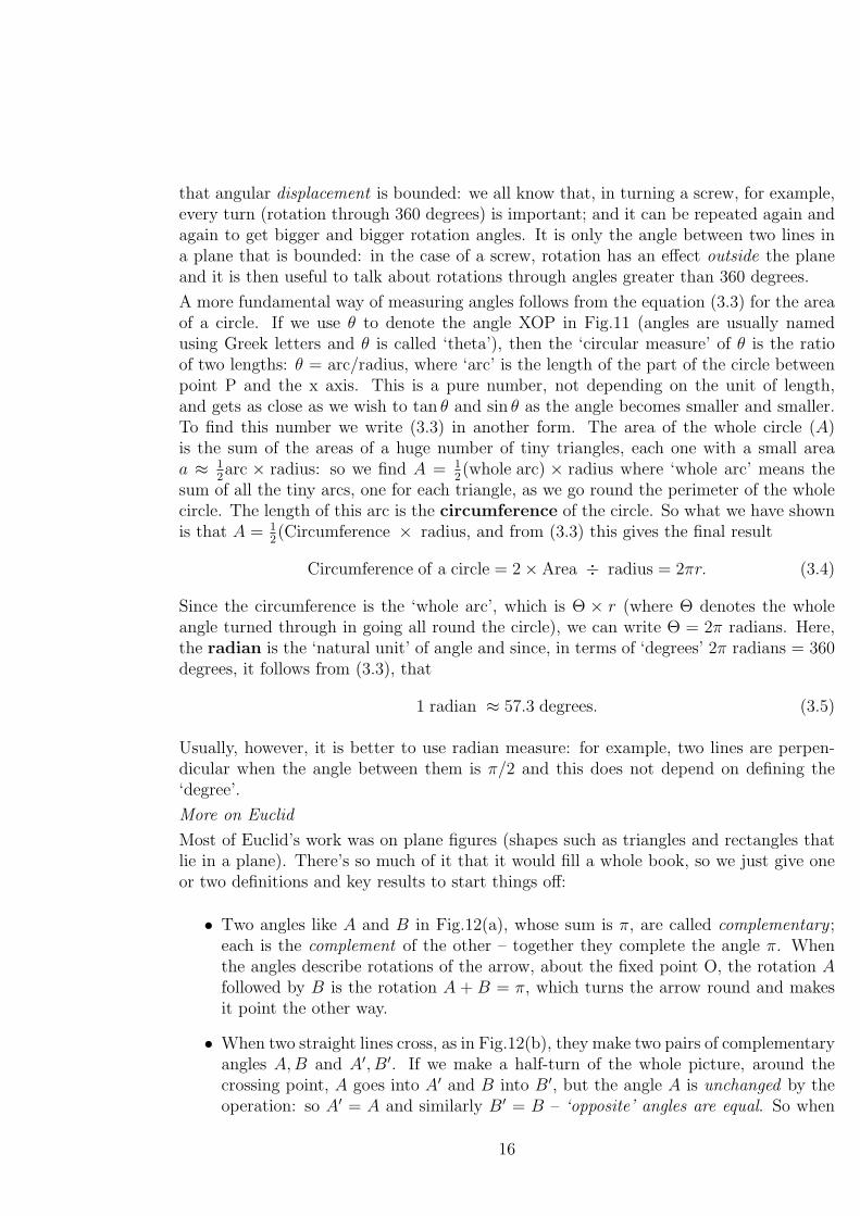
• Two angles like A and B in Fig.12(a), whose sum is π, are called complementary ;each is the complement of the other – together they complete the angle π. Whenthe angles describe rotations of the arrow, about the fixed point O, the rotation Afollowed by B is the rotation A + B = π, which turns the arrow round and makesit point the other way.

• When two straight lines cross, as in Fig.12(b), they make two pairs of complementaryangles A, B and A′, B′. If we make a half-turn of the whole picture, around thecrossing point, A goes into A′ and B into B′, but the angle A is unchanged by theoperation: so A′ = A and similarly B′ = B – ‘opposite’ angles are equal. So when

16

two lines cross they make two pairs of equal angles; and the different angles (A andB) are complementary.

• When a straight line crosses two parallel lines, as in Fig.12(c), it makes two otherpairs of equal angles A′ = A and B′ = B; for sliding the picture so as to send A intoA′ and B into B′ is another transfomation (see Section 3.1) that does not changethe angles. Such pairs of angles are called ‘alternate’.

• By adding another straight line to the last picture (Fig.12(c)) we make a triangle(Fig.12(d)) with three ‘internal’ angles, here called A, B, C. Now, from the last tworesults, A′ (being opposite to the angle alternate to A) is equal to A and similarlyC ′ = C. Also the sum of A′(= A), B, and C ′(= C) is the angle π in Fig.12(a). Itfollows that the sum of the angles inside any plane triangle is π radians (i.e. 180degrees or two right angles).

Euclid and his school proved a great number of other results of this kind, each one followingfrom those already obtained. All these theorems were numbered and collected and canstill be found in any textbook of geometry.

Note: The next Chapter contains difficult things, usually done only at university, butalso much that you will understand. Look at it just to see how many different ideas cometogether. Then come back to it when you’re ready – perhaps a year from now!

Exercises

1) Look at Figs.9,10 and then calculate the area of the 8-sided polygon, part of which isshown by the broken lines in Fig.10. Check that your result agrees with equation (3.2)when you put N = 4. (The polygon holds 2N triangles, all with the same area. Find thebase and the vertical height of each of them, taking the circle to have unit radius.)

2) Express all the angles in Fig.10 both in degrees and in radians.

17

Chapter 4

Rotations: bits and pieces

One of the great things about mathematics is that it contains so many ‘bits and pieces’which, again and again, can be put together like bricks, in building up new ideas andtheories. These small pieces are so useful that, once understood, they are never forgotten.In talking about angles and rotations we need to use vectors (Book 1, Section 3.2); thelaws of indices (Book 1, Section 4.2); the exponential series (Book 1, Section 5.1); complexnumbers (Book 1, Section 5.2); and the idea of rotation as an operator (as in Book 1,Section 6.1).

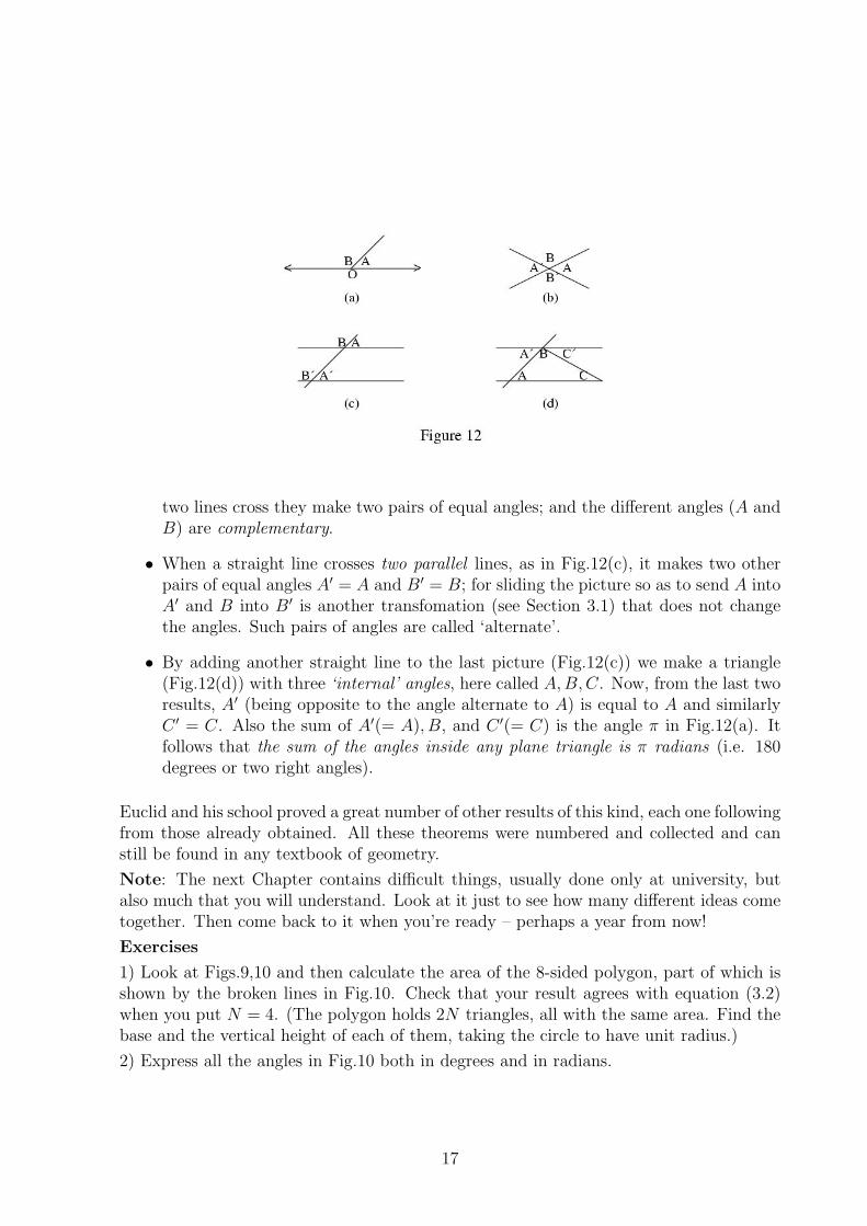
Let’s start with a vector pointing from the origin O to any point P, as in Fig.13. In arotation around O, any such vector is turned through some angle, let’s call it θ, and, asin Book 1, Section 6.1, we can think of this operation as the result of applying a rotationoperator Rθ. There is a law of combination for two such operators:

Rθ′Rθ = Rθ+θ′ ,

(don’t forget we agreed in Section 6.1 that the one on the right acts first) and for everyoperator Rθ there is an inverse operator, denoted by R−1

θ , with the property

RθR−θ = R−θRθ = I,

where I is the Identity operator (rotation through angle zero). These properties define agroup (Book 1, Section 6.1) with an infinite number of elements – since θ can take anyvalue between 0 and 2π (rotation through θ +2π not being counted as different from Rθ).We now want to put all this into symbols.

In 2-space any point P is found from its coordinates (x, y): to get there, starting fromthe origin (where x = 0, y = 0), you take x steps in the ‘x-direction’ (i.e. parallel to thex-axis) and y steps in the ‘y-direction’. In Book 1, Section 3.2 there was only one axisand e was used to mean 1 step along that axis; but now there are two kinds of step (e1

and e2, say), so we write, for the vector describing the displacement from O to P,

r = xe1 + ye2, (4.1)

where e1, e2 are along the two directions and r is called the ‘position vector’ of P. FromBook 1, Section 3.2, it’s clear that the order in which the steps are made doesn’t matter:

18

if x = 2 and y = 3 then r = e1 + e1 + e2 + e2 + e2 or, just as well, r = e2 + e1 + e2 + e2 + e1

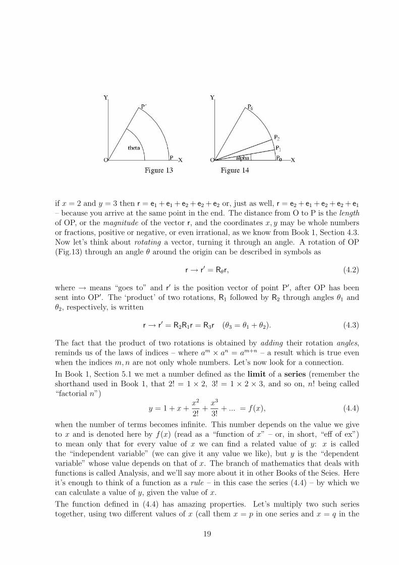
– because you arrive at the same point in the end. The distance from O to P is the lengthof OP, or the magnitude of the vector r, and the coordinates x, y may be whole numbersor fractions, positive or negative, or even irrational, as we know from Book 1, Section 4.3.Now let’s think about rotating a vector, turning it through an angle. A rotation of OP(Fig.13) through an angle θ around the origin can be described in symbols as

r → r′ = Rθr, (4.2)

where → means “goes to” and r′ is the position vector of point P′, after OP has beensent into OP′. The ‘product’ of two rotations, R1 followed by R2 through angles θ1 andθ2, respectively, is written

r → r′ = R2R1r = R3r (θ3 = θ1 + θ2). (4.3)

The fact that the product of two rotations is obtained by adding their rotation angles,reminds us of the laws of indices – where am × an = am+n – a result which is true evenwhen the indices m, n are not only whole numbers. Let’s now look for a connection.

In Book 1, Section 5.1 we met a number defined as the limit of a series (remember theshorthand used in Book 1, that 2! = 1 × 2, 3! = 1 × 2 × 3, and so on, n! being called“factorial n”)

y = 1 + x +x2

2!+

x3

3!+ ... = f(x), (4.4)

when the number of terms becomes infinite. This number depends on the value we giveto x and is denoted here by f(x) (read as a “function of x” – or, in short, “eff of ex”)to mean only that for every value of x we can find a related value of y: x is calledthe “independent variable” (we can give it any value we like), but y is the “dependentvariable” whose value depends on that of x. The branch of mathematics that deals withfunctions is called Analysis, and we’ll say more about it in other Books of the Seies. Hereit’s enough to think of a function as a rule – in this case the series (4.4) – by which wecan calculate a value of y, given the value of x.

The function defined in (4.4) has amazing properties. Let’s multiply two such seriestogether, using two different values of x (call them x = p in one series and x = q in the

19

other):

f(p)f(q) =

(1 + p +

p2

2!+ ...

) (1 + q +

q2

2!+ ...

)= 1 + (p + q) +

(p2

2!+ pq +

q2

2!

)+ ...

= 1 + (p + q) +(p + q)2

2!+ ... , (4.5)

– including terms only up to the ‘second degree’ (i.e. those with not more than twovariables multiplied together). The result seems to be just the same function (4.4), butwith the new variable x = p + q. And if you go on, always putting together products ofthe same degree, you’ll find the next terms are

(p + q)3/3! = (p3 + 3p2q + 3pq2 + q3)/3! (third degree)

and(p + q)4/4! = (p4 + 4p3q + 6p2q2 + 4pq3 + q4)/4! (degree 4.)

As you can guess, if we take more terms we’re going to get the result

f(p)f(q) = 1 + (p + q) +(p + q)2

2!+

(p + q)3

3!+ ... = f(p + q). (4.6)

To get a proof of this result is much harder: you have to look at all possible ways ofgetting products of the nth degree (n factors at a time) and then show that what you getcan be put together in the form (p + q)n/n!. So we’ll just accept (4.6) as a basic propertyof the exponential function, defined in (4.4) and often written as “exp x”.

From (4.6) we find, by putting p = q = x, that f(x)2 = f(2x); and on doing the sameagain f(x)3 = f(x)× f(2x) = f(3x). In fact

f(x)n = f(nx). (4.7)

This second basic property lets us define the nth power of a number even when n is notan integer ; it depends only on the series (2.14) and holds good when n is any kind ofnumber (irrational or even complex). Even more amazing, both (4.6) and (4.7) are truewhatever the symbols (x, p, q) may stand for – as long as they satisfy the usual laws ofcombination, including qp = pq (so that products can be re-arranged, as in getting theresult (4.6)).

In Book 1, Section 1.7, the (irrational) number obtained from (4.4) with x = 1 wasdenoted by e:

e = 1 + 1 +1

2+

1

6+

1

24+ . . . = 2.718281828 . . . (4.8)

and this gives us a ‘natural’ base for defining all real numbers. From (4.7), en = f(n) istrue for any n – not just for whole numbers but for any number. So changing n to x gives

ex = 1 + x +x2

2!+

x3

3!+ . . . , (4.9)

20

and the ‘laws of indices’ can now be written in general form as

exey = ex+y, (ex)y = exy. (4.10)

We’re now ready to go back to rotations in space! We know that rotations are combinedaccording to (4.3) and that every rotation Rθ is labelled by its rotation angle θ, which isjust a number. For some special values of θ, we also know what Rθ does to a vector in2-space. For example, R2πr = r, but Rπr = −r because rotating a vector through half aturn makes it point in the opposite direction, which means giving it a negative sign. Buthow can we describe a general rotation?

Any rotation can be made in small steps, for example in steps of 1 degree at a time, solet’s think of Rθ as the result of making n very small rotations through an angle α: soθ = nα and what we mean is that Rθ = (Rα)n, where we use the ‘power’ notation to meanthe product RαRα...Rα with n factors. So n becomes a measure of the rotation angle θin units of α; and if Rθ is followed by a rotation Rθ′ , with θ′ = mα, the result will be arotation through (m+n)α. Fig.14 gives a picture of the rotations which carry the positionvector of a point P0, on the x-axis, into P1 (1 step), P2 (2 steps), and so on – each stepbeing through a very small angle α (magnified here, so you can see it).

The rotation Rα sends the point P0, with position vector r = re1 + 0e2 (the componentsbeing x = r and y = 0 when r points along the x-axis), into P1 with r′ = Rα = x′e1 + y′e2.In general, the x- and y-components of any rotated vector (call them x, y for any rotationangle θ) are related to the sine and cosine of the angle turned through – as we know fromearlier in this Section. The definitions are cos α = x/r and sin α = y/r and the rotationleading to P1, with coordinates (x1, y1), thus gives

r1 = Rαr = x1e1 + y1e2 = r cos α e1 + r sin α e2. (4.11)

After repeating the operation n times we reach the vector ending on Pn: in short

rn = (Rα)nr = xne1 + yne2 = r cos(nα)e1 + r sin(nα)e2. (4.12)

Of course, we know how to get the sine and cosine from the picture (by measuringthe sides of a triangle) and we know their values for certain special angles like θ =2π, or π, or π/2, or even π/4; but what we really need is a way of calculating them forany angle θ (= nα).

To do this we start from the series (4.9), remembering that (4.10) gives us a way of findingits nth power just by writing nx in place of x (writing y = n because it stands for anynumber). And since x is also any number let’s experiment – putting x = iα, where i isthe ‘imaginary unit’ first introduced in Book 1, Section 5.2. The result is

eiα = 1 + iα− α2

2!− i

α3

3!+ ... (4.13)

where we’re using the fact that i2 = −1, i3 = i × i2 = −i, and so on. On collectingtogether the real terms (no i factors) we discover a new series:

Cα = 1− α2

2!+

α4

4!− ... (4.14)

21

and, on doing the same with the imaginary terms, find another series

Sα = α− α3

3!+

α5

5!− ... . (4.15)

Putting the two series together shows that

eiα = Cα + iSα (4.16)

and from (4.10) there’s a similar result when α is replaced by the large angle nα; so

einα = Cnα + iSnα, (4.17)

where Cnα and Snα are just like (4.14) and (4.15), but with nα instead of α.

Now look back at where we started: Equation (4.11) gives us the coordinates of P1

after rotating OP0 through a very small angle α and the (geometrically defined) valuesof sin α and cos α are, neglecting powers beyond α2, sin α ≈ α and cos α ≈ 1 − 1

2α2

– and these are the leading terms in the series (4.14) and (4.15)! For small angles,Cα → cos α, Sα → sin α. From these starting values we continue by (i) making morerotations, in steps of α, getting (4.12) after n steps; and (ii) multiplying eiα by the samefactor, in every step, to get einα after n steps. The two things go hand in hand. We takea bold step and say that

cos(nα) = Cnα, sin(nα) = Snα, (4.18)

are the algebraic expressions for the cosine and sine of any angle nα.

So we write, for any angle θ, the general results

cos θ = 1− θ2

2!+

θ4

4!− ... , sin θ = θ − θ3

3!+

θ5

5!− ... . (4.19)

And, from (4.17) with nα = θ,

eiθ = exp iθ = cos(θ) + i sin(θ) (4.20)

The above results lead to many others. Take an example: for any θ, we may square bothsides of equation (4.20) to obtain

e2iθ = (cos θ + i sin θ)2 = (cos θ)2 − (sin θ)2 + 2i sin θ cos θ.

But we also know thate2iθ = cos 2θ + i sin 2θ

and (from Book 1, Section 5.2) that two complex numbers are equal only when their realand imaginary parts are separately equal; so comparing the last two equations shows that

cos(2θ) = (cos θ)2 − (sin θ)2, sin(2θ) = 2 sin θ cos θ (4.21)

– knowing the sine and cosine of any angle you can get them very easily for twice the angle.For example, we know that sin(π/4) = cos(π/4) = 1

2

√2 (from the right-angled triangle

22

with sides of length 1, 1,√

2); so doubling the angle gives sin(π/2) = 1, cos(π/2) =0; doubling it again gives sin(π) = 0, cos(π) = −1; and yet again gives sin(2π) =1, cos(2π) = 0. The last result shows that the angle 2π (or 360 degrees) looks no differentfrom zero; and that every rotation through 2π gives us nothing new – the dependence ofsine and cosine on the angle is said to be periodic, they take the same values wheneverthe angle increases by 2π, called the period. In other words

e2πi = 1 (4.22)

– a connection between two irrational numbers (e, π) and the imaginary unit (i), almostbeyond belief! This is one of the most remarkable results in the whole of Mathematics.

The sine and cosine of the sum of any two angles follows in the same way as for twice theangle. Taking

exp i(θ1 + θ2) = exp iθ1 × exp iθ2,

using (4.20) and expanding the right-hand side, we find (try it yourself!)

cos(θ1 + θ2) = cos θ1 cos θ2 − sin θ1 sin θ2,

sin(θ1 + θ2) = sin θ1 cos θ2 + cos θ1 sin θ2. (4.23)

That’s all you need to know about angles – the rest you can do for yourself! A longtime ago, in school, when all of geometry was done the way Euclid did it, we had tolearn all these results (and many more) by heart – chanting them over and over again –and all because the Pythagoreans threw away their great discovery of algebraic geometry,leaving it for the French mathematician Rene Descartes (1596-1650) to re-discover morethan a thousand years later! Now you can get such results whenever you need them,remembering only the laws of indices and doing some simple algebra.

Exercises

1) Get the results labelled “(third degree)” and “(fourth degree)”, just after equation(4.5), by multiplying together the results you already know.

2) Obtain the results (4.13) to (4.20) by starting from (4.9) and working through all thedetails.

3) Starting from (4.23), find expressions for cos(θ1−θ2), sin(θ1−θ2), cos 2θ, sin 2θ, cos 3θ,sin 3θ.

23

Chapter 5

Three-dimensional space

5.1 Planes and boxes in 3-space – coordinates

As we all know, from birth, the real ‘physical’ space we live in is not a 2-space, or plane,in which a point is specified by giving two numbers to define its position. There are points‘above’ and ‘below’ any plane; and to define their positions we’ll need a third number – totell us how far up or how far down. Again, as in Section 1.2, we’ll refer a point to a set ofperpendicular axes, meeting at a point O – the origin – but now there will be three axesinstead of two. Up to now, we’ve been talking about plane geometry; but now we turnto 3-space and to solid geometry. The basic ideas, however, are not much different: westart from an axiom, just like that we used in 2-space, referring to the shortest distancebetween points; then we set up a few theorems from which all of solid geometry can bederived by purely algebraic reasoning. Of course, we won’t do all of it – just enough tomake us feel sure that it can be done.

According to the first Axiom (Section 1.2) a straight line is the unique shortest pathbetween two points. And from the definition of a plane (Section 1.2) it follows that if twoplanes intersect, then they cut each other in a straight line – for if any two points A andB are common to both planes then there is a unique straight line AB and all the pointson AB lie at the same time in both planes (i.e. AB, which may be as long as we wish, isthe line in which the planes intersect).

From this conclusion we can go to a first theorem:

Theorem. If a straight line is perpendicular to two others, which it meets ata common point, then it is perpendicular to all others in the same plane andpassing through the same point. It is then perpendicular to the plane.

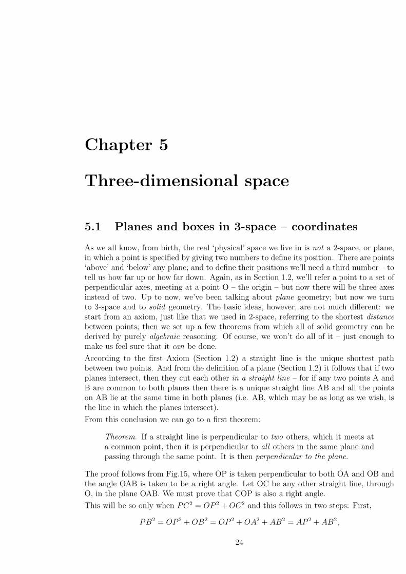
The proof follows from Fig.15, where OP is taken perpendicular to both OA and OB andthe angle OAB is taken to be a right angle. Let OC be any other straight line, throughO, in the plane OAB. We must prove that COP is also a right angle.

This will be so only when PC2 = OP 2 + OC2 and this follows in two steps: First,

PB2 = OP 2 + OB2 = OP 2 + OA2 + AB2 = AP 2 + AB2,

24

and therefore PAB is also a right angle. Then, second, we have

PC2 = PA2 + AC2 = OA2 + OP 2 + AC2 = OC2 + OP 2.

This proves the theorem.

Two other simple results follow:

• The perpendicular from a point to a plane is the shortest path from the point toany point in the plane.

• If a straight line is perpendicular to two others, which meet it at some point, thenthe two others lie in a plane.

These are ‘corollaries’ to the theorem, the second one being the converse of the theorem– saying it the other way round.

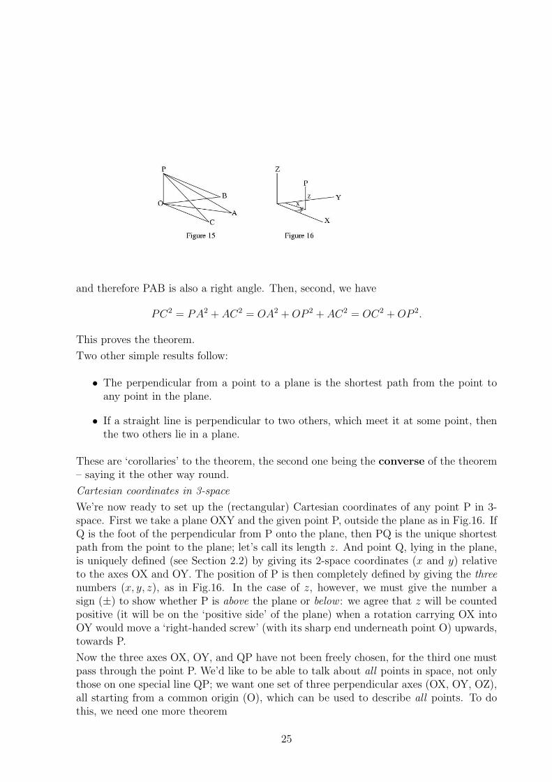
Cartesian coordinates in 3-space

We’re now ready to set up the (rectangular) Cartesian coordinates of any point P in 3-space. First we take a plane OXY and the given point P, outside the plane as in Fig.16. IfQ is the foot of the perpendicular from P onto the plane, then PQ is the unique shortestpath from the point to the plane; let’s call its length z. And point Q, lying in the plane,is uniquely defined (see Section 2.2) by giving its 2-space coordinates (x and y) relativeto the axes OX and OY. The position of P is then completely defined by giving the threenumbers (x, y, z), as in Fig.16. In the case of z, however, we must give the number asign (±) to show whether P is above the plane or below : we agree that z will be countedpositive (it will be on the ‘positive side’ of the plane) when a rotation carrying OX intoOY would move a ‘right-handed screw’ (with its sharp end underneath point O) upwards,towards P.

Now the three axes OX, OY, and QP have not been freely chosen, for the third one mustpass through the point P. We’d like to be able to talk about all points in space, not onlythose on one special line QP; we want one set of three perpendicular axes (OX, OY, OZ),all starting from a common origin (O), which can be used to describe all points. To dothis, we need one more theorem

25

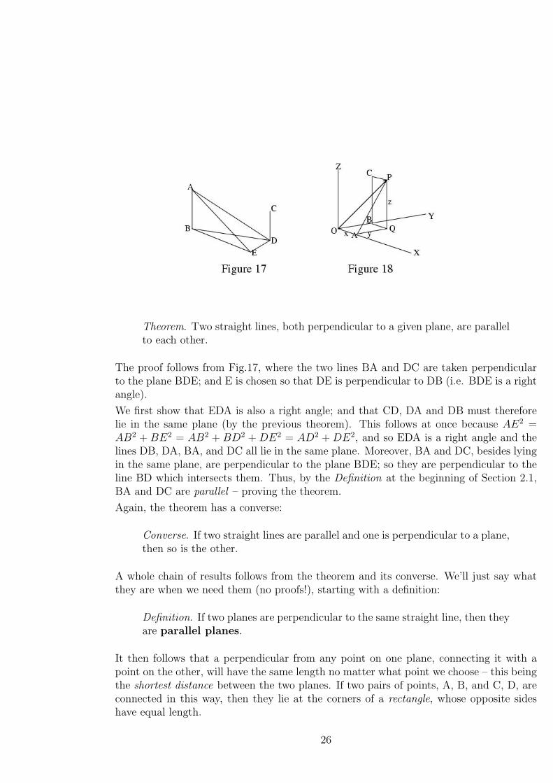
Theorem. Two straight lines, both perpendicular to a given plane, are parallelto each other.

The proof follows from Fig.17, where the two lines BA and DC are taken perpendicularto the plane BDE; and E is chosen so that DE is perpendicular to DB (i.e. BDE is a rightangle).

We first show that EDA is also a right angle; and that CD, DA and DB must thereforelie in the same plane (by the previous theorem). This follows at once because AE2 =AB2 + BE2 = AB2 + BD2 + DE2 = AD2 + DE2, and so EDA is a right angle and thelines DB, DA, BA, and DC all lie in the same plane. Moreover, BA and DC, besides lyingin the same plane, are perpendicular to the plane BDE; so they are perpendicular to theline BD which intersects them. Thus, by the Definition at the beginning of Section 2.1,BA and DC are parallel – proving the theorem.

Again, the theorem has a converse:

Converse. If two straight lines are parallel and one is perpendicular to a plane,then so is the other.

A whole chain of results follows from the theorem and its converse. We’ll just say whatthey are when we need them (no proofs!), starting with a definition:

Definition. If two planes are perpendicular to the same straight line, then theyare parallel planes.

It then follows that a perpendicular from any point on one plane, connecting it with apoint on the other, will have the same length no matter what point we choose – this beingthe shortest distance between the two planes. If two pairs of points, A, B, and C, D, areconnected in this way, then they lie at the corners of a rectangle, whose opposite sideshave equal length.

26

5.2 Describing simple objects in 3-space

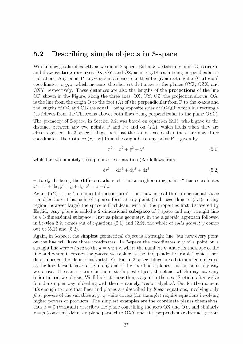
We can now go ahead exactly as we did in 2-space. But now we take any point O as originand draw rectangular axes OX, OY, and OZ, as in Fig.18, each being perpendicular tothe others. Any point P, anywhere in 3-space, can then be given rectangular (Cartesian)coordinates, x, y, z, which measure the shortest distances to the planes OYZ, OZX, andOXY, respectively. These distances are also the lengths of the projections of the lineOP, shown in the Figure, along the three axes, OX, OY, OZ: the projection shown, OA,is the line from the origin O to the foot (A) of the perpendicular from P to the x-axis andthe lengths of OA and QB are equal – being opposite sides of OAQB, which is a rectangle(as follows from the Theorems above, both lines being perpendicular to the plane OYZ).

The geometry of 2-space, in Section 2.2, was based on equation (2.1), which gave us thedistance between any two points, P and P′; and on (2.2), which holds when they areclose together. In 3-space, things look just the same, except that there are now threecoordinates: the distance (r, say) from the origin O to any point P is given by

r2 = x2 + y2 + z2 (5.1)

while for two infinitely close points the separation (dr) follows from

dr2 = dx2 + dy2 + dz2 (5.2)

– dx, dy, dz being the differentials, such that a neighbouring point P′ has coordinatesx′ = x + dx, y′ = y + dy, z′ = z + dz

Again (5.2) is the ‘fundamental metric form’ – but now in real three-dimensional space– and because it has sum-of-squares form at any point (and, according to (5.1), in anyregion, however large) the space is Euclidean, with all the properties first discovered byEuclid. Any plane is called a 2-dimensional subspace of 3-space and any straight lineis a 1-dimensional subspace. Just as plane geometry, in the algebraic approach followedin Section 2.2, comes out of equations (2.1) and (2.2), the whole of solid geometry comesout of (5.1) and (5.2).

Again, in 3-space, the simplest geometrical object is a straight line; but now every pointon the line will have three coordinates. In 2-space the coordinates x, y of a point on astraight line were related so the y = mx+c, where the numbers m and c fix the slope of theline and where it crosses the y-axis; we took x as the ‘independent variable’, which thendetermines y (the ‘dependent variable’). But in 3-space things are a bit more complicatedas the line doesn’t have to lie in any one of the coordinate planes – it can point any waywe please. The same is true for the next simplest object, the plane, which may have anyorientation we please. We’ll look at these things again in the next Section, after we’vefound a simpler way of dealing with them – namely, ‘vector algebra’. But for the momentit’s enough to note that lines and planes are described by linear equations, involving onlyfirst powers of the variables x, y, z, while circles (for example) require equations involvinghigher powers or products. The simplest examples are the coordinate planes themselves:thus z = 0 (constant) describes the plane containing the axes OX and OY, and similarlyz = p (constant) defines a plane parallel to OXY and at a perpendicular distance p from

27

the origin. In both cases any point in the plane is determined by giving values, any wewish, of the other variables x, y.

The simplest solid object (after the cube, which has six plane faces) is the sphere,corresponding to the circle in 2-space. It has a single curved surface and the coordinatesof any point on the surface are related by an equation of the second degree. The distanceof a point P(x, y, z) from the origin is given by

r2 = x2 + y2 + z2 (5.3)

and this distance (r) is the radius of the sphere, the same for all points on the surface.Thus (5.3) is the equation for the surface of a sphere centred on the origin. If you move thesphere (or the line or the plane) the equation will be more complicated. This is becauseour descriptions are based on choosing a set of axes that meet at the centre of the sphereand then using three distances (coordinates) to define every point; the set of axes is calleda reference frame. If we decide to change the reference frame, so that the origin is nolonger at the centre, then all the coordinates will have to be changed.

On the other hand, the objects we meet in 3-space have certain measurable properties(like length and area) which ‘belong’ to the object and do not depend in any way onhow we choose the reference frame: as already noted (Chapter 3) they are invariants.We’d like to keep our equations as simple and as close as possible to what we’re tryingto describe: a line, for example, is a vector and could be denoted by a single symbol –instead of a set of numbers that will change whenever we change the reference frame.We’ll see how to do this in the next Section.

5.3 Using vectors in 3-space

In ordinary algebraic number theory (Book 1, Chapter 4) we represented numbers bypoints on a straight line, or with the displacements which lead from an origin to thesepoints. The displacements are in fact vectors in a 1-space, each being a numericalmultiple of a unit ‘step’ which we called e; and any 1-vector a is written as a = ae, wherea is just a number saying ‘how many’ steps we take in the direction of e. Of course, if ais an integer, the displacement will lead to a point labelled by that integer; but we knowfrom Book 1 that this picture can be extended to the case where a is any real numberand a is the vector leading to its associated point in the pictorial representation. Therules for combining vectors in 1-space are known from Book 1: we get the sum of twodisplacements, a and b, by making them one after the other (the end point of the firstbeing the starting point for the second) and it doesn’t matter which way round we takethem. Thus

a + b = b + a, (5.4)

and if there are three vectors it doesn’t matter how we combine them,

(a + b) + c = a + (b + c). (5.5)

We can also multiply a vector by any real number, as in writing a as a number a of unitse: a = ae. Let’s try to do the same things in 3-space. There will now be three different

28

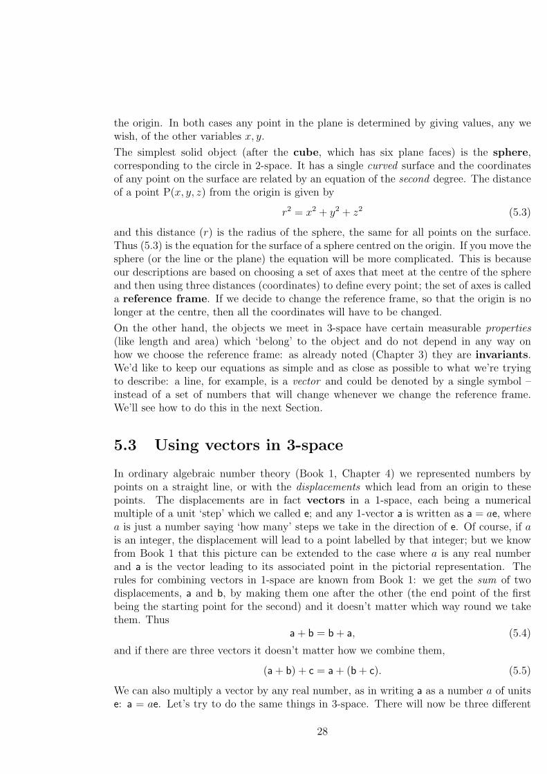
kinds of unit step – along the x-axis, the y-axis, and the z-axis – which we’ll call e1, e2, e3,respectively. They will be the basis vectors of our algebra and we take them to be ofunit length (being ‘unit steps’) A vector pointing from the origin O to point P(x, y, z)(i.e. with Cartesian coordinates x, y, z) will be denoted by r and written

r = xe1 + ye2 + ze3. (5.6)

This is really just a rule for getting from O to P: If the coordinates are integers e.g. x=3,y=2, z=6, this reads “take 3 steps of type e1, 2 of type e2 and 6 of type e3 – and you’ll bethere!” And the remarkable fact is that, even although the terms in (5.6) are in differentdirections, the order in which we put them together doesn’t make any difference: you cantake 2 steps parallel to the z-axis (type e3), then 2 steps parallel to the y-axis (type e2),3 more steps of type e1, and finally 4 steps of type e3 – and you’ll get to the same point.This is easy to see from Fig.19, remembering that (because the axes are perpendicular)space is being ‘marked out’ in rectangles, whose opposite sides are equal. In fact, therules (5.4) and (5.5) apply generally for vector addition.

An important thing to note is that in combining the terms in (5.6) the vectors must beallowed to ‘float’, as long as they stay parallel to the axes: they are called ‘free vectors’and are not tied to any special point in space. On the other hand, the position vectorr is defined as a vector leading from the origin O to a particular point P: it is a ‘boundvector’.

The numbers x, y, z in (5.6), besides being coordinates of the point P, are also compo-nents of its position vector. Any vector may be expressed in a similar form –

a = a1e1 + a2e2 + a3e3

b = b1e1 + b2e2 + b3e3,

etc. and addition of vectors leads to addition of corresponding components. Thus, re-arranging the terms in the sum,

a + b = (a1 + b1)e1 + (a2 + b2)e2 + (a3 + b3)e3. (5.7)

29

Similarly, multiplication of a vector by any real number c is expressed in component formby

ca = ca1e1 + ca2e2 + ca3e3. (5.8)

Finally, note that the vector algebra of Euclidean 3-space is very similar to the ordinaryalgebra of real numbers (e.g. Book 1, Chapter 3). There is a ‘unit under addition’ whichcan be added to any vector without changing it, namely 0 = 0e1 + 0e2 + 0e3; and everyvector a has an ‘inverse under addition’, denoted by −a = −a1e1 − a2e2 − a3e3, such that−a + a = 0.

5.4 Scalar and vector products

From two vectors, a, b, it’s useful to define special kinds of ‘product’, depending on theirlengths (a, b) and the angle between them (θ). (The length of a vector a is often writtenas a = |a| and called the modulus of a.)

Definition. The scalar product, written a · b, is defined by a · b = ab cos θ.

Definition. The vector product, written a×b, is defined by a×b = ab sin θ c,

where c is a new unit vector, normal (i.e. perpendicular) to the plane of a, band pointing so that rotating a towards b would send a right-handed screw inthe direction of c.

The ‘scalar’ product is just a number (in Physics a ‘scalar’ is a quantity not associatedwith any particular direction); but the vector product is connected with the area of thepiece of surface defined by the two vectors – and c points ‘up’ from the surface, so as toshow which is its ‘top’ side (as when we first set up the z-axis). Both products have theusual ‘distributive’ property, that is

(a + b) · c = a · c + b · c, (a + b)× c = a× c + b× c,

but, from its definition, the vector product changes sign if the order of the vectors isreversed (b× a = −a× b) – so whatever we do we must keep them in the right order.

The unit vectors e1, e2, e3 each have unit modulus, |e1| = |e2| = |e3| = 1; and each isperpendicular to the other two, e1 · e2 = e1 · e3 = e2 · e3 = 0. It follows that the scalarproduct between any pair of vectors a, b is, in terms of their components,

a · b = (a1e1 + a2e2 + a3e3) · (b1e1 + b2e2 + b3e3)

= a1b1e1 · e1 + . . . + a1b2e1 · e2 + . . . ,

where the dots mean ‘similar terms’; and from the properties of the unit vectors (above)this becomes

a · b = a1b1 + a2b2 + a3b3. (5.9)

30

When b = a we get a · a = a2 = a21 + a2

2 + a23 (the original sum-of-squares form for a

length); and for the position vector r of any point P we find

OP = r =√

x2 + y2 + z2. (5.10)

Similarly, for two vectors r, r′, the scalar product is

r · r′ = rr′ cos θ = xx′ + yy′ + zz′

and this tells us how to find the angle between any two vectors. Remember that x, y, z areprojections of r on the three coordinate axes, so x/r = cos α (α being the angle betweenr and the x-axis); and similarly for the second vector, x′/r′ = cos α′. The cosines of theangles between a vector and the three axes are usually called the direction cosines ofthe vector and are denoted by l,m, n. With this notation the equation above can bere-written as

cos θ = ll′ + mm′ + nn′ (5.11)

– a simple way of getting the angle θ, which applies for any two vectors in 3-space.

5.5 Some examples

To end this chapter it’s useful to look at a few examples of how you can describe points,lines, planes, and simple 3-dimensional shapes in vector language. By using vectors youcan often get the results you need much more easily than by drawing complicated diagramsand thinking of all the ‘special cases’ that can arise.

• Angles in a triangle In Section 1.2 we took the theorem of Pythagoras, for aright-angled triangle as the ‘metric axiom’. There are many theorems concernedwith triangles that we haven’t even mentioned; and many of them refer to a generaltriangle, with no special angles. Let’s take such a triangle, with vertices A,B,C,using the same letters to denote the corresponding angles A, B, C, and the smallletters a, b, c to denote the lengths of the sides opposite to angles A, B, C. We canalso use the special symbols a, b, c to mean the vectors pointing along the sides,following one another in the positive (anti-clockwise) direction. (Before going on,you should make a careful drawing of the triangle ABC, labelling the sides andangles. Then you’ll have the picture in your head.)

There are two basic ‘laws’ relating the sines and cosines of the angles. The first isvery easy to get: if you drop a perpendicular from vertex C onto the line throughA and B, calling its length h, then sin A = h/b, sin B = h/a; and so h = b sin A =a sin B. On dividing by ab we get (sin A/a) = (sin B/b). Taking vertex A next, youfind a similar result; and on putting them together you find

sin A

a=

sin B

b=

sin C

c. (5.12)

This is the ‘Law of Sines’ for any plane triangle.

31

Now note that the sum of the vectors a, b, c (displacements following each otherround the triangle and bringing you back to the starting point) is zero: a+b+c = 0.So a = −(b + c) and the squared length of a is

a2 = a · a = (b + c) · (a + c)

= a · a + b · b + 2a · b = b2 + c2 + 2b · c.

From the definition of the scalar product in Section 5.2, b · c = bc cos θ when bothvectors point away from the point of intersection: but that means turning c round,making it −c. The result you get, along with two others like it (obtained by takingvertex B in place of A, and then vertex C) give us the ‘Law of Cosines’:

a2 = b2 + c2 − 2bc cos A

b2 = c2 + a2 − 2ca cos B (5.13)

c2 = a2 + b2 − 2ca cos C.

• Vector equation of a straight line Suppose we want the line to pass through apoint A, with position vector a, and to be parallel to a given vector b – which canbe of unit length (b2 = b · b = 1). Then a general point on the line, P, with positionvector r, will be given by

r = a + sb (5.14)

where s is any variable number – and that’s the equation we need! If instead wewant the equation for a line passing through two points, A and B (position vectorsa, b), then we simply replace b in the last equation by the vector b− a, which pointsfrom A to B: the result is

r = a + s(b− a).

• Vector equation of a plane Suppose ON is a normal to the plane, drawn fromthe origin O to the foot of the perpendicular, N; and let n be a unit vector inthe direction ON, so ~ON = pn where p is the perpendicular distance from O tothe plane. If r is the position vector of P, any other point in the plane, then itsprojection (Section 5.2) on the line ON must have the same value p. In other words,

r · n = p (5.15)

will be the equation defining a plane, with unit normal n, at perpendicular distancep from the origin.

• Distance of a point from a plane The perpendicular distance from the origin toa point P in the plane, given by (5.15), is p = r · n. That from the origin to anyother point, P′ with position vector r′, will be p′ = r′ · n – where we’re thinking ofpoint P′ as being in some parallel plane (which will have the same normal n). Therequired distance is therefore

d = p′ − p = r′ · n− p

and this will be positive when P′ is above the given plane, going out from the originin the direction n.

32

• Intersection of two planes The angle θ between two planes means the anglebetween their normals; so it follows from

cos θ = n · n′,

n, n′ being the two unit normals. If θ is zero the planes will be parallel; but otherwisethey will intersect – somewhere, but where? A point (r) which lies on both planesmust satisfy both equations, r · n = p, r · n′ = p′. It will then lie on the line ofintersection; but if we multiply the two equations by any two numbers c and c′ andadd the results we’ll get

r · (cn− c′n′) = cp− c′p′.

And this is the equation of a plane with its normal in the direction cn − c′n′: itdescribes a plane through the line of intersection of the two given planes – whichone depending on the values we give to c and c′.

Now a vector dn + d′n′ (the numbers d, d′ to be chosen), starting from the origin,will contain the normals (n, n′) to both planes and will therefore cut the line ofintersection: we take it as the vector a in equation(5.14), choosing d and d′ so thatthe point will lie on both planes. Then we need only the direction, the unit vector bin (5.14), to fix the line. And since the line of intersection is perpendicular to bothnormals we can take b as the vector product n × n′ defined in Section 5.4. Puttingthings together, the equation of the line of intersection is

r = dn + d′n′ + sn× n′, (5.16)

where the value of s changes as you run along the line.

• Equation of a sphere We’ve already met the equation for a sphere centred onthe origin, in Section 5.2, in terms of Cartesian coordinates. Let’s now look at onecentred on the point C (position vector c), with radius R. The distance from C tothe surface is the length of the vector r − c and the condition for point r to lie onthe surface is thus |r − c|2 = R2. Thus, expanding,

r2 − 2r · c + (c2 −R2) = 0 (5.17)

and this is the equation of the sphere centred on point c.

• Intersection of a straight line and a sphere Suppose the line is given by (5.14)and the sphere by (5.17): the point r must satisfy both these conditions. If we putthe first in the second we get

(a− sb) · (a− sb)− 2(a− sb) · c + (c2 −R2) = 0.

This contains the first and second powers of the variable number s and will thereforebe a quadratic equation (Book 1, Section 5.3), which can be written as

As2 + Bs + C = 0,

33

whereA = b2 = 1, B = 2b · (a− c), C = a2 + c2 −R2 − 2a · c.

There will be two roots, both real numbers, when B2 > 4AC; and these values ofs fix the two points where the straight line meets the surface. If it happens thatB2 and 4AC are exactly equal, then the two points become one and the line justtouches the surface in a single point. The line is then a tangent to the sphere.

Exercises

1) Find a unit vector perpendicular to each of the vectors v1 = 2e1 − e2 + e3 and v2 =3e1 + 4e2 − e3. Calculate the angle between v1 and v2.

2) Find two vectors which make equal angles with e1, are perpendicular to each other,and are perpendicular to e1 + e2 + e3.

3) What is the vector equation of a straight line through the points e1 − 2e2 + e3 and3e3 − 2e2? And where does this line meet the plane which contains the origin and thepoints 4e2 and 2e1 + e2?

4) Show that the line joining the mid points of two sides of a triangle is parallel to thethird side and is of half its length.

5) Show that the three points whose position vectors are a, b, and 3a− 2b lie on the samestraight line.

6) Find the equation of the straight line passing through the point with position vector dand making equal angles with the vectors a, b, c.

7) Find the equation of the plane through the point 2e1 + 3e2− e3 which is perpendicularto the vector 3e1 − 4e2 + 7e3.

8) Show that the points e1− e2 + 3e3 and 3(e1 + e2 + e3) are each the same distance fromthe plane

r · (5e1 + 2e2 − 7e3) + 9 = 0,

but are on opposite sides of it.

34

Chapter 6

Area and volume: invariance

6.1 Invariance of lengths and angles

At the end of Section 5.2 we noted that the objects we meet in 3-space have properties‘of their own’ which don’t change if we move them around from one part of space toanother – as long as we don’t bend them or twist them or change their ‘natural’ shapes.The objects may be, for example, rods or sticks (with a length of their own; or plates(with an area); or bricks or buckets (with a volume). All such properties are invariantunder the transformations that simply move an object from one place to another. Andin the last Section we laid the foundations for describing invariance mathematically, byusing single symbols (vectors) to stand for elements of space: the separation of two pointsin an object, for example, is described by a vector d = d1e1 + d2e2 + d3e3, say, whoselength does not change when we move the object. In fact, such transformations havethe fundamental property of leaving invariant all distances and angles – which define theshape of the object. This was the property used by the Greeks in their development ofplane geometry – for example in comparing two triangles to see if they were exactly alike,meaning one could be placed on top of the other with all sides and angles matching. Theyused pictures, but here we’re using algebraic methods and working in three dimensions(solid geometry) rather than two; and it’s here that vectors are especially useful.

Let the position vectors of points P and Q, relative to an origin O and a set of unit vectorse1, e2, e3, be

p = p1e1 + p2e2 + p3e3 q = q2e1 + q2e2 + q2e3,

where (so as not to be confused) we use p1, p2, p3 for the components of p instead of x, y, z.

The vector pointing from P to Q (often written ~PQ) is the difference

~PQ = dPQ = q− p = (q1 − p1)e1 + (q2 − p2)e2 + (q3 − p3)e3.

The simplest transformation we can make is a translation, in which every point P ismoved into its image, P′, with position vector p′ = p + t, where t is a constant vector. Itis clear from Fig.20 that the vector from P′ to Q′ is just the same as that from P to Q,

35

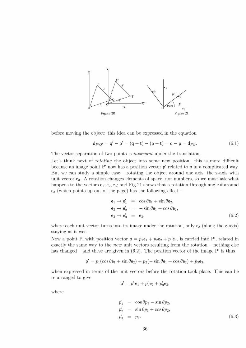
before moving the object: this idea can be expressed in the equation

dP ′Q′ = q′ − p′ = (q + t)− (p + t) = q− p = dPQ. (6.1)

The vector separation of two points is invariant under the translation.

Let’s think next of rotating the object into some new position: this is more difficultbecause an image point P′ now has a position vector p′ related to p in a complicated way.But we can study a simple case – rotating the object around one axis, the z-axis withunit vector e3. A rotation changes elements of space, not numbers, so we must ask whathappens to the vectors e1, e2, e3; and Fig.21 shows that a rotation through angle θ arounde3 (which points up out of the page) has the following effect –

e1 → e′1 = cos θe1 + sin θe2,

e2 → e′2 = − sin θe1 + cos θe2,

e3 → e′3 = e3, (6.2)

where each unit vector turns into its image under the rotation, only e3 (along the z-axis)staying as it was.

Now a point P, with position vector p = p1e1 + p2e2 + p3e3, is carried into P′, related inexactly the same way to the new unit vectors resulting from the rotation – nothing elsehas changed – and these are given in (6.2). The position vector of the image P′ is thus

p′ = p1(cos θe1 + sin θe2) + p2(− sin θe1 + cos θe2) + p3e3,

when expressed in terms of the unit vectors before the rotation took place. This can bere-arranged to give

p′ = p′1e1 + p′2e2 + p′3e3,

where

p′1 = cos θp1 − sin θp2,

p′2 = sin θp1 + cos θp2,

p′3 = p3. (6.3)

36

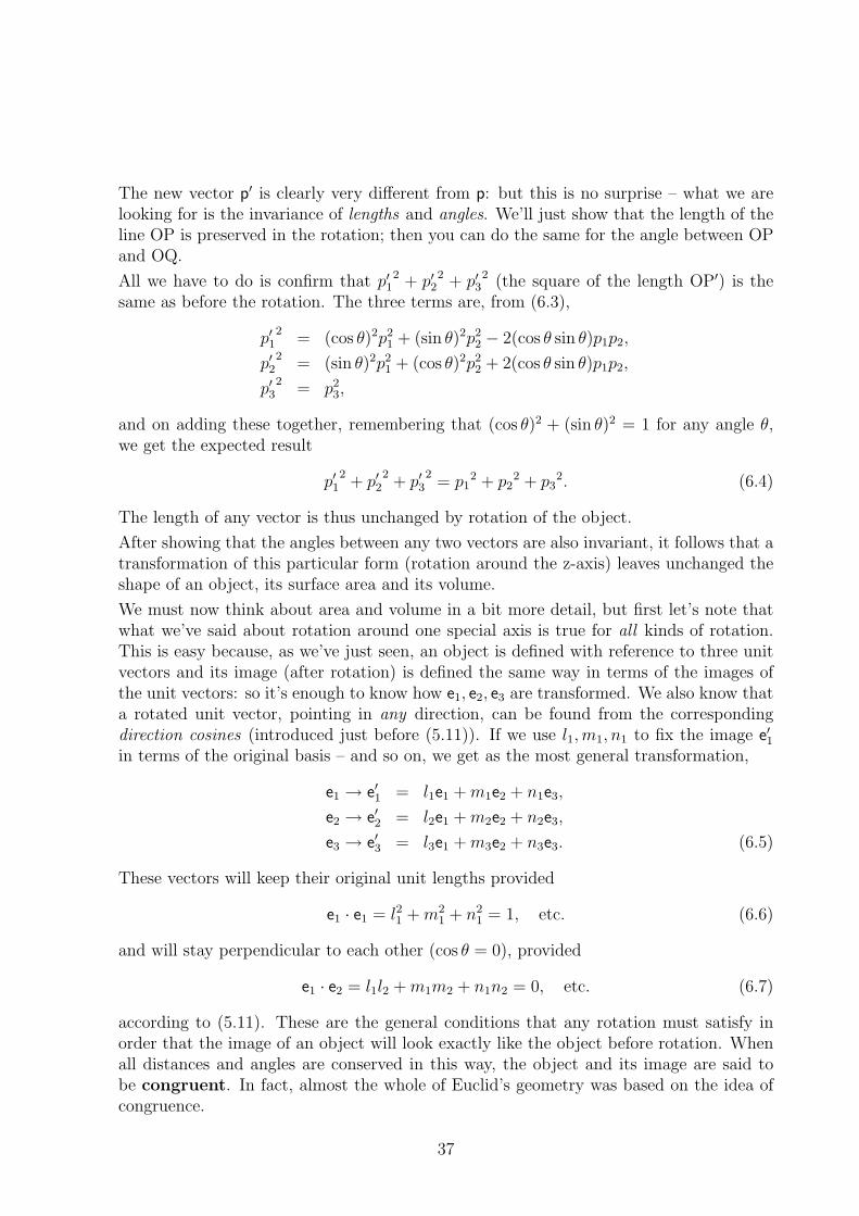
The new vector p′ is clearly very different from p: but this is no surprise – what we arelooking for is the invariance of lengths and angles. We’ll just show that the length of theline OP is preserved in the rotation; then you can do the same for the angle between OPand OQ.

All we have to do is confirm that p′12 + p′2

2 + p′32 (the square of the length OP′) is the

same as before the rotation. The three terms are, from (6.3),

p′12

= (cos θ)2p21 + (sin θ)2p2

2 − 2(cos θ sin θ)p1p2,

p′22

= (sin θ)2p21 + (cos θ)2p2

2 + 2(cos θ sin θ)p1p2,

p′32

= p23,

and on adding these together, remembering that (cos θ)2 + (sin θ)2 = 1 for any angle θ,we get the expected result

p′12+ p′2

2+ p′3

2= p1

2 + p22 + p3

2. (6.4)

The length of any vector is thus unchanged by rotation of the object.

After showing that the angles between any two vectors are also invariant, it follows that atransformation of this particular form (rotation around the z-axis) leaves unchanged theshape of an object, its surface area and its volume.

We must now think about area and volume in a bit more detail, but first let’s note thatwhat we’ve said about rotation around one special axis is true for all kinds of rotation.This is easy because, as we’ve just seen, an object is defined with reference to three unitvectors and its image (after rotation) is defined the same way in terms of the images ofthe unit vectors: so it’s enough to know how e1, e2, e3 are transformed. We also know thata rotated unit vector, pointing in any direction, can be found from the correspondingdirection cosines (introduced just before (5.11)). If we use l1, m1, n1 to fix the image e′1in terms of the original basis – and so on, we get as the most general transformation,

e1 → e′1 = l1e1 + m1e2 + n1e3,

e2 → e′2 = l2e1 + m2e2 + n2e3,

e3 → e′3 = l3e1 + m3e2 + n3e3. (6.5)

These vectors will keep their original unit lengths provided

e1 · e1 = l21 + m21 + n2

1 = 1, etc. (6.6)

and will stay perpendicular to each other (cos θ = 0), provided

e1 · e2 = l1l2 + m1m2 + n1n2 = 0, etc. (6.7)

according to (5.11). These are the general conditions that any rotation must satisfy inorder that the image of an object will look exactly like the object before rotation. Whenall distances and angles are conserved in this way, the object and its image are said tobe congruent. In fact, almost the whole of Euclid’s geometry was based on the idea ofcongruence.

37

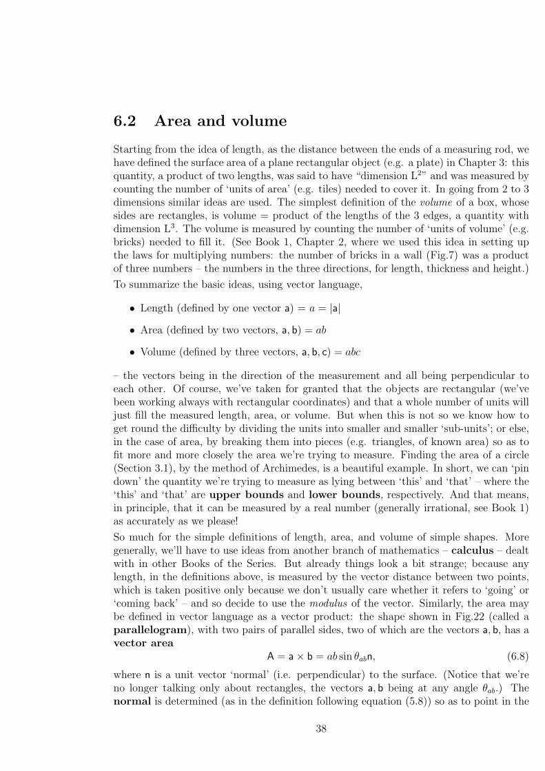
6.2 Area and volume

Starting from the idea of length, as the distance between the ends of a measuring rod, wehave defined the surface area of a plane rectangular object (e.g. a plate) in Chapter 3: thisquantity, a product of two lengths, was said to have “dimension L2” and was measured bycounting the number of ‘units of area’ (e.g. tiles) needed to cover it. In going from 2 to 3dimensions similar ideas are used. The simplest definition of the volume of a box, whosesides are rectangles, is volume = product of the lengths of the 3 edges, a quantity withdimension L3. The volume is measured by counting the number of ‘units of volume’ (e.g.bricks) needed to fill it. (See Book 1, Chapter 2, where we used this idea in setting upthe laws for multiplying numbers: the number of bricks in a wall (Fig.7) was a productof three numbers – the numbers in the three directions, for length, thickness and height.)

To summarize the basic ideas, using vector language,

• Length (defined by one vector a) = a = |a|

• Area (defined by two vectors, a, b) = ab

• Volume (defined by three vectors, a, b, c) = abc

– the vectors being in the direction of the measurement and all being perpendicular toeach other. Of course, we’ve taken for granted that the objects are rectangular (we’vebeen working always with rectangular coordinates) and that a whole number of units willjust fill the measured length, area, or volume. But when this is not so we know how toget round the difficulty by dividing the units into smaller and smaller ‘sub-units’; or else,in the case of area, by breaking them into pieces (e.g. triangles, of known area) so as tofit more and more closely the area we’re trying to measure. Finding the area of a circle(Section 3.1), by the method of Archimedes, is a beautiful example. In short, we can ‘pindown’ the quantity we’re trying to measure as lying between ‘this’ and ‘that’ – where the‘this’ and ‘that’ are upper bounds and lower bounds, respectively. And that means,in principle, that it can be measured by a real number (generally irrational, see Book 1)as accurately as we please!

So much for the simple definitions of length, area, and volume of simple shapes. Moregenerally, we’ll have to use ideas from another branch of mathematics – calculus – dealtwith in other Books of the Series. But already things look a bit strange; because anylength, in the definitions above, is measured by the vector distance between two points,which is taken positive only because we don’t usually care whether it refers to ‘going’ or‘coming back’ – and so decide to use the modulus of the vector. Similarly, the area maybe defined in vector language as a vector product: the shape shown in Fig.22 (called aparallelogram), with two pairs of parallel sides, two of which are the vectors a, b, has avector area

A = a× b = ab sin θabn, (6.8)

where n is a unit vector ‘normal’ (i.e. perpendicular) to the surface. (Notice that we’reno longer talking only about rectangles, the vectors a, b being at any angle θab.) Thenormal is determined (as in the definition following equation (5.8)) so as to point in the

38

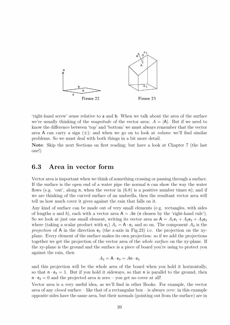
‘right-hand screw’ sense relative to a and b. When we talk about the area of the surfacewe’re usually thinking of the magnitude of the vector area: A = |A|. But if we need toknow the difference between ‘top’ and ‘bottom’ we must always remember that the vectorarea A can carry a sign (±); and when we go on to look at volume we’ll find similarproblems. So we must deal with both things in a bit more detail.

Note: Skip the next Sections on first reading; but have a look at Chapter 7 (the lastone!)

6.3 Area in vector form

Vector area is important when we think of something crossing or passing through a surface.If the surface is the open end of a water pipe the normal n can show the way the waterflows (e.g. ‘out’, along n, when the vector in (6.8) is a positive number times n); and ifwe are thinking of the curved surface of an umbrella, then the resultant vector area willtell us how much cover it gives against the rain that falls on it.

Any kind of surface can be made out of very small elements (e.g. rectangles, with sidesof lengths a and b), each with a vector area A = An (n chosen by the ‘right-hand rule’).So we look at just one small element, writing its vector area as A = A1e1 + A2e2 + A3e3

where (taking a scalar product with e1) A1 = A · e1 and so on. The component A3 is theprojection of A in the direction e3 (the z-axis in Fig.23) i.e. the projection on the xy-plane. Every element of the surface makes its own projection: so if we add the projectionstogether we get the projection of the vector area of the whole surface on the xy-plane. Ifthe xy-plane is the ground and the surface is a piece of board you’re using to protect youagainst the rain, then

A3 = A · e3 = An · e3

and this projection will be the whole area of the board when you hold it horizontally,so that n · e3 = 1. But if you hold it sideways, so that n is parallel to the ground, thenn · e3 = 0 and the projected area is zero – you get no cover at all!

Vector area is a very useful idea, as we’ll find in other Books. For example, the vectorarea of any closed surface – like that of a rectangular box – is always zero: in this exampleopposite sides have the same area, but their normals (pointing out from the surface) are in

39

opposite directions and the vector sum is zero. This is a general result: it means nothingcan flow in or out through a surface that is closed – you’d have to make a hole in it.

Before starting on volume, it’s useful to show how vector area can be written in terms ofcomponents. The vector area of a surface element defined in Fig.22 by the vectors a andb, with a = a1e1 + a2e2 + a3e3, b = b1e1 + b2e2 + b3e3, is A = a × b; and this becomes,remembering that e1 × e2 = e3 = −e2 × e1, etc. and e1 × e1 = 0, etc.,

a× b = (a1e1 + a2e2 + a3e3)× (b1e1 + b2e2 + b3e3)

= (a1b2 − a2b1)e3 − (a1b3 − a3b1)e2

+(a2b3 − a3b2)e1.

To remember things like this we first note that each component depends on two subscripts(e.g. the first on ‘1’ and ‘2’) and is multiplied by −1 if we change their order (e.g.‘1,2’ → ‘2,1’) – it is antisymmetric under interchange of subscripts. There is a specialnotation for such quantities: we write

a1b2 − a2b1 =

∣∣∣∣ a1 a2

b1 b2

∣∣∣∣ , a1b3 − a3b1 =

∣∣∣∣ a1 a3

b1 b3

∣∣∣∣ ,

a2b3 − a3b2 =

∣∣∣∣ a2 a3

b2 b3

∣∣∣∣ ,

so that, from each array on the right, the corresponding component on the left is obtainedas a product of the numbers on the ‘leading diagonal’ (e.g. a1, b2) minus the product ofthose on the ‘second diagonal’ (i.e. b1, a2). With this notation, the vector product abovecan be put in the (re-arranged) form

a× b = e1

∣∣∣∣ a2 a3

b2 b3

∣∣∣∣− e2

∣∣∣∣ a1 a3

b1 b3

∣∣∣∣ + e3

∣∣∣∣ a1 a2

b1 b2

∣∣∣∣ . (6.9)

Each array, with the rule for ‘multiplying it out’ to get a single number, is called adeterminant. We’ll meet determinants in other Books, but for the moment we’re justusing the notation. Similar determinants can be set up, with any number of rows andcolumns, and any of them can be ‘expanded’ in terms of smaller determinants. To showhow useful they can be in helping us to remember very complicated things, let’s look atan expression for the vector product (6.9) as a single determinant with three rows andcolumns: it turns out to be

a× b =

∣∣∣∣∣∣e1 e2 e3

a1 a2 a3

b1 b2 b3

∣∣∣∣∣∣ . (6.10)

To expand this ‘3×3’ determinant in the form (6.9) you take the element in the first rowand the first column (it is e1) and multiply it be the ‘2×2’ determinant that’s left whenyou strike out the first row and column; then you move to the next element in the firstrow (it is e2) and do the same, multiplying it by the determinant that’s left when youstrike out the first row and second column; and then you move to the next element (e3)and multiply it by the determinant that’s left when you strike out the row and column

40

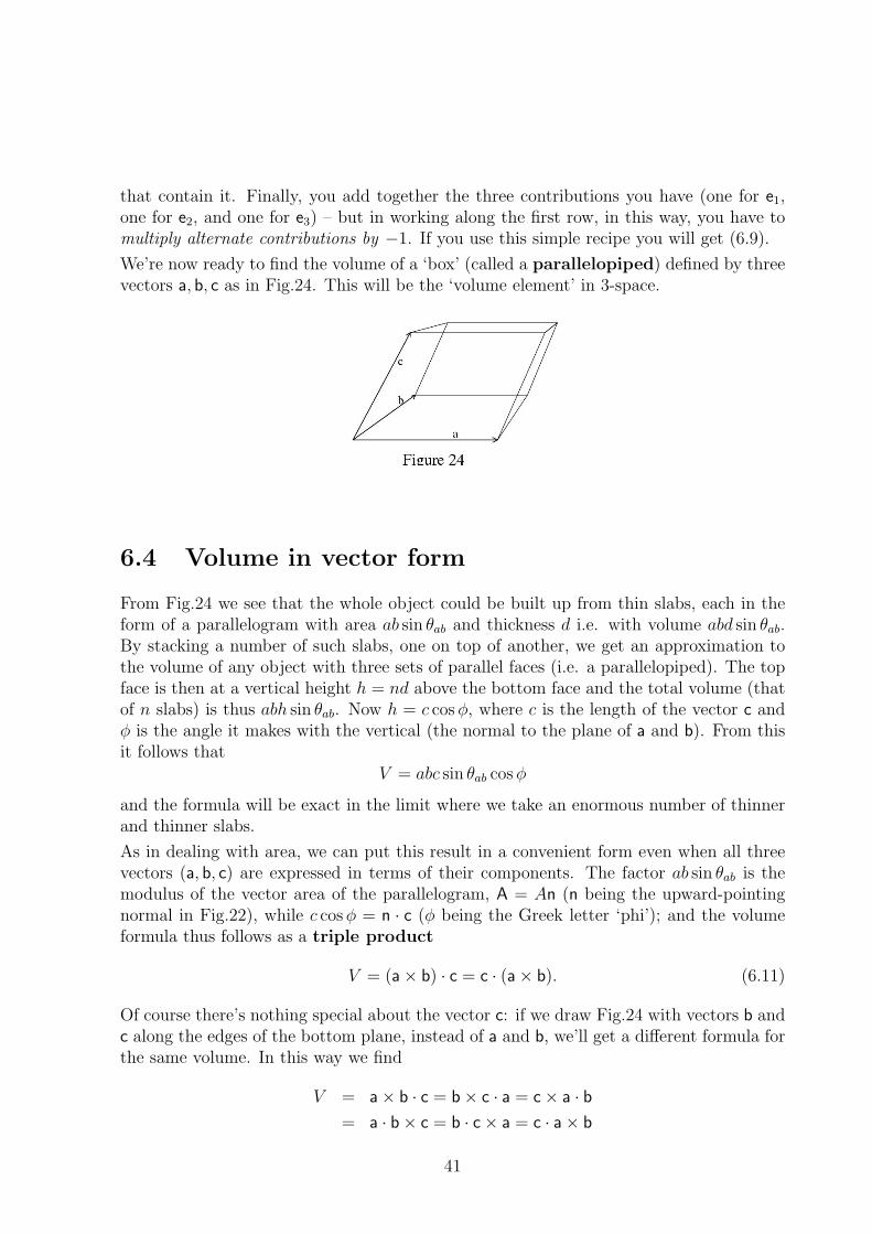
that contain it. Finally, you add together the three contributions you have (one for e1,one for e2, and one for e3) – but in working along the first row, in this way, you have tomultiply alternate contributions by −1. If you use this simple recipe you will get (6.9).

We’re now ready to find the volume of a ‘box’ (called a parallelopiped) defined by threevectors a, b, c as in Fig.24. This will be the ‘volume element’ in 3-space.

6.4 Volume in vector form

From Fig.24 we see that the whole object could be built up from thin slabs, each in theform of a parallelogram with area ab sin θab and thickness d i.e. with volume abd sin θab.By stacking a number of such slabs, one on top of another, we get an approximation tothe volume of any object with three sets of parallel faces (i.e. a parallelopiped). The topface is then at a vertical height h = nd above the bottom face and the total volume (thatof n slabs) is thus abh sin θab. Now h = c cos φ, where c is the length of the vector c andφ is the angle it makes with the vertical (the normal to the plane of a and b). From thisit follows that

V = abc sin θab cos φ

and the formula will be exact in the limit where we take an enormous number of thinnerand thinner slabs.

As in dealing with area, we can put this result in a convenient form even when all threevectors (a, b, c) are expressed in terms of their components. The factor ab sin θab is themodulus of the vector area of the parallelogram, A = An (n being the upward-pointingnormal in Fig.22), while c cos φ = n · c (φ being the Greek letter ‘phi’); and the volumeformula thus follows as a triple product

V = (a× b) · c = c · (a× b). (6.11)

Of course there’s nothing special about the vector c: if we draw Fig.24 with vectors b andc along the edges of the bottom plane, instead of a and b, we’ll get a different formula forthe same volume. In this way we find

V = a× b · c = b× c · a = c× a · b= a · b× c = b · c× a = c · a× b

41

are all expressions for the same volume. The relative positions of the ‘dot’ and the ‘cross’don’t matter, so the triple product is often written as [a b c] and the last results thenbecome

V = [a b c] = [b c a] = [c a b],

where the different forms arise from a cyclic interchange, abc→bca→cab. Note thatwhen the three vectors form a right-handed system, as in Fig.24, the volume V given inthis way is always positive; but if you change this order the sign of the result is reversed.We needn’t worry about this (we usually only want the magnitude of the volume) but wekeep it in mind.

Finally, we express V in terms of the rectangular components of the vectors a, b, c, as wedid in the case of the vector area. Thus, writing V = a ·b× c and using the formula (6.9),but with b, c in place of a, b, we see V can be written as the scalar product of

a = a1e1 + a2e2 + a3e3

and the vector product b× c in the form

e1

∣∣∣∣ b2 b3

c2 c3

∣∣∣∣− e2

∣∣∣∣ b1 b3

c1 c3

∣∣∣∣ + e3

∣∣∣∣ b1 b2

c1 c2

∣∣∣∣ .

From the properties of the Cartesian unit vectors (e1 ·e1 = 1, e1 ·e2 = 0, etc.) this productgives the volume V in the form

a1

∣∣∣∣ b2 b3

c2 c3

∣∣∣∣ − a2

∣∣∣∣ b1 b3

c1 c3

∣∣∣∣ + a3

∣∣∣∣ b1 b2

c1 c2

∣∣∣∣ .

But this is the expanded form of a single ‘3×3’ determinant, as in (6.10); so we can write

V =

∣∣∣∣∣∣a1 a2 a3

b1 b2 b3

c1 c2 c3

∣∣∣∣∣∣ . (6.12)

This is a very general result: the vectors a, b, c can point in any directions and have anylengths we please – we only need to know their 3-space components and we can say atonce what volume element they define.

Exercises

1) Use the transformation equation (6.3), which describes the rotation of all 3-spacevectors around a common axis, to show that the angle between any two vectors, p and q,is unchanged by this rotation.

2) Show that the magnitude of the vector area defined by the two vectors a, b, and thevolume of the parallelopiped defined by three vectors a, b, c, are also invariant under therotation (6.3).

3) Work out the volume of the parallelopiped in the last Exercise, and the vector areas ofits six faces, when the vectors a, b, c are

a = 3e1 + e2, b = e1 + 2e2, c = e1 + e2 + 2e3.

42

Make a drawing in which the vector areas are represented by arrows.

4) Besides the triple product in equation (6.11), which is a scalar quantity, there is alsoa vector triple product. For the three vectors a, b, c this is defined as the vector productof a with b× c: Pabc = a× (b× c). Since Pabc is perpendicular to a and b× c, while thelatter is perpendicular to the plane containing b and c, the triple product must lie in theplane of b, c. Show that

Pabc = (a · c)b− (a · b)c.

(This is quite hard! – and we don’t use it unless we want to prove (7.19), near the end ofthe book. To get the result just given, you should introduce perpendicular unit vectorse1, e2, e3, with e2 parallel to b and e3 in the plane of b, c. You can then put b = be2 andc = c2e2 + c3e3 and also take a = a1e1 + a2e2 + a3e3. On expressing the vector productsin Pabc = a × (b × c) in terms of the components of a, b, c, you should find (noting thatb× c = bc3e2 × e3 = bc3e1) Pabc = a3bc3e2 − a2bc3e3.

This can be re-written - adding and subtracting a term a2bc2e2 -

Pabc = (a2c2 + a3c3)be2 − a2b(c2e2 + c3e3).

The result we set out to prove is the same as this expression when we write the scalarproducts in terms of vector components.)

43

Chapter 7

Some other kinds of space

7.1 Many-dimensional space

So far we’ve been talking mainly about Euclidean spaces of 2 or 3 dimensions – 2-space and3-space. They were vector spaces, containing all the vectors (v) that could be expressed inthe form v = v1e1 + v2e2 (2-space) or v = v1e1 + v2e2 + v3e3 (3-space), where e1, e2, e3 arebasis vectors and the coefficients v1, v2, v3 are algebraic numbers called vector components.To include both cases we can write

v = v1e1 + v2e2 + . . . vnen, (7.1)

where n = 2 for 2-space and n = 3 for 3-space. Remember that every vector had alength (or magnitude) and a direction; and was often represented as an arrow, of givenlength and pointing in the given direction. (Mathematicians call the arrow a “directedline segment”.)

Remember, too, that the components, v1, v2, ..., relate the vector to the basis and giveus a way of labelling any point in space, P, as P(v1, v2, ...). The numbers v1, v2, ... arecomponents of a position vector (often denoted by r) corresponding to the line OPpointing from the origin O to the point P; and they are also called the coordinates of pointP. So far, we have always chosen the basis vectors to be of unit length and perpendicularto one another. In the language of Chapter 6, any two basis vectors (ei, ej) have scalarproducts

ei · ej = 1 when i = j ;

(7.2)

ei · ej = 0 when i 6= j ;

for all values of i, j in the range 1, 2, ..n. This is the choice we started from in Chapter 1,taking it as the “metric axiom” for 2-space (n = 2). And the same choice, but with n = 3,leads to the 3-space considered in Chapter 6. In either case, the properties shown in (7.2)allow us to express the length of any vector in a ‘sum-of-squares’ form. In 3-space, forexample, the square of a velocity vector, |v|2 = v · v, is given by

|v|2 = (v1e1 + v2e2 + v3e3) · (v1e1 + v2e2 + v3e3) = v21 + v2

2 + v23, (7.3)

44

where there are no terms such as v1v2 because e1 · e2 = 0.

The scalar products of the basis vectors are often set out in a square array, like this – e1 · e1 e1 · e2 e1 · e3

e2 · e1 e2 · e2 e2 · e3

e3 · e1 e3 · e2 e3 · e3

=

1 0 00 1 00 0 1

. (7.4)

An array of this kind is called the metric matrix of the space, and all such spaces – inwhich length can be defined as in (7.3) – are called “metric spaces”.

Nothing we’ve said so far depends on n having the value 2 or 3: the simplest generalizationof our ideas about geometry is just to keep everything, but allow n to become bigger thanthree. We then talk about “n-dimensional spaces”. The fact that we can’t imagine them,because we’re so used to living in 3-space, is not important. If we can find a use for them,then we use them!

So let’s put n = 5 and take it as an example of a 5-space. In Book 1, Chapter 6, wetalked about a ‘space’ (though we didn’t call it that) in which there were five categoriesof students in a class of 40. The categories were defined by putting the students intogroups, according to the ranges into which their heights fall. Suppose we measure them

and find the following results:

Heights of students NumbersRange (a): 1m 5cm to 1m 10cm 4 studentsRange (b): 1m 10cm to 1m 15cm 8 studentsRange (c): 1m 15cm to 1m 20cm 13 studentsRange (d): 1m 20cm to 1m 25cm 12 studentsRange (e): 1m 25cm to 1m 30cm 3 students

The numbers in these five categories show the ‘state’ of the class; and if we use a to standfor a student — no matter which one — in category (a), b for one in category (b), and soon, then we can describe the state of the class in symbols as

s = 4a + 8b + 13c + 12d + 3e (7.5)

– which looks surprisingly like a vector! so we’ll call it a state vector.

The students in the five categories can be ‘sorted out’ or selected by introducing selectionoperators (as we did in Book 1). Let’s call them A, B, ... E so that A selects only studentsin group (a), and so on. These operators have (as we discovered) the algebraic properties

AA = A, BB = B, ... EE = E (7.6)

and, for pairs of different operators,

AB = BA = 0, AC = CA = 0, ... DE = ED = 0. (7.7)

And they work on the state vector s as follows:

As = 4a, Bs = 8b, ... Es = 3e,

45

This shows that each selects a part of the class and that putting the results together againwe get the whole class:

(A + B + C + D + E)s = 4a + 8b + ... + 3e = s.

In other words,A + B + C + D + E = 1 (7.8)

– the ‘unit operator’ which leaves any state vector unchanged. Operators with theseproperties form what mathematicians call a “spectral set”: but here we’ve set them upusing a very practical example, rather than snatching them out of the sky – as a realmathematician might do.

But let’s get back to vector spaces. Algebra provides one way of dealing with selection,geometry provides another. When we use the vector (7.5) to stand for the ‘state’ of theschool we’re really thinking of a, b, ... e as ‘basis vectors’ or ‘unit steps’ along five differentaxes. And we can give them any properties we please – supposing, for example, that eachof them is perpendicular to all the others, even though that would be impossible with3-space thinking. The metric matrix will then no longer be (7.4): it will have five ‘1’salong the diagonal and zeros everywhere else. It may all look strange – but who cares?We’re only using a mathematical language and it’s up to us to decide how the symbolsshould behave. Now that we’ve decided, we can think of s in (7.5) as the 5-dimensionalvector formed by taking 4 steps of type a, 8 steps of type b, and so on, and combiningthem by addition (i.e. one after another, as in Fig.19). And the squared length of thevector, with this metric, will be the sum-of-squares of its components.

The selection operators can now be looked at geometrically: As = 4a is simply the projec-tion of the vector s on the axis defined by the unit vector a, while Bs = 8b is its projectionon the b axis. The property AA = A then simply means that projecting twice on a givenaxis can produce nothing more than doing it only once; while BA = 0 means that anyprojection on the a axis will have zero projection on the b axis – that’s why we chose theunit vectors perpendicular (zero scalar products).

Sometimes it’s useful to change this geometrical picture slightly. For example, if we wantto compare two different classes, of different sizes, we’d be more interested in the fractionalnumbers of students in the various groups. In that case we might use a vector

s = (4/40)a + (8/40)b + (13/40)c + (12/40)d + (3/40)e

to show the state of the class, so that the projections along the five axes will representthese fractions directly. But then the ‘pointer’ s, which shows how the students are dividedamong the five groups, would not have very nice properties: if all the students belongedto the same group (a) we’d have s = (40/40)a = a and this would be a unit vector alongthe a axis – but that’s a very special case. Is it possible to choose the vector componentsso that s will always be a unit vector, but will point in different directions according tothe division of students into the five groups?

The components we’ve just tried, namely

(4/40), (8/40), (13/40), (12/40), (3/40),

46

won’t do – because the sum of their squares doesn’t give 1. But the sum of the numbersthemselves does give 1. So why don’t we try

√4/40,

√8/40, ...√

3/4? If we do this, the vector s showing the state of the class will become√4/40 a +

√8/40 b +

√13/40 c +

√12/40 d +

√3/40 e

and the sum of the squares of the components will be exactly 1. So it is possible torepresent the state of the class by a unit vector, pointing out from the origin in a 5-space,in a direction that will show the fractional number of students in each of the 5 categories.

If we want to compare two classes, to see if the heights of the students follow the samepattern, we just ask if the vectors s1 and s2 point in roughly the same direction. If theydo, their scalar product s1 · s2 will have a value close to 1; if the classes are very different(e.g. one of 5-year olds and one of 16-year olds) the scalar product of the vectors will bemuch closer to zero.

This example was about students, divided into groups according to height; but we mighthave been talking about potatoes of different sizes, or about objects produced in a factoryand not all coming out quite right (some too big some too small), and we can use thesame sort of vector description whenever we talk about categories. What’s more, we canchoose the metric in any way that seems useful for what we have in mind — as we’ll seein the next two Sections.

7.2 Special Relativity:

space-time

The starting point for this Book was the idea of distance and how it could be measuredusing a ‘measuring-rod’, whose length (the distance between its ends) was taken as theunit of distance. We also mentioned time, and how it could be measured using a ‘clock’whose pendulum, swinging back and forth, marked out units of time; and also the massof an object, which could be measured using a weighing machine. But so far mass andtime haven’t come into our picture of space: the idea of length alone has allowed us tobuild up the whole of Euclid’s geometry.

Since about 1904, however, all that has changed. Space and time can’t always be sepa-rated: it’s no use giving my address (my ‘coordinates’ in space) if I don’t live there anymore — so perhaps my coordinates should really become x, y, z, t, the last one being thetime at which I am (or was, or will be) there. The four coordinates together define aspace-time point or an event; and when we talk about how things happen, or change,we need all four of them. This is especially true when two people (usually called the“observers”) see the same event: one says it happens at the point x, y, z, t, the othersays it happens at x′, y′, z′, t′. But these numbers depend on the reference frame of theobserver: from what origin in space (where x = y = z = 0) are the distances measured;and when was the clock started (by setting t = 0)? Einstein’s theory of relativity is abouthow the numbers describing the same event, seen by different observers, are related.

47

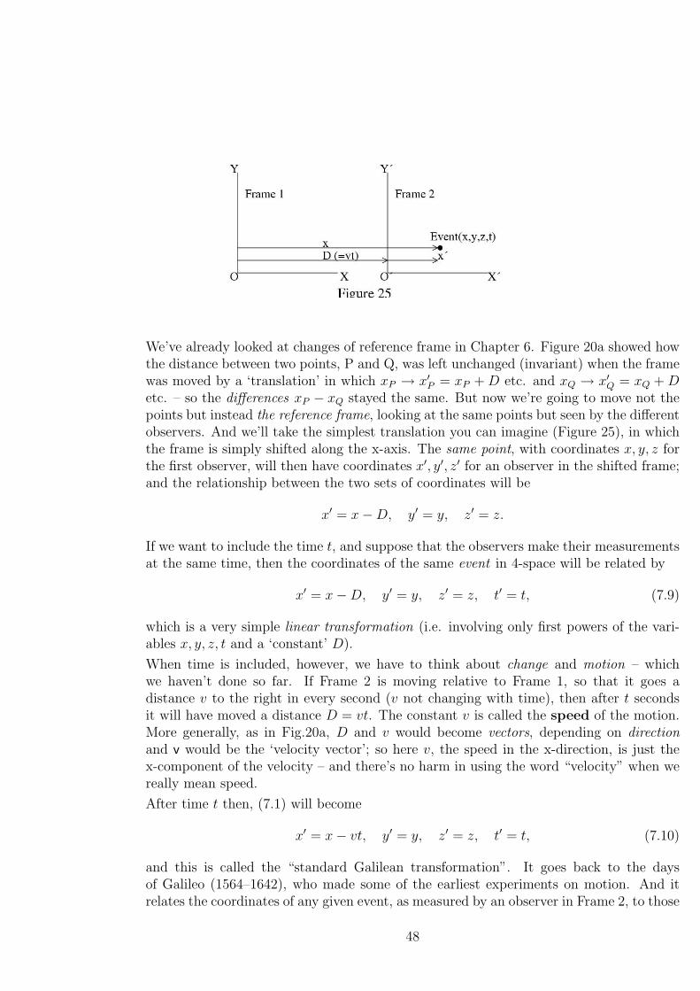
We’ve already looked at changes of reference frame in Chapter 6. Figure 20a showed howthe distance between two points, P and Q, was left unchanged (invariant) when the framewas moved by a ‘translation’ in which xP → x′

P = xP + D etc. and xQ → x′Q = xQ + D

etc. – so the differences xP − xQ stayed the same. But now we’re going to move not thepoints but instead the reference frame, looking at the same points but seen by the differentobservers. And we’ll take the simplest translation you can imagine (Figure 25), in whichthe frame is simply shifted along the x-axis. The same point, with coordinates x, y, z forthe first observer, will then have coordinates x′, y′, z′ for an observer in the shifted frame;and the relationship between the two sets of coordinates will be

x′ = x−D, y′ = y, z′ = z.

If we want to include the time t, and suppose that the observers make their measurementsat the same time, then the coordinates of the same event in 4-space will be related by

x′ = x−D, y′ = y, z′ = z, t′ = t, (7.9)

which is a very simple linear transformation (i.e. involving only first powers of the vari-ables x, y, z, t and a ‘constant’ D).

When time is included, however, we have to think about change and motion – whichwe haven’t done so far. If Frame 2 is moving relative to Frame 1, so that it goes adistance v to the right in every second (v not changing with time), then after t secondsit will have moved a distance D = vt. The constant v is called the speed of the motion.More generally, as in Fig.20a, D and v would become vectors, depending on directionand v would be the ‘velocity vector’; so here v, the speed in the x-direction, is just thex-component of the velocity – and there’s no harm in using the word “velocity” when wereally mean speed.

After time t then, (7.1) will become

x′ = x− vt, y′ = y, z′ = z, t′ = t, (7.10)

and this is called the “standard Galilean transformation”. It goes back to the daysof Galileo (1564–1642), who made some of the earliest experiments on motion. And itrelates the coordinates of any given event, as measured by an observer in Frame 2, to those

48

measured by one in Frame 1 — when Frame 2 moves with constant velocity v, relativeto Frame 1, as in Fig.25. The science of kinematics (from the Greek word ‘kinesis’,meaning movement) deals with length, time, and movement; so now we’re starting tothink about kinematics. In this field the only ‘tools’ we need, in making experiments,are a measuring-rod and a clock; and very often we don’t even need to actually do theexperiments – it’s enough to think about them, making a thought-experiment. We’regoing to make some amazing discoveries, just by thinking about things.

First of all, we’ll suppose our clocks and measuring-rods are perfect. This means that iftwo lengths are found to be equal, then they will stay equal for all times (that’s why weput in the word “perfect”, because a real rod might get bent or broken); and similarlywhen two perfect clocks, both at the origin in some reference frame, show the same times,then they will do so even with a different choice of reference frame. As long as we’retalking about kinematics (not about real objects, which have mass and are affected by‘gravity’ – which we meet in Book 4) that’s all we need.

Suppose you’re in a train, waiting at a station for passengers to get on and off, andanother train is passing. Each train is a reference frame, like the frames in Fig.25, andfrom your window you see people in the other train doing all the usual things – reading thenewspaper, walking about, or even drinking tea: and perhaps you wonder for a momentwhich train is moving? Their train is moving with some velocity v relative to your train,but everything goes on as if it were’nt moving at all. In fact, all movement is relative:your train may not be moving relative to the station – but it is certainly moving (alongwith the whole station, the town, and the earth itself!) relative to the sun and the stars.You actually feel your relative motion only when it changes : if your train suddenly starts,you’ll feel it; if you’re standing you may even fall over. And the people in the other trainwill not notice they are moving with velocity v relative to you, unless v changes : if you seethem falling over, or spilling their tea, you’ll guess that the driver has put the brakes onand the train is slowing down. So there’s something important about a relative velocitybeing constant : observers in two reference frames, moving with constant relative velocity,see things happening in exactly the same way. Albert Einstein (1879-1955) was the firstto see just how important this was – for the whole of Physics. He took it as an axiom,which can be put in the following way:

The laws of physics are exactly the same in any two reference frames in uniformrelative motion (which means moving relative to each other with constantvelocity in a straight line).

We’ll call this Einstein’s Principle of Special Relativity – “special” because objects witha mass, and subject to gravity (the force that makes things fall to the ground), are notyet included in the theory. The ideas of General Relativity, which takes account of massand gravity, are much too difficult for this book, though we mention them briefly in thenext Section. In Relativity Theory, frames “in uniform relative motion” are usually calledinertial frames – but more about that in Book 4, where we begin to talk about mass.

Let’s now go back to equation (7.10) which relates the coordinates of an event, as measuredby observers in the reference frames of Fig.25. The observer in Frame 1, finds values

49

x, y, z, t, while the observer in Frame 2 finds values x′, y′, z′, t′ relative to his axes; both ofthem using the same standard unit of length and both having set their standard clocksto t = t′ = 0 at the start of the experiment when, we suppose, the origin of Frame 2 isjust on top of the origin of Frame 1. The distance in space to the event, call it s, is thesame for both observers:

s2 = x2 + y2 + z2 = x′2 + y′2 + z′2

and both believe t = t′, as they set their clocks to agree at the start (when O′ was passingO). The invariance of these quantities, in passing from one reference frame to the otheris what leads to the ‘transformation equations’ (7.10), which now become

x′ = x− vt,

y′ = y,

z′ = z,

t′ = t. (7.11)

But this transformation is a bit too special: it keeps s2 and t the same for both observers,but keeps them separately invariant – s2 in 3-space, t in a 1-space. However, we agreed thattime should be treated as just another coordinate. Is there a more general transformation,that will allow space and time coordinates to get mixed up? When this can happen, we’llbe talking about a 4-space!

To see that such a transformation can be found, let’s think of another simple event. Wefire a gun, at the origin, at time t = t′ = 0 just as O′ is passing O. The noise travels outfrom the gun, in all directions, with some constant speed which we can call c. After timet it will have reached all the points at a distance r = ct from the origin O. These will lieon a surface of radius r = ct (a sphere) such that

r2 = c2t2 = x2 + y2 + z2.

If we could assume that an observer in Frame 2 (along with his friends – all with standardclocks – placed at points where the noise arrived) all observed the same sphere of noisearrivals, then we’d suppose that

s2 = c2t2 − x2 − y2 − z2 = c2t′2 − x′2 − y′2 − z′2 (7.12)

was another invariant. We call it the squared interval (not just ‘distance’) and it dependson all four coordinates. Notice that (7.12) defines a 4-space metric that’s a bit strange:it has a matrix like that in (7.4) but with three diagonal elements the same, the fourthhaving opposite sign (e.g. three −1s and one +1). But, after all, time (we’ve given it a‘time coordinate’ ct) and space (with coordinates x, y, z) are different – and this showsup in the sign difference.

Of course, a ‘thought experiment’ like this would be difficult to do; and we don’t know ifit has any relationship to the real world. But it does suggest something we can try.

50

Let’s suppose then, that in Einstein’s 4-space the space and time coordinates of eventsobserved from frames in uniform relative motion (Fig.25) are related so that (7.12) issatisfied. The big question is now: What is this relationship? And to get the answer wecan argue as follows.

The new invariant contains a new constant (c), also a velocity, like the v in (7.11); andso v/c must be a pure number, which will go to zero if the constant c is big enough, or ifv is small enough. Let’s now define a number, usually called γv (Greek ‘gamma’, with asubscript to show it depends on the relative velocity v):

γv =1√

(1− v2/c2). (7.13)

Notice that we’ve used the squares of the velocities in the denominator, because changingthe direction of the x-axis will change the sign of a velocity – and we don’t expect itwill matter whether the axis points to the right or the left. Also, when v is small thedenominator in (7.13) will go towards 1 – and so will γv. So if the new transformationequations depend on γv they will fall back into the Galilean transformation when the tworeference frames are hardly moving– just as we’d expect.

Let’s now try, instead of the first three equations in (7.11),

x′ = γv(x− vt), y′ = y, z′ = z.

And instead of taking time to be universal, the same for both observers, let’s try somethinga bit like the first equation above. If we put

t′ = γv(t− ?× x),

where ‘?’ stands for something we don’t yet know, then we can substitute the valuesof x′, y′, z′, t′ (given in the last four equations) into the right-hand side of (7.12); andcomparing the two sides will tell us what to choose for the ‘?’. The only terms thatcontain t alone (not t2) are c2γ2

v × (−2xt×?) and 2γ2vxvt. There’s nothing to balance

these terms on the left-hand side of (7.12), so the equality tells us that their sum mustbe zero and this fixes the ‘?’ To get zero we must choose ?= v/c2 and so we must take

t′ = γv

(t− v

c2x)

.

What we have shown is that the supposed invariance of the ‘metric form’ c2t2−x2−y2−z2

requires that the Galilean transformation equations be changed, becoming

x′ = γv(x− vt),

y′ = y,

z′ = z,

t′ = γv

(t− v

c2x)

. (7.14)

51

These are the equations of the Lorentz transformation, named after the Dutch math-ematician and physicist Lorentz (1857–1928), who first got them, but never guessed howthey would change the world! That was left to Einstein, who found them again and madethem a cornerstone of his relativity theory.

Nowadays we’re always hearing about mass and energy (who hasn’t ever seen Einstein’sfamous equation E = mc2?), atomic power, atomic bombs, space travel, and the strangethings that happen in the universe. But let’s stop for a minute! We haven’t even got asfar as physics: that will have to wait for other Books (beginning in Book 4). This Sectionis just a start, in which we’re beginning to use some of the things we already know aboutnumber and space. Before this we didn’t even include time, and we still haven’t reallythought about mass. So it’s amazing that we can get so far just by thinking about things.Before stopping we’ll connect briefly with what we call ‘reality’ – a few questions and afew conclusions.

The first question is What is the meaning of the constant c? and the second is How bigis it? – and does it correspond to anything we can measure? In fact, there is somethingthat travels through empty space with the velocity c: it is light, which we all know goesextremely fast – if you switch a light on it seems to fill the whole room in no time atall! Physics tells us what light is and gives us ways of finding how fast it travels: if theswitched-on light starts from the origin, then it reaches a point with (space) coordinatesx, y, z after a time t given by t = (distance/velocity) =

√x2 + y2 + z2/c, where c can

be calculated in terms of quantities we can measure in the laboratory. And its valueis almost exactly 300 million metres every second (3×108m s−1), so in everyday life weneedn’t worry about using the Galilean equations (7.10). The other big question is Howdid we get so far without knowing any physics? The answer is not at all easy, but roughlyspeaking it’s because we left out mass and gravity, and electric charges, and most of thethings that go into physics – thinking only of kinematics (length, time, and motion) –except when we supposed that all the ‘physics’ was the same for “two observers in uniformrelative motion”. We didn’t need all the details: the Lorentz transformation follows, as wesaw, from kinematical principles. We’re just lucky to find that physics supplies a ‘natural’method of getting the value of the constant c.

What about conclusions? The first one is that there’s a natural limit to the speed withwhich anything can move – even an observer in a spacecraft – and this limit is v = c. Forthen γv in (7.13) would become infinite; and for v > c it would become imaginary. Allthe quantities we measure and relate must be real ; and finite, so the only velocities wecan consider must be less than c.

There are many more amazing conclusions. We’ll just mention two: if an observer inFrame 1 looks at an object in Frame 2, he’ll be surprised to find that it has shrunk in thedirection of motion; and that a clock in Frame 2 is going slow!

The Lorentz contraction

Suppose we have a measuring-rod of length l0, lying along the x-axis and not movingrelative to Frame 2; and call its ends A and B. It will be moving relative to us, in Frame1, with velocity v. But to an observer in Frame 2 it will be at rest and will have a proper

52

length, also called rest length,l0 = x′

B − x′A, (7.15)

not depending on what time his clock shows.

Looking at the rod from our reference frame (Frame 1), the length of the rod at time ton our clock will be

l = xB(t)− xA(t). (7.16)

But we know from (7.14) how the coordinates measured in the two frames must be related:

x′A = γv(xA − vt), x′

B = γv(xB − vt).

It follows that, using (7.15),

l0 = x′B − x′

A = γv(xB − xA) = γvl,

where l, given in (7.16), is the length of the rod according to us. Thus,

l = l0/γv. (7.17)

In other words, the measured length of the rod when it’s moving away from us withvelocity v, will be less than the rest length – as measured in a frame where it is notmoving. This effect is called the Lorentz contraction. It is very small for speeds whichare tiny compared with c (≈ 300 thousand kilometres/second): so we never notice it ineveryday life. But it is important in physics – and accurate measurements are in perfectagreement with the predictions.

Time dilation

Another remarkable conclusion follows just as easily. A clock moving away from us willregister intervals of time different from those shown by a clock at rest in our referenceframe: times get longer – an effect called time dilation.

Remember, we measured the times t, t′ from the moment when the clock at the origin inFrame 2 passes that in Frame 1, setting t′ = t = 0. The clock at the origin in Frame2 will be at the point with x′ = 0 but relative to Frame 2 its position at time t will bex = vt. Now according to the last equation in (7.14) the times shown, for the same event(as noted by two different observers), must be related by

t′ = γv

(t− v

c2x)

= γvt

(1− v2

c2

)= γvt/γ

2v = t/γv,

where we’ve put in the value x = vt, for the moving clock, and used the definition of γv

in (7.13). Thus,t = γvt

′. (7.18)

In other words, all times measured in the moving system (Frame 2) must be multiplied byγv to get the times measured on our clock in Frame 1. Now the time taken for somethingto happen – the time between two events, A and B say, at a given position in space – willbe T0 = t′B−t′A for an observer moving with his clock (Frame 2): he will call it his “proper

53

time”. And this leads to some very strange effects: for instance, if Frame 2 comes back tothe origin O in Fig.25, after travelling all the way round the world, the Frame 1 observer(who stayed at home with his clock) will note that the journey took time T = γvT0 – whichis longer than the time (T0) noted by the traveller. Who is right? Both are: each hashis own ‘proper time’ and we shouldn’t be surprised if they don’t agree. The differencesare normally almost too small to measure: but, by using extremely accurate (‘atomic’)clocks and taking them round the world on ordinary commercial aircraft, they have beenmeasured and are in rough agreement with the formula. More accurate experiments reallydo confirm (7.18).

7.3 Curved spaces: General

Relativity

In Section 1.1 we said that “space itself is very slightly ‘bent’, especially near very heavythings like the sun and the stars, so that Euclid’s ideas are never perfectly correct ... ”One of Einstein’s most brilliant ideas, which he developed during the years 1905–1915,was that the mass of a heavy object produced a local ‘curvature’ in the space around it:this led him from the theory of Special Relativity to that of General Relativity, in whichmass and its effects are included. As we haven’t yet done any Physics we can’t even beginto talk about General Relativity. But we are ready to think about ‘curved space’ andwhat it means.

In Special Relativity the 4-space metric (three space coordinates and one more for time)was very similar to that for ordinary Euclidean 3-space (Section 5.2): the square of theinterval (‘distance’) between two events (‘points’ in space-time) still had a ‘sum-of-squares’form, apart from the ± signs attached to the 4 terms; and it had the same form howeverbig the interval. A space like that is called ‘pseudo-Euclidean’.

In General Relativity, the metric form is no longer so simple; and it’s no longer the samefor all points in space – it can depend on where you are. To get an idea of what this meanswe’ll use the example from Section 1.1: the surface of the earth is a curved space, thoughit’s only a 2-space and it’s a bit special because the curvature is the same at all points –how much it’s bent depends only on the radius of the earth. Of course, the mathematicsof curved surfaces is important for making maps. And it was important in the ancientworld because the astronomers at that time believed the sun and the moon moved aroundthe earth on spherical surfaces. The Hindus and Arabs invented many arithmetic rulesfor making calculations of their positions, but the rules were not turned into algebraicformulas until about the 13th century. The theory that followed tells us how to calculatelengths and angles for lines which are ‘as straight as you can make them’ on a sphericalsurface. Such a line follows the shortest path between two points, A and B, on the surfaceand is called a geodesic (from the Greek words for ‘earth’ and ‘measurement’). If a shipsails from point A on the earth’s surface, to point B, always keeping the same direction,and does the same in going from B to a third point C, then the three-sided path ABCis called a spherical triangle. The geometry of such paths was studied by mariners for

54

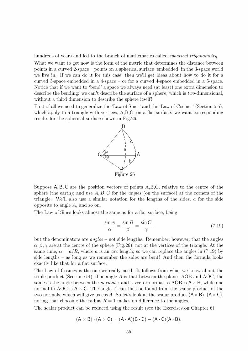
hundreds of years and led to the branch of mathematics called spherical trigonometry.

What we want to get now is the form of the metric that determines the distance betweenpoints in a curved 2-space – points on a spherical surface ‘embedded’ in the 3-space worldwe live in. If we can do it for this case, then we’ll get ideas about how to do it for acurved 3-space embedded in a 4-space – or for a curved 4-space embedded in a 5-space.Notice that if we want to ‘bend’ a space we always need (at least) one extra dimension todescribe the bending: we can’t describe the surface of a sphere, which is two-dimensional,without a third dimension to describe the sphere itself!

First of all we need to generalize the ‘Law of Sines’ and the ‘Law of Cosines’ (Section 5.5),which apply to a triangle with vertices, A,B,C, on a flat surface: we want correspondingresults for the spherical surface shown in Fig.26.

O Aa

��

��

���

B

bQ

QQ

QQQC

c

αγ

β

Figure 26

Suppose A, B, C are the position vectors of points A,B,C, relative to the centre of thesphere (the earth); and use A, B, C for the angles (on the surface) at the corners of thetriangle. We’ll also use a similar notation for the lengths of the sides, a for the sideopposite to angle A, and so on.

The Law of Sines looks almost the same as for a flat surface, being

sin A

α=

sin B

β=

sin C

γ, (7.19)

but the denominators are angles – not side lengths. Remember, however, that the anglesα, β, γ are at the centre of the sphere (Fig.26), not at the vertices of the triangle. At thesame time, α = a/R, where a is an arc length; so we can replace the angles in (7.19) byside lengths – as long as we remember the sides are bent! And then the formula looksexactly like that for a flat surface.

The Law of Cosines is the one we really need. It follows from what we know about thetriple product (Section 6.4). The angle A is that between the planes AOB and AOC, thesame as the angle between the normals : and a vector normal to AOB is A×B, while onenormal to AOC is A× C. The angle A can thus be found from the scalar product of thetwo normals, which will give us cos A. So let’s look at the scalar product (A×B) · (A×C),noting that choosing the radius R = 1 makes no difference to the angles.

The scalar product can be reduced using the result (see the Exercises on Chapter 6)

(A× B) · (A× C) = (A · A)(B · C)− (A · C)(A · B).

55

For a sphere of unit radius,

B · C = cos α, C · A = cos β, A · B = cos γ.

Also A ·B is a vector of length sin γ, normal to the plane AOB and pointing inwards (i.e.onthe C-side); while A · C is of length sin β, normal to plane AOC but pointing outwards.

On putting these values into the expression above, we find

(A× B) · (A× C) = sin β sin γ cos A = cos α− cos β cos γ.

There are two other relations of similar form, obtained by starting from angle B and angleC (instead of A). They are all collected in the Law of Cosines for a spherical triangle:

cos α = cos β cos γ + sin β sin γ cos A,

cos β = cos γ cos α + sin γ sin α cos B, (7.20)

cos γ = cos α cos β + sin α sin β cos C,

for the cosines. The angles α, β, γ (radian measure) are related to the arc lengthsBC, CA, AB on the spherical surface: for example, putting BC = a, the angle α isgiven by α = a/R, where R is the radius of the sphere.

Now think of A as an ‘origin of coordinates’ on the surface and take the outgoing arcs,AB and AC, as axes, choosing the angle between them as A = π/2. On putting cos A = 0,the first line in (7.20) tells us that

cos α = cos β cos γ (7.21)

and this gives us all we need. For points near to A, it’s enough to use the first few termsof the cosine series (Chapter 4) and to write the last equation as

1− a2

2R2+

a4

24R4.. =(

1− b2

2R2+

b4

24R4..

) (1− c2

2R2+

c4

24R4..

).

If we multiply everything by 2R2 and compare the terms of second degree on the twosides of the = sign, the result is a first approximation:

a2 ≈ b2 + c2, (7.22)

The squared length of the arc BC has Euclidean form: it is a sum of squares of distancesalong the other two arcs – in accordance with the metric axiom in Section 1.2 – just asit would be for a flat surface. But the metric is only locally Euclidean: more accurately,there are ‘correction terms’

−(1/12R2)a2, and − (1/12R2)(b4 + c4)− b2c2/R2,

which must be added on the left and on the right, respectively, of equation (7.22).

56

Of course, when the radius of curvature R, is infinitely large the 2-space becomes flat(zero curvature); but in General Relativity even a very small curvature of 4-dimensionalspace-time is enough to account for many properties of the universe. Without Physics,which we’ll start with in Book 4, it’s not possible to go any further: but without thegenius of Einstein and others like him it would never have been possible to get this far.

Exercises

1) When we use the vector (7.5) to stand for the ‘state’ of a class (how big are the studentsin it) we’re using a, b, ... e as ‘basis vectors’. The components we used, namely

4

40,

8

40.13

40.12

40,

3

40

(being the fractional numbers of students in the five height ranges) didn’t give a unitvector – because the sum of their squares doesn’t give 1.

Show that by using the square roots of the numbers as components you will always get aunit vector. So it is possible to represent the state of the class by a unit vector, pointingout from the origin in a 5-space in a direction that will show the fractional number ofstudents in each of the 5 categories.

2) Suppose you want to compare two classes, to see if the heights of the students followthe same pattern. Prepare vectors s1 and s2, like that in Exercise 1 but for two differentclasses (e.g. 20 15-year old girls and 18 14-year old boys). Is the pattern of heights similaror not?

(You can either measure or just guess the heights. The patterns will be similar if thevectors point in roughly the same direction. If they do, their scalar product s1 · s2 willhave a value close to 1. For two very different classes (e.g. one of 5-year olds and one of16-year olds) the scalar product of the vectors will be much closer to zero.)

57

Looking back –

You started this book knowing only about numbers and how to work with them, usingthe methods of algebra. Now you’ve learnt how to measure the quantities you meet inspace (distances, area, volume), each one being a number of units. And you’ve seen thatthese ideas give you a new starting point for geometry, different from the one used byEuclid, and lead you directly to modern forms of geometry. Again, you’ve passed manymilestones on the way:

• Euclid started from a set of axioms, the most famous being that two parallelstraight lines never meet, and used them to build up the whole of geometry: inChapter 1 you started from different axioms – a distance axiom and a metricaxiom – which both follow from experiment.

• Two straight lines, with one point in common, define a plane; the metric axiomgave you a way of testing to see if the two lines are perpendicular; and then youwere able to define two parallel straight lines – giving you a new way of looking atEuclid’s axiom. Using sets of perpendicular and parallel straight lines you could findnumbers (x, y), the coordinates, that define any point in the plane. Any straightline in the plane was then described by a simple equation; and so was a circle.

• In Chapter 3 you learnt how to calculate the area of a triangle and of a circle andto evaluate π (‘pi’) by the method of Archimedes. You studied angles and foundsome of the key results about the angles between straight lines that cross.

• Chapter 4 reminded you of some of the things you’d learnt in Book 1, all neededin the study of rotations. You learnt about the exponential function, ex, de-fined as a series, and its properties; and found its connection with angle and the‘trigonometric’ functions.

• In talking about 3-space, the first thing to do was to set up axes and decide howto label every point with three coordinates; after that everything looked much thesame as in 2-space. But it’s not easy to picture things in 3-space and it’s better touse vector algebra. For any pair of vectors we found two new ‘products’ – a scalarproduct (just a number) and a vector product (a new vector), both dependingon the lengths of the vectors and the angle between them. Examples and Exercisesshowed how useful they could be in 3-space geometry.

• Chapter 6 was quite hard! But the ideas underneath can be understood easily:lengths, areas and volumes are all unchanged if you move something through space– making a ‘transformation’. This fact was often used by Euclid (usually in 2-space)in proving theorems about areas; but by the end of the Chapter you have all the‘tools’ for doing things much more generally, as we do them today.

• To end the book (Chapter 7) you took a look at the next big generalization – tospaces of n dimensions, where n is any integer. Of course, you couldn’t imagine

58

them: but the algebra was the same, for any value of n. So you were able to inventnew spaces, depending on what you wanted to use them for. One such space wasinvented by Einstein, just a hundred years ago, to bring time into the description ofspace – counting t as a fourth coordinate, similar to x, y, z. And you got a glimpse ofsome of the amazing things that came out as a result, things that could be checkedby experiment and were found to be true.

Before closing this book, stop for a minute and think about what you’ve done.Perhaps you started studying science with Book 1 (two years ago? three orfour years ago?) and now you’re at the end of Book 2. You started from almostnothing; and after working through about 150 pages you can understand thingsthat took people thousands of years to discover, some of the great creationsof the human mind – of the Scientific Mind.

59

Index

Antisymmetric,changing sign, 50

Angles, 18-20alternant, 20-21complementary, 20-21

Area 15-19, 47-50Array 50Axioms (first principles), 3

of geometry, 3-5Axis, axes, 4

of coordinates, 4, 7

Basis vectors 36Bounds (upper, lower) 48

Circlearea of, 20circumference of, 20equation of, 13

Components 37, 54Congruence, congruent 47Converse (of theorem) 32Coordinates 9, 34Cosine (see Trigonometric functions)Cyclic interchange 52

Determinant 50-51Differentials, 10, 34Dimensions (physical) 16Direction cosines 39Distance, 1-4

Exponential function 26

Geodesic 66Geometry (science of space) 2

analytical, 5Euclidean, 2-4non-Euclidean, 66

Identity operator 19, 23Image 45Intercept 11Intersect (cross at a point) 4Invariance, invariant 16, 44, 47Inverse operator 19, 23

Kinematics 59

Law of combination 19, 23Law of Sines 40, 67Law of Cosines 40, 68

Metricaxiom, 4form, 10, 34matrix, 55curved space, 69

Modulus (of a vector) 38

Normal (to plane) 38, 40, 48

Origin (of coordinates) 4, 37

Parallel (definition), 8lines, 8, 32planes, 33

Parallelogram 48Parallelopiped 51Perimeter 16Period, periodic, 29Perpendicular (property of axes), 4Perpendicular (from point to plane), 30-32Plane, 4Polygon 17Position vector 37Projection 34, 49

Radian 20

60

Relativity theorygeneral 66-69special 57-65

Rectangle 9Rectangular box 6Rectangular (Cartesian)

coordinates,in 2-space, 9in 3-space, 34

Reference frame 35, 58Right-angle, right-angled 4Rotation (of object) 45Rotation (of vector) 24Rotation operator 23-24

Scalar product 38triple product, 52

Series 25-28Simultaneous equations 12Sine (see Trigonometric functions)Slope (of line) 11Space-time 58Sphere (equation of) 35, 42Straight line,

as shortest path,1-3Subspace, 34

Tangent (Trigonometric functions) 18Tangent (as slope of line) 11Tangent (to a sphere) 42Theorem 5Transformation 16, 44-47

Galilean, 59Lorentz, 63

Translation 45Trigonometric functions 18

series for, 28-29Trigonometry 3

Vector 23-24, 54-57Vectors in 3-space 36-39Vector area 48Vector product 38Vertex 17Volume 51-53

61