space plasma physics (2012) t. wiegelmann
TRANSCRIPT

4/18/2012
1
Space Plasma Physics Thomas Wiegelmann, 2012
1. Basic Plasma Physics concepts
2. Overview about solar system plasmas
3. Single particle motion, Test particle model
4. Statistic description of plasma, BBGKY- Hierarchy and kinetic equations
5. Fluid models, Magneto-Hydro-Dynamics
6. Magneto-Hydro-Statics
7. Stationary MHD and Sequences of Equilibria
Plasma Models
Physical Processes
8. Plasma Waves, instabilities and shocks
9. Magnetic Reconnection
Applications
10. Planetary Magnetospheres
11. Solar activity
12. Transport Processes in Plasmas
Space Plasma Physics
Used Material • Lecture notes from Eckart Marsch 2007
• Baumjohann&Treumann: Basic Space Plasma Physics
• Schindler: Physics of space plasma activity
• Priest: Solar MHD
• Kulsrud: Plasma Physics for Astrophysics
• Krall & Trivelpiece: Principles of Plasma Physics
• Chen: Introduction to plasma physics and controlled fusion
• Balescu: Plasma Transport (3 volumes)
• Spatschek: Theoretische Plasmaphysik
• Wikipedia, Google and YouTube
William Crookes (1832-1919)
called ionized matter in a gas
discharge (Crookes-tube, photo)
ず4th state of matterさ (Phil. Trans 1879)
What is plasma?
Levi Tonks (1897-1971) and
Irving Langmuir (1881-
1957, photo) first used the
term ずplasmaさ for a
collection of charged
particles (Phys. Rev. 1929)
In plasma physics we
study ionized gases
under the influence of
electro-magnetic fields.
Source: Wikipedia
Industrial Plasmas
Neon-lights, Fluorescent
lamps,Plasma globes
Electric Arcs
Nuclear Fusion,
here a Tokamak
Semi conducter
device fabrication
St. Eノマラけゲ Fire
Natural Plasmas on Earth
Ball lightning
Lightning
Aurorae Source: Wikipedia

4/18/2012
2
Accretion discs Space Plasmas
Interior and atmosphere of Sun+Stars
Planetary magnetospheres, solar wind, inter-planetary medium Source: Wikipedia
Source: Wikipedia
Comparison: Gas and Plasma
Plasmas studied in this lecture
• Non-relativistic particle velocities v<<c
• Spatial and temporal scales are large compared to
Planck length (1.6 10-35 m) and time (5.4 10-44 s)
More precise: Any action variables like
(momentum x spatial dimension, Energy x time) are
large compared to Planck constant (h= 6.6 10-34 Js)
Classic plasma, no quantum-mechanic effects.
• Plasmas violating these conditions
(Quark-Gluon Plasma, relativistic plasma) are active
areas of research, but outside the scope of this
introductory course.
What is a plasma?
• A fully or partly ionized gas.
• Collective interaction of charged particles
is more important than particle-particle
collisions.
• Charged particles move under the influence of
electro-magnetic fields (Lorentz-force)
• Charged particles cause electric fields,
moving charged particles cause electric currents
and thereby magnetic fields (Maxwell equations).

4/18/2012
3
What is a plasma?
• In principle we can study a plasma by
solving the Lorentz-force and Maxwell-
equations selfconsistently.
• With typical 10^20-10^50 particles in space
plasmas this is not possible.
(Using some 10^9 or more particles with this
approach is possible on modern computers)
=> Plasma models
Plasma models - Test particles:
Study motion of individual charged particles under
the influence of external electro-magnetic (EM) fields
- Kinetic models:
Statistic description of location and velocity of
particles and their interaction + EM-fields.
(Vlasov-equation, Fokker-Planck eq.)
- Fluid models:
Study macroscopic quantities like density, pressure,
flow-velocity etc. + EM-fields (MHD + multifluid models)
- Hybrid Models: Combine kinetic + fluid models
Maxwell equations for electro-magnetic fields
The motion of charged particles in space is strongly influenced by the self-
generated electromagnetic fields, which evolve according to AマヮWヴWけゲ and
F;ヴ;S;┞けゲ (induction) laws (in this lecture we use the SI-system):
where 0 and 0 are the vacuum dielectric constant and free-space
magnetic permeability, respectively. The charge density is and the current
density j. The electric field obeys Gauss law and the magnetic field is always
free of divergence, i.e. we have:
Electromagnetic forces
The motion of charged particles in space is
determined by the electrostatic Coulomb force
and magnetic Lorentz force:
where q is the charge and v the velocity of any charged
particle. If we deal with electrons and various ionic species
(index, s), the charge and current densities are obtained,
respectively, by summation over all kinds of species as
follows:
which together obey the continuity equation,
because the number of charges is conserved, i.e. we
have:
A plasma is quasi-neutral
• On large scales the positive (ions) and
negative charges cancel each other.
• On small scales charge separations occur.
Can we estimate these scales?
=> Do calculations on blackboard.
Electro-static effects Debye-length
Remark: Some text-books drop the
factor sqrt(3/2)~1.2

4/18/2012
4
Debye-length
• Electric potential for a charge in vacuum:
• Electric potential in a plasma:
=> Debye shielding
Debye shielding
Source: Chen, Wikipedia
Debye shielding
Source: Technik-Lexikon
Plasma Oscillations
• How does a charged particle (say an electron)
move in a non-magneticed plasma?
• Solve electrostatic Maxwell equation
selfconsistently with equation of motion,
here for the Coulomb force
• => Do calculations on blackboard.
Plasma Oscillations
• Plasma frequency
• Electron plasma frequency
is often used to specify the electron density of a plasma. How? => Dispersion relation of EM-waves See lecture of plasma waves.
Plasma parameter
• The plasma paramter g indicates the
number of particles in a Debye sphere.
• Plasma approximation: g << 1.
• For effective Debye shielding and
statistical significants the number of
particles in a Debye sphere must be high.
4/18/2012
5
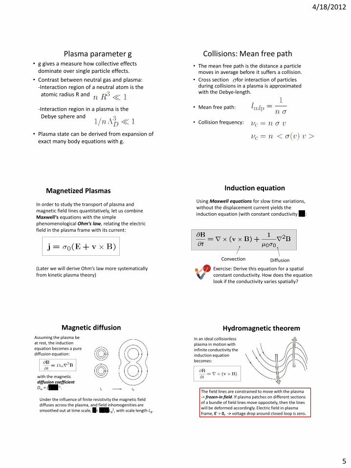
Plasma parameter g • g gives a measure how collective effects
dominate over single particle effects.
• Contrast between neutral gas and plasma:
-Interaction region of a neutral atom is the
atomic radius R and
-Interaction region in a plasma is the
Debye sphere and
• Plasma state can be derived from expansion of
exact many body equations with g.
Collisions: Mean free path
• The mean free path is the distance a particle moves in average before it suffers a collision.
• Cross section for interaction of particles during collisions in a plasma is approximated with the Debye-length.
• Mean free path:
• Collision frequency:
Magnetized Plasmas
In order to study the transport of plasma and
magnetic field lines quantitatively, let us combine
M;┝┘Wノノけゲ equations with the simple
phenomenological Oエマけゲ law, relating the electric
field in the plasma frame with its current:
(Later we will derive Oエマけゲ law more systematically
from kinetic plasma theory)
Induction equation
Using Maxwell equations for slow time variations,
without the displacement current yields the
induction equation (with constant conductivity 0):
Convection Diffusion
Exercise: Derive this equation for a spatial
constant conductivity. How does the equation
look if the conductivity varies spatially?
Magnetic diffusion
Assuming the plasma be
at rest, the induction
equation becomes a pure
diffusion equation:
with the magnetic
diffusion coefficient
Dm = ( 0 0)-1.
Under the influence of finite resistivity the magnetic field
diffuses across the plasma, and field inhomogenities are
smoothed out at time scale, d= 0 0 LB2, with scale length LB.
Hydromagnetic theorem
In an ideal collisionless
plasma in motion with
infinite conductivity the
induction equation
becomes:
The field lines are constrained to move with the plasma
-> frozen-in field. If plasma patches on different sections
of a bundle of field lines move oppositely, then the lines
will be deformed accordingly. Electric field in plasma
frame, E' = 0, -> voltage drop around closed loop is zero.
4/18/2012
6
Assuming the plasma streams at bulk speed V, then
the induction equation can be written in simple
dimensional form as:
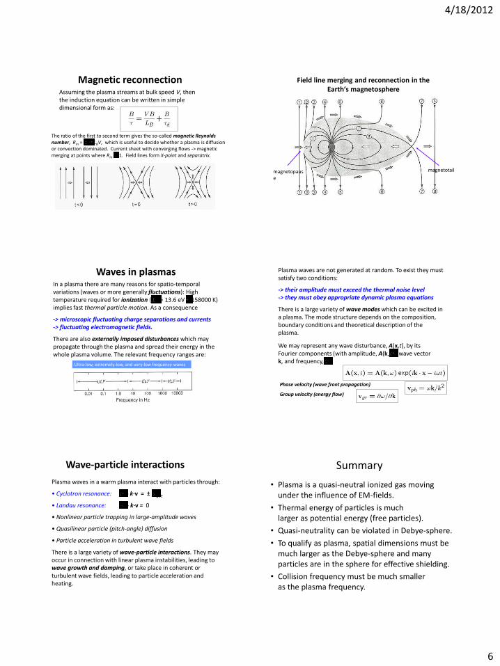
Magnetic reconnection
The ratio of the first to second term gives the so-called magnetic Reynolds
number, Rm = 0 0LBV, which is useful to decide whether a plasma is diffusion
or convection dominated. Current sheet with converging flows -> magnetic
merging at points where Rm 1. Field lines form X-point and separatrix.
Field line merging and reconnection in the
E;ヴデエけゲ マ;ェミWデラゲヮエWヴW
magnetopaus
e
magnetotail
Waves in plasmas In a plasma there are many reasons for spatio-temporal
variations (waves or more generally fluctuations): High
temperature required for ionization ( H = 13.6 eV 158000 K)
implies fast thermal particle motion. As a consequence
-> microscopic fluctuating charge separations and currents
-> fluctuating electromagnetic fields.
There are also externally imposed disturbances which may
propagate through the plasma and spread their energy in the
whole plasma volume. The relevant frequency ranges are:
Ultra-low, extremely-low, and very-low frequency waves
Plasma waves are not generated at random. To exist they must
satisfy two conditions:
-> their amplitude must exceed the thermal noise level
-> they must obey appropriate dynamic plasma equations
There is a large variety of wave modes which can be excited in
a plasma. The mode structure depends on the composition,
boundary conditions and theoretical description of the
plasma.
We may represent any wave disturbance, A(x,t), by its
Fourier components (with amplitude, A(k, ), wave vector
k, and frequency, ):
Phase velocity (wave front propagation)
Group velocity (energy flow)
Wave-particle interactions
Plasma waves in a warm plasma interact with particles through:
ひ Cyclotron resonance: - k·v = ± gi,e
ひ Landau resonance: - k·v = 0
ひ Nonlinear particle trapping in large-amplitude waves
ひ Quasilinear particle (pitch-angle) diffusion
ひ Particle acceleration in turbulent wave fields
There is a large variety of wave-particle interactions. They may
occur in connection with linear plasma instabilities, leading to
wave growth and damping, or take place in coherent or
turbulent wave fields, leading to particle acceleration and
heating.
Summary
• Plasma is a quasi-neutral ionized gas moving
under the influence of EM-fields.
• Thermal energy of particles is much
larger as potential energy (free particles).
• Quasi-neutrality can be violated in Debye-sphere.
• To qualify as plasma, spatial dimensions must be
much larger as the Debye-sphere and many
particles are in the sphere for effective shielding.
• Collision frequency must be much smaller
as the plasma frequency.

Exercises for Space Plasma Physics:
I. Basic Plasma Physics concepts
1. What are the main criteria that an ionized gas qualifies for being aplasma?
2. What is the Debye length? How does the Debye-length change withdensity and temperature? Please try to give a physical explanation forthis behavior.
3. Plasma-parameter: What are the main differences of plasmas with fewand many particles in a Debye sphere? In which category are typicalspace plasmas?
4. Can a quasineutral plasma create large scale (larger than Debye length)electric currents? If no, why not? If yes, how?
5. Derive the induction equation from Maxwell equations (without dis-placement current) and Ohm’s law for
(a) Spatial constant conductivity
(b) Spatial varying conductivity.
(c) Is a constant or a varying conductivity more likely in space plas-mas?
6. Are electric or magnetic fields more important in space plasmas? Why?
7. Can magnetic reconnection happen in an ideal plasma?
8. Can one observe magnetic reconnection in numerical simulations ofideal plasmas? (Can the answer to this question be different from theprevious answer?)

4/27/2012
1
Space Plasma Physics Thomas Wiegelmann, 2012
1. Basic Plasma Physics concepts
2. Overview about solar system plasmas
3. Single particle motion, Test particle model
4. Statistic description of plasma, BBGKY- Hierarchy and kinetic equations
5. Fluid models, Magneto-Hydro-Dynamics
6. Magneto-Hydro-Statics
7. Stationary MHD and Sequences of Equilibria
Plasma Models
Solar system space plasmas
Plasmas differ by their chemical composition and the
ionization degree of the ions or molecules (from
different sources). Space Plasmas are mostly
magnetized (internal and external magnetic fields).
ひ Solar interior and atmosphere
ひ Solar corona and wind (heliosphere)
ひ Planetary magnetospheres (plasma from solar wind)
ひ Planetary ionospheres (plasma from atmosphere)
ひ Coma and tail of a comet
ひ Dusty plasmas in planetary rings
Space plasma
• Space plasma particles are mostly free in the
sense that their kinetic exceeds their potential
energy, i.e., they are normally hot, T > 1000 K.
• Space plasmas have typically vast dimensions,
such that the mean free paths of thermal
particles are larger than the typical spatial
scales --> they are collisionless.
Structure of the heliosphere
ひ Basic plasma motions in the restframe of the Sun
ひ Principal surfaces (wavy lines indicate disturbances)
Different plasma states
Plasmas differ by the charge, ej, mass, mj, temperature, Tj,
density, nj, bulk speed Uj and thermal speed, Vj=(kBTj/mj)1/2
of the particles (of species j) by which they are composed.
ひ Long-range (shielded) Coulomb potential
ひ Collective behaviour of particles
ひ Self-consistent electromagnetic fields
ひ Energy-dependent (often weak) collisions
ひ Reaction kinetics (ionization, recombination)
ひ Variable sources (pick-up)
Ranges of electron density and
temperature for geophysical plasmas
Some plasmas, like the
S┌ミけゲ chromosphere or
E;ヴデエけゲ ionosphere are not
fully ionized. Collisions
between neutrals and
charged particles couple
the particles together,
with a typical collision
time, n, say. Behaviour of
a gas or fluid as a plasma
requires that:
pe n >> 1

4/27/2012
2
Corona of the active sun, SDO (Solar
Dynamics Observatory), Jan. 2012
Magnetic fields structure the coronal plasma Plasma loops in solar corona, SDO, Jan. 2012
Solar coronal plasma can become unstable
Giant Prominence Erupts - April 16, 2012,
observed with SDO (Solar Dynamics Observatory)
Solar Eruptions
• The solar coronal plasma is frozen into
the coronal magnetic field and plasma
outlines the magnetic field lines.
• Coronal configurations are most of the time
quasistatic and change only slowly.
• Occasionally the configurations become
unstable and develop dynamically fast in time,
e.g., in coronal mass ejections and flares.

4/27/2012
3
Coronal magnetic field and density
Banaszkiewicz et
al., 1998;
Schwenn et al.,
1997
LASCO C1/C2
images (SOHO)
Current sheet is a
symmetric disc
anchored at high
latitudes !
Dipolar,
quadrupolar,
current sheet
contributions
Polar field: B
= 12 G
Solar wind stream structure and
heliospheric current sheet
Alfven, 1977
Parker, 1963
Electron density in the corona
Guhathakurta and Sittler,
1999, Ap.J., 523, 812
+ Current sheet
and streamer
belt, closed
ひ Polar coronal
hole, open
magnetically
Skylab coronagraph/Ulysses in-situ
Heliocentric distance / Rs
Measured solar wind electrons
Sun
ひ Non-Maxwellian
ひ Heat flux tail
Pilipp et al., JGR, 92, 1075, 1987
Helios
ne = 3 -10 cm-3
Temperatures in the corona and fast solar wind
Cranmer et al., Ap.J., 2000;
Marsch, 1991
Corona
Solar wind
( He 2+)
Ti ~ mi/mp Tp
SolarProbe
Solar Orbiter
( Si 7+)
Boundaries between solar wind and obstacles

4/27/2012
4
Space weather: Instabilities in the solar corona lead to
huge eruptions, which can influence the Earth.
19
Space weather
-Solar Storms
-Charged particles impact Earth
-Aurora
Space weather
• Solar wind and solar eruptions influence Earth and cause magnetic storms:
• Aurora
• Power cutoffs
• Destroyed satellites
• Harm for astronauts Movie: Solar wind's effects on Earth
http://www.youtube.com/watch?v=XuD82q4Fxgk
Schematic topography of solar-terrestrial environment
solar wind -> magnetosphere -> iononosphere
Magnetospheric
plasma environment
The boundary separating
the subsonic (after bow
shock) solar wind from the
cavity generated by the
E;ヴデエけゲ マ;ェミWデキI aキWノSが デエW magnetosphere, is called
the magnetopause.
• The solar wind compresses the field on the dayside and stretches it
into the magnetotail (far beyond lunar orbit) on the nightside.
• The magnetotail is concentrated in the 10 RE thick plasma sheet.
• The plasmasphere inside 4 RE contains cool but dense plasma of
ionospheric origin.
• The radiation belt lies on dipolar field lines between 2 to 6 RE.

4/27/2012
5
Magnetospheric current system • The currents can be
guided by the strong
background field, so-
called field-aligned
currents (like in a wire),
which connect the polar
cap with the magnetotail
regions.
• A tail current flows on the
tail surface and as a
neutral sheet current in
the interior.
• The ring current is carried
by radiation belt particles
flowing around the Earth
in east-west direction.
TエW Sキゲデラヴデキラミ ラa デエW E;ヴデエけゲ SキヮラノW field is accompanied by a current
system.
Magnetospheric substorm
Substorm phases:
ひ Growth
ひ Onset and expansion
ひ Recovery
Magnetic reconnection:
ひ Southward solar wind
magnetic field
ひ Perturbations in solar wind
flow (streams, waves, CMEs)
Magnetospheric substorm
• Growth phase: Can be well understood
by a sequence of static plasma equilibria
and analytic magneto-static models.
Plasma is ideal (no resistivity)
• Onset and expansion: The equilibrium becomes
unstable and free magnetic energy is set free.
Studied with (resistive) MHD-simulations.
Cause for resistivity are micro-instabilities
(often used ad hoc resistivity models in MHD)
• Recovery phase: Not well studied
Aurora
Source: Wikipedia
Laboratory experiments,
magnetic ball (terella)
• Path of charged particles made visible
in terella, glow in regions around pole.
• Cannot explain why actually in Earth
aurora not occur at poles.
• Terellas replace by Computer simulations.
Kristian Birkeland,
1869-1917 first
described substorms
and investigated
Aurora in laboratory. Source: Wikipedia
Birkeland Currents
• Moving charged particles cause electric currents parallel
to the magnetic field lines connecting magnetosphere
and ionosphere.
• 100.000 A (quiet times) to 1 million Ampere in disturbed
times. => Joule heating of upper atmosphere.
Aurora-like Birkeland currents
in terella (source:Wikipedia)

4/27/2012
6
Aurora mechanism • Atoms become ionized or excited in the Earth's upper
atmosphere (above about 80 km) by collision with solar wind and magnetospheric particles accelerated along the Earth's magnetic field lines.
• Returning from ionized or excited states to ground state leads to emissions of photons.
• Ionized nitrogen atoms regaining an electron (blue light) or return to ground based from exited state (red light)
• Oxygen returning from excited state to ground state (red-brownish or green light, depending on absorbed energy in excited states)
• Returning to ground state can also occur by collisions without photon emission => Height dependence of emissions, different colours with height.
Magnetic Storms
• Largest magnetic storm ever measured was in 1859.
• Carrington noticed relation between a white light solar
flare and geomagnetic disturbance.
• In 1859 the storm disrupted telegraph communication.
• Such a large storm today could initiate a cascade of
destroyed transformators (by induced electric fields)
and economic damage of over: 1000 billion Dollar. (source: Moldwin, the coronal current 2010)
• 2005 Hurricane Katrina in USA : 120 billion Dollar.
2011 Earthquake/Tsunami in Japan: 300 billion Dollar.
• Prediction of such storms would help to reduce the
damage, e.g., by switching of electric power.
Van Allen radiation Belt
• Contains energetic particles originating
from solar wind and cosmic rays.
• Inner belt: protons + electrons
• Outer belt: electrons
• Particles trapped in magnetic field
(single particle model sufficient)
James van Allen
1914-2006 source of pictures:
wikipedia
Planetary magnetospheres
ひ Rotation, size, mass, ....
ひ Magnetic field (moment) of planet and its inclination
ひ Inner/outer plasma sources (atmosphere, moons, rings)
ひ Boundary layer of planet and its conductivity
ひ Solar wind ram pressure (variable)
Dynamic equilibrium if ram pressure at
magnetopause equals field pressure:
swVsw2 = B2 /2 0 = Bp
2 (Rp/Rm)6 /2 0
Stand-off distances: Rm/Rp = 1.6, 11, 50, 40 for M, E, J, S.
Planetary parameters and magnetic fields
Parameter Mercury Earth Jupiter Saturn Sun
Radius [km](equator)
2425 6378 71492 60268 696000
Rotation period [h] 58.7 d 23.93 9.93 10.66 25-26 d
Dipole field [G](equator)
340 nT 0.31 4.28 0.22 3-5
Inclinationof equator[Degrees]
3 23.45 3.08 26.73 7.12
Magnetospheric configurations

4/27/2012
7
Jovian Magnetosphere
• Jupiter: fast rotation 10 h, mass-loading 1000 kg/s
• Dynamics driven largely by internal sources.
• Planetary rotation coupled with internal plasma
loading from the moon Io may lead to additional
currents, departure from equilibrium, magnetospheric
instabilities and substorm-like processes.
• Regular (periodicity (2.5--4) days) release of mass from
the Jovian magnetosphere and changes of the
magnetic topology (Kronberg 2007).
• Jovian magnetospheric system is entirely internally
driven and impervious to the solar wind
(McComas 2007). [Debates are ongoing]
• Saturn's moon Enceladus may be a more significant
source of plasma for the Saturn's magnetosphere
than Io is for Jovian magnetosphere (Rymer 2010).
• It is important to scale plasma sources, relative to
the size of the magnetosphere, to better understand
the importance of the internal sources
(Vasyliunas 2008).
• At Saturn, auroral features and substorm onset have
both been associated with solar wind conditions
(Bunce 2005) confirming that both internal loading
and the solar wind influence magnetospheric
dynamics.
S;デ┌ヴミけゲ Magnetosphere
Key phenomena in space plasmas
ひ Dynamic and structured magnetic fields
ひ Plasma confinement and flows (solar wind)
ひ Formation of magnetospheres
ひ Shocks and turbulence
ひ Multitude of plasma waves
ひ Particle heating and acceleration
ひ Velocity distributions far from thermal equlibrium
Tools needed for space plasma research
• Investigate the motion of charged particles e.g. in
radiation belt => Single particle model
• Tools to describe quiet states, where the
plasma is in equilibrium (growth phase of
magnetic substorms, energy built-up in
solar coronal active regions) => Magnetostatics
• Tools to investigate activity (dynamic phase
of substorms, coronal eruptions, waves) => MHD
• Cause for change from quiet to active states
and tools to investigate energy conversion,
reconnection => MHD + kinetic theory
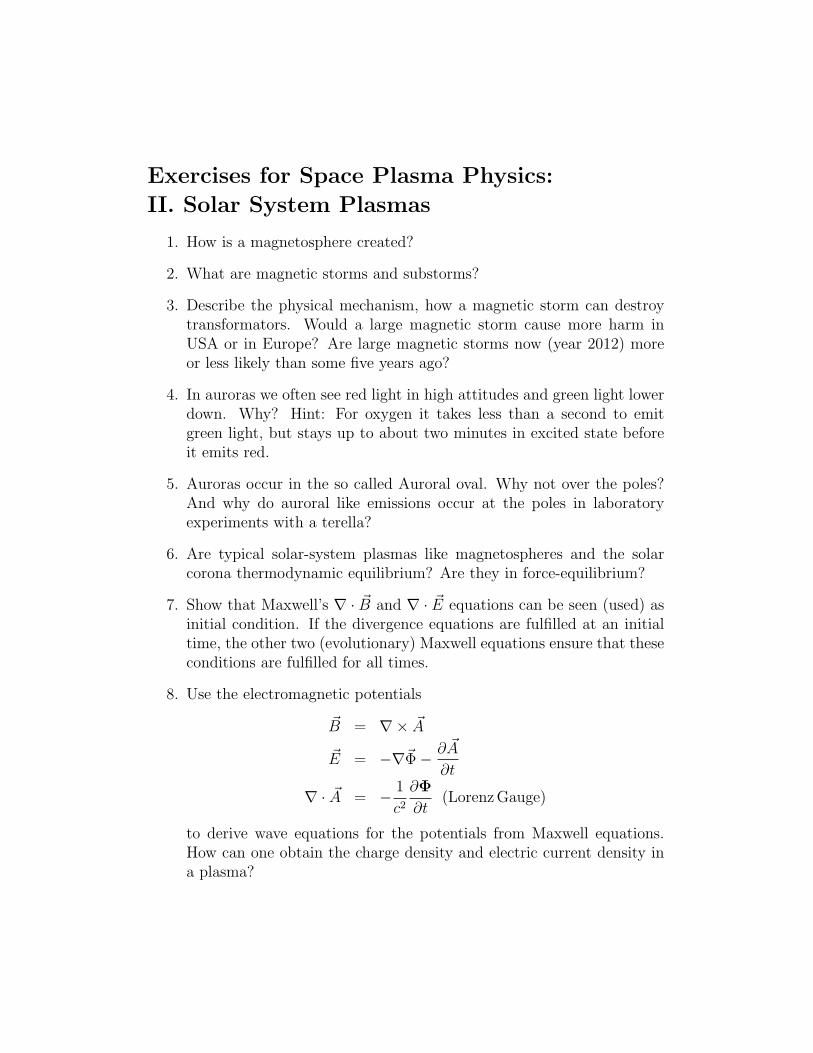
Exercises for Space Plasma Physics:
II. Solar System Plasmas
1. How is a magnetosphere created?
2. What are magnetic storms and substorms?
3. Describe the physical mechanism, how a magnetic storm can destroytransformators. Would a large magnetic storm cause more harm inUSA or in Europe? Are large magnetic storms now (year 2012) moreor less likely than some five years ago?
4. In auroras we often see red light in high attitudes and green light lowerdown. Why? Hint: For oxygen it takes less than a second to emitgreen light, but stays up to about two minutes in excited state beforeit emits red.
5. Auroras occur in the so called Auroral oval. Why not over the poles?And why do auroral like emissions occur at the poles in laboratoryexperiments with a terella?
6. Are typical solar-system plasmas like magnetospheres and the solarcorona thermodynamic equilibrium? Are they in force-equilibrium?
7. Show that Maxwell’s ∇ · ~B and ∇ · ~E equations can be seen (used) asinitial condition. If the divergence equations are fulfilled at an initialtime, the other two (evolutionary) Maxwell equations ensure that theseconditions are fulfilled for all times.
8. Use the electromagnetic potentials
~B = ∇× ~A
~E = −∇~Φ−∂ ~A
∂t
∇ · ~A = −1
c2
∂Φ
∂t(LorenzGauge)
to derive wave equations for the potentials from Maxwell equations.How can one obtain the charge density and electric current density ina plasma?

5/3/2012
1
Space Plasma Physics Thomas Wiegelmann, 2012
1. Basic Plasma Physics concepts
2. Overview about solar system plasmas
3. Single particle motion, Test particle model
4. Statistic description of plasma, BBGKY- Hierarchy and kinetic equations
5. Fluid models, Magneto-Hydro-Dynamics
6. Magneto-Hydro-Statics
7. Stationary MHD and Sequences of Equilibria
Plasma Models
Plasma models - Test particles:
Study motion of individual charged particles under
the influence of external electro-magnetic (EM) fields
- Kinetic models:
Statistic description of location and velocity of
particles and their interaction + EM-fields.
(Vlasov-equation, Fokker-Planck eq.)
- Fluid models:
Study macroscopic quantities like density, pressure,
flow-velocity etc. + EM-fields (MHD + multifluid models)
- Hybrid Models: Combine kinetic + fluid models
Single particle motion, Test particle model
• What is a test particle?
• Charged particles homogenous magnetic
fields => Gyration
• Charged particles in inhomogenous fields
=> Drifts
• Adiabatic invariants
• Magnetic mirror and radiation belts
Test particles:
Equation of Motion, Lorentz-force:
In the test-particle approach the charged
particles move under the influence of
electric and magnetic fields.
Back-reaction of the particles
is ignored => model is not self-consistent.
Test particles, special cases (calculate on blackboard + exercises)
• Static homogenous electric field, no B-field
• Static homgeneous magnetic field
=> Gyration, magnetic moment
• Static, hom. electromagnetic fields (exercise)
• Static inhomogeneous B-field.
• Homogeneous, time-varying electromo-
magnetic fields (exercise).
• Generic cases of time-varying inhomogenous
EM-fields => Treat numerically.
Particles in magnetic field
Kinetic energy is a constant of motion in B-Fields
In B-Fields particles (Electrons, Protons) gyrate
Larmor (or gyro)
frequency
Larmor radius
5/3/2012
2
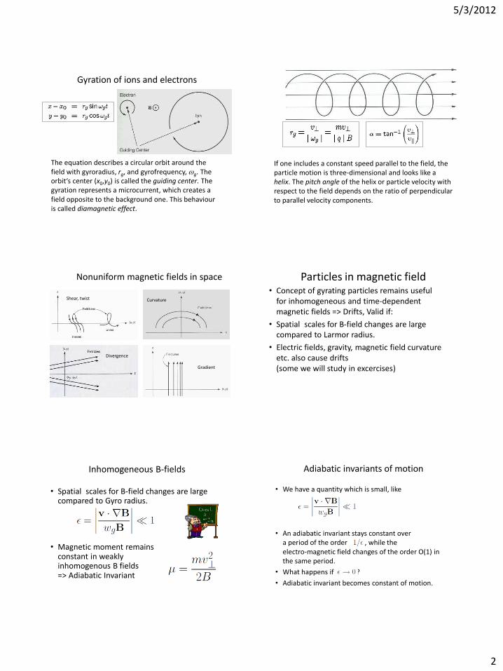
Gyration of ions and electrons
The equation describes a circular orbit around the
field with gyroradius, rg, and gyrofrequency, g. The
ラヴHキデけゲ center (x0,y0) is called the guiding center. The
gyration represents a microcurrent, which creates a
field opposite to the background one. This behaviour
is called diamagnetic effect.
If one includes a constant speed parallel to the field, the
particle motion is three-dimensional and looks like a
helix. The pitch angle of the helix or particle velocity with
respect to the field depends on the ratio of perpendicular
to parallel velocity components.
Nonuniform magnetic fields in space
Curvature
Gradient
Shear, twist
Divergence
Particles in magnetic field • Concept of gyrating particles remains useful
for inhomogeneous and time-dependent
magnetic fields => Drifts, Valid if:
• Spatial scales for B-field changes are large
compared to Larmor radius.
• Electric fields, gravity, magnetic field curvature
etc. also cause drifts
(some we will study in excercises)
Inhomogeneous B-fields
• Spatial scales for B-field changes are large compared to Gyro radius.
• Magnetic moment remains constant in weakly inhomogenous B fields => Adiabatic Invariant
Adiabatic invariants of motion
• We have a quantity which is small, like
• An adiabatic invariant stays constant over
a period of the order , while the
electro-magnetic field changes of the order O(1) in
the same period.
• What happens if ?
• Adiabatic invariant becomes constant of motion.
5/3/2012
3
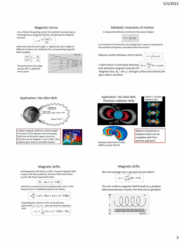
Magnetic mirror
Let us follow the guiding center of a particle moving along an
inhomogeneous magnetic field by considering the magnetic
moment:
where we used the pitch angle . Apparently, pitch angles at
different locations are related by the corresponding magnetic
field strengths:
The point where the angle
reaches 90o is called the
mirror point.
Adiabatic invariants of motion
In classical Hamiltonian mechanics the action integral
is an invariant of motion for any change that is slow as compared to
the oscillation frequency associated with that motion.
Magnetic flux, = B rg2, through surface encircled by the
gyro orbit is constant.
ひBounce motion between mirror points
ひ Drift motion in azimuthal direction,
with planetary magnetic moment M
Application: Van Allen Belt
A dipole magnetic field has a field strength
minumum at the equator and converging
field lines at the polar regions (mirrors).
Particles can be trapped in such a field. They
perform gyro, bounce and drift motions.
Application: Van Allen Belt,
Planetary radiation belts
J┌ヮキデWヴけゲ variable
radiation belt
Motion of particles in
radiation belts can be
modelled with Test-
particle approach. Radiation Belt Storm Probes
(RBSP), launch 2012(?)
Magnetic drifts Inhomogeneity will lead to a drift. A typical magnetic field
in space will have gradients, and thus field lines will be
curved. We Taylor expand the field:
where B0 is measured at the guiding center and r is the
distance from it. Modified equation of motion:
Expanding the velocity in the small drift plus
gyromotion, v = vg + v , then we find the stationary
drift:
Magnetic drifts
We time average over a gyroperiod and obtain:
The non-uniform magnetic field B leads to a gradient
drift perpendicular to both, the field and its gradient:

5/3/2012
4
General force drifts
By replacing the electric field E in the drift formula by any
field exerting a force F/q, we obtain the general guiding-
center drift:
In particular when the field lines are curved, the centrifugal
force is
where Rc is the local radius of
curvature.
Summary of guiding center drifts
Associated drifts are corresponding drift currents.
Try to calculate these
Drifts as excercise
Gyrokinetic approach
• We can distinguish the motion of charged
particles into gyration of the particle and motion of
the gyration center.
• An exact mathematical treatment is possible
within Hamilton mechanics by using non-canonical
transformation.
• => Guiding-center approximation.
[Outside scope of this Lecture, see Balescue,
Transport-Processes in Plasma, Vol. 1, 1988]
• Guiding center approach remains useful concept
for selfconsistent kinetic plasma models.
Magnetic dipole field At distances not too far from
the surface the E;ヴデエけゲ
magnetic field can be
approximated by a dipole
field with a moment:
ME = 8.05 1022 Am2
Measuring the distance in
units of the E;ヴデエけゲ radius, RE,
and using the equatorial
surface field, BE (= 0.31 G),
yields with the so-called L-
shell parameter (L=req/RE) the
field strength as a function of
latitude, , and of L as:
Dipole latitudes of mirror points
Equatorial pitch angle in degrees
Latitude of mirror
point depends only
on pitch angle but
not on L shell
value.
Bounce period as function of L shell
Bounce period, b, is the time
it takes a particle to move
back and forth between the
two mirror points (s is the
path length along a given
field line).
Energy, W, is
here 1 keV and
eq = 30o.

5/3/2012
5
Equatorial loss cone for different L-values
If the mirror point lies
too deep in the
atmosphere (below
100 km), particles will
be absorbed by
collisions with
neutrals.
The loss-cone width depends only on L but
not on the particle mass, charge or energy.
Period of azimuthal magnetic drift motion
Here the energy,
W, is 1 keV and
the pitch angle:
eq = 30o and 90o.
Drift period is of order of several days. Since the magnetospheric
field changes on smaller time scales, it is unlikely that particles
complete an undisturbed drift orbit. Radiation belt particles will
thus undergo radial (L-shell) diffusion!
Summary: Single particle motion
ひ Gyromotion of ions and electrons arround
magnetic field lines.
ひ Inhomogeneous magnetic fields, electric fields
and other forces lead to particle drifts
and drift currents.
ひ Bouncing motion of trapped particles to model
radiation belt.
ひ Constants of motion and adiabatic invariants.
ひ So far we studied particles in external EM-fields and
ignored fields and currents created by the charged
particles and collision between particles.

Exercises for Space Plasma Physics:
III. Single particle motion
1. Under which conditions is the test-particle approach a suitable approx-imation?
2. What are constants of motions? What are adiabatic invariants?
3. What conditions have to be fulfilled that the motion of charged particlescan be described as Drift?
4. How do gyro-radius and frequency change with the magnetic fieldstrength, particle mass, charge and temperature?
5. How do electrons (charge −e, mass me) and ions (charge +e, mass mi
) move under the influence of a constant homogeneous magnetic field~B = B0~ez and
(a) A constant homogeneous electric field ~E = E0 ~ex
(b) A homogenous, but slowly temporal varying electric field
~E = E(t) ~ex
Hint: In the moving frame (Lorentz transform of E) a free particle
does not feel an electric field ~E′
= ~E + ~v ×~B = 0 and you can
average over the gyroperiod assuming that the temporal changesof the electric field are much slower than the gyro-frequency.
(c) Do these drift motions produce electric currents? If yes, calculatethem.

5/10/2012
1
Space Plasma Physics Thomas Wiegelmann, 2012
1. Basic Plasma Physics concepts
2. Overview about solar system plasmas
3. Single particle motion, Test particle model
4. Statistic description of plasma, BBGKY- Hierarchy and kinetic equations
5. Fluid models, Magneto-Hydro-Dynamics
6. Magneto-Hydro-Statics
7. Stationary MHD and Sequences of Equilibria
Plasma Models
Statistical description of a plasma
• The complete statistic description of a
system with N particles is given by the
distribution function
• Hyperspace for N particles has dimension 6 N +1
• N is typically very large (For Sun: N~ 1057 )
=> No chance to compute or estimate F
Liouville Equation
The many body distribution
obeys the Liouville equation
after Joseph Liouville 1809-1889
acceleration of particle i due to external and interparticle forces
Phase space
Six-dimensional
phase space with
coordinates axes x
and v and volume
element dxdv
Many particles (i=1, N) having
time-dependent position xi(t)
and velocity vi(t). The particle
path at subsequent times (t1,..,
t5) is a curve in phase space
Maxwellian velocity distribution function
The general equilibrium VDF in a uniform thermal plasma is the
Maxwellian (Gaussian) distribution.
The average velocity spread (variance) is, <v> =
(2kBT/m)1/2, and the mean drift velocity, v0.
5/10/2012
2
Anisotropic model velocity distributions
The most common anisotropic VDF in a uniform thermal plasma is the bi-
Maxwellian distribution. Left figure shows a sketch of it, with T > T .
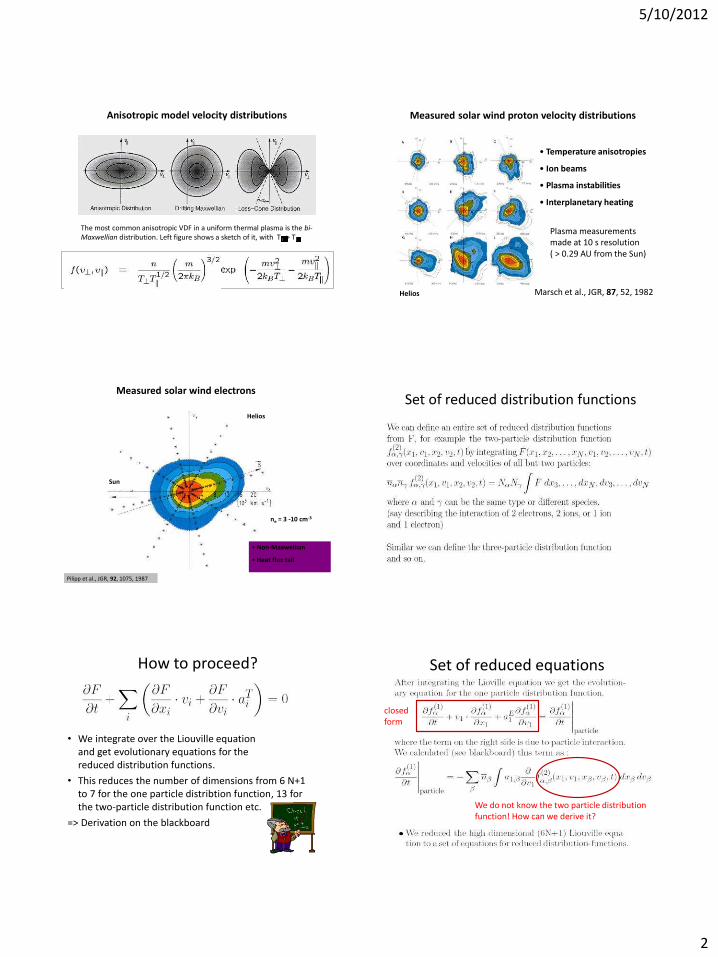
Measured solar wind proton velocity distributions
ひ Temperature anisotropies
ひ Ion beams
ひ Plasma instabilities
ひ Interplanetary heating
Plasma measurements
made at 10 s resolution
( > 0.29 AU from the Sun)
Marsch et al., JGR, 87, 52, 1982 Helios
Measured solar wind electrons
Sun
ひ Non-Maxwellian
ひ Heat flux tail
Pilipp et al., JGR, 92, 1075, 1987
Helios
ne = 3 -10 cm-3
Set of reduced distribution functions
How to proceed?
• We integrate over the Liouville equation
and get evolutionary equations for the
reduced distribution functions.
• This reduces the number of dimensions from 6 N+1
to 7 for the one particle distribtion function, 13 for
the two-particle distribution function etc.
=> Derivation on the blackboard
Set of reduced equations
closed
form
We do not know the two particle distribution
function! How can we derive it?
5/10/2012
3
• Problem: Equation for the one particle distribution
function contains the two particle distribution
function on the right side.
• In principle we know, how to derive that one:
Do the corresponding integration over the
Liouville equation (we do not show that
explicitely in this lecture)
• Problem: Equation for the two particle distribution
function contains the 3-particle
distribution function on right side, and so on.
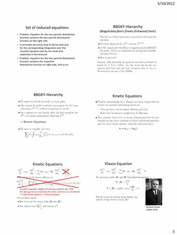
Set of reduced equations BBGKY-Hierarchy (Bogoliubov,Born,Green,Kirkwood,Yvon)
BBGKY-Hierarchy Kinetic Equations
Kinetic Equations
Simplest approach: Neglect the binary-collision rate. Only
the average forces created by the other particles are considered
=> Collisionless plasma => Vlasov equation
Vlasov Equation
Anatoly Vlasov
(1908-1975)

5/10/2012
4
Vlasov equation
The Vlasov equation
expresses phase space
density conservation.
A 6D-volume element
evolves like in an
incompressible fluid.
Vlasov equation is
nonlinear via closure with
M;┝┘Wノノけゲ equations.
Vlasov Equation
Macroscopic variables of a plasma
needed in
Vlavov-Maxwell
system
Macroscopic variables of a plasma
needed in Vlavov-Maxwell system
Macroscopic variables of a plasma Macroscopic variables of a plasma

5/10/2012
5
Vlasov-Maxwell Equations kinetic description of a collisionless plasma
• Vlasov Equation conserves particles
• Distribution functions remains positive
• Vlasov equation has many equilibrium solutions
Properties of Vlasov Equation
Stability of Vlasov equilibria Example: The well known
Maxwell-Boltzmann-distribution
James Clerk Maxwell,
1831-1871
Ludwig Boltzmann,
1844-1906
is stable! (Proof on blackboard)
Further Examples
• Drifting Maxwellian ?
• Maxwellian with a non-thermal feature ?
Investigate stability
as an excercise.
Kinetic equations of first order
• Vlasov approach: neglect 2 particle
distribution function completely
• Now we make a more sophisticated approach,
the Mayer cluster expansion.

5/10/2012
6
Mayer cluster expansion
Particles are independent
from each other
Correlation of
the 2 particles
Collisions
Plasmas may be collisional (e.g., fusion plasma) or
collisionsless (e.g., solar wind). Space plasmas are
usually collisionless. => Vlasov equation
Ionization state of a plasma:
ひ Partially ionized: E;ヴデエけゲ ionosphere or S┌ミけゲ
photosphere and chromosphere, dusty and
cometary plasmas
=> Collisions with neutrals dominate
ひ Fully ionized: S┌ミけゲ corona and solar wind and
most of the planetary magnetospheres
=> Coulomb collisions or collisionless
Coulomb collisions
Charged particles interact via the Coulomb force
over distances much larger than atomic radii, which
enhances the cross section as compared to hard
sphere collisions, but leads to a preference of small-
angle deflections.
Impact or collision parameter, dc, and scattering angle, c.
Models for the collision terms
Neutral-ion collisions are
described by a Maxwell
Boltzmann collision terms as in
Gas-dynamics. (fn : distribution
function of neutrals, n collision
frequency):
Coulomb Collisions lead to the
Fokker-Planck-Equation which
can often be described as a
diffusion process.
Further sophistications are to take into account that Coulomb
collisions occur not in vaccum, but are Debye-shielded and
to consider wave-particle interactions.
Kinetic Equations
• In Kinetic theory we have a statistic description in
a 6D phase space (configuration and velocity space).
• Kinetic equations are a first order approximation of
the BBGKY-Hierarchy.
• Equation for Particle distribution function is coupled
with Maxwell-equations => Difficult to solve.
• Most space plasmas are collisionless => Vlasov equation
• Collission terms depend on nature of process:
- collision with neutrals => Maxwell-Boltzmann
- Coloumb collisions: Fokker-Planck
- Coloumb c. with Debye-shielding => Lennard Balescu
How to proceed?
• Due to the nonlinear coupling with Maxwell-equations,
the Kinetic equations are difficult to solve.
• In numerical simulations one has to resolve relevant
plasma scales like Debye-length, gyro-radii of electrons
and ions and also the corresponding
temporal scales (gyro-frequencies, plasma frequencies),
which are orders of magnitude smaller
and faster as the macroscopic scales (size of
magnetosphere or active region)
• We often not interested in details of the
velocity distribution function.
• => Integration over the velocity space lead to fluid
equations like MHD (3D instead of 6D space)

Exercises for Space Plasma Physics:
IV. Kinetic equations
1. What is the difference between the Vlasov-, Boltzmann- and Fokker-Planck equation?
2. Why do physicists use the Fokker-Planck equation in fully ionized plas-mas instead of the Boltzmann equation used for normal gases?
3. How does the entropy S = −
∑
α
∫
fα ln fα dx dv evolve in a VlasovMaxwell system?
4. In the lecture we showed the Mayer-Cluster-expansion for the two-particle distribution function f
(2)α,β. Can you imagine, how the cor-
responding expansion for a three particle-distribution function f(3)α,β,γ
looks like? Are three-particle correlations assumed to be more or lessimportant than two-particle correlations in space plasmas?
5. Check if the following distribution functions are stable or unstable:
• Drifting Maxwellian (with Drift velocity uD):
f(v) ∝ exp
(
−
m (v − uD)2
2 kb T
)
• Maxwellian with a non-thermal feature like a drifting beam
f(v) = exp
(
−
mv2
2 kb T
)
+ ǫ exp
(
−10 ·m (v − uD)
2
2 kb T
)

5/24/2012
1
Space Plasma Physics Thomas Wiegelmann, 2012
1. Basic Plasma Physics concepts
2. Overview about solar system plasmas
3. Single particle motion, Test particle model
4. Statistic description of plasma, BBGKY- Hierarchy and kinetic equations
5. Fluid models, Magneto-Hydro-Dynamics
6. Magneto-Hydro-Statics
7. Stationary MHD and Sequences of Equilibria
Plasma Models
Multi-fluid theory
ひ Full plasma description in terms of particle
distribution functions (VDFs), fs(v,x,t), for species, s.
ひ For slow large-scale variations, a description in terms
of moments is usually sufficient -> multi-fluid (density,
velocity and temperature) description.
ひ Fluid theory is looking for evolution equations for the
basic macroscopic moments, i.e. number density,
ns(x,t), velocity, vs(x,t), pressure tensor, Ps(x,t), and
kinetic temperature, Ts(x,t). For a two fluid plasma
consisting of electrons and ions, we have s=e,i.
Magneto-hydro-dynamics (MHD)
• Fluid equations reduce from the 6D space
from kinetic theory to our usual 3D configuration
space (and the time).
• In Fluid theory, we miss some important physics,
however. With single fluid MHD even more than
multi fluid (2 Fluid: electrons and ions).
• 3 fluid (+neutral particles) and 4 fluid models
are popular in space plasma physics, too, also
one can use different fluids for different Ion-species.
• Hybrid-model: Ions treated as particles and electrons
as fluid.
Fluid models, Magneto-Hydro-Dynamics
• If we solved the kinetic equations (Vlasov or Fokker-
Planck-equation) we derive macroscopic variables by
taking velocity-moments of the distribution functions.
Fluid models, Magneto-Hydro-Dynamics
• Solving the kinetic equations is, however, very
difficult, even numerically. One has to resolve
all spatial and temporal plasma scales like
Debey-length/frequency, Gyro-radius/frequency etc.
• In space plasmas these scales are often orders
of magnitudes smaller as the macroscopic scales we
are interested in (like size of solar active regions or
planetary magnetospheres).
• Solution: We take velocity-moments over the kinetic
equations (Vlasov-equation), instead of (generally
unknown) solution of the kinetic equation.
Continuity equation
Evolution equations of moments are obtained by taking
the corresponding moments of the Vlasov equation:
Taking the zeroth moment yields
for the first term:
In the second term, the velocity
integration and spatial differentiation
can be interchanged which yields a
divergence:
In the force term, a partial
integration leads to a term, which
does not contribute.

5/24/2012
2
Continuity equation
We have again (like in BBGKY-hierarchy) the
problem, that the equation for the 0-moment
(density) contains the first moment
(velocity v or momentum nv).
Momentum equation
The evolution equation for the flow velocity/momentum is
obtained by taking the first moment of the Vlasov equation:
Since the phase space coordinate v
does not depend on time, the first
term yields the time derivative of the
flux density:
In the second term, velocity integration and spatial
differentiation can be exchanged, and v(v· x) = x ·(vv) be
used. With the definition of the pressure tensor we get:
In the third term, a partial integration with respect to the
velocity gradient operator v gives the remaining integral:
We can now add up all terms and obtain the final result:
This momentum density conservation equation for species s
corresponds to the Navier-Stokes equation for neutral fluids.
In a plasma the equation becomes more complicated due to
coupling with Maxwell-equations via the Lorentz-force.
This equation for the first-moment
(velocity, momentum) contains the second
moment (pressure tensor).
And so on .....
Equation for moment k, contains always the
moment k+1 => Hierarchy of moments
Momentum equation or equation of motion
Hierarchy of moments
• As in kinetics (BBGKY) we have to cut the hierarchy
somewhere by making suitable approximations.
• Number of (scalar) variables increase by taking
higher orders of moments v^n.
• MHD, 5 moments: density, 3 components of velocity
and a scalar (isotropic) pressure (or temperature).
These 5 moments are called plasmadynamic variables.
• Fluid equations with a higher number of moments
(13, 21, 29, 37, ...) are possible and take anisotropy
and approximated correction terms (for cutting the
infinite chain of hierarchy-equations) into account.
Energy equation
The equations of motion do not close, because at any order a new
moment of the next higher order appears (closure problem), leading
to a chain of equations. In the momentum equation the pressure
tensor, Ps, is required, which can be obtained from taking the seond-
order moment of Vノ;ゲラ┗けゲ equation. The results become
complicated. Often only the trace of Ps, the isotropic pressure, ps, is
considered, and the traceless part, P's ,the stress tensor is separated,
which describes for example the shear stresses.
Full energy (temperature, heat transfer) equation:
The sources or sinks on the right hand side are related to heat
conduction, qs, or mechanical stress, P's.

5/24/2012
3
Equation of state A truncation of the equation hierarchy can be achieved
by assuming an equation of state, depending on the form
of the pressure tensor.
If it is isotropic, Ps = ps1, with the unit dyade, 1, and ideal
gas equation, ps= nskBTs, then we have a diagonal matrix:
ひ Isothermal plasma: Ts = const
ひ Adiabatic plasma: Ts = Ts0 (ns/ns0) -1, with the adiabatic
index = cP/cV = 5/3 for a mono-atomic gas.
ひ Incompressible plasma Div v =0
Equation of state
Due to strong magnetization, the plasma pressure is often
anisotropic, yet still gyrotropic, which implies the form:
ひ T B -> perpendicular heating in increasing field
ひ T|| (n/B)2 -> parallel cooling in declining density
with a different pressure (temperature) parallel and perpendicular
to the magnetic field. Then one has two energy equations, which
yield (without sinks and sources) the double-adiabatic equations
of state:
Measured solar wind proton velocity distributions
Non-isotropic particle
distribution functions lead
to pressure tensor (instead
of scalar pressure) in fluid
approach.
Marsch et al., JGR, 87, 52, 1982 Helios
One-fluid theory
Consider simplest possible plasma of fully ionized hydrogen with
electrons with mass me and charge qe = -e, and ions with mass mi
and charge qi = e. We define charge and current density by:
Usually quasineutrality applies, ne= ni, and space charges
vanish, = 0, but the plasma carries a finite current, i.e. we
still need an equation for j. We introduce the mean mass,
density and velocity in the single-fluid description as
One-fluid momentum equation Constructing the equation of motion is more difficult because
of the nonlinear advection terms, nsvsvs.
The equation of motion is obtained by adding these two equations
and exploiting the definitions of , m, n, v and j. When multiplying
the first by me and the second by mi and adding up we obtain:
Here we introduced the total pressure tensor, P = Pe + Pi . In the
nonlinear parts of the advection term we can neglect the light
electrons entirely.
Magnetohydrodynamics (MHD) With these approximations, which are good for many quasineutral
space plasmas, we have the MHD momentum equation, in which
the space charge (electric field) term is also mostly disregarded.
Note that to close the full set, an equation for the current
density is needed. For negligable displacement currents, we
simply use AマヮWヴWけゲ law in magnetohydrodynamics and B as a
dynamic variable, and replace then the Lorentz force density
by:

5/24/2012
4
Generalized Oエマけゲ law
The evolution equation for the current density, j, is derived
by use of the electron equation of motion and called
generalized Oエマけゲ law. It results from a subtraction of the
ion and electron equation of motion. The nonlinear
advection terms cancel in lowest order. The result is:
The right hand sides still contain the individual densities,
masses and speeds, which can be eliminated by using that
me/mi << 1, ne ni
Generalized Oエマけゲ law
We obtain a simplified equation:
Key features in single-fluid theory: Thermal effects on j enter
only via, Pe, i.e. the electron pressure gradient modulates the
current. The Lorentz force term contains the electric field as
seen in the electron frame of reference.
Generalized Oエマけゲ law
Omitting terms of the order of the small mass ratio, the
fluid bulk velocity is, vi = v. Using this and the
quasineutrality condition yields the electron velocity as: ve
= v - j/ne. Finally, the collision term with frequency c can
be assumed to be proportional to the velocity difference,
and use of the resistivity, =me c/ne2, permits us to write:
Generalized Oエマけゲ law
The resulting Oエマけゲ law can then be written as:
The right-hand side contains, in a plasma in addition to the
resistive term, three new terms: Hall term, electron pressure,
contribution of electron inertia to current flow.
Popular further simplifications are:
• Resistive MHD:
• Ideal MHD:
Magnetic tension
The Lorentz force or Hall term introduces a new effect in a
plasma which is specific for magnetohydrodynamics:
magnetic tension, giving the conducting fluid stiffness. For
slow variations AマヮWヴWけゲ law can be used to derive:
Applying some vector algebra to the right hand side gives:
magnetic
pressure
Plasma beta
Starting from the MHD equation of motion for a plasma at
rest in a steady quasineutral state, we obtain the simple force
balance:
which expresses magnetohydrostatic equilibrium, in which
thermal pressure balances magnetic tension. If the particle
pressure is nearly isotropic and the field uniform, this leads to
the total pressure being constant:
The ratio of these two terms
is called the plasma beta:

5/24/2012
5
Requirements for the validity of MHD
Variations must be large and slow, < gi and k < 1/rgi,
which means fluid scales must be much larger than
gyro-kinetic scales. Consider Oエマけゲ law:
Convection, Hall effect, thermoelectricity, polarization, resistivity
/ c gi / c
Only in a strongly collisional
plasma can the Hall term be
dropped. In collisionless MHD the electrons
are frozen to the field.
MHD-equations (fluid part, including gravity)
source:
Neukirch 1998
MHD-equations (Maxwell-part + Oエマけゲ law) Summary: Fluid equations, MHD
ひ Multi-fluid theory
ひ Equation of state
ひ Single-fluid theory
ひ Generalised Oエマけゲ law
ひ Magnetic tension and plasma beta
ひ Validity of magnetohydrodynamics
How to proceed?
• We will look at example solution of the MHD, which
are relevant for space plasmas.
• First we compute static equilibria (no plasma-flow,
no time dependence) => Magneto-statics
• Stationary solutions (no time dependence, but
including stationary plasma flows)
• Sequences of equilibria (slow time dependence)
• Time dependent solutions, waves, instabilities
and magnetic reconnection.
Exercises for Space Plasma Physics:
V. MHD
1. Remember the main steps we needed to derive the MHD-equations
from a statistic particle model.
2. Under which conditions is the MHD-model valid?
3. Explain the different terms in the MHD-equations qualitatively.
4. Explain ideal and resistive MHD.
5. Are space plasmas typically ideal or resistive plasmas?
6. How can Ohm’s law as used in MHD be derived from a two-fluid model?
7. In MHD one often compares different energy forms like the magnetic
pressure pB = B2
2µ0
and the kinematic energy density Ekin = ρv2
2with the
plasma pressure p. How do pB and Ekin evolve in time? Hint: derive
the corresponding evolutionary equations from the MHD momentum-
transport equation.

5/31/2012
1
Space Plasma Physics Thomas Wiegelmann, 2012
1. Basic Plasma Physics concepts
2. Overview about solar system plasmas
3. Single particle motion, Test particle model
4. Statistic description of plasma, BBGKY- Hierarchy and kinetic equations
5. Fluid models, Magneto-Hydro-Dynamics
6. Magneto-Hydro-Statics
7. Stationary MHD and Sequences of Equilibria
Plasma Models
Magneto-Hydro-Statics (MHS) • No time dependence and no plasma flows
• More precise: The dynamic terms in MHD
are small compared with static forces
(Lorentz-force, plasma pressure gradient, gravity)
• Sequences of equilibria (slow temporal changes) and
equilibria with stationary plasma
flow are studied in the next lecture.
Parts of this lecture are based on the course INTRODUCTION TO
THE THEORY OF MHD EQUILIBRIA
given by Thomas Neukirch in St. Andrews 1998.
Magneto-hydro-statics (MHS) source:
Neukirch 1998 MHS-equations (Maxwell-part + Oエマけゲ law)
MHS
With the vector potential one equation
(solenoidal condition) is already solved automatically.
Why is it useful to study MHS ?
• From a fundamental point of view we can regard the
MHD equations as a set of equations describing
extremely complicated dynamical systems. In the
study of dynamical systems it is always useful to start
with a study of the simplest solutions. These are
usually the stationary states and their bifurcation
properties, in the MHD case the static equilibria.
• From the point of view of modelling, many physical
processes in plasma systems occur slowly, i.e. on
time-scales which are much longer than the typical
time-scale of the system.

5/31/2012
2
Dimensionless Force-balance
• The magnetostatic equations in dimensionless form
can be used to evaluate the relative importance of
the different terms.
• For a small the gravity force can be neglected.
This is usually fulfilled in magnetospheric plasmas.
• If is small, too we can neglect also the plasma-
pressure gradient in the force-balance
=> Force-free fields, a valid assumption in most parts
of the solar corona.
• To lowest order we have the MHS force balance
equation as fundamental equation and the time appears
merely as a parameter.
• The fundamental importance of this quasi-static
approximation lies in the fact that sequences of MHS
equilibria can be used to model the slow evolution of
plasma systems. (Growth phase of magnetospheric
substorms, evolution of non-flaring solar active regions)
• Sequences have to satisfy the constraints imposed by
the other equations, especially Ohm's law and the
continuity equations.
• These constraints usually lead to very complicated
integro-differential problems which are difficult to solve.
Systems with symmetries
• In the generic 3D case the MHS-equations are
still difficult to solve due to their non-linearities.
• We consider now system with symmetries, e.g.
in cartesian geometry (x,y,z) equilibria which are
invariant in y. => 2D
• One can use also spherical, cylinder or helical symmetry,
but the mathematics become a bit more complicated.
• We represent the magnetic field as:
Vitalii Dmitrievich
Shafranov, born 1929 Source: Physics Uspekhi
53 (1) 101 (2010)
Harold Grad
1923-1986 Source: AIP.org
Grad-Shafranov-Equation
In 2D the
MHS-equations
(without gravity)
reduce to a single
partial differential
equation.
• We reduced the MHS to a single partial
differential equations.
• The equation still contains the unknown pressure
profile A -> p(A) and magnetic shear B_y
• Obviously p(A) has to be positive.
• For p(A)=A^2 the GSE becomes linear (popular choice)
• Within MHD p(A) is arbitrary, but
it is possible to derive the pressure
profile from kinetic theory.
Grad-Shafranov-Equation

5/31/2012
3
Linear Grad-Shafranov-Equation
Non-linear Grad-Shafranov-Equation Kinetic theory for p(A)
• With invariance in y we have 2 constants of motion for the
particles: Hamiltionian and momentum in y
• For a local thermic equilibrium the particle distribution
function for each species is given by a drifting Maxwelian:
• Macroscopic (fluid) quantities like the particle density, current density and pressure for electrons and ions, we get by integration over the velocity space. The plasma pressure is isotropic per construction by a Maxwellian.
• We get the total pressure by adding the partial pressure of electron and ions.
• Assuming quasi-neutrality (n_i=n_e) allows to eliminate the electro static potential and we get:
• We derived the GSE earlier from MHD, but it is valid also in kinetic theory and can be used to compute Vlasov-equilibria (e.g., intial states for kinetic simulations)
How to get B_y(A) ?
• The magnetic shear of a configuration like a
coronal magnetic loop can in principle be computed
from the displacement of footpoints.

5/31/2012
4
Non-linear GSE, Liouville solution
• We choose :
• And derive the solution:
Non-linear GSE, 1D Harris (1962) Sheet
Used to describe
current sheets in
space plasmas.
Valid also in
kinetic approach.
Source of pictures: Nickeler et al. 2010
Non-linear GSE, Magnetosphere solution (Schindler & Birn 2004) Including gravity
• External gravity force:
• Force-balance:
• Plasma pressure is not constant along field lines
• Pressure gradient needs to be compensated by
gravity force, as the Lorentz-force vanishes parallel
to the magnetic field
• We use again:
• Similar as for the Grad-Shafranov (GS) equation we get
• And the force balance:
Including gravity Including gravity
This equation is fulfilled for:

5/31/2012
5
Including gravity
• Inserting this into the last equation:
• And the force balance equation becomes:
• The coefficients must vanish because
are linear independent.
• Finally we have to solve:
• To proceed we make now assumptions about the
equation of state, e.g. isothermal plasma (simplest
approach and the only one we consider here explicitely )
• A polytropic equation of state is also possible.
• Most realistic (and most complicated) would be to
solve the energy equation.
Including gravity
Including gravity, isothermal plasma 3D configurations
• Analytic we can find 3D-equilibria without
symmetry only in special cases.
• We can use Euler potentials:
• And transform the force balance to:
3D configurations
Instead of a single partial differential equation
(Grad-Shafranov) we get a system of coupled nonlinear
equations => Extremely difficult to solve
Special cases in 3D: Force-free magnetic fields
A special equilibrium of ideal MHD (often used in case of the
solar corona) occurs if the beta is low, such that the pressure
gradient can be neglected. The stationary plasma becomes force
free, if the Lorentz force vanishes:
This condition is guaranteed if the current flows along the field:
By taking the
divergence, one finds
that L(x) is constant
along any field line:
5/31/2012
6
Magneto-Hydro-Statics (MHS)
• Equilibrium structures (no time dependence,
no plasma flow) are important and often
approximately a reasonable assumption for
space plasmas during quiet times.
• For symmetric configurations, MHS reduces to the
Grad-Shafranov equation (GSE), a single (nonlinear)
partial differential equation.
• GSE remains valid in kinetic theory.
• 3D MHS-equilibria have usually be computed
numerically.
How to proceed?
• Study stationary states with plasma flow.
• The slow evolution of sequences of equilibria
is often constraint, e.g., by the assumption of
ideal MHD, which does not allow topology changes.
• Plasma waves are ubiquitos in space plasma.
• Discontinuities and current sheets.
• Plasma instabilities cause rapid changes and
the equilibrium is lost (ideal and resistive
instabilities).
Exercises for Space Plasma Physics:
VI. Magneto-statics
1. Under which conditions can a plasma described with magneto-hydro-statics (MHS)?
2. Which terms in MHD are neglected to derive the MHS-equations?
3. Give examples for solar system plasmas suitable for MHS models.
4. What is a force-free model? When can it be applied?
5. Can you give an example for a force-free plasmas?
6. Remember the main steps from a 2D-MHS-models to the Grad-Shafranovequation.
7. Now we extend the Grad-Shafranov theory to 2.5D, which means thatall quantities are still invariant in the y-direction, but the magneticfield vector has three components. Use the ansatz
~B = ∇A× ey +Byey
and derive the corresponding Grad-Shafranov equation.
8. How does the Grad-Shafranov-equation (2.5D) look for a force-freeplasma?
6/14/2012
1
Space Plasma Physics Thomas Wiegelmann, 2012
1. Basic Plasma Physics concepts
2. Overview about solar system plasmas
3. Single particle motion, Test particle model
4. Statistic description of plasma, BBGKY- Hierarchy and kinetic equations
5. Fluid models, Magneto-Hydro-Dynamics
6. Magneto-Hydro-Statics
7. Stationary MHD and Sequences of Equilibria
Plasma Models
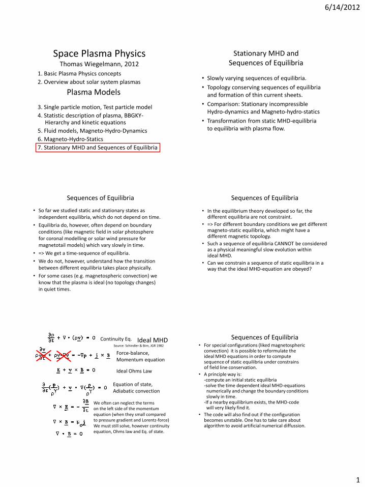
Stationary MHD and
Sequences of Equilibria
• Slowly varying sequences of equilibria.
• Topology conserving sequences of equilibria
and formation of thin current sheets.
• Comparison: Stationary incompressible
Hydro-dynamics and Magneto-hydro-statics
• Transformation from static MHD-equilibria
to equilibria with plasma flow.
Sequences of Equilibria
• So far we studied static and stationary states as
independent equilibria, which do not depend on time.
• Equilibria do, however, often depend on boundary
conditions (like magnetic field in solar photosphere
for coronal modelling or solar wind pressure for
magnetotail models) which vary slowly in time.
• => We get a time-sequence of equilibria.
• We do not, however, understand how the transition
between different equilibria takes place physically.
• For some cases (e.g. magnetospheric convection) we
know that the plasma is ideal (no topology changes)
in quiet times.
• In the equilibrium theory developed so far, the different equilibria are not constraint.
• => For different boundary conditions we get different magneto-static equilibria, which might have a different magnetic topology.
• Such a sequence of equilibria CANNOT be considered as a physical meaningful slow evolution within ideal MHD.
• Can we constrain a sequence of static equilibria in a way that the ideal MHD-equation are obeyed?
Sequences of Equilibria
Ideal MHD
Ideal Ohms Law
Equation of state,
Adiabatic convection
Continuity Eq.
Force-balance,
Momentum equation
Source: Schindler & Birn, JGR 1982
We often can neglect the terms
on the left side of the momentum
equation (when they small compared
to pressure gradient and Lorentz-force)
We must still solve, however continuity
equation, Ohms law and Eq. of state.
• For special configurations (liked magnetospheric convection) it is possible to reformulate the ideal MHD equations in order to compute sequence of static equilibria under constrains of field line conservation.
• A principle way is: -compute an initial static equilibria -solve the time dependent ideal MHD-equations numerically and change the boundary conditions slowly in time. -If a nearby equilibrium exists, the MHD-code will very likely find it.
• The code will also find out if the configuration becomes unstable. One has to take care about algorithm to avoid artificial numerical diffussion.
Sequences of Equilibria

6/14/2012
2
Stationary incompressible MHD
Subsets are
1.) No plasma flow:
Magneto-Hydro-Statics
(MHS)
2.) No magnetic field:
Stationary Incom-
pressibel Hydro-
Dynamics (SIHD)
SIHD
SIHD
Magneto-hydro-statics
vorticity
current density
SIHD and MHS have same mathematical
structure (Gebhardt&Kiessling 92):
MHS SIHD
Stationary incompressible MHD
If plasma flow parallel
to magnetic field
Stationary incompressible MHD • Mathematical structure of hydro-dynamics and
magneto-static is similar.
• We assume, that we found solution of a magneto-
static equilibrium (Grad-Shafranov Eq. in 2D = >
Flux-function or Euler-potentials in 3D).
• We use the similar mathematical structure to
find transformation equations (different flux-
function) to solve stationary MHD.
• We introduce the Alfven velocity
and the Alfven Machnumber
• We limit to sub-Alfvenic flows
here. Pure super-Alfvenic flows can be studied
similar. Somewhat tricky are trans-Alfvenic flows.

6/14/2012
3
• With this approach we can eliminate the plasma
velocity in the SMHD equations and get:
• Obviously the equations reduce to magnetostatics
for M_A=0. The second equation changes キデけゲ sign
from sub- to super-Alfvenic flows.
Stationary incompressible MHD
=> Alfven Machnumber is constant on field lines
• Similar as in the magneto-static case we represent
the magnetic field with a flux-function:
• Flux functions are not unique and we can transform
to another flux function
• The Alfven mach number is constant on field lines:
• We can now eliminate terms containing the
Alfven Mach number by choosing:
Stationary incompressible MHD in 2D
• The stationary incompressible MHD-equations
reduce to a Grad-Shafranov equation
• Any solution we found for the static case can be
used to find a solution for equilibria with flow by:
• Transformation can become complicated, however.
Grad-Shafranov-Equation with flow
Jovian Magnetosphere
• Jupiter: fast rotation 10 h, mass-loading 1000 kg/s
• Dynamics driven largely by internal sources.
• Planetary rotation coupled with internal plasma
loading from the moon Io may lead to additional
currents, departure from equilibrium, magnetospheric
instabilities and substorm-like processes.
• Stationary states of a fast rotating magnetosphere
cannot be modeled with a magneto-static model.
• We have to incorporate the rotation
=> Equilibria with centrifugal force.
Planetary magnetospheres
We use a cylinder geometry and derive the
corresponding Grad-Shafranov Equation.
Source: Neukirch 1998
6/14/2012
4
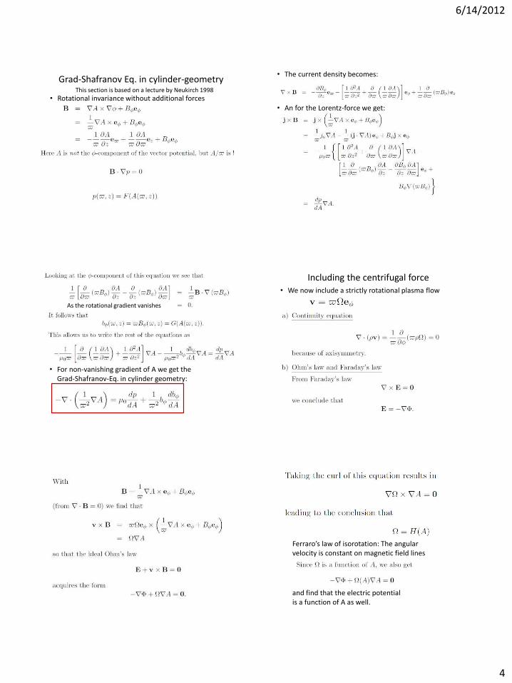
Grad-Shafranov Eq. in cylinder-geometry
• Rotational invariance without additional forces This section is based on a lecture by Neukirch 1998
• The current density becomes:
• An for the Lorentz-force we get:
• For non-vanishing gradient of A we get the
Grad-Shafranov-Eq. in cylinder geometry:
As the rotational gradient vanishes
Including the centrifugal force
• We now include a strictly rotational plasma flow
FWヴヴ;ヴラげゲ ノ;┘ ラa isorotation: The angular
velocity is constant on magnetic field lines
and find that the electric potential
is a function of A as well.

6/14/2012
5
We write the velocity more convenient Momentum Balance Equation
Grad-Shafranov-eq. for rotating systems
• Ferraro's law of isorotation restricts the angular velocity.
Grad-Shafranov-eq. for rotating systems
Sequences of equilibria
• One should not naively consider every sequences of
static equilibria as a physical reasonable temporal
evolution.
• Magnetostatic means, that velocity and time-
dependence are small (and can be neglected)
in the momentum transport.
• We still have to solve continuity equation, ideal
Oエマげゲ law and an equation of state to obtain
a physical meaningful time-sequence of equilibria.
• This can become involved.
• Magnetostatics and stationary Hydrodynamics
are mathematical similar, also the terms have
different physical meaning.
• We can use this property to transform solutions
of MHS to stationary MHD for incompressible
field line parallel plasma flows.
• Rotating systems are restricted by Ferraros law
of isoration and we have to solve two coupled
differential equations.
Stationary MHD

6/14/2012
6
How to proceed?
• Study time dependent system:
• Plasma Waves
• Instabilities
• Discontinuities
• Waves and instabilities occur in MHD as
well as in a kinetic model.
• In discontinuities the Fluid approach often
breaks down and one has to apply kinetic models.

Exercises for Space Plasma Physics:
VII. Stationary MHD
1. Discuss mathematical similarities and differences of MHS and station-ary, incompressible hydro-dynamics.
2. Is this similarity useful to study stationary MHD? Under which condi-tions?
3. What are quasi-static equilibria? Is this a useful concept at all?
4. Euler potentials are defined as ~B = ∇α ×∇β. Discuss briefly advan-tages and disadvantages of using Euler potentials.
5. For simplicity, one often investigates configuration in 2D, which areinvariant in one spatial coordinate (say in y) and uses a flux function
A(x, z) with ~B = ∇A × ~ey. Can you provide the vector potential andthe Euler potentials for a given flux-function?
6. Now let’s consider the full 3D case. Assume you have α and β given.Can you derive a coresponding vector potential ~A?

6/21/2012
1
Physical Processes
8. Plasma Waves, instabilities and shocks
9. Magnetic Reconnection
Applications
10. Planetary Magnetospheres
11. Solar activity
12. Transport Processes in Plasmas
Space Plasma Physics Thomas Wiegelmann, 2012
Electromagnetic wave in a plasma
Electromagnetic waves with a frequency below the
plasma frequency cannot travel into the plasma.
(they become reflected) => Cutoff-frequeny
Exercise: How can this property be used to
measure the (electron) density of a plasma
with EM-waves?
Ideal MHD equations
Plasma equilibria can easily be perturbed and small-amplitude
waves and fluctuations can be excited.
Energy equation omitted, because not needed here.
MHD equilibrium and fluctuations We assume stationary ideal homogeneous conditions as the
intial state of the single-fluid plasma, with vanishing average
electric and velocity fields, overal pressure equilibrium and no
magnetic stresses. These assumptions yield:
These fields are decomposed as
sums of their background initial
values and space- and time-
dependent fluctuations as follows:
Linear perturbation theory
Because the MHD equations are nonlinear (advection term and
pressure/stress tensor), the fluctuations must be small.
-> Arrive at a uniform set of linear equations, giving the
dispersion relation for the eigenmodes of the plasma.
-> Then all variables can be expressed by one, say the
magnetic field.
Usually, in space plasma the background magnetic field is
sufficiently strong (e.g., a planetary dipole field), so that
one can assume the fluctuation obeys:
In the uniform plasma with straight field lines, the field
provides the only symmetry axis which may be chosen
as z-axis of the coordinate system such that: B0=B0ê .
Linearized MHD equations Linarization of the MHD equations leads to three
equations for the three fluctuations, n, v, and B:
Using the adiabatic pressure
law, and the derived sound
speed, cs2 = p0/(min0), leads to
an equation for p and gives:

6/21/2012
2
Linearized MHD equations II
Inserting the continuity and pressure equations, and using the Alfvén
velocity, vA=B0/( 0nmi)1/2, two coupled vector equations result:
Time differentiation of the first and insertion of the second equation yields a
second-order wave equation which can be solved by Fourier
transformation.
Dispersion relation
The ansatz of travelling plane waves,
with arbitrary constant amplitude, v0, leads to the
system,
To obtain a nontrivial solution the determinant must vanish, which
means
Here the magnetosonic speed is given by cms2 = cs
2 + vA2. The wave vector
component perpendicular to the field is oriented along the x-axis, k= k êz+
k êx.
Alfvén waves
Inspection of the determinant shows that the fluctuation in the
y-direction decouples from the other two components and has
the linear dispersion
This transverse wave travels parallel to the field. It is called
shear Alfvén wave. It has no density fluctuation and a
constant group velocity, vgr,A = vA, which is always oriented
along the background field, along which the wave energy is
transported.
The transverse velocity and magnetic field components are
(anti)-correlated according to: vy/vA = ± By/B0, for parallel
(anti-parallel) wave propagation. The wave electric field
points in the x-direction: Ex = By/vA
Magnetosonic waves
The remaing four matrix elements couple the fluctuation
components, v and v . The corresponding determinant reads:
This bi-quadratic equation has the roots:
which are the phase velocities of the compressive fast and
slow magnetosonic waves. They depend on the propagation
angle , with k 2/k2 = sin2 . For = 900 we have: = kcms, and
= 00:
Phase-velocity polar diagram of MHD waves Dependence of phase velocity on
propagation angle
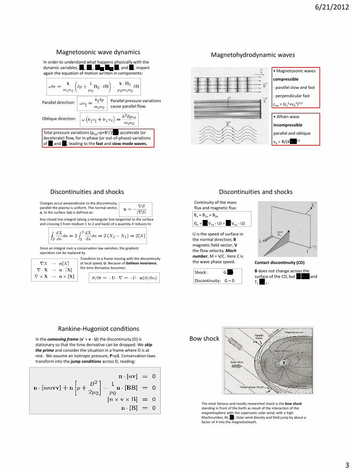
6/21/2012
3
Magnetosonic wave dynamics
In order to understand what happens physically with the
dynamic variables, vx, Bx, B , v , p, and n, inspect
again the equation of motion written in components:
Parallel direction: Parallel pressure variations
cause parallel flow.
Oblique direction:
Total pressure variations (ptot=p+B2/2 0 ) accelerate (or
decelerate) flow, for in-phase (or out-of-phase) variations
of p and B, leading to the fast and slow mode waves.
Magnetohydrodynamic waves
ひ Magnetosonic waves
compressible
- parallel slow and fast
- perpendicular fast
cms = (cs2+vA
2)1/2
ひ Alfvén wave
incompressible
parallel and oblique
vA = B/(4 )1/2
Changes occur perpendicular to the discontinuity,
parallel the plasma is uniform. The normal vector,
n, to the surface S(x) is defined as:
Any closed line integral (along a rectangular box tangential to the surface
and crossing S from medium 1 to 2 and back) of a quantity X reduces to
Since an integral over a conservation law vanishes, the gradient
operation can be replaced by
Transform to a frame moving with the discontinuity
at local speed, U. Because of Galilean invariance,
the time derivative becomes:
Discontinuities and shocks Discontinuities and shocks
Contact discontinuity (CD)
B does not change across the
surface of the CD, but 1 2 and
T1 T2 .
Continuity of the mass
flux and magnetic flux:
Bn = B1n = B2n
Gn = 1(V1n - U) = 2(V2n - U)
U is the speed of surface in
the normal direction; B
magnetic field vector; V
the flow velocity. Mach
number, M = V/C. Here C is
the wave phase speed.
Shock: G 0
Discontinuity: G = 0
Rankine-Hugoniot conditions
In the comoving frame (v' = v - U) the discontinuity (D) is
stationary so that the time derivative can be dropped. We skip
the prime and consider the situation in a frame where D is at
rest. We assume an isotropic pressure, P=p1. Conservation laws
transform into the jump conditions across D, reading:
The most famous and mostly researched shock is the bow shock
standing in front of the Earth as result of the interaction of the
magnetosphere with the supersonic solar wind, with a high
Machnumber, MF 8. Solar wind density and field jump by about a
factor of 4 into the magnetosheath.
Bow shock

6/21/2012
4
Plasma Instabilities
Because of a multitude of free-energy sources in space
plasmas, a very large number of instabilities can develop.
If spatial the involved scale is:
ひ comparable to macroscopic size (bulk scale of plasma,.....)
-> macroinstability (affects plasma globally)
ひ comparable to microscopic scale (gyroradius, inertial length,...)
-> microinstability (affects plasma locally)
Theoretical treatment:
ひ macroinstability, fluid plasma theory
ひ microinstability, kinetic plasma theory
Concept of instability
Generation of instability is the general way of redistributing
energy which was accumulated in a non-equilibrium state.
stable linear unstable metastable non-linear unstable
Linear instability The concept of linear instability arises from the consideration of
a linear wave function. Assume any variable (density, magnetic
field, etc.) here denoted by A, the fluctuation of which is A, that
can be Fourier decomposed as
In general the dispersion relation (DR) has complex solutions: =
r + . For real frequency the disturbances are oscillating waves.
For complex solutions the sign of decides whether the
amplitude A growths ( >0) or decays ( <0).
Buneman instability
The electron-ion two-stream instability, Buneman instability,
arises from a DR that can be written as (with ions at rest and
electrons at speed v0): => Current disruption
Rayleigh-Taylor instability
Consider a distortion of the boundary so the plasma density makes a
sinusoidal excursion. The gravitational field causes an ion drift and
current in the negative y direction, viy = -mig/(eB0), in which electrons
do not participate; -> charge separation electric field Ey evolves.
Opposing drifts amplify the original distortions. The bubbles develop
similar distortions on even smaller scales.
Kelvin-Helmholtz instability
Consider shear flows (e.g., due to the solar wind) at a
boundary, such as between E;ヴデエけゲ magnetosheath and
magnetopause. Linear perturbation analysis in both regions
shows that incompressible waves confined to the interface can
be excited.
ひ Shear flow at magnetised plasma boundary may
cause ripples on the surface that can grow
ひ The rigidity of the field provides the dominant
restoring force

6/21/2012
5
Firehose instability
Mechanism of the firehose
instability: Whenever the flux
tube is slightly bent, the plasma
exerts an outward centrifugal force
(curvature radius, R), that tends to
enhance the initial bending. The
gradient force due to magnetic
stresses and thermal pressure
resists the centrifugal force.
The resulting instability condition for breaking equilibrium is:
Flux tube instabilities
Current disruption
Bending of
magnetic field line
Spiral formation of
thin flux tube
Landau Damping (Lev Landau
1908-1968, Nobel prize 1962)
• Particles slightly slower than the wave gain energy
from the wave (and wave looses energy)
• Particles slightly faster than the wave loose energy.
• For a Maxwell distribution there are more slower
particles => Wave becomes damped (Landau damping)
Source: Wikipedia
Landau-damping
• Landau damping can be compared with a surfer.
• Left: Slow surfer gets catched by the wave and
gains energy.
• Right: Fast surfer catches the wave and gives
energy to the wave.
Source: Wikipedia
Waves, shocks and instabilities
• Wave occur naturally in fluid and kinetic models, e.g. Alfven waves and magnetosonic waves.
• Shocks are a special case of discontinuieties in fluid model with mass flux across the shock.
• Discontinuities happen in the fluid model, not in nature and for studying the physics of the discontinuity accurately, one has to apply kinetic models.
• Waves with growing amplitudes lead to instabilities, both in kinetic and fluid picture.
• A ゲヮWIキ;ノ キミゲデ;Hキノキデ┞ けマ;ェミWデキI ヴWIラミミWIデキラミげ ┘キノノ be treated in the next lecture.
Exercises for Space Plasma Physics:
VIII. Waves, Shocks and instabilities
1. How does an electro magnetic wave travel in vacuum and in plasma?
2. What is the cut-off-frequency? How can it be used the derive the(electron) density of a plasma?
3. If one observes the Sun in visible light and long radio waves, will the sun(visible radius) look larger, smaller or the same in radio wavelength?
4. Discuss briefly the difference between a sound wave in a neutral gasand slow/fast magnet-sonic waves and Alfven waves in plasmas.
5. What is Landau damping?
6. What are macro and micro-instabilities?
7. Why are thin current sheets important for the dynamics of space plas-mas?

7/5/2012
1
Physical Processes
8. Plasma Waves, instabilities and shocks
9. Magnetic Reconnection
Applications
10. Planetary Magnetospheres
11. Solar activity
12. Transport Processes in Plasmas
Space Plasma Physics Thomas Wiegelmann, 2012
Assuming the plasma streams at bulk
speed V, then the induction equation
can be written in simple dimensional
form as:
Magnetic reconnection
Field line merging and reconnection in the
E;ヴデエけゲ マ;ェミWデラゲヮエWヴW
magnetopaus
e
magnetotail
How to model magnetic reconnection?
• In ideal MHD, plasma is frozen into the magnetic
field => field line topology conservation and
magnetic reconnection is not possible.
• Resistive MHD in 2D
• Resistive MHD in 3D
• Collisionless reconnection, kinetic treatment
• Hybrid models, e.g. treat the ions with a kinetic
model and electrons as fluid.
Magnetic reconnection, 2D MHD
• Kinematic approach (not to be confused with kinetic
theory !!): One studies the induction equation and
ignores the equation of motion for simplicity:
• We derived this equation in exercises earlier from
Ohms law:
• In most space plasmas the Reynolds number is very
large and resistive effects can be neglected.
Source: Priest et al. JGR 108, A7, 2003

7/5/2012
2
• An exception are strong current concentrations
with high gradients in the magnetic field. Here
resistive effects become important and magnetic
reconnection can occur.
• In generally we can describe the motion of magnetic
flux, if a flux-conserving velocity w exists:
• How is flux-conserving velocity w related to
the plasma flow velocity v?
Magnetic reconnection, 2D MHD Magnetic reconnection, 2D MHD
Breaking and rejoining of two flux tubes in 2-D to form two new
flux tubes. Outside the diffusion region the flux-conserving
velocity is identical with the plasma velocity.
Source: Priest et al. 2003
Magnetic reconnection, 2D MHD
Inside the diffusion region these two velocities are NOT
identical, because the plasma is not frozen in the magnetic field
here. Source: Priest et al. 2003
Properties of 2D MHD-reconnection
• A differentiable flux tube velocity w exists
everywhere except at null points. The magnetic flux
moves at the velocity w and slips through the
plasma, which moves at v.
• Mapping of field lines are discontinuous
Moving over the
separatrix from A_1
to A_2, there is
a jump from B_1
to D_2
=> field lines break
Source: Priest et al. 2003
Properties of 2D MHD-reconnection
• Field lines preserve their connections in the diffusion
region. The exception is the X-point, where the field
lines break and their connections change.
• Reconnecting flux tubes join perfectly and outside
the diffusion region v=w.
• For a flux tube partly in the diffusion region, the
part of the flux tube in the zone slips through
the plasma. (Outside: frozen in)
• Different models have been suggested for 2D
reconnection, which based on details of
reconnection zone (e.g. Sweet-Parker model,
Petschek reconnection)
Source: Priest et al. 2003
Sweet Parker 2D-model

7/5/2012
3
• Reconnection is described as diffusion on scales
smaller than typical macroscopic scales.
• Properties in the inflow region (flow velocity,
magnetic field strength, convection electric field) are
related to the outflow
region and allow to calculate the reconnection rate
(amount of flux reconnected per time, ratio of in and
outflow velocity)
• Reconnection rate is much slower as observed in
space plasmas, but faster than global diffusion.
2D MHD-reconnection, Sweet Parker (1956)
.
Source: Wikipedia
• The reconnection rate in the Sweet-Parker
model is too slow.
• Aspect-ratio of current sheet has to
be large for high Lundquist numbers
because of the relation
• Petschek refined the Sweet-Parker model
in 1964. In and out-flow regions are separated
by slow mode shocks.
• Reconnection does hardly depend on aspect ratio
and fast reconnection is possible:
2D MHD-reconnection, Petschek model (1964)
Source: Wikipedia
Magnetic reconnection: energy conversion
• From the resistive MHD-simulations we derive
equations for the balance of mechanical and
electromagnetic energy:
• For magnetic reconnection j and E have the same
sign (why? Think about it in exercise)
=> Electromagnetic energy decreases
Thermic and kinetic energy increases
Source: Schindler & Hornig, 2001
Magnetic Reconnection, in Encyclopedia of Astronomy and Astrophysics
Time dependent reconnection
• Sweet-Parker and Petschek models investigated
stationary reconnection.
• In Space plasmas reconnection happens often
spontaneously as an instability process.
Unperturbed
1D-Harris sheet
Linear tearing
instability leads
to formation of
a plasmoid.
Source: Schindler
& Hornig, 2001
Time dependent reconnection
Source: Schindler & Hornig, 2001
Streched configurations (modified Harris-sheet) are often used as
models for the magnetotail and coronal helmet streamers. Time
dependent reconnection occur in models for substorms and
coronal mass ejections.
• Some concepts on 2D-reconnection cannot be
generalized to the 3D-case.
• Reconnection at an X-point (magnetic null) becomes
structual unstable in 3D:
- 2D X-point becomes an x-line in 3D.
-We can add a magnetic field parallel to this line
(perpendicular to 2D reconnection-plane) and
the x-line is NOT a magnetic null anymore.
• One cannot generally find a flux-conserving velocity
w in 3D. (Proof by Priest et al. 2003, omitted here)
Magnetic reconnection, 3D MHD
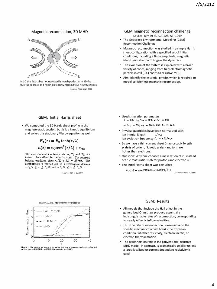
7/5/2012
4
Magnetic reconnection, 3D MHD
In 3D the flux-tubes not necessarily match perfectly. In 3D the
flux-tubes break and rejoin only partly forming four new flux tubes.
Source: Priest et al. 2003
GEM magnetic reconnection challenge Source: Birn et al. JGR 106, A3, 1999
• The Geospace Environmental Modeling (GEM)
Reconnection Challenge.
• Magnetic reconnection was studied in a simple Harris
sheet configuration with a specified set of initial
conditions, including a finite amplitude, magnetic
island perturbation to trigger the dynamics.
• The evolution of the system is explored with a broad
variety of codes, ranging from fully electromagnetic
particle in cell (PIC) codes to resistive MHD.
• Aim: Identify the essential physics which is required to
model collisionless magnetic reconnection.
GEM: Initial Harris sheet
• We computed the 1D Harris sheet profile in the
magneto-static section, but it is a kinetic equilibrium
and solves the stationary Vlasov equation as well.
Source: Birn et al. 1999
• Used simulation parameters
• Physical quantities have been normalized with
ion inertial length
ion cyclotron frequency
• So we have a thin current sheet (macroscopic length
scale is of order of kinetic scales) and ions are
hotter than electrons.
• Question: Why one chooses a mass ration of 25 instead
of true mass ratio 1836 for protons and electrons?
• The initial Harris-sheet was perturbed:
Source: Birn et al. 1999
• All models that include the Hall effect in the
generalized Ohm's law produce essentially
indistinguishable rates of reconnection, corresponding
to nearly Alfvenic inflow velocities.
• Thus the rate of reconnection is insensitive to the
specific mechanism which breaks the frozen-in
condition, whether resistivity, electron inertia, or
electron thermal motion.
• The reconnection rate in the conventional resistive
MHD model, in contrast, is dramatically smaller unless
a large localized or current dependent resistivity is
used.
GEM: Results

7/5/2012
5
GEM: Results
• RWマWマHWヴ デエW ェWミWヴ;ノキ┣WS Oエマげゲ ノ;┘ from our MHD-lecture:
• The Hall term takes care about different motion of electrons and ions.
• Please note that in kinetic (PIC or Vlasov code) we Sラ ミラデ エ;┗W ;ミ Oエマげゲ ノ;┘が H┌デ デエキゲ ノ;┘ ┘;ゲ SWヴキ┗WS in the fluid picture by substraction the momentum equations for ions and electrons.
• => Effect is naturally there in kinetic theory.
Hall term
The diffusion region
• As pointed out by Biskamp (Book:Nonlinear MHD 1993)
the diffusion region is not treated correctly in Petschek-
like-MHD-models)
• => Kinetic treatment necessary
Source: Hesse et al.
Space Sci Rev 2011
• Plasma pressure (electron pressure tensor) is not isotrop
and not even gyrotropic in diffusion region.
• Simulations with mass ratio m_i/m_e=256, Hesse et al
Source: Hesse
et al. 2011
Reduced distribution F(vx, vy ) in the outflow region. The
distribution demonstrates the preferential loss of accelerated
particles from the dissipation region. Source: Hesse et al. 2011
• Electrons become unmagnetized in diffusion region.
• Schematic picture of meandering electron orbits in a
magnetic field reversal.
Source: Hesse et al. 2011 Source: Hesse et al. 2011

7/5/2012
6
Magnetic reconnection
• Magnetic reconnection changes the magnetic field
topology and magnetic energy is converted into
thermal and kinetic energy.
• Reconnection was studied first in 2D resistive MHD
with stationary and time-dependent models.
• In ideal MHD magnetic reconnection cannot happen.
• In the resistive (or diffusive) zone, basic assumptions
of MHD break down and kinetic effects become
important.
• Reconnection in 3D can happen at 3D-magnetic-Nulls
and also for non-vanishing magnetic fields
(active area of research and details are outside of
scope of this indroductory lecture)

Exercises for Space Plasma Physics:
IX. Magnetic Reconnection
1. What is magnetic reconnection?
2. Where in the solar system is magnetic reconnection important?
3. Can reconnection happen in laboratory plasmas?
4. Why does the current density j and the electric field E have the samesign in magnetic reconnection? Hint: study the 2D-case and applyOhm’s law at the X-point.
5. How is magnetic energy converted to other energy forms (which one)during magnetic reconnection?
6. Any idea why scientist use a reduced mass ration mi/me of 25, 256 etc.for Vlasov-code or full particle simulations instead of the correct value1836 for a proton electron plasma ?
7. Which MHD-assumptions break down in the diffusion zone?

7/6/2012
1
Physical Processes
8. Plasma Waves, instabilities and shocks
9. Magnetic Reconnection
Applications
10. Planetary Magnetospheres
11. Solar activity
12. Transport Processes in Plasmas
Space Plasma Physics Thomas Wiegelmann, 2012
Earth magnetosphere
Magnetospheric substorm
Substorm phases:
ひ Growth
ひ Onset and expansion
ひ Recovery
Show movie:
http://www.youtube.com/watch?v=BDZj1CmsJ64
Growth phase of magnetotail
• The growth phase (quiet evolution of magnetotail before a substorm) can be modelled as a sequence of magneto-static equilibria.
• Magnetic pressure in the lobe changes slowly (solar wind compresses field lines) and remains in equilibrium with plasma pressure in the plasma sheet.
• The magnetic field topology does not change in this phase (ideal MHD, no resistivity).
• Sequence of equilibria are not independent and the ideal MHD-evolution has to be implemented in the model.
Magnetospheric convection in quiet states (Source: Schindler & Birn, JGR 1982)
Noon-midnight meridian plane of the magnetosphere.
V(A) is proportional to the differential volume
between field lines A and A + dA.
Ideal MHD
Ideal Ohms Law
Equation of state,
Adiabatic convection
Continuity Eq.
Force-balance
Maxwell
Source: Schindler & Birn, JGR 1982
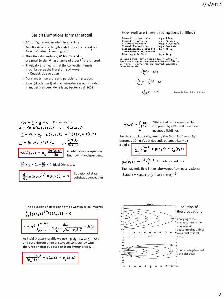
7/6/2012
2
Basic assumptions for magnetotail
• 2D configuration, invariant in y, no B_y
• Tail-like structure, length scale L_x >> L_z.
Terms of order are neglected.
• Slow time dependence,
are small (order ) and terms of order are ignored.
• Physically this means that the convection time is
much larger as the travel time of waves.
=> Quasistatic evolution
• Constant temperature and particle conservation.
• Inner (dipolar part) of magnetosphere is not included
in model (Has been done later, Becker et al. 2001)
How well are these assumptions fulfilled?
Source: Schindler & Birn, JGR 1982
Grad-Shafranov equation,
but now time-dependent.
Ideal Ohms Law
Force-balance
Equation of state,
Adiabatic convection
Differential flux volume can be
computed by differentiation along
magnetic fieldlines.
For the stretched tail geometry the Grad-Shafranov-Eq.
becomes 1D (in z), but depends parametrically on
x and t.
The magnetic field in the lobe we get from observations:
Boundary condition
The equation of state can now be written as an integral:
As intial pressure profile we use
and sove the equation of state selfconsistently with
the Grad-Shafranov equation (usually numerically).
Solution of
these equations
Changing of the
magnetic field in the
magnetotail.
Sequence of equilibria
constraint by ideal
MHD.
Source: Wiegelmann &
Schindler 1995

7/6/2012
3
Formation of thin current sheets
• Within our model assumptions strong current
concentrations (thin current sheets) form.
• Such configurations are prone to current driven
micro-instabilities (kinetic instabilities).
• Micro-instabilities cause resistivity on macroscopic
MHD-scales.
• The assumption of ideal MHD is violated and
we need (at least) use resistive MHD for further
investigations.
• => Topology changes by magnetic reconnection and
a fast dynamic evolution is possible (not quasistatic
anymore) => Eruption phase of substorms start.
Formation of thin current sheets
Resistive magnetotail MHD-simulations (Otto et al. 1990, JGR)
Source: Otto et al. 1990, JG
Thin current sheets
• We can understand the formation of strong current
concentrations within MHD.
• Spatial scales in thin current sheets become very
small and comparable with ion gyro-radius
(about 500 km in magnetotail).
• => A basic assumption of MHD is violated and we
need to apply kinetic theory (Vlasov equation).
• Stationary Vlasov equilibria.
• Time dependent evolution (either solve Vlasov-eq.
directly or indirectly by particle in cell simulations.)
Vlasov-Maxwell Equations kinetic description of a collisionless plasma

7/6/2012
4
• Vlasov Equation conserves particles
• Distribution functions remains positive
• Vlasov equation has many equilibrium solutions
Properties of Vlasov Equation
=> Proof see Lecture 4, Kinetic Theory
• Constants of motion (2D, x,z):
- momentum in y
- Hamiltonian
• Stationary solution of Vlasov equation:
• Macroscopic quantities (charge and current density)
we get by integration over velocity space:
Thin current sheets, Kinetic theory Source: Schindler&Birn, JGR 2002
• Inserting into Maxwell equations:
• Using the quasi-neutrality condition
we can eliminate the electro-static potential and
derive the Grad-Shafranov equation (like in MHS):
• Plasma pressure is isotropic (in x,z) for
these form of distribution functions:
Thin current sheets, Kinetic theory
• Remember that any distribution function depending
only on constants of motions solves the stationary
Vlasov equation. Examles used in (Schindler & Birn 2002):
• LTE => Local Maxwellian of Hamiltonian:
• The momentum in y causes electric currents (ions
and electrons move in opposite direction, but the currents
in the same. P_y profile can be derived from the
result of sequences of magneto-static equlibria.
• Please note that this still leads to some freedom in
the distribution functions, e.g. different temperatures
for ions and electrons, thickness of sheet can be used.
Thin current sheets, Kinetic theory
• Dimensionless parameters:
• Remember: MHD is valid only if spatial dimension L is much larger as the gyroradius. As larger this ratio, as more important are kinetic effects.
Thin current sheets, Kinetic theory
Ratio of ion-gyro-radius to
spatial dimension L of the
current sheet.
Pictures from Schindler
& Birn, JGR 2002
Electron current
becomes more
important if spatial
dimensions
comparable with
ion-gyro-radius

7/6/2012
5
Thin current sheets, Kinetic theory
As in MHD, A(x,z) defines the magnetic field lines and
the relation A-> J_y can be used to compute
J_y(x,z). (Picture from Schindler & Birn, JGR 2002) Pictures from Schindler
& Birn, JGR 2002
Thin current sheets,
Kinetic theory
• j_ad corresponds to
MHD case (gyro-radius
infinitesimal small)
• Taking finite gyroradius
effects into account
localises the sheet in x,
but smears it out in z.
• Ouside the current sheet,
MHD is valid and
the configurations are
the same.
Magnetosphere
• We can understand the growth phase of a substorm
as a sequence of magneto-static equilibria.
• Interaction with the solar wind leads to stretching
of the magnetotail and formation of thin current
sheets in the center of the plasma-sheet.
• Thin current sheets cause resistivity on MHD-scales
and lead to magnetic reconnection and initiation
of the dynamic phase of a substorm.
• This eruptive phase can be simulated with time-
dependent, resistive MHD-simulations.
• In the thin current sheets itself the MHD-approach is
not valid and we need to apply a kinetic model.

Exercises for Space Plasma Physics:
X. Magnetosphere
1. How can the full MHD-equations be simplified to describe the quiet
loading phase before a magnetic storm occurs?
2. Explain the physical processes which occur, when the slow quasistatic
evolution of the magnetotail ends and a very dynamic eruptive phase
starts.
3. Resistivity is a kind of friction in a plasma. How can it be that such
kind of friction plays a key-role for the initiation of dynamic processes?
For comparison: in classical mechanics friction slows down the motion
of say a pendulum, but does not initiate the motion. How can it be
that an ideal plasma remains calm, but erupts when resistivity occurs?
4. In the lecture we derived the Grad-Shafranov equation from magneto-
hydro-statics. How can one find corresponding distribution functions
which fulfill the stationary Vlasov-equation?
5. Scientists apply both MHD-models and kinetic models to study mag-
netospheric physics. Is this necessary? If MHD is not sufficient to
understand some physical processes, why not study the whole magne-
tosphere with a kinetic model?
6. How could one in principle model planetary magnetospheres, like,e.g.,
the Jovian magnetosphere where fast planetary rotation and mass load-
ing from the moon Io is assumed to play an important role?

7/12/2012
1
Physical Processes
8. Plasma Waves, instabilities and shocks
9. Magnetic Reconnection
Applications
10. Planetary Magnetospheres
11. Solar activity
12. Transport Processes in Plasmas
Space Plasma Physics Thomas Wiegelmann, 2012
Solar activity
is driven by
magnetic
fields!
Corona of the active sun, SDO (Solar
Dynamics Observatory), Jan. 2012 Plasma loops in solar corona, SDO, Jan. 2012
Solar Eruptions
• The solar coronal plasma is frozen into
the coronal magnetic field and plasma
outlines the magnetic field lines.
• Coronal configurations are most of the time
quasistatic and change only slowly.
• Occasionally the configurations become unstable and
develop dynamically fast in time,
e.g., in coronal mass ejections and flares.

7/12/2012
2
Lorentz force
pressure gradient
gravity
How to model the stationary Corona?
Force-free Fields
Low plasma Beta in corona
Neglect plasma pressure+gravity
Force-Free Fields
Equivalent
• Potential Fields (no currents) • Linear force-free fields
(currents globally proportional to B-field)
Relation between currents and magnetic field. Force-free functions is constant along field lines, but varies between field lines. => nonlinear force-free fields
Further simplifications
Here: global constant linear force-free parameter
Global potential Field Bochum, 04.02.2010 10 Coronal Plasma seen in EUV.
A subclass of force-free fields are current-free
potential fields.
Nonlinear Force-Free Fields
• For equilibria with symmetry we can reduce the force-free equations to a Grad-Shafranov equation (Low&Lou 1990).
• In 3D, the NLFFF-equations are solved numerically. • Suitable boundary conditions are derived from
measurements of the photospheric field vector. - Bn and Jn for positive or negative polarity on boundary (Grad-Rubin) - Magnetic field vector Bx By Bz on boundary (Magnetofrictional, Optimization)
Equivalent
Nonlinear force-free fields in 2.5D (Source: Low&Lou, ApJ 1990)
• In spherical geometry (invariant in phi, but B-field has 3 components) the magnetic field can be represented as:
• The force-free equations reduce to a Grad-Shafranov Eq.:
• Low&Lou 1990 found separable solutions: a and n are free parameters.

7/12/2012
3
Nonlinear force-free fields in 2.5D
The angular functions P are computed by solving an ordinary (but nonlinear) differential equation. This can be easily done, e.g. with a Runge-Kutta method.
Nonlinear force-free field in spherical geometry with symmetry in phi.
(Source: Low&Lou 90)
Nonlinear force-free fields in 2.5D => 3D looking fields in cartesian coordinates
A nice property of these equilibria is, that one get 3D-looking configurations by shifting and rotating geometry. => Model for a solar Active Region.
(Source: Low&Lou 90)
Low&Lou-model active regions, PHI was varied
Bochum, 04.02.2010 Das Magnetfeld der Sonnenkorona 16
Some properties for force-free fields in 3D
(Molodensky 1969, Aly 1989)
Boundary flux balanced
Maxwell Stress
torque
No net force on boundaries
No net torque on boundaries
Force-Free
B-Field Measurements, non-force-free
MHD-relaxation Chodura & Schlueter 1981
Optimization Wheatland et al. 2000

7/12/2012
4
Nonlinear force-free coronal magnetic fields extrapolated with optimization method from SDO measurements. Selected field lines are colour coded by the amount of electric current they contain. 5h after this snapshot a X-class (large!) Flare occured. Source:Sun et al., ApJ 2012
Nonlinear force-free fields in 3D
Monitoring of free magnetic energy before and after the X-class Flare (dotted vertical line) by a sequence of force-free equilibria. During the Flare magnetic energy is converted to thermal and kinetic energy => Dynamic phase, cannot be modelled by sequences of equilibria. Source:Sun et al., 2012
Time dependent evolution of force-free fields
In the limit of a vanishing plasma beta the ideal, time dependent MHD-equations are:
Nonlinear force-free equilibria contain free energy and can become unstable, e.g. an ideal kink-instability. Source: Kliem and Török, ESASP 2004
Time dependent
evolution of force-
free fields
Left: Confined filament
eruption observed with
Trace in May 2002.
Right: Magnetic field lines
of a kink-unstable flux robe.
Source: Kliem&Török, ApJL 2005
Movies: http://www.lesia.obspm.fr/perso/tibor-torok/res.html
Coronal plasma and magnetic field
Lorentz force
pressure gradient
gravity
B
for vertical scales < 0.1 RS
(gravitational scale height) => Pressure constant on field lines
Newark, 31.03.2008 24
Force-free equilibria and coronal plasma
small small

7/12/2012
5
Coronal plasma loop modelling
• The magnetic field structures the solar corona and
due to the low plasma-beta we can neglect plasma
effects when modelling the coronal magnetic field.
• Modeling the coronal plasma can be done with
1D-hydrodynamics models along the magnetic field
lines. (Question/Exercise: Why not MHD along loops?)
• Time-dependent processes (like reconnection) are
thought to be important for heating (and flares,
eruptions etc.)
• Here we concentrate on stationary solution.
1D plasma loop modelling Source: Aschwanden&Schrijver, ApJ 2002
Continuity Equation
Momentum Eq.
A is the loop cross section and s a coordinate along the loop.
Energy Eq. conduction heating radiative
cooling
Source: Aschwanden&Schrijver 2002
conductive flux
heating rate, not very well
known, E_0 is heating at base
radiative cooling, proportional
to square of electron density
and a factor (Temperature
dependent, not well known)
Analytic approx. of the numerical solution
Source: Aschwanden&Schrijver 2002
Computing the numerical solution is
expensive and analytic approximations
useful. (L is loop half-length, a and b
are fitting parameters.)
Scaling laws • Analytic expression help to compute the plasma
along many field lines, which is numerically very expensive. Plasma pressure can be derived by integration.
• Analytic models are simplifications, based on circular loops and static equilibria without flow.
• In a subsequent work Schrijver et al. 2005 derived scaling laws and related the heating flux density to magnetic field strength at loop base B_base and loop half length L:
• Best agreement was found (in CGS-units) for:
Top: coronal plasma from Yokoh/SXT
Bottom: Scaling law model
The coronal
plasma model
in the bottom
images is
based on a
potential
field model
for the
magnetic
field and
scaling laws
for the plasma.
(Source:
Schrijver
et al. 2005)
Dec. 1, 2000 Dec. 8, 2000

7/12/2012
6
Time-dependent MHD-simulations
Self-consistent equilibrium
Artificial images
LOS-integration
Coronal plasma modeling
Where to go?
Force-free code
Vector magnetogram
MHS code
3D Force-free magnetic field
3D field lines
com
par
e
Plasma along magnetic
loops
Scaling laws
Stereoscopy STEREO images
3D EUV loops
consistent?
Summary: coronal plasma
• Due to the low plasma-beta in the solar corona the coronal magnetic field is force-free.
• With nonlinear force-free models we can monitor the total and free energy of active regions.
• Configurations with free energy can become unstable and erupt => Flares, mass ejections.
• Eruptive phase can be modelled with time-dependent MHD-simulations.
• Coronal plasma is frozen into the magnetic field and can be modelled by 1D hydrodynamics along the magnetic field lines.

Exercises for Space Plasma Physics:
XI. Solar Corona
1. Why is the solar magnetic field important for the structure and dy-namics of the solar corona?
2. How can the MHD-equations be simplified to study the evolution ofthe solar corona in quiet and active times?
3. The solar corona is much hotter as the solar surface. How can thishappen. Our normal life experience tells us that it becomes colder asfarer one moves away from a heat source.
4. What is the difference between an ideal and resistive MHD-instability?
5. If plasma and magnetic field (plasmoids) are ejected in a coronal massejection, magnetic reconnection must occur at some point. Why? It isnot entirely clear, however, if reconnection is the driver of the eruptionor just occurs in the aftermath. Describe briefly both scenarios.
6. Is the heat conduction parallel and perpendicular to magnetic loopsthe same or different?
7. What are scaling laws and are they useful?

7/19/2012
1
Physical Processes
8. Plasma Waves, instabilities and shocks
9. Magnetic Reconnection
Applications
10. Planetary Magnetospheres
11. Solar activity
12. Transport Processes in Plasmas
Space Plasma Physics Thomas Wiegelmann, 2012
Transport in neutral gases
• Transport processes in gases have first been studied
by Maxwell and Boltzmann, the founders of kinetic theory.
• Aim of transport theory is to understand non-equilibrium
processes from first principles.
• For neutral gases this approach was successful in, e.g.,
pridicting of transport coefficients like:
- diffusion
- heat conduction
- viscosity
-thermo-diffusion (cross-coefficients for different species)
• Motor for irreversibility are (mainly binary) collisions.
Transport in plasmas
• Theory was driven mainly to understand fully ionized
plasmas in fusion experiments (since mid 20th century)
• Naturally scientists applied the well known methods
from gas-kinetic-theory to plasmas.
• But there are two major differences
1.) Plasma contains charged particles and (long-ranging)
Coulomb interaction dominate interaction of particles.
2.) External electric and magnetic fields act on the
charged particle.
Classical transport theory in plasmas
• A formalism (Chapman-Enskog theory for multicomponent
gases) treats non-equilibrium gases as (small)
perturbations from Maxwell-Boltzmann distribution.
• Incorporating electromagnetic fields, Coulomb-collisions
etc. in this formalism lead to the classical transport theory
for plasmas (Braginskii 1965, Balescu 1988)
• So far so good. But then the theory was compared
with experiments and this was really disappointing:
• Classical transport theory grossly underestimated the
transport-coefficients, often by several orders of
magnitude!!
Transport in space-plasmas
• Limitations of classical transport theory apply
also to space plasmas.
• Classical theory was succesfull to calculate transport
coefficients like conductivity (or キデけゲ inverse the resistivity)
for weakly ionized plasmas like the
ionosphere. (Spitzer resistivity)
• For fully ionized space plasmas we face the same
problem as in fusion theory: the transport coefficients
(say resistivity) are orders of magnitudes to low.
• From classical theory most space plasmas would be
ideal and resistive processes (like reconnection) would not
play any role.
Plasma resistivity in partly ionized plasma
In the presence of collisions we have to add a collision term in the
equation of motion. Assume collision partners moving at velocity u.
In a steady state collisional friction balances electric acceleration.
Assume there is no magnetic field, B = 0. Then we get for the electrons
with ions at rest:
Since electrons move with respect to the ions, they carry the current
density, j = -eneve. Combining this with the above equation yields, E =
j, with the resistivity:

7/19/2012
2
Conductivity in a magnetized plasma In a steady state collisional friction balances the
Lorentz force. Assume the ions are at rest, vi = 0.
Then we get for the electron bulk velocity:
Assume for simplicity that, B=Bez.
Then we can solve for the electron
bulk velocity and obtain the current
density, which can in components be
written as:
The current can be expressed in the form of Oエマけゲ
law in vector notation as: j = E, with the dyadic
conductivity tensor .
Conductivity in a magnetized plasma
For a magnetic field in z
direction the conductivity
tensor reads:
The tensor elements are the
Pedersen,D, the Hall,H, and the
parallel conductivity. In a weak
magnetic field the Hall conductivity
is small and the tensor diagonal, i.e.
the current is then directed along
the electric field.
Successful method for weakly ionized plasmas like inosphere
Which assumptions of classical transport
theory are invalid in fully ionized plasma?
• 1.) Collisions cannot be considered as binary
interactions due to the long ranging Coulomb force.
• => For weakly non-ideal (fusion) plasma this problem
was treated by the Lenard-Balescu equation, which
takes the many-particle character of Coulomb
collisions (Debye-Shielding) into account.
• 2.) Influence of external magnetic fields on the
free motion of particles in fusion devices (toroidal
magnetic field and space plasmas.
• => Gyration, Drifts etc. which we studies in test-
particle approach. But these effects have large
influence on computing transport coefficients.
A Tokamak contains
strong magnetic fields
in a toroidal geometry in
order to trap plasma for
nuclear fusion.
But as we just learned:
transport coefficients have
been underestimated by
orders of magnetide
Plasma transported
away and not trapped
long enough for fusion
Tokamak
Neo-classical transport theory
• Strong and inhomogenous magnetic fields occur
both in tokamaks (fusion machines) and space plasmas.
• Effect of these strong magnetic fields has been first
investigated for toroidal magnetic fields. This research
was clearly dedicated for fusion plasmas.
• Combining the effects of strong magnetic fields with
methods of classical plasma transport lead to
significantly higher transport coefficients.
• The new approach was dubbed neo-classical
transport theory. (Galeev&Sgdeec 1968,
Hinton & Hazeltine 1976, Balescu 1988)
Neo-classical transport theory
• Neo-classic theory was an important step forward in
fusion theory (never become that popular for space
plasmas) and showed reasonable agreement with some
experiments.
• But: Still not satisfactory to explain the often observed
leaks in tokamaks.
• Problem: A real plasma is never in a quiescent state
(like the static and stationary equilibria we calculated)
but collective nature of plasma dominates キデけゲ behaviour.
• At high temperatures (both in fusion and space plasmas)
particle collisions are less important than self-organized
effects like waves, vortices, modes etc.

7/19/2012
3
Collective effects
• Such self-organized coherent structures are more
efficients to tranport plasma and energy than interaction
of individual particles. (For space-plasma physicists
キデけゲ interesting to study these dynamics, but
fusion-people loose the plasma in their machines
due to these effects => no fusion.)
• Remember the many waves we studied in space plasmas
(and we studied only a small fraction of all known plasma
waves and in simplified geometries)
• Some waves become unstable (growing amplitudes)
and we studied instabilities mainly with linear theory.
• For large amplitudes nonlinear effects become important.
Complexity and turbulence
• For low aplitude waves linear superposition can
be used to study the combined effects.
• As amplitudes grow, nonlinear interactions become
very important => One gets a large number of new
modes, saturation of amplitudes.
• => The plasma becomes more and more complex
and キデけゲ behavious unpredictable.
• => Turbulent or chaotic motion.
• In chaos small differences in location and velocity
can influence significantly the evolution
(like the butterfly-effect in weather prediction).
Non-equilibrium steady state
• Under quiet condition the random collisions in
a gas lead to a steady state thermal equilibrium.
• For the Boltzmann-equation (Vlasov-equation with
Boltzmann collision term) it has been proofed that
the final stationary state solution is the Maxwell-
Boltzmann distribution for the distribution functions.
• Turbulent, collective interaction (e.g. of particles and
waves) will lead to a non-equilibrium steady state.
• Turbulent dissipation becomes very important and
does of course influence (or even dominate!) the
transport coefficients (additional to classical and neo-
classical effects)
• => Anomalous Transport Theory
Anomalous vs. strange transport
• In anomalous transport theory the transport
coefficients are computed from turbulent/chaotic
collective particle motions.
• In many cases the relations between macroscopic
plasma variables remain simple, e.g. a linear
dependence of fluxes and forces.
• One can still use fluid theory, but with transport
coefficients computed by turbulent theory.
=> Macroscopic laws are the same as in classical theory
• In some cases, however, turbulence can lead to
strange results, e.g. the transport coefficients are
either zero or infinity => strange transport.
(maybe called strange because we not understand it)
Anomalous transport: Quasi linear theory
• Quasi-linear theory, valid for weak turbulence.
• Particle distribution function and fields can be split into a
slowly evolving part ( fs0, E0, B0) and small fluctuations
(fs, E and B)
• We get the Vlasov equation for the slowly evolving part:
• As we calculated in the excercises, the entropy remains
constant in Vlasov systems. If one defines, however,
an entropy only for the slowly evolving part, this
(new defined) entropy can increase and be used to
measure the disorder of a system
Numerical simulations
• In many cases we cannot apply quasi-linear theory or
other analytic methods and use numerical simulations.
• Are simulations theory or experiments?
• For experimental physicists (or observers in space
physics) often everything not related to experiments
or observations is theory.
• But: Often not true and we speak of so called:
numerical experiments. Simulations produces often
such huge amount of data, that methods similar as for
observational data are used to analyze them.
• If we able to correctly simulate a physical system, this
does not necessarily mean that we understand all physics.
(But it helps, as we can switch on/off physical terms.)

7/19/2012
4
Magnetic Helicity
• Magnetic helicity is a measure on the complexity of magnetic fields.
• Helicity is conserved for ideal MHD-processes and also for some resistive processes like 2D reconnection.
• For 3D reconnection, the helicity can change, but is dissipated much slower as the energy.
• Approximate helicity conservation constrains (additional to energy conservation) which physical processes are possible.
• E.g., A nonlinear force-free magnetic field cannot relax to a potential-field (which would have zero helicity), but only to a linear force-free field with same helicity. (Or the helicity must be transported away, e.g. by a coronal mass ejection).

7/19/2012
5
Fluid vs. Vlasov approach
• In Vlasov theory we study distribution functions
f(x,v,t) in 6D-phase space.
• In Fluid equations we deal with macroscopic plasma
variables like density n(x,t), flow velocity, V(x,t),
plasma pressure p(x,t) in the 3D configuration space.
• What is gained and lost by these approaches?
• The fluid equations are simpler and easier to solve.
• The Vlasov approach is more complete and includes
the microphysics.
Fluid vs. Vlasov approach
What is gained by fluid approach?
• It is easy to extend the fluid equations to include
collisions, e.g. momentum transfer between ions
and electrons or also the inclusion of neural gas
atoms. (Computing a collision term in kinetic theory
is much more complicated, in particular for anomalous
transport)
• One can simplify the fluid equations further by
reasonable (for studied system) assumption, e.g. using
a scalar pressure instead of tensor or neglection the
pressure for low-Beta force-free fields.
Fluid vs. Vlasov approach
What is lost in the fluid approach?
• Fluid equations are not closed (momentum hierarchy)
=> We have more variables than equations.
• Often it is not easy, however, to make assumptions for
pressure, equation of state or energy equation.
• If we can solve f(x,v,t) from Vlasov theory however,
computing the pressure tensor and higher moments
is just a simple integration => One can deduce an
equation of state from Vlasov theory.
• Microphysics effects are lost in fluid theory, in
particular all effects in velocity space like Landau
damping and kinetic instabilities.
What is missing in Vlasov theory?
• Vlasov equation is basically a fluid flow in 6D-phase-space
• Not included in Vlasov theory are all effects, where the discreteness of the plasma (that plasma is a collection of individual particles) is important:
• What is the level of electromagnetic fluctuations in a stable plasma?
• What is the emission rate and spectrum of radiation from a plasma?
• What is the cross section for scattering of radiation from a plasma?
• => Need higher order kinetic equations.

�������������� ������ �����������������������
�������������
� �� ���������������������������� �� ���������������������������� �� ��� ������������� ���� ��� ������������� ���� ��� ������������ ������������������ ��� �� ���������� � �������� �� !� ∀���#������ �� ∃ ������������������� ������ ∀�%������� �� ∃ �������������������� �� ��∀ �����&�∀ �������� � ��∀�� �� ∋� ���%� �� �(�� �� ���������#����� �� �� ������ �� ����������������������)%����∗�� �� +����,��������������� �� �� ������#�����−�∋��������� � ��∀�� �� &������� �