Space weather prediction via complexity measures in the solar-terrestrial record J. A. Wanliss, Michael Watke, Thomas Bitner, James Johnson, Ali Knaak Presbyterian College 503 S. Broad Street Clinton, SC, 29325 USA P. Dobias DRDC CORA 101 Colonel By Dr. Ottawa, ON Canada Abstract In this paper we present evidence that the magnetosphere-ionosphere system is always in a critical state. This idea has been previously considered for magnetospheric substorms, but here we present evidence that even global space storms feature self-similarity and scaling behavior. Whereas prior to the onset of the space storm the nonlinear scaling exponent was varying only slowly and continuously, reminiscent of a second order type phase transition from one critical state to the next, the onset of the storm resulted in a dramatic change such as might result from a dynamical instability characterized by a first-order-like topological phase transition.

1. Introduction Space storms characterize the most dynamic plasma and field behaviour in the magnetosphere. Storms include a wide variety of electromagnetic processes extending from the surface of the earth into the deep magnetosphere, with the primary locus of activity in the near-earth geospace environment [Baker et al., 1997; Li et al., 1997; Reeves, 1998]. Important processes include energetic particle injection and precipitation [Horne 2003], acceleration of relativistic electrons [Li et al., 2001; Meredith et al., 2003], ring current enhancement, decay, and composition changes [Daglis et al., 1999; Liemohn et al., 2001; Kozyra et al., 2002]. Recent studies on the causes of space storms have found that coronal mass ejections and extreme values of the southward interplanetary magnetic fields appear to be key factors in storm development [Gonzalez et al., 1994; Richardson et al., 2001]. Long-range interactions between the ionosphere and magnetosphere also play an important role in the initiation and development of space storms, and interaction between these two spheres is highly nonlinear [Lui, 2002; Daglis et al., 2003 and the references therein]. Storms thus form a system of nonlinear phenomena that include components of solar and terrestrial origin [Daglis et al., 2003]. The connection between solar wind fluctuations and storms is so strong that the almost instinctive reaction of space physicists is to minimize the role of internal magnetospheric dynamics and to place virtually all the blame on the solar wind. It is therefore often considered that the problems of space weather can be solved in the main via accurate and more complete monitoring of the solar wind. In this paper we will investigate the statistical nature of the magnetosphere prior to, and during, space storms via the SYM-H index. SYM-H is different from the DST-index which is traditionally used for characterization of space storms; SYM-H uses data from different magnetometer stations, has a cadence of one-minute rather than one hour, and convolves the station data in a slightly different manner than DST. These differences notwithstanding, the two indices are effectively interchangeable in an operational sense [Wanliss and Showalter, 2005]. Recently Wanliss [2004, 2005] and Wanliss et al. [2005] analyzed the storm index SYM-H in terms of nonlinear statistical properties. They found that for extremely quiet intervals and extremely active intervals the nonlinear statistical behaviour is quite different. This is not merely a fancy way of saying that storms are different from quiet times. It says this, and more -- that the fractal scaling properties are different during these times. The significance of this has previously been recognized for the substorm, which is a smaller scale magnetospheric activity frequently related to storms. Magnetospheric substorms develop most dramatically upon disruption of the crosstail electric current; this results in rapid dipolarization of the inner magnetotail magnetic field. The period prior to dipolarization features steady stretching of the inner magnetotail and thinning of the current sheet [Kaufmann, 1987; Wanliss et al., 2000]. Ohtani et al. [1995] and Consolini and Lui [2000] examined scaling properties of magnetic fluctuations in the magnetotail, the latter finding a fractal scaling exponent 0.48 0.02 before current disruption, changing to 0.70 0.02 afterward. They concluded that the post-disruption statistics implied a persistent signal that may be the result of reorganization

during current disruption. In other words, there may be a phase transition-like behaviour of the magnetosphere during substorms [Sitnov et al., 2000]. The work of Wanliss [2005] considered quiet times separate from active times, and in the majority of cases the active times were not substorms but were full-fledged space storms. They analyzed the space storm index SYM-H for the epoch 1981-2002 and separated quiet intervals from active intervals on the basis of the Kp index. Although this is not the same situation as considered the by Ohtani et al. [1995] and Consolini and Lui [2000], Wanliss [2005] found some similarity in that active intervals generally had larger scaling exponents than the quiet intervals. This may be important because it suggests the possibility that there is a common statistical behaviour during quiet intervals that is different from the typical statistical behaviour observed during active (storm) intervals. An overall trend towards higher scaling exponents was also discovered for increasing magnetospheric activity, possibly implying an increase in organization with magnetospheric activity. The significance of a change in the scaling exponent is that it suggests a symmetry-breaking in a system in a state of self-organized criticality (SOC). This may occur when a system is perturbed near a critical point [Chang, 1992]. None of the results from the work cited above directly prove SOC, but they are consistent with SOC – they are a necessary, but not sufficient, condition for SOC. The difference in scaling exponents from quiet and active intervals seems to suggest that the magnetosphere exists in a critical configuration. This is hard to accept in the case of space storms, because as mentioned previously, these are generally understood to be a direct result of solar wind fluctuations. The classical view of storms seems to be mostly correct in that one can often link coronal mass ejections to subsequent space storms [Huttunen et al., 2002]. But if it is mostly correct that means, at the least, that there are features that cannot be sufficiently explained by traditional models. While the development and gross morphology of space storms is fairly well understood, a consensus has not been reached regarding the trigger/s of space storms. Coronal mass ejections and extreme values of the southward interplanetary magnetic fields appear to be among the leading factors in storm development, although neither of these factors by themselves are sufficient nor necessary for storm occurrence or development. For example, during solar minimum different factors seem to drive storms [Webb et al., 2001]. The solar wind is clearly the driver of storms, but the precise development and trigger mechanisms are cloudy. In this brief paper we will consider the possibility that a space storm can be modeled as a phase transition that is described by a multifractional Brownian motion (mfBm). We will present observational evidence together with a theoretical outline that supports this hypothesis. We must emphasize that we are not in any way trying to suggest that space storms are an example of SOC -- we consider this to be highly unlikely because of the driven nature of the solar-terrestrial interaction. In the context of this mfBm hypothesis one can think of the pre-storm magnetospheric state as being highly disordered, until the statistical state of the system passes through the critical point that precipitates the mostly ordered and imitative state of the space storm. The system goes critical when local influences propagate over long distances and the average state of the system becomes

exquisitely sensitive to a small perturbation; that is, different parts of the system become highly correlated. 2. Fractional and multifractional Brownian motion and methods A signal B(t) that displays fractional Brownian motion (fBm) is one for which both the real and imaginary components of the Fourier amplitudes are Gaussian-distributed random variables [Hergarten, 2002]. In addition, the mean of the Fourier amplitudes

() 0 and ()( ')* P() ( ') , where P() ~| |2 1 . This means that for the special case α=1/2, fBm reduces to the well-known random walk with a power law spectrum varying as an inverse square. Signals with scaling exponents above α=1/2 are called persistent, because if the data at some point have B(ti+1)>B(ti), for example, then the probability is greater than 0.5 that B(ti+2)>B(ti+1). Signals with exponents below 1/2 are called antipersistent because if B(ti+1)>B(ti), the probability is greater than 0.5 that B(ti+2)<B(ti+1). Typically, fBm is nonstationary, and thus detection of the presence of memory is a delicate task. Nonstationarity means that the statistical properties are not constant through the signal, and traditional analysis methods, that assume stationarity (e.g. power spectra), cannot be used. Notwithstanding the difficulties, fBm has been recognized in a variety of fields, including hydrology, geophysics, biology, telecommunication networks, and others. Figure 1 shows examples of fBm calculated from the Wood-Chan circulant method [Wood and Chan, 1994]. The roughness of the curves is greater for smaller values of the scaling exponent.

Figure 1. Examples of fBm for different values of the scaling exponent. The axes are arbitrary. Multifractional Brownian motion (mfBm) is a generalised version of fBm in which the scaling exponent is no longer a constant, but a function of the time index of the original process [Peltier and Levy Vehel, 1995]. In this case the increments of mfBm are nonstationary and the process is no longer self-similar. Figure 2 shows a simple example of a mfBm. In this example the scaling exponent does not change continuously but as a step functional parameter; it has a value 5.0 for the first half of the series and

7.0 for the rest. The abrupt transition is clear from Figure 2a because the smoothness

of the series changes suddenly in the middle of the series. An abrupt change like this is characteristic of systems that undergo a phase transition. For instance a phase transition in water (evaporation/condensation) brings about a change in long-range correlations in molecular motion. Obviously, the free Brownian motion of gas molecules is not reproducible in a fluid. In this case the motion of molecules is highly correlated due to a presence of strong intermolecular forces. Therefore, the phase transition in this case is characterized with a change in scaling parameter that characterizes correlation of molecular motion.

Figure 2. (a.) Model mfBm calculated by splicing together two fBm series with 5.0 and .7.0 The change is apparent from the smoothness change at the middle of the series. (b.) Scaling exponent )(t computed from DFA. To examine these data, shown in Figure 2a, one can study how a fluctuation measure, denoted here by ,F scales with the size n of the time window considered. Specific methods, such as Hurst’s rescaled range analysis [Hurst, 1951], power spectral analysis, structure function analysis [Abramenko et al., 2003], or detrended fluctuation analysis [Peng et al., 1995], all essentially calculate such a fluctuation measure, although the measure is different for each technique. Typically, F n , where is the scaling exponent. Power laws like this are the signature of a propagation of information across the system. For a time series that follows a fBm the relationships between the scaling exponents of the various methods are simple. Several of these methods have been used previously to analyze data relevant to space physics [Takalo et al., 1993; Consolini and De Michelis, 1998; Freeman et al., 2000; Wanliss and Reynolds, 2003; Wanliss, 2004, 2005]. In this paper we employ a detrended fluctuation analysis (DFA). Novel ideas from statistical physics led to the development of DFA [Peng et al., 1995]. The method is a modified root mean squared analysis of a random walk designed specifically to be able to deal with nonstationarities in nonlinear data, and we use it since it is among the most robust of statistical techniques designed to detect long-range correlations in time series

[Taqqu et al., 1996; Cannon et al., 1997]. DFA has been shown to be robust to the presence of trends [Hu et al., 2001] and nonstationary time series [Chen et al., 2002] and is thus a good choice for analysis of mfBm. In short, the technique begins by the division of the time series into boxes of different length, n. After this, a least squares quadratic fit to the data signal is performed for each box; this quadratic fit represents the local trend in each box. Next, for each box the root mean squared deviations, F(n), of the signal from the local trend is determined. Different box sizes are selected and the procedure is repeated. Finally, if the fluctuation is a power law, the scaling exponent is computed from the slope of the log-log plot of deviation versus box size. Rather than simply probe the existence of correlated behaviour over the entire SYM-H time series, what we wish to do here is to obtain a "local measurement" of the degree of long-range correlations described by the variations of the scaling exponent during a space storm. The probe that we use is the observation box of length 8192 minutes (5.7 days); this box is placed at the beginning of the data, and then the scaling exponent (ti ) is

calculated for the data contained in the box. The time it that is associated with the scaling

exponent is the universal time of the last point in the box. The first value for the scaling exponent therefore occurs at i=8192. Following this step, the box is shifted one point to the right along the time series, and the scaling exponent for the new box is calculated. This procedure is then iterated for the entire sequence; for the space storm this will encompass the quiet time preceding the storm through to the end of the recovery phase, and some hours beyond. This procedure was followed in order to calculate Figure 2b which shows the variation of the calculated scaling exponent, )(t , from the mfBm data. One can see from this figure that the DFA technique accurately recovers the scaling exponent of a mfBm that is comprised of long periods of fBm-like behaviour. 3. Analysis and results We now present results from our analysis of a space storm as observed via changes in SYM-H. As mentioned previously, although DST and SYM-H are different the two indices are effectively interchangeable in an operational sense [Wanliss and Showalter, 2005]. Use of SYM-H allows one to examine the statistical variation of one aspect of a space storm in relatively high-resolution because of its 1-minute cadence. The storm we look at occurred during the interval January 1-11, 1999. SYM-H data are shown in Figure 3a, with the arrow marking the approximate time of the start of the main phase. The storm in this case was intense with perturbations reaching below -100 nT. It was selected because of its isolated nature; the several days preceding the main phase were very quiet with little notable changes in SYM-H that would indicate dynamic magnetospheric activity. Data from ACE (not shown) indicate a spike in proton density and jump in solar wind velocity that can be associated with the storm onset.

Figure 3. (a.) SYM-H index for January 1-11, 1999. An intense space storm is evident from the large negative perturbation whose main phase beginning is approximately indicated by the arrow. (b.) Plot of (t) computed from DFA. Note the dramatic change in the scaling exponent that occurs around the start of the main phase. Figure 3b shows the time dependent scaling exponent. Before the start of the main phase it ranges between values of 0.6 and 0.5 with a decreasing trend noticeable early on in the data. Near the approach of storm onset the scaling exponent seems to settle down and fluctuates around a value of 0.5, highly suggestive of Brownian motion. Close to onset the exponent rapidly jumps up to a value near 0.7 and stays approximately constant for several days. The rapid jump is an indication of a transition from a highly random state to one that is more ordered and predictable; the shape of the curve for )(t is reminiscent of the model data in Figure 2b. Even though the energetics of the main and recovery phases are quite different the scaling exponent remains constant indicating that the magnetospheric response to reduced solar wind energy input is statistically similar. It is only after SYM-H returns to pre-storm values, near 0 nT, that the inner magnetosphere appears to undergo another sharp transition in scaling exponent. Just after 2.5x104 minutes the scaling exponent attains values that are very similar to the pre-storm situation. 4. Phase transitions in the magnetosphere The analysis and results presented above show an amazing parallel between space storms and systems featuring phase transitions. We analyzed the storm occurring in early January 1999 and detected a strong, apparently discontinuous, transition from uncorrelated to correlated statistics around the start of the storm main phase. This transition was indicated by the change from a relatively constant scaling exponent of α~0.5 prior to the storm onset and α~0.7 immediately after the onset, followed by a return to a smaller value of the scaling exponent after the recovery phase. This behavior corresponds to a phase transition in the magnetosphere-ionosphere system. There is a connection between entropy of a physical system and correlation in the system. Both of these quantities describe a degree of organization of a system. The standard

definition of entropy in statistical physics [Landau and Lifshitz, 1980] is ),ln( kSwhere is the number of possible microstates. Apparently, the number of microstates is a measure of organization of a system. The more possible microstates for a given macrostate, the less organized the system is. For example, for a solid, there is a limited number of states in which atoms/molecules can be (limited by Pauli exclusion principle etc.). On the other hand, in a gas the typical number of states is 1026! (factorial) – a huge number that is impossible to even imagine. At the same time an uncorrelated system is such that is characterized by a random (Brownian) motion ( �= 0.5). Increase in the level of correlations in the system ( > 0.5) means that the motion is not random anymore, that a dynamics in one part of the system has a strong influence on other parts. In other words, the number of available states (and thus entropy) decreased. In turn, entropy is related to a heat exchange in a system ( TdSQ ). A phase transition characterized by a release or absorption of heat (and therefore discontinuity in entropy) is called a phase transition of the first kind. As mentioned already, the simplest example of such a phase transition is evaporation or condensation. Going back to storms, there is a tremendous amount of energy released at the onset of storm (on the order of 1017 J [Vichare et al., 2005] are transmitted from the solar wind into the magnetosphere). Combining this fact with the observed discontinuity in correlations (Fig. 3), and therefore likely in entropy too, we consider it plausible that the storm onset is a type of phase transition of first kind happening in the magnetosphere-ionosphere system.

Figure 4. Plot of DST against Kp for 1963-2003. Only negative values of DST are shown for ease of comparison with storm associated values below -30 nT. The gray lines indicate the -30 nT, -50 nT, and -100 nT boundaries delineating the range for small, moderate, and intense space storms. We shall attempt to take this analogy one step further, stressing that the following argumentation is more speculative. Nevertheless, we consider that there are good qualitative reasons for arguing this way. One can consider Kp and DST to be two independent parameters characterizing the magnetosphere-ionosphere system. The one represents mid- to high-latitude activity, and the other represents low-latitude activity.

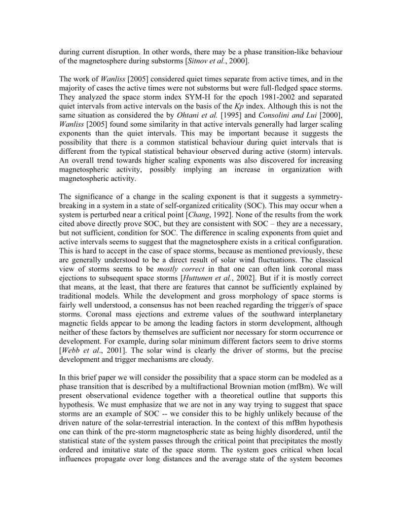
This assumption does not mean that these are the only independent parameters; quite the opposite, there may be a number of other suitable parameters. The space storm situation we are considering is analogous to a system close to a gas/fluid phase transition. Such a system is well characterized by pressure P and temperature T. At this point, the comparison is purely formal, based on analogous behavior. Connecting Kp with P and DST with T, we shall demonstrate that this analogy will be able to explain one of the paradoxical features observed in storm dynamics [Wanliss, 2005, and references therein]. If at sufficiently low Kp (i.e. quiet at high latitudes) one finds that DST can increase to storm-associated values there is clearly not global storm activity because if there were then Kp would reflect that. Figure 4 shows a plot of DST against Kp from 1963 to 2003, but only for negative DST values so that we can observe the Kp values associated with storms. Since DST is calculated exclusively from low- to middle-latitude magnetometer stations, and Kp includes higher latitude stations one finds during active times such as space storms, that Kp is generally large, and DST reaches large negative values. Large Kp is the result of the expansion of the auroral oval during magnetospheric activity, such as space storms and magnetospheric substorms. What Figure 4 demonstrates is that sometimes DST indicates an intense or smaller storm even though Kp ≤ 1. If one were to rely on DST alone one might conclude the occurrence of an intense global space storm, yet with Kp ≤ 1 we have the suggestion of no substorms or high-latitude activity. Substorms, with their associated larger Kp values, are a nearly ubiquitous feature of space storms, hence the name substorms. Yet Figure 4 indicates that large DST can occur without global storm activity. These observations suggest that there is some ambiguity in identification of storm onsets. Let us now utilize our analogy. In a thermodynamic system with a phase transition of the first kind, a situation can happen in which the phase curve on the P-T diagram abruptly ends at a critical point (Figure 5). For higher pressure and temperature, the distinction between the two phases is impossible unless they are in contact with each other [Landau and Lifshitz, 1980]. If we vary P and T along a path in P-T space that does not intersect the phase curve, it is possible to pass from one phase to another without noticing any abrupt change. Now, in a strictly formal sense we can use the same reasoning for Kp and DST parameters. In a formal Kp-DST space, if one keeps Kp low while increasing DST, it is possible to pass into an area corresponding to storm behavior without observing storm onset (phase transition). This could explain why at times DST apparently signals a storm while Kp signals a quiet time. There are also more physical reasons for connecting DST with temperature and Kp with pressure. DST corresponds to dynamics at lower latitudes, thus related to dynamics in the near-Earth plasma sheet, an area with a more significant thermal component of plasma. On the other hand, Kp characterizes the higher latitude region, corresponding to a more tail-like field and cooler plasma, where the magnetic stress (negative pressure) is more important. Thus energy can be released from the hotter region while the change does not cause simultaneous release of energy at high latitudes.

Figure 5. P-T phase diagram. Point Pc, Tc is a critical point. If one follows for instance the path from state 1 to state 2 denoted by the dotted line, it is possible to change phase without ever going through a phase transition. The solid line denotes the phase curve. Transition to a lower energy state, such as during a storm, results in a higher degree of organization (larger scaling exponent) as the excess of energy is dissipated. In terms of the physics, the space storm is certainly an example of a process that results in drastic system collapse and reordering, reminiscent of all the arguments described. However, we must carefully note that treating storms as phase transitions is more or less a formal issue at this point. Space storms are significantly more complex than a water and vapor system, since huge numbers of topological structures exist within magnetosphere. Nevertheless, on the basis of our observations, one can hypothesize the existence of a critical transition between a mostly disordered state and an ordered one, separated by a phase transition which is the onset of the space storm. Although formal, this approach is helpful in explaining some of the observed features of storm dynamics that are difficult to explain in traditional models. 5. Conclusion The self-similarity that exists near the critical point (e.g. Figure 3b) is why local imitation cascades through the scales into global coordination. The difference in scaling exponents from quiet and active intervals suggests that the magnetosphere exists in a critical configuration. Whereas prior to the onset of the space storm the nonlinear scaling exponent was varying only slowly and continuously, reminiscent of a second order type phase transition from one critical state to the next, the onset of the storm resulted in a dramatic change such as might result from a dynamical instability characterized by a first-order-like topological phase transition [Chang et al., 2003]. Transition to a lower

P

T TC

PC

2

1

energy state, such as a storm, thus results in more organization (larger scaling exponent) as the excess of energy is dissipated. Once the excess of energy has been dissipated during the recovery phase it results in less organization, and the corresponding reduction in the scaling exponent to pre-storm values. This has possible operational value since the notion of a critical point has as one of its properties the ability to provide some universal predictions, even in the absence of a detailed model, by using what amounts essentially to generalized symmetry arguments. We will examine this idea in a future paper. Acknowledgements This material is based on work supported by the National Science Foundation under Grants No. ATM-0449403 and DMS-0417690. SYM-H data are provided by the World Data Center for Geomagnetism, Kyoto.

References Abramenko, V. I., V. B. Yurchyshyn, H. Wang, T. J. Spirock, and P. R. Goode (2003),

Signature of an avalanche in solar flares as measured by photospheric magnetic fields, Astrophys. J., 597:1135.

Cannon, M. J., D. B. Percival, D. C. Caccia, G. M. Raymond and J. B. Bassingthwaighte (1997), Evaluating Scaled Windowed Variance Methods for Estimating the Hurst Coefficient of Time Series, Physica A, 241, 606-626.

Chang, T. (1992), Low dimensional behaviour and symmetry breaking of stochastic systems near criticality: can these effects be observed in space and in the laboratory?, IEEE Trans. Plasma Sci., 20, 691.

Chang, T, S. W. Y. Tam, C.-C. Wu, and G. Consolini (2003), Complexity, Forced and/or Self-organized Criticality, and Topological Phase Transitions in Space Plasmas, Space Science Reviews, 107, 425-445.

Consolini, G., and Lui A. T. Y. (2000), Symmetry breaking and nonlinear wave-wave interaction in current disruption: possible evidence for a dynamical phase transition, in Ohtani, S.-I., Fujii, R., Hesse, M., Lysak, R. L. (eds.), Magnetospheric Current Systems, AGU Monograph 118, Washington, D. C., pp. 395.

Chen, Z., P. Ch. Ivanov, K. Hu, and H. E. Stanley (2002), Effect of nonstationarities on detrended fluctuation analysis, Phys. Rev. E, 65, 041107.

Consolini, G., and P. De Michelis (1998), Non-Gaussian distribution function of AE-index fluctuations: Evidence for time intermittency, Geophys. Res. Lett., 25, 4087-4090.

Daglis, I. A., W. Baumjohann, J. Gleiss, S. Orsini, E. T. Sarris, M. Scholer, B. T. Tsurutani, B. Vassiliadis (1999), Recent advances, open questions and future directions in solar terrestrial research, Phys. Chem. Earth (C), 24, 5-28.

Daglis, I. A., J. U. Kozyra, Y. Kamide, D. Vassiliadis, A. S. Sharma, M. W. Liemohn, W. D. Gonzalez, B. T. Tsurutani, and G. Lu (2003), Intense space storms: Critical issues and open disputes, J. Geophys. Res., 108 (A5), 1208, doi:10.1029/2002JA009722.

Freeman, M.P., N. W. Watkins, and DJ Riley (2000), Evidence for a solar wind origin of the power law burst lifetime distribution of the AE indices, Geophys. Res. Lett., 27, 1087-1090.

Gonzalez, W. D., J. A. Joselyn, Y. Kamide, H. W. Kroehl, G. Rostoker, B. T. Tsurutani, and V. N. Vasyliunas (1994), What is a geomagnetic storm?, J. Geophys. Res., 99, 5771.

Hnat, B., S. C. Chapman, G. Rowlands, N. W. Watkins, and M.P. Freeman (2003), Scaling in long-term data sets of geomagnetic indices and solar wind as seen by WIND spacecraft, Geophys. Res. Lett., 30, doi:10.1029/2003GL018209.

Hergarten, S. (2002), Self-organized criticality in earth systems, Springer Academic Press, 49.

Hu, K., P. Ch. Ivanov, Z. Chen, P. Carpena, and H. E. Stanley (2001), Effect of trends on detrended fluctuation analysis, Phys. Rev. E, 64, 011114.

Huttunen, K. E. J., H. E. J. Koskinen, T. I. Pulkkinen, A. Pulkkinen, M. Palmroth, E. G. D. Reeves, and H. J. Singer (2002), April 2000 magnetic storm: Solar wind driver and magnetospheric response, J. Geophys. Res., 107(A12), 1440, doi:10.1029/2001JA009154.

Kaufmann, R.L. (1987), Substorm Currents: Growth Phase and Onset, J. Geophys. Res., 92, 7471-7486.

Kozyra, J. U., M. W. Liemohn, C. R. Clauer, A. J. Ridley, M. F. Thomsen, J. E. Borovsky, J. L. Roeder, V. K. Jordanova, and W. D. Gonzalez (2002), Multistep development and ring current composition changes during the 4-6 June 1991 magnetic storm, J. Geophys. Res., 107(A8), 1224, doi:10.1029/2001JA000023.

Liemohn, M. W., Kozyra, J. U., M. F. Thomsen, J. L. Roeder, G. Lu, J. E. Borovsky, and T. E. Cayton (2001), Dominant role of the asymmetric ring current in producing the storm time Dst*, J. Geophys. Res., 106, 10,883-10,904.

Li, X., D. N. Baker, M. A. Temerin, T. E. Cayton, G. D. Reeves, R. A. Christensen, J. B. Blake, M. D. Looper, R. Nakamura, and S. G. Kanekal (1997), Multi-satellite observations of the outer zone electron variation during the November 3-4, 1993, magnetic storm, J. Geophys. Res., 102, 14,123.

Li, X, M. Temerin, D. N. Baker, G. D. Reeves and D. Larson (2001), Quantitative Prediction of Radiation Belt Electrons at Geostationary Orbit Based on Solar Wind Measurements, J. Geophys. Res., 28, 1887-1890. Lui, A. T. Y. (2002), Multiscale phenomena in the near-Earth magnetosphere, J. Atmos.

Sol.-Terr. Phys., 64, 125. Meredith, N. P., R. M. Thorne, R. B. Horne, D. Summers, B. J. Fraser, and R. R.

Anderson (2003), Statistical analysis of relativistic electron energies for cyclotron resonance with EMIC waves observed on CRRES, J. Geophys. Res., 108(A6), 1250, doi:10.1029/2002JA009700.

Ohtani, S., Higuchi, T., Lui, A.T.Y., and Takahashi, K. (1995), Magnetic fluctuations associated with tail current disruption: Fractal analysis, J. Geophys. Res., 100, 19135.

Peltier, R. and J. Levy Vehel. (1995), Multifractional Brownian motion: Definition and preliminary results, Technical report INRIA 2645.

Peng, C.-K., S. Havlin, H. E. Stanley, A. L. Goldberger (1995), Quantification of Scaling Exponents and Crossover Phenomena in Nonstationary Heartbeat Timeseries, Chaos, 5 (1), 82-87.

Reeves, G. D. (1998), Relativistic electrons and magnetic storms: 1992-1995, Geophys. Res. Lett., 25, 1817-1820.

Richardson, I. G., E. W. Cliver, H. V. Cane (2001), Sources of geomagnetic storms for solar minimum and maximum conditions during 1972-2000, Geophys. Res. Lett., 28, 2569-2572.

Sitnov, M. I., A. S. Sharma, K. Papadopoulos, D. Vassiliadis, J. A. Valdivia, A. J. Klimas, and D. N. Baker (2000), Phase transition-like behaviour of the magnetospheric during substorms, J. Geophys. Res., 105, 12, 955-12, 974.

Takalo, J., J. Timonen, and H. Koskinen (1993), Correlation dimension and affinity of AE data and bicolored noise, Geophys. Res. Lett., 20, 1527-1530.

Taqqu, M. S., V. Teverovsky, and W. Willinger (1996), Estimators for long-range dependence: An empirical study, Fractals, 3, 185.

Vichare, G., S. Alex, and G. S. Lakhina (2005), Some characteristics of intense geomagnetic storms and their energy budget, J. Geophys. Res., 110, A03204, dli:10.1029/2004JA010418.

Wanliss, J.A., J.C. Samson, and E. Friedrich (2000), On the use of photometer data to map dynamics of the magnetotail current sheet during substorm growth phase, J. Geophys. Res., 105, 27673-27684.

Wanliss, J. A. (2004), Nonlinear variability of SYM-H over two solar cycles, Earth Planets Space, 56, e13–e16.

Wanliss, J. A. (2005), Fractal properties of SYM-H during quiet and active times, J. Geophys. Res., 110, A03202, doi:10.1029/2004JA010544.

Wanliss, J. A., and K. Showalter (2005) , The High Resolution Global Storm Index: DST versus SYM-H, in review J. Geophys. Res..

Wanliss, J. A., V. V. Anh, Z.-G. Yu, and S. Watson (2005), Multifractal modelling of magnetic storms via symbolic dynamics analysis, J. Geophys. Res., doi:10.1029/2004JA010996.

Webb, D. F., N. U. Crooker, S. P. Plunkett, and O. C. St. Cyr (2001), The Solar Sources of Geoeffective Structures, in Space Weather, Paul Song, Howard J. Singer, and George L. Siscoe, editors, AGU Geophysical Monograph 125, 123-141.

Wood A. and G. Chan (1994), Simulation of Stationary Gaussian Processes, Journal of Comp. and Graphical Statistics, Vol. 3, 409-432.