spatial clustering of rural poverty and food...
TRANSCRIPT

1
Spatial clustering of rural poverty and food insecurity in
Sri Lanka
Upali Amarasinghe∗∗∗∗ , Madar Samad, Markandu Anputhas
International Water Management Institute, 127, Sunil Mawatha, Pelawatta, Battaramulla,
Colombo, Sri Lanka. Tel: 94-11-2787404. Fax: 94-11-2786854. E-mail addresses:
[email protected]; [email protected]; [email protected]
Abstract
We mapped poverty, with reference to a nutrition-based poverty line, to
analyse its spatial clustering in Sri Lanka. We used the Divisional Secretariat
poverty map, derived by combining the principal component analysis and the
synthetic small area estimation technique, as the data source. Two statistically
significant clusters appear. One cluster indicates that low poverty rural areas
cluster around a few low poverty urban areas, where low agricultural employment
and better access to roads are key characteristics. The other indicates a cluster of
∗ Corresponding author.

2
high poverty rural areas, where agriculture is the dominant economic activity, and
where spatial clustering is associated with factors influencing agricultural
production. Agricultural smallholdings are positively associated with spatial
clustering of poor rural areas. In areas where water availability is low, better
access to irrigation significantly reduces poverty. Finally, we discuss the use of
poverty mapping for effective policy formulation and interventions for alleviating
poverty and food insecurity.
Keywords: Spatial clustering; food poverty line; subdistrict level; water and land resources;
geographical targeting; Sri Lanka
Introduction
Historically, Sri Lanka has placed a high value on basic human needs,
channelling assistance to rural areas to promote food security and employment,
and to assure that the poor have access to primary health care, basic education and
an adequate diet. This policy has resulted in the country achieving significant
advances in some areas of human welfare compared to other low-income
countries. Life expectancy at birth (74 years), infant mortality rate (16 per 1000
live births), adult literacy rate (92%) and the combined primary, secondary and
tertiary school enrolment ratio (66%) at present are comparable to levels in the

3
more developed countries (UNDP, 2003). Yet, about one quarter of the population
remains below the official income poverty line (DCS, 2003).
Over the years, successive governments have introduced various interventions
to alleviate income poverty. But, whether the benefits of these interventions
actually reached those intended is doubted because of shortcomings in identifying
and locating the poor. As in many other countries, Sri Lankan national poverty
assessments are compiled using household and community surveys and
disaggregated into broad categories such as urban, rural and estate sectors and for
a larger geographical unit such as an administrative district. Aggregate poverty
statistics at the resolution of district level are too limiting for identifying spatial
patterns of poverty within and across districts, and for assessing the causes and
effects of spatial variations of poverty in smaller geographical units. There is a
growing demand for poverty information at a finer resolution to enable a narrower
geographic targeting aimed at maximizing the coverage of the poor while
minimizing leakage to the non-poor (Henninger and Snel, 2002).
We use the poverty estimates at Divisional Secretariat (DS) level, a lower
administrative unit than a district, to test whether the poor in Sri Lanka are
spatially clustered, determine how far spatial clustering influences incidence of
poverty and investigate the association of availability and access to water and land
resources and infrastructural facilities with poverty and its spatial clustering
across DS divisions.

4
Subnational poverty maps
Poverty maps depict the spatial variation of indicators of human well-being
across units in geographically disaggregated layers (Henninger, 1998, Hentschel
et al., 2000, Davis, 2002, World Bank, 2004). Sri Lanka is divided into four
administrative layers: 9 provinces, 25 districts, 325 DS divisions and about 14,000
Grama Niladari (GN), or village officer divisions (DCS, 1998). Of the four
administrative layers, the GN division is an ideal unit for subnational poverty
mapping analysis. But we take the DS division as our unit of analysis because of
limitations on the availability of ancillary data for estimating poverty at the GN
level.
The poverty line in this article, an estimate of the cost of a bundle of food
items adequate for receiving the minimum nutritional requirement1 (DCS, 2003),
is essentially a food poverty line. The poverty estimate, the proportion of
households below the food poverty line, represents households that are both poor
and food insecure. A household is poor if it spends more than 50% of its
expenditure on food and its per adult equivalent food expenditure is below the
food poverty line. Thus the poverty estimate here is essentially an indicator of
poverty and food insecurity in Sri Lanka.
The district poverty estimates (Fig. 1B) show no significant variation of
poverty across districts in the North Central, Uva and Sabaragamuwa Provinces
(Fig. 1A). The incidence of poverty in the Anuradhapura and the Polonnaruwa

5
Districts (about 29%) in North Central Province is almost identical so that district-
level poverty maps are too aggregate to find any variation across or within
districts.
The DS divisional poverty estimates (Fig. 1C), derived by combining the
principal component analysis and the synthetic small area estimation technique2
(Amarasinghe et al., in press), vary from 1% to 46%. Even in the provinces, such
as North Central, Uva and Sabaragamuwa, where the variation of poverty across
districts does not seem significant, the variation of poverty across DS divisions is
significant. Moreover, most DS divisions with low incidence of poverty (below 1
standard deviation from the national average) are located in a cluster in the
Colombo and Gampaha Districts, and most DS divisions with high incidence of
poverty (above 1 standard deviation from the national average) are located in a
cluster in four districts: Ratnapura, Badulla, Moneragala and Hambantota. The
distribution of the DS division’s poverty levels is highly skewed (Table 1), with
74% of the DS divisions falling above the national average poverty level.
The DS poverty maps can be useful for spatial targeting of poverty
interventions. The World Bank (2002) reports that while many households in the
upper income strata receive the welfare benefits of the Samurdhi programme3,
designed to help the poor, many in the lower-income strata miss these welfare
benefits. Indeed, the Samurdhi programme has different criteria for identifying the
poor households that are eligible for welfare assistance. But the selection criteria
flaws coupled with regional and local-level political interferences have often
contributed to the Samurdhi programme’s significant leakages to the non-poor.

6
The poverty map can locate DS divisions with highly inefficient resource
allocation (Fig. 2). For example, only 3000 households of the four least poor DS
divisions (category 1 in Fig. 1 and Table 1) are poor but more than 12,000
households receive the highest financial assistance under the Samurdhi welfare
programme. And nine of the poorest DS divisions (category 6 in Fig. 1 and Table
1) have 31,000 poor households but only 19,000 households receive the highest
financial assistance. If resources are distributed proportionately to the poverty
levels of DS divisions, then all poor households can receive welfare benefits at a
level (about 970 LKR4, or about US$10) higher than the highest financial
assistance distributed at present (Amarasinghe et al., 2005). This certainly is
adequate to reduce the food poverty gap or food insecurity of many poor
households and can perhaps reduce the number of food-insecure poor households
in many DS divisions.
Because of the lack of poverty information at geographically disaggregated
unit level, the poverty determinants analyses conducted so far have ignored
poverty and food insecurity for detailed geographic units and the influences of
spatial dependencies of neighbouring units. We investigate the extent of spatial
clustering of poverty across DS divisions and its influence on the incidence of
poverty and the factors associated with spatial clustering of poverty.
Spatial clustering of locations of poverty

7
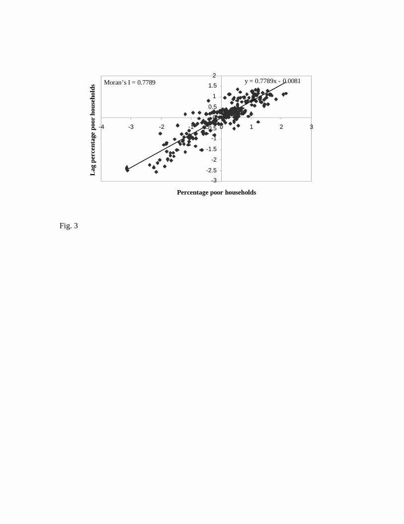
Spatial clustering shows the similarity or dissimilarity of poverty in
neighbouring units and spatial autocorrelation measures the strength of the spatial
clustering (Cliff and Ord, 1973, Getis and Ord, 1992, Anselin, 1995). The global
Moran’s I statistic, the slope of the regression line of the scatterplot of the
standardized percentage of poor households, and spatial lag5 of the percentage of
poor households (Fig. 3) indicate the strength of the spatial similarity of the whole
area. Negative values of x- and y-axes in Fig. 3 indicate below-average values.
The first and the third quadrant points in Fig. 3 suggest positive spatial
autocorrelation and hence similar units. The first quadrant points show high
poverty DS divisions with high poverty neighbours (high-high), while the third
quadrant points show low poverty DS divisions and low poverty neighbours (low-
low). The second and fourth quadrant points suggest negative spatial
autocorrelation and hence dissimilar units. The second quadrant points show low
poverty DS surrounded by high poverty neighbours (low-high) while the fourth
quadrant points show high poverty DS divisions surrounded by low poverty
neighbours (high-low).
Statistically significant global Moran’s I (significant at 0.001 level) confirms
the hypothesis that poor (or non-poor) locations are often found in spatial clusters,
meaning that a poor (or non-poor) location is often surrounded by poor (or non-
poor) neighbours.
Local Moran’s I indicator, estimated using the spatial data analysis package
Geoda 9.0 (Anselin, 2003), identifies the locations with statistically significant

8
spatial autocorrelation. Fig. 4A shows the DS divisions with high and Fig. 4B
with low levels of poverty and surrounded by similar neighbourhoods. Fig 4C
shows DS divisions with low and Fig. 4D with high levels of poverty but
surrounded by dissimilar neighbourhoods.
High poverty DS divisions and high poverty neighbourhoods are mainly rural
(Fig. 4A), and agricultural economic activities are the main source of income of
most households. For example, at least every two in three households have an
agricultural operator in Kurunegala, Anuradhapura, Polonaruwa, Moneragala and
Hambantota Districts. But the similarities are significant in only four districts:
Badulla, Moneragala, Hambantota and Ratnapura (black-shaded units).
Low poverty DS divisions and low poverty neighbourhoods (Fig. 4B) are
mainly found in Puttlam, Gampaha, Colombo, Kalutara, Galle and Kandy
Districts. But the similarities are significant in only Colombo, Gampaha, Kalutara
and Galle Districts (black-shaded units). Only a few of the DS divisions in the
low-low poverty group are urban centres, the rest are mainly rural. Non-
agricultural activities contribute substantially to the household income in rural
units. For example, only 1 in 20 households in Colombo District, 2 in 11
households in Gampaha District, and less than 1 in 3 households in Kalutara,
Galle and Puttalam Districts have an agricultural operator.6 Low agricultural
employment suggests that the economic activities of rural neighbours are closely
associated with the economic activities of urban DS divisions in these districts.
Figs. 4C and 4D show some spatial outliers where these units and their
neighbours have contrasting levels of poverty. The shaded DS divisions in Fig. 4C

9
have low levels of poverty but the neighbouring divisions have high levels.
Moran’s I statistic of these is significant in only the Nuwara Eliya DS division,
which has significant non-agricultural income activities such as tourism but is
surrounded by poor DS divisions with significant agricultural economic activities.
The shaded units in Fig. 4D have high levels of poverty but the neighbouring
units have low levels. But Moran’s I statistic of these units is not significant.
The identification of spatial clusters has many advantages. First, it helps locate
similar and dissimilar neighbourhoods and their influence on incidence of
poverty. Second, it could identify physical, social, economic and institutional
factors that contribute to spatial similarity or dissimilarity. Third, it helps design
effective spatially targeted interventions that can trigger a higher rate of poverty
alleviation within a locality than the intervention designs at national or regional
level.
Spatial association
What are the main determinants of poverty and spatial similarity or
dissimilarity of poverty, especially of the DS divisions in rural areas? More than
three-quarters of the population in Sri Lanka live in rural areas and their main
livelihood is agriculture or agricultural labour. Thus the availability and access to
water and land are crucial factors for the livelihood of poor people. Although the

10
rainfall totals are high in most areas, substantial intra-annual variations are severe
constraints for productive agriculture in many areas. Thus a small quantity of
irrigation is required to supplement water deficits in maha, or the main season,
and irrigation is a must for agriculture in yala, or the second season. So, access to
irrigation through infrastructure is necessary for alleviating poverty in many of
the rural areas. This was substantiated in studies comparing the contribution of
irrigated and rainfed agriculture in reducing poverty (JBIC, 2002).
Successive governments in the past have invested heavily in new irrigation
infrastructures or in rehabilitation of old ones. In fact, irrigation investment was
the major plank of rural development and poverty reduction and of the national
food security strategy. While some districts benefited from these irrigation
investments, others such as Moneragala and Hambantota did not. This is primarily
due to lack of information on geographical distribution of poverty, except where
statistics show that poverty is high in the rural sector. Lack of irrigation facilities
is not the only cause of poverty. There is no information on how poverty is
spatially concentrated and what other factors, such as access to land and
infrastructural facilities, are contributing to spatial concentration of poverty.
Variables used
Availability of and access to water

11
In the absence of data on water availability, seasonal rainfall is taken as a
proxy for this in DS divisions, and the availability of irrigation infrastructure in
major and minor irrigation schemes is taken as a proxy for access to water supply.
A higher level of water availability and access to irrigation infrastructure is
expected to increase agricultural production and, hence, living conditions and to
reduce clustering of poverty. Variables (1 to 4) used were:
1. Average maha season rainfall. The maha season (October to March) is the
main growing season where rainfall needs to be supplemented only with a
little irrigation for crop production. The average maha season rainfall varies
from 730 mm to 1400 mm across DS divisions.
2. Average yala season rainfall. The yala season (April to September) receives
140 mm to 960 mm of rainfall and irrigation is required for crop production in
most areas.
3. The irrigable area under major and 4. minor irrigation schemes as a
percentage of total crop area. The irrigable area under major and minor
irrigation schemes varies from 0% to 79% and 0% to 28% across DS divisions
and indicates the physical area of water availability under irrigation schemes.
The total area equipped with irrigation facilities (both major and minor
irrigation schemes) varies across districts but is substantial in Polonnaruwa
(83%), Anuradhapura (67%) and Hambantota (47%) Districts.
12
Availability of and access to land
The extent of landholding sizes per operator and holding size patterns are taken
as proxies for land availability. The large agricultural landholding areas are
expected to increase income and reduce poverty and, hence, clustering. Variables
(5 to 8) used were:
5. Smallholding7 size per agricultural operator. The average holding size varies
from 0.5 to 1.1 ha.
6. Smallholding area below 0.4 ha varies from 10% to 50%.
7. Smallholding area between 0.4 and 0.8 ha varies from 20% to 36%.
8. Percentage of agricultural operators not owning land varies from 0 to 0.7
(every 7 out of 10 operators).
Employment and infrastructure facilities
The number of agricultural operators shows the extent of population employed
in agriculture. The extent of infrastructure development in DS divisions can be

13
considered as a proxy variable for access to markets and also for access to
employment opportunities, especially for rural people, in the non-agricultural
sectors. Variables (9 to 11) used were:
9. Number of agricultural operators per household indicates the agriculturally
active population per household in each DS division and varies from 0 to 1.21
(almost five agricultural operators in every four households).
10. Average distance to roads8 varies from 0 to 12 km.
11. Average distance to towns is the average of the distance of DS divisions
calculated from towns to a 5- to 8-km buffer zone.
Regression analysis
We assessed the influence of the above factors on the incidence of poverty and
on the spatial clustering of poverty of the DS divisions using ordinary least square
(OLS) regression. The hypotheses here are that spatial clustering of poverty is
significantly associated with the level of poverty of DS divisions and that spatial
clustering of availability and access to water and land and infrastructure (Figs. 5-
7) are significantly associated with spatial clustering of poverty.
Table 2 gives the regression results. Local Moran’s I is included in the OLS2
in Table 2 to assess the influence of spatial similarities or dependence of the

14
neighbouring units on the variations of poverty of the DS division. The increment
of R2 from OLS1 to OLS2 shows the magnitude of the contribution of spatial
dependence in explaining the variation of the level of poverty across the DS
divisions.
The third regression (OLS3 in Table 2) assesses the extent of association of
spatial clustering of explanatory variables on the spatial clustering of the
incidence of poverty. The hypothesis here is that the spatial clustering of access
and availability of land and water are associated with the spatial clustering of the
incidence of poverty. The OLS3 has Local Moran’s I of the percentage of poor
households as the dependent variable and Local Moran’s I of each explanatory
variable in OLS1 as explanatory variable in this case.
OLS on the entire data set
First, the regression analysis is conducted for the entire data. The DS divisions
with lower poverty levels are located in the wet zone9 districts: Colombo,
Gampaha, Kalutara, Galle, Matara, Kandy and Nuwara Eliya. In general, these
units have higher rainfall, smallholdings (mostly homesteads and self-owned),
low agricultural employment, and are close to major urban centres in the districts.
Thus the significant coefficients of OLS1 are not surprising. But the analysis of
the entire data set seems to have masked the association of access to water

15
(availability of irrigation) and poverty, especially in the DS divisions with
agriculture dominating livelihoods.
Although the spatial autocorrelation is significant, inclusion of Local Moran’s I
in the OLS2 regression has not resulted in a significant increase in the explanatory
power of the variation of poverty. Non-significant coefficients of Local Moran’s I
are because the Local Moran’s I is high for both high-high (Fig. 4A) and low-low
(Fig. 4B) poverty clusters, whereas the level of poverty is significantly different
between the two clusters. Therefore, in order to better understand the influence of
the level and spatial clustering of access and availability of water and land on the
level and spatial clustering of poverty, we conduct separate analyses for the two
clusters.
OLS on high-high poverty neighbourhoods
The DS divisions in the high-high poverty cluster are mainly rural and most
livelihoods depend on agriculture. Availability and access to land and water
resources are crucial in reducing poverty. Most of the DS divisions in the high-
high poverty cluster are in the dry zone and have similar rainfall patterns and
water availability. But access to water (explained in terms of major irrigated area)
and land ownership are significantly associated with lower poverty (OLS1).
However, the R2 of OLS1 is small (10%). The OLS2 regression shows that much

16
of the variation of poverty in the high-high poverty cluster is explained by the
local spatial autocorrelation variable. In addition, the higher percentage of minor
irrigated area, where water is stored in small irrigation tanks usually affected by
the intra- and inter-annual variations of rainfall, and lack of land ownership are
positively associated with the higher incidence of poverty. The spatial
autocorrelation variable in OLS2 explains 76% of the variation of poverty
(difference between OLS1 and OLS2 R2s).
In the OLS3 regression, we assess the factors associated with spatial clustering
of poverty. Spatial clustering of two factors, high percentage of irrigated crop
areas and large landholding area per agricultural operator, is associated negatively
with spatial clustering of DS divisions with a high proportion of poor households.
Spatial clustering of two other factors, high percentages of smallholding size
classes (less than 0.4 ha and between 0.4 and 0.8 ha) is associated positively with
spatial clustering of DS divisions with a high proportion of poor households.
The OLS3 regression results indicate the positive influence of the availability
of irrigation water supply and large landholding sizes on the lower spatial
clustering of poor in rural areas. For example, the DS divisions of three districts—
Anuradhapura, Polonnaruwa and Hambantota—have both a high proportion of
irrigated land area and large landholding sizes per operator. But the relatively
larger irrigation areas in Anuradhapura and Polonnaruwa than in Hambantota
make spatial clustering of poor not significant in the former two districts but
significant in the latter district.

17
The DS divisions in Moneragala District also have a large agricultural land
area per operator as in Polonnaruwa District but they have very low irrigation
facilities. Inadequate infrastructural supply providing irrigation is a cause for poor
DS divisions in Moneragala District to be located in spatial clusters.
Badulla and Ratnapura Districts, unlike others, have a low number of
agricultural operators per households. The substantial labour resources in the two
districts engaged in the plantation sector are not counted as agricultural operators.
Of those who are considered agricultural operators, many operate in small
agricultural landholdings. Thus smallholding sizes in these two districts are a
possible cause for the spatial clustering of poor DS divisions.
The analysis on the high-high poverty cluster shows that differential access to
land and water resources is indeed associated with spatial clustering of poor DS
divisions, and is especially true for the significant spatial clustering of DS
divisions in the two districts, Hambantota and Moneragala.
OLS on low-low poverty neighbourhoods
Most of the DS divisions in the low-low poverty cluster (Fig. 4B) are located
in the wet zone. The DS divisions with lower yala season rainfall, larger
landholding sizes per operator, larger proportion of minor irrigated area and long
distance to towns are significantly associated with DS divisions with a high

18
poverty level. The relatively poorer DS divisions in the low-low poverty group
are located away from the main urban centres and the landholdings per household
are large, with a substantial agricultural component supporting the livelihoods of
the people. Although major irrigation is not prominent in the low-low poverty
group, minor irrigation is prominent and is significantly associated with units with
higher poverty.
The inclusion of the spatial autocorrelation variable in the OLS2 regression
shows a slight increase in R2 (about 18%). However, all statistically significant
coefficients in OLS1 except the minor irrigated area were not significant in OLS2.
Nonsignificance of the OLS2 coefficients could be because many of the
explanatory variables in the low-low poverty group are clustered in areas where
low poverty clustering is significant. Here also we conducted a regression analysis
(OLS3) to assess the association of spatial clustering of the explanatory variables
with the spatial clustering of poverty.
The proportion of spatial clusterings of minor irrigated area, number of
agricultural operators per household and average distance to roads are positively
associated with spatial clustering of low poverty DS divisions. And spatial
clustering of the proportion of smallholding sizes (less than 0.4 ha) is negatively
associated.
While the number of agricultural operators, proportion of irrigated area and
average distance to roads are low and similar, the proportion of smallholding sizes
below 0.4 ha is high and similar in the DS divisions and their neighbourhood.

19
These indicate that non-agricultural activities are the major sources of income-
generating activities of the DS divisions in the low-low poverty areas.
The OLS2 regression analysis of the two poverty clusters showing spatial
similarities explains substantial variation of the poverty of DS divisions. The
OLS3 analysis used OLS regression in assessing the association of spatial
clustering of explanatory variables and poverty. However, the statistically
significant global Moran’s Is of errors of OLS3 regression indicate that better
spatial regression models are required to determine the exact magnitude of the
contribution of spatial clustering of explanatory variables on spatial clustering of
poverty. Identification of spatial similarities of poverty and those of contributing
factors are useful for designing spatially targeted interventions for alleviating
poverty. Such interventions can target several factors that are similar in different
spatial clusters.
Conclusions
We assess the spatial patterns of poverty in Sri Lanka at the subdistrict or
administrative DS level. Poverty maps for the DS divisions depict the proportion
of poor households below the official poverty line.
The poverty map shows significant spatial variation of poverty across DS
divisions. The DS division poverty maps can be used for geographical targeting of

20
poverty alleviation interventions. In the Samurdhi poverty alleviation programme,
poverty maps can be used to distribute financial assistance equitably between the
DS divisions. If the allocated resources are then distributed properly, all poor
households can receive substantially higher financial assistance than at present.
This could lead to a significant drop in the food poverty gap and possibly reduce
the food insecurity of many poor households.
The poverty maps also show significant spatial clustering of poor and non-poor
areas. The clusters of DS divisions with a high percentage of poor households are
found in four rural districts where agriculture is the main source of livelihood of
the majority of households. The clustering of DS divisions of low poverty around
major urban centres suggests that, in predominantly agricultural areas, poor
people have only limited economic opportunities to escape poverty.
The analysis also shows spatial autocorrelation, which measures the strength of
spatial clustering, and explains substantial variation of the incidence of poverty
across DS divisions. In rural areas where water is scarce, the spatial clustering of
major and minor irrigated areas and large agricultural holdings are associated with
less spatial clustering of poor households. The clustering of areas with a high
proportion of smallholding sizes (below 0.4 ha) is positively associated with the
clustering of poor DS divisions. This shows that access to irrigation infrastructure
is a major factor in reducing poverty. But, where the agricultural smallholdings
are concentrated, the incidence of poverty tends to be high. Massive investments
in new or rehabilitated irrigation schemes alone may not be an effective
intervention in some poverty-stricken areas.

21
Although the proportion of irrigation land per DS division and the average
landholding sizes are crude proxies for the availability and access to water and
land resources at DS divisional level and may not permit one to derive statistically
valid estimates, the analysis shows that availability of and access to water and
land resources is a major factor of spatial concentration of poverty in rural areas.
The analysis provides an overview of the spatial variations in poverty at a finer
resolution than current national statistics provide at a coarse resolution for an
administrative district. A major constraint in the present analysis is the
unavailability of reliable information, especially for accurately measuring the
access to resources, markets and services. Nonetheless, our analysis provides a
starting point for the development of poverty maps and spatial and statistical
analyses to identify where the poor live and to understand the specifics of why
they are poor.
References
Amararasinghe, U., Samad, M., Anputhas, M., 2005. Locating the poor: spatially disaggregated
poverty maps for Sri Lanka. International Water Management Institute, Colombo, Sri Lanka.
In press.
Anselin, L. 1995. Local Indicators for Spatial Association-LISA. Geographical Analysis 27, 93-
115.
Anselin, L. 2003. GeoDa TM 0.9 users’ guide. Available at: http://sal.agecon.uiuc.edu and at
http://www.csiss.org

22
Cliff, A., Ord, J. K., 1973. Spatial autocorrelation. Pion, London.
Davis, B., 2002. Choosing a method for poverty mapping. Food and Agriculture Organization of
the United Nations, Rome.
DCS (Department of Census and Statistics), 1998. Grama Niladhari divisions of Sri Lanka. DCS,
Colombo, Sri Lanka.
DCS (Department of Census and Statistics), 2003. Poverty indicators, household income and
expenditure survey 2002. DCS, Ministry of Interior, Colombo, Sri Lanka. Available at:
www.census.lk
Getis, A., Ord, J. K., 1992. The analysis of spatial association by the use of distance statistics.
Geographical Analysis 24, 189-206.
Ghosh, M., Rao J. N. K., 1994. Small area estimation: an appraisal. Statistical Science 9(1), 55-93.
Henninger, N., 1998. Mapping and geographic analysis of poverty and human welfare: review and
assessment. Report prepared for the United Nations Environment Programme-Consultative
Group on International Agricultural Research (UNEP-CGIAR) Consortium for Spatial
Information. World Resources Institute, Washington DC.
Henninger, N., Snel, M., 2002. Where are the poor? Experiences with the development and use of
poverty maps. World Resources Institute, Washington DC and United Nations Environment
Programme/Global Resources Information Database (UNEP-GRID) Arendal, Norway.
Hentschel, J., Lanjouw, J., Lanjouw, P., Poggi, J., 2000. Combining census and survey data to
trace the spatial dimensions of poverty: a case of Ecuador. World Bank Economic Review
14(1), 147-165.
JBIC (Japan Bank for International Cooperation), 2002. Impact assessment of irrigation
infrastructure development on poverty alleviation: a case study of Sri Lanka. JBIC Research
Report no. 19, Tokyo, Japan. Available at: http://www.jbic.go.jp/english/research/report
/paper/index.php
UNDP (United Nations Development Programme), 2003. World human development report.
UNDP, New York.

23
Vidyaratne, S., Tilakaratne, K. G., 2003. Sectoral and provincial poverty lines for Sri Lanka.
Department of Census and Statistics, Colombo, Sri Lanka.
World Bank, 2002. Sri Lanka poverty assessment. World Bank, Washington DC.
World Bank. 2004. About poverty maps. Available at:
http://www.worldbank.org/poverty/aboutpn.htm.
1 The minimum daily calorie requirement estimate for an adult is 2030 Kcal (Vidyaratne and
Tilakaratne, 2003).
2 The poverty level of a DS division is estimated using the “synthetic area” small area
estimation method (Ghosh and Rao, 1994). The number of poor households of a DS division is
estimated using Eq. 1:
i
jij
ijij Y
II
Y ˆˆ∑
= (1)
where iY is the survey estimate of the number of poor households of the ith district and ijI is the
value of the index generated using auxiliary variables of the jth DS division in the ith district. The
index ijI is proportional to a linear combination (1.694 Z1 + 1.822 Z2) of the first two principal
components of 30 variables ranging from household demography, assets, agricultural employment,
agricultural productivity, agricultural income and proximity to infrastructural facilities. At the
district level, poverty = district dummies + 1.694 Z1 + 1.822 Z2, R2= 0.68 (for details, see
Amarasinghe et al., in press).
3 The Samurdhi programme has three main components: (1) welfare or consumption grants, (2)
savings and credits and (3) rural infrastructural development. The welfare component provides
financial support and serves short-term goals and claims 80% of the total Samurdhi budget. The
other two components have long-term objectives in reducing poverty.
4 LKR = Sri Lankan rupee. US$1 = 95 LKR in 2002.

24
5 The spatial lag variable is calculated using the eight nearest neighbours of DS divisions.
6 Agricultural operator is defined as a person responsible for operating agricultural land or
livestock or both, conducts activities alone or with assistance from others or only directs day-to-
day operations (DCS, 2003).
7 Smallholdings are defined as agricultural areas below 8 ha.
8 The distance to roads and towns is the average of the Euclidean distances from the centre of
the source cell to the centre of the surrounding cells. We calculated the Euclidean distance grid
using ArcInfo GRID.
9 Rainfall patterns divide Sri Lanka into three climatic zones: wet, intermediate and dry. The
wet zone receives more than 2500 mm of annual rainfall, the intermediate zone between 1750 and
2500 mm, and the dry zone less than 1750 mm of annual rainfall.

Figure Legends Fig. 1. Spatial variation of percentage of poor households across (A) provinces, (B)
districts and (C) Divisional Secretariat divisions.
Fig. 2. Difference between the percentage of the Samurdhi programme’s households
with the highest financial assistance and percentage of households below the poverty line.
Fig. 3. Scatterplot of percentage poor households versus lag percentage poor households.
Fig. 4. Divisional Secretariat (DS) divisions with statistically significant spatial
autocorrelation of percentage of poor households of (A) high poverty unit and high
poverty neighbourhood, (B) low poverty unit and low poverty neighbourhood, (C) low
poverty unit and high poverty neighbourhood, and (D) high poverty unit and low poverty
neighbourhood. Note that the spatial autocorrelation is estimated for all DS divisions
except for those in the Northern and Eastern provinces.
Fig. 5. Spatial similarity or dissimilarity of (A) percentage of major irrigated area, and
(B) percentage of minor irrigated area within the (I) high-high and (II) low-low poverty
clusters.
Fig. 6. Spatial similarity or dissimilarity of (A) smallholding size per agricultural
operator, and (B) smallholding size below 0.4 ha within the (I) high-high and (II) low-
low poverty clusters.

Fig. 7. Spatial similarity or dissimilarity of (A) number of agricultural operators per
household, and (B) average distance to roads within the (I) high-high and (II) low-low
poverty clusters.

Fig. 1

Fig. 2
-3-2.5
-2
-1.5
-1-0.5
0
0.5
1
1.52
-4 -3 -2 -1 0 1 2 3
y = 0.7789x - 0.0081
Percentage poor households
Lag
per
cent
age
poor
hou
seho
lds Moran’s I = 0.7789
Fig. 3

Fig. 4

Fig. 5

Fig. 6

Fig. 7

Table 1 Summary statistics: distribution of Divisional Secretariat (DS) divisions, percentages of poor households and population over different poverty groups
Households Population Poverty group (% of poor
households)a
DS divisionsb
(no.) Total (1000s)
% below poverty line
Total (1000s)
% below poverty line
1 1.0 - 6.9 4 236 1.1 968 1.3 2 6.9 – 15.3 19 686 11.7 3035 13.9 3 15.3 - 23.7 45 820 19.7 3507 24.0 4 23.7 - 32.1 105 1310 28.6 5208 33.9 5 32.1 - 40.5 67 761 35.5 3242 40.9 6 40.5 - 46.0 9 72 42.6 315 49.4
Total (Ave.) 249 3885 (23.7) 16,275 (27.8)
Source: Authors’ estimates. a The incidences of poverty of groups 3 and 4 are 1 standard deviation (SD) below and above the national average, of groups 2 and 5 are between 1 and 2 SD below and above the national average and of groups 1 and 6 are beyond 2 SD below and above the national average. b Poverty estimates are available for 16 districts outside the north and the east. These districts have 249 DS divisions. The average poverty of DS divisions is 23.7% and the SD is 8.4%.

Table 2 Coefficients of regressions assessing determinants of poverty and poverty clustering and standard errors, with standard errors in parentheses
Explanatory variables Divisional Secretariat (DS) divisions in the analysis All DS divisions
(n = 249) DS divisions with high-high poverty
neighbourhoods (n = 138)
DS divisions with low-low poverty neighbourhoods
(n = 84) OLS1a OLS2a OLS1a OLS2a OLS3b OLS1a OLS2a OLS3b
1. Average maha season rainfall (mm) 0.14 (0.10) 0.12 (0.09) -0.09 (0.08) 0.04 (0.03) 0.06 (0.07) 0.91 (0.22)* 0.02 (0.17) 0.29 (0.22) 2. Average yala season rainfall (mm) -0.41 (0.11)* -0.32 (0.11)* -0.01 (0.09) 0.03 (0.04) 0.04 (0.09) -1.32 (0.21)* -0.09 (0.15) -0.34 (0.29) 3. Major irrigation area (% total crop area) 0.01 (0.05) 0.01 (0.6) -0.09 (0.05)* -0.02 (0.02) -0.11 (0.03)* 0.34 (0.30) 0.03 (0.18) 0.29 (0.96) 4. Minor irrigation area (% total crop area) 0.003 (0.05) 0.01 (0.5) -0.02 (0.04) 0.05 (0.02)* -0.08 (0.03)* 0.02 (0.10)* 0.16 (0.07)* 0.71 (0.27)*5. Smallholding size per agric. operator (ha) 0.15 (0.07) 0.05 (0.8) -0.18 (0.11) 0.02 (0.04) -0.20 (0.11)* 0.30 (0.10)* -0.11 (0.07) 0.37 (0.21) 6. Smallholding area below 0.4 ha (%) 0.05 (0.07) -0.05 (0.07) -0.31 (0.14)* -0.06 (0.05) 0.42 (0.16)* 0.07 (0.06) -0.03 (0.04) -0.72 (0.18)*7. Smallholding area between 0.4 and 0.8 ha (%) 0.38 (0.05)* 0.31 (0.05)* 0.02 (0.07) 0.01 (0.02) 0.54 (0.11)* 0.11 (0.09) 0.00 (0.05) -0.05 (0.17) 8. Agricultural operators not owning land (%) 0.16 (0.05)* 0.16 (0.05)* 0.08 (0.4) * 0.04 (0.02)* -0.01 (0.07) 0.13 (0.17) -0.07 (0.10) 0.26 (0.72) 9. No. of agricultural operators per household 0.18 (0.06)* 0.16 (0.07)* -0.04 (0.05) -0.02 (0.02) 0.03 (0.04) 0.01 (0.14) 0.05 (0.09) 1.83 (0.31)*10. Average distance to roads (km) -0.03 (0.07) 0.10 (0.05) 0.04 (0.05) 0.01 (0.02) -0.02 (0.07) -0.12 (0.25) -0.03 (0.15) 2.53 (0.75)*11. Average distance to towns (km) 0.12 (0.06)* 0.10 (0.05)* 0.01 (0.05) -0.02 (0.02) -0.03 (0.04) 0.22 (0.07)* 0.06 (0.05) -0.01 (0.11)
Local Moran’s Ic - -0.13 (0.05)* - 0.75 (0.02)*
- - -0.37 (0.03)* -
Adjusted R2 0.52 0.53 0.10 0.86 0.16 0.72 0.90 0.87 Global Moran’s I of errors 0.55 0.54 0.46 0.02 0.43 0.30 0.14 0.38
aOLS1 and OLS2 incidence of poverty as dependent variable, % poor households. bOLS3 local spatial autocorrelation of incidence of poverty as dependent variable, local Moran’s I. cLocal spatial autocorrelations of % poor households. * Significant at least at p = 0.05 level.