‘spatial epidemiology of lung cancer mortality

‘Spatial Epidemiology of Lung Cancer Mortality: Geographical Heterogeneity and Risk-Factors Assessment’

Supervisors:

Dr. Richard J.Q. McNally

Prof. Stephen P. Rushton

Dr. Mark S. Pearce

PhD student name: Basilio Gómez-Pozo

Student number: 069 118 278

Institute of Health and Society Sir James Spence Institute (Level 4)

Royal Victoria Infirmary

Queen Victoria Road, Newcastle NE1 4LP

Email: [email protected]

[email protected]

[email protected]

Date of first registration: 13/12/2006

Date of report submission: 12/12/2011

mailto:[email protected]�



i

Abstract

Cancer is the leading cause of mortality in Andalucía (southern Spain) for both men

and women, and lung cancer is the main cause of cancer mortality for men. Radon-gas

exposure is the second most important cause of lung-cancer after tobacco-smoking,

which also causes larynx cancer, and Chronic Obstructive Pulmonary Disease

(COPD). Radon-gas is a radioactive decay element which originates from radium.

Consequently, presence in the soil varies according to lithology (rock composition)

which is a surrogate measure for potential radon-gas exposure. Lithology can explain

some lung-cancer deaths, but not deaths due to either larynx cancer or COPD.

A small-area analysis was implemented for the period 1986-1995. Fully-Bayesian

regression analysis was used to assess the association between lithology and the spatial

distribution of lung-cancer deaths (25,006 cases). Area-level deprivation, a surrogate

measure for tobacco-smoking, was accounted for. The number of deaths due to larynx

cancer (3,653 cases) and COPD (5,143 cases) were also modelled for comparison

purposes. Computation was accomplished via Markov Chain Monte Carlo methods,

using WinBUGS software.

The spatial distribution of lung-cancer deaths (but neither larynx cancer, nor COPD)

was positively associated with lithology, which is consistent with current

epidemiological knowledge. These results remained after adjusting for area-level

deprivation. The model used allows for separate estimation of risk due to both

lithology (RR = 1.02; 95% Credible Interval (CI) = 1.015 – 1.031) and deprivation

(RR = 1.04; 95% CI = 1.033 – 1.048). This lithology score overcomes the difficulties

in obtaining actual radon-gas measurements, and can be further improved. The results

go some way to explaining the regional variability in lung cancer mortality in

Southern Spain.

ii

Dedication

In memory of José María Baena Arjona, my father in law.

iii

Acknowledgmentsi

Doing a research thesis is not only a professional endeavour and a personal challenge,

but also a great human experience. I am deeply indebted to the many people that have

made contributions, directly or indirectly, to ease the way for this piece of research to

be accomplished.

Dr Richard J.Q. McNally guided me through the whole process from the very

beginning (when I was still in Spain, and this research thesis was only a project) until

the writing up and submission stages. Our weekly meetings helped me build

progressively the scaffolding leading to this study. He also gave me the opportunity to

work for the Institute of Health and Society (IHS), where I had the privilege of

working together with, and learning from, many colleagues.

Prof Stephen P. Rushton kept visiting us at the Sir James Spence Institute on a weekly

basis, for about two years. During that period, he provoked on me a serious

conversion: since then, I cannot help thinking of the letter R. Later on, it was two of us

that used to pay him back weekly visits; I think it was then, when he became overtly

Bayesian.

Dr Mark S. Pearce was always willing to read any progress report (even on trains, or

planes) and tried his best to keep me on track. His epidemiological perspective and

critical appraisal were always very useful to me. I wish I could have managed my time

more efficiently, so that I had had the opportunity to read all the books he was willing

to lend me.

I am also grateful to my assessors, Prof Tanja Pless-Mulloli and Dr Roy Sanderson.

They always read my progress reports with interest and made useful suggestions,

which motivated me to keep working.

Dr Jane Salotti and Dr Peter W. James carefully proofread various drafts of this thesis.

I hope I have been able to put into practice most of their advice, as I really appreciate

their time and effort.

To all of them, and many others who cannot be individually acknowledged in such a

short space, my most sincere gratitude.

iv

i This PhD thesis has been partially funded through a fellowship granted by the Spanish body Instituto de Salud Carlos III (ref BAE06/90003). The mortality data were kindly provided by the Andalusian Health Office, department of Information and Evaluation (Dr J. García León), through the Andalusian Mortality Registry (Dr M. Ruiz Ramos).

v

Table of contents

Abbreviations and glossary ......................................................................................viii

List of tables ........................................................................................................... xvii

List of figures .......................................................................................................... xix

Chapter 1. Introduction ............................................................................................... 1

1.1 Background ....................................................................................................... 1

1.2 Rationale ........................................................................................................... 5

1.3 Main Hypotheses ............................................................................................. 10

1.4 Secondary hypotheses ..................................................................................... 10

1.5 General Aim .................................................................................................... 10

1.6 Specific objectives .......................................................................................... 10

1.7 Introduction summary ..................................................................................... 11

Chapter 2. Literature review ...................................................................................... 12

2.1 Aims and strategy ............................................................................................ 12

2.2 Overview ........................................................................................................ 12

2.3 Spatial heterogeneity of mortality in Andalucía ............................................... 13

2.4 Main causes of mortality ................................................................................. 19

2.4.1 Aetiology and epidemiology of lung cancer .............................................. 26

2.4.2 Aetiology and epidemiology of Chronic Obstructive Pulmonary Disease

(COPD) ............................................................................................................. 32

2.4.3 Aetiology and epidemiology of larynx cancer ........................................... 37

2.5 Socio-economic status and mortality due to cancer .......................................... 40

vi

2.6 Radon-gas exposure ........................................................................................ 45

2.6.1 Joint effect of radon-gas exposure and tobacco smoking ........................... 51

2.6.2 Literature review summary ....................................................................... 53

Chapter 3. Data collection and handling .................................................................... 55

3.1 Overview ........................................................................................................ 55

3.2 Administrative Boundaries and lithological data .............................................. 55

3.3 Mortality data .................................................................................................. 58

3.4 Population and socio-economic data ................................................................ 61

Chapter 4. Methods ................................................................................................... 65

4.1 Overview ........................................................................................................ 65

4.2 Health outcomes estimates .............................................................................. 66

4.2.1 Estimates of the expected number of cases ................................................ 66

4.2.2 Modelling of Standardised Mortality Ratios .............................................. 70

4.3 Software description and analysis implementation ........................................... 75

4.4 Ecological analysis .......................................................................................... 78

4.4.1 Socio-economic Status .............................................................................. 78

4.4.2 Potential radon-gas exposure .................................................................... 78

4.5 Disease Mapping ............................................................................................. 79

Chapter 5. Results ..................................................................................................... 82

5.1 Overview ........................................................................................................ 82

5.2 Structural Equation Modelling ......................................................................... 83

vii

5.2.1 Measurement model ................................................................................. 83

5.2.2 Structural model ....................................................................................... 87

5.2.3 Summary of the Structural Equation Model .............................................. 92

5.3 Lung-cancer mortality modelling ..................................................................... 92

5.3.1 Besag-York-Mollié model: males ............................................................. 92

5.3.2 Besag-York-Mollié model: females ........................................................ 107

5.3.3 Mapping of lung-cancer mortality modelling: males ............................... 114

5.3.4 Mapping of lung-cancer mortality modelling: females ............................ 132

5.4 Summary of lung-cancer mortality modelling ................................................ 136

Chapter 6. Discussion ............................................................................................. 137

6.1 Findings ........................................................................................................ 137

6.2 Strengths and limitations ............................................................................... 143

6.2.1 Bayesian analysis and modelling ............................................................ 143

Chapter 7. Conclusions ........................................................................................... 151

7.1 Summary ....................................................................................................... 151

7.2 Contribution .................................................................................................. 152

7.3 Future research .............................................................................................. 153

Chapter 8. References ............................................................................................. 155

viii

Abbreviations and glossary

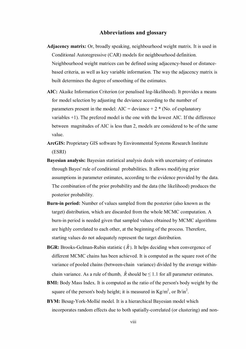
Adjacency matrix: Or, broadly speaking, neighbourhood weight matrix. It is used in

Conditional Autoregressive (CAR) models for neighbourhood definition.

Neighbourhood weight matrices can be defined using adjacency-based or distance-

based criteria, as well as key variable information. The way the adjacency matrix is

built determines the degree of smoothing of the estimates.

AIC: Akaike Information Criterion (or penalised log-likelihood). It provides a means

for model selection by adjusting the deviance according to the number of

parameters present in the model: AIC = deviance + 2 * (No. of explanatory

variables +1). The prefered model is the one with the lowest AIC. If the difference

between magnitudes of AIC is less than 2, models are considered to be of the same

value.

ArcGIS: Proprietary GIS software by Environmental Systems Research Institute

(ESRI)

Bayesian analysis: Bayesian statistical analysis deals with uncertainty of estimates

through Bayes' rule of conditional probabilities. It allows modifying prior

assumptions in parameter estimates, according to the evidence provided by the data.

The combination of the prior probability and the data (the likelihood) produces the

posterior probability.

Burn-in period: Number of values sampled from the posterior (also known as the

target) distribution, which are discarded from the whole MCMC computation. A

burn-in period is needed given that sampled values obtained by MCMC algorithms

are highly correlated to each other, at the beginning of the process. Therefore,

starting values do not adequately represent the target distribution.

BGR: Brooks-Gelman-Rubin statistic ( R̂ ). It helps deciding when convergence of

different MCMC chains has been achieved. It is computed as the square root of the

variance of pooled chains (between-chain variance) divided by the average within-

chain variance. As a rule of thumb, R̂ should be ≤ 1.1 for all parameter estimates.

BMI: Body Mass Index. It is computed as the ratio of the person's body weight by the

square of the person's body height; it is measured in Kg/m2, or lb/in2 .

BYM: Besag-York-Mollié model. It is a hierarchical Bayesian model which

incorporates random effects due to both spatially-correlated (or clustering) and non-

ix

spatial heterogeneity. The inclusion of these effects are responsible for the local and

global smoothing effects, respectively, of RRs estimates.

CAR model: Conditional Autoregressive model. It is used in spatial epidemiology for

local smoothing of RRs estimates, by means of adjacency matrices, or broadly

speaking, neighbourhood weight matrices.

Carstairs-Morris index: Area-level socio-economic index, which is indicative of

material deprivation. The census variables used to build this index are:

overcrowding, male unemployment, low social class, and lack of car ownership.

CH: Spatially-correlated heterogeneity, or general clustering. It is one of the two

components of the residual variance within the BYM model.

CI: Credible Interval. The CI summarises the range of values of the posterior

distribution that encompasses a specified area (e.g. 95% CI); that is to say, the

parameter of interest is itself a variable. Conversely, a confidence interval (its

frequentist counterpart) is the range of values containing the true parameter (in this

case an unknown constant) with certain probability, if a sample was repeatedly

drawn.

CO: Carbon Monoxide. It is a colourless, odourless, and tasteless gas which is a toxic

ambient-air pollutant produced by incomplete combustion of compounds that

contain carbon, such as biomass fuel, or vehicles exhaust. Tobacco smoking is also

a CO source.

CO2: Carbon dioxide. CO2 is a byproduct of normal human metabolism which is

expelled with the air exhaled through the lungs. CO2

Compositional variables: Individual-level characteristics.

is also produced by burning

fossil fuel, as well as from decomposing vegetation, or chemical reactions in the

soil.

Contextual variables: Area-level (geographical) characteristics.

COPD: Chronic Obstructive Pulmonary Disease. COPD is a health condition that

causes permanent damage of the air flow and eventually leads to disability and

death. COPD is known to be mainly due to tobacco smoking.

CR: Confirmation rate. CR, or Positive Predictive Value (PPV), is the conditional

probability of cases being classified as cancer by the gold standard (clinical records

and/or pathology), given that they were classified as cancer by death certificates.

x

CRF: Chronic Respiratory Failure. CRF is characterised by high levels of CO2

CVD: Cardiovascular Diseases. The most important causes of CVD mortality are:

Ischaemic Heart Disease (or heart attack) , Cerebrovascular Disease (or stroke), and

Hypertensive Heart Disease (or high blood pressure).

in the

blood (hypercapnia), low levels of oxygen (hypoxemia), or both. COPD is

frequently associated with CRF.

DIC: Deviance Information Criterion. DIC is the the Bayesian counterpart of the AIC

when applied to multilevel models. The DIC is computed from the mean posterior

deviance and the effective number of parameters (pD). DIC = mean deviance * pD.

DNA: deoxyribonucleic acid. DNA is responsible for the transmission of the genetic

information and, hence, the hereditary characteristics of individuals.

DNA-adducts: Linking of DNA with chemical susbstances (e.g. TSNs). Although

DNA-adducts are supposed to be initiated by the human body as a detoxifying

mechanism, this process actually triggers carcinogenesis.

DR: Detection rate. DR (or sensitivity) is the conditional probability of cases being

classified as cancer by death certificates, given that they were classified as cancer

by the gold standard (clinical records and/or pathology).

EB: Empirical Bayes. EB estimation is a type of Bayesian analysis where the prior

probabilities are obtained from the data under scrutiny. Conversely, in Fully

Bayesian analysis (as in the present research study), the prior probabilities are

obtained from information other than the data under analysis (in this case, data from

a previous time period).

Ecological fallacy: Systematic bias that happens when group-level characteristics are

attributed to the individuals. This is why findings from ecological studies need

confirmation at the individual level.

Ecological study: Epidemiological study-design that gathers information at the group-

level (instead of the individual-level), for both the exposure and event of interest.

EPA: US Environmental Protection Agency.

Epi Map: Free software for statistical analysis and mapping, by the US Centers for

Disease Control and prevention (CDC).

EPIC: European Prospective Investigation into Cancer and nutrition.

ETS: Environmental Tobacco Smoke. Also known as secondhand, passive, or

involuntary tobacco smoking.

FB: Fully Bayesian analysis (see EB).

xi

FEV1: Forced Expiratory Volume in 1 second. FEV1 is obtained by spirometry (test

of respiratory function) and is correlated to the magnitude of airway obstruction and

quality of life, in patients with COPD.

GeoBUGS: WinBUGS add-on software for mapping.

GeoDa: Free GIS software by Luc Anselin.

GIS: Geographic Information Systems.

GRASS: Geographic Resources Analysis Support System. Free, open source, GIS

software.

GSTMG1: enzyme glutathione S-transferase mu gene. Although DNA-adducts are

responsible for triggering carcinogenesis, lack of DNA adducts formation due to the

inherited absence of GSTMG1 can also promote tumorigenesis.

Hyperparameters: Parameters of prior distributions. Contrary to the frequentist

approach (where parameters are considered to be unknown constants), in Bayesian

statistics parameters (and hyperparameters) are considered to be variables with their

own probability distribution.

Hierarchical regression model: Also known as random-effects model, multilevel

model, or mixed model. Hierarchical regression allows for the computation of

estimates with lower MSE than non-hierarchical modelling; this is achieved as

parameter estimates come from data grouped within hierarchies (e.g. deaths within

municipalities). Parameter estimates are pooled down in relation to their variance

(see Smoothing). The BYM model is a Bayesian hierarchical model.

HRQoL: Health-Related Quality of Life.

IARC: International Agency for Research on Cancer.

ICD: International Classification of Diseases.

Iteration: Every value sampled from the posterior distribution by means of MCMC

algorithms, such as Metropolis-Hastings and Gibbs sampling.

INE: Spanish National Statistics Institute

IQR: Interquartile range. The IQR is a measure of statistical dispersion, which is

computed as the difference between the 3rd and the 1st

Kriging: Method of interpolation of unknown values, based on sample points.

quartiles.

LET: Linear Energy Transmission.

Lithology: Rock composition. According to lithology, the main types of rocks are:

sedimentary, plutonic, volcanic and metamorphic.

MAGNA: Spanish National Geological Map.

xii

MAPE: Mean Absolute Predictive Error. As DIC, MAPE can be used as a measure of

goodness of fit of the model. Together with MSPE, MAPE is a loss function which

compares observed and predicted values and it is computed according to the

formula: MAPEj = ∑i │Y i - Yijpred │∕ m, where Y i and Yij

pred denotes the ith

observed and predicted data, respectively, under each model (j subscript), while m

represents the number of observations. An alternative measure is MSPE (Mean

Square Predictive Error); MSPEj = ∑i (Yi - Yijpred )2

MC error: Monte Carlo error. MC error measures the variability of the estimates

obtained by MCMC simulation. The MC error should be kept lower than 5% of the

posterior standard deviation of the correponding parameter estimate. In this case,

convergence is considered to have been reached. The more values are simulated, the

lower the MC error will be.

∕ m. Models with lowest values

of MAPE and MSPE are preferred.

MCMC: Markov Chain Monte Carlo methods. MCMC are a set of algorithms devised

for sampling of random values from a target distribution. Simulation, that is,

generation of pseudo-random numbers, is the basis for Monte Carlo methods. When

many different values are simulated, a chain is said to be obtained. If any future

value does not depend on previous estimates, a Markov process is being used. Both

Metropolis-Hastings and Gibbs sampling algorithms are MCMC methods.

Meta-analysis: Quantitative statistical method for synthesising results of research

studies.

MLE: Maximum Likelihood Estimate. The one with highest probability under the

probability distribution assumed for the sampled data.

MSE: Mean Square Error. A frequentist criterion for reliability of estimates, that

accounts for both bias and variance simultaneously. Bayesian computation can

produce estimates with lower MSE than their frequentists counterparts; this is due to

higher precision of the estimates obtained by MCMC methods.

MSPE: Mean Square Predictive Error (see MAPE).

NCO: Spanish National Classification of Occupations.

NHL: non-Hodgkin's lymphoma. NHL is a large group of malignant lymphomas

originated from either B or T lymphocytes.

NHST: Null Hypothesis Significance Testing. Frequentist statistical method used to

measure the evidence against (null hypothesis) the research (alternative) hypothesis.

NHST make use of p values and confidence intervals. Decisions made by means of

xiii

NHST are subject to the so called type I (where the null hypothesis is wrongly

rejected) and type II (if the null hypothesis is erroneously not rejected) errors.

NO2: Nitrogen Dioxide. NO2

NPV: Negative Predictive Value. NPV is the conditional probability of a person being

healthy given that the diagnostic test was negative.

is a toxic gas from sources such as automobile engines

and tobacco smoking.

Overdispersion: It is present when the variance of a random variable is larger than the

mean. Under these circumstances the Poisson assumption can no longer be upheld.

Overdispersion can be due to spatial autocorrelation, excess of zero values, and/or

random heterogeneity.

PAH: Polycyclic Aromatic Hydrocarbons. PAH are ambient-air pollutants. Common

sources of PAH are combustion of fossil fuels and tobacco. Some PAH are

responsible for triggering carcinogenesis.

PAR: Population Attributable-Risk. PAR, or aetiologic fraction, is computed as the

relative difference between the risk of disease in the total population (Rt) and the

risk in the non-exposed population (Rne). PAR = (Rt-Rne) / Rt * 100. In spatial

analysis PAR can also be computed as PE(RRE - 1) / PE(RRE - 1) + 1*100, where

PE denotes the proportion of the population that is exposed (that is, residing in some

specific geographical area) and RRE

PC-axis: Free software developed by Statistics Sweden. It is used by many statistical

offices around the world.

is the relative risk of the same population.

PCFA: Principal Component Factor Analysis. PCFA is a statistical technique based

on finding a small number of linear combinations of the original variables in a

dataset, so that this smaller dataset can represent most of the variation found in the

original one.

PHCD: Primary Health Care Districts.PHCD are the administrative health-areas in

Andalucía.

PM: Particulate Matter. Indoors and outdoors ambient-air pollutant consisting of

particles of solid matter. Mortality from CVD and COPD is directly associated with

presence of PM in the ambient air.

PPL: Posterior Predictive Loss. PPL functions are used to measure model adequacy

(see MAPE and MSPE).

Posterior probability: In Bayesian analysis, the posterior probability -p(θ/D)- is

computed as the prior probability - p(θ)- times the likelihood -p(D/θ), where θ

xiv

represents the values of the parameter which is to be estimated, and D represents the

observed data. Therefore, p(θ/D) = p(θ) * p(D/θ).

Prior probability: Prior assumptions (or weights) used in Bayesian analysis that in

conjunction with the likelihood (expressed by the data) produce the posterior

probability (see Posterior probability).

PPV: Positive Predictive Value (see CR).

QGIS: Quantum GIS. Open source software.

R: Free software environment for statistical computing and graphics.

Radon: Radioactive, colourless, odourless and tasteless gas that is originated from

radium. Radon-222 gas is found in certain types of rocks such as granite, which

belongs in the plutonic lithological class and shales, which belongs in the sedimentary

group. Radon-gas desintegration produces even more radioactive components (radon

daughters) which are responsible for producing lung cancer.

RAM: Random Access Memory. Computer memory used for computation.

REDIAM: Andalusian Environmental Information Network

ROC: Receiver Operating Characteristics curve. The ROC curve is obtained by

plotting the false positive rate (on the x axis) against the true positive rate (on the y

axis). The higher the area under the ROC curve the better the discriminative power

of the classification criteria that were used.

RR: Relative Risk, or Risk Ratio. RR is the ratio of the risk of becoming ill (or dying)

in the exposed population as compared to the non-exposed population. High RRs

support cause-and-effect associations.

Radon daughters: See radon.

SCLC: Small Cell Lung Cancer. SCLC is one of the main histological types of lung

cancer. Other types include: squamous cell carcinoma, adenocarcinoma (more

frequently diagnosed in women) and large cell carcinoma.

SEM: Structural Equation Model. SEM are characterised by presence of both

observable variables (as in usual regression analysis) and non-observable (or latent)

variables (as in PCFA). Content of radon-gas in the soil can be treated as a latent

quantity, which can be measured via a surrogate variable (lithology).

SES: Socio-economic status.

xv

Shapefile format: ESRI digital file format for using in GIS. They can store vector-

data (points, lines and polygons) as well as its related feature attributes (ID codes,

names, area, or population size).

SMR: Standardised (usually, age standardised) Mortality/Morbidity Ratio. SMRs

allow for comparing rates between groups of differing age (or any other potentially

confounding factor) structures. SMR = ∑Oi / ∑Ei, where Oi is the observed number

of cases, for each ith age-group in the exposed population, and Ei is the expected

number of cases if the age (or any other confounder) specific rates were the same as

those of a non-exposed population. Therefore, Ei = ∑nexp_i * Ynon_exp_i / nnon_exp_i,

where nexp_i is the number of exposed people for each ith age-category, Ynon_exp_i is

the observed number of cases, in each age stratum, of a non-exposed population,

and nnon_exp_i

Smoothing: Shrinking, or partial-pooling analysis (see CAR). In hierarchical models,

parameters are estimated as a weighted average of the mean of the observations in a

specific area and the mean over all geographical areas (most EB methods), or over

the subset of neighbouring areas (as in Fully Bayesian methods, such as BYM

modelling). The general form of the weighting scheme is given by (n

is the non-exposed population size for each ith age-category.

i /σ2within*Ỹi )

+ (1/ σ2between * Ỹneighbours) / (ni /σ2

within) + (1/ σ2between), where ni is the number of

observations within a specific area, σ2within is the within-area variance and Ỹi is the

mean of the observed values within the ith area. σ2between is the variance amongst

neigbouring areas, and Ỹneighbours is the mean of the observed values for all

neighbouring areas. Hence, the higher the variance within a specific area the smaller

the weight will be for Ỹi; conversely, in these circumstances, the weight will be

higher for the pooled, more precise, estimate Ỹneighbours

Statistical interaction: It is said to exist when the effect of a certain exposure is

modified by the level of other exposure (e.g. the effect of radon-gas depends on the

smoking habit; that is to say, tobacco smoking modifies the effect of radon-gas

exposure, which is analytically checked by testing for interaction).

.

Thinning interval: As consecutive values sampled from the target distribution, during

MCMC computation, may be very similar to one another (high autocorrelation) a nth

thinning interval can be used; this means that only 1 value every nth iterations will

be used for parameter estimation. Another advantage of thinning is that some

computer resources are saved, as WinBUGS (and OpenBUGS) stores all sampled

values in the computer RAM. As a drawback, computation will take longer.

xvi

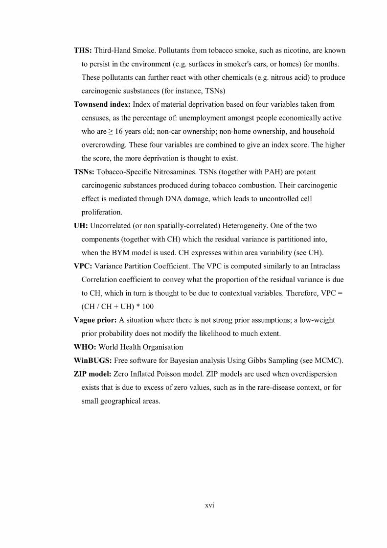
THS: Third-Hand Smoke. Pollutants from tobacco smoke, such as nicotine, are known

to persist in the environment (e.g. surfaces in smoker's cars, or homes) for months.

These pollutants can further react with other chemicals (e.g. nitrous acid) to produce

carcinogenic susbstances (for instance, TSNs)

Townsend index: Index of material deprivation based on four variables taken from

censuses, as the percentage of: unemployment amongst people economically active

who are ≥ 16 years old; non-car ownership; non-home ownership, and household

overcrowding. These four variables are combined to give an index score. The higher

the score, the more deprivation is thought to exist.

TSNs: Tobacco-Specific Nitrosamines. TSNs (together with PAH) are potent

carcinogenic substances produced during tobacco combustion. Their carcinogenic

effect is mediated through DNA damage, which leads to uncontrolled cell

proliferation.

UH: Uncorrelated (or non spatially-correlated) Heterogeneity. One of the two

components (together with CH) which the residual variance is partitioned into,

when the BYM model is used. CH expresses within area variability (see CH).

VPC: Variance Partition Coefficient. The VPC is computed similarly to an Intraclass

Correlation coefficient to convey what the proportion of the residual variance is due

to CH, which in turn is thought to be due to contextual variables. Therefore, VPC =

(CH / CH + UH) * 100

Vague prior: A situation where there is not strong prior assumptions; a low-weight

prior probability does not modify the likelihood to much extent.

WHO: World Health Organisation

WinBUGS: Free software for Bayesian analysis Using Gibbs Sampling (see MCMC).

ZIP model: Zero Inflated Poisson model. ZIP models are used when overdispersion

exists that is due to excess of zero values, such as in the rare-disease context, or for

small geographical areas.

xvii

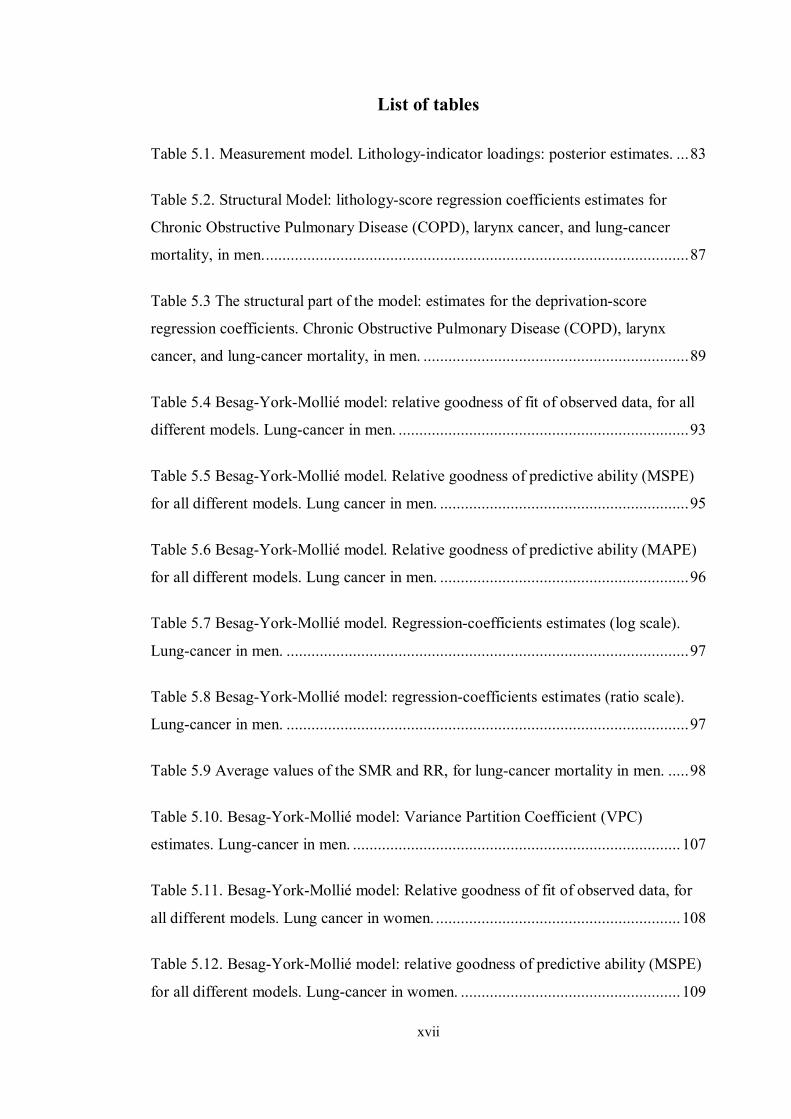
List of tables

Table 5.1. Measurement model. Lithology-indicator loadings: posterior estimates. ... 83

Table 5.2. Structural Model: lithology-score regression coefficients estimates for

Chronic Obstructive Pulmonary Disease (COPD), larynx cancer, and lung-cancer

mortality, in men. ...................................................................................................... 87

Table 5.3 The structural part of the model: estimates for the deprivation-score

regression coefficients. Chronic Obstructive Pulmonary Disease (COPD), larynx

cancer, and lung-cancer mortality, in men. ................................................................ 89

Table 5.4 Besag-York-Mollié model: relative goodness of fit of observed data, for all

different models. Lung-cancer in men. ...................................................................... 93

Table 5.5 Besag-York-Mollié model. Relative goodness of predictive ability (MSPE)

for all different models. Lung cancer in men. ............................................................ 95

Table 5.6 Besag-York-Mollié model. Relative goodness of predictive ability (MAPE)

for all different models. Lung cancer in men. ............................................................ 96

Table 5.7 Besag-York-Mollié model. Regression-coefficients estimates (log scale).

Lung-cancer in men. ................................................................................................. 97

Table 5.8 Besag-York-Mollié model: regression-coefficients estimates (ratio scale).

Lung-cancer in men. ................................................................................................. 97

Table 5.9 Average values of the SMR and RR, for lung-cancer mortality in men. ..... 98

Table 5.10. Besag-York-Mollié model: Variance Partition Coefficient (VPC)

estimates. Lung-cancer in men. ............................................................................... 107

Table 5.11. Besag-York-Mollié model: Relative goodness of fit of observed data, for

all different models. Lung cancer in women. ........................................................... 108

Table 5.12. Besag-York-Mollié model: relative goodness of predictive ability (MSPE)

for all different models. Lung-cancer in women. ..................................................... 109

xviii

Table 5.13. Besag-York-Mollié model: Relative goodness of predictive ability

(MAPE) for the different models. Lung cancer in women. ...................................... 109

Table 5.14. Besag-York-Mollié model: regression coefficients estimates on the log

scale (two upper rows) and ratio scale (two lower rows). Lung-cancer in women. ... 112

Table 5.15. Variance Partition Coefficient: posterior estimates. Lung-cancer in

women. ................................................................................................................... 113

xix

List of figures

Figure 1.1. The Spanish autonomous region of Andalucía (red area). .......................... 1

Figure 1.2. Administrative boundaries of Andalucía. ................................................... 2

Figure 2.1. Main causes of mortality in men. ............................................................. 20

Figure 2.2. Main causes of mortality in women. ........................................................ 21

Figure 2.3. Cancer mortality in men. ......................................................................... 24

Figure 2.4. Cancer mortality in women. .................................................................... 25

Figure 3.1. The Andalusian towns overlaying the lithological map. ........................... 57

Figure 5.1. The measurement part of the model: posterior probability-density

distributions of the lithology-indicator loadings. ....................................................... 84

Figure 5.2. The measurement part of the model: autocorrelation plots and Brooks-

Gelman-Rubin graphs for the lithology-indicator loadings. ....................................... 85

Figure 5.3. The measurement model. Lithology-indicator loadings: history plots. ..... 86

Figure 5.4. The structural part of the model: posterior probability-densities for the

Relative Risk (RR) of mortality explained by the lithology score, in the modelling of

Chronic Obstructive Pulmonary Disease (COPD), larynx cancer and lung cancer, in

men. .......................................................................................................................... 88


relative risk (RR) explained by the deprivation-score. ............................................... 90

Figure 5.6. The structural part of the model: convergence of the deprivation-score

estimates. .................................................................................................................. 91

Figure 5.7. Ranking of posterior estimates of Relative Risk boxplots, for all 101

muncipalities in the province of Almería. Lung-cancer in men. ................................. 99

xx


muncipalities in the province of Cádiz. Lung-cancer in men. ................................... 100


muncipalities in the province of Córdoba. Lung-cancer in men. .............................. 101


muncipalities in the province of Granada. Lung-cancer in men. ............................... 102


muncipalities in the province of Huelva. Lung-cancer in men. ................................ 103


muncipalities in the province of Jaén. Lung-cancer in men. ..................................... 104


muncipalities in the province of Málaga. Lung-cancer in men. ................................ 105


muncipalities in the province of Sevilla. Lung-cancer in men. ................................. 106

Figure 5.16. Besag-York-Mollié model: posterior probability-densities for lithology

and deprivation. Lung-cancer in women. ................................................................. 111

Figure 5.17. Standardised Mortality Ratio estimates for lung-cancer mortality in men.

............................................................................................................................... 114

Figure 5.18. Posterior Relative Risks of lung-cancer mortality in men. .................... 115

Figure 5.19. Exceedance-probabilities map (Probability [Relative Risk > 1]). Lung-

cancer mortality in men. .......................................................................................... 116

Figure 5.20. Exceedance-probabilities map (Probability [Relative Risk < 1]). Lung-


Figure 5.21. Relative Risks explained by lithology scores. Lung-cancer mortality in

men. ........................................................................................................................ 118

xxi

Figure 5.22. Exceedance-probabilities map for lithology scores (Probability [Relative

Risk > 1]). Lung-cancer mortality in men. .............................................................. 119

Figure 5.23. Exceedance-probabilities map for lithology scores (Probability [Relative

Risk < 1]). Lung-cancer mortality in men. .............................................................. 120

Figure 5.24. Relative Risks explained by deprivation scores. Lung-cancer mortality in

men. ........................................................................................................................ 121

Figure 5.25. Exceedance-probabilities map for deprivation scores (Probability

[Relative Risk > 1]). Lung-cancer mortality in men. ............................................... 122


[Relative Risk < 1]). Lung-cancer mortality in men. ............................................... 123

Figure 5.27. Residual Relative Risks. Lung-cancer mortality in men. ...................... 124

Figure 5.28. Exceedance-probabilities map for residual Relative Risks (Probability

[Relative Risk > 1]). Lung-cancer mortality in men. ............................................... 125

Figure 5.29. Exceedance-probabilities map for the residual Relative Risks (Probability

[Relative Risk < 1]). Lung-cancer mortality in men. ............................................... 126

Figure 5.30. Relative Risks explained by spatially Correlated Heterogeneity. Lung-


Figure 5.31. Exceedance-probabilities map for Relative Risks explained by spatially

Correlated Heterogeneity (Probability [Relative Risk > 1]). Lung-cancer mortality in

men. ........................................................................................................................ 128


Correlated Heterogeneity (Probability [Relative Risk < 1]). Lung-cancer mortality in

men. ........................................................................................................................ 129

Figure 5.33. Relative Risks explained by Uncorrelated Heterogeneity. Lung-cancer

mortality in men. ..................................................................................................... 130

xxii

Figure 5.34 Exceedance-probabilities map for Relative Risks explained by

Uncorrelated Heterogeneity (Probability [Relative Risk > 1]). Lung-cancer mortality

in men. .................................................................................................................... 131

Figure 5.35. Exceedance-probabilities map for Relative Risks explained by

Uncorrelated Heterogeneity (Probability [Relative Risk < 1]). Lung-cancer mortality

in men. .................................................................................................................... 131

Figure 5.36. Standardised Mortality Ratios. Lung-cancer mortality in women. ........ 132

Figure 5.37. Posterior Relative Risks of lung-cancer mortality in women. ............... 133


cancer mortality in women. ..................................................................................... 134





Figure 6.1. Pathways in the association of deprivation with lung cancer and radon-gas.

............................................................................................................................... 140

1

Figure 1.1. The Spanish autonomous region of Andalucía (red area).

Chapter 1. Introduction

1.1 Background

Understanding the causes of spatial patterning in the incidence of disease and

mortality is important for both understanding the aetiology of disease, and also in

mitigating their effects [1]. Cumulative evidence from research accomplished in Spain

has shown that there is a pattern of higher mortality rates in the south-west of the

country, due to all-cause as well as certain specific causes. Numerous investigations

dealing with the spatial distribution of mortality have been implemented in Spain over

the last 26 years [2-16]. One conspicuous result of this research is the spatial

patterning in mortality showing higher age-adjusted rates (for both men and women)

in the southern autonomous region of Andalucía. This is the most populated region in

the country (more than 8 million inhabitants, or 18% of the whole Spanish population

[17]) and the second-largest one geographically (87,597 km2

Figure 1.1

, which represents 18% of

the area of the country [18]). shows the geographical location of Andalucía

(own elaboration using QGIS software [19]; the digital Andalusian borders were

obtained from the Andalusian Health Office; countries borders and raster layer were

downloaded from Natural Earth [20]).

2

Spain is divided administratively into 17 autonomous communities, which are further

subdivided into provinces (eight in Andalucía -Figure 1.2) and municipalities [21, 22].

The 1978-1992 Spanish Atlas of Mortality from Cancer [9, p. 19, 214-9, 244] showed

that four of the eight Andalusian provinces (Cádiz, Málaga, Huelva and Sevilla) had

the highest age-adjusted mortality rates among all the Spanish provinces, when

considering neoplasms associated with tobacco smoking and alcohol drinking: cancers

of the lung, larynx, oesophagus and bladder. The male-female ratio was greater than

6:1 for all these causes together. For larynx cancer, the male-female ratio was 38:1.

Furthermore, the province of Cádiz had the highest all-cause age-adjusted mortality

rates: 1,166.65 per 105 inhabitants versus an average value of 951.55 for Spain (or

23% more than average) and 682.8 versus 579.52 in Spain (or 18% more than average)

for men and women, respectively. These differences were even higher when lung

cancer was analysed (91.44 in Cádiz versus 60.16 for Spain, or 52% higher). It is

interesting to note that this pattern of mortality was no longer seen when ill-defined

causes, a measure of data quality regarding mortality analysis, was considered. For

Figure 1.2. Administrative boundaries of Andalucía.

The eight Andalusian provinces –boldface names- overlying the towns borders (own

elaboration using QGIS software).

3

these causes, rates for both men and women were slightly lower than the average value

for Spain.

However, around one third of deaths caused by cancer in men within Andalucía were

due to lung cancer. It is also important to note that lung cancer was responsible for

nearly 30% of Years of Potential Life Lost (YPLL), or premature death due to cancer,

as the mean age at death was 66 years. An atlas from Andalucía for the period 1975-

1997 [23] identified lung cancer as the leading cause of cancer-related mortality for

men with 44,027 deaths for the whole period or 31% of all deaths; in women, it was

the fourth cause of mortality with 4,532 deaths or 6%, in that 22-year period.

Another Spanish small-area mortality analysis, for the period 1987-1995 [10, 11, 13],

also showed the earlier-mentioned pattern of higher mortality rates in the south-west

of the country. The Andalusian provinces of Huelva, Sevilla, Cádiz and Málaga

(Figure 1.2) were revealed as those which accounted for the greatest number of areas

with the highest risk of mortality due to all causes, as well as specific causes including

lung cancer. At a smaller area-level, the Spanish municipal atlas of cancer mortality

for the period 1989-1998 [16], not only confirmed the previous findings on lung

cancer, but also highlighted that the situation had extended to the region of

Extremadura which is situated to the north-west of Andalucía. Furthermore, mortality

due to lung cancer was again shown to be much higher in men residing in the south-

western part of Spain; conversely, the geographical pattern of mortality for women

showed the highest rates in the north-west of the country.

The authors of this Spanish atlas of mortality [16] suggested that the heterogeneity in

the spatial distribution of lung-cancer mortality (by sex) might be related to the

influence of distinct carcinogenic exposures: tobacco smoking for men and radon-gas

for women; although a possible interaction between tobacco smoking and radon-gas

may play a role. The study period targeted by this analysis included mainly cohorts of

women born before the 1940s; that is to say, those who would not yet have massively

acquired the habit of tobacco smoking. The hypothesis of distinct risk factors for men

and women for developing lung cancer was also consistent with a recognised

differential-prevalence in the histological type of tumours [16]: Small Cell Lung

Cancer (SCLC) as well as non-SCLC (squamous-cell carcinoma type) for men; while

non-SCLC (adenocarcinoma type) is more prevalent amongst women.

4

Low socio-economic status (SES) is known to be associated with lower life

expectancy, as well as higher risk for cancer development and poorer survival rates

after diagnosis [24]. The excess of cancer risk in populations with lower socio-

economic status has been consistently shown in many (but not all) countries, for

cancers of the lung and larynx. SES, in turn, is known to vary by small geographical

areas. Therefore, the study of the spatial distribution of SES at area level is relevant in

understanding heterogeneity in the mortality distribution of these cancer sites. Thus,

the 1989-1998 Spanish municipal atlas of cancer mortality [16] showed that all

variables related to SES (including income, illiteracy and unemployment) exhibited a

north-south pattern. This drew attention to Andalucía again, as one of the more

deprived regions of the country. Furthermore, a high variation of SES has been shown

to exist within cities [25-28]. Another ecological study for the period 1987-1995 [29]

found the same north-south geographical pattern for both mortality and deprivation. In

this study, both of two different indices of deprivation were associated with the

geographical distribution of mortality. The so called index I (a summary compound of

social class, unemployment and illiteracy) was associated with mortality in the oldest

group (aged 65 years or more). Index II (comprising overcrowding, unemployment

and illiteracy), was more closely associated with mortality (showing a steeper

gradient) in the youngest group (0-65 year-olds).

Later research on the relationship between deprivation and mortality, for the period

1987-1995 [30] reported a further analysis on the association of the above mentioned

deprivation indices (I and II) with mortality due to different causes. Index I was

associated (amongst others) with Chronic Obstructive Pulmonary Disease (COPD) for

both men and women. Index II was shown to be strongly and positively associated

with mortality due (but not exclusively) to lung cancer and COPD, in men. More

recent research [27] has investigated the relationship between SES and mortality in

Andalucía, at a smaller area-level (census tracts) within the capital cities. A summary

deprivation index (comprising social class, unemployment and illiteracy) showed to be

positively associated with mortality in seven of the eight Andalusian capital cities; this

association was found for both men and women. Within cities, mortality was found to

be higher in more deprived census tracts.

As was mentioned earlier, lower SES has been consistently found to be associated

with higher mortality. Moreover, it has been also associated with higher incidence due

5

to all-malignant tumours and some specific sites (such as lung and larynx cancer),

across different populations and countries [24, 31]. All this has been partially

explained by the association between lower SES with some well-known intermediate

health risks: particularly tobacco smoking, but also lack of physical exercise, alcohol

drinking, as well as occupational and environmental exposures. Tobacco smoking has

been causally associated with a number of cancer sites, such as lung and larynx, but

also with some non-cancer conditions such as COPD. Although lower SES

(deprivation) is usually associated with tobacco smoking, SES also operates through

some other intermediate factors which are not completely understood. For instance,

incidence of lung cancer is higher amongst men with lower SES, even if they are not

smokers [31, 32].

Lower SES has been also associated with poorer survival after diagnosis. This is

relevant not only from a public health perspective, but also from an analytical point of

view; it makes analysis of incidence-data preferred over mortality-data in instances of

low fatality rate [33, p. 65]. Furthermore, SES has been reported to vary across

geography. Hence, concerning the spatial heterogeneity of disease distribution,

geography is thought to serve as a compound surrogate of different factors, such as

lifestyle, environmental exposures, socio-economic characteristics, as well as genetic

traits [1, 14, 34-42]. So, the spatial heterogeneity of distribution of the key

determinants of health could be responsible for distinct geographical patterns of

morbidity and mortality, not only at the international, national, or regional level, but

also at much smaller geographical level like municipalities, and census tracts within

cities.

1.2 Rationale

Understanding why the incidence of disease varies is critical to managing it. Where

spatial patterns occur it is not often easy to explain why. A formal analytical approach

at the individual level is not always feasible. In a spatial context, the information may

not be available, or it may be unlikely to obtain ethical approval. Nowadays,

ecological studies can be used to analyse risk factors for disease, regarding not only

large-scale, but also small-area level populations. Some recent advances have

promoted development of Spatial Epidemiology, e.g. the availability of modern

Geographic Information Systems (GIS) and development of new statistical tools [43-

6

54]; also, computational availability and increased accessibility to routinely collected

data on health-related factors [55, 56]. Some field-related disciplines are especially

relevant to this research area: namely, GIS and Applied Spatial Data Analysis. An

increasing availability of commercial (e.g. ArcGIS) and free software (e.g. GRASS,

GeoDa, R) has provided a means to implement small-area-analysis research. Also,

complex statistical modelling can nowadays be applied to better understand the

heterogeneity of health-status distributions.

In some cases, ready-to-use information includes data regarding socio-economic

characteristics as well as health-related behaviour concerning the study populations,

such as smoking, alcohol drinking and physical activity [57]. In other instances there

is availability of attributes related to the surrounding environment that are thought to

be hazardous and therefore monitored, including chemical products and biological

agents present in drinking water, soil and ambient air [1, 14, 46, 57-59]. For example,

a digitised map exists on lithology that gives detailed information on the rocks

composition, for the Andalusian soils [60]. This allows lithology to be used as a

surrogate measure for potential radon-gas exposure at the small area-level [61]. Other

data sources, such as mortality registries as well as censuses, provide necessary

information with respect to socio-demographic factors. Municipal registries, in Spain,

also provide demographic information on a yearly basis. Therefore, statistical

modelling and disease mapping can provide better identification and interpretation of

health differences among populations [62, 63].

Ecological studies can contribute to the knowledge of the epidemiological features of

the health status of populations, by describing the distribution of their essential

attributes (’person’, ‘place’, and ‘time’). However, area-level analyses on the

significance of risk factors are hindered by potential biases, as well as confounding.

These potential issues can arise from unmeasured variables (frequently SES [1, 34, 64,

65]). The ecological fallacy is especially relevant, where there is a systematic bias

which attributes group-level-characteristics to the individuals. Nevertheless, using

information at small geographical level helps to lessen this bias by making exposure

measurement closer to the individual level [1]. Moreover, current analytical techniques

in statistical modelling allow for different important issues, such as spatial

autocorrelation [63, p. 10], to be addressed. As a result, analysis at the small-area level

has expanded in order to both describe spatial heterogeneity, and determine the main

7

sources of variability. Even though findings at group-level analysis need to be

confirmed at the individual-level, spatial analyses can be hypothesis-generating.

Another important point is whether to use incidence-data or mortality-data. The former

is more appropriate to measure the risk of disease and therefore to establish cause-

effect associations. This is especially the case, when the outcome of interest has a low

fatality rate [33, p. 65]; this hinders mortality from being a good surrogate measure for

incidence, as it may also reflect other influences, some of which may be related to

survival status [66]: thus, accuracy of death-certificate records, health-care

accessibility, prompt diagnosis, treatment availability, or variability in clinical

practice. Notwithstanding all these advantages of incidence-data over mortality-data,

practicality often calls for death-records to be used instead, as they are readily

available. Additionally, that mortality analysis has a long history of major

contributions to the knowledge of cancer epidemiology [33, p. 65-6], although

incidence is preferred whenever is available.

It is also important to bear in mind that mortality data have been widely structured

according to international recommendations by the World Health Organisation (WHO)

[67]. This helps to lessen misclassification problems. In this respect, statistics derived

from death certificates have been reported to underestimate death due to cancer in just

4% of the cases; misclassification is considered to be greater for more difficult

diagnoses such as brain and liver cancer. Therefore, mortality (instead of morbidity)

was considered, given easy accessibility to the Andalusian Mortality Registry.

Reliability of death certificates in Spain is thought to be similar to other countries [68]

for some health events, such as lung cancer. Also, given the high fatality rate of some

conditions (especially lung cancer), mortality would not be much affected by

differentials in survival rates throughout different geographical areas.

In Spain, data from mortality registries is considered to be the only comprehensive

source of information on cancer for the whole country, or at the regional level. Pérez-

Gómez et al. published a review of studies about the quality of data dealing with

mortality due to cancer of different sites, for the period 1980-2002 [69]. The detection

(DR) and confirmation (CR) rates were estimated for different types of cancer.

Clinical and/or pathology data was considered to be the gold standard which death-

certificates information was compared with. DR (or sensitivity) was computed as the

8

conditional probability of cases being classified as cancer by death certificates, given

that they were classified as cancer by the gold standard; that is to say, the probability

of a case being classified as cancer, given that it truly is a cancer case. CR (or positive

predictive value) was calculated as the conditional probability of cases being classified

as cancer by the gold standard, given that they were classified as cancer by death

certificates; that is to say, the probability of a case classified as cancer being a true

cancer case. Accuracy of death certification was considered to be good if both DR and

CR were >= 80%. Over-certification was considered to occur with DR >=80% and CR

<= 80%. Conversely, under-certification was thought to exist if DR <= 80% and CR

>=80%. Cases where both DR and CR were <= 80% were considered to be ill-certified

(low proportion of ill-certification being considered characteristic of a high-quality

standard of information).

Published reports from different cancer registries in Spain, including the one in the

province of Granada (Andalucía), showed that lung cancer mortality had been well

certified during the study period, while larynx cancer had been over-certified [69].

Interestingly, during the 1980s mortality registries at the regional level became

responsible for dealing with these data. During these years, the trend of both ill-

certified tumours and ill-certified non-cancer conditions decreased, while they rose in

1999 (by 31%, for tumours) and then stabilised. The increment in ill-certified cases in

1999 coincided with the introduction of the 10th revision of the International

Classification of Diseases (ICD-10) in Spain. Ill-certification was proportionally

higher (lower quality of data) in women than in men, along all the study period, even

when age-adjusted rates were used.

Some variables, especially age and sex, are well known to account for heterogeneity in

the distribution of overall and cause-specific mortality, among different populations.

To adjust for these potential confounding variables, the Standardised Mortality Ratio

(SMR) has been widely used as a comparison measure. SMR is considered to be a

Maximum Likelihood Estimate of Relative Risk (RR) and is calculated as the ratio of

observed to expected number of cases (O/E) [63, p. 4-5]. Different methods have been

devised to estimate E [51, 70-75] assuming a multiplicative model. The downside of

the SMRs are that in the case of absence of observed cases (which is frequently the

case at the small-area-level), E cannot be computed (so, the ratio is null). Moreover,

estimates can be statistically unstable (small changes in E can produce large variation

9

in SMRs). Given that mortality analysis is concerned with count events, a Poisson

distribution is usually assumed to fit this kind of data [62, p. 314, 76, p. 86, 183-96 ,

77, p. 250, 528-39]. Therefore, the observed number of cases is modelled instead to

give SMR estimates.

The Poisson assumption is supported by the data in some scenarios. Nevertheless,

over-dispersion is a drawback to always bear in mind [44, 77, p. 540-6, 78, p. 21, 114-

6, 320]. In these cases, the data show extra-variability which causes the sampling

distribution not to fit to a theoretical Poisson distribution. This is just one of the

reasons for fitting different models to count-data: e.g. a Negative Binomial or its

Bayesian counterpart, the hierarchical Poisson-Gamma model.

Bayesian modelling offers some advantages over frequentist analysis [79, 80]: Thus,

Bayes’ theorem is, always, the only basic principle used in every analytical situation.

This theorem allows for prior knowledge to be incorporated into the analysis of

current data (also known as the likelihood) to produce direct posterior probability

estimates; these estimates concern the actual dataset being analysed. Conversely, the

frequentist approach resorts to the Null Hypothesis Significance Testing (NHST)

paradigm [81]. In this case, confidence intervals are not related to the actual data

gathered by the researcher. Instead, they are referred to all potential datasets fitting a

theoretical sampling distribution: nothing is assumed about the specific dataset under

analysis [79]. Furthermore, Bayesian analysis usually produces more precise estimates

than those obtained by frequentist methods [82]; this is especially the case when

dealing with small sample sizes. In these situations, Bayesian estimates surpass

frequentist estimates even if the former ones are biased. This is due to larger precision

of the Bayesian estimates, which produce smaller Mean Square Errors (MSE); the

MSE is a frequentist criterion for reliability of estimates, that accounts for both bias

and variance simultaneously [76, p. 164, 82].

Bayesian modelling can be broadly categorised into Empirical Bayes (EB) and Fully

Bayesian (FB) methods. EB methods estimate prior parameters from the data;

conversely, FB methods make use of external information, or assume a range of

plausible values. This is the reason why EB methods do not take into consideration

uncertainty of prior parameters information. FB methods accounts for this potential

source of variability [82]. A whole range of EB models are in use [50, 62, p. 316-21].

10

Some of them (Poisson-Gamma model, Log-Normal, Marshall) shrink SMRs to a

global mean calculated from the data, and some are computationally unstable. To

overcome these problems, Fully Bayesian (FB) methods have been proposed that

make the SMRs to be locally smoothed by taking into account the estimates of

neighbouring areas. Furthermore, some of these hierarchical models (Besag-York-

Mollié [BYM]) allow for covariates to be incorporated [63, ch. 8, 83].

1.3 Main Hypotheses

There is spatial variation in mortality due to lung cancer, COPD and larynx cancer, in

Andalucía. Spatial variation in lung-cancer mortality is dependent on presence of

radon-gas, and area-level deprivation which is a surrogate for smoking. These two

factors may interact; they are also dependent on the lithology which determines the

source of radon and also the deprivation of those residents in the landscape (Figure

6.1).

In contrast, spatial variation in larynx cancer and COPD are dependent on deprivation

(as a surrogate for smoking) but not on radon and the lithology that determines it.

1.4 Secondary hypotheses

Lithology, as a surrogate measure for potential radon-gas exposure, can help to explain

heterogeneity in the spatial distribution of lung cancer mortality.

Lithology cannot help to explain heterogeneity in the spatial distribution of either

larynx cancer or COPD.

1.5 General Aim

To analyse the potential value of lithology in explaining the spatial distribution of lung

cancer mortality in Andalucía, for the period 1986-1995

1.6 Specific objectives

To develop a lithology score, as a surrogate measure for potential radon-gas exposure,

by municipalities in Andalucía

To model the spatial distribution of lung-cancer mortality in Andalucía, using

lithology as a potential explanatory variable, while adjusting for area-level socio-

economic status (SES)

11

To model the spatial distribution of mortality due to larynx cancer and COPD, using

lithology as a potential explanatory variable, while adjusting for area-level SES

To map the distribution of lung cancer mortality in Andalucía as explained by the

whole model, as well as the individual components

1.7 Introduction summary

Several mortality analyses published in Spain have shown that all-causes mortality, as

well as mortality due to some specific diseases such as lung cancer, is higher in the

southern autonomous region of Andalucía. Although this geographical pattern of

mortality has been known for a long time, reasons remain incompletely understood.

Both tobacco smoking and ambient-air pollution by radon-gas have been shown to be

the most important causes of lung cancer mortality. As individual-level information on

these two was unavailable, an ecological study was mandatory. Furthermore, lung

cancer mortality, as well as some risk factors (such as radon-gas exposure), is known

to vary by small geographical areas. The same variation has been reported for SES at

the area-level, which is known to be a surrogate measure for tobacco smoking, while

lithology can be used as a surrogate measure for radon-gas exposure. Spatial

epidemiology at the small-area level is thought to counteract the ecological fallacy;

this is done by producing aggregated measurements that are closer to the individual-

level characteristics than the ones provided by large-scale studies. Geo-referenced data

(at the small-area level) dealing with mortality, population size, SES, and lithology

was available in digital format. Nowadays, GIS software eases the use of spatial data

and current statistical tools (such as the BYM model) can handle some of the

downsides of spatial analysis at the small-area level (instability of rates, spatial

autocorrelation, and excess of zero values).

12

Chapter 2. Literature review

2.1 Aims and strategy

This literature review was intended for retrieving the most relevant scientific literature

concerning the spatial patterning of mortality in Andalucía. The four main areas of

interest were: firstly, current knowledge about main causes of mortality in Andalucía

and their distribution according to place, person and time characteristics; secondly, the

state of the art in small-area analysis in relation to the statistical modelling,

computation and spatial representation of mortality distribution; thirdly, the

epidemiology of lung cancer. Interest was focused on influence and area-level

measurement of tobacco smoking, radon-gas exposure, and SES. In addition, the

epidemiology of larynx cancer and COPD was also reviewed.

Different databases were searched (Medline, Scopus, and Web of Knowledge) and

bibliographic alerts were set up for additional papers to be identified whenever they

cited key articles. Key words for the literature search were identified by means of

Medical Subject Headings (MeSH) thesaurus, which is available through PubMed

online [84]. Some MeSH terms used were ‘small-area analysis’, ‘exp Mortality’,

‘social class’, and ‘socio-economic factors’; also, ‘exp Radon/ae [Adverse Effects]’,

‘Air pollution, Indoor/ae [Adverse Effects]’, and ‘Geographic Information Systems/is,

ut [Instrumentation, Utilization]’. When needed, the literature search was narrowed by

means of MeSH terms which are indicative of quality of study design (i.e. ‘Cohort

Studies’, ‘Case-Control Studies’, or ‘Cross-sectional Studies’). To retrieve relevant

information on the spatial distribution of mortality in Andalucía, various reports were

also accessed online through the Andalusian Health Office website [23, 85, 86]. Some

grey literature was also identified which was significant to the purpose of this review

[51]. Although the bibliographic search was meant to find the most up-to-date

information, some old but highly influential papers were also reviewed [87, 88].

EndNote software [89] was used to store citations together with their respective

articles in PDF format, so that an annotated bibliography could be built and eventually

cited and referenced.

2.2 Overview

The main causes of mortality in Andalucía are reviewed, emphasising the

heterogeneity of its geographical distribution, across the region. Lung cancer mortality

13

is subsequently appraised and the two most important aetiological factors associated

with it (i.e., tobacco smoking and radon exposure) are addressed. Surrogate measures

of potential radon-gas exposure are taken into consideration. Socio-economic status

(SES) is dealt with in some detail, given the relevance of this variable to predict many

different health outcomes. Several indices of area-level deprivation are discussed.

Methodological approaches to the spatial analysis of disease distribution are also

evaluated: the analytical process stresses the need of a hierarchical model and the

advantages and limitations for a Bayesian perspective. Finally, mapping alternatives

are put into the context of current availability of tools for both computation and

representation of spatial data.

2.3 Spatial heterogeneity of mortality in Andalucía

The particular patterning in mortality rates, which shows higher rates in the southern

autonomous region of Andalucía, has been extensively investigated. This pattern is

due to all-cause mortality, as well as specific causes, in both men and women. One

major publication was a comprehensive study authored by López-Abente et al. [9],

who analysed mortality due to cancer and other causes for a 15-year period (1978-

1992). This mortality atlas described patterns of mortality by geographical areas at the

provincial level (52 such areas, plus two autonomous cities, in Spain) and studied

mortality time-trends over three five-year periods, while accounting for a total of

fifteen million deaths which occurred in the whole country. The 1975 and 1986

municipal population registries, as well as the 1981 and 1991 census databases were

used to obtain population data by age and sex. Information on deaths, provided by the

National Statistics Institute of Spain, was classified using the 9th revision of the

International Classification of Diseases (ICD-9). Mortality rates were adjusted by the

direct method using the standard European population, given similarities with the age-

structure of the Spanish population. Poisson regression analysis was used to model the

observed number of cases while accounting for age, geographical area, and time-

period. Interestingly, mortality rates due to some cancer sites associated with tobacco

smoking and alcohol drinking (lung, bladder, larynx and oesophagus) were highest in

the west of Andalucía; especially in the province of Cádiz, but also in those of Málaga,

Huelva, and Sevilla. The male-female ratio was 6:1 for lung cancer and 38:1 for larynx

cancer. This indicates distinct lifestyles between Spanish men and women, at that

time, concerning exposure to the main risk factors. The authors also found that

14

mortality rates due to diabetes and cardiovascular diseases were highest, as well, in

western Andalucía. This geographical study was not a small-area analysis and did not

take into account potential overdispersion due to spatial autocorrelation, or excess of

zero values; if overdispersion had been present, too narrow confidence intervals (or

credible intervals, if a Bayesian analysis had been used) would have been obtained,

which would have led to false alarms [90]. However, this study by López-Abente et al.

[9] produced a very comprehensive mortality atlas that uncovered many different

mortality patterns, on numerous diseases. Moreover, in a further study [16] at a much

smaller area level (see pg. 25) this author confirmed the same results by means of a

Bayesian model that took overdispersion into consideration.

Ischaemic heart disease (heart attack) was also studied at the provincial level to

analyse mortality during two four-year periods (1988-1991 and 1994-1997) in Spain.

Boix-Martínez et al. [12] analysed mortality data provided by the National Statistical

Institute of Spain, while population data were computed by the authors using

interpolation methods on census data. Log-linear Poisson regression was used to

estimate time-trends while adjusting for age. Smoothing techniques were not applied,

nor was socio-economic status accounted for. A decreasing time-trend in mortality due

to ischaemic heart disease was found in Spain between the two study periods. Overall

mortality rates in Spain were second lowest (after France) when compared with

mortality rates of all European countries. Nevertheless, high spatial variation was

observed within the country. Andalucía was amongst the regions with higher mortality

rates, especially in the provinces of Sevilla and Cádiz.

A subsequent study by Ramis-Prieto et al. [91] undertook a spatial analysis at a

smaller geographical unit of analysis: 8077 municipalities were analysed to study the

geographical distribution of haematological neoplasms. These malignancies included

leukaemia, non-Hodgkin's lymphoma (NHL) and multiple myeloma. Data on cases for

the period 1989-1998 were provided by the National Statistics Institute of Spain, and

population data by age and sex were obtained from the 1991 census and 1996

municipal registries. Standardised Mortality Ratios (SMRs) were computed by the

indirect method, using the whole Spanish population as the source of rates (internal

standardisation) by age-group and sex. Three different Bayesian hierarchical models

were compared: The BYM model (section 5.3) [92], the Zero Inflated Poisson [44, 90,

93] (ZIP) (see pg. 67) model and Lawson's mixtures model [94]. All three gave

15

similar results, the BYM model being the more conservative one as it caused fewer

false alarms; that is to say, Relative Risks (RRs) estimates were less frequently higher

than 1 that is raw SMRs were not indicative of an excess in risk. Highest RRs were

estimated in municipalities within Barcelona province (northern Spain) as well as the

Canary Islands. With regard to Andalucía, the western cities of San Juan de

Aznalfarache, Huelva, and Sevilla showed the highest risks. In eastern Andalucía, it

was the city of Granada which emerged as a high risk area for haematological

malignancies. The authors concluded that this concentration of risk in highly urbanised

areas could be explained by environmental factors in relation to industrialisation, as

this is the case for western Andalusian provinces. According to the authors, an

alternative aetiological hypothesis that associates childhood leukaemia with common

infections and population mixing [36] would be plausible in Barcelona. Nevertheless,

the observed geographical pattern was only due to mortality in older age-groups.

Another small-area analysis at the municipal level was carried out by Aragonés-Sanz

et al. [95] to investigate the geographical distribution of mortality due to cancer of the

oesophagus in Spain during the period 1989-1999. The 1991 census and 1996

municipal registries were used to obtain population data by age and sex. The SMRs

were computed using the indirect method; the overall Spanish population (internal

standardisation) provided the rates to compute the expected number of cases. The

authors used Bayesian analysis by means of the BYM model to smooth the RRs

estimates. An excess risk was found amongst men residing in, but not only,

municipalities in the provinces of Cádiz and Sevilla, in western Andalucía.

Conversely, an excess of risk was found for women in the south-east of Andalucía

(Málaga and Granada). The authors attributed this spatial heterogeneity in risk by

sexes to differences in the distribution of some risk factors such as tobacco smoking,

alcohol drinking, obesity, and diet. They recommended that future studies should

account for socio-economic status, as a surrogate measure for exposure to various risk

factors: low socio-economic level has been associated with higher rates of

oesophageal cancer, as well as other cancer sites [95]. With regard to cancer of the

oesophagus, this association was thought to be due to higher levels of tobacco

smoking and alcohol consumption in people of lower socio-economic status. In

addition, people in lower socio-economic strata tend to live in more polluted areas,

follow less healthy diets, and have more difficulties in accessing health services.

16

Another Spanish atlas of mortality, at a smaller geographical level than the previous

one [2], was produced by Benach et al. [11]. They studied mortality due to 14 different

causes of death in 2218 small-areas in Spain, during the period 1987-1995. The units

of analysis were constructed by GIS software using municipalities (8077 according to

the 1991 census) as the building structure; these new small-areas had a minimum of

3500 inhabitants to preserve confidentiality, in agreement with the National Statistical

Institute of Spain. For this same reason, deaths were aggregated over a nine-year

period. Socio-demographic data were also obtained from the census. The expected

numbers of cases were computed by means of Indirect, internal standardisation.

Empirical Bayes analysis was used to compute RR estimates. The authors considered

that data from mortality registries were the most important source of information for

small-area analysis in Spain. This was not only due to ready availability of

information, but also because the quality of death certificates in Spain was considered

to be of a similar standard compared with other European countries. In this paper, the

authors published results concerning lung cancer as well as breast cancer. Andalucía

was one of the four Spanish autonomous regions (out of 17) with highest mortality

rates due to lung cancer. An excess of risk was detected in areas within the provinces

of Huelva, Sevilla, Cádiz and Málaga (western Andalucía). This excess of risk was

found for both age-groups studied, people less than 65 years old, and age 65 years and

older. Most high risk areas for breast cancer were concentrated in Cataluña (northern

Spain). However, areas within some western provinces of Andalucía (Cádiz and

Sevilla) also showed excess mortality risk. The authors considered the inclusion of

socio-economic and environmental indicators to be of major importance in future

research to help explain this spatial variation in risk of death. This small-area analysis

published by Benach et al. [11] used EB analysis, instead of FB methods as was the

case in the study by López-Abente et al. [16]; interestingly, both studies (which

analysed overlapping periods of time, 1987-1995 and 1989-1998, respectively) found

the same spatial patterning of higher mortality in western Andalucía. However, none

of them either formally tested any hypothesis about exposure to potential risk factors,

or adjusted for any confounders other than age. Later research on small-area analysis

[96] confirmed these results (although confined to people aged 65 years and older)

during the whole period 1981-2006.

17

More recently, Ocaña-Riola et al. [15, 27] addressed an ecological study to analyse the

association between deprivation and all-cause mortality for the period 1992-2002.

These researchers used the smallest geographical units of analysis readily available:

census-tracks (between 500 and 2000 inhabitants). The capital cities of Andalucía

(southern Spain) and Cataluña (northern Spain) were studied so that regions with

different levels of deprivation could be compared; at that time, per capita income in

Cataluña was 54% higher than in Andalucía. Information on deaths was supplied by

the Regional Ministry of Health in each of the two autonomous regions. The 1991

census was used to obtain population data. Principal Component Factor Analysis

(PCFA) was used to derive an area-deprivation index comprised of the percentage of

manual workers, unemployment and illiteracy. A BYM was fitted to the observed

number of cases, via Markov Chain Monte Carlo methods (MCMC). Results for men

showed higher mortality rates in more deprived areas of both Andalucía and Cataluña.

However, this pattern was not so obvious for mortality in women in either region.

These consistent results through very different socio-cultural contexts suggest that this

deprivation index is appropriate to measure socio-economic differences at the area-

level in Spain, at least in men. The results were also in agreement with previous

research using this same deprivation index at the provincial or municipality level.

After adjusting for deprivation, residual (not explained by the model) variation was

mainly due to the spatially-structured component in the model. This finding was

attributed by the authors to contextual effects. These were considered to be area-level

(neighbourhood) characteristics that might be related to deprivation, especially in

women, which would explain differences between sexes. Another interesting

characteristic of this study is the use of the smallest spatial units of analysis (census-

tracks). The association found in this study [15, 27] between the index of deprivation

and mortality, and the fact that this index worked well in distinct socio-economic

settings, provided a useful measure of deprivation for using in the analysis of spatial

epidemiology in Spain.

There has also been considerable research on the relationship of health events

(particularly different types of cancers) with putative environmental risk factors. One

of these studies, by López-Abente et al. [97], carried out a spatial point-source analysis

in relation to mortality due to cancer. The aim was to analyse Spanish towns close to

nuclear power plants and nuclear fuel facilities, for the period 1975-1993. Log-linear

18

models were used and socio-demographic variables at the area-level (such as income,

unemployment and illiteracy) were accounted for. "Near versus far" comparisons were

used to analyse differences between exposed and unexposed towns, while adjusting for

population size and deprivation at the area-level. An excess of risk was detected for

mortality due to lung and renal cancers in towns nearby nuclear fuel facilities. The

authors recommended monitoring of incidence and mortality in areas close to health-

hazard facilities. In this study [97] the number of deaths was modelled while allowing

for important covariates (deprivation and population size); overdispersion was also

accounted for. An interesting result was the association between residence nearby

nuclear fuel facilities, and lung-cancer mortality. Although relevant, this finding

cannot explain the characteristic patterning of higher mortality in western Andalucía;

there is just one such facility in the region, which is located in the province of Córdoba

(Figure 1.2). In addition, the exposure area that was considered to be biologically

plausible was only 30 km around the plant.

Another ecological study at the municipal level (López-Abente et al. [98]) assessed the

link between environmental factors associated with farm-related activities, such as

pesticides, and mortality due to brain cancer in northern Spain. This study highlighted

the suitability of small-area analysis using Bayesian hierarchical models to allow for

true mortality patterns to emerge. Furthermore, Bayesian hierarchical models, such as

BYM that include a spatial auto-correlated term, help in accounting for residual

variation in risk. This residual variance is considered to be due to unmeasured risk

factors which are linked to geography (contextual effects).

Putative environmental factors responsible for cardiovascular diseases have been also

investigated. In this way, Ferrándiz et al. [14, 99] analysed influence of water hardness

(due to presence of calcium and magnesium) in relation to mortality risk from

cardiovascular diseases, for the period 1991-1998. Both cerebrovascular disease

(stroke) and ischaemic heart disease (heart attack) were studied. This was a small-area

analysis at the municipal level in the autonomous region of Valencia (eastern Spain).

Indirect, internal standardisation was used to compute expected number of cases, using

the overall population of interest as the source for the rates. An Empirical Bayes (EB)

hierarchical Poisson-gamma model was use to fit the data (see pg. 144). The authors

took into account deprivation at the area-level, by means of an index comprised of the

percentage of illiterate and unemployed people, as well as the number of vehicles per

19

person. They found a weak U-shaped protective effect of magnesium concentration in

drinking water, from mortality due to cardiovascular diseases. That is to say,

magnesium seems to be protective at medium concentrations, which the authors found

to be in agreement with previous research in France. This study highlights suitability

of ecological studies to address research concerning small environmental risks which,

in addition, show slight spatial variations.

2.4 Main causes of mortality

Cardiovascular diseases and cancer of different sites were the most important causes

of mortality for both men and women residing in Andalucía, during the 22-year period

spanning from 1975 to 1997. Amongst all cancer sites, lung cancer was the leading

cause of mortality, with a total of 48,559 deaths (or 25.8% of all deaths due to cancer

[23]). Figure 2.1, Figure 2.2, Figure 2.3, and Figure 2.4 (own elaboration with data

from the Andalusian Health Office) show information obtained from a study

accomplished for the period 1975-1997 [23]. The geographical units of analysis used

in this study were Primary Health Care Districts (PHCD), whose population ranged in

size from 11,000 to 300,000 inhabitants in the year 1988. Information on deaths

included in this study was provided by the National Statistical Institute of Spain for the

period 1975-1991 and by the Andalusian Statistical Institute for the period 1992-1997.

Data on sex, age, and year of death were analysed according to the 8th revision of the

International classification of diseases (ICD) for the first period, while the ICD-9th

revision was used to classify deaths for the second period. Crude rates, as well as age-

adjusted ones were computed; for the latter ones, the European population was used as

a reference source to obtain the expected number of cases. SMRs were also obtained

using indirect, internal standardisation; in this case, the overall Andalusian population

was used as source for the rates to derive the expected numbers of cases. Years of

Potential Life Lost and percentage of change (year-to-year, and first-to last-five year

periods) were calculated for cancer, cardiovascular diseases (CVD), diabetes, traffic

accidents and other causes. Deprivation was, nevertheless, not accounted for.

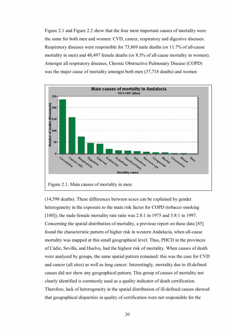
20

Figure 2.1 and Figure 2.2 show that the four most important causes of mortality were

the same for both men and women: CVD, cancer, respiratory and digestive diseases.

Respiratory diseases were responsible for 73,869 male deaths (or 11.7% of all-cause

mortality in men) and 48,497 female deaths (or 8.5% of all-cause mortality in women).

Amongst all respiratory diseases, Chronic Obstructive Pulmonary Disease (COPD)

was the major cause of mortality amongst both men (37,718 deaths) and women

(14,598 deaths). These differences between sexes can be explained by gender

heterogeneity in the exposure to the main risk factor for COPD (tobacco smoking

[100]); the male-female mortality rate ratio was 2.8:1 in 1975 and 5.8:1 in 1997.

Concerning the spatial distribution of mortality, a previous report on these data [85]

found the characteristic pattern of higher risk in western Andalucía, when all-cause

mortality was mapped at this small geographical level. Thus, PHCD in the provinces

of Cádiz, Sevilla, and Huelva, had the highest risk of mortality. When causes of death

were analysed by groups, the same spatial pattern remained: this was the case for CVD

and cancer (all sites) as well as lung cancer. Interestingly, mortality due to ill-defined

causes did not show any geographical pattern. This group of causes of mortality not

clearly identified is commonly used as a quality indicator of death certification.

Therefore, lack of heterogeneity in the spatial distribution of ill-defined causes showed

that geographical disparities in quality of certification were not responsible for the

Figure 2.1. Main causes of mortality in men.

21

geographical pattern in mortality. Only a small proportion of deaths were recorded

under this category for both men and women: 2.2% and 3.3%, respectively.

Many risk factors (including tobacco smoking, obesity, arterial hypertension, low rates

of physical activity, poor diet, heterogeneity in access to health-care services and

quality of health care) have been studied with an aim of explaining geographical

disparities in mortality. Also SES, at the individual or area level, has been considered

because of its predictive value as a surrogate measure for risk factors exposure.

Nevertheless, known risk factors and socio-economic determinants, as studied to date,

are only considered to account for a small fraction of the known variability. Although

not completely understood, environmental, social and occupational factors have been

also suggested that should be related to this mortality pattern. Thus, an editorial

published by Benach [10], highlighted the pattern of higher mortality in western

Andalucía, during the period 1987-1995: only 8% of the Spanish population lived in

the provinces of Cádiz, Huelva and Sevilla. In contrast, one third of all deaths in

Spanish high-risk mortality areas occurred in towns within these three provinces.

Occupational, environmental and socio-economic factors were considered worthy of

further investigation, as up-to-date knowledge had not provided a complete answer to

this public health issue.

In addition, some components of SES seem to play an important role in this striking

pattern of geographical disparity: namely illiteracy, unemployment and overcrowding.

Figure 2.2. Main causes of mortality in women.

22

Moreover, some already known risk factors, such as tobacco smoking, are strongly

related to SES [24, 31]. This strong dependency between SES and tobacco smoking

led Escolar-Pujolar [101] to think that the relevance of factors responsible for this

geographical pattern of higher mortality in south-western Spain has varied with time.

Based on the Atlas of Mortality in the Province of Cádiz for the period 1975-1979, the

author concluded that this mortality pattern already existed before current industries

started operating in the province. Neither petrochemical plants nor manufacturing

industries such as cellulose, gas, steel, or thermal power stations operated before 1967.

The author hypothesised that no single factor was responsible for this mortality pattern

and causes are probably changing across time. Therefore, higher mortality observed in

the area of ‘Campo de Gibraltar’ (towns of Jimena de la frontera, Castellar de la

frontera, San Roque, La Línea, Los Barrios, Algeciras and Tarifa) was thought to be

mediated by poverty and tobacco exposure. Poverty, acting as a surrogate measure for

exposure to various risk factors, could explain the excess of mortality due to cancer of

different sites. Low SES has been associated with worse living conditions and less

healthy life-style (including higher rates of tobacco smoking). According to the author,

this was the case in Campo de Gibraltar for many decades before the study period

(1975-1979) while new environmental hazards may contribute to the excess mortality

which occurred afterwards. That deprivation may play a substantial role in the spatial

distribution of mortality in Andalucía is in accord with an earlier small-area analysis

by Benach et al. [7]; the spatial distribution of a deprivation index (that comprised

unemployment, illiteracy, and overcrowding) was shown to mimic that of higher

mortality rates in western Andalusian municipalities.

Tomatis [31] showed, in a review paper, how lower SES is related to higher incidence

and mortality due to differing cancer. Thus, lung and larynx cancer are amongst the

tumours for which this differential has been found to be greatest. SES is considered to

be an intermediate factor between different kinds of exposures and disease incidence

and mortality. Many different variables are in use to measure SES. For instance, lower

education is associated with worse living and working conditions, material

deprivation, and less healthy life-styles. Furthermore, education seems to be a better

predictor (of incidence and mortality due to cancer) than occupation. Exposure

differences between people of high and low SES are related to well-known

aetiological risk factors, such as tobacco smoking and alcohol drinking, which are

23

more frequent amongst people of lower SES. Nevertheless, these risk factors cannot

completely explain differences in mortality. Hence, the residual higher risk remaining

in lower SES groups when analysing lung cancer, even after adjusting for tobacco

smoking habit. This review [31] highlights the need of accounting for deprivation in

small-area studies, as this covariate is not only a surrogate measure (and a potential

confounder) for tobacco smoking [102], but also for many other exposures [103].

Kogevinas et al. [24, 66] also reviewed the association between SES and cancer. An

excessive incidence of and mortality from respiratory cancers (lung, larynx, and nose)

has been reported in men of lower SES; there is also an excess of risk, in people of

lower SES, for tumours of the mouth, pharynx, oesophagus, stomach, and cancer as a

whole, in different populations from various countries. Conversely, higher SES has

been associated with some other cancer sites (colon, brain and skin). Tobacco smoking

has been aetiologically associated with cancer of different sites, especially lung,

larynx, mouth, pharynx and bladder. In most industrialised countries (including Spain)

rates of tobacco smoking are higher in people of lower social class and these

differences are greatest amongst men. Occupation is another important intermediate

factor frequently measured as a component variable of SES, as manual workers tend to

be more frequently exposed to hazardous substances with carcinogenic effect. An

excess of risk for cancer development and mortality has also been associated with

unemployment. Interestingly, this risk remains after tobacco smoking, social class and

alcohol drinking are accounted for. Exposure to environmental factors is also mediated

by SES; some evidence suggests that people of lower SES are more frequently

exposed to certain air pollutants, which in turn is a risk factor for lung cancer [103,

104]. Notwithstanding this link between deprivation and exposure to environmental

pollutants, recent research has shown that this association can be either positive or

negative, depending on the environmental factor under consideration. As an opposite

example to tobacco smoking, a negative association has been shown to exist between

deprivation and radon-gas exposure; that is to say, people residing in less deprived

areas have been found to be more exposed to radon-gas [103].

Amongst various mortality causes due to different cancer sites, lung cancer was

identified as the leading cause of cancer-related mortality for men, in the report

published by the Andalusian Health Office for the period 1975-1997 [23]. With age-

standardised rates of 81 deaths per 100,000 men, 44,027 cases (or 30.4% of all male

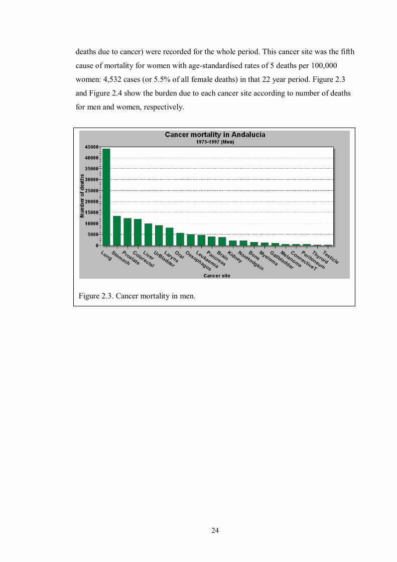
24

deaths due to cancer) were recorded for the whole period. This cancer site was the fifth

cause of mortality for women with age-standardised rates of 5 deaths per 100,000

women: 4,532 cases (or 5.5% of all female deaths) in that 22 year period. Figure 2.3

and Figure 2.4 show the burden due to each cancer site according to number of deaths

for men and women, respectively.

Figure 2.3. Cancer mortality in men.

25

A small-area analysis at the municipal level (8,000 Spanish towns) was published by

López-Abente et al. [16] for a period (1989-1998) overlapping that of the report by the

Andalusian Health Office (1975-1997) [23]. Poisson log-linear hierarchical regression

models were used to account for spatial autocorrelation, which is an important source

of overdispersion in models dealing with counting data. Specifically, the BYM model

was used. Updated information on lung cancer was provided by the authors who

highlighted that this tumour still had, in 2004, a very poor prognosis (only a five-year

12% age-adjusted survival rate) and was the most frequent malignancy in men (28%

of mortality due to neoplasms); in women lung cancer caused 5% of all deaths due to

cancer. According to the authors, age-adjusted rates in men reached maximum levels

in 1995 and then declined. Conversely, age-adjusted rates in women started to rise at

the end of the 1980s. The authors observed specific cohort effects in women: those

born before 1917 experienced a progressive increment in risk; mortality decreased

then in women born before 1940 and risk rose again for birth cohorts born after 1940,

in parallel with tobacco smoking consumption amongst women. This led the authors to

hypothesise that a lung cancer epidemic in women could be expected.

The characteristic geographical pattern was again found in this small-area analysis:

mortality due to lung cancer was higher in towns in south-western Spain (provinces of

Cádiz, Huelva, Málaga, and Sevilla). However, this pattern previously observed had

Figure 2.4. Cancer mortality in women.

26

been extended during this study period (1989-1998) to the adjacent autonomous

community of Extremadura, to the northwest of Andalucía. As the geographical unit of

analysis (towns) was smaller than the one used in previous studies (provinces) the

authors could describe in more detail how towns on the coast line had the highest rates

in known high-risk provinces. This finding was attributed to higher urbanisation of

those municipalities. The authors considered of special interest mapping of lung

cancer mortality in women, given that mortality in this period was mainly represented

by birth-cohorts older than the generation born after 1940, when Spanish women

massively acquired the habit of tobacco smoking. Therefore, risk factors (e.g.

environmental exposures) other than tobacco smoking could be responsible for any

geographical pattern in women’s mortality. Thus, the high mortality rates also

observed in north-west Spain (autonomous region of Galicia) were considered to be

potentially associated with radon-gas exposure; these conclusions were supported by

high levels of radon-gas detected in this area. On the other hand, high rates in

Barcelona (north-east Spain) were presumed to be due to industrial pollution.

Nevertheless, no hypothesis (other than urbanisation) was offered for the high rates

observed in towns of south-western Andalucía.

Additionally, the authors claimed that distinct risk factors could be responsible for

differences between men and women. This hypothesis was based on distinct

histological types usually found between sexes: squamous-cell carcinoma and SCLC,

which are strongly related to tobacco smoking, are more frequent in men. In contrast,

adenocarcinoma is more commonly diagnosed in women. Another cancer site, larynx,

was also found to have a geographical pattern of mortality similar to that of lung

cancer. Larynx cancer has been causally associated with tobacco smoking (and alcohol

intake). In 2004, Spain was the European country with the highest incidence and

mortality due to larynx cancer, in men. Conversely, in women, incidence and mortality

rates due to larynx cancer was amongst the lowest in Europe. In Andalucía, the

provinces of Huelva, Sevilla, and Cádiz showed the highest mortality rates, similar to

rates of mortality due to lung cancer. However, unlike lung cancer, larynx cancer

showed a high age-adjusted survival rate (60% five-year survivorship).

2.4.1 Aetiology and epidemiology of lung cancer

One of the earliest investigations into the association between tobacco smoking and

carcinoma of the lung was a case-control study published by Doll and Hill [87], that

27

compared more than 2,000 hospitalised patients; cases had been diagnosed of cancer

of the lung, stomach and large bowel, while a second group of patients with diagnoses

other than cancer were used as controls. A much larger proportion of smokers were

found amongst lung cancer patients than control. Also, a dose-response relationship

between tobacco smoking and lung cancer was found, although no differences were

found, for the effect of smoking, between those that inhaled and did not inhale the

smoke, a finding that the authors could not explain. At that time, arsenic was the only

known substance present in tobacco manufactures thought to have a possible (but not

yet proved) carcinogenic effect. In this study [87], no association was found between

tobacco smoking and incidence of cancer other than lung cancer or non-cancer

diseases (including other respiratory conditions and cardiovascular diseases).

The authors were very cautious about drawing any conclusions concerning a potential

causal association between smoking and lung cancer, given the weak biological

plausibility of such a relationship at that time. Nevertheless, this case control study

was carefully designed and analysed: subjects were comparable as they were all

recruited from the same setting (hospitalised patients). Lack of any associations

between tobacco smoking and diseases other than lung cancer, as well as with the

smoking pattern (smoke inhalation) would be afterwards contradicted by the analysis

of a large cohort-study also published by Doll [105, 106]. This disagreement in the

results between both studies could have been due to the small number of cases

analysed in the case-control study, as compared with the cohort study (2,475 vs.

34,439). An ample group of people were studied that suffered from different diseases,

including cancer sites other than lung, which was useful to counteract any differences

attributable to recall bias. The finding of a dose-response relationship (drawn by

means of a detailed and structured smoking history) supported the tenet of a causal

relationship between tobacco smoking and lung cancer.

Tobacco smoking has been causally associated not only with cancer of the lung but

also with cancer that affects other close organs such as the mouth, pharynx, larynx and

oesophagus, as well as distant ones such as bladder and kidney. Contrary to the state

of knowledge at the time when Doll and Hill accomplished their case-control study in

1950 [87], nowadays it is known that tobacco smoking entails exposure to thousands

of substances, 100 of which, at least, are known to have possible carcinogenic effect

[107]. According to a review by Shields [108], one of the most important carcinogenic

28

substances present in tobacco smoke are tobacco-specific nitrosamines (TSNs) as the

concentration of this substance in tobacco manufacturing has increased. In contrast to

TSNs, nicotine (which is responsible for addiction to tobacco smoking) has decreased

with time. This has, in turn, led smokers to consume more cigarettes and to inhale

smoke more deeply so that they are able to maintain nicotine concentration in their

blood and thus avoid abstinence syndrome [108].

The mechanism by which TSNs contribute to develop lung cancer (as well as cancer

of other sites) is well understood [107, 108]. TSNs are formed during the process of

tobacco manufacturing and are known to induce deoxyribonucleic acid (DNA) damage

by forming different types of chemical adducts. As DNA contained within cell nuclei

is responsible for the genetic information involved in cell replication, alteration of this

process leads to uncontrolled reproduction of organ cells, which initiates

carcinogenesis. The ultimate mechanism by which carcinogenic substances present in

tobacco smoke exert their effect seems to be mediated by interfering with DNA repair

through gene mutations. The level of exposure to these carcinogenic substances

present in tobacco smoke seems to be determined by the individual smoking habit of

each tobacco user: firstly, the lifespan of the habit and number of cigarettes smoked

per day; secondly, the type of cigarettes consumed as composition varies between

brands and thirdly, the way cigarettes are consumed (e.g. the depth of inhalation and

frequency). Individual susceptibility is also thought to play an important role in

determining cancer risk [108]. Thus, increased susceptibility to mutagenic effects has

been found in lung cancer patients that were smokers.

Differences in cancer risk are also known to exist between sexes. Men tend to suffer

from SCLC, while adenocarcinoma is more frequently diagnosed in women;

moreover, women have twice as high a risk as men. Some researchers have

hypothesised that these differences between sexes could be related to exposure to

different environmental carcinogens: tobacco smoke for men and radon-gas for

women [16]. Alternatively, Shields proposed that these differences could be due to

different smoking patterns [108]. Hence, women would be exposed to greater

concentrations of TSNs as they acquired the tobacco habit more recently, i.e., when

cigarettes already had higher concentrations of this carcinogenic substance. There is

also evidence of higher levels of DNA adducts mediated by other chemical

compounds, such as Polycyclic Aromatic Hydrocarbons (PAH), in women, which

29

supports the hypothesis that women are more susceptible to the adverse effects of

tobacco smoking.

Alberg et al. published a comprehensive review on the aetiology of lung cancer. In this

paper, the authors claimed that both epidemiological and biological evidence have

undisputedly established the causal relationship between tobacco smoking and lung

cancer [109]. Moreover, tobacco smoking is considered to be responsible for more

than 90% of all lung cancer cases. This association between tobacco smoking and lung

cancer had been found in many case-control studies [87, 110] in the UK and the USA

(amongst other countries) in the 1950s and was later on confirmed by large studies

such as the British doctors’ cohort study by Doll et al. [87, 111] that followed a cohort

of more than 34,000 British male doctors for a 50-year period (1951-2001). Data on

participants' habits were periodically assessed. This study provided new insight into

tobacco smoking and mortality due to cancer of different sites. Tobacco smoking was

associated not only with lung cancer but with many other cancer sites, such as oral and

nasal cavities, sinuses, larynx, oesophagus, liver, stomach, pancreas, kidney, bladder,

uterus, and with myeloid leukaemia [111]. Although only one in ten smokers suffers

from lung cancer, 50% of the smokers die prematurely from a tobacco-related disease.

This study showed that a smoker’s life expectancy is reduced by 20 years as compared

to a non-smoker. Nevertheless, quitting smoking at any age partially reduces this

difference between smokers and non smokers. Results from the study by Doll et al.

[87, 106] were closely in agreement with a review by the International Agency for

Research on Cancer (IARC) concerning the carcinogenic effect of tobacco smoke

[112]. This study found a positive association between tobacco smoking and cancer of

28 different sites; for these types of cancer, a dose-response relationship with tobacco

smoking was also found.

It has been shown that smokers have a 20-fold increase in risk for lung cancer

compared to non-smokers [109]. Furthermore, rates of tobacco smoking predict those

of lung cancer 20 years later. Amongst the main determinants, duration of the smoking

habit is now considered to be the most relevant predictor of lung cancer development,

over and above the number of cigarettes smoked. Although quitting smoking is always

beneficial, risk in ex-smokers remains higher than in never-smokers for more than 40

years after the habit has been abandoned [109]. Research in molecular epidemiology

[107, 113] has found that individual susceptibility is associated with gene-environment

30

interaction that may determine heterogeneity of outcomes after exposure to similar

levels of tobacco smoke.

Thus, gene-environment interaction can modulate factors such as metabolism of

carcinogenic substances and production of DNA adducts [107, 108], which is thought

to also underlie race and sex differences for susceptibility to tobacco smoke, as well as

patterns of smoking behaviour (mediated by dopamine receptors in the brain). These

patterns can explain why changes introduced in cigarette manufacturing in the 1950s

(such as low tar and low nicotine, as well as filtered cigarettes) that were thought in

the past to entail a lower risk for lung cancer, caused exactly the opposite effect. Doll

et al. [106] compared risk of mortality within the cohort of British physicians between

the two 20-year periods and showed a higher risk of mortality for the second half of

the follow-up period. This has been explained by changes in the smoking pattern due

to lower content of nicotine and higher content of TSNs present in cigarettes

manufactured since 1950.

Some epidemiological reviews [107] have included cohort studies which have shown

that tobacco smoke is associated with lung cancer, in non-smokers who are passively

exposed to tobacco smoke. Thus, it has been reported that non-smokers who were

married to smokers had a 20% increase in lung cancer risk [109]. Although a dose-

response relationship between tobacco smoking and lung cancer has been shown to

exist, it is interesting to note that a threshold level seems not to exist; that is to say,

some risk still remains even at levels of exposure much lower than those experienced

by active smokers. It is considered by some authors [107-109] that tobacco smoke can

lead to different histological types of cancer: the more common ones are squamous-

cell carcinoma, adenocarcinoma, and SCLC, while others [16, 114] have hypothesised

that these differences can be the result of distinct environmental exposures (such as

radon-gas).

Many environmental factors other than tobacco smoke have also been associated with

lung cancer. Thus, occupational factors such as arsenic, chromium, nickel and asbestos

(the last one interacting synergistically, in a multiplicative way, with tobacco smoke)

cause lung cancer [109]. Ionizing radiation is also known to be a risk factor to develop

lung cancer. This is the case for High Linear Energy Transmission (LET) radiation,

such as radiation from radon-gas exposure, which produces more organ damage than

low-LET radiation (e.g. x-rays) [109]. Radon-gas is known to emit alpha particles that

31

cause permanent damage of tissues in organs. As for tobacco smoke, a non-threshold

dose-response relationship is thought to exist between exposure to radon-gas and lung

cancer [115]. Radon is now considered to be second to tobacco smoke in the number

of lung cancer cases attributable to exposure to environmental factors [116]. Radon-

gas has been considered to be responsible for 10% of all lung cancer cases in the US

[117]. It is considered that tobacco smoke can act synergistically with other factors to

initiate or promote lung cancer. For instance, it is thought that tobacco smoke and

radon-gas exposure have a supra-additive (but not multiplicative) effect for lung

cancer risk [114].

Indoor air pollution due to both second-hand tobacco smoke and radon-gas exposure

are considered to be the most important environmental risk factors for lung cancer.

Conversely, outdoor, air pollution is thought to be accountable for a small fraction

(compared with tobacco smoking) of lung cancer cases (around 1% to 2%) [114]. This

could partially explain the association consistently found between the degree of

urbanisation and lung cancer mortality. Nevertheless, other factors such as smoking

patterns and occupation could contribute to these differences. In a small-area analysis

about the effect of urbanisation on lung cancer Pearce et al. [118], after adjusting for

smoking rates at the area-level, found that tobacco smoking explained most of the risk

associated with urbanisation, although some residual variation remained unexplained.

This excess of risk associated with urbanisation was thought to be due to factors such

as air pollution, occupation, or selective migration of people at higher risk for lung

cancer.

Although the study by Pearce et al. [118] was devised as an ecological design, it was

analysed at the small-area level, which is thought to lessen the potential bias due to the

ecological fallacy [1]. Interestingly, information about the smoking pattern was

available by output areas (which comprise around 50 households). The observed

number of cases was modelled using multivariate Poisson regression analysis, while

adjusting for age-group, sex, tobacco smoking behaviour at area level, and population

density. Although potential overdispersion due to spatial autocorrelation was not

accounted for, a scan statistic was used for clustering detection.

Bray et al published an age-period-cohort analysis in 15 European countries for the

period 1967-1999 which showed that lung cancer was the leading cause of mortality

due to cancer; this cancer site accounted for 90% of cancer cases in men and 60% in

32

women [119]. Differences in mortality rates amongst countries were attributed to

heterogeneity in the prevalence and pattern of tobacco smoking. To differentiate

between effects due to smoking patterns and carcinogenic exposures which occurred

many years in the past (attributable to changes in tobacco manufacturing) young

cohorts were studied. During this study period (1967-1999) death rates in Spanish men

aged 35-65 years started to stabilise. In contrast, there was evidence of a rise of

epidemic proportions (3% annual increase) for death rates in Spanish women. Data

pointed at women born around 1950 as those accounting for this cohort effect, because

of the increase in the prevalence of smoking among women, which is consistent with

previous knowledge about trends in the prevalence of smoking amongst Spanish

women [16].

Another study by Levi et al. [120] further studied lung cancer mortality in young

women. Mortality due to lung cancer in females aged 20-44 years was analysed for the

period 1970-2004 in six European countries. In Spain, mortality rates decreased

between 1979 and 1985 and then steadily increased (from 0.8 deaths /100,000 people

in 1985-1989 to 5.0/100,000 in 2000-2004). Between these two periods, the

prevalence of smoking in young women rose from less than 40% to around 50%. If

public health interventions do not counteract the prevalence of smoking in Spain, the

current situation is expected to lead to a lung cancer epidemic in women, within the

next 20 to 30 years. Mortality rates could reach 20/100,000, according to these

authors. Although this is an ecological study, tobacco smoking is known to be

responsible for most cases of lung cancer [107]. This is why the conclusions of the

study by Levi et al. [120], concerning a rising in mortality due to lung cancer amongst

young Spanish women, are in accordance with data on the trends of the smoking

prevalence in women.

2.4.2 Aetiology and epidemiology of Chronic Obstructive Pulmonary Disease

(COPD)

It is interesting to note that cancer is not the only health hazard causally associated

with tobacco smoke [113, 121]. COPD is a health condition that causes permanent

damage of the airflow and eventually leads to disability and death. COPD is known to

be mainly due to tobacco smoking. Respiratory diseases (from which COPD is the

major component) were the third most important cause of mortality in both men and

women residing in Andalucía during the period 1975-1997 [23] (see Figure 2.1 and

33

Figure 2.2). What is more intriguing is the fact that some evidence suggests that

COPD could be responsible for lung cancer as well, that is to say, after accounting for

the effect of tobacco smoking [100, 122]. However, given the strong association

between tobacco smoking and COPD, it seems analytically difficult to separate both

effects as COPD might be an indicator of a heavier exposure to carcinogens from

tobacco smoke.

In a review by Viegi et al. [100], COPD was considered to be the third most common

cause of morbidity and mortality in Europe. This was the also the case for Andalucía

during the period 1975-1997. COPD is an inflammatory disease which leads to

progressive, non-reversible, airflow limitation. The two main COPD components are

chronic bronchitis and emphysema. Chronic inflammation of the bronchi produces

characteristic symptoms such as frequent cough and expectoration that helps in

diagnosing COPD episodes on clinical grounds. The second component, emphysema,

is related to the non-reversible nature of COPD course, as it describes histological

changes comprising destructive enlargement of walls in the smallest, more distant, air

spaces (alveoli). Emphysema eventually leads to Chronic Respiratory Failure (CRF),

as exchange of oxygen (needed for normal cell function) and carbon dioxide (or CO2,

a toxic metabolite which is exhaled) takes place within the blood vessels irrigating the

alveoli walls. CRF, in turn, is characterised by low levels of oxygen (hypoxaemia) and

high levels of CO2

Therefore, COPD has a very strong negative impact on health-related quality of life

(HRQoL) measures. COPD has been causally associated with tobacco smoking, which

has been identified as the major risk factor for COPD incidence and mortality.

Furthermore, Doll et al. showed a dose-response relationship between tobacco

smoking and mortality due to COPD, from the analysis of their 50-year follow-up

(hypercapnea) in the blood. All these changes are responsible for

progressive deterioration of performance status. Patients suffer from shortness of

breath after variable efforts when they are at the initial stage of the disease or even at

rest, when alveoli destruction is at the end-stage. Moreover, COPD is frequently

associated with other diseases (co-morbidity) such as other respiratory diseases

(pneumonia, asthma and pulmonary embolism [100, 123]), cardiovascular conditions

(ischaemic heart disease and heart failure [124]), malignancies (lung cancer [125,

126]), endocrine diseases (diabetes [123]) and psychiatric disorders (depression and

anxiety [127]), amongst many others.

34

cohort study on male British doctors [105]. Age at which the smoking habit starts, the

number of cigarettes smoked and current smoking status are all good predictors of

mortality due to COPD. There is also a dose-response relationship between tobacco

smoking and severity of COPD symptoms. Although some other risk factors for

COPD exist (such as air pollution, occupational exposures, and genetic factors)

smoking cessation is the single most important preventive measure. Quitting tobacco

smoking is also beneficial for COPD sufferers as it helps in diminishing the rate of

deterioration of lung function. Viegi et al. [100] had also reviewed other cohort studies

where some differences in risk were found between only-pipe smokers and only-cigar

smokers. The former had been reported to have an increased risk for mortality due to

COPD; the latter were shown to have an increased risk for COPD incidence.

Environmental tobacco smoking (ETS), both at work and home, has also been

associated with COPD. Hence, second-hand tobacco smoking is responsible for

numerous deaths due to COPD and lung cancer in females. Particulate matter (PM),

nitrogen dioxide (NO2) and carbon monoxide (CO) and biological allergens are other

potential indoor pollutants that can cause respiratory disease. Some urban-related

factors, such as traffic load and outdoor NO2

In another review, Mannino et al. [122], highlighted the relevance of COPD due to

morbidity, mortality and health costs attributed to this disease and also that this public

health problem is only expected to increase due to the ageing population across the

world. According to this review, in 2001 COPD was recognised to be the fifth leading

cause of mortality in high-income countries and the sixth in low-income ones. COPD

, have also been associated with the

prevalence of COPD symptoms. It is important to note that COPD is no longer

considered to exclusively affect a small proportion of elderly male smokers. Contrary

to previous knowledge, COPD is now known to affect a large proportion of smokers

(22% in a prevalence study of Spanish smokers aged 40-76 years [128]); it may

already be present in those as young as 20-45 years and the differences between sexes

are decreasing. Prevalence of COPD is frequently underestimated given the poor

correlation between lung function status and presence of symptoms (cough,

expectoration and dyspnoea). This is partly due to the fact that patients change their

habits to prevent dyspnoea. Therefore, symptoms may not be present until the end-

stage of COPD. Nevertheless, COPD can be diagnosed using spirometry tests even at

early stages of the disease [100, 128].

35

also accounts for a high number of cases of disability. Different COPD phenotypes are

thought to exist depending on which disease component predominates - cough and

expectoration, airways reactivity, emphysema- or genetic factors. It was stressed that

diagnosis should be based on (post-bronchodilator) spirometry tests as it is known that

clinical diagnosis may under-estimate COPD prevalence and spirometry (without

bronchodilation) may over-estimate presence of COPD. Furthermore, lung-function

spirometry tests are good predictors of mortality, especially when used in conjunction

with measurement of Body Mass Index (BMI), as well as dyspnoea and exercise level

[129]. Although tobacco smoking was admitted to be the major risk factor to develop

(and die from) COPD, other factors were also recognised to be responsible for a small

proportion of COPD cases. Thus, alpha-1 antitrypsin deficiency is thought to account

for 1% to 3% of all COPD cases, although the risk of developing this disease is

enhanced by tobacco smoke [130].

This paper by Mannino et al. [122] also reviewed exposure factors such as outdoor and

indoor air pollution. Around 19% of COPD cases in the USA have been considered to

be caused by occupational exposures (fumes, dust, and chemical vapours). Non-

smoking Chinese women in rural areas may suffer a threefold increased rate in COPD

compared to non-smoking women in urban areas, as a result of their indoor exposure

to fumes (e.g. from coal and wood). Notwithstanding these other risk factors, it is

important to note that tobacco smoking is thought to account for 73% of mortality due

to COPD; also, that contrary to previous knowledge it has been shown that a high

proportion of smokers (up to 50%) develop COPD. Interestingly, in contrast to the

relationship found between environmental tobacco smoking (ETS) and lung cancer,

second-hand tobacco smoking has been found to increase the risk for respiratory

symptoms, but not for COPD. Outdoor air pollution has been estimated to be of much

less importance than tobacco smoke and occupational exposures in the development of

COPD (only 1% to 2% of all cases). This review also found that differential

prevalence between sexes seems to be diminishing as there has been a massive

increase in women’s smoking.

Low socio-economic status (SES) has also been found to be associated with the

incidence of (and complications from) COPD [100, 121]. SES is considered to be a

surrogate measure for exposure to various risk factors (such as tobacco smoking and

other pollutants, as well as infections). As COPD patients tend to suffer from many

36

other co-morbid diseases, mortality due to COPD is known to be frequently attributed

to other causes (e.g. cardiovascular diseases). Although tobacco smoking is the major

risk factor for COPD, a significant proportion of smokers do not develop the disease,

which highlights the influence of other risk factors [131]. The increasing number of

women and adolescents who smoke tobacco is contributing to the increment in the

incidence of COPD. Much of the variation in the prevalence of COPD may be caused

by differences in the way the disease is diagnosed, as various organizations have

published different disease definitions. Longitudinal studies have shown that reversion

of airway obstruction by treatment can improve survival rates of COPD patients [126].

The 10-year survival rate of COPD patients has been reported to be only 50%, which

highlights the importance of this disease as a cause of mortality given that, on average,

people are first diagnosed when they are 40-50 years old [121]. COPD progresses

from a lack of appropriate development of lung function during infancy through a

progressive impairment in adulthood for several decades. Mortality has been shown to

be associated with some clinical components of the disease, namely mucus

hypersecretion (that leads to expectoration) and breathlessness. Mucus hypersecretion,

in turn, is associated with impairment of lung function as is reflected by a decrease in

Forced Expiratory Volume in 1 second (FEV1) and hospitalisation due to lower

respiratory infections. HRQoL is also known to be greatly affected by the disease.

Prevalence of COPD is difficult to estimate as clinicians usually see only severe cases

but miss mildly ill patients who are the main bulk of the disease. Mortality due to

COPD is also thought to be under-estimated due to co-morbidity and misclassification,

especially if only the underlying cause of death is used to classify cases. Common

causes of death in these patients are pulmonary infections and embolism, as well as

complications involving the heart ('cor pulmonale') [132].

Evidence from longitudinal studies suggests that women are more susceptible to

COPD than men. It is thought that bronchial hyperreactivity in response to

environmental exposures may lead to a higher degree of decline in FEV1 for either

smoker or ex-smoker women as compared with men. This review [121] also

considered tobacco smoking as the major risk factor for COPD development. Both

cross-sectional [133] and longitudinal studies [134] have shown an association

between tobacco smoking and decreased FEV1. A dose-response relationship has also

been shown to exist between both. Low socio-economic status (SES) is also associated

37

with lower FEV1. Different components of SES, such as poor schooling, poor housing

and low income, have all been shown to be independent predictors of impaired lung

function. These socio-economic variables are considered to be surrogate measures for

exposures either in utero, or early in life (e.g. smoking, respiratory infections,

nutritional, occupational or housing factors).

A brief review by Devereux [135] recognised the association between COPD and all

kinds of tobacco smoking. Although cigarettes are the most important risk for COPD,

pipe and cigar smoking have also been associated with COPD development. The main

components of COPD are known to be airflow obstruction, chronic bronchitis and

emphysema. Asthma is usually considered to be a separate entity, although it can

occur in association with COPD. Up to 40-50% of COPD cases may remain

undiagnosed given that spirometry tests are not always undertaken. COPD used to be

more common in men and is known to be associated with low socio-economic status.

The author considered that COPD was expected to become the third leading cause of

mortality in Europe by 2020. Case-control studies [133, 135] have found that second-

hand tobacco smoking is associated with COPD development. Smoking during

pregnancy is also known to impair the ventilatory function during infancy, childhood

and adulthood. Hence, antenatal exposure is thought to be of greater impact on health

than postnatal exposure.

2.4.3 Aetiology and epidemiology of larynx cancer

A pooled analysis of case-control studies undertaken in Europe and America was

devised to estimate the multiplicative interaction parameter and population

attributable-risk (PAR) due to the biological interaction between tobacco smoking and

alcohol drinking in the development of head and neck cancers [136]. Of all head and

neck cancer sites, 72% were attributed to tobacco smoke or alcohol; tobacco smoke

alone was accountable for 33% of cases, while 4% of cases were attributed to alcohol

alone, and 35% of cases to the combined used of tobacco and alcohol. The estimated

joint effect of both tobacco and alcohol use, on the incidence of all head and neck

cancer sites (including larynx cancer, although not statistically significant), was

greater than multiplicative. A statistically significant more than additive interaction

(between tobacco smoke and alcohol) was found for larynx-cancer risk [136].

Estimates were adjusted for educational level and sex. The PAR (due to both tobacco

smoke and alcohol) for laryngeal cancer was 89% (95% CI: 82-92). Both risk factors

38

combined are responsible for a greater proportion of cases in men than in women and

in the older age groups, while in women, tobacco smoke alone is responsible for a

greater number of cases than the combination of both exposure factors.

Although the relationship between tobacco smoking and lung cancer was established

in the 1950s, the associations of tobacco smoke with other cancer sites was found

around thirty years later. In a meta-analysis of studies dealing with tobacco smoking

and cancer of different sites, Gandini et al [137] found that the pooled relative risk

(RR) estimate (current vs. former smokers) for larynx cancer (RR =6.98; 95% CI =

3.14 - 15.52) was the highest one after lung cancer (RR = 8.96; 95% CI = 6.73 -

12.11). Other findings were that RR estimates varied by study design, gender, and

adjustment for confounding factors. Thus, RR estimates were higher for case-control

studies than cohort studies. High incidence rates of larynx cancer have been found in

men from southern and central Europe, people from South America and black people

living in the USA [138]. The predominant histological type is squamous-cell

carcinoma (more than 90%). The risk for larynx cancer is 10 to 15 times greater for

smokers than for non smokers and this neoplasm predominantly affect the glottis area

(that is, the voice box). Most cases of larynx cancer in rich countries are attributed to

tobacco smoking, alcohol drinking, or the combined effect of both toxic agents. As for

the association between tobacco smoking and lung cancer, a dose-response

relationship also exists between tobacco smoke and laryngeal cancer: therefore, the

risk increases with duration of the habit and amount of tobacco smoked. The same

way, the risk progressively decreases and approaches non-smokers risk after 15 years

of smoking cessation. Dark tobacco users seem to undergo a higher risk for larynx

cancer than Virginia tobacco smokers. It seems that filters may provide some

protection. Forms of tobacco use other than cigarettes (including smokeless tobacco)

also increase the risk for laryngeal cancer.

Smoking is known to account for up to 15% of all cancer cases. The proportion of

attributable-cases is higher in men and in rich countries. Stopping smoking has been

recognised as the most important preventive measure even for long term smokers

[113]. Mortality is lower amongst smokers of low tar cigarettes; however, it is known

that smokers of low-nicotine, low-tar cigarettes, increase depth of inhalation to

maintain blood levels of nicotine. This, in turn, increases their exposure to

carcinogenic substances present in tobacco smoke. The mainstream smoke produced

39

by cigarette combustion, that is, the smoke inhaled by the smoker, is known to contain

thousands of chemicals. Many of the by-products present in tobacco smoke are known

to have carcinogenic effects and 80% of these particles deposit in the trachea and

bronchi. Conversely, sidestream smoke reaches the ambient air directly from a

smouldering cigarette; this smoke contains more tobacco substances as it has not been

filtered. Although sidestream smoke is diluted in the ambient air, it is important to

note that no safe limit exists for exposure to carcinogenic substances. Particles from

the sidestream smoke deposit in the smaller lung airways. Carcinogenesis starts when

the balance between cellular mitosis (replication) and apoptosis (death) is lost. This

happens as a consequence of mutations in either oncogenes (genes that promote cell

growth) or suppressor genes (that determine apoptosis).

For tobacco smoke to be detoxified carcinogenic substances must be transformed by

phase I enzymes and then eliminated by phase II enzymes. However, carcinogenic

substances can be activated by phase I enzymes, which produce DNA-adducts. This,

in turn, allows cells to grow uncontrollably [109]. As cells have their own repair

mechanisms, decades of exposure to tobacco smoke are needed to eventually develop

cancer. Nowadays it is estimated that more than a billion people in the world smoke,

mainly in east Europe and central Asia [113]. Tobacco smoking has become a habit of

the poor and globally of men. However, the situation is changing in developed

countries where wealthier people quit smoking more frequently.

Interestingly, a protective effect seems to exist for some diseases, namely endometrial

cancer and female breast cancer, as well as prostate cancer; this seems to be due to the

anti-oestrogenic effect of tobacco smoke on the former two instances, and the anti-

testosterone effect on the latter [113]. Other exposure factors such as diet and genetic

traits can act as effect modifiers of tobacco smoke. Thus, high fruit and vegetables

intake is thought to give some protection against lung cancer as high levels of some

vitamins (E, C, retinol, alpha-tocopherol and beta-carotene) were found to be

negatively associated with presence of Polycyclic Aromatic Hydrocarbon (PAH) DNA

adducts, therefore protecting smokers from cancer. Alcohol is also known to be an

effect modifier as it would facilitate penetration of carcinogenic substances from

tobacco smoke within human tissues. Cancer is known to be more frequent amongst

the elderly, which has been associated with longer duration of exposure to smoking

and impaired DNA-repair processes. The same inverse relationship exists between

40

inherited absence of the enzyme glutathione S-transferase mu gene (GSTMG1) and

presence of PAH DNA-adducts, which in this case entails higher risk for larynx cancer

as cells would not able to excrete metabolites of carcinogenic substances. Evidence

also suggests that the same mechanisms are implicated in cancer development due to

second-hand tobacco smoke where haemoglobin adducts have been identified [139].

Therefore, tobacco smoking has been known for a long time to be a major risk factor

for disease incidence, disability, and mortality. Thousands of chemical components

produced during tobacco combustion exert such a potent effect, that second-hand

tobacco smoke, as an indoor pollutant, has also been long recognised to be a main

public health problem. More recently, potential health-hazards due to third-hand

smoke (THS) have been under investigation [140]. THS has been characterised by the

so called three Rs, as tobacco pollutants: remain on surfaces and dust for a long time

(at least months); they can be re-emitted into the ambient air, and react with other

chemicals in the environment to further produce new contaminants. For instance, one

of the most well known tobacco by-products, nicotine, has been found to persist for a

long time in the dust of homes and cars of smokers. Nicotine contained onto surfaces

can later react with other indoor pollutants, such as nitrous acid from gas hobs, to

produce tobacco specific nitrosamines (TSNAs), which are potent carcinogenic

substances; nicotine is also capable of reacting with ozone to produce very small

particles that can reach different body organs. Although it is still to be determined if

exposure to THS would entail a significant health risk, this query is thought to be

answerable as millions of children and non-smoking adults around the world are

exposed to second-hand tobacco smoke and presumably to THS.

2.5 Socio-economic status and mortality due to cancer

The term social class comes from the industrial revolution in the nineteenth century.

Social class is a construct devised to infer the material state of people [141]. The

relevance of this construct for health allied disciplines is due to the proven strong

relationships of social class, and derived measures of socio-economic status (SES),

with patterns of disease and mortality. So, health conditions, survival rates, and life

expectancy are all worse in poorer, developing countries. The same relationship is well

established within rich, developed and highly industrialised countries. In this case, a

pattern of health differences between more and less affluent people has also been

found. There is nowadays a wide consensus on the great influence that social

41

structures exert on the health status of the populations. Therefore health inequalities

are, to a large extent, considered to be rooted in social inequalities [24, 142]. These

inequalities are increasing not just between countries, but also among social classes

within the same country. The mechanisms by which SES might influence the health

status of populations are considered to be related to distinct patterns of environmental

or occupational exposures across the whole SES scale [32, 104, 143-145]. People of

lower SES might be exposed to higher levels of ambient pollutants due to either a

preference for pollution-related sources to be placed in less affluent areas, or migration

of disadvantaged people to unhealthy places [103].

Moreover, a complex influence of socio-economic factors on populations’ behaviour

is thought to exert a great impact on health. Thus, it is nowadays notorious how people

of lower SES (either those living in poorer countries when compared to people living

in wealthy regions, or less affluent people within rich countries) are more vulnerable

to tobacco smoking advertising. Furthermore, regarding smoking cessation, the reverse

is also shown: people of higher SES benefit the most from health promotion

interventions aimed at stopping the habit. The latest Spanish atlas of mortality [16],

which analysed municipalities for the period 1989-1998, revealed the relevance of all

SES variables considered (income, illiteracy and unemployment). A north-south

pattern was shown that pointed out to Andalucía, as one of the poorest Spanish

regions. Furthermore, a high variation was hypothesised to exist within cities. The

strong influence of SES on health can help to explain why most studies have shown

both incidence and mortality due to different cancer sites (especially lung cancer) to be

higher in people of lower SES.

The mechanisms by which some socio-economic factors influence health status are

quite complex. Unemployment [24] has been found to be a risk factor for cancer

incidence (mainly lung cancer) after taking into account tobacco smoking, alcohol

intake, and SES. It is therefore worthy of note that known risk factors cannot

completely explain the strong relationship between SES and health. Finally, it is

important to point out that SES have been widely recognised to exert a high impact on

the health status both at an individual and aggregated area-levels [25, 37, 40, 146-

149]. Therein its pivotal relevance while considering public heath research given the

high impact that changes at the population level can achieve [150]. Different

approaches have been used to measure SES as a broader concept than social class:

42

historically it was restricted to traits of individual wealth, prestige and power [151].

SES at the individual level has been measured by means of one or more characteristics

frequently arising from information over income, education and/or occupation (using a

single variable, or a compound index). These are thought to be proxy measurements of

features such as health related behaviours, social status, and access to resources [152].

It is important to bear in mind that there is no one measurement strategy that is

completely satisfactory and often the chosen methodology is based on data

availability. Therefore, unemployment has been used as a proxy measure for income

and material resources, and is thought to be useful to predict health disparities, as well

as accessibility to health-care services in small-areas [153]. Education is considered to

measure both material and social deprivation. Occupation has been used to a great

degree, especially in the U.K., since the beginning of the last century. The British

Registrar General classified occupation according to the level of education or skill and

it has been shown to be able to predict health inequalities. Some limitations of this

measure have been pointed out [147], as difficulties to assess SES for women or

lacking of research to investigate the mechanisms underlying heath inequalities. After

being adapted according to the Spanish National Classification of Occupations (NCO)

as of 1979, this measure by the British Registrar General has also been widely used in

Spain. Later, the Spanish Epidemiologic Society devised a different classification

using the 1994 version of NCO.

However, individual-level SES is not always available; e.g. large-scale Health Surveys

do not usually provide estimates of SES for small geographical areas, such as census

tracts. To address this gap, different area-level deprivation measures have been

proposed. Two of them, widely used in the U.K. and with some modifications also

abroad, are the Carstairs-Morris and Townsend indexes. Both of them have been

proven to be useful to predict mortality and health-related behaviours, such as

smoking [102, 154]. The rationale for adapting both the Carstairs-Morris and

Townsend indexes, for use in countries other than the U.K., is a matter of

practicability as well as a conceptual issue [155]. Information at the small-area level is

often lacking on census databases, precluding its direct application in the past. Also,

direct use of those indexes assumes that the individual variables are of explanatory

value in the socio-economic context where the index is going to be implemented.

43

It has to be pointed out that compound indexes, as well as single measures, have some

drawbacks [152]. They tend to mask differences due to the possibility that two

different composite measurements eventually give the same score. Some recently

devised indexes have been calculated using Factorial Analysis of Main Components.

These indexes allow objective weighting, while some former approaches are based on

compound measures which attribute the same importance to all variables. Moreover,

studies comparing both individual and area-based socio-economic characteristics have

shown that compound indexes are good predictors of different health events. One of

these studies, implemented in Spain [15, 28], analysed mortality by census tracts in the

capital cities of provinces in the autonomous regions of Andalucía and Cataluña.

Socio-economic factors at the area-level (percentages of manual labourers,

unemployment and illiteracy) were shown to be better predictors of differences in

mortality across geographical areas. Mortality was modelled by means of Hierarchical

Bayesian Regression, and main results showed a positive relationship between male

mortality and a deprivation index, in all the capital cities of Andalucía. In contrast,

results for females were suggestive of a lack of association between mortality and

deprivation at the area-level. Furthermore, a similar pattern of male mortality in

association with deprived areas was shown to occur in Cataluña, a region in which per

capita income was at that time around 54% higher than that in Andalucía. These

findings substantiate this deprivation index, as being sensible enough to behave

consistently in quite different scenarios, given that cumulated evidence from different

studies suggest that deprivation is a continuum along the social scale [152].

A growing number of studies based on the joint analysis of individual and area-level

SES [40, 102, 146, 152, 156] suggests that deprivation indexes at aggregate level are

relevant surrogate measures for missing estimations of individual SES. They are also

thought to capture aspects of the related social context of ‘neighbourhoods’ in which

people live [152]. Thus, availability and accessibility to health services, the kind of

infrastructures, as well as attitudes and behaviours, can greatly influence health status.

Various studies [7, 25, 27, 29, 154, 157, 158] highlighted the interest of ecological

analyses as a means to better describing the health status of populations, and to also

address relevant public health concerns. It is thought that the area-level variables

might be a proxy measurement of individual-level characteristics, while lacking

estimations at the area-level (neighbourhoods) would prevent a better understanding of

44

causes and mechanisms of health inequalities [152]. Neighbourhood has been

considered to express lifetime exposure to contextual variables, that is to say, socio-

economic characteristics at the area-level which are associated with health outcomes;

different studies have consistently found slightly higher risks for mortality in deprived

neighbourhoods, while compositional variables (individual-level socio-economic

characteristics) show a stronger relationship with health events than contextual

variables.

A health survey undertaken in Barcelona in 1992 [40] was used to test the association

between SES and several health outcomes: perceived health status, smoking habit, and

presence of chronic diseases. Area-level as well as individual-level SES variables were

used as a means to check external validity for the ecological variables. To this end,

percentages of unemployed, illiterate, and occupationally unskilled people were used

for the former as extracted from the 1991 Spanish census; individual-level information

included education (as the highest level achieved) and social class (as adapted from

the British Registrar General classification). The authors found that worst health

outcomes were associated with lower educational level, as well as lower social class.

This association was shown for measures of both area-level and individual-level SES.

Interestingly, smoking among women showed a negative association with lower,

individual-level (but not area-level), SES.

The association between tobacco smoking and lung cancer after adjusting for SES was

investigated within the European Prospective Investigation into Diet and Cancer

(EPIC) [32]. SES was defined by the highest level of education achieved; sex and

region within the 10 participant countries were also accounted for. The analysis of a

sub-cohort of nearly 400,000 people and around 2,000 incident cases of lung cancer

studied the amount of variation left after fitting a model that adjusted for smoking

behaviour. Participants were followed for a mean period of eight years. Lower SES

was known to be associated with higher risk of both lung cancer incidence and

mortality. Within the EPIC project, results for northern Europe were consistent with

previous studies. However, after adjusting for tobacco smoking differences between

SES strata were no longer statistically significant for southern European regions

(including Spain). Smoking was found to explain 50% of the variation between SES

strata. The association between incidence and mortality due to lung cancer and lower

SES was stronger for small cell carcinoma. This association was also statistically

45

significant for squamous-cell carcinoma. After adjusting for tobacco smoking,

differences for adenocarcinoma were no longer statistically significant. Adjusting for

fruit and vegetables consumption did not make any difference. These results suggest

than factors other than tobacco smoking may explain differences in risk for disease

incidence and mortality due to lung cancer (e.g. use of health-care resources or

willingness to adopt healthier life-style patterns).

The association between social class and mortality was assessed through an ecological

study that retrieved demographic information from the 1996 Spanish census [149].

Mortality concerning the autonomous region of Madrid was obtained from registries

for the two-year period 1996-1997. In this study, a gradient in mortality was shown to

exist depending on social class based on occupation according to the Spanish national

classification of occupations. Mortality risk was found to be highest in groups VI and

VII (manual workers) and lowest in groups I and II (managers and professionals). The

highest gradient in mortality explained by occupation occurred for respiratory diseases

and the lowest gradient was seen for cardiovascular diseases. The authors attributed

this differential to the stronger association between tobacco smoking with the

respiratory diseases and the less important relationship with the cardiovascular

diseases. It was shown that men in the lower-class occupational groups (VI and VII)

had achieved lower educational levels than men in higher-class occupational groups (I

and II), which explained most variation in mortality between occupational categories.

Employment status (either employee or employer) only explained a small amount of

variation between occupational categories. The mechanisms by which higher

education poses a lower risk of mortality is thought to be associated with better control

over daily life stressful situation which, in turn, would influence lifestyle choices.

Higher education is also known to be associated with higher incomes which determine

living standards. Higher rates of tobacco smoking, physical inactivity, and alcohol

drinking had been shown for Spanish people in lower educational groups at that time.

Also, Spanish people in higher educational groups had higher incomes, which was

determined by academic qualifications, rather than work experience.

2.6 Radon-gas exposure

Even though tobacco smoking is considered to be the most important risk factor for

lung cancer, indoor radon-gas pollution is widely acknowledged for exerting a

synergistic effect along with smoking [114, 159]. Also, the heterogeneous

46

geographical distribution of lung cancer (especially notorious among both sexes)

would support the importance of environmental factors interacting with tobacco

smoking. Radon-gas (Rn222) is a decay product derived from radium (Ra226) which, in

turn, is derived from uranium (Ur238

Lung cancer has been the only adverse health effect clearly associated with indoor

radon exposure [115, 116]. Knowledge about radon health effects came up from

epidemiological studies on uranium miners [115]. More recently, at least one meta-

analysis [161], and two pooled-analyses of case-control studies implemented in

Europe and the U.S. have been able to support the association, as well as the dose-

response relationship, between residential exposure to radon-gas and lung cancer [162,

163]. Most cancers associated with radon-gas exposure are located in the bronchi,

which are the anatomic sites where radon particles accumulate. Moreover, all

histological types of cancer are deemed able to arise in association with radon

exposure. Radon-gas exposure is nowadays considered as one of the most important

ambient-related causes of death. Its relevance concerning lung cancer is thought to

follow immediately after that of tobacco smoking. Mortality from lung cancer

attributed to radon-gas exposure is considered to be even higher than that due to

passive smoking [115]. It is estimated that 15000 cases of lung cancer a year (14% of

all cases) in the U.S. and 2000 cases a year (6% of all cases) in the U.K., are due to

radon exposure [115, 116]. Also, it is estimated that from 900 radon-attributed cases a

year diagnosed in Sweden, two thirds could be preventable [164]. In addition, it is

) [116]. Radon-gas can be found underground

where uranium ores are present. It is remarkable that radon, in contrast to its

precursors, has a very short half-life of around 3.8 days [116, 160]. It quickly spreads

from the ground into the air, where it can attach to dust particles, clothing and other

materials alike, allowing humans exposed to the polluted environment to inhale the

gas. The short half life of radon and radon daughters (by-products) is so short that the

human respiratory system cannot remove the pollutants from the body before they

have had a harmful effect. Radon daughters have short half-lives of less than 30

minutes. Furthermore, radon cannot be perceived by human senses, because it is

odourless, colourless and tasteless. Moreover, acute exposure to radon does not cause

any symptoms that allow its presence to be suspected. Consequently, only direct

measurement allows detection. Radon (and its daughters) is primarily a problem of

enclosed spaces, where it can accumulate if the space is not ventilated.

47

believed that there is a synergy between tobacco smoking and radon exposure that

underlies different patterns of lung cancer incidence between smokers and non-

smokers exposed to radon [115, 116], as set out under heading 2.6.1.

Radon-gas became a public health concern in 1984 [160]: an electrical engineer

working at the Limerick nuclear plant of Pennsylvania (U.S.A.), who was not

supposed to be in contact with any radioactive materials, caused the contamination

alarm to go off. As this happened both at exiting and entering work, the engineer’s

house was later identified as the source of radon decay products attached to his

clothing. The U.S.A. Environmental Protection Agency had fixed safety limits for

radon at 4 pCi/L (or 148 Bq/m3

Once radon-gas diffuses into houses, it tends to accumulate in the lowest levels of the

building (such as basements) and is able to spread to other levels, depending on

several variables such as ventilation rate, or temperature; seasonal and even daily

variations are known to influence indoor radon concentration [116, 166]. Therefore,

many distinct factors are responsible for radon pollution inside buildings, such as

lithology underneath the houses and building materials [61, 165, 167-172],

atmospheric environment, ventilation habits of the occupants, and origin of the water

supply [58]. In summary, tobacco smoking and radon-gas exposure are currently the

primary aetiological risk factors for lung cancer. Since primary prevention measures

are available for both of them, the most important public health interventions to be

considered are tobacco smoking cessation, and reduction of environmental radon

exposure (whether occupational [173] or residential). Different kinds of measures can

be implemented to mitigate indoor radon pollution. Most of them are directed to

prevent the soil-gas entry into the buildings, rather than to evacuate the indoor gas.

). Remedial actions were recommended when those

limits were surpassed. In contrast, concentrations of radon daughters at this engineer’s

house exceeded safety limits in as much as 500 times. This was almost 70 times higher

than the occupational exposure tolerated for miners in most countries [159]. It was

then found that radon could seep into buildings, throughout floor cracks, or dirt floors

and even throughout certain building materials (e.g. concrete). Still worse, some

building materials can be a source of indoor radon pollution (e.g. granite, brick [165],

and shale [116]). Radon can also enter buildings accompanying water supply (mainly

groundwater), and diffuse over the surrounding environment.

48

Nevertheless, exhausting the gas is also considered to be a useful measure [116, 174,

175].

As already mentioned, due to the chemical characteristics inherent to radon-gas, it can

only be detected by direct measurement. Therefore, to implement appropriate

interventions that mitigate indoor radon pollution, a quantitative estimate of actual

concentration of gas inside buildings is needed. Given that available radon tests and

mitigation remedies are resource consuming, several health policy strategies have been

devised to quantify indoor radon pollution. They range from universal scrutiny (one or

two step confirmatory measures) to targeted measurement on high-risk areas. To help

provide an informed decision-making process some cost-effectiveness analyses have

been undertaken [176], where the latter option (measurements on previously identified

high-risk areas) was shown to be the most cost-effective one. Many studies in the

U.S.A. and Europe have been carried out to produce risk maps at the national,

regional, or local level [165, 167, 168, 172, 177, 178]. These maps have been based on

direct or indirect measurements of indoor radon-gas concentration. Different kinds of

radiation detectors were used throughout short-term (some days), or long-term (up to

several months) follow-up periods. Random sampling measurement of radon-gas

concentration inside buildings has been used while bearing in mind features such as

seasonal and/or daily fluctuation, type of building or geologic characteristics of the

soil. The aim is to take sampling measurements that are as much representative of the

area under study, as possible. Such studies have shown to be useful in Spain with a

view to highlighting large areas worthy of closer investigation. A series of such

investigations implemented in Spain, have been published between 1991 and 2004

[58, 61, 165, 179-181].

As in other countries [182], a national survey regarding indoor radon-gas pollution

was implemented. The Spanish survey [165] was carried out during winter time

(where maximum radon concentrations are reported to be found) in 1988 and replicate

measures were taken the following year. This survey identified, at a national scale,

geographical areas of high indoor radon concentrations (e.g., the autonomous region of

Galicia, to the North West of the country) which are also known for having soils of

granitic composition. In this study the median levels of radon-gas were between 17.6

and 117.6 Bq/m3 (the latter one in Galicia). The median value for the country as a

whole (41.1 Bq/m3) was reported to be similar to values measured in other countries

49

[159]. According to this study, 13% of investigated houses in Spain, had radon

concentrations above recommended EPA limits for remedial actions to be

implemented. This proportion was as high as 39%, in some specific areas of the

country [180]. Limitations inherent in the methods for radon-gas measurement (such

as cost [61, 167]) have forced random sampling as a design feature of research while

choosing areas to be measured. Also, replicate measurements (so that more precise

estimations are obtained) have suffered from constraints related to cost.

Due to the great number of different factors able to modify effective radon exposure

(such as temperature, ventilation habits, building materials and water supply) other

approaches have been developed. They are essentially aimed to using easily accessible

surrogate measures for potential radon exposure. In some cases methods have been

devised as a complement to allow a better characterisation of areas where few

measurements were previously taken [61, 165]. Several studies have tried to assess the

extent to which surficial geology is a good predictor for potential radon-exposure,

when the gold standard of radiation measurement methods is impractical or too

expensive [61, 167-169, 172, 183-185]. One of these studies, implemented in Spain

[61], compared mapping of natural gamma radiation from soils (obtained by

radiometric measurements) with geological maps of the country. A good correlation

was found between gamma radiation and geology. Then a radon mapping was

predicted from gamma radiation and compared to direct radon measurements, obtained

from a former national survey. A good correlation was also found between observed

and expected values for radon concentration [165].

Notwithstanding this close similarity between the distributions of spatial gamma-

radiation, geology, and measured as well as predicted values, indoor radon

concentration was only warranted by visual inspection of choropleth maps; no further

analysis was presented. Furthermore, one would expect (at least to a degree) some

correlation to arise as an artefact due to design issues, given that they had to estimate

some missing radiometric measurements from geological characteristics. Finally,

although a repeated measurement design was used (30 measurements on each

location) throughout the whole country, many places (such as urban areas) remained

unmeasured. For the whole region of Andalucía (87,547 Km2, or 18% of Spanish

surface [186]), measurements were only taken in 8 distinct places. In reference to the

above methodological issues, some researchers [182, 187] have pointed out that the

50

sampling distribution of radon concentration measurements is typically a log normal

one (as it was also shown by the Spanish report [165]). The usual parameter of interest

to be estimated is the percentage of homes which geometric mean of radon

concentration is on, or above, the limits set by the EPA. To this aim, 30 replicate

measurements would be enough for the standard error of estimates being less than

20%, given the variability found in these studies [167, 168].

Therefore, the number of measurements at each sample point was probably sufficient

to estimate the frequency distribution of radon levels at each place. However, the total

number of points sampled in Andalucía was too small to provide an effective map of

radon risk at the small-area level. When considering representativeness of sample

measurements (which is more than only a statistical issue) it is important to bear in

mind that radon concentration can greatly vary by smaller areas than the ones usually

analysed. This could be partly explained by the presence, at some restricted areas, of

permeable deposits that allow radon-gas to diffuse.

It is also worthy of comment that the preceding study [168] reported a very poor

response rate: 3,215 out of 9,080 (or 35%) mailed home owners applied to joining the

survey. Subsequently, 1,645 out of 3,215 (or 51% of them) produced effective

measurements. That is to say, only 18% of the potential study population participated.

This could have been a serious flaw provided that a bias (such as a self selection) had

occurred. Nevertheless, although the authors did not report any kind of analysis to

address this potential drawback, it seems plausible that missing values had happened

randomly.

It is also worth noting that, in this study, the geometric mean of radon concentration

for each town and city was estimated as a compound measure made from a variable

number of existent radon measurements (up to 30 readings) or radon measurements

plus correlations of measurements to the surficial geology. More recently, published

research on radon-risk mapping [183, 185] has taken advantage of geo-statistic

techniques to support the idea that the spatial distribution of radon concentration (or

radon potential, as a derived variable) has a main component, the trend, which can be

modelled using surficial geology as a categorical variable. In fact, different

classifications made from geologic and lithologic characteristics of soils, as a

surrogate measurement for radon potential. The variability shown by data and

explained by the fitted model depends (within a limited range from around 5% to11%)

51

upon how detailed the geologic/lithologic information is. Nevertheless, even a coarse

classification in a few geologic categories is shown to be useful to model the

geometric mean of radon potential. Of course, a residual component was still remained

and most probably was not related to geology/lithology, but to other variables

controlling radon concentration.

Concerning the scale at which geology should be used as a surrogate measure for

radon concentration, the previous study pointed out that the most relevant issue has to

do with the aim of the research. A high resolution (scale 1:50,000) might be necessary

if a local description is going to be considered. Moreover, it is of most importance to

bear in mind that traditional geology, which is mainly based on rocks’ age, might not

be the best classification method to be used as a surrogate, categorical, variable for

radon concentration, or radon potential, in some instances. Lithology, which takes into

account rock composition, was shown in this study to be useful while modelling radon

potential trend. Other structural variables as texture (which may be a good proxy for

soil permeability) and geo-chemistry were considered to be worthy of investigation in

the future.

2.6.1 Joint effect of radon-gas exposure and tobacco smoking

As mentioned in section 2.5, different patterns of lung-cancer mortality between

smokers and non-smokers, who are both exposed to radon pollution, could be

explained by a synergistic effect of tobacco smoking and radon [114]. Statistical

interaction shown on large scale cohort studies, suggests a multiplicative or a mixture

between additive and multiplicative risk models [114, 159, 188]. It indicates effect

modification of radon exposure on lung cancer incidence while a concomitant

exposure to smoking occurs. So, it is considered that among people suffering from

lung cancer due to radon exposure, most of them (95 % of men and 90% of women)

had ever smoked. Conversely, other cohort [117] and case control studies [189] did

not find any statistical interaction that suggests the effect of radon-gas exposure be

modified by tobacco smoke.

Given the existing interdependence between radon and tobacco effects on lung cancer,

it is of great importance to take into account the distribution of tobacco smoking while

analysing radon exposure, either at an individual or area-level. Different attempts have

been made to estimate smoking prevalence in small area studies. Since there is a good

52

correlation between perceived health status and health indicators, such as mortality

[156], it would be very helpful to investigate the problem at the large scale taking

advantage of Health Surveys.

Moreover, one might claim the superiority of individual-level information coming

from cross-sectional studies like Health Surveys, which are not prone to bias due to

ecological fallacy, which is the main drawback of aggregate studies. Nevertheless,

even though information provided by large-scale Health Surveys, at national or

regional level, would be very useful at the small-area level, they are not usually

designed with such a purpose in mind. Therefore, estimates for smaller areas (by using

sub-samples) would produce very imprecise results. To overcome this drawback,

different approaches have been devised by taking into account both individual-level

characteristics and a measurement of the geographical context (socio-economic

features and environmental factors, with which people interact). The reasoning

underlying analysis, jointly at the aggregate and individual level (the so called

multilevel or contextual analysis [152, 156, 158]) is that a better insight about the

complex relationships of exposure and disease would be reached. In this respect,

small-area ecological studies can be of great value.

To assess the smoking habit at the small-area level, some researchers made use of

information already available from large-scale Health Surveys. Others, made

predictions from surrogate sources, such as SES at the aggregate level (deprivation

indices [154, 157]), or local availability of tobacco (convenience stores [157]). As an

example, one of the preceding studies [154] showed a highly significant association

between individual smoking behaviour and socio-economic deprivation at the area-

level using the Carstairs-Morris index, after adjustment for age and sex. Introduction

of individual socio-economic group, still allowed the Carstairs-Morris index to remain

in the model as a significant variable, collinearity between both individual and

aggregate socio-economic variables was considered to be nonexistent. According to

the hypothesis pointed out above, which stresses the relevance of multilevel analysis,

these results showed a higher prevalence of smoking for both individuals in lowest

socio-economic strata as well as those living in most deprived areas. That is to say,

smoking behaviour variability could be better explained when SES was measured not

only for individuals, but also for neighbourhoods in which those individuals lived.

53

Another multilevel study [102], used the Norfolk cohort of the European Prospective

Investigation into Cancer (EPIC) study to also assess the predictive value of area-level

SES (using the Townsend index) in association with the smoking prevalence. It was

found that both individual and area-level SES independently predicted smoking

behaviour. A more recent study [157], also concluded that the area-level components

could exert an important effect, independently of individual SES. In this case a higher

concentration of convenience stores, where tobacco was easily accessible, was

positively associated with smoking prevalence as ascertained by individual-level

information. The concentration of convenience stores was reported to operate

differently in people of high compared to low SES, the former group being protected

to a degree. Nevertheless, people of high SES, living in deprived areas, or where a

greater concentration of convenient stores occurred, were more likely to be smokers.

The relationship between tobacco accessibility at the area-level and smoking

behaviour was shown not to be altered when different measures of accessibility, other

than convenience store density, were considered.

2.6.2 Literature review summary

Several ecological studies have described a characteristic pattern of higher mortality in

western Andalucía, for different overlapping periods between 1981 and 2006, in both

men and women [7, 10, 11, 13, 16, 96]. This pattern has been reported to exist for all-

cause mortality, as well as for some specific causes such as lung cancer [9, 11]. In

Andalucía, lung cancer was the leading cause of mortality due to cancer in men, and

the fifth cause in women, from 1975 to 1997 [23]. Different hypotheses have been

suggested that would explain this excess of mortality in western Andalucía, from

lifestyle-related exposures to environmental pollutants [101], while there is consensus

in the need for measuring area-level deprivation, as a surrogate measure (and a

potential confounder) for exposure to different risk factors [1, 7, 24, 28-31, 34, 103].

One such factor, radon-gas exposure, has been recognised to be the second most

important cause of lung-cancer mortality, after tobacco smoking [109, 115-117, 189].

This is the reason why many countries have implemented programmes to mapping the

spatial distribution of potential radon-gas exposure [61, 165, 167, 182, 187].

However, measurements of indoor radon-gas concentration have some drawbacks due

to costs, and problems of interpretation in terms of their correlation with actual human

exposure [190, 191]. Difficulties in taking actual measurements of indoor radon-gas

54

concentration has led to obtaining national maps of rather low resolution, when

compared to the information needed for studies at the small-area level [165]. To tackle

these difficulties, different alternatives have been implemented to deriving potential

radon-gas exposure; most of them take advantage of the correlation between content of

radon-gas in the soil and surficial lithology and geology [58, 61, 168, 169, 171, 172,

185, 192, 193]. Nevertheless, even though a digitised, high-resolution, lithology map

is available for Andalucía [60], there is sparse published research in Spain that has

made use of lithological information to deriving radon maps at the small-area level

[61].

Surrogate measurements for potential radon-gas exposure have been usually derived

from modelling of actual samples of concentration measurements [61, 168, 169, 171,

192, 194]. However, in the case of the Andalusian radon map, measurements had been

taken in just eight sample points [165] across the whole region; this seems to be a

situation where modelling of latent (unobserved) variables is appropriate. Although

SEM has been used with applications in the spatial epidemiology of health events

[195-197], no references were found concerning the estimation of potential exposure

to radon-gas, by means of SEM.

55

Chapter 3. Data collection and handling

3.1 Overview

The geographical and temporal study scope will be presented along with a description

of data format and sources. Digitised boundaries were available at the municipality

level (see 3.2); population estimates, mortality data (see 3.3), and socio-economic data

(see 3.4) were obtainable with the same geographical resolution. Therefore, both the

SMRs and the socio-economic deprivation score were computed for all the

municipalities in Andalucía. Lithological information (see 3.2) was obtained for the

whole Andalusian region; data for each individual municipality was subsequently

extracted, by means of GIS software, to be used in the analysis stage (see 5.2.1).

3.2 Administrative Boundaries and lithological data

The municipality is the smallest geographical area at which mortality information was

available. Therefore, further geographical subdivisions (collective and singular

population-entities, nuclei and scattered populations) were not used in this study. On a

yearly basis, the National Statistics Institute publishes an updated catalogue on place

names, where an eleven-digit code is used to identify geographical areas. Those codes

were assigned for the first time during the 1981 census was accomplished and have

remained in use. Terminated codes are not reused (unless the corresponding place

names are introduced again), and new places are assigned additional codes. Only the

first five digits were of interest for the analysis stage: the first two digits correspond

with the province, while the following three represent the municipality.

Due to administrative changes from 1975 to 2001, several municipalities had to be

aggregated and/or separated. Hence, to provide population inter-census estimates

which are geographically homogeneous through the period 1981-2002, those changes

had to be considered. The Andalusian Statistics Institute provides population data for

individual municipalities whenever possible. Otherwise (individual information not

being available for every single year) data belong to aggregations of two to four joined

municipalities. Thus, 21 municipality codes were the result of aggregations

corresponding with 47 formerly individual municipalities. Therefore, while the

original database comprised 770 municipalities they became only 759. To merge both

datasets, the latter was aggregated by the author of this research thesis, using my own

56

Epi Info scripts. The same changes needed to be reflected onto the digital boundaries

to match all data and maps.

The digital map of Andalucía was available, from the Andalusian Health Office, as

shapefile format. Shapefiles have been devised by the Environmental Systems

Research Institute, Inc (ESRI) for use in Geographical Information Systems (GIS)

representation [198]. They can store vector-data (points, lines and polygons) as well as

its related feature attributes (ID codes, names, area, or population). A shapefile is

actually a set of files which is comprised of three main datasets: a geometry file (.shp),

after which the term shapefile is named, that stores information for object

representation (administrative borders, roads, rivers, streets, buildings); an index file

(.shx) which speeds access to data; and a dBASE format file (.dbf) that contains the

information on the feature attributes to be represented on the map. In this case, SMRs

and RRs, were plotted by using colour shades (choropleth maps). Shapefiles are not

only used by proprietary products like ESRI ArcGIS, they are also handled by free and

open-source software like GRASS, Epi Map, GeoBUGS, GeoDa, QGIS and R [50].

GeoBUGS, a WinBUGS module (see section 4.2.2), is especially relevant as it made

possible instant mapping of results after data analysis [199].

The Andalusian municipal map was exported to GeoBUGS, after its boundaries were

modified according to municipality aggregation status. The original shapefile map was

first read into ArcGIS to modify its boundary limits, according to the data aggregation

already discussed. To rearrange the boundaries, those sets of municipalities to be

combined were first given a common code, within the attribute table. The boundaries

were then combined using the Dissolve ArcGIS tool. As a result, a new shapefile was

obtained that only had 759 polygons, instead of the 770 original areas. The modified

map was afterwards read from R software using the readShapePoly function built

within the maptools library [200]. To make the map eventually readable by

GeoBUGS, it was exported into S-Plus format using the sp2WB function. Although

ArcGIS is more flexible for GIS representation, GeoBUGS (an add-on to WinBUGS)

offers some convenient features: the possibility of immediate mapping, after the

modelling stage, was considered an essential vantage point.

The lithological map of Andalucía (Figure 3.1) was available online from the

Andalusian Environmental Office, in shapefile format [60]. The file is publicly

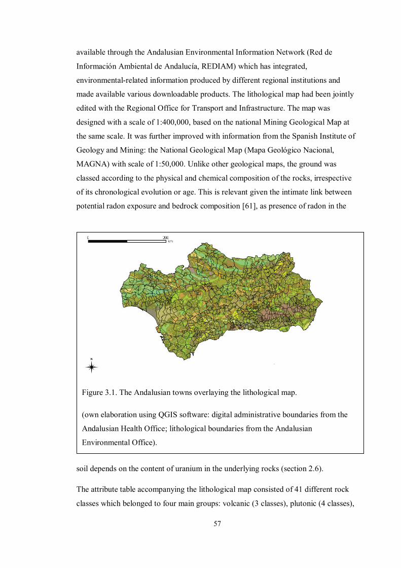
57

available through the Andalusian Environmental Information Network (Red de

Información Ambiental de Andalucía, REDIAM) which has integrated,

environmental-related information produced by different regional institutions and

made available various downloadable products. The lithological map had been jointly

edited with the Regional Office for Transport and Infrastructure. The map was

designed with a scale of 1:400,000, based on the national Mining Geological Map at

the same scale. It was further improved with information from the Spanish Institute of

Geology and Mining: the National Geological Map (Mapa Geológico Nacional,

MAGNA) with scale of 1:50,000. Unlike other geological maps, the ground was

classed according to the physical and chemical composition of the rocks, irrespective

of its chronological evolution or age. This is relevant given the intimate link between

potential radon exposure and bedrock composition [61], as presence of radon in the

soil depends on the content of uranium in the underlying rocks (section 2.6).

The attribute table accompanying the lithological map consisted of 41 different rock

classes which belonged to four main groups: volcanic (3 classes), plutonic (4 classes),

Figure 3.1. The Andalusian towns overlaying the lithological map.

(own elaboration using QGIS software: digital administrative boundaries from the

Andalusian Health Office; lithological boundaries from the Andalusian

Environmental Office).

58

metamorphic (15 classes) and sedimentary (19 classes) [60]. In Spain, radium is

present mainly in some types of rocks such as granite (that belongs in the plutonic

group), clay (which is a sedimentary rock), and shale (metamorphic) [58, 61].

However, other rocks, such as sandstone (sedimentary) and carbonate rocks

(metamorphic) can also be a radium (and hence, radon) source. Therefore,

classification of rocks in the four main lithological groups (volcanic, plutonic,

metamorphic, and sedimentary) where considered appropriate to deriving a surrogate

measure for potential radon-gas exposure. With the aim of estimating the surface that

each lithological group occupied within each municipality, the digitised version of the

lithological map of Andalucía was imported into ArcGIS. All different lithological ID

codes were re-coded to fit into the four main lithological groups and their respective

areas (in square kilometres) were computed using ArcGIS software.

3.3 Mortality data

Data from the Andalusian Mortality Registry were directly provided by the regional

Health Office (Consejería de Salud). The Health Office is the governmental body in

charge of public-health policy development. It is also responsible for supervision of

health-care management and supply [201]. Several other public institutions are also

involved in supplying death-related information to help accomplish all the necessary

registering activities, which leads eventually to electronic mortality records. One of

the collaborating institutions is the Andalusian Statistics Institute (Instituto de

Estadística de Andalucía), which is responsible for the coordination of statistical

activities implemented by attached bodies. The Institute is also in charge of creating,

maintaining and managing regional statistical-databases using available information

from various administrative sources [202]. So, death-related information sources are

comprised of death certificates and death statistical forms (Boletín Estadístico de

Defunción). As required by law, the physician certifying the death provides all the

information included in the former, while they only complete the latter on those

sections related to the causes of death. The rest of this form contains information about

the identity of the deceased, which is provided by relatives or acquaintances. The

municipal Civil Registry where the death takes place, supply additional administrative

data. On a monthly basis, Civil Registries from all 770 municipalities send collected

certificates and statistical forms to each of the eight corresponding provincial branches

of the Statistics Institute [203].

59

The Andalusian Statistics Institute then implements quality-control activities. It

produces electronic records while checking for comprehensiveness and consistency of

information. At a further stage, it sends those electronic files to the Natural Population

Movement Unit (Unidad de Movimiento Natural de la Población). This unit,

comprising staff from both the Health Office and the Statistics Institute, is responsible

for coding all causes of death. The set of criteria used for this task is the International

Classification of Diseases (ICD), as established by the World Health Organization

(WHO) [67]. Information on deaths has been collected electronically from the year

1975 onwards. For that purpose, the ICD-8th revision has been in use to record deaths

that occurred from 1975 to 1979; the ICD-9th revision was used from 1980 until 1998,

while the ICD-10th

The resulting socio-demographic information is eventually passed onto the Andalusian

Mortality Registry, within the Health Office. Available data include: date (day, month

and year) and place of birth (municipality and province); sex, marital status (single,

married, widow, or separated/divorced); occupation, according to twelve main groups

of the National Classification of Occupations (Clasificación Nacional de

Ocupaciones); place of residence (province and municipality (see section

revision was introduced in 1999. Quality-control activities are

systematically implemented for both the socio-demographic and death-cause variables:

data retrieval is accomplished wherever there is some missing information on the

death statistical forms; coding revision and checking of consistency, between the

underlying cause of death and socio-demographic variables are also implemented

[203].

3.2) and

place and date of death registration, which usually (but not always) coincides with

each other. For statistical purposes, place of usual residence (instead of place of death)

is recorded, so that international standards are fulfilled. Even though mortality data are

available for analysis since 1975, year-by-year population data (by age-group, sex and

municipality) are only obtainable since 1981 [204]. Given that population data are

required to estimate the expected number of cases and therefore the SMRs, mortality

data previous to 1981 were discarded for the modelling stage of the work.

Information on deaths, as provided by the Andalusian Health Office, needed data

handling before analysis. Data were provided as a Microsoft Access file, where

anonymised information had been aggregated according to the number of deaths by

municipality, year, sex, and cause. The original wide-code format (19 distinct age-

60

group variables, from ‘0-1’ to ’85 and older’) was converted into a long-code format

(one single age-group variable with 18 values, from ‘0-4’ year olds to ’85 and older’).

By doing so, comparability with age-groups used by available population data (see

section 3.4 below) was made possible. This produced a more than twofold increase in

the number of records, although it gave a ready-to-analyse file. Epi Info software

versions 3.5.1 (launched in 2008) to 3.5.3 [205] were used to handle data import and

conversion given its relational-database capabilities and Microsoft Access

compatibility and the previous experience of the author. Since then, a new version of

Epi Info has been released [206]. Many different scripts were also written (using Epi

Info and R), or adapted (using WinBUGS and R), to support quality of data-

acquisition and analysis. In this way, any disagreement between original and derived

files was double-checked by reviewing and amending, where needed, the

corresponding script. Further data-handling was required, due to changes in

administrative boundaries throughout the study period. The Andalusian Statistics

Institute provides online information about aggregation and segregation of

municipalities [204]. In accordance with that information, some codes had to be

recoded so that they fitted the boundaries later used for the mapping process (see

section 3.2). Recoding affected 11 out of 770 (or 1%) geographical codes.

After that, cases and populations were aggregated by municipality for each year,

death-cause, age-group, and sex. To reach this stage, I wrote (specifically for this

purpose) several Epi Info scripts. They allowed addition of variables that labeled

codes and, therefore, made analysis output easier to interpret and less prone to error.

That was the case for variables such as death-cause and sex. Another crucial step, to

make sure that population data were accurate, was to produce zero-count records (for

the variable number of cases) where no deaths had occurred. These zero-count records,

represented as missing values in the original 19 age-variables, were unavoidably lost

while adding the number of cases by age. Taking advantage of Epi Info relational-

database capabilities, the case-file was linked to an aggregate population file. This

dataset only shared some variables with the former (municipality, age-group and sex)

while the case-file also contained data on death-cause and year. To prevent manually

repeating the same task, and reducing the risk of error, I wrote new specific scripts to

be run within Epi Info. Missing values were replaced with due codes: death-cause,

61

year of reference or zero-counts. As a consequence, computability of both the expected

number of cases and SMRs figures (see 4.2.1 below) were assured.

All data preparation eventually produced a first file ready for initial descriptive-

analyses of mortality. Only 759 different municipal codes were left, after the recoding

process. Given that Epi Info allows for files to be exported to (and imported from)

different formats, this capability was used throughout the process. It was not only

useful for data-handling, but also helped in the transition to data modelling (especially

where exporting data to R software). Mortality data were directly read into Epi Info

from Microsoft Access files, while population data (see 3.4 below) were imported from

Microsoft Excel files.

3.4 Population and socio-economic data

The Andalusian Statistics Institute (see section 3.1 above) has published online

population-data at the municipal level [204]. Three different data sources are

available: decennial censuses, yearly Municipal Register of Inhabitants (Padrón

Municipal de Habitantes) and year-by-year inter-census population estimates.

Censuses involve large-scale operations at the national level and are paramount for

civil services to plan, manage, implement and follow-up public policies [207]. Both

the national and regional governments have authority on statistics affairs at their

respective scales. Therefore, a collaborative agreement exists between the Andalusian

Statistics Institute and its national counterpart, the Spanish National Statistics Institute

(Instituto Nacional de Estadística, INE,), to coordinate efforts for censuses production

[207]. There are three different types of censuses that record data about resident

population, dwellings, and buildings and premises, respectively. To collect

information on both population and dwellings, four different questionnaires are used

which have been devised to be self-administered by the interviewees themselves.

Nevertheless, concerned people can be also assisted by civil servants if required.

One of these questionnaires (hoja padronal) includes data on individual identification

variables collected from municipal registries. It is intended for the interviewee to

review it and amend it where needed. These variables include place of residence

(province and municipality), date of birth, sex, place of birth (in case of foreigners,

just country of origin) and nationality. A second questionnaire is the home one, which

collects information on marital status, achieved level of studies and type of studies.

62

Occupational status classified people as either in the labour force (employed or

unemployed) or economically inactive.

Another source of population data is The Municipal Register of Inhabitants, which

constitutes the official administrative record that proves place of residence [208].

These data bases are recorded and maintained by every city council across the country

and collect information from all population centres. Although intended for

administrative purposes, as determining financial quotas and legislative representation,

they are also useful for statistical applications. Thus, Municipal Registers (like

censuses) supply information about population counts and its demographical structure,

including age and sex [209]. Both the Andalusian and the National Statistics Institute

provide online access to the Municipal Register of Inhabitants. The National Statistics

Institute server hosts much of the information as PC-axis files. This free-software

format has been developed by Statistics Sweden and is used by many statistical offices

around the world. It is a convenient tool for data tabulation, which also allows for files

to be exported using different formats [210, 211]. In contrast, the regional website

provides on-screen spreadsheet views that can only be copied and pasted, which would

make data retrieval cumbersome [212]. Therefore, PC-Axis software (2007 version)

was also downloaded from the National Statistics Institute to read and export data

from the Municipal Register of Inhabitants. Inter-census population estimates (by

municipality, sex and five-year age-groups), were available for the period 1981-2001.

A single PC-Axis file was available through the Andalusian Statistics Institute

website. It comprised population data by municipality age-group and year, which

included both the study period (1986-1995) and the period used to provide prior

probabilities to implement a sensitivity analysis, concerning the clustering and

heterogeneity components (1981-1985). This file was exported to dBASE format and

then read from Epi Info to combine all 18 age-variables into a single one, using a

purpose-written script.

Socio-economic information was drawn from the census. Data from the 1991 census is

available online both through the Andalusian and the National Statistics Institute

websites [212, 213]. Therefore, population census data needed to compute area-level

socio-economic deprivation were downloaded from the National Statistics Institute

website as PC-axis files. Three different files were obtained on the number of people,

by municipality, who were illiterate, unemployed and doing manual jobs. As those

63

files consisted of information concerning all Spanish municipalities, they were

exported to exploit Epi Info relational-database capabilities. This made it possible to

select only Andalusian municipalities, more efficiently than through a highlight-and-

select process available within PC-Axis. A previous step though, was to export these

files to Microsoft Excel format. The aim was to exclude some values of no use and

make some calculations prior to computing the deprivation scores.

The original PC-Axis file related to literacy level had three fields: municipality, sex

and literacy level. The files on employment level and job description had the first two

fields (municipality and sex) in common. The municipality field had 8,127 unique

numerical codes followed by their literal names, as one single character-string within

the same field; sex had values for both sexes and the total number of people; the

literacy level was classified according to thirteen different classes (from illiterate to

doctorate, plus several subtotals and a grand-total value). Since only three of these

values on literacy level were needed, the rest were not exported to Microsoft Excel.

Then, only the total-population count, and the number of people who were illiterate

(not able to read or write) or had no studies degree were exported to Excel format. Sex

counts were not exported, as the area-level deprivation index did not intend to address

sex differences in populations. Illiteracy has been previously defined as the number of

people (10 years or older) who were illiterate or had no studies [28, 155]; it was

computed by the author (using Microsoft Excel) as the percentage out of the total (10

years or older) population.

The employment status had been classified in the original PC-Axis file using eleven

different categories. Both the economically-active (16 to 64 year olds) and inactive (all

others) populations had been included by the National Statistics Institute. The former

group had been divided in three different classes: employed, unemployed looking for

their first job, unemployed who had worked before. The latter had been classified in

four groups: retired, students, doing housework, and others. Additional subtotals and

grand-total counts completed the original variable about employment level. The

unemployment component has been previously defined as the number of unemployed

people within the economically-active population [28, 155]. It was computed as the

percentage out of the total economically-active population. The Manual workers group

is defined as people belonging to any of the following five (out of twenty) different

64

classes: those specialised in building construction, mines and metallurgic industries,

any other industries, machinery and facilities, and non-skilled workers [155].

Once all deprivation components (percentages of illiteracy, unemployment, and

manual workers) were computed, a Microsoft Excel file was created that also included

the municipality codes. That file was then imported into Epi Info to select only those

records which municipality code belongs to Andalucía (see section 3.2). After that, the

file was exported to R software (as a dBASE file) to implement a Principal

Component Analysis (PCA) and subsequently produce an area-level (by municipality)

deprivation score. This final deprivation score (computed for the 759 municipalities)

had a median value of 0.01 and standard deviation 1.18. The minimum and maximum

values were -3.46 and 3.38, respectively. The interquartile range was 1.58. As a

measure of material deprivation, the higher the score, the more deprived an area is.

65

Chapter 4. Methods

4.1 Overview

This section will describe the health outcomes that were analysed (mortality due to

lung cancer, larynx cancer and COPD) and how the magnitudes of their effects were

estimated and subsequently modelled and mapped. Details will be given on how

mortality estimates were computed for both men and women. Firstly, the use of

internal, indirect, standardisation to compute the SMRs for all three mortality causes

will be presented. Secondly, the modelling process will be described in detail.

Two different models were used to explain geographical heterogeneity in the mortality

distribution. Firstly, a Structural Equation Model (SEM) [195, 196] was fitted to

confirm that rock composition (as a surrogate measure for potential content of radon-

gas in the soil) explained spatial heterogeneity in a lithology score. This lithology

score, in turn, was produced from a Conditional Autoregressive (CAR) model as it

was hypothesised to be spatially auto-correlated. That is to say, lithology of

neighbouring areas was expected to be more similar to each other than to

geographically-distant areas. Secondly, a BYM model was used that split the residual

(not explained by the model) variance into two different components: spatially auto-

correlated heterogeneity (CH, or clustering) and uncorrelated heterogeneity (UH, or

random heterogeneity). In both cases (the SEM and BYM models) adjustment for

socio-economic status (SES) at the area-level was implemented using a deprivation

score. This deprivation score was computed by means of Principal Component

Analysis (PCA) that made use of the percentage of illiterate and unemployed people,

as well as the percentage of manual workers, by municipality.

Lastly, mapping of SMRs, and RRs obtained from the BYM model will be presented

for lung-cancer mortality, separately for both men and women. Individual RR maps

will be shown for each of the model components so that they are visually appraised.

Thus, maps of RR due to lithology, deprivation and the residual variance (both

clustering and heterogeneity) will be presented. Also, exceedance probabilities maps

(of an RR being greater, or less, than 1) were produced to convey the likelihood that

there is an excess, or lack, of risk of mortality for lung cancer, at some specific areas.

66

4.2 Health outcomes estimates

4.2.1 Estimates of the expected number of cases

Any mortality (or morbidity) frequency measure used to compare different populations

must consider structural differences that may exist among them. Then, age and sex, as

well as social class are considered to be common potential confounders to be adjusted

for. This consideration is based on: firstly, these covariates may be simultaneously

related to both the outcome and the exposure of interest; secondly, these relationships

may be independent of each other; thirdly, the populations may differ in the

distribution of the covariates. When these circumstances are present, a confounding

effect may bias the statistical association between the exposure of interest and the

outcome. As a result, any association (e.g. as measured by means of the relative risk)

may be either overestimated or underestimated. When an exposure-outcome

relationship is confounded, a true statistical association may not be detected; and the

reverse, a finding of a spurious statistical association, may also happen. To address a

potential confounding effect in the analysis stage of observational studies, different

solutions can be implemented. Three different techniques have been used in this

thesis: standardisation, stratification, and multivariable regression analysis.

Standardisation was used to take account of differences in the age structure of the

populations under comparison. Stratification was applied so that data for males and

females were analysed separately. Multivariable regression analysis adjusted for area-

level deprivation while estimating the effect of lithology, on mortality.

To accomplishing age-standardisation, the indirect, internal, method was used; it

started with rates coming from age-groups of an internal population (the whole

Andalusian population) which were then multiplied by the within-strata study-

population sizes corresponding to each geographical area [214, 215]. In this way, the

expected numbers of cases were estimated and, then, summed across strata (age

groups). Then, the ratio of observed to expected numbers was computed to derive a

frequency measure. This ratio is the SMR. In this scenario (a small number of cases

arising from a relatively large population), the observed number of cases is considered

to be Poisson distributed. Under this assumption (which must be checked) the SMR is

the Maximum Likelihood Estimate (MLE) of the RR [43, 63, 73].

67

Another important step in the SMR computation process is to choose the population

providing the rates [43]. Internal standardisation was used where the rates came from

the addition of every single study population, as a whole. An iterative computational

method devised by Mantel and Stark and subsequently simplified by Breslow and Day

has been used in the past for rate standardisation [70, 71]. These methods are based on

the assumption of a multiplicative model for the distribution of the observed number

of cases. Consequently similar results can be achieved by fitting a Poisson regression

model on the log scale [43, 47, 90]. Nevertheless, modelling of the SMRs by basic

Poisson regression has some limitations. One of the restrictions of the Poisson model

is that the variance and the mean are assumed to be equal. This assumption is, in

practice, difficult to maintain and overdispersion (that is, the variance being larger

than the mean) may occur. Overdispersion can arise due to one or more of the

following: spatial autocorrelation, an excess of zero-event values (such as in a rare-

disease situation), or just random heterogeneity [44, 90, 216, 217]. Where a Poisson

model does not fit the data, it underestimates the standard error of the point estimates

for the explanatory variables.

As an alternative a Negative-Binomial model, which allows for overdispersion, might

be fitted, instead. The Negative-Binomial distribution would give the same point

estimates, but larger standard errors, and hence, wider confidence intervals. Another

difficulty that both the Poisson and Negative-Binomial models can encounter is when

fitting data where an excess of zero-values (sparseness) is present; this may be the case

where rare diseases are analysed. In these instances, a Zero Inflated Poisson (ZIP), or

Zero Inflated Negative Binomial (ZINB) model can be useful alternatives. However,

neither ZIP models, nor ZINB models, take spatial auto-correlation into consideration.

Nevertheless, both ZIP and ZINB models can be further extended to accommodate

complex hierarchical structures that account for both, spatial auto-correlation

(clustering), and unstructured (heterogeneity) effects.

Therefore, to account for the potential confounding due to differences in the age-

structure of the populations being analysed, age-adjusted SMRs estimates were

calculated for both men and women in every Andalusian municipality. Estimates were

calculated for a total of 759 municipalities, for the periods 1981-1985 and 1986-1995.

Internal, indirect standardization [51, 62, p. 312-5] was used that obtained the rates

from the whole study population. Subsequently, the rates and the corresponding study

68

populations were used to estimate the expected number of cases. These figures were

applied, in turn, to model the SMRs via Bayesian regression analysis (see 4.2.2). The

SMRs were computed for all three distinct mortality causes: lung cancer, larynx

cancer, and COPD.

To obtain age-and-sex adjusted rates, the glm (generalised linear models) function

(within R stats-library [218]) was used to fit separate Poisson regression models to the

data concerning mortality due to lung cancer, larynx cancer and COPD, respectively.

The outcome of interest was the observed number of cases and the variable population

was specified as an offset. The starting point was a saturated model, where the

predictor variables ‘age-group’, ‘sex’ and the interaction ‘age-group by sex’ were

included. The Akaike Information Criterion (AIC), or penalised log-likelihood, guided

model fitting [77, p.353-4]. The AIC is a derivation of a likelihood ratio test [215, p.

309-10] which in addition takes into consideration (penalises) complexity of the

model, according to the number of parameters included. The automated stepAIC

function was used: it drops one parameter at a time and prints the value of AIC for

each model. The model with the minimum-significant AIC was chosen. The saturated

model (age-group + sex + [age-group*sex]), remained as the minimum adequate

model.

The subscript utility, available within the R software, was used to write a script that

recorded the estimated rates of age-groups for each sex. This utility allows for access

and manipulation of any elements stored within R objects (vectors, matrices, arrays,

data frames and lists) [219]. The output produced after fitting a Poisson regression

model (by means of the glm function) produces a list object or, more precisely, a list

of lists. One of its elements contains the regression coefficients estimated by the

model. These coefficients can be extracted as a group, using the ‘coef’ function

available in the R stat-library [218]. Alternatively, the regression coefficients can be

individually referred to by means of the subscripting utility, which allows for the

manipulation of its values. So, the regression coefficients resulting from Poisson

regression analysis were accessed and the estimated rates were computed in the

original, multiplicative, scale: that is, as the antilog of the corresponding linear

combination of parameters (age-group, sex and the interaction between them, plus the

intercept). The resulting variable, the estimated rates, was then merged with the file

containing the observed number of cases by municipality. To accomplish this task,

69

both files were linked by common fields (age group and sex) by means of the same

script. Additional information contained in the final file included yearly population

size, as obtained during data collection (see 3.4).

The estimated rates previously obtained allowed the computation of the expected

number of cases and, consequently, of the SMRs. Firstly, the rates were multiplied by

the population size to calculate the expected number of cases. Figures were obtained

for age group, sex and yearly strata within every municipality. The data were

aggregated by municipality where each one had a total number of observed and

expected cases, per year. All this computation was accomplished using Epi Info

software, where the summarise function (within the Analyse Data module) allowed for

data aggregation. The next step, computing the SMRs, required further modelling

implementation.

Although SMR calculation (as the ratio of observed over the expected number of

cases) is apparently straightforward, two different issues were to be addressed:

computational difficulties and spatial auto-correlation. When SMRs are calculated at

the small area level, instability of the ratios (due to small expected number of cases) is

likely to be encountered, leading to imprecise estimates. This can happen in the

presence of either rare health events, and/or very small study populations. The second

issue, spatial auto-correlation, concerns the lack of independence of observations.

Both difficulties were addressed by modelling the SMRs using WinBUGS software,

assuming that the observed number of cases followed a Poisson distribution. The

previously estimated expected number of cases, instead of the populations was used as

an offset [220]. Age-group and sex (as well as the interaction between both variables)

were adjusted for as in the previous model and for the same periods of time (1981-

1985 and 1986-1995). To allow for spatial auto-correlation, the BYM model was used;

it partitions the residual variance into two different components: correlated

heterogeneity (CH, or clustering) and uncorrelated heterogeneity (UH, or random

heterogeneity) [63, p. 123-7, 221, p. 84-92, 119]. The clustering component arises

from a Conditional Autoregressive (CAR) model; in the BYM model, the log disease-

rate of a particular area is a function of both, explanatory variables, and potential

confounders. The local average of disease rate in neighbouring areas partially pools

(or smoothes) the original rates towards a local mean-value [222]. For the present

analysis a queen-style adjacency weight-matrix was defined using the ‘nb2WB’ R-

70

software function, implemented within the R ‘spdep’ library [223]. This neighbouring

definition (which borrows its name from chess moves) considers polygons to be

neighbours if they share either a single boundary or vertex (section 4.2.2 ). The second

component of the residual variance in the above-mentioned BYM model is the

spatially-uncorrelated (or random) heterogeneity. This component was modelled as a

normal distribution.

4.2.2 Modelling of Standardised Mortality Ratios

Observations arising from the same or close geographical areas tend to be similar to

each other, while observations at locations which are far apart from each other tend to

be dissimilar. These kinds of processes give rise to observations that are said to be

clustered (or pseudo-replicated); that is to say, they are not independent from each

other. In this situation, usual statistical estimates would produce too-narrow Credible

Intervals (CIs), so that the effect of the explanatory variable of interest would be

imprecisely estimated. As a further downside, this analytical method would prevent

from gaining knowledge about any residual variability that is spatially correlated.

Consequently, a specific statistical approach is needed to address spatial

autocorrelation. One simple alternative could be to summarise information for each

individual area (no-pooling analysis). The drawback of such an approach is the

potential instability of the SMRs [63 p. 4-5]. Extreme values would be estimated for

areas with small population size and, hence, low number of expected cases. These

extreme estimates would have over-estimated standard errors. To overcome this

difficulty, individual-area estimates can be weighted (partial-pooling analysis,

shrinking, or smoothing) according to their relative variance, as compared to an

average variance. Estimates based on smaller denominators would express a value

close to the average; conversely, estimates based on larger denominators would show

a magnitude closer to the individual (un-weighted) area-value. In this way, emphasis is

laid on the most reliable estimates. To weight the estimated SMRs, different

approaches can be made to decide about the kind of smoother to use; this, in turn, is

closely related to the computation of the adjacency matrix, which is a crucial element

when Conditional Autoregressive (CAR) distributions are used to implement

hierarchical models [224].

71

The adjacency matrix is actually comprised of three different matrices that contain

related pieces of information. Two of them contain the polygon identification and the

number of its adjacencies (neighbouring polygons) which provide the neighbour

definition adopted by the researcher. A third one gives the weights assigned to each

polygon, which will contribute to the smoothing of outcome estimates. Even though

GeoBUGS (version 1.2) can easily generate the adjacency matrix, a potential flaw

exists: this software does not check that any particular area is not specified as its own

neighbour. For this reason, R (instead of WinBUGS) was chosen to compute the

adjacency matrix. The spdep (spatial dependence) library [223] has different functions

to create neighbours lists from polygon data frames. So, the poly2nb function was used

to create an R neighbour list from the imported municipal shapefile. Then, the nb2WB

function exported that information into WinBUGS, 3-dimensional array, format.

Differently to WinBUGS, R allowed for checking that no area was declared as a

neighbour of itself. The function nb2mat produced a binary weights matrix, where

neighbour relationships were coded as 1 and lack of vicinity as 0. It was then

straightforward to use the diag function to check values from the matrix main

diagonal: all of them were 0, as the leading diagonal represented municipality self-

matches.

Different generic terms are in use to refer to models devised to allow for clustered

observations: Multilevel, mixed models, cross-sectional time series, random effects, as

well as hierarchical-models, which is the term used henceforth in this thesis. Among

the vast array of hierarchical-models applicable to this study, many of them assume

that the observed number of cases follows a Poisson distribution. In these models, the

mean value (for each area and stratum) is the product of the estimated rate times the

expected number of cases. Nevertheless, this assumption has to be checked given that,

in a very rare-disease situation, it might not be valid. In these cases, sparseness of data

may lead to an excess of zero values, which would make it inappropriate to model the

data as if they followed a Poisson distribution. To overcome this difficulty a Zero

Inflated Poisson (ZIP) model can be fitted (section 4.2.1).

Two main strands of computational techniques can be followed to fit spatial models:

frequentist and Bayesian analytical approaches. The former has been the standard

statistical approach to data analysis for a long time. Nevertheless, Bayesian statistics

have gained widespread use in the last few years. This is mainly due to the availability

72

of fast hardware, modern computational techniques, and software. Current hardware

helps taking advantage of Bayesian strengths while managing computational demands;

computing techniques based on simulation, like Markov Chain Monte Carlo methods

(MCMC), assist in modelling complexities. Practical feasibility of Bayesian analysis

has influenced its widespread use as the benefits now outweigh previous difficulties.

One of the advantages of using a Bayesian approach is related to the overall

performance of Bayesian estimates. From the frequentist point of view, the best

estimator (the Maximum Likelihood Estimate [MLE]) is the minimum-variance,

unbiased estimator. Performance is then measured by the Mean Squared Error (MSE),

which is a linear combination of both, variance, and bias. Even when the frequentist

criterion is applied to assess Bayesian estimates, these usually outperform the

frequentist ones. This happens as the former can be much more precise than the latter.

This causes the MSE to be lower for Bayesian estimates in many instances, especially

with small simple sizes.

Some other advantages of Bayesian estimation are related to the integration of

information, as well as interpretability. Frequentist inferences are based on the MLE;

this is the most likely value that the sample statistic would represent, assuming an

underlying probability model. This statistic would estimate the unknown, but fixed,

parameter with certain error (which determines the confidence interval width). All of it

provided the, unrealistic, scenario that the experiment under consideration was

repeated an indefinite number of times. Therefore, both the point estimate and the

confidence interval are not referred to the sample actually obtained; it is a theoretical

range of values that would be obtained in the long-run. In contrast, the Bayesian

approach brings together two different sources of information to produce inferences:

information coming from the actual data under the assumed probability model (the

likelihood), and previous beliefs (the prior probability). These two give the inference

(the posterior probability). Its foundation is based on the Bayes’ rule that relates to

conditional probabilities. Using Bayes’ rule, it is possible to estimate the probability of

any conditional event, if the probability of the related one is known. This foundation

makes the inferential process divert greatly from frequentist methods.

Consequently, a direct probability statement can be made about the parameters of

interest, as they are considered to be random variables. And the same direct

interpretation applies to estimates of error (credible intervals). A further advantage of

73

Bayesian analysis is that inference is not limited to point estimates (and error

measurement); the posterior probability gives the whole probability distribution of the

estimated parameter. It is also important to note that even when numerical results

obtained by both methods are similar, interpretative differences still remain. Similar

results may be obtained by both methods as they all use information provided by the

likelihood, in the inferential process. In the Bayesian approach, though, the likelihood

is weighted by the prior probability; therefore, a low weight (vague prior) would not

modify the likelihood to a great extent.

Notwithstanding this circumstantial agreement in the results, some more advantages

can still favour the use of Bayesian methods, as these incorporate prior beliefs into the

modelling stage and can take advantage of simulation (random number generation).

Use of the prior probabilities allows for inclusion of uncertainty about the parameters,

which are now considered to be random variables. This is useful as new knowledge is

an ever cumulative experience. It is also feasible given that researchers are usually

aware of some kind of previous information. As data quality is always essential,

choice of prior information is a key element, as it influences (together with the

likelihood) the posterior estimates. This is the reason why a sensitivity analysis is

frequently advocated to decide on the best prior to use.

Simulation is another asset that Bayesian analysis can use. Inferences based on

simulation rely on random number generation, instead of point estimates and standard

errors, to summarise results. As a result, an exhaustive description of inferences is

obtained in the form of a probability density function. Simulation is considered to be

the most reliable method to address inferential uncertainty and is well suited for very

small sample size situations. In these cases, frequentist methods rely on the Central

Limit Theorem to assume that the normal distribution assumption is valid. Simulation,

instead, allows for an increment of sample size nearly at will and hence, helps to

reduce uncertainty. It also accommodates complicated models, which makes it

convenient to fit hierarchical structures, irrespective of the assumed probability model.

Notwithstanding the advantages that simulation entails, Bayesian analysis can also be

tackled from a different perspective.

Bayesian models can be broadly categorised as Empirical Based (EB) or Full Bayes

(FB) methods. The former approximate the posterior distribution and estimate

74

hyperprior values from the data; conversely, the latter draw samples from the exact

posterior distribution and estimate hyperpriors from different data sources. FB

methods use a range of algorithms within the common family known as Markov Chain

Monte-Carlo (MCMC) methods. By using MCMC, FB methods overcome some

difficulties that EB methods may encounter. EB methods are based on numerical

integration to calculate the posterior distribution, which may be difficult where a high

number of parameters are to model. In these situations, only an approximation to the

posterior may be achieved. As an alternative to calculating the posterior distribution,

FB methods draw a random sample from the posterior. An immediate advantage of

this method is that the sample size can be increased to reach the desired precision.

Also, given that FB computation is not a major issue nowadays, a vast array of models

with varying complexity can be fitted.

Several hierarchical models have been proposed for the spatiotemporal analysis of

epidemiological data. The BYM model is a FB method that allows for spatial auto-

correlation [62, p. 321-32, 63, p.123-7, 92, 225, 226]. A hierarchical model is

assumed, in which a random effect variance-component is set as a mixture of

correlated (spatially structured) and uncorrelated heterogeneity. The spatially-

structured variance is then given a prior distribution under the Conditional

Autoregressive (CAR) assumption which shrinks SMRs according to a local mean

depending on neighbouring estimates [62, p. 282-7]. The car.normal distribution

function (available in WinBUGS) was used to model the prior probability for the

spatially-structured component of the variance [63, p. 70-1, 123-7]. Fitting this model

required information about the adjacency matrix which defines neighbouring of spatial

polygons (see 3.2). This information was supplied and exported as data, from R into

WinBUGS. A binary weighting list was also required by the model, which assigns the

value 1 in case a polygon is a neighbour of some specified area, and 0 otherwise. This

is the simplest way to build an adjacency matrix and the accepted standard when no

other assumptions are being considered; that is, just the mere existence of

neighbouring areas, with no additional knowledge or hypotheses concerning

geographical links.

75

4.3 Software description and analysis implementation

To be able to model the SMRs by means of the BYM model, different pieces of

software were used: R [218] and WinBUGS [227] were especially relevant. Both R

and WinBUGS are free software, readily available on the internet. R is very well

suited for data analysis, statistical modelling and graphical representation, as well as

data manipulation (see 4.2.2). One of its main advantages is the availability of many

different packages that can be installed to tailor specific needs. The spatial

epidemiology field is not an exception and different packages have been developed to

assist in different steps: from data import through data manipulation, analysis and

export [50]. Especially relevant is the ability of R to import/export data with different

formats. This helped in data manipulation and analysis, as files could be transferred

from and to different specialist software, like Epi Info, WinBUGS and GeoBUGS.

WinBUGS is also free software, devised for complex data analysis using a Bayesian

approach through MCMC methods (specifically the Gibbs sampling algorithm). The

BUGS project has become open-source [228] and future developments will be only

made for this version. Nevertheless WinBUGS v1.4.3, which is a stable version, will

remain available. GeoBUGS is an add-on module to WinBUGS (and OpenBUGS) that

allows for spatial representation of data. It is particularly convenient for immediate

mapping of data after they are modelled using WinBUGS. GeoBUGS can also assist in

creating the adjacency matrix needed to fit Conditional Autoregressive (CAR) models.

Nevertheless, it does not check that each polygon is not included as its own neighbour;

for this reason R was used instead, at this step (see 3.2). Different R packages were

used to accomplish these tasks: ‘maptools’ [229] and ‘spdep’ [223] were useful to

address boundary data (see 3.2) and the spatial information related to the adjacency

matrix.

Convergence is at heart of MCMC methods. All simulated chains are expected to

reach a common equilibrium state, beyond which they would keep giving the same

estimation. This estimation (the posterior distribution) would be an accurate

representation of the target distribution, irrespective of the initial starting point for

each chain. The BGR statistic is a convergence diagnostic tool that can be used when

more than one Markov chain is run. It is calculated as the ratio of the variability of

pooled chains over the average variability of all chains. At an early stage, the BGR

76

statistic ( R̂ tends to be greater than 1. As simulated chains reach a state of

equilibrium, the statistic becomes closer to 1. Gelman suggests a value of R̂ ≤ 1.1 to

consider that convergence has been approached, or at least R̂ ≤ 1.5 for some

parameters, if the process is slow. This latter value is the one Spiegelhalter suggests be

used. It may be also interesting to analyse convergence using WinBUGS to map

results in GeoBUGS, immediately after that.

WinBUGS can apply a number of diagnostic-tools. So, autocorrelation histograms

help in deciding about the thinning interval, the burn-in period, and the total number

of iterations to run. Given that the initial estimates of any MCMC chain tend to be

highly auto-correlated, it is standard procedure to discard part of it; this is the burn-in

period, which can be incremented to try sampling from the posterior distribution at its

equilibrium state. The autocorrelation graph also provides details about the lag beyond

which autocorrelation becomes negligible. This information is used to reduce the

number of iterations kept, which saves computer memory. This is quite relevant as

WinBUGS, like R, stores all output analysis in the computer random-access memory

(RAM). Consequently, too much output-data can cause the software to crash by

exhausting all available memory.

There are at least two circumstances where computer-memory exhaustion may be

encountered: first, if too many parameters are monitored at the same time; secondly, if

too many iterations are run. The former may arise where several estimates for many

different areas (such as the 759 different municipalities, in this study) are monitored.

The latter may happen where precision of estimates needs enhancing, by running long

chains. To address the first issue, parameter monitoring should proceed gradually. To

counteract the second one, a thinning interval can be used; in this way, only one in

several iterations is actually kept (e.g. 1 in 10, if thinning is set to 10). After the

software has finished running a first set of foreseen iterations, convergence has to be

checked.

When the MCMC process consists of more than one chain, WinBUGS allows for

graphing of BGR statistic against the number of iterations. The graph represents

values of BGR in three different lines: The green one shows the variability (as 80%

width intervals) of posterior estimates of pooled chains. The blue one corresponds

with the average within-chain variability. Finally, the red one is the ratio of between-

BGP

Typewritten Text

BGP

Typewritten Text

)

BGP

Typewritten Text

77

chain to within-chain variability ( R̂ ). As all the chains approach the equilibrium state,

they become similar to each other. Therefore, the BGR statistic is close to 1 and both,

the lines representing variance between chains, and within chains, tend to stabilise.

Other graphs are also available to check convergence. So, trace plots represent

sampled estimates against the iteration number. Where chains are approaching

convergence, they tend to mix with each other adopting the ‘fat hairy caterpillar’

shape. It is important to allow that the chains start from different points and afterwards

assess convergence towards a common distribution.

To run different chains, initial values have to be provided for every stochastic node

(random parameter). In the model that was fitted, initial values were set for elements

that composed the residual variance, that is, clustering and heterogeneity. Different

possibilities exist to decide on the initial values for each chain. Thus, WinBUGS can

generate initial values. However, it has been reported that this method may cause the

software to crash. Therefore, random values were generated in R, and passed as data

into WinBUGS. An important decision concerning initial values has to do with the

underlying distribution from which the values are generated. This is especially

relevant where estimates concern parameters of prior distributions (hyperparameters).

Consequently, it is worth considering a sensitivity analysis where alternative initial

values, arising from different distributions, are used each time. Some researchers

especially advocate not using the inverse-gamma vague prior to estimate variance

parameters. The rationale behind this recommendation is that this distribution, which

is ‘L’ shape, strongly constrains the posterior. As a result, the posterior distribution

becomes very sensitive to the chosen parameters. When vague priors are used, some

researchers suggest generating values from normal distributions for all stochastic

nodes, with the exception of variance parameters, which are constrained to be positive,

in which case the uniform distribution would be used, instead of the inverse-gamma

one. Yet another possibility is to take advantage of previous knowledge from actual

data; this information can be used, therefore, as the prior probability. This seems most

appropriate, as FBM are intended to integrate past knowledge into current data.

According to this, the BYM model was fitted to mortality data from 1981-1985 to

generate prior information, about hyperparameters; this hyperprior values were used,

afterwards, to fit data from the period 1986-1995.

78

4.4 Ecological analysis

4.4.1 Socio-economic Status

Socio-economic Status (SES) is a highly relevant covariate to take into consideration

both in individual-level studies and ecological research (see 2.4). It has been

extensively reported as a confounder in many epidemiological associations between

different exposures, and health-related events. Furthermore, SES has been also

considered a relevant explanatory contextual variable by itself. It was accounted for

through an area-level deprivation index. This index was based on percentages (by

municipality) of: unemployed and illiterate people, as well as manual workers.

Principal Component Analysis (PCA) was used to derive this area-level deprivation

score.

Subsequently, unmeasured variables with potential spatial dependencies (also known

as contextual effects) were taken into consideration. To adjust for these unmeasured,

spatially auto-correlated effects, general clustering of mortality rates was taken into

consideration. To this end, a BYM model was fitted to lung cancer mortality data in

both men and women. This way, the residual (not explained by the model) variance

was split into two different components: clustering (or spatially correlated variability)

and heterogeneity (or non-spatially correlated variability). The BYM model took also

account of both area-level deprivation score from PCA analysis, and the lithological

risk score derived from the SEM.

4.4.2 Potential radon-gas exposure

Spatial heterogeneity in rock composition (lithology) was hypothesised to be

associated with geographic disparities in mortality rates due to lung cancer. This

hypothesis was based upon two grounds: firstly, the correlation between lithology and

content of radon-gas in the soil, according to previous studies; secondly, the reported

effect of radon-gas exposure, which is considered to be a main risk factor in lung

cancer development. The spatial dependence of mortality on lithology was also

evaluated for two additional outcomes: chronic obstructive pulmonary disease

(COPD) and larynx cancer. The reason for extending the analysis to these additional

outcomes was based on previous knowledge showing that while tobacco smoking was

a major risk factor for all the three conditions, radon-gas exposure has only been

associated with lung cancer incidence.

79

Structural Equation Modelling (SEM) was used to assess the value of lithology in

explaining geographical differences in mortality rates. The structural part of the SEM

took account of a lithological risk score derived from a spatial Conditional

Autoregressive (CAR) distribution. The measurement part of the SEM assessed the

explanatory value of lithology on the lithological risk score. The SEM was fitted to

mortality data due to each one of these three distinct causes: lung cancer, COPD and

larynx cancer.

4.5 Disease Mapping

GeoBUGS software v 1.2 (an add-on to WinBUGS) was used to map raw and

smoothed SMRs, the latter ones being labelled as RR to differentiate between them

(sections 4.2.1 and 4.2.2). Also, statistically significant RRs were mapped as the

probability of an RR being greater than 1. Given the small range of posterior RR

estimates beyond 1, under the BYM model, no other threshold references were

considered. Both spatially-structured and uncorrelated heterogeneity were mapped,

where a relevant pattern was important to highlight. For this purpose, regional digital-

boundaries in shapefile format were imported into R; afterwards, the file was exported

into S plus format to be read from GeoBUGS (see section 3.2). Once the map was read

into GeoBUGS, mapping was accomplished following the modelling stage

implemented using WinBUGS. After modelling of the SMRs was completed, some

other issues had still to be considered; among these, which estimate components were

relevant to be mapped and how to represent them.

It is useful to produce maps that convey different sorts of information: thus, raw

(SMRs) and smoothed (RR) maps, as well as individual RR regression components.

By comparing raw and smoothed maps, the degree of shrinking (rendered during the

modelling stage) can be conveyed graphically. This is relevant to be aware of over-

smoothing that would hide the underlying risk variation [230]. Mapping of individual

regression components, on the other hand, can show interesting graphical information

generated through the modelling stage [63]. This is equivalent to partitioning the RR

into estimates of risk that originate from different sources. This is accomplished by

taking the antilog of the corresponding regression coefficients, which can be

programmed using WinBUGS code. In this way, the geographical heterogeneity due to

80

these different sources is highlighted. So, variability in the RR explained by a variable

(such as SES, or lithology) can be mapped.

Especially interesting is mapping of the residual RR. This helps to have a feeling of

the overall goodness-of-fit of the model, which has to be also formally tested (see

4.2.2). This component contains the estimate of the variability not captured by the

explanatory variables (and covariates) allowed for in the model. Under the BYM

model, the residual RR is calculated as the antilog of the intercept plus both, the

clustering and uncorrelated components (see 4.2.2). The last two components can be

also calculated and mapped independently from each other. Mapping of these

components in isolation allows for a graphical representation of where the residual RR

is mostly laid. So, although different diseases can naturally arise in clusters, spatially-

structured variability may also be due to unspecified area-level explanatory variables;

among these, environmental risks or contextual (area level) effects may be potential

explanatory variables for this residual RR. The uncorrelated heterogeneity, on the

contrary, contains random-noise variability.

Another set of maps that can help understanding the modelling performance is

exceedence probability maps, which represent the probability of area-level RRs being

greater than some specified value. To represent this kind of map, some decisions have

to be made: first, about the threshold reference for the RR to be detected; so, an RR

greater than 1, where the number of observed cases is greater than expected (see

section 4.2.1), may be decided. Secondly, about which cut-off –posterior- probability

should be considered unusually high to deserve attention (e.g. 0.80, but not necessarily

this value). In this way, exceedance-probabilities maps can help highlight individual

high-risk (hot-spot clustering) areas. Thus, some researchers have analysed different

decision rules concerning both, the RR threshold, and cutoff probabilities, by

simulation from various Bayesian models [230]. The posterior distribution of RR in

different scenarios, as compared with true values generated by simulation, was used as

a guideline for decision making.

One reported simulated scenario corresponded with a situation similar to this research

thesis: first, the total number of observed cases equated the total number of expected

cases (that is, internal standardisation was simulated); second, simulation was

addressed to render a realistic mixture of observed and expected cases (reflecting a

81

scenario comprised of populated and rural areas). Trying different cut-off-probabilities

is important as the BYM model has shown to be conservative; to put it another way: it

tends to miss small RRs, due to over-smoothing. As in most simulated scenarios an

RR greater than 1.5 is rarely encountered, it seems reasonable to keep an RR threshold

of 1, while adjusting the cut-off probabilities; this allows for the method to be set at

different sensitivity and specificity values, according to the aims of the mapping

process.

82

Chapter 5. Results

5.1 Overview

Outputs from two separate models will be presented. Firstly, results from a Structural

Equation Model (SEM). This model will be separated, in turn, into the measurement

(section 5.2.1) and the structural (section 5.2.2) parts of the model. Secondly, results

from a BYM model will be presented (sections 5.3 and 5.3.4). Immediately after the

model results, maps of SMRs, before and after modelling (Relative Risk maps), will

be shown (sections 5.3.3 and 5.3.4).

The posterior parameter distributions corresponding to all sets of analyses will be

described in tabular form by means of its percentile values (2.5%, 50%, and 97.5%) as

well as both the posterior mean and the posterior standard deviation. The Monte Carlo

(MC) error will be presented also so that precision of estimates can be appraised; the

aim was to achieve a MC error with magnitude less than 5% of the posterior standard

deviation of each estimate. Additionally, the whole posterior distributions of parameter

estimates will be presented as probability-density graphs. To provide a visual

perception of the effect of modelling on the SMRs mapping of SMRs, by

municipalities, before and after modelling (RR maps) will be presented. Maps of RR

for lung-cancer mortality will be presented for men and women separately. To help

appraise the relative importance of each explanatory variable, RR maps will be

decomposed into the components due to each explanatory variable: lithology,

deprivation, and the two components of the Variance Partition Coefficient (clustering

and heterogeneity). Exceedance probability maps of an RR being greater (and less)

than 1 will also be presented; these maps are intended to provide a geographical

perception of how meaningful the posterior RR estimates are for each municipality.

83

5.2 Structural Equation Modelling

5.2.1 Measurement model

Table 5.1 shows the results from the measurement part of the Structural Equation

Model (SEM). All three of the loading factors (represented by rock composition) were

positively associated with the lithological risk score. The posterior mean values and

95% credible intervals (CI) for metamorphic, plutonic and volcanic rocks were 1.16

[1.07-1.17], 1.37 [1.30-1.44] and 0.46 [0.41-0.51], respectively. In other words, all of

these three types of rocks were positively associated with the lithology score. The

most relevant soil-feature was the existence of plutonic rocks, followed by

metamorphic and volcanic ones.

Given that the lithological characteristics of all Andalusian municipalities were

summarised in only four main classes (sedimentary, metamorphic, plutonic and

volcanic rocks) many zero values were generated for all places where any of these

rocks were nonexistent. The ratio variance/mean was much higher than 1 for the

frequency distribution of all four lithological classes: 255.08 for sedimentary rocks,

111.61 for metamorphic, 144.55 for plutonic, and 84.17 for volcanic rocks. Therefore,

a ZIP model was fitted for this measurement part of the SEM. The number of square

kilometres taken by each rock within any municipality was considered to follow a

multinomial distribution; therefore, an equivalent method was used which consisted of

fitting a Poisson regression model against a baseline (sedimentary rocks in this case)

Rock-type

node

mean sd MC error 2.5% median 97.5% start sample

Metamorphic 1.16 0.02389 0.001307 1.071 1.116 1.165 4001 5100

Plutonic 1.365 0.03677 0.001793 1.292 1.366 1.437 4001 5100

Volcanic 0.4586 0.02475 5.249E-4 0.4115 0.4584 0.5083 4001 5100

Table 5.1. Measurement model. Lithology-indicator loadings: posterior estimates.

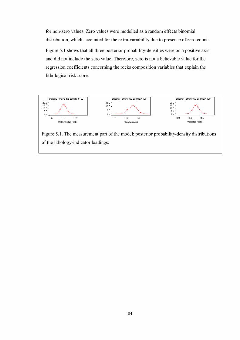
84

Figure 5.1. The measurement part of the model: posterior probability-density distributions

of the lithology-indicator loadings.

for non-zero values. Zero values were modelled as a random effects binomial

distribution, which accounted for the extra-variability due to presence of zero counts.

Figure 5.1 shows that all three posterior probability-densities were on a positive axis

and did not include the zero value. Therefore, zero is not a believable value for the

regression coefficients concerning the rocks composition variables that explain the

lithological risk score.

85

Figure 5.2. The measurement part of the model: autocorrelation plots and Brooks-

Gelman-Rubin graphs for the lithology-indicator loadings.

Figure 5.2 shows how convergence was reached for the loading factors estimates in

the measurement part of the SEM, after using a thinning interval of 40. History plots

show how the three independent chains, for each one of the different factor loadings,

had eventually mixed adequately (Figure 5.3, with red, blue, and green-coloured

chains). The Monte Carlo error was no greater than 5% of the posterior standard

deviation, for all three factor-loading estimates (Table 5.2). That is to say, precision

was achieved to the aimed standard.

86

Figure 5.3. The measurement model. Lithology-indicator loadings:

history plots.

87

5.2.2 Structural model

Table 5.2 shows the results from the structural part of the SEM model. The posterior

mean values for the regression coefficients concerning the first two mortality causes,

COPD and larynx cancer, were -0.01 and -0.015, respectively. These results suggest a

negative association between the lithology score and mortality due to either COPD or

larynx cancer. However, inspection of their respective 95% credible intervals (95%

CIs) shows that they include zero as a likely value. Thus, the 95% CIs ranged from -

0.040 to 0.019 and from -0.044 to 0.015, for COPD and larynx cancer respectively.

The posterior mean value for the regression coefficient from lung-cancer mortality

data was positive (0.023). In addition, the 95% CI for the regression coefficient did not

include zero; it ranged from 0.011 to 0.035.

Lithology- score node

mean sd MC error 2.5% median 97.5% start sample

COPD -0.01018 0.01493 1.977E-4 -0.03991 -0.01014 0.01939 11001 30000

Larynx

cancer -0.01513 0.01486 1.964E-4 -0.04442 -0.01523 0.01453 11001 30000

Lung

cancer 0.02252 0.006198 8.384E-5 0.0107 0.02242 0.03483 11001 30000

Table 5.2. Structural Model: lithology-score regression coefficients estimates for Chronic

Obstructive Pulmonary Disease (COPD), larynx cancer, and lung-cancer mortality, in men.

88

Figure 5.4. The structural part of the model: posterior probability-densities for the Relative

Risk (RR) of mortality explained by the lithology score, in the modelling of Chronic

Obstructive Pulmonary Disease (COPD), larynx cancer and lung cancer, in men.

Upper row: posterior probability-densities for RR explained by the lithology score, in

three different diseases (log scale).

Middle row: proportions of the posterior probability-densities for ln(RR) being zero or less

(0), or greater than zero (1).

Lower row: posterior probability-densities for RR explained by the lithology score –ratio

scale.

As a visual aid to interpretation, the whole posterior probability density for the

lithology score (for all three mortality causes) can be assessed in Figure 5.4. The upper

and bottom rows show the densities on the logarithmic and the ratio scale (RR),

respectively. It can be seen that the first two densities included the null value (zero on

the log scale and one on the original, ratio scale) as a likely estimate. Conversely, the

whole posterior density concerning lung cancer did not include the null value. The

middle row in Figure 5.3 shows this fact more clearly. It depicts both the areas of the

respective curves at (or below) the null value (marked as ‘0’) and above the null value

89

(marked as ‘1’). It can be seen that the whole posterior regression-coefficient density

was above zero, or one on the ratio scale, only for lung-cancer. For the other two

mortality causes, the densities included the null value; moreover, the areas above the

null value were relatively small (24% and 16% for COPD and larynx-cancer,

respectively). Therefore, the distribution of lung-cancer deaths (but not COPD or

larynx-cancer deaths) was positively associated with the lithological risk score.

Table 5.4 presents posterior estimates for the regression coefficients accounting for

area-level deprivation. In contrast to the lithology score, the mean posterior values for

deprivation in all three diseases are positive; 0.037, 0.042 and 0.053 for COPD, larynx

cancer and lung cancer, respectively. Their 95% CIs range from 0.013 to 0.061, from

0.020 to 0.065 and from 0.044 to 0.062, for COPD, larynx cancer and lung cancer,

respectively. Therefore, there is evidence of a positive association between the SES

scoring (deprivation) and all three of the mortality causes.

Deprivation-score node mean sd MC error 2.5% median 97.5% start sample

COPD 0.03681 0.01216 2.576E-4 0.01315 0.03672 0.06097 11001 30000

Larynx cancer 0.04221 0.01164 2.18E-4 0.01975 0.04224 0.06523 11001 30000

Lung cancer 0.05301 0.00475 1.037E-4 0.0437 0.05295 0.06242 11001 30000

Table 5.3 The structural part of the model: estimates for the deprivation-score regression

coefficients. Chronic Obstructive Pulmonary Disease (COPD), larynx cancer, and lung-cancer

mortality, in men.

90

The same interpretation can be drawn from the shape of their whole posterior densities

shown in Figure 5.5. The upper and bottom rows show the probability densities on the

log and ratio (Relative Risk -RR) scales, respectively. It can be seen that none of the

densities for all three diseases (COPD, larynx and lung cancer) included the null value.


relative risk (RR) explained by the deprivation-score.

Upper row: posterior probability-densities for the RR explained by the deprivation-

score, in all three different diseases: Chronic Obstructive Pulmonary Disease (COPD),

larynx cancer, and lung cancer; log scale.

Middle row: proportions of the posterior probability-densities for ln(RR) being zero or

less (0), or greater than zero (1).

Lower row: posterior probability-densities for The RR explained by the deprivation

score.

91

This is also depicted by the graphs in the middle row (Figure 5.4) where the whole

area under the density curve is marked as 1 (as they were greater than the null value)

for all three diseases.

Lastly, Figure 5.6 provides additional assessment of convergence for deprivation

estimates. History plots show adequate mixing of the three independent chains in all

the three cases (COPD, larynx and lung cancer). The BGR diagnostic graph also

shows that the BGR ratio statistic (in the colour red) had stabilised close to the value

of one. All these diagnostic criteria helped in demonstrating that the posterior

estimates had been drawn from the target distribution.

Figure 5.6. The structural part of the model: convergence of the deprivation-score

estimates.

From top to bottom, history-plots (first column) and Brooks-Gelman-Rubin graphs

(second column) for the deprivation-score regression coefficients in modelling of

Chronic Obstructive Pulmonary Disease (COPD), larynx cancer and lung cancer,

respectively.

92

5.2.3 Summary of the Structural Equation Model

Presence of metamorphic, plutonic and volcanic rocks, are all features that correlate

well with a lithology score that presumes spatial similarity (autocorrelation) of nearby

geographical areas. Furthermore, this lithology score is positively associated with the

spatial distribution of deaths due to lung cancer in men, and the association remains

after controlling for deprivation in the model. The deprivation score turns out to also

be positively associated with the spatial distribution of male deaths due to lung cancer.

Similarly, there exists a positive association between deprivation and the spatial

distribution of deaths due to both COPD and larynx cancer. However, there is no

evidence of an association between lithology and the number of deaths due to either

COPD, or larynx cancer.

5.3 Lung-cancer mortality modelling

5.3.1 Besag-York-Mollié model: males

A BYM model was fitted to lung-cancer mortality data in men. The lithology score

derived from the SEM (see 5.2), as well as area-level deprivation were included in all

models. Five different models were simultaneously fitted: An intercept-only model

(model ‘y1’); intercept plus the lithology score (model ‘y2’); intercept, plus lithology

and deprivation scores (model ‘y3’); a further model that included a clustering

component (model ‘y4’), and the last one which also included a random-heterogeneity

component (model ‘y5’), which is the full BYM model. The relative merit of all these

models was assessed for both, the goodness of fit of observed data as well as their

predictive ability. To assess the relative goodness of fit of the observed data, the

Deviance Information Criterion (DIC) was used to determine the optimal model. The

model with the smallest DIC value was chosen as the best fitting model amongst those

compared. This model (Table 5.4) turned out to be the full BYM model with the

lithology and deprivation scores included (model ‘y5’). In this case, the DIC was

4,050, much lower than the second best one (model ‘y4’) which gave a DIC value of

4,552.

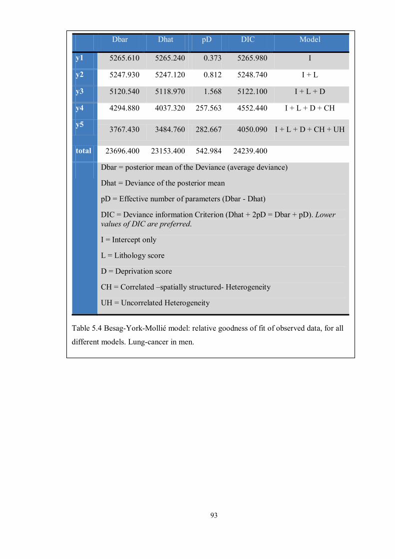
93

Dbar Dhat pD DIC Model

y1 5265.610 5265.240 0.373 5265.980 I

y2 5247.930 5247.120 0.812 5248.740 I + L

y3 5120.540 5118.970 1.568 5122.100 I + L + D

y4 4294.880 4037.320 257.563 4552.440 I + L + D + CH

y5 3767.430 3484.760 282.667 4050.090 I + L + D + CH + UH

total 23696.400 23153.400 542.984 24239.400

Dbar = posterior mean of the Deviance (average deviance)

Dhat = Deviance of the posterior mean

pD = Effective number of parameters (Dbar - Dhat)

DIC = Deviance information Criterion (Dhat + 2pD = Dbar + pD). Lower values of DIC are preferred.

I = Intercept only

L = Lithology score

D = Deprivation score

CH = Correlated –spatially structured- Heterogeneity

UH = Uncorrelated Heterogeneity

Table 5.4 Besag-York-Mollié model: relative goodness of fit of observed data, for all

different models. Lung-cancer in men.

94

To assess the relative predictive ability of the different models two different loss

functions were used that measured the difference between the observed and the

predicted values (also known as Posterior Predictive Loss). The loss functions used

were the Mean Square Predictive Error (MSPE), which is shown in Table 5.5, and the

Mean Absolute Predictive Error (MAPE), in Table 5.6. As for the DIC, the model with

the smallest value (either for the MSPE or the MAPE) is preferred. The model with the

lowest MSPE value was the full BYM model (model ‘y5’, MSPE = 65), while the

second best one (model ‘y4’) had a much larger value (MSPE = 782). Models were

ranked the same way when the MAPE was taken into consideration. The full BYM

model (‘y5’) had a posterior mean MAPE value of 4.6, while the second best model

(‘y4’, which was the one without the random-heterogeneity component) had a value of

7.2. Therefore, the full BYM gave the best fit for both the observed values and the

predicted ability. The Posterior Predictive Loss (PPL) can also be used as a mean to

assess convergence. Table 5.5 and Table 5.6 show that the Monte Carlo error (MC

error) for both the MSPE and MAPE estimates (and all the models compared) was

around 1% of their posterior standard-deviation estimates, which demonstrates that

convergence had been achieved; this is required for the estimates to arise from the

target distribution.

95

MSPE mean sd MC error

2.5% median 97.5% start sample Model

y1 403.1 50.22 0.3613 310.9 400.5 507.8 1001 21990 I

y2 419.1 52.1 0.362 324.9 416.5 527.9 1001 21990 I + L

y3 224.0 27.82 0.1895 175.8 222.0 284.7 1001 21990 I + L + D

y4 782.3 170.0 2.265 483.2 770.6 1149.0 1001 21990 I + L + D + CH

y5 65.05 14.06 0.09957 45.05 62.53 99.29 1001 21990 I + L + D + CH + UH

MSPE = Mean Squared Predictive Error. Lower values of MSPE are preferred.

I = Intercept only

L = Lithology score


CH = Correlated Heterogeneity


Table 5.5 Besag-York-Mollié model. Relative goodness of predictive ability (MSPE) for all

different models. Lung cancer in men.

96

MAPE mean sd MC error 2.5% median 97.5% start sample Model y1 7.722 0.1767 0.001221 7.378 7.723 8.07 1001 21990 I y2 7.68 0.1779 0.001232 7.331 7.679 8.032 1001 21990 I + L y3 7.174 0.18 0.001173 6.825 7.175 7.526 1001 21990 I + L + D y4 7.167 0.3873 0.005444 6.427 7.159 7.941 1001 21990 I + L + D +

CH y5 4.545 0.1834 0.001524 4.199 4.54 4.914 1001 21990 I + L + D +

CH + UH MAPE = Mean Absolute Predictive Error. Lower values of MAPE are preferred.

I = Intercept only

L = Lithology score




Table 5.6 Besag-York-Mollié model. Relative goodness of predictive ability (MAPE) for all

different models. Lung cancer in men.

97

Once the model had converged, posterior estimates were obtained for the regression

coefficients for both the lithology and deprivation scores. The posterior mean-

estimates on the log scale were 0.023 and 0.04 for the lithology and deprivation

scores, respectively. Their respective 95% CIs ranged from 0.015 to 0.031 and 0.033

to 0.046 (Table 5.7). An interaction term between the lithology score and area-level

deprivation (as surrogate measures for potential radon-gas exposure and tobacco

smoking, respectively) did not improve the goodness of fit of the model; the mean

posterior estimate for the interaction term was -0.001 with 95% CI [-0.002, 0.002].

Therefore, there is a positive association between the lithology score and mortality due

to lung cancer in men. There is also a positive association between the deprivation

score and lung cancer mortality in men. The same interpretation can be seen on the

ratio (RR) scale. The computed posterior mean-values were 1.02 and 1.04 for the

lithology and deprivation scores, respectively. Their respective posterior 95% CIs

varied from 1.015 to 1.031 for the former and 1.033 to 1.048 for the latter (Table 5.8).

Node mean sd MC error 2.5% median 97.5% start sample

Intercept 0.01229 0.004091 3.664E-5 0.004321 0.01227 0.02027 8331 38010

Lithology 0.02292 0.00389 3.166E-5 0.0153 0.02291 0.03051 8331 38010

Deprivation 0.03953 0.003565 4.049E-5 0.03257 0.03955 0.04647 8331 38010

Table 5.7 Besag-York-Mollié model. Regression-coefficients estimates (log scale). Lung-

cancer in men.

Node mean sd MC error 2.5% median 97.5% start sample Lithology 1.023 0.00398 3.24E-5 1.015 1.023 1.031 8331 38010 Deprivation 1.04 0.003709 4.212E-5 1.033 1.04 1.048 8331 38010

Table 5.8 Besag-York-Mollié model: regression-coefficients estimates (ratio scale). Lung-

cancer in men.

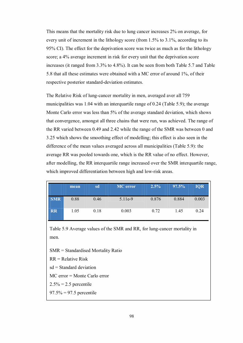
98

This means that the mortality risk due to lung cancer increases 2% on average, for

every unit of increment in the lithology score (from 1.5% to 3.1%, according to its

95% CI). The effect for the deprivation score was twice as much as for the lithology

score; a 4% average increment in risk for every unit that the deprivation score

increases (it ranged from 3.3% to 4.8%). It can be seen from both Table 5.7 and Table

5.8 that all these estimates were obtained with a MC error of around 1%, of their

respective posterior standard-deviation estimates.

The Relative Risk of lung-cancer mortality in men, averaged aver all 759

municipalities was 1.04 with an interquartile range of 0.24 (Table 5.9); the average

Monte Carlo error was less than 5% of the average standard deviation, which shows

that convergence, amongst all three chains that were run, was achieved. The range of

the RR varied between 0.49 and 2.42 while the range of the SMR was between 0 and

3.25 which shows the smoothing effect of modelling; this effect is also seen in the

difference of the mean values averaged across all municipalities (Table 5.9): the

average RR was pooled towards one, which is the RR value of no effect. However,

after modelling, the RR interquartile range increased over the SMR interquartile range,

which improved differentiation between high and low-risk areas.

mean sd MC error 2.5% 97.5% IQR

SMR 0.88 0.46 5.11e-9 0.876 0.884 0.003

RR 1.05 0.18 0.003 0.72 1.45 0.24

Table 5.9 Average values of the SMR and RR, for lung-cancer mortality in

men.

SMR = Standardised Mortality Ratio

RR = Relative Risk

sd = Standard deviation

MC error = Monte Carlo error

2.5% = 2.5 percentile

97.5% = 97.5 percentile

99

Figure 5.7 to Figure 5.14 show the distribution of posterior RR estimates across all

759 municipalities analysed, while being grouped by provinces. Box plots limits

represent the posterior quartiles; the middle bars within the boxes are the posterior

mean values, and the whisker lines reach the 2.5% and 97.5% posterior percentiles.

The reference line represents the posterior mean which was averaged over all

municipalities (within each province). It can be seen that the mean posterior RR were

highest in the provinces of Cádiz (mean RR 1.35; Figure 5.8), Sevilla (mean RR 1.34;

Figure 5.14) and Huelva (mean RR 1.15; Figure 5.11) while they were lowest in the

provinces of Jaén (mean RR 0.80; Figure 5.12) and Granada (mean RR 0.89; Figure

5.10). However, there was ample heterogeneity within provinces and the RR estimates

which represent lower and higher risk than the average value, for any particular

province, can be clearly identified from their individual box plots, as their green areas

represent 95% CI.

Almería province (mean baseline Relative Risk = 1.03)

Relative Risk 0.0 1.0 2.0 3.0 4.0

Figure 5.7. Ranking of posterior estimates of Relative Risk boxplots, for all

101 muncipalities in the province of Almería. Lung-cancer in men.

100

Cádiz province (mean baseline Relative Risk = 1.35)

Relative Risk 0.5 1.0 1.5 2.0 2.5


42 muncipalities in the province of Cádiz. Lung-cancer in men.

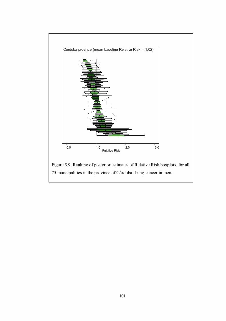
101

Córdoba province (mean baseline Relative Risk = 1.02)

Relative Risk 0.0 1.0 2.0 3.0


75 muncipalities in the province of Córdoba. Lung-cancer in men.

102

Granada province (mean baseline Relative Risk = 0.89)


Figure 5.10. Ranking of posterior estimates of Relative Risk boxplots, for

all 166 muncipalities in the province of Granada. Lung-cancer in men.

103

Huelva province (mean baseline Relative Risk = 1.15)



all 79 muncipalities in the province of Huelva. Lung-cancer in men.

104

Jaén province (mean baseline Relative Risk = 0.8)

Relative Risk 0.0 0.5 1.0 1.5 2.0


all 96 muncipalities in the province of Jaén. Lung-cancer in men.

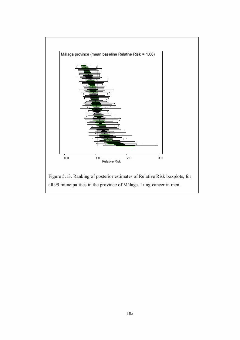
105

Málaga province (mean baseline Relative Risk = 1.08)



all 99 muncipalities in the province of Málaga. Lung-cancer in men.

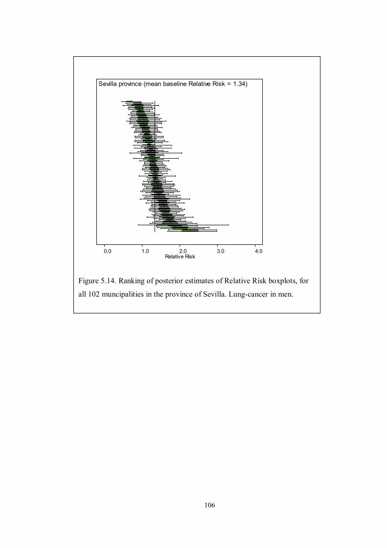
106

Sevilla province (mean baseline Relative Risk = 1.34)

Relative Risk 0.0 1.0 2.0 3.0 4.0


all 102 muncipalities in the province of Sevilla. Lung-cancer in men.

107

The frequency distribution of the observed number of lung-cancer cases in men was

overdispersed (ratio variance/mean = 518.3; Bohning’s statistic 53.81, p value <

0.001). Therefore, further analysis was implemented for checking if overdisperion was

only due to unstructured heterogeneity (e.g., because of excess of zero counts: 4.4% of

all records in the male lung-cancer dataset) or spatial autocorrelation was also present.

A Moran’s I Monte Carlo test was run as well within R software, for testing the spatial

dependency of the SMRs distribution; the adjacency matrix was used as weights for

this test (Moran’s I statistic = 0.25 after 1,000 simulations, p value = 0.001). Given

that spatial autocorrelation was present, a hierarchical BYM model was fitted

afterwards, where separate estimates for the residual variance components were

computed: namely, spatially-correlated (clustering) and uncorrelated (random)

heterogeneity. This allowed for the Variance Partition Coefficient (VPC) to be

calculated. The posterior mean estimate of the VPC was 0.95 and its posterior 95% CI

ranged from 0.93 to 0.97 (Table 5.10).

Consequently, most (95%) of the residual variance (not explained by the model) was

due to spatial autocorrelation of the estimates amongst nearby municipalities, and just

a small amount (5%) was due to random variability within geographical areas.

Therefore, most of the variability not explained by the model was due to (unmeasured)

factors that vary across geographical areas.

5.3.2 Besag-York-Mollié model: females

The same BYM model previously used (see 5.3.1) was applied to model mortality due

to lung-cancer in women. Five different models were also adjusted and simultaneously

compared. From the simplest to the most complex one, those models were: an

intercept-only model (‘y1’); model ‘y2’, which added the lithology score to the

Node mean sd MC error

2.5% median 97.5% start sample

VPC 0.9541 0.009781 2.011E-4 0.9326 0.9552 0.9708 41001 2742

Table 5.10. Besag-York-Mollié model: Variance Partition Coefficient (VPC) estimates.

Lung-cancer in men.

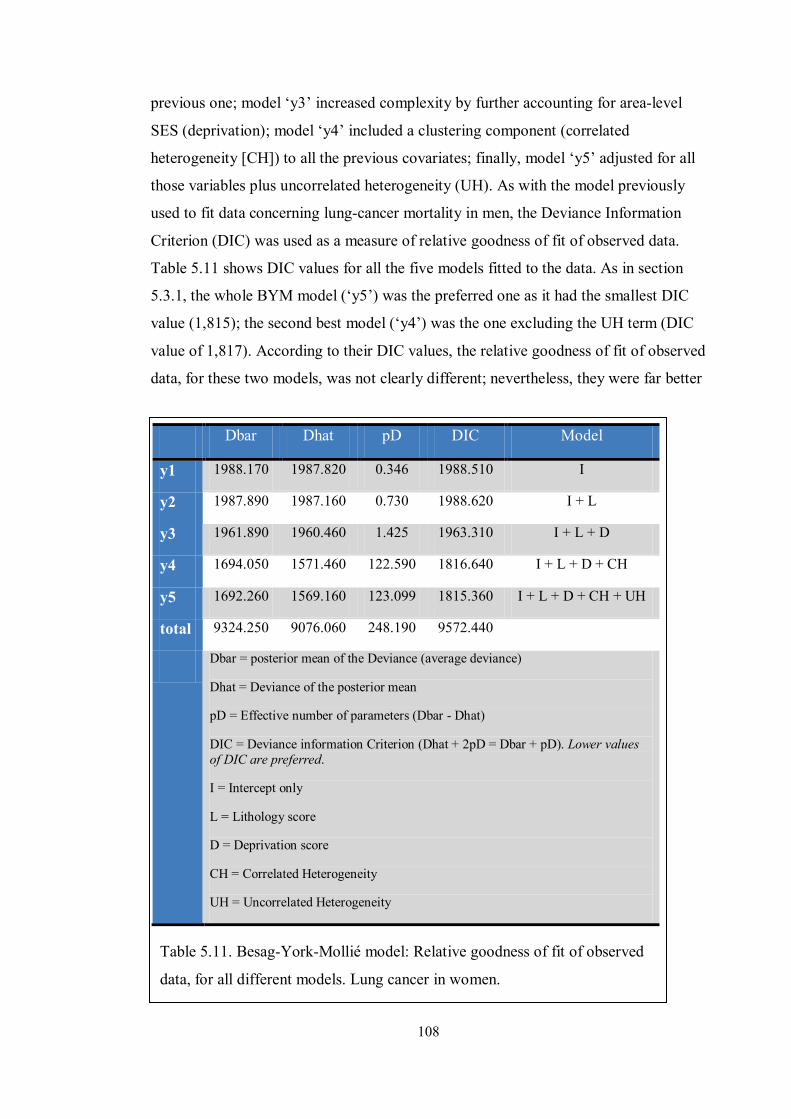
108

previous one; model ‘y3’ increased complexity by further accounting for area-level

SES (deprivation); model ‘y4’ included a clustering component (correlated

heterogeneity [CH]) to all the previous covariates; finally, model ‘y5’ adjusted for all

those variables plus uncorrelated heterogeneity (UH). As with the model previously

used to fit data concerning lung-cancer mortality in men, the Deviance Information

Criterion (DIC) was used as a measure of relative goodness of fit of observed data.

Table 5.11 shows DIC values for all the five models fitted to the data. As in section

5.3.1, the whole BYM model (‘y5’) was the preferred one as it had the smallest DIC

value (1,815); the second best model (‘y4’) was the one excluding the UH term (DIC

value of 1,817). According to their DIC values, the relative goodness of fit of observed

data, for these two models, was not clearly different; nevertheless, they were far better

Dbar Dhat pD DIC Model

y1 1988.170 1987.820 0.346 1988.510 I

y2 1987.890 1987.160 0.730 1988.620 I + L

y3 1961.890 1960.460 1.425 1963.310 I + L + D

y4 1694.050 1571.460 122.590 1816.640 I + L + D + CH

y5 1692.260 1569.160 123.099 1815.360 I + L + D + CH + UH

total 9324.250 9076.060 248.190 9572.440

Dbar = posterior mean of the Deviance (average deviance)

Dhat = Deviance of the posterior mean

pD = Effective number of parameters (Dbar - Dhat)

DIC = Deviance information Criterion (Dhat + 2pD = Dbar + pD). Lower values of DIC are preferred.

I = Intercept only

L = Lithology score




Table 5.11. Besag-York-Mollié model: Relative goodness of fit of observed

data, for all different models. Lung cancer in women.

109

than models ‘y1’, ‘y2’ (DIC values of 1,989 for both models) and ‘y3’ (DIC of 1,963).

Goodness of fit of predicted values was also assessed by means of loss type functions:

Table 5.12 shows estimates of the Mean Square Predictive Error (MSPE) for each

model. The lowest (preferred) values happened for models ‘y4’ and ‘y5’ (mean

estimated value of around 6, for both models); while the estimates for model ‘y3’

(MSPE = 7) and models ‘y1’ and ‘y2’ (MSPE = 10) were higher.

Table 5.13 shows posterior estimates for a second form of loss function (Mean

Absolute Predictive Error [MAPE]). Again, the lowest mean values were obtained for

MSPE mean sd MC error 2.5% median 97.5% start sample Model

y1 10.69 2.33 0.01403 6.754 10.48 15.84 1001 30000 I

y2 10.59 2.335 0.01516 6.697 10.37 15.8 1001 30000 I + L

y3 6.924 1.34 0.007901 4.864 6.735 10.04 1001 30000 I + L + D

y4 6.036 2.164 0.02011 3.378 5.514 11.57 1001 30000 I + L + D + CH

y5 5.573 1.788 0.01544 3.335 5.154 10.14 1001 30000 I + L + D + CH + UH

MSPE = Mean Squared Predictive Error. Lower values of MSPE are preferred.

I = Intercept only

L = Lithology score



UH = Uncorrelated Heterogeneity.

Table 5.12. Besag-York-Mollié model: relative goodness of predictive ability (MSPE) for all

different models. Lung-cancer in women.

MAPE mean sd MC error

2.5% median 97.5% start sample Model

y1 1.361 0.04935 2.787E-4 1.265 1.361 1.458 1001 30000 I

y2 1.359 0.04883 3.03E-4 1.264 1.358 1.456 1001 30000 I + L

y3 1.311 0.0493 2.764E-4 1.216 1.31 1.408 1001 30000 I + L + D

y4 1.154 0.05856 4.505E-4 1.045 1.152 1.275 1001 30000 I + L + D + CH

y5 1.146 0.0562 3.81E-4 1.041 1.144 1.262 1001 30000 I + L + D + CH + UH

MAPE = Mean Absolute Predictive Error. Lower values of MAPE are preferred.

I = Intercept only

L = Lithology score




Table 5.13. Besag-York-Mollié model: Relative goodness of predictive ability (MAPE) for

the different models. Lung cancer in women.

110

model ‘y5’ and ‘y4 (MAPE = 1.1 and 1.2, respectively). The estimated MAPE was 1.4

for both models ‘y1’ and ‘y2’, and 1.3 for model ‘y3’. All these results (DIC, MSPE

and MAPE) showed that the BYM model was the best one (amongst those compared)

to fit lung-cancer mortality data in women. However, there was not much difference

between the model adjusting for both correlated (CH) and uncorrelated (UH)

heterogeneity and the one including only a CH term (plus lithology and deprivation as

covariates).

111

Figure 5.15. Besag-York-Mollié model: posterior probability-densities for

lithology and deprivation. Lung-cancer in women.

Upper row: lithology (beta) and deprivation (delta) scores: posterior probability-

density distributions (log scale).

Middle row: Proportions of the posterior probability-densities for the regression

coefficients being zero or less (0), or greater than zero (1): Probability(lithology-

score) >0 = 0.8973. Modelling of lung-cancer deaths in women.

Lower row: regression coefficients (ratio scale).

A visual guide for the relevance and magnitude of both the lithology and deprivation

scores is given in Figure 5.16. The first and last rows in this graph show the posterior

probability-densities for both variables, on a linear and ratio (RR) scales, respectively.

In contrast to the results obtained from fitting the BYM model to the male dataset, the

posterior probability density for the lithology score includes the null value (zero, or

one, on the linear and ratio scales, respectively).

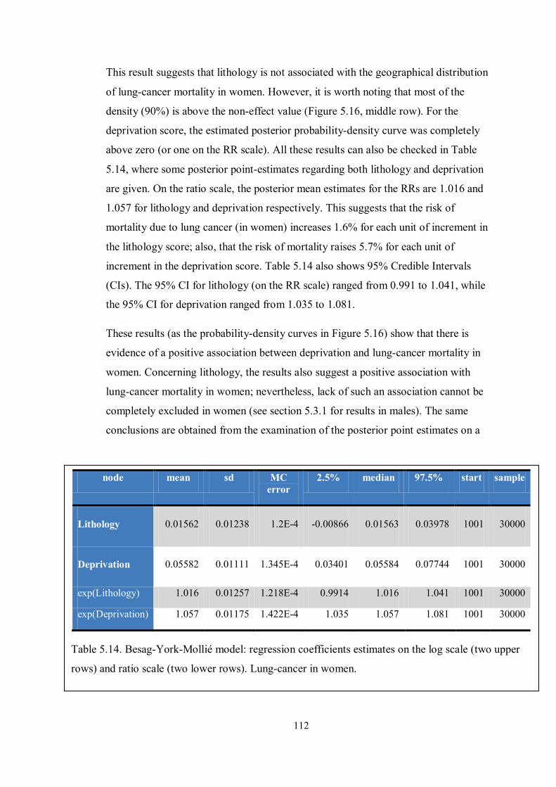
112

This result suggests that lithology is not associated with the geographical distribution

of lung-cancer mortality in women. However, it is worth noting that most of the

density (90%) is above the non-effect value (Figure 5.16, middle row). For the

deprivation score, the estimated posterior probability-density curve was completely

above zero (or one on the RR scale). All these results can also be checked in Table

5.14, where some posterior point-estimates regarding both lithology and deprivation

are given. On the ratio scale, the posterior mean estimates for the RRs are 1.016 and

1.057 for lithology and deprivation respectively. This suggests that the risk of

mortality due to lung cancer (in women) increases 1.6% for each unit of increment in

the lithology score; also, that the risk of mortality raises 5.7% for each unit of

increment in the deprivation score. Table 5.14 also shows 95% Credible Intervals

(CIs). The 95% CI for lithology (on the RR scale) ranged from 0.991 to 1.041, while

the 95% CI for deprivation ranged from 1.035 to 1.081.

These results (as the probability-density curves in Figure 5.16) show that there is

evidence of a positive association between deprivation and lung-cancer mortality in

women. Concerning lithology, the results also suggest a positive association with

lung-cancer mortality in women; nevertheless, lack of such an association cannot be

completely excluded in women (see section 5.3.1 for results in males). The same

conclusions are obtained from the examination of the posterior point estimates on a

node mean sd MC error

2.5% median 97.5% start sample

Lithology 0.01562 0.01238 1.2E-4 -0.00866 0.01563 0.03978 1001 30000

Deprivation 0.05582 0.01111 1.345E-4 0.03401 0.05584 0.07744 1001 30000

exp(Lithology) 1.016 0.01257 1.218E-4 0.9914 1.016 1.041 1001 30000

exp(Deprivation) 1.057 0.01175 1.422E-4 1.035 1.057 1.081 1001 30000

Table 5.14. Besag-York-Mollié model: regression coefficients estimates on the log scale (two upper

rows) and ratio scale (two lower rows). Lung-cancer in women.

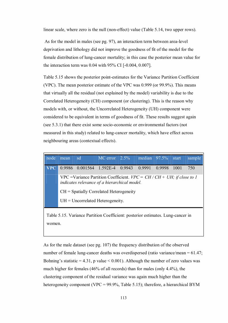
113

linear scale, where zero is the null (non-effect) value (Table 5.14, two upper rows).

As for the model in males (see pg. 97), an interaction term between area-level

deprivation and lithology did not improve the goodness of fit of the model for the

female distribution of lung-cancer mortality; in this case the posterior mean value for

the interaction term was 0.04 with 95% CI [-0.004, 0.007].

Table 5.15 shows the posterior point-estimates for the Variance Partition Coefficient

(VPC). The mean posterior estimate of the VPC was 0.999 (or 99.9%). This means

that virtually all the residual (not explained by the model) variability is due to the

Correlated Heterogeneity (CH) component (or clustering). This is the reason why

models with, or without, the Uncorrelated Heterogeneity (UH) component were

considered to be equivalent in terms of goodness of fit. These results suggest again

(see 5.3.1) that there exist some socio-economic or environmental factors (not

measured in this study) related to lung-cancer mortality, which have effect across

neighbouring areas (contextual effects).

As for the male dataset (see pg. 107) the frequency distribution of the observed

number of female lung-cancer deaths was overdispersed (ratio variance/mean = 61.47;

Bohning’s statistic = 4.31, p value < 0.001). Although the number of zero values was

much higher for females (46% of all records) than for males (only 4.4%), the

clustering component of the residual variance was again much higher than the

heterogeneity component (VPC = 99.9%, Table 5.15); therefore, a hierarchical BYM

node mean sd MC error 2.5% median 97.5% start sample

VPC 0.9986 0.001564 1.592E-4 0.9943 0.9991 0.9998 1001 750

VPC =Variance Partition Coefficient. VPC = CH / CH + UH; if close to 1 indicates relevance of a hierarchical model.

CH = Spatially Correlated Heterogeneity

UH = Uncorrelated Heterogeneity.

Table 5.15. Variance Partition Coefficient: posterior estimates. Lung-cancer in

women.

114

Figure 5.16. Standardised Mortality Ratio estimates for lung-cancer mortality in

men.

(34) < 0.0

(440) 0.0 - 1.0

(273) 1.0 - 2.0

(11) 2.0 - 3.0

(1) >= 3.0

(samples)means for SMR

200.0km

N

model was again justified, as spatial autocorrelation, rather than random heterogeneity,

seemed to be responsible for virtually all overdispersion.

5.3.3 Mapping of lung-cancer mortality modelling: males

Figure 5.17 shows the Standardised Mortality Ratios (SMRs) due to lung-cancer

mortality in men. It represents the observed (that is, before modelling) SMRs values,

where there is a high concentration of municipalities with values greater than one to

the west of the region, as reported by previous studies.

To distinguish between observed SMRs values and posterior (modelled) estimates, the

latter had been labelled as Relative Risks (RR). To visually appraise the relative

magnitude of each model component (see 5.3), mapping of RR of lung-cancer

mortality in men was implemented by taking into consideration all the modelling

components and, separately, each one of them. Figure 5.18 maps the posterior lung-

cancer RR estimates in men, for each one of the 759 municipalities in the whole

region. These estimates were obtained from the full BYM model that accounted for

both lithology and deprivation scores. The model also included a variance component

that comprised spatial autocorrelation and random heterogeneity.

115

Figure 5.18 gives the number of municipalities (within parenthesis) for each RR cut-

off point. It can be seen that amongst municipalities with a high-risk of mortality, 323

(84%) had an estimated RR up to 50% higher than expected. 53 municipalities (14%)

had an RR of lung-cancer mortality which was up to 100% above expectation. Finally,

only 7 municipalities (2%) had an increased RR beyond 100% of expected.

To aid interpretation of these estimates, Figure 5.19 presents an exceedance-

probabilities map. Given that the whole posterior RR density was available for every

municipality, it was possible to compute the area under the curve lies above some

specific value. In this case, the map was devised to classify the municipalities

according to the probability that its estimated RRs were greater than 1, which is the

null RR. The more area under the RR curve would lie above the value of 1, the more

the hypothesis of an RR greater than expected would be supported. This map (Figure

5.19) shows that there were 47 municipalities for which the probability of an RR

greater than 1 ranged between 0.75 and 0.85; another 59 areas had a probability of an

excessive risk between 0.85 and 0.95; in another 50 areas that probability varied

between 0.95 and 0.99. Lastly, for 105 further areas the probability of an excessive

risk was virtually 1; in other words, for each of these 105 municipalities, all of the area

belonging to their respective posterior RR probability-density curves was situated

Figure 5.17. Posterior Relative Risks of lung-cancer mortality in men.

(1) < 0.5

(375) 0.5 - 1.0

(323) 1.0 - 1.5

(53) 1.5 - 2.0

(7) >= 2.0

(samples)means for RR

200.0km

N

116

above the value of 1.This smoothed exceedance-probabilities map clearly shows how

municipalities with higher risk concentrated to the west of the region, as reported in

previous studies [10, 13].


cancer mortality in men.

(498) < 0.75

(47) 0 .75 - 0 .85

(59) 0 .85 - 0 .95

(50) 0 .95 - 0 .99

(105) >= 0 .99

probability of RR greater than 1.0

200.0km

N

117

Later in this section (pg. 124), it will be explained that clustering is the model

component responsible for this spatial pattern. A mirror image of the previous map is

given by Figure 5.20, which gives, for each municipality, the probability of their RR

being less than expected. It shows that the areas with the highest probability of their

posterior RRs being less than 1 are concentrated to the east of Andalucía.



(480) < 0.75

(66) 0 .75 - 0 .85

(96) 0 .85 - 0 .95

(53) 0 .95 - 0 .99

(64) >= 0.99

probability of RR less than 1.0

200.0km

N

118

To further analyse the fitted model, mapping was presented separately for each model

component. Figure 5.21 represents the RR explained only by lithology scores, where

401 municipalities out of a total of 759 (or 53%) were classified as areas with an RR

(due to lithology) greater than expected. Of these high risk areas, 301 (75%) had an

RR up to 2.5% higher than expected; 100 municipalities (25%) had an RR greater that

2.5% above expectation.

Figure 5.20. Relative Risks explained by lithology scores. Lung-cancer mortality in

men.

(13) < 0.95

(91) 0.95 - 0.975

(254) 0.975 - 1.0

(301) 1.0 - 1.025

(100) >= 1.025

(samples)means for RR_litho

200.0km

N

119

The corresponding exceedance-probabilities map (Figure 5.22) shows that 401

municipalities (or 53%) had RR estimates for which virtually all their probability-

density curves were above the value of 1. These geographical areas were mainly

situated on two separated strips across the north and south of the region.

Figure 5.21. Exceedance-probabilities map for lithology scores (Probability

[Relative Risk > 1]). Lung-cancer mortality in men.

(358) < 0.75

(0) 0.75 - 0 .85

(0) 0.85 - 0 .95

(0) 0.95 - 0 .99

(401) >= 0 .99

probability of RR_litho greater than 1.0

200.0km

N

120

The complementary map (Figure 5.23) shows the areas (a middle band across the

whole region) where the probabilities of an RR, due to lithology, being less than 1

were higher.

Figure 5.22. Exceedance-probabilities map for lithology scores (Probability

[Relative Risk < 1]). Lung-cancer mortality in men.

(401) < 0.75

(0) 0.75 - 0 .85

(0) 0.85 - 0 .95

(0) 0.95 - 0 .99

(358) >= 0 .99

probability of RR_litho less than 1.0

200.0km

N

121

A second RR component individually analysed was SES at area level, which was

represented by the deprivation score. Figure 5.24 displays 361 geographical areas out

of a total number of 759 (or 48%) that showed an RR –due to deprivation- greater than

1. Within all these high-deprivation areas, 334 municipalities (93%) had an excess of

risk up to 10% greater than expected. Only 27 areas (or 7%) had a risk increased

above 10% of expectation.

Figure 5.23. Relative Risks explained by deprivation scores. Lung-cancer mortality

in men.

(14) < 0.9

(384) 0.9 - 1.0

(334) 1.0 - 1.1

(27) >= 1 .1

(samples )means for RR_depriv

200.0km

N

122

Exceedance-probabilities maps for the RR due to deprivation are shown in Figure 5.25

(for an RR greater than 1) and Figure 5.26 (for an RR less than 1). There were 361

municipalities (48%) for which the probability of an RR being greater than expected

was virtually 1 (or 100%). Unlike the risk associated with the lithology component,

the one due to deprivation does not seem to concentrate on any particular area. The

clustering component was actually not captured by either of the two explanatory

variables (lithology or deprivation) included in the model.



(398) < 0.75

(0) 0.75 - 0 .85

(0) 0.85 - 0 .95

(0) 0.95 - 0 .99

(361) >= 0 .99

probability of RR_depriv greater than 1.0

200.0km

N

123


[Relative Risk < 1]). Lung-cancer mortality in men.

(361) < 0.75

(0) 0.75 - 0 .85

(0) 0.85 - 0 .95

(0) 0.95 - 0 .99

(398) >= 0 .99

probability of RR_depriv less than 1.0

200.0km

N

124

The residual RR and its two components (clustering and heterogeneity) was the third

(and last) RR component analysed. Figure 5.27 shows the map of posterior RR

estimates due to the residual variability. In this map, 317 geographical areas of high-

risk of mortality (or 83%) had a risk which increased up to 50% beyond expected (RR

from 1 to 1.5). 58 areas (15%) had an increment in risk between 50% and up to 100%

(RR between 1.5 and 2). 6 areas (2%) showed a risk increment greater than 100% (RR

greater than 2). The map exhibiting the residual RR is very similar to the one showed

in Figure 5.18, which took into consideration all the explanatory variables plus the

residual-variance components. This shows that the factor responsible for this

characteristic spatial pattern of mortality was not captured by any of the two

explanatory variables included in the model.

Figure 5.26. Residual Relative Risks. Lung-cancer mortality in men.

(2) < 0 .5

(376) 0.5 - 1.0

(317) 1.0 - 1.5

(58) 1 .5 - 2 .0

(6) >= 2.0

(samples )means for res_RR

200.0km

N

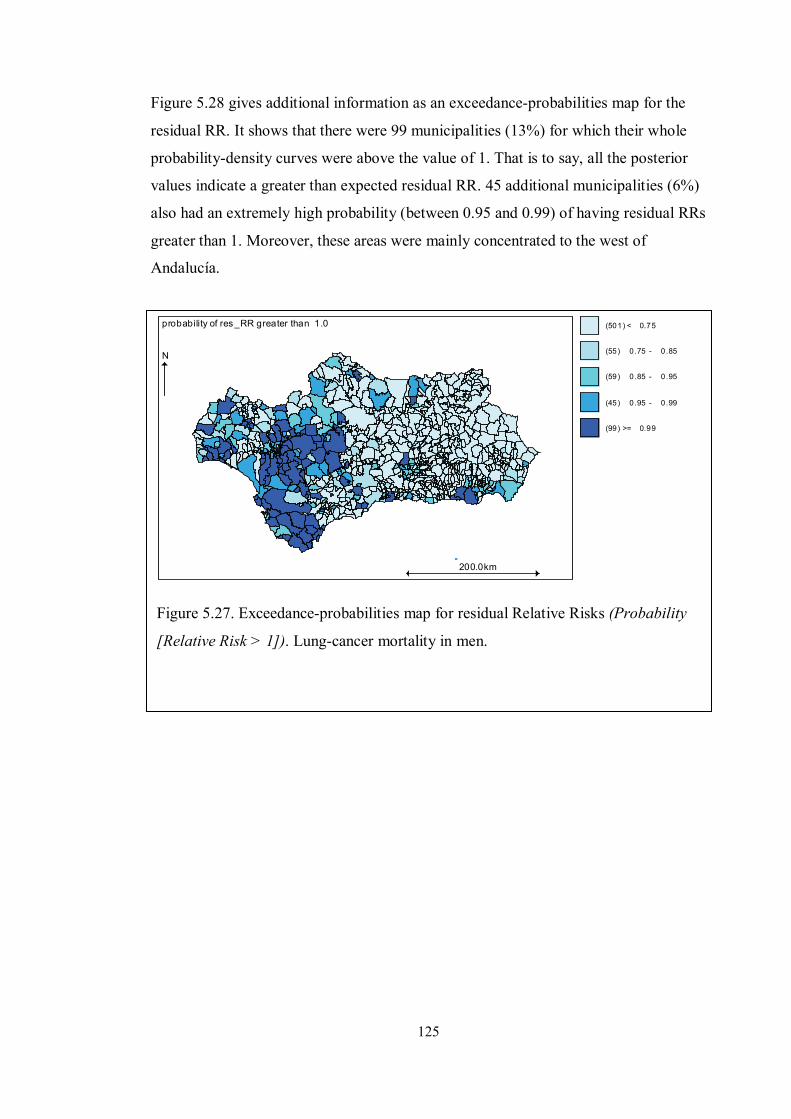
125

Figure 5.28 gives additional information as an exceedance-probabilities map for the

residual RR. It shows that there were 99 municipalities (13%) for which their whole

probability-density curves were above the value of 1. That is to say, all the posterior

values indicate a greater than expected residual RR. 45 additional municipalities (6%)

also had an extremely high probability (between 0.95 and 0.99) of having residual RRs

greater than 1. Moreover, these areas were mainly concentrated to the west of

Andalucía.

Figure 5.27. Exceedance-probabilities map for residual Relative Risks (Probability


(501) < 0.75

(55) 0 .75 - 0 .85

(59) 0 .85 - 0 .95

(45) 0 .95 - 0 .99

(99) >= 0.99

probability of res_RR greater than 1.0

200.0km

N

126

An opposite pattern is shown in Figure 5.29, which presents an exceedance-

probabilities map of the residual RR being less than 1. It can be seen that 56

geographical areas (7%) had virtually all their residual-RR curves below the null

value, while for 62 additional municipalities (8%), between 95% and 99% of the area

of their probability-density curves were below the value of 1. In contrast to the

previous map (Figure 5.28) these low-probability risk areas are mainly concentrated to

the east of Andalucía.

Figure 5.28. Exceedance-probabilities map for the residual Relative Risks

(Probability [Relative Risk < 1]). Lung-cancer mortality in men.

(488) < 0.75

(60) 0 .75 - 0 .85

(93) 0 .85 - 0 .95

(62) 0 .95 - 0 .99

(56) >= 0.99

probability of res_RR less than 1.0

200.0km

N

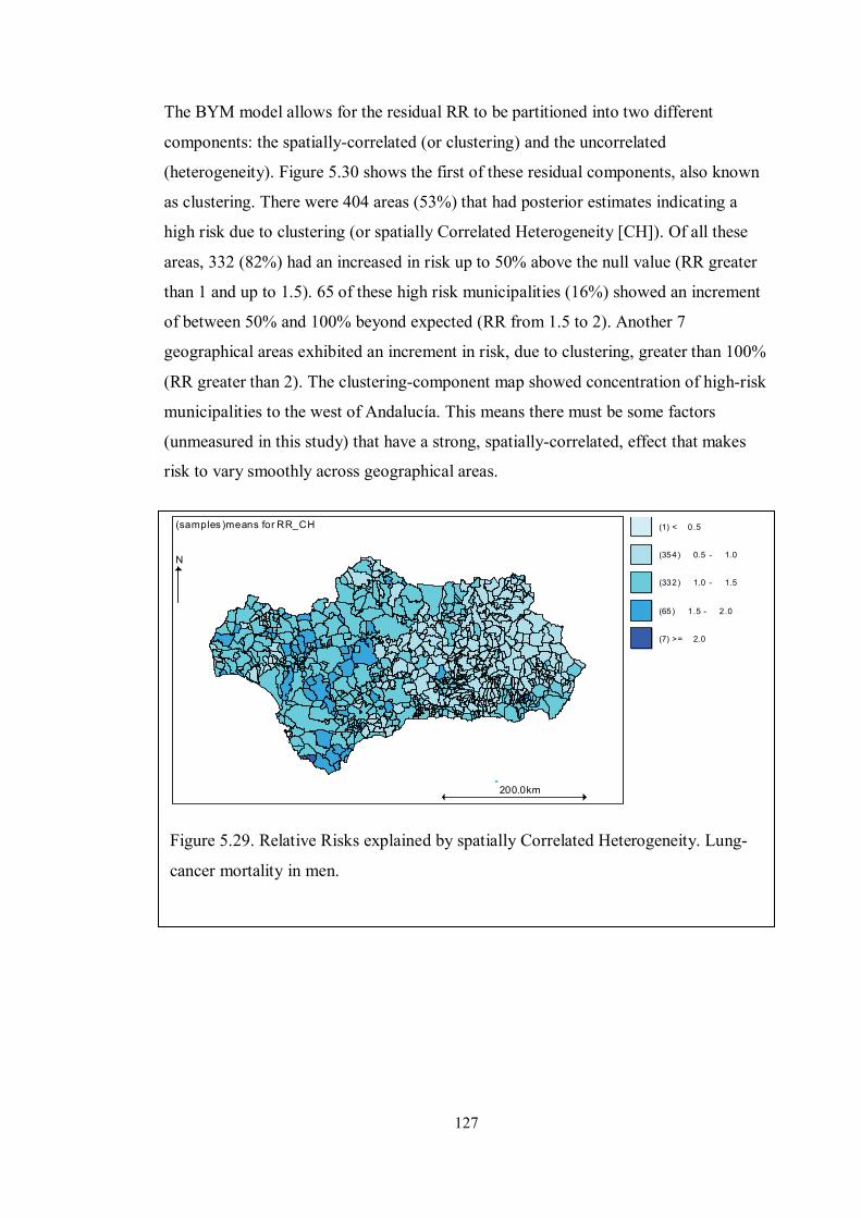
127

The BYM model allows for the residual RR to be partitioned into two different

components: the spatially-correlated (or clustering) and the uncorrelated

(heterogeneity). Figure 5.30 shows the first of these residual components, also known

as clustering. There were 404 areas (53%) that had posterior estimates indicating a

high risk due to clustering (or spatially Correlated Heterogeneity [CH]). Of all these

areas, 332 (82%) had an increased in risk up to 50% above the null value (RR greater

than 1 and up to 1.5). 65 of these high risk municipalities (16%) showed an increment

of between 50% and 100% beyond expected (RR from 1.5 to 2). Another 7

geographical areas exhibited an increment in risk, due to clustering, greater than 100%

(RR greater than 2). The clustering-component map showed concentration of high-risk

municipalities to the west of Andalucía. This means there must be some factors

(unmeasured in this study) that have a strong, spatially-correlated, effect that makes

risk to vary smoothly across geographical areas.



(1) < 0 .5

(354) 0.5 - 1.0

(332) 1.0 - 1.5

(65) 1 .5 - 2 .0

(7) >= 2.0

(samples )means for RR_CH

200.0km

N

128

To further assess the high and low-risk posterior estimates, Figure 5.31 and Figure

5.32 show the exceedance-probability maps. The former gives the probabilities of an

RR being greater than 1, while the latter shows the probabilities of an RR being less

than 1. It can be seen (Figure 5.31) that there were 115 municipalities (15%) for which

virtually all the area (at least 99%) under their respective RR curves were above the

value of 1 being, therefore, representative of high-risk values. Another 56 (7%)

municipalities had high probability (0.95 to 0.99, or 95% to 99%) of being

representative of high-risk zones. Again, the probabilities of finding high-risk

municipalities are greater to the west of Andalucía, as shown previously by the RR

map due to the clustering component.


Correlated Heterogeneity (Probability [Relative Risk > 1]). Lung-cancer mortality in

men.

(487) < 0.75

(43) 0 .75 - 0 .85

(58) 0 .85 - 0 .95

(56) 0 .95 - 0 .99

(115) >= 0 .99

probability of RR_CH greater than 1.0

200.0km

N

129

The opposite can be seen in Figure 5.32 where the probability of finding a low RR

(due to clustering) municipality was at least 0.99 (or 99%) for 63 of them out of 759

(or 8% of all the municipalities). While that probability varied from 0.95 to 0.99 (or

95% to 99%) for another 56 (7%) municipalities. Most of these high-probability low-

risk areas were concentrated to the east of Andalucía. These two complementary maps

show that the unmeasured factor (or factors) responsible for this spatial pattern seems

to operate to the west of the region.


Correlated Heterogeneity (Probability [Relative Risk < 1]). Lung-cancer mortality in

men.

(494) < 0.75

(48) 0 .75 - 0 .85

(99) 0 .85 - 0 .95

(55) 0 .95 - 0 .99

(63) >= 0.99

probability of RR_CH less than 1.0

200.0km

N

130

The second residual RR component, Uncorrelated Heterogeneity (UH) was mapped in

Figure 5.33, Figure 5.34, and Figure 5.35. Mapping of the RR due UH (or random

within-area variability) did not show a clear pattern, contrary to the one due to

clustering; that is to say, random noise is not responsible for this spatial pattern of

higher mortality to the west of the region. The maps show that 135 out of 759 areas

(18%) had an uncorrelated-RR of at least 1, and they were all scattered throughout the

region. Furthermore, only 2 municipalities showed a probability of being high-risk

areas, of 60% or greater (Figure 5.34) and 46 municipalities (6% of all geographical

areas) had a probability of at least 80% of being low-risk zones (Figure 5.35).

Figure 5.32. Relative Risks explained by Uncorrelated Heterogeneity. Lung-cancer

mortality in men.

(4) < 0 .85

(18) 0 .85 - 0 .9

(94) 0 .9 - 0 .95

(508) 0 .95 - 1.0

(135) >= 1 .0

(samples )means for RR_UH

200.0km

N

131

Figure 5.33 Exceedance-probabilities map for Relative Risks explained by

Uncorrelated Heterogeneity (Probability [Relative Risk > 1]). Lung-cancer mortality

in men.

(2) < 0 .0

(44) 0 .0 - 0 .2

(279) 0.2 - 0.4

(432) 0.4 - 0.6

(2) >= 0.6

probability of RR_UH greater than 1.0

200.0km

N

Figure 5.34. Exceedance-probabilities map for Relative Risks explained by

Uncorrelated Heterogeneity (Probability [Relative Risk < 1]). Lung-cancer mortality

in men.

(2) < 0 .4

(432) 0.4 - 0.6

(279) 0.6 - 0.8

(46) >= 0 .8

probability of RR_UH less than 1.0

200.0km

N

132

5.3.4 Mapping of lung-cancer mortality modelling: females

Similarly to the mapping implemented in section 5.3.3, the SMRs, before and after

modelling (in this case labelled as RRs), were mapped. Figure 5.36 presents the

SMRs, while Figure 5.37 shows the posterior RRs. It can be seen that while the SMRs

ranged from 0 to 8, the RRs were smoothed, the estimated values ranging only from 0

to 1.5, which is a characteristic inherent to multilevel models (such as the BYM

model). This smoothing effect was lower when fitting the males’ dataset (Figure 5.17

and Figure 5.18) as the RR estimates were based on a greater number of cases. This, in

turn, produced more reliable estimates which were not pulled down towards the

average value.

Figure 5.35. Standardised Mortality Ratios. Lung-cancer mortality in women.

(343) < 0 .0

(330) 0.0 - 2.0

(68) 2 .0 - 5 .0

(13) 5 .0 - 8 .0

(5) >= 8.0

(samples )means for SMR

200.0km

N

133

Figure 5.37 shows that only 80 municipalities out of 759 (or 10%) had a posterior RR

greater than 1. Most of these areas of high-risk mortality (75, or 95%) had up to a 25%

increment in risk. In contrast, 383 municipalities (or 50%) were classified as high risk

areas when the same BYM model was used to fit the males’ dataset (see 5.3.3 and

Figure 5.18). There is also a noticeable difference, between women and men, in the

magnitude of the risk: 323 of all high-risk areas (or 84%) showed up to a 50%

increment in risk. These results suggest a differential effect between men and women

of the explanatory variables included in the model. The spatial distribution of lung-

cancer mortality is also different for women; there is not a clear pattern of high-risk

areas concentrated to the west of the region (in contrast, see 5.3.3 for males’ results).

Figure 5.36. Posterior Relative Risks of lung-cancer mortality in women.

(103) < 0.75

(576) 0 .75 - 1.0

(75) 1 .0 - 1 .25

(4) 1.25 - 1 .5

(1) >= 1.5

(samples )means for RR

200.0km

N

134

The exceedance-probabilities map of an RR being greater than 1 helps identify those

municipalities likely to be high-risk areas. Figure 5.38 shows that the probability of an

RR being greater than 1 was lower than 0.75, for most of the areas (748 out of 759, or

99% of all municipalities). This means that, for these municipalities, less than 75% of

the area under their estimated probability-density curves was above the RR-value of 1.

Therefore low-risk values (lower than 1) are also likely (probability of 0.25).


cancer mortality in women.

(748) < 0.75

(3) 0.75 - 0 .85

(5) 0.85 - 0 .95

(0) 0.95 - 0 .99

(3) >= 0 .99

probability of RR greater than 1.0

200.0km

N

135



(238) < 0.75

(174) 0.75 - 0.85

(299) 0.85 - 0.95

(47) 0.95 - 0.99

(1) >= 0.99

probability of RR less than 1.0

200.0km

N

Figure 5.39 shows the exceedance-probabilities map of an RR being lower than 1.

This is a mirror image of Figure 5.38, which highlights probability of low-risk areas.

Thus, there are 299 areas (or 39%) for which the probability of being low-risk areas

ranged between 0.85 and 0.95. 47 areas (or 6%) were classified as low-risk areas with

probability between 0.95 and 0.99. Only 1 area had an estimated probability which

was, at least, 0.99.

136

Mapping of the clustering component for the women model (Figure 5.40) shows some

similarities with the model in men (Figure 5.30), as there seems to be a higher risk of

mortality, due to the clustering component, in the west (but also in the south) of

Andalucía.

5.4 Summary of lung-cancer mortality modelling

When compared to the model in section 5.2 (with just lithology and deprivation as

explanatory variables) model in section 5.3.1 was preferred based on different

functions. In this new model, there is also evidence of a positive association between

the lithology score and mortality due to lung cancer in men. Likewise, there exists a

positive association between deprivation and lung cancer mortality in men.

Additionally, the geographical variability in lung cancer mortality in men not captured

by either lithology or deprivation was also estimated. These estimates show that most

of the unexplained variance seems to be due to some factor (or factors), unmeasured in

this study, with a strong effect over neighbouring areas to the west of Andalucía.

Nevertheless, lithology is still shown to be an explanatory variable for lung-cancer

mortality in men.



(83) < 0.9

(230) 0.9 - 1.0

(429) 1.0 - 1.2

(16) 1 .2 - 1 .4

(1) >= 1.4

(samples )means for RR_CH

200.0km

N

137

Chapter 6. Discussion

6.1 Findings

The spatial distribution of lung-cancer deaths in Andalucía was found to be associated

with a lithology score, especially devised for this study as a surrogate measure for

potential radon-gas exposure. Furthermore, this association remained after adjusting

for area-level deprivation so that the potential confounding effect of tobacco smoking

was taken into account. These findings are in agreement with current scientific

knowledge: firstly, different epidemiological studies have consistently found an

association between lung cancer and radon-gas exposure [115, 189, 231], which is

known to be the second most important cause (after tobacco smoking [106]) of lung

cancer; secondly, presence of radon in the soil is known to depend on the bedrock

composition (e.g. there is high content of radon in granite [58, 61]), which explains the

high correlation that exists between radon content in the soil and lithology [61, 169,

170, 183, 190, 232, 233].

A positive (although weak) association was found, in this study, between the spatial

distribution of male lung-cancer deaths, across the Andalusian municipalities, and the

lithology score. This association was, on average, also positive for female lung-cancer

deaths; however, lack of such an association could not be excluded for women: the

posterior distribution for the estimate of the regression coefficient was scattered

around zero (see Figure 5.16). Some authors have hypothesised that the predominance

of distinct histological types in men (SCC) and women (adenocarcinoma) might be

explained by the exposure to different environmental factors: tobacco smoking and

radon-gas in men and women, respectively [16]. This hypothesis has been thought to

be supported by findings of a higher mortality rate due to lung cancer, in some cohorts

of women residing in northwest Spain. That is to say, those who were born before the

1940s (mostly non-smoking women) and resided in a predominantly granitic region [5,

16, 61, 165, 179, 180]. Nevertheless, there is epidemiological evidence of gender

susceptibility to tobacco smoke exposure [108]. This differential susceptibility has

been associated with higher levels of DNA adducts formation in women, which in

turn, is thought to be due to higher levels of female TSNs exposure. The number of

adenocarcinoma diagnoses increased in parallel with the female smoking prevalence

that, in Spain, started to reach epidemic proportions since the 1970s [234].

138

Additionally, it has been reported that major changes occurred in the tobacco

composition (such as manufacturing of filtered, as well as low-nicotine, cigarettes) at

that time. Hence, some researchers have attributed the responsibility for the

histological differences between male and female lung cancer, to these biological,

epidemiological, and manufacturing characteristics [107, 108].

Tobacco smoking is also thought to modify the effect of radon-gas exposure [114,

115]. From the statistical point of view, this interaction has been reported to have a

multiplicative (or nearly multiplicative) effect. This way, exposure to radon-gas would

entail a higher risk of lung-cancer development amongst smokers compared to non-

smokers. The way tobacco smoking modify the effect of radon-gas exposure is not

completely understood [116, 117]. However, several (non-exclusive) hypotheses exist:

radon-gas can penetrate the smaller airways by attaching to dust particles in the

ambient air; ventilation and deposition patterns differ between smokers and non-

smokers; the carcinogenic effect exerted by each exposure can eventually occur at

different, or similar, stages. Therefore, tobacco smoking and radon-gas can be

responsible for lung-cancer mortality by exerting their effect either independently

from each other, or synergistically. Consequently, it is important to take into account

both the potential confounding and interaction effects of tobacco smoking while

studying the association between lung-cancer mortality and lithology. Even though

direct information on tobacco smoking was not available, area-level deprivation was

used as a surrogate measure for tobacco smoking; this decision was based on reported

evidence about the association between smoking prevalence and area-level deprivation

[152, 156, 157]. It is important to note that in some instances [154], deprivation was

found to predict the smoking habit even after adjusting for individual-level SES.

In Spain, lower individual-level SES (as measured by educational level, or

occupational class) has been reported to be associated with higher rates of tobacco

smoking, as well as poorer self-perceived health status and higher prevalence of

chronic diseases [40]. Interestingly, measures of area-level deprivation were, overall,

reported to be in agreement with individual-level SES measures. The only exception

was for the association between female SES and the tobacco smoking habit. In this

case, lower individual-level SES was associated with lower prevalence of tobacco

smoking, while area-level deprivation was not associated with the smoking

prevalence. It is worth mentioning that the same area-level deprivation index and

139

census (the one from the year 1991) have been used in the present study. This

disagreement between individual-level SES and area-level deprivation measures

suggests that the latter may not be valid for adjusting on tobacco smoking, in this

female cohort. A study at the European level on a cohort recruited in the 1990s [32]

has confirmed the reverse association between female individual-level SES in Spain at

that time, and the smoking prevalence; however, no comparisons were made with

area-level deprivation in this instance.

Area-level deprivation is relevant in this context, not only because of its proven

association with measures of individual-level SES (with some exceptions [40]) which,

in turn, have been shown to be proxy measures for the prevalence of tobacco smoking,

as well as other health-related exposures. In addition, area-level deprivation has been

reported to be associated with radon-gas exposure [103]; interestingly, although

environmental pollution tends to be higher in most deprived areas, the association

between area-level deprivation and radon-gas exposure is the opposite way round:

least deprived areas are exposed the most to radon-gas (Figure 6.1). This inverse

association between deprivation and radon-gas has been explained by Briggs et al.

[103] by the fact that urban areas (which concentrate highly deprived zones) are

usually settled in lowland areas, where radon-gas concentration is lowest. In contrast,

high-altitude rural areas are both more exposed to radon-gas, and less deprived.

Therefore, area-level deprivation, as a surrogate measure for the prevalence of tobacco

smoking, can be used to check for the potential modifying effect (statistical

interaction) of smoking, on the association between lung cancer and radon-gas

exposure. Furthermore, adjusting for area-level deprivation (if interaction was not

present) is also important to controlling for the potential confounding effect of

deprivation on this same relationship between radon-gas exposure and lung-cancer

mortality. Notwithstanding the proven association between area-level deprivation and

both lung-cancer mortality and radon-gas exposure, it may be the case that the

deprivation index which was used, did not attain to reach a strong association with

either lung-cancer or radon-gas because of the individual components (percentage of

illiterate, unemployed, and unskilled workers) that comprises this index of deprivation.

Other possibilities exist and all have been reported to have a variable degree of

association depending on the outcome under consideration and the age groups that are

analysed [30].

140

Figure 6.1. Pathways in the association of deprivation with lung cancer and radon-gas.

= inverse association = direct association

(Both causal and non-causal associations are indicated by arrows)

= confounding = interaction

141

An alternative explanation for the absence of a clear association between lithology and

lung-cancer mortality in women can be based on two grounds: firstly, the modifying

effect of tobacco smoking on radon-gas exposure, as it has been reported that most

deaths due to radon-gas occur amongst smokers [115]; secondly, the prevalence of

smoking amongst women during the study period (1986-1995). Given that most

female deaths due to lung cancer took place in women aged 60 years and older, they

may mostly represent deaths of non-smoking women (the Spanish women born before

1940 did not have joined the tobacco-smoking habit yet). Consequently, a much

smaller risk (mean RR in women = 1.016 vs. mean RR in men = 1.023) may have

become undetectable due to the lack of statistical power (see 5.3.1 and Table 5.8, and

5.3.2 and Table 5.14): the same number of units of analysis (759 municipalities) were

used to detect a smaller RR [235]. Interaction (modelled as a multiplicative term

between area-level deprivation and the lithology scores) was not statistically

significant for either men or women. This can be explained by the fact that the area-

level deprivation is a proxy measure not only for tobacco smoking (at least in men) but

also for other various exposures; many of them may not modify the effect of radon-gas

exposure.

There is some research evidence that substantiates a small attributable risk due to

domestic radon-gas exposure in non-smoking women (1-4%), after 25 or more years

of exposure [236]. This was shown for a population of non-smoking women residing

in areas where the median radon-gas concentration was 4 pCi/L (or 150 Bq/m3): this

coincides with the threshold limit for which the US Environmental Protection Agency

(EPA) establishes the need to implement remedial actions. In contrast, some studies

have reported that the mean potential indoor radon-gas concentration in Andalucía is

around 25 Bq/m3. Nevertheless, it has also been reported that there exists some risk

even at lower levels than the limit set by the EPA. For instance, Darby et al. have

reported averaged estimates (from case-control studies) of RR = 1.06, for exposures to

doses around 100 Bq/m3 (95% confidence interval: 1.01-1.10) compared to non-

exposure. Also at concentrations of 20 Bq/m3 reported to be the average value in the

UK (lower than the mean estimated values in Andalucía), it was estimated to exist a

cumulative risk of lung-cancer death of 30% for smokers. This risk was only 0.8% for

non-smokers. The proportion of cases attributed to radon-gas exposure, alone, was

calculated to be 1% [115], which is in agreement with estimates reported by other

142

researches [189]. In the present study, the estimated magnitude of the average male

RR due to lithology (when comparing the highest vs. the lowest quintile of the

lithology score) was 1.07 (95% CI: 1.04-1.09).

Although extensively investigated, only lung-cancer has been associated with radon-

gas exposure, but no association has been established between other cancer sites and

radon [237, 238]. The findings in the present study are consistent with this. Tobacco

smoking is known to be the major risk factor for both COPD [100, 121, 131] and

larynx cancer [113, 239, 240]. In contrast, radon-gas exposure has not been related to

either of them [117, 238] (see 2.4.2 and 2.4.3 for COPD and larynx cancer,

respectively). Interestingly, the spatial distribution of male deaths due to either COPD,

or larynx cancer was not associated with the lithology score devised for this study (see

5.2.2). In contrast, all three diseases (lung cancer, COPD, and larynx cancer) were

positively associated with the area-level deprivation score; this is consistent with

current scientific knowledge concerning the association between lower SES and higher

rates of mortality due to all these diseases (see 2.4 and 2.5). These results point

towards a specific, plausible association between the spatial distribution of male lung-

cancer deaths in Andalucía, and the lithology score (as a surrogate measure for

potential radon-gas exposure).

However, some important factors remained unmeasured, as the residual variance

revealed. The individual estimation of the clustering and heterogeneity components

allowed the computation of the VPC (see Table 5.10 and Table 5.15). The VPC was

95% and 100% for the male and female models, respectively. This means that virtually

all the variance not explained by the models was due to the general clustering. This

component, which is spatially auto-correlated, is usually interpreted in terms of

unmeasured area-level factors that vary smoothly across the geographical areas; that is

to say, any particular area shares some (modelled) level of risk with its neighbouring

areas and differentiates from distant places.

Figure 5.30 and Figure 5.40 present the maps with the RRs due to the clustering

component for women and men, respectively. It can be observed that there is a pattern

of higher RRs of lung-cancer mortality (for both men and women) to the southwest of

Andalucía. This pattern of spatial variation in risk was not due to either lithology (or

not completely) or SES, but to some other unmeasured factor. Environmental factors

143

are frequently hypothesised to be responsible for this residual, spatially correlated,

variability.

Area-level deprivation is not only important as a surrogate measure for tobacco

smoking, but also because poorer health status has been consistently associated with

lower SES [142]. Furthermore, lung cancer incidence and mortality rates are higher

amongst people of lower SES even after adjusting for tobacco-smoking [32]. This is

due to the fact that SES can act as a proxy measure for many other lifestyle, as well as

environmental and work exposures (such as diet, physical activity, alcohol intake and

exposure to toxic substances). In this study, the spatial distribution of deaths due to all

three diseases (lung cancer, COPD, and larynx cancer) in both men and women has

been found to be positively associated with lower area-level deprivation. For lung

cancer, the mean estimated value of the RR due to area-level deprivation was 2%

higher than the RR due to lithology (1.04 vs. 1.02, Table 5.8); this is in agreement

with previous research that showed that the association between tobacco smoking and

SES was stronger for men than women [241].

6.2 Strengths and limitations

Small-area analysis is characterised by the small number of events under scrutiny

within the units of analysis. It is this characteristic that allows modelling of sparse data

by means of the Poisson distribution [235]. However, this theoretical probability

distribution is based on the strong assumption that the variance/mean ratio equals one.

If this premise does not hold due to the variance being greater than the mean,

overdispersion is said to exist. Three main overdispersion sources are unstructured (or

random) heterogeneity, spatially-correlated (or clustering) heterogeneity, and excess of

zeros in the data (due to the fact that this kind of analysis deals with rare events) [90].

Another strong premise when modelling the RRs is the proportionality assumption

[14, 99, 220, 235], which requires that the RRs in each stratum of the confounding

variable (e.g. age) be proportional to the corresponding strata in all the geographical

areas under study.

6.2.1 Bayesian analysis and modelling

Hierarchical Bayesian methods are well suited for the spatial analysis of

epidemiological data, as they allow the researcher to address these statistical issues

(see 6.2) [80]. Furthermore, Bayesian analysis offers some advantages over its

144

frequentist counterpart [79], such as incorporating prior knowledge into the analysis,

producing estimates with lower MSE than the frequentist ones, and allowing for a

direct interpretability of CIs, while a single postulate is used in any scenario: the

Bayes’ rule (see 4.2.2). Some of the modelling possibilities include the Poisson-

gamma, the log-normal and the BYM model; a further modification of the latter one,

by Waller, takes time into consideration. The Poisson-Gamma model is, from a

mathematical point of view, the simplest one. It models the observed number of cases

as Poisson distributed and considers the RR as a Gamma-distributed random effect

[63], which results in a Negative-Binomial posterior distribution [76, 242]. Although

mathematically convenient, as it addresses overdispersion (see 4.2.1), two main points

remain unresolved: covariate adjustment and spatiotemporal autocorrelation (or

clustering). Conversely, the log-normal model offers some advantages by modelling

the Poisson parameter on a log scale; this, allows for a linear combination of different

covariates to be included. A random component for the RR is included, which is

Gaussian distributed. This model can also accommodate a range of hierarchical

structures to analyse the spatiotemporal components of health-related events. One of

these hierarchical structures is implemented by means of the BYM which was used in

this study. This model splits the random component into CH and UH. The CH

component is, in turn, modelled by means of a CAR distribution (see 4.2), which

requires a definition of what neighbouring areas are to be considered, by means of the

adjacency matrix.

The way ‘neighbouring’ is defined (through the adjacency matrix) has been reported to

greatly affect the regression estimates. As a consequence, some researchers have

advocated a sensitivity analysis to take account of this issue [224]. These same

researchers showed the differences to be expected under distinct neighbourhood

structures. In all these settings, the comparative performance was assessed by means

of various common criteria. They took into consideration the degree of smoothness

attained as well as the magnitude of the clustering effect introduced; also, the effect on

the Deviance Information Criterion (DIC, see 4.2.2 ) which is used for model

selection. To quantify the agreement between observed and predicted values, the

Kappa index was used, a low-value being due to a high smoothing effect (see 4.2.2).

Interestingly, these researchers resorted to the Receiver Operating Characteristics

(ROC) curve to find the most appropriate predictive cutoff points; the aim was to

145

decide which one gives the best compromise between sensitivity and specificity; with

the same aim, other researchers have advocated fixed cut-off points based on

simulation studies (see 4.4).

The ROC curve analysis offers some advantages over the fixed cut-off point proposal:

firstly, it allows for the setting of cut-off points to be tailored to the actual data under

scrutiny; secondly, any predicted value across the whole variable range can be

assessed by means of the ROC curve. This is also advantageous, as different decision

rules (favouring either sensitivity or specificity) may be preferable under diverse

circumstances. The ROC curve is built by graphing the true positive ratio (sensitivity)

against the false negative ratio (1-specificity) [224, 225]; they are usually represented

on the y and x axis, respectively. To find these values, researchers studying modelling

performance under different neighbourhood definitions, cross tabulated observed and

predicted values [224]. Afterwards, they calculated the true positive and false negative

ratios within tertiles of the variable range. When the ROC curve is used to assess

modelling performance, the cut-off points defining the highest area under the curve are

preferred; this happens when the highest true-positive ratio and lowest false-negative

ratio co-occur. In this case, it was reported to happen under a predictive probability of

0.33; much different from the 0.7 cut-off point advised from simulation studies (see

4.4) [230] . The researchers concluded that neighbourhood structures based on

adjacencies (as in this study) produce the highest smoothing effect on the RR

estimates. Hence, they produce the least agreement between observed and predicted

values (kappa = 0.05). Conversely, distance-based models produce lower smoothing

and, therefore, higher agreement with observed values (kappa = 0.07). On the other

hand, adjacency-based neighbourhoods introduce the least amount of clustering, when

compared with distance-based models. They also determined that DIC reached the

highest values for adjacency matrices; this would make other structures (like distance-

based models) to be preferred, under this criterion.

Therefore, different possibilities (other than contiguity neighbours) exist, which can

be implemented. So, distance-based neighbours could also be devised; in this

approach, different lag distances (from their centroids) might be defined, as the

number of neighbours would increase with distance [224]. Also, adjacency matrices of

order higher than 1 (lists of neighbours of neighbours) can be considered; this was

shown to improve sensitivity from 77% to 78% and specificity from 41% to 43%,

146

when the first-order Queen-style model was compared with its second-order

counterpart. Distance-based models (or adjacency-based structures of order higher

than 1) may be important where some processes (like migration flows) are nested into

the weighting matrix; in this case, binary values would turn to different weights (e.g.

average of inflow/outflow migration rates). If such a tenet seems plausible, different

neighbouring definitions and weighting schemes should be tested in a sensitivity

analysis [224]. This is relevant when a CAR model is implemented, where differences

in neighbouring definitions and weighting schemes can be highly influential. This is

because they determine the smoothing rate, which is at the core of Bayesian

hierarchical modelling-techniques. Smoothing is designed to lessen random noise due

to the statistical instability inherent in the SMRs calculation. However, how much

smoothing is desirable constitutes a compromise between variance and bias.

As already discussed, the FB BYM model (that was used in this study) implements

smoothing by means of locally-varying weights; conversely, most EB methods use

global smoothers. There are some other important similarities (and differences)

between EB and FB methods. There is an EB version by Marshall, which uses local

smoothers, as the BYM model; the method devised by Marshall produces the least

shrinking effect when compared to other EB counterparts. Another similarity between

EB and FB methods is that some EB techniques fit the data through a log-normal

model; these EB models are considered to be the most statistically stable amongst its

class [62]. Despite all the affinities between these two kinds of Bayesian models, none

of the EB methods take into consideration inferential uncertainty (hyperprior-estimates

coming from the data itself). Hence, their RR estimates show less variability than

those produced by FB methods. This downside can also be considered advantageous,

due to the higher simplicity and quicker computation of EB methods.

In the present study, prior knowledge was incorporated into the analysis by fitting the

BYM model to male lung-cancer mortality data concerning the period 1981-1985. A

vague gamma hyperprior with parameters 0.5, 0.0005 was used to estimate both

components of the residual variance (CH and UH). The posterior estimates of these

two components were then used in the study of male lung-cancer mortality for the

period 1986-1995. In this second stage, a sensitivity analysis was done to assess the

effect of different hyperpriors on the RR estimates. The use of vague hyperpriors was

147

compared with the informed ones obtained in the previous step: there were not any

meaningful differences in the range of the RR estimates.

Further methods have more recently been proposed. These alternatives have arisen

from geostatistics, in view of the limitations of EB methods and complexity of FB

techniques; among the latter, the high shrinking effect of the BYM and subjectivity to

choose the adjacency matrix have encouraged new options. Some of these models

recently proposed rely on methods used to interpolate unknown values based on

known sample points (Kriging) [62, 77, 243-246]. Thus, Area-to-Area Poisson Kriging

has been claimed to outperform both EB and FB methods [246]. This superiority has

been grounded on modelling properties and practical results, as modelling through

Poisson Kriging can still produce a full posterior distribution, like FB models (under a

Gaussian assumption, this time). Results based on simulation studies have also shown

better discrimination between high-risk and low-risk RRs, for Poisson Kriging.

However, this depends on the sensitivity and specificity and which threshold values

are set by choosing different cutoff points.

An additional benefit of the Poisson Kriging method is that the characteristics and

effects of different adjacency matrices can be thoroughly described, which allows an

informed selection to be made. Also, smaller errors concerning both inferential and

predictive uncertainty have been reported, when compared to Bayesian methods [246].

Notwithstanding these findings, it is worthy of note that Area-to-Area Poisson Kriging

(as EB methods) does not address parameter uncertainty; this, in turn, provides with an

artifactual reassurance about the estimates precision, as all the information comes from

the data itself. All the arguments considered throughout this chapter contributed

turning to FB methods (specifically the BYM model) for the analysis stage.

A trade-off between sensitivity and specificity is always at issue where diagnostic

tools are used. This is also the case when the mapping process is meant to detect areas

of unusual high/low risk. As both characteristics counteract each other, the researcher

always has to decide to favour either sensitivity or specificity. In spatial analysis,

sensitivity refers to the ability of the mapping process (and the underlying model) to

detect true raised-risk areas. This is equivalent to the conditional probability of some

areas being classified as high-risk ones, given that its true risks are raised. Vice versa,

specificity names the capacity to detect true lowered-risk areas. Likewise, it is the

148

conditional probability of some areas being classified as low-risk ones, given that its

true risks are lowered. Most importantly, the researcher is interested about a different

set of conditional probabilities: the so called positive and negative predictive values.

Therefore, once the modelling stage has classified some areas as high-risk ones, the

probability of their true risks being raised is sought; this would be given by the

positive predictive value (PPV). The negative predictive value (NPV), would address

the opposite question: once the model has classified some areas as low-risk ones, the

probability of their true risks being lowered is of interest. These are the sort of

conditional probabilities that the modelling process addresses, through the estimates

obtained from the posterior distribution. Both sensitivity and specificity are mainly

inherent to the model itself, while the predictive capacity can vary under different

circumstances. So, the BYM model is known to produce over smoothing on both the

background and raised-risk areas, in general terms. This causes the model to have high

specificity and lower sensitivity, which may prevent from identifying small risks; such

a situation may be encountered where environmental risks are implicated in small-area

analysis [230], which is the case in this study.

Concerning predictive ability, the modelling performance may be affected by different

circumstances, such as the distribution of high-risk areas (either isolated or in clusters)

as well as the magnitude of the risk to be identified. Furthermore, for the same

magnitude of the RR, the number of cases expected may affect the predictive

performance (PPV and NPV); nevertheless, this affects the smoothed RRs in a much

lesser extent than the raw RRs. Therefore, the smoothed RRs are highly shrunk to the

value of 1 (under most conditions) for background (not raised-risk) areas. In contrast,

the raw RRs remain over-dispersed. It is also important to consider that all the above

characteristics (sensitivity/specificity and predictive values) are interrelated. This

interrelationship can be summarised as follows: high sensitivity leads to a high NPV

through a decrease in the number of false-negative results. Whereas high specificity

results in a high PPV by lessening the number of false-positive results [225].

Similarly, whenever sensitivity is set to a high value (by assuming a higher probability

of false positive results) specificity drops. And the reverse is also true; if high

specificity is sought (by assuming a higher probability of false-negative results)

sensitivity decreases.

149

To adjust sensitivity and specificity, some research based on simulation has addressed

the above issues to produce practical decision rules [230]. These decision rules are

meant to allow choosing the best compromise between sensitivity and specificity (RR

detection threshold) for a desired predictive value (or posterior probability cutoff

point). To select the most appropriate values, several loss functions were used where

false positive and false negative results were weighted using different rules [230]. The

aim was to find the smallest value for any particular loss function; all of it, within a

reasonable range of probabilities of detecting certain RR magnitude. An RR threshold

of 1 and a probability value of 0.80 were advocated when the CAR distribution (see

4.2.2) is applied. This was shown to be a decision rule with high specificity (around

97%), but lower sensitivity (around 71%). Keeping an RR threshold of 1 and changing

to a cutoff point of 0.7, sensitivity raised to 82%, while specificity dropped just to 94%

(under the assumption of a true RR of 1.65).

Another decision to be made, involves a common topic to any kind of map: how many

categories should be represented and which break points should be used. To address

this issue concerning class intervals, it is important to realise that different methods

can convey quite different information [62]. One method which is extensively used

consists of using quantiles (e.g. tertiles, quartiles or quintiles); the corresponding break

points can be used to partition the range of the cumulative distribution function of the

variable to represent. This method would distribute the number of observations evenly

in each class, across the whole range of the variable. Nevertheless, it is far from being

perfect; values of magnitude that are far apart from each other may be classified in the

same interval. This may happen as the only criterion used by the quantiles method is

the number of observations per class, rather than their magnitude. Although the

quantiles method may be useful to map uniform distributions, these are not usually

encountered in spatial analysis; more frequently, the risk surface is spatially

heterogeneous. Nevertheless, it may be acceptable where highly shrunk risks are

mapped, which is usually the case when the BYM model is used.

An alternative method is the equally spaced intervals (or absolute cut-points). This

technique (as well as the quantiles one) is supplied by GeoBUGS; in this case, the

range of the distribution is partitioned into class intervals of the same width; again,

this is appropriate to map variables that are uniformly distributed. In contrast, other

methods are meant to minimise the within class variance and maximise the between

150

class variance; it helps to label similar observations within the same class. Amongst

these, the Fisher-Jenks method uses this sort of ‘natural breaks’; this technique is

especially useful to map multimodal distributions. Another common method,

addresses variables that are Gaussian-like distributed; in this case, classes can be

devised to take into consideration dispersion from the mean value, in terms of

standard-deviation units.

151

Chapter 7. Conclusions

7.1 Summary

Results from the measurement part of a confirmatory SEM showed a positive

association between a spatially-correlated score variable and lithology (rock

composition) as a surrogate measure for potential radon-gas exposure (see 5.2.1); this

association was, as expected (see pg. 58), highest for plutonic and metamorphic rocks

(Table 5.1). The structural part of the SEM showed a positive association between the

lithology score, derived from the measurement part of the SEM, and the spatial

distribution of male lung-cancer deaths in Andalucía, for the period 1986-1995 (Table

5.2 and Figure 5.4). Moreover, this association remained after adjusting for area-level

deprivation, so that the potential confounding effect of deprivation [103], on the

association between lithology (as a surrogate measure for potential radon-gas

exposure) and the spatial distribution of lung-cancer mortality, was controlled for

(Table 5.7 and Table 5.8).

Lithology was also associated with the spatial distribution of female lung-cancer

deaths, although lack of such an association could not be completely excluded (Figure

5.16 and Table 5.14). A multiplicative interaction term between area-level deprivation

and lithology (as surrogate measures for tobacco smoking and potential radon-gas

exposure, respectively) was shown not to improve the goodness of fit of either the

male (see pg. 97) or the female model (see pg. 113). In contrast with the association

found between lithology and lung-cancer mortality in men, no association was found

between the lithology score and the spatial distribution of mortality due to either

larynx cancer or COPD (Table 5.2 and Figure 5.4). After adjusting for deprivation,

most of the residual (not captured by the model) variance, as measured by the VPC,

was due to spatial autocorrelation rather than random (non-spatial) heterogeneity

(Table 5.10 and Table 5.15). In contrast with lithology, deprivation was positively

associated with the spatial distribution of mortality due to all three diseases (lung

cancer, COPD and larynx cancer) in men (Figure 5.5, Table 5.7 and Table 5.8).

According to the DIC, the best model (in both men and women) was the one which

included not only lithology and deprivation, but also a clustering component (which

accounted for spatial autocorrelation), as well as a random-heterogeneity component

(Table 5.4 and Table 5.11). The full (all variables) model was also the one with least

152

predictive error, as shown by the results of the computed MSPE and MAPE (Table

5.5, Table 5.6, Table 5.12 and Table 5.13). The model accounting for spatial

autocorrelation attained a high smoothing effect on the SMR, while improving the

distinction between high and low-risk areas (Table 5.9). This, in turn, eased the

identification of high-risk municipalities. Even though the provinces of Cádiz (Figure

5.8) and Huelva (Figure 5.11) show the highest mean posterior RR (1.35 and 1.34,

respectively) there is ample heterogeneity amongst municipalities (Figure 5.7-Figure

5.14). At the other extreme, the provinces of Jaén (Figure 5.12) and Granada (Figure

5.10) show the lowest mean posterior RR (0.80 and 0.89, respectively).

Therefore, the well-known pattern [9, 10, 13, 16] of higher lung-cancer mortality in

western Andalucía, for the period 1986-1995 was confirmed (Figure 5.17-Figure

5.19). Mapping of the residual variance in men showed that the spatial variation in risk

was not completely explained by the model (Figure 5.27 and Figure 5.28).

Furthermore, the residual variance was mainly due to the clustering component

(Figure 5.30 and Figure 5.31), which is the sort of influences that have been linked to

the so called contextual variables [98, 152, 156, 230]; in contrast, the random-

heterogeneity component did not show any visual patterning (Figure 5.33 and Figure

5.34). Notwithstanding these results, lithology can partially explain the spatial

distribution of lung-cancer mortality in Andalucía (Figure 5.21-Figure 5.23),

especially in men. Differences were found between men and women, in the effect of

the clustering component on the spatial distribution of lung-cancer mortality. A clear

pattern of higher risk in western Andalucía was seen in men (Figure 5.30 and Figure

5.31), while in women there was also higher risk to the south (Figure 5.40).

7.2 Contribution

This is the first time that the spatial distribution of potential radon-gas exposure from

the Andalusian soils has been comprehensively analysed without the aid of direct

radon measurements. Previous research had mainly relied on the availability of radon-

gas measurements for the design of risk maps by large areas [58, 61, 165, 179, 180].

Surrogate measures for radon-gas concentration had been only used when missing

values for actual measurements had to be confronted [61]. Although there has been

extensive research on the correlation between both geology and surface lithology, and

potential radon-gas exposure [168, 169, 171, 192] modelling of radon-gas

153

concentration as a latent (unobservable) variable (see 4.4.2 and 5.2.1) had not been

previously accomplished. The SEM approach to modelling had been already applied to

research on health related outcomes [195-197], but not to the analysis of the

association between lithology and lung-cancer mortality at the small-area level (see

5.2.2).

The present study has explored a novel lithology score which can partially explain the

spatial distribution of lung-cancer deaths in Andalucía. Lithology, as a surrogate

measure for potential radon-gas exposure, overcomes some difficulties inherent in the

actual measurement of radon-gas concentration. One such difficulties is the cost of

measurements that limits the number of sampled places [165]; also, lack of

measurements reliability due to spatial and seasonal variation in radon levels [116,

166, 173], as well as differing patterns of behaviour styles of the people dwelling in

the buildings [58]. In contrast a wealth of lithological information, of a high resolution

level, is available at no cost for the Andalusian soils [60]. FB methods are well suited

for the analysis of small RR due to environmental pollutants [1, 103], such as the one

posed by radon-gas exposure [115]; this is especially the case in Andalucía, where the

mean levels of radon-gas concentration are low [61]. The model developed in this

study has the potential for future improvement, so that it helps to guide public health

policy concerning potential radon-gas exposure in Andalucía; one key advantage is the

possibility to individually identify high-risk areas (Figure 5.7 and Figure 5.14). In

addition, this model can identify areas according to the risk which is solely due to

potential radon-gas exposure (Table 5.7, Table 5.8, Figure 5.21 and Figure 5.22),

which can be useful to prioritising municipalities where direct radon measurements

should be implemented, so that remediation actions be taken where needed [176].

7.3 Future research

The lithology score devised in this study (section 5.2) can be further elaborated in

different directions. Given that there is availability of comprehensive information on

the lithology of the Andalusian soils (see pg. 56 and Figure 3.1)[60], the SEM can be

used to explore different measurement approaches to accounting for the latent variable

(potential radon-gas exposure). Thus, extension of geological faults or different

lithological classes can be used [58, 61] for a better ascertainment of the latent

variable; simultaneously alternatives to the CAR model that was used to derive the

154

lithology score (section 5.2.1) can be checked by exploring model sensitivity to

different definitions of the adjacency matrix other than contiguity (see pg. 69); this

way, proximity, concentration, or intensity, concerning the latent variable (presence of

radon-gas), could be better captured [103].

Given that the area-level deprivation has been shown to be inversely associated with

radon-gas exposure [103], as well as (in a variable way) with lung-cancer mortality, it

seems appropriate to investigate the potential confounding effect of other choices of

deprivation indices (see pg. 4). Therefore, instead of using the so called index I

(illiteracy, unemployment, unskilled work), index II (illiteracy, unemployment, house

overcrowding) could be adjusted for [30]. As the chances are that neither index I or II

be associated with smoking in the women’s cohort that was analysed (section 6.1)

[40], a different surrogate measure for tobacco smoking should be used to test for the

potential interaction effect between lithology and smoking (Figure 6.1). An interesting

variable to use as a surrogate measure for tobacco smoking is COPD incidence, given

that this condition is mainly caused by tobacco smoke (section 2.4.2). Because of the

very poor survivorship of lung cancer patients (see pg. 5), there may not be a great

difference between modelling either lung-cancer incidence or mortality. In contrast,

COPD is characterised by a much better prognosis (section 2.4.2) that can make it

difficult distinguish between aetiological and prognostic factors, which, in turn would

produce biased results. In addition, using information concerning histological types

could also help to checking the hypothesis that different histological types (SCLC in

men and mainly adenocarcinoma in women) are due to distinct aetiological causes,

namely tobacco-smoking in men and radon-gas exposure in women [16]. Last but not

least, smaller geographical areas can be used to lessen the potential bias due to the

ecological fallacy. To this aim, digital boundaries at the census tract level are readily

available [27, 28].

155

Chapter 8. References 1. Elliott, P. and Wartenberg, D., Spatial epidemiology: current approaches and

future challenges. Environ Health Perspect, 2004. 112(9): p. 998-1006.

2. Lopez-Abente Ortega, G., Gervas Camacho, J.J., and Errazola Saizar, M.,

Analysis of geographic differences in mortality in Spain. Med Clin (Barc),

1985. 84(7): p. 264-7.

3. Vioque, J. and Bolumar, F., Trends in mortality from lung cancer in Spain,

1951-80. J Epidemiol Community Health, 1987. 41(1): p. 74-8.

4. Errezola, M., Lopez-Abente, G., and Escolar, A., Geographical patterns of

cancer mortality in Spain. Recent Results Cancer Res, 1989. 114: p. 154-62.

5. López-Abente, G., Pollán, M., and Jiménez, M., Female Mortality Trends in

Spain Due to Tumors Associated with Tobacco Smoking. Cancer Causes &

Control, 1993. 4(6): p. 539-45.

6. Barrado Lanzarote, M.J., Medrano Albero, M.J., and Almazan Isla, J.,

Mortality from ischemic cardiopathy in Spain: the trends and geographic

distribution. Rev Esp Cardiol, 1995. 48(2): p. 106-14.

7. Benach, J. and Yasui, Y., Geographical patterns of excess mortality in Spain

explained by two indices of deprivation. J Epidemiol Community Health, 1999.

53(7): p. 423-31.

8. Olalla, M.T., et al., Time trends, cohort effect and spatial distribution of

cerebrovascular disease mortality in Spain. Eur J Epidemiol, 1999. 15(4): p.

331-9.

9. Lopez-Abente Ortega, G., et al., Atlas of cancer mortality and other causes of

death in Spain 1978-1992. 2001, Ministerio de Sanidad y Consumo. Instituto

de Salud Carlos III: Madrid.

10. Benach, J., Geografia de la salud: el suroeste español bajo el microscopio.

Revista de Calidad Asistencial, 2002. 17(6): p. 317-18.

11. Benach, J., et al., Examining geographic patterns of mortality: the atlas of

mortality in small areas in Spain (1987-1995). Eur J Public Health, 2003.

13(2): p. 115-23.

12. Boix Martinez, R., Aragones Sanz, N., and Medrano Albero, M.J., Trends in

mortality from ischemic heart disease in 50 Spanish provinces. Rev Esp

Cardiol, 2003. 56(9): p. 850-6.

156

13. Benach, J., et al., The geography of the highest mortality areas in Spain: a

striking cluster in the southwestern region of the country. Occup Environ Med,

2004. 61(3): p. 280-1.

14. Ferrandiz, J., et al., Spatial analysis of the relationship between mortality from

cardiovascular and cerebrovascular disease and drinking water hardness.

Environ Health Perspect, 2004. 112(9): p. 1037-44.

15. Ocana-Riola, R., et al., Research protocol for the mortality atlas of the

provincial capitals of Andalusia and Catalonia (AMCAC Project). Rev Esp

Salud Publica, 2005. 79(6): p. 613-20.

16. Lopez-Abente Ortega, G., et al., Municipal Atlas of Cancer Mortality in Spain,

1989-1998, Carlos III Health Institute, Editor. 2006.

17. Spanish National Statistics Institute. Estimate of the Municipal Register at 1

January 2009. Provisional data. [Web] 2009 [cited 30/03/2012]; Available

from: http://www.ine.es/en/prensa/np551_en.pdf.

18. Consejería de Medio Ambiente. Datos Basicos de Medio Ambiente en

Andalucia. [Web] 2008 [cited 30/03/2012]; Available from:

http://www.juntadeandalucia.es/medioambiente/site/web/menuitem.a5664a214

f73c3df81d8899661525ea0/?vgnextoid=4b2a6b2464f4e110VgnVCM1000001

325e50aRCRD&vgnextchannel=f40a776da8e5e110VgnVCM1000001325e50a

RCRD&lr=lang_es.

19. Quantum GIS development team. Quantum GIS Geographic Information

System. Open Source Geospatial Foundation Project. [Web] [cited

30/03/2012]; Available from: http://qgis.org/.

20. Patterson, T. and Vaughn Kelso, N. Natural Earth. [Web] [cited 30/03/2012];

Available from: http://www.naturalearthdata.com/.

21. Instituto Nacional de Estadística (INE). INEbase. List of place names.

Methodology. [Web] [cited 05/04/2012]; Available from:

http://www.ine.es/nomen2/Metodologia.do?L=1.

22. Instituto de Estadística de Andalucía (IEA). Catalogue of Entities and

Population Centres. Andalusia. [Web] [cited 05/04/2012]; Available from:

http://www.juntadeandalucia.es/institutodeestadistica/nomenclator/index-

en.htm.

http://www.ine.es/en/prensa/np551_en.pdf�

http://www.juntadeandalucia.es/medioambiente/site/web/menuitem.a5664a214f73c3df81d8899661525ea0/?vgnextoid=4b2a6b2464f4e110VgnVCM1000001325e50aRCRD&vgnextchannel=f40a776da8e5e110VgnVCM1000001325e50aRCRD&lr=lang_es�




http://qgis.org/�

http://www.naturalearthdata.com/�

http://www.ine.es/nomen2/Metodologia.do?L=1�

http://www.juntadeandalucia.es/institutodeestadistica/nomenclator/index-en.htm�

http://www.juntadeandalucia.es/institutodeestadistica/nomenclator/index-en.htm�

157

23. Consejeria de Salud. Estadísticas vitales: Evolución de la mortalidad en

Andalucía de 1975 a 1997 [Web] 1999 [cited 30/03/2012]; Available from:

http://www2.uca.es/hospital/EV7597/index.htm.

24. Kogevinas, M., et al., Social Inequalities and Cancer, in IARC Scientific

Publication No. 138, N.P. M. Kogevinas, M. Susser and P. Boffetta, Editor.

1997, International Agency for Research on Cancer, Lyon,.

25. Dominguez-Berjon, M.F. and Borrell, C., Mortalidad y privación

socioeconómica en las secciones censales y los distritos de Barcelona. Gac

Sanit, 2005. 19(5): p. 363-9.

26. Ruiz-Ramos, M., et al., Evolución de las desigualdades sociales en la

mortalidad general de la ciudad de Sevilla (1994-2002). Gac Sanit, 2006.

20(4): p. 303-10.

27. Ocana-Riola, R., et al., Mortality Atlas of the provincial capitals of Andalucia,

1999-2002., ed. R. ocana Riola. 2007, Granada: Escuela Andaluza de Salud

Publica. Consejeria de Salud. Junta de Andalucia.

28. Ocana-Riola, R., et al., Area deprivation and mortality in the provincial capital

cities of Andalusia and Catalonia (Spain). J Epidemiol Community Health,

2008. 62(2): p. 147-52.

29. Benach, J., et al., The public health burden of material deprivation: excess

mortality in leading causes of death in Spain. Preventive Medicine, 2003.

36(3): p. 300-8.

30. Benach, J., et al., Material deprivation and leading causes of death by gender:

evidence from a nationwide small area study. J Epidemiol Community Health,

2001. 55(4): p. 239-45.

31. Tomatis, L., Poverty and cancer, in Social Inequalities and Cancer, M.

Kogevinas, et al., Editors. 1997, International Agency for Research on Cancer

(IARC): Lyon.

32. Menvielle, G., et al., The Role of Smoking and Diet in Explaining Educational

Inequalities in Lung Cancer Incidence. J. Natl. Cancer Inst., 2009. 101(5): p.

321-30.

33. International Epidemiological Association (IEA), The development of modern

Epidemiology: Personal reports of those who were there 1st ed, ed. W. Walter,

J. Olsen, and C.d.V. Florey. 2007, Oxford: Oxford University Press. 456 pp.

http://www2.uca.es/hospital/EV7597/index.htm�

158

34. Elliott, P., Investigation of disease risks in small areas. Occup Environ Med,

1995. 52(12): p. 785-9.

35. Salmond, C. and Crampton, P., Heterogeneity of deprivation within very small

areas. Journal of Epidemiology and Community Health, 2002. 56(9): p. 669-

70.

36. McNally, R.J. and Eden, T.O., An infectious aetiology for childhood acute

leukaemia: a review of the evidence. Br J Haematol, 2004. 127(3): p. 243-63.

37. Borrell, C. and Pasarin, M.I., Desigualdades en salud y territorio urbano. Gac

Sanit, 2004. 18(1): p. 1-4.

38. Ahs, A.M. and Westerling, R., Mortality in relation to employment status

during different levels of unemployment. Scand J Public Health, 2006. 34(2): p.

159-67.

39. Banks, J., et al., Disease and disadvantage in the United States and in

England. JAMA, 2006. 295(17): p. 2037-45.

40. Dominguez-Berjon, F., et al., The usefulness of area-based socioeconomic

measures to monitor social inequalities in health in Southern Europe. Eur J

Public Health, 2006. 16(1): p. 54-61.

41. Poole, C., et al., Socioeconomic status and childhood leukaemia: a review. Int.

J. Epidemiol., 2006. 35(2): p. 370-84.

42. Manda, S., Feltbower, R., and Gilthorpe, M., Investigating spatio-temporal

similarities in the epidemiology of childhood leukaemia and diabetes. Eur J

Epidemiol, 2009. 24(12): p. 743-52.

43. MacNab, Y.C. and Dean, C.B., Spatio-temporal modelling of rates for the

construction of disease maps. Stat Med, 2002. 21(3): p. 347-58.

44. Agarwal, D.K., Gelfand, A.E., and Citron-Pousty, S., Zero-inflated models

with application to spatial count data. Environmental and Ecological Statistics,

2002. 9(4): p. 341-55.

45. Silva Ayçaguer, L., Análisis espacial de la mortalidad en áreas geográficas

pequeñas. El enfoque bayesiano. Rev Cubana Salud Pública, 2003. 29(4): p.

314-22.

46. Kaminska, I.A., Oldak, A., and Turski, W.A., Geographical Information

System (GIS) as a tool for monitoring and analysing pesticide pollution and its

impact on public health. Ann Agric Environ Med, 2004. 11(2): p. 181-4.

159

47. Nakaya, T., et al., Geographically weighted Poisson regression for disease

association mapping. Statistics in Medicine, 2005. 24(17): p. 2695-717.

48. Ugarte, M.D., Ibáñez, B., and Militino, A.F., Detection of spatial variation in

risk when using CAR models for smoothing relative risks. Stoch Environ Res

Risk Assess, 2005. 19(1): p. 33-40.

49. Kraak, M.J., Why maps matter in GIScience. Cartographic Journal, 2006.

43(1): p. 82-9.

50. Bivand, R., Implementing Spatial Data Analysis Software Tools in R.

Geographical Analysis, 2006. 38(1): p. 23-40.

51. Martinez-Martinez, J.M., Statistical Applications in Geographical Health

Studies. 2006, Universitat Politècnica de Catalunya: Barcelona.

52. Greenland, S., Bayesian perspectives for epidemiological research: I.

Foundations and basic methods. Int. J. Epidemiol., 2006. 35(3): p. 765-75.

53. Reibel, M., Geographic Information Systems and Spatial Data Processing in

Demography: a Review. Popul Res Policy Rev, 2007. 26(5): p. 601-18.

54. Greenland, S., Bayesian perspectives for epidemiological research. II.

Regression analysis. Int. J. Epidemiol., 2007. 36(1): p. 195-202.

55. Elliott, P., et al., The Small Area Health Statistics Unit: a national facility for

investigating health around point sources of environmental pollution in the

United Kingdom. J Epidemiol Community Health, 1992. 46(4): p. 345-9.

56. Singh, G.K. and Hiatt, R.A., Trends and disparities in socioeconomic and

behavioural characteristics, life expectancy, and cause-specific mortality of

native-born and foreign-born populations in the United States, 1979-2003. Int.

J. Epidemiol., 2006. 35(4): p. 903-19.

57. Laflamme, D.M. and Vanderslice, J.A., Using the Behavioral Risk Factor

Surveillance System (BRFSS) for exposure tracking: experiences from

Washington State. Environ Health Perspect, 2004. 112(14): p. 1428-33.

58. Lopez, R., et al., Natural radiation doses to the population in a granitic region

in Spain. Radiat Prot Dosimetry, 2004. 111(1): p. 83-8.

59. Garcia-Perez, J., et al., Description of industrial pollution in Spain. BMC

Public Health, 2007. 7(1): p. 1-13.

60. Consejería de Medio Ambiente. Mapa litológico de Andalucía [Andalusian

lithological map]. [Web] 2005 [cited 29/04/2012]; Lithological map of

Andalucia, based on the Spanish National Geologic Map -MAGNA-, and the

160

Geologic and Miner Map of Andalucia. Scale 1:400,000]. Available from:

http://www.juntadeandalucia.es/medioambiente/site/rediam/menuitem.04dc442

81e5d53cf8ca78ca731525ea0/?vgnextoid=3097d2aa40504210VgnVCM10000

01325e50aRCRD&vgnextchannel=7b3ba7215670f210VgnVCM1000001325e

50aRCRD&vgnextfmt=rediam&lr=lang_es.

61. Quindos Poncela, L.S., et al., Natural gamma radiation map (MARNA) and

indoor radon levels in Spain. Environ Int, 2004. 29(8): p. 1091-6.

62. Bivand, R.S., Pebesma, E.J., and Gomez-Rubio, V., Applied Spatial Data

Analysis with R. Use R!, ed. R. Gentleman, G. Parmigiani, and K. Hornik.

2008, New York: Springer.

63. Lawson, A.B., Browne, W.J., and Vidal-Rodeiro, C.L., Disease Mapping with

WinBUGS and MLwiN, in Statistics in Practice, S. Senn and V. Barnett,

Editors. 2003, John Wiley & Sons: Chichester.

64. Dolk, H., et al., A standardisation approach to the control of socioeconomic

confounding in small area studies of environment and health. J Epidemiol

Community Health, 1995. 49 Suppl 2: p. S9-14.

65. Bithell, J.F., et al., Controlling for socioeconomic confounding using

regression methods. J Epidemiol Community Health, 1995. 49(Suppl_2): p.

S15-19.

66. Kogevinas, M. and Porta, M., Socioeconomic differences in cancer survival: a

review of the evidence, in Social Inequalities and Cancer, M. kogevinas, et al.,

Editors. 1997, International Agency for Research on Cancer (IARC). p. 177-

206.

67. World Health Organization. International Statistical Classification of Diseases

and Related Health Problems. 10th Revision. Version for 2007. [Web] [cited

05/04/2012]; Available from: http://www.who.int/classifications/icd/en/.

68. Benavides, F.G., Bolumar, F., and Peris, R., Quality of Death Certificates in

Valencia, Spain. American Journal of Public Health, 1989. 79(10): p. 1352-4.

69. Perez-Gomez, B., et al., Accuracy of cancer death certificates in Spain: a

summary of available information. Gac Sanit, 2006. 20 Suppl 3: p. 42-51.

70. Mantel, N. and Stark, C.R., Computation of Indirect-Adjusted Rates in the

Presence of Confounding. Biometrics, 1968. 24(4): p. 997-1005.

http://www.juntadeandalucia.es/medioambiente/site/rediam/menuitem.04dc44281e5d53cf8ca78ca731525ea0/?vgnextoid=3097d2aa40504210VgnVCM1000001325e50aRCRD&vgnextchannel=7b3ba7215670f210VgnVCM1000001325e50aRCRD&vgnextfmt=rediam&lr=lang_es�




http://www.who.int/classifications/icd/en/�

161

71. Breslow, N. and Day, N., Indirect Standardization and Multiplicative Models

for Rates, With Reference to the Age Adjustment of Cancer Incidence and

Relative Frequency Data. J Chronic Dis, 1975. 28: p. 289-303.

72. Osborn, J., A Multiplicative Model for the Analysis of Vital Statistics Rates.

Applied Statistics, 1975. 24(1): p. 75-84.

73. Clayton, D. and Kaldor, J., Empirical Bayes Estimates of Age-Standardized

Relative Risks for Use in Disease Mapping. Biometrics, 1987. 43(3): p. 671-

681.

74. Armstrong, B.G., Comparing standardized mortality ratios. AEP, 1995. 5(1):

p. 60-4.

75. Lee, W.-C., A Partial SMR Approach to Smoothing Age-specific Rates. AEP,

2003. 13(2): p. 89-99.

76. Bolstad, W.M., Introduction to Bayesian Statistics. 2nd ed. 2007: Wiley.

77. Crawley, J.M., The R Book. 2007, Chichester: Wiley.

78. Gelman, A. and Hill, J., Data Analysis Using Regression and

Multilevel/Hierarchical Models. 2007, Cambridge: Cambridge University

Press.

79. Dunson, D.B., Commentary: practical advantages of Bayesian analysis of

epidemiologic data. Am J Epidemiol, 2001. 153(12): p. 1222-6.

80. Graham, P., Intelligent smoothing using hierarchical bayesian models.

Epidemiology, 2008. 19(3): p. 493-5.

81. Ioannidis, J.P.A., Why Most Published Research Findings Are False. PLoS

Med, 2005. 2(8): p. 696-701.

82. Greenland, S., Principles of multilevel modelling. Int. J. Epidemiol., 2000.

29(1): p. 158-67.

83. Feltbower, R.G., et al., Detecting small-area similarities in the epidemiology of

childhood acute lymphoblastic leukemia and diabetes mellitus, type 1: a

Bayesian approach. Am J Epidemiol, 2005. 161(12): p. 1168-80.

84. National Center for Biotechnology Information. U.S. National Library of

Medicine. PubMed. [Web] [cited 27/06/2012]; Available from:

http://www.ncbi.nlm.nih.gov/pubmed.

85. Consejeria de Salud. Estadísticales vitales: Distribución espacial y tendencia

de la mortalidad por cáncer y otras causas. Andalucía, 1975-1997. 1998

http://www.ncbi.nlm.nih.gov/pubmed�

162

[cited 05/04/2012]; Available from:

http://www2.uca.es/hospital/AtlasAnda/indice.htm.

86. Consejeria de Salud. Estadísticas Vitales 1992-2003. Datos Andalucía y

Provincias Statistics [PDF files] 2003 [cited Sep 152009]; Available from:

http://www.juntadeandalucia.es/institutodeestadistica/ema/index.htm.

87. Doll, R. and Hill, A.B., Smoking and carcinoma of the lung; preliminary

report. BMJ, 1950. 2(4682): p. 739-48.

88. Clayton, D.G., Bernardinelli, L., and Montomoli, C., Spatial correlation in

ecological analysis. Int J Epidemiol, 1993. 22(6): p. 1193-202.

89. Thonsom Reuters. EndNote. [Web] [cited 27/06/2012]; Available from:

http://www.endnote.com/.

90. Ugarte, M.D., Ibanez, B., and Militino, A.F., Modelling risks in disease

mapping. Stat Methods Med Res, 2006. 15(1): p. 21-35.

91. Ramis Prieto, R., et al., Modelling of municipal mortality due to

haematological neoplasias in Spain. J Epidemiol Community Health, 2007.

61(2): p. 165-71.

92. Lawson, A.B., et al., Disease mapping models: an empirical evaluation. Statist

Med, 2000. 19(17-18): p. 2217-41.

93. Ghosh, S.K., Mukhopadhyay, P., and Lu, J.-C. (2006) Bayesian analysis of

zero-inflated regression models. Journal of Statistical Planning and Inference

136, 1360-1375.

94. Lawson, A.B. and Clark, A. (2002) Spatial mixture relative risk models

applied to disease mapping. Statistics in Medicine 21, 359-370.

95. Aragones, N., et al., Oesophageal cancer mortality in Spain: a spatial analysis.

BMC Cancer, 2007. 7: p. 1-13.

96. Ocana-Riola, R. and Maria Mayoral-Cortes, J., Spatio-temporal trends of

mortality in small areas of Southern Spain. BMC Public Health, 2010. 10.

97. Lopez-Abente Ortega, G., Aragones, N., and Pollan, M., Solid-tumor mortality

in the vicinity of uranium cycle facilities and nuclear power plants in Spain.

Environ Health Perspect, 2001. 109(7): p. 721-9.

98. Lopez-Abente Ortega, G., et al., Geographical pattern of brain cancer

incidence in the Navarre and Basque Country regions of Spain. Occup Environ

Med, 2003. 60(7): p. 504-8.

http://www2.uca.es/hospital/AtlasAnda/indice.htm�

http://www.juntadeandalucia.es/institutodeestadistica/ema/index.htm�

http://www.endnote.com/�

163

99. Ferrándiz, J., et al., Statistical relationship between hardness of drinking water

and cerebrovascular mortality in Valencia: a comparison of spatiotemporal

models. Environmetrics, 2003. 14(5): p. 491-510.

100. Viegi, G., et al., Definition, epidemiology and natural history of COPD. Eur

Respir J, 2007. 30(5): p. 993-1013.

101. Escolar-Pujolar, A. Atlas de mortalidad por cancer en la provincia de Cádiz

(1975-1979). XIII congreso de la Sociedad Española de Salud Pública y

Administración Sanitaria [Conference] 2009 [cited 05/04/2012]; Available

from: http://www.sespas.es/congresosevilla2009/ponencias.html.

102. Shohaimi, S., et al., Residential area deprivation predicts smoking habit

independently of individual educational level and occupational social class. A

cross sectional study in the Norfolk cohort of the European Investigation into

Cancer (EPIC-Norfolk). J Epidemiol Community Health, 2003. 57(4): p. 270-

6.

103. Briggs, D., Abellan, J.J., and Fecht, D., Environmental inequity in England:

small area associations between socio-economic status and environmental

pollution. Soc Sci Med, 2008. 67(10): p. 1612-29.

104. Woodward, A. and Boffetta, P., Environmental exposure, social class, and

cancer risk, in Social Inequalities and Cancer, M. kogevinas, et al., Editors.

1997, International Agency for Research on cancer (IARC). p. 361-7.

105. Doll, R., et al., Mortality in relation to smoking: 50 years' observations on

male British doctors. BMJ, 2004. 328(7455): p. 1519.

106. Doll, R., et al., Mortality from cancer in relation to smoking: 50 years

observations on British doctors. Br J Cancer, 2005. 92(3): p. 426-9.

107. Shields, P.G., Molecular epidemiology of smoking and lung cancer. Oncogene,

2002. 21(45): p. 6870-6.

108. Shields, P.G., Epidemiology of tobacco carcinogenesis. Curr Oncol Rep, 2000.

2(3): p. 257-62.

109. Alberg, A.J. and Samet, J.M., Epidemiology of lung cancer. Chest, 2003.

123(0732-183X (Print)): p. 21S-49S.

110. Sasco, A.J., Secretan, M.B., and Straif, K., Tobacco smoking and cancer: a

brief review of recent epidemiological evidence. Lung Cancer, 2004. 45 Suppl

2: p. S3-9.

http://www.sespas.es/congresosevilla2009/ponencias.html�

164

111. Boyle, P., Tobacco smoking and the British doctors' cohort. Br J Cancer, 2005.

92(3): p. 419-20.

112. IARC, I.A.f.R.o.C., Tobacco Smoking and Tobacco Smoke in IARC

Monographs on the Evaluation of Carcinogenic Risks to Humans and their

Supplements: A complete list. 2002.

113. Kuper, H., Adami, H.O., and Boffetta, P., Tobacco use, cancer causation and

public health impact. J Intern Med, 2002. 251(6): p. 455-66.

114. Alavanja, M.C.R., et al., Estimating the attributable risk of residential radon

among nonsmoking women: initial results and methodologic challenges.

Environ Int, 1996. 22(1001): p. 1005-13.

115. Darby, S., Hill, D., and Doll, R., Radon: A likely carcinogen at all exposures.

Ann Oncol, 2001. 12(10): p. 1341-51.

116. ATSDR. Radon Toxicity. Case Studies in Environmental Medicine (CSEM)

2000 [cited 29/062012]; Available from:

http://www.atsdr.cdc.gov/csem/radon/docs/radon.pdf.

117. Committee on Health Risks of Exposure to Radon (BEIR VI). Health Effects of

Exposure to Radon: BEIR VI. 1999 [cited 29/06/2012]; Available from:

http://books.nap.edu/openbook.php?isbn=0309056454.

118. Pearce, J. and Boyle, P., Is the urban excess in lung cancer in Scotland

explained by patterns of smoking? Soc Sci Med, 2005. 60(12): p. 2833-43.

119. Bray, F., Tyczynski, J.E., and Parkin, D.M., Going up or coming down? The

changing phases of the lung cancer epidemic from 1967 to 1999 in the 15

European Union countries. Eur J Cancer, 2004. 40(1): p. 96-125.

120. Levi, F., et al., Trends in lung cancer among young European women: the

rising epidemic in France and Spain. Int J Cancer, 2007. 121(2): p. 462-5.

121. Anto, J.M., et al., Epidemiology of chronic obstructive pulmonary disease. Eur

Respir J, 2001. 17(5): p. 982-94.

122. Mannino, D.M. and Buist, A.S., Global burden of COPD: risk factors,

prevalence, and future trends. The Lancet, 2007. 370(9589): p. 765-73.

123. Gudmundsson, G., et al., Mortality in COPD patients discharged from

hospital: the role of treatment and co-morbidity. Respir Res, 2006. 7: p. 109.

124. Huiart, L., Ernst, P., and Suissa, S., Cardiovascular morbidity and mortality in

COPD. Chest, 2005. 128(4): p. 2640-6.

http://www.atsdr.cdc.gov/csem/radon/docs/radon.pdf�

http://books.nap.edu/openbook.php?isbn=0309056454�

165

125. Fuhrman, C., et al., Deaths from chronic obstructive pulmonary disease in

France, 1979-2002: a multiple cause analysis. Thorax, 2006. 61(11): p. 930-4.

126. Piccioni, P., et al., Predictors of survival in a group of patients with chronic

airflow obstruction. J Clin Epidemiol, 1998. 51(7): p. 547-55.

127. Wagena, E.J., et al., Psychological distress and depressed mood in employees

with asthma, chronic bronchitis or emphysema: a population-based

observational study on prevalence and the relationship with smoking

cigarettes. Eur J Epidemiol, 2004. 19(2): p. 147-53.

128. Clotet, J., et al., [Spirometry is a good method for detecting and monitoring

chronic obstructive pulmonary disease in high-risk smokers in primary health

care]. Arch Bronconeumol, 2004. 40(4): p. 155-9.

129. Celli, B.R., et al., The body-mass index, airflow obstruction, dyspnea, and

exercise capacity index in chronic obstructive pulmonary disease. N Engl J

Med, 2004. 350(10): p. 1005-12.

130. Salvi Ss Fau - Barnes, P.J. and Barnes, P.J., Chronic obstructive pulmonary

disease in non-smokers. The Lancet, 2009. 374(1474-547X (Electronic)): p.

733-43.

131. Mannino, D.M., COPD: Epidemiology, Prevalence, Morbidity and Mortality,

and Disease Heterogeneity. Chest, 2002. 121(5 suppl): p. S121-6.

132. Holguin, F., et al., Comorbidity and mortality in COPD-related

hospitalizations in the United States, 1979 to 2001. Chest, 2005. 128(4): p.

2005-11.

133. Kerstjens, H.A., et al., Decline of FEV1 by age and smoking status: facts,

figures, and fallacies. Thorax, 1997. 52(9): p. 820-7.

134. Rijcken, B. and Britton, J., Epidemiology of Chronic Obstructive

Pulmonary Disease. Eur Respir Mon, 1998. 7: p. 41-3.

135. Devereux, G., ABC of chronic obstructive pulmonary disease. Definition,

epidemiology, and risk factors. BMJ, 2006. 332(7550): p. 1142-4.

136. Hashibe, M., et al., Interaction between tobacco and alcohol use and the risk of

head and neck cancer: pooled analysis in the International Head and Neck

Cancer Epidemiology Consortium. Cancer Epidemiol Biomarkers Prev, 2009.

18(2): p. 541-50.

166

137. Altieri, A., et al., Alcohol consumption and risk of laryngeal cancer. Oral

Oncol, 2005. 41(10): p. 956-65.

138. De Stefani, E., et al., Supraglottic and glottic carcinomas: Epidemiologically

distinct entities? Int J Cancer, 2004. 112(6): p. 1065-71.

139. Benowitz, N.L., Biomarkers of environmental tobacco smoke exposure.

Environ Health Perspect, 1999. 107 Suppl 2: p. 349-55.

140. Burton, A., Does the smoke ever really clear? Thirdhand smoke exposure

raises new concerns. Environ Health Perspect, 2011. 119(2): p. A70-4.

141. Susser, I., Social theory and social class, in Social Inequalities and Cancer, M.

Kogevinas, I. Susser, and P. Boffetta, Editors. 1997, International Agency for

Research on Cancer (IARC). p. 41-50.

142. Mackenbach, J.P., et al., Socioeconomic inequalities in health in 22 European

countries. N Engl J Med, 2008. 358(23): p. 2468-81.

143. Kahn, H.S., et al., Pathways between area-level income inequality and

increased mortality in U.S. men. Ann N Y Acad Sci, 1999. 896: p. 332-4.

144. Regidor, E., et al., Trends in cigarette smoking in Spain by social class. Prev

Med, 2001. 33(4): p. 241-8.

145. Coma, A., Marti, M., and Fernandez, E., [Education and occupational social

class: their relationship as indicators of socio-economic position to study

social inequalities in health using health interview surveys]. Aten Primaria,

2003. 32(4): p. 208-15.

146. Dominguez-Berjon, M.F., Borrell, C., and Pastor, V., Indicadores

socioeconómicos de área pequeña en el estudio de las desigualdades en salud.

Gac Sanit, 2003. 18(2): p. 92-100.

147. Benach, J. and Amable, M., Las clases sociales y la pobreza. Gac Sanit, 2004.

18(Supl 1): p. 16-23.

148. Sundquist, K., Malmstro?m, M., and Johansson, S.E., Neighbourhood

deprivation and incidence of coronary heart disease: A multilevel study of 2.6

million women and men in Sweden. Journal of Epidemiology and Community

Health, 2004. 58(1): p. 71-7.

149. Regidor, E., et al., Occupational social class and mortality in a population of

men economically active: the contribution of education and employment

situation. Eur J Epidemiol, 2005. 20(6): p. 501-8.

167

150. Pearce, N., Why study socioeconomic factors and cancer?, in Social

Inequalities and Cancer, M. kogevinas, et al., Editors. 1997, International

Agency for Research on Cancer (IARC). p. 17-23.

151. Berkman, L.F. and Macintyre, S., The measurement of social class in health

studies: old measures and new formulations, in Social Inequalities and Cancer,

M. kogevinas, et al., Editors. 1997, International Agency for Research on

Cancer (IARC). p. 51-64.

152. Pickett, K.E. and Pearl, M., Multilevel analyses of neighbourhood

socioeconomic context and health outcomes: a critical review. J Epidemiol

Community Health, 2001. 55(2): p. 111-22.

153. Dominguez-Berjon, M.F., et al., Medidas de privación material en los estudios

de áreas geográficas pequeñas. Gac Sanit, 2001. 15(Supl. 4): p. 23-33.

154. Kleinschmidt, I., Hills, M., and Elliott, P., Smoking behaviour can be predicted

by neighbourhood deprivation measures. Journal of Epidemiology and

Community Health, 1995. 49(SUPPL. 2): p. S72-7.

155. Sanchez-Cantalejo, C., Ocana Riola, R., and Fernandez, A., Deprivation index

for small areas in Spain. Soc Indic Res, 2007. 89(2): p. 259-73.

156. Malmstrom, M., Sundquist, J., and Johansson, S.E., Neighborhood

environment and self-reported health status: a multilevel analysis. Am J Public

Health, 1999. 89(8): p. 1181-6.

157. Chuang, Y.-C., et al., Effects of neighbourhood socioeconomic status and

convenience store concentration on individual level smoking. J Epidemiol

Community Health, 2005. 59(7): p. 568-73.

158. Twigg, L. and Moon, G., Predicting small area health-related behaviour: a

comparison of multilevel synthetic estimation and local survey data. Social

Science & Medicine, 2002. 54(6): p. 931-7.

159. Axelson, O., Cancer risks from exposure to radon in homes. Environ Health

Perspect, 1995. 103 Suppl 2: p. 37-43.

160. Nicholls, G., The Ebb and Flow of Radon. Am J Public Health, 1999. 89(7): p.

993-5.

161. Pavia, M., et al., Meta-analysis of residential exposure to radon gas and lung

cancer. Bull World Health Organ, 2003. 81(10): p. 732-8.

168

162. Darby, S., et al., Radon in homes and risk of lung cancer: collaborative

analysis of individual data from 13 European case-control studies. BMJ, 2004:

p. 1-6.

163. Krewski, D., et al., A Combined Analysis of North American Case-Control

Studies of Residential Radon and Lung Cancer. Journal of Toxicology and

Environmental Health, Part A, 2006. 69(7): p. 533 - 97.

164. Akerblom, G., Methodology for assessment of exposure to environmental

factors in application to epidemiological studies: assessment of exposure to

natural ionizing radiation. Sci Total Environ, 1995. 168(2): p. 155-68.

165. Quindos, L.S., Fernandez, P.L., and Soto, J., National survey on indoor radon

in Spain. Environ Int, 1991. 17(5): p. 449-53.

166. Li, X., et al., A study of daily and seasonal variations of radon concentrations

in underground buildings. J Environ Radioact, 2006. 87(1): p. 101-6.

167. Kitto, M.E., Kunz, C.O., and Green, J.G., Development and distribution of

radon risk maps in New York State. Journal of Radioanalytical and Nuclear

Chemistry, 2001. 249(1): p. 153-7.

168. Kitto, M.E., Assessing radon concentrations in areas with few measurements.

Environ Monit Assess, 2003. 83(2): p. 163-75.

169. Sundal, A.V., et al., The influence of geological factors on indoor radon

concentrations in Norway. Sci Total Environ, 2004. 328(1-3): p. 41-53.

170. Gillmore, G.K., Phillips, P.S., and Denman, A.R., The effects of geology and

the impact of seasonal correction factors on indoor radon levels: a case study

approach. J Environ Radioact, 2005. 84(3): p. 469-79.

171. Miles, J.C. and Appleton, J.D., Mapping variation in radon potential both

between and within geological units. J Radiol Prot, 2005. 25(3): p. 257-76.

172. Andersen, C.E., et al., Prediction of 222Rn in Danish dwellings using geology

and house construction information from central databases. Radiat Prot

Dosimetry, 2007. 123(1): p. 83-94.

173. Denman, A.R., Lewis, G.T., and Brennen, S.E., A study of radon levels in NHS

premises in affected areas around the UK. J Environ Radioact, 2002. 63(3): p.

221-30.

174. Scivyer, C.R., Radon protection for new buildings: a practical solution from

the UK. Sci Total Environ, 2001. 272(1-3): p. 91-6.

169

175. Howarth, C.B., The reliability of radon reduction techniques. Sci Total

Environ, 2001. 272(1-3): p. 349-52.

176. Ford, E.S., et al., Radon and lung cancer: a cost-effectiveness analysis. Am J

Public Health, 1999. 89(3): p. 351-7.

177. Bochicchio, F., et al., The Italian Survey as the Basis of the National Radon

Policy. Radiat Prot Dosimetry, 1994. 56(1-4): p. 1-4.

178. Nikolopoulos, D., et al., Radon survey in Greece--risk assesment. Journal of

Environmental Radioactivity, 2002. 63(2): p. 173-86.

179. Quindos, L.S., et al., Radon and Lung Cancer in Spain. Radiat Prot Dosimetry,

1991. 36(2-4): p. 331-3.

180. Quindos, L.S., Fernandez, P.L., and Soto, J., Study of areas of spain with high

indoor radon. Radiation Measurements, 1995. 24(2): p. 207-10.

181. Sainz, C., et al., High Background Radiation Areas: the Case of Villar De La

Yegua Village (Spain). Radiat Prot Dosimetry, 2007. 125(1-4): p. 565-7.

182. Dubois, G. An overview of Radon Surveys in Europe. [Web] 2005 [cited

29/04/2012]; Available from:

http://europa.academia.edu/GregoireDubois/Papers/429267/An_overview_of_r

adon_surveys_in_Europe.

183. Dubois, G., Bossew, P., and Friedmann, H., A geostatistical autopsy of the

Austrian indoor radon survey (1992-2002). Sci Total Environ, 2007. 377(2-3):

p. 378-95.

184. Bossew, P. and Lettner, H., Investigations on indoor radon in Austria, Part 1:

Seasonality of indoor radon concentration. J Environ Radioact, 2007. 98(3): p.

329-45.

185. Bossew, P., Dubois, G., and Tollefsen, T., Investigations on indoor Radon in

Austria, part 2: Geological classes as categorical external drift for spatial

modelling of the Radon potential. J Environ Radioact, 2007. 99(1): p. 81-97.

186. Institute of Statistics of Andalucia. Basic information of Andalucia. Territory

and Environment [Web] 2005 [cited 05/04/2012]; Available from:

http://www.juntadeandalucia.es/medioambiente/site/aplica/medioambiente/site/

web/menuitem.a5664a214f73c3df81d8899661525ea0/?vgnextoid=135873bdd

06f9010VgnVCM1000000624e50aRCRD&vgnthirdoid=f798223622e54010V

gnVCM1000001625e50aRCRD.

http://europa.academia.edu/GregoireDubois/Papers/429267/An_overview_of_radon_surveys_in_Europe�

http://europa.academia.edu/GregoireDubois/Papers/429267/An_overview_of_radon_surveys_in_Europe�

http://www.juntadeandalucia.es/medioambiente/site/aplica/medioambiente/site/web/menuitem.a5664a214f73c3df81d8899661525ea0/?vgnextoid=135873bdd06f9010VgnVCM1000000624e50aRCRD&vgnthirdoid=f798223622e54010VgnVCM1000001625e50aRCRD�




170

187. Verdi, L., Caldognetto, E., and Trotti, F., Radon mapping in south Tyrol:

comparison between two different procedures. Radiat Prot Dosimetry, 2004.

111(4): p. 439-43.

188. Alavanja, M.C., et al., Residential radon exposure and risk of lung cancer in

Missouri. Am J Public Health, 1999. 89(7): p. 1042-8.

189. Darby, S., et al., Radon in homes and risk of lung cancer: collaborative

analysis of individual data from 13 European case-control studies. BMJ, 2005.

330(7485): p. 223-8.

190. Smith, B.J. and Field, R.W., Effect of housing factors and surficial uranium on

the spatial prediction of residential radon in Iowa. Environmetrics, 2007.

18(5): p. 481-97.

191. Vaupotic, J. and Kobal, I., Correlation between short-term and long-term

radon measurements. Isotopes Environ Health Stud, 2002. 38(1): p. 39-46.

192. Zhu, H.C., Charlet, J.M., and Poffijn, A. (2001) Radon risk mapping in

southern Belgium: an application of geostatistical and GIS techniques. Sci

Total Environ 272, 203-10.

193. Friis, L., et al., Validation of a geologically based radon risk map: are the

indoor radon concentrations higher in high-risk areas? Health Phys, 1999.

77(5): p. 541-4.

194. Skeppstrom, K. and Olofsson, B., A prediction method for radon in

groundwater using GIS and multivariate statistics. Sci Total Environ, 2006.

367(2-3): p. 666-80.

195. Congdon, P., A spatial structural equation model for health outcomes. Journal

of Statistical Planning and Inference, 2008. 138(7): p. 2090-105.

196. Congdon, P., et al., A spatial structural equation modelling framework for

health count responses. Statist. Med., 2007. 26: p. 5267-84.

197. Liu, X., Wall, M.M., and Hodges, J.S., Generalized spatial structural equation

models. Biostat, 2005. 6(4): p. 539-557.

198. Environmental Systems Research Institute, I.E. ESRI Shapefile Technical

Description. [Web] 1998 [cited 05/04/2012]; Available from:

http://www.esri.com/library/whitepapers/pdfs/shapefile.pdf.

199. The BUGS Project. Geobugs. 2010 2010]; Available from: http://www.mrc-

bsu.cam.ac.uk/bugs/winbugs/geobugs.shtml.

http://www.esri.com/library/whitepapers/pdfs/shapefile.pdf�

http://www.mrc-bsu.cam.ac.uk/bugs/winbugs/geobugs.shtml�

http://www.mrc-bsu.cam.ac.uk/bugs/winbugs/geobugs.shtml�

171

200. Lewin-Koh, N.J., et al. Tools for reading and handling spatial objects. [Web]

[cited 03/08/2012]; Available from: http://CRAN.R-

project.org/package=maptools.

201. Consejería de Salud. Portal de Salud. [Web] [cited 05/04/2012]; Available

from: http://www.juntadeandalucia.es/salud/sites/csalud/portal/index.jsp.

202. Instituto de Estadística de Andalucía (IEA). Instituto de Estadística y

Cartografía de Andalucía. [Web] [cited 05/04/2012]; Available from:

http://www.juntadeandalucia.es/institutodeestadisticaycartografia/ieagen/sea/es

quema/instituto.htm.

203. Instituto de Estadística de Andalucía (IEA). Estadísticas de Mortalidad de

Andalucía. Defunciones en Andalucía. [Web] [cited 05/04/2012]; Available

from:

http://www.juntadeandalucia.es/institutodeestadisticaycartografia/ema/index.ht

m.

204. Instituto de Estadística de Andalucía (IEA). Estimaciones intercensales de

población para el periodo 1981-2002. [Web] [cited 05/04/2012]; Available

from:

http://www.juntadeandalucia.es/institutodeestadisticaycartografia/eiep/index.ht

m.

205. Centers for Disease Control and Prevention (CDC). Epi Info 3.5.3. [Web]

[cited 05/04/2012]; Available from:

http://wwwn.cdc.gov/epiinfo/html/prevVersion.htm.

206. Centers for Disease Control and Prevention (CDC). Epi Info 7. [Web] [cited

05/04/2012]; Available from: http://wwwn.cdc.gov/epiinfo/7/index.htm.

207. Instituto de Estadística de Andalucía (IEA). Censos de 2001. [Web] [cited

05/04/2012]; Available from:

http://www.juntadeandalucia.es/institutodeestadisticaycartografia/censo2001/in

dex.htm.

208. Instituto Nacional de Estadística (INE). What kinds of population figures does

INE publish? [Web] [cited 05/04/2012]; Available from:

http://www.ine.es/en/inebmenu/mnu_cifraspob_en.htm.

209. Instituto de Estadística de Andalucía (IEA). Municipal Register of Inhabitants.

[Web] [cited 05/04/2012]; Available from:

http://cran.r-project.org/package=maptools�


http://www.juntadeandalucia.es/salud/sites/csalud/portal/index.jsp�

http://www.juntadeandalucia.es/institutodeestadisticaycartografia/ieagen/sea/esquema/instituto.htm�

http://www.juntadeandalucia.es/institutodeestadisticaycartografia/ieagen/sea/esquema/instituto.htm�

http://www.juntadeandalucia.es/institutodeestadisticaycartografia/ema/index.htm�

http://www.juntadeandalucia.es/institutodeestadisticaycartografia/ema/index.htm�

http://www.juntadeandalucia.es/institutodeestadisticaycartografia/eiep/index.htm�

http://www.juntadeandalucia.es/institutodeestadisticaycartografia/eiep/index.htm�

http://wwwn.cdc.gov/epiinfo/html/prevVersion.htm�

http://wwwn.cdc.gov/epiinfo/7/index.htm�

http://www.juntadeandalucia.es/institutodeestadisticaycartografia/censo2001/index.htm�

http://www.juntadeandalucia.es/institutodeestadisticaycartografia/censo2001/index.htm�

http://www.ine.es/en/inebmenu/mnu_cifraspob_en.htm�

172

http://www.juntadeandalucia.es/institutodeestadisticaycartografia/padron/index

.htm.

210. Instituto Nacional de Estadística (INE). PC-Axis, the electronic publications

format. [Web] [cited 05/04/2012]; Available from:

http://www.ine.es/ss/Satellite?L=0&c=Page&cid=1254735116596&p=125473

5116596&pagename=ProductosYServicios%2FPYSLayout#a1259925031852.

211. Statistics Sweden. PC-Axis. [Web] [cited 05/04/2012]; Available from:

http://www.scb.se/Pages/StandardNoLeftMeny____314045.aspx.

212. Instituto de Estadística de Andalucía (IEA). Sistema de información

multiterritorial de Andalucía (SIMA). [Web] [cited 05/04/2012]; Available

from:

http://www.juntadeandalucia.es/institutodeestadisticaycartografia/sima/index2.

htm.

213. Instituto Nacional de Estadística (INE). Population figures and demographic

censuses. [Web] [cited 05/04/2012]; Available from:

http://www.ine.es/en/inebmenu/mnu_cifraspob_en.htm.

214. Fleiss, J.L., Statistical Methods for Rates and Proportions. 2nd ed. Wiley

Series in Probability and Mathematical Statistics. 1981: John Wiley & Sons.

215. Kirkwood, B.R. and Sterne, J.A.C., Essential Medical Statistics. 2nd ed.

Science. 2004: Blackwell Publishing.

216. Pickle, L.W., Exploring spatio-temporal patterns of mortality using mixed

effects models. Statistics in Medicine, 2000. 19(17-18): p. 2251-63.

217. Biggeri, A., et al., Non-parametric maximum likelihood estimators for disease

mapping. Statistics in Medicine, 2000. 19(17-18): p. 2539-54.

218. R Development Core Team. R: A language and environment for statistical

computing. [Web] [cited 05/04/2012]; Available from: http://www.R-

project.org/.

219. Spector, P., Data Manipulation with R. Use R!, ed. R. Gentleman, K. Hornik,

and G. Parmigiani. 2008, New York: Springer.

220. Pascutto, C., et al., Statistical issues in the analysis of disease mapping data.

Statistics in Medicine, 2000. 19(17-18): p. 2493-519.

221. Lawson, A., Bayesian Disease Mapping. Hierarchical Modelling in Spatial

Epidemiology Interdisciplinary Statistics. 2009, Boca Raton: Chapman &

Hall/CRC.

http://www.juntadeandalucia.es/institutodeestadisticaycartografia/padron/index.htm�

http://www.juntadeandalucia.es/institutodeestadisticaycartografia/padron/index.htm�

http://www.ine.es/ss/Satellite?L=0&c=Page&cid=1254735116596&p=1254735116596&pagename=ProductosYServicios%2FPYSLayout#a1259925031852�

http://www.ine.es/ss/Satellite?L=0&c=Page&cid=1254735116596&p=1254735116596&pagename=ProductosYServicios%2FPYSLayout#a1259925031852�

http://www.scb.se/Pages/StandardNoLeftMeny____314045.aspx�

http://www.juntadeandalucia.es/institutodeestadisticaycartografia/sima/index2.htm�

http://www.juntadeandalucia.es/institutodeestadisticaycartografia/sima/index2.htm�

http://www.ine.es/en/inebmenu/mnu_cifraspob_en.htm�

http://www.r-project.org/�

http://www.r-project.org/�

173

222. Ryan, L. GIS and Spatial Statistics. Gene-Environment Interactions: Role in

the Modulation of Pulmonary and Autoimmune Disease Risks. The Biomedical

& Life Sciences Collection [Web] 2007 [cited 05/04/2012]; Available from:

http://www.hstalks.com/main/browse_talk_view.php?t=78&s=78&s_id=24&c

=.

223. Bivand, R. spdep: Spatial dependence: weighting schemes, statistics and

models. [Web] [cited 05/04/2012]; Available from: http://CRAN.R-

project.org/package=spdep.

224. Earnest, A., et al., Evaluating the effect of neighbourhood weight matrices on

smoothing properties of Conditional Autoregressive (CAR) models. Int J

Health Geogr, 2007. 6(1): p. 54-65.

225. Wray, N.R., et al., A comparison of some simple methods to identify

geographical areas with excess incidence of a rare disease such as childhood

leukaemia. Statist Med, 1999. 18(12): p. 1501-16.

226. Held, L., et al., Towards joint disease mapping. Stat Methods Med Res, 2005.

14(1): p. 61-82.

227. Spiegelhalter, D., et al. WinBUGS. [Web] [cited 05/04/2012]; Available from:

http://www.mrc-bsu.cam.ac.uk/bugs/welcome.shtml.

228. Lunn, D.J., et al. OpenBUGS. [Web] [cited 05/04/2012]; Available from:

http://openbugs.info/w/FrontPage.

229. Nicholas, J., Lewin-Koh., and Bivand, R. maptools: Tools for reading and

handling spatial objects. R package version 0.8-10. [Web] [cited 05/04/2012];

Available from: http://CRAN.R-project.org/package=maptools.

230. Richardson, S., et al., Interpreting posterior relative risk estimates in disease-

mapping studies. Environ Health Perspect, 2004. 112(9): p. 1016-25.

231. Field, R.W., et al., An Overview of the North American Residential Radon and

Lung Cancer Case-Control Studies. J Toxicol Environ Health A, 2006. 69(7):

p. 599 - 631.

232. Miles, J., Use of a model data set to test methods for mapping radon potential.

Radiat Prot Dosimetry, 2002. 98(2): p. 211-8.

233. Ielsch, G., et al., Study of a predictive methodology for quantification and

mapping of the radon-222 exhalation rate. J Environ Radioact, 2002. 63(1): p.

15-33.

http://www.hstalks.com/main/browse_talk_view.php?t=78&s=78&s_id=24&c=�

http://www.hstalks.com/main/browse_talk_view.php?t=78&s=78&s_id=24&c=�

http://cran.r-project.org/package=spdep�

http://cran.r-project.org/package=spdep�

http://www.mrc-bsu.cam.ac.uk/bugs/welcome.shtml�

http://openbugs.info/w/FrontPage�


174

234. Fernandez, E., et al., Prevalencia del consumo de tabaco en Espana entre 1945

y 1995. Reconstruccion a partir de las Encuestas Nacionales de Salud. Med

Clin (Barc), 2003. 120(1): p. 14-6.

235. Ocana-Riola, R., Common errors in disease mapping. Geospat Health, 2010.

4(2): p. 139-154.

236. Alavanja, M.C.R., et al., Attributable risk of lung cancer in lifetime

nonsmokers and long-term ex-smokers (Missouri, United States). Cancer

Causes Control, 1995. 6(3): p. 209-16.

237. Darby, S.C., et al., Radon and Cancers Other Than Lung Cancer in

Underground Miners: a Collaborative Analysis of 11 Studies. J. Natl Cancer

Inst., 1995. 87(5): p. 378-84.

238. Kreuzer, M., et al., Radon and risk of extrapulmonary cancers: results of the

German uranium miners' cohort study, 1960-2003. Br J Cancer, 2008. 99(11):

p. 1946-53.

239. Kuper, H., Boffetta, P., and Adami, H.O., Tobacco use and cancer causation:

association by tumour type. J Intern Med, 2002. 252(3): p. 206-24.

240. Gandini, S., et al., Tobacco smoking and cancer: a meta-analysis. Int J Cancer,

2008. 122(1): p. 155-64.

241. Stellman, S.D. and Resnicow, K., Tobacco smoking, cancer and social class.

IARC Sci Publ, 1997(138): p. 229-50.

242. Ntzoufras, I., Bayesian Modeling Using WinBUGS. Computational Statistics,

ed. P. Giudici, G.H. Givens, and B.K. Mallick. 2009, New Jersey: Wiley.

243. Goovaerts, P., Geostatistical analysis of disease data: visualization and

propagation of spatial uncertainty in cancer mortality risk using Poisson

kriging and p-field simulation. Int J Health Geogr, 2006. 5:52.

244. Goovaerts, P., Geostatistical analysis of disease data: accounting for spatial

support and population density in the isopleth mapping of cancer mortality risk

using area-to-point Poisson kriging. Int J Health Geogr, 2006. 5:52.

245. Goovaerts, P., Geostatistical analysis of disease data: estimation of cancer

mortality risk from empirical frequencies using Poisson kriging. Int J Health

Geogr, 2005. 4:31.

246. Goovaerts, P. and Gebreab, S., How does Poisson kriging compare to the

popular BYM model for mapping disease risks? Int J Health Geogr, 2008. 7:6.

‘spatial epidemiology of lung cancer mortality

Documents