Spatial Indexing II

Point Access Methods

Many slides are based on slides provided by Prof. Christos Faloutsos (CMU)

The problem Given a point set and a rectangular query, find the points enclosed in the query

We allow insertions/deletions on line

Query

Grid File Hashing methods for multidimensional points (extension of Extensible hashing)

Idea: Use a grid to partition the space each cell is associated with one page

Two disk access principle (exact match)

Grid File

Start with one bucket for the whole space.

Select dividers along each dimension. Partition space into cells

Dividers cut all the way.

Grid File Each cell corresponds to 1 disk page.

Many cells can point to the same page.

Cell directory potentially exponential in the number of dimensions

Grid File Implementation

Dynamic structure using a grid directory Grid array: a 2 dimensional array with pointers to buckets (this array can be large, disk resident) G(0,…, nx-1, 0, …, ny-1)

Linear scales: Two 1 dimensional arrays that used to access the grid array (main memory) X(0, …, nx-1), Y(0, …, ny-1)

Example

Linear scale X

Linear scale

Y

Grid Directory

Buckets/Disk

Blocks

Grid File Search

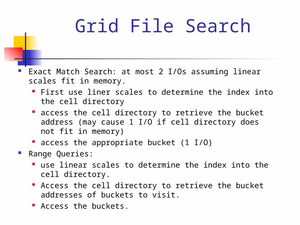
Exact Match Search: at most 2 I/Os assuming linear scales fit in memory.

First use liner scales to determine the index into the cell directory

access the cell directory to retrieve the bucket address (may cause 1 I/O if cell directory does not fit in memory)

access the appropriate bucket (1 I/O) Range Queries:

use linear scales to determine the index into the cell directory.

Access the cell directory to retrieve the bucket addresses of buckets to visit.

Access the buckets.

Grid File Insertions

Determine the bucket into which insertion must occur.

If space in bucket, insert. Else, split bucket

how to choose a good dimension to split? If bucket split causes a cell directory to split do so and adjust linear scales.

insertion of these new entries potentially requires a complete reorganization of the cell directory--- expensive!!!

Grid File Deletions Deletions may decrease the space utilization. Merge buckets

We need to decide which cells to merge and a merging threshold

Buddy system and neighbor system A bucket can merge with only one buddy in each dimension

Merge adjacent regions if the result is a rectangle

Tree-based PAMs Most of tb-PAMs are based on kd-tree kd-tree is a main memory binary tree for indexing k-dimensional points Needs to be adapted for the disk model

Levels rotate among the dimensions, partitioning the space based on a value for that dimension

kd-tree is not necessarily balanced

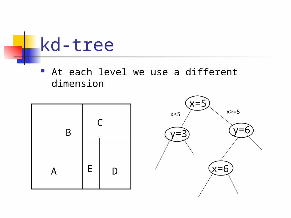
kd-tree At each level we use a different dimension

x=5

y=3 y=6

x=6A

BC

DE

x<5 x>=5

Kd-tree properties Height of the tree O(log2 n) Search time for exact match: O(log2 n)

Search time for range query: O(n1/2 + k)

kd-tree example

X=5

y=5 y=6

x=3

y=2

x=8 x=7

X=5 X=8

X=7X=3

Y=6

Y=2

External memory kd-trees (kdB-tree)

Pack many interior nodes (forming a subtree) into a block using BFS-travesal.

it may not be feasible to group nodes at lower level into a block productively.

Many interesting papers on how to optimally pack nodes into blocks recently published.

Similar to B-tree, tree nodes split many ways instead of two ways

insertion becomes quite complex and expensive. No storage utilization guarantee since when a higher level node splits, the split has to be propagated all the way to leaf level resulting in many empty blocks.

LSD-tree Local Split Decision – tree Use kd-tree to partition the space. Each partition contains up to B points. The kd-tree is stored in main-memory.

If the kd-tree (directory) is large, we store a sub-tree on disk

Goal: the structure must remain balanced: external balancing property

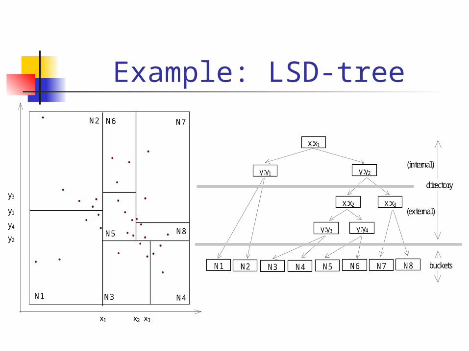
Example: LSD-tree

x1 x2 x3

y1

y3

y2

N1

N2 N6 N7

N8N5

N4N3

y4

N2 N3 N4 N5 N6 N7N1 N8

x:x1

y:y1 y:y2

x:x2 x:x3

y:y4y:y3

buckets

directory

(internal)

(external)

LSD-tree: main points Split strategies:

Data dependent Distribution dependent

Paging algorithm Two types of splits: bucket splits and internal node splits

PAMs Point Access Methods

Multidimensional Hashing: Grid File Exponential growth of the directory

Hierarchical methods: kd-tree based Storing in external memory is tricky

Space Filling Curves: Z-ordering Map points from 2-dimensions to 1-dimension. Use a B+-tree to index the 1-dimensional points

Z-ordering Basic assumption: Finite precision in the representation of each co-ordinate, K bits (2K values)

The address space is a square (image) and represented as a 2K x 2K array

Each element is called a pixel

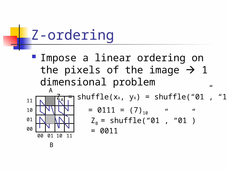
Z-ordering Impose a linear ordering on the pixels of the image 1 dimensional problem

00 01 10 1100

01

10

11

A

B

ZA = shuffle(xA, yA) = shuffle(“01”, “11”)

= 0111 = (7)10

ZB = shuffle(“01”, “01”) = 0011

Z-ordering Given a point (x, y) and the precision K find the pixel for the point and then compute the z-value

Given a set of points, use a B+-tree to index the z-values

A range (rectangular) query in 2-d is mapped to a set of ranges in 1-d

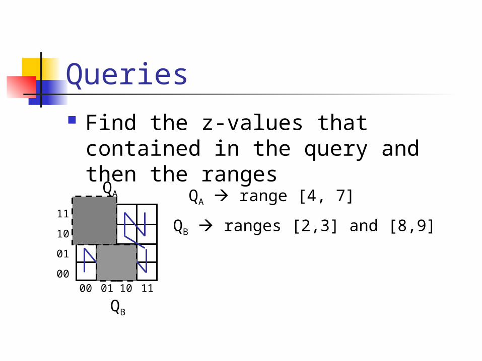
Queries Find the z-values that contained in the query and then the ranges

00 01 10 1100

01

10

11

QA range [4, 7]QA

QB

QB ranges [2,3] and [8,9]

Hilbert Curve We want points that are close in 2d to be close in the 1d

Note that in 2d there are 4 neighbors for each point where in 1d only 2.

Z-curve has some “jumps” that we would like to avoid

Hilbert curve avoids the jumps : recursive definition

Hilbert Curve- example It has been shown that in general Hilbert is better than the other space filling curves for retrieval [Jag90]

Hi (order-i) Hilbert curve for 2ix2i array

H1H2 ... H(n+1)

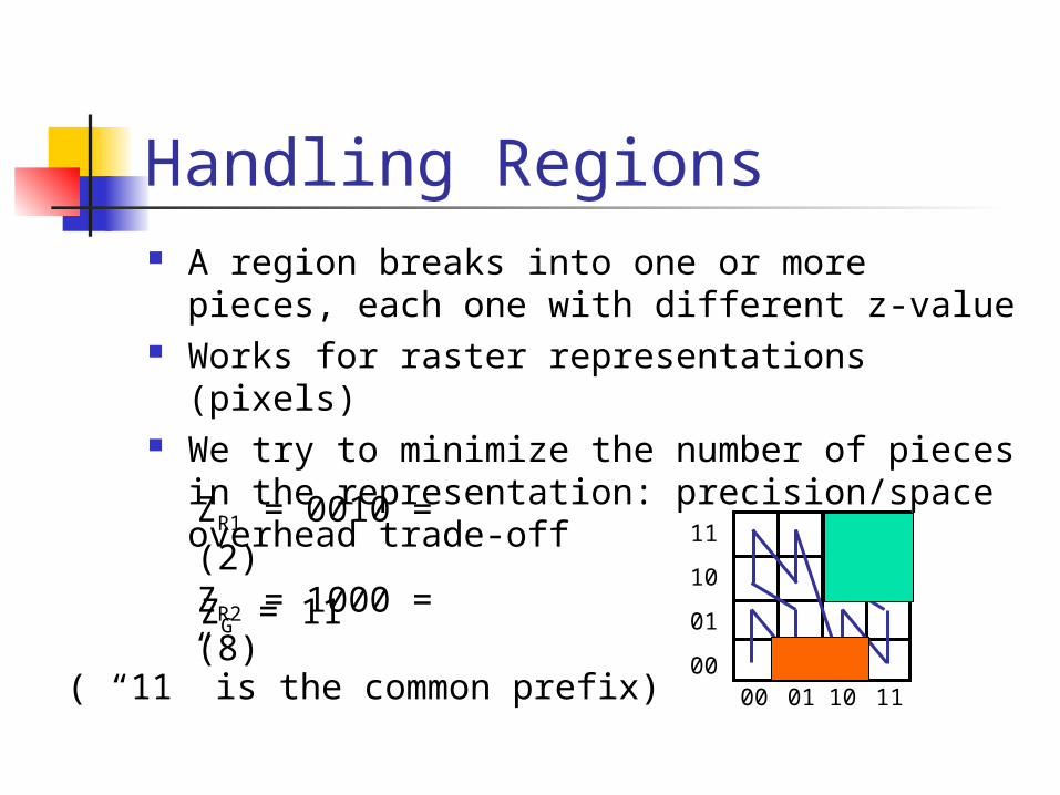
Handling Regions A region breaks into one or more pieces, each one with different z-value

Works for raster representations (pixels)

We try to minimize the number of pieces in the representation: precision/space overhead trade-off

00 01 10 1100

01

10

11ZR1 = 0010 = (2)ZR2 = 1000 = (8)

ZG = 11

( “11” is the common prefix)

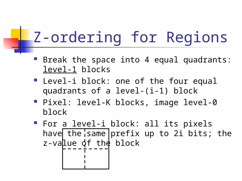
Z-ordering for Regions Break the space into 4 equal quadrants: level-1 blocks

Level-i block: one of the four equal quadrants of a level-(i-1) block

Pixel: level-K blocks, image level-0 block

For a level-i block: all its pixels have the same prefix up to 2i bits; the z-value of the block

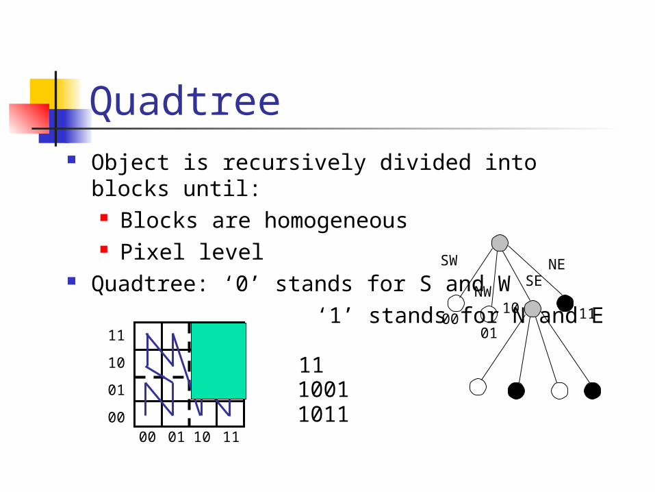
Quadtree Object is recursively divided into blocks until: Blocks are homogeneous Pixel level

Quadtree: ‘0 ’ stands for S and W ‘1 ’ stands for N and E

00 01 10 1100

01

10

11

SW

SENW

NE

110010

01

1110011011

Region Quadtrees Implementations

FL (Fixed Length) FD (Fixed length-Depth) VL (Variable length)

Use a B+-tree to index the z-values and answer range queries

Linear Quadtree (LQ)

Assume we use n-bits in each dimension (x,y) (so we have 2nx2n pixels)

For each object O, compute the z-values of this object: z1, z2, z3, …, zk (each value can have between 0 and 2n bits)

For each value zi we append at the end the level l of this value ( level l =log(|zi|))

We create a value with 2n+l bits for each z-value and we insert it into a B+-tree (l= log2(h))

B

A

C

A: 00, 01 = 00000001B: 0110, 10 = 01100010C: 111000,11 = 11100011

A:1, B:98, C: 227

Insert into B+-tree using Mb

Z-value, l | Morton block

Query Alg

WindowQ(query w, quadtree block b){ Mb = Morton block of b; If b is totally enclosed in w { Compute Mbmax Use B+-tree to find all objects with M values between Mb<=M<= Mbmax add to result } else { Find all objects with Mb in the B+-tree update result Decompose b into four quadrants sw, nw, se, ne For child in {sw, nw, se, ne}

if child overlaps with w WindowQ(w, child)

}}

z-ordering - analysis

Q: How many pieces (‘quad-tree blocks’) per region?

A: proportional to perimeter (surface etc)

z-ordering - analysis

(How long is the coastline, say, of Britain?

Paradox: The answer changes with the yard-stick -> fractals ...)

http://en.wikipedia.org/wiki/How_Long_Is_the_Coast_of_Britain%3F_Statistical_Self-Similarity_and_Fractional_Dimension

z-ordering - analysis

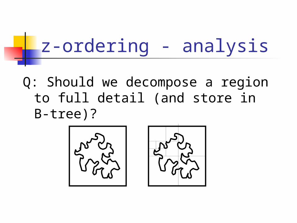
Q: Should we decompose a region to full detail (and store in B-tree)?

z-ordering - analysisQ: Should we decompose a region to full detail (and store in B-tree)?

A: NO! approximation with 1-5 pieces/z-values is best [Orenstein90]

z-ordering - analysis

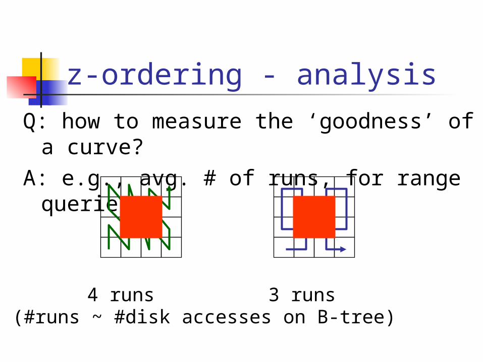
Q: how to measure the ‘goodness’ of a curve?

z-ordering - analysis

Q: how to measure the ‘goodness’ of a curve?

A: e.g., avg. # of runs, for range queries

4 runs 3 runs(#runs ~ #disk accesses on B-tree)

z-ordering - analysisQ: So, is Hilbert really better?A: 27% fewer runs, for 2-d (similar for 3-d)

Q: are there formulas for #runs, #of quadtree blocks etc?

A: Yes, see a paper by [Jagadish ’90]