Spatial Stochastic Vehicle Traffic Modeling for VANETs

Jingqiu Guo1, Yibing Wang2

1. College of Transportation Engineering, Tongji University, China

2. College of Civil Engineering, Zhejiang University , China

I. INTRODUCTION Vehicular Ad hoc NETworks (VANETs) [1-8] aim to make driving a safer, more

enjoyable, and more efficient experience. In VANETs, wireless-equipped vehicles form a network spontaneously while traveling along the road. Through vehicle-to-vehicle (V2V) and vehicle-to-infrastructure (V2I) communications, vehicles can communicate with each other via a single-or multi-hop ad hoc connection, or with the aid of stationary roadside units.

All VANETs applications highly depend on reliable dissemination of time-critical information to/among connected vehicles on road. Network connectivity [5, 11, 16-18] is a fundamental requirement for VANETs, i.e. all vehicles on a road section should be able to communicate with each other either directly or by multiple hops via intermediate vehicles. The connectivity of VANETs is directly related to the density of vehicles on the road, their speed distribution, and transmission power. Vehicles can be thought almost surely connected if traffic density is very high. In the free flow condition, however, connectivity degrades due to large inter-vehicle spacing and limited radio ranges of DSRC. Moreover, individual vehicles are of strong mobility, and the network topology of VANETs can be highly dynamic. Thus, VANETs may experience frequent network fragmentation in the case of traffic sparsity and/or low market penetration of equipped vehicles. This has profound impacts on network connectivity, especially in the early stage of the VANETs deployment [6, 9, 19, 20].

The VANETs connectivity has attracted considerable interests recently [1, 3-5, 8-11, 16-22]. The probabilistic distributions of inter-vehicle spacing [7] play a crucial role in the study of connectivity. Three approaches have been tried to handle this issue. First, a lot of works simply assume that the concerned distribution is exponential, equivalently, the number of vehicles within a road section is Poisson distributed, see e.g. [2, 8, 18, 21-23]. Second, some researchers attempted to handle the issue analytically, and basically two models were employed: the M/G/∞ queueing model, see e.g. [6, 9, 17, 19], and Yousefi’s model [1, 5, 11]. Both models indicate that the spatial vehicle traffic distribution is exponential/Poisson. Third, field data was utilized to evaluate the hypothesis of Poisson/exponential distribution for spatial vehicular traffic [16]. This paper follows the second/analytical approach to further study the issue.

In traffic engineering, it is rather easy to measure the number of vehicles passing a given point of a highway (N) as well as the time intervals of vehicle passage (T). It is well known [24, 25] that N is typically Poisson distributed if the prevailing traffic is in the free flow to moderate condition; equivalently, T is exponentially distributed. On the other hand, it is rather troublesome (e.g. based on aeroplane photographing) to obtain real data on the spatial number of vehicles within a road section (M) and the corresponding inter-vehicle spacing (S). Consequently, much less information of M and S can actually be found in the literature of traffic engineering.

Since many researchers take the Poisson and exponential assumption of M and S as the start point of their connectivity studies, it is very important to ensure that the assumption is correct. So far, convincing real data evaluation was only found in [16]. Also, there has not been sufficient analytical studies, except for the M/G/∞ model and Yousefi’s model. The M/G/∞ model highly relies on the M/G/∞ queueing theory, and is not transparent. Yousefi model requires that vehicle speeds be classified into a finite number of discrete levels. In this paper we intend to develop a model that is more general and transparent than the two previous ones, involving only ordinary assumptions and allowing for a general speed distribution of vehicles. This work also aims to determine an explicit mathematical expression for the distributions of inter-vehicle spacing, which was not available before. Last but not least, even in transportation science and traffic engineering, there is currently a knowledge gap concerning the spatial distribution of vehicular traffic, to which the authors also wish to contribute via this work.

II. PROBLEM STATEMENT

Based on literature review, the current studies on connectivity focus on the case of traffic

sparsity, because connectivity would otherwise not be of a major concern. Therefore, it is reasonable to assume that vehicle arrivals at the certain point of road form a Poisson process. With this in mind, we are intended to consider a problem as illustrated with Fig. 3. The displayed multi-lane highway is initially empty. Vehicles start to arrive at the entrance in a Poisson process. Assume that each arriving vehicle obtains a speed randomly from a general speed distribution, independently of other vehicles, and keeps moving along the highway at this speed. Considering traffic sparsity, we also assume there is no time loss during the process of vehicle overtaking. The question is that, after a sufficiently long time period, how vehicles are distributed within any road section [a, b]. The answer is given with Theorem 1 below.

III. MAIN RESULTS

Consider the scenario depicted with Fig. 3. The highway is semi-infinite. Vehicles enter

the highway at intants 0 = 𝜏! < 𝜏! < 𝜏! < ⋯ in a Poisson process of rate 𝜆. The vehicle entering at time 𝜏! picks a velocity 𝑣! and travels at this speed. Assume that all 𝑣!’s are sampled from a common distribution, with the probability density function 𝑓!(𝑣) and cumulative distribution function 𝐹!(𝑣). Theorem 1. The spatial distribution of vehicles as depicted in Fig. 3 constitutes a homogeneous Poisson process of rate 𝛌 𝟏

𝒗𝒇𝑽(𝒗)𝒅𝒗

!𝟎 < ∞.

Remark 1. The number of vehicles with a road section [a, b] is Poisson distributed with 𝜆(𝑏 − 𝑎) !

!𝑓!(𝑣)𝑑𝑣

!! < ∞.

Remark 2. According to the postulates of Theorem 1, vehicles enter the highway at rate 𝜆. 𝜆 actually represents the mean flow at the highway entry. Since each vehicle runs at a constant speed, the mean flow is constant along the highway. Note that 𝜆 !

!𝑓!(𝑣)𝑑𝑣!! =

𝜆𝐸 !! = !

! !!

!!, and moreover 𝐸 !! = lim!→!

!!

!!!

!!!! , and hence 𝐸 !

!

!! stands for the

space mean speeds of vehicular traffic [24, 25]. Thus, what the Poisson rate 𝜆 !!𝑓! 𝑣 𝑑𝑣!

! represents is actually mean traffic density. As such, Theorem 1 tells that the spatial distribution of vehicles along the highway is Poisson with the rate equal to mean traffic density. Remark 3. In traffic engineering, knowledge about the temporary distribution of passing vehicles at a given location is well accessible [24, 25] while that of the spatial distribution of vehicles within a road section is quite unknown. Theorem 1 actually sets a bridge between vehicular temporary distribution of rate 𝜆 (number of vehicles per unit time) and vehicular spatial distribution of rate 𝜆 !

!𝑓! 𝑣 𝑑𝑣!! (number of vehicles per unit distance); see also the

arrow in Fig. 3. Remark 4. It is commonly recognized that the penetration rate of DSRC-equipped vehicles is quite low in an early stage of the VANETs deployment. Equipped vehicles could then be thought uniformly distributed among road vehicles. Denoting by 𝑝 the penetration rate and following the principle of “Thinning of a Poisson process”, we can easily determine that the number of equipped vehicles within any road section of unit length is Poisson distributed with rate 𝜆𝑝 !

!𝑓!(𝑣)𝑑𝑣

!! . Interestingly, field data evaluations in [16] indicate that, if the

prevailing traffic condition is not free-flow, but the penetration rate is sufficiently low, the spatial number of equipped vehicles could still be Poisson.

IV. SIMULATION STUDIES This section intends to demonstrate the conclusion of Theorem 1 via simulation. The

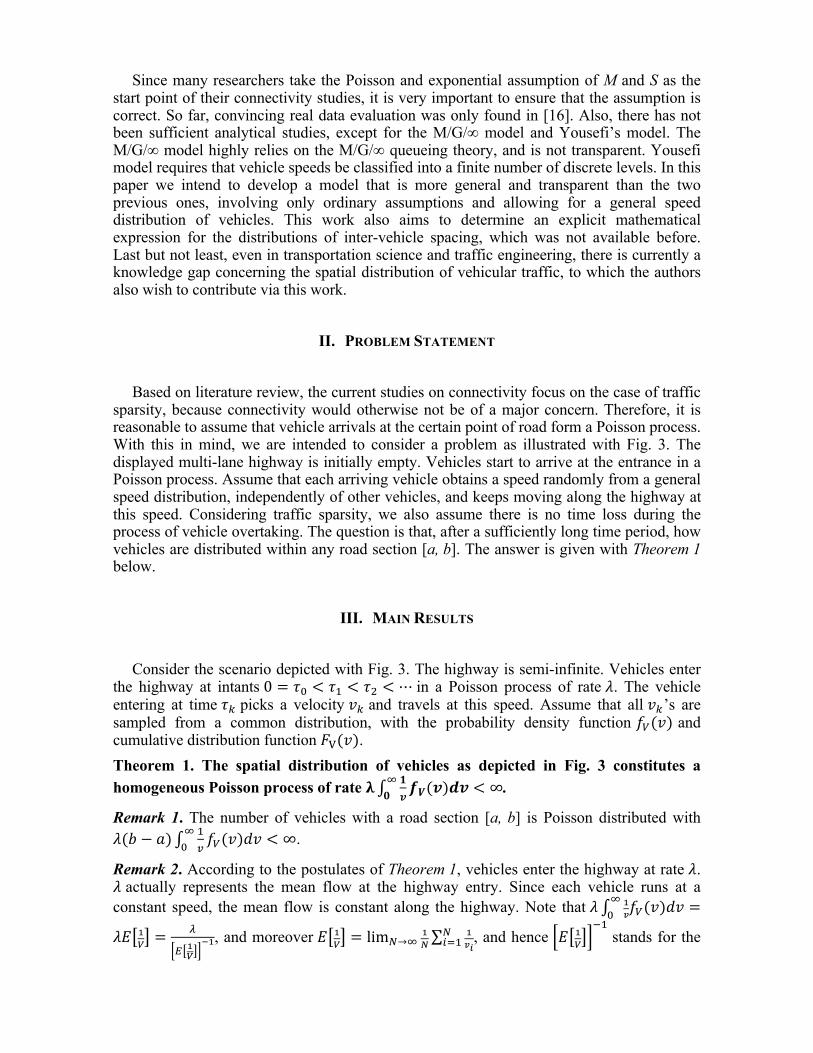
simulation environment is displayed in Fig. 4, whereby Poissonian vehicle flow of rate 𝜆 enters over the period [0, ∞) a highway stretch that is initially empty. The initial speeds of all vehicles are sampled at the entrance from a common distribution of PDF 𝑓!(𝑣), and each vehicle keeps running at her initial speed. Since the focus of this research is on the free flow condition, no time loss is assumed during the process of vehicle overtaking.

A number of potential impact factors taken into account are: (a) the sampling time instant 𝒕 > 0; (b) the distance between the entrance and the start of the examined road section, i.e. 𝒙𝟏 in

Fig. 4; (c) the length of the examined road section, i.e. 𝒙𝟐 − 𝒙𝟏; (d) the rate 𝝀 of Poisson inflow; (e) the PDF 𝒇𝑽(𝒗).

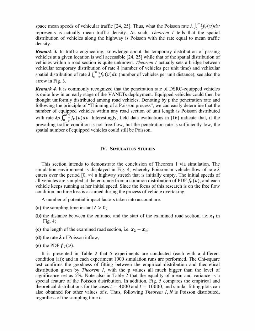
It is presented in Table 2 that 5 experiments are conducted (each with a different condition (a)); and in each experiment 1000 simulation runs are performed. The Chi-square test confirms the goodness of fitting between the empirical distribution and theoretical distribution given by Theorem 1, with the p values all much bigger than the level of significance set as 5%. Note also in Table 2 that the equality of mean and variance is a special feature of the Poisson distribution. In addition, Fig. 5 compares the empirical and theoretical distributions for the cases 𝑡 = 4000 and 𝑡 = 10000, and similar fitting plots can also obtained for other values of 𝑡. Thus, following Theorem 1, 𝑁 is Poisson distributed, regardless of the sampling time 𝑡.

V. CONCLUSION In this paper we have proved that under the free flow condition the distribution of the

spatial number of vehicles along a highway is Poisson, and hence inter-vehicle spacing are exponentially distributed. The proof is generic without specific requirements for the involved speed distributions. This theoretical result that has also been demonstrated with simulation studies is very important for the connectivity study of VANETs. Table 1. Fixed conditions (b)-(e).

Table 2. Varying condition (a).

t (s)

Simulated results

Theoretical results

(Theorem 1)

Chi-square test

(Significance level of 5%)

E[N] Var[N] E[N] = Var[N] P value

2000 37.7 37.7

38

0.407 4000 37.6 39.4 0.692 6000 37.7 38.7 0.884 8000 37.9 38.5 0.221 10000 38.2 37.5 0.987

𝑎   𝑏  

… …

temporal distribution of vehicle arrivals

spatial distribution of running vehicles

0  

… … …

the start of a highway a highway section

Fig. 3. An illustrative diagram for our model.

𝑥! 7 km 𝑥! − 𝑥! 3 km λ 720 veh/h 𝑓!(𝑣) Normal (17, 4)

0 𝑥1 𝑥2

𝑓𝑉(𝑣) 𝜆 𝑁(𝑡) ,

Fig. 4. Simulation environment.

(a) (b)

Fig. 5. The comparison of empirical and theoretical distributions: (a) 𝑡 = 4000 s; (b)

 𝑡 = 10000 s.