172

SPATIAL STOCHASTIC FRONTIER MODELS: ACCOUNTING FOR UNOBSERVED LOCAL DETERMINANTS OF INEFFICIENCY

Alexandra M. SchmidtAjax R. B. MoreiraThais C. O. FonsecaSteven M. Helfand

Originally published by Ipea in October 2006 as number 1220 of the series Texto para Discussão.

DISCUSSION PAPER

172B r a s í l i a , J a n u a r y 2 0 1 5

Originally published by Ipea in October 2006 as number 1220 of the series Texto para Discussão.

SPATIAL STOCHASTIC FRONTIER MODELS: ACCOUNTING FOR UNOBSERVED LOCAL DETERMINANTSOF INEFFICIENCY

Alexandra M. Schmidt1

Ajax R. B. Moreira2

Thais C. O. Fonseca3

Steven M. Helfand4

1. Associate professor in Statistics at the Federal University of Rio de Janeiro (UFRJ).2. Researcher fellow of the Aplied Economic Research Institute (Ipea).3. PhD student of the Statistics Department at the University of Warwick, UK.4. Associate professor of Economics at the University of California, USA.

DISCUSSION PAPER

A publication to disseminate the findings of research

directly or indirectly conducted by the Institute for

Applied Economic Research (Ipea). Due to their

relevance, they provide information to specialists and

encourage contributions.

© Institute for Applied Economic Research – ipea 2015

Discussion paper / Institute for Applied Economic

Research.- Brasília : Rio de Janeiro : Ipea, 1990-

ISSN 1415-4765

1. Brazil. 2. Economic Aspects. 3. Social Aspects.

I. Institute for Applied Economic Research.

CDD 330.908

The authors are exclusively and entirely responsible for the

opinions expressed in this volume. These do not necessarily

reflect the views of the Institute for Applied Economic

Research or of the Secretariat of Strategic Affairs of the

Presidency of the Republic.

Reproduction of this text and the data it contains is

allowed as long as the source is cited. Reproductions for

commercial purposes are prohibited.

Federal Government of Brazil

Secretariat of Strategic Affairs of the Presidency of the Republic Minister Roberto Mangabeira Unger

A public foundation affiliated to the Secretariat of Strategic Affairs of the Presidency of the Republic, Ipea provides technical and institutional support to government actions – enabling the formulation of numerous public policies and programs for Brazilian development – and makes research and studies conducted by its staff available to society.

PresidentSergei Suarez Dillon Soares

Director of Institutional DevelopmentLuiz Cezar Loureiro de Azeredo

Director of Studies and Policies of the State,Institutions and DemocracyDaniel Ricardo de Castro Cerqueira

Director of Macroeconomic Studies and PoliciesCláudio Hamilton Matos dos Santos

Director of Regional, Urban and EnvironmentalStudies and PoliciesRogério Boueri Miranda

Director of Sectoral Studies and Policies,Innovation, Regulation and InfrastructureFernanda De Negri

Director of Social Studies and Policies, DeputyCarlos Henrique Leite Corseuil

Director of International Studies, Political and Economic RelationsRenato Coelho Baumann das Neves

Chief of StaffRuy Silva Pessoa

Chief Press and Communications OfficerJoão Cláudio Garcia Rodrigues Lima

URL: http://www.ipea.gov.brOmbudsman: http://www.ipea.gov.br/ouvidoria

DISCUSSION PAPER

A publication to disseminate the findings of research

directly or indirectly conducted by the Institute for

Applied Economic Research (Ipea). Due to their

relevance, they provide information to specialists and

encourage contributions.

© Institute for Applied Economic Research – ipea 2015

Discussion paper / Institute for Applied Economic

Research.- Brasília : Rio de Janeiro : Ipea, 1990-

ISSN 1415-4765

1. Brazil. 2. Economic Aspects. 3. Social Aspects.

I. Institute for Applied Economic Research.

CDD 330.908

The authors are exclusively and entirely responsible for the

opinions expressed in this volume. These do not necessarily

reflect the views of the Institute for Applied Economic

Research or of the Secretariat of Strategic Affairs of the

Presidency of the Republic.

Reproduction of this text and the data it contains is

allowed as long as the source is cited. Reproductions for

commercial purposes are prohibited.

JEL: C01; C11.

SINOPSENeste texto, analisamos a produtividade de estabelecimentos agrícolas localizados em370 municípios da região Centro-Oeste do Brasil. Propomos um modelo de fronteiraestocástica de produção com estrutura espacial latente que representa osdeterminantes não-observados da ineficiência da produtividade da agropecuária. Essecomponente espacial condiciona a distribuição da ineficiência. Usamos o paradigmabayesiano para estimar os modelos propostos. Foram exploradas duas distribuiçõesdiferentes para este termo, a normal truncada e a exponencial, e utilizamos duasespecificações para a variável latente, suposta independente entre os municípios, oudependente dos municípios vizinhos segundo um modelo auto-regressivo espacial.

O procedimento de inferência considera explicitamente todas as incertezasquando incluímos o termo espacial. Como a distribuição a posteriori não tem umaexpressão analítica, utilizamos técnicas estocásticas da simulação para obter amostrasdessa distribuição. Foram adotados dois critérios que avaliam o desempenho domodelo, e os dois indicaram que o componente espacial latente incorpora informaçãoadicional a um modelo que já contém informação local observada.

ABSTRACTIn this paper, we analyze the productivity of farms across n = 370 municipalitieslocated in the Center-West region of Brazil. We propose a stochastic frontier modelwith a latent spatial structure to account for possible unknown geographical variationof the outputs. This spatial component is included in the one-sided disturbance term.We explore two different distributions for this term, the exponential and thetruncated normal. We use the Bayesian paradigm to fit the proposed models. We alsocompare between an independent normal prior and a conditional autoregressive priorfor these spatial effects. The inference procedure takes explicit account of theuncertainty when considering these spatial effects. As the resultant posteriordistribution does not have a closed form, we make use of stochastic simulationtechniques to obtain samples from it. Two different model comparison criteriaprovide support for the importance of including these latent spatial effects, even afterconsidering covariates at the municipal level.

SUMMARY

1 INTRODUCTION 7

2 MOTIVATION 8

3 PROPOSED MODEL 9

4 INFERENCE PROCEDURE 11

5 EMPIRICAL ANALYSIS 13

6 CONCLUDING REMARKS AND FUTURE WORK 17

ACKNOWLEDGEMENTS 18

REFERENCES 18

1 Introduction

Stochastic frontier models have been widely used to describe productivity and firmefficiency. These models were introduced by Aigner et al. (1977) and, Meeusenand van den Broeck (1977). A stochastic frontier production function decomposesoutput into three components. The first is a deterministic component that includesinputs in the production function and other variables that affect productivity andare correlated with the inputs. The second is an asymmetric stochastic componentthat captures the inefficiency of each producer (measured as the distance to thefrontier). The moments of the distribution of the inefficiency component mightdepend on a set of variables–not all of which are observed. The third component ofthe model is a random disturbance. There are different proposals in the literaturefor the distribution of the inefficiency component: the exponential (Meeusen andvan den Broeck, 1977), the half-normal (Aigner et al., 1977), the truncated normal(Stevenson, 1980), the gamma (Greene, 1990) and, the log-normal (Migon, 2006).

In many real world examples of production, local conditions affect productivity.In the context of agriculture, for example, differences across localities in transporta-tion infrastructure, soils and climate, human capital of the local labor force, andother factors, can create systematic variation in the efficiency of agricultural pro-duction across localities. Local determinants of efficiency can be estimated withfixed or random effects. Alternatively, when information is available to describe thelocal determinants, these variables can be included directly in the stochastic fron-tier model. In the first case, local effects are measured fully but it is not possibleto interpret the determinants of the effects, while in the second case interpretationis feasible but the vector of determinants included in the model does not exhaustthe list of possible determinants. An additional local effect remains, and failureto account for this will lead to bias in the estimated coefficients on the includedvariables.

The novelty of our approach lies in the introduction of a municipal level latenteffect in the modelling of the inefficiencies. More specifically, we believe that theinefficiency of unit j, j = 1, · · · , ni in municipality i, i = 1, · · · , n depends on whichmunicipality it is located in. Our model combines models from the stochastic frontierand spatial econometric literatures. Inference is conducted following the Bayesianparadigm. See Koop and Steel (2001) and Kumbhakar and Tsionas (2005) for a re-view of the use of the Bayesian paradigm for this class of models and, Anselin (1988)and Gamerman and Moreira (2004) for a review on spatial econometric models.

A priori, we assume that the inefficiencies, uij, for i = 1, · · · , n and j = 1, · · · , niare conditionally exchangeable within each municipality i. More formally, the inef-ficiency uij of agent j = 1, · · · , ni, located in municipality i = 1, · · · , n, is estimatedconditioned on the unobserved local characteristics αi, uij ∼ g(i), where g is a pos-itive and asymmetric probability density function, depending on αi. This compo-nent αi, which represents the unobserved local characteristics in each municipality,is a common component among the inefficiencies of all agents in each municipality.Therefore, the inefficiencies of units which are in the same municipality are gener-ated from the same distribution. However, these distributions are allowed to differ

across the region. This is because we assume that agents are heterogeneous, andthat part of this heterogeneity might derive from the location of the agents. Onemight assume, a priori, that these latent effects are either independent or spatiallystructured. The latter means that αi − αk, ∀i 6= k = 1, · · · , n would tend to besmaller for municipalities that are closer together. Therefore, we also discuss theprior distribution of these latent effects.

Frequently, in the stochastic frontier literature, the observations are availablein the form of panel data. Here, however, the replicates are obtained across spaceand not time, and we have many observations within each of the n municipalities.Our aim is to model this spatial heterogeneity even after accounting for a possibleset of covariates at the municipality level which might affect the productivity ofeach unit. Tsionas (2002) proposes stochastic frontier models with random coeffi-cients to separate technical inefficiency from technological differences across firms.On the other hand, Greene (2005) extends fixed effects models in the context ofthe stochastic frontier literature with a variety of approaches to incorporate firmspecific heterogeneity. From a spatial perspective, Druska and Horrace (2004) con-sider generalized moments estimation of panel data assuming a decomposition ofthe error term as the sum of two components: one that is spatially structured andthe other that is white noise. This spatial component is modelled through a simul-taneous autoregressive model. See Anselin (1988) for details. Helfand and Levine(2004) and Sampaio de Souza et al. (2005) employ a similar approach. First, theyestimate Data Envelopment Analysis (DEA) technical efficiency scores for munici-palities spread over a region. After computing the efficiency scores, they use either aspatial SUR or a simultaneous autoregressive model, respectively, to investigate thedeterminants of those scores. In other words, both papers mentioned above performthe inference procedure in two steps, taking no explicit account of the uncertaintyin the estimation of the efficiencies.

This paper is organized as follows. Section 2 provides the economic motivationfor the problem and describes the data set to be analyzed. Section 3 discusses theproposed model, and in Section 4 the inference procedure is described. Section 5presents the analysis of the data under the proposed model. As we explore differentmodel specifications for the data, two model comparison criteria, one based on thatsuggested by Gelfand and Ghosh (1998) and the other on that by Spiegelhalter et al.(2002), are described and performed. Finally, Section 6 concludes the paper anddescribes future avenues for research.

2 Motivation

This article is part of a larger research project which uses microdata from the1995/96 Agricultural Census in Brazil to study the determinants of agriculturalproductivity. The project is motivated by the observation that Brazil has one ofthe most unequal distributions of land holdings in the world, and an extremely highrate of rural poverty. In the past decade, a series of governments have pursued anaggressive policy of land reform. Brazil is also among the largest producers and ex-

porters in the world of many agricultural products. A deeper understanding of thedeterminants of productivity in Brazilian agriculture has important implications forreducing rural poverty by increasing productivity and income among small farm-ers, and for relaxing constraints on macroeconomic growth by increasing foreignexchange earnings.

Here we concentrate on a sample of farms in the Center-West region of Brazil.This region contained three states, 426 municipalities, and over 240,000 farms in1996. From this region, we chose a random sample of 25,494 farms spread overn=370 municipalities. In order to reduce certain types of heterogeneity that are notthe principal focus of this paper, we restricted the sample to (a) owner operatedfarms, (b) farms that hired one or more permanent workers, and (c) farms thatused inputs relatively intensively (identified as farms in the upper half of the dis-tribution of input expenditures per hectare)1. Because the choice of which outputsto produce is endogenous, and we are interested in comparing the efficiency withwhich agricultural producers transform inputs into numerous outputs through theCenter-West, we follow standard practice of using an output quantity index as ourdependent variable (see e.g. Coelli et al. (1998); Koop and Steel (2001)).

3 Proposed Model

Assume observations are available in the form of panel data. However, here, replica-tions are at the municipal level. Let yij be the logarithm of output for municipalityi, i = 1, 2, · · · , n and unit j, j = 1, 2, · · · , ni. We consider that observations arebeing generated through the following structure

yij = f(xij,β) + γ ′zi + δ′cih − uij(αi) + εij εij ∼ N(0, σ2), (1)

whereN(0, σ2) denotes the zero mean normal distribution with variance σ2, f(xij,β)represents the production function, with xij being a vector of dimension q1 of farmspecific inputs, and β a vector of their respective coefficients. The vector zi com-prises all the covariates, say q2, which vary at the municipal level, and might influ-ence the outputs. cih, of dimension q3, corresponds to dummy variables indicatingfarms size classes.

The component uij(.) models the inefficiency of unit j at location i and is in-dependent of εij. It is described as a function of a latent effect, αi, which variesacross the municipalities. We consider two different distributions for the inefficiencycomponent, uij(.) in equation (1). More specifically, we either model uij as

(uij | αi, τ 2) ∼ N+(αi, τ2) (2)

or as

uij | θi ∼ exp(1/θi) with log θi = αi, (3)

1In our larger research project on agricultural productivity, we examine all farm types andstudy the determinants of differences in productivity across these types of farms.

where N+(a, b) denotes the normal distribution truncated at zero, whose associatednormal has mean a and variance b, and exp(1/θ) denotes the exponential distributionwith mean θ. It is worth noting that the distribution in equation (2) states that theuij are exchangeable at the municipal level, conditioned on αi and τ 2. On the otherhand, in equation (3), they are exchangeable, at the municipal level, conditionedonly on θi. Notice that these latent effects are introduced in the second level ofhierarchy, therefore they do not affect the Yij’s directly. If the random effects wereintroduced in the mean of Yij we might get some correlation between zi and αi.This kind of centering provides more stable computation. See, for example, Gelfandet al. (1996) and Papaspiliopoulos et al. (2003). If there are no municipality levelcovariates, one might consider introducing αi directly in the mean structure of Yij.We discuss this further in Section 5.

As the inference procedure is made through the Bayesian Paradigm, an impor-tant issue is the effect of the prior distribution associated to the random effects αi’s.The simplest choice is to assume a priori that the αi’s are all independent amongthemselves, that is αi ∼ N(0, ψ2), ∀i = 1, 2, · · · , n. However, as the observationsare being made across municipalities, we would expect these random effects to bespatially correlated. Due to the geographical characteristics of the data, it is naturalto expect that the inefficiencies of units which are located in neighboring munici-palities are of similar magnitude. That is, the magnitude of the inefficiencies mightvary smoothly across the region. For this reason, following Besag et al. (1991), weassume a conditional autoregressive (CAR) prior for α = (α1, · · · , αn)′, that is

(αi |αk, k 6= i) ∼ N(mi, vi) where

mi =

∑k∈ ςiWikαk∑k∈ ςiWik

and vi =ψ2∑

k∈ ςiWik

(i, k = 1, · · · , n), (4)

where ςi is the set containing the neighboring municipalities of i. We denote thisprior as α ∼ CAR(ψ2). It is common practice to consider a 0 − 1 neighborhoodstructure, such that Wik = 1 if i and k share boundaries and 0 otherwise. In thiscase, we have that

mi =

∑k∈ ςi αk

n∗iand vi =

ψ2

n∗i,

where n∗i is the number of neighbors of municipality i. Notice that here, ψ2 is thevariance of the conditional distribution of (αi | αk, k 6= i), therefore its interpretationis not straightforward, that is, it is not the same as when we assume that theserandom effects are independent a priori. It is worth mentioning that the conditionaldistribution in equation (4) leads to an improper joint distribution for α. This isnot a problem, as we make clear in Section 4.

Assigning a CAR prior to the random effects αi means that they are correlated apriori, therefore, if we model uij as in equation (2) we are implicitly assuming thatthe Yij are independent among themselves conditioned on the inefficiencies, uij’s.

Let y = (y11, · · · , y1n1 , · · · , yn1, · · · , ynnn)′ represent a random sample of thelogarithm of the outputs at location i = 1, 2, · · · , n and unit j = 1, 2, · · · , ni. Under

the specification in (2) or in (3), the likelihood is given by

p(y | xij,β, uij, τ 2, σ2) ∝(σ2)−n/2

exp

{− 1

2σ2

n∑i=1

ni∑j=1

(yij − f(xij,β)− γ ′zi − δ′cij + uij)2

}. (5)

Assuming uij is distributed as in (2), Stevenson (1980) and Broeck et al. (1994)show that when integrating the likelihood above with respect to uij one obtains

p(y | xij,β, αi, σ2) ∝n∏i=1

ni∏j=1

1√σ2 + τ 2

φ

(yij − f(xij,β)− γ ′zi − δ′cij + αi√

σ2 + τ 2

)

×Φ

(αi√σ2 + τ 2

στ− τ(yij − f(xij,β)− γ ′zi − δ′cij + αi)

σ√σ2 + τ 2

)Φ−1

(αiτ

), (6)

which is a skew normal distribution as described in Domınguez-Molina and Gonzalez-Farıas (2003). On the other hand, following the specification for uij as in (3) and,marginalizing the likelihood with respect to uij, Stevenson (1980) and Broeck et al.(1994) show that

p(y | xij,β, αi, σ2) ∝n∏i=1

ni∏j=1

θ−1ij exp

{−mij

θij− σ2

2θ2ij

}Φ(mij

σ

), (7)

where mij = f(xij,β) + γ ′zi + δ′cij − yij − σ2

θij, Φ(x) is the cumulative distribution

and φ(x) is the probability density function of the standard normal distributionevaluated at point x. These marginalizations with respect to uij will prove useful inthe simulation methods which will be described in the next Section.

4 Inference Procedure

Following the Bayesian paradigm the model specification is complete after assigninga prior distribution to all unknowns (parameters) in the model. In the previousSection we only discussed the prior distribution of the latent random effects αi, andof the one-sided disturbance term. Here we will discuss the prior distribution ofthe remaining parameters in the model. Then, following Bayes’ theorem, we willobtain the kernel of the posterior distribution of the parameter vector. Lastly, wewill describe how to make inference from the resultant posterior distribution.

Let θ comprise the parameter vector, such that θ = (β0,β,γ, δ,α, ψ2, τ 2, σ2)′.

Initially, we assume that all components of θ are independent a priori. Therefore,the joint density prior distribution for θ is given by

p(θ) =

q1∏i=0

p(βi)

q2∏j=1

p(γj)

q3∏k=1

p(δk) p(α | ψ2) p(ψ2) p(τ 2) p(σ2).

Following standard procedures, for the coefficients βi, γj, and δk i = 1, · · · , q1,j = 1, · · · , q2, k = 1, · · · , q3 we assign a zero mean normal prior distributions with

variance (σ2β) fixed at some big value. For the variances τ 2 and σ2 we assign inverse

gamma prior distributions with both parameters equal to ε, i.e. τ 2 ∼ IG(ε, ε), whereε is fixed at some small number, say 0.1, to describe our prior ignorance about theseparameters. Some care must be taken when assigning the prior distribution forψ2, the variance of the CAR distribution. This prior cannot be too uninformative,as this is a non-identifiable parameter in the sense of Dawid (1979). We assign aninverse gamma prior, IG(aψ, bψ), whose mean is equal to the OLS estimate based onan independent stochastic frontier model, with some fixed variance. Once the priordistribution has been assigned, following Bayes’ theorem, the posterior distributionof θ is proportional to the likelihood function times the prior, which considering,for example, the specification in (2), results in

p(θ | y) ∝ p(y | xij,θ) p(θ)

∝n∏i=1

ni∏j=1

1√σ2 + τ 2

φ

(yij − f(xij,β)− γ ′zi − δ′cij + αi√

σ2 + τ 2

)

×Φ

(αi√σ2 + τ 2

στ− τ(yij − f(xij,β)− γ ′zi − δ′cij + αi)

σ√σ2 + τ 2

)Φ−1

(αiτ

)×

q1∏i=0

exp

{− 1

2σ2β

β2i

}q2∏i=1

exp

{− 1

2σ2β

γ2i

}q3∏i=1

exp

{− 1

2σ2β

δ2i

}(8)

×(ψ2)−n/2

exp

{− 1

2ψ2

n∑i=1

∑j<i

Wij(αi − αj)2

}(ψ2)−(aψ+1)

exp

{− bψψ2

}×(τ 2)−(ε+1)

exp{− ε

τ 2

}(σ2)−(ε+1)

exp{− ε

σ2

}.

The equation above does not have an analytical closed form. Therefore, simulationmethods are needed to make inference about p(θ | y). We make use of Markovchain Monte Carlo (MCMC) methods, in particular the Gibbs sampling algorithm(Gelfand and Smith, 1990) with some steps of the Metropolis-Hastings (Hastings,1970) and the slice sampling (Neal, 2003) algorithms. Gamerman and Lopes (2006)give more details about these sampling schemes.

As described in Gamerman and Lopes (2006), the Gibbs sampler is a MCMCscheme where the transition kernel of the Markov chain is based on the full con-ditional posterior distributions, π(θi | θ−i), where θ−i = (θ1, · · · , θi−1, θi+1, · · · , θp),and p is the dimension of the parameter vector. Because of the marginalization in(6) or in (7), the full conditional distributions of the elements of β do not follow anyknown distribution. We make use of a Metropolis-Hastings random walk to samplefrom this full conditional. From our experience, the speed of convergence of thechains might be sensitive to the starting values of the elements of β, γ, and δ. Wesuggest to start the chain from their OLS estimates based on a multiple regressionwithout the inefficiency component. In the case of the variances, σ2 and τ 2, theirfull conditionals do not have an analytical closed form. Here we also suggest theuse of a Metropolis-Hastings random walk step for log σ2 and log τ 2, respectively.

On the other hand, ψ2 has an inverse gamma posterior full conditional distributionregardless of whether an independent normal or a CAR prior is assigned to α.

Our main challenge when implementing the algorithm is the sampling of each αi.Notice, that we have as many αi’s as the number of municipalities in the sample.As the use of a random walk Metropolis-Hastings step requires the tuning of thevariance of the proposal distribution, we prefer to use the slice sampling algorithm(Neal, 2003) to sample from π(αi | θ−αi ,y). The slice sampler is an auxiliary variableMCMC algorithm. It is based on the idea of slicing the target distribution (thefull conditional of αi in our case) horizontally at the contour level of a uniformlydistributed variable U(0, π(αi | .)). See Gamerman and Lopes (2006) for moredetails. Recall that the CAR prior as defined in (4) results in an improper jointdistribution for the spatial effects. Following Besag et al. (1995) as a remedy weimpose the constraint

∑i αi = 0 after each iteration of the Gibbs sampler.

It is worth mentioning the computational advantage of marginalizing the like-lihood with respect to uij. While running the MCMC, we avoid updating theseparameters and the algorithm becomes faster. After convergence has been reached,we can use the samples from the elements of θ to obtain posterior samples of theefficiencies, exp(−uij(.)), through the posterior of uij.

5 Empirical Analysis

In this Section we fit the proposed model to the sample described in Section 2.We assume that the relationship between inputs and outputs along the frontier canbe described by a constant returns to scale translog production function2. This isaugmented by a number of variables that are relevant for explaining efficiency. Morespecifically, an output quantity index (y) is specified as a function of productioninputs (x), a farm size fixed effect (c), the conditions (z) of each locality (i), theexistence of local public goods and institutions specific to each farm size group andlocality (ih), an asymmetric stochastic term uij(.), and a random error. We clarifybelow the different model structures fitted to the data.

The factors of production (x) include a) area of the establishment, b) the quan-tity of family labor, c) the value of machines, d) the value of other forms of capital(trees, stock of animals), and e) expenditure on variable inputs such as fertilizer,pesticides, seeds, and hired labor. With the exception of the last variable, all inputsare determined prior to the production cycle and endogeneity is not a major con-cern. Variable inputs for each farm, in contrast, are clearly endogenous and wereinstrumented for by using the mean value from each locality and farm size group(ih). Finally, input and output quantity indices were constructed using constantprices in order to eliminate the effect of spatial variation in the prices of these goodsand services.

2Deviations from constant returns to scale are captured in the farm size fixed effect (c) describedbelow. We adopt this specification in order to be consistent with the model used in our largerproject on agricultural productivity, and because the restriction does not affect the spatial focusof the analysis here.

Local characteristics are described by a vector of variables that includes: a) fourindices of temperature and rainfall that capture the suitability of each location fortemporary and/or permanent crop production, b) five variables that capture soil,slope, and other physical attributes, c) transport costs to the city of Sao Paulo, thedominant consumption center of Brazil, d) distance to the sea, and to the relevantstate capital, and e) average years of schooling used as a measure of human capitalin each municipality.

Initially, we propose six different models to fit the data. The models differ interms of the inefficiency term (truncated normal and exponential distributions); theinclusion or not of the latent effect αi; and, the specification of the prior distrib-ution of αi. Therefore, assuming the model in (1), we propose to fit the followingspecifications:

M1: uij ∼ N+(0, τ 2);

M2: uij ∼ N+(αi, τ2) and, a priori, αi ∼ N(0, ψ2), independent, ∀i = 1, · · · , n;

M3: uij ∼ N+(αi, τ2) and, a priori, α ∼ CAR(ψ2);

M4: uij ∼ exp(1/τ 2) with τ 2 ∼ IG(ε, ε).

M5: uij ∼ exp(1/θi) with log θi = αi and, a priori, αi ∼ N(0, ψ2), independent,∀i = 1, · · · , n;

M6: uij ∼ exp(1/θi) with log θi = αi and α ∼ CAR(ψ2).

Notice that models M1 and M4 are the standard stochastic frontier models. ModelsM2 and M5 assume that the αi’s are independent a priori, with the inefficienciesfollowing a truncated normal or exponential distribution, respectively. Finally, M3and M6 assume that the αi’s follow a CAR prior as specified in (4), again withthe uij’s following, respectively, a truncated normal or an exponential distribution.In order to explore all the possibilities with regard to the spatial heterogeneitypresent in the data, we also fit the 6 specifications above removing the municipallevel covariates, zi, in equation (1). We will label these specifications as Mkz,k = 1, · · · , 6. When removing the zi one might also consider fitting the model withmunicipal level random effects, that is, assuming yij = f(xij,β)+δ′cij+αi−uij+εij.In this case, one might consider fitting 4 other specifications, which are:

M7: a priori, αi ∼ N(0, ψ2), independent, ∀i = 1, · · · , n and uij ∼ N+(0, τ 2);

M8: a priori, α ∼ CAR(ψ2) and uij ∼ N+(0, τ 2);

M9: a priori, αi ∼ N(0, ψ2), independent, ∀i = 1, · · · , n, and uij ∼ exp(1/τ 2) withτ 2 ∼ IG(ε, ε);

M10: α ∼ CAR(ψ2), and uij ∼ exp(1/τ 2) with τ 2 ∼ IG(ε, ε).

Therefore, we are considering 16 different model specifications. The aim is to checkwhich model fits the data best. In the next Subsection we describe the two criteriawe use to make the model comparisons.

5.1 Model comparison criteria

As we are proposing different model specifications, model choice techniques emergeas an important tool to indicate which model, among those proposed, fits the databest. A well known model comparison criterion in the Bayesian literature is theBayes factor. However, its limitation lies in the use of noninformative priors, asin this case, they are not well defined. As we are using the CAR prior, which isimproper, we compute two other criteria, the posterior predictive loss (EPD) whichwas introduced by Gelfand and Ghosh (1998) and the deviance information criterion(DIC), proposed by Spiegelhalter et al. (2002). They are briefly described below.

5.1.1 Posterior predictive loss

This measurement is based on replicates of the observed data, Y repi,j , i = 1, · · · , n,

j = 1, · · · , ni, and the selected models are those that perform well under a lossfunction. This loss function penalizes actions both for departure from the corre-sponding observed value as well as for departure from what we expect the replicateto be (Banerjee et al., 2004). Assuming a normal model as in (5), and a squaredloss function, the criterion is computed as

Dν =ν

ν + 1G+ P, where

G =n∑i=1

ni∑j=1

(µi,j − yobsi,j )2 and P =n∑i=1

ni∑j=1

σ2i,j.

In the equation above, µi,j = E(Y repi,j | y) and σ2

i,j = V ar(Y repi,j | y), the mean and

variance of the predictive distribution of Y repi,j given the observed data y. Banerjee

et al. (2004) mention that ordering of models is typically insensitive to the choice ofν, therefore we fix ν = 1. Smaller values of D indicate better models. Notice that,after convergence has been reached, at each iteration of the MCMC we can obtainreplicates of the observations given the sampled values of the parameters. Then weapproximate the expected values above via Monte Carlo integration.

5.1.2 Deviance Information Criterion

Spiegelhalter et al. (2002) propose a generalization of the AIC based on the posteriordistribution of the deviance, D(θ) = −2 logL(y; θ). The Deviance InformationCriterion (DIC) is defined as

DIC = D + pD = 2D −D(θ),

where D defines the posterior expectation of the deviance, D = Eθ|y(D), and pD

is the effective number of parameters, pD = D − D(θ) and here θ represents theposterior mean of the parameters. Smaller values of DIC indicate a better fittingmodel. Notice that computation of DIC is easily achieved through MCMC methods.

Banerjee et al. (2004) do not recommend a choice between EPD and DIC. Theyclaim that both involve summing a goodness of fit term and a complexity penalty.

They go on to say that the fundamental difference is that the latter works in theparameter space with the likelihood, while the former works in the predictive spacewith posterior predictive distributions. They suggest that if the objective is to usethe model for explanation, DIC should be preferred; whereas if the objective isprediction, EPD should be used.

5.2 Results

The implementation of the MCMC algorithm was made in Ox3. For each of themodels above, we run two parallel chains, each of length L = 60, 000. We discardedthe first 10, 000 iterations and kept one at each 50th iteration, in order to avoid auto-correlation among the sampled values. Convergence was checked following standardprocedures such as those described in Gamerman and Lopes (2006).

Table 1 shows the values of EPD and DIC, and their respective components,under each of the sixteen fitted models. Many different comparisons emerge fromthis Table. First, it is clear that the standard models, M1, M1Z and M4, M4Z ,which do not assume the inclusion of a latent effect αi provide the worst results,both for the truncated normal and the exponential distributions for the inefficiencies.Recall that models M1Z and M4Z do not consider municipal level covariates, andthey result in the highest values of both EPD and DIC. In other words, both criteriaare pointing to the fact that the spatial information must be taken into account.When we compare between models Mi and MiZ , i = 1, · · · , 6, those which haveboth the spatial latent effect and spatial level covariates (Mi’s) perform better underboth EPD and DIC. This suggests that (a) the municipal level covariates belong inthe model, and (b) even when they are in included, there is still some structure leftat the municipal level which is being captured by the latent effects α. On the otherhand, depending on the distribution we assume for the inefficiencies, both criteriachoose either the CAR prior (in the truncated normal case) or the independent prior(in the exponential case) for αi. When we compare between the distribution of theinefficiencies (uij), both criteria have smaller values when the truncated normal isassumed. This might be an indication that we need more flexibility in the modelthat is, another parameter is needed to describe the variance of the inefficiencies.Among all fitted models, if we had to choose one, this would be M3, which resultsin the smallest values of both EPD and DIC. From now on, we will present resultsonly for models M1,M2, · · · ,M6, as they were the ones that performed best underboth model comparison criteria.

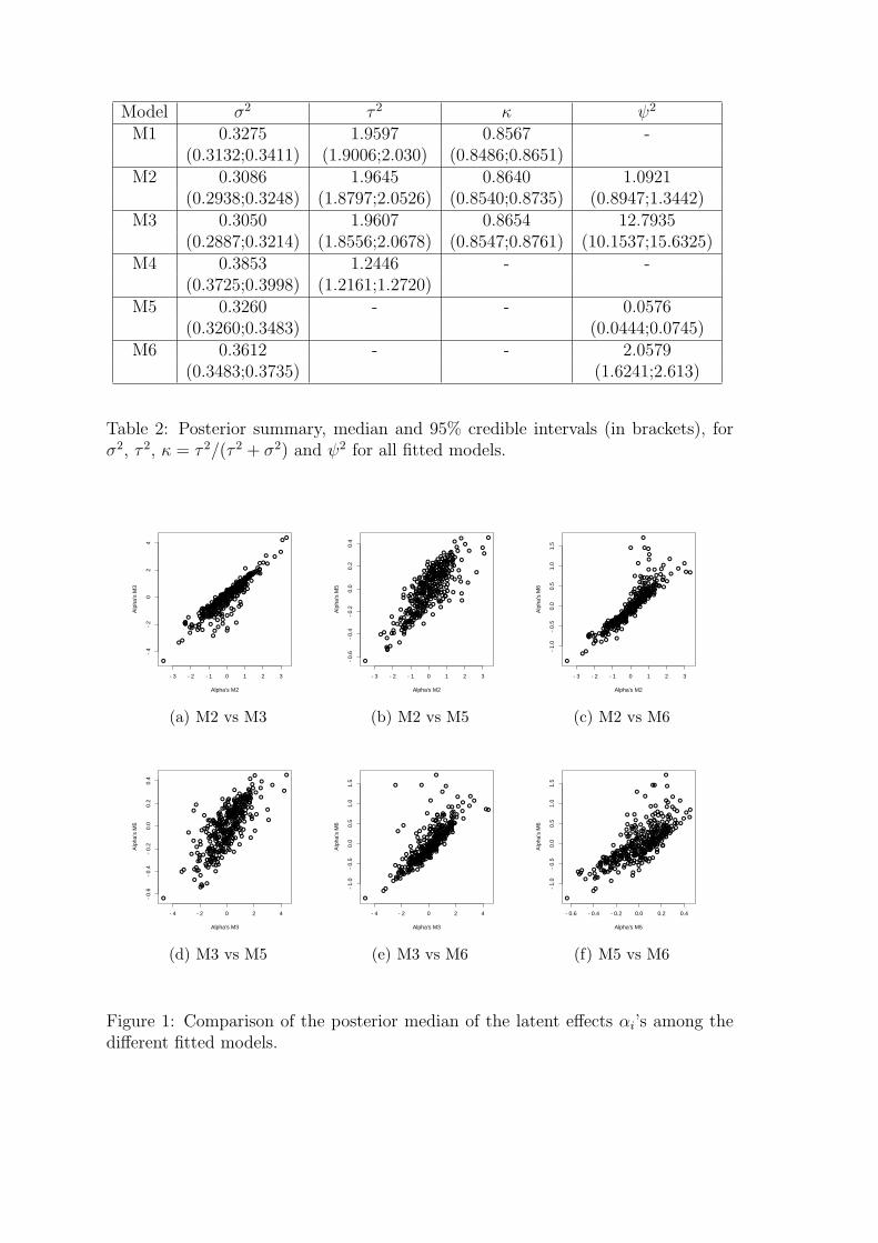
In Table 2, we present the posterior summary of the sources of variability for thedifferent components of the model in (1). That is of σ2, τ 2, the ratio κ = τ 2/(τ 2+σ2)(only when the inneficiencies follow a truncated normal distribution) and ψ2. Asdescribed in Section 3, ψ2, the variance of αi, does not have a straight forwardinterpretation when the CAR prior is assumed. We notice that σ2, the variance ofthe white noise, is the smallest forM3, which is in agreement with EPD and DIC. Wealso notice that κ is relatively big, supporting the inclusion of the inefficiency term

3See http://www.doornik.com/ox/ for more details.

to model this dataset. It is worth mentioning that under M4, τ 2, as reported there,is the mean of the exponential distribution of uij. We do not show the summary ofτ 2 for M5 and M6 as in these cases, the mean of the exponential varies across themunicipalities.

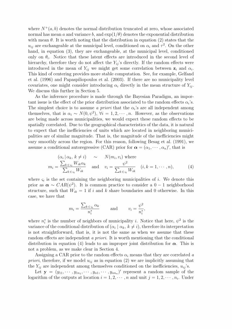
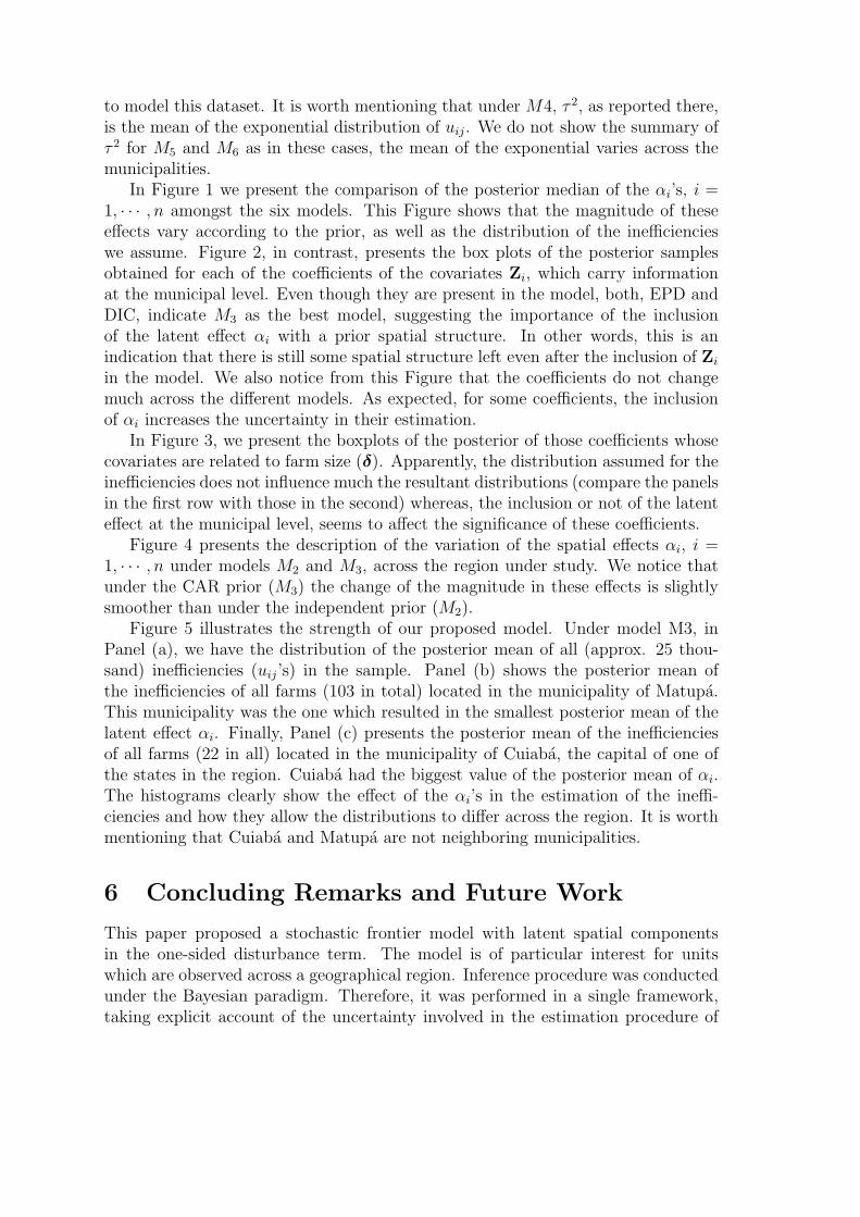
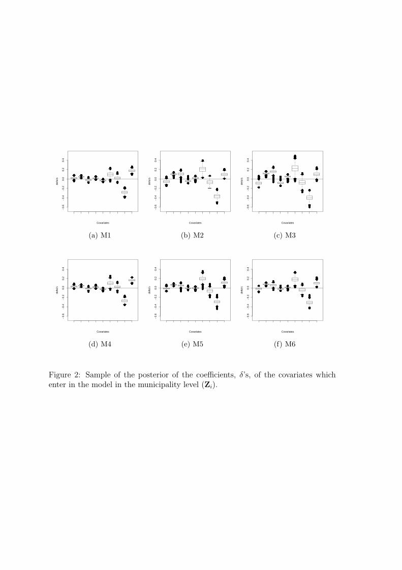
In Figure 1 we present the comparison of the posterior median of the αi’s, i =1, · · · , n amongst the six models. This Figure shows that the magnitude of theseeffects vary according to the prior, as well as the distribution of the inefficiencieswe assume. Figure 2, in contrast, presents the box plots of the posterior samplesobtained for each of the coefficients of the covariates Zi, which carry informationat the municipal level. Even though they are present in the model, both, EPD andDIC, indicate M3 as the best model, suggesting the importance of the inclusionof the latent effect αi with a prior spatial structure. In other words, this is anindication that there is still some spatial structure left even after the inclusion of Zi

in the model. We also notice from this Figure that the coefficients do not changemuch across the different models. As expected, for some coefficients, the inclusionof αi increases the uncertainty in their estimation.

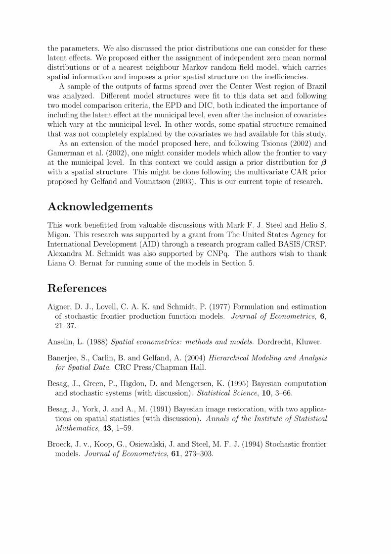
In Figure 3, we present the boxplots of the posterior of those coefficients whosecovariates are related to farm size (δ). Apparently, the distribution assumed for theinefficiencies does not influence much the resultant distributions (compare the panelsin the first row with those in the second) whereas, the inclusion or not of the latenteffect at the municipal level, seems to affect the significance of these coefficients.

Figure 4 presents the description of the variation of the spatial effects αi, i =1, · · · , n under models M2 and M3, across the region under study. We notice thatunder the CAR prior (M3) the change of the magnitude in these effects is slightlysmoother than under the independent prior (M2).

Figure 5 illustrates the strength of our proposed model. Under model M3, inPanel (a), we have the distribution of the posterior mean of all (approx. 25 thou-sand) inefficiencies (uij’s) in the sample. Panel (b) shows the posterior mean ofthe inefficiencies of all farms (103 in total) located in the municipality of Matupa.This municipality was the one which resulted in the smallest posterior mean of thelatent effect αi. Finally, Panel (c) presents the posterior mean of the inefficienciesof all farms (22 in all) located in the municipality of Cuiaba, the capital of one ofthe states in the region. Cuiaba had the biggest value of the posterior mean of αi.The histograms clearly show the effect of the αi’s in the estimation of the ineffi-ciencies and how they allow the distributions to differ across the region. It is worthmentioning that Cuiaba and Matupa are not neighboring municipalities.

6 Concluding Remarks and Future Work

This paper proposed a stochastic frontier model with latent spatial componentsin the one-sided disturbance term. The model is of particular interest for unitswhich are observed across a geographical region. Inference procedure was conductedunder the Bayesian paradigm. Therefore, it was performed in a single framework,taking explicit account of the uncertainty involved in the estimation procedure of

the parameters. We also discussed the prior distributions one can consider for theselatent effects. We proposed either the assignment of independent zero mean normaldistributions or of a nearest neighbour Markov random field model, which carriesspatial information and imposes a prior spatial structure on the inefficiencies.

A sample of the outputs of farms spread over the Center West region of Brazilwas analyzed. Different model structures were fit to this data set and followingtwo model comparison criteria, the EPD and DIC, both indicated the importance ofincluding the latent effect at the municipal level, even after the inclusion of covariateswhich vary at the municipal level. In other words, some spatial structure remainedthat was not completely explained by the covariates we had available for this study.

As an extension of the model proposed here, and following Tsionas (2002) andGamerman et al. (2002), one might consider models which allow the frontier to varyat the municipal level. In this context we could assign a prior distribution for βwith a spatial structure. This might be done following the multivariate CAR priorproposed by Gelfand and Vounatsou (2003). This is our current topic of research.

Acknowledgements

This work benefitted from valuable discussions with Mark F. J. Steel and Helio S.Migon. This research was supported by a grant from The United States Agency forInternational Development (AID) through a research program called BASIS/CRSP.Alexandra M. Schmidt was also supported by CNPq. The authors wish to thankLiana O. Bernat for running some of the models in Section 5.

References

Aigner, D. J., Lovell, C. A. K. and Schmidt, P. (1977) Formulation and estimationof stochastic frontier production function models. Journal of Econometrics, 6,21–37.

Anselin, L. (1988) Spatial econometrics: methods and models. Dordrecht, Kluwer.

Banerjee, S., Carlin, B. and Gelfand, A. (2004) Hierarchical Modeling and Analysisfor Spatial Data. CRC Press/Chapman Hall.

Besag, J., Green, P., Higdon, D. and Mengersen, K. (1995) Bayesian computationand stochastic systems (with discussion). Statistical Science, 10, 3–66.

Besag, J., York, J. and A., M. (1991) Bayesian image restoration, with two applica-tions on spatial statistics (with discussion). Annals of the Institute of StatisticalMathematics, 43, 1–59.

Broeck, J. v., Koop, G., Osiewalski, J. and Steel, M. F. J. (1994) Stochastic frontiermodels. Journal of Econometrics, 61, 273–303.

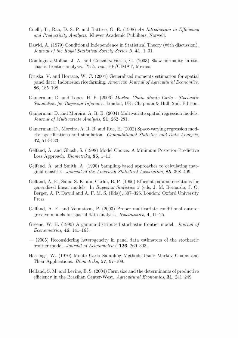
Coelli, T., Rao, D. S. P. and Battese, G. E. (1998) An Introduction to Efficiencyand Productivity Analysis. Kluwer Academic Publihers, Norwell.

Dawid, A. (1979) Conditional Independence in Statistical Theory (with discussion).Journal of the Royal Statistical Society Series B, 41, 1–31.

Domınguez-Molina, J. A. and Gonzalez-Farıas, G. (2003) Skew-normality in sto-chastic frontier analysis. Tech. rep., PE/CIMAT, Mexico.

Druska, V. and Horrace, W. C. (2004) Generalized moments estimation for spatialpanel data: Indonesian rice farming. American Journal of Agricultural Economics,86, 185–198.

Gamerman, D. and Lopes, H. F. (2006) Markov Chain Monte Carlo - StochasticSimulation for Bayesian Inference. London, UK: Chapman & Hall, 2nd. Edition.

Gamerman, D. and Moreira, A. R. B. (2004) Multivariate spatial regression models.Journal of Multivariate Analysis, 91, 262–281.

Gamerman, D., Moreira, A. R. B. and Rue, H. (2002) Space-varying regression mod-els: specifications and simulation. Computational Statistics and Data Analysis,42, 513–533.

Gelfand, A. and Ghosh, S. (1998) Model Choice: A Minimum Posterior PredictiveLoss Approach. Biometrika, 85, 1–11.

Gelfand, A. and Smith, A. (1990) Sampling-based approaches to calculating mar-ginal densities. Journal of the American Statistical Association, 85, 398–409.

Gelfand, A. E., Sahu, S. K. and Carlin, B. P. (1996) Efficient parameterizations forgeneralised linear models. In Bayesian Statistics 5 (eds. J. M. Bernardo, J. O.Berger, A. P. Dawid and A. F. M. S. (Eds)), 307–326. London: Oxford UniversityPress.

Gelfand, A. E. and Vounatsou, P. (2003) Proper multivariate conditional autore-gressive models for spatial data analysis. Biostatistics, 4, 11–25.

Greene, W. H. (1990) A gamma-distributed stochastic frontier model. Journal ofEconometrics, 46, 141–163.

— (2005) Reconsidering heterogeneity in panel data estimators of the stochasticfrontier model. Journal of Econometrics, 126, 269–303.

Hastings, W. (1970) Monte Carlo Sampling Methods Using Markov Chains andTheir Applications. Biometrika, 57, 97–109.

Helfand, S. M. and Levine, E. S. (2004) Farm size and the determinants of productiveefficiency in the Brazilian Center-West. Agricultural Economics, 31, 241–249.

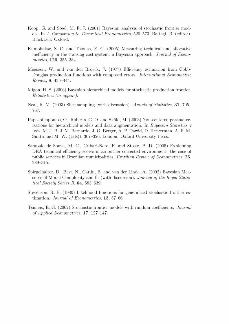
Koop, G. and Steel, M. F. J. (2001) Bayesian analysis of stochastic frontier mod-els. In A Companion to Theoretical Econometrics, 520–573. Baltagi, B. (editor).Blackwell: Oxford.

Kumbhakar, S. C. and Tsionas, E. G. (2005) Measuring technical and allocativeinefficiency in the translog cost system: a Bayesian approach. Journal of Econo-metrics, 126, 355–384.

Meeusen, W. and van den Broeck, J. (1977) Efficiency estimation from Cobb-Douglas production functions with composed errors. International EconometricReview, 8, 435–444.

Migon, H. S. (2006) Bayesian hierarchical models for stochastic production frontier.Estadistica (to appear).

Neal, R. M. (2003) Slice sampling (with discussion). Annals of Statistics, 31, 705–767.

Papaspiliopoulos, O., Roberts, G. O. and Skold, M. (2003) Non-centered parameter-isations for hierarchical models and data augmentation. In Bayesian Statistics 7(eds. M. J. B. J. M. Bernardo, J. O. Berger, A. P. Dawid, D. Heckerman, A. F. M.Smith and M. W. (Eds)), 307–326. London: Oxford University Press.

Sampaio de Souza, M. C., Cribari-Neto, F. and Stosic, B. D. (2005) ExplainingDEA technical efficiency scores in an outlier corrected environment: the case ofpublic services in Brazilian municipalities. Brazilian Review of Econometrics, 25,289–315.

Spiegelhalter, D., Best, N., Carlin, B. and van der Linde, A. (2002) Bayesian Mea-sures of Model Complexity and fit (with discussion). Journal of the Royal Statis-tical Society Series B, 64, 583–639.

Stevenson, R. E. (1980) Likelihood functions for generalized stochastic frontier es-timation. Journal of Econometrics, 13, 57–66.

Tsionas, E. G. (2002) Stochastic frontier models with random coefficients. Journalof Applied Econometrics, 17, 127–147.

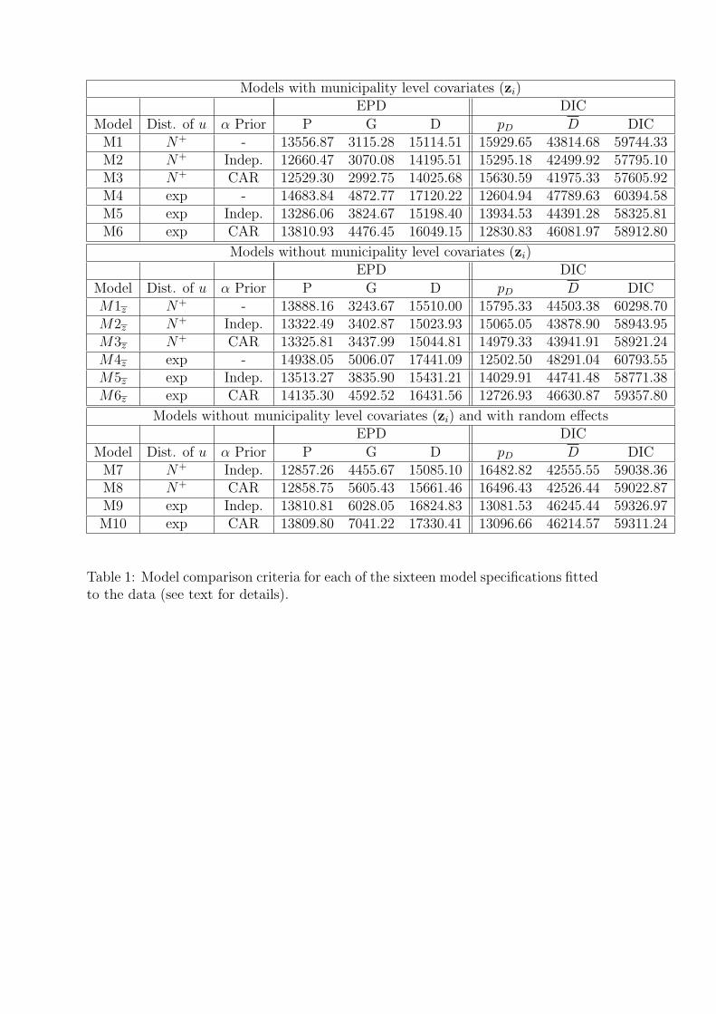
Models with municipality level covariates (zi)EPD DIC

Model Dist. of u α Prior P G D pD D DICM1 N+ - 13556.87 3115.28 15114.51 15929.65 43814.68 59744.33M2 N+ Indep. 12660.47 3070.08 14195.51 15295.18 42499.92 57795.10M3 N+ CAR 12529.30 2992.75 14025.68 15630.59 41975.33 57605.92M4 exp - 14683.84 4872.77 17120.22 12604.94 47789.63 60394.58M5 exp Indep. 13286.06 3824.67 15198.40 13934.53 44391.28 58325.81M6 exp CAR 13810.93 4476.45 16049.15 12830.83 46081.97 58912.80

Models without municipality level covariates (zi)EPD DIC

Model Dist. of u α Prior P G D pD D DICM1z N+ - 13888.16 3243.67 15510.00 15795.33 44503.38 60298.70M2z N+ Indep. 13322.49 3402.87 15023.93 15065.05 43878.90 58943.95M3z N+ CAR 13325.81 3437.99 15044.81 14979.33 43941.91 58921.24M4z exp - 14938.05 5006.07 17441.09 12502.50 48291.04 60793.55M5z exp Indep. 13513.27 3835.90 15431.21 14029.91 44741.48 58771.38M6z exp CAR 14135.30 4592.52 16431.56 12726.93 46630.87 59357.80

Models without municipality level covariates (zi) and with random effectsEPD DIC

Model Dist. of u α Prior P G D pD D DICM7 N+ Indep. 12857.26 4455.67 15085.10 16482.82 42555.55 59038.36M8 N+ CAR 12858.75 5605.43 15661.46 16496.43 42526.44 59022.87M9 exp Indep. 13810.81 6028.05 16824.83 13081.53 46245.44 59326.97M10 exp CAR 13809.80 7041.22 17330.41 13096.66 46214.57 59311.24

Table 1: Model comparison criteria for each of the sixteen model specifications fittedto the data (see text for details).

Model σ2 τ 2 κ ψ2

M1 0.3275 1.9597 0.8567 -(0.3132;0.3411) (1.9006;2.030) (0.8486;0.8651)

M2 0.3086 1.9645 0.8640 1.0921(0.2938;0.3248) (1.8797;2.0526) (0.8540;0.8735) (0.8947;1.3442)

M3 0.3050 1.9607 0.8654 12.7935(0.2887;0.3214) (1.8556;2.0678) (0.8547;0.8761) (10.1537;15.6325)

M4 0.3853 1.2446 - -(0.3725;0.3998) (1.2161;1.2720)

M5 0.3260 - - 0.0576(0.3260;0.3483) (0.0444;0.0745)

M6 0.3612 - - 2.0579(0.3483;0.3735) (1.6241;2.613)

Table 2: Posterior summary, median and 95% credible intervals (in brackets), forσ2, τ 2, κ = τ 2/(τ 2 + σ2) and ψ2 for all fitted models.

●

●

●

●●

●●

●●

●

●

●

●

●

●

●

●

●●

●

●

●

●

●

●●●

●

●

●●

●

●

●

●

●

●

●

●

●

●

●

●●

●●

●

●

●●

●

●

●

●

●

●

●

●

●

●

●

●

●

●

●

●

●

●

●●

●

●

●●

●

●

●

●

●

●

●

●

●●

●●

●

●

●●

●

●

●

●

●

●

●

●

●

●

●

●

●

●●

●●

●

●●

●

●

●

●

●

●

●

●

●

●

●

●

●

●

●

●

●

●●

●

●

●

●

●

●●

●●

●

●

●

●

●

●

●

●

●●

●

●

●

●

●●

●

● ●

●

●●

●

●●

●

●●●

●●

●

●

●

●

●

●

●

●

●

●

●

●

●

●

●

●

●

●

●

●

●●

●●

●

●

●

●

●

●●

●

●

●

●

●

●

●

●

●

●●

●

●●●●

●

●

●

●

●

●

●

●

●

●

●

● ●●●

●

●

●

●

●

●

●

●

●

●●

●

●●

●

●

●●

●

●

●

●

●

●

●

●●

●

●

●●

●

●●

●

●

●

●

●

●

●

●

●

●

●

●

●

●

●

●

●

●

●●

●

●

●

●●

●●● ●

●

●

●

●●

●

●

●

●

●

●

●

●●

●

●

●

●

●

●●

●

●

●●

●

●

●

●

●●

●

●

●

●●●

●

●●

●

●

●

●

●

●●

●

●

●

●

●

●

●

●●

●

●●●

●

●

●

●

●

●

●

●

●

●

●

●

●

●

●

●

−3 −2 −1 0 1 2 3

−4

−2

02

4

Alpha’s M2

Alp

ha’s

M3

(a) M2 vs M3

●●

●●

●

●●

●

● ●●

●

●

●

●

●

●

●●

●●

●

●

●●

●

●

●

●

●

●

●

●

●

●

●

●

●●

●

●

●●

●

●

●

●

●●

● ●

●●

●

●

●

●

●

●●

●

●

●●

●

●

●

●

●

●

●

●

●

●

●

●

●

●●

●

●

●

●

●

●

●

●

●

●

● ●

●

●

●

●

●●

●

●

●●

●

●

●

●

●

●

●

●

●

● ●

●●

●

●

●

●

●●

●

●

●

●

●

●

●●

●

●

●

●

●

●

●

●

●●

● ●

●

●

●

●

●

●

●

●

●

●

●

●

●●

●

●

●

●

●

●

●●

●

●

●●

●

●●

● ●

●

●

●

●

●

●

●

●

●

●

●

●

●

●

●

●

●

●

●

●

●

●

●

●

●●

●

●

●●

●

● ●

●

●

●

●

●

●

●

●

●

●

●

●

●

●

●

●

●

●

●

●

●

●

●

●

●●

●

●

●

●

●

●●

●

●

●

●

●●

●

●

●

●●

●

●

●

●

●

●

●

●

●

●

●●

● ●

●

●

●

●

●

●●

●

●

●

●

●

●

●

●

●

●

●

●

●

●

●

●

●

●

●

●

●

●

●

●

● ●

●

●●

●

●

●●

●

●

●

●

● ●

●

●

●

●

●

●

●

●

●

●

●

●

●

●

●

●

●

●

●

●

●●

●

●

●●

●

●

●

●

●●

●

●

●

●

●

●

●

●

●●

●

●●●

●

●

●

●

●

●

● ●

●

●

●

●

●

●

●

●

−3 −2 −1 0 1 2 3

−0.

6−

0.4

−0.

20.

00.

20.

4

Alpha’s M2

Alp

ha’s

M5

(b) M2 vs M5

● ●

●

●●

●

●

●●●

●

●

●

●●●

●

●●

●

●

●●

●

●

●

●

●

●●

●

●

●

●

●●

●

●

●

●

●

●

●

●

●

●

●

●

●

● ●

●

●

●

●

●

●

●

●

●

●

●

●

●

●

●●

●

●●

●

●

●

●

●

●

●

●

●

●

●

●

●

●

●

●

●

●

●

● ●

●

●

●

●

●

●

●

●

●

●

●

●

●●

●●

●

●●

●

●

●

●

●

●

●

●

●

●

●

●

●

●

●

●

●

●●●

●

●

●

●●

●

●●

●

●

●

●

●

●

●

●

●●

●

●●

●

●

●

●

●●

●

●●

●

●

●

●

●●●

●●

●

●

●

●

●

●

●

●

●

●

●●

●

●

●

●

●

●

●

●

●

●

●

●

●

●

●

●

●

● ●

●

●

●●

●

●

●

●

●

●

●

●

●

●●●●●

●

●

●

●

●

●

●●

●

● ●●

●

●

●

●●

●

●

●

●

●

●●●

●●

●

●

●

●

●

●

●●

●

●

●

●

●

●

●

●

●

●

●●

●

●

●

●

●●●

●

●

●

●

●

●

●

●

●

●●

●●

●

●

●

●

●

●

● ●

●

●

●

●

●●

●

●

●

●

●

●

●

●

●

●

●●

●

●

●

●

●●

●

●

● ●

●

●

●

●

●

●

●

●

●●●

●●

●

●●

●●

●

●

●

●

●● ●

●

●

●●

●

●●●

●

●

●

●

●

●

●

● ●

●

●

●

●●

●

●

−3 −2 −1 0 1 2 3

−1.

0−

0.5

0.0

0.5

1.0

1.5

Alpha’s M2

Alp

ha’s

M6

(c) M2 vs M6

●●

●●

●

●●

●

● ●●

●

●

●

●

●

●

●●

●●

●

●

●●

●

●

●

●

●

●

●

●

●

●

●

●

●●

●

●

● ●

●

●

●

●

●●

● ●

●●

●

●

●

●

●

●●

●

●

●●

●

●

●

●

●

●

●

●

●

●

●

●

●

●●

●

●

●

●

●

●

●

●

●

●

● ●

●

●

●

●

●●

●

●

●●

●

●

●

●

●

●

●

●

●

● ●

● ●

●

●

●

●

●●

●

●

●

●

●

●

●●

●

●

●

●

●

●

●

●

●●

● ●

●

●

●

●

●

●

●

●

●

●

●

●

●●

●

●

●

●

●

●

●●

●

●

●●

●

●●

● ●

●

●

●

●

●

●

●

●

●

●

●

●

●

●

●

●

●

●

●

●

●

●

●

●

●●

●

●

●●

●

● ●

●

●

●

●

●

●

●

●

●

●

●

●

●

●

●

●

●

●

●

●

●

●

●

●

●●

●

●

●

●

●

●●

●

●

●

●

●●

●

●

●

●●

●

●

●

●

●

●

●

●

●

●

●●

●●

●

●

●

●

●

●●

●

●

●

●

●

●

●

●

●

●

●

●

●

●

●

●

●

●

●

●

●

●

●

●

● ●

●

●●

●

●

●●

●

●

●

●

●●

●

●

●

●

●

●

●

●

●

●

●

●

●

●

●

●

●

●

●

●

●●

●

●

●●

●

●

●

●

●●

●

●

●

●

●

●

●

●

●●

●

●●●

●

●

●

●

●

●

●●

●

●

●

●

●

●

●

●

−4 −2 0 2 4

−0.

6−

0.4

−0.

20.

00.

20.

4

Alpha’s M3

Alp

ha’s

M5

(d) M3 vs M5

● ●

●

●●

●

●

●●●

●

●

●

●●●

●

●●

●

●

●●

●

●

●

●

●

●●

●

●

●

●

●●

●

●

●

●

●

●

●

●

●

●

●

●

●

● ●

●

●

●

●

●

●

●

●

●

●

●

●

●

●

●●

●

●●

●

●

●

●

●

●

●

●

●

●

●

●

●

●

●

●

●

●

●

● ●

●

●

●

●

●

●

●

●

●

●

●

●

●●

●●

●

●●

●

●

●

●

●

●

●

●

●

●

●

●

●

●

●

●

●

●● ●

●

●

●

●●

●

●●

●

●

●

●

●

●

●

●

●●

●

●●

●

●

●

●

●●

●

●●

●

●

●

●

●●●

●●

●

●

●

●

●

●

●

●

●

●

●●

●

●

●

●

●

●

●

●

●

●

●

●

●

●

●

●

●

●●

●

●

●●

●

●

●

●

●

●

●

●

●

●●● ●●

●

●

●

●

●

●

●●

●

●●●

●

●

●

●●

●

●

●

●

●

●●●

●●

●

●

●

●

●

●

●●

●

●

●

●

●

●

●

●

●

●

●●

●

●

●

●

●● ●

●

●

●

●

●

●

●

●

●

● ●

●●

●

●

●

●

●

●

● ●

●

●

●

●

●●

●

●

●

●

●

●

●

●

●

●

●●

●

●

●

●

●●

●

●

● ●

●

●

●

●

●

●

●

●

●●●

●●

●

●●

● ●

●

●

●

●

●● ●

●

●

●●

●

●●●

●

●

●

●

●

●

●

● ●

●

●

●

● ●

●

●

−4 −2 0 2 4

−1.

0−

0.5

0.0

0.5

1.0

1.5

Alpha’s M3

Alp

ha’s

M6

(e) M3 vs M6

●●

●

●●

●

●

● ●●

●

●

●

●●●

●

●●

●

●

●●

●

●

●

●

●

●●

●

●

●

●

●●

●

●

●

●

●

●

●

●

●

●

●

●

●

●●

●

●

●

●

●

●

●

●

●

●

●

●

●

●

●●

●

●●

●

●

●

●

●

●

●

●

●

●

●

●

●

●

●

●

●

●

●

●●

●

●

●

●

●

●

●

●

●

●

●

●

● ●

●●

●

●●

●

●

●

●

●

●

●

●

●

●

●

●

●

●

●

●

●

●● ●

●

●

●

●●

●

●●

●

●

●

●

●

●

●

●

●●

●

●●

●

●

●

●

●●

●

●●

●

●

●

●

●● ●

●●

●

●

●

●

●

●

●

●

●

●

●●

●

●

●

●

●

●

●

●

●

●

●

●

●

●

●

●

●

●●

●

●

●●

●

●

●

●

●

●

●

●

●

●●● ●●

●

●

●

●

●

●

●●

●

● ●●

●

●

●

●●

●

●

●

●

●

●●●

● ●

●

●

●

●

●

●

●●

●

●

●

●

●

●

●

●

●

●

● ●

●

●

●

●

●●●

●

●

●

●

●

●

●

●

●

● ●

● ●

●

●

●

●

●

●

● ●

●

●

●

●

●●

●

●

●

●

●

●

●

●

●

●

●●

●

●

●

●

●●

●

●

● ●

●

●

●

●

●

●

●

●

● ●●

●●

●

●●

●●

●

●

●

●

●● ●

●

●

●●

●

● ●●

●

●

●

●

●

●

●

● ●

●

●

●

● ●

●

●

−0.6 −0.4 −0.2 0.0 0.2 0.4

−1.

0−

0.5

0.0

0.5

1.0

1.5

Alpha’s M5

Alp

ha’s

M6

(f) M5 vs M6

Figure 1: Comparison of the posterior median of the latent effects αi’s among thedifferent fitted models.

●●●●●●●●●●●●●●●●●●●●●●●●●●●●●●●●●●●●●●●●●●●●●●●●●●●●●●●●●●●●●●●●●●●●●●●●●●●●●●●●●●●●●●●●●●●●●●●●●●●●●●●●●●●●●●●●●●●●●●●●●●●●●●●●●●●●●●●●●●●●●●●●●●●●●●●●●●●●●●●●●●●●●●

●●●●●●●●

●●●●●●●●●●●●●●●●●●●●●●●●●●●●●●●●●●●●●●●●●●●●●●●●●●●●●●●●●●●●●●●●●●●●●●●●●●●●●●●●●●●●●●●●●●●●●●●●●●●●●●●●●●●●●●●●●●●●●●●●●●●●●●●●●●●●●●●●●●●●●●●●●●●●●●●●●●●●●●●●●●●●●●●●●●●●●●●●●●●●●●●●●●●●●●●●●●●●●●●●●●●●●●●●●

●●●●●●●●●●●●●●●●●●●●●●●●●●●●●●●●●

●

●●●●●●●●●●●●●●●●●●●

●●●●●●●●●●●●●●

●●●●●●●●●●●●●●●●●●●●●●●●●●●●●●●●●●●●●●●●●●●●

●●●●●●●●●●●●●●●●●●●●●●●●●●●

●●●●●●●

●●●●●●●●

●●●●●●●●●●●●●●●●●●●●●●●●●●●●●●●●●●●●●●●●●●●●●●●●●●●●●●●●●●

●

●●●●●●●

●●●●●●●●●●●●●●●●●●●●●●●●●●●●●●●●●●●●●●●●●●●●●●●●●●●●●●●●●●●●●●●

●●●●●●●●●●●●●●●●●●●●●●●●●●●●●●●●●●●●●●●●●●●●●●●

●●●●●●●●●●●●●●●●●●●●●●●●●●

●●●●●●●●●●●

●

●●●●●●●●●●●●●●●●●●●●●●●●●●●●●●●●●●●●●●●●●●●●●●●●●●●●●●●●●●●●●●●●●●●●●●●●●●●

●●●●●●●●●●●●●●●●●●●●●●●●●●●●●●●●●●●●●●●●●●●●●●●●●●●●●●●●●●●●●●●●●●●●●●●●●●●●●●●●●●●●●●●●●●●●●●●●●●●●●●●●●●●●●●●●●●●●●●●●●●●●●●●●●●●●●●●●●●●●●●●●●●●●●●●●●●●●●●●●●●●●●●●●●●●●●●●●●●●●●●●●●●●●●●●●●●●●●●●●●

●●●

●●●●●●●●●●●●●●●●●●●●●●●●●●●●●●●●●●●●

●●●

●●

●●●●●●●

●●●

●

●●●●●●

●●●●●●●●●●●●●●●●●●●●●●●●●●●●●●●●●●●●●●●●●●●●●●●●●●●●●●●●●●●●●●●●●●●●●●●●●●●●●●●●●●●●●●●●●●●●●●●●●●●●●●●●●●●●●●●

●●

●●●●●●●●●●●●●●●●●●●●●●●●●●●●●●

●●●●●●●●●●●●●●●●●●●●●●●●●●●●●●●●●●●●●●●●●●●●●●●

●●●●●●●●●●●●●●

●●●●●●●●●●●●●●●●●●●●●●●●●●●●●●●●●●●●●●●●●●●●●●●●●●●●●●●●

●●●●●●●●●●●●●●●●●●●●●

●●●

●●●●●●●●●●●●●●●●●●●●●●●●●●●●●●●●●●●●●

●●●●●●●●●●●●●●●●●●●●●●●●●●●●●●●●●

●●●●●●●

●●●●●●●●●●●●●●●●●●●●●●●●●●●●●●●●●

●●●●●●●●●●●●●●●●●●●●●●●●●●●●●●●●●●●●●●●

●●●●●●●●●●●●●●●●●●●●●●●●●●●●●●●●●●●●●●●●●●●●●●●●●●●●●●●●●●●●●●●●●●

●●●●●●●●●●●●●●●●●●●●●●●●●●●●●●●●●●●●●●●●●●●●●●●●●●

●●●●●●●●●●●●●●●

●●●●●●●●●●●●●●●●

●

●●●●●●●●●●●●●●●●

●●●●●●●

●●●●●●●●●●●●●●●●●●●●●●●●●●●●●●●●●●●●●●●●●●●●●●●●●●●●●●●●●●●●●●●●●●●●●●●●●●●●●●●●●●●●●●●●●●●●●●●●●●●●●●●●●●●●●●●●●●●●●●●●●●●

●●●●●●●●

●●●●●●●●●●●●●●●●●●●●●●●●●●●●●●●●●●●●●●●●●●●●●●●●●●●●●●●●●●●●●●●●●●●●●●●●●●●●●●●●●●

●●●●●●●●

●●●●

●●●●●●●●●●●●●●●●●●●●●●●●

●●●●●●●●●

●●●●●●●●●●●●

●●●●●

●●●●●●●●●●●●●●●●●●●●●●●●●●●●●●●●●●●●●●●●●●

●●●●●●●●●●●●●●●●●●●●●●●

●●●●●●●●●●●●●●●●●●●●●●●●●●●●●●●●●●●●●●●●●●●●●●●●●●●●●●●●●●●●●●●●●●●●●●●●●●●●●●●●●●●●●●●●●●

●●●●

●●●●●●●●●●●●●●●●●●●●●●●●●●●●●●●●●●●●●●●●●●●●●●●●●●●●●●●●●●●●●●●●●●

●

●●●●●●●●●

●●

●●●●●●●●●●●●

●●●●●●●●●●●●●●●●●●●●●●●●●●●●●●●●●●●●●●●●●●●●●●●●●●●●●●●●●●●●●●●●

●●●

●●●●●●●●●●●●●●●●●●●●●●●●●●●●●●●●

●●●●●●●●●●●●●●●●●●●●●●●●●●●●●●●●●●●●●●●●●●●●●●●●●●●●●●●●●●●●●●●●●●●●●●●●●●●●●●●●●●●●●●●●●●●●●●●●●●●●●●●●●●●●●●●●●

●●●

●●●●●●●●●●●●●●●●●●●●●●●●●●●●●●●●●●●●●●●●●●●●●●●●●●●●●●●●●●●●●●●●●●●●●●●●●●●●●●●●●●●●●●●●●●●●●●●●●●

●●●●●●●●●●●●●●●●●●●●●●●●●●●●●

●●●●●●●●

●●●●●●●●●●

●●●●●●●●●●●●●●●●●●●●●

●

●●●●●●●●●●●●●●●●●●

●●●●●●●●●●●●●●●●

●●●●●●●●●●●●●●●●●●●●●●

●

●

●

●●

●●●●●●●●●●●●●●●●●●●●●●●●●●●●●●●●●●●●●●●●●●●●●●●●●●●●●●●●●●●●●●●●●●●●●●●●

●●●●●●●

●●●●●●●●●●●●●●●●●●●●●●●●●●●●●●●●●●●●●●●●●●●●●●●●●●●●●●●●●●●●●●●●

●●●●

●●●●●●●●●●●●●●●●●●●●●●●●●●

●●●●●●●●

●●●●●●●●●●●●●●●●●●●●

●●●●●●●●

●●●●

●●●●●●●●●

●●●●●●●●

●●●●●●●●●●●●●●●●●●●●●●●●

●●●●●●●●●●●●●●●●●●●●●●●●●●●●●●●●●●●●●

●●●●●●●●●●●●●●●●●●●●●●●●●●●●●●●●●●●●●●●●●●●●●●●●

●●

●●●●●●●●●●●●●●

●●●●●●●●●●●●●●●●●●●●●●●●●●●●●●●●●●●●●●●●●●●●●●

●●●●●●●●●●●●●●●●●●●●●●●●●●

●●●●●●●●●●●●●●●●●●●●●●●

●●●●●●●●●●●●●●●●●●●●●●●●●●●●●●●●●

●●●●●●●●●●●●●●●●●●●

●●

●●

●●●●●

●●●●●●●

●●●

●●●●●●●●●●●●●●●●●●●●●●●●●●●●●●●●●●●●●●●●●●●●●●

●●●●●●●●●●●●●●●●●●●●●●●●●●●●●●●●●●●●●●●●●●●●●●●●●●●●●●●●●●●●●●●●●●●●●●●●●●●●●●●●●●●●●●●●●●●●●●●●●●●●●●●●●●●●●●●●●●●●●●●●●●●●●●●●●●●●●●●●●●●●●●●●●●●●●●●●●●●●●●●●●●●●●●●●

●●●●●●●●●●●●●●●●●●●●●●●●●●●●●●●●●●●●●●●●

●●●●●●●●●●●●●

●●●●●●

●●●●●●●●●●●●●●●●●●●●●●●●●●●●●●●●●●●●●●●●●●●●●●●●●●●●●●●●●●●●●●●●●●●●●●●●●●●●●●●●●●●●●●●●●●●●●●●●●●

●●●●●●●●●●●●●●●●●

−0.

6−

0.4

−0.

20.

00.

20.

4

Covariates

delta

’s

(a) M1

●●●●●●●●●●●●●●●●●●●●●●●●●●●●●●●●●●●●●●●●●●●●●●●●●●●●●●●●●●●●●●●●●●●●●●●●●●●●●●●●●●●●●●●●●●●●●●●●●●●●●●●●●●●●●●●●●●●●●●●●●●●●●●●●●●●●●●●●●●●●●●●●●●●●●●●●●●●●●●●●●●●●●●●●●●●●●●●●●●●●●●●●●●●●●●●●●●●●●●●●●●●●●●●●●●●●●●●●●●●●●●●●●●●●●●●●●●●●●●●●●●●●●●●●●●●●●●●●●●●●●●●●●●●●●●●●●●●●●●●●●●●●●●●●●●●●●●●●●●●●

●●●●●●●●●●●●●●●●●●●●●●●●●●●●●●●●●●●●●●●●●●●●●●●●●●●●●●●●●●●●●●●●●●●●●●●●●●●●●●●●●●●●●●●●●●●●●●●●●●●●●●●●●●●●●●●●●●●●●●●●●●●●●●●●●●●●●●●●●●●●●●●●●●●●●●●●●●●●●●●●●●●●●●●●●●●●●●●●●

●●●●●●●

●●●●●●●●●●●●●●●●●●●●●●●●●●●●●●●●

●●●●●●●●●●●●●●●●●●●●●●●●●●●●●●●●●●●●●●●●●●●●●●●●●●●●●●●●●●●●●●●●●●●●●●●●●●●●●●●●●●●●●●●●●●●●●●●●●●●●●●●●●●●●●●●●●●●●●●●●●●●●●●●●●●●●●●●●●●●●●●●●●●●●●●●●●●●●●●●●●●●●●●●●●●●●●●●●●●●●●●●●●●●●●●●●●●●●●●●●●●●●●●●●●●●●●●●●●●●●●●●●●●●●●●●●●●●●●●●●●●●●●●●●●●●●●●●●●●●●●●●●●●●●●●●●●●●●●●●●●●●●●●●●●●●●●●●●●●●●●●●●●●●●●●●●●●●●●●●●●●●●●●●●●●●●●●●●●●●●●●●●●●●●●●●●●●●●●●●●●●●●●●●●●●●●●●●●●●●●●●●●●●●●●●●●●●●●●●●●●●●●●●●●●●●●●●●●●●●●●●●●●●●●●●●●●●●●●●●●●●●●●●●●●●●●●●●●●●●●●●●●●●●●●●●●●●●●●●●●●●●●●●

●●●●●●●●●●●●●●●●●●●●●●●●●●●●●●●●●●●●●●●●●●●●●●●●●●●●●●●●●●●●●●●●●●●●●●●●●●●●●●●●●●●●●●●●●●●●●●●●●●●●●●●●●●●●●●●●●●●●●●●●●●●●●●●●●●●●●●●●●●●●●●●●●●●●●●●●●

●●●●●●●●●●●●●●●●●●●●●●●●●●●●●●●●●●●●

●●●●●●●●●●●●●●●●●●●●●●●●●●●●●●●●●●●●●●●●●●●●●●●●●●●●●●●●●●●●●●●●●●●●●●●●●●●●●●●●●●●●●●●●●●●●●●●●●●●●●●●●●●●●●●●●●●●●●●●●●●●●●●●●●●●●●●●●●●●●●●●●●●●●●●●●●●●●●●●●●●●●●●●●●●●●●●●●●●●●●●●●●●●●●●●●●●●●●●●●●●●●●●●●●●●●●●●●●●●●●●●●●●●●●●●●●●●●●●●●●●●●●●●●●●●●●●●●●●●●●●●●●●●●●●●●●●●●●●●●●●●●●●●●●●●●●●●●●●●●●●●●●●●●●●●●●●●●●●●●●●●●●●●●●●●●●●●●●●●●●●●●●●●●●●●●●●●●●●●●●●●●●●●●●●●●●●●●●●●●●●●●●●●●●●●●●●●●●●●●●●●●●●●●●●●●●●●●●●●●●●●●●●●●●●●●●●●●●●●●●●●●●●●●●●●●●●●●●●●●●●●●●●●●●●●●●●●●●●●●●●●●●●●●●●●●●●●●●●●●●●●●●●●●●●●●●●●●●●●●●●●●●●●●●●●●●●●●●●●●●●●●●●●●●●●●●●●●●●●●●●●●●●●●●●●●●●●●●●●●●●●●●●●●●●●●●●●●●●●●●●●●●●●●●●●●●●●●●●●●●●●●●●●●●●●●●●●●●●●●●●●●●●●●●●●●●●●●●●●●●●●●●●

●●●●●●●●●●●●●●●●●●●●●●●●●●●●●●●●●●●●●●●●●●●●●●●●●●●●●●●●●●●●●●●●●●●●●●●●●●●●●●●●●●●●●●●●●●●●●●●●●●●●●●●●●●●●●●●●●●●●●●●●●●●●●●●●●●●●●●●●●●●●●●●●●●●●●●●●●●●●●●●●●●●●●●●●●●●●●●●●●●●●●●●●●●●●●●●●●●●●●●●●●●●●●●●●●●●●●●●●●●●●●●●●●●

●●●●●●●●●●●●●●●●●●●●●●●●●●●●●●●●●●●●●●●●●●●●●●●●●●●●●●●●●●●●●●●●●●●●●●●●●●●●●●●●●●●●●●●●●●●●●●●●●●●●●●●●●●●●●●●●●●●●●●●●●●●●●●●●●●●●●●●●●●●●●●●●●●●●●●●●●●●●●●●●●●●●●●●●●●●●●●●●●●●●●●●●●●●●●●●●●●●●●●●●●●●●●●●●●●●●●●●●●●●●●●●●●●●●●●●●●●●●●●●●●●●●●●●●●●●●●●●●●●●●●●●●●●●●●●●●●●●●●●●●●●●●●●●●●●●●●●●●●●●●●●●●●●●●●●●●●●●●●●●●●●●●●●●●●●●●●●●●●●●●●●●●●●●●●●●●●●●●●●●●●●●●●●●●●●●●●●●●●●●●●●●●●●●●●●●●●●●●●●●●●●●●●●●●●●●●●●●●●●●●●●●●●●●●●●●●●●●●●●●●●●●●●●●●●●●●●●●●●●●●●●●●●●●●●●●●●●●●●●●●●●●●●●●●●●●●●●●●●●●●●●●●●●●●●●●●●●●●●●●●●●●●●●●●●●●●●●●●●●●●●●●●●●●●●●●●●●●●●●●●●●●●●●●●●●●●●●●●●●●●●●●●●●●●●●●●●●●●●●●●●●●●●●●●●●●●●●●●●●●●●●●●●●●●●●●●●●●●●●●●●●●●●●●●●●●●

●●●

●●●●●●●●●●●●●●●●●●●●●●●●●●●●

●●●●●●●●●●●●●●●●●●●●●●●●●●●●●●●●●●●●●●●●●●●●●●●●●●●●●●●●●●●●●●●●●●●●●●●●●●●●●●●●●●●●●●●●●●●●●●●●●●●●●●●●●●●●●●●●●●●●●●●●●●●●●●●●●●●●●●●●●●●●●●●●●●●●●●●●●●●●●●●●●●●●●●●●●●●●●●●●●●●●●●●●●●●●●●●●●●●●●●●●●●●●●●●●●●●●●●●●●●●●●●●●●●●●●●●●●●●●●●●●●●●●●●●●●●●●●●●●●●●●●●●●●●●●●●●●●●●●●●●●●●●●●●●●●●●●●●●●●●●●●●●●●●●●●●●●●●●●●●●●●●●●●●●●●●●●●●●●●●●●●●●●●●●●●●●●●●●●●●●●●●●●●●●●●●●●●●●●●●●●●●●●●●●●●●●●●●●●●●●●●●●●●●●●●●●●●●●●●●●●●●●●●●●●●●●●●●●●●●●●●●●●●●●●●●●●●●●●●●●●●●●●●●●●●●●●●●●●●●●●●●●●●●●●●●●●●●●●●●●●●●●●●●●●●●●●●●●●●●●●●●●●●●●●●●●●●●●●●●●●●●●●●●●●●●●●●●●●●●●●●●●●●●●●●●●●●●●●●●●●●●●●●●●●●●●●●●●●●●●●●●●●●●●●●●●●●●●●●●●●●●●●●●●●●●●●●●●●●●●●●●●●●●●●●●●●●●●●●●●●●●●●●●

●●●●

●●

●●●●●●●●●●●●●●●●●●●●●●●●●●●●●●●●●●●●●●●●●●●●●●●●●●●●●●●●●●●●●●●●●●●●●●●●●●●●●●●●●●●●●●●●●●●●●●●●●●●●●●●●●●●●●●●●●●●●●●●●●

●●●●●●●●●●●●●●●●●●●●●●●

●●●

●●●●●●●●●●●●●●●●●●●●●●●●●●●●●●●●●●●●●●●●●●●●●●●●●●●●●●●●●●●●●●●●●●●●●●●●●●●●●●●●●●●●●●●●●●●●●●●●●●●●●●●●

●●●●●●●●●●●●●●●●●●●●●●●●●●●●●●●●●●●●●●●●●●●●●

●●●●●●●●●●●●●●●●●●●●●●●●●●●●●●●●●●●●●●●●●●●●●●●●●●●●●●●●●●●●●●●●●●●●●●●●●●●●●●●●●●●●●●●●●●●●●●●●●●●●●●●●●●●●●●●●●●●●●●●●

●●●

●●●●●●●●●●●●●●●●●●●●●●●●●●●●●●●●●●●●●●●●●●●●●●●●●●●●

−0.

6−

0.4

−0.

20.

00.

20.

4

Covariates

delta

’s

(b) M2

●●●●●●●●●●●●●●●●●●●●●●●●●●●●●●●●●●●●●●●●●●●●●●●●●●●●●●●●●●●●●●●●●●●●●●●●●●●●●●●●●●●●●●●●●●●●●●●●●●●●●●●●●●●●●●●●●●●●●●●●●●●●●●●●●●●●●●●●●●●●●●●●●●●●●●●●●●●●●●●●●●●●●●●●●●●●●●●●●●●●●●●●●●●●●●●●●●●●●●●●●●●●●●●●●●●●●●●●●●●●●●●●●●●●●●●●●●●●●●●●●●●●●●●●●●●●●●●●●●●●●●●●●●●●●●●●●●●●●●●●●●●●●●●●●●●●●●●●●●●●●●●●●●●●●●●●●●●●●●●●●●●●●●●●●●●●●●●●●●●●●●●●●●●●●●●●●●●●●●●●●●●●●●●●●●●●●●●●●●●●●●●●●●●●●●●●●●●●●●●●●●●●●●●●●●●●●●●●●●●●●●●●●●●●●●●●●●●●●●●●●●●●●●●●●●●●●●●●●●●●●●●●●●●●●●●●●●●●●●●●●●●●●●●●●●●●●●●●●●●●●●●●●●●●●●●●●●●●●●●●●●●●●●●●●●●●●●●●●●●●●●●●●●●●●●●●●●●●●●●●●●●●●●●●●●●●●●●●●●●●●●●●●●●●●●●●●●●●●●●●●●●●●●●●●●●●●●●●●●●●●●●●●●●●●●●●●●●●●●●●●●●●●●●●●●●●●●●●●●●●●●●●●●●●●●●●●●●●●●●●●●●●●●●●●●●●

●●●●●●●●●●●

●●●●●●●●●●●●●●●●●●●●●●●●●●●●●●●●●●●●●●●●●●●●●●●●●●●●●●●●●●●●●●●●●●●●●●●●●●●●●●●●●●●●●●●●●●●●●●●●●●●●●●●●●●●●●●●●●●●●●●●●●●●●●●●●●●●●●●●●●●●●●●●●●●●●●●●●●●●●●●●●●●●●●●●●●●●●●●●●●●●●●●●●●●●●●●●●●●●●●●●●●●●●●●●●●●●●●●●●●●●●●●●●●●●●●●●●●●●●●●●●●●●●●●●●●●●●●●●●●●●●●●●●●●●●●●●●●●●●●●●●●●●●●●●●●●●●●●●●●●●●●●●●●●●●●●●●●●●●●●●●●●●●●●●●●●●●●●●●●●●●●●●●●●●●●●●●●●●●●●●●●●●●●●●●●●●●●●●●●●●●●●●●●●●●●●●●●●●●●●●●●●●●●●●●●●●●●●●●●●●●●●●●●●●●●●●●●●●●●●●●●●●●●●●●●●●●●●●●●●●●●●●●●●●●●●●●●●●●●●●●●●●●●●●●●●●●●●●●●●●●●●●●●●●●●●●●●●●●●●●●●●●●●●●●●●●●●●●●●●●●●●●●●●●●●●●●●●●●●●●●●●●●●●●●●●

●●●●●●●●●●●●●●●●●●●●●●●●●●●●●●●●●●●●●●●●●●●●●●●●●●●●●●●●●●●●●●●●●●●●●●●●●●●●●●●●●●●●●●●●●●●●●●●●●●●●●●●●●●●●●●●●●●●●●●●●●●●●●●●●●●●

●●●

●●●●●●●●●●●●●●●●●●●●●●●●●●●●

●●●●●●●●●●●●●●●●●●●●●●●●●●●●●●●●●●●●●●●●●●●●●●●●●●●●●●●●●●●●●●●●●●●●●●●●●●●●●●●●●●●●●●●●●●●●●●●●●●●●●●●●●●●●●●●●●●●●●●●●●●●●●●●●●●●●●●●●●●●●●●●●●●●●●●●●●●●●●●●●●●●●●●●●●●●●●●●

●●●●●●●●●●●●●●●●●●●●●●●●●●●●●●●●●●●

●●●●●●●●●●●●●●●●●●●●●●●●●●●●●●●●●●●●●●●●●●●●●●●●●●●●●●●●●●●●●●●●●●●●●●●●●●●●●●●●●●●●●●●●●●●●●●●●●●●●●●●●●●●●●●●●●●●●●●●●●●●●●●●●●●●●●●●●●●●●●●●●●●●●●●●●●●●●●●●●●●●●●●●●●●●●●●●●●●●●●●●●●●●●●●●●●●●●●●●●●●●●●●●●●●●●●●●●●●●●●●●●●●●●●●●●●●●●●●●●●●●●●●●●●●●●●●●●●●●●●●●●●●●●●●●●●●●●●●●●●●●●●●●●●●●●●●●●●●●●●●●●●●●●●●●●●●●●●●●●●●●●●●●●●●●●●●●●●●●●●●●●●●●●●●●●●●●●●●●●●●●●●●●●●●●●●●●●●●●●●●●●●●●●●●●●●●●●●●●●●●●●●●●●●●●●●●●●●●●●●●●●●●●●●●●●●●●●●●●●●●●●●●●●●●●●●●●●●●●●●●●●●●●●●●●●●●●●●●●●●●●●●●●●●●●●●●●●●●●●●●●●●●●●●●●●●●●●●●●●●●●●●●●●●●●●●●●●●●●●●●●●●●●●●●●●●●●●●●●●●●●●●●●●●●●●●●●●●●●●●●●●●●●●●●●●●●●●●●●●●●●●●●●●●●●●●●●●●●●●●●●●●●●●●●●●●●●●●●●●●●●●●●●●●●●●●●●●●●●●●●●●●●●●●●●●●●●●●●●●●●●●●●●●●●●●●●●●●●●●●●●●●●●●●●●●●●●●●●●●●●●●●●●●●●●●●●●●●●●●●●●●●●●●●●●●●●●●●●●●●●●●●●●●●●●●●●●●●●●●●●●●●●●●●●●●●●●●●●●●●●●●●●●●●●●●●●●●●●●●●●●●●●●●●●●●●●●●●●●●●●●●●●●●●●●●●●●●●●●●●●●●●●●●●●●●●●●●●●●●●

●●●●●●●●●●●●●●●●●●●●●●●●●●●●●●●●●●●●●●●●●●●●●●●●●●●●●●●●●●●●●●●●●●●●●●●●●●●●●●●●●●●●●●●●●●●●

●●●●●●●●●●●●●●●●●●●●

●●●●●●●●●●●●●●●●●●●●●●●●●●●●●●●●●●●●●●●●●●

●●●●●●●●●●●●●●●●●●●●●●●●●●●●●●●●●●●●●●●●●●●●●●●●●●●●●●●●●●●●●●●●●●●●●●●●●●●●●●●●●●●●●●●●●●●●●●●●●

●●●●●●●●●●●●●●●●●●●●●●●●●●●●●●●●●●●●●●●●●●●●●●●●●●●●●●●●●●●●●●●●●●●●●●●●●●●●●●●●●●●●●●●●●●●●●●●●●●●●●●●●●●●●●●●●●●●●●●●●●●●●●●●●●●●●●●●●●●●●●●●●●●●●●●●●●●●●●●●●●●●●●●●●●●●●●●●●●●●

●●●●●●●●●●●●●●●●●●●●●●●●●●●●●●●●●●●●●●●●●●●●●●●●●●●●●●●●●●●●●●●●●●●●●●●●●●●●●●●●●●●●●●●●●●●●●●●●●●●●●●●●●●●●●●●●●●●●●●●●●●●●●●●●●●●●●●●●●●●●●●●●●●●●●●●●●●●●●●●●●●●●●●●●●●●●●●●●●●●●●●●●●●●●●●●●●●●●●●●●●●●●●●●●●●●●●●●●●●●●●●●●●●●●●●●●●●●●●●●●●●●●●●●●●●●●●●●●●●●●●●●●●●●●●●●●●●●●●●●●●●●●●●●●●●●●●●●●●●●●●●●●●●●●●●●●●●●●●●●●●●●●●●●●●●●●●●●●●●●●●●●●●●●●●●●●●●●●●●●●●●●●●●●●●●●●●●●●●●●●●●●●●●●●●●●●●●●●●●●●●●●●●●●●●●●●●●●●●●●●●●●●●●●●●●●●●●●●●●●●●●●●●●●●●●●●●●●●●●●●●●●●●●●●●●●●●●●●●●●●●●●●●●●●●●●●●●●●●●●●●●●●●●●●●●●●●●●●●●●●●●●●●●●●●●●●●●●●●●●●●●●●●●●●●●●●●●●●●●●●●●●●●●●●●●●●●●●●●●●●●●●●●●●●●●●●●●●●

●●●●●●●●●●●●

●●●●●●●●●●●●●●●●●●●●●●●●●●●●●●●●●●●●●●●●●●●●●●●●●●●●●●●●●●●●●●●●●●●●●●●●●●●●●●●●●●●●●●●●●●●

●●●●●●●●●●●●●●●●●●●●●●●●●●●●●●●●●●●●●●●●●●●●●●●●●●●●●●●●

●●●●●●●●●●●●●●●●●●●●●●●●●●●●●●●●●●●●●●●●●●●●●●●●●●●●●●●●●●●●●●●●●●●●●●●●●●●●●●●●●●●●●●●●●●●●●●●●●●●●●●●●●●●●●●●●●●●●●●●●●●●●●●●●●●●●●●●●●●●●●●●●●●●●●●●●●●●●●●●●●●●●●●●●●●●●●●●●●●●●●●●●●●●●●●●●●●●●●●●●●●●●●●●●●●●●●●●●●●●●●●●●●●●●●●●●●●●●●●●●●●●●●●●●●●●●●●●●●●●●●●●●●●●●●●●●●●●●●●●●●●●●●●●●●●●●●●●●●●●●●●●●●●●●●●●●●●●●●●●●●●●●●●●●●●●●●●●●●●●●●●●●●●●●●●●●●●●●●●●●●●●●●●●●●●●●●●●●●●●●●●●●●●●●●●●●●●●●●●●●●●●●●●●●●●●●●●●●●●●●●●●●●●●●●●●●●●●●●●●●●●●●●●●●●●●●●●●●●●●●●●●●●●●●●●●●●●●●●●●●●●●●●●●●●●●●●●●●●●●●●●●●●●●●●●●●●●●●●●●●●●●●●●●●●●●●●●●●●●●●●●●●●●●●●●●●●●●●●●●●●●●●●●●●●●●●●●●●●●●●●●●●●●●●●●●●●●●●●●●●●●●●●●●●●●●●●●●●●●●●●●●●●●●●●●●●●●●●●●●●●●●●●●●●●●●●●●●●●●●●●●●●●●●●●●●●●●●●●●●●●●●●●●●●●●●●●●●●●●

●●●●●●●●●●●●●●●●●●●●●●●●●●●●●●●●●●●●●●●●●●●●●●●●●●●●●●●●●●●●●●●●●●●●●●●●●●●●●●●●●●●●●●●●●●●●●●●●●●●●●●●●●●●●●●●●●●●●●●●●●●●●●●●●●●●●●●●●●●●●●●●●●●●●●●●●●●●●●●●●●●●●●●●●●●●●●●●●●●●

●●●●●●●●●●●●●

●●●●●

●●●●●●●●●●●●●●●●●●●●●●●●●●●●●●●●●●●●●●●●●●●●●●●●●●●●●●●●●●●●●●●●●●●●●●●●●●●●●●●●●●●●●●●●●●●●●●●●●●●●●●●●●●●●●●

●●●●●●●●●●●●●●●●●●●●●●●●●●●●●●●●●●●●●●●●●●●●●●●●●●●●●●●●●●●●●●●●●●●

●●●●●●●●●●●●●●●●●●●●●●●●●●●●●●●●●●●●●●●●●●●●●●●●●●●●●●●●●●●●●●●●●●●●●●●●●●●●●●●●●●●

●●

●●●●●●●●●●●●●●●●●●●●● ●●●●●●●●●●●●●●●●●●●●●●●●●●●●●●●●●●●●●●●●●●●●●●●●●●●●●●●●●

●●●●●●●●●●●●●●●●●●●●●●●●●●●●●●●●●●●●●●●●●●●●●●●●●●●●●●●●●●●●●●●●●●●●●●●●●●●●●●●●●●●●●●●●●●●●●●●●●●●●●●●●●●●●●●●●●●●●●●●●●●●●●●●●●●●●●●●●●●●●

●●●●

●●●●●●●●●●●●●●●●●●●●●●●●●●●●●●●●●●●●●●●●●●●●●●●●●●●●●●●●●●●●●●●●●●●●●●●

●●●●●●●●●●●●●●●●●●●●●●●●●●●●●●●●●●●●●●●●●●●●●●●●●●●●●●●●●●●●●●●●●●●●●●●●●●●●●●●●●●●●●●●●●●●●●●●●●●●●●●●●●●●●●●●●●●●●●●●●●●●●●●●●●●●●●●●●●●●●

●●●●●●●●●●●●●●●●●●●●●●●●●●●●●●●●●●●●●●●●●●●●●●●●●●●●

●●●●●●●●●●●●●●●●●●●●

●●●●●●●●●●●●●●●●●●●●●●●●●●●●●●●●●●●●●●●●●●●●●●●●●●●●●●●●●●●●●●●●●●●●●●●●●●●●●●●●●●●●●●●●●●●●●●●●●●●●●●●●●●●●●●●●●●●●●●●●●●●●●●●●●●●●●●●●●●●●●●●●●●●●●●●●●●●●●●●●●●●●●●●●●●●●●●●●●●●●●●●●●●●●●●●●●●●●●●●●●●●●●●●

●●●●

●●●●●●●●●●●●●●●●●●●●●●●●●●●●●●●●●●●●●●●●●●●●●●●●●●●●●●●●●●●●●●●●●●●●●●●●●●

●●●●●●●●●

●●●●●●●●●●●●●●●●●●●●●●●●●●●●●●●●●●

●●

●●●●●●●●●●●●●●●●●●●●●●●●●●●●●●●●●●●●●●●●●●●●●●●●●●●●●●●●●●●●●●●●●●●●●●●●

●●●●

●●●●●●●●●●●●●●●●●●●●●●●●●●●●●●●●●●●●●●●●●●●●●●●●●●●●●●●●●●●●●●●●●●●●●●●●●●●●●●●●●●●●●●●●

●●●●●●●●●●●●●●●●●●●●●

●●●●●

●●●●●●●●●●●●●●●●●●●●●●●●●●●●●●●●●●●●●●●●●●●●●●●●●●●●●●●●●●●●●●●●●●●●●●●●●●●●●●●●●●●●●●●●●●●●●●●●●●●●●●●●●●●●●●●●●●●●●●●●●●●●●●●●●●●●●●●●●●●●●●●●●●●●●●●●●●●●●●●●●●●●●●●●●●●●●●●●●●●●●●●●●●●●●●●●●●●

−0.

6−

0.4

−0.

20.

00.

20.

4

Covariates

delta

’s

(c) M3

●●●●●●●●●●●●●●●●●●●●●●●●●

●●●●●●●●●●●●●●●●●●●●●●●●●●●●●●●●●●●●●●●●●●●●●●●●●●●●●●●●●●●●●●●●●●●●●●●●●●●●●●●●●●●●●●●●●●●●●●●●●●●

●●●●●●●●●●●●●●●●●●●●●●●●●●●●●●●●●●●●●●●●●●●●●●●●●●●●●●●●●●●●●●

●●●●●●●●●●●

●●●●●●●●●●●●●●●●●●

●●

●●●●●●●●●●

●●●●●●●●●●●●●●●●●●●●●●●●●●●●●●●●●●●●●●●●●●●●●●●●●●●●●●●●●●●●●

●●●●●●●●●●●●●●

●●●●●●●●●●●●●●●●●●●●●●

●●●●

●●●●●●●●●●●

●●●●●●●●●●●●●●●●●●●●●●●●●●●●●●●●●●●

●●●●●●●●●●●●●●●●●●●●●●●●●●●●●●●●●●●●●●

●●●●●●●●●●●●●●●●●●●●●●●●●●●●●●●●

●●●●●●●●●●●●●●●●●●●●●●●●●●●●●●●●●●●●●●●●●●●●●●●●●●●●●●●●●●●●●●●●●●●●●●●●●●●●●●●●●●●●●●●●●●●●●●●●●●●●●●●●●●●●●●●●●●●●●●●●●●●●●●●●●●

●●●●●●●●●●●●●●●●●●●●●●●●●●●●●●●●●●●●●●●●●●●●●●●●●●●●●●●●●●●●●●●●●●●●

●

●●●●●●●●●●●●●●

●●●●●●●●●●●●●●●●●●●

●●

●●●●●●●●●●●●●●●●●●●●●●●●●●●●●●●●●●●●●●●●●●●●●●●●●●●

●●●●●●●●●●●●●●●●●●●●●●●●●●●●●●●●●●●●●●●●●●●●●●●●●●●●●●●●●●●●●●●●●●●●●●●●●●●●●●●●●●●●●●●●●●●●●●●●●●●●●●●●●●●●●●●●●●●●●●●●●●●●●●●●●●●●●●●●●●●●●●●●●●●●●●●●●●●●●●●●●●●●●●●●●●●●●●●●●●●●●●●●

●●●●●●●●●●●●●●●●●●

●●●

●●●●●●●●●●●●●●●●●●●●●●●●

●

●●●●●●●●●

●●●●●●●●●●●●●●●

●●●●●●●●●●●●●●●●●●●●●●●●●●●●●●

●●●

●●●●●●●●

●●●●●●●●●●●●●●●●●●●●●●●●●●●●●●●●●●●●●●●●●●●●●●●●●●●●●●●●●●●●●●●●●●●●●●●●●●●●●●●●●●●●●●●●●●●●●●●●●●●●●●●●●●●●●●●●●●●●●●●●●●●●●●●●●●●●●●●●●●●●●●●●●●●●●●●●●●●●●●●●●●●●

●●●

●●●●●●●●●●●●●●●●●●●●●

●●●●●●●●●●●●●●●●●●●●●●●●●●●●●●●●●●●

●●●●●●●●●●●●●●●●●●●●●●●●●●●●●●●

●●●●●●●●●●●●●●●●●●●●●●●●●●●●●●●●●●●●●●●●●●●●●●●

●●●●●●●●●

●

●●●●●●●●●●●●●●●

●●●●●●●●●●●●●●●●

●●●●●●●●●●●●●●●●●●●●●●●●●●●●●●●●●●●●●●●●●●●●●●●●●●●●●●●●●●●●●●●●●●●●●●●●●●●●●●●●●●●●●●●●●●●●●●●●●●●●●●●●●●●●●●●●●●●●●●●●●●●●●●●●●●●●●●●●●●●●●●●●●●●●

●●●

●

●●●●●●●●●●●●●●●●●●●●●●●●●●●●●●●●●●●●●●●●●●●●●●●●●●●●●●●●●●●●●●●●●●●●●●●●●●●●●●●●●

●●●●●●●●●●●●●●●●●●●●●●●●●●●●●●●●●●●●●●●●●●●●●●●●●●●●●●●●

●●●●●●●●●●●●●●●●●●●●●●●●●●●●●●●●●●●●●●●●●●●●●●●●●●●●●●●●●●●●●●●●●●●●●●●●●●●●●●●●●●●●●●●●●●●●●●●●●●●●●●●●

●

●●●●●

●●●●●

●●●●●●●●●●

●●●●●●●●●●●●●●●●●●●●●●●

●●

●●●●●●●●●●●●●●●●●●●●●●●●●●●●●●●

●●●●●●●●●

●●●●●●●●●●●●●●●●●●●●●●●●●●●●●

●●●

●●●●●●●●●●●●●●●●●

●●●●●●●●●●●●●●●●●●

●●●●●●●●●●●●●●●●●●●●●●●●●●●●●●●●●●●●●●●●●●●●●●●●●●●●●●●●●

●●●●●●●●●

●●●●●●●●●●●●●●●●●●●●●●●●●●●●●●●●●●●●●●●●●●●●●●●●●●●●●●●●●●●●●●●●●●●●●●●●●●●●●●●●●●●●●●●●●●●●●●●●●●●●●●●●●●●●

−0.

6−

0.4

−0.

20.

00.

20.

4

Covariates

delta

’s

(d) M4

●●●●●●●●●●●●●●●●●●●●●●●●●●●●●●●●●●●●●●●●●●●●●●●●●●●●●●●●●●●●●●●●●●●●●●●●●●●●●●●●●●●●●●●●●●●●●●●●●●●●●●●●●●●●●●●●●●●●●●●●●●●●●●●●●●

●●●●●●●●●●●●●●●●●●●●●●●●●●●●●●●●●●●●●●●●●●●●●●●●●●●

●●●●●●

●●●●●●●●●●●●●●●●●●●●

●●●●●●●●●●●●●●●●●●●●●●●●●●●●●●

●●●●●●●●●●●●●●●●●●●●●●●●●●●●

●●●●●●●●●●●●●●●●●●●●●●●●●●●●●●●●●●●●●●●●●●●●●●●●●●●●●●●●●●●●●●●●●●●●●●●●●●●●●●●●●●●●●●●●●●●●●●●●●●●●●●●●●●●●●●●●●●●●●●●●●●●●●●●●●●●●●●●●●●●●●●●●●●●●●●●●●●●●●●●●●●●●●●●●●●●●●●●●●● ●●●●●●●●●●●●●●●●●●●●●●●●●●●●●●●●●●

●●●●●●●●●●●●●●●●●●●●●●●●●●●●●●●●●●●●●●●●●●●●●●●●●●●●●●●●●●●●●●●●●●●●●●●●●●●●●●●●●●●●●●●●●●●

●●●

●●●●●●●●●●●●

●●●●●●●

●●●●●●●●●●●●●●●●●●●●●●

●●●●●

●●●

●●●●●●●●●●●

●●●●

●●●●●●●●●●●●●●

●●●●●●●●●●●●●●●●●●●●●●●●●●●●●●●●●●●●●●●●●●●●●●●●●●●●●●●●●●●●●●●●●●●●●●●●●●●●●●●●●●●●●●●●●

●●●●●●●●●●●●

●●●●

●●●●●●●●●●

●●●●●●●●●●●●●●●●●●●●●●●●●●●●●●●●●●●●●●●●●●●●●●●●●●●●●●●●●●●●●●●●●●●●●●●●●●●●●●●●●●●●●●●●●●●●●●●●●●●●●●●●●●●●●●●●●●●●●●●●●●●●●●●●●●●●●●●●●●●●●●●●●●●●●●●●●●●●●●●●●●●●●●

●●●●●●●●●●●●●●●●●●●●●●●●●●●●●●●●●●●●●●●●●●●●●●●●●●●●●●●●●●●●●●●●●●●●●●●

●●●●●●●●●●●●●●●●●●●●●●●●●●●●●●●●●●●

●●●●●●●●●●●●●●●●●●●●●●●●●●●●●●●●●●●●●●

●●●●●●●●●

●●●●●●●●●●●●●●●●●●●●●●●●●●●●●●●●●●●●●●●●●●●●●●●●●●●●●●●●●●●●●●●●●●●●●●●●●●●●●●●●●●●●●●●●●

●●

●●●●●

●●●●●●●●●●●●●●●●●●●●●

●●●●●●●●●●

●●

●●●●●●●●●●●●●●●●●●●●●●●●●●●●●●●●●●●●●●●●●●●●●●●●●●●●●●●●●●●●●

●●●●●●●●●●●●●●●●●●●●●●●●●●●●●●●●●●●●●●●●●●●●●●●●●●●●●●●●●●●●●●●●●●●●●●●●●●●●●●●●●●●●●●●●●●●●●●●●●●●●●●●●●●●●●●●●●●●●●●●●●●●●●●●●●●●●●●●●

●●●●●●●●●●●●●●●●●●●●●●●●●●●●●●●●●●●●●●●●●●●●●●●●●●●●●●●●●●●●●●●●●●●●●●●●●●●●●●●●●●●●●●●●●●●●●●●●●●●●●●●●●●●●●●●●●●●●●●●●●●●●●●●●●●●●●●●●●●●●●●●●●●●●●●●●●●●●●●●●●●●●●●●●●●●●●●●●●●●●●●●●●●●●●●●●●●●●●●●●●●●●●●●●●●●●●●●●●●●●●●●●●●●●●●●●●●●●●●

●●●●●●●●●●●●●●

●●●●●●●●●●●●●●●●●●●●●●●●●●

●●●●●

●●●●●●●●●●●●●●●●●

●●●●●●●●●●●●●●●●●●●●●●●●●●●●●●●●●●●●●●●●●●●●●●●

●

●●●●

●●●●●●●●●●●●●●●●●●●●●●●●●●●●●●●●●●●●●●●●●●●●●●●●●●●●●●●●●●●●●

●●●●●●●●●●●●●●●●●●●●●●●●●●●●●●●●●●●

●●●●●●●●●●●●

●●●●●●●●●●●●●●●●●●●●●●●●●●●●●●●●●●●●●●●●●●●●●●●●●●●●●●●●●●●●●●●●●●●●●●●●●●●●●●●●●●●●●●●●●●●●●●●●●●●●●●●●●●●●●●●●●●●●●●●●●●●●●●●●●●●●●●●●●●●●●●●●●●●●●●●●●●●●●●●●●●●●●●●●●●●●●●●●●●●●●●●●●●●●

●●●●●●●●●●●●●●●●●●●●●●●●●●●●

●●●●●

●●●●●●●●●●●●●●●●●●●●●●●●●●●●●●

●●●●●●●●●●●●●●●●●●●●●●●●●

●●●●●●●

●●●●●●●●●●●●●●●●●●●●●●●●●●●●●●●●

●●●●●●●●●●●●●●●●●●●●●●●●●●●●●●●●●●●

●●●●●●●●●●●●●●●●

●●●

●●●●●●●●●●

●●●●●●●●●●●●●●

●●●●●●●●●●●●●●●●●●●●●●●●

●●●●●●●

●●●●●●●●●●●●●

●

●●●●●●●●●●●●●●●●

●●●●●●●●●●●●●●●●●●●●●●●●●●●●●●●●●●●●●●●●●●●●●●●●●●●●●

●●●●●●●●●●●●●●●●●●●●●●●●●●●●●●●●●●●●●●●●●●●●●●●●●●●●●●●●●●●●●●●●●●●●●●●●●●●●●●●●●●●●●●●●●●●●●●●●●●●●

●●●●●●●●●●●●●●●●●●●●●●●●●●●●●●●●●●●●●●●●●●●●●●●●●●●●●●●●●●●●●●●●●●●●●●●●●●●●●●●●●●●●●●●●●●●●●●●●●●●●●●●●●●●●●●●●●●●●●●●●●●●●●●●●●●●●●●●●●●●●●●●●●●●

●●●●●●●●●●●

●●●●●●●●●●●●●●●●●●●●●●●●●●●●●●●●●●●●

●●●●●●●●●●●●●●●●●●●●●●●●●●●●●●

●●●●●●●●●●●●●●●●●●●●●●

●●●●●●●●●●●●●●●●●●●●●●●●●●●●●●●●●●●●●●●●●●●●●●●●●●●●●●●●●●●●●●●●●●●●●●●●●●●●●●●●●●●●●●●●●●●●●●●●●●●●●●●●●●●●●●●●●●●●●●●●●●●●●●●●

●

●●●●●●●●●●●●●●●●●●●●●●●●●●●●●●●●●●●●●●●●●●●●●●●●●●●●●●●●●●●●●●●●●●●●●●●●●●●●●●

●●●●●●●●●●●●●●●●●●●●●●●●●●●●●●●●●●●●●●●●●●●●●●●●●●●●●●●●●●●●●●●●●●●●●●●●●●●●●

●●●●●●●●●

●●●●●●●●●●●●●●●●●●●●●●●●●●●●●●●●

●

●●●●●●●●●●●●●●●

●●●●●●●●●●●●●●●●●●●●●●●●●●●●●●●●●●●●●●●●●●●●●●●●●●●●●●●●●●●●●●●●●●●●●●●●●●●

●●●●●●●●●●●●●●●●●●●●●●●●●●●●●●●●●●●●●●●●●●●●●●●●●●●●●●●●●●●●

●●●●●●●●●●●●●●●●●●●●●●●●●●●●●●●●●●●●●●●●●●●●●●●●●●●●●●●●●●●●●●●●●●●●●●●●●●●●●●●●●●●●●●●●●●●●●●●●●●●●●●●●●●●●●●●●●●●●

●

●●●●●

●●●

●●●●●●●●●●●●●●●●●●●●●●●●●●●●●●●●●●●●●●●●●●●●●●●●●●●●●●●●●●●●●●●●●●●●●●●●●●●●●●●●●●●●●●●●●●●●●●●●●●

●●●●●●●●●●●●●●●●●●●●●●●●●●●●●●●●●●●●●●●●●●●●●●●●●●●●●●●●●●

●●●●●●●●●●●●●●●●●●●●●●●●●●●●●●●●●●●●●●●●●●●●●●●●●●●●●●●●●●●●●●●●●●●●●●●●●●●●●●●●●●●●●●●●●●●●●●●●●●●●●●●●●●●●●●●●●●●●●●●●●●●●●●●●●●●●●●●●●●●●●●●●●●●●●●●●●●●●●●●●●●●●

●●●

●●●●●●●●●●●●●●●●●●●●●●●●●●●●●●●●●●●●●●●●●●●●●

●●●●●●●●●●●●●●●●●●●●●●●●●●●●●●●●●●●●●●●●●●●●●●●●●●●●●●●●●●●●●●●●●●●●●●●●●●●●●●●●●●●●●●●●●●●●●●●●●●●●●●●●●●●●●●●●●●●●●●●●●●●●●●●●●●●●●●●●●●●●●●●●●●●●●●●●●●●●●●●●●●●●

●●●●●●●●●●●●●●●●●●●●●●●●●●●●●●●●●●●●●●●●●●●●●●●●●●●

●●●●●●●●●●●●●●●●●●●●●●●●●●●●●●●●●●●●●●●●●●●●●●●●●●●●●●●●●●●●●●●●●●●●●●●●●●●●●●●●●●●●●●●●●●●●●●●●●●●●●●●

●●●●●●●●●●●●●●●●●●●●●●●●●●●●●●●●●●●●●●●●●●●●●●●●●●●●●●●●●●●●●●●●●●●●●●●●●●●●●●●●●●●●●●●●●●●●●●●●●●●●●●●●●●●●●●●●●●●●●●●●●●●

●●●●●●●●●●●●●●●●●●●●●●●●●●●●●●●●●●●●●●●●●●●●●●●●●●●●●●●●●●●●●●●●●●●●●●

●●●●●●●●●●●●●●●●●●●●

●●●●●●●●●●●●●●●●●●●●●●●●●●●●●●●●●●●●●●●●●●●●●●●●

●●●●●●●●●●●●●●●●●●●●●●●●●●●●●●●●●●●●●●●●●●●●●●●●●

●●●●●●●●●●●●●●●●●●●●●●●●●●●●●●●●●●

●●●●●●●●●●●●●●●●●●●●●●●●●●●●●●●●●●●●●●●●●●●●●●●●●

●●●●●●●●●●●●●●●●●●●●●●●●●●●●●●●●●●●●●●●●●●●●●●●●●●●●●●●

●●●●●●●●●●●●●●●●●●●●●●●●●●●●●●●●●●●●●●●●●●●●●●●●●●●●●●●●●●●●●●●●●●●●●●●●●●●●●●●●●●●●●●●●●●●●●●●●●●●●●●●●●●●●●●●●●●●●●●●●●●●●●●●●●●●●●●●●●●●●●●●●●●●●●●●●●●●●●●●●●●●●●●●●●●●●●●●●●●●●●●●●●●●●●●●●●●●●●●●●●●●●●●●●●●●●●●●●●●●●●●●●●●●●●●●●●●●●●●●●●●●

●●●●●●

●●●●

●●●●●●●●●●●●●●●●●●●●●●●●●●●●●●●●●●●●●●●●●●●●●●●●●●●●●●●●●●●●●●●●●●●●●●●●●●●●●●

●●●●●●●●●●●●●●●●●●●●●●●●●●●●●●●●●●●●●●●●●●●●●●●●●●

−0.

6−

0.4

−0.

20.

00.

20.

4

Covariates

delta

’s

(e) M5

●●●●●●●

●●●●●●●●●●●●●●●●●●●●●●●●●●●●●●●●●●●●●●●●●●●●●●●●●●●●●●●●●●●●●●●●●●●●●●●●●●●●●

●●●●●●●●●●●●●●●●●●●●●●●●●●●●●●●●●●●●●●●●●●●●●●●●●●●●●●●●●●●●●●●●●●●●●●●●●●●●●●●●●●●●●●●●●●●●●●●●●●●●●●●●●●●●●●●●●●●●●●●●●●●●●●●●●●●●●●●●●●●●●●●●●●●●●●●●●●●●●●●●●●●●●●●●●●●●●●●●●●●●●●●●●●●●●●●●●●●●●●●●●●●●●●●●●●●●●●●

●●●●●●●●●●●●●●●●●●●●●●●●●●●●●●●●●●●●●●●●●●●●●●●●●●

●●●●●●●●●●●●●●●●●●●●●●●●●●●●●●●●●●●●●●●●●●●●●●

●●●●●●●●●●●●●●●●●●●●●●●●●●●●●●●●●●●●●●●●●●●●●●●●●●●●●●●●●●●●●●●●●●●●●●●●●●●●●●●●●●●●●●●●●●●●●●●●●●●●●●●●●●●●●●●●●●●●●●●●●●

●●●●●●●●●●●●●●●●●●●●●●●●●●●●●●●●●●●●●●●●●●●●●●●●●●●●●●

●

●●●●●●●●●●●●●●●●●●●●●●●●●●●●●●●●●●●●●●●●●●●●●●●●●●●●●●●●●●●●●●●●●●●●●●●●●●●●●●●●●●●●●●●●●●●●●●●●●●●●●●●●●●●●●●●●●●●●●●●●●●●●●●●●●●●●●●●●●●●●●●●●●●●●●●●●●●●●●●●●●●●●●●●●●●●●●●●●●●●●●●●●●●●●●●●●●●●●●●●●●●●●●●●●●●●●●●●●●●

●●●●●●●●●●●●●●●●●●●●●●●●●●●●●●●●●●●●●●●●●●●●●●●●●●●●●●●●●●●●●●●●●●●●●●●●●●●●●

●●●●●●●●●●●●●●●●●●●●●●●●●●●●●●●●●●●●●●●●●●●●●●●●●●●●●●●●●●●●●●●●●●●●●●●●●●●●●●●●

●●●●●●●●●●●●●●●●●●●●●●●●●●●●●●●●●●●●●●●●●●●●●●●●●●●●●●●●●●●●●●●●●●●●●

●●●●●●●●●●●●●●●●●●●●●●●●●●●●●●●●●●●●●●●●●●●●●●●●●●●●●●●●●●●●●●●●●●●●●●●●●●●●●●●●●●●●●●●●●●●●●●●●●●●●●●●●●●●●●●●●●●●●●●●●●●●●●●●●●●●●●●●●●●●●●●●●●●●●●●●●●●●●●●●●●●●●●●●●●●●●●●●●●●●●●●●●●●●●●●●●●●●●●●●●●●●●●●●●●●●●●●●●●●●●●●●●●●●●●●●●●●●●●●●●●●●●●●●●●●●●●●●●●●●●●●●●●●●●●●●●●●●●●●●●●●●●●●●●●●●●●●●●●●●●●●●●●●●●●●●●●●●●●●●●●●●●●●●●●●●●●●●●●●●●●●●●●●●●●●●●●●●●●●●●●●●●●●●●●●●●●●●●●●●●●●●●●●●●●●●●●●●●●●●●●●●●●●●●●●●●●●●●●●●●●●●●●●●●●●●●●●●●●●●●●●●●●●●●●●●●●●●●●●●●●●●●●●●●●●●●●●●●●●●●●●●●●●●●●●●●●●●●●●●●●●●●●●●●●●●●●●●●●●●●●●●●●●●●●●●●●●●●●●●●●●●●●●●●●●●●●●●●●●●●●●●●●●●●●●●●●●●●●●●●●●●●●●●●●●●●●●●●●●●●●●●●●●●●●●●●●●●●●●●●●●●●●●●●●●●●●●●●●●●●●●●●●●●●●●●●●●●●●●●●●●●●●●●●●●●●●●●●●●●●●●●●●●●●●●●●●●●●●●●●●●●●●●●●●●●●●●●●●●●●●●●●●●●●●●●●●●●●●●●●●●●●●●●●●●●●●●●●●●●●●●●●●●●●●●●●●●●●●●●●●

●●●●●●●●●●●●●●

●●●●●●●●●●●●●●●●●

●●●●●●●●●●●●●●●●●●●●●●●●●●●●●●●●●●●●●●●●●●●●●●●●●●●●●●●●●●●●●●●●●●●●●●●●●●●●●●●●●●●●●●●●●●●●●●●●●●●●●●●●●●●●●●●●●●●●●●●●●●●●●●●●●●●●●●●●●●●●●●●●●●●●●●●●●●●●●●●●●●●●●●●●●●●●●●●●●●●●●●●●●●●●●●●●●●●●●●●●●●●●●●●●●●●●●●●●●●●●●●●●●●●●●●●●●●●●●●●●●●●●●●●●●●●●●●●●●●●●●●●●●●●●●●●●●●●●●●●●●●●●●●●●●●●●●●●●●●●●●●●●●●●●●●●●●●●●●●●●●●●●●●●●●●●●●●●●●●●●●●●●●●●●●●●●●●●●●●●●●●●●●●●●●●●●●●●●●●●●●●●●●●●●●●●●●●●●●●●●●●●●●●●●●●●●●●●●●●●●●●●●●●●●●●●●●●●●●●●●●●●●●●●●●●●●●●●●●●●●●●●●●●●●●●●●●●●●●●●●●●●●●●●●●●●●●●●●●●●●●●●●●●●●●●●●●●●●●●●●●●●●●●●●●●●●●●●●●●●●●●●●●●●●●●●●●

●●●●●●●●●●●●●●●●●●●

●●●●●●●●●●●●●●●●●●●●●●●●●●●●●●●●●●●●●●●●●●●●●●●●●●●●●●●●●●●●●●●●●●●●●●●●●●●●●●●●●●●●●●●●●●●●●●●●●●●●●●●●●●●●●●●●●●●●●●●●●●●●●●●●●●●●●●●●●●●●●●●●●●●●●●●●●●●●●●●●●●●●●●●●●●●●●●●●●●●●●●●●●●●●●●●●●●●●●●●●●●●●●●●●●●●●●●●●●●●●●●●●●●●●●●●●●●●●●●●●●●●●●●●●●●●●●●●●●●●●●●●●●●●●●●●●●●●●●●●●●●●●●●●●●●●●●●●●●●●●●●●●●●●●●●●●●●●●●●●●●●●●●●●●●●●●●●●●●●●●●●●●●●●●●●●●●●●●●

●●●●●●●●●●●●●●●●●●●●●●●●●●●●●●●●●●●●●●●●●●●●●●●

●●●●●●●●●●●●●●●●

●●●●●●●●●● ●●●●●●●●●●●●●●●●●●●●●●●●●●●●●●●●●●●●●●●●●●●●●●●●

●●●

●●●●●●●●●●●●●●●●●●●●●●●●

●●●●●●●●●●●●●●●●●●●●●●●●

●●●●●●●●●●●●●●●●●●●●●●

●●●

●●●●●●●●●●●●●●●●●●

●●●●●●●●●●●●●●●●●●●●●●●●●●●●●●●●●●●●●●●●●●●●●●●●●

●●●●●●●●●●●●●●●●●●●●●●●●●●●●●●●●●●●●●●●●●●●●●●●●●

●●●●●●●●●●●●●●●●●●●●●●●●●●●●●●●●●●●●●●●●●●●●●●●●●●●●●●●●●●●●●●●●●●●●●●●

●●●

●●●●●●●●●●●●●●●●●●●●●●●●●●●●●●●●●●●●●●●●●●

●●●●●●●●●●●●●●●●●●●●●●●●●●●●●●●●●●●●●●●●●●●●●●●●●●●●●●●●●●●●●●●●●●●●●●●●●●●●●●●●●●●●●●●●●●●●●●●●●●●●●●●●●●●●●●●●

●●●●●●●●●●●●

●●●●●●●●●●●●●

●●●●●●●●●●●●●●●●●●●●●●●●●●●●●●●●●●●●●●●●●●●●●●●●●●●●●●●●●●●●●●●●●●●●●●●●●●●●●●●●●●●●●●●●●●●●●●

●●

●●●●●

●●●●●●●●●●●●●●●●●●●●●●●●●●●●●●●●●●●●●●●●

●●●●●

●●●●●●●●●●●●●●●●●●●●●●●●●●●●●●●●●●●●●●●●●●●●●●●●●●●●●●●●●●●●●●●●●●●●●●●●●●●●●●●●●●●●●●●●●●●●●●●●●●●●●●●●●●●●●●●●●●●●●●●●●●●●●●●●●●●●●●●●●●●●●●●●●●●●●●●●●●●●●●●●●●●●●●●●●●●●●●●●●●●●●●●●●●●●●●●●●●●●●●●●●●●●●●●●●●●●●●●●●●●●●●●●●●●●●●●●●●●●●●●

●●●●●●●●●●●●●●●●●●●●●●●●●●●●●●●●●●●●●●●●●

●●●●●●●●●●●●●●●●●●●●●●●●●●●●●●

●●●●

●●●●●●●●●●●●●●●●●●●●●●●●●●●●●●●●●●●●

●●●●●●●●●●●●●●●●●●●●●●●●●●●●●●●●●●●●●●●

−0.

6−

0.4

−0.

20.

00.

20.

4

Covariates

delta

’s

(f) M6

Figure 2: Sample of the posterior of the coefficients, δ’s, of the covariates whichenter in the model in the municipality level (Zi).

●●●

●●●●●

●●●●●●●●●

●●

●●●●●●●●●●●●●●●●●●●●●●●●●●●●●●●●●●●●●●●●●●●●●●●●●●●●●●●●

●●●●●●●●●●●●●●●●●●●●●●●●●●●●●●●●●●●●●●●●●●●●●●●●●●●●●●●●●●●●●●●●●●●●●●●●●●

●●●●●●●●●●●●●●●●●●●●●●●●●

●●●●●●●

●●●●●●●●●●●●●●●●●●●●●●●●●●●●●●●

●●●●●●

●●●●●●●●●●●●●●●●●●●●●●●●●●●●●●●●●●●●●●●●●●●●●●●●●●●●●●●●●●●●●●●●●●●●●●●●●●●●●●●●●●●

●●●●●●●●●●●●●●

●●●●●●●●●●●●●●●●●

●●●●●●●●●●●●●●●●●●●●●●●●●●●●●●●●●●●●●●●●●●

●●●

●●●●●●●●●●●●●●●●●●●●●●●●●●●●●●●●●●●●●●●●●●●●●●●●●●●●●●●●●●●●●●●●●●●●●●●●●●●●●●●●●●●●●●●●●●●●●●●●●●●●●●●●●●●●●●●●●●

●●●●

●●●●●●●●●●●●●●●●●●●●●●●●●●●●●●●●●●●●●●●●●●●●●●●●●●●●●●●●●●●●●●●●●●●●●●●●●●●●●●●●●●●●

●

●●●●●

●●●●●●●●●●●●●●●●●●●●●●●●●●●●●●●●●●●●●●●●●●●●●●●●●●●●

●●●●●●●●

●●●●●●●

●●●●●●●●●●●●●●●●●●●●●●●●●●●●●●●●●●●●●

●●●●●●●●●●●●●●●●●●●●●●●●●●●●●●●●●●●●●●●●●●●●●●●●●●●●●●●●●●●●●●●●●●●●●●●●●●●●●●●●●●●●●●●●●●●●●●●●●●●●●●●●●●●●●●●●●●●●●●●●●●●●●●●●●●

●●●●●●●●●●●●●●●●●●●

●●

●●●●●●●●

●●

●●

●●●●●●●●●●●●●●●●●●●●●●●●●●●●●●

●●●●●●●●●

●●●●●●●●●●●●●●●●●●●●●●●●●●●●●●●●●●●●●●●●●●●●●●●●●●●●●●●●●●●●●●●●●●●●●●●●●●●●●●●●●●●●●●●●●●●●●●●●●●●●●●●●●●●●●●●●●●●●●●●●●●●●●●●●●●●●●●●●●●●●●●●●●●●●●●●●●●●●●●●●●●●●●●●●●●●●●●●●●●●●●●●●●●●●●●●●●●●●●●●●●●●●●●●●●●●●●●●●●●●●●●●●●●●●●●●●●●●●●●●●●●●●●●●●●●●●●●●●●●●●●●●●●

●●●●●●●●●●●●

●●●●●●●●●●●●●●●●●●●●●●●●●●●●●●●●●●●●●●

●●●●●●●●●●●●●●●

●●●

●●●●●●●●●●●●●●●●●●●●●●●●●●●●●●●●●●●●●

●●●●●●●●●●●●●●

●●●●●●●●●●●●●●●●●●●●●●●●●●●●

●●●●●●●●●●●●●●●

●●●●●●●●●●●●●●●●●●●●●●●●●●●●●●●●●●●●●●●●●●●●●●●●

●●●●●●●●●●●●●●●●●●●●●●●●●●●●●●●●●●●●●●●●●●●●●●●●●●●●●●●●●●●●●●●●●

●●●●●

●●●●●●●●●●●●●●●●●●●

●●●●●●●●●●●●●●●●●●●●●●●●●●●●●●●●●●●●●●●●●●●●●●●●●●●●●●●●●●●●●●●●●●●●●●●●●●●●

●●●

●●●●●●●●●●●●●●●●●●●●●●●●●

●●●●●●●●●●●●●●●●●●●●●●●●●●●●●●●

●●●●

●●●●●●●

●●●●●●●●●●●●●●●

●●●●●●●●●●●●●●●●●●●●●●●●●●●●●●●●●●●●●●●●●●●●●●●●●●●●●●●●●●●●●●●●●●●●●●●●●●●●●●●●●●●●●●

●●●●●●●●●●●●●●●●●●●●●●●●●●●●●●●●●●●●●●●●●●●●●●●●●●●●●●●●●●●●●●●●●●●●●●●●●●●●●●●●●●●●●●●●●●●●●●●●●

●●●●●●●●●●●●●●●●●●●●●●●●●●●●●●●●●●●●●●●●●●●●

●●●●●●●●●●●●●●●●●●●●●●●●●●●●●●●●●●●●●●●●●●●●●●●●●●●●●●●●●●●●●●●●●●●●●●●●●●●●●●●●●●●●●●●●●

●●●●●●●●●●●●●●●●●●●●●●●●●●●●●●●●●●●●●●●●

●●●●●●●●●●●●●●●●●●●●●●●●●●●●●●●●●●●●●●●●●●●●●●●●●●●●●●●●●●●●●●●●●●●●●●●●●

●●●●●●●●●●●●●●●●●●●●●●●●●●●●●●●●●●●●●●●●●●●●●●●●●●●●●●●●●●●●●●●●●●●●●●●●●●●●●●●●●●●●●●

●●●●●●●●●●●●●●●●●●●●●●●●

●●●●●●●●●●●●●●●●●●●●●●●●●●●●●●●

●●●●●●●●

●●●●●●●●●●●●●●●●●●●●●●●●●●●●●●●●●●●●●●●●●●●●●

●●●●●

●●●●●●●

●●●●●●●●●●●●●●●●●●●●●●●●●●●●●●●●●●●●●●●●●●●

●●●●●●●●●●●●●●●●●●●●●●●●

●●●●●●●●●●●

●●●

●●●●●●

●●●●●●●

●

●●●●●●●●●●●●●●●●●●●

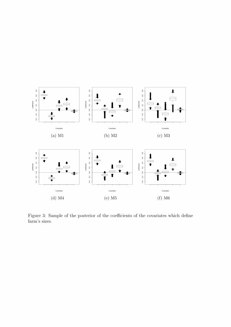
−0.

4−

0.2

0.0

0.2

0.4

0.6

0.8

Covariates

coef

ficie

nts

(a) M1

●●●●●●●●●●●●●●●●●●●●●●●●●●●●●●●●●●●●●●●●●●●●●●●●●●●●●●●●●●●●●●●●●●●●●●●●●●●●●●●●●●●●●●●●●●●●●●●●●●●●●●●●●●●●●●●●●●●●●●●●●●●●●●●●●●●●●●●●●●●●●●●●●●●●●●●●●●●●●●●●●●●●●●●●●●●●●●●●●●●●●●●●●●●●●●●●●●●●●●●●●●●●●●●●●●●●●●●●●●●●●●●●●●●●●●●●●●●●●●●●●●●●●●●●●●●●●●●●●●●●●●●●●●●●●●●●●●●●●●●●●●●●●●●●●●●●●●●●●●●●●●●●●●●●●●●●●●●●●●●●●●●●●●●●●●●●●●●●●●●●●●●●●●●●●●●●●●●●●●●●●●●●●●●●●●●●●●●●●●●●●●●●●●●●●●●●●●●●●●●●●●●●●●●●●●●●●●●

●●●●●

●●●●●●●●●●●●●●●●●●●●●●●●●●●●

●●●●●●●●●●●●●●●●●●

●●●●●●●●●●●●●●●●●●●●●●●●●●●●●●●●●●●●●●●●●●●●●●●●●●●●●●●●●●●●●●●●●●●●●●●●●●●●●●●●●●●●●●●●●●●●●●●●●●●●●●●●●●●●●●●●●●●●●●●●●●

●●●●●●●●●●●●●●●●●●●●●●●●●●●●●●●●●●●●●●●●●●●●●●●●●●●●●●●●●●●●●●●●●●●●●●●●●●●●●●●●●●●●●●●●●●●●●●●●●●●●●●●●●●●●●●●●●●●●●●●●●●●●●●●●●●●●●●●●●●●●●●●●●●●●●●●●●●●●●●●●●●●●●●●●●●●●●●●●●●●●●●●●●●●●●●●●●●●●●●●●●●●●●●●●●●●●●●●●●●●●●●●●●●●●●●●●●●●●●●●●●●●●●●●●●●●●●●●●●●●●●●●●●●●●●●●●●●●●●●●●●●●●●●●●●●●●●●●●●●●●●●●●●●●●●●●●●●●●●●●●●●●●●●●●●●●●●●●●●●●●●●●●●●●●●●●●●●●●●●●●●●●●●●●

●●●●●●●●●●●●●●●●●●●●●●●●●●●●●●●●●●●●●●●●●●●●●●●●●●●●●●●●●●●●●●●●●●●●●●●●●●●●●●●

●●●●●●●●●●●●●●●●●●●●●●●●●●●●●●●●●●●●●●●●●●

●●●●●●●●●●●●●●●●●●●

●●●●●●●●●●●●●●●●●●●●●●●●●●●●●●●●●●●●●●●●●●●●●●●●●●●●●●●●●●●●●●●●●●●●●●●●●●●●●●●●●●●●●●●●●●●●●●●●●●●●●●●●●●●●●●●●●●●●●●●●●●●●●●●●●●●●●●●●●●●●●●●●●●●●●●●●●●●●●●●●●●●●●●●●●●●●●●●●●●●●●●●●●●●●●●●●●●●●●●●●●●●●●●●●●●●●●●●●●●●●●●●●●●●●●●●●●●●●●●●●●●●●●●●●●●●●●●●●●●●●●●

●●●●●●●

●●●●●●●●●●●●●●●●●●●●●●●●●●●●●●●●●●●●●●●●●

●●●●●●

●●●●●●●●●●●

●●●●●●●●●●

●●●●●●●●●●●●●

●●●●●●●●●●●●●●●●●●●●●●●●●●●●●●●●●●●●●●●●●●●●●●●●●●●●

●●●●●●●●●●●●

●●●●●●●●●●●●●●●●●●●●●●●●●●●●●●

●●●●●●●●●●●●●●●●●●●●●●●●●●●●●●●●●●●●●●

●●●●●●

●●

●●●●●●●●●●●●●●●●

−0.

4−

0.2

0.0

0.2

0.4

0.6

0.8

Covariates

coef

ficie

nts

(b) M2

●●●●●●●●●●●●●●●●●●●●●●●●●●●●●●●●●●●●●●●●●●●●●●●●●●●●●●●●●●●●●●●●●●●●●●●●●●●●●●●●●●●●●●●●●●●●●●●●●●●●●●●●●●●●●●●●●●●●●●●●●●●●●●●●●●●●●●●●●●●●●●●●●●●●●●●●●●●●●●●●●●●●●●●●●●●●●●●●●●●●●●●●●●●●●●●●●●●●●●●●●●●●●●●●●●●●●●●●●●●●●●●●●●●●●●●●●●●●●●●●●●●●●●●●●●●●●●●●●●●●●●●●●●●●●●●●●●●●●●●●●●●●●●●●●●●●●●●●●●●●●●

●●●●●●●●●●●●●●●●●●●●●●●●●●●●●●●●●●●●●●●●●●●●●●●●●●●●●●●●●●●●●●●●●●●●●●●●●●●●●●●●●●●●●●●●●●●●●●●●●●●●●●●●●●●●●●●●●●●●●●●●●●●●●●●●●●●●●●●●

●●●●●●●●●●●●●●●●●●●●●●●●●●●●●●●●●●●●●●●●●●●●●●●●●●●●●●●●●●●●●●●●●●●●●●●●●●●●●●●●●●●●●●●●●●●●●●●●●●●●

●●●●●●●●●●●●●●●●●●●●●●●●●●●●●●●●●●●●●●●●●●●●●●●●●●●

●●●●●●●●●●●●●●●●●●●●●●●●●●●●●●●●●●●●●●●●●●●●

●●●●●●●●●●●●●

●●●●●●●●●●●●●●●●●●●●●●●●●●●●●●●●●●●●●●●●●●●●●●●●●●●●●●●●●●●●●●●●●●●●●●●●●●●●●●●●●●●●●●●●●●●●●●●●●●●●●●●●●●●●●●●●●●●●●●●●●●●●●●●●●●●●●●●●●●●●●●●●●●●●●●●●●●●●●●●●●●●●●●●●●●●●●●●●●●●●●●●●●●●●●●●●●●●●●●●●●●●●●●●●●●●●●●●●●●●●●●●●●●●●●●●●●●●●●●●●●●●●●●●●●●●●●●●●●●●●●●●●●●●●●●●●●●●●●●●●●●●●●●●●●●●●●●●●●●●●●●●●●●●●●●●●●●●●●●●●●●●●●●●●●●●●●●●●●●●●●●●●●●●●●●●●●●●●●●●●●●●●●●●●●●●●●●●●●●●●●●●●●●●●●●●●●●●●●●●●●●●●●●●●●●●●●●●●●●●●●●●●●●●●●●●●●●●●●●●●●●●●●●●●●●●●●●●●●●●●●●●●●●●●●●●●●●●

●●●●●●●●●●●●●●●●●●●●●●●●●●●●●●●●●●●●●●●●●●●●●●●●●●●●●●●●●●●●●●●●●●●●●●●●●●●●●●●●●

●●●●●●●●●●●●●●●●●●●●●●●●●●●●●●●●●●●●●●●●●●●●●●

●●●●●●●●●●●●●●●●●●●●●●

●●●●●●●●●●●●●●●●●●●●●●●

●●●●●●●●●●●●●●●●●●●●●●●●●●●●●●●●●●●●●●●●●●●●●●●●●●●●●●●●●●●●●●●●●●●●●●●●●●●●●●●●●●●●●●●●●●●●●

●●●●●●●●●●●●●●●●●●●●●●●●●●●●●●●●●●●●●●●●●●●●●●●●●●●●●●●●●●●●●●●●●●●●●●●●●●●●●●●●●●●●●●●●●●●●●●●●●●●●●●●●●●●●●●●●●●●●●●●●●●●●●●●●●●●●●●●●●●●●●●●●●●●●●●●●●●●●●●●●●●●●●●●●●●●●●●●●●●●●●●●●●●●●●●●●●●●●●●●●●●●●

●●●●●

●●●●●●●●●●●●●●●●●●●●●●●●●●●●●●●●●●●●●●●●●●●●●●●●●●●●●●●●●●●●●●●●●●●●●●●●●●●●●●●●●●●●●●●●●●●●●●●●●●●●●●●●●●●●●●●●●●●●●

●●●●●●●●●●●●●●●●●●●●●●●●●●●●●●●

●●

●●●●●●●●●●●●●●●●●●●●●●●●●●●●●●●●●●●●●●●●●●●●●●●●●●●●●●●●●●●●●●●●●●●●●●●●●●●●●●●●●●●●●●●●●●●●●●●●●●●●●●●●●●●●●●●●●●●●●●●●●●●●●●●●●●●●●●●●●●●●●●●●

●●●●●●●●●●●●●●

●●●●●●●●●●●●●●●●●●●●●●●●●●●●●●●●●●●●●●●●●●●●●●●●●●●●●●●●●●●●●●●

●●●●●●●●●●●●●●●●●●●●●●●●●●●●●●●●●●●●●●●●●●●●●●●●●●●●●●●●●●●●●●●●●●●●●●●●●●●●●●●●●●●●●●●●●●●●●●●●●●●●●●●●●●●●●●●●●●●●●●●●●●

●●●●●●●●●●●●●●●●●●●●●●●●●●●●●●●●●●●●●●●●●●●●●●●●●●●●●●●●●●●●●●●●●●●●●●●●●●●●●●●●●●●●●●●●●●●●●●●●●●●●●●●●●●●●●●●●●●●●●●●●●●●●●●●●●●●●●●●●●●●●●●●●●●●●●●●●●●●●●●●●●●●●●●●●●●●●●●●●●●●●●●●●●●●●●●●●●●●●●●●●●●●●●●●●●●●●●●●●●●●●●●●●●●●●●●

●●●●●●●●●●●●●●●●●●●●●●●●●●●●●●●●●●●●●●●●●●●●●●●●●●●●●●●●●●●●●●●●●●●●●●●●●●●●●●●●●●●●●●●●●●●●●●●●●●●●●●●●●●●●●●●●●●●●●●

●●●●●●●●●●●●●●●●●●●●●●●●●●●●●●●●●●●●●●●●●●●●●●●●●●●●●●●●●●●●●●●●●●●

●●●●●●●●●●●●●●●●●●●●●●●●●●●●●●●●●●●●●●●●●●●●●●●●●●●●●●●●●●●●●●●●●●●●●●●●●●●●●●●●●●

●●●●●●●●●●●●●●●●●●●●●●●●●●●●●●●●●●●●●●●●●●●●●●●●

●●●●●●●●●●●●●●●●●●●●●●●●●●●●●●●●●●●●●●●●●●●●●●●●●●●●●●●●●●●●●●●●●●●●●●●●●●●●●●●●●●●●●●●●●●●●●●●●●●●●●●●●●●●●●●●●●●●●●●●●●●●●

●●●●●●●●●●●●●●●●●●●●●●●●●●●●●●●●●●●●●●●●●●●●●●●●●●●●●●●●●●●●●●●●●●●●●●●●●●

●●●●●●●●●●●●●●●●●●●●●●●●●●●●●●●●●●●●●●●●●●●●●●●●●●●●●●●●●●●●●●●●●●●●●●●●●●●●●●●●●●●●●●●●●●●●●●●●●●●●●●●●●●●●●●●●●●●●●●●●●●●●●●●●●●●●●●●●●●●●●●●●●●●●●●●●●●●●●●●●●●●●●●●●●●●●●●●●●●●●●●●●●●●●●●●●●●●●●●●●●●●●●●●●●●●●●●●●●●●●●●●●●●●●●●●●●●●●●●●●●●●●●●●●●●●●●●●●●●●●●●●●●●●●●●●●●●●●●●●●●●●●●●●●●●●●●●●●●●●●●●●●●●●●●●●●●●●●●●●●●●●●●●●●●●●●●●●●●●●●●●●●●●●●●●●●●●●●●●●●●●●●●●●●●●●●●●●●●●●●●●●●●●●●●●●●●●●●●●●●●●●●●●●●●●●●●●●●●●●●●●●●●●●●●●●●●●●●●●●●●●●●●●●●●●●●●●●●●●●●●●●●●●●●●●●●●●●●●●●●●●●●●●●●●●●●●●●●●●●●●●●●●●●●●●●●●●●●●●●●●●●●●●●●●●●●●●●●●●●●●●

●●●●●●●●●●●

●

●●●●●●●●●●●●●●●●●●●●●●●●●●●●●●●●●●●●●●●●●●●●●●●●●●●●●●●●●●●●

●●●●●●●●●●●●●●●●●●●●●●●●●●●●●●●●●●●●●●●●●●●●●●●●●●●●●●●●●●●●●●●●●●●●●●●●●●●●●●●●●●●●●●●●●●●●●●●●●●●●●●●●●●●●●●●●●●●●●●●●●●●●●●●●●●●●●●

●●●●●●●●●●●●●●●●●●●●●●●●●●●●●●●●●●●●●●●●●●●●●●●●●●●●●●●●●●●●●●●●●●●●●●●●●●●●●●●●●●●●●●●●●●●●●●●●

−0.

4−

0.2

0.0

0.2

0.4

0.6

0.8

Covariates

coef

ficie

nts

(c) M3

●●●●●●●●●●●●●●●●●●●●●●●●●●●●●●●●●

●●●●●●●●●●●●●●●●●●●●●●●●●●●●●●●●●

●●●●●●●●●●●●

●●●●●●●●●●●●●●●●●●●●

●●●●●●●●●●●●●●●●●●●●●●●●●●●●●●●●●●●●●●●●●●●●●●●●●●●●●●●●●●●●

●●●●●●●●

●●●●●●●

●●

●●●●●●●●●●●●●●●●●●●●●●●●●●●●●●●

●●●●●●●●●●●●●●●●●●●●●●●●●●●●●●●●●●●●●●●●●●●●●●●●●●●●●●●●●●●●●●●●●●●●●●●●●●●●●●●●●●●●●●●●●●●●

●●●●●●●●●●●

●●●●●●●●●●●●●●●

●●●●●●●●●●●●●●●●●●●●●●●●●●●

●●●●●●●●

●

●●●●●●●●●●●●●●●●●●●●●●●●●●●●●●●●●●●●●●●●●●●●●●●●●●●●●●●●●●●●●●●●●●●●●●●●●●●●●●●●●●●●●●●●●●●●●●●●●●●●●●●●●●●●●●●●●●●●●●●●●●●●●●●●●●●●●●●●●●●●●●●●●●●●●●●●●●●●●●●●●●●●●●●●●●●●●●●●●●●●●●●●●●●●●●●●●●●●●●●●●●●●●●●●●●●●●●●●●●●●●●●●●●●●●●●●●●●●●●●●●●●●●●●●●●●●●●●●●●●●●●●●●●●●●●●●●●●●●●●●●●●

●●●●●●

●●●●●●

●●●●●●●●●●●●●●

●●●●●

●●●●●●●●●●●●●●●●●●●●●●●●●●●●●●●●●●●●●●●●●●●

●●

●●●

●●●●●●●●●●●●●●●●●●●●●●●●●●●●●●●●●●●●●●●●●●●●●●●●●●●●●●●●●●●●●●●●●

●●●●●●●●●●●●●●●●●●●●●●●●●●

●●●●●●●●●●●●●●●●●●●●●●●●●●●

●●●●●●●●●●●●●●●●●●●●●●●●●●●●●●●●●●●●●●●●●●●●●●●●●●●●●●●●●●●●●●●●●●●●●●●

●●●●●●●●●●●●●●●●●●●●●●●●●●●●●●●●●●●●●●●●●●●●●●●●●●●●●●●●●●●●●●●●●●●●●●●●●●●

●

●●●

●●●●

−0.

4−

0.2

0.0

0.2

0.4

0.6

0.8

Covariates

coef

ficie

nts

(d) M4

●●●●●●●●●●●●●●●●●●●●●●●●●●●●●●●●●●●●●●●●●●●●●●●●●●●●●●●●●●●●●●●●●●●●●●●●●●●●●●●●●●●●●●●●●●●●●●●●●●●●●●●●●●●●●●●●●●●●●●●●●●●●●●●●●●●●●●●●●●●●●●●●●●●●●●●●●●●●●

●●●●●●●●●●●●●●●●●●●●●●●●●●●●

●

●●●●

●

●●●●●●●●●●●●●●●●●●●●●●●●●●●●●

●●●●●●●●●●●●●●●●●●●●●●●●●●●●●●●●●●●●●●●●●●●●●●●●●●●●●●

●●●●●●●●●●●●●●●●●●●●●●●●●●●●●●●●●●●●●●●●●●●●●●●●●●●●●●●●●●●●●●●●●●●●●●●●●●●●●●●●●●●●●●●●●●●●●●●●●●●●●●●●●●●

●●

●●●●●●●●●●●●●●●●●●●●●●●●●●●●●●●●●●●●●●●●●●●●●●●●●●●●●●●●●●●●●●●

●●●●●●●

●●

●●●●●●●●●●●●●●●●●●●●●●●●●●●●●●●●●●●●●●●●●●●●●●●●●●●●●●●

●●●●●●●●●●●●●●●●●●●●●●●●●●●●●●●●●●●●●●●●●●●●●●●●●●●●●●●●●●●●●●●●●●●●●●●●●●●●●●●●●●●●●●●●●●●●●●●●●●●●●

●

●●●●●●●●●●●●●●●●●●●●●●●●●

●●●●●●●●●●●●●●●●●●●●●●●●●●●●●●●●●●●●●●●●●●●●●●●●●●●●●●●●●●●●●●●●●●●●●●●●●●●●●●●●●●●●●●●●●●●●●●●●●●●●●●●●●●●●●●●●●●●●●●●●●●●●●●●●●●●●●●●●●●●●●●●●●●●●●●●●●●●●●●●●●●●●●●●●●●●●●●●●●●●●●●●●●●●●●●●●●●●●●●●●●●●●●●●●●●●●●●●●●●●●●●●●●●●●●●●●●●●●●●●●●●●●●●●●●●●●●●●●●●●●●●●●●●●●●●●●●●●●●●●●●●●●●●●●●●●●●●●●●●●●●●●●●●●●●●●●●●●●

●●●●●●●●●●●●●●●

●●●●●●●●●●●●●●●●●●●●●●●●●●●●●●●●●●●●●●●●●●●●●●●●●●●●●●●●●●●●

●●●●●●●●●●●●●●●●●●●●●●●●●●●●●●●●●●●●●●●●●●●●●●●●●●●●●●●●●●●●●●●●●●●●●●●●●●●●●●●●●●●●●●

●●●●●●●●●●●●●●●●●●●●●●●●●●●●●●●●●●●●●●●●●●●●●●●●●●●●●●●●●●●●●●●●●●●●●●●●●●●●●●●●●

●●●●●●●●●●●●●●●●●●●●●●●●●●●●●●●●●●●●●●●●●●●●●●●●●●●●●●●●●●●●●●

●●●●●●●●●●

●●●●●●●●●●●●●●●●●●●●●●●●●●●●●●●●●●●●●●●●●●●●●●●●●●●●●●●●●●●●●●●●●●●●●●●●●●●●●●●●●●●●●●●●●●●●●●●●●●●●●●●●●●●●●●●●●●●●●●●●●●●●●●●●●●●●●●●●●●●●●●●●●●●●●●●●●●●●●●●●●●●●●●●●●●●●●●●●●●●●●●●●●●●●●●●●●●●●●●●●●●●●●●●●●●●●●●●●●●●●●●●●●●●●●●●●●●●●●●●●●●●

●●●●●●●●●●●●●●●●●●●●●●●●●●●●●●●●●●●●●●●●●●●●

●●●●●●●●●●●●●●●●●●●●●●●●●●●●●●●●●●●●●●●●●●●●●●●●●●●●●●●●●●●●●●●●●●●●●●●●●●●●●●●●●●●●●●●●●●●●●●●●●●●●●●●●●●●●●●●●●●●●●●●●●●●●●●●●●

●

●●●●●●●●●●●●●●●●●●●●●●●●●●●●●

●●●●●●●●●●●●●●●●●●●●●●●●●●●●●●●●●●●●●●●●●●●●●●●●●●●●●●●●●●●●●●●●●●●●●●●●●●●●●●●●●●●●●●●●●●●●●●●●●●●●●●●●●●●●●●●●●●●●●●●●●●●●●

●●●

●●●●●●●●●●●●●●●●●●●●●●●●●●●●●●●●●●●●●●●●●●●●●●●●●●●●●●●●●●●●●●●●

●●●●●●●●●●●

●●●●●●●●●●●●●●●●●●●●●●●●●●●●●●●●●●●●●●●

●

●●●●●●●●●●●●●●●●●●●●●●●●●●●●●●●●●●●●●●●●●●●●●●●●●●●●●●●●●●●●●●●●●●●●●●●●●●●●●●●●●●●●●●●●●●●●●●●●●●●●●●●●●●●●●●●●●●●●●●●●●●●●●●●●●●●●●

●●●●●●●●●●●●●●●●●●●●●●●●●●●●●●●●●●●●●●●●●

●●●●●●●●●●●●●●●●●●●●●●●●●●●●●●●●●●●●●●●●●●●●●●●●●●●●●●●●●●●●●

●●●●●●●●●●●●●●●●●●●

●●●●●●●●●●●●●●●●●●●●●●●●●●●●●●●●●●●●

●●

●●●●

●●●●●●●●●●●●●●●●●●

●●●●●●

●●

●●●●●●●●●●●●●●●●●●●●●

●●●●●●●●●●●●●●●●●●●●●●●●●●●●●●

●●

●●●

●●●●●●●●●●●●●●●●●●●●●●●●●●●●●●●●●●●●●●●●●●●●●●●●●●●●●●●●●●●●●●●●●●

●●●●●●●●●●●●●●●●●●●●●●●●●●●●●●●●●●●●●●●●●●●●●●●●●●●●●●●●●●●●●●●●●●●●●●●●●●●●●●●●●●●●●●●●●●●●●●●●●●●●●●●●●●●●

●●●●●●●●●●●●●●●●●●●●●●●●●●●●●●●●●●●●●●●●●●●●●●●●●●●●●●●●●●●●●●●●●●

●

●●●●●●

●●●●

●●●●●●●●●●●●●●●●●●●●●●●●●●●●●●●●●●●●●

●●●●●●●●●●●●●●●●●●●●●●●●●●●●●●●●●●●●●●●●●●●●●●●●●●●●●●●●●●●●●●●●●●●●●●●●●●●●●●●●●

●●●●●●●●●●

●●●●●

●●●●●●●●●●

●●●●●●●●●●●●●●●●●●●●

●●●

−0.

4−

0.2

0.0

0.2

0.4

0.6

0.8

Covariates

coef

ficie

nts

(e) M5

●●●●●●●●●●●●●●●●●●●●●●●●●●●●●●●●●●●●●●●●●●●●●●●●●●●●●●●●●●●●●●●●●●●●●●●●●●●●●●●●●●●●●●●●●●●●●●●●●●●●●●●●●●●●●●●●●●●●●●●●●●●●●●●●●●●●●●●●●●●●●●●●●●●●●●●●●●●●●●●●●●●●●●●●●●●●●●●●●●●●●●●●●●●●●●●●●●●●●●●●●●●●●●●●●●●●●●●●●●●●●●●●●●●●●●●●●●●●●●●●●●●●●●●●●●●●●●●●●●●●●●●●●●●●●●●●●●●●●●●●●●●●●●●●●●●●●●●●●●●●●●●●●●●●●●●●●●●●●●●●●●●●●●●●●●●●●●

●●●●●●●●●●●●●●●●●●●●●●●●●●●●●●●●●●●●●●●●●●●●●●●●●●●●●●●●

●●●●●●●●●●●●●●●

●●●●●●●●●●●●●●●●●●●●●●●●●●●●●●●●●●●●●●●●●●●●●●●●●●●●●●●●●●●●●●●●●●●●●●●●●●●●●●●●●●●●●●●●●●●●●●●●●●●●●●●●●●●●●●●●●●●●●●●●●●●●●●●●●●●●●●●●●●●●●●●●●●●●●●●●●●●●●●●●●●●●●●●●●●●●●●●●●●●●●●●●●●●●●●●●●●●●●●●●●●●●●●●●●●●●●●●●●●●●●●●●●●●●

●●●●●●●●●●●●●●●●●●●●●●●●●●●●●●●●●●●●●●●●●●●●●●●●●●●●●●●●●●●●●●●●●●●●●●●●●●●●●●●●●●●●●●●●●●●●●●

●●

●●●●●●●●●●●●●●●●●●●●●●●●●●●●●●●●●●●●●

●●●●●

●●●●●●●●●●●●●●●●●●●●

●●●●●●●●●●●●●●●●●●●●●●●●●●●●●●●●●●●●●●●●●●●●●●●●●●●●●●●●●●●●●●●●●●●●●●●●●●●●●●●●●●●●●●●●●●●●●●●●●●●●●●●●●●●●●●●●●●●●●●●●●●●●●●●●●●●●●●●●●●●●●●●●●●●●●●●●●●●●●●●●●●●●●●●●●●●●●●●●●●●●●●●●●●●●●●●●●●●●●●●●●●●●●●●●●●●●●●●●●●●●●●●●●●●●●●●●●●●●●●●●●●●●●●●●●●●●●●●●●●●●●●●●●●●●●●●●●●●●●●●●●●●●●●●●●●●●●●●●●●●●●●●●●●●●●●●●●●●●●●●●●●●●●●●●●●●●●●●●●●●●●●●●●●●●●●●●●●●●●●●●●●●●●●●●●●●●

●●●●●●●●●●●●●●●●●●●●●●●●●●●●●●●●●●●●●●●●●

●●●

●●●●●●●●●●●●●●●●●●●●

●●●●●●●●●●●●●●

●●●●●●●●●●●●●●●●●●●●●●●●●●●●●●●●●●●●●●●●●●●●●●●●●●●●●●●●●●●●●●●●●●●●●●●●●●●●●●●●●●●●●●●●●●●●●●●●●●●●●●●●●●●●●●●●●●●●●●●●●●●●●●●●

●●●●●●●●●●●●●●●●●●●●●●●●●●●●●●●●●●●●●●●●●●●●●●●●●●●●●●●●●●●●●●●●●●

●●●●●●●●●●●●●●●●●●●●●●●●●●●●●●●●●●●●●●●●●●●

●●●●●●●●●●●●●●●●●●●●●●●●●●●●●●●

●●●●●●●●●●●●●●●●●●●●●●●●●●●●●●●●●●●●●●●●●●●●●●●●●

●●●●●●●●●●●●●●●●●●●●●●●●●●●●●●●●●●●●●●

●●●●●●●●●●●●●●●●●●●●●

●●●●

●●●●●●●●●●●●●●●●●●●●●●●●●●●●●●

●

●●●●●●●●●●●●●●●●●●●●●●●●●●●●●●●●●

●●●●●●●●●●●●●●●●●●

●●●●●

●●●●●

●●●●●●●●●●●●●●●●●●●

●●●●●

●

●●●●●●●●●●●●●●●●●●●●

●●●●●●●●●●●●●●●●●●●●●●

●●●●●●●●●●●●●●●●●●●●●●●●●●●●●●●●●●●●●●●●●●●●●●●●●●●●●●●●

●●●●●●●●●●●●●●●●●●●●●●●●●●●●●●●●●

●●●●●●●●●●●●●●●●●●●●●●●●●●●●●●●●●●●●●●●●●●●●●●●●●●●●●●●●●●●●●●●●●●●●●●●●●●●●●●●●●●●●●●●●●●●●●●●●●●●

●

●●●●●●●●●●●●●●●●●●●●●●●●●●●●●●●●●●●●●●●●●●●●●●●●●●●●●●●●●●●●●●●●●●●●●●

●●●●●●●●●●●●●●●●●●●●●●●●●●●●●●●●●●●●●●●●●●●●●●●●●●●●●●●●●●●●●●●●●●●

●●●●●●●●●●●●●●●●●●●●●●●●●●●●●●●●●●●●●●●●●●●●●●●●●●●●●●●●●●●●●●●●●●●●●●●●●●●●●●●●●●●●●●●●●●●●●●●●●●●●●●●●●●●●●●●●●●●●●●●●●●●●●●●●●●●●●●●●●●●●●●●●●●●●●●●●●●●●●●●●●●●●●●●●●●●●●●●●●●●●●●●●●●●●●●●●●●●●●●●●●●●●●●●●●●●●●●●●●●●●●●●●●●●●●●●●●●●●●●●●●

●●●●●●●●●●●●

●●●

●●●●●●●●●●●●●●●●●●●●●●●●●●●●●

●●●●●●●●●●●●●●●●●●●●●●●●●●●●●●●●●●●●●●●●●●●●●●●●●●●●●●●●●●●●●●●●●●●●●●●●●●●●●●●●●●●●●●●●●●●●●●●●●●●●●●●●●●●●●●●●●●●●●●●●●●●●●●●●●

−0.

4−

0.2

0.0

0.2

0.4

0.6

0.8

Covariates

coef

ficie

nts

(f) M6

Figure 3: Sample of the posterior of the coefficients of the covariates which definefarm’s sizes.

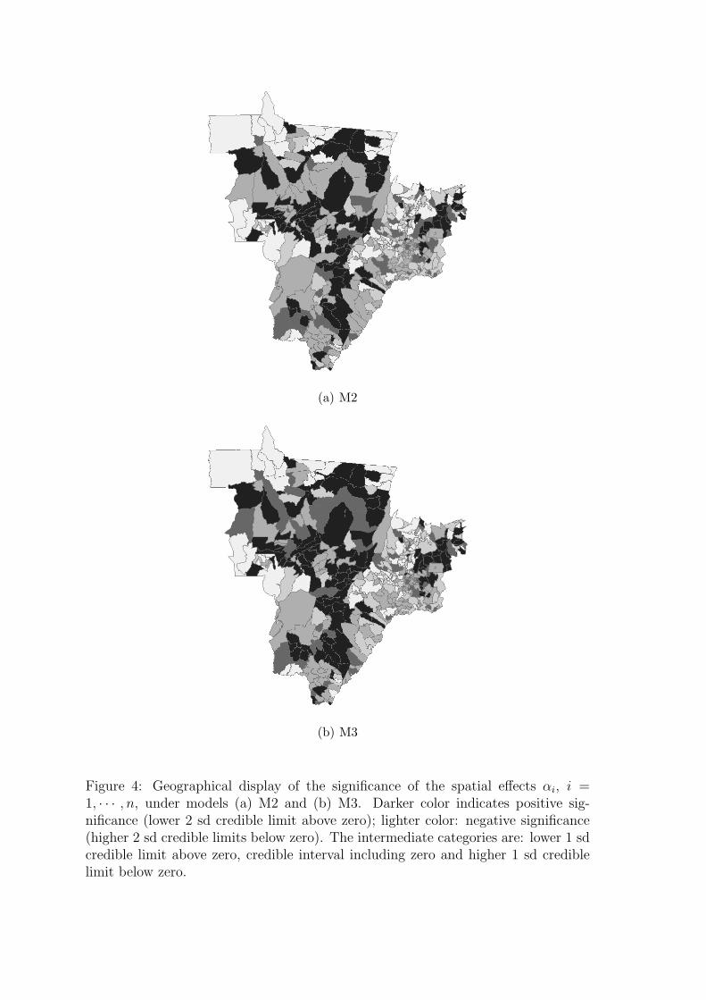
(a) M2

(b) M3

Figure 4: Geographical display of the significance of the spatial effects αi, i =1, · · · , n, under models (a) M2 and (b) M3. Darker color indicates positive sig-nificance (lower 2 sd credible limit above zero); lighter color: negative significance(higher 2 sd credible limits below zero). The intermediate categories are: lower 1 sdcredible limit above zero, credible interval including zero and higher 1 sd crediblelimit below zero.

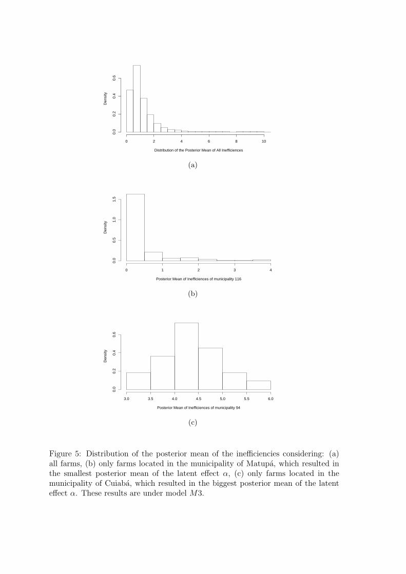
Distribution of the Posterior Mean of All Inefficiences

Den

sity

0 2 4 6 8 10

0.0

0.2

0.4

0.6

(a)

Posterior Mean of Inefficiences of municipality 116

Den

sity

0 1 2 3 4

0.0

0.5

1.0

1.5

(b)

Posterior Mean of Inefficiences of municipality 94

Den

sity

3.0 3.5 4.0 4.5 5.0 5.5 6.0

0.0

0.2

0.4

0.6

(c)

Figure 5: Distribution of the posterior mean of the inefficiencies considering: (a)all farms, (b) only farms located in the municipality of Matupa, which resulted inthe smallest posterior mean of the latent effect α, (c) only farms located in themunicipality of Cuiaba, which resulted in the biggest posterior mean of the latenteffect α. These results are under model M3.

Ipea – Institute for Applied Economic Research

PUBLISHING DEPARTMENT

CoordinationCláudio Passos de Oliveira

SupervisionEverson da Silva MouraReginaldo da Silva Domingos

TypesettingBernar José VieiraCristiano Ferreira de AraújoDaniella Silva NogueiraDanilo Leite de Macedo TavaresDiego André Souza SantosJeovah Herculano Szervinsk JuniorLeonardo Hideki Higa

Cover designLuís Cláudio Cardoso da Silva

Graphic designRenato Rodrigues Buenos

The manuscripts in languages other than Portuguese published herein have not been proofread.

Ipea Bookstore

SBS – Quadra 1 − Bloco J − Ed. BNDES, Térreo 70076-900 − Brasília – DFBrazilTel.: + 55 (61) 3315 5336E-mail: livraria@ipea.gov.br

Composed in Adobe Garamond 11/13.2 (text)Frutiger 47 (headings, graphs and tables)

Brasília – DF – Brazil

Ipea’s missionEnhance public policies that are essential to Brazilian development by producing and disseminating knowledge and by advising the state in its strategic decisions.