JSS Journal of Statistical SoftwareNovember 2017, Volume 81, Issue 6. doi: 10.18637/jss.v081.i06

Stochastic Frontier Analysis Using SFAMB for Ox

Jonathan HoltkampUniversity of Goettingen

Bernhard BrummerUniversity of Goettingen

Abstract

SFAMB is a flexible econometric tool designed for the estimation of stochastic frontiermodels. Ox is a matrix language used in different modules, with a console version freelyavailable to academic users. This article provides a brief introduction to the field ofstochastic frontier analysis, with examples of code (input and output) as well as a technicaldocumentation of member functions. SFAMB provides frontier models for both cross-sectional data and panel data (focusing on fixed effects models). Member functions canbe extended depending on the needs of the user.

Keywords: stochastic frontier analysis, panel data, Ox.

1. Introduction

SFAMB (stochastic frontier analysis using ‘Modelbase’) is a package for estimating stochasticfrontier production (as well as cost, distance, and profit) functions. It provides specificationsfor both cross-sectional data and panel data. SFAMB is written in Ox (Doornik 2009) and isoperated by writing small programs (scripts).

The console versions of Ox are free for research and educational purposes. Ox Console usesOxEdit to run programs, while the commercial version of the programming language, OxProfessional, uses the graphical user environment OxMetrics instead.

The structure of the paper is as follows. In the next section, we briefly introduce the econo-metric foundations and related literature. The first part focuses on the theory of models forcross-sectional and panel data. A subsection presents the specifications that are availablein SFAMB and mentions some related other software. Section 3 explains the usage of thepackage, which includes data structure, model formulation, and model output. Furthermore,it provides a detailed list of class member functions. For illustration, we present practicalexamples using real world data (Section 4) which are distributed with the package. We men-tion some possible extensions of SFAMB in Section 5. Finally, a technical appendix providesa brief overview of some underlying workings (Appendix A).

2 Stochastic Frontier Analysis Using SFAMB for Ox

2. Econometric methods of stochastic frontier analysis

2.1. Cross-sectional data

Basic approach – POOLED model

This section provides a brief introduction to stochastic frontier (SF) techniques. A more de-tailed introduction can be found in Coelli, Rao, O’Donnell, and Battese (2005) or Bogetoftand Otto (2010). More advanced material is covered in Kumbhakar and Lovell (2000). Thebasic problem in efficiency analysis lies in the estimation of an unobservable frontier (produc-tion, distance or cost) function from observable input and output data, together with pricedata when necessary. Standard estimation techniques like OLS are inappropriate in this set-ting as they aim to describe average relationships, which are not the focus of an efficiencymodel.

The basic approach was simultaneously developed by Aigner, Lovell, and Schmidt (1977)(ALS), and Meeusen and Van den Broeck (1977). The following example of a productionfrontier highlights its most important characteristics. The basic production frontier model isgiven by:

yi = α+ β>xi + vi − ui. (1)

On the left hand side, yi is the output (or some transformation of the output) of observationi (i = 1, 2, . . . , N). On the right hand side, xi is a K × 1 vector of inputs that producesoutput yi, and the vector β represents technology parameters to be estimated. The mostcommonly used transformation of the variables is the natural logarithm. The crucial part ofthis formulation is the composed error term given by εi = vi−ui, where vi represents statisticalnoise and ui represents inefficiency. Both error components are assumed to be independent ofeach other. Estimation is possible by means of maximum likelihood estimation (MLE) wheredistributional assumptions on the error components are required. The noise component is

a conventional two-sided error, distributed as viiid∼ N(0, σ2v). The inefficiency component is

a non-negative disturbance that can be modeled using several distributions.1 However, thetruncated normal and half-normal distributions are most frequently used and implemented inSFAMB (see Table 2). In case of the normal-truncated normal SF model, the random variable

ui is distributed as uiiid∼ N+(µ, σ2u). If µ is set to zero, the model becomes the normal-half

normal SF model.

Extensions of the basic SF approach allow us to model the location and scale of the ineffi-ciency distribution in a more flexible way. The corresponding covariates are often labeled asz-variables. Alvarez, Amsler, Orea, and Schmidt (2006) offer a comprehensive discussion ofthis topic and the so-called “scaling property”.

Another useful overview is given by Lai and Huang (2010) who summarize and categorizeseveral well-known models.2 The so-called KGMHLBC3 model parameterizes µ and originallyassumes the following inefficiency distribution, ui ∼ N+(µ0 + θ>zi, σ

2u). If µ is set to zero

1This text cannot provide a full overview of all relevant models. Kumbhakar and Lovell (2000) and morerecently Greene (2008) provide very detailed surveys on applied SF models.

2The following abbreviations used by Lai and Huang (2010) were already used by Alvarez et al. (2006).The abbreviation KGMHLBC was introduced by Wang and Schmidt (2002).

3Kumbhakar, Gosh, and McGuckin (1991); Huang and Liu (1994); Battese and Coelli (1995).

Journal of Statistical Software 3

and the scale is modeled using an exponential form, it becomes the RSCFG4 model, whereui ∼ N+(0, exp(2(δ0 + δ>zi))). The combination of both models leads to the following form,ui ∼ N+(µi = µ0 + θ>zi, σ

2u,i = exp(2(δ0 + δ>zi))), that according to Lai and Huang (2010)

could be labeled as a generalized linear mean (GLM) model.5

Jondrow, Lovell, Materov, and Schmidt (1982) present a point estimator of inefficiency, givenby E(ui|εi). Battese and Coelli (1988) show that if the dependent variable is in logarithms,a more appropriate estimator is the point estimator of technical efficiency, given by TE i =E(exp(−ui)|εi).

2.2. Panel data

Unobserved heterogeneity – LSDV model

Panel data provide additional information because each individual is observed over a certaintime period, where periods are indexed with t (t = 1, 2, . . . , T ). The respective productionfunction model, estimated by OLS, can be written as:

yit = αi + β>xit + vit. (2)

This formulation includes the time dimension, a conventional two-sided error vitiid∼ N(0, σ2v),

and an individual intercept αi. The model’s virtue originates from the identification of these Ntime-invariant parameters. These “fixed” effects absorb unmeasured time-invariant individualattributes, and hence, the model accounts for unobserved heterogeneity. One commonly usedname of this approach is “least squares with dummy variables” (LSDV).

Instead of estimating the dummy variables, the conventional strategy is to apply within-transformation to the dependent and independent variable(s), e.g., for an independent vari-able:

xit = xit − xi.

The observation on xit is transformed by subtracting the respective individual mean xi. Theresulting variable xit is a deviation from the mean. This procedure eliminates the individualeffects because αi = αi − αi = 0. The transformed variables are used for model estimation.After estimation, the individual effects are calculated as:

αi = yi − β>xi.

Schmidt and Sickles (1984) use the model in a frontier context. They interpret the individualwith the highest intercept as 100% technically efficient and determine the inefficiency of theremaining individuals as ui = max(α) − αi. Accordingly, efficiency scores are time-invariantand are given by TE i = E(exp(−ui)).

4Reifschneider and Stevenson (1991); Caudill, Ford, and Gropper (1995).5Actually, they label models that include the KGMHLBC form as generalized exponential mean (GEM)

models. The reason is that they refer to the exponential form of the model that has been proposed by Alvarezet al. (2006). Following the categorization of Lai and Huang (2010), the model implemented in SFAMB is aGLM model. Furthermore, note that in SFAMB the respective scale parameter in the POOLED model is (thenatural logarithm of) σu,i, and not σ2

u,i. While σ2u is often used, the original formulation of CFG involved σu.

4 Stochastic Frontier Analysis Using SFAMB for Ox

If (in)efficiency should be modeled as time-invariant or not, depends on the objective andempirical application (see Greene 2008 for a comprehensive discussion). Nevertheless, in alonger panel, the assumption of time-varying inefficiency will usually be attractive. This facthas motivated extensions of the above model as well as the development of other approaches.One famous example is the model of Battese and Coelli (1992) (BC92) that has been appliedin many empirical studies. This model specifies uit = exp(−η(t−T ))×ui, and nests the caseof persistent inefficiency (if η = 0). SFAMB does not support this model, but other packagesdo (see Table 3).

Unobserved heterogeneity in SFA: Dummy variables – TFE model

The approach of Schmidt and Sickles (1984) is a reinterpretation of the well-known paneldata model. However, there is no differentiation between heterogeneity and inefficiency. Acomplete panel SF model takes both components into account:

yit = αi + β>xit + vit − uit. (3)

This model is proposed by Greene (2005, p. 277) who labels it as the “true fixed effects[TFE] stochastic frontier model”. Estimation of this model requires the inclusion of all Ndummy variables, i.e., the number of intercepts to be estimated corresponds to the numberof individuals. With fixed T , the estimate of the error variance is inconsistent (incidentalparameters problem). Furthermore, it is likely to be biased as pointed out by Chen, Schmidt,and Wang (2014). This is a relevant issue since this estimate is required for the assessmentof inefficiency.

Elimination of dummies – WT model

Wang and Ho (2010) propose an extension to overcome the incidental parameters problem.Their model is based on deviations from means (within-transformation; WT):6

yit = β>xit + vit − uit. (4)

This represents either a normal-truncated normal or a normal-half normal SF model where

the noise component is distributed as vitiid∼ N(0, σ2v). Let the vector of transformed vit be

denoted by vi = (vi1, . . . , viT )>. This vector has a multivariate normal distribution, i.e.,vi ∼ MN (0,Π), where Π is a T × T covariance matrix.7

The specification of time-varying inefficiency (uit) is more involved. Here, the (“basic”) ineffi-

ciency component is assumed to be producer-specific, but time-invariant, i.e., u∗iiid∼ N+(µ, σ2u),

where µ is equal to zero in the case of a half-normal distribution. Inefficiency varies over timeby means of a scaling function:

uit = u∗i × hit = u∗i × f(δ>zit) = u∗i × exp(δ>zit),

where zit is a vector of time-varying, producer-specific covariates. The transformed ineffi-ciency component results from the transformation of the scaling function:

uit = u∗i × hit.6They also demonstrate how the model can be estimated by first-differencing.7The panel may be unbalanced.

Journal of Statistical Software 5

Wang and Ho (2010) present the conditional expectation of uit in their Equation 30; efficiencyestimates are given by TE it = E(exp(−uit|εit)). The individual effects are calculated as:

αi = yi − β>xi + ui.

Consistent estimation with time-varying inefficiency – CFE model

Consistent estimation of the fixed effects SF model given in Equation 3 is demonstrated byChen et al. (2014). Their approach is also based on deviations from means (Equation 4), butthe CFE (consistent fixed effects) model allows inefficiency to vary over individuals and time,without an auxiliary function.

The approach is characterized by two features, within-transformation and the T−1 deviations,as well as by the use of a more general distributional theory. Firstly, within-transformationremoves the incidental parameters. Secondly, the model’s likelihood function is derived fromthe first T − 1 deviations, i.e., from the vector ε∗i = (εi1, . . . , εi,T−1)

>. This strategy achievesan implicit correction of the error variance.8 The approach is based on the closed skew normal(CSN) distribution.9

The composed error, ε = v − u, has a skewed distribution (to the left) due to the non-negativeness of u. Accordingly, the standard (half-normal) SF model has a skew normaldistribution, with skewness parameter λ and density:

f(ε) =2

σφ( εσ

)Φ(−λ ε

σ

).

While the skew normal distribution is a generalization of the normal distribution, it can begeneralized itself by using the CSN distribution. The composed error has a CSN distribution,which is expressed by:

εit ∼ CSN 1,1(0, σ2,−λ

σ, 0, 1).

The density of a CSN p,q-distribution includes a p-dimensional pdf and a q-dimensional cdf of anormal distribution. The five associated parameters describe location, scale, and skewness, aswell as the mean vector and covariance matrix in the cdf. With panel data, the T -dimensionalvector εi = (εi1, . . . , εiT )> is distributed as:

εi ∼ CSN T,T (0T , σ2IT ,−

λ

σIT , 0T , IT ),

where I is the identity matrix. Chen et al. (2014, p. 67) make use of the fact that the CSNdistribution is “closed under linear combination”, and partition the vector εi into its mean εiand its first T−1 deviations ε∗i . The model’s likelihood function is derived from ε∗i . Therefore,it is free of incidental parameters, and the parameters to be estimated are β, λ, and σ2 – as

8With regards to the degrees of freedom, the correction accounts for the N individuals: df = NT−N−K =N(T − 1) −K.

9Chen et al. (2014) explain how the SF model is related to the CSN distribution and present the requiredproperties of CSN distributed random variables. Another plain introduction to the CSN distribution in theSF context is provided by Brorsen and Kim (2013).

6 Stochastic Frontier Analysis Using SFAMB for Ox

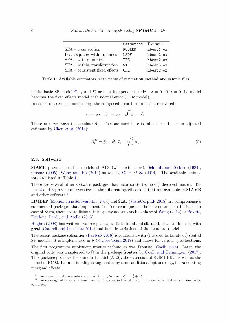
SetMethod Example

SFA – cross section POOLED hbest1.ox

Least squares with dummies LSDV hbest2.ox

SFA – with dummies TFE hbest2.ox

SFA – within-transformation WT hbest3.ox

SFA – consistent fixed effects CFE hbest2.ox

Table 1: Available estimators, with name of estimation method and sample files.

in the basic SF model.10 εi and ε∗i are not independent, unless λ = 0. If λ = 0 the modelbecomes the fixed effects model with normal error (LSDV model).

In order to assess the inefficiency, the composed error term must be recovered:

εit = yit − yit = yit − β>xit − αi.

There are two ways to calculate αi. The one used here is labeled as the mean-adjustedestimate by Chen et al. (2014):

αMi = yi − β>xi +

√2

πσu. (5)

2.3. Software

SFAMB provides frontier models of ALS (with extensions), Schmidt and Sickles (1984),Greene (2005), Wang and Ho (2010) as well as Chen et al. (2014). The available estima-tors are listed in Table 1.

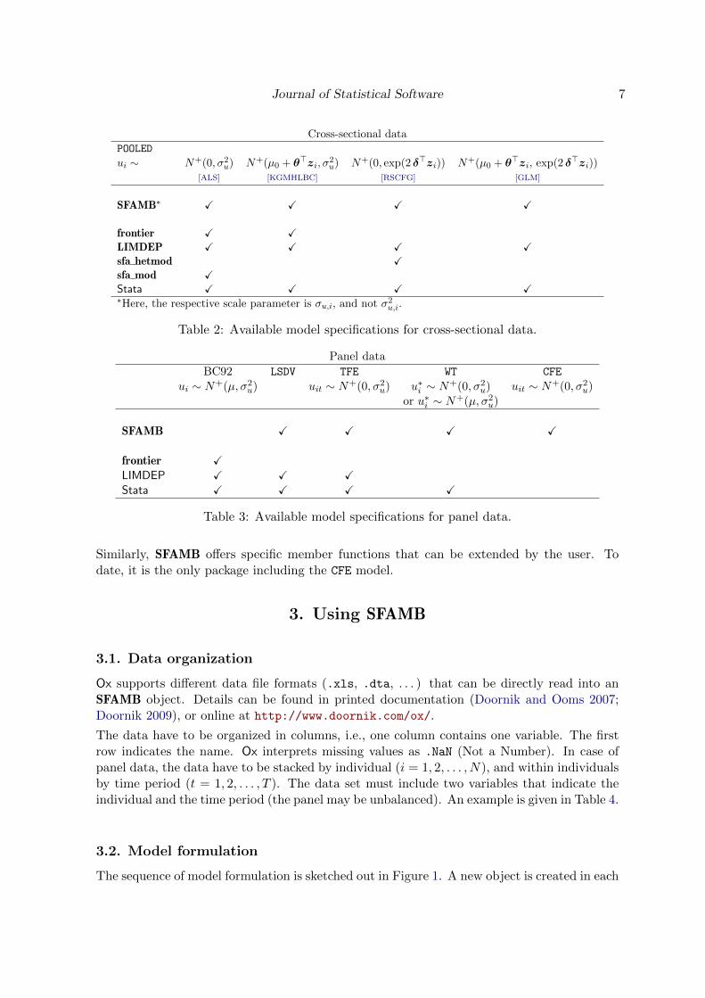
There are several other software packages that incorporate (some of) these estimators. Ta-bles 2 and 3 provide an overview of the different specifications that are available in SFAMBand other software.11

LIMDEP (Econometric Software Inc. 2014) and Stata (StataCorp LP 2015) are comprehensivecommercial packages that implement frontier techniques in their standard distributions. Incase of Stata, there are additional third-party add-ons such as those of Wang (2012) or Belotti,Daidone, Ilardi, and Atella (2013).

Hughes (2008) has written two free packages, sfa hetmod and sfa mod, that can be used withgretl (Cottrell and Lucchetti 2014) and include variations of the standard model.

The recent package spfrontier (Pavlyuk 2016) is concerned with (the specific family of) spatialSF models. It is implemented in R (R Core Team 2017) and allows for various specifications.

The first program to implement frontier techniques was Frontier (Coelli 1996). Later, theoriginal code was transferred to R in the package frontier by Coelli and Henningsen (2017).This package provides the standard model (ALS), the extension of KGMHLBC as well as themodel of BC92. Its functionality is augmented by some additional options (e.g., for calculatingmarginal effects).

10The conventional parameterization is: λ = σu/σv and σ2 = σ2u + σ2

v.11The coverage of other software may be larger as indicated here. This overview makes no claim to be

complete.

Journal of Statistical Software 7

Cross-sectional data

POOLED

ui ∼ N+(0, σ2u) N+(µ0 + θ>zi, σ2u) N+(0, exp(2 δ>zi)) N+(µ0 + θ>zi, exp(2 δ>zi))

[ALS] [KGMHLBC] [RSCFG] [GLM]

SFAMB∗ X X X X

frontier X XLIMDEP X X X Xsfa hetmod Xsfa mod XStata X X X X∗Here, the respective scale parameter is σu,i, and not σ2u,i.

Table 2: Available model specifications for cross-sectional data.

Panel data

BC92 LSDV TFE WT CFE

ui ∼ N+(µ, σ2u) uit ∼ N+(0, σ2u) u∗i ∼ N+(0, σ2u) uit ∼ N+(0, σ2u)or u∗i ∼ N+(µ, σ2u)

SFAMB X X X X

frontier XLIMDEP X X XStata X X X X

Table 3: Available model specifications for panel data.

Similarly, SFAMB offers specific member functions that can be extended by the user. Todate, it is the only package including the CFE model.

3. Using SFAMB

3.1. Data organization

Ox supports different data file formats (.xls, .dta, . . . ) that can be directly read into anSFAMB object. Details can be found in printed documentation (Doornik and Ooms 2007;Doornik 2009), or online at http://www.doornik.com/ox/.

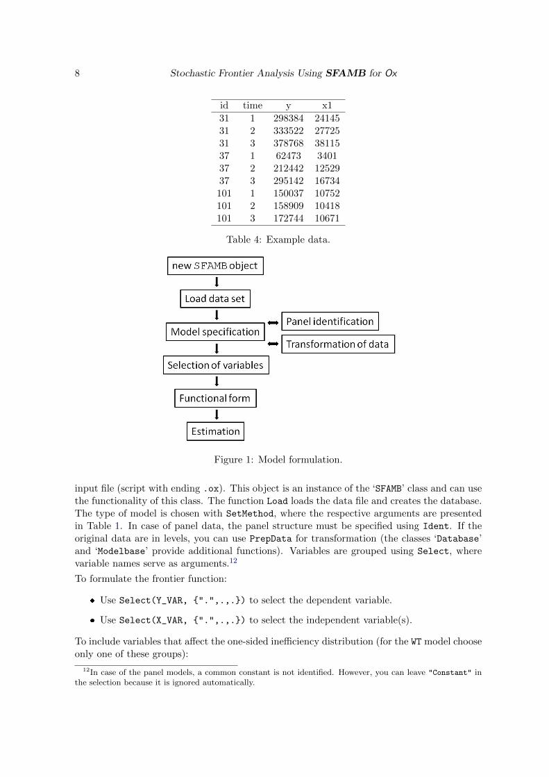
The data have to be organized in columns, i.e., one column contains one variable. The firstrow indicates the name. Ox interprets missing values as .NaN (Not a Number). In case ofpanel data, the data have to be stacked by individual (i = 1, 2, . . . , N), and within individualsby time period (t = 1, 2, . . . , T ). The data set must include two variables that indicate theindividual and the time period (the panel may be unbalanced). An example is given in Table 4.

3.2. Model formulation

The sequence of model formulation is sketched out in Figure 1. A new object is created in each

8 Stochastic Frontier Analysis Using SFAMB for Ox

id time y x1

31 1 298384 2414531 2 333522 2772531 3 378768 3811537 1 62473 340137 2 212442 1252937 3 295142 16734101 1 150037 10752101 2 158909 10418101 3 172744 10671

Table 4: Example data.

Figure 1: Model formulation.

input file (script with ending .ox). This object is an instance of the ‘SFAMB’ class and can usethe functionality of this class. The function Load loads the data file and creates the database.The type of model is chosen with SetMethod, where the respective arguments are presentedin Table 1. In case of panel data, the panel structure must be specified using Ident. If theoriginal data are in levels, you can use PrepData for transformation (the classes ‘Database’and ‘Modelbase’ provide additional functions). Variables are grouped using Select, wherevariable names serve as arguments.12

To formulate the frontier function:

� Use Select(Y_VAR, {".",.,.}) to select the dependent variable.

� Use Select(X_VAR, {".",.,.}) to select the independent variable(s).

To include variables that affect the one-sided inefficiency distribution (for the WT model chooseonly one of these groups):

12In case of the panel models, a common constant is not identified. However, you can leave "Constant" inthe selection because it is ignored automatically.

Journal of Statistical Software 9

� Use Select(U_VAR, {".",.,.}) to select variables that shift the individual locationparameter of the distribution, µi.

� Use Select(Z_VAR, {".",.,.}) to select variables that affect the scale parameter ofthe distribution, σu,i or σ2u,i.

SetTranslog can be used to choose the functional form of the frontier function. In caseof the translog specification, we recommend to normalize the variables by the respectivesample means. Estimation of the model is executed via Estimate. For more details, see thedocumentation of member functions in Section 3.4.

3.3. Model output

Besides standard results, some model-specific numbers are printed after estimation.

Cross-sectional data

Specific numbers for model POOLED:

gamma was defined by Battese and Corra (1977) and is given by γ = σ2u/σ2 = σ2u/(σ

2v + σ2u),

where σ2u = 1n

∑i exp(2 δ>zi).

VAR(u)/VAR(total) describes the variance decomposition of the composed error term. Theshare of the variance of u in the total variance of the composed error is given byVAR[u]/VAR[ε] = [(π − 2)/π]σ2u/[(π − 2)/π]σ2u + σ2v , see Greene (2008, p. 118), whereσ2u = 1

n

∑i exp(2 δ>zi).

Test of one-sided err provides a likelihood ratio test statistic for the presence of ineffi-ciency, i.e., for the null hypothesis H0: γ = 0. The critical value cannot be taken froma conventional χ2-table, see Kodde and Palm (1986).

Panel data

Specific numbers for model LSDV:

sigma_e describes σv, the square root of the corrected error variance, σ2v = SSRN(T−1)−K . This

estimate is also used to compute the standard errors.

AIC1 (all obs) is given by AIC1 = −2 lnL + 2 (K + 1); it uses the likelihood function

lnL = −NT2 ln(2π)− NT

2 ln(σ2)−∑

i

∑t v

2it

2σ2 with the uncorrected σ2 = SSRNT .

AIC2 uses a different formula for the criterion, AIC2 = ln(SSRNT ) + (2 K+NNT ); that does not

require the likelihood function and considers the number of individuals in the penaltyterm.

Specific number for models TFE, WT and CFE:

lambda given by λ = σu/σv .

10 Stochastic Frontier Analysis Using SFAMB for Ox

3.4. Class member functions

These functions (user interface) together with the data members build up the ‘SFAMB’ class.Some internal functions are not listed here. The interested user may consult the package’sheader file and source code file. Note that the class derives from the Ox ‘Modelbase’ class,and hence, all underlying functions may be used.13

AiHat AiHat();

Return valueReturns the calculated individual effects αi, N × 1 vector.Description– Only panel data – These values can be obtained after estimation, see Section 2 for therespective formulas.

Different functions to extract data:Return valueDifferent vectors or matrices.DescriptionThese functions can be used with convenient (‘Database’) functions such as Save, Renewor savemat.

IDandPer(); is an NT×2 matrix with the ID of the individual (e.g., 1, 1, 1, 2, . . . , N,N)in the first column and the individual panel length Ti in the second column. – Onlypanel data –

GetLLFi(); returns the individual log-likelihood values. It is an NT ×1 vector for bothPOOLED model and LSDV model, but an N × 1 vector for the other models.

GetResiduals(); returns the (composed) residual of the respective observation, NT×1vector.

GetTldata(); returns the corresponding vectors of Y , X, square, and cross terms ofX. – Use with SetTranslog() –

GetMeans(); returns the means of Y - and X-variables, N × (K + 1) matrix. – Onlypanel data –

GetWithins(); returns the within-transformed Y - and X-variables, NT × (K + 1)matrix. – Only panel data –

DropGroupIf DropGroupIf(const mifr);

No return valuesDescription– Only panel data – Allows the exclusion of a whole individual from the sample if thecondition in one (single) period is met. Call after function Ident.

mifr is the condition that specifies the observation to be dropped, see the documenta-tion of selectifr.

Elast Elast(const sXname);

Return value13The ‘Modelbase’ class derives from the ‘Database’ class. Accordingly, the member functions of ‘Database’

are available in SFAMB.

Journal of Statistical Software 11

Returns the calculated output elasticities and the respective t-values for the specified(single) input variable (for all sample observations).Description– Use with SetTranslog() – Only if a translog functional form is used, NT × 2 matrix.The elasticity is calculated for each observation of the sample: the output elasticity ofinput k is given by ∂ ln yi/∂ ln xki . The t-values are calculated using the delta method(Greene 2012), extracting the required values from the data and covariance matrix ofthe parameter estimates.

sXname is the name of the corresponding input variable (string).

GetResults GetResults(const ampar, const ameff, const avfct, const amv);

No return valuesDescription– Only POOLED model – This function can be used to store the results of the estimationprocedure for further use. All four arguments should be addresses of variables.

mpar consists of a Npar × 3 matrix, where Npar is the number of parameters in themodel. The first column contains the coefficient estimates, the second column thestandard errors, and the third column the appropriate probabilities.

eff consists of a Nobs×3 matrix, where Nobs is the number of total observations. Thefirst column holds the point estimate for technical efficiency, the second and thirdcolumns contain the upper and lower bound of the (1− α) confidence interval.

fct holds some likelihood function values (OLS and ML), as well as some informationon the correct variance decomposition of the composed error term.

v variance-covariance-matrix.

Ident Ident(const vID, const vPer);

No return valuesDescription– Only panel data – Identifies the structure of the panel.

vID is an NT × 1 vector holding the identifier (integer) of the individual.

vPer is an NT × 1 vector holding the identifier (integer) of the time period.

Ineff Ineff();

Return valueReturns point estimates of technical inefficiency, NT × 1 vector.DescriptionThese predictions are given by the conditional expectation of u, see Section 2 for details.

PrepData PrepData(const mSel, iNorm);

Return valueReturns logarithms of the specified variables, either normalized or not.DescriptionThis function expects your data in levels and can do two things: It takes logarithms ofyour specified variables (if iNorm = 0) or it normalizes your data (by the sample meanif iNorm = 1), before taking logarithms. The transformed variable should receive a newname.

12 Stochastic Frontier Analysis Using SFAMB for Ox

mSel is a NT × k matrix holding the respective Y - and X-variables.

iNorm is an integer: 0=no normalization; 1=normalization;

SetConfidenceLevel SetConfidenceLevel(const alpha);

No return valuesDescription– Only POOLED model – This function expects a double constant, indicating the errorprobability for the construction of confidence bounds (default 0.05).

SetPrintDetails SetPrintDetails(const bool);

No return valuesDescription– Not for LSDV model – Prints starting values, warnings and elapsed time if bool 6= 0.

SetRobustStdErr SetRobustStdErr(const bool);

No return valuesDescription– Only POOLED model – By default, robust standard errors are used for the cross-sectionalmodel. Use FALSE to switch off this setting.

SetStart SetStart(const vStart);

No return valuesDescriptionThis function expects a column vector of appropriate size (K + 2), containing startingvalues for the maximum likelihood iteration. If the function is not called at all, OLSvalues are used in conjunction with a grid search for the SFA-specific parameter(s)σ2 = σ2v + σ2u. If only (K) technology parameters are given, the grid search is alsoapplied.

SetTranslog SetTranslog(const iTl);

No return valuesDescriptionThis function expects an integer to control the construction of additional regressorsfrom the selected X-variables.

� A value of zero indicates no further terms to be added, e.g., for a log-linear model,this corresponds to the Cobb-Douglas form.

� A value of one indicates that all square and cross terms of all independent variablesshould be constructed, e.g., for a log-linear model, this corresponds to the fulltranslog form.

� An integer value of k > 1 indicates that the square and cross terms should beconstructed for only the first k independent variables (useful when the regressormatrix contains dummy variables).

TE TE();

Return valueReturns point estimates of technical efficiency, NT × 1 vector.Description

Journal of Statistical Software 13

These predictions are given by the conditional expectation of exp(−u), see Section 2 fordetails.

TEint TEint(const dAlpha);

Return valueReturns point estimates of technical efficiency as well as lower and upper bounds.Description– Only POOLED model – This function expects a double constant, indicating the errorprobability for the construction of confidence bounds (default 0.05); for details seeHorrace and Schmidt (1996), for an application Brummer (2001). It returns an NT × 3matrix structured as (point estimate – lower bound – upper bound).

TestGraphicAnalysis TestGraphicAnalysis();

No return valuesDescriptionOnly useful in conjunction with the free Ox package GnuDraw (Bos 2014), which is an Ox

interface to gnuplot (gnuplot Team 2015). This function draws two (or three) graphs:A histogram of the efficiency point estimates and a respective boxplot. It displaysan additional graph in case of the POOLED model, depicting the interval estimates oftechnical efficiency at the specified significance.

4. Examples

4.1. Example: hbest1.ox

The first example is a generalized linear mean (GLM) model, where ui ∼ N+(µ, σu,i =exp(δ0 + δ>zi)). The original data are in levels and are transformed using member functionPrepData to accommodate the translog functional form. The data are a subset of FAO/USDAdata prepared by Fuglie (2012), including Sub-Saharan African countries and South Africa.

General usage and details of the Ox language are explained in Doornik and Ooms (2007). Thesample file hbest1.ox is presented below. At the beginning of each program some headerfiles are linked in:

#include <oxstd.h>

#include <packages/gnudraw/gnudraw.h>

#import <packages/sfamb/sfamb>

The first file, the so-called standard header, ensures that all standard library functions canbe used. The second line includes the header file of GnuDraw (Bos 2014), an Ox interface tognuplot (gnuplot Team 2015). If it is not installed or you do not want to use this package,delete this line. However, graphics output will then be disabled in the free Ox Console version(in the commercial OxMetrics version, graphics would still be available). Alternatively, youcan comment it out via //:

// #include <packages/gnudraw/gnudraw.h>

14 Stochastic Frontier Analysis Using SFAMB for Ox

The third line imports the (compiled) source code of the package (you may also use #include

<packages/sfamb/sfamb.ox>). Each Ox program is executed by the main() function thatcontains the main loop of Ox.

main(){

...

}

The next steps outlined follow the structure of Figure 1. A new object of class ‘Sfa’ has tobe declared.

decl fob = new Sfa();

The data are loaded with a call to the member function Load. The argument of SetMethodchooses the respective estimator (see Table 1). Here, the model for cross-sectional data isspecified. The function SetConstant creates a constant (intercept).

fob.Load("USDAafrica.xls");

fob.SetMethod(POOLED);

fob.SetConstant();

Data are either used directly or prepared within the code. Here, the output variable, fiveinput variables, and a time variable are transformed where logarithms of the mean-normalizedinputs (output) are used.14 New names are assigned to the prepared variables. These namesare used for further instructions. The function Info is useful here because it prints summarystatistics, thereby allowing the transformed data to be checked. The program always stopsat an exit function (that is why it is commented out here).

decl inorm = 1;

fob.Renew(fob.PrepData(fob.GetVar("output"), inorm), "lny");

fob.Renew(fob.PrepData(fob.GetVar("labour"), inorm), "lnlab");

fob.Renew(fob.PrepData(fob.GetVar("land"), inorm), "lnland");

fob.Renew(fob.PrepData(fob.GetVar("machinery"), inorm), "lnmac");

fob.Renew(fob.PrepData(fob.GetVar("fertilizer"), inorm), "lnfert");

fob.Renew(fob.GetVar("time") - meanc(fob.GetVar("time")), "trend");

// fob.Info(); exit(1);

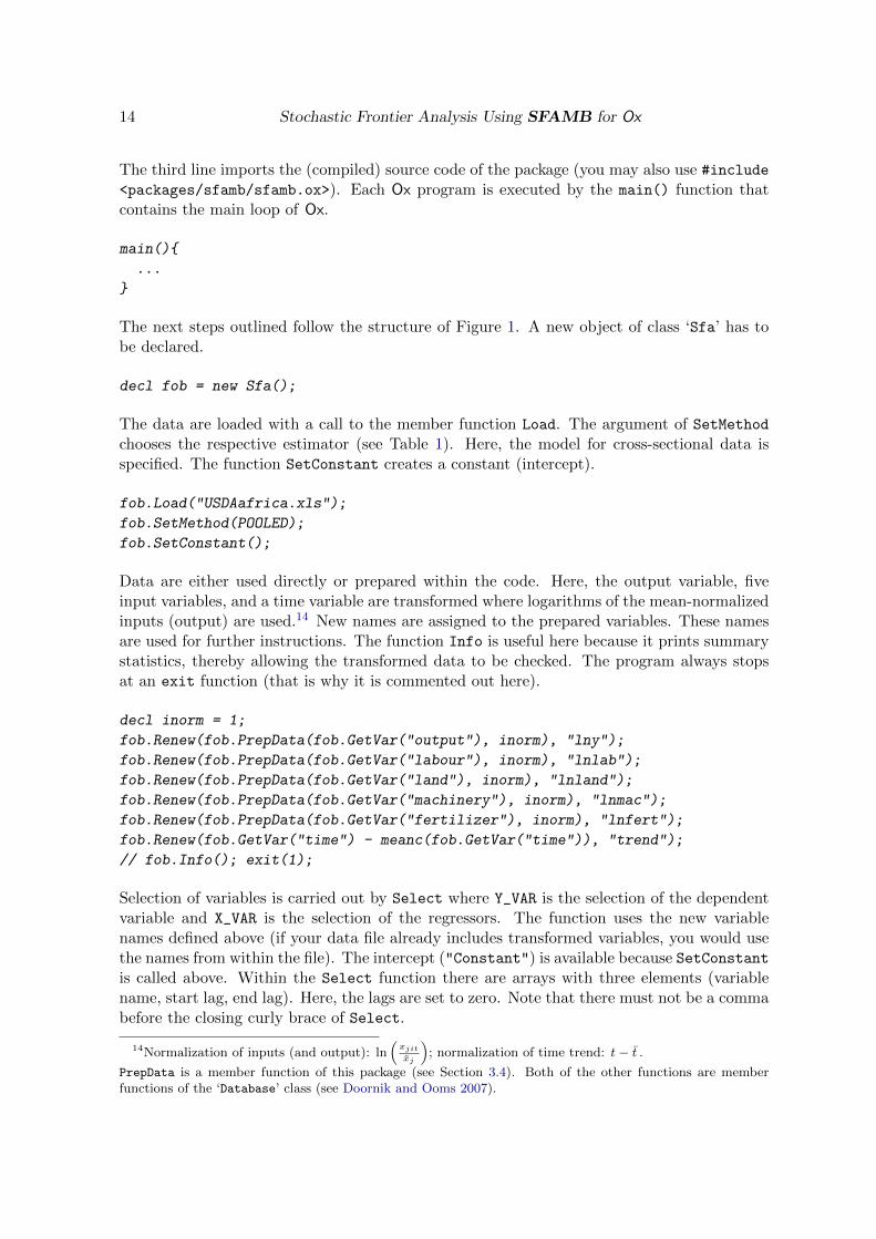
Selection of variables is carried out by Select where Y_VAR is the selection of the dependentvariable and X_VAR is the selection of the regressors. The function uses the new variablenames defined above (if your data file already includes transformed variables, you would usethe names from within the file). The intercept ("Constant") is available because SetConstantis called above. Within the Select function there are arrays with three elements (variablename, start lag, end lag). Here, the lags are set to zero. Note that there must not be a commabefore the closing curly brace of Select.

14Normalization of inputs (and output): ln(

xjit

xj

); normalization of time trend: t− t .

PrepData is a member function of this package (see Section 3.4). Both of the other functions are memberfunctions of the ‘Database’ class (see Doornik and Ooms 2007).

Journal of Statistical Software 15

fob.Select(Y_VAR, {"lny", 0, 0});

fob.Select(X_VAR, {

"Constant", 0, 0,

"lnlab", 0, 0,

"lnland", 0, 0,

"lnmac", 0, 0,

"lnfert", 0, 0,

"trend", 0, 0

});

The above selections define the production frontier. Additional covariates associated withthe underlying inefficiency distribution can be introduced (POOLED and WT model). Covariatesused to model the location parameter of the distribution are selected in the group U_VAR.Here, only "Constant" is selected, meaning that µ 6= 0, but additional variables could beincluded.

fob.Select(U_VAR, {

"Constant", 0, 0

});

Likewise, covariates used to model the scale of the distribution are selected in the groupZ_VAR, i.e., these variables parameterize σu,i (in case of the WT model, it is σ2u,i).

fob.Select(Z_VAR, {

"Constant", 0, 0,

"lnlab", 0, 0,

"lnland", 0, 0,

"lnmac", 0, 0,

"lnfert", 0, 0

});

The next three lines allow for different adjustments. SetSelSample is required and can beused to choose a subset of the data (here: full sample). SetPrintSfa ensures that estimationoutput is printed. MaxControl is an optional function that allows for documentation andadjustments of the maximization procedure.

fob.SetSelSample(-1, 1, -1, 1);

fob.SetPrintSfa(TRUE);

MaxControl(1000, 10, TRUE);

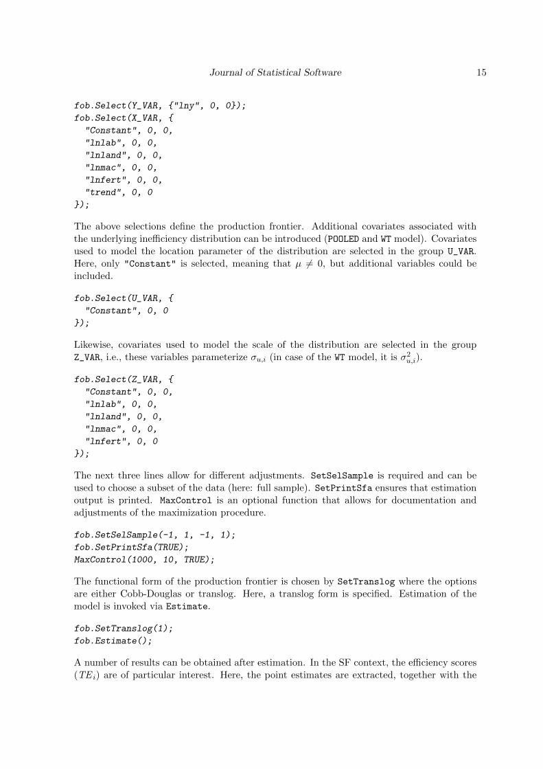
The functional form of the production frontier is chosen by SetTranslog where the optionsare either Cobb-Douglas or translog. Here, a translog form is specified. Estimation of themodel is invoked via Estimate.

fob.SetTranslog(1);

fob.Estimate();

A number of results can be obtained after estimation. In the SF context, the efficiency scores(TE i) are of particular interest. Here, the point estimates are extracted, together with the

16 Stochastic Frontier Analysis Using SFAMB for Ox

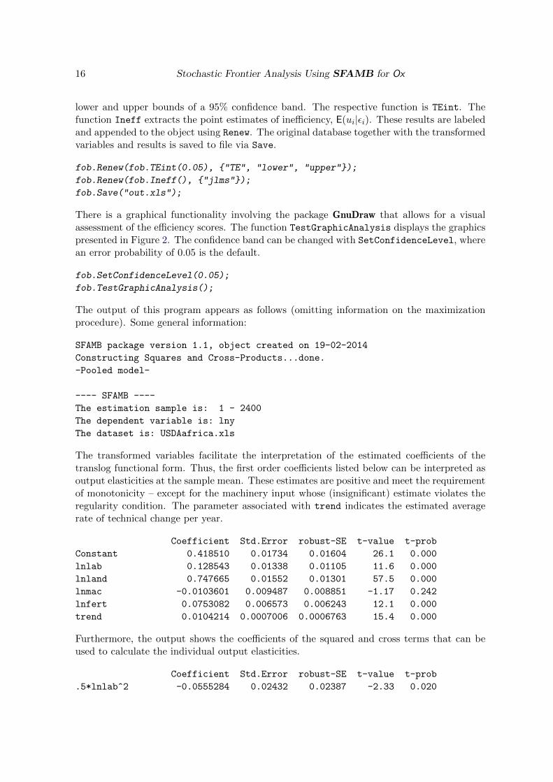
lower and upper bounds of a 95% confidence band. The respective function is TEint. Thefunction Ineff extracts the point estimates of inefficiency, E(ui|εi). These results are labeledand appended to the object using Renew. The original database together with the transformedvariables and results is saved to file via Save.

fob.Renew(fob.TEint(0.05), {"TE", "lower", "upper"});

fob.Renew(fob.Ineff(), {"jlms"});

fob.Save("out.xls");

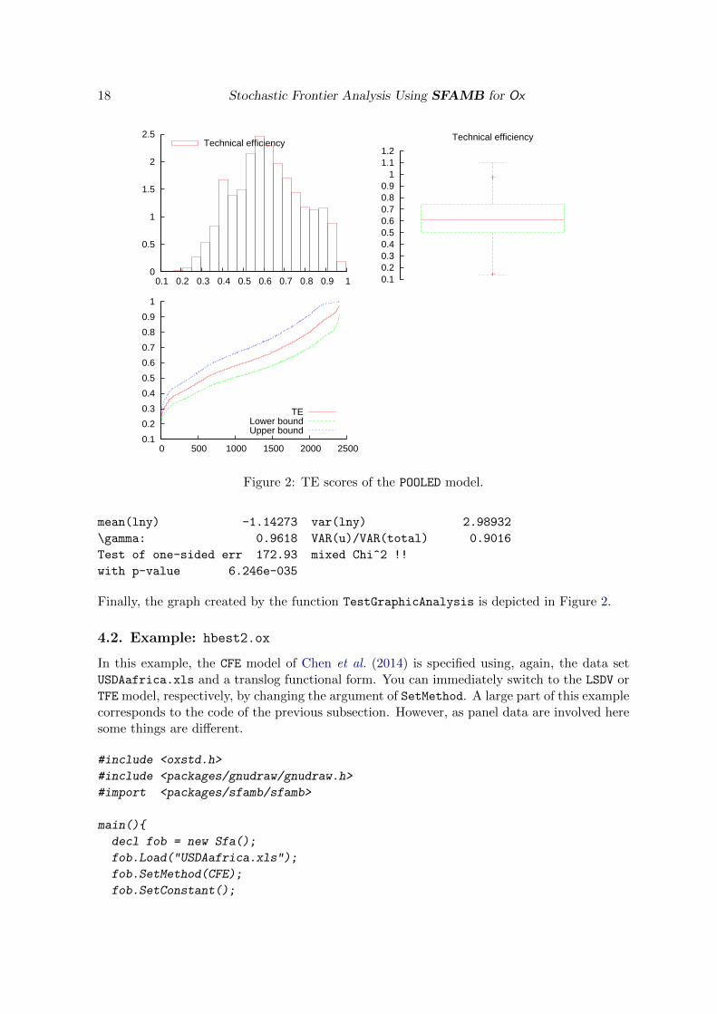
There is a graphical functionality involving the package GnuDraw that allows for a visualassessment of the efficiency scores. The function TestGraphicAnalysis displays the graphicspresented in Figure 2. The confidence band can be changed with SetConfidenceLevel, wherean error probability of 0.05 is the default.

fob.SetConfidenceLevel(0.05);

fob.TestGraphicAnalysis();

The output of this program appears as follows (omitting information on the maximizationprocedure). Some general information:

SFAMB package version 1.1, object created on 19-02-2014

Constructing Squares and Cross-Products...done.

-Pooled model-

---- SFAMB ----

The estimation sample is: 1 - 2400

The dependent variable is: lny

The dataset is: USDAafrica.xls

The transformed variables facilitate the interpretation of the estimated coefficients of thetranslog functional form. Thus, the first order coefficients listed below can be interpreted asoutput elasticities at the sample mean. These estimates are positive and meet the requirementof monotonicity – except for the machinery input whose (insignificant) estimate violates theregularity condition. The parameter associated with trend indicates the estimated averagerate of technical change per year.

Coefficient Std.Error robust-SE t-value t-prob

Constant 0.418510 0.01734 0.01604 26.1 0.000

lnlab 0.128543 0.01338 0.01105 11.6 0.000

lnland 0.747665 0.01552 0.01301 57.5 0.000

lnmac -0.0103601 0.009487 0.008851 -1.17 0.242

lnfert 0.0753082 0.006573 0.006243 12.1 0.000

trend 0.0104214 0.0007006 0.0006763 15.4 0.000

Furthermore, the output shows the coefficients of the squared and cross terms that can beused to calculate the individual output elasticities.

Coefficient Std.Error robust-SE t-value t-prob

.5*lnlab^2 -0.0555284 0.02432 0.02387 -2.33 0.020

Journal of Statistical Software 17

.5*lnland^2 -0.170593 0.02547 0.02843 -6.00 0.000

.5*lnmac^2 -0.0152333 0.005151 0.004632 -3.29 0.001

.5*lnfert^2 0.0611977 0.003107 0.003063 20.0 0.000

.5*trend^2 0.000420193 6.481e-005 6.132e-005 6.85 0.000

lnlab*lnland 0.189011 0.02492 0.02557 7.39 0.000

lnlab*lnmac -0.125612 0.008138 0.007344 -17.1 0.000

lnlab*lnfert -0.0294981 0.006109 0.005248 -5.62 0.000

lnlab*trend -0.000443318 0.0007217 0.0006231 -0.711 0.477

lnland*lnmac 0.137893 0.008829 0.008381 16.5 0.000

lnland*lnfert -0.0633867 0.006748 0.006383 -9.93 0.000

lnland*trend -0.000495235 0.0007838 0.0007483 -0.662 0.508

lnmac*lnfert -0.0135746 0.002997 0.002857 -4.75 0.000

lnmac*trend 0.000810357 0.0002892 0.0002743 2.95 0.003

lnfert*trend 0.000898471 0.0002366 0.0002062 4.36 0.000

After the technology parameters, the estimates of σv and σu are listed in the form of theirnatural logarithms. The next line refers to the noise component.

Coefficient Std.Error robust-SE t-value t-prob

ln{\sigma_v} -2.64681 0.1459 0.1361 -19.4 0.000

Since ln (σu) is parameterized using covariates, there are several related estimates. The orderof coefficients corresponds to the specification ln (σu) = δ0 +

∑4l=1 δl× zl where l = 1 (labor),

2 (land), 3 (machinery), 4 (fertilizer); and the z ’s are in logarithms. Higher use of zl isassociated with a lower level of inefficiency (or higher technical efficiency) if the estimatedparameter has a negative sign.

Coefficient Std.Error robust-SE t-value t-prob

Constant -1.04439 0.04104 0.04790 -21.8 0.000

lnlab 0.232702 0.04300 0.05044 4.61 0.000

lnland -0.146200 0.04176 0.05050 -2.90 0.004

lnmac -0.00976576 0.01491 0.01671 -0.584 0.559

lnfert -0.0149142 0.01372 0.01647 -0.905 0.365

Here, the inefficiency distribution is supposed to have a non-zero mean, ui ∼ N+(µ = µ0, σ2u,i),

i.e., the location parameter is a constant (µ0) common to all individuals. Additional covariatescould be introduced. The omission of U_VAR in the model specification leads to µ = 0, andhence, results in the normal half-normal model. Note that this estimate (here, the thirdConstant) is always the last Constant term in the list (if a truncated-normal is specified).

Coefficient Std.Error robust-SE t-value t-prob

Constant 0.454144 0.02926 0.03249 14.0 0.000

Some additional information is provided, for details see Section 3.3.

log-likelihood -458.928611

no. of observations 2400 no. of parameters 28

AIC.T 973.857222 AIC 0.405773842

18 Stochastic Frontier Analysis Using SFAMB for Ox

0

0.5

1

1.5

2

2.5

0.1 0.2 0.3 0.4 0.5 0.6 0.7 0.8 0.9 1

Technical efficiency

0.1 0.2 0.3 0.4 0.5 0.6 0.7 0.8 0.9

1 1.1 1.2

Technical efficiency

0.1

0.2

0.3

0.4

0.5

0.6

0.7

0.8

0.9

1

0 500 1000 1500 2000 2500

TELower boundUpper bound

Figure 2: TE scores of the POOLED model.

mean(lny) -1.14273 var(lny) 2.98932

\gamma: 0.9618 VAR(u)/VAR(total) 0.9016

Test of one-sided err 172.93 mixed Chi^2 !!

with p-value 6.246e-035

Finally, the graph created by the function TestGraphicAnalysis is depicted in Figure 2.

4.2. Example: hbest2.ox

In this example, the CFE model of Chen et al. (2014) is specified using, again, the data setUSDAafrica.xls and a translog functional form. You can immediately switch to the LSDV orTFE model, respectively, by changing the argument of SetMethod. A large part of this examplecorresponds to the code of the previous subsection. However, as panel data are involved heresome things are different.

#include <oxstd.h>

#include <packages/gnudraw/gnudraw.h>

#import <packages/sfamb/sfamb>

main(){

decl fob = new Sfa();

fob.Load("USDAafrica.xls");

fob.SetMethod(CFE);

fob.SetConstant();

Journal of Statistical Software 19

CFE is the estimator selected. Here, the function SetConstant does not create a constantbecause it is not required. However, this line can be kept for convenience. The functionIdent identifies the panel structure of the data. The required information includes the variablenames of the individuals ("ID") and the period ("time").

fob.Ident(fob.GetVar("ID"), fob.GetVar("time"));

Data transformation and model specification correspond to the previous example. Note thatneither U_VAR nor Z_VAR are available here.

decl inorm = 1;

fob.Renew(fob.PrepData(fob.GetVar("output"), inorm), "lny");

fob.Renew(fob.PrepData(fob.GetVar("labour"), inorm), "lnlab");

fob.Renew(fob.PrepData(fob.GetVar("land"), inorm), "lnland");

fob.Renew(fob.PrepData(fob.GetVar("machinery"), inorm), "lnmac");

fob.Renew(fob.PrepData(fob.GetVar("fertilizer"), inorm), "lnfert");

fob.Renew(fob.GetVar("time") - meanc(fob.GetVar("time")), "trend");

fob.Select(Y_VAR, {"lny", 0, 0});

fob.Select(X_VAR, {

"Constant", 0, 0,

"lnlab", 0, 0,

"lnland", 0, 0,

"lnmac", 0, 0,

"lnfert", 0, 0,

"trend", 0, 0});

fob.SetSelSample(-1, 1, -1, 1);

fob.SetPrintSfa(TRUE);

MaxControl(1000, 10, TRUE);

fob.SetTranslog(1);

fob.Estimate();

For this model, there is no calculation of the confidence bounds involved. The efficiency scorescan be extracted as point estimates using function TE.

fob.Renew(fob.TE(), {"TE"});

fob.Renew(fob.Ineff(), {"jlms"});

fob.TestGraphicAnalysis();

delete fob;

}

The output of this program appears as follows. Additional information on the panel structureis printed.

SFAMB package version 1.1, object created on 19-02-2014

#groups: #periods(max): avg.T-i:

20 Stochastic Frontier Analysis Using SFAMB for Ox

48.000 50.000 50.000

Constructing Squares and Cross-Products...done.

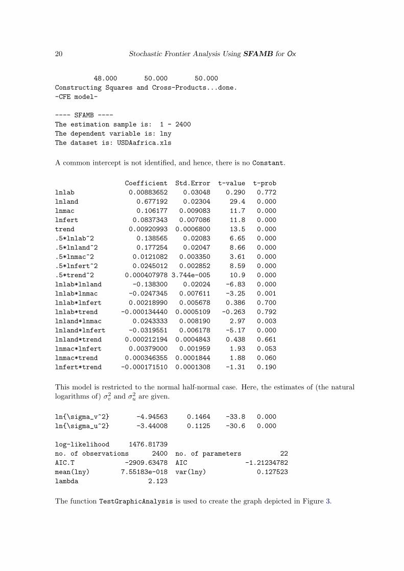
-CFE model-

---- SFAMB ----

The estimation sample is: 1 - 2400

The dependent variable is: lny

The dataset is: USDAafrica.xls

A common intercept is not identified, and hence, there is no Constant.

Coefficient Std.Error t-value t-prob

lnlab 0.00883652 0.03048 0.290 0.772

lnland 0.677192 0.02304 29.4 0.000

lnmac 0.106177 0.009083 11.7 0.000

lnfert 0.0837343 0.007086 11.8 0.000

trend 0.00920993 0.0006800 13.5 0.000

.5*lnlab^2 0.138565 0.02083 6.65 0.000

.5*lnland^2 0.177254 0.02047 8.66 0.000

.5*lnmac^2 0.0121082 0.003350 3.61 0.000

.5*lnfert^2 0.0245012 0.002852 8.59 0.000

.5*trend^2 0.000407978 3.744e-005 10.9 0.000

lnlab*lnland -0.138300 0.02024 -6.83 0.000

lnlab*lnmac -0.0247345 0.007611 -3.25 0.001

lnlab*lnfert 0.00218990 0.005678 0.386 0.700

lnlab*trend -0.000134440 0.0005109 -0.263 0.792

lnland*lnmac 0.0243333 0.008190 2.97 0.003

lnland*lnfert -0.0319551 0.006178 -5.17 0.000

lnland*trend 0.000212194 0.0004843 0.438 0.661

lnmac*lnfert 0.00379000 0.001959 1.93 0.053

lnmac*trend 0.000346355 0.0001844 1.88 0.060

lnfert*trend -0.000171510 0.0001308 -1.31 0.190

This model is restricted to the normal half-normal case. Here, the estimates of (the naturallogarithms of) σ2v and σ2u are given.

ln{\sigma_v^2} -4.94563 0.1464 -33.8 0.000

ln{\sigma_u^2} -3.44008 0.1125 -30.6 0.000

log-likelihood 1476.81739

no. of observations 2400 no. of parameters 22

AIC.T -2909.63478 AIC -1.21234782

mean(lny) 7.55183e-018 var(lny) 0.127523

lambda 2.123

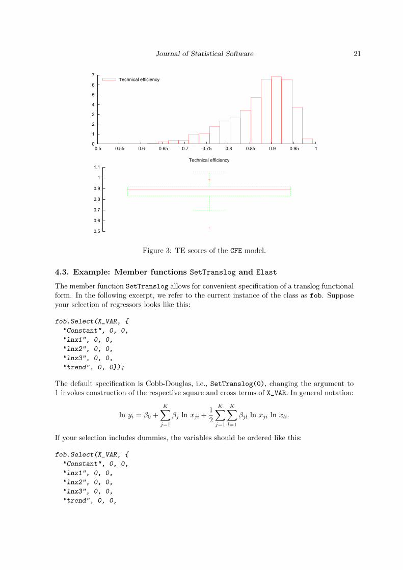
The function TestGraphicAnalysis is used to create the graph depicted in Figure 3.

Journal of Statistical Software 21

0

1

2

3

4

5

6

7

0.5 0.55 0.6 0.65 0.7 0.75 0.8 0.85 0.9 0.95 1

Technical efficiency

0.5

0.6

0.7

0.8

0.9

1

1.1

Technical efficiency

Figure 3: TE scores of the CFE model.

4.3. Example: Member functions SetTranslog and Elast

The member function SetTranslog allows for convenient specification of a translog functionalform. In the following excerpt, we refer to the current instance of the class as fob. Supposeyour selection of regressors looks like this:

fob.Select(X_VAR, {

"Constant", 0, 0,

"lnx1", 0, 0,

"lnx2", 0, 0,

"lnx3", 0, 0,

"trend", 0, 0});

The default specification is Cobb-Douglas, i.e., SetTranslog(0), changing the argument to1 invokes construction of the respective square and cross terms of X_VAR. In general notation:

ln yi = β0 +

K∑j=1

βj ln xji +1

2

K∑j=1

K∑l=1

βjl ln xji ln xli.

If your selection includes dummies, the variables should be ordered like this:

fob.Select(X_VAR, {

"Constant", 0, 0,

"lnx1", 0, 0,

"lnx2", 0, 0,

"lnx3", 0, 0,

"trend", 0, 0,

22 Stochastic Frontier Analysis Using SFAMB for Ox

"dummy1", 0, 0,

"dummy2", 0, 0});

Specification of a translog form is then possible by means of SetTranslog(4) because onlythe first four regressors are used ("Constant" is ignored automatically).

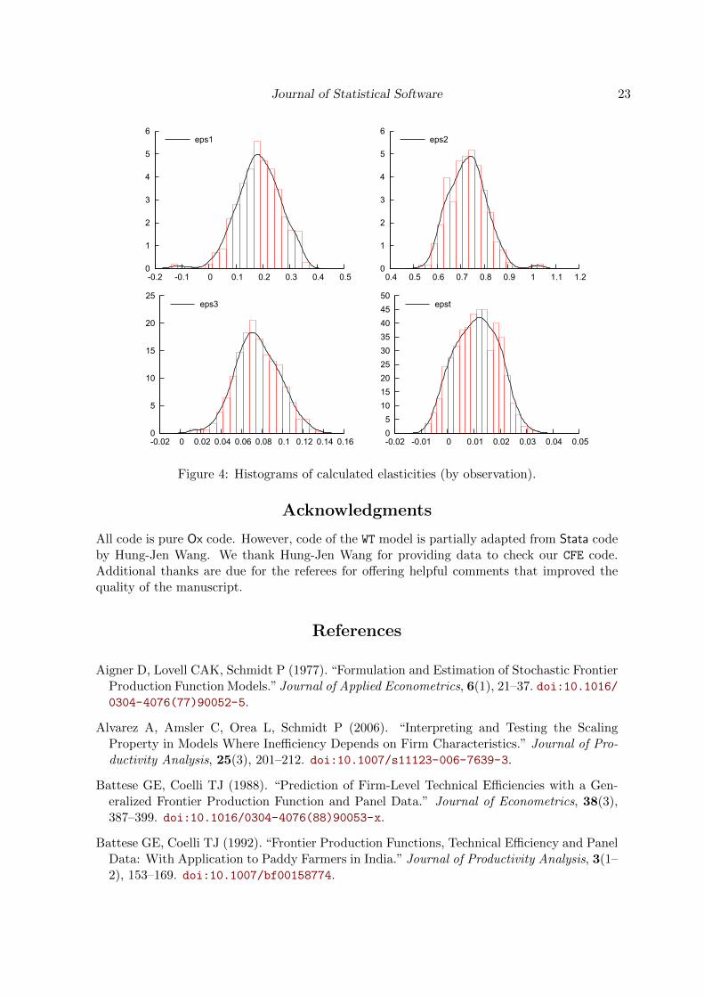
After estimation, the member function Elast can be used to calculate the output elasticity(εji) of each input for each observation:

εji = βj +K∑l=1

βjl ln xli.

The following example illustrates one possible way the function may be used. Here, resultsare plotted as histograms (see Figure 4). Note that indexing starts at 0 in Ox (Elast returnsan NT × 2 matrix but only the first column is considered here). The first three argumentsof DrawDensity are the most important here: area (panel) index, variable, label. See thedocumentations of Ox or GnuDraw for a full description.

decl vEps1 = fob.Elast("lnx1");

decl vEps2 = fob.Elast("lnx2");

decl vEps3 = fob.Elast("lnx3");

decl vEpst = fob.Elast("trend");

DrawDensity(0, vEps1[][0]', {"eps1"}, 1, 1, 0, 0, 0, 0, 1, 0, 1);

DrawDensity(1, vEps2[][0]', {"eps2"}, 1, 1, 0, 0, 0, 0, 1, 0, 1);

DrawDensity(2, vEps3[][0]', {"eps3"}, 1, 1, 0, 0, 0, 0, 1, 0, 1);

DrawDensity(3, vEpst[][0]', {"epst"}, 1, 1, 0, 0, 0, 0, 1, 0, 1);

ShowDrawWindow();

5. Future developments

The basic version of SFAMB dates back to the mid 1990s where the capability was restrictedto cross-sectional data. As the package now allows for panel data and the literature on SFmethods is considerably broader and still growing, there is scope for potential extensions.Some related possibilities are mentioned here.

In the model framework of Chen et al. (2014) there are two ways to calculate the individualeffects. As an alternative to Equation 5, the individual “between estimator of αi” can beused. It could be implemented as an optional function, involving a second maximization. Itsavailability would allow us to compare results and check the consequences for TE scores.

While the current focus of panel methods is on fixed effects estimation, a more comprehen-sive supplement might involve random effects models. The most recent SF approach usingthe CSN distribution is presented by Colombi, Kumbhakar, Martini, and Vittadini (2014).Its specification is similar to Equation 3, but the time-invariant part is further decomposedinto two residuals (persistent inefficiency and time-invariant unobserved heterogeneity). Fil-ippini and Greene (2016) introduce computational simplifications and label the model as the“Generalized True Random Effects SF model”.

Journal of Statistical Software 23

0

1

2

3

4

5

6

-0.2 -0.1 0 0.1 0.2 0.3 0.4 0.5

eps1

0

1

2

3

4

5

6

0.4 0.5 0.6 0.7 0.8 0.9 1 1.1 1.2

eps2

0

5

10

15

20

25

-0.02 0 0.02 0.04 0.06 0.08 0.1 0.12 0.14 0.16

eps3

0

5

10

15

20

25

30

35

40

45

50

-0.02 -0.01 0 0.01 0.02 0.03 0.04 0.05

epst

Figure 4: Histograms of calculated elasticities (by observation).

Acknowledgments

All code is pure Ox code. However, code of the WT model is partially adapted from Stata codeby Hung-Jen Wang. We thank Hung-Jen Wang for providing data to check our CFE code.Additional thanks are due for the referees for offering helpful comments that improved thequality of the manuscript.

References

Aigner D, Lovell CAK, Schmidt P (1977). “Formulation and Estimation of Stochastic FrontierProduction Function Models.” Journal of Applied Econometrics, 6(1), 21–37. doi:10.1016/0304-4076(77)90052-5.

Alvarez A, Amsler C, Orea L, Schmidt P (2006). “Interpreting and Testing the ScalingProperty in Models Where Inefficiency Depends on Firm Characteristics.” Journal of Pro-ductivity Analysis, 25(3), 201–212. doi:10.1007/s11123-006-7639-3.

Battese GE, Coelli TJ (1988). “Prediction of Firm-Level Technical Efficiencies with a Gen-eralized Frontier Production Function and Panel Data.” Journal of Econometrics, 38(3),387–399. doi:10.1016/0304-4076(88)90053-x.

Battese GE, Coelli TJ (1992). “Frontier Production Functions, Technical Efficiency and PanelData: With Application to Paddy Farmers in India.” Journal of Productivity Analysis, 3(1–2), 153–169. doi:10.1007/bf00158774.

24 Stochastic Frontier Analysis Using SFAMB for Ox

Battese GE, Coelli TJ (1995). “A Model for Technical Inefficiency Effects in a StochasticFrontier Production Function for Panel Data.” Empirical Economics, 20(2), 325–332. doi:10.1007/bf01205442.

Battese GE, Corra GS (1977). “Estimation of a Production Function Model: With Applicationto the Pastoral Zone of Eastern Australia.” Australian Journal of Agricultural Economics,21(3), 169–179. doi:10.1111/j.1467-8489.1977.tb00204.x.

Belotti F, Daidone S, Ilardi G, Atella V (2013). “Stochastic Frontier Analysis Using Stata.”Stata Journal, 13(4), 719–758. URL http://www.stata-journal.com/article.html?

article=st0315.

Bogetoft P, Otto L (2010). Benchmarking with DEA, SFA, and R, volume 157 of InternationalSeries in Operations Research & Management Science. Springer-Verlag.

Bos CS (2014). GnuDraw – An Ox Package for Creating gnuplot Graphics. URL http:

//personal.vu.nl/c.s.bos/software/gnudraw.html.

Brorsen BW, Kim T (2013). “Data Aggregation in Stochastic Frontier Models: The ClosedSkew Normal Distribution.” Journal of Productivity Analysis, 39(1), 27–34. doi:10.1007/s11123-012-0274-2.

Brummer B (2001). “Estimating Confidence Intervals for Technical Efficiency: The Case ofPrivate Farms in Slovenia.” European Review of Agricultural Economics, 28(3), 285–306.doi:10.1093/erae/28.3.285.

Caudill SB, Ford JM, Gropper DM (1995). “Frontier Estimation and Firm-Specific InefficiencyMeasures in the Presence of Heteroscedasticity.” Journal of Business & Economic Statistics,13(1), 105–111. doi:10.2307/1392525.

Chen YY, Schmidt P, Wang HJ (2014). “Consistent Estimation of the Fixed Effects StochasticFrontier Model.” Journal of Econometrics, 181(2), 65–76. doi:10.1016/j.jeconom.2013.05.009.

Coelli TJ (1996). A Guide to FRONTIER 4.1: A Computer Program for Stochastic FrontierProduction and Cost Function Estimation. CEPA Working Papers, University of NewEngland, URL http://www.uq.edu.au/economics/cepa/frontier.php.

Coelli TJ, Henningsen A (2017). frontier: Stochastic Frontier Analysis. R package version1.1-2, URL https://CRAN.R-Project.org/package=frontier.

Coelli TJ, Rao PDS, O’Donnell CJ, Battese GE (2005). An Introduction to Efficiency andProductivity Analysis. Springer-Verlag. doi:10.1007/978-1-4615-5493-6.

Colombi R, Kumbhakar SC, Martini G, Vittadini G (2014). “Closed-Skew Normality inStochastic Frontiers with Individual Effects and Long/Short-Run Efficiency.” Journal ofProductivity Analysis, 42(2), 123–136. doi:10.1007/s11123-014-0386-y.

Cottrell A, Lucchetti R (2014). gretl User’s Guide – Gnu Regression, Econometrics andTime-Series Library. URL http://gretl.sourceforge.net/.

Journal of Statistical Software 25

Doornik JA (2009). An Object-Oriented Matrix Language Ox 6. Timberlake ConsultantsPress, London.

Doornik JA, Ooms M (2007). Introduction to Ox: An Object-Oriented Matrix Language. Tim-berlake Consultants Press, London. Available at http://www.doornik.com/ox/OxIntro.

pdf.

Econometric Software Inc (2014). LIMDEP, Version 10.0. ESI, New York. URL http:

//www.limdep.com/.

Filippini M, Greene WH (2016). “Persistent and Transient Productive Inefficiency: A Max-imum Simulated Likelihood Approach.” Journal of Productivity Analysis, 45(2), 187–196.doi:10.1007/s11123-015-0446-y.

Fuglie KO (2012). “Productivity Growth and Technology Capital in the Global AgriculturalEconomy.” In KO Fuglie, SL Wang, VE Ball (eds.), Productivity Growth in Agriculture:An International Perspective. CABI.

gnuplot Team (2015). gnuplot 5.0 – An Interactive Plotting Program. URL http:

//sourceforge.net/projects/gnuplot.

Greene WH (2005). “Reconsidering Heterogeneity in Panel Data Estimators of the StochasticFrontier Model.” Journal of Econometrics, 126(2), 269–303. doi:10.1016/j.jeconom.

2004.05.003.

Greene WH (2008). “The Econometric Approach to Efficiency Analysis.” In HO Fried,CAK Lovell, SS Schmidt (eds.), The Measurement of Productive Efficiency and Produc-tivity Growth. Oxford University Press.

Greene WH (2012). Econometric Analysis. 7th edition. Pearson International Edition.

Horrace WC, Schmidt P (1996). “Confidence Statements for Efficiency Estimates fromStochastic Frontier Models.” Journal of Productivity Analysis, 7(2–3), 257–282. doi:

10.1007/bf00157044.

Huang CJ, Liu JT (1994). “Estimation of a Non-Neutral Stochastic Frontier ProductionFunction.” Journal of Productivity Analysis, 5(2), 171–180. doi:10.1007/bf01073853.

Hughes G (2008). sfa hetmod and sfa mod. User-Contributed Function Pack-ages for gretl. URL https://gretlwiki.econ.univpm.it/wiki/index.php/List_of_

available_user-contributed_function_packages.

Jondrow J, Lovell CAK, Materov IS, Schmidt P (1982). “On the Estimation of Technical In-efficiency in the Stochastic Frontier Production Function Model.” Journal of Econometrics,19(2–3), 233–238. doi:10.1016/0304-4076(82)90004-5.

Kodde DA, Palm FC (1986). “Wald Criteria for Jointly Testing Equality and InequalityRestrictions.” Econometrica, 54(5), 1243–1248. doi:10.2307/1912331.

Kotz S, Balakrishnan N, Johnson NL (2000). Continuous Multivariate Distributions: Modelsand Applications, volume 1. John Wiley & Sons. doi:10.1002/0471722065.

26 Stochastic Frontier Analysis Using SFAMB for Ox

Kumbhakar SC, Gosh S, McGuckin JT (1991). “A Generalized Production Frontier Approachfor Estimating Determinants of Inefficiency in U.S. Dairy Farms.” Journal of Business &Economic Statistics, 9(3), 279–286. doi:10.2307/1391292.

Kumbhakar SC, Lovell CAK (2000). Stochastic Frontier Analysis. Cambridge UniversityPress, Cambridge.

Lai H, Huang CJ (2010). “Likelihood Ratio Tests for Model Selection of Stochas-tic Frontier Models.” Journal of Productivity Analysis, 34(1), 3–13. doi:10.1007/

s11123-009-0160-8.

Meeusen W, Van den Broeck J (1977). “Efficiency Estimation from Cobb-Douglas ProductionFunctions with Composed Error.” International Economic Review, 18(2), 435–444. doi:

10.2307/2525757.

Pavlyuk D (2016). spfrontier: Spatial Stochastic Frontier Models Estimation. R packageversion 0.2.3, URL https://CRAN.R-project.org/package=spfrontier.

Piessens R, de Doncker-Kapenga E, Uberhuber CW, Kahaner DK (1983). QUADPACK,A Subroutine Package for Automatic Integration. Springer-Verlag.

R Core Team (2017). R: A Language and Environment for Statistical Computing. R Founda-tion for Statistical Computing, Vienna, Austria. URL https://www.R-project.org/.

Reifschneider D, Stevenson R (1991). “Systematic Departures from the Frontier: A Frameworkfor the Analysis of Firm Inefficiency.” International Economic Review, 32(3), 715–723.doi:10.2307/2527115.

Schmidt P, Sickles RC (1984). “Production Frontiers and Panel Data.” Journal of Business& Economic Statistics, 2(4), 367–374. doi:10.2307/1391278.

StataCorp LP (2015). Stata, Version 14. College Station. URL http://www.stata.com/.

Wang HJ (2012). Manual of Hung-Jen Wang’s Stata Codes. URL http://homepage.ntu.

edu.tw/~wangh.

Wang HJ, Ho CW (2010). “Estimating Fixed-Effect Panel Stochastic Frontier Models byModel Transformation.” Journal of Econometrics, 157(2), 286–296. doi:10.1016/j.

jeconom.2009.12.006.

Wang HJ, Schmidt P (2002). “One-Step and Two-Step Estimation of the Effects of ExogenousVariables on Technical Efficiency Levels.” Journal of Productivity Analysis, 18(2), 129–144.doi:10.1023/a:1016565719882.

White H (1980). “A Heteroskedasticity-Consistent Covariance Matrix Estimator and a DirectTest for Heteroskedasticity.” Econometrica, 48(4), 817–838. doi:10.2307/1912934.

Journal of Statistical Software 27

A. Technical appendix

A.1. Starting values

OLS estimates are used as starting values for the technology parameters β, and a grid searchis applied to find an appropriate value for σ2 = σ2v + σ2u. Battese and Corra (1977, p. 173)point out that the OLS estimates of β are unbiased, except for the common constant β0.They show that β0 can be corrected as:

β0 = βOLS0 +

√2

πσu.

Furthermore, they define γ = σ2u/(σ2v + σ2u), and suggest to try different initial values. The

grid search evaluates the likelihood function over a range of values (γ [0.05, 0.98]) and choosesthe parameters associated with the highest likelihood value. Within this procedure, σ2v andσ2u are parameterized as:15

σ2v = σ2 × (1− γ) =(σ2v + σ2u

)×(σ2v + σ2uσ2v + σ2u

− σ2uσ2v + σ2u

),

σ2u = σ2 × γ =(σ2v + σ2u

)× σ2uσ2v + σ2u

.

The search for values for σ2v and σ2u involves partitioning the variance of the composed errorterm. Aigner et al. (1977) show that VAR(ε) = σ2v + ((π − 2)/π)σ2u, which can be expressedas:

VAR(ε) = σ2(1− γ) +π − 2

πσ2γ = σ2

(1− γ

(1− π − 2

π

)).

Using the variance of the OLS residuals (m2) as an estimate for VAR(ε):

m2 = σ2(

1− γ 2

π

)←→ σ2 =

m2

1− γ 2π

.

The grid search is called within member function DoEstimation, and runs over γ values withstep length 0.01; it passes the starting values for β and σ2 back to DoEstimation.

A.2. Estimation and standard errors

After the starting values are obtained from the OLS regression and grid search, the log-likelihood function is maximized using the BFGS (Broyden-Fletcher-Goldfarb-Shanno) algo-rithm. The respective Ox routine is named MaxBFGS and documented in Doornik (2009) andonline at http://www.doornik.com/ox/. The log-likelihood function can be found as func-tion fSfa in the source code.16 Analytical first derivatives are used in the case of the POOLED

15In case of the pooled model, the parameters are σv and σu. In case of the panel models, there is no constant(β0) to be corrected. If the model includes additional covariates (z-variables, related to inefficiency), a vectorof zeros is used for the respective parameters. Zeros are also used as starting values for the individual effectsin the TFE model.

16Member functions of the source code are structured by case(s) where default = POOLED, 1 = WT, 2 =

LSDV, 3 = CFE, 4 = TFE.

28 Stochastic Frontier Analysis Using SFAMB for Ox

model, while the remaining models employ numerical first derivatives based on the Ox routineNum1Derivative (finite difference approximation).

The CFE model’s “within-likelihood function” includes a T -dimensional cdf. In their Ap-pendix C, Chen et al. (2014) show how the T -dimensional integral is reduced to a one-dimensional integral, referring to Kotz, Balakrishnan, and Johnson (2000) (fKotzetal is therespective function). The numerical quadrature is executed by function QNG which is partof the Fortran package QuadPack (Piessens, de Doncker-Kapenga, Uberhuber, and Kahaner1983) and linked in via #include <quadpack.h>.

Standard errors are obtained from m_mCovar (covariance matrix). This data member is pro-duced by function Num2Derivative (called within member function Covar) that uses a finitedifference approximation (Doornik 2009). Estimation output of the cross-sectional model re-turns robust standard errors (by default) which are obtained by the method of White (1980).

A.3. Log-likelihood functions

In this section, φ and Φ denote the pdf and cdf of a standard normal distribution, respectively;λ = σu/σv and σ2 = σ2u + σ2v .

Kumbhakar and Lovell (2000) present the log-likelihood functions of the normal-truncated

normal model (uiiid∼ N+(µ, σ2u)) and the normal-half normal model (µ = 0) for cross-sectional

data. The log-likelihood function of the POOLED model for one observation, with εi = yi−β>xi,is given by:

ln Li = ln1√2π− 1

2ln σ2 − (εi + µ)2

2σ2+ ln Φ

(µ

σλ− λεi

σ

)− ln Φ

(µ

√1 + λ2

σλ

). (6)

The log-likelihood function of the TFE model (Greene 2005) corresponds to Equation 6, butwith µ = 0 and εit = yit − β>xit − αi in the place of εi.

The log-likelihood function of the WT model (Wang and Ho 2010) for one individual, withεit = yit − β>xit, and εi = (εi1, . . . , εiT )>:

ln Li = −1

2(T − 1) ln(2π)− 1

2(T − 1) ln(σ2v)−

1

2ε>i Π−εi

+1

2

(µ2∗∗σ2∗∗− µ2

σ2u

)+ ln

(σ∗∗Φ

(µ∗∗σ∗∗

))− ln

(σuΦ

(µ

σu

)),

where

µ∗∗ =µ/σ2u − ε>i Π−hi

h>i Π−hi + 1/σ2u

,

σ2∗∗ =1

h>i Π−hi + 1/σ2u

.

Log-likelihood function of the CFE model (Chen et al. 2014), with εit = yit − β>xit, εi =

Journal of Statistical Software 29

(εi1, . . . , εiT )>, and ε∗i = (εi1, . . . , εi,T−1)>:

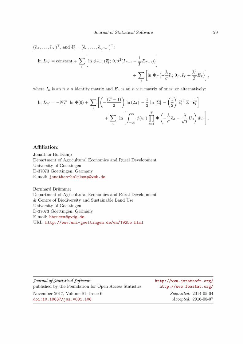
ln LW = constant +∑i

[ln φT−1 (ε∗i ; 0, σ2(IT−1 −

1

TET−1))

]+∑i

[ln ΦT (−λ

σεi; 0T , IT +

λ2

TET )

],

where In is an n× n identity matrix and En is an n× n matrix of ones; or alternatively:

ln LW = −NT ln Φ(0) +∑i

[(−(T − 1)

2

)ln (2π) − 1

2ln |Σ| −

(1

2

)ε∗>i Σ− ε∗i

]

+∑i

ln

[∫ ∞−∞

φ(u0)T∏t=1

Φ

(−λσεit −

λ√TU0

)du0

].

Affiliation:

Jonathan HoltkampDepartment of Agricultural Economics and Rural DevelopmentUniversity of GoettingenD-37073 Goettingen, GermanyE-mail: jonathan-holtkamp@web.de

Bernhard BrummerDepartment of Agricultural Economics and Rural Development& Centre of Biodiversity and Sustainable Land UseUniversity of GoettingenD-37073 Goettingen, GermanyE-mail: bbruemm@gwdg.deURL: http://www.uni-goettingen.de/en/19255.html

Journal of Statistical Software http://www.jstatsoft.org/

published by the Foundation for Open Access Statistics http://www.foastat.org/

November 2017, Volume 81, Issue 6 Submitted: 2014-05-04doi:10.18637/jss.v081.i06 Accepted: 2016-08-07