Stochastic Frontier Analysis

Tristan D. Skolrud

EconS 504/EconS 513

March 21, 2016

Part 1

Aigner, D., C. A. Lovell, P. Schmidt. 1977. Formulation andEstimation of Stochastic Frontier Production Models. Journal ofEconometrics(6) 21-37.

ALS

Introduction

I Prior to ALS (Aigner, Lovell, and Schmidt 1977) and MvdB(Meeusen and Van den Broeck 1977), the estimation ofparametric production functions started with the theoreticalrepresentation of a production function

yi = f (xi , β)

where yi represents the maximal amount of output yiobtainable from inputs xi and production technology f (xi , β)

SFA 504/513

ALS

I Estimation followed mathematical programming techniques(Aigner and Chu 1968), maximizing

n∑i=1

(yi − f (xi , β))

orn∑

i=1

(yi − f (xi , β))2

s.t. yi ≤ f (xi , β).

Raises two questions:

1. How does one explain differences in yi for identical xi?

2. What accounts for a firm producing below (or above) thef (xi , β) frontier?

SFA 504/513

ALS

I Answer: Measurement error

I But this fails to address the stochastic nature of production,long realized by economists and highlighted by the pioneeringtheoretical work of Farrell (1957).

I ALS and MvdB sought to operationalize the theoreticalframework of Farrell (1957), allowing for the estimation of astochastic production frontier, where firms could operatebelow the frontier for two reasons:

1. Technical inefficiency2. Statistical noise (measurement error)

I How is technical inefficiency defined?

SFA 504/513

ALS

Technical InefficiencyIntuitively, technical inefficiency is the amount by which all inputscan be proportionally reduced without a reduction in output

[Graph]

SFA 504/513

ALS

Stochastic FrontierWith the idea of technical inefficiency in mind, consider thefollowing parametric equation:

yi = f (xi , β) + εi

where εi = vi − ui for i = 1, . . . n (firms) and

I vi is a symmetric error term accounting for statistical noise

I ui is a non-negative term accounting for technical inefficiency

Each firm’s output must lie on or below its frontier,yi ≤ f (xi , β) + vi , which can vary randomly across firms or overtime.

SFA 504/513

ALS

Checking for the initial presence of TE

I Observe that if ui = 0, then εi = vi , implying that the errorterm is symmetric, which does not support the presence oftechnical inefficiency

I However, if ui > 0, then εi should be negatively skewed

I SFA should start with a simple test (Schmidt and Lin 1984) ofthe presence of TE in the data. Consider the test statistic:

(b1)(1/2) =m3

(m2)(3/2)

where m2 and m3 are the second and third sample momentsof the OLS residuals of the previous model. m3 < 0 indicatestechnical efficiency may be present, and m3 > 0 is a sign thatyour model may be misspecified.

SFA 504/513

ALS

Checking for the initial presence of TEAs a quick note, the distribution for (b1)(1/2) is not widelydistributed, so it’s more common to test the statistic:

balt =m3

(6m32/n)1/2

∼ N(0, 1)

SFA 504/513

ALS

EstimationMaximum likelihood is the preferred technique, representing anincrease in efficiency over OLS. Of course, that means we require avariety of assumptions about the standard errors:

E (vi ) = 0

E (v2i ) = σ2v

E (vivj) = 0 for all i 6= j

E (u2i ) = constant

E (uiuj) = 0 for all i 6= j

(“Corrected” OLS (COLS), GMM, and Bayesian methods havebeen used as well)

SFA 504/513

ALS

For maximum likelihood, we require parametric assumptions aboutthe two disturbance terms. ALS use a normal distribution for thesymmetric disturbance and a half-normal distribution for thetechnical inefficiency term:

vi ∼iid N(0, σ2v )

ui ∼iid N+(0, σ2u)

Other popular choices for the inefficiency term are:

1. Truncated normal

2. Exponential

3. Gamma

In practice, half-normal is the default choice, and the remainingdistributions are often used as robustness checks

SFA 504/513

ALS

Half-normal density

I Negative values set to zero, postitive values follow theright-half of a normal distribution

SFA 504/513

ALS

Half-normal density

I Note that the parameters µ and σ2 in the half-normaldistribution N+(µ, σ2) are not the mean and variance!

I The density is given by

f (x ;σ) =

√2

σ√π

exp

(− x2

2σ2

)I The mean is

E (x) =σ√

2√π

I The variance is

V (x) = σ2(

1− 2

π

)I And the density has support over all x ∈ [0,∞)

SFA 504/513

ALS

ReparameterizationReparameterize variance terms by defining γ = σ2u/σ

2, whereσ2 = σ2u + σ2v . Benefits:

I Reduces search area of γ, {γ ∈ (0, 1)}I Easy interpretation: γ → 1 implies more of the variation is

attributed to inefficiency, and γ → 0 implies more of thevariation due to statistical noise

SFA 504/513

ALS

LikelihoodWith the reparameterization, Battese and Corra (1977)demonstrate that the log-likelihood function can be written:

lnL = −n

2ln(π

2

)− n

2ln(σ2)+

n∑i=1

ln(1−Φ(zi ))− 1

2σ2

n∑i=1

(yi−xiβ)2

where

zi =yi − xiβ

σ

√γ

1− γ

Recall the rule that the density of a sum of random variables, f (z),where Z = X + Y and f (x) and g(y) are the resp. densities, isgiven by the convolution

(f ∗ g)(z) =

∫ ∞−∞

f (z − y)g(y)dy

SFA 504/513

ALS

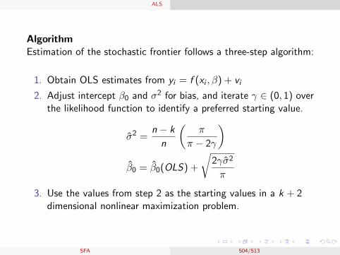
AlgorithmEstimation of the stochastic frontier follows a three-step algorithm:

1. Obtain OLS estimates from yi = f (xi , β) + vi

2. Adjust intercept β0 and σ2 for bias, and iterate γ ∈ (0, 1) overthe likelihood function to identify a preferred starting value.

σ̂2 =n − k

n

(π

π − 2γ

)β̂0 = β̂0(OLS) +

√2γσ̂2

π

3. Use the values from step 2 as the starting values in a k + 2dimensional nonlinear maximization problem.

SFA 504/513

ALS

Firm-Level Technical Efficiency EstimatesMost common output oriented measure of technical efficiency isthe ratio of observed output to the corresponding stochasticfrontier output (Coelli et al. 2005):

TEi =qi

f (xi , β) + vi=

f (xi , β) + vi − uif (xi , β) + vi

When the dependent variable is logged (CD, TL)*, TEi reduces tothe convenient:

TEi = exp(−ui )

*I am unaware of any study that does not utilize a loggeddependent variable in SFA

SFA 504/513

ALS

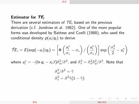
Estimator for TEi

There are several estimators of TEi based on the previousderivation (c.f. Jondrow et al. 1982). One of the more popularforms was developed by Battese and Coelli (1988), who used theconditional density p(ui |qi ) to derive

T̂E i = E (exp(−ui )|qi ) =

[Φ

(u∗iσ∗− σ∗

)/

(u∗iσ∗

)]exp

(σ2∗2− u∗i

)where u∗i = −(ln qi − xiβ)σ̂2u/σ̂

2, and σ̂2∗ = σ̂2v σ̂2u/σ̂

2. Note that

σ̂2u/σ̂2 = γ̂

σ̂2∗ = σ̂2γ̂(1− γ̂)

SFA 504/513

Part 2

Key, Nigel and Stacy Sneeringer. 2014. Potential Effects ofClimate Change on the Productivity of U.S. Dairies. Journal ofEconometrics(6) 21-37.

ALS

Introduction

I The true nature of production is stochastic, especially inagriculture

I The authors suspect that increased instances of drought,higher average temperatures, and hotter daily maximums maybe decreasing technical efficiency in livestock operations,particularly dairies

I The authors specify a model wherein technical efficiency anda vector of variables suspected to influence technical efficiency(associated with climate) are estimated simultaneously

I Results indicate that a one unit increase in the annual THI(temperature-humidity index) load is associated with a 3.7percent reduction in output

I The question for us is: how did they figure this out?

SFA 504/513

ALS

Estimation Strategy

I Objective: Estimate the impact of THI load on technicalefficiency

I Starting point: ALS (1977)/MvdB(1977)

ln(qi ) = f (xi , β) + vi − ui

(where f (xi , β) is parameterized as Translog)

I Recall the deterministic frontier is f (xi , β), the stochasticfrontier is f (xi , β) + vi , where vi is a symmetric randomshock, and ui ≥ 0 represents inefficiency

I With a logged dependent variable, technical efficiency isrepresented by

TEi =qi

exp(f (xi , β) + vi= exp(−ui )

which varies between 0 and 1, where TEi = 1 indicatesperfect technical efficiency

SFA 504/513

ALS

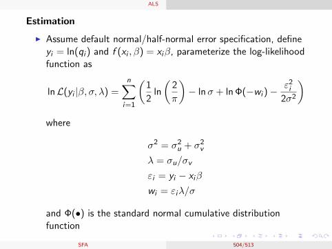
Estimation

I Assume default normal/half-normal error specification, defineyi = ln(qi ) and f (xi , β) = xiβ, parameterize the log-likelihoodfunction as

lnL(yi |β, σ, λ) =n∑

i=1

(1

2ln

(2

π

)− lnσ + ln Φ(−wi )−

ε2i2σ2

)where

σ2 = σ2u + σ2v

λ = σu/σv

εi = yi − xiβ

wi = εiλ/σ

and Φ(•) is the standard normal cumulative distributionfunction

SFA 504/513

ALS

EstimationKey and Sneeringer employ the Jondrow et al. (1982) version ofthe expectation of ui conditional on εi :

E (ui |εi ) =σλ

1 + λ2

(φ(wi )

1− Φ(wi )− wi

)

I With this estimate of ui , how does one calculate the impact ofa set of exogenous factors on its determination?

I Two-step estimation? Just estimate the ui ’s as normal, andthen use it as a dependent variable in a second-stageestimation, regressed on factors thought to have influence

I No. Results in biased and inefficient estimates (Wang andSchmidt 2002)

SFA 504/513

ALS

EstimationA more robust alternative to estimate technical efficiency alongwith the factors that influence it in a single step. To do this:

I Define the variance of the underlying half-normal distributionof ui , σ

2u, as a function of observable factors zu and a set of

parameters δu:σ2ui = exp(zuiδu)

I With this formulation, the factors in zui directly impact themean and variance of the inefficiency term ui , andsubsequently, the estimate of technical efficiency (still useJondrow et al. 1982)

SFA 504/513

ALS

EstimationNote: This formulation increases the dimensionality of thenonlinear maximization problem by the size of the δu vector. Thelikelihood function is now

lnL(yi |β, σ, λ, δu) =n∑

i=1

(1

2ln

(2

π

)− lnσ + ln Φ(−wi )−

ε2i2σ2

)where

σ2 = exp(zuiδu) + σ2v

λ = exp(zuiδu)σv

εi = yi − xiβ

wi = εiλ/σ

SFA 504/513

ALS

What did Key and Sneeringer find?

I Postulated the impact of THI load, operator education,operator age, operator experience, operation size, and ameasure of specialization

I THI = (dry bulb temperature in degrees celsius) + (0.36 xdew point temperature) + 41.2.

I THI load is a measure of the duration and extent above thisthreshold

I Results: THI load has a large, significant impact on technicalefficiency in dairy production. Using 2010 estimates,inefficiency loss from heat stress reduces value byapproximately $1.2 billion/year.

I Climate change simulations: Lost production could get much,much worse depending on the climate simulation model used.

SFA 504/513