a stochastic frontier analysis - eurocontrol
TRANSCRIPT

November 2006
Cost Benchmarking of Air Navigation Service Providers: A Stochastic Frontier Analysis
Final Report

Project Team Stuart Holder Dr. Barbara Veronese Paul Metcalfe Dr. Federico Mini Stewart Carter Bruno Basalisco
NERA Economic Consulting 15 Stratford Place London W1C 1BE United Kingdom Tel: +44 20 7659 8500 Fax: +44 20 7659 8501 www.nera.com

Cost Benchmarking of ANSPs Contents
NERA Economic Consulting
Glossary i
Executive Summary ii
1. Introduction 1
2. Benchmarking Analysis 2 2.1. Background 2 2.2. Benchmarking in Other Industries 4 2.3. Benchmarking Air Navigation Service Provision 5
3. Cost Function for Air Navigation Service Provision 8
3.1. Economic Theory of Costs and Production 8 3.2. Specific Issues Relating to ANSP Cost Benchmarking 9
4. Data Used for the Analysis 15 4.1. Costs 15 4.2. Outputs 17 4.3. Input Prices 18 4.4. Network Size 20 4.5. Traffic Characteristics 21 4.6. Descriptive Statistics 22
5. Econometric Model Specification 28 5.1. ANSP Cost Function 28 5.2. Econometric Estimation Methods 29 5.3. Models for Cross-Sectional Data 29 5.4. Models for Panel Data 30 5.5. Stochastic Frontier Analysis 33
6. Estimation of the Cost Function for ANSPs 37 6.1. Our Approach 37 6.2. Estimation Results 37 6.3. Estimation of Cost Efficiency 41 6.4. Robustness Checks 42
7. Concluding Remarks 43 7.1. Lessons Learnt 43 7.2. Possible Directions for Future Research 43
8. References 47
Cost Benchmarking of ANSPs Contents
NERA Economic Consulting
Appendix A. Economic Theory of Cost Functions 50
Appendix B. Stochastic Frontier Models 52 B.1. Cross Section Specifications 52 B.2. Panel Specifications 53 B.3. Likelihood Functions and Formulae for Estimating
Inefficiency 54
Appendix C. Econometric Estimates from the FE and the RE Time-Varying Models 57
C.1. Main Econometric Estimates 57

Cost Benchmarking of ANSPs Glossary
NERA Economic Consulting i
Glossary
ACC Area Control Centre ACE Air traffic management Cost-Effectiveness Aena Aeropuertos Españoles y Navegación Aérea, Spain ANS Air Navigation Services ANS CR Air Navigation Services of the Czech Republic ANS Sweden ANS department of Swedish Civil Aviation Administration (LFV) ANSP Air Navigation Service Provider APP Approach control unit ATC Air Traffic Control ATCO Air Traffic Control Officer ATFM Air Traffic Flow Management ATM Air Traffic Management ATSA Bulgaria Air Traffic Services Authority, Bulgaria Austro Control Austro Control Österreichische Gesellschaft für Zivilluftfahrt mbH, Austria Avinor Avinor, Norway Belgocontrol Belgocontrol, Belgium COLS Corrected Ordinary Least Squares CNS Communication, Navigation and Surveillance Croatia Control Hrvatska kontrola zračne plovidbe d.o.o., Croatian Air Navigation Services DCAC Cyprus Department of Civil Aviation of Cyprus DEA Data Envelopment Analysis DFS Deutsche Flugsicherung GmbH, Germany DHMİ Devlet Hava Meydanlarι İsletmesi, Turkey DNA Direction de la Navigation Aérienne, France EANS Estonian Air Navigation Services ENAV Ente Nazionale di Assistenza al Volo S.p.A., Italy EU European Union FE Fixed effects Finland CAA Civil Aviation Administration, Finland FYROM Former Yugoslav Republic of Macedonia GDP Gross Domestic Product HCAA Hellenic Civil Aviation Authority, Greece Hungaro Control HungaroControl, Hungary IAA Irish Aviation Authority, Ireland ÍLS Localisers Instrument Landing Systems Localisers LFV Luftfartsverket, Sweden LGS Latvijas Gaisa Satiksme, Latvia LPS Letové Prevádskové Služby Slovenskej Republiky, Státny Podnik, Slovak Republik LVNL Luchtverkeersleiding Nederland, Netherlands MATS Malta Air Traffic Services Ltd MET Aeronautical Meteorology MoldATSA Moldovian Air Traffic Services Authority MUAC Maastricht Upper Air Centre NATA Albania National Air Traffic Agency, Albania NATS National Air Traffic Services, UK NAV Portugal Navegação Aérea de Portugal, EPE NAVIAIR Air Navigation Services – Flyvesikringstjenesten, Denmark OAT Operational Air Traffic OLS Ordinary Least Squares OPS Operations Oro Navigacija State Enterprise Oro Navigacija, Lithuania PRU Performance Review Unit RA Regression analysis RE Random effects ROMATSA Romanian Air Traffic Services Administration SFA Stochastic Frontier Analysis Skyguide Skyguide, Switzerland Slovenia CAA Civil Aviation Authority of the Republic of Slovenia TWR Traffic Control Tower

Cost Benchmarking of ANSPs Executive Summary
NERA Economic Consulting ii
Executive Summary
This report, by NERA Economic Consulting for EUROCONTROL’s Performance Review Unit (PRU), presents the results of an econometric analysis of the costs of air navigation service providers (ANSPs) in Europe. It uses the evidence from four years of annual data submissions (from 2001 to 2004) from 34 ANSPs to examine their relative cost efficiencies. More importantly, it sets out a methodological framework for future studies of ANSP efficiency and identifies possible directions for further research.
Given the constraints of a relatively small dataset, a Cobb-Douglas cost function is used rather than a more flexible (but data-intensive) translog form. To attempt to identify cost inefficiencies, Stochastic Frontier Analysis is applied to Fixed Effects and Random Effects models.
Our preferred specification is a Random Effects time-invariant model, regressing total costs on output, input prices and network size. In general, this produces coefficients that are significant, have the right sign and appear to be robust. However, we believe that the model is likely to overestimate inefficiency, and this is due to the lack of variation within the four year sample period in the exogenous control factors (network size, traffic complexity and seasonal variability) that we include in our analysis. This means that, within a panel data approach, it is difficult to separate the impact of these variables from other differences between ANSPs (including inefficiency). The model estimation is also affected by other problems, including the fact that potential exogenous factors are not identified, and the lack of reliable input price data for direct operating costs (ie non-staff operating costs) and for capital costs.
A larger dataset and more variation in exogenous factors should allow future research to investigate, among other things, new estimation methods and a more flexible functional form. For the benefits of this larger dataset to be realised, however, we believe it would also be useful to investigate alternative measures of input prices for direct operating costs, and also alternative measures of capital inputs and prices.

Cost Benchmarking of ANSPs Introduction
NERA Economic Consulting 1
1. Introduction
This report, by NERA Economic Consulting for EUROCONTROL’s Performance Review Unit (PRU), presents the results of an econometric analysis of the costs of air navigation service providers (ANSPs) in Europe.
Since 2001, all European ANSPs have been required to provide an annual data submission to the PRU, which have provided the basis for the PRU’s annual ATM Cost-Effectiveness (ACE) Benchmarking Reports. These data submissions are intended to provide a robust basis on which to compare the efficiency performance of European ANSPs, and they have been subjected to a process of validation. Data are now available for four years (2001-2004), and these provide most of the inputs for our own analysis.
Our empirical analysis is exploratory. We examine what the data available at present can tell us about the nature of ANSP costs (for example, the main cost drivers, the existence of economies of scale or density, etc) and also about the relative efficiency of individual ANSPs. More importantly, this report sets out a methodological framework for the study of ATM cost efficiency and aims to identify possible directions for further research; in particular to consider what analyses may be possible in the future simply because the dataset will cover more years, and also whether there are any other variables for which the PRU might usefully collect data in future. This is important as the current dataset is still relatively small for the purpose of econometric analysis.
Section 2 sets out some relevant background, including a discussion of the purposes of benchmarking and the types of technique commonly used in benchmarking studies. In Section 3, we develop the economic rationale for an ANSP cost function, which is to be empirically estimated. Section 4 describes the data used in our analysis. Section 5 describes our econometric methodology. Section 6 presents the results of the econometric analysis and Section 7 sets out our conclusions in terms of both the potential lessons from our own estimation and also options for developing this analysis further in the future.
We have benefited from extensive discussions and assistance from PRU staff, for which we extend our thanks. However, the analysis and views presented in this report are NERA’s rather than necessarily the PRU’s.
Cost Benchmarking of ANSPs Benchmarking Analysis
NERA Economic Consulting 2
2. Benchmarking Analysis
2.1. Background
Benchmarking is a widely used technique with a range of different applications. Traditionally, it has often been carried out for the general information of company managers or analysts. In such cases, data may be collected for a wide range of individual indicators, and the conclusions drawn from such analysis are usually relatively subjective. This type of analysis can be useful as a general management tool, and also to draw attention to specific areas of performance where a firm might appear to be lagging behind its competitors.
More recently, benchmarking has also been carried out using more sophisticated statistical analysis, often with the aim of providing a single quantitative estimate of a firm’s efficiency relative to that of comparable firms. Such studies have been carried out for at least two distinct purposes:
by utility regulators - mainly to inform their assessments of firms’ current operating efficiency (and therefore the improvements that might be achievable in the forthcoming price control period). Further details of such studies are provided in Section 2.2 below; and
by academic econometricians - often to demonstrate the application of econometric or statistical methods that can be used to measure technical and cost efficiency in a wide range of industries.1
A range of quantitative methods have been used in such studies, including Stochastic Frontier Analysis (SFA) and Data Envelopment Analysis (DEA). These are examples of, respectively, parametric and non-parametric techniques.
Parametric techniques (which include SFA, Corrected Ordinary Least Squares (COLS) and others) are based on regression analysis. They assume a particular specification of the relationship between a firm’s costs and a set of cost drivers, which might include, for example, the outputs produced, input prices and a range of exogenous factors. Econometric analysis is then used to estimate the parameters of that relationship.2 Having estimated a cost function, inefficiency is one of the factors (alongside others such as omitted variables, measurement errors and so on) that can explain the differences between the observed level of costs for a particular firm and the level of cost predicted by the estimated cost function.
In contrast, DEA is non-parametric mathematical programming technique widely used in the operations research and management science literature. Rather than estimating the impact of different cost drivers, DEA establishes an efficiency frontier (taking account of all relevant
1 To name a few studies, Coelli et al (1999) applied alternative techniques to account for environmental influences on
technical efficiency in the international air-carriers industry. Burns and Weyman-Jones (1996) adopted this methodology to analyse cost functions and cost efficiency in electricity distribution for 12 English companies. Greene (2003) has applied a wide range of stochastic frontier analysis techniques to assess efficiency in health care provision on a sample of 191 World Health Organization Member States. Finally, Farsi, Filippini and Greene (2005) have applied SFA models to study efficiency levels and economies of scale using a sample of 50 Swiss railway companies.
2 For completeness, we note that there are also non-parametric econometric methodologies available. The focus of this study, however, is on parametric econometric techniques.
Cost Benchmarking of ANSPs Benchmarking Analysis
NERA Economic Consulting 3
variables) based on the “envelope” of observations. Each firm is then assigned an efficiency score based on its proximity to the estimated efficiency frontier.
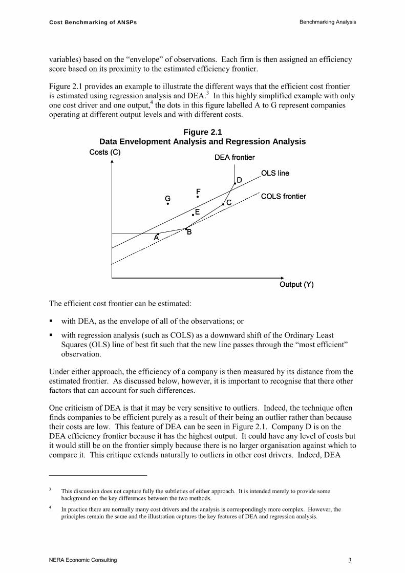
Figure 2.1 provides an example to illustrate the different ways that the efficient cost frontier is estimated using regression analysis and DEA.3 In this highly simplified example with only one cost driver and one output,4 the dots in this figure labelled A to G represent companies operating at different output levels and with different costs.
Figure 2.1 Data Envelopment Analysis and Regression Analysis
Output (Y)
Costs (C)
•
••
•
•
••
OLS line
COLS frontier
DEA frontier
A
F
E
D
C
B
G
Output (Y)
Costs (C)
•
••
•
•
••
OLS line
COLS frontier
DEA frontier
A
F
E
D
C
B
G
The efficient cost frontier can be estimated:
with DEA, as the envelope of all of the observations; or
with regression analysis (such as COLS) as a downward shift of the Ordinary Least Squares (OLS) line of best fit such that the new line passes through the “most efficient” observation.
Under either approach, the efficiency of a company is then measured by its distance from the estimated frontier. As discussed below, however, it is important to recognise that there other factors that can account for such differences.
One criticism of DEA is that it may be very sensitive to outliers. Indeed, the technique often finds companies to be efficient purely as a result of their being an outlier rather than because their costs are low. This feature of DEA can be seen in Figure 2.1. Company D is on the DEA efficiency frontier because it has the highest output. It could have any level of costs but it would still be on the frontier simply because there is no larger organisation against which to compare it. This critique extends naturally to outliers in other cost drivers. Indeed, DEA
3 This discussion does not capture fully the subtleties of either approach. It is intended merely to provide some
background on the key differences between the two methods. 4 In practice there are normally many cost drivers and the analysis is correspondingly more complex. However, the
principles remain the same and the illustration captures the key features of DEA and regression analysis.
Cost Benchmarking of ANSPs Benchmarking Analysis
NERA Economic Consulting 4
tends to characterise many companies as being on the efficient frontier, particularly when there are several cost drivers in the model.
In the present study we adopt the parametric regression analysis approach to cost benchmarking. This approach is not so influenced by outliers. In contrast to DEA, it requires the shape of the frontier to be known, or assumed, in advance. In some cases the choice that is made may be somewhat arbitrary. In the case of air navigation service provision, we aim to set out a formulation for the cost function of ANSPs that is based on our a priori expectations, and estimate the parameters of this cost function using the available data.
A further important criticism of both the DEA and COLS approach to cost benchmarking is the assumption made in each method that the residual, or distance from the frontier, is entirely due to inefficiency. The presence of measurement error in either costs or cost driver data leads to overestimation of inefficiencies. In addition, cost functions do not, in general, capture every factor that influences costs and is outside management control. Some factors are not measurable, while others may apply only to one company and so their effect cannot be distinguished from inefficiency. Where there are omitted variables, the residual in a COLS model may be a biased measure of inefficiency. Likewise in a DEA model, omitted variables or measurement errors can also seriously bias the estimated efficiencies of firms.
In the regression analysis framework, one common method for accounting for the problems of errors in the cost function is SFA. This method separates the model’s residual into two components, a symmetrically distributed term to capture random errors in the cost function, and a bounded-at-zero term to capture inefficiency. The intuition behind this framework is that, since inefficiency must lead to higher costs and never lower costs, it must be bounded from below at zero. Random errors in the cost function, in contrast, may be either positive or negative with equal a priori likelihood.
The empirical analysis in this report uses the SFA method to estimate a cost frontier and individual cost efficiencies. In Section 5, we develop the ideas underlying SFA further in the context of setting out our econometric methodology for the present study.
2.2. Benchmarking in Other Industries
As noted in Section 2.1, benchmarking is now used by some utility regulators to inform their assessments of firms’ current efficiency. Such techniques have been used by regulators in countries including the US, Australia, Ireland, the Netherlands, the UK and in Latin America, and have been applied to a range of different industries and sectors. In broad terms, there are two types of study:
efficiency comparisons within a single country – this is possible where an industry is served by a number of different companies, such as regional water suppliers or electricity distribution companies. The fact that the companies are in the same country, and are often of broadly similar size, may remove some of the external differences that can distort efficiency comparisons (but many remain nevertheless, even within a single country); and
international benchmarking – though more problematic than comparisons within a single country, such studies may nevertheless be attractive for regulators setting a price cap for an industry served by a single national monopolist. Often, however, the use of international comparators introduces additional external factors that are difficult to adjust for fully, eg labour market and geographical variables.

Cost Benchmarking of ANSPs Benchmarking Analysis
NERA Economic Consulting 5
These studies provide meaningful inputs to regulators’ decisions, and therefore can have a potentially significant impact on the prices that regulated firms are allowed to charge. In the worst examples of regulatory practice, the results from benchmarking studies have entered the regulator’s price cap calculations in quite formulaic ways, while in other cases regulators have used the results of benchmarking analysis alongside other efficiency indicators to reach a partly subjective (but more balanced) view of future operating costs.
Mindful of the difficulty of adjusting for external differences between firms, many studies have confined themselves to firms of roughly similar size; but there are exceptions. For example, for a regulatory review in 2000 the Dutch energy regulatory (DTe) commissioned a consultancy study that applied DEA to a sample of 18 electricity distribution companies. Half of the companies in the sample had outputs (across a range of different measures) that were less than five per cent of those of the regulated company, NuonNet. Even though the consultant’s own analysis suggested “unexplained scale effects” (so that higher than predicted costs were observed for large companies), the regulator chose to assume that these represented inefficiency.5
2.3. Benchmarking Air Navigation Service Provision
For a number of years, the PRU has been actively involved in assessing the efficiency of ANSPs in Europe. Since 1999, it has published an annual Performance Review Report, which presents a range of information in relation to four key performance areas: safety, delays, flight-efficiency and cost-effectiveness. The 2005 report presents high level cost indicators, such as the cost per km flown, and contains some qualitative discussion of external factors (such as complexity) that may affect these indicators. But it does not include any statistical analysis to adjust for such factors or otherwise to estimate ANSP efficiency.6
Since 2003, this high level analysis has been supplemented by an annual ATM Cost-Effectiveness (ACE) Benchmarking Report. These reports are based on data supplied by 34 ANSPs in compliance with a mandatory specification for information disclosure, and which have also been subject to extensive validation and analysis. In addition to showing overall unit cost measures, the ACE reports seek to identify the reasons for some of the observed cost differences by breaking down unit costs into three main components, as illustrated in Figure 2.2.
5 We note that this seems to require an extraordinary burden of proof: if companies are assumed to be inefficient simply
because observed (and to some extent systematic) cost differences cannot be explained by the consultant’s model. 6 As noted below, earlier Performance Review Reports did include some results based on regression analysis.

Cost Benchmarking of ANSPs Benchmarking Analysis
NERA Economic Consulting 6
Figure 2.2 PRU Framework for Cost Effectiveness Analysis
Staff costs forATCOs in OPS
Compositeflight-hours
ATCO hourson duty
ATCOs in OPS
ATM/CNSprovision costs
Average hours on duty
Employment costs per ATCO
Support cost ratio
ATCO-hour productivity
Employment costs per ATCO-hour
Financial cost-effectiveness
indicator
The three main components of the PRU’s cost-effectiveness indicators are:
ATCO-hour productivity – defined as the number of flight hours handled by each ATCO hour. This is likely to be influenced by sector productivity (reflecting whether the number of sectors is optimal for the volume and pattern of traffic), staffing per sector and also ATCO productivity (reflecting, for example, the efficiency and flexibility of ATCO rostering). In addition, however, it is important to recognise that a single flight hour can make different demands on ATCOs, depending on the nature of the flight and the extent to which it interacts with other traffic. The likely impact of such differences, which fall within the general idea of “complexity”, is discussed in Section 3.2 below;
ATCO employment costs, which will be partly within management’s control (reflecting the outcome of negotiations over wages and working practices) but will also reflect local economic conditions that are outside of management’s control; and
support costs, and in particular the ratio of total ATM/CNS provision costs to ATCO employment costs.
The ACE reports also contain an analysis of ATCO-hour productivity for individual Area Control Centres (ACCs).7 For this analysis, the PRU groups ACCs into four clusters (including two sub-clusters), each with broadly similar degrees of complexity. But there is no further attempt to quantify the impact of complexity on ATCO productivity, or derive specific efficiency estimates.
7 The sample covers 66 ACCs, as compared with 34 ANSPs. The majority of the ANSPs operate only a single ACC, but
larger countries (such as France, Germany, Italy, Spain and UK) tend to have 4 or 5 ACCs, and the Ukraine has 6.
Cost Benchmarking of ANSPs Benchmarking Analysis
NERA Economic Consulting 7
The PRU did attempt an econometric analysis of EUROCONTROL Member States costs (for en-route services only) in 2000.8 Based on five years of data and 16 States, the PRU estimated an equation that related total en-route costs to the size of airspace controlled, a measure of traffic density, average route length, and the percentage of overflights (as a proxy for traffic complexity) while controlling for the time trend. This work was updated in 2001,9 with an extra year’s data and a slightly larger sample. Average route length was dropped, while refined measures of traffic density and complexity were introduced. But the PRU noted then that further work to better assess the unexplained cost differences would require effective information disclosure by ANSPs on relevant input prices and quantities. Similar results have been included in some subsequent Performance Review Reports, most recently in 2003 with an additional variable included to capture seasonal traffic variability and further refinements to the complexity metrics.
8 See EUROCONTROL (2000). 9 See EUROCONTROL (2001).
Cost Benchmarking of ANSPs Cost Function for Air Navigation Service Provision
NERA Economic Consulting 8
3. Cost Function for Air Navigation Service Provision
3.1. Economic Theory of Costs and Production
The core economic theory underlying the formulation of an industry cost frontier supposes that the minimum costs a producer in that industry can achieve, when using the most efficient technology available, are a function of its output and the prices of its factor inputs.10 The cost function is based on the behaviour of a representative cost-minimising producer who is able to control the amount of each input used subject to producing a given output. These assumptions imply that the cost function must have certain properties, namely: linear homogeneity and concavity in input prices; and, monotonicity in input prices and output. Linear homogeneity in input prices means that if all input prices double, then costs must also double. Concavity in input prices means that if one input price doubles then costs must not more than double. Monotonicity in input prices and output means that costs must never fall when either input prices or outputs rise. These properties place theoretical restrictions on the empirical estimation.11
The existence of economies or diseconomies of scale in the industry can be inferred from the cost function. This is done by examining the impact on unit costs when output increases. In the context of network industries, however, a variable capturing the size of the network is generally added to the cost function. This allows redefining the analysis of economies of scale in network industries to distinguish economies of scale from economies of density.
Economies of scale are defined in relation to the impact on unit costs when both output and size of network increase in the same proportion and other characteristics of the operating environment are held constant. There are economies of scale when unit costs fall as output and network size increase, and there are diseconomies of scale when unit costs rise as output and network size increase.
Economies of density are defined in relation to the impact on unit costs when output increases holding network size constant. There are economies of density when unit costs fall as output increases on a fixed network and there are diseconomies of density when unit costs rise as output increases on a fixed network.
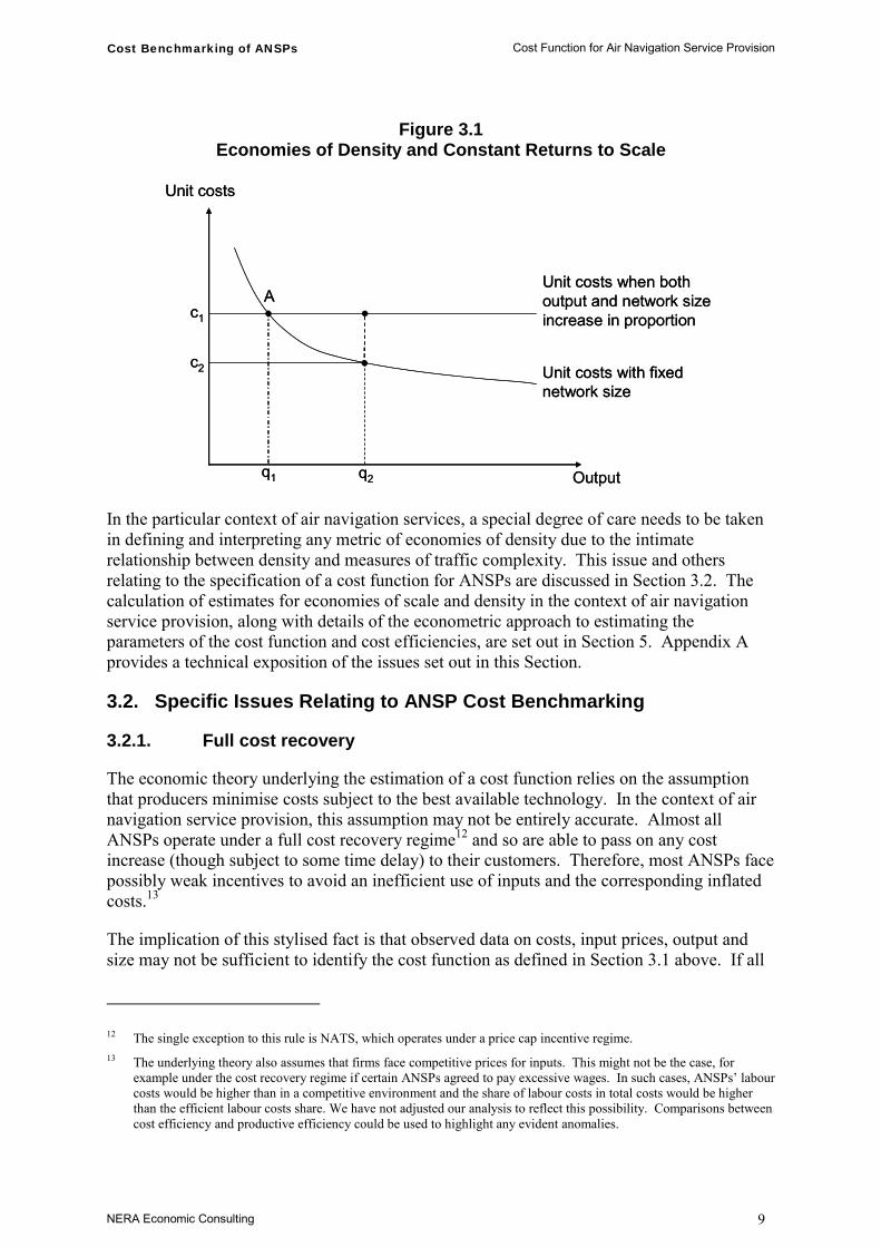
Figure 3.1 illustrates the distinction between economies of scale and economies of density by showing a case where there are economies of density but constant returns to scale. Point A shows unit costs, c1, at the existing output level, q1. If output were to increase on the fixed network from q1 to q2, then unit costs would fall to c2 along the curve which shows unit costs with the network fixed. However, if an increase in output from q1 to q2 is accompanied by an equi-proportionate increase in the network size, then unit costs would not change as the ANSP would move out along the horizontal unit cost line that shows constant returns to scale.
10 The cost function captures the same technology as the production function, which in turn describes the relationship
between factor inputs and the maximum output producers could achieve. The relationship between costs and production is therefore referred to as a “dual” relationship. See Chambers (1988) for a detailed technical exposition of the dual approach to economic cost and production analysis.
11 The restrictions are discussed in Section 5.
Cost Benchmarking of ANSPs Cost Function for Air Navigation Service Provision
NERA Economic Consulting 9
Figure 3.1 Economies of Density and Constant Returns to Scale
Output
Unit costs
Unit costs with fixed network size
Unit costs when both output and network size increase in proportion
A
q1 q2
c1
c2
Output
Unit costs
Unit costs with fixed network size
Unit costs when both output and network size increase in proportion
A
q1 q2
c1
c2
In the particular context of air navigation services, a special degree of care needs to be taken in defining and interpreting any metric of economies of density due to the intimate relationship between density and measures of traffic complexity. This issue and others relating to the specification of a cost function for ANSPs are discussed in Section 3.2. The calculation of estimates for economies of scale and density in the context of air navigation service provision, along with details of the econometric approach to estimating the parameters of the cost function and cost efficiencies, are set out in Section 5. Appendix A provides a technical exposition of the issues set out in this Section.
3.2. Specific Issues Relating to ANSP Cost Benchmarking
3.2.1. Full cost recovery
The economic theory underlying the estimation of a cost function relies on the assumption that producers minimise costs subject to the best available technology. In the context of air navigation service provision, this assumption may not be entirely accurate. Almost all ANSPs operate under a full cost recovery regime12 and so are able to pass on any cost increase (though subject to some time delay) to their customers. Therefore, most ANSPs face possibly weak incentives to avoid an inefficient use of inputs and the corresponding inflated costs.13
The implication of this stylised fact is that observed data on costs, input prices, output and size may not be sufficient to identify the cost function as defined in Section 3.1 above. If all
12 The single exception to this rule is NATS, which operates under a price cap incentive regime. 13 The underlying theory also assumes that firms face competitive prices for inputs. This might not be the case, for
example under the cost recovery regime if certain ANSPs agreed to pay excessive wages. In such cases, ANSPs’ labour costs would be higher than in a competitive environment and the share of labour costs in total costs would be higher than the efficient labour costs share. We have not adjusted our analysis to reflect this possibility. Comparisons between cost efficiency and productive efficiency could be used to highlight any evident anomalies.
Cost Benchmarking of ANSPs Cost Function for Air Navigation Service Provision
NERA Economic Consulting 10
ANSPs are operating inefficiently then, without further knowledge of the minimum inefficiency, the true frontier will be hidden from observation.
The inability to estimate the true cost frontier does not affect the ability to provide a meaningful benchmarking of ANSPs’ relative efficiency levels. However, it does bias measures of absolute inefficiencies and any corresponding assessment of the potential for cost savings.
In our empirical analysis, we estimate a cost function using ANSP data. The results we present on the parameters of the cost frontier and the cost inefficiencies are therefore contingent on the corporate governance frameworks that actually exist rather than for an idealised cost-minimising ANSP. It will be important to interpret the results with this in mind.
3.2.2. Economies of scale and density
ANSP costs are likely to vary with both the size of airspace controlled and the volume of traffic using the airspace. The size of airspace controlled will affect the physical infrastructure required, for example to communicate with aircraft and to monitor their progress (by means of radar surveillance). We would expect this to affect mainly capital costs.
The volume of traffic is then likely to have a more direct impact on both capital and labour costs. First it will influence the number of Air Traffic Control Officers (ATCOs) and associated workstations that are required.14 In turn, these will have a major impact on each ANSP’s support costs.
A key constraint, which drives much of the relationship between output and costs, is the volume of traffic that can be safely controlled by a single ATCO crew with a single workstation. Once a particular sector cannot safely handle any more traffic, an ANSP must either open a new sector or else it must reconfigure its existing airspace so that it is divided up into more sectors.15 Both of these will increase the number of ATCOs and workstations required.
But the relationship between traffic volumes and the number of ATCOs and workstations required is not necessarily a straightforward one. Especially at low levels of traffic, an ANSP’s ATCOs and workstations may be poorly utilised, with plenty of capacity to accommodate additional traffic without any significant impact on costs. Strictly, this represents a potential economy of density rather than an economy of scale, as it relates to an increase in output while the network size remains unchanged.
14 In contrast, we observe that the number of ATCOs and workstations will not necessarily be closely related to the
physical volume of airspace controlled. Considering, for example, an ANSP that deals with a single flight a day (leaving aside questions of whether ATC would actually be required in this situation!). Provided that flight comes and goes within a single, predictable shift, then only one ATCO and workstation might be required, no matter how large or small the physical airspace controlled by that ANSP.
15 This might involve simply splitting a single sector into two separate sectors, or occasionally it might involve a large scale “resectorisation” exercise.

Cost Benchmarking of ANSPs Cost Function for Air Navigation Service Provision
NERA Economic Consulting 11
The potential for economies of density may weaken, however, at the point where additional traffic requires new sectors to be opened. Indeed, marginal productivity is likely to decrease as the number of sectors increases because the combined capacity of two separate sectors will often be a little less than twice the capacity of a single sector. Lower sector marginal productivity, however, does not necessarily imply overall diseconomies of density, given the important role of other cost components, eg support costs.
More importantly, the requirement for ATCOs and workstations will also depend on the complexity of traffic, and this may well change as the volume of traffic accommodated within a fixed network increases. The demands placed on an ATCO in relation to a single flight hour will depend on how “difficult” it is to control a particular flight. If, within a particular sector, there are many planes flying in different directions (both horizontally and also vertically, for example because some are taking off from or landing at a nearby airport) and at different speeds, then this traffic will place more demands on an ATCO than an equivalent number of planes following each other along a single route at the same speed.
3.2.3. Basic efficiency measurement concepts
This study aims to examine the relative cost inefficiencies among ANSPs by estimating a cost function. This approach should capture two separate components of economic inefficiency:
• productive (or technical) inefficiency – when a firm uses larger amounts of inputs to produce the same level of output as an efficient comparable firm; and
• allocative inefficiency – when a firm uses a suboptimal mix of inputs given the respective input prices.
Many of the possible sources of inefficiency for ANSPs are likely to fall within the first category – productive inefficiency. This is because there are few opportunities for ANSPs to switch resources, for example to use more capital and fewer labour inputs. Productive inefficiency appears to be more likely, for example because some ANSPs have inflexible rostering of ATCOs or high corporate overheads. Therefore, our a priori expectation is that allocative inefficiency will be small relative to productive inefficiency. Nevertheless, both concepts of inefficiency are captured by the cost benchmarking approach used for this project.
One possible alternative approach would be to estimate a production function rather than a cost function. This would focus purely on productive (or technical) inefficiency, by examining either the maximum potential output given a set of inputs, or the minimum set of inputs that can produce a given output.16 This approach might be appropriate, as we expect most inefficiency to be productive rather than allocative. But it would require data on physical capital inputs, rather than prices.17
16 Schmit and Knox Lovell (1979) provide a good exposition of both forms of SFA. 17 In theory, by carrying out production benchmarking as well as cost benchmarking, we could examine both total
inefficiency and the division of this between allocative and productive inefficiency. But this assumes that both approaches can be implemented in a way that produces robust and reliable estimates of inefficiencies. As explained in Section 6.3, we believe that our preferred cost function overestimates inefficiency

Cost Benchmarking of ANSPs Cost Function for Air Navigation Service Provision
NERA Economic Consulting 12
3.2.4. Total cost and variable cost functions
The cost function described in Section 3.1 is based on the assumption that the quantities of all inputs are freely variable and under the control of ANSP managers. In the long run this is true by definition. However, in any individual year this assumption can be invalid. ANSPs develop their capacity to meet expected demand by ensuring there are sufficient ATCOs and workstations available, a process that often involves discrete changes such as the introduction of new systems, resectorisation, or other changes to the use of airspace. Unanticipated changes in the growth of traffic volumes might be accommodated by either accelerating or decelerating planned recruitment, training and investments. However, in the case of an actual fall (rather than just slower than expected growth) in traffic volumes, especially if demand is expected to bounce back relatively quickly, it may not be practical or sensible for ANSPs to cut back on capacity in order to save costs. In such cases an ANSP may operate with excess capacity in the short run.
The implication of the failure to satisfy the assumption of full immediate control over all inputs is that an ANSP may be assigned a low efficiency score – not because it has operated inefficiently, but because demand has been lower than expected. If demand is different from expected, an ideal model should not assign an ANSP a low efficiency score as a result. In theory, an efficient ANSP would determine the rate of capital formation (investment) by considering the expected levels, types and patterns of traffic and making the trade-off between the costs of bearing surplus capacity on the one hand and the costs of capacity shortfalls on the other. A capacity shortage results in a greater risk of causing delays to flights and is hence not straightforwardly captured in monetary terms.18
One potential solution to the problem of input fixity and the inability to adjust the input mix in order to accommodate changes in output is to focus attention on variable costs only, and to model explicitly a set of flexible inputs and a set of fixed or quasi-fixed inputs that cannot be rapidly adjusted to reflect changing conditions.19 Often in the variable cost function capital is assumed to be the quasi-fixed input. Therefore variable costs are modelled as a function of the quantity of capital, the price of variable inputs, output, network size and other exogenous factors. If capital and labour are complements,20 a variable cost model predicts that an ANSP with surplus capital will have higher variable costs than a similar ANSP with no surplus capacity.
Despite the possible advantages of the variable cost model in its ability to separate the effects of demand shocks from inefficiency,21 the inefficiency estimates from this model will, by construction, only relate to variable cost efficiency. In effect, the total cost model aggregates
18 Section 3.2.5 discusses the issue of how to account for delays in the context of the quality of service provided. 19 The use of a variable cost model is also sometimes justified because of problems measuring capital costs. In our case,
however, any measurement errors would be likely to affect both approaches since the total cost model requires a measure of capital input prices, while the variable cost model requires a measure of capital stock.
20 We would expect, a priori, that capital and labour would be complements, rather than substitutes, for ANSPs. There would appear to be few opportunities to substitute more machines for fewer people in air navigation service provision. The converse is more likely, that when there are more machines, more labour is likely to be needed to operate and maintain them.
21 Such advantages might be limited, moreover, because some labour costs are also likely to be fixed or quasi-fixed. This reflects both the transactions costs associated with hiring and firing labour and also the sunk costs that have been incurred in the training of ATCOs and other specialists.

Cost Benchmarking of ANSPs Cost Function for Air Navigation Service Provision
NERA Economic Consulting 13
three measures of efficiency. It covers the costs of providing capacity; the costs of operating the capacity; and the amount of capacity provided. Whilst from year to year companies may be assigned efficiency scores at odds with reality due to demand shocks, for a long term perspective on efficiency it is useful for completeness to have all these three measures embedded in the metric of cost efficiency.
The results reported in this paper relate to a total cost model. In order to mitigate the issues related to input fixity, our estimates of cost inefficiencies are based on averages over the four year sample period. Inefficiency is likely to change from year to year; however there is limited scope to distinguish these effects from uncontrollable demand shock effects. By estimating average inefficiency, the impact of year to year demand shocks on the inefficiency measures is diluted and so the measure is a better representation of inefficiency. Empirically the distinction between total cost inefficiency and variable cost inefficiency for this sample of ANSPs does not seem of paramount importance. Our analysis of the impact of each approach (not shown in this report) shows that in this application total cost and variable cost functions produce very similar efficiency rankings.
3.2.5. Quality of service
The key measure of quality of service for ANSPs is the prevalence of delays. As discussed in Section 3.2.3, one might expect delays to be correlated with the underprovision of capacity. If some ANSPs operate at a lower spare capacity level on average we should observe that they are more severely affected by delays than other ANSPs. Operating closer to full capacity should be associated with lower costs than providing the same output with significant spare capacity still available. Thus, a priori we might expect a negative relationship between costs and delays.
The above argument suggests that controlling for delays in the cost function would be needed to ensure fair comparisons across ANSPs in respect of quality of service. However, there are reasons to believe that a negative correlation between delays and costs may now be less likely to emerge empirically. In recent times, (ground) ATFM delays have fallen and in many cases they are now very low indeed. Compared with several years ago, one-off or random events are more likely to account for a greater (and possibly quite large) proportion of observed ATFM delays than a general underprovision of capacity. Such events might include one-off systems failures, problems caused by industrial action (including in other countries), or the impact of new investment (such as opening of a new control centre or the introduction of new systems, which may operate at reduced capacity for a short period of time). Furthermore, delays can only capture insufficient capacity; they cannot be used to proxy for the existence of spare capacity (ie there are no “negative” delays) and this truncation of delays at zero is bound to weaken the negative correlation between costs and delays described above. Our approach is therefore to make no adjustment for quality of service and so to implicitly assume that service quality is not a significant cost driver.22
22 This approach is backed up by preliminary estimation results that found no evidence of an impact of observed delays on
costs.

Cost Benchmarking of ANSPs Cost Function for Air Navigation Service Provision
NERA Economic Consulting 14
3.2.6. Other cost drivers
ANSP costs are likely to be dependent on the characteristics of the airspace controlled. These can be grouped under the banner of airspace “complexity”. Complexity is quite difficult to define in general terms. In part, this is because there are a number of different aspects of flight patterns that can add to ATCOs’ workload. As the critical task for air traffic control is to maintain a safe separation between planes at all times, “complexity” covers anything that increases the likelihood that planes will potentially interact with each other (and therefore ATCOs may need to take action to ensure that safe distances are maintained). In addition to the sheer volume of aircraft in a particular area, complexity may be affected by:
the horizontal routes of aircraft, for example whether certain routes cross each other and therefore give rise to potential conflict situations;
the vertical evolution of aircraft, and whether there is a mix of traffic that may be either climbing, descending or cruising within a particular area of airspace; and
the mix of traffic speeds. Even if all planes are following the same route and flying in the same direction, if some are faster than others then ATCOs will need to ensure that faster planes do not catch up with preceding slower planes.
All of these factors affect the volume of aircraft that a single team of ATCOs can deal with at any one time. An ANSP with a “complex” pattern of traffic will therefore need more ATCOs (and thus more workstations, and potentially more non-ATCO staff, and so on) as compared with another ANSP that handles the same total volume of traffic but with a lower level of complexity.
In addition, since ANSPs must be able to provide sufficient ATCOs and workstations to cope with peak demand, the peakiness of traffic over time will also affect the relationship between output and costs. If traffic varies in a predictable manner between certain times of the day or certain days of the week, then it may be possible for ANSPs to deal with this peakiness, to some extent at least, by organising ATCO shift patterns so that more cover is always available at these particular times. It is much more difficult for ANSPs to deal with seasonal variations in traffic levels, as they need to employ ATCOs (and indeed other staff) all year round rather than on a seasonal basis. They will therefore need a greater number of ATCOs to handle a certain annual volume of traffic, as compared with an ANSP whose traffic is spread evenly throughout the year.
Cost Benchmarking of ANSPs Data Used for the Analysis
NERA Economic Consulting 15
4. Data Used for the Analysis
The main data used in our empirical analysis have been drawn from information provided by ANSPs in their mandatory annual returns to EUROCONTROL’s Performance Review Unit (PRU). The data used in this study relate to civil ATM/CNS provision only and for gate-to-gate, ie en-route plus terminal air navigation services. The data exclude costs associated with ATM services provided to military operational air traffic (OAT), Oceanic ANS, Aeronautical Meteorological (MET) services and airport management operations. ATM/CNS provision costs account for approximately 88 per cent of total costs and are, broadly speaking, under the direct control and responsibility of the ANSP.23 Other expenses, including payments to governmental (regulatory) authorities, non-recoverable VAT, and EUROCONTROL costs, are predominantly outside the control of ANSP management. These costs are therefore not included in the analysis.
The ANSPs in the sample vary substantially in terms of the size of the airspace controlled, the volume and characteristics of traffic controlled and their organisational governance structure. Notwithstanding this heterogeneity, the annual returns record sufficient information, on a broadly comparable basis, to allow for a fair and robust comparative cost effectiveness analysis of ANSPs.
The dataset contains annual data for 34 European ANSPs for 2001 to 2004 and includes information at the level of the ANSP on costs, inputs, outputs, traffic variability and complexity characteristics. To supplement these data, cost-of-living indices were also added from the International Monetary Fund, World Economic Outlook Database, April 2006.
The EUROCONTROL data have been subjected to an extensive validation process by the ACE Working Group, which includes ANSP representatives and airspace users in addition to the PRU. While the annual information disclosed to the PRU is generally comparable across ANSPs, there remain some irregularities between ANSPs in terms of certain accounting treatments.
A detailed description and analysis of the EUROCONTROL data, including all the data validation checks undertaken by the PRU, can be found in the ACE benchmarking reports, EUROCONTROL (2003b, 2004, 2005a, 2006). The remainder of this section discusses specific aspects of the data relating to the main categories: costs, inputs and input prices, outputs, network size and traffic characteristics. It then reports descriptive statistics and presents graphs of key correlations between variables.
4.1. Costs
The dependent variable in our empirical analysis is gate-to-gate ATM/CNS provision costs for each ANSP. Costs are measured in constant 2004 Euros for the sample.
23 This figure of 88 per cent was drawn from EUROCONTROL (2006), p.13.

Cost Benchmarking of ANSPs Data Used for the Analysis
NERA Economic Consulting 16
The available data on costs are unbalanced. For some ANSPs, data were missing for a given year. In addition, due to problems with the data, we have excluded from the sample all observations for HCAA Greece, and DCAC Cyprus data for 2002 and 2003.24
The final sample therefore contains 33 ANSPs and 125 observations in total.
Detailed descriptions and non-econometric examinations of the ANSP cost data are contained within EUROCONTROL (2003b, 2004, 2005a and 2006). Table 4.1 provides a high-level summary of the information on the breakdown of costs for the 34 ANSPs in our sample in 2004.
Table 4.1 shows that staff costs are the largest proportion of total ATM/CNS costs, with 59.7 per cent on average for the ANSPs in 2004. Direct operating costs are the second highest contributor to total cost at 18.8 per cent on average. Depreciation and cost of capital are smaller components on average, though they account for a higher proportion of costs for some individual ANSPs (for example, depreciation accounted for 30.2 per cent of FYROM CAA’s total costs in 2004).
Table 4.1 Gate-to-gate ATM/CNS Provision Costs, 2004
Cost Category Weighted average
Standard deviation Minimum Maximum
ATM/CNS Provision costs (€'000) 571,198 270,572 2,792 955,646 Staff costs (%) 59.7% 13.0% 24.4% 75.2% Direct (non-staff) operating costs (%) 18.8% 7.5% 12.0% 41.3% Depreciation costs (%) 14.6% 5.2% 5.9% 30.2% Costs of capital (%) 6.1% 6.7% 1.6% 24.9% Exceptional items (%) 0.8% 1.5% 0.0% 8.4% Source: NERA. Note: Based on 33 observations. Weighted average is weighted by total costs. Standard deviation, minimum and maximum values are calculated using unweighted observations.
Depreciation costs are notoriously difficult to measure on an objective basis because they typically need to be estimated, rather than simply recorded. When technological progress leads to changing asset lifetimes and prices over time, the choice of depreciation policy may entail a substantial degree of discretionary judgement. Asset lives and depreciation profiles need to be estimated, which can lead to a difference between economic and accounting depreciation, and a difference between firms that use different policies. Although there are guidelines such as the EUROCONTROL document “Principles for Establishing the Cost-Base for Route Facility Charges and the Calculation of the Unit Rates”, there may be inconsistencies in the treatments given to assumed asset lives, depreciation profiles and capitalisation policy.
The cost of capital is reported by each ANSP and there are issues of consistency (since some ANSPs report the economic cost of capital and others report only the financial cost) as well as problems of comparability across ANSPs. The reported costs of capital ranged from 2.5 per cent for ENAV to 16 per cent for MoldATSA in 2004.25 The asset bases to which these rates are applied also vary. In most cases the Net Book Value of fixed assets is used (which 24 This was done in agreement with EUROCONTROL and was due to potential problems with the data. 25 See EUROCONTROL (2006), Table 3.5.
Cost Benchmarking of ANSPs Data Used for the Analysis
NERA Economic Consulting 17
will also be affected by differences in depreciation policies, as noted above), but for some ANSPs working capital is also included in the asset base.
For these reasons there may well be measurement errors in the data on depreciation and cost of capital and, as such, the results on efficiencies are subject to this caveat.
4.2. Outputs
Within the category of ATM/CNS, the principal services provided by ANSPs comprise en-route and terminal control services. Due to definitional differences across ANSPs and how costs are allocated between the two categories of service, it is appropriate to focus on a combined measure of output. Moreover, there are significant empirical advantages to restricting attention to a single combined measure of “gate-to-gate” output, particularly when, as in the present case, the dataset available is small and the two output measures are highly correlated.
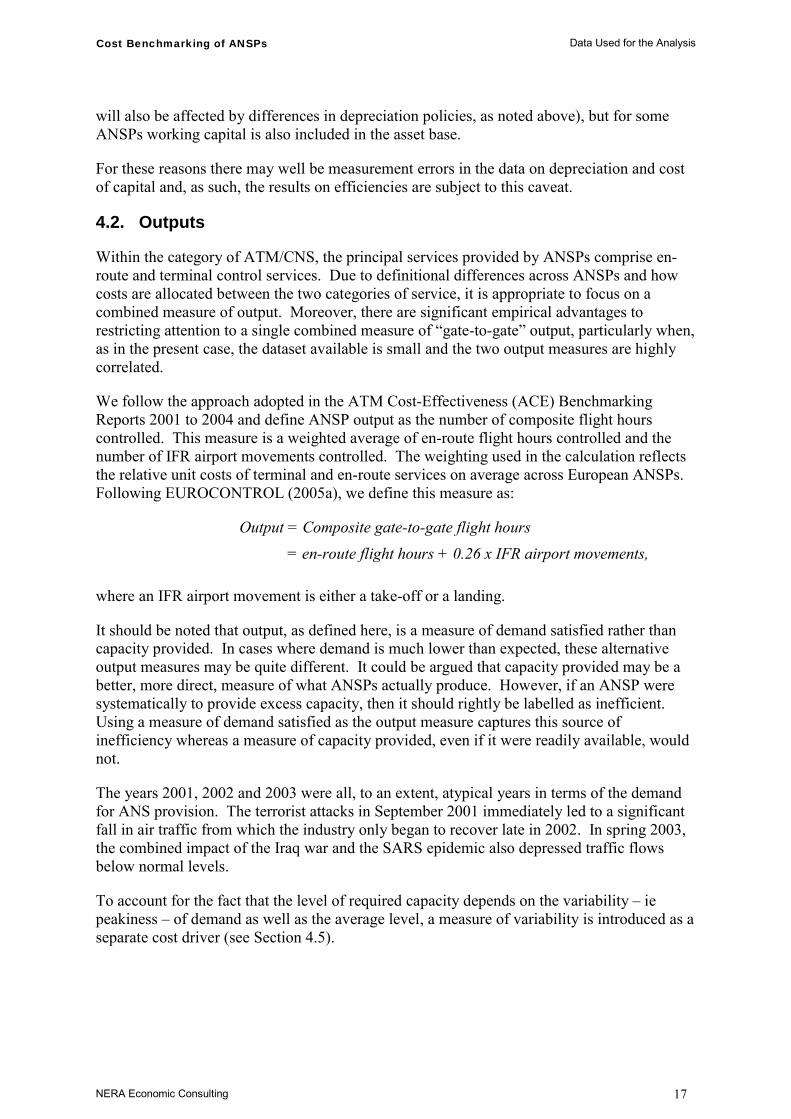
We follow the approach adopted in the ATM Cost-Effectiveness (ACE) Benchmarking Reports 2001 to 2004 and define ANSP output as the number of composite flight hours controlled. This measure is a weighted average of en-route flight hours controlled and the number of IFR airport movements controlled. The weighting used in the calculation reflects the relative unit costs of terminal and en-route services on average across European ANSPs. Following EUROCONTROL (2005a), we define this measure as:
Output = Composite gate-to-gate flight hours
= en-route flight hours + 0.26 x IFR airport movements,
where an IFR airport movement is either a take-off or a landing.
It should be noted that output, as defined here, is a measure of demand satisfied rather than capacity provided. In cases where demand is much lower than expected, these alternative output measures may be quite different. It could be argued that capacity provided may be a better, more direct, measure of what ANSPs actually produce. However, if an ANSP were systematically to provide excess capacity, then it should rightly be labelled as inefficient. Using a measure of demand satisfied as the output measure captures this source of inefficiency whereas a measure of capacity provided, even if it were readily available, would not.
The years 2001, 2002 and 2003 were all, to an extent, atypical years in terms of the demand for ANS provision. The terrorist attacks in September 2001 immediately led to a significant fall in air traffic from which the industry only began to recover late in 2002. In spring 2003, the combined impact of the Iraq war and the SARS epidemic also depressed traffic flows below normal levels.
To account for the fact that the level of required capacity depends on the variability – ie peakiness – of demand as well as the average level, a measure of variability is introduced as a separate cost driver (see Section 4.5).
Cost Benchmarking of ANSPs Data Used for the Analysis
NERA Economic Consulting 18
4.3. Input Prices
Air navigation service provision requires both labour and capital inputs. In addition, there is a third broad category of input, direct operating costs, which includes miscellaneous items such as energy, materials, etc. In this section, we describe each of the input categories, how their prices have been calculated, and the data issues therein that affect our analysis.
4.3.1. Labour input prices
There are two distinct categories of labour employed by ANSPs: Air Traffic Control Officers in Operations (ATCOs in OPS), which accounts for 46 per cent of employment costs on average; and non-ATCO staff, which accounts for the remaining 54 per cent.26 Input prices for each of these classes of labour have been calculated by dividing employment costs for the class by, in the case of ATCOs in OPS, hours worked, and in the case of non-ATCO staff, the number of FTE employees. Employment costs per hour are a preferred measure of labour input prices since employment costs per FTE reflect both the cost of labour and the number of hours worked. Unfortunately, no hourly employment cost data are available for non-ATCO staff. ATM/CNS provision is relatively labour intensive, with the average cost share of labour equal to 60 per cent of total costs.27
4.3.2. Capital input prices
Capital inputs used in ATM/CNS provision are varied. They include buildings, controller working positions, various ATM equipment (with sophisticated flight and radar data processing systems) and CNS infrastructure (such as surveillance radar).
The appropriate input price to use for capital inputs is the rental rate, which is the unit rate that covers the user cost of the input, ie depreciation plus the cost of capital. This is likely to vary over time and between ANSPs due to changes in interest rates and capital equipment prices. It is also likely to change over time due to the lumpy nature of capital investment, which leads to a variable stream of depreciation and capital costs.
When an ANSP has recently undertaken a significant investment, such as implementing a new ATC system, then the value of fixed assets in the business will be higher than when the majority of its assets have a low remaining economic life. The user cost of capital will thus also be higher. For large ANSPs, it may be possible to maintain a reasonably steady capital investment programme such that new investment is roughly equal to depreciation year on year. For smaller ANSPs this is unlikely. EUROCONTROL (2005a) documents capital expenditure to depreciation ratios for all ANSPs in 2003 and finds a wide variation. Ratios vary from 0.3 for EANS and MATS, to 9.0 for NATA Albania.28
ANSPs certainly need to replace capital assets when they reach the end of their economic lives. However, the increased capital costs may not be directly offset by falling operating costs, and certainly not by increased output. There may be fewer delays, but otherwise no other immediate or tangible benefits. The implication of this is that in a cost benchmarking
26 These figures were drawn from EUROCONTROL (2006), Figure 2.4, p.14. 27 See EUROCONTROL (2006), Figure 2.4, p.14. 28 See EUROCONTROL (2005a), p.82.
Cost Benchmarking of ANSPs Data Used for the Analysis
NERA Economic Consulting 19
exercise, ANSPs that have recently undertaken substantial capital investment may be treated as inefficient unless some account is taken of the cyclical pattern of capital costs.
To capture variations in the rental rate of capital, over time and across ANSPs, our approach is to specify a physical unit of capital and divide the sum of ANSPs’ annual depreciation and interest cost of capital by their quantity of these capital units. This is a commonly used approach for capturing capital input prices (see, for example, Farsi, Filippini and Greene (2005), who use the number of train seats as a proxy for the physical capital stock of railway companies).
In order to calculate capital input prices for ANSPs, we have used a weighted average of the number of open ACC sector-hours and of Instrument Landing Systems (ILS) localisers as a means of approximating the composition of capital physical inputs for en-route and terminal ANS.
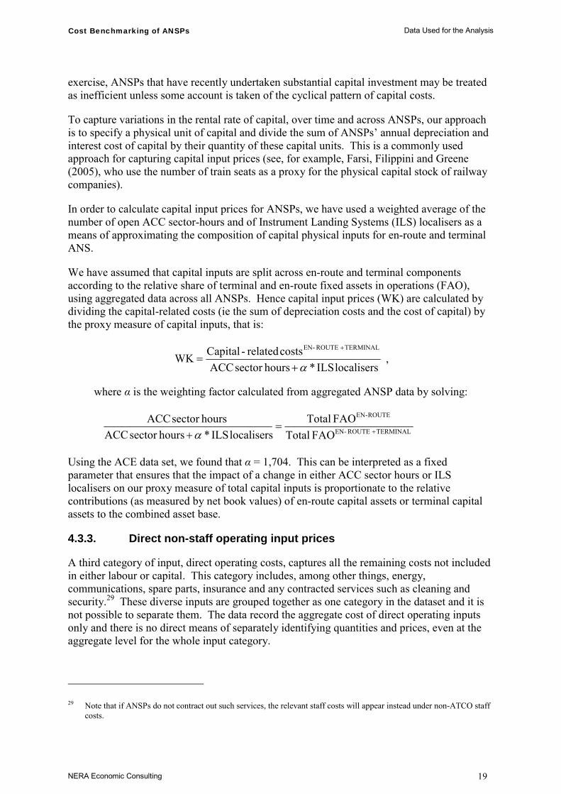
We have assumed that capital inputs are split across en-route and terminal components according to the relative share of terminal and en-route fixed assets in operations (FAO), using aggregated data across all ANSPs. Hence capital input prices (WK) are calculated by dividing the capital-related costs (ie the sum of depreciation costs and the cost of capital) by the proxy measure of capital inputs, that is:
localisersILS*hourssector ACC
costs related-CapitalWKTERMINAL ROUTE -EN
α+=
+
,
where α is the weighting factor calculated from aggregated ANSP data by solving:
TERMINAL ROUTE -EN
ROUTE-EN
FAO TotalFAO Total
localisers ILS* hourssector ACC hourssector ACC
+=+α
Using the ACE data set, we found that α = 1,704. This can be interpreted as a fixed parameter that ensures that the impact of a change in either ACC sector hours or ILS localisers on our proxy measure of total capital inputs is proportionate to the relative contributions (as measured by net book values) of en-route capital assets or terminal capital assets to the combined asset base.
4.3.3. Direct non-staff operating input prices
A third category of input, direct operating costs, captures all the remaining costs not included in either labour or capital. This category includes, among other things, energy, communications, spare parts, insurance and any contracted services such as cleaning and security.29 These diverse inputs are grouped together as one category in the dataset and it is not possible to separate them. The data record the aggregate cost of direct operating inputs only and there is no direct means of separately identifying quantities and prices, even at the aggregate level for the whole input category.
29 Note that if ANSPs do not contract out such services, the relevant staff costs will appear instead under non-ATCO staff
costs.
Cost Benchmarking of ANSPs Data Used for the Analysis
NERA Economic Consulting 20
Given the current lack of precise information on the components of the direct operating input category and the respective cost-shares, the choice of a price index for this input category is fairly arbitrary. The components of direct operating costs are likely to include expenditure incurred at local prices, such as contracted services, utilities and consulting services. We therefore constructed a price index that reflects the cost of living in each country using IMF data (specifically, by comparing GDP measured at current prices and GDP adjusted for purchasing power parity).30
To improve the robustness of cost benchmarking in future, we would recommend that sufficient information is collected to allow a more robust index to be constructed for direct operating inputs. This might involve, for example, a weighted average of industry specific price indices (eg from the energy sector or from specialised manufacturing industries).
In addition, some expenditure falling within this category (perhaps including some materials and specialist consulting services for example) may be incurred at international prices. To take account of this, a weighted average could be used where the weight attached to the domestic cost of living index (or alternative indices) is less than 100 per cent. We have not adopted this approach, as we do not have information about the importance of such costs though we would expect them to be relatively small. If they are significant, however, then a weighted average index would be appropriate.31
4.4. Network Size
In the ACE data set, several metrics can characterise network size:
the average flight transit time, which is obtained by dividing the number of flight-hours by the number of flights within a given airspace;
the size of controlled airspace (in km²) in which the ANSPs are responsible for providing ATC services; and
the volume of the airspace in which the ANSPs are responsible for providing ATC services.
We have used the size of controlled airspace in the analysis. This measure has the advantage of being exogenous and – unlike average transit time – it is not related to our output measure (composite flight-hours controlled). The size of airspace controlled and the volume of controlled airspace are strongly correlated (correlation coefficient of 0.99, which indicates nearly perfect correlation). It should be noted that all three of the possible measures of network size change little over time.
When we calculate economies of density, we will be referring to the elasticity of cost with respect to changes in composite flight-hours holding the size of controlled airspace constant.
30 The cost-of-living index was drawn from the International Monetary Fund, World Economic Outlook Database, April
2006. 31 This approach, with a 50 per cent weight assigned to the domestic cost index, was used in EUROCONTROL (2005b).
Cost Benchmarking of ANSPs Data Used for the Analysis
NERA Economic Consulting 21
4.5. Traffic Characteristics
Other key traffic characteristics driving costs for ANSPs are traffic variability and traffic complexity. Our measure of the temporal variability of air traffic controlled is the ratio of peak week to average week traffic. This variable captures the impact on costs arising where demand is very peaky due to the need for greater capacity, relative to cases where the annual demand profile is flatter.
Traffic complexity is a widely used term in relation to air traffic management yet there is no single measure that perfectly captures it. The ACE Working Group on complexity has defined a set of high level traffic complexity indicators to be used for benchmarking purposes (rather than for operational purposes). The Group concluded that the issues can be combined into two main groups under the heading “traffic complexity”:
“adjusted density” – this gives an indication of the intensity of interactions that a flight in a given airspace would face. The more interactions there are, the denser is the traffic; and
“structural complexity” – this indicator describes the degree to which the interactions during a flight involve differences in vertical orientation (the traffic contains more ascending and descending routes), horizontal orientation (the traffic contains more crossing routes) and speed difference (the traffic contains flights with different speeds).32
A key advantage of these two metrics is that they are independent. Traffic in an area can be dense, but structurally simple; equally, traffic can be structurally complex but sparse. Furthermore, the two impacts are multiplicative – the overall traffic complexity score is computed as the product of the structural complexity and the adjusted density measures.
32 See EUROCONTROL (2005c) for a detailed presentation of the complexity indicators.
Cost Benchmarking of ANSPs Data Used for the Analysis
NERA Economic Consulting 22
4.6. Descriptive Statistics
In this section we present descriptive statistics and graphical analysis of the variables in the dataset described above. Table 4.2 presents descriptive information for the variables in the dataset.
Table 4.2 Descriptive Statistics, 2001 to 2004
Variable name Description (units) Mean Std. Dev. Ratio of Mean to S.Dev.
TC Total costs (€million) 186.0 267.0 0.70
UC Unit costs (€/Y) 306.2 105.8 2.89
WL1 ATCO labour price (€/hour) 54.0 34.5 1.57
WL2 Non-ATCO labour price (€/year) 50,408.0 35,580.4 1.42
WDOC Direct operating cost price (index) 87.4 17.1 5.12
WK Capital input price (index) 267.1 150.9 1.77
Y Composite output (per year) 508,267.5 634,004.7 0.80
N Airspace size (sq. km) 371,494.1 467,781.4 0.79
ZVAR Variability (index) 1.24 0.13 9.24
ZAD Adjusted density (index) 0.09 0.05 1.82
CPX Structural complexity (index) 0.77 0.26 2.98
CSCORE Complexity score (index) 0.07 0.06 1.21
Source: NERA. Note: Based on 125 observations.
4.6.1. Correlation between variables
In this Section, we present a range of graphs plotting pairs of variables to investigate correlations and outliers. A correlation matrix is shown in Table 4.3, and is referred to throughout this section in the graphs and discussion.
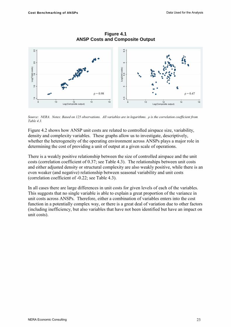
Figure 4.1 presents two scatter graphs. The left-hand side graph plots total costs against the composite output metric (both in logarithmic form) for each ANSP and for each year the data are available. This graph shows that there is an approximately linear relationship between log output and log total costs. The correlation coefficient is 0.98 (see Table 4.3). This graph illustrates wide differences in the composite output metric. At one extreme, there is a cluster of five larger ANSPs (Aena, DFS, DSNA, ENAV and NATS) and at the other extreme there is one very small ANSP (MoldATSA).
The right-hand side graph in Figure 4.1 plots the log of unit costs against the log of composite output. There seems to be only a weak positive relationship between the two variables, characterised by the correlation coefficient of 0.47 (see Table 4.3). Very different levels of unit costs are associated with a given output level.
Cost Benchmarking of ANSPs Data Used for the Analysis
NERA Economic Consulting 23
Figure 4.1 ANSP Costs and Composite Output
1416
1820
22Lo
g(To
tal c
osts
)
8 10 12 14 16Log(Composite output)
4.5
55.
56
6.5
Log(
Uni
t cos
ts)
8 10 12 14 16Log(Composite output)
Source: NERA. Notes: Based on 125 observations. All variables are in logarithms. ρ is the correlation coefficient from Table 4.3.
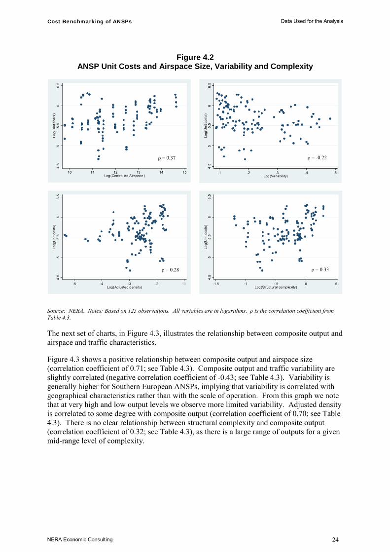
Figure 4.2 shows how ANSP unit costs are related to controlled airspace size, variability, density and complexity variables. These graphs allow us to investigate, descriptively, whether the heterogeneity of the operating environment across ANSPs plays a major role in determining the cost of providing a unit of output at a given scale of operations.
There is a weakly positive relationship between the size of controlled airspace and the unit costs (correlation coefficient of 0.37; see Table 4.3). The relationships between unit costs and either adjusted density or structural complexity are also weakly positive, while there is an even weaker (and negative) relationship between seasonal variability and unit costs (correlation coefficient of -0.22; see Table 4.3).
In all cases there are large differences in unit costs for given levels of each of the variables. This suggests that no single variable is able to explain a great proportion of the variance in unit costs across ANSPs. Therefore, either a combination of variables enters into the cost function in a potentially complex way, or there is a great deal of variation due to other factors (including inefficiency, but also variables that have not been identified but have an impact on unit costs).
ρ = 0.47 ρ = 0.98
Cost Benchmarking of ANSPs Data Used for the Analysis
NERA Economic Consulting 24
Figure 4.2 ANSP Unit Costs and Airspace Size, Variability and Complexity
4.5
55.
56
6.5
Log(
Uni
t cos
ts)
10 11 12 13 14 15Log(Controlled Airspace)
4.5
55.
56
6.5
Log(
Uni
t cos
ts)
.1 .2 .3 .4 .5Log(Variability)
4.5
55.
56
6.5
Log(
Uni
t cos
ts)
-5 -4 -3 -2 -1Log(Adjusted density)
4.5
55.
56
6.5
Log(
Uni
t cos
ts)
-1.5 -1 -.5 0 .5Log(Structural complexity)
Source: NERA. Notes: Based on 125 observations. All variables are in logarithms. ρ is the correlation coefficient from Table 4.3.
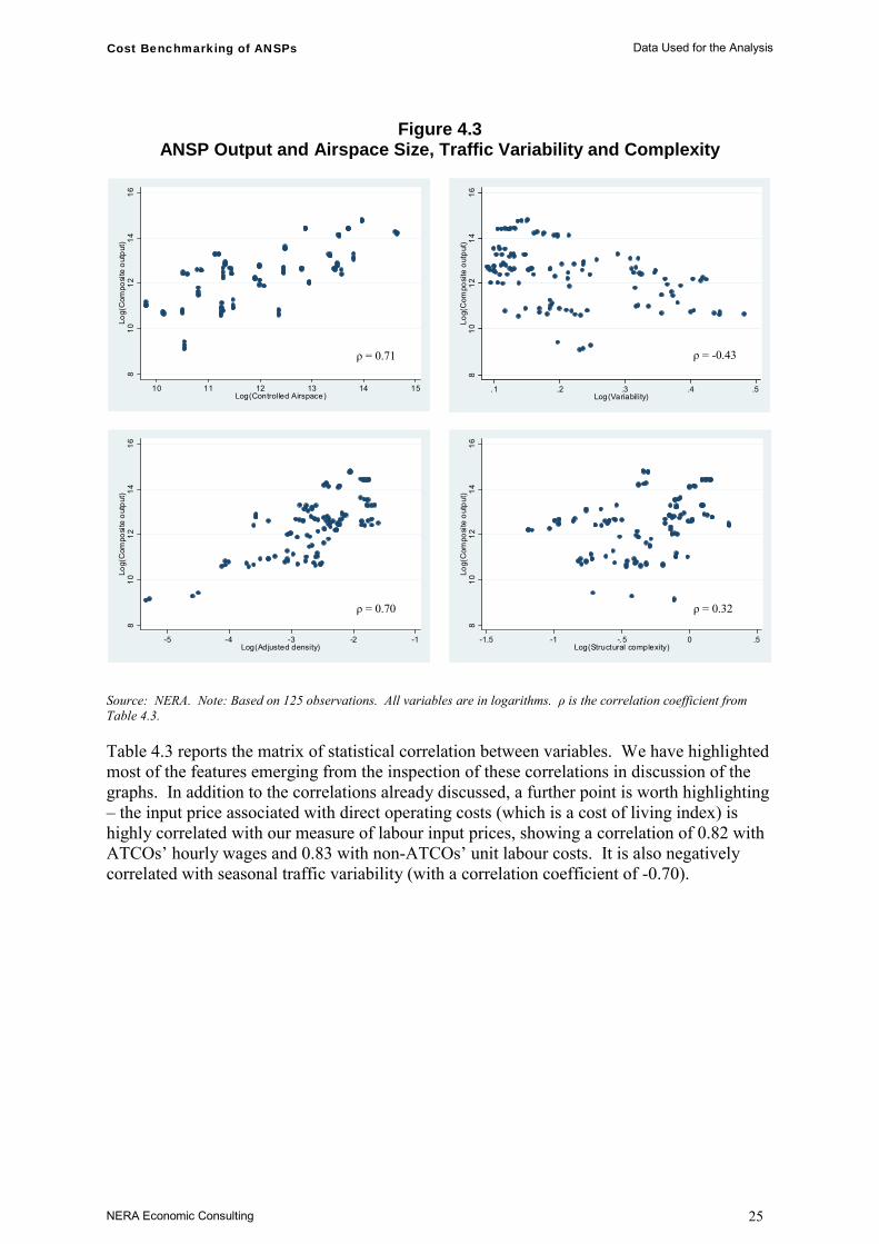
The next set of charts, in Figure 4.3, illustrates the relationship between composite output and airspace and traffic characteristics.
Figure 4.3 shows a positive relationship between composite output and airspace size (correlation coefficient of 0.71; see Table 4.3). Composite output and traffic variability are slightly correlated (negative correlation coefficient of -0.43; see Table 4.3). Variability is generally higher for Southern European ANSPs, implying that variability is correlated with geographical characteristics rather than with the scale of operation. From this graph we note that at very high and low output levels we observe more limited variability. Adjusted density is correlated to some degree with composite output (correlation coefficient of 0.70; see Table 4.3). There is no clear relationship between structural complexity and composite output (correlation coefficient of 0.32; see Table 4.3), as there is a large range of outputs for a given mid-range level of complexity.
ρ = -0.22 ρ = 0.37
ρ = 0.28 ρ = 0.33
Cost Benchmarking of ANSPs Data Used for the Analysis
NERA Economic Consulting 25
Figure 4.3 ANSP Output and Airspace Size, Traffic Variability and Complexity
810
1214
16Lo
g(C
ompo
site
out
put)
10 11 12 13 14 15Log(Controlled Airspace)
810
1214
16Lo
g(C
ompo
site
out
put)
.1 .2 .3 .4 .5Log(Variability)
810
1214
16Lo
g(C
ompo
site
out
put)
-5 -4 -3 -2 -1Log(Adjusted density)
810
1214
16Lo
g(C
ompo
site
out
put)
-1.5 -1 -.5 0 .5Log(Structural complexity)
Source: NERA. Note: Based on 125 observations. All variables are in logarithms. ρ is the correlation coefficient from Table 4.3.
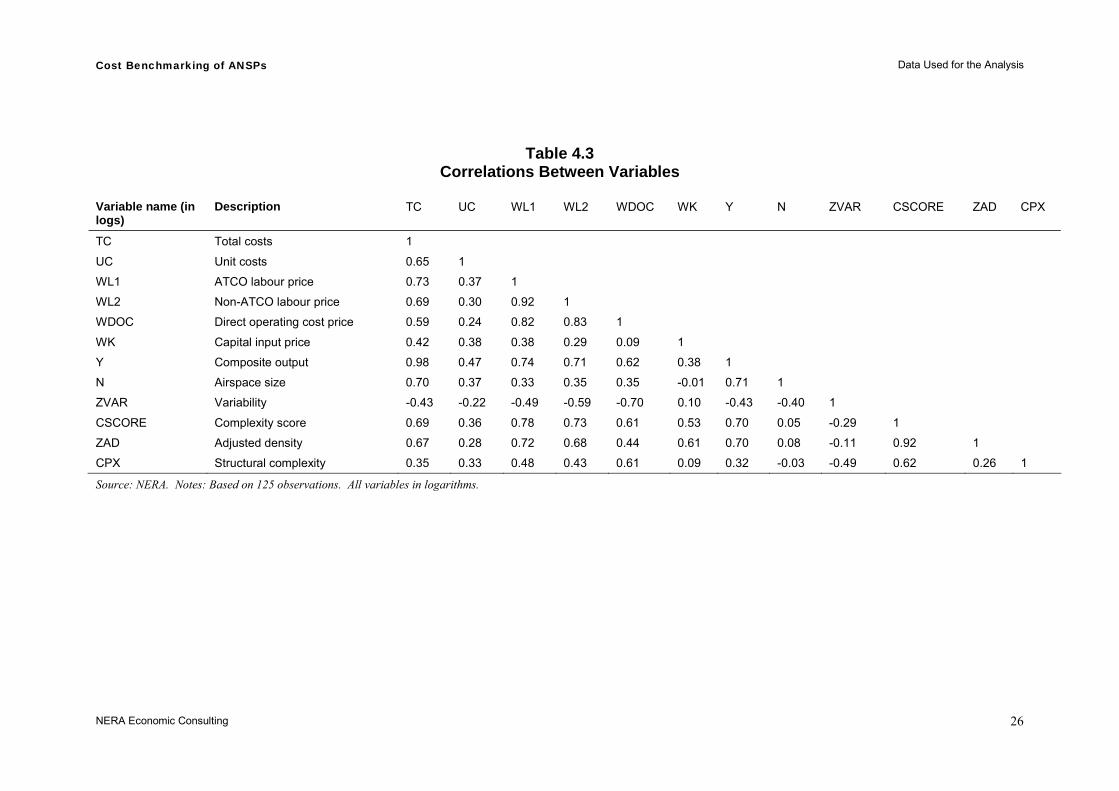
Table 4.3 reports the matrix of statistical correlation between variables. We have highlighted most of the features emerging from the inspection of these correlations in discussion of the graphs. In addition to the correlations already discussed, a further point is worth highlighting – the input price associated with direct operating costs (which is a cost of living index) is highly correlated with our measure of labour input prices, showing a correlation of 0.82 with ATCOs’ hourly wages and 0.83 with non-ATCOs’ unit labour costs. It is also negatively correlated with seasonal traffic variability (with a correlation coefficient of -0.70).
ρ = -0.43 ρ = 0.71
ρ = 0.70 ρ = 0.32
Cost Benchmarking of ANSPs Data Used for the Analysis
NERA Economic Consulting 26
Table 4.3 Correlations Between Variables
Variable name (in logs)
Description TC UC WL1 WL2 WDOC WK Y N ZVAR CSCORE ZAD CPX
TC Total costs 1
UC Unit costs 0.65 1
WL1 ATCO labour price 0.73 0.37 1
WL2 Non-ATCO labour price 0.69 0.30 0.92 1
WDOC Direct operating cost price 0.59 0.24 0.82 0.83 1
WK Capital input price 0.42 0.38 0.38 0.29 0.09 1
Y Composite output 0.98 0.47 0.74 0.71 0.62 0.38 1
N Airspace size 0.70 0.37 0.33 0.35 0.35 -0.01 0.71 1
ZVAR Variability -0.43 -0.22 -0.49 -0.59 -0.70 0.10 -0.43 -0.40 1
CSCORE Complexity score 0.69 0.36 0.78 0.73 0.61 0.53 0.70 0.05 -0.29 1
ZAD Adjusted density 0.67 0.28 0.72 0.68 0.44 0.61 0.70 0.08 -0.11 0.92 1
CPX Structural complexity 0.35 0.33 0.48 0.43 0.61 0.09 0.32 -0.03 -0.49 0.62 0.26 1
Source: NERA. Notes: Based on 125 observations. All variables in logarithms.
Cost Benchmarking of ANSPs Data Used for the Analysis
NERA Economic Consulting 27
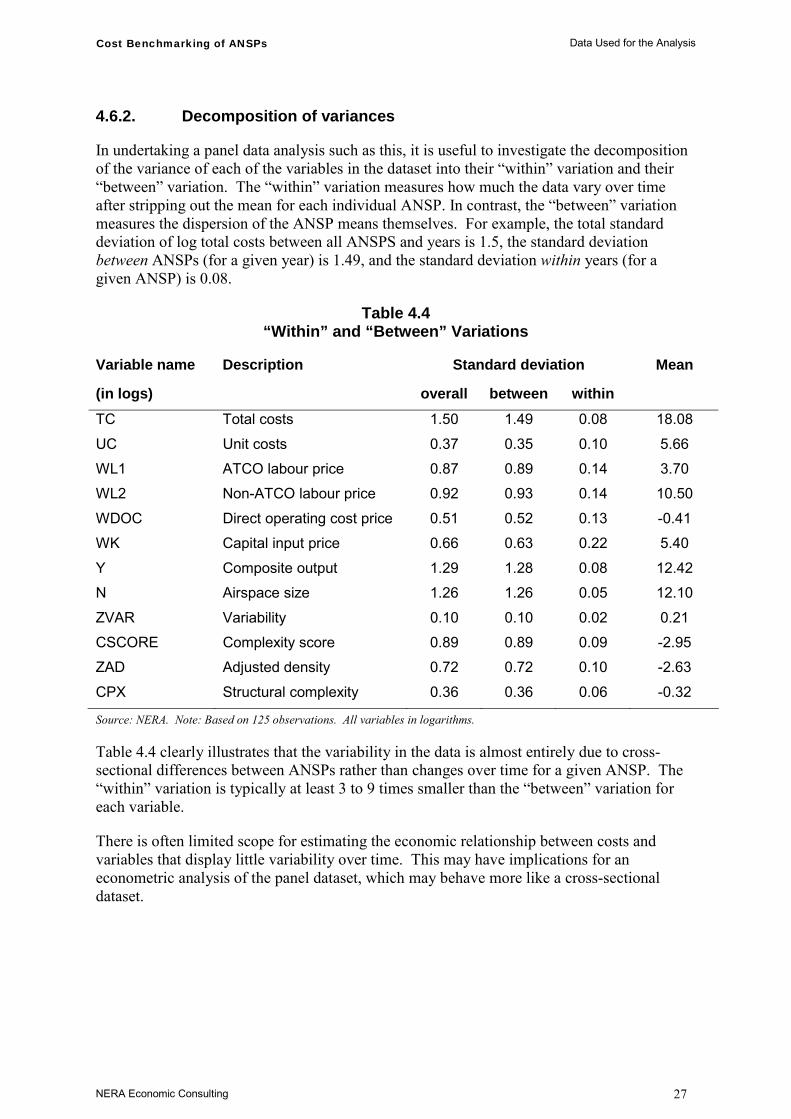
4.6.2. Decomposition of variances
In undertaking a panel data analysis such as this, it is useful to investigate the decomposition of the variance of each of the variables in the dataset into their “within” variation and their “between” variation. The “within” variation measures how much the data vary over time after stripping out the mean for each individual ANSP. In contrast, the “between” variation measures the dispersion of the ANSP means themselves. For example, the total standard deviation of log total costs between all ANSPS and years is 1.5, the standard deviation between ANSPs (for a given year) is 1.49, and the standard deviation within years (for a given ANSP) is 0.08.
Table 4.4 “Within” and “Between” Variations
Variable name Description Standard deviation Mean
(in logs) overall between within
TC Total costs 1.50 1.49 0.08 18.08
UC Unit costs 0.37 0.35 0.10 5.66
WL1 ATCO labour price 0.87 0.89 0.14 3.70
WL2 Non-ATCO labour price 0.92 0.93 0.14 10.50
WDOC Direct operating cost price 0.51 0.52 0.13 -0.41
WK Capital input price 0.66 0.63 0.22 5.40
Y Composite output 1.29 1.28 0.08 12.42
N Airspace size 1.26 1.26 0.05 12.10
ZVAR Variability 0.10 0.10 0.02 0.21
CSCORE Complexity score 0.89 0.89 0.09 -2.95
ZAD Adjusted density 0.72 0.72 0.10 -2.63
CPX Structural complexity 0.36 0.36 0.06 -0.32
Source: NERA. Note: Based on 125 observations. All variables in logarithms.
Table 4.4 clearly illustrates that the variability in the data is almost entirely due to cross-sectional differences between ANSPs rather than changes over time for a given ANSP. The “within” variation is typically at least 3 to 9 times smaller than the “between” variation for each variable.
There is often limited scope for estimating the economic relationship between costs and variables that display little variability over time. This may have implications for an econometric analysis of the panel dataset, which may behave more like a cross-sectional dataset.
Cost Benchmarking of ANSPs Econometric Model Specification
NERA Economic Consulting 28
5. Econometric Model Specification
In the present study, we adopt the parametric regression analysis approach to cost benchmarking. This approach requires assumptions regarding the shape of the cost frontier and the composition and distribution of the error term in order to differentiate between inefficiency and other factors. We begin this section by developing the econometric specification of an ANSP cost function. The remainder of the section then develops the specification further with respect to the decomposition of the error term into inefficiency and other components.
5.1. ANSP Cost Function
To estimate the cost functions in the present study, we adopt the Cobb-Douglas functional form (see Equations 5.1a and 5.1b below). This form has been widely used in empirical studies of cost functions and has the virtue of being simple to understand and analyse.
The Cobb-Douglas cost function is written as:
lnTC= α + β1lnWL1 + β2lnWL2 + β3lnWK + β4lnWDOC
+ φ lnY + δlnN + ω1lnZVAR + ω2lnCSCORE (5.1a)
where lnTC is the logarithm of total costs (see Table 4.2 for the definition of each variable). The parameters α, βj, φ, δ and ωk are to be estimated.
Alternatively, we have defined our model using a Cobb-Douglas cost function including the two disaggregated complexity metrics:
lnTC= α + β1lnWL1 + β2lnWL2 + β3lnWK + β4lnWDOC
+ φ lnY + δlnN + ω1lnZVAR + ω3lnZAD + ω4lnCPX (5.1b)
Since Equations 5.1a and 5.1b are log-linear, the parameters in the equation are all elasticities. Thus, for example, the βj parameters capture the percentage changes in total costs that would result from a change in each of the input prices.
In order to preserve linear homogeneity in input prices (ie if all input prices were to double then, all else equal, costs would also double), which is a theoretical requirement of cost functions, it is necessary to place a restriction on the equation. This restriction is that the sum of the βj parameters (ie the coefficients on input prices) must be equal to one.
The Cobb-Douglas functional form is simple and easy to interpret and it has relatively few parameters compared with other specifications – meaning the most important effects can be efficiently estimated. Its main disadvantage is that it is quite restrictive in terms of the shapes of cost function it allows the data to determine.
The most used flexible form of a cost function is the translog, introduced by Christensen, Jorgensen and Lau (1971). This functional form allows the data to drive the shape of the cost function with few restrictions and it allows multiple outputs to be included. Translog models, however, typically require a large number of observations to derive statistically significant estimates, due to the estimation of many more parameters (ie those relating to the squared and
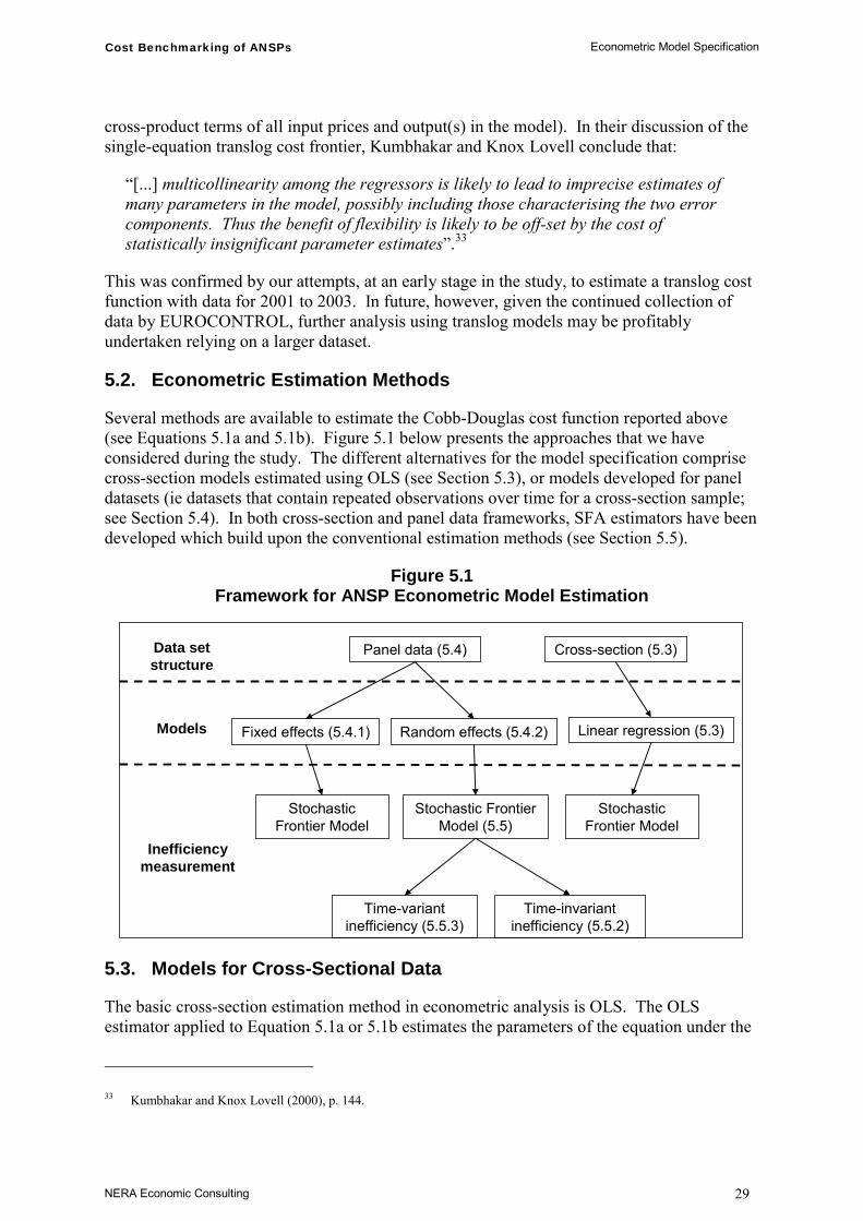
Cost Benchmarking of ANSPs Econometric Model Specification
NERA Economic Consulting 29
cross-product terms of all input prices and output(s) in the model). In their discussion of the single-equation translog cost frontier, Kumbhakar and Knox Lovell conclude that:
“[...] multicollinearity among the regressors is likely to lead to imprecise estimates of many parameters in the model, possibly including those characterising the two error components. Thus the benefit of flexibility is likely to be off-set by the cost of statistically insignificant parameter estimates”.33
This was confirmed by our attempts, at an early stage in the study, to estimate a translog cost function with data for 2001 to 2003. In future, however, given the continued collection of data by EUROCONTROL, further analysis using translog models may be profitably undertaken relying on a larger dataset.
5.2. Econometric Estimation Methods
Several methods are available to estimate the Cobb-Douglas cost function reported above (see Equations 5.1a and 5.1b). Figure 5.1 below presents the approaches that we have considered during the study. The different alternatives for the model specification comprise cross-section models estimated using OLS (see Section 5.3), or models developed for panel datasets (ie datasets that contain repeated observations over time for a cross-section sample; see Section 5.4). In both cross-section and panel data frameworks, SFA estimators have been developed which build upon the conventional estimation methods (see Section 5.5).
Figure 5.1 Framework for ANSP Econometric Model Estimation
Inefficiency measurement
Panel data (5.4) Cross-section (5.3)
Fixed effects (5.4.1) Random effects (5.4.2)
Stochastic Frontier Model
Stochastic Frontier Model (5.5)
Time-variant inefficiency (5.5.3)
Time-invariant inefficiency (5.5.2)
Stochastic Frontier Model
Models Linear regression (5.3)
Data set structure
5.3. Models for Cross-Sectional Data
The basic cross-section estimation method in econometric analysis is OLS. The OLS estimator applied to Equation 5.1a or 5.1b estimates the parameters of the equation under the
33 Kumbhakar and Knox Lovell (2000), p. 144.
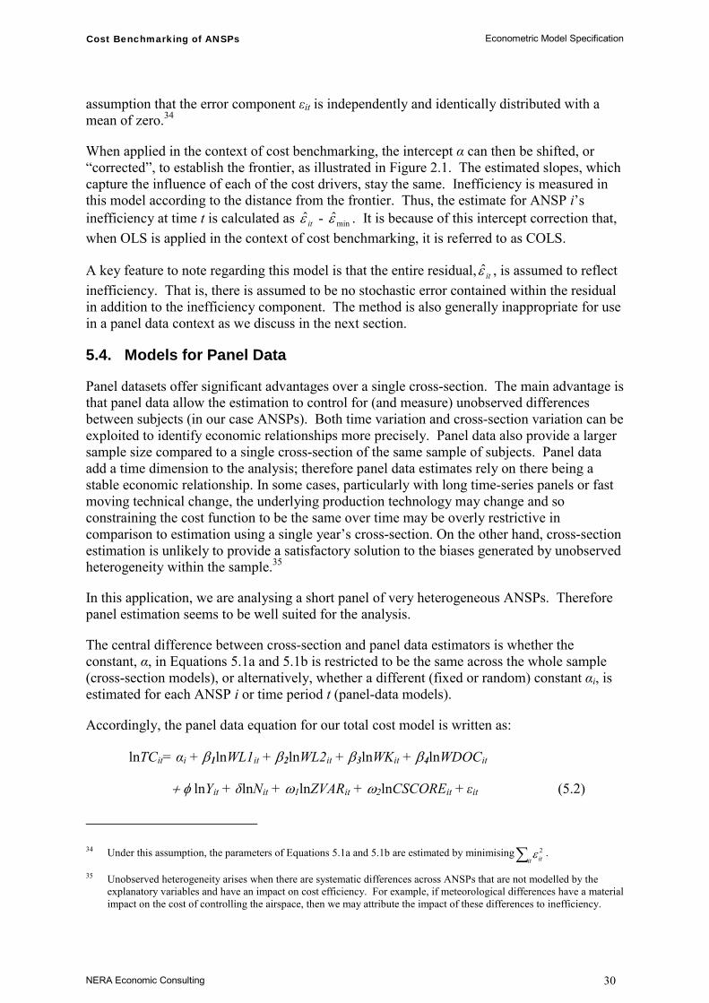
Cost Benchmarking of ANSPs Econometric Model Specification
NERA Economic Consulting 30
assumption that the error component εit is independently and identically distributed with a mean of zero.34
When applied in the context of cost benchmarking, the intercept α can then be shifted, or “corrected”, to establish the frontier, as illustrated in Figure 2.1. The estimated slopes, which capture the influence of each of the cost drivers, stay the same. Inefficiency is measured in this model according to the distance from the frontier. Thus, the estimate for ANSP i’s inefficiency at time t is calculated as itε̂ - minε̂ . It is because of this intercept correction that, when OLS is applied in the context of cost benchmarking, it is referred to as COLS.
A key feature to note regarding this model is that the entire residual, itε̂ , is assumed to reflect inefficiency. That is, there is assumed to be no stochastic error contained within the residual in addition to the inefficiency component. The method is also generally inappropriate for use in a panel data context as we discuss in the next section.
5.4. Models for Panel Data
Panel datasets offer significant advantages over a single cross-section. The main advantage is that panel data allow the estimation to control for (and measure) unobserved differences between subjects (in our case ANSPs). Both time variation and cross-section variation can be exploited to identify economic relationships more precisely. Panel data also provide a larger sample size compared to a single cross-section of the same sample of subjects. Panel data add a time dimension to the analysis; therefore panel data estimates rely on there being a stable economic relationship. In some cases, particularly with long time-series panels or fast moving technical change, the underlying production technology may change and so constraining the cost function to be the same over time may be overly restrictive in comparison to estimation using a single year’s cross-section. On the other hand, cross-section estimation is unlikely to provide a satisfactory solution to the biases generated by unobserved heterogeneity within the sample.35
In this application, we are analysing a short panel of very heterogeneous ANSPs. Therefore panel estimation seems to be well suited for the analysis.
The central difference between cross-section and panel data estimators is whether the constant, α, in Equations 5.1a and 5.1b is restricted to be the same across the whole sample (cross-section models), or alternatively, whether a different (fixed or random) constant αi, is estimated for each ANSP i or time period t (panel-data models).
Accordingly, the panel data equation for our total cost model is written as:
lnTCit= αi + β1lnWL1it + β2lnWL2it + β3lnWKit + β4lnWDOCit
+ φ lnYit + δlnNit + ω1lnZVARit + ω2lnCSCOREit + εit (5.2)
34 Under this assumption, the parameters of Equations 5.1a and 5.1b are estimated by minimising∑it it2ε .
35 Unobserved heterogeneity arises when there are systematic differences across ANSPs that are not modelled by the explanatory variables and have an impact on cost efficiency. For example, if meteorological differences have a material impact on the cost of controlling the airspace, then we may attribute the impact of these differences to inefficiency.
Cost Benchmarking of ANSPs Econometric Model Specification
NERA Economic Consulting 31
where lnTCit is the logarithm of total costs for ANSP i at time t; and αi, βj, φ, δ and ωk are parameters to be estimated; and εit is an error term that contains inefficiency and other random factors that have an impact on costs.
If Equation 5.2 is the true model, then estimating it using the standard OLS method with a single constant α will lead to biased estimates of the parameters αi, βj, φ, δ and ωk, and inefficiencies. This is illustrated in Figure 5.2.
Figure 5.2 Cross-Section and Panel Data Estimators when there is
Unobserved Heterogeneity
Output
Cost (C)
Panel:
Cross-section:
X
X
X
Output
Cost (C)
C=αi+φYit
Cross-
X
C=α+φYit
XX X
X XX
X X
In Figure 5.2, the four parallel lines represent the cost function as fitted by the panel data estimator and the single line with a different slope represents the cross-section estimator with a single constant term. The circled clusters of Xs represent observations on each ANSP in different years. From the way the figure is drawn, it is clear that the relationship between output and cost (ie the slope φ) is the same for all ANSPs but that the constants (α) are different, reflecting persistent, unobserved differences across ANSPs. Thus, when the constant is constrained to be the same across ANSPs, the resulting cost function slope is biased.
Panel data techniques encompass a range of alternative estimators. The main ones are fixed effects (FE) and random effects (RE) estimators. The key difference between these two estimators relates to whether the inefficiency error term is assumed to be uncorrelated with the explanatory variables (RE) or whether correlation is allowed (FE). We describe these two methods below, including how inefficiencies are estimated in each. We also discuss the economic implications of the assumptions on the correlation between inefficiency terms and explanatory variables.
5.4.1. Fixed effects (FE) model
In the FE model, the ANSP-specific constants αi in Equation 5.2 are estimated (and do not change over time). The model is estimated by including dummy variables Di, equal to 1 for
Cost Benchmarking of ANSPs Econometric Model Specification
NERA Economic Consulting 32
ANSP i and equal to 0 otherwise, in a regression, which is then estimated by OLS. The FE model is also known as the Least Squares Dummy Variables model for this reason.
An estimate for a time-invariant inefficiency term is calculated for each ANSP as the difference between the ANSP’s fixed effect ( iα̂ ) and the minimum fixed effect of all ANSPs in the sample ( minα̂ ). In the FE model the error term in Equation 5.2, εit is considered to be a stochastic error; therefore it does not contain any inefficiency. The method for separating inefficiency from stochastic error in this model assumes that all permanent time-invariant differences between ANSPs costs, after controlling for observed cost drivers, are due to inefficiency; and all deviations around the individual ANSP mean from year to year are stochastic error.36
An advantage of the FE model is that it requires very few assumptions to obtain consistent estimates of firm-specific inefficiency levels and all other parameters βj, φ, δ and ωk. All that is required is that εit are independently and identically distributed. Of particular importance is the fact that in the FE model, correlation (if any) between firm specific inefficiency dummies αi and explanatory variables does not bias estimates obtained via standard OLS. For example, the fact that the complexity of the airspace controlled by an ANSP might be positively correlated with its inefficiency level does not affect the consistency of OLS estimates (whereas it would affect the consistency of RE model estimates; see Section 5.4.2).
The drawback associated with the FE model, is that no time-invariant regressors can be included as explanatory variables.37 Also, the FE are intended to capture differences across ANSPs in time-invariant cost efficiency, but in practice they capture all time-invariant effects that vary across producers. RE models, in contrast, do allow for the inclusion of time-invariant explanatory variables. However, any remaining time-invariant unobserved heterogeneity would still be included in the inefficiency term.38 Also, RE models require additional distributional assumptions compared to FE models (ie the time-invariant inefficiency component must be uncorrelated with the explanatory variables).
In comparison with the COLS model, a further advantage of the FE model is that it allows for stochastic error as well as individual-specific inefficiency. The fact that the inefficiency estimate is assumed to be time-invariant may be considered either an advantage or a disadvantage. As an example, if inefficiency is mainly driven by managerial practice within ANSPs and different managerial practices/processes exist and persist over time across ANSPs, then the FE would be capturing persistent differences in managerial skill across ANSPs. If instead inefficiency is more volatile (thus changing substantially even within our four-year framework), than the FE estimator would average the year-specific inefficiencies for the whole time period analysed.
The data used in this study show considerably more variation between ANSPs than within ANSPs over time (see Table 4.4). The FE approach does not make especially good use of the data to identify the model parameters for variables that are somewhat time-invariant for
36 This method of estimating inefficiency using the fixed effects model is due to Schmidt and Sickles (1984). 37 See also Kumbhakar and Knox Lovell (2000), p.100. 38 See Greene (2002).
Cost Benchmarking of ANSPs Econometric Model Specification
NERA Economic Consulting 33
ANSPs. On this point, the RE model scores much better than the FE model, provided that one is willing to make stronger assumptions on the model structure.
5.4.2. Random effects (RE) model
As discussed in the previous section, the key feature of the RE model, which distinguishes it from the FE model, is its assumption that the αi are uncorrelated with the explanatory variables in the cost function. If one is comfortable with this assumption then the precision of the estimates can often be greatly improved by using the RE approach. This applies especially if, as is the case in the ANSP dataset, the majority of the variation in the explanatory variables is over the cross-section (ie between ANSPs) rather than over time. Kumbhakar and Knox Lovell (2000, p. 106) note that, provided the independence assumptions are met, RE models perform better than other models when there is a large cross section and a small number of time periods. It should also be noted that a large cross section is required for the consistency of the estimation of the variance of the inefficiency terms.39
Compared to the FE model, the RE approach has another advantage. Efficiency is estimated in the FE model relative to the “best” firm in the sample, which is equivalent to assuming that at least one firm is 100 per cent efficient. In the RE approach, in contrast, the inefficiency terms are measured in “absolute terms” (there no longer needs to be a 100 per cent efficient firm in the sample). Inefficiency levels measured via the RE in one sample group can thus be compared with RE inefficiency levels in another sample.
The conventional method for estimating the RE model is to use a Generalised Least Squares (GLS) procedure. This method, as the name suggests, is a generalised extension of OLS.40 The RE method results in parameter estimates that efficiently use time series and cross-section variation under the assumption that the individual-specific effects are independent of the explanatory variables. The standard RE model described above is not normally estimated in the context of cost benchmarking. Instead, SFA variants of this model are typically estimated using Maximum Likelihood (ML) methods, rather than GLS. These methods are described in the next section.
5.5. Stochastic Frontier Analysis
The first SFA model was developed in the context of production frontiers by Aigner et al. (1977). Schmidt and Knox Lovell (1979, 1980) extended this model to cost frontiers, and SFA has since been used extensively to estimate many types of model.
SFA models have been developed for cross-section and panel data frameworks. In this section we describe the general features of SFA models, before moving on to discuss the models we have estimated in this study. Furthermore, we have conducted a series of tests (not shown in the report) and concluded that the SFA specification is rejected in models that do not take account explicitly of the panel structure of the data.
39 Kumbhakar and Knox Lovell (2000), p. 101. 40 Unlike OLS, it does not require the errors to be independently and identically distributed, each with mean zero. Instead,
it allows for any error covariance matrix, including the random effects case where the error is assumed to comprise two components: an individual effect and a stochastic component.
Cost Benchmarking of ANSPs Econometric Model Specification
NERA Economic Consulting 34
5.5.1. General features of SFA
The key departure point for SFA models in relation to OLS regression methods is the inclusion of an asymmetric error term.
The error (ε it = v it + u it) is assumed to comprise two elements:
uit, which has a strictly non-negative distribution and represents the cost inefficiency component; and
vit, which has a symmetric distribution and represents stochastic error.
SFA models are estimated using the ML method. This method requires an assumption to be made concerning the shape of each of the error component distributions, in order to specify the Likelihood Function for the data sample as a function of the parameters to be estimated. The stochastic error is usually assumed to follow a normal distribution. Several alternative assumptions can be made, however, concerning the distribution of the non-negative disturbance component (uit). Generally the most common assumption is that of a half-normal distribution. This is based on the conjecture that the modal value of inefficiency (ie the most frequent level of inefficiency in the sample) is zero, and higher levels of inefficiency are less likely. Alternatively, one can assume that the one-sided error component is distributed as a truncated normal. The assumption of a truncated normal model allows more flexibility in the choice of the modal value for inefficiency (since it is not constrained to zero). This extension of the model can be relevant where the levels of inefficiency are known to be generally higher than zero (ie in very inefficient industries/countries).41
An important assumption that is maintained in these models is that the stochastic and the inefficiency components are both distributed independently of each other and of the regressors. The assumption of independence between the regressors and the error component is the most problematic assumption, since there may be good reasons why it may not hold. For example, one might believe that there are economies of scale available, but that larger firms tend to be less efficient than smaller firms. If this is the case then the assumption of independence is violated. Separating out the effects of inefficiency from technological cost drivers, when they are correlated, is not straightforward and may not be possible without making further identifying assumptions.
Assumptions about the distribution of the error terms seem to matter to the estimated size of the inefficiencies in an industry. However, the ranking of firms appears to be more robust and less sensitive to distributional assumptions.42
5.5.2. Random effects models with time-invariant inefficiency
The original RE estimator for SFA models, proposed by Pitt and Lee (1981), estimates individual-specific effects αi under the assumption that they are uncorrelated with the explanatory variables (see Section 5.4.2). In the SFA RE model, the individual time-
41 A further option is the normal exponential model, which assumes that the inefficiency term follows an exponential
distribution. Point estimates under this assumption are unbiased, but not consistent. In this report we do not discuss any results based on the exponential distribution.
42 For a discussion see, for example, Kumbhakar and Knox Lovell (2000).

Cost Benchmarking of ANSPs Econometric Model Specification
NERA Economic Consulting 35
invariant component is assumed to represent the individual’s (fixed) inefficiency, and it is assumed to follow a truncated-normal distribution. This model is estimated by ML and the estimate for inefficiency is calculated as E{exp(uit | εit )}.
This model, to some extent, carries the flavour of panel FE analysis, by assuming that there is a random time-persistent inefficiency specific to each individual ANSP. In addition, the stochastic error component, which is unrelated to inefficiency, can vary over time. Longer time panels mean the average of the stochastic error approaches zero, and the inefficiency estimate becomes more accurate.
5.5.3. Random effects models with time-varying inefficiency
The second SFA RE model, developed by Battesee and Coelli (1992), has inefficiency parametrically decaying or increasing over time at a constant rate. The rate is captured by a parameter η, assumed to be common across all firms. The Battesee-Coelli methodology models the error terms by including the inefficiency term (from a truncated-normal random variable) multiplied by a function of time:
u it = exp[-η*(t-T)]* ui
for individual i in year t, and T equal to the last time period in each panel. For example, the inefficiency of firm X in the first of four time periods of a panel dataset is:
u X1 = exp[-η*-3]* uX
The parameter η is to be estimated, and the uit are assumed to have a half-normal distribution. When η is positive the degree of inefficiency is decreasing over time. The inefficiency in the last period (where t is equal to T) represents the base level inefficiency for the firm, ui.
Setting η equal to 0 is equivalent to estimating a time-invariant model.
This model is more flexible than the time-invariant RE models, since ANSP-specific inefficiency is not constrained to be constant over time. However, the time-varying decay model can only account for monotonic trends in efficiency. If, for example, between 2001 and 2004 inefficiency in the overall sample initially increased but decreased at the end of the period, the time-decaying model will not reflect accurately these fluctuations in inefficiency over time.
5.5.4. Recent modelling innovations
In the FE model, described in Section 5.4.1, and the two SFA RE models, described in Section 5.5.2 and Section 5.5.3, all persistent unobserved heterogeneity in costs is considered to be inefficiency. This assumption may be too strong for ANSPs, where some of the causes of cost variation that are outside the control of the ANSP may be unobserved and/or not measured (either quantitatively or qualitatively). Whilst factors such as traffic variability and complexity are included in the cost function to capture differences in ANSPs’ operating environments, there are also likely to be missing factors (possibly such as corporate structure or regulatory framework), some of which may not be possible to include in a cost function. These factors typically do not change over a short time period and so are represented by ANSP-specific constants.
Cost Benchmarking of ANSPs Econometric Model Specification
NERA Economic Consulting 36
A number of estimators have been proposed more recently, which aim to distinguish individual-specific effects from inefficiency. Greene (2002) proposes models where an individual random fixed effect αi is added to the classical SFA RE specification.43 This method has two main shortcomings. The inclusion of the ANSP-specific fixed effect generates persistent biases when the number of periods is small (four is small). However Greene (2003) argues that these biases can be small. In addition, a separate (from the error term vit + uit) fixed effect αi might completely absorb persistent inefficiency in the ANSP-specific constant term (which is also capturing any time-invariant ANSP level heterogeneity). On this subject Greene (2003) argues that there is no entirely satisfactory way to disentangle firm-specific heterogeneity and inefficiency contained in αi +vit + uit. Both firm-specific inefficiency and heterogeneity can be considered a bundle of time-invariant and time-varying elements that cannot be perfectly disentangled based on available data. A model of this type, however, will systematically underestimate inefficiency if inefficiency is persistent (which is likely to be the case for many ANSPs).
Other recently suggested methods allow for a generalisation of the SFA RE model (eg Greene, 2002b and Greene, 2003) and address the independence requirements of the SFA RE model (eg Greene, Farsi and Filippini, 2005).
43 See, for example, a discussion in Greene (2003).

Cost Benchmarking of ANSPs Estimation of the Cost Function for ANSPs
NERA Economic Consulting 37
6. Estimation of the Cost Function for ANSPs
6.1. Our Approach
The econometric models have the total ATM/CNS costs as the dependent variable. The explanatory variables include the prices of two labour inputs (ATCOs and non-ATCOs), a direct operating input and a capital input (see Section 4.3 for more details); as well as network size, seasonal variability and complexity variables.
Our a priori inclination was towards the SFA RE time-varying model (see Section 5.5.3). First, we considered the adoption of a panel estimation method necessary due to the heterogeneity between ANSPs. Moreover, we thought that the econometric analysis should embody a time-decaying inefficiency component, reflecting a positive trend in efficiency across ANSPs over time. This is because cost pressures, regulatory scrutiny and technological advances are key factors that could contribute to a process of general efficiency improvement in the industry over time.
We tested a range of different econometric models, including cross-section SFA models (models in which the ANSP-specific effect is assumed to be zero). The results obtained show that cross-section models are less suited to estimating ANSP-specific cost inefficiency (relative to panel data models).44 This is in line with a priori expectations, given the level of heterogeneity relating to the various European ANSPs.
We then tested the cost function using a SFA FE model, but this yielded coefficients that had the “wrong” sign (ie a negative output coefficient). When we estimated the data using time-varying SFA RE, the model could not achieve convergence in STATA and so could not estimate ANSP inefficiencies. The years from 2002 to 2003 especially may be atypical because of the unexpected fall in air traffic. As a result, we decided to focus on the time-invariant SFA RE model because, at present, it is the model that encounters the least estimation problems compared to other panel data models.
Section 6.2 presents our main results from the SFA RE time-invariant model (introduced above in Section 5.5.2). Additional results from the SFA FE models (see Section 5.4.1) and SFA RE time-varying models (see Section 5.5.3) are shown in Appendix C.
6.2. Estimation Results
The main results for the time-invariant panel SFA model are presented in Table 6.1. Insignificant coefficients – meaning that statistical tests cannot prove, with a reasonable degree of confidence, that the true coefficient is not zero – are in grey. These estimates are likely to be unreliable. Point estimates of the significant coefficients are presented with an indication of the level of significance.
44 Our cross-section analysis also showed that there is no empirical evidence to suggest that the mean of the distribution of
the inefficiency error component differs from zero. Somewhat more promising results emerged from conditional mean cross-section SFA models, where the parameters of the density of the inefficiency error component depend on a set of environmental variables (that are not directly included in the cost function).
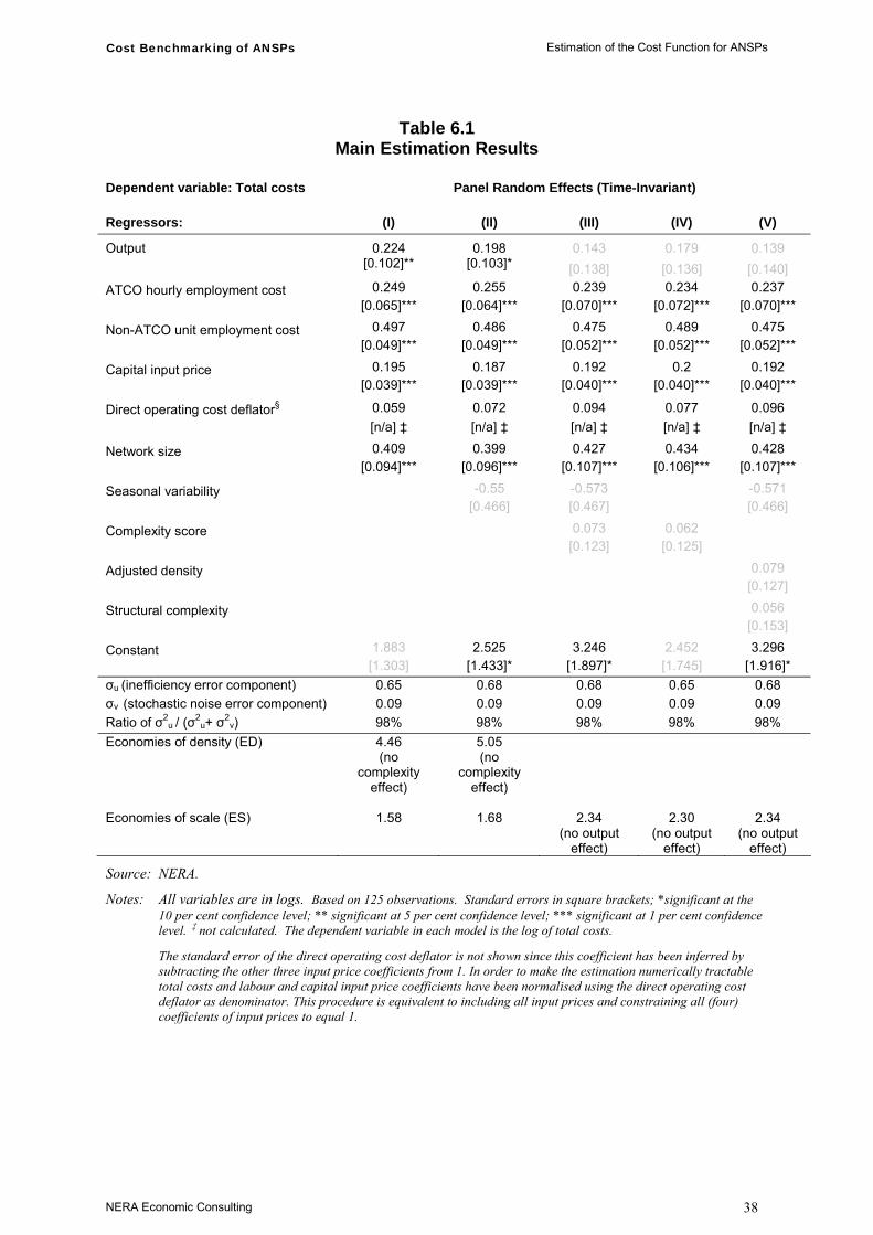
Cost Benchmarking of ANSPs Estimation of the Cost Function for ANSPs
NERA Economic Consulting 38
Table 6.1 Main Estimation Results
Dependent variable: Total costs Panel Random Effects (Time-Invariant)
Regressors: (I) (II) (III) (IV) (V)
Output 0.224 0.198 0.143 0.179 0.139 [0.102]** [0.103]* [0.138] [0.136] [0.140] ATCO hourly employment cost 0.249 0.255 0.239 0.234 0.237 [0.065]*** [0.064]*** [0.070]*** [0.072]*** [0.070]***
Non-ATCO unit employment cost 0.497 0.486 0.475 0.489 0.475 [0.049]*** [0.049]*** [0.052]*** [0.052]*** [0.052]***
Capital input price 0.195 0.187 0.192 0.2 0.192 [0.039]*** [0.039]*** [0.040]*** [0.040]*** [0.040]***
Direct operating cost deflator§ 0.059 0.072 0.094 0.077 0.096 [n/a] ‡ [n/a] ‡ [n/a] ‡ [n/a] ‡ [n/a] ‡
Network size 0.409 0.399 0.427 0.434 0.428 [0.094]*** [0.096]*** [0.107]*** [0.106]*** [0.107]***
Seasonal variability -0.55 -0.573 -0.571 [0.466] [0.467] [0.466]
Complexity score 0.073 0.062 [0.123] [0.125]
Adjusted density 0.079 [0.127]
Structural complexity 0.056 [0.153]
Constant 1.883 2.525 3.246 2.452 3.296 [1.303] [1.433]* [1.897]* [1.745] [1.916]* σu (inefficiency error component) 0.65 0.68 0.68 0.65 0.68 σv (stochastic noise error component) 0.09 0.09 0.09 0.09 0.09 Ratio of σ2
u / (σ2u+ σ2
v) 98% 98% 98% 98% 98% Economies of density (ED) 4.46
(no complexity
effect)
5.05 (no
complexity effect)
Economies of scale (ES) 1.58 1.68 2.34
(no output effect)
2.30 (no output
effect)
2.34 (no output
effect)
Source: NERA.
Notes: All variables are in logs. Based on 125 observations. Standard errors in square brackets; *significant at the 10 per cent confidence level; ** significant at 5 per cent confidence level; *** significant at 1 per cent confidence level. ‡ not calculated. The dependent variable in each model is the log of total costs.
The standard error of the direct operating cost deflator is not shown since this coefficient has been inferred by subtracting the other three input price coefficients from 1. In order to make the estimation numerically tractable total costs and labour and capital input price coefficients have been normalised using the direct operating cost deflator as denominator. This procedure is equivalent to including all input prices and constraining all (four) coefficients of input prices to equal 1.
Cost Benchmarking of ANSPs Estimation of the Cost Function for ANSPs
NERA Economic Consulting 39
Box 6.1 On the Interpretation of Significance Levels
The precision of the econometric estimation of a coefficient is summarised by the level of confidence at which the coefficient is significant. A standard threshold for the level of confidence is generally set at 5 per cent. The level of confidence is a measure of the probability that the true coefficient (which is not observable) is not within an interval of two standard errors on each side of the point estimation. This interval is called the confidence interval, ie a range of plausible values for the estimated coefficient. Therefore when a coefficient is estimated and found significant at the 1 per cent level of confidence, it means that the point estimation is very precise. On the other hand, a coefficient that is significant at the 10 per cent level of significance is less precisely estimated. Coefficients are considered insignificant when the 10 per cent level of significance has been exceeded (but many researchers adopt 5 per cent as a standard threshold). When coefficients are insignificant the standard error (relative to the coefficient size) is large; this means that the confidence interval for the estimated coefficient is wide, implying that there is a wider range of plausible estimates for a given coefficient compared to coefficients that are significant.
6.2.1. Interpretation of cost function coefficients
In Table 6.1, columns I to V show the results of five specifications of the SFA RE time-invariant model. Column I is an estimate of the basic model, while the next four include variables for seasonal variation, complexity score, adjusted density and structural complexity in various combinations.
As all variables are expressed in logarithms, the coefficients represent the elasticity of costs with respect to each independent variable. The output coefficient is statistically significant in columns I and II. Nonetheless, we consider the value of the coefficient to be too low. In particular, the coefficient estimates imply that there are huge economies of density in the provision of ANS provision (ie a 10 per cent increase in output, keeping the network size constant, results just in a 2 per cent increase in total costs). This low value could be due to multicollinearity, which can lead to inaccuracy in estimated coefficients, as output is relatively correlated with network size (correlation coefficient of 0.7; see Table 4.3).
In columns III to V, output is not statistically significant following the inclusion of different measures of traffic complexity. When the complexity score is included, the coefficient on output becomes smaller and the standard error wider; thus the point estimation of this coefficient is not significant. If taken at face value, this would lead to very large estimates of economies of density and scale. We believe that the smaller size of the coefficient is driven by the correlation between the output and the complexity score (correlation coefficient of 0.7; see Table 4.3) and the fact that output variations are mainly across ANSPs, rather than over time for a given ANSP. Also, we have included a time-invariant factor in the error. This is supported by the fact that, as shown in Appendix C, the FE model produces estimates of the output coefficient which are even less consistent with the theoretical expectations (being negative), and a more flexible time-varying inefficiency panel SFA model estimates output coefficients that are larger and more significant.
Cost Benchmarking of ANSPs Estimation of the Cost Function for ANSPs
NERA Economic Consulting 40
In all five specifications there is strong statistical evidence that the prices of ATCO and non-ATCO labour inputs, capital inputs and inputs associated with direct operating costs are significant drivers of total ANSP costs. The input price coefficients are relatively stable across the model specifications. The sum of the coefficients on labour input prices implies that the share of labour costs in total costs is about 72 per cent. This share is somewhat higher compared to the actual data (around 60 per cent; see Table 4.1).45
Our results suggest that a substantial share of unexplained variability is due to the ANSP-specific inefficiency error component. This is summarised by the ratio of the inefficiency-related residuals variance to the total residuals variance (σ2
u / (σ2u+ σ2
v)), which is shown at the bottom of Table 6.1. In columns I to V, 98 per cent of the unexplained variability is attributed to inefficiency. We infer from this that the ANSP inefficiencies are likely to be overestimated. We discuss the estimated inefficiency in Section 6.3.
6.2.2. Economies of scale and economies of density
Economies of scale:
In Table 6.1, an estimate of economies of scale, Es, is calculated using the sum of the cost elasticities with respect to output and with respect to network size, according to the formula: Es= [1/(φ + δ)], where φ is the coefficient on output and δ is the coefficient on network size. A value of Es greater than 1 implies economies of scale and a value less than 1 implies diseconomies of scale. The presence of economies of scale implies that, all else equal, total costs grow less than proportionally with increases in both output and network size.46
The economies of scale values are estimated to range between 1.58 and 2.34. The existence of economies of scale is determined by two factors:
the small increase in costs when output grows (the estimated coefficients on the output variable are 0.22 in column I and 0.20 in column II); and
the less than proportionate responsiveness of costs to changes in network size (the coefficient of network size is always positive and significant and ranges between 0.40 and 0.43).
However, we believe the output coefficient is too small and therefore the resulting estimates of economies of scale are unreliable.
Economies of density:
An estimate of economies of density, Ed, is calculated as [1/(φ +ω2 b1)] , where φ is the coefficient on output and ω2 is the coefficient on the overall complexity score. The parameter b1 measures the impact of output changes on complexity (while keeping network size fixed and all else equal) and has been estimated by the following auxiliary regression:47
45 Given the econometric specification of a Cobb-Douglas cost function, we would expect a priori that input price
coefficients would reflect actual cost shares. 46 See Appendix A for the derivation of the formula. 47 Network size is included in the auxiliary regression because both output and network size affect complexity. The
coefficient b1 therefore measures the change in complexity that arises from a change in output alone.

Cost Benchmarking of ANSPs Estimation of the Cost Function for ANSPs
NERA Economic Consulting 41
lnCSCOREit= a + b1 lnYit + b2 lnNit + eit
Therefore, Ed is composed of two elements. The first component, φ, captures the direct effect of output on total costs (when there is no change in network size). However, output has an additional indirect effect on costs through increased complexity. This is captured by the second component, ω2 b1, which is a compound of the effect of increased composite output on complexity (which we have estimated to correspond to an increase of 6.8 per cent when output rises by 10 per cent) and of the effect of the resulting increased complexity on costs. A value greater than 1 for Ed implies economies of density and a value lower than 1 implies diseconomies of density.48
In calculating Es and Ed we have interpreted any insignificant coefficients as zero.
Economies of density could only be calculated for models I and II since the estimated coefficients for output and complexity are both insignificant for the other models. In models I and II, the economies of density are a direct function of the estimated impact of output on costs. However, these measures of economies of density (4.46 and 5.05 for models I and II respectively) are overestimated because we are unable to calculate the indirect effect of an increase in output on complexity – since the coefficients are not statistically significant.
In all five model specifications in Table 6.1, the coefficients on the variability, density and complexity variables are not significant, even at the 10 per cent level. Moreover, inclusion of the density and complexity variables in the regression models results in output coefficients that are lower and less significant than those in models I and II. This may be due to multicollinearity, because of the relative correlation between the composite output and density and complexity measures (see Table 4.3).
6.3. Estimation of Cost Efficiency
In this section we present descriptive statistics and discuss the estimated cost efficiency scores for ANSPs. The efficiency score descriptive statistics in Table 6.2 are derived using model I from Table 6.1. This seemed to be the most appropriate specification for the full sample in terms of coefficient significance and magnitude.
48 See Appendix A for the derivation of the formula.
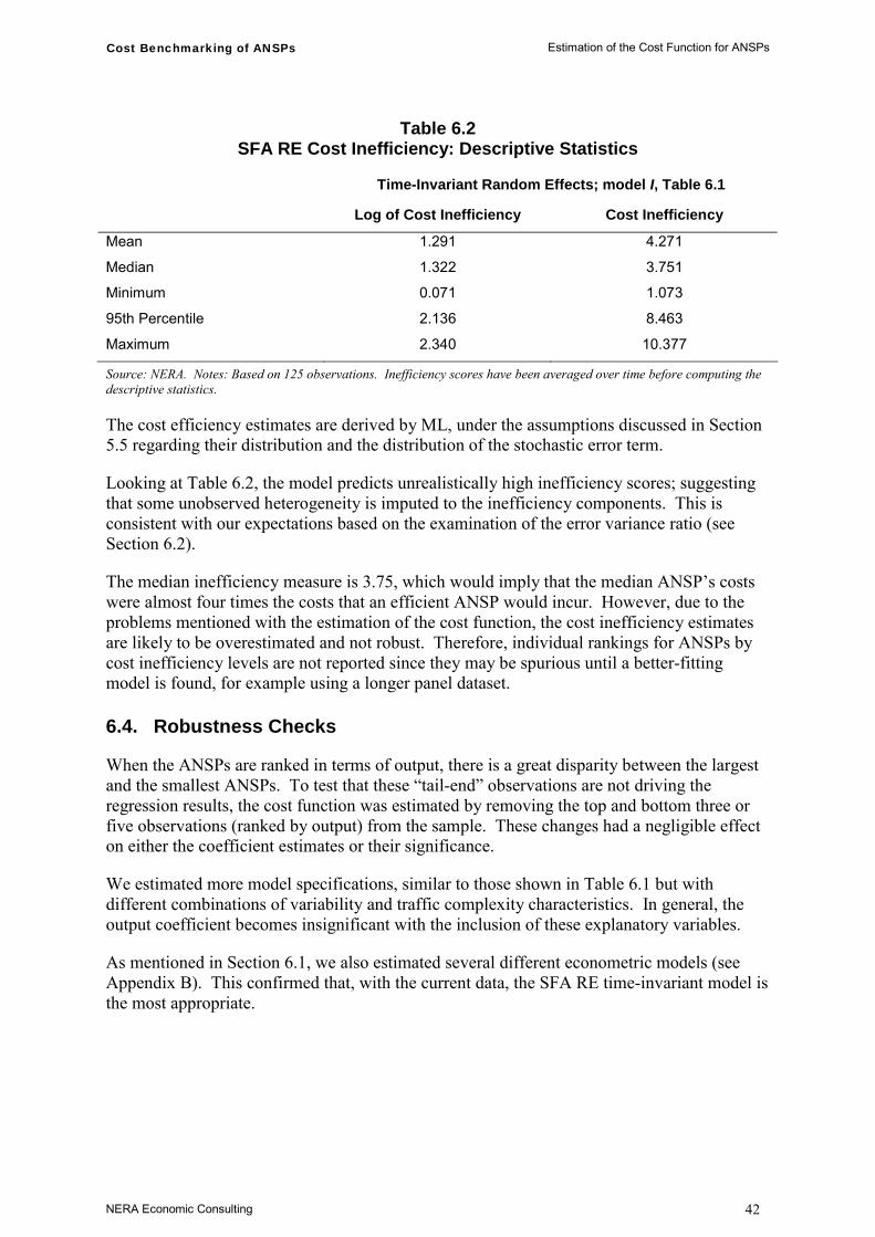
Cost Benchmarking of ANSPs Estimation of the Cost Function for ANSPs
NERA Economic Consulting 42
Table 6.2 SFA RE Cost Inefficiency: Descriptive Statistics
Time-Invariant Random Effects; model I, Table 6.1
Log of Cost Inefficiency Cost Inefficiency
Mean 1.291 4.271
Median 1.322 3.751
Minimum 0.071 1.073
95th Percentile 2.136 8.463
Maximum 2.340 10.377
Source: NERA. Notes: Based on 125 observations. Inefficiency scores have been averaged over time before computing the descriptive statistics.
The cost efficiency estimates are derived by ML, under the assumptions discussed in Section 5.5 regarding their distribution and the distribution of the stochastic error term.
Looking at Table 6.2, the model predicts unrealistically high inefficiency scores; suggesting that some unobserved heterogeneity is imputed to the inefficiency components. This is consistent with our expectations based on the examination of the error variance ratio (see Section 6.2).
The median inefficiency measure is 3.75, which would imply that the median ANSP’s costs were almost four times the costs that an efficient ANSP would incur. However, due to the problems mentioned with the estimation of the cost function, the cost inefficiency estimates are likely to be overestimated and not robust. Therefore, individual rankings for ANSPs by cost inefficiency levels are not reported since they may be spurious until a better-fitting model is found, for example using a longer panel dataset.
6.4. Robustness Checks
When the ANSPs are ranked in terms of output, there is a great disparity between the largest and the smallest ANSPs. To test that these “tail-end” observations are not driving the regression results, the cost function was estimated by removing the top and bottom three or five observations (ranked by output) from the sample. These changes had a negligible effect on either the coefficient estimates or their significance.
We estimated more model specifications, similar to those shown in Table 6.1 but with different combinations of variability and traffic complexity characteristics. In general, the output coefficient becomes insignificant with the inclusion of these explanatory variables.
As mentioned in Section 6.1, we also estimated several different econometric models (see Appendix B). This confirmed that, with the current data, the SFA RE time-invariant model is the most appropriate.

Cost Benchmarking of ANSPs Concluding Remarks
NERA Economic Consulting 43
7. Concluding Remarks
7.1. Lessons Learnt
On the basis of the evidence emerging from the econometric methodologies applied to the existing database, panel SFA analysis seems to be best suited to shed light on both ANSPs’ inefficiency and the relationship between output, input prices and costs. Panel techniques are very useful tools for the analysis of data from very heterogeneous ANSPs, since they exploit the variability over time to identify economic relationships over and above cross-section differences. They capture persistent individual ANSP features and estimate cost elasticities net of these ANSP-specific individual factors.
Among linear panel regression models, the FE model and the time-varying SFA RE model did not perform well, given the current dataset (see Appendix C). In the FE model, the output coefficient has the “wrong” sign and the network size coefficient is not statistically significant. Thus the model cannot be sensibly interpreted, and produces grossly overestimated economies of scale. The time-varying SFA RE model does not converge under any specification and thus the size and standard error of coefficient estimates may be biased, and it is not possible to compute cost inefficiencies. More years of data would be needed to produce a clearer monotonic trend (most likely of declining inefficiency).
Our favoured specification is the time-invariant SFA RE time-invariant model, which calculates an overall inefficiency for each ANSP given the four years of data. The seasonal variability, adjusted density and traffic complexity coefficients are not statistically significant. Moreover, their introduction in the model interacts with the estimation of the output coefficient, which becomes insignificant. However, a basic model of total costs regressed on output, input prices and network size produces coefficients that are significant, have the “right” sign and appear to be robust – though the output coefficient is lower than we might have expected (this could be due to multicollinearity, which can lead to inaccuracy in estimated coefficients, since the output and network size variables are relatively correlated). The cost inefficiencies seem to be overestimated; but this is expected given the empirical difficulties in distinguishing between ANSP heterogeneity and cost inefficiency under a short panel of data that varies little over time (and also perhaps because of unobserved heterogeneity). A longer panel of data would drive the stochastic error average towards zero, increasing the accuracy of the inefficiency estimate.
The fact that the variability, density and complexity variables were found to have no statistical power to explain cost differentials across ANSPs is a drawback of the time-invariant SFA RE model. This is almost certainly explained by the relatively small movement in these variables over the rather short (four years) sample time period.
7.2. Possible Directions for Future Research
7.2.1. A richer database
The analysis will benefit from a larger sample size and we understand that new data will be available each year. As additional years of data will be progressively added to the panel, it is possible that there will be sufficient variability in the regressors for a given ANSP to identify the effect of environmental characteristics over and above persistent individual differences, and to improve the performance of the three panel data models discussed in this paper. A

Cost Benchmarking of ANSPs Concluding Remarks
NERA Economic Consulting 44
larger dataset may also lead to improved results by allowing the application of more refined panel SFA techniques and more flexible cost function specifications, as discussed in the next two subsections.
7.2.2. New estimation methods
The obvious extension to the range of methodologies currently applied to this analysis is an SFA specification where three elements are included in the error term to provide a fuller characterization of inefficiency and heterogeneity – ie αi + uit + νit. 49 These elements are
ANSP specific FE, invariant over time (αi);
ANSP specific stochastic error terms (unrelated to inefficiency), varying over time (νit); and
ANSP specific asymmetric random inefficiency terms, allowed to vary over time (uit).
This is termed the “true” RE model (originally developed by Greene) and is used in empirical studies that include Greene (2003) and Farsi, Filipinni and Greene (2005). These studies examined panel data relating to health care and railways respectively. The main drawback is that persistent inefficiency may be absorbed by the fixed effect (ie persistent inefficiency is incorrectly assumed to be unobserved time-invariant heterogeneity between firms), and thus inefficiency is underestimated. This is likely to be a problem for estimating ANSPs’ cost inefficiencies since, a priori, we would expect much of the inefficiency to be persistent over time. However, application of the model in Farsi, Filipinni and Greene (2005) shows that there is some potential for improvements in the inefficiency estimation using the “true” RE model.
The results estimated with the “simple” FE model have highlighted the difficulties generated by a short panel with very heterogeneous ANSPs. A richer database can improve the results achieved with the methodologies explored so far, and could possibly provide sufficient variability in the data for simple FE and RE models and extensions to the RE model to perform well.
7.2.3. A more flexible functional form
A higher number of observations may also provide scope for achieving better results using a translog specification, even if the number of parameters that would be required (for example for a single output and four input prices model) will still be cumbersome for a sample twice as large as the current one. Our exploratory analysis using this functional form (not shown in this report) delivered very poor results. Particularly when there is a mix of significant and insignificant coefficients, the translog results may be difficult to interpret. However, a more flexible specification could offer improvements, for example if there were an underlying quadratic relationship between costs and output (which is one possible explanation why large ANSPs are currently ranked surprisingly low in our efficiency rakings). A translog cost function with just three input prices (using a single compounded input price for labour inputs and a similar index for capital inputs) might make the estimation more tractable.
49 One application of this model is discussed briefly in Section 5.5.4.
Cost Benchmarking of ANSPs Concluding Remarks
NERA Economic Consulting 45
7.2.4. New variables
7.2.4.1. Direct operating costs
Further work on the derivation of a more appropriate price index for direct operating costs, might help make the results of this cost efficiency exercise more dependable.
We have relied on a PPP-based cost-of-living index to approximate the input price associated with direct operating costs. However, this proxy for the prices of the services which make up direct operating costs might not capture real differences in relative prices across ANSPs/countries and it is clearly correlated with labour input prices. A possible direction of research (alternative to understanding the composition of these direct operating costs across ANSPs to identify the relevant inputs associated with these costs) is to identify a more specific industry price measure that may be less correlated with other input prices and the overall economic environment.
By using an industry specific price index we might:
rely on a better approximation of the cost of inputs associated with direct operating costs;50 and
rebalance the magnitude of the estimated input prices coefficients.
Further work might explore the potential to use sources such as Eurostat data (available online for most countries in our sample), which include various energy price indices and a communication index from 2001-2003.
Consideration of potential alternative price indices could also be informed by a more detailed understanding of the composition of direct operating costs across ANSPs. There may be a trade-off, for example, between the availability/reliability and relevance of particular indices. Information about the composition of these costs would also be useful in assessing the proportion that might be incurred at international (or regional) rather than domestic prices, and how this might be reflected in any revised index.
7.2.4.2. Capital costs and input prices
In order to calculate input prices for capital, we have used a weighted average of ACC sector-hours and ILS localisers as a proxy for physical capital inputs (these inputs have then been used to derive capital input prices from total capital costs). Future work could investigate possible improvements to both the measurement of total capital costs (which is subject to the difficulties discussed in Section 4.1) and also the derivation of an appropriate measure of input prices. As part of this, it could be useful to carry out further analysis of possible approaches to estimating the rental rate for capital inputs, rather than using physical measures as a proxy for the capital stock.
50 Thus, a priori, specific industry price indices seem to be more promising than the GDP deflator.

Cost Benchmarking of ANSPs Concluding Remarks
NERA Economic Consulting 46
7.2.4.3. A better understanding of unobserved heterogeneity
There are likely to be other characteristics of ANSPs and their operating environment that we have not captured, but which influence costs and are outside the control of managers and so should not be considered as inefficiency. If such factors are identified in future research, then they should be included in the analysis to provide a better characterisation of ANSPs’ performance.
Cost Benchmarking of ANSPs References
NERA Economic Consulting 47
8. References
EUROCONTROL Performance Review Unit
EUROCONTROL (2000) Progress Towards Cost-Benchmarking of the European ATM System
EUROCONTROL (2001) Progress Towards Cost-Benchmarking of the European ATM System: Update of the cost-benchmarking model for ANSPs/States in 1999
EUROCONTROL (2003a) A Comparison of Performance in Selected US and European En-Route Centres
EUROCONTROL (2003b) ATM Cost Effectiveness (ACE) 2001 Benchmarking Report
EUROCONTROL (2004) ATM Cost Effectiveness (ACE) 2002 Benchmarking Report
EUROCONTROL (2005a) ATM Cost Effectiveness (ACE) 2003 Benchmarking Report
EUROCONTROL (2005b) Total Factor Productivity of European Air Navigation Services Providers: Basic Concepts and Empirical Application, Draft Version 2.2, unpublished manuscript
EUROCONTROL (2005c) Complexity Metrics for ANSP Benchmarking Analysis
EUROCONTROL (2006) ATM Cost Effectiveness (ACE) 2004 Benchmarking Report
Academic
Aigner, D., C.A. Knox Lovell and P.Schmidt (1977), “Formulation and Estimation of Stochastic Frontier Production Function Models”, Journal of Econometrics 6:21-37
Bartels, R. and T. Islam (2002), “Supply Restricted Telecommunications Markets: The Effect of Technical Efficiency on Waiting Times,” Journal of Productivity Analysis 18:161-169
Battesee, G.E. and T.J. Coelli (1992) “Frontier Production Functions, Technical efficiency and Panel Data”, Journal of Productivity Analysis 3:153-169
Berger, A.N. and D.B. Humphrey (1997), “Efficiency of Financial Institutions: International Survey and Directions for Future Research”, European Journal of Operational Research 98:175-212
Burns, P. and T.G. Weyman-Jones (1996), “Cost Functions and Cost Efficiency in Electricity Distribution: A Stochastic Frontier Approach”, Bulletin of Economic Research 48(1):41-64
Chambers, R. (1988) Applied Production Analysis: A Dual Approach, Cambridge University Press
Christensen, Jorgensen and Lao (1971), “Conjugate Duality and the Transcendental Logarithmic Production Function”, Econometrica 39: 255-56

Cost Benchmarking of ANSPs References
NERA Economic Consulting 48
Coelli, T., S. Perelman, and E. Romano (1999), “Accounting for Environmental Influences in Stochastic Frontier Models: With Applications to International Airlines”, Journal of Productivity Analysis 11:251-274
Farsi, M., M. Filippini and M. Kuenzle (2005) “Unobserved Heterogeneity in Stochastic Cost Frontier Models: An Application to Swiss Nursing Homes”, Forthcoming in Applied Economics
Farsi, M., M. Filippini and W. Greene (2005) “Efficiency Measurement in Network Industries: Application to the Swiss Railway Companies”, Journal of Regulatory Economics 28(1):69-90
Farsi, M., M. Filippini and M. Kuenzle (2004) “Cost Efficiency of Regional Bus Companies: An Application of Alternative Stochastic Frontier Models”, forthcoming Journal of Transport Economics and Policy
Good, D. H., M.I. Nadiri, L.H. Röller and R. C. Sickles (1993), “Efficiency and productivity growth comparisons of European and U.S. air carriers: a first look at the data,” Journal of Productivity Analysis 4:115-125
Greene, W. (2002), “Alternative Panel Data Estimators for Stochastic Frontier Models”, mimeo
Greene, W. (2002b), “Fixed and Random Effects in Stochastic Frontier Models ”, mimeo
Greene, W. (2003), “Distinguishing Between Heterogeneity and Inefficiency: Stochastic Frontier Analysis of the World Health Organization’s Panel Data on National Health Care Systems,” Stern School of Business Working Paper, New York University
Greene, W. (2005), “Reconsidering Heterogeneity in Panel Data Estimators of the Stochastic Frontier Model”, Journal of Econometrics 126: 269-303
Kumbhakar, S.C. and C.A. Knox Lovell (2000), Stochastic Frontier Analysis. Cambridge University Press
Pitt, M. and L. Lee (1981) “The Measurement and Sources of Technical Inefficiency in Indonesian Weaving Industry”, Journal of Development Economics 9:43-64
Schmidt, P. and C.A. Knox Lovell (1979) “Estimating Technical and Allocative Inefficiency Relative to Stochastic Production and Cost Frontiers”, Journal of Econometrics 9:343-366
Schmidt, P. and C.A Knox Lovell (1980) “Estimating Stochastic Production and Cost Frontiers when Technical and Allocative Inefficiency are Correlated”, Journal of Econometrics 13(1): 83-100
Schmidt, P. and R. Sickles (1984) “Production Frontiers and Panel Data”, Journal of Business and Economic Statistics 2:367-374

Cost Benchmarking of ANSPs References
NERA Economic Consulting 49
Regulatory / Consulting / Air Traffic
Booz Allen Hamilton (2003) Study on Benchmarking for Best Practices in Air Traffic Management (European Community), Prepared for Directorate-General Energy and Transport
ICAO (2001) ICAO’s Policies on Charges for Airports and Air Navigation Services, Sixth Edition, Doc 9082/6
NERA (2001) Assessment of ATM Performance and Tariffs, A Report for ENAV
Solar Alliance and Steer Davies Gleeve (2005) Cost Benchmarking NATS Relative to Selected ANSPs: Final Report on Benchmarking with Existing Data, A Report for Civil Aviation Authority
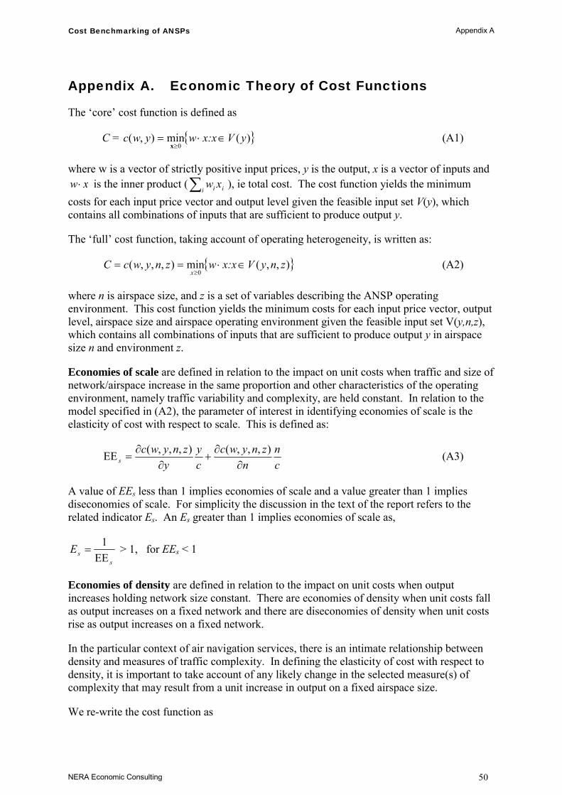
Cost Benchmarking of ANSPs Appendix A
NERA Economic Consulting 50
Appendix A. Economic Theory of Cost Functions
The ‘core’ cost function is defined as
C = { })(min),(0
yVx:xwywc ∈⋅=≥x
(A1)
where w is a vector of strictly positive input prices, y is the output, x is a vector of inputs and xw ⋅ is the inner product (∑i ii xw ), ie total cost. The cost function yields the minimum
costs for each input price vector and output level given the feasible input set V(y), which contains all combinations of inputs that are sufficient to produce output y.
The ‘full’ cost function, taking account of operating heterogeneity, is written as:
{ }),,(min),,,(0
znyVx:xwznywcCx
∈⋅==≥
(A2)
where n is airspace size, and z is a set of variables describing the ANSP operating environment. This cost function yields the minimum costs for each input price vector, output level, airspace size and airspace operating environment given the feasible input set V(y,n,z), which contains all combinations of inputs that are sufficient to produce output y in airspace size n and environment z.
Economies of scale are defined in relation to the impact on unit costs when traffic and size of network/airspace increase in the same proportion and other characteristics of the operating environment, namely traffic variability and complexity, are held constant. In relation to the model specified in (A2), the parameter of interest in identifying economies of scale is the elasticity of cost with respect to scale. This is defined as:
cn
nznywc
cy
yznywc
s ∂∂
+∂
∂=ΕΕ
),,,(),,,( (A3)
A value of ΕΕs less than 1 implies economies of scale and a value greater than 1 implies diseconomies of scale. For simplicity the discussion in the text of the report refers to the related indicator Es. An Es greater than 1 implies economies of scale as,
ssE
ΕΕ=
1 > 1, for ΕΕs < 1
Economies of density are defined in relation to the impact on unit costs when output increases holding network size constant. There are economies of density when unit costs fall as output increases on a fixed network and there are diseconomies of density when unit costs rise as output increases on a fixed network.
In the particular context of air navigation services, there is an intimate relationship between density and measures of traffic complexity. In defining the elasticity of cost with respect to density, it is important to take account of any likely change in the selected measure(s) of complexity that may result from a unit increase in output on a fixed airspace size.
We re-write the cost function as
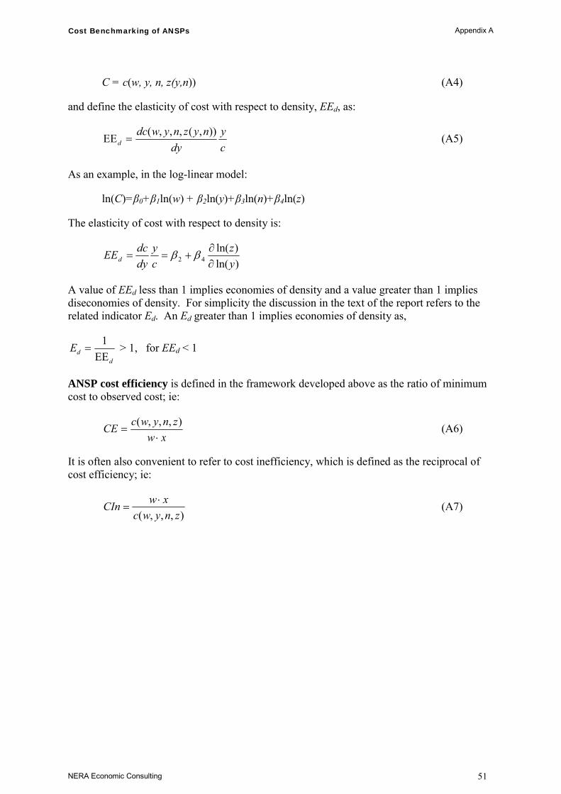
Cost Benchmarking of ANSPs Appendix A
NERA Economic Consulting 51
C = c(w, y, n, z(y,n)) (A4)
and define the elasticity of cost with respect to density, EEd, as:
cy
dynyznywdc
d)),(,,,(
=ΕΕ (A5)
As an example, in the log-linear model:
ln(C)=β0+β1ln(w) + β2ln(y)+β3ln(n)+β4ln(z)
The elasticity of cost with respect to density is:
)ln()ln(
42 yz
cy
dydcEEd ∂
∂+== ββ
A value of EEd less than 1 implies economies of density and a value greater than 1 implies diseconomies of density. For simplicity the discussion in the text of the report refers to the related indicator Ed. An Ed greater than 1 implies economies of density as,
ddE
ΕΕ=
1 > 1, for ΕΕd < 1
ANSP cost efficiency is defined in the framework developed above as the ratio of minimum cost to observed cost; ie:
xw
znywcCE⋅
=),,,( (A6)
It is often also convenient to refer to cost inefficiency, which is defined as the reciprocal of cost efficiency; ie:
),,,( znywc
xwCIn ⋅= (A7)

Cost Benchmarking of ANSPs Appendix B
NERA Economic Consulting 52
Appendix B. Stochastic Frontier Models
Our approach in the present study has been to estimate six main models, which differ in respect of the assumptions made concerning the firm-specific effect and/or the distribution of the components of the “composed error” εit. These models included three cross section specifications in addition to the three panel specifications for which results are reported in this paper. Table B.1 summarises the six main models estimated during the study.
Table B.1 Models used for SFA
Cross section data Panel data
Model A Half_norm
Model B Trunc_norm
Model C Trunc_cm
Model D FE
Model E RE
Model F RE_TD
Firm-specific component
none none none fixed (αi) uit=ui uit=exp{-η(t-Ti)ui}
Random error, εit εit = uit + vit uit ~ N+(0, σu
2) vit~ N(0, σv
2)
εit = uit + vit uit ~ N(μ, σu
2)vit~ N(0, σv
2)
εit = uit + vit uit~N+(μ(zit),σu
2)vit~ N(0, σv
2)
εit = vit vit~iidN(0, σv
2)
εit = ui + vit ui ~ N+( μ, σu
2) vit~ N(0, σv
2)
εit =exp{-η(t-Ti)ui}+vitui ~ N+(μ, σu
2) vit~ N(0, σv
2)
Inefficiency E[uit | uit+vit] E[uit | uit+vit]-μ
E[uit|uit+vit]- μ(zit)
}ˆmin{ˆ ii αα − E[ui|εi1, εi2,…] with εit = ui+vit
E(uit | uit + εit)
B.1. Cross Section Specifications
Models A and B are based on the assumptions of half-normal and truncated normal distributions of uit respectively. These models are estimated by maximum likelihood.51 The estimate for inefficiency is calculated as E(uit | εit) for Model A, while for Model B the truncated normal distribution, μ, is subtracted from E(uit | εit) to yield the estimate of inefficiency.
Model C removes the environmental variables from the cost function and instead uses them to condition the density of the inefficiency error component. This approach uses the information provided by the measures of traffic characteristics to explain the heterogeneity in the inefficiency term, rather than using the traffic characteristics directly in parameterising the cost frontier function. The mean of the inefficiency distribution, μ, is modelled as a linear combination of the set of covariates z. The model is estimated by maximising the same log-likelihood as in Model B, but in which ω'zit is substituted for μ. The log-likelihoods and estimators of inefficiency components for all models are contained in Section B.3.
In a study of international airlines’ efficiency, Coelli et al. (1999) find that these two models provide similar rankings52 but suggest differing degrees of technical inefficiency.
Our results for the cross section specifications found that the variance of the inefficiency component was negligible, ie all the variance in the error term was accounted for by the 51 The statistical package STATA was used to estimate all the models in this paper. 52 Generally they find that Asian/Oceanic airlines are more efficient than European and North American airlines but that
these differences are due to more favourable operating environments.
Cost Benchmarking of ANSPs Appendix B
NERA Economic Consulting 53
symmetric error component. This result was unsatisfactory. The results for the cross section specifications are not presented in this report.
B.2. Panel Specifications
Three panel specifications were estimated during the study. The first, Model D, is the FE model proposed by Schmidt and Sickles (1984). In this model, ANSP-specific constants are estimated and the disturbance term is assumed to be independently and identically distributed. The model coefficients are estimated using within-ANSP variation and cross-section variation. An estimate for a time-invariant inefficiency term is calculated for each ANSP in this model as the difference between the ANSP’s fixed effect and the minimum fixed effect of all ANSPs in the sample. Table B.2 shows the main advantages and disadvantages of the FE model.
Table B.2 Pros and Cons - FE Model
Inefficiency type Advantages Disadvantages
Time-invariant inefficiency
Unbiased inefficiency estimates can be calculated under few distributional assumptions
Unobserved environmental factors lead to overstated inefficiency
Firm-specific effects can be correlated with the explanatory variables
Inefficiency estimates are sensitive to outliers since no distributional assumptions, and one firm assumed to be “100 per cent efficient”
Inefficiency overstated since firm-specific effects absorb heterogeneous factors correlated with explanatory variables
Time-invariant explanatory variables cannot be included
Inefficiency assumed to be constant over time (although this can be an advantage)
The second panel specification, Model E, is the RE estimator proposed by Pitt and Lee (1981). This model estimates ANSP-specific effects αi under the assumption that they are uncorrelated with the explanatory variables. Model E is estimated by maximum likelihood. The estimate for inefficiency is calculated as E(uit | εit). Table B.3 shows the main advantages and disadvantages of the RE time-invariant model.
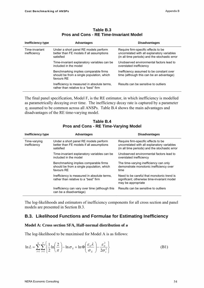
Cost Benchmarking of ANSPs Appendix B
NERA Economic Consulting 54
Table B.3 Pros and Cons - RE Time-Invariant Model
Inefficiency type Advantages Disadvantages
Time-invariant inefficiency
Under a short panel RE models perform better than FE models if all assumptions satisfied
Require firm-specific effects to be uncorrelated with all explanatory variables (in all time periods) and the stochastic error
Time-invariant explanatory variables can be included in the model
Unobserved environmental factors lead to overstated inefficiency
Benchmarking implies comparable firms should be from a single population, which favours RE
Inefficiency assumed to be constant over time (although this can be an advantage)
Inefficiency is measured in absolute terms, rather than relative to a “best” firm
Results can be sensitive to outliers
The final panel specification, Model F, is the RE estimator, in which inefficiency is modelled as parametrically decaying over time. The inefficiency decay rate is captured by a parameter η, assumed to be common across all ANSPs. Table B.4 shows the main advantages and disadvantages of the RE time-varying model.
Table B.4 Pros and Cons - RE Time-Varying Model
Inefficiency type Advantages Disadvantages
Time-varying inefficiency
Under a short panel RE models perform better than FE models if all assumptions satisfied
Require firm-specific effects to be uncorrelated with all explanatory variables (in all time periods) and the stochastic error
Time-invariant explanatory variables can be included in the model
Unobserved environmental factors lead to overstated inefficiency
Benchmarking implies comparable firms should be from a single population, which favours RE
The time-varying inefficiency can only demonstrate monotonic inefficiency over time
Inefficiency is measured in absolute terms, rather than relative to a “best” firm
Need to be careful that monotonic trend is significant; otherwise time-invariant model may be appropriate
Inefficiency can vary over time (although this can be a disadvantage)
Results can be sensitive to outliers
The log-likelihoods and estimators of inefficiency components for all cross section and panel models are presented in Section B.3.
B.3. Likelihood Functions and Formulae for Estimating Inefficiency
Model A: Cross section SFA, Half-normal distribution of u
The log-likelihood to be maximised for Model A is as follows:
∑∑= = ⎭
⎬⎫
⎩⎨⎧
−⎟⎟⎠
⎞⎜⎜⎝
⎛Φ+−⎟
⎠⎞
⎜⎝⎛=
N
i
T
t s
it
S
itSL
1 12
2
2lnln2ln
21ln
σε
σλε
σπ
(B1)

Cost Benchmarking of ANSPs Appendix B
NERA Economic Consulting 55
where ( ) 2122vuS σσσ += , vu σσλ = , and (.)Φ is the cumulative distribution function for the
standard normal distribution.
The estimate of inefficiency in this model is equal to:
( ) ( )( ) ⎭
⎬⎫
⎩⎨⎧
Φ−
+=**
****|
σμσμφ
σμεit
itititituE (B2)
where:
22* Suitit σσεμ = ; and,
Svu σσσσ =*
Model B: Cross Section SFA, Truncated-normal distribution of u
The log-likelihood to be maximised for Model B is:
( )( ){ }∑∑
= = ⎪⎭
⎪⎬⎫
⎪⎩
⎪⎨⎧
⎟⎟⎠
⎞⎜⎜⎝
⎛ −−
⎟⎟
⎠
⎞
⎜⎜
⎝
⎛
−
+−Φ+⎟
⎟⎠
⎞⎜⎜⎝
⎛Φ−−⎟
⎠⎞
⎜⎝⎛−=
N
i
T
t S
it
S
it
SSL
1 1
2
212 21
1
1lnlnln2ln
21ln
σμε
θθσ
θεμθθσ
μσπ
(B3)
Inefficiency is estimated in this model using (B3) above. However, in this case:
2
22
*S
vuitit σ
μσσεμ
+= ; and
Svu σσσσ =* .
Model C: Cross Section SFA, Truncated-normal distribution of u; with Conditioned Mean
In Model C, the mean parameter of the truncated normal distribution, μ, is modelled as a linear combination of the set of covariates z. The model is estimated by maximising the log-likelihood of equation (B3) above, wherein η'zit is substituted for μ.
Model E: Random Effects (Pitt and Lee, 1981)
The log-likelihood and inefficiency estimator for Model E are identical to those of Model F below, but wherein ρit = 1 and ρ = 0.
Model F: Random Effects, Time-Varying Inefficiency Model (Battese-Coelli, 1992)
The log-likelihood to be maximised for Model F is:
( ) ( ){ } ( ) ( )∑∑==
−−−+⎟⎠
⎞⎜⎝
⎛−=
N
iiS
N
ii TTL
1
2
1
1ln121ln2ln
21ln θσπ
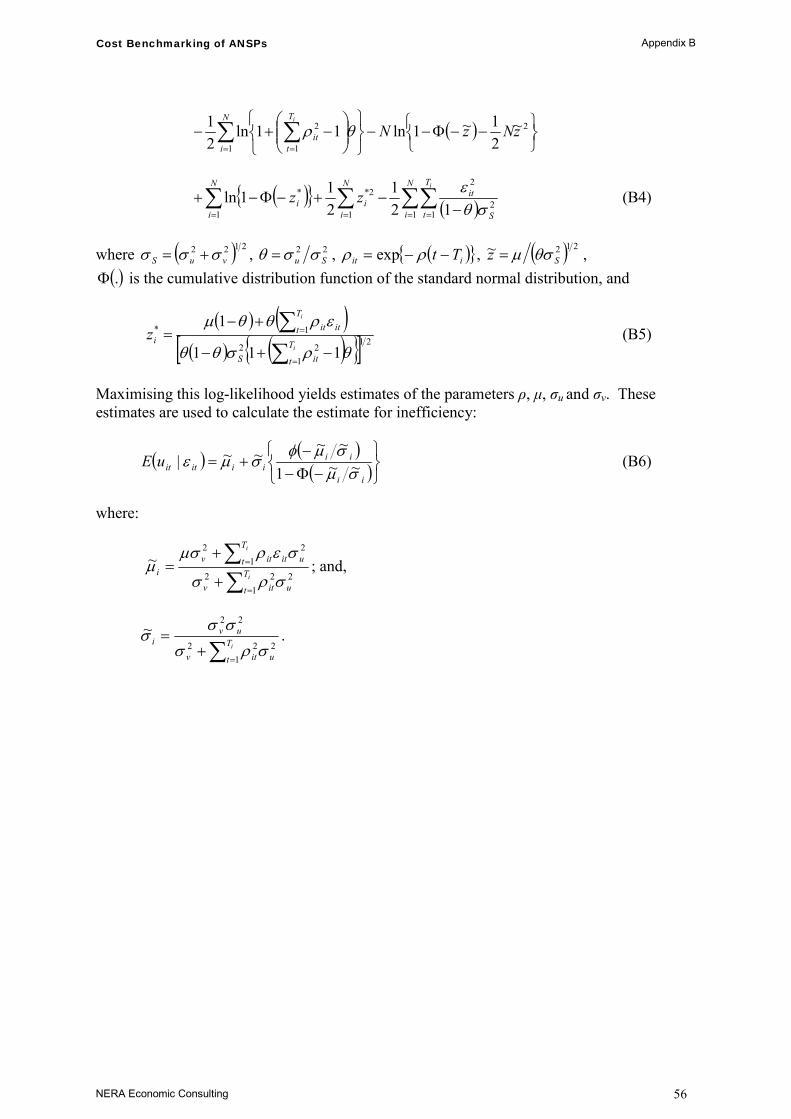
Cost Benchmarking of ANSPs Appendix B
NERA Economic Consulting 56
( )∑ ∑= = ⎭
⎬⎫
⎩⎨⎧ −−Φ−−
⎭⎬⎫
⎩⎨⎧
⎟⎟⎠
⎞⎜⎜⎝
⎛−+−
N
i
T
tit zNzN
i
1
2
1
2 ~21~1ln11ln
21 θρ
( ){ } ( )∑∑∑ ∑= == = −
−+−Φ−+N
i
T
t S
itN
i
N
iii
i
zz1 1
2
2
1 1
2**
121
211ln
σθε (B4)
where ( ) 2122vuS σσσ += , 22
Su σσθ = , ( ){ }iit Tt −−= ρρ exp , ( ) 212~Sz θσμ= ,
( ).Φ is the cumulative distribution function of the standard normal distribution, and
( ) ( )( ) ( ){ }[ ] 21
122
1*
111
1
θρσθθ
ερθθμ
−+−
+−=
∑∑
=
=
i
i
T
t itS
T
t ititiz (B5)
Maximising this log-likelihood yields estimates of the parameters ρ, μ, σu and σv. These estimates are used to calculate the estimate for inefficiency:
( ) ( )( )⎭
⎬⎫
⎩⎨⎧
−Φ−−
+=ii
iiiiitituE
σμσμφ
σμε ~~1
~~~~| (B6)
where:
∑∑
=
=
+
+=
i
i
T
t uitv
T
t uititvi
1222
122
~σρσ
σερμσμ ; and,
∑ =+
=iT
t uitv
uvi
1222
22~
σρσ
σσσ .
Cost Benchmarking of ANSPs Appendix C
NERA Economic Consulting 57
Appendix C. Econometric Estimates from the FE and the RE Time-Varying Models
This section presents the results from the regressions using the two alternative econometric models: the time-varying SFA RE model and the FE model. Section C.1 reports the coefficient estimates. The cost inefficiencies are not robust and have thus not been presented.
C.1. Main Econometric Estimates
Table C.1 reports the results of the SFA time-varying model regression set out in Section 5.5.3. Almost all of the specifications find input prices and output as significant drivers of costs. On the other hand, seasonality and complexity indicators (both aggregated as complexity score or disaggregated in its two components) fail to be estimated significantly. However, the estimation process in STATA failed to achieve convergence, meaning that the coefficients’ magnitude and standard errors may be biased. In addition to casting doubt on the reliability of the results shown in Table C.1, we could not calculate inefficiencies for this model.
These results would suggest that economies of scale are present as the joint impact of output and network size on costs is positive but less than proportional (as shown by the sum of the elasticities). Moreover, output drives the economies of density through its direct impact on costs, while the lack of significance of complexity implies that no indirect output effect affects the economies of density indicator.
Taking the estimates at face value, we notice that the output coefficient is higher than in the SFA RE time-invariant specification. Therefore, it provides a more acceptable estimate of economies of density. On the other hand, the ATCO labour costs coefficient and the sum of all labour cost coefficients are below what is expected given the analysis of actual cost shares in ANSPs. This results in a significantly higher estimate of the direct operating cost coefficient than in the SFA RE time-invariant model. Overall, given these problems and the fact that the model could not converge in STATA, the SFA RE time-varying model is not suitable given the small dataset.

Cost Benchmarking of ANSPs Appendix C
NERA Economic Consulting 58
Table C.1 Main Estimation Results: Random Effects Time-Varying Model
Dependent variable: Total Costs
Panel Random Effects (Time-Varying)
Regressors: (I) (II) (III) (IV) (V) Output 0.488 0.492 0.644 0.63 0.644 [0.089]*** [0.093]*** [0.132]*** [0.127]*** [0.134]*** ATCO hourly employment cost 0.098 0.097 0.125 0.128 0.125 [0.059]* [0.061] [0.063]** [0.062]** [0.063]** Non-ATCO unit employment cost 0.272 0.272 0.281 0.282 0.281 [0.053]*** [0.053]*** [0.053]*** [0.053]*** [0.053]*** Capital input price 0.179 0.179 0.166 0.164 0.166 [0.033]*** [0.033]*** [0.034]*** [0.033]*** [0.034]*** Direct operating cost deflator 0.451 0.452 0.428 0.426 0.428
[n/a] ‡ [n/a] ‡ [n/a] ‡ [n/a] ‡ [n/a] ‡ Network size 0.248 0.248 0.164 0.166 0.164 [0.079]*** [0.079]*** [0.094]* [0.094]* [0.094]* Seasonal variability 0.058 0.152 0.151 [0.414] [0.412] [0.412] Complexity score -0.177 -0.171 [0.110] [0.108] Adjusted density -0.176 [0.114] Structural complexity -0.179 [0.132] Constant -452.676 -413.835 -596.831 -550.706 -445.687 [1.108]*** [1.189]*** [1.492]*** [1.405]*** [1.509]*** σu (inefficiency error component) 0.51 0.51 0.5 0.51 0.5 σv (stochastic noise error component)
0.07 0.07 0.07 0.07 0.07
Ratio of σ2u / (σ2
u+ σ2v) 98% 98% 98% 98% 98%
Economies of density (ED) 2.05 (no
complexity effect)
2.03 (no
complexity effect)
1.55 (no
complexity effect)
1.59 (no
complexity effect)
1.55 (no
complexity effect)
Economies of scale (ES) 1.36 1.35 1.24 1.26 1.24
Source: NERA.
Notes: All variables are in logs. Based on 125 observations. Standard errors in square brackets; *significant at the 10 per cent confidence level; ** significant at 5 per cent confidence level; *** significant at 1 per cent confidence level. The dependent variable in each model is the log of total costs.
The formula used to calculate the estimated economies of scale, ES, is [1/(φ+δ)], where φ is the coefficient on output and δ is the coefficient on network size. ED are the estimated economies of density, equal to [1/(φ +0.68 ω2)], where ω2 is the coefficient on traffic complexity score and 0.68 is the estimated coefficient on output from an auxiliary regression of traffic complexity on output and network size. Insignificant coefficients have been treated as zero. ‡ The standard error of the direct operating cost deflator is not shown since this coefficient has been inferred by subtracting the other four input price coefficients from 1. In order to make the estimation numerically tractable total costs and labour and capital input price coefficients have been normalised using the direct operating cost deflator as denominator. This procedure is equivalent to including all input prices and constraining all (four) coefficients of input prices to equal 1.
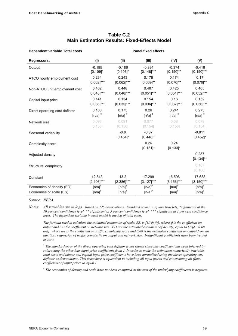
Cost Benchmarking of ANSPs Appendix C
NERA Economic Consulting 59
Table C.2 Main Estimation Results: Fixed-Effects Model
Dependent variable Total costs Panel fixed effects
Regressors: (I) (II) (III) (IV) (V)
Output -0.185 -0.186 -0.391 -0.374 -0.416 [0.109]* [0.108]* [0.148]*** [0.150]** [0.150]***
ATCO hourly employment cost 0.234 0.243 0.179 0.174 0.17 [0.062]*** [0.062]*** [0.069]** [0.070]** [0.070]**
Non-ATCO unit employment cost 0.462 0.448 0.407 0.425 0.405 [0.048]*** [0.048]*** [0.051]*** [0.051]*** [0.052]***
Capital input price 0.141 0.134 0.154 0.16 0.152 [0.036]*** [0.035]*** [0.036]*** [0.037]*** [0.036]***
Direct operating cost deflator 0.163 0.175 0.26 0.241 0.273 [n/a] ‡ [n/a] ‡ [n/a] ‡ [n/a] ‡ [n/a] ‡
Network size 0.093 0.091 0.077 0.08 0.079 [0.158] [0.156] [0.154] [0.156] [0.154]
Seasonal variability -0.8 -0.87 -0.811 [0.454]* [0.448]* [0.452]*
Complexity score 0.26 0.24 [0.131]* [0.133]*
Adjusted density 0.287
[0.134]**
Structural complexity 0.167
[0.160]
Constant 12.843 13.2 17.299 16.598 17.688 [2.406]*** [2.386]*** [3.127]*** [3.156]*** [3.150]*** Economies of density (ED) [n/a]# [n/a]# [n/a]# [n/a]# [n/a]# Economies of scale (ES) [n/a]# [n/a]# [n/a]# [n/a]# [n/a]#
Source: NERA.
Notes: All variables are in logs. Based on 125 observations. Standard errors in square brackets; *significant at the 10 per cent confidence level; ** significant at 5 per cent confidence level; *** significant at 1 per cent confidence level. The dependent variable in each model is the log of total costs.
The formula used to calculate the estimated economies of scale, ES, is [1/(φ+δ)], where φ is the coefficient on output and δ is the coefficient on network size. ED are the estimated economies of density, equal to [1/(φ +0.68 ω2)], where ω2 is the coefficient on traffic complexity score and 0.68 is the estimated coefficient on output from an auxiliary regression of traffic complexity on output and network size. Insignificant coefficients have been treated as zero. ‡ The standard error of the direct operating cost deflator is not shown since this coefficient has been inferred by subtracting the other four input price coefficients from 1. In order to make the estimation numerically tractable total costs and labour and capital input price coefficients have been normalized using the direct operating cost deflator as denominator. This procedure is equivalent to including all input prices and constraining all (four) coefficients of input prices to equal 1. # The economies of density and scale have not been computed as the sum of the underlying coefficients is negative.

Cost Benchmarking of ANSPs Appendix C
NERA Economic Consulting 60
Table C.2 reports the results of the regression of the FE model set out in Section 5.4.1. The coefficient estimates raise concerns. Our findings show that, using this methodology, all input prices are identified as significant drivers of costs, together with output. But most noticeably, the estimates present us with a negative coefficient for output. This is equivalent to stating that overall costs would actually decrease when output increases, which is obviously spurious.
Moreover, the coefficient on seasonal variability is negative. This runs counter to our intuition that a more seasonal pattern of traffic leads to higher costs, as a relatively large labour force (and capital stock) needs to be maintained throughout the year in order to ensure that sufficient capacity is available in the peak.
Finally, some complexity indicators are significant when introduced. In particular this refers to the complexity score and to its adjusted density component. Hence, while these econometric estimates do not confirm the structural complexity dimension as a cost driver, they do instead highlight adjusted density as a factor affecting total costs. Any estimates of economies of scale and density would be misleading because of the negative output coefficients, so they are not calculated.
We conclude that the inclusion of ANSP-specific fixed effect dummies has captured most of the heterogeneity across ANSPs, “absorbing” the FE important cost drivers such as network size and traffic complexity (due to the fact that these variables have changed only slightly during our four year sample period).

NERA Economic Consulting 61
NERA Economic Consulting 15 Stratford Place London W1C 1BE United Kingdom Tel: +44 20 7659 8500 Fax: +44 20 7659 8501 www.nera.com
NERA UK Limited, registered in England and Wales, No 3974527 Registered Office: 15 Stratford Place, London W1C 1BE