METHODOLOGY AND APPLICATIONS OF STOCHASTIC FRONTIER ANALYSISSTOCHASTIC FRONTIER ANALYSIS

Andrea Furková

STRUCTURE OF THE PRESENTATIONPart 1Theory: Illustration the basics of Stochastic

Frontier Analysis (SFA)– Concept of efficiency

– Estimation– Estimation

– Identification of sources of inefficiency

Part 2An applications of SFA

• Theory usually presents the producers as successfuloptimizers. They maximize production, minimizecost, and maximize profits.

• Conventionaleconometrictechniquesbuild on this• Conventionaleconometrictechniquesbuild on thisbase to estimate production/cost/profit functionparameters using regression techniques wheredeviations of observed choices fromoptimal ones aremodeled as statistical noise.

Econometric estimation techniques should allowforthe fact that deviations of observed choices fromoptimal ones are due to two factors:

• failure to optimize i.e., inefficiency• due to randomshocks.

Stochastic Frontier Analysis is one such techniqueto model producer behavior.

Methods based on efficient frontier

• Based on benchmarking, that is, a unit’sperformance is compared with a referenceperformance (so-called efficient frontier).

• Unit’s inefficiency canresultsfrom technological• Unit’s inefficiency canresultsfrom technologicaldeficiencies (technical inefficiency) or non-optimal allocation of resources into production(allocative inefficiency). Both technical andallocative inefficiencies are included in cost(economic) inefficiency.

Generally, there are two families of methods based on efficient frontier:

• Non-parametric methods, like Data EnvelopmentAnalysis (DEA) or Free Disposal Hull (FDH). Thesemethodsoriginatefrom operationsresearchanduselinearprogrammingto calculateanefficient deterministicfrontiermethodsoriginatefrom operationsresearchanduselinearprogrammingto calculateanefficient deterministicfrontieragainst which units are compared.

• Parametric methods, like Stochastic Frontier Analysis(SFA), Thick Frontier Approach (TFA) and DistributionFree Approach (DFA). Econometric theory is used toestimate pre-specified functional formand inefficiency ismodeled as an additional stochastic term.

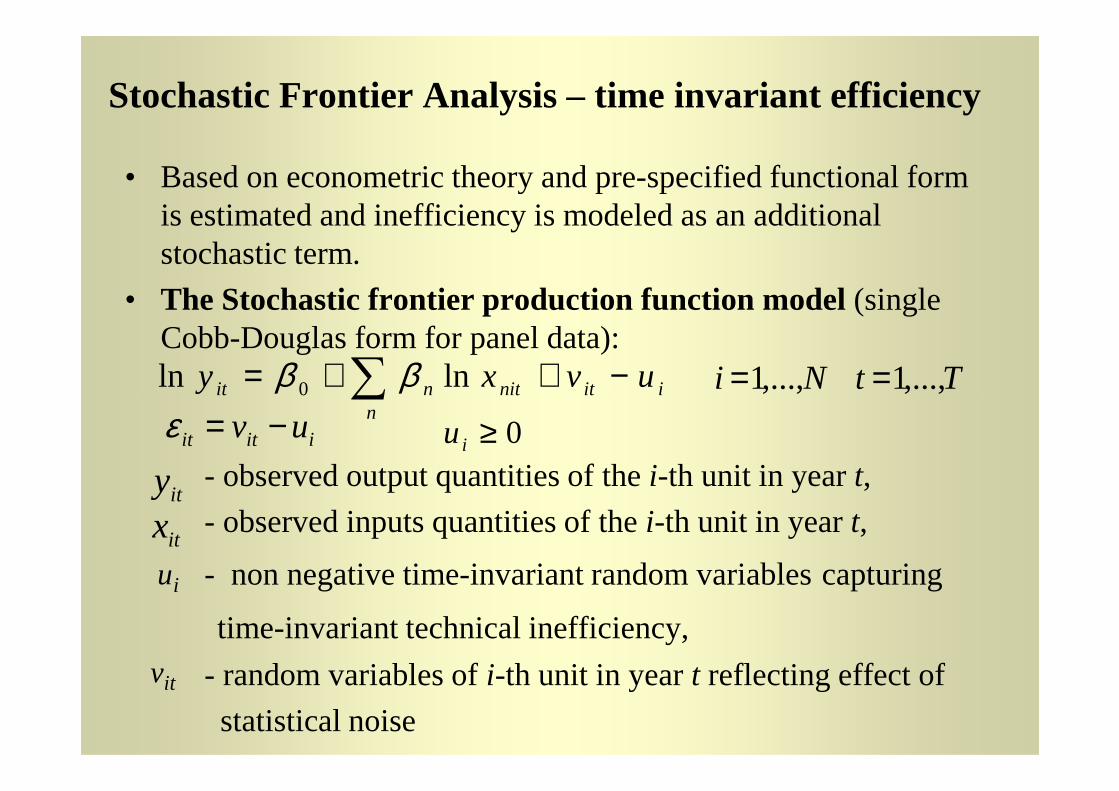
• Based on econometric theory and pre-specified functional form is estimated and inefficiency is modeled as an additional stochastic term.

• The Stochastic frontier production function model(single Cobb-Douglas form for panel data):

Stochastic Frontier Analysis – time invariant efficiency

TtNi ,...,1,...,1 ==iitnitnit uvxy −++= ∑ lnln 0 ββ

- observed output quantities of the i-th unit in year t,

- observed inputs quantities of the i-th unit in year t,

- non negative time-invariant random variables capturing

time-invariant technical inefficiency,

- random variables of i-th unit in year t reflecting effect of

statistical noise

0≥iu

iu

itv

ity

itx

TtNi ,...,1,...,1 ==

iitit uv −=εiit

nnitnit ∑0

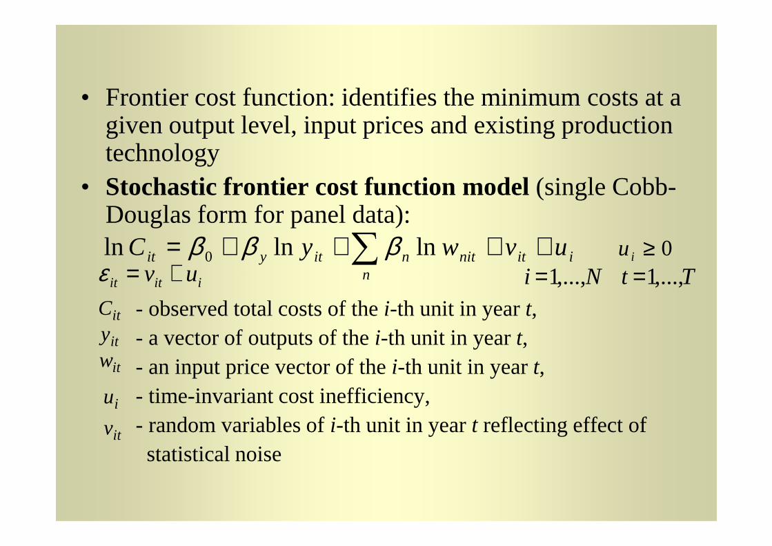
• Frontier cost function: identifies the minimum costs at a given output level, input prices and existing production technology

• Stochastic frontier cost function model(single Cobb-Douglas form for panel data):

iitn

nitnityit uvwyC ++++= ∑ lnlnln 0 βββ 0≥iuTtNi ,...,1,...,1 ==uv +=ε

- observed total costs of the i-th unit in year t,- a vector of outputs of the i-th unit in year t,- an input price vector of the i-th unit in year t,- time-invariant cost inefficiency,- random variables of i-th unit in year t reflecting effect of statistical noise

n

iu

itv

itC

ity

itw

TtNi ,...,1,...,1 ==iitit uv +=ε

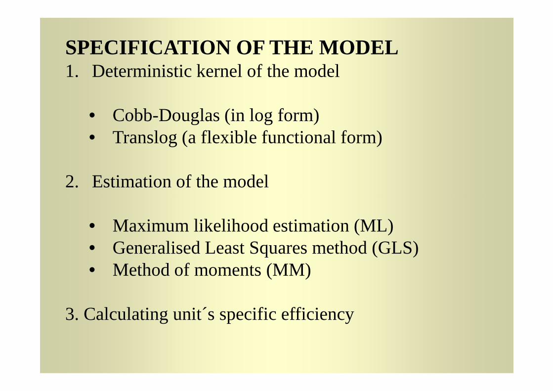
SPECIFICATION OF THE MODEL1. Deterministic kernel of the model

• Cobb-Douglas (in log form)• Translog (a flexible functional form)

2. Estimation of the model

• Maximum likelihood estimation (ML)• Generalised Least Squares method (GLS)• Method of moments (MM)

3. Calculating unit´s specific efficiency

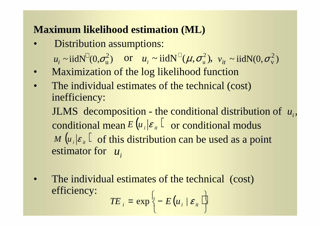
Maximum likelihood estimation (ML)• Distribution assumptions:

or ,• Maximization of the log likelihood function• The individual estimates of the technical (cost)

inefficiency: JLMS decomposition - the conditional distribution of ,

)(0,iidN ~ 2uσ+

iu )iidN(0, ~ 2vσitv

iu

),(iidN ~ 2uσµ+

iu

JLMS decomposition - the conditional distribution of ,conditional mean or conditional modus

of this distribution can be used as a point estimator for

• The individual estimates of the technical (cost) efficiency:

iu( )itiuE ε

( )itiuM ε

iu

( )

−= itii uETE ε|exp

Analyzing Efficiency Behavior

Two questions:

• What is the behavior of efficiencies overtime? Are they increasing, decreasing orconstant?constant?

• What explains the variations in inefficiencies among units and across time?

Time behavior of inefficienciesAssumption:

Model:

tiit uu β+=

TtNi ,...,1,...,1 ==ititnitntit uvxy −++= ∑ lnln 0 ββ

• Cornwell, Schmidt and Sickles, Lee and Schmidt,Kumbhakar, Battese and Coelli

TtNi ,...,1,...,1 ==ititn

nitntit uvxy −++= ∑ lnln 0 ββ

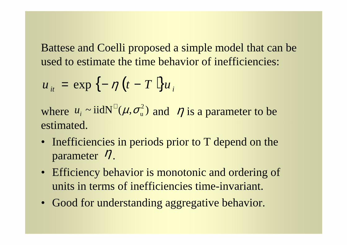
Battese and Coelli proposed a simple model that can be used to estimate the time behavior of inefficiencies:

where and is a parameter to be estimated.

( ){ } iit uTtu −−= ηexp

),(iidN ~ 2uσµ+

iu ηestimated.

• Inefficiencies in periods prior to T depend on the parameter .

• Efficiency behavior is monotonic and ordering of units in terms of inefficiencies time-invariant.

• Good for understanding aggregative behavior.

η

Explaining efficiency

Certain factors influence the environment in whichproduction takes place e.g. degree of competitiveness,input and output quality, network characteristics,ownership form, regulation etc.

Two ways to handle them

• Includethemasvariablesin theproductionprocessas• Includethemasvariablesin theproductionprocessascontrol variables. Using this interpretation, thesevariables influence the structure of the technology bywhich conventional inputs are converted into outputs,but not efficiency.

• Associate variation in estimated efficiency withvariation in the exogenous variables.

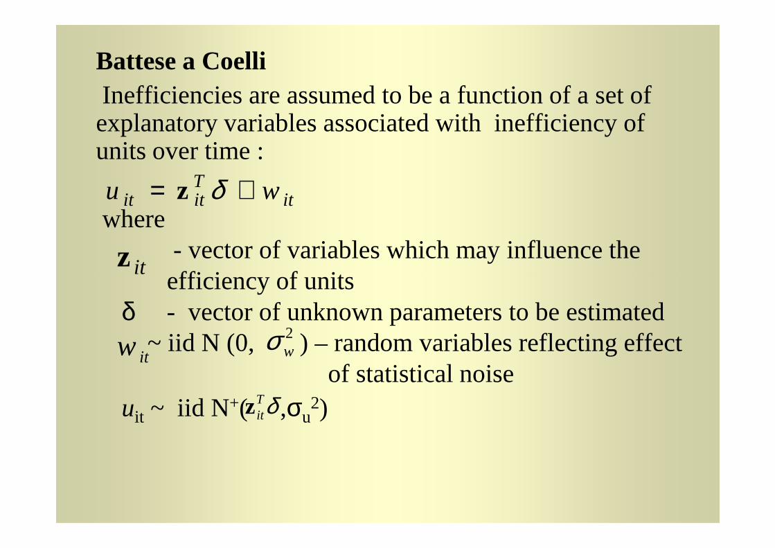
Battese a CoelliInefficiencies are assumed to be a function of a set of explanatory variables associated with inefficiency of units over time :

where - vector of variables which may influence theefficiency of units

itTitit wu += δz

itzefficiency of units

δ - vector of unknown parameters to be estimated~ iid N (0, ) – randomvariables reflecting effect

of statistical noiseuit ~ iid N+( ,σu

2)

it

itw

δTitz

2wσ

EMPIRICAL APPLICATIONS

1. REGULATION OF DISTRIBUTION UTILITIES• Benchmarking analysis can be used by regulator as an

additional instrument to establish a larger informational basis for more effective price cap regulation

• Incentive price–cap regulation ( X – efficiency factor)

Regulation of Slovak and Czech electricity distribution utilities

� Based on incentive price - cap regulation� Main issue: How to set efficiency factor X, i.e. cost

efficiency prediction

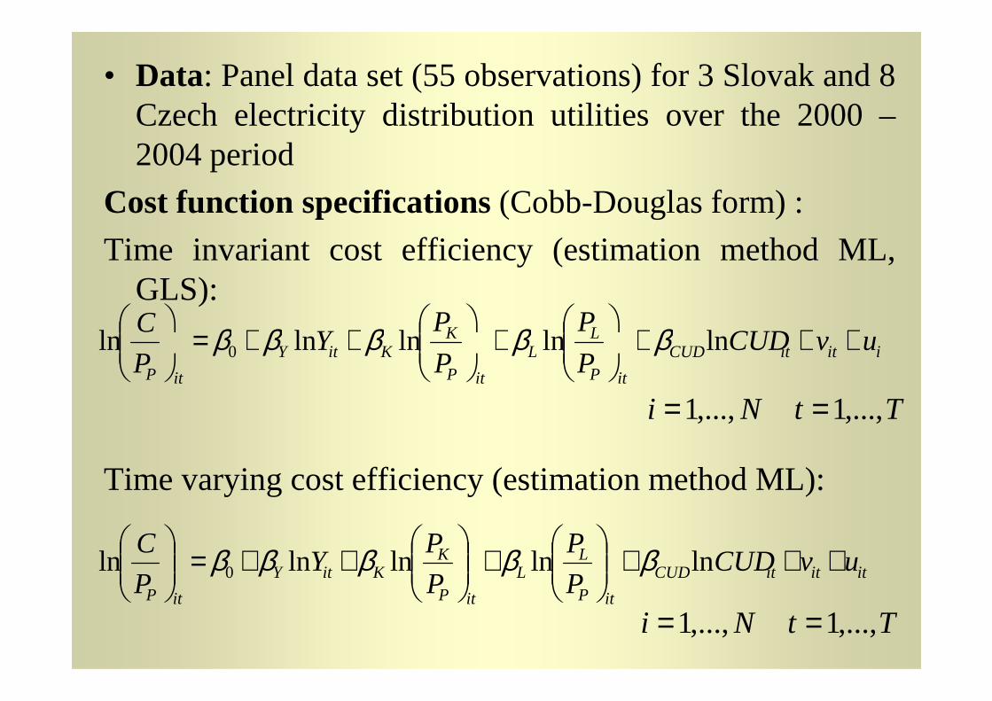
• Data: Panel data set (55 observations) for 3 Slovak and 8Czech electricity distribution utilities over the 2000 –2004 period

Cost function specifications(Cobb-Douglas form) :

Time invariant cost efficiency (estimation method ML,GLS):

iititCUDL

LK

KitY uvCUDP

P

P

PY

P

C +++

+

++=

lnlnlnlnln 0 βββββ

Time varying cost efficiency (estimation method ML):

iititCUD

itPL

itPKitY

itP

uvCUDPP

YP

+++

+

++=

lnlnlnlnln 0 βββββ

itititCUD

itP

LL

itP

KKitY

itP

uvCUDP

P

P

PY

P

C +++

+

++=

lnlnlnlnln 0 βββββ

TtNi ,...,1,...,1 ==

TtNi ,...,1,...,1 ==

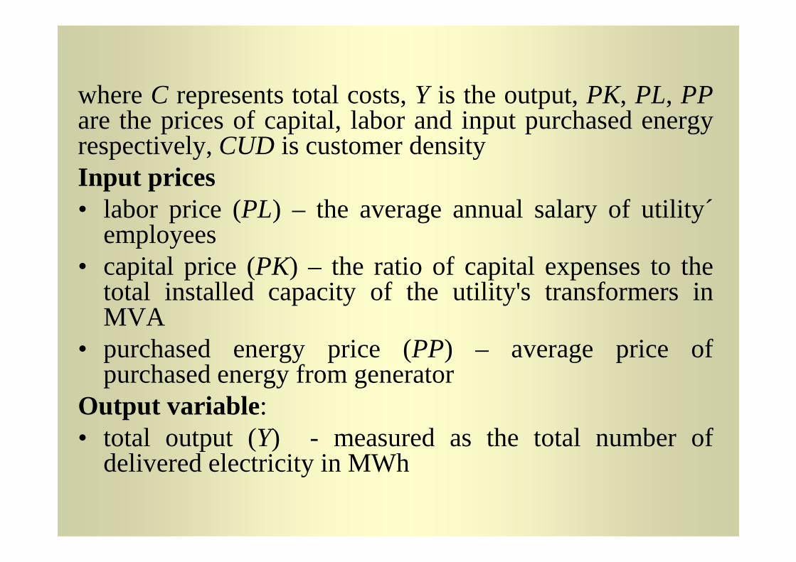
whereC represents total costs,Y is the output,PK, PL, PPare the prices of capital, labor and input purchased energyrespectively,CUD is customer densityInput prices• labor price (PL) – the average annual salary of utility´

employees• capital price (PK) – the ratio of capital expenses to the

total installed capacity of the utility's transformersintotal installed capacity of the utility's transformersinMVA

• purchased energy price (PP) – average price ofpurchased energy fromgenerator

Output variable :• total output (Y) - measured as the total number of

delivered electricity in MWh

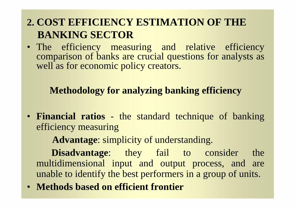
2. COST EFFICIENCY ESTIMATION OF THEBANKING SECTOR

• The efficiency measuring and relative efficiencycomparison of banks are crucial questions for analysts aswell as for economic policy creators.

Methodology for analyzing banking efficiency

• Financial ratios - the standard technique of bankingefficiency measuring

Advantage: simplicity of understanding.Disadvantage: they fail to consider the

multidimensional input and output process, and areunable to identify the best performers in a group of units.

• Methods based on efficient frontier

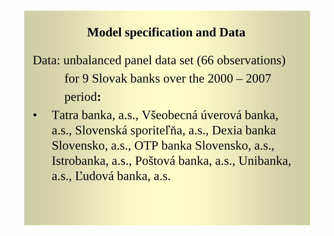
Model specification and Data

Data: unbalanced panel data set (66 observations)

for 9 Slovak banks over the 2000 – 2007

period: • Tatra banka, a.s., Všeobecná úverová banka, • Tatra banka, a.s., Všeobecná úverová banka,

a.s., Slovenská sporiteľňa, a.s., Dexia banka Slovensko, a.s., OTP banka Slovensko, a.s., Istrobanka, a.s., Poštová banka, a.s., Unibanka, a.s., Ľudová banka, a.s.

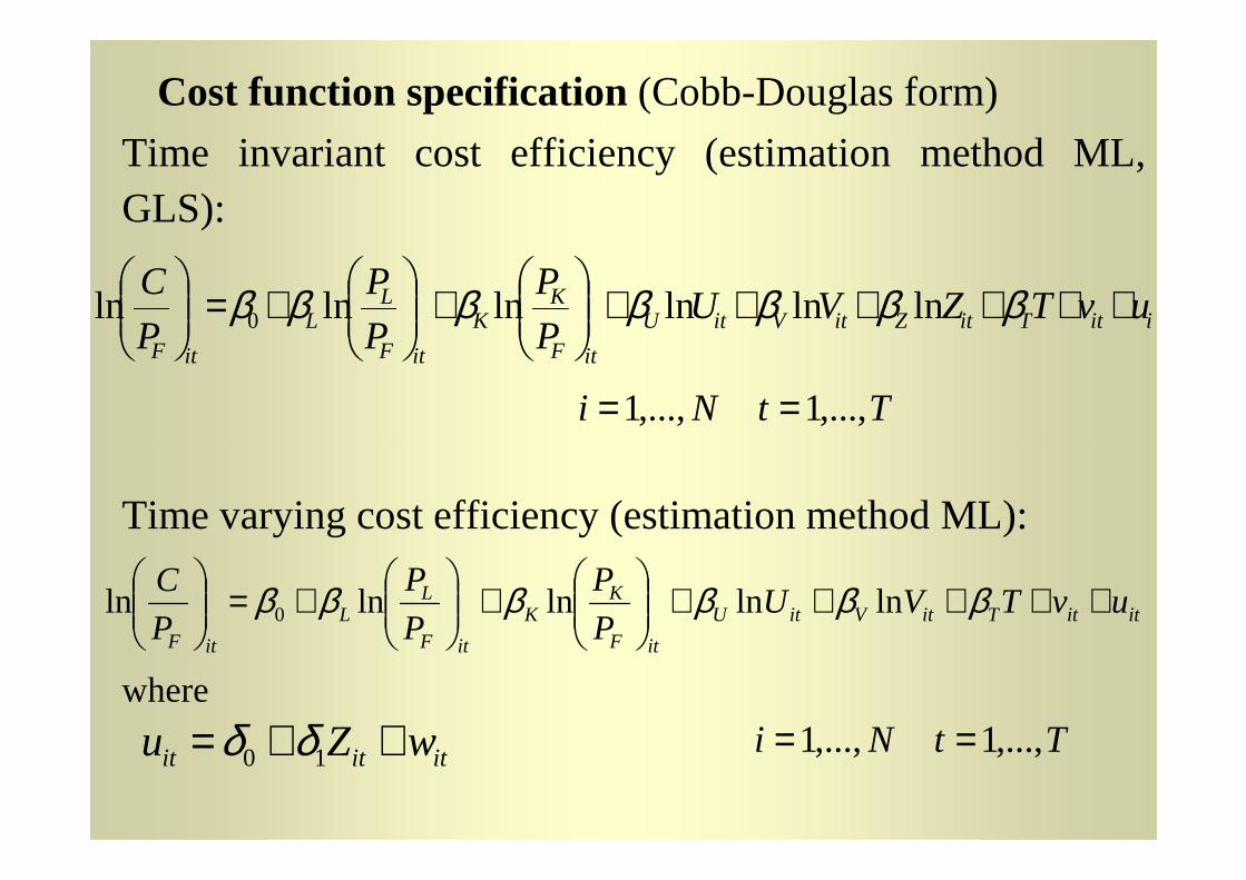
Cost function specification(Cobb-Douglas form)

Time invariant cost efficiency (estimation method ML,GLS):

TtNi ,...,1,...,1 ==

iitTitZitVitU

itF

KK

itF

LL

itF

uvTZVUP

P

P

P

P

C ++++++

+

+=

βββββββ lnlnlnlnlnln 0

Time varying cost efficiency (estimation method ML):

where

TtNi ,...,1,...,1 ==

ititTitVitU

itF

KK

itF

LL

itF

uvTVUP

P

P

P

P

C +++++

+

+=

ββββββ lnlnlnlnln 0

ititit wZu ++= 10 δδ

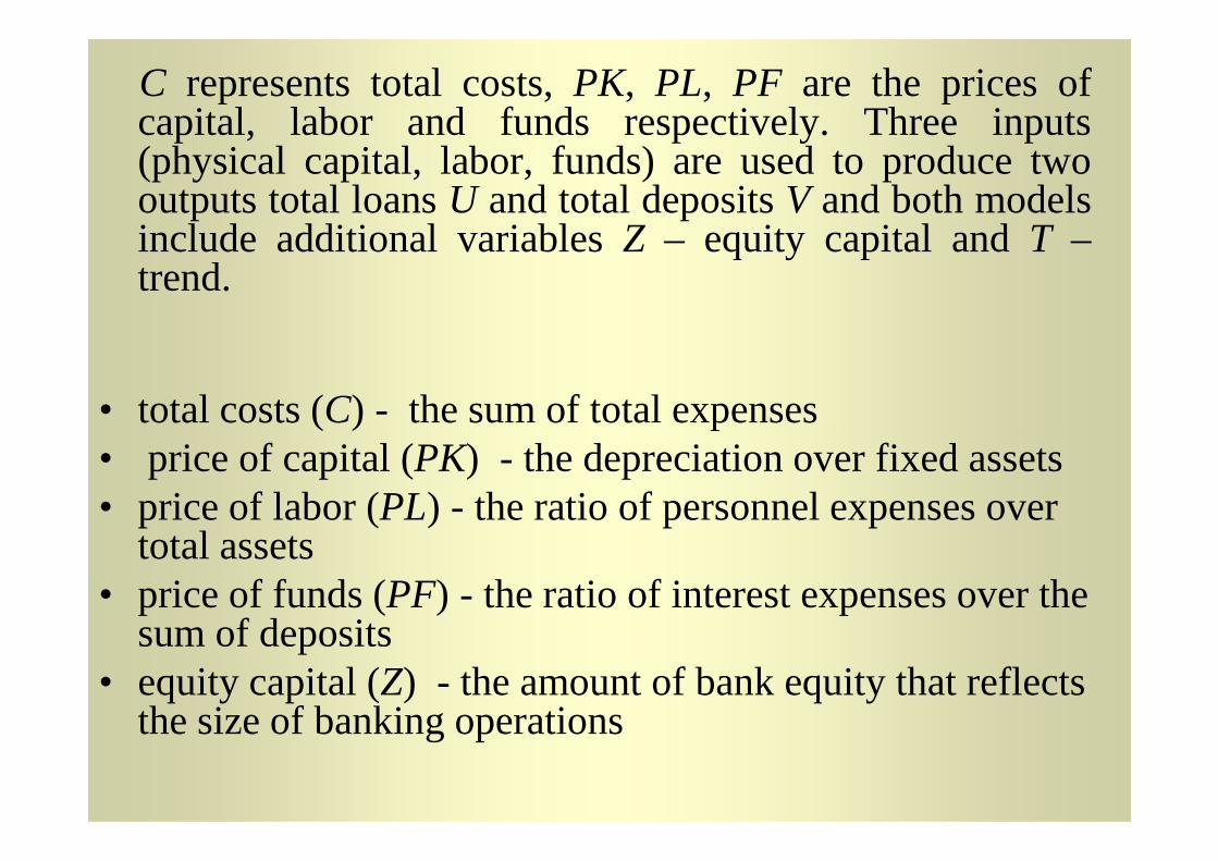
C represents total costs,PK, PL, PF are the prices ofcapital, labor and funds respectively. Three inputs(physical capital, labor, funds) are used to produce twooutputs total loansU and total depositsV and both modelsinclude additional variablesZ – equity capital andT –trend.

• total costs (C) - the sum of total expenses• total costs (C) - the sum of total expenses• price of capital (PK) - the depreciation over fixed assets• price of labor (PL) - the ratio of personnel expenses over

total assets• price of funds (PF) - the ratio of interest expenses over the

sum of deposits• equity capital (Z) - the amount of bank equity that reflects

the size of banking operations

3. ANALYSIS OF REGIONAL COMPETITIVENESS

• Last few years economic policy making and researchhave shown increasing interest for regionalcompetitiveness evaluation (economic efficiency ofregions represents the basis of economic success formicro-economic level and also the competitiveness ofthe country)

Regional competitiveness evaluation methods:Regional competitiveness evaluation methods:Non existence of unique methodology for competitiveness evaluation

• Specific economic indicators of efficiencyIndicator compares a concrete level of the value in the region with respect to its total level in the country

• Methods based on efficient frontier

Model specification and DataThe competitiveness of regions is compared through theestimated levels of technical efficiency as the efficiencyweperceived as the “mirror” of the competitiveness.

Data: balanced panel data set (280 observations)

for 35 V4 (Visegrad four countries) NUTS2(Nomenclature of Units for Territorial Statistics)(Nomenclature of Units for Territorial Statistics)regions observed over a period from 2001 to 2008 :

Slovakia - 4 NUTS2 regions

Czech Republic - 8 NUTS2 regions

Hungary - 7 NUTS2 regions

Poland -16 NUTS2 regions

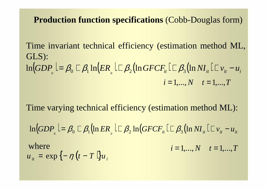
Production function specifications(Cobb-Douglas form)

Time invariant technical efficiency (estimation method ML,GLS):

( ) ( ) ( ) ( ) iititit uvNIGFCFERGDPitit

−++++= lnlnlnln 3210 ββββTtNi ,...,1,...,1 ==

Time varying technical efficiency (estimation method ML):

where

( ) ( ) ( ) ( ) itititit uvNIGFCFERGDPitit

−++++= lnlnlnln 3210 ββββ

( ){ } iit uTtu −−= ηexpTtNi ,...,1,...,1 ==

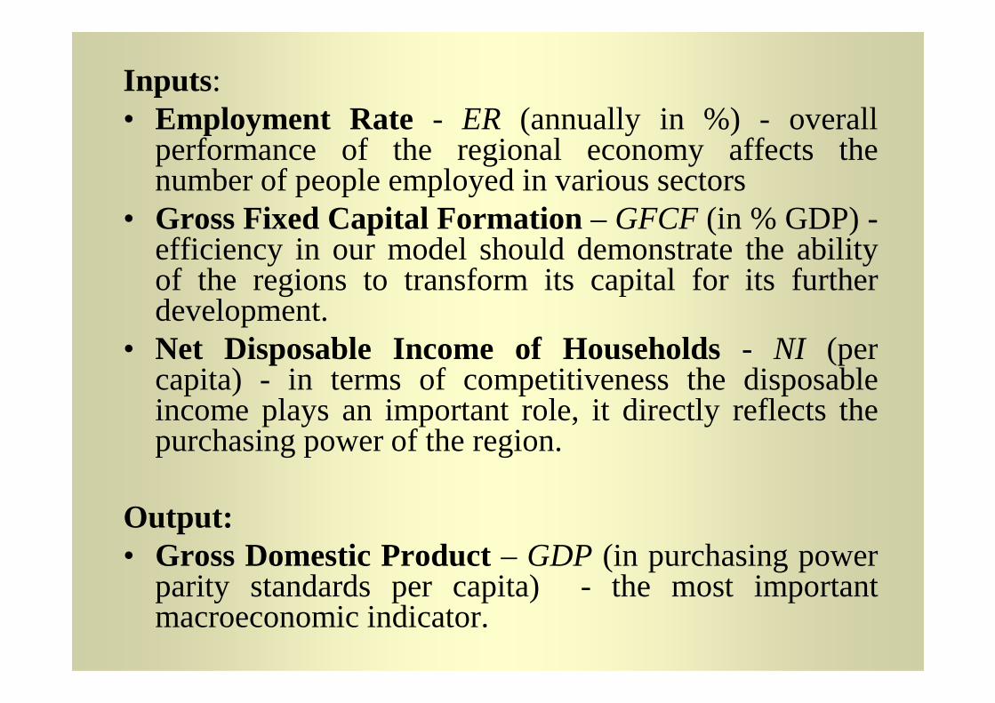
Inputs:• Employment Rate - ER (annually in %) - overall

performance of the regional economy affects thenumber of people employed in various sectors

• Gross Fixed Capital Formation – GFCF (in % GDP) -efficiency in our model should demonstrate the abilityof the regions to transformits capital for its furtherdevelopment.

• Net Disposable Income of Households - NI (per• Net Disposable Income of Households - NI (percapita) - in terms of competitiveness the disposableincome plays an important role, it directly reflects thepurchasing power of the region.

Output:• Gross Domestic Product– GDP (in purchasing power

parity standards per capita) - the most importantmacroeconomic indicator.

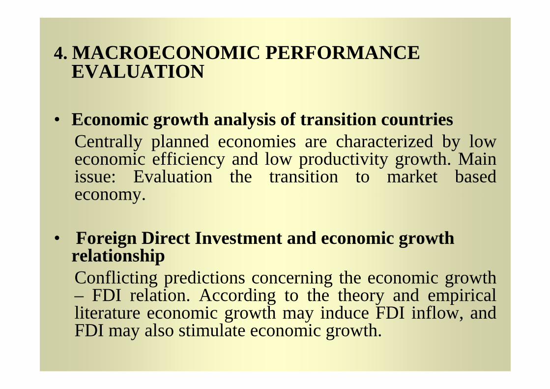
4. MACROECONOMIC PERFORMANCE EVALUATION

• Economic growth analysis of transition countriesCentrally planned economies are characterized by loweconomic efficiency and lowproductivity growth. Mainissue: Evaluation the transition to market basedeconomy.economy.

• Foreign Direct Investment and economic growth relationshipConflicting predictions concerning the economic growth– FDI relation. According to the theory and empiricalliterature economic growth may induce FDI inflow, andFDI may also stimulate economic growth.

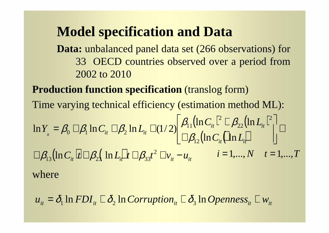
Model specificationand DataData: unbalanced panel data set (266 observations) for

33 OECDcountries observed over a period from2002 to 2010

Production function specification (translog form)

Time varying technical efficiency (estimation methodML):

( ) ( )LC + 22 lnln ββ

where

( ) ( )( )( )

( ) ( ) itititit

itit

itititit

uvttLtC

LC

LCLCY

it

−++++

+

++

+++=

2332313

12

222

211

210

lnln

lnln

lnln)2/1(lnlnln

βββ

ββββββ

ititititit wOpennessCorruptionFDIu +++= lnlnln 321 δδδ

TtNi ,...,1,...,1 ==

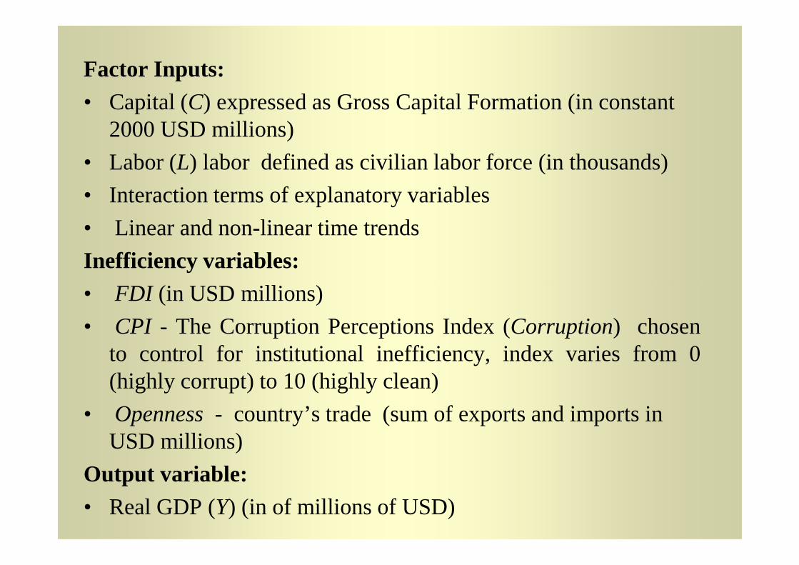
Factor Inputs:• Capital (C) expressed as Gross Capital Formation (in constant

2000 USD millions)

• Labor (L) labor defined as civilian labor force (in thousands)

• Interaction terms of explanatory variables

• Linear and non-linear time trends

Inefficiency variables:• FDI (in USD millions)• FDI (in USD millions)

• CPI - The Corruption Perceptions Index (Corruption) chosento control for institutional inefficiency, index varies from0(highly corrupt) to 10 (highly clean)

• Openness - country’s trade (sum of exports and imports in USD millions)

Output variable:• Real GDP (Y) (in of millions of USD)

USEFULNESS OF SFA• SFAproduces efficiency estimates or efficiency scores

of individual units. Thus one can identify those whoneed intervention and corrective measures.

• SFA provides a powerful tool for examining effects ofintervention. For example, has efficiency of the bankschangedafter deregulation?Has this changevariedchangedafter deregulation?Has this changevariedacross ownership groups?

• Since efficiency scores vary across units, they can berelated to unit´s characteristics like size, ownership,location, etc. Thus one can identify source ofinefficiency.