spatio-temporal point processes: methods and applicationsevents which occur within a pre-speci ed...

Johns Hopkins University, Dept. of Biostatistics Working Papers

6-27-2005

Spatio-temporal Point Processes: Methods andApplicationsPeter J. DiggleMedical Statistics Unit, Lancaster University, UK & Department of Biostatistics, Johns Hopkins Bloomberg School of PublicHealth, [email protected]

This working paper is hosted by The Berkeley Electronic Press (bepress) and may not be commercially reproduced without the permission of thecopyright holder.Copyright © 2011 by the authors

Suggested CitationDiggle, Peter J., "Spatio-temporal Point Processes: Methods and Applications" ( June 2005). Johns Hopkins University, Dept. ofBiostatistics Working Papers. Working Paper 78.http://biostats.bepress.com/jhubiostat/paper78

http://biostats.bepress.com/jhubiostat

Spatio-temporal Point Processes: Methods and

Applications

Peter J Diggle(Department of Mathematics and Statistics, Lancaster University

andDepartment of Biostatistics, Johns Hopkins University School of Public Health)

June 27, 2005

1 Introduction

This chapter is concerned with the analysis of data whose basic format is (xi, ti) : i =1, ..., n where each xi denotes the location and ti the corresponding time of occurrenceof an event of interest. We shall assume that the data form a complete record of allevents which occur within a pre-specified spatial region A and a pre-specified time-interval, (0, T ). We call a data-set of this kind a spatio-temporal point pattern, andthe underlying stochastic model for the data a spatio-temporal point process.

1.1 Motivating examples

1.1.1 Amacrine cells in the retina of a rabbit

One general approach to analysing spatio-temporal point process data is to extendexisting methods for purely spatial data by considering the time of occurrence as adistinguishing feature, or mark, attached to each event. Before giving an examnpleof this, we give an even simpler example of a marked spatial point pattern, in whichthe events are of just two qualitatively different types. Each event in Figure 1 rep-resents the location of an amacrine cell in the retina of a rabbit. These cells play afundamental role in mammalian vision. One type transmits information when a lightgoes on, the other type similarly transmits information when a light goes off. Thedata consist of the locations of 152 on cells and 142 off cells in a rectangular regionof dimension 1060 by 662 µm.

The primary goal for the analysis of these data is to discriminate between two compet-ing developmental hypotheses. The first hypothesis is that the pattern forms initially

1

Hosted by The Berkeley Electronic Press

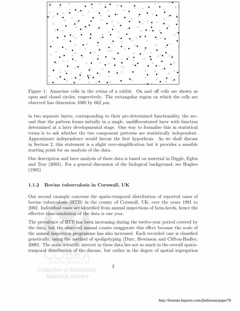
Figure 1: Amacrine cells in the retina of a rabbit. On and off cells are shown asopen and closed circles, respectively. The rectangular region on which the cells areobserved has dimension 1060 by 662 µm.

in two separate layers, corresponding to their pre-determined functionality, the sec-ond that the pattern forms initially in a single, undifferentiated layer with functiondetermined at a later developmental stage. One way to formalise this in statisticalterms is to ask whether the two component patterns are statistically independent.Approximate independence would favour the first hypothesis. As we shall discussin Section 2, this statement is a slight over-simplification but it provides a sensiblestarting point for an analysis of the data.

Our description and later analysis of these data is based on material in Diggle, Eglenand Troy (2005). For a general discussion of the biological background, see Hughes(1985)

1.1.2 Bovine tuberculosis in Cornwall, UK

Our second example concerns the spatio-temporal distribution of reported cases ofbovine tuberculosis (BTB) in the county of Cornwall, UK, over the years 1991 to2002. Individual cases are identified from annual inspections of farm-herds, hence theeffective time-resolution of the data is one year.

The prevalence of BTB has been increasing during the twelve-year period covered bythe data, but the observed annual counts exaggerate this effect because the scale ofthe annual inspection programme has also increased. Each recorded case is classifiedgenetically, using the method of spoligotyping (Durr, Hewinson and Clifton-Hadley,2000). The main scientific interest in these data lies not so much in the overall spatio-temporal distribution of the disease, but rather in the degree of spatial segregation

2

http://biostats.bepress.com/jhubiostat/paper78

140000 160000 180000 200000 220000 240000

2000

040

000

6000

080

000

1000

0012

0000

PSfrag replacements

spoligotype 9

spoligotype 12spoligotype 15spoligotype 20

140000 160000 180000 200000 220000 240000

2000

040

000

6000

080

000

1000

0012

0000

PSfrag replacements

spoligotype 9

spoligotype 12

spoligotype 15spoligotype 20

140000 160000 180000 200000 220000 240000

2000

040

000

6000

080

000

1000

0012

0000

PSfrag replacements

spoligotype 9spoligotype 12

spoligotype 15spoligotype 20140000 160000 180000 200000 220000 240000

2000

040

000

6000

080

000

1000

0012

0000

PSfrag replacements

spoligotype 9spoligotype 12spoligotype 15

spoligotype 20

Figure 2: Spatial distributions of the four most common spoligotype data over thefourteen years.

amongst the different spoligotypes, and whether this spatial segregation is or is notstable over time. If the predominant mode of transmission is through local cross-infection, we might expect to find a stable pattern of spatial segregation, in whichlocally predominant spoligotypes persist over time, whereas if the disease is spreadprimarily by the introduction of animals from remote locations which are bought andsold at market, the resulting pattern of spatial segregation should be less stable overtime (Diggle, Zheng and Durr, 2005).

Figure 2 shows the spatial distributions of cases corresponding to each of the four mostcommon spoligotypes. The visual impression is one of strong spatial segregation, witheach of the four types predominating in particular sub-regions.

3


420000 440000 460000 480000

1000

0012

0000

1400

0016

0000

Figure 3: Locations of 7167 incident cases of non-specific gastroenteric disease inHampshire, 1 January 2001 to 31 December 2002.

1.1.3 Gastroenteric disease in Hampshire, UK

Our third example concerns the spatio-temporal distribution of gastroenteric diseasein the county of Hampshire, UK, over the years 2001 and 2002. The data are derivedfrom calls to NHS Direct, a 24-hour, 7-day phone-in service operating within the UK’sNational Health Service. Each call to NHS Direct generates a data-record whichincludes the caller’s post-code, the date of the call and a symptom code (Cooper,Smith, O’Brien, Hollyoak and Baker, 2003). Figure 3 shows the locations of the 7167calls from patients resident in Hampshire whose assigned symptom code correspondedto acute, non-specific gastroenteric disease. The spatial distribution of cases largelyreflects that of the population of Hampshire, with strong concentrations in the largecities of Southampton and Portsmouth, and smaller concentrations in other towns andvillages. Inspection of a dynamic display of the space-time coordinates of the casessuggests the kind of pattern typical of an endemic disease, in which cases can occurat any point in the study region at any time during the two-year period. Occasionaloutbreaks of gastroenteric disease, which arise as a result of multiple infections froma common source, should result in anomalous, spatially and temporally localisedconcentrations of cases.

The data were collected as part of the AEGISS project (Diggle, Knorr-Held, Rowling-

4


son, Su, Hawtin and Bryant, 2003), whose overall aim was to improve the timelinessof the disease surveillance systems currently used in the UK. The specific statisti-cal aims for the analysis of the data are to establish the normal pattern of spatialand temporal variation in the distribution of reported cases, and hence to developa method of real-time surveillance to identify as quickly as possible any anomalousincidence patterns which might signal the onset of an outbreak requiring some formof public health intervention.

1.1.4 The UK 2001 epidemic of foot-and-mouth disease

Foot-and-mouth disease (FMD) is a highly infectious viral disease of farm livestock.The virus can be spread directly between animals over short distances in contaminatedairborne droplets, and indirectly over longer distances, for example via the movementof contaminated material. The UK experienced a major FMD epidemic in 2001,which resulted in the slaughter of more than 6 million animals. Its estimated totalcost to the UK economy was around £8 billion (UK National Audit Office, 2002).The epidemic affected 44 counties, and was particularly severe in the counties ofCumbria, in the north-west of England, and Devon, in the south-west. Figure 4shows the spatial distributions of all farms in Cumbria and Devon which were at-risk at the start of the epidemic, and of the farms which experienced the disease.In sharp contrast to the data on gastroenteric disease in Hampshire, the case-farmsare strongly concentrated in sub-regions within each of the two counties. Dynamicplotting of the space-time locations of case-farms confirms the typical pattern ofa highly infectious, epidemic disease. The predominant pattern is of transmissionbetween near-neighbouring farms, but there are also a few, apparently spontaneousoutbreaks of the disease far from any previously infected farms.

The main control strategies used during the epidemic involved the pre-emptive slaugh-ter of animal-holdings at farms thought to be at high risk of acquiring, and subse-quently spreading, the disease. Factors which could affect whether a farm is at highrisk include, most obviously, its proximity to infected farms, but also recorded char-acteristics such as the size and species composition of its holding. One objective inanalysing these data is to formulate and fit a model for the dynamics of the diseasewhich incorporates these effects. A model of this kind could then provide informationon what forms of control strategy would be likely to prove effective in any futureepidemic.

1.2 Chapter outline

In Section 2, we give a brief review of statistical methods for spatial point patterns,illustrated by an analysis of the amacrine cell data shown in Figure 1. We referthe reader to Diggle (2003) or Moller and Waagepetersen (2004) for more detailedaccounts of the methodology, and to Diggle, Eglen and Troy (2005) for a full accountof the data-analysis.

5


280000 320000 360000 400000

4600

0050

0000

5400

0058

0000

Easting

Nor

thin

g

200000 250000 300000 350000

5000

010

0000

1500

00

Easting

Nor

thin

g

Figure 4: Locations of at-risk farms (black) and FMD-case farms (red) in Cumbria(left-hand panel) and in Devon (right-hand panel).

In Section 3, we discuss strategies for analysing spatio-temporal point process data.We argue that an important distinction in practice is between data for which theindividual events (xi, ti) occur in a space-time continuum, and data for which thetime-scale is either naturally discrete, or is made so by recording only the aggregatespatial pattern of events over a sequence of discrete time-periods. Our motivatingexamples include instances of each of these scenarios. Other scenarios which we donot consider further are when the locations are coarsely discretised by assigning eachevent to one of a number of sub-regions which form a partition of A. Methods for theanalysis of spatially discrete data are typically based on Markov random field models.An early, classic reference is Besag (1974). Book-length treatments include Cressie(1991), Banerjee, Carlin and Gelfand (2003) and Rue and Held (2005).

In later sections, we describe some of the available models and methods through theirapplication to our motivating examples. This emphasis on specific examples is tosome extent a reflection of the author’s opinion that generic methods for analysingspatio-temporal data-sets have not yet become well-established; certainly, they areless well established than is the case for purely spatial data. Nevertheless, in thefinal section of the chapter we will attempt to draw some general conclusions whichgo beyond the specific examples considered, and can in that sense be regarded aspointers towards an emerging general methodology.

6


2 Statistical methods for spatial point processes

2.1 Descriptors of pattern: spatial regularity, complete spa-

tial randomness and spatial aggregation

A convenient, and conventional, starting point for the analysis of a spatial pointpattern is to apply one or more tests of the hypothesis of complete spatial randomness(CSR), under which the data are a realisation of a homogeneous Poisson process. Ahomogeneous Poisson process is a point process which satisfies two conditions: thenumber of events in any planar region A follows a Poisson distribution with meanλ|A|, where | · | denotes area and the constant λ is the intensity, or mean number ofevents per unit area; and the numbers of events in disjoint regions are independent.It follows that, conditonal on the number of events in any region A, the locationsof the events form an independent random sample from the uniform distribution onA (see, for example, Diggle, 2003, Section 4.4). Hence, CSR embraces two quitedifferent properties: a uniform marginal distribution of events over the region A; andindependence of events. We emphasise that this is only a starting point, and thatthe hypothesis of CSR is rarely of any scientific interest. Rather, CSR is a dividinghypothesis (Cox, 1977), a test of which leads to a qualitative classification of anobserved pattern as regular, approximately random or aggregated.

We do not attempt a precise mathematical definition of the descriptions “regular”and “aggregated.” Roughly speaking, a regular pattern is one in which events aremore evenly spaced throughout A than would be expected under CSR, and typicallyarises through some form of inhibitory dependence between events. Conversely, anaggregated pattern is one in which events tend to occur in closely spaced groups.Patterns of this type can arise as a consequence of marginal non-uniformity or a formof attractive dependence, or both. In general, as shown by Bartlett (1964), it is notpossible to distinguish empirically between underlying hypotheses of non-uniformityand dependence, using the information presented by a single observed pattern. Figure5 shows an example of a regular, a completely random and an aggregated spatial pointpattern. The contrasts amongst the three are clear.

2.2 Functional summary statistics

Tests of CSR which are constructed from functional summary statistics of an observedpattern are useful for two reasons: when CSR is conclusively rejected, their behaviourgives clues as to the kind of model which might provide a reasonable fit to the data;and they may suggest preliminary estimates of model parameters. Two widely usedways of constructing functional summaries are through nearest neighbour and second-moment properties. Third and higher-order moment summaries are easily defined,but appear to be rarely (possibly too rarely) used in data-analysis; an exceptionis Peebles and Groth (1975). They do feature more prominently in the theoretical

7


•

•

• ••

•

•

••

•

•

•

•

•

•

••

•

•

•

•

•

•

•

•

•

•

•

•

•

•

•

•

•

•

•

••

••

•

•

•

•

•

••

• •

•

•

•

•

•

•

•

•

•

•

•

••

•

•

•

•

•

••

•

•

•

•

•

••

•

•

•

•

•

•

•

•

•

•••

•

•

•

•

•

•

•

•

•

•

•

•

0.0 0.2 0.4 0.6 0.8 1.0

0.0

0.2

0.4

0.6

0.8

1.0

•

•

•

•

•

•

•

• ••

•

•

•

•

••

•

•

•

• •

•

•

•

•

•

•

•

•

•

•

•

••

•

••

•

•

•

•

•

•

•

•

•

•

•

•

•

•

•

•

•

•

•

•

•

•

•

•

•

•

•

•

••

•

•

•

•

•

•

•

• •

•

•

•

•

•

•

•

•

•

•

•

•

•

•

•

•

•

•

•

•

•

•

•

•

0.0 0.2 0.4 0.6 0.8 1.0

0.0

0.2

0.4

0.6

0.8

1.0

•

•

••

• •••

•

••

•

•

•

•

•

•

•

•

•

•

•

•

•

•

••

•

•

•

•

•

••

••

•

••

• •

•

•

•

•

•

•

•

••

•

•

•

•

•

•

•

••

•

•

• •

•

•

•

•

•

•

•

•

•

•

•

••

•• •

•

•

•

•

•

•

•

•

•

•

•

•

•

•

•

•

•

•

•

•

•

0.0 0.2 0.4 0.6 0.8 1.0

0.0

0.2

0.4

0.6

0.8

1.0

Figure 5: Examples of a regular (upper-left panel), a completely random (upper-rightpanel)and an aggregated (lower panel) spatial point pattern.

analysis of ecological models, as discussed elsewhere in this volume, and undoubtedlyoffer potential insights which are not captured by second-moment properties.

Two nearest neighbour summaries are the distribution functions of X, the distancefrom an arbitrary origin of measurement to the nearest event of the process, and ofY , the distance from an arbitrary event of the process to the nearest other event.We denote these by F (x) and G(y), respectively. The empirical counterpart of F (x)typically uses the distances, di say, from each of m points in a regular lattice arrange-ment to the nearest event, leading to the estimate F (x) = m−1 ∑

I(di ≤ x) whereI(·) is the indicator function. Similarly, if ei is the distance from each of n eventsto its nearest neighbour, then G(y) = n−1 ∑

I(ei ≤ y). Edge-corrected versions ofthese simple estimators are sometimes preferred, and are necessary if we wish to com-pare empirical estimates with the corresponding theoretical properties of a stationarypoint process.

Derivations, and further discussion, of results in the remainder of this Section can befound, for example, in Diggle (2003, Chapter 4).

Under CSR, F (x) = G(x) = 1 − exp(−λπx2), where λ is the intensity, or meannumber of events per unit area. Typically, in a regular pattern G(x) < F (x), whereasin an aggregated pattern G(x) > F (x).

To describe the second-moment properties of a spatial point process, we need some

8


additional notation. Let dx denote an infinitesimal neighbourhood of the point x,and N(dx) the number of events in dx. Then, the intensity function of the process is

λ(x) = lim|dx|→0

{

E[N(dx)]

|dx|

}

.

Similarly, the second-moment intensity function is

λ2(x, y) = lim|dx|→0|dy|→0

{

E[N(dx)N(dy)]

|dx||dy|

}

and the covariance density is

γ(x, y) = λ2(x, y) − λ(x)λ(y).

The process is stationary and isotropic if its statistical properties do not change undertranslation and rotation, respectively. If we now assume that the process is stationaryand isotropic, the intensity function reduces to a constant, λ, equal to the expectednumber of events per unit area. Also, the second-moment intensity reduces to afunction of distance, λ2(x, y) = λ2(r) where r = ||x − y|| is the distance between xand y, and the covariance density is γ(r) = λ2(r)−λ2. In this case, the scaled quantityρ(r) = λ2(r)/λ

2 is called, somewhat misleadingly, the pair correlation function. Fora homogeneous Poisson process, g(r) = 1 for all r.

A more tangible interpretation of the pair correlation function is obtained if we in-tegrate over a disc of radius s. This gives the reduced second-moment measure, orK-function,

K(s) = 2π∫ s

0ρ(r)rdr. (1)

Ripley (1976, 1977) introduced the K-function as a tool for data-analysis. One of itsadvantages over the pair correlation function is that it can be interpreted as a scaledexpectation of an observable quantity. Specifically, let E(s) denote the expectednumber of further events within distance s of an arbitrary event. Then,

K(s) = λ−1E(s). (2)

The result (2) leads to several useful insights. Firstly, it suggests a method of estimat-ing K(s) directly by the method of moments, without the need for any smoothing;this is especially useful for relatively small data-sets. Secondly, it explains why K(s)is a good descriptor of spatial pattern. For a completely random pattern, events arepositioned independently, hence E(s) = λπs2 and K(s) = πs2. This gives a bench-mark against which to assess departures from CSR. For aggregated patterns, K(s)is relatively large at small distances s because each event typically forms part of a“cluster” of mutually close events. Conversely, for regular patterns K(s) is relativelysmall at small distances s because each event tends to be surrounded by empty space.Another useful property is that K(s) is invariant to random thinning, i.e. retentionor deletion of events according to a series of independent Bernoulli trials. This follows

9


s

K(s

)-pi

*s*s

0.0 0.05 0.10 0.15 0.20 0.25

-0.0

20.

00.

020.

04

Poissonclusteredregular

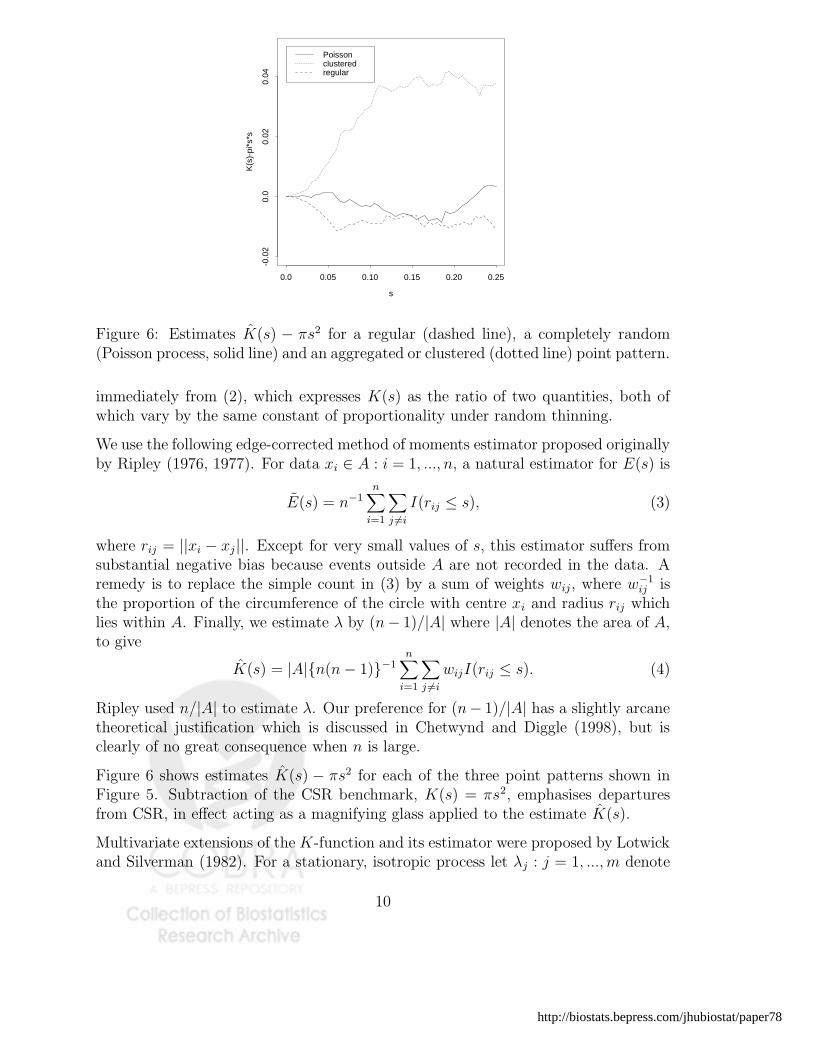
Figure 6: Estimates K(s) − πs2 for a regular (dashed line), a completely random(Poisson process, solid line) and an aggregated or clustered (dotted line) point pattern.

immediately from (2), which expresses K(s) as the ratio of two quantities, both ofwhich vary by the same constant of proportionality under random thinning.

We use the following edge-corrected method of moments estimator proposed originallyby Ripley (1976, 1977). For data xi ∈ A : i = 1, ..., n, a natural estimator for E(s) is

E(s) = n−1n

∑

i=1

∑

j 6=i

I(rij ≤ s), (3)

where rij = ||xi − xj||. Except for very small values of s, this estimator suffers fromsubstantial negative bias because events outside A are not recorded in the data. Aremedy is to replace the simple count in (3) by a sum of weights wij, where w−1

ij isthe proportion of the circumference of the circle with centre xi and radius rij whichlies within A. Finally, we estimate λ by (n− 1)/|A| where |A| denotes the area of A,to give

K(s) = |A|{n(n − 1)}−1n

∑

i=1

∑

j 6=i

wijI(rij ≤ s). (4)

Ripley used n/|A| to estimate λ. Our preference for (n− 1)/|A| has a slightly arcanetheoretical justification which is discussed in Chetwynd and Diggle (1998), but isclearly of no great consequence when n is large.

Figure 6 shows estimates K(s) − πs2 for each of the three point patterns shown inFigure 5. Subtraction of the CSR benchmark, K(s) = πs2, emphasises departuresfrom CSR, in effect acting as a magnifying glass applied to the estimate K(s).

Multivariate extensions of the K-function and its estimator were proposed by Lotwickand Silverman (1982). For a stationary, isotropic process let λj : j = 1, ..., m denote

10


the intensity of type j events. Define functions Kij(s) = λ−1j Eij(s), where Eij(s)

is the expected number of further type j events within distance s of an arbitrarytype i event. Note that Kij(s) = Kji(s). Although this equality is not obviousfrom the above definitions, it follows immediately from the multivariate analogueof our earlier definition (1) of K(s) as an integrated version of the pair correlationfunction. However, direct extension of (4) to the multivariate case leads to twodifferent estimates Kij(s) and Kji(s) which, following Lotwick and Silverman (1982),we can combine to give the single estimate

Kij(s) = {niKij(s) + njKji(s)}/(ni + nj). (5)

Two useful benchmark results for multivariate K-functions are:

(i) if type i and type j events form independent processes, then Kij(s) = πs2;

(ii) if type i and type j events form a random labelling of a univariate process withK-function K(s), then Kii(s) = Kjj(s) = Kij(s) = K(s).

2.3 Functional summary statistics for the amacrines data

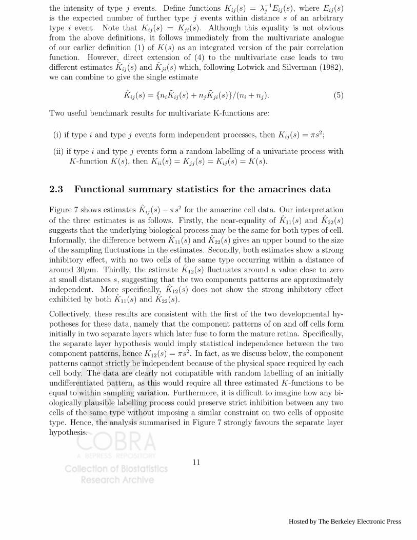
Figure 7 shows estimates Kij(s)− πs2 for the amacrine cell data. Our interpretation

of the three estimates is as follows. Firstly, the near-equality of K11(s) and K22(s)suggests that the underlying biological process may be the same for both types of cell.Informally, the difference between K11(s) and K22(s) gives an upper bound to the sizeof the sampling fluctuations in the estimates. Secondly, both estimates show a stronginhibitory effect, with no two cells of the same type occurring within a distance ofaround 30µm. Thirdly, the estimate K12(s) fluctuates around a value close to zeroat small distances s, suggesting that the two components patterns are approximatelyindependent. More specifically, K12(s) does not show the strong inhibitory effectexhibited by both K11(s) and K22(s).

Collectively, these results are consistent with the first of the two developmental hy-potheses for these data, namely that the component patterns of on and off cells forminitially in two separate layers which later fuse to form the mature retina. Specifically,the separate layer hypothesis would imply statistical independence between the twocomponent patterns, hence K12(s) = πs2. In fact, as we discuss below, the componentpatterns cannot strictly be independent because of the physical space required by eachcell body. The data are clearly not compatible with random labelling of an initiallyundifferentiated pattern, as this would require all three estimated K-functions to beequal to within sampling variation. Furthermore, it is difficult to imagine how any bi-ologically plausible labelling process could preserve strict inhibition between any twocells of the same type without imposing a similar constraint on two cells of oppositetype. Hence, the analysis summarised in Figure 7 strongly favours the separate layerhypothesis.

11


0 50 100 150

−60

00−

4000

−20

000

2000

PSfrag

replacem

ents

s

K(s

)−

πs2

Figure 7: Estimates of the K-functions for the amacrine cell data. Each plottedfunction is K(s) − πs2. The dashed line corresponds to K11(s) (on cells), the dottedline to K22(s) (off cells) and the solid line to K12(s). The parabola −πs2 is also shownas a solid line.

2.4 Likelihood-based methods

Classical maximum likelihood estimation is straightforward for Poisson processes, butnotoriously intractable for other point process models. Two more tractable alterna-tives are maximum pseudo-likelihood and Monte Carlo maximum likelihood. Bothare particularly well-suited to estimation in a class of models known as pairwise in-teraction point processes, and it is this context that we discuss them here.

A third variant of likelihood-based estimation uses a partial likelihood. This methodis best known in the context of survival analysis (Cox, 1972, 1975). We describe itsadaptation to spatio-temporal point processes in Section 3.2.2.

2.4.1 Pairwise interaction point processes

Pairwise interaction processes form a sub-class of Markov point processes (Ripley andKelly, 1977). They are defined by their likelihood ratio, f(·), with respect to a Poissonprocess of unit intensity. Hence, if χ = {x1, ..., xn} denotes a configuration of n pointsin a spatial region A, then f(χ) measures in an intuitive sense how much more likelyis the configuration χ than it would be as a realisation of a Poisson process of unitintensity. For a pairwise interaction process, we need to specify a parameter β wichgoverns the mean number of events per unit area and an interaction function h(r),where r denotes distance. Intuitively, h(r) is related to the likelihood that the modelwill generate pairs of events separated by a distance r, in the sense that the likeklihoodfor a particular configuration of events depends on the product of h(||xi − xj||) overall distinct pairs of events. Hence, for example, a value h(r) = 0 for all r < δ would

12


imply that no two events can be separated by a distance less than δ. The likelihoodratio f(χ) for the resulting pairwise interaction point process is

f(χ) = c(β, h)βn∏

j<i

h(||xi − xj||), (6)

where c(β, h) is a normalising constant which is generally intractable. Note that in ahomogeneous Poisson process, the number of points in A follows a Poisson distributionwith mean proportional to |A| and, conditional on the number of points in A, theirlocations form an independent random sample from the uniform distribution on A. Itfollows that a homogeneous Poisson process is a special case of a pairwise interactionprocess in which h(u) = 1 for all u, and β is the intensity. More generally, in (6)the parameter β is related to, but not necessarily equal to, the intensity. Providedthat the specified form of h(·) is legitimate, values of h(r) less than or greater than 1correspond to processes which generate regular or aggregated patterns, respectively.

A sufficient condition for legitimacy is that h(r) ≤ 1 for all r, as this guarantees afinite intensity for the resulting point process. It also leads to point patterns whosecharacter is inhibitory, meaning that close pairs of events are relatively unlikely bycomparison with a Poisson process of the same intensity. Pairwise interaction pointprocess of this kind are widely used for modelling regular spatial point patterns.

Specifications in which h(u) > 1 are more problematic. An intuitive explanationfor this is that if, over a range of distances r, the interaction function takes valuesh(r) ≥ h0, where h0 > 1, then the product term on the right hand side of (6) can

be as large as hn(n−1)/20 , and this cannot be balanced by adjusting the value of β in

(6). Hence, the likelihood increases without limit as n → ∞. This perhaps explainswhy, even if we are prepared to consider n as fixed, pairwise interaction processes withh(r) > 1 tend to generate unrealistically strong spatial aggregation,with large clustersof near-coincident events. For a rigorous discussion of the properties of pairwiseinteraction processes with h(r) > 1, see Gates and Westcott (1986).

2.4.2 Maximum pseudo-likelihood

The method of maximum pseudo-likelihood was originally proposed by Besag (1975,1978) as a method for real-valued, spatially discrete processes. Besag et al (1982)derived a point process version by considering a limit of binary-valued processes ona lattice, as the lattice spacing tends to zero. For a finite-dimensional probabilitydistribution, the pseudo-likelihood is the product of the full conditional distributions,i.e. the conditional distributions of each Yi given the values of all other Yj. Hence, ifY = (Y1, ..., Yn) has joint probability density f(y), then the pseudo-likelihood is, inan obvious notation,

∏ni=1 f(yi|yj, j 6= i).

For a point process, the pseudo-likelihood uses conditional intensities in place ofthe full conditional distributions. In particular, for a Markov point process withlikelihood ratio f(·), the conditional intensity for an arbitrary point u given the

13


observed configuration X on A − {u} is

λ(u; X) =

{

f(X ∪ {u})/f(X) : u /∈ Xf(X)/f(X − {u}) : u ∈ X

and the log-pseudo-likelihood is

n∑

i=1

log λ(xi; X) −∫

Aλ(u; X)du.

2.4.3 Monte Carlo maximum likelihood

Monte Carlo maximum likelihood estimation, as described here, was proposed byGeyer and Thompson (1992). Geyer (1999) and Moller and Waagepetersen (2004)discuss the method in the context of point process models including, but not restrictedto, pairwise interaction point processes.

Conditional on the number of events in a specified region A, the likelihood for apairwise interaction point process can be written in principle as

`(θ) = c(θ)f(X; θ), (7)

where X = {x1, ..., xn} is the observed configuration of the n events in A. For mostmodels of interest, the normalising constant c(θ) in (7) is intractable. However, notethat

c(θ)−1 =∫

Xf(X; θ)dX

=∫

Xf(X; θ) ×

c(θ0)

c(θ0)×

f(X; θ0)

f(X; θ0),

for any value of θ0. If we now define r(X; θ, θ0) = f(X; θ)/f(X; θ0) then we can write

c(θ)−1 = c(θ0)−1

∫

Xr(X; θ, θ0)c(θ0)f(X; θ)dX

= c(θ0)−1Eθ0

[r(X; θ, θ0)]dX,

where Eθ0[·] denotes expectation with respect to the distribution of X when θ = θ0.

This in turn allows us to re-express the likelihood (7) as

`(θ) = c(θ0)f(X; θ)/Eθ0[r(X; θ, θ0)]. (8)

It follows from (8) that for any fixed value θ0, the maximum likelihood estimator θmaximises

Lθ0(θ) = log f(X; θ) − log Eθ0

[r(X; θ, θ0)]. (9)

Now, choose any value θ0, simulate realisations Xj : j = 1, ..., s with θ = θ0 and define

Lθ0,s(θ) = log f(X; θ) − log s−1s

∑

j=1

[r(Xj; θ, θ0)]. (10)

14


Then, the value θMC which maximises (10) is a Monte Carlo maximum likelihoodestimator (MCMLE) for θ. Note the indefinite article. A Monte Carlo log-likelihoodLθ0,s(θ) is typically a smooth function of θ and can easily be maximised numerically,but it is also a function of θ0, s and the simulated realisations Xj. In practice, wewould want to choose s sufficiently large that the Monte Carlo variation introducedby using a sample average in place of the expectation on the right-hand side of (9) isnegligible. However, for given s the behaviour of the MCMLE is critically dependenton the choice of θ0, the ideal being to choose θ0 equal to θ in which case the MonteCarlo variation in (10) is zero at θ = θ. More generally, obtaining a sufficientlyaccurate Monte Carlo approximation to the intractable expectation in (9) raises anumber of practical issues which, in the author’s experience, make it difficult toautomate the procedure.

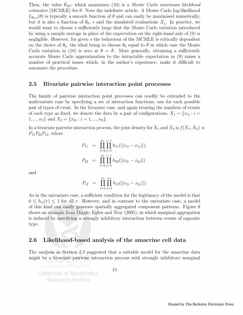
2.5 Bivariate pairwise interaction point processes

The family of pairwise interaction point processes can readily be extended to themultivariate case by specifying a set of interaction functions, one for each possiblepair of types of event. In the bivariate case, and again treating the numbers of eventsof each type as fixed, we denote the data by a pair of configurations, X1 = {x1i : i =1, ..., n1} and X2 = {x2i : i = 1, ..., n2}.

In a bivariate pairwise interaction process, the joint density for X1 and X2 is f(X1, X2) ∝P11P22P12, where

P11 =n1∏

i=2

i−1∏

j=1

h11(||x1i − x1j||),

P22 =n2∏

i=2

i−1∏

j=1

h22(||x2i − x2j||)

and

P12 =n1∏

i=1

n2∏

j=1

h12(||x1i − x2j ||).

As in the univariate case, a sufficient condition for the legitimacy of the model is that0 ≤ hij(r) ≤ 1 for all r. However, and in contrast to the univariate case, a modelof this kind can easily generate spatially aggregated component patterns. Figure 8shows an example from Diggle, Eglen and Troy (2005), in which marginal aggregationis induced by specifying a strongly inhibitory interaction between events of oppositetype.

2.6 Likelihood-based analysis of the amacrine cell data

The analysis in Section 2.3 suggested that a suitable model for the amacrine datamight be a bivariate pairwise interaction process with strongly inhibitory marginal

15


Figure 8: Simulated realisations of bivariate pairwise interaction point processes eachwith 50 events of either type on the unit square and simple inhibitory interactionfunctions. In both panels, the minimum permissible distance between any two eventsof the same type is 0.025. In the left-hand panel, the two component patterns areindependent. In the right-hand panel, the minimum permissible distance betweenany two events of opposite types is 0.1.

properties and approximate independence between the two components.

Our first stage in fitting a model of this kind is to use maximum pseudo-likelihoodestimation in conjunction with a piece-wise constant specification of h(u) to identifya candidate model for the interaction within each component pattern. We then useMonte Carlo maximum likelihood to fit a suitable parametric model to each compo-nent. Figure 9 shows the result, together with a Monte Carlo maximum likelihoodestimate using the parametric model

h(u; θ) =

{

0 : u ≤ δ1 − exp[−{(u − δ)/φ}α] : u > δ

. (11)

The fit adopts common parameter values for the two types of cell, on the basis ofa Monte Carlo likelihood ratio test under the assumption that the two componentprocesses are independent; for details, see Diggle, Eglen and Troy (2005). In fittingthe parametric model, we used a fixed value δ = 10µm, representing the approximatephysical size of each cell body, and estimated the remaining parameters as φ = 49.08and α = 2.92.

For the bivariate analysis, we use the same parametric form (11) for the three inter-action functions h11(r), h22(r) and h12(r). For φ tending to zero, the model for h12(r)reduces to a simple inhibitory form, h12(r) = 0 for r < δ12 and h12(r) = 1 otherwise,with independence of the two components as the special case δ12 = 0. Independenceis strictly impossible because no two cells can occupy the same location, but it isreasonable to treat δ12 as a parameter to be estimated because the two types of cellare located at slightly different depths within the retina. Diggle, Eglen and Troy(2005) conclude that a bivariate model with a simple inhibitory h12(r) and δ12 = 4.9gives a reasonable fit to the data.

16


0 50 100 150 200

0.0

0.2

0.4

0.6

0.8

1.0

1.2

PSfrag

replacem

ents

rh(r

)

Figure 9: Non-parametric maximum pseudo-likelihood estimates of the pairwise in-teraction functions for on cells (solid line) and for off cells (dashed line), togetherwith parametric fit assuming common parameter values for both types of cell (dottedline).

3 Strategies for the analysis of spatio-temporal point

patterns

Many of the tools used to analyse spatial point process data can be extended to thespatio-temporal setting. Functional summaries based on low-order moments can beextended in the obvious way by considering configurations of events at specified spa-tial and temporal positions. For example, Diggle, Chetwynd, Haggkvist and Morris(1995) defined a spatio-temporal K-function K(s, t) such that λK(s, t) is the ex-pected number of further events within distance s and time t of an arbitrary eventof the process. Bhopal, Diggle and Rowlingson (1992) used an estimate of K(s, t) toanalyse the spatio-temporal distribution of apparently sporadic cases of legionnaire’sdisease. However, the spatio-temporal setting opens up other modelling and analysisstrategies which take more explicit account of the directional character of time, andthe consequently richer opportunities for scientific inference.

3.1 Strategies for discrete-time data

As noted earlier, discrete-time spatio-temporal point process data can arise in twoways; either the underlying process genuinely operates in discrete-time, or an un-derlying continuous-time process is observed at a discrete sequence of time-points.A hypothetical example of the former would be the yearly sequence of spatial pointdistributions formed by the natural regeneration of an annual plant community. TheCornwall BTB data described in Section 1.1.2 are an example of the latter.

17


3.1.1 Transition models

For genuinely discrete-time processes, a natural strategy is to build a transition modelto describe the changes between successive times. In symbolic notation, if Pt denotesthe spatial point process at time t a transition model for the joint distribution ofP = {P1,P2, ..,Pt} takes the form

[P] = [P1][P2|P1]...[Pt|Pt−1, ...P1] (12)

A convenient working assumption would be that the process is Markov in time, andthis may have some mechanistic justification when times correspond to successivegenerations, as in our hypothetical example.

3.1.2 A transition model for spatial aggregation

A standard example of a spatial point process model which leads to spatially ag-gregated patterns is a Neyman-Scott clustering process (Neyman and Scott, 1958),defined as follows. Parent events form a homogeneous Poisson process with intensityρ events per unit area. The parents then generate numbers of offspring as an inde-pendent random sample from the Poisson distribution with mean µ. The positionsof the offspring relative to their parents are an independent random sample fromthe bivariate Normal distribution with mean zero and variance matrix σ2I, whereI denotes the identity matrix. The observed point pattern is then taken to be thesuperposition of the offspring from all parents.

An obvious way to turn the Neyman-Scott process into a transition model is to letthe offspring of one generation become the parents for the next generation. Kingman(1977) discusses a model of this kind in questioning whether the basic Neyman-Scottformulation can arise as the equilibrium distribution of a spatio-temporal process.Note in particular that the spatio-temporal process defined in this way may die outafter a finite number of generations. Figure 10 shows the result of a simulation on theunit square with periodic boundary conditions, i.e. events are generated on a torus,which is then unwrapped to form the unit square region A. The model parameters areρ = 100, σ = 0.025 and µ = 1. Setting µ = 1 implies that the mean number of eventsin each generation is ρ, but with a variance which increases from one generation tothe next; if Nt denotes the number of events in the tth generation, then E[Nt] = ρfor all t and Var(Nt) = tρ.

The simulation shows how the spatial aggregation in the resulting patterns tendsto increase with successive generations, although it is not clear that this informaldescription can be expressed rigorously, not least because on any finite region theprocess is certain eventually to become extinct.

18


0.0 0.2 0.4 0.6 0.8 1.0

0.0

0.2

0.4

0.6

0.8

1.0

0.0 0.2 0.4 0.6 0.8 1.0

0.0

0.2

0.4

0.6

0.8

1.0

0.0 0.2 0.4 0.6 0.8 1.0

0.0

0.2

0.4

0.6

0.8

1.0

0.0 0.2 0.4 0.6 0.8 1.0

0.0

0.2

0.4

0.6

0.8

1.0

0.0 0.2 0.4 0.6 0.8 1.0

0.0

0.2

0.4

0.6

0.8

1.0

0.0 0.2 0.4 0.6 0.8

0.2

0.4

0.6

0.8

1.0

Figure 10: Simulated realisation of a transition model for spatial aggregation.The firstrow shows the first three generations of the process, stating from a completely randomspatial distribution. The second row shows the 50th, 70th and 90th generations.

3.1.3 Marked point process models

When time is artificially discrete as a consequence of the data-recording process, aprincipled approach would be to formulate a continuous-time model and to deducefrom the model the statistical properties of the observed, discrete-time data. A morepragmatic strategy is to analyse the data as a marked spatial point process, treat-ing time as an ordered categorical mark attached to the spatial location of eachevent. From this point of view, methods for the analysis of multivariate spatial pointprocesses, which are marked point processes with categorical marks, can be applieddirectly and the discussion of multivariate point processes in Section 2 is relevant.However, the way in which the results of any such analysis are interpreted should, sofar as is possible, take account of the natural ordering of time.

This pragmatic strategy is unlikely to deliver a model with a direct, mechanisticinterpretation, but is a useful approach for descriptive analysis. In Section 4 weillustrate the approach with an analysis of the Cornwall BTB data, as reported inDiggle, Zheng and Durr (2005).

3.2 Analysis strategies for continuous-time data

Even when continuous-time data are available, we shall preserve a distinction betweenempirical and mechanistic modelling. An empirical model aspires to provide a good

19


descriptive fit to the data, but does not necessarily admit a context-specific scientificinterpretation. A mechanistic model is more ambitious, embodying features whichrelate directly to the underlying science. To some extent, this is a false dichotomy. Onthe one hand, a good empirical model will include parameters which are interpretablein ways relevant to the scientific context and, minimally, should furnish an answer toa scientifically interesting question. On the other hand, even a mechanistic model willbe at best an idealised, and quite possibly a crude, approximation to the truth. Froma statistical perspective, a simple but well-identified model may be more valuablethan an over-complicated model incorporating more parameters than can reasonablybe estimated from the available data.

3.2.1 Empirical modelling: log-Gaussian spatio-temporal Cox processes

A Cox process, introduced in one time-dimension by Cox (1955), is a Poisson processwith a varying intensity which is itself a stochastic process. For our purposes, weneed a model for a non-negative valued spatio-temporal stochastic process Λ(x, t).Then, conditionally on Λ(x, t) our point process is a Poisson process with intensityΛ(x, t). This implies that, again conditionally on Λ(x, t), the number of events in anyspatio-temporal region, say A × (0, T ), is Poisson-distributed with mean

µA,T =∫ T

0

∫

AΛ(x, t)dxdt

and the locations and times of the events are an independent random sample fromthe distribution on A × (0, T ) with probability density proportional to Λ(x, t).

By far the most tractable class of real-valued spatio-temporal stochastic processes isthe Gaussian process, S(x, t) say, for which the joint distribution of S(xi, ti) for any setof points (xi, ti) is multivariate Normal. A log-Gaussian Cox process is Cox processwhose intensity is of the form Λ(x, t) = exp{S(x, t)}, where S(x, t) is a Gaussianprocess (Moller, Syversveen and Waagepetersen, 1998).

The properties of a log-Gaussian Cox process are determined by the mean and co-variance structure of S(x, t). Note firstly that any spatial and/or temporal variationin the mean of S(x, t) translates into a multiplicative, deterministic component toΛ(x, t), hence we can always re-express our model as Λ(x, t) = λ(x, t) exp{S(x, t)}where the mean of S(x, t) is a constant. In the stationary case, a convenient pa-rameterisation is to set E[S(x, t)] = −0.5σ2, where σ2 = Var{S(x, t)}. This givesE[exp{S(x, t)}] = 1, hence λ(x, t) is the unconditional space-time intensity, or meannumber of events per unit time per unit area in an infinitesimal neighbourhood of thepoint (x, t). In the remainder of this Section, we assume that λ(x, t) = 1 and focuson the specification of the stochastic component exp{S(x, t)}.

In general, if S(x, t) has mean −0.5σ2 and covariance function

Cov{S(x, t), S(x′, t′) = σ2ρ(x, x′, t, t′)

20


then the covariance function of exp{S(x, t)} is

γ(x, x′, t, t′) = exp{σ2ρ(x, x′, t, t′)} − 1,

and γ(·) is also the covariance density of the Cox process (see Brix and Diggle,2001, but note also the correction in Brix and Diggle, 2003). In the stationary case,γ(x, x′, t, t′) = γ(u, v), where u = ||x − x′|| and v = |t − t′|.

Brix and Moller (2001) consider a sub-class of spatio-temporal log-Gaussian Coxprocesses in which S(x, t) = S(x) + g(t) where g(t) is a deterministic function. Oneinterpretation of this sub-class is that S(x) represents spatial environmental variationwhich does not vary over time, and exp{g(t)} represents a time-varying birth-rate fornew events. A natural extension would be to replace g(t) by a stationary stochasticprocess G(t), which would give an additive decomposition of the correlation functionof S(x, t) as

ρ(u, v) = {σSSρS(u) + σ2

GρG(v)}/(σ2S + σ2

G).

Brix and Diggle (2001) develop an approach to spatio-temporal prediction using aseparable spatio-temporal correlation function

ρ(u, v) = r(u) exp(−v/β). (13)

In (13), r(u) is any valid spatial correlation function, whilst the exponential termreflects the underlying Markov-in-time structure of the model for S(x, t), which theyderive as follows.

First, consider a discretisation of continuous two-dimensional space into a fine grid,say of size M by N , and write St for the MN -element vector of values of S(x, t) atthe grid-points. Now, assume that St evolves over time according to the stochasticdifferential equation

dSt = (A − BSt)dt + dUt (14)

where A is an MN -element vector, B is a non-singular MN ×MN matrix and Ut is adiscrete-space approximation of spatial Brownian motion. In the stationary case, (14)corresponds to a Gaussian process S(x, t) with spatio-temporal covariance structure

Cov{S(x, t), S(x − u, t − v)} = σ2r(u) exp(−vB).

Brix and Diggle focus on the special case in which B = β−1I for some scalar β > 0, inwhich case S(x, t) has variance σ2 and separable spatio-temporal correlation functiongiven by (13).

Separability of the spatial and temporal correlation properties is a reasonable workingassumption for an empirical, descriptive model, but may be too inflexible for some ap-plications. For example, it implies that for any single location, x0 say, the conditionaldistribution of S(x0, t) given the whole of the process S(x, t′) for some t′ < t de-pends only on S(x0, t

′). Gneiting (2002) reviews the relevant literature and proposesa general class of stationary, non-separable spatio-temporal covariance functions.

21


Within the log-Gaussian Cox process framework, model-specification corresponds ex-actly to the problem of specifying a model for a spatio-temporal Gaussian process.See, for example, the chapters by Higdon, and by Gneiting, Genton and Guttorp, inthis volume.

3.2.2 Mechanistic modelling: conditional intensity and a partial likeli-

hood

Accepting that the distinction between what we have chosen to call empirical andmechanistic models is not sharp, a mechanistic model is one which seeks to explainhow the evolution of the process depends on its past history, in a way which can beinterpreted in terms of underlying scientific mechanisms. A natural way to specify amodel of this kind is through its conditional intensity function. Let Ht denote theaccumulated history of the process, i.e. the complete set of locations and times ofevents occurring up to time t. Then, the conditional intensity function, λ(x, t|Ht),represents the conditional intensity for an event at location x and time t, given Ht.This assumes amongst other things, that multiple, coincident events cannot occur;for a rigorous discussion, see for example Daley and Vere-Jones (1988, Chapter 2).

A defining property of a Poisson process is that its conditional intensity functionis equal to its unconditional intensity, in other words the future of the process isstochastically independent of its past. A more interesting example of a conditionalintensity function is the following, which bears some resemblance to the discrete-timetransition model illustrated in Section 3.1.2. Each event of the process at time zerosubsequently produces offspring according to an inhomogeneous temporal Poissonprocess with intensity α(u), realised independently for different events. As in the ear-lier, discrete-time example, the positions of the offspring relative to their parents arean independent random sample from the bivariate Normal distribution with mean zeroand variance matrix σ2I. Each offspring, independently, then follows the same rulesas their parent: it produces offspring according to an inhomogeneous Poisson processwith intensity α(u− t), where t denotes its birth-time, and each offspring is spatiallydispersed relative to its parent according to a bivariate Normal distribution with meanzero and variance σ2I. The events of the process are the resulting collection of loca-tions x and birth-times t. If we order the events of the process so that ti < ti+1 for alli, then the history at time t is Ht = {(xi, ti) : i = 1, ..., Nt}, where Nt is the numberof events to have occurred by time t. Writing f(x) = (2πσ2)−1 exp{−x′x/(2σ2)}, theconditional intensity function is

λ(x, t)|Ht) =Nt∑

i=1

α(t − ti)f(x − xi).

The number of offspring produced by any event of this process is Poisson-distributed,with mean

µ =∫ ∞

0α(u)du,

22


which we therefore assume to be finite. The number of events as a function of time,Nt, forms a simple branching process, and eventual extinction is certain if µ ≤ 1.Otherwise, the probability of extinction depends both on µ and on the initial condi-tions at time t = 0. The spatial character of the process varies considerably, accordingto to both the detailed model specification and the initial conditions. However, thecumulative spatial distribution of events occurring up to time t tends to becomesprogressively more strongly aggregated as t increases, because of the combined effectsof the successive clustering of groups of offspring around their respective parentstogether with the extinction of some lines of descent.

For data (xi, ti) ∈ A × (0, T ) : i = 1, ..., n, with t1 < t2 < ... < tn, the log-likelihoodassociated with any point process specified through its conditional intensity functioncan be written as

L(θ) =n

∑

i=1

log λ(xi, ti|Hti) −∫ T

0

∫

Aλ(x, t|Ht)dxdt. (15)

See, for example, Daley and Vere-Jones (1988, Chapter 13). Two major obstacles tothe use of (15) in practice are that the form of the conditional intensity may itselfbe intractable, and that even when the conditional intensity is available, as in ourexample above, direct evaluation of the integral term in (15) is seldom straightforward.Monte Carlo methods are becoming more widely available for problems of this kind(Geyer, 1999; Moller and Waagepetersen, 2004). However, in practice these methodsoften need careful tuning to each application and the associated cost of developingand running reliable code can be an obstacle to their routine use.

As an alternative, computationally simpler approach to inference for models which aredefined through their conditional intensity, Diggle (2005) proposes a partial likelihood,which is obtained by conditioning on the locations xi and times ti and consideringthe resulting log-likelihood for the observed time-ordering of the events 1, ..., n. Nowlet

pi = λ(xi, ti|Hti)/n

∑

j=i+1

λ(xj, ti|Hti). (16)

Then, the partial log-likelihood is

Lp(θ) =n

∑

i=1

log pi. (17)

This method is a direct adaptation to the space-time setting of the seminal proposalin Cox (1972) for proportional hazards modelling of survival data; see also Moller andSorensen (1994). As discussed in Cox (1975), estimates obtained by maximising thepartial likelihood inherit the general asymptotic properties of maximum likelihoodestimators, although their use may entail some loss of efficiency by comparison withfull maximum likelihood estimation. Also, some parameters of the original modelmay be unidentifiable from the partial likelihood. The loss of identifiability can beadvantageous if the non-identified parameters are nuisance parameters. This often

23


applies, for example, in the proportional hazards model for survival data (Cox, 1972),where it is helpful that the baseline hazard function can be left unspecified. Otherwise,and again as exemplified by the proportional hazards model for survival data, othermethods of estimation are needed to recover the unidentified parameters; see, forexample, Andersen, Borgan, Gill and Keiding (1992).

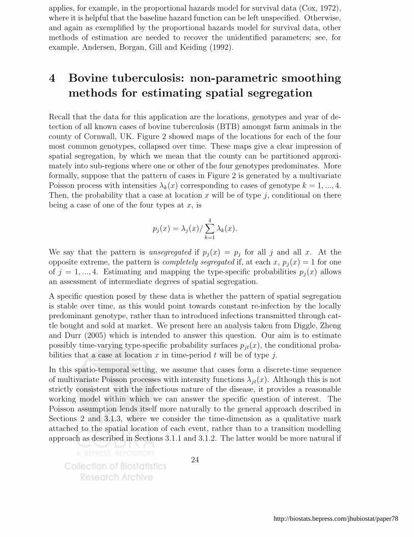
4 Bovine tuberculosis: non-parametric smoothing

methods for estimating spatial segregation

Recall that the data for this application are the locations, genotypes and year of de-tection of all known cases of bovine tuberculosis (BTB) amongst farm animals in thecounty of Cornwall, UK. Figure 2 showed maps of the locations for each of the fourmost common genotypes, collapsed over time. These maps give a clear impression ofspatial segregation, by which we mean that the county can be partitioned approxi-mately into sub-regions where one or other of the four genotypes predominates. Moreformally, suppose that the pattern of cases in Figure 2 is generated by a multivariatePoisson process with intensities λk(x) corresponding to cases of genotype k = 1, ..., 4.Then, the probability that a case at location x will be of type j, conditional on therebeing a case of one of the four types at x, is

pj(x) = λj(x)/4

∑

k=1

λk(x).

We say that the pattern is unsegregated if pj(x) = pj for all j and all x. At theopposite extreme, the pattern is completely segregated if, at each x, pj(x) = 1 for oneof j = 1, ..., 4. Estimating and mapping the type-specific probabilities pj(x) allowsan assessment of intermediate degrees of spatial segregation.

A specific question posed by these data is whether the pattern of spatial segregationis stable over time, as this would point towards constant re-infection by the locallypredominant genotype, rather than to introduced infections transmitted through cat-tle bought and sold at market. We present here an analysis taken from Diggle, Zhengand Durr (2005) which is intended to answer this question. Our aim is to estimatepossibly time-varying type-specific probability surfaces pjt(x), the conditional proba-bilities that a case at location x in time-period t will be of type j.

In this spatio-temporal setting, we assume that cases form a discrete-time sequenceof multivariate Poisson processes with intensity functions λjt(x). Although this is notstrictly consistent with the infectious nature of the disease, it provides a reasonableworking model within which we can answer the specific question of interest. ThePoisson assumption lends itself more naturally to the general approach described inSections 2 and 3.1.3, where we consider the time-dimension as a qualitative markattached to the spatial location of each event, rather than to a transition modellingapproach as described in Sections 3.1.1 and 3.1.2. The latter would be more natural if

24


the goal of the analyis was to model the transmission of the disease between farms, butthis is ruled out because of the very coarse time-resolution of the annual inspectionregime. We therefore approach the analysis of the data as a problem in non-parametricintensity estimation for a multivariate Poisson process.

The spatial distribution of farms at risk is not uniform over the county although itis, to a good approximation, constant over the twelve-year time-period covered bythe data. Also, as noted earlier, variation in the temporal intensity of the diseaseis confounded with variation in the extent of the annual testing programme. Wetherefore factorise λjt(x) as

λjt(x) = λ0(x)µ0(x, t)ρjt(x), (18)

where λ0(x) represents the spatial intensity of farms, µ0(x, t) the spatio-temporalintensity of recorded cases of unspecified type and the functions ρjt(x) representthe spatially, temporally and genotypically varying risks which are the quantities ofinterest. The type-specific probabilities associated with (18) are

pjt(x) = λjt(x)/4

∑

k=1

λkt(x) = ρjt(x)/4

∑

k=1

ρkt(x), (19)

which implies that spatio-temporal variations in the pattern of segregation can beestimated without our knowing either the spatial distribution of farms (althoughthis is available if required) or, more importantly (because it is not available), thespatio-temporal variation in the extent of the inspection programme. Note that toestimate non-specific spatial variation in risk, we would need to make the additionalassumption that µ0(x, t) = µ0(t).

We estimate the type-specific probability surfaces using a simple kernel regressionmethod. Let nt denote the number of recorded cases in time-period t. Write the datafor time-period t in the form of a set of non-specific case-locations xit : i = 1, ..., nt

and associated labels Yit giving the genotype of each case. Then, our kernel regressionestimator of pjt(x) is

pjt(x) =nt∑

i=1

wij(x)I(Yit = j), (20)

where

wij(x) = wj(x − xit)/nt∑

k=1

wj(x − xkt),

wj(x) = w(x/hj)/h2j and

w(x) = exp(−||x||2/2). (21)

The Gaussian kernel function (21) could be replaced by any other non-negative-valued weighting function. The choice of kernel function is usually less importantthan the choice of the band-width constants, hj, which determine the amount ofsmoothing applied to the data in estimating the pjt(x). Using a common set ofband-widths across time-periods makes for ease of interpretation. We shall also use

25


a common band-width, h, for all 4 components of the p-surface, as this ensures that∑m

j=1 pj(x) = 1 for every location x.

To choose the value of h, we proceed as follows. Conditioning on the case-locations,the log-likelihood for the labels Yit under the Poisson process model has the multino-mial form,

L(h) =m

∑

t=1

nt∑

i=1

m∑

j=1

I(Yit = j) log pjt(xit; h).

Maximising L(h) would give the degenerate solution h = 0. To avoid this, we use across-validated form of the log-likelihood,

Lc(h1, ..., h4) =r

∑

t=1

n∑

i=1

m∑

j=1

I(Yit = j) log p(it)jt (xit),

where p(it)jt (xi) denotes the kernel estimator (20), but based on all of the data except

(xit, Yit).

The data from the years prior to 1997 are too sparse to allow non-parametric es-timation of the pjt(x). We therefore applied the kernel regression method to datafrom the years 1997 to 2002. To maintain sufficient numbers of cases per genotypeper time-period, we also combined data from successive years to give r = 3 discretetwo-year time-periods.

The null hypothesis of interest is that pjt(x) = pj(x) for j = 1, .., 4 and t = 1, ..., r.An ad hoc statistic for a Monte Carlo test of this hypothesis is

T p =4

∑

j=1

∑

x∈X

r∑

t=1

(pj(x, t) − pj(x))2 , (22)

where X = {xti : i = 1, 2, . . . , nt; t = 1, 2, . . . , s}, pj(x, t) is the estimated type-specific

probability surface for type j in time-period t and pj(x) = r−1 ∑rt=1 pj(x, t).

The band-width which maximises the cross-validated log-likelihood is h = 9647 me-tres. A Monte Carlo test based on the statistic (22) using 999 simulations gave anattained significance level of 0.015, hence the null hypothesis is rejected at the con-ventional 5% level. However, the changes in the segregation pattern over time appearto be somewhat subtle. Figures 11, 12 and 13 show the estimated type-specific prob-ability surfaces over the three consecutive time-periods. The general pattern is of anincrease in the extent of spatial segregation over time. Thus, genotype 15 becomesprogressively more dominant in north central Cornwall, genotype 20 has establishednear-dominance in the far west by 2001/02, and spoligotype 9 is dominant in the eastof Cornwall, but within a territory which becomes more confined to an area close tothe eastern boundary as time proceeds. Finally, genotype 15 shows an apparentlystable spatial distribution over the three time-periods.

In summary, our findings from our analysis of the BTB data are that there is verystrong spatial segregation amongst the four most common genotypes, and that the

26


0.0

0.2

0.4

0.6

0.8

1.0

140000 160000 180000 200000 220000 240000

20000

40000

60000

80000

100000

120000

years 1

9

0.0

0.2

0.4

0.6

0.8

1.0

140000 160000 180000 200000 220000 240000

20000

40000

60000

80000

100000

120000

years 1

12

0.0

0.2

0.4

0.6

0.8

1.0

140000 160000 180000 200000 220000 240000

20000

40000

60000

80000

100000

120000

years 1

15

0.0

0.2

0.4

0.6

0.8

1.0

140000 160000 180000 200000 220000 240000

20000

40000

60000

80000

100000

120000

years 1

20

Figure 11: Kernel regression estimates of type-specific probability surfaces for casesin years 1997-98.

pattern of spatial segregation is broadly consistent over time, albeit with subtle butstatistically significant differences between successive two-year periods.

Further methodological developments in progress include replacing the non-parametrickernel regression methodology by a hierarchical stochastic model, in which the spatio-temporal intensities are determined by a multivariate, discrete-time log-Gaussian pro-cess, hence λj(x, t) = exp{Sj(x, t)} where {S1(x, t), ..., S4(x, t)} is a quadri-variateGaussian process. The hierarchical stochastic modelling framework is better able todeal with the relatively small numbers of cases of each genotype in each time-periodby exploiting the assumed statistical dependencies between genotypes and over time.

27


0.0

0.2

0.4

0.6

0.8

1.0

140000 160000 180000 200000 220000 240000

20000

40000

60000

80000

100000

120000

years 2

9

0.0

0.2

0.4

0.6

0.8

1.0

140000 160000 180000 200000 220000 240000

20000

40000

60000

80000

100000

120000

years 2

12

0.0

0.2

0.4

0.6

0.8

1.0

140000 160000 180000 200000 220000 240000

20000

40000

60000

80000

100000

120000

years 2

15

0.0

0.2

0.4

0.6

0.8

1.0

140000 160000 180000 200000 220000 240000

20000

40000

60000

80000

100000

120000

years 2

20


5 Real-time surveillance for gastroenteric disease:

log-Gaussian Cox process modelling

Our second application has previously been reported in greater detail by Diggle,Knorr-Held, Rowlingson, Su, Hawtin and Bryant (2003) and by Diggle, Rowlingsonand Su (2005). It concerns the development of a real-time surveillance system fornon-specific gastroenteric disease in the county of Hampshire, UK, using the datadescribed in Section 1.1.3.

The methodological problem is to build a descriptive model of the normal patternof spatio-temporal variation in the distribution of incident cases, and to use themodel to identify unusual, spatially and temporally localised, departures from thispattern, which we call “anomalies.” The wider aim is that statistical evidence ofcurrent anomalies in the spatio-temporal distribution of incident cases can then becombined with other forms of evidence, for example reports from pathology laboratoryanalyses of faecal samples, to trigger an earlier response to an emerging problem than

28


0.0

0.2

0.4

0.6

0.8

1.0

140000 160000 180000 200000 220000 240000

20000

40000

60000

80000

100000

120000

years 3

9

0.0

0.2

0.4

0.6

0.8

1.0

140000 160000 180000 200000 220000 240000

20000

40000

60000

80000

100000

120000

years 3

12

0.0

0.2

0.4

0.6

0.8

1.0

140000 160000 180000 200000 220000 240000

20000

40000

60000

80000

100000

120000

years 3

15

0.0

0.2

0.4

0.6

0.8

1.0

140000 160000 180000 200000 220000 240000

20000

40000

60000

80000

100000

120000

years 3

20


is typically achieved by current surveillance systems. For further discussion, see Diggleet al (2003).

Our descriptive model is a log-Gaussian Cox process of the kind proposed by Brix andDiggle (2001) and discussed in Section 3.2.1. Our model needs to allow for both spatialand temporal heterogeneity in the rate of calls to NHS Direct. The heterogeneityarises through a combination of factors including spatial variation in the density ofthe population at risk and aspects of the pattern of usage of NHS Direct by differentsectors of the community; for example, there is a clear day-of-the-week effect dueto the relative inaccessibility of other medical service at weekends, whilst anecdotalevidence suggests that NHS Direct is used disproportionately more often by youngfamilies than by the elderly. We assume that these spatial and temporal effects operateindependently, whereas the spatially and temporally localised anomalies which wewish to detect are governed by a spatio-temporally correlated stochastic process.Hence, within the framework of log-Gaussian Cox processes, we postulate a spatio-

29


temporal intensity function for incident cases of the form

λ(x, t) = λ0(x)µ0(t) exp{S(x, t)}, (23)

where S(x, t) is a stationary, spatio-temporal Gaussian process with expectationE[S(x, t)] = −0.5σ2, variance Var{S(x, t)} = σ2 and separable correlation functionCorr{S(x, t), S(x − u, t − v)} = ρ(u, v) = r(u) exp(−v/β). As noted earlier, thisspecification guarantees that E[exp{S(x, t)}] = 1 for all x and t. We now add theconstraint that λ0(x) integrates to 1 over the study-region. The function µ0(t) thenrepresents the time-varying total intensity, or mean number per unit time, of incidentcases over the whole county, whilst λ0(x) becomes a probability density function forthe spatial distribution of incident cases, averaged over time. The spatial correlationfunction r(u) is in principle arbitrary, but we have found that a simple exponential,r(u) = exp(−u/φ), gives a reasonable fit to the Hampshire data.

To fit the model, we need to estimate the functions λ0(x) and µ0(t), and the additionalparameters σ2, φ and β which specify the Gaussian process S(x, t). We consider eachof these estimation problems in turn.

For the spatial density λ0(x), it is hard to envisage a suitable parametric model. Also,we cannot assume that the spatial distribution of the relevant population, namelyusers of NHS Direct, matches that of the overall population distribution over thecounty of Hampshire, hence we cannot use census information to estimate λ0(x).We therefore use a non-parametric kernel density estimation method. This is verysimilar to the kernel regression method discussed in Section 4 but adapted to thedensity estimation setting. Using the Gaussian kernel (21), and band-width h, thekernel estimate of λ0(x) is

λ0(x) = n−1n

∑

i=1

h−2w{h−1(x − xi)}, (24)

where xi : i = 1, ..., n are the case-locations. Because of the very severe variations inpopulation density across the county, any choice of a fixed band-width h is liable tobe an unsatisfactory compromise between the relatively large and small band-widthswhich would be appropriate in the more rural and urban areas, respectively. Wetherefore follow a suggestion in Silverman (1985), in which we first construct a fixedband-width pilot estimator λ0(xi) using (24) with a subjectively chosen band-widthh0, then calculate g, the geometric mean of λ0(xi) : i = 1, ..., n, and use a locallyadaptive kernel estimator

λ0(x) = n−1∑

h−2i φ{(x − xi)/hi}

with hi = h0{λ0(xi)/g}−0.5. This has the required effect of applying a larger band-

width in the more rural areas, where λ0(x) is relatively small. Figure 14 shows theresulting estimate λ0(x).

To estimate the mean number of cases per day, µ0(t), a parametric approach is morereasonable. We use a Poisson log-linear regression model incorporating day-of-the-week effects as a 7-level factor, time-of-year effects as sine-cosine wave at frequency

30


420 440 460 480

100

120

140

160

Northing (Kilometers)

Eas

ting

(Kilo

met

ers)

00.000720.00140.00220.00290.00360.00430.00510.00580.0065

Figure 14: Locally adaptive kernel estimate of λ0(x) for the Hampshire gastroentericdisease data.

ω = 2π/365, plus its first harmonic, and a linear trend to reflect progressive up-takein the usage of NHS Direct during the period covered by the data. Hence,

log µ0(t) = δd(t) + α1 cos(ωt) + η1 sin(ωt) + α2 cos(2ω) + η2 sin(2ωt) + γt, (25)

where d(t) codes the day of the week. The Poisson formulation does not account forthe extra-Poisson variation which, as anticipated, the data exhibit, but neverthelessproduces consistent estimates on the assumption that (25) is a correct specificationfor µ0(t). Figure 15 compares the resulting estimate, centred on the average of theseven daily intercepts δd(t), with the observed numbers of calls per day, averaged overeach week. The spring peak in incidence is a well-known feature of this group ofdiseases.

To estimate the parameters of the stochastic component of the model, S(x, t), wehave used a simple method-of-moments approach, based on matching empirical andtheoretical second-moment properties of the data and model, respectively. We are cur-rently developing an implementation of a Monte Carlo maximum likelihood method,based on material in Moller and Waagepetersen (2004). A partial justification for themethod-of-moments approach is that the main goal of the analysis is real-time spatialprediction, whose precision is limited by the relatively low daily incidence of cases,whereas parameter estimation draws on the complete set of data; hence, efficiency ofparameter estimation is not crucial.

31


46

810

1214

1618

Jan 01 Apr 01 Jul 01 Oct 01 Jan 02 Apr 02 Jul 02 Oct 02 Dec 02

PSfrag

replacem

ents

µ0(t

)

Figure 15: Fitted log-linear model for the mean number of gastroenteric disease casesper day adjusted for day-of-the-week effects (solid line), and observed numbers ofcases per day averaged over successive weeks (solid dots).

Consider first the parameters of the spatial covariance structure of S(x, t), namely

Cov{S(x, t), S(x − u, t)} = σ2 exp(−|u|/φ).

The corresponding spatial pair correlation function is g(u) = exp{σ2 exp(−|u|/φ)},and the estimation method consists of minimising the criterion

∫ u0

0[{log g(u)} − {log g(u)}]2du, (26)

where u0 = 2km is chosen subjectively as the apparent range of the spatial correlation,and g(u) is a non-parametric estimate of the pair correlation function. We use a time-averaged kernel estimator,

g(u) =1

2πuT |A|

T∑

t=1

n∑

i=1

∑

i6=j

Kh(u− ‖ xi − xj ‖)wij

λt(xi)λt(xj). (27)

In (27), each of the summations over i 6= j refers to pairs of events occurring on thesame day, T is the length of the study-period, A the study area, wij is Ripley’s (1977)

edge-correction as used in (4), λt(x) = λ0(x)µ0(t) and

Kh(u) =

{

0.75h−1(1 − u2/h2) : −h ≤ u ≤ h: otherwise.

32


To estimate the temporal correlation parameter β, we again match empirical andtheoretical second-moment properties, as follows. Let Nt denote the numbers of inci-dent cases on day t. For our model, the time-variation in µ0(t) makes the covariancestructure of Nt non-stationary. We obtain

Cov(Nt, Nt−v) = µ0(t)1(v = 0) + {µ0(t)µ0(t − v)} ×

{∫

W

∫

Wλ0(x1)λ0(x2) exp[σ2 exp(−v/β) exp(−u/φ)]dx1dx2 − 1}

(28)

Note that the expression for Cov(Nt, Nt−v) given by Brix and Diggle (2001) is incor-rect. To estimate β we minimise

v0∑

v=1

n∑

t=v+1

{C(t, v) − C(t, v; β)}2,

where v0 = 14 days, C(t, v) = NtNt−v − µ0(t)µ0(t− v) and C(t, v; θ) = Cov(Nt, Nt−v)as defined in (28) but plugging in the previously estimated values for σ2 and φ.

The resulting estimates are shown in Figure 16. Note in particular that the scaleson which the spatial and temporal dependence decay are broadly consistent withthe known character of the diseases in question, which are spread by direct contactbetween infected individuals and generally have latent periods of the order of a fewdays.

We now use the fitted model for spatial prediction, as follows. Firstly, and withthe same justification as given above for the use of potentially inefficient methodsof parameter estimation, we use plug-in values of the estimated model parameters,thereby ignoring the effects of parameter uncertainty on the predictive distributions ofinterest. We then use a Metropolis-adjusted Langevin algorithm, as described in Brixand Diggle (2001), to generate samples from the conditional distribution of S(x, t)given data up to time t. For display purposes, we choose a critical threshold valuec > 1 and map predictive exceedance probabilities,

pt(x) = P (exp{S(x, t)} > c|data) (29)

We would argue that mapping pt(x) is more relevant than mapping predictive es-timates, S(x, t). The latter are highly variable because of the relatively low dailyincidence and would be liable to over-interpretation. We suggest that the value of cshould be chosen by the public health practitioner to represent a multiplicative in-crease in the local daily incidence which, if verified, would be regarded as practicallysignificant. A high predictive probability that this threshold has been exceeded at aparticular time and place would then suggest that some kind of follow-up action maybe required, for example to ascertain whether recent cases in the immediate vicinitymight have a common cause, or are more likely to be unrelated chance occurrences.

Figure 17 shows an example of the resulting map of pt(x) for one day in March 2003,using the threshold value c = 2. Note that the colour-scale for pt(x) is continuous,

33


0.0 0.5 1.0 1.5 2.0

−1

01

23

45

Distance(Kilometers)

Log

Pai

r C

orre

latio

n F

unct

ion

FittedEmpirical

0 2 4 6 8 10 12 14

−1

01

23

4

Time lag(Days)

Aut

ocov

aria

nce

func

tion

FittedEmpirical

Figure 16: Empirical (solid line) and fitted (dashed line) second-moment properties forthe Hampshire gastroenteric disease data. The left-hand panel shows the logarithmof the pair correlation function, the right-hand panel the temporal autocovariancefunction.

but non-linear so that only predictive probabilities close to 1 show up as orange orred. We also emphasise that the value c = 2 was chosen for illustrative purposesand is much smaller than would be associated, in this application, with a genuineoutbreak of public health concern.

As noted above, one way to refine the methodology associated with this applicationwould be to use Monte Carlo maximum likelihood estimation for the covariance pa-rameters of S(x, t). A brief outline of this method follows. We approximate thecontinuous spatio-temporal domain A× (0, T ) by a fine lattice, and denote by X andS the point process data and the latent Gaussian process in this discretised domain.The likelihood for the model, L(θ; X) say, is the marginal distribution of X, which isintractable, whereas the joint distribution of X and S can be written explicitly as theproduct of the conditional distribution of X given S and the marginal distribution ofS, both of which have known standard forms – Poisson and Gaussian, respectively.It follows that for any fixed value θ0,

L(θ; X) =∫

f(S, X; θ)dS

=∫

f(S, X; θ) ×L(θ0; X)

L(θ0; X)×

f(S, X; θ0)

f(S, X; θ0)dS

34


Figure 17: Predictive exceedance probabilities pt(x) for the Hampshire gastroentericdisease data on a day in March 2003, using the threshold value c = 2. Incident casesover five consecutive days are shown as circles of diminishing size to correspond tothe progressive discounting of past data in constructing the predictive distribution ofS(x, t).

= L(θ0; X)∫

f(S, X; θ)

f(S, X; θ0)f(S|X; θ0)dS.

Hence, the likelihood ratio between θ and θ0 is

L(θ; X)/L(θ0; X) = Eθ0

[

f(S, X; θ)

f(S, X; θ0)

]

, (30)

where Eθ0[·] denotes expectation with respect to the conditional distribution of S

given X at θ = θ0. In (30), we now replace the theoretical expectation by a samplemean over Monte Carlo simulations, using the same Metropolis-adjusted Langevinalgorithm as used earlier to simulate samples from the predictive distribution of Sgiven X. Note also that writing S = a(θ) + B(θ)Z, where Z is a vector of in-dependent standard Gaussian variates, gives f(S, X; θ) = f(X|Z; θ)f(Z), in whichcase the ratio within the expectation term on the right hand side of (30) reduces tof(X|Z; θ)/f(X|Z; θ0).

Another possible refinement of the methodology would be to use a stochastic modelof daily incidence in place of the deterministic µ0(t). In particular, the rising trend

35


evident during the two-year period covered by the data which were used to developthe model was not sustained thereafter. More generally, patterns in the usage of NHSDirect are liable to fluctuate in response to changes in policy-related factors withinthe NHS system whose combined effects are hard to capture in a deterministic model.A pragmatic strategy would be the following. Postulate a temporal log-Gaussian Coxprocess for the daily incident counts, Nt, as a series of conditionally independentPoisson counts with conditional expectations exp(αt + Mt), where αt encodes day-of-the-week effects and Mt is a latent Gaussian process. Use this model to generatereal-time predictions αt + Mt, which can then be plugged into the spatial predictionalgorithm in place of the log-linear regression estimates µ0(t).

6 Foot-and-mouth disease: mechanistic modelling

and partial likelihood analysis

To illustrate the partial likelihood method described in Section 3.2.2, we analyse thefoot-and-mouth data using a mechanistic model proposed by Keeling et al (2001).The analysis reported here is taken from Diggle (2005).

The model assumes that the rate of transmission of infection between an infectedfarm i and a susceptible farm j is given by

λij(t) = λ0(t)AiBjf(||xi − xj||)Iij(t), (31)

where λ0(t) is a baseline rate of infection, Ai and Bj encode characteristics of thefarms in question which affect their infectivity and susceptibility respectively, f(·) isa transmission kernel which models the spread of infection as a function of distance,and Iij(t) is an indicator that farm i is infective and farm j susceptible at time t.The data include, as applicable for each animal-holding farm, the dates on whichthe disease was reported and on which the stock was culled. To allow for reportingdelays, we assume that a farm is reported as a case τ days after it becomes infective.A farm remains infective unless and until its stock is culled. A farm is susceptible ifit is not infective, and has not had its stock culled.

In the analysis reported here, we assume that τ = 5 days and model the infectivityand susceptibility factors as

Ai = (αn1i + n2i) (32)

andBj = (βn1i + n2i). (33)

where n1i and n2i are the numbers of cows and sheep held by farm i at the start of theepidemic. The parameters α and β therefore represent the relative infectiousness andsusceptibility, respectively, of cows to sheep. For the transmission kernel, we assumethat

f(u) = exp{−(u/φ)κ} + ρ. (34)

36


Keeling et al (2001), did not specify a functional form for f(·), but (34) captures thequalitative features of the results which they reported in graphical form. In particular,they reported a sharper-than-exponential decay with distance, which in (34) wouldcorrespond to κ < 1, whilst ρ in (34) represents the contribution to the epidemic fromapparently spontaneous cases which occur remotely from any previous case.

For any farm k, we define λk(t) =∑

j λjk(t), from which we obtain the conditionalintensities

λ(xi, ti|Hti) = λi(ti)/∑

k

λk(ti).

The partial log-likelihood follows by substitution of the conditional intensities into(16) and (17). To maximise the partial log-likelihood we use the Nelder-Mead simplexalgorithm (Nelder and Mead, 1965) as implemented in the R function optim(), whichprovides a numerical estimate of the Hessian matrix.

In the model for the transmission kernel, the parameters κ and ρ are poorly identifiedbecause the cases which appear to correspond to long-range transmission are few innumber, and can be explained empirically either by including a small, positive valueof ρ or by adjusting the value of κ. Because ρ corresponds formally to what is knownto be a real effect, namely the indirect spread of infection via the movement of farmequipment and staff, we retain ρ as a positive-valued parameter to be estimated,but fix κ = 0.5 to correspond to the observation in Keeling et al (2001) that thetransmission kernel is more sharply peaked than exponential.

We first investigated whether the data in Cumbria and Devon support the assumptionof a common set of parameters in the two counties. The likelihood ratio test statisticfor common versus separate parameters is 2.98 on 4 degrees of freedom, hence p = 0.56and we therefore accepted the hypothesis of common parameter values. We thenobtained common parameter estimates (α, β, φ, ρ) = (4.92, 30.68, 0.39, 9.9 × 10−5).For all practical purposes, ρ ≈ 0, although a likelihood ratio test formally rejectsρ = 0 because the likelihood is sensitive to the precise probabilities which the modelassigns to rare events.

One question of specific interest is whether the infectivities and susceptibilities forindividual farms, Ai and Bj, are linear or sub-linear in the numbers of animals. Toinvestigate this, we extend (32) and (33) to Ai = (αnγ

1i + nγ2i) and Bj = (βnγ

1i + nγ2i),

respectively, where γ is an additional parameter to be estimated. Fitting this five-parameter model results in a large increase in the maximised log-likelihood, from−6196.3 to −5861.4.

Another possible extension of the model would be to include farm-level covariatesby defining Ai = (αnγ

1i + nγ2i) exp(z′iδ), where zi is a vector of covariates for farm

i, with a similar expression for the susceptibilities Bj. The zi might, for example,codify management practices or other measured characteristics of individual farmswhich could affect their propensity to transmit, or succumb to, the disease. Byway of illustration, we consider adding a log-linear effect of farm area to the model.The likelihood ratio statistic for the covariate effect is 3.26 on 1 degree of freedom,

37


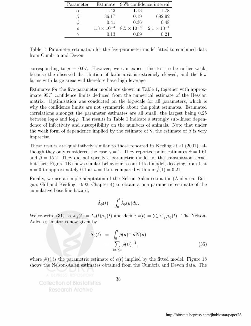
Parameter Estimate 95% confidence intervalα 1.42 1.13 1.78β 36.17 0.19 692.92φ 0.41 0.36 0.48ρ 1.3 × 10−4 8.5 × 10−5 2.1 × 10−4

γ 0.13 0.09 0.21

Table 1: Parameter estimation for the five-parameter model fitted to combined datafrom Cumbria and Devon

corresponding to p = 0.07. However, we can expect this test to be rather weak,because the observed distribution of farm area is extremely skewed, and the fewfarms with large areas will therefore have high leverage.

Estimates for the five-parameter model are shown in Table 1, together with approx-imate 95% confidence limits deduced from the numerical estimate of the Hessianmatrix. Optimisation was conducted on the log-scale for all parameters, which iswhy the confidence limits are not symmetric about the point estimates. Estimatedcorrelations amongst the parameter estimates are all small, the largest being 0.25between log φ and log ρ. The results in Table 1 indicate a strongly sub-linear depen-dence of infectivity and susceptibility on the numbers of animals. Note that underthe weak form of dependence implied by the estimate of γ, the estimate of β is veryimprecise.

These results are qualitatively similar to those reported in Keeling et al (2001), al-though they only considered the case γ = 1. They reported point estimates α = 1.61and β = 15.2. They did not specify a parametric model for the transmission kernelbut their Figure 1B shows similar behaviour to our fitted model, decaying from 1 atu = 0 to approximately 0.1 at u = 1km, compared with our f(1) = 0.21.

Finally, we use a simple adaptation of the Nelson-Aalen estimator (Andersen, Bor-gan, Gill and Keiding, 1992, Chapter 4) to obtain a non-parametric estimate of thecumulative base-line hazard,

Λ0(t) =∫ t

0λ0(u)du.

We re-write (31) as λij(t) = λ0(t)ρij(t) and define ρ(t) =∑

i

∑

j ρij(t). The Nelson-Aalen estimator is now given by

Λ0(t) =∫ t

0ρ(u)−1dN(u)

=∑

i:ti≤t

ρ(ti)−1, (35)

where ρ(t) is the parametric estimate of ρ(t) implied by the fitted model. Figure 18shows the Nelson-Aalen estimates obtained from the Cumbria and Devon data. The

38


50 100 150 200

0.00

00.

005

0.01

00.

015

0.02

0

time (days since 1 Feb)

cum

ulat

ive

haza

rd

Figure 18: Estimated cumulative baseline hazards in Cumbria (solid line) and inDevon (dotted line) for the five-parameter model.

generally lower estimates for Devon are consistent with the lower overall prevalenceof the disease (137 cases out of 8182 at-risk farms in Devon, 657 cases out of 5090at-risk farms in Cumbria). Both estimates are approximately linear over the first twoto three months, by which time the epidemic in Devon has almost run its course.The slope of the Cumbria estimate increases thereafter. This does not necessarilyimply a failure of the culling strategies being applied, since the model already takesaccount of their effects, but rather suggests that external environmental effects, forexample the increase in animal movements outdoors in spring and summer, may havepromoted an increase in the virulence of the disease process.

This analysis of the foot-and-mouth data demonstrates the feasibility of using thepartial likelihood approach to answer a variety of questions relevant to an under-standing of the underlying disease process. The method of fitting is quite flexible,and it would be straightforward to extend the model in various ways, for exampleby including additional farm-level covariates. A fuller analysis of the data will bereported separately. More generally, the partial likelihood provides a useful methodfor analysing any spatio-temporal point process model which which is specified viaits conditional intensity function. The method is based on a generally accepted prin-ciple of inference with known asymptotic properties, whilst being computationallystraightforward and therefore well-suited to routine use.

39


7 Discussion

In this chapter, we have tried to indicate the scope for simple adaptation of existingmethods, and for development of new methods, to analyse spatio-temporal pointprocess data. Data-sets of this kind are becoming more widely available, perhapsreflecting the increased ability in many fields of science to capture such data routinely.More fundamentally, interesting scientific questions concerning the dynamic spatio-temporal behaviour of natural systems cannot easily be addressed using purely spatialor temporal information.

In the author’s opinion, simple adaptations of existing spatial statistical methods,as illustrated by our analysis of the bovine tuberculosis data, will continue to bevaluable for descriptive analysis, and are more or less forced on us when the dataare coarsely discretised in time. But when data with a fine resolution in both thespatial and temporal dimensions are available, models which explicitly recognise thedirectional nature of time by conditioning future behaviour on past outcomes arelikely to be more insightful. Our analyses of the gastroenteric disease data and ofthe foot-and-mouth data illustrate this general philosophy. For the gastroentericdisease application our model for the latent stochastic process S(x, t) is, essentially,a multivariate time series model incorporating a qualitatively sensible, if admittedlyalso computationally convenient, Markov dependence structure in time. The cross-correlation structure of the model is then chosen so as to have a parsimonious spatialinterpretation whilst giving a reasonable empirical fit to the data. In contrast, forthe foot-and-mouth data we use a previously proposed mechanistic model in whichthe conditioning on past events is used explicitly to quantify the current risk oftransmission of the disease from an infective to a susceptible farm.

As in other areas of statistics, the development of computationally intensive, MonteCarlo methods of inference has greatly enhanced our ability to fit relatively complexand realistic models. However, it is still all too easy to find combinations of dataand model for which fitting by Monte Carlo methods is computationally infeasible.Also, the requirement to tune Monte Carlo algorithms to each non-standard applica-tion imposes very real constraints on the statistician’s ability to compare a range ofcandidate models within a reasonable time-scale whilst ensuring that Markov chainMonte Carlo algorithms have converged to their equilibrium distributions and thatinferences about parameter combinations of interest are appropriately insensitive topragmatic choices of multivariate priors. For these reasons, we see a place for methodsof inference such as the partial likelihood method proposed in Diggle (2005) and ap-plied here to the foot-and-mouth data, which are capable of routine implementationwhilst still being based on generally accepted statistical principles.

40


Acknowledgements

This work was supported by the UK Engineering and Physical Sciences ResearchCouncil through the award of a Senior Fellowship to Peter Diggle (Grant numberGR/S48059/01) and by the USA National Institute of Environmental Health Sci-ence through Grant number 1 R01 ES012054, Statistical Methods for EnvironmentalEpidemiology.

I thank Prof. Abbie Hughes and Dr. Elzbieta Wieniawa Narkiewicz for providingthe amacrine cell data, and Laura Green, Matt Keeling, Graham Medley, Sir DavidCox and Hugues Lassalle for very helpful discussions concerning the foot-and-mouthdata.

The application to the bovine tuberculosis data was supported by the UK Departmentfor Environment, Food and Rural Affairs (Grant number SE3020). Roger Sainsbury ofthe State Veterinary Service helped collect the data. Jackie Inwald of the Departmentof Bacterial Diseases, VLA Weybridge, carried out the spoligotyping.

The application to gastroenteric disease surveillance was supported by a grant fromthe Food Standards Agency, UK, and from the National Health Service ExecutiveResearch and Knowledge Management Directorate.

References

Andersen, P.K., Borgan, O., Gill, R.D. and Keiding, N. (1992). Statistical ModelsBased on Counting Processes. New York : Springer.

Banerjee, S., Carlin, B.P and Gelfand, A.E. (2003). Hierarchical Modelling and Anal-ysis for Spatial Data. London: CRC Press.

Besag, J. (1974). Spatial interaction and the statistical analysis of lattice systems(with Discussion). Journal of the Royal Statistical Society B 36, 192–225.

Bhopal, R.S., Diggle, P.J. and Rowlingson, B.S. (1992). Pinpointing clusters of ap-parently sporadic cases of legionnaires’ disease. British Medical Journal, 304, 1022-7.

Brix, A. and Diggle, P.J. (2001). Spatio-temporal prediction for log-Gaussian Coxprocesses. Journal of the Royal Statistical Society, B 63, 823–41.

Brix, A. and Diggle, P.J. (2003). Corrigendum: Spatio-temporal prediction for log-Gaussian Cox processes. Journal of the Royal Statistical Society, B 65, 946.

Brown, P.E., Karesen, K., Roberts, G.O. and Tonellato, S. (2000). Blur-generatednon-separable space-time models. Journal of the Royal Statistical Society, B 62,847–60.

Cooper, D.L., Smith, G.E., O’Brien, S.J., Hollyoak, V.A. and Baker, M. (2003). Whatcan analysis of calls to NHS Direct tell us about the epidemiology of gastrointestinal

41


infections in the community? Journal of Infection, 46, 101–5.

Cox, D.R. (1972). Regression models and life tables (with Discussion). Journal ofthe Royal Statistical Society B, 34, 187–220.

Cox, D.R. (1975). Partial likelihood. Biometrika, 62, 269–75.

Cox, D.R. (1977). The role of significance tests. Scandinavian Journal of Statistics,4, 49–71.

Cressie, N.A.C. (1991). Statistics for Spatial Data. New York : Wiley.

Daley D J and Vere-Jones D (1988). An Introduction to the Theory pf Point Processes.New York : Springer.

Diggle, P.J. (2003). Statistical Analysis of Spatial Point Patterns (second edition).London : Arnold.

Diggle, P.J. (2005). A partial likelihood for spatio-temporal point processes. JohnsHopkins University, Department of Biostatistics Working Papers, Working Paper 75.http://www.bepress.com/jhubiostat/paper75

Diggle, P.J., Chetwynd, A.G., Haggkvist, R. and Morris, S. (1995). Second-orderanalysis of space-time clustering. Statistical Methods in Medical Research, 4, 124-36.

Diggle, P.J., Eglen, S.J. and Troy, J.B. (2005). Modelling the bivariate spatial distri-bution of amacrine cells. In Case Studies in Spatial point Processes, ed A. Baddeley,J. Mateu, D. Stoyan. New York : Springer (to appear).

Diggle, P.J., Knorr-Held, L., Rowlingson, B., Su, T., Hawtin, P. and Bryant, T.(2003). Towards On-line Spatial Surveillance. In Monitoring the Health of Popula-tions: Statistical Methods for Public Health Surveillance., ed R. Brookmeyer and D.Stroup. Oxford : Oxford University Press.

Diggle, P.J., Rowlingson, B. and Su, T-L. (2005). Point process methodology foron-line spatio-temporal disease surveillance. Environmetrics, 16, 423–34.

Diggle, P.J., Zheng, P. and Durr, P. (2005). Non-parametric estimation of spatialsegregation in a multivariate point process. Applied Statistics, 54, 645–58.

Durr, P.A., Hewinson, R.G. and Clifton-Hadley, R.S. (2000). Molecular epidemiologyof bovine tuberculosis: I. Mycobacterium bovis genotyping. Revue Scientifique etTechnique de l’office Internationale des Epizooties, 19, 675–688.

Geyer, C.(1999). Likelihood inference for spatial point processes. In Stochastic Ge-ometry: likelihood and computation, ed O.E. Barndorff-Nielsen, W.S. Kendall andM.N.M. van Lieshout, 79–140.

Geyer, C.J. and Thompson, E.A. (1992). Constrained Monte Carlo maximum likeli-hood for dependent data (with Discussion). Journal of the Royal Statistical Society,B 54, 657–99.

Gneiting, T. (2002). Nonseparable, stationary covariance functions for space-time

42


data. Journal of the American Statistical Association, 97, 590–600.

Hughes, A. (1985) New perspectives in retinal organisation. Progress in Retinal Re-search 4 243–314.

Keeling, M.J., Woolhouse, M.E.J., Shaw, D.J., Matthews, L., Chase-Topping, M.,Haydon, D.T., Cornell, S.J., Kappey, J., Wilesmith, J. and Grenfell, B.T. (2001).Dynamics of the 2001 UK foot and mouth epidemic: stochastic dispersal in a hetero-geneous landscape. Science, 294, 813–7.

Moller, J. and Sorensen, M. (1994). Statistical analysis of a spatial birth-and-deathprocess model with a view to modelling linear dune fields. Scandinavian Journal ofStatistics, 21, 1–19.

Moller, J. and Waagepetersen, R.P. (2004). Statistical Inference and Simulation forSpatial Point Processes. London : Chapman and Hall.

Moller, J., Syversveen, A. and Waagepetersen, R. (1998). Log Gaussian Cox pro-cesses. Scandinavian Journal of Statistics, 25, 451–82.

Nelder, J.A. and Mead, R. (1965). A simplex algorithm for function minimisation.Computer Journal, 7, 308–13.

Neyman, J. and Scott, E.L. (1958). Statistical approach to problems of cosmology.Journal of the Royal Statistical Society, Series B 20, 1–43.

Peebles, P.J.E. and Groth, E.J. (1975). Statistical analysis of catalogs of extragalacticobjects, V. Three point correlation function for the galaxy distribution in the Zwickycatalog. Astrophysical Journal, 196, 1–11.

Ripley, B.D. (1976). The second-order analysis of stationary point processes. Journalof Applied Probability, 13, 255–66.

Ripley, B.D. (1977). Modelling spatial patterns (with discussion). Journal of theRoyal Statistical Society B 39, 172–212.

Rue, H. and Held, L. (2005). Gaussian Markov Random Fields: Theory and Appli-cations. London: CRC Press.

UK National Audit Office (2002). The 2001 Outbreak of Foot and Mouth Disease.Report by the Comptroller and Auditor General, HC 939, Session 2001–2002. London:The Stationery Office.

43


spatio-temporal point processes: methods and applicationsevents which occur within a pre-speci ed...

Documents