SPECIFICATION AND CONSTRUCTION OF MACHINES

J.R. Abrial

Rapporteur: Mr. B.C. Haapshere

Abstract:

Specification and construction of sequential programs, although not entirely mastered, have now entered a more mature phase characterised by the recognition of a small set of well defined program constructs (sequencing, alternation, loop, and so on) together with the corresponding proof rules, and also by the definition of well defined and powerful specification and construction methods (pre-post-conditions, abstract­ion/implementation, combination of specifications, abstract data types, algebraic specifications, and so on).

The situation is certainly quite different for parallel processes. Although significant results have been obtained in recent years, there does not seem to exist a wide agreement about what the essential features of parallelism should be. (As an indication of this fact it is interesting to compare the var ious ways parallelism was handled in the four DOD coloured languages) Consequently one could hardly speak of well defined specification and construction methods, although some very spectacular results have been obtained here and there.

This talk is concerned with such questions as - Does it make sense to think of specifying processes which are supposed to run for ever? If yes, to specify what? Does there exist a way of "connecting" specifications in the same way as we connect processes, etc.?

The speaker will try to answer these kinds of questions and to study and illustrate a few examples.

5

SPECIFICATION AND CONSTRUCTION

OF MACHINES

1. - WHAT IS A PROGRAM ?

In order to narrow the spectrum of possible answers to such a broad question, it might be advisable to choose a specific point of view. For instance, an interesting point of view might be that of the mathematician. In other words, by the question

What is a Program, from a Mathematical Point of View ?

we are not concerned by such activities as, say, the translation of programs from one Programming Language to the other or by the interpretation of programs by Machines ; rather, we are interested in those definitions of the program concept which are relevant to the main activity of the mathematician, that is, that of performing proofs.

The link between our intuitive understanding of programs and a possible answer to the previous question is given by the well­known mathematical concept of homogeneous binary relation. More precisely, a program might be said to establish a relationship between the values of its variables before and after its execution. For instance, let, by convention, the mathematical variable x (Xl)

denote the value of the programming variable x before (after) the execution of the program

x := x + 1

If this is the case, then these two values are obviously related to each other by the following condition

Xl = X + 1

It is traditional, 1n Mathematics, to write the form

x R Xl

for expressing that x and Xl are related by a certain relation R consequently we shall write

6

x (x := x + I) Xl

for expressing that x and Xl are "related" by the program

x := x + I

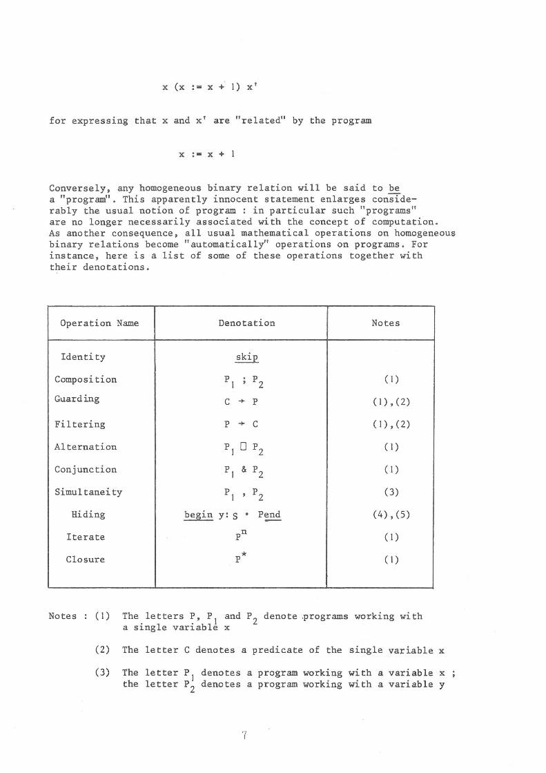
Conversely, any homogeneous binary relation will be said to be a "program". This apparently innocent statement enlarges conside­rably the usual notion of program : in particular such "programs" are no longer necessarily associated with the concept of computation. As another consequence, all usual mathematical operations on homogeneous binary relations become "automatically" operations on programs. For instance, here is a list of some of these operations together with their denotations.

Operation Name Denotation Notes

Identity skip

Composition PI ; P2 ( I)

Guarding C -+ P (1),(2)

Filtering P -+ C (1),(2)

Alternation PI 0 P2 ( I)

Conjunction PI & P2 ( I )

Simultaneity PI ' P2 (3)

Hiding begin y: S . Pend (4) , (5) -Iterate pn ( I )

Closure P * ( I )

Notes (I) The letters P, PI and P2 denote .programs working with a single variable x

(2) The letter C denotes a predicate of the single variable x

(3) The letter PI denotes a program working with a variable x the letter P2 denotes a program working with a variable y

7

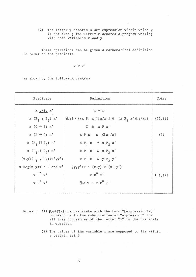
(4) The letter S denotes a set expression within which y is not free ; the "letter P denotes a .program working with both variables x and y

These operations can be given a mathematical definition ~n terms of the predicate

x P x'

as shown by the following diagram

Predicate Definition Notes

x skip x' x = x' "\

X (P I • P ) x' , 2 3z: S • «x PI x')[Z/X ' ] & (x P2 x')[z/x]) (1),(2)

x (C + P) x' C & x P x'

x (p + C) x' x P x' & C[x' /x] ( I )

x (P lOP 2) x' x PI x' v x P2 x'

x (PI .& P2) x' x PI x' & x P2 x'

(x,y)(P I , P2)(X ' ,y') x PI x' & Y P2 y'

X begin y:T • P end x' -- 3y,y' :T • (x,y) P (X',y')

x pn x' x Rn x' (3),(4)

* x P

Notes

x' 3n:N • x pn x'

(I) Postfixing a predicate with the form "[ expression/x]" corresponds to the substitution of "expression" for a11 free occurences of the letter "x" in the predicate in question

(2) The values of the variable x are supposed to lie within a certain set S

8

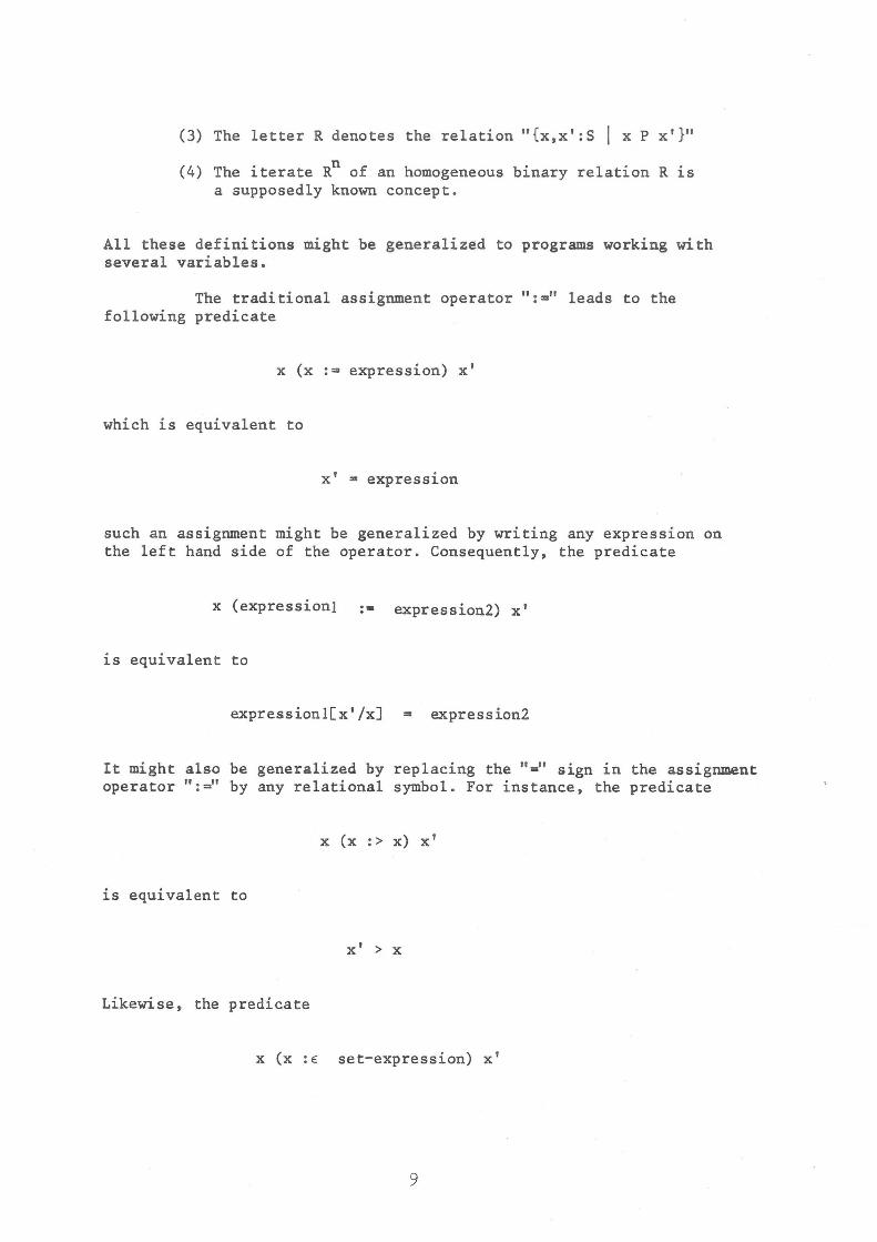
(3) The letter R denotes the relation n{x,x':S I x p x'}n

(4) The iterate Rn of an homogeneous binary relation R is a supposedly known concept.

All these definitions might be generalized to programs working with several variables.

The traditional assignment operator n: .. n leads to the following predicate

x (x := expression) x'

which ~s equivalent to

x' .. expression

such an assignment might be generalized by wr~t~ng any expression on the left hand side of the operator. Consequently, the predicate

x (expression! :a expression2) x'

~s equivalent to

expressionl[x'/x] ~ expression2

It might also be generalized by replacing the n=n sign in the assignment operator n:=n by any relational symbol. For instance, the predicate

x (x :> x) x'

is equivalent to

x' > x

Likewise, the predicate

x (X:E set-expression) x'

9

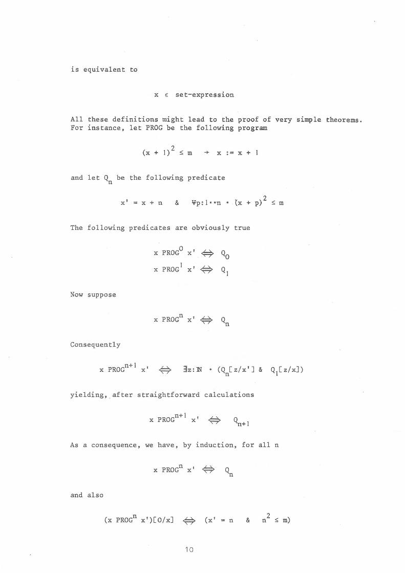
is equivalent to

X E: set-expression

All these definitions might lead to the proof of very simple theorems. For instance, let PROG be the following program

(x + 1)2 ::;; m -+ x := x + 1

and let Q be the following predicate n

x' = x + n & 2 Vp:loon ° tx + p) ::;; m

The following predicates are obviously true

Now suppose

Consequently

x PROGO

x' <# QO

x PROG1

x' # Q1

n x PROG x' # Qn

x PROGn+

1 x' ~

yielding, after straightforward calculations

x PROGn+1 x' ~ Q ~ n+1

As a consequence, we have, by induction, for all n

and also

(x PROGn x')[O/x] # (x' = n & 2

n ::;; m)

10

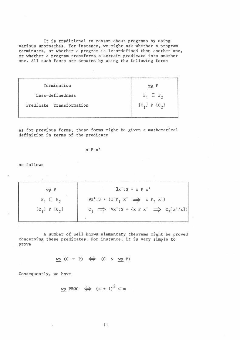
It is traditional to reason about programs by using various approaches. For instance, we might ask whether a program terminates, or whether a program is less-defined than another one, or whether a program transforms a certain predicate into another one. All such facts are denoted by using the following forms

Termination

Less-definedness

Predicate Transformation

~P

PI [ P2

{ell P {e2}

As for previous forms, these forms might be given a mathematical definition in terms of the predicate

x P Xl

as follows

~P 3x l: S • x P Xl

PI [ P2 VXl: S • (x PI Xl =} x P2

Xl)

{ell P {e2} Cl =} ¥Xl:S • (x P Xl =} C2[ x I Ix])

A number of well known elementary theorems might be proved concerning these predicates. For instance, it is very simple to prove

~ (C -+ P) -# (C & wp P)

Consequently, we have

~ PROG -# (x + I) 2 ~ m

11

Certain classical program constructs might be defined in terms of the above definitions. For instance, the loop of a program P, denoted after E.W. Dijkstra

do P od

~s defined as

p* -+ -, ~ P

Consequently, the predicate

x (do P od) x'

~s equivalent to

3x: N • x pn x' & (-,wp p)[x'/x]

For instance, the predicate

x (do PROG od) x'

is equivalent to

3n: N • Q n

yielding, for x = 0

& 2 m < (x' + 1)

3n:N • x' = n & n2 ::; m < (x' + 1)2

that ~s

We have then just proved that the program

12

do (x + 1)2 ~ m ~ x:= x + 1 od

results, when "started" with x = 0, in the integer square root of the parameter m.

2. - WHAT IS A MACHINE?

Over the past few years, it has become fashionable to distribute computer processing among several inter-connected machines. An interesting challenge, raised by the building of such structures, is the discovery of a "good" mathematical model that could help prove their properties in a systematic way.

In order to do so, one of the first questions that comes to mind ~s obviously the following

What ~s a Machine ?

To such a very general question, an equally general answer can only be given; in fact, observing the run of a machine through its "visible" registers, and recording what happens and also when it happens, results in the production, after the machine has stoppe~f a complete record of its "visible" behavior: in other words, the machine has been a mere producer of its past.

More precisely, we shall consider the history of events which occur on each visible register (henceforth called channel) of a running machine. Such histories will be represented by finite functions, the domains of which are subsets of the positive Natural Numbers. In fact, these numbers simply denote some measurements of the time (in some arbitrary unit) relative to the starting date of the machine.

For instance, we might observe that the following history records the past of a machine with a single channel "in".

~n = {1 ~ a , 3 ~ b , 4 ~ c , 7 ~ d}

Hence, at time 1, "event a" has occured, then, later, at time 3, "event b" has occured, and so on.

Another machine, called A, has "produced" the following pasts on its channels "in" and "out"

~n = {1 ~ a 3 ~ b 4 ~ c 7 ~ d}

out = {2 ~ a 5 ~ c 8 ' ,+ d " 9 ~ d}

On these records, we can see that each event occuring on channel " out", at, say, time t, has already occured on channel "in" ; more precisely, this event was the last aneta occur, before t, on channel "in" •

The following two histories are produced by a machine called B

1.n = {I -+- a 3 -+- b 4 -+- C 7 -+- d}

out = {2 -+- a 4 -+- b 8 -+- C 9 -+- d}

On these records, we can observe that all events occuring on channel "in", later occur on channel "out" in the same time order. Also, machine B, unlike machine A, may "produce" two events at the same time on distinct channels.

Our next example shows the following record for a machine called C

in = {I -+- a 3 -+- b 4 -+- C 7 -+- d}

out = {2 -+- a 6 -+- C 7 -+- b 9 -+- d}

This machine looks like our previous machine B in that all events occuring on channel "in" later occur on channel "out" ; however, the time order is not preserved any more.

Our final small example at this stage 1.S given by the machine D the channel histories of which are

in = { 1 -+- a 3 -+- b 6 -+- C 8 -+- d}

out = {2 -+- a 5 -+- b 7 -+- c 9 -+- d}

As we can see, this machine 1.S a straightforward copying machine.

3. - SPECIFYING MACHINES

In the previous section, we have seen how the external behavior of a machine can be described, once this machine has stopped, by the histories of its channels. More generally, a machine can be specified by exhibiting some characteristic properties of its channel histories. In this section, we shall show how such specifications might be written.

14

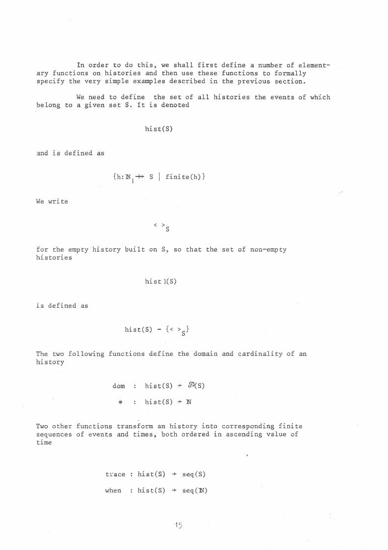
In order to do this, we shall first define a number of element­ary functions on histories and then use these functions to formally specify the very simple examples described in the previous section.

We need to define the set of all histories the events of which belong to a given set S. It is denoted

hist(S)

and 1S defined as

{h:JNj-+t- S I finite(h)}

We write

for the empty history built on S, so that the set of non-empty histories

hist I(S)

1S defined as

The two following functions define the domain and cardinality of an history

dom hist(S) + 8'J(S)

#: hi s t ( S ) + "N

Two other functions transform an history into corresponding finite sequences of events and times, both ordered in ascending value of time

trace hist(S) + seq(S)

when hist(S) + seq(JN)

15

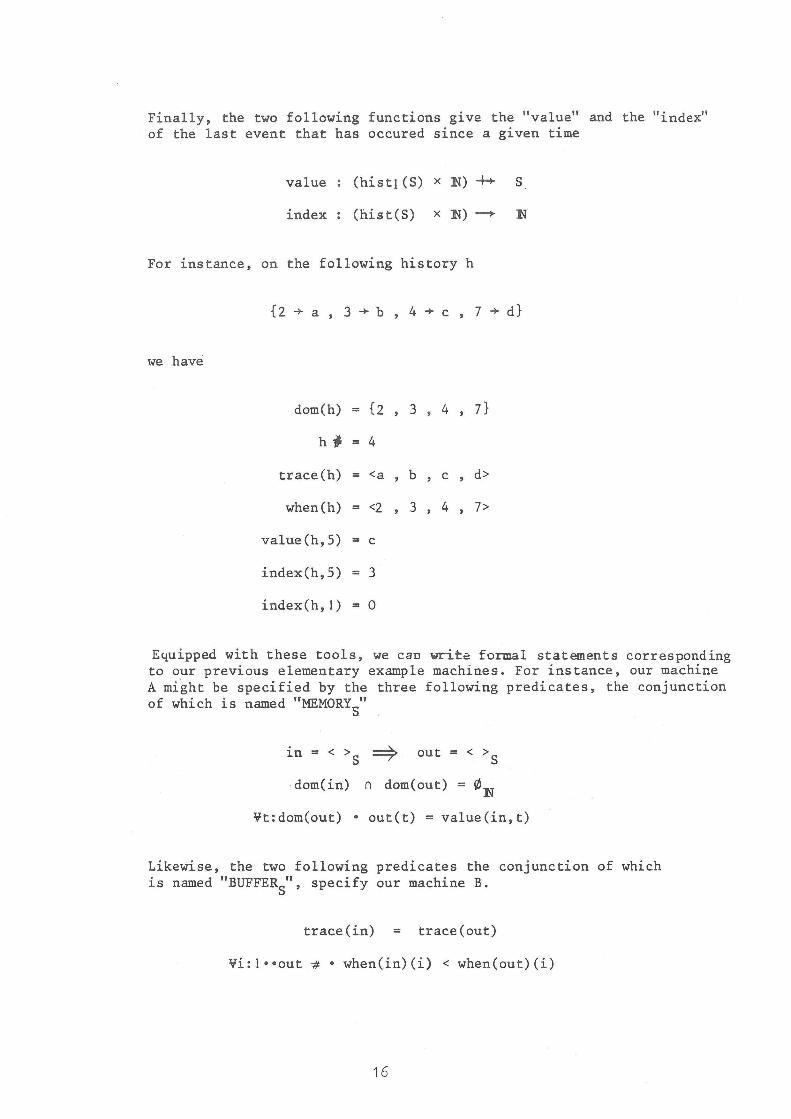
Finally, the two following functions give the "value" and the "index" of the last event that has occured since a given time

value (hisq (S) x ~) ~ S

index (hist(S) x~) - ~

For instance, on the following history h

{2 + a , 3 + b , 4 + C , 7 + d}

we have

dom(h) = {Z , 3 , 4 , 7}

hi = 4

trace(h) = <a b c d>

when (h) = <2 3 4 7>

value (h, 5) = c

index(h,5) = 3

index(h,l) = 0

Equipped with these tools, we caD write formal statements corresponding to our previous elementary example machines. For instance, our machine A might be specified by the three following predicates, the conjunction of which is named "MEMORYS"

~n = < > S ==? out = < > S

dom(in) n dom(out) = 0l\I

Vt:dom(out) • out(t) = value(in,t)

Likewise, the two following predicates the conjunction of which is named "BUFFERS", specify our machine B.

trace (in) = trace(out)

vi: 1 • ·out "# • when(in) (i) < when(out) (i)

16

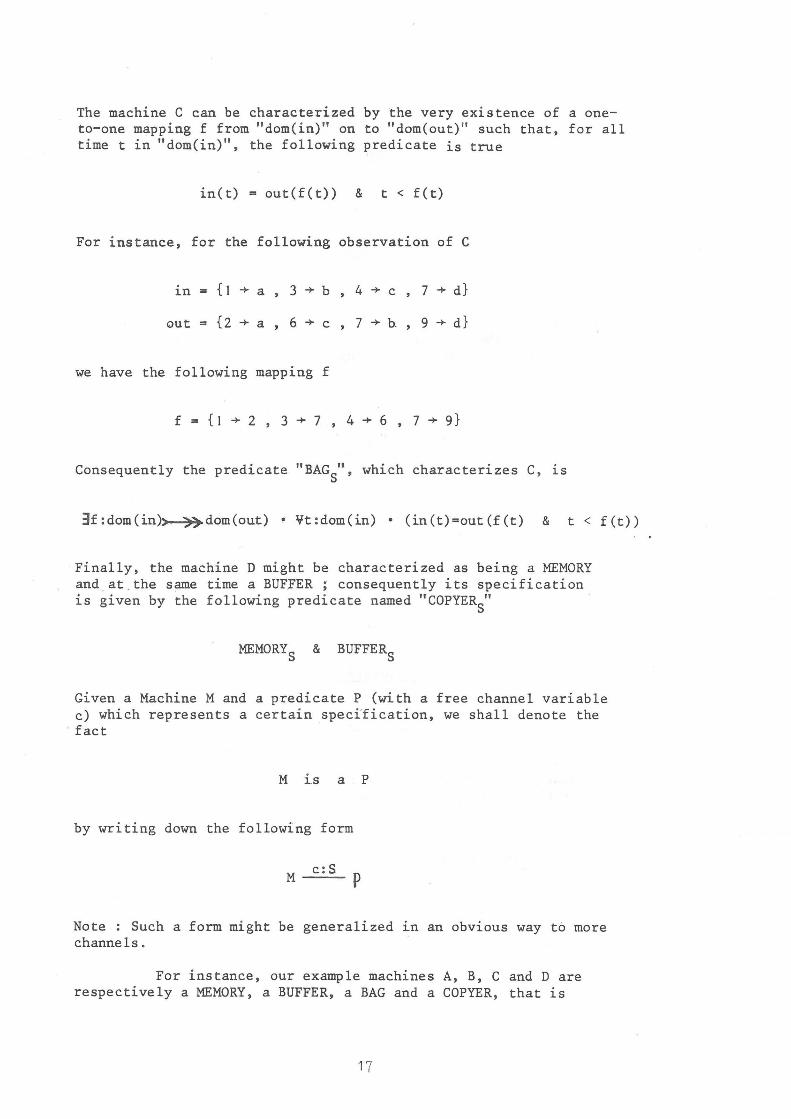
The machine C can be characterized by the very existence of a one­to-one mapping f from "dom(in)" on to "dom(out)" such that, for all time t in "dom(in)", the following predicate is true

in(t) = out(f(t» & t < f(t)

For instance, for the following observation of C

in = {I + a 3 + b 4 + C 7 + d}

out = {2 + a 6 + C 7 + b. 9 + d}

we have the following mapping f

f = {I + 2 , 3 + 7 , 4 + 6 , 7 + 9}

Consequently the predicate "BAGSIl

, which characterizes C, ~s

3f:dom(in)~dom(out) • Vt:dom(in) • (in(t)=out(f(t) & t < f(t»

Finally, the machine D might be characterized as being a MEMORY and . at the same time a BUFFER; consequently its specification is given by the following predicate named "COPYERS"

MEMORYS & BUFFERS

Given a Machine M and a predicate P (with a free channel variable c) which represents a certain specification, we shall denote the

. fact

M ~. s a P

by writing down the following form

M c:S p

Note : Such a form might be generalized ~n an obvious way to more channels.

For instance, our example machines A, B, C and Dare respectively a MEMORY, a BUFFER, a BAG and a COPYER, that is

17

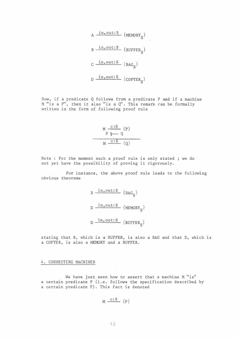
A in,out:S {MEMORYS

}

B in,out:S {BUFFERS}

C in,out:S

{BAGS}

D in,out:S {COPYER

S}

Now, if a predicate Q follows from a predicate P and if a machine M "is a P", then it also "is a Q". This remark ('.an be formally written in the form of following proof rule

M c:S {p}

P l--- Q

M c:S {Q}

Note : For the moment such a proof rule ~s only stated not yet have the possibility of proving it rigorously.

we do

For instance, the above proof rule leads to the following obvious theorems

B in,out:S {BAGS}

D in,out:S {MEMORY

S}

D in,out:S

{BUFFERS}

stating that B, which is a BUFFER, is also a BAG and that D, which ~s a COPYER, is also a MEMORY and a BUFFER.

4. CONNECTING MACHINES

We have just seen how to assert that a machine M "is" a certain predicate P (i.e. follows the specification described by a certain predicate P). This fact is denoted

M c:S {p}

13

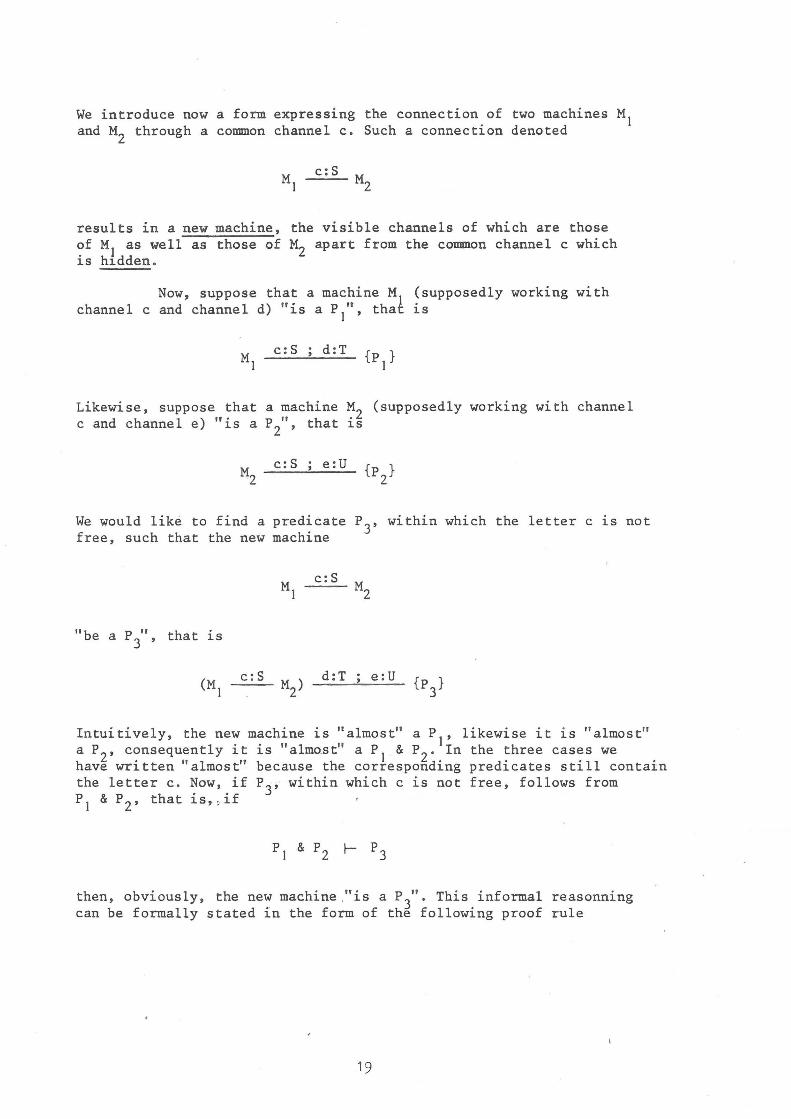
We introduce now a form expressLng the connection of two machines MI and M2 through a common channel c. Such a connection denoted

c:S

results in a new machine, the visible channels of which are those of M) as well as those of M2 apart from the common channel c which is hldden.

Now, suppose that a machine MI (supposedly working with channel c and channel d) "is a PI", that is

c:S d:T

Likewise, suppose that a machine ~2 (supposedly working with channel c and channel e) "is a P 2", that LS

c:S e:U

We would like to find a predicate P3

, within which the letter c 1S not free, such that the new machine

"be a p" th t . 3' a LS

c:S

c:S

d:T e:U

Intuitively, the new machine is "almost" a PI' likewise it is "almost" a P 2' consequently it is "almost" a PI & P 2. In the three cases we have written "almost" because the corresponding predicates still contain the letter c. Now, ifP3 , within which c is not free, follows from PI & P2 , that is, . if

then, obviously, the new machine ,"is a P3". This informal reasonning can be formally stated in the form of the following proof rule

19

MI c:S d:T

{p I}

M2 c:S e:U {P

2}

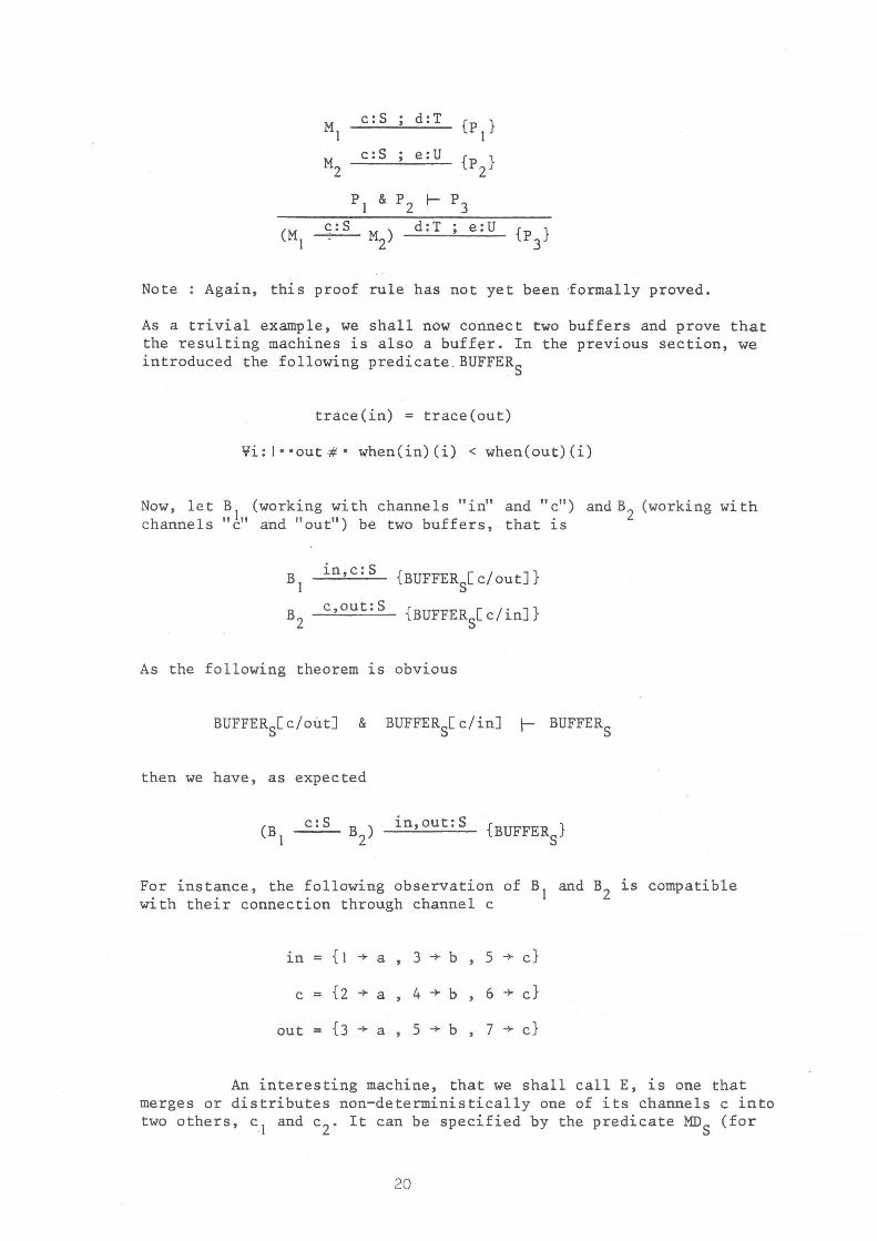
PI & P2 I- P3

(M I <;:S M2) d:T ; e:U {P

3}

Note : Again, this proof rule has not yet been formally proved.

As a trivial example, we shall now connect two buffers and prove that the resulting machines is also a buffer. In the previous section, we introduced the following predicate. BUFFERS

trace(in) = trace(out)

vi: I· ·out:#· when (in) (i) < when(out) (i)

Now, let BI (working with channels "in" and "c") andB2 (working with channels "c" and "out") be two buffers, that is

in,c:S

c,out:S

{BUFFERS[c/outJ}

{BUFFERS[c/inJ}

As the following theorem 1S obvious

BUFFERS[c/outJ & BUFFERS[c/inJ r BUFFERS

then we have, as expected

c:S in,out:S

For instance, the following observation of BI and B2 is compatible with their connection through channel c

1n = {I -+ a 3 -+ b 5 -+ c}

c = {2 -+ a 4 -+ b 6 -+ d

out = {3 -+ a 5 -+ b 7 -+ c}

An interesting machine, that we shall call E, is one that merges or distributes non-deterministically one of its channels c into two others, c

l and c2 . It can be specified by the predicate MDS (for

20

Merger-Distributor)>> which is the conjunction of the two following predicates

Note : This machine can be generalized in an obvious way so as to merge or distribute one-channel into more than two channels.

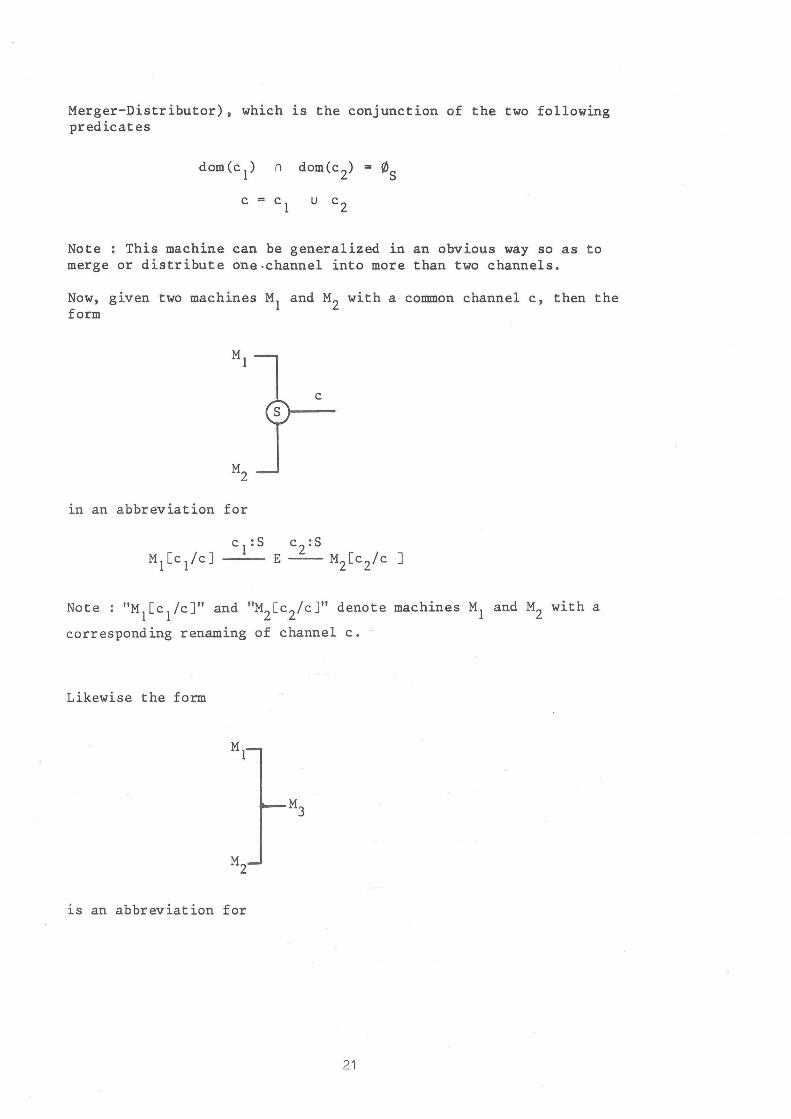
Now, given two machines Ml and MZ with a common channel c, then the form

~n an abbreviation for

Note' "M [c Ic]" and "M [c Ic]" denote machines Ml and MZ with a • 1 1 2 Z corresponding renaming of channel c.

Likewise the form

~s an abbreviation for

21

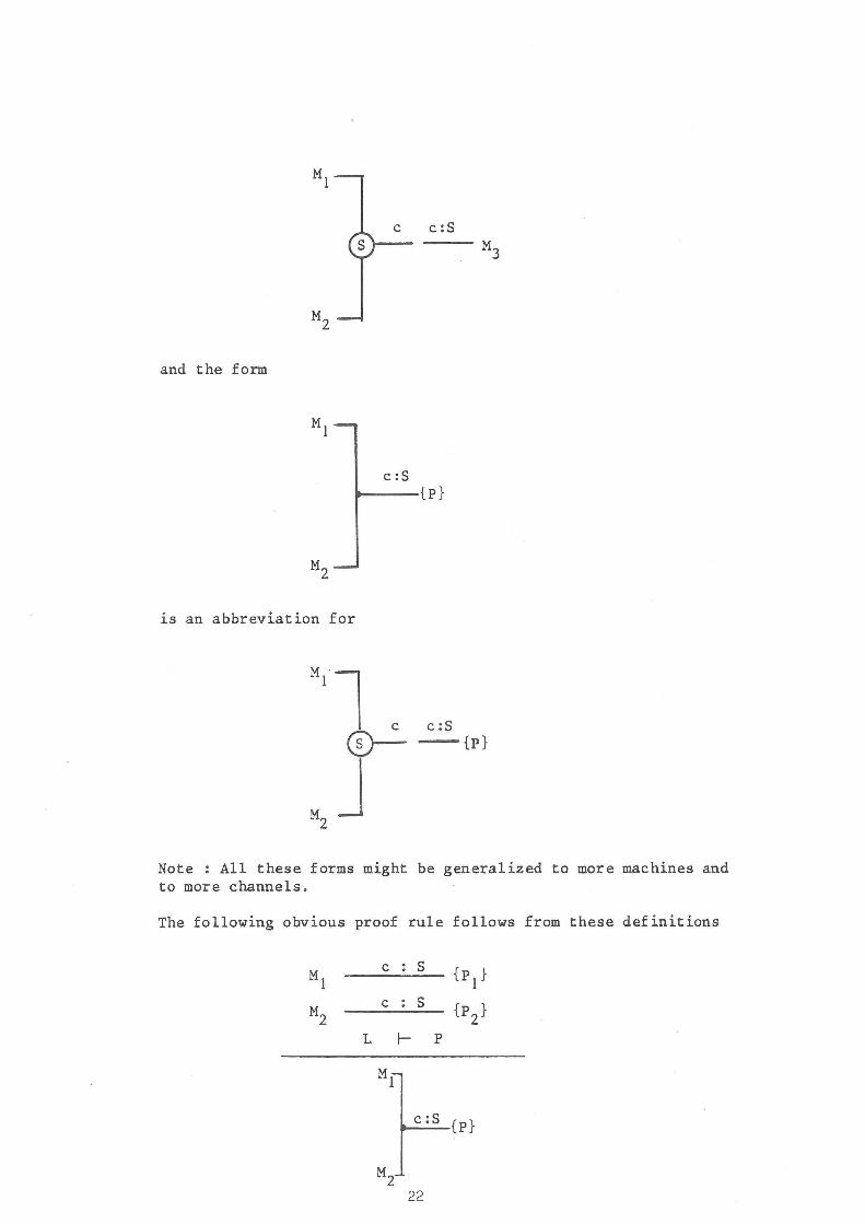
c:S

and the form

c:S -----{p}

~s an abbreviation for

c:S -{p}

Note : All these forms might be generalized to more machines and to more channels.

The following obvious proof rule follows from these definitions

MI c s

{PI}

M2 c S {P2}

L f- P

Ml

c:S {p}

M2 22

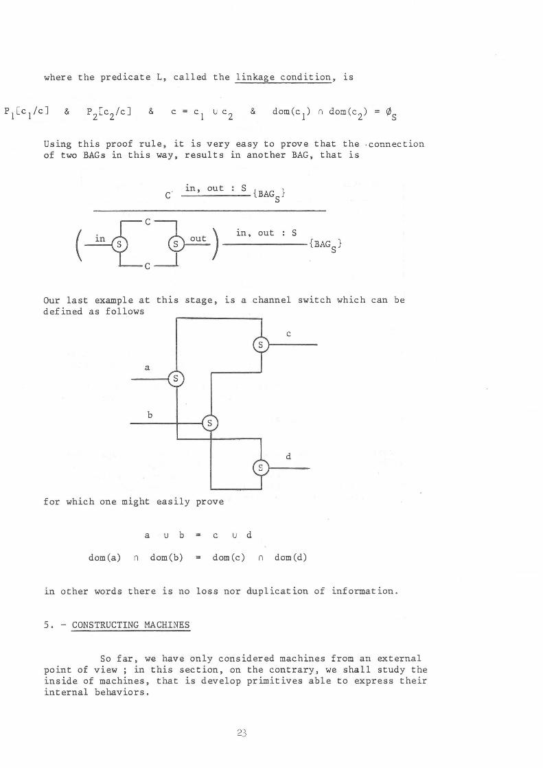
where the predicate L, called the linkage condition. ~s

& & &

Using this proof rule, it is very easy to prove that the ·connection of two BAGs in this way, results in another BAG, that is

C in, out S J }

-----1.BAGS

(~C 1 .) in, out S ~n S ~ -----{BAG

S}

c.--l·

Our last example at this stage, LS a channel switch which can be defined as follows

c

a ----{ S

b

d

for which one might easily prove

a . u b cud

dom(a) n dom(b) dom (c) n dom (d)

~n other words there ~s no loss nor duplication of information .

5. - CONSTRUCTING MACHINES

So far, we have only considered machines from an external point of view; in this section, on the contrary, we shall study the inside of machines, that is develop primitives able to express their internal behaviors.

23

Curiously enough» the number of such primitives can be re­duced to the bare minimum; in fact» we only need to express the wri­ting on or the reading from a channel» the time atomicity of an action and» finally» the starting of a machine. The following diagram shows the denotation of these operations.

Operation Denotation Notes

Reat1ing readS c (1)

Writing c ! := exp (2)

Atomici ty < p > (3)

Starting 0 (3)

Notes

(1) c denotes a history variable and S denote a set expression compatible with the carrier set of the history variable c.

(2) c denotes a history variable and "exp" denote an element expres-' sion compatible with the carrier set of the history variable c.

(3) P denotes a program.

Before defining these primitives in terms of the program features defined in the first section» we shall enlarge our previous set of tools dealing with histories. We shall define three functions yiel­ding respectively the last time» the last event and the past of a given history. These functions are the following

4- hist (5) -+ IN

? histl (5) -+ S

histl(5) -+ hist(S)

For instance» on the following history h

{I -+ a» 3 -+ b» 7 -+ c}

24

we have

h+ = 7

h? = c

h = {I ~ a, 3 ~ bI

and also, by convention

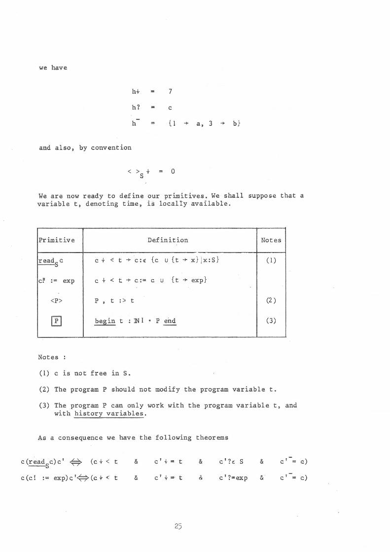
We are now ready to define our primitives. We shall suppose that a variable t, denoting time, is localry available.

Primitive Definition Notes

~Sc c + <: t ~ c:~ {c u {t ~ x} jx:S} (1)

cl' := exp c + < t ~ c:= c u {t ~ exp}

<P> P , t :> t (2 )

[!] be~in t : :IN 1 • P end (3) --

Notes

(I) c is not free 1n S.

(2) The program P should not modify the program variable t.

(3) The program P can only work with the program variable t, and with history variables.

As a consequence we have the following theorems

c (r ead S c) c' -# (c + < t

c(cl := exp)c'#(c-r < t

&

&

c'i = t

c'+=-t

25

& C'?E S

c' ?=exp

&

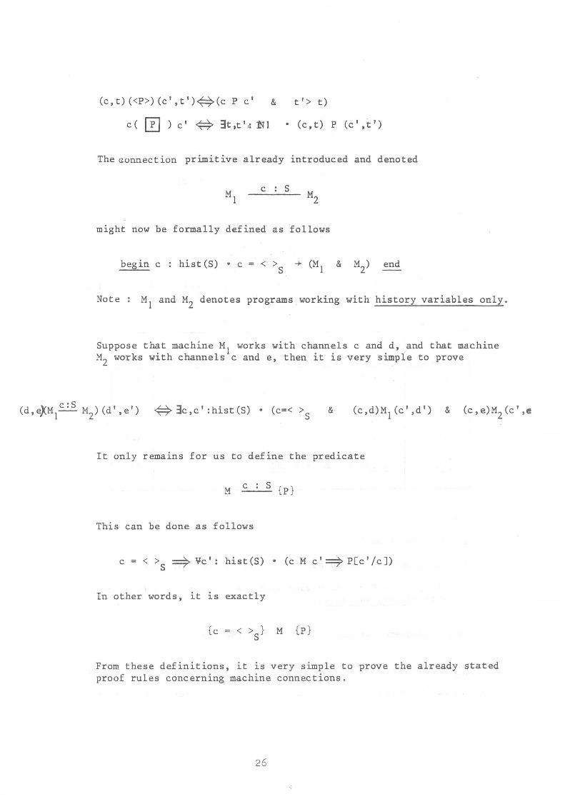
(c,t) «P» (c' ,t'){:}(c P c' & t'> t)

c( 0 ) c' # 3t,t':::lH • (c,t) P (c' ,t')

The G.onnection primitive already introduced and denoted

c : S

might now be formally def ined as follows

begin c hist (S) • c < > S

& end

Note MI and M2 denotes programs working with history variables only.

Suppose that machine MI works with channels c and d, and that machine M2 works with channels c and e, then it is very simple to prove

{:} 3c, c ' : hist (S) • (c=< > S

& (c,d)M 1 (e' ,d') & (c,e)M2

(c',e

It only remains for us to define the predicate

M _c __ S {p}

This can be done as follows

c = < >S ==? Vc': hist(S) • (c M c'==}P[c'/c])

In other words, it ~s exactly

{c < >} M {p} S

From these definitions, it is very simple to prove the already stated proof rules concerning machine connections .

26

We are also ready to construct a memory, a buffer or a copyer. Let R, Wj. and W

2 be the following programs

< readS in >

< out! := in?>

out # < in#: < out! : = trace(in) (out# +1»

Then it ~s very simple to prove

) * in, ou t S { } WI I--~----- MEMORYS '------~.-....

(R o

(R o do od ~n, out s

(R WI) * t_i_n..=.,_o_u_t __ S_ {COPYERS

}

As a copying machine is also a BAG (since it ~s a BUFFER) then we can construct a BAG as follows

* (R ; WI)

~n S S

out

* (R ; WI)

And finally our Merger/Distributor can be built from the program

c 1 »S c2

which ~s

<readS c 1 . I := c 1?> , c 2 ·

27

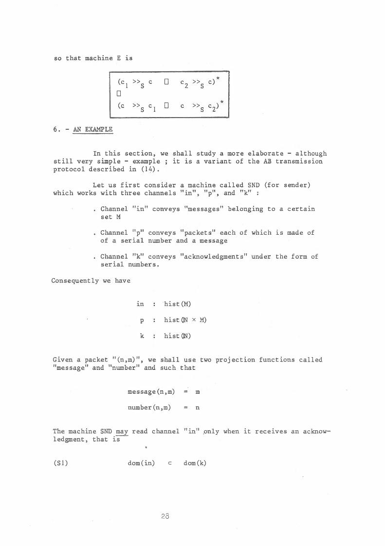
so that machine E is

(c 1 » c 0 c 2 » c)*

S S 0

(c 0 * » c1

c » c 2) S S

6. - AN EXAMPLE

In this section, we sti1l verJY simple - example protocol described in (14).

shall study a more elaborate - although it is a variant of the AB transmission

Let us first consider a machine called SND (for sender) which works with three channels "in", "p", and "k" :

Channel "in" conveys "messages" belonging to a certain set M

. Channel "p" conveys "packets" each of which ~s made of of a serial number and a message

. Channel "k" conveys "acknowledgments" under the form of serial numbers.

Consequently we have

inhist (M)

p hist (IN x M)

k hist (IN)

Given a packet "(n,m)", we shall use two projection functions called "message" and "number" and such that

message(n,m) = m

number (n,m) n

The machine SND may read channel "in" ,only when it rece1ves an acknow­ledgment, that i-s--

(SI) dom(in) c dom(k)

28

Moreover, this acknowledgment must be equal to the number of messages read so far on channel "in", that is

(S2) lit dom(in) • k(t) index (in, t-l)

The machine SND may send packets made of the last message read if any, together with the corresponding serial number, that is

(S3)

(S4)

lit

lit

dom(p) • index(in, t) # 0

dom(p) • pet) = (index(in,t), value(in,t»

Moreover 5ND must send the last message read if any, that ~s

(55) in + ~ p +

Finally, the reception of an acknowledgment and the sending of a packet excludes each other, that is

(56) dom(k) (l dom (p) =

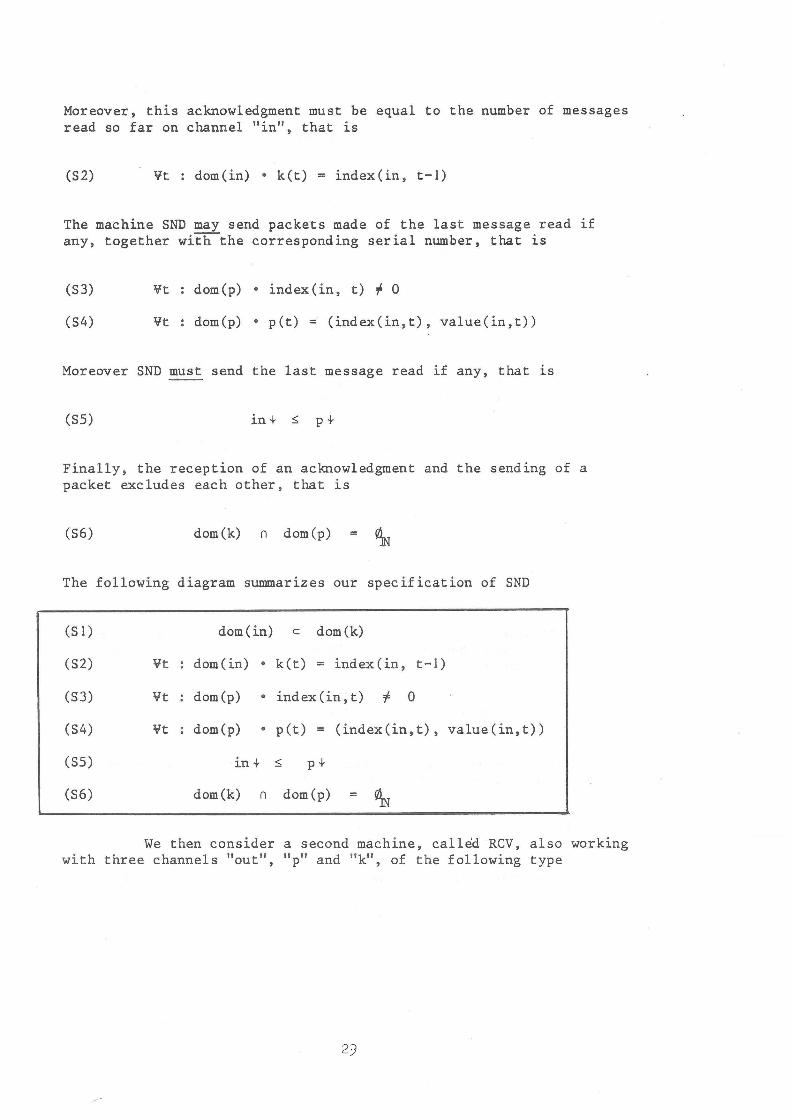
The following diagram summarizes our specification of 5ND

(51) dom(in) c dom(k)

(52) lit dom(in) • k(t) = index (in, t-l)

(53) lit dom(p) . index(in,t) # 0

(54) lit dom(p) • pet) = (index(in,t) , value (in, t»

(85) in + ~ p+

(86) dom(k) (l dom(p) = ~

We then consider a second machine, called RCV, also working with three channels "out", "p" and "k", of the following type

29

out hist (M)

p histON x M)

k hist ON)

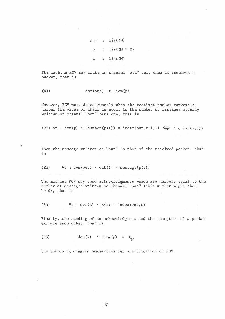
The machine Rev may write on channel "out" only when it receives a packet, that is

(RI) dom(out) c dom(p)

However, ReV must do so exactly when the received packet conveys a number the value of which is equal to the number of messages already written ori channel "out" plus one, that is

(R2) \it dom(p) • (number(p(t)) index(out,t-l)+l {:} t E dom(out))

Then the message written on "out" ~s that of the received packet, that ~s

(R3) \it dom(out) • out(t) = message(p(t)

The machine Rev may send acknowledgments which are numbers equal to the number of messages-written on channel "out" (this number might then be 0), that is

(R4) \it dom(k) • k(t) = index(out,t)

Finally,the sending of an acknowledgment and the reception of a packet exclude each other, that is

(R5) dom(k) n dom(p) =

The following diagram summar~zes our specification of RCV.

30

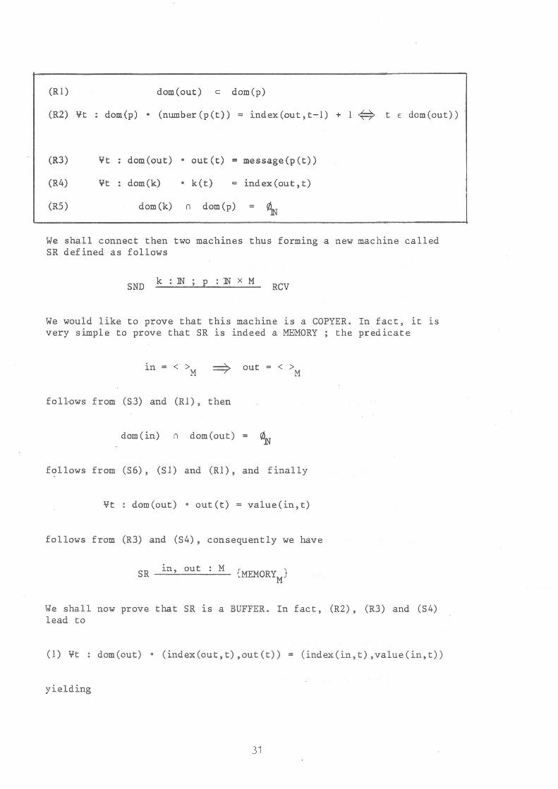
(R 1)

(R2) ¥t

(R3)

(R4)

(R5)

dom(out) c dom(p)

dom(p) • (number(p(t» = index(out,t-l) + 1 ~ t E dom(out»

¥t dom(out) out(t) = message(p(t»

¥t dom(k) • k(t) = ind ex (ou t , t)

dom(k) n dom(p)

We shall connect then two machines thus forming a new machine called SR defined as follows

SND k ::IN RCV

We would like to prove that this machine 1S a COPYER. In fact, it 1S

very simple to prove that SR is indeed a MEMORY ; the predicate

1n = < > M

out < > M

follows from (S3) and (R1), then

dom(in) n dom(out) = ~

follows from (S6), (S1) and (R1), and finally

¥t dom(out) • out(t) value(in, t)

follows from (R3) and (S4), consequently we have

SR in, out : M

We shall now prove that SR is a BUFFER. In fact, (R2) , (R3) and (S4) lead to

(1) ¥t dom(out) • (index(out,t),out(t» = (index(in,t),value(in,t»

yielding

31

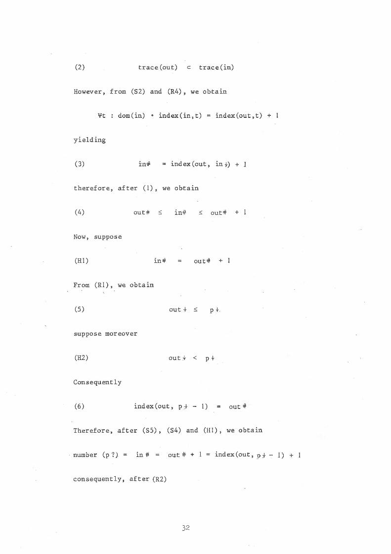
(2) trace(out) c trace(in)

However, from (S2) and (R4) , we obtain

¥t dom (in) • index (in, t) index(out,t) + 1

yielding

(3) in# = index (out, in:l-) + 1

therefore, after (1), we obtain

(4) out# ~ in# ~ out# + 1

Now, suppose

(HI) in# = out# + 1

From (Rl), we obtain

(5) out + ~ p +.

suppose moreover

(H2) out+ < P +

Consequently

(6) index (out, p j - 1) = out #

Therefore, after (S5), (S4) and (HI), we obtain

number (p?) = in# = out # + 1 = index(out,p+-l) + 1

consequently, after (R2)

32

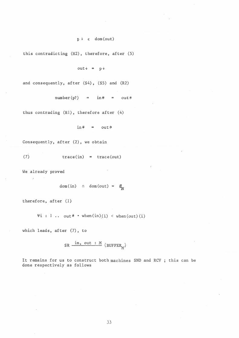
p.j.. E dom(out)

this contradicting (H2) , therefore, after (5)

out... = p +

and consequently, after (S4), (S5) and (R2)

number (p?) = in# = out#

thus contrading (HI), therefore after (4)

in# = out#

Consequently, after (2), we obtain

trace(in) = trace(out)

We already proved

dom(in) n dom(out) ~

therefore, after (1)

Vi 1.. out #: • when (in),(i) < when (out) (i)

which leads, after (7), to

SR _~n--,,=--o_u_t __ M {BUFFE~}

It remains for us to construct both machines SND and RCV done respectively as follows

33

this can be

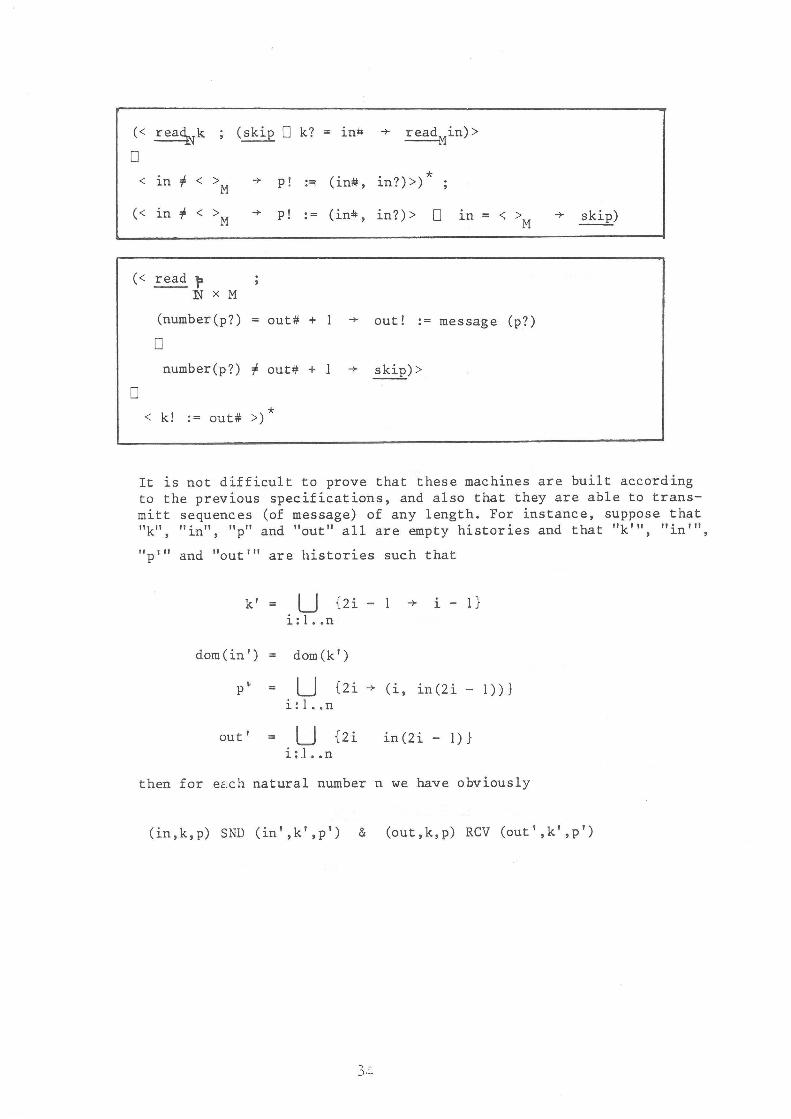
«~k (skip 0 k? in# -+ readMin)>

0

< :f < > -+ p! (in#, . ) * 1.n M

:=: l.ll? » ;

« 1.n :f < > -+ p! := (in# , in?» 0 1.n = <; > -+ skip) M M

« read ~

o

:IN x M

(number(p?)

o out# + 1 -+ out! := message (p?)

number(p?) :f out# + 1 -+ skip»

< k! * := out#: »

It is not difficult to prove that these machines are built according to the previous specifications, and also that they are able to trans­mitt sequences (of message) of any length. For instance, suppose that "k", "in", "p" and "out" all are empty histories and that "k"', "in"',

"p'" and "out'" are histories such that

k' U {2i - I -+ 1. - I} i: 1. .n

dom(in') = dom(k')

p " = U {2 i -+ ( i , in (2 i-I) ) } i: l..n

out' = U {2i i: l •• n

in(2i-l)}

then for ecLch natural number n we have obviously

(in,k,p) SND (in',k',p') & (out,k,p) Rev (out',k',p')

7. - DISTRIBUTING A PROGRAM

As a final example we shall show how one might distribute a program among several machines. The following algorithm, attributed to E.W. Dijkstra, transforms two finite and disjoint sets of Natural Numbers 51 and S2 into two other sets SI' and S2' such that

S' uS' 1 2

5 ' 1 n

max (5 1 ')

5 ' 2 =

<

In order to obtain this result one repeatealy exchanges the max~mum of 51 and the minimum of 52 until the desired condition is met.

be Let the predicate C and the programs PI and P2 respectively

<

and let the program P and the predicate A respectively be

C + (P 1 ' P 2)

51 E F 1 (E) & &

51 n S2 = ~ & = x

Note: The form Fl ON) denotes the set of non empty and finite subsets of the set of Natural Numbers N.

It is then very easy to prove the following theorems

P

do P od {A &

We shall now distribute the program

do P od

35

by "executing" both programs PI and P2 on separate communicating machines. However, before doing this, we shall define the two following functions f and g, the arguments of which are respective­ly a set (of numbers) and two sequences (of numbers) of the same size.

f , g ~ON) x seq ON) x seq ON)) + J>(JN)

We shall define these functions recursively as follows

f (S < >IN ' < > ) IN

S

g(S < >~ < > = S IN

f (S, sl~ x, s{' y) = f «S - {x}) u {y} sl s2)

g(S, s 11' x, S ~ y) = g«S u {x}) - {y} s 1 s2) 2

Note : The operator ~ denotes the "pushing" of an element at the end of a sequence.

Given two history variables M and m and two non empty finite sets of numbers SI and S2

M , m hist <N)

we define both sets S3 and S4 respectively as follows

t(SI ' trace(M) , trace(m))

g(S2 ' trace(M) , trace(m))

Let P3 and P4 be the two following programs

~m>

<~M m! := min(S4 u {M?}»

Both programs MI and M2 are now defined as follows

36

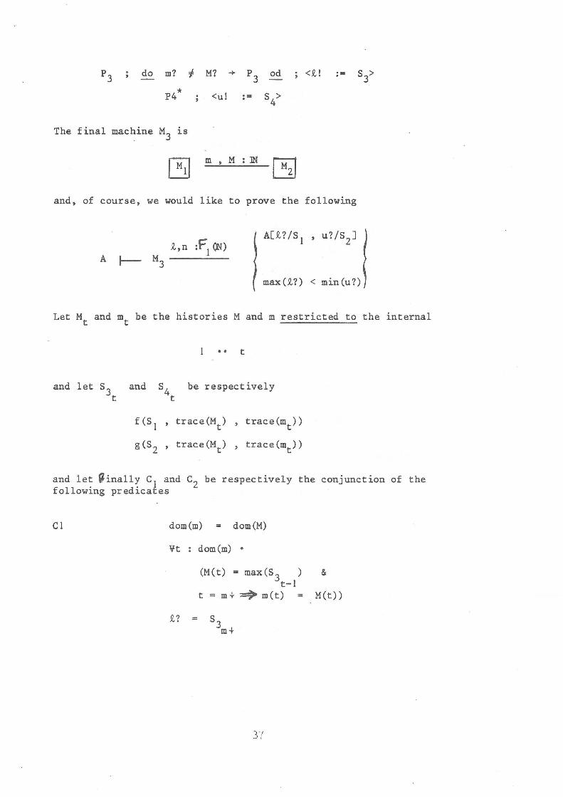
P3 do m? " M? -+ P3

od <51,! :=

P4* <u! := S4>

The final machine M3 is

BJ m , M :IN [3J and, of course, we would like to prove the following

A .Q.,n :F

1 eN)

M3 -----

S3>

max (.Q.?) < min(u?)

Let Mt and mt be the histories M and m restricted to the internal

t

and let S3 and S4 be respectively t t

f(S1 ' trace(Mt ) , trace(mt ))

g(S2 ' trace(Mt ) , trace(mt ))

and let ~inally C1 and C2 be respectively the conjunction of the following predicates

C1 dom(m) = dom(M)

lit : dom(m) •

(M ( t) = max (S 3 ) & t-1

t = m+ ~m(t) = M(t))

37

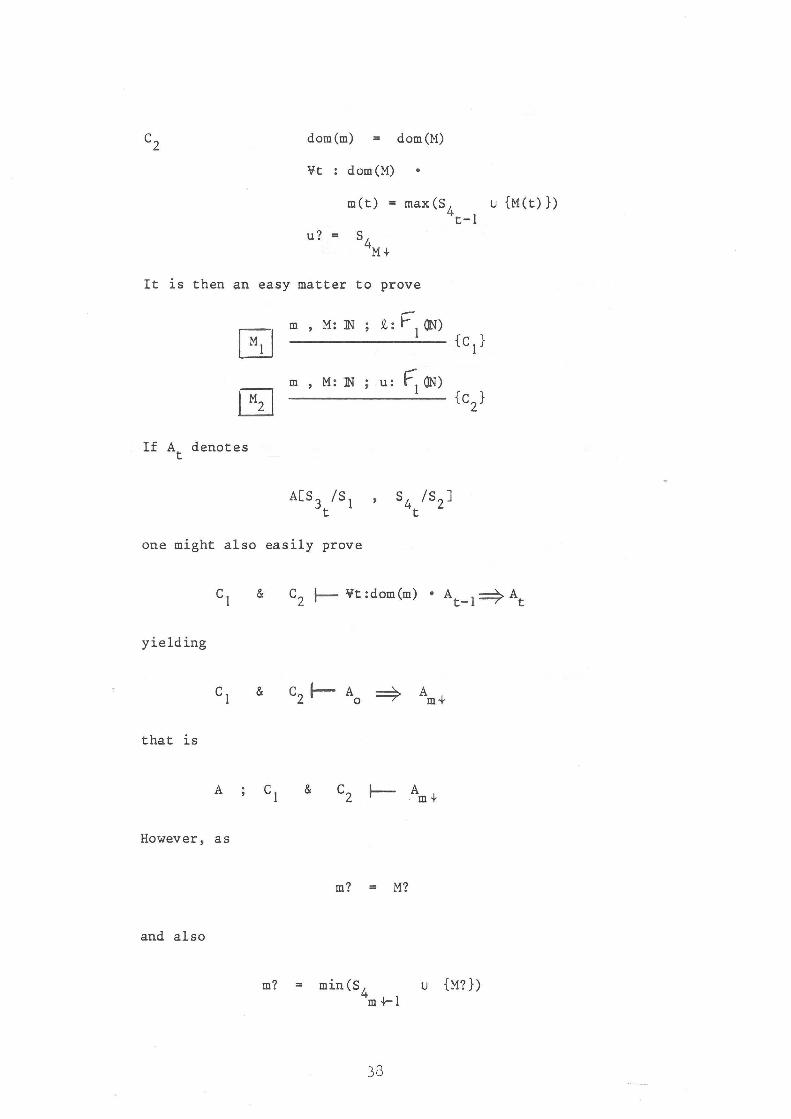
dom(m) dom(M)

lit : dom(M)

m ( t ) max (S 4 u {M ( t) } ) t-l

u?

It ~s then an easy matter to prove

5J m , M: IN ; ,Q,:F1ON)

{C1

}

5J m , M: 1N u: PION)

{C2

}

If At denotes

ACS 3 /SI t

S4 /S2 J t

one might also easily prove

&

yielding

&

that ~s

A C1 & C

2 ~ Ami-

However, as

m? = M?

and also

m? = min(S4 u {M? }) m +-1

33

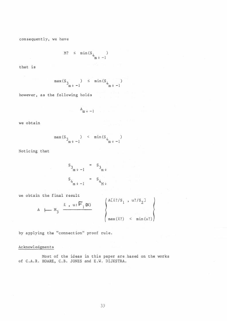
consequently, we have

M? ~ min(S4 ) m 4- -1

that ~s

max(S3 ) m 4- -1

~ min (S 4 ) m 4- -1

however, as the following holds

A m + -1

we obtain

max(S3 ) m 4- -1

< min (S 4 ) m + -1

Noticing that

we obtain the final result

max(~?) < min(u?)

by applying the "connection" proof rule.

Acknowledgments

Most of the ideas ~n this paper are.based on the works of C.A.R. HOARE, C.B. JONES and E.W. DIJKSTRA.

39

References

(1) Dijkstra A Discipline of Programming, by E.W. Dijkstra, Prentice­Hall.

(2) Hoare An axiomatic Basis for Computer Programming, by C.A.R. Hoare, CACM.

(3) Hoare : Communicating Sequential Programming, by C.A.R. Hoare, CACM, Vol. 21, nO 8, pp. 666-677.

(4) Hoare : A Non-deterministic Model for Communicating Sequential Processes, by C.A.R. Hoare, S.D. Brookes and A.W. Roscoe.

(5) Hoare : A Calculus of Total Correctness for Communicating Processes, by C.A.R. Hoare, Oxford University, PRG Monograph 23.

(6) Hoare: Specifications, Programs and Implementations, by C.A.R. Hoare, Technical Monograph PRG-29, Oxford University, June 1982.

(7) Jones : : Software Development: A Rigorous Approach, by C.B. Jones, Prentice-Hall Int. 1980.

(8) Jones : Development Methods for Computer Programs Including a Notion of Interference, by C.B. Jones, Thesis, Oxford University, 1981.

(9) Kahn : Coroutines and Network of Parallel Processes, by G. Kahn and D.B. Mac Queen in IFIP 77 Proc.

(10) Milner: An Algebraic Definition of Simulation between Programs, by R. Milner, Stanford, Memo AIM-142, Report nO CS-205.

(II) Milner: A Calculus of Communication Systems, by R. Milner, Springer Verlag, Lecture Notes in Computer Science, Vol. 92.

(12) Zhou : Partial Correctness of Communicating Sequential Processes, by Zhou Chao Chen and C.A.R. Hoare, Procs of Int. Conf. on Distri­buted Processes, Paris 1981.

(13) Zhou: Partial Correctness of Communication Protocols, by Zhou Chao Chen and C.A.R. Hoare, NPL Workshop 1981.

(14) Melliar-Smith : From state to temporal logic : specification methods for protocol standards by R.L. Schwartz and P.M. Melliar-Smith, lEE Transactions on communications, Dec. 1982.

40