spectral line observing - max planck society · 2010-09-27 essea, spectral line observing, d....
TRANSCRIPT

2010-09-27 ESSEA, Spectral Line Observing, D. Muders 1
Spectral Line Observing
Measurement goals Spectral line formation processes Line Shapes / Doppler effect Spectrometers Observing techniques Calibration Data reduction / Data products Data visualization

2010-09-27 ESSEA, Spectral Line Observing, D. Muders 2
Measurement Goals
What can we learn from radio spectral lines ? We can probe the physical, chemical and
dynamical conditions of the interstellar matter (ISM) in the Milky Way and in external galaxies.
Most ISM gas phases produce spectral lines:
Cold: 10 K, dense molecular gas (H2)
Cool: 102 K, neutral gas (HI) Warm: 104 K, ionized gas (HII) Hot: 106 K, low-density ionized (SNR bubbles)
SpectralLines

2010-09-27 ESSEA, Spectral Line Observing, D. Muders 3
Measurement Goals (ctd.)
Intensities can tell us about: Gas temperature
Energy Sources Gas density
Gravity / Cloud Criticality Chemical composition
Abundances / Evolutionary State Ionization / Magnetic Fields
Cloud Support

2010-09-27 ESSEA, Spectral Line Observing, D. Muders 4
Measurement Goals (ctd.)
Frequencies and line widths can be used to derive: Dynamical models
Galaxy and Cloud Rotation Cloud Collapse Protostellar Outflows
Redshifts Age Distance

2010-09-27 ESSEA, Spectral Line Observing, D. Muders 5
Spectroscopy
Spectroscopy:
Any measurement of a quantity as a function of either wavelength (λ) or frequency (ν), i.e. also of energy (E = hν). Spectral Line:
Result of the interaction between a quantum system and a single photon.

2010-09-27 ESSEA, Spectral Line Observing, D. Muders 6
How do spectral lines form ?
Quantum systems (atoms or molecules) can change their states only in discrete amounts of energy ΔE
The transition between these states leads to emission or absorption of light at a single frequency ν = ΔE/h, the so called rest frequency
Spectrally this transition is seen as a line

2010-09-27 ESSEA, Spectral Line Observing, D. Muders 7
Types of Spectra
http://www.astro.columbia.edu/~archung/labs/fall2001/lec04_fall01.html

2010-09-27 ESSEA, Spectral Line Observing, D. Muders 8
Types of Spectra
http://www.astro.columbia.edu/~archung/labs/fall2001/lec04_fall01.html

2010-09-27 ESSEA, Spectral Line Observing, D. Muders 9
Types of Spectra
http://www.astro.columbia.edu/~archung/labs/fall2001/lec04_fall01.html

2010-09-27 ESSEA, Spectral Line Observing, D. Muders 10
Atomic Lines I
Electronic transitions (e.g. recombination lines (H<n>α, etc.))

2010-09-27 ESSEA, Spectral Line Observing, D. Muders 11
Atomic Lines II
Hyperfine splitting / spin flips (e.g. HI 21 cm line → separate talk on Tuesday)

2010-09-27 ESSEA, Spectral Line Observing, D. Muders 12
Molecular Lines I
Electronic transitions (rather in VIS / UV) Rotational
transitions (needs
dipole, so no H2 !)
Vibrational
transitions
Animations: http://www.shokabo.co.jp/sp_e/optical/labo/opt_line/opt_line.htm

2010-09-27 ESSEA, Spectral Line Observing, D. Muders 13
Molecular Lines I
Animations: http://www.shokabo.co.jp/sp_e/optical/labo/opt_line/opt_line.htm

2010-09-27 ESSEA, Spectral Line Observing, D. Muders 14
Molecular Lines II
InversionHere: Nitrogen tunnels through double well potential
Hyperfine splitting
NH3

2010-09-27 ESSEA, Spectral Line Observing, D. Muders 15
Molecular Lines II
Inversion
Hyperfine splitting
NH3

2010-09-27 ESSEA, Spectral Line Observing, D. Muders 16
Interstellar Fingerprints
Set of all possible lines of an atom or molecule is its personal “fingerprint”
Schilke et al. ApJS 108:301–337, 1997

2010-09-27 ESSEA, Spectral Line Observing, D. Muders 17
Interstellar Molecular Zoo
www.cdms.de 08/2010

2010-09-27 ESSEA, Spectral Line Observing, D. Muders 18
Interstellar Molecular Zoo
www.cdms.de 08/2010
1
3334
9109
1618
23
3335
Total of 164 and counting !
Ethyl formateBelloche et al. A&A, 499, 215, 2009

2010-09-27 ESSEA, Spectral Line Observing, D. Muders 19
Spectral Line Excitation
Near HII regions radiatively via UV fields In cold molecular clouds via CMB but
predominantly via collisions with H2
In case of a level inversion one gets a maser (→ see also special maser talk tomorrow)

2010-09-27 ESSEA, Spectral Line Observing, D. Muders 20
Collisional Excitation
http://dsnra.jpl.nasa.gov/IMS/

2010-09-27 ESSEA, Spectral Line Observing, D. Muders 21
Maser Molecules
http://www.daviddarling.info/encyclopedia/I/interstellar_maser.html

2010-09-27 ESSEA, Spectral Line Observing, D. Muders 22
Zeeman Effect
Degenerate energy levels split up if an external magnetic field is applied
This leads to additional transitions and allows to measure the magnetic field
Kingshuk Majumdar (2000)

2010-09-27 ESSEA, Spectral Line Observing, D. Muders 23
Optical Depth Effects
Depending on the density and temperature spectral line emission can be optically thin or thick
In the case of optical depth τ « 1, one can look through a cloud and determine column densities and internal dynamics
For τ » 1, one can see only the surface of an object. Using radiative transfer one can calculate the cloud temperature

2010-09-27 ESSEA, Spectral Line Observing, D. Muders 24
Line Profile Shape
Ideal line should be infinitely sharp because there is a fixed energy difference ΔE = hν
0
Energy uncertainty causes a small broadening, the “natural line width”
Thermal motion of emitters leads to Doppler shifted line frequencies

2010-09-27 ESSEA, Spectral Line Observing, D. Muders 25
Thermal Broadening
Considering statistical ensembles one can derive a Gaussian shape for the broadened line
Only the line-of-sight, i.e. the radial component adds to this effect

2010-09-27 ESSEA, Spectral Line Observing, D. Muders 26
Radial Velocity
Larger Doppler shifts can occur due to several effects: Galactic rotation Dynamical processes in molecular clouds and stars Expansion of the universe (redshift can be so large
that submm lines are shifted to cm wavelengths !)
Each type of shift creates typical line profile shapes
We often use radial Doppler velocity as x-axis

2010-09-27 ESSEA, Spectral Line Observing, D. Muders 27
Dynamics: Rotation

2010-09-27 ESSEA, Spectral Line Observing, D. Muders 28
Dynamics: Cloud Collapse
Neal J. Evans II, ARAA, 37, 311, 1999http://www.oglethorpe.edu/faculty/~m_rulison

2010-09-27 ESSEA, Spectral Line Observing, D. Muders 29
Dynamics: Outflows
Schmid-Burgk et al. ApJ 362L, 25, 1990 Schmid-Burgk et al. LIACo, 29, 193, 1990

2010-09-27 ESSEA, Spectral Line Observing, D. Muders 30
Spectral Instruments
What does one need to observe radio astronomical spectral lines ? Heterodyne frontend (→ special talk) Usually a down-converter from observing
frequencies to a “low” (0-4 GHz) intermediate frequency (IF) band
Spectrometers to analyze the signal
Will concentrate on spectrometers here

2010-09-27 ESSEA, Spectral Line Observing, D. Muders 31
Spectrometers
Spectrometers measure the frontend signal in many frequency bins across the available bandwidth
There are several techniques: Filter banks: Series of analog filters; complex
electronics Auto-correlators: Special purpose computers;
correlation function of time series signals; low number of bits

2010-09-27 ESSEA, Spectral Line Observing, D. Muders 32
Spectrometers (ctd.)
More spectrometer types Acousto-optical spectrometers (AOS): Diffraction of
laser light at ultrasonic waves in a Bragg crystal; delicate optical setup
Fast Fourier Transform Spectrometers: High speed ADCs and FPGAs → Development at the MPIfR

2010-09-27 ESSEA, Spectral Line Observing, D. Muders 33
Fast Fourier Transform Spectrometer
XFFTS: 2.5 GHz bandwidth / 32768 channels (ENBW 88.5 kHz)
E2V 5 GS/s 10-bit ADC, XILINX Virtex-6 LX240T[ 40 nm, 1.0 volt core voltage, >240‘000 logic cells, 768 DSP48 slices ]

2010-09-27 ESSEA, Spectral Line Observing, D. Muders 34
Observations
Source signal is partially absorbed by the earth atmosphere
The atmosphere also radiates itself and thus contributes to the signal

2010-09-27 ESSEA, Spectral Line Observing, D. Muders 35
Atmospheric Transmission

2010-09-27 ESSEA, Spectral Line Observing, D. Muders 36
Observations
Source signal is partially absorbed by the earth atmosphere
The atmosphere also radiates itself and thus contributes to the signal
The telescope beam picks up ground spillover Receiver etc. add a signal too Direct measurement therefore yields
Con
= Csource
e-τA + Catm
(1-e-τA) + Cspillover
+ Crec

2010-09-27 ESSEA, Spectral Line Observing, D. Muders 37
On-Off Technique
To remove the atmospheric and instrumental emissions one observes the target and then a position on sky without astronomical emission
Coff
= Catm
(1-e-τA) + Cspillover
+ Crec
The difference of the two measurements contains only the source signal (still weakened by atmospheric absorption):
Con
- Coff
= Csource
e-τA

2010-09-27 ESSEA, Spectral Line Observing, D. Muders 38
On-Off Technique
Source signal plus atmosphereand receiver / amplifiers

2010-09-27 ESSEA, Spectral Line Observing, D. Muders 39
On-Off Technique
Reference signal plus atmosphereand receiver / amplifiers

2010-09-27 ESSEA, Spectral Line Observing, D. Muders 40
On-Off Technique
Source minus Reference

2010-09-27 ESSEA, Spectral Line Observing, D. Muders 41
On-Off Technique
Source minus Reference Reference

2010-09-27 ESSEA, Spectral Line Observing, D. Muders 42
On-Off Alternatives
On-Off measurements can be taken by moving the telescope between two positions.
If the source is small, then one can use horn or wobbler switching which is faster. This helps if the atmospheric emission varies quickly.
One can also measure the “off” at a slightly shifted frequency but pointing to the source. This doubles the actual “on” time and reduces telescope movements.

2010-09-27 ESSEA, Spectral Line Observing, D. Muders 43
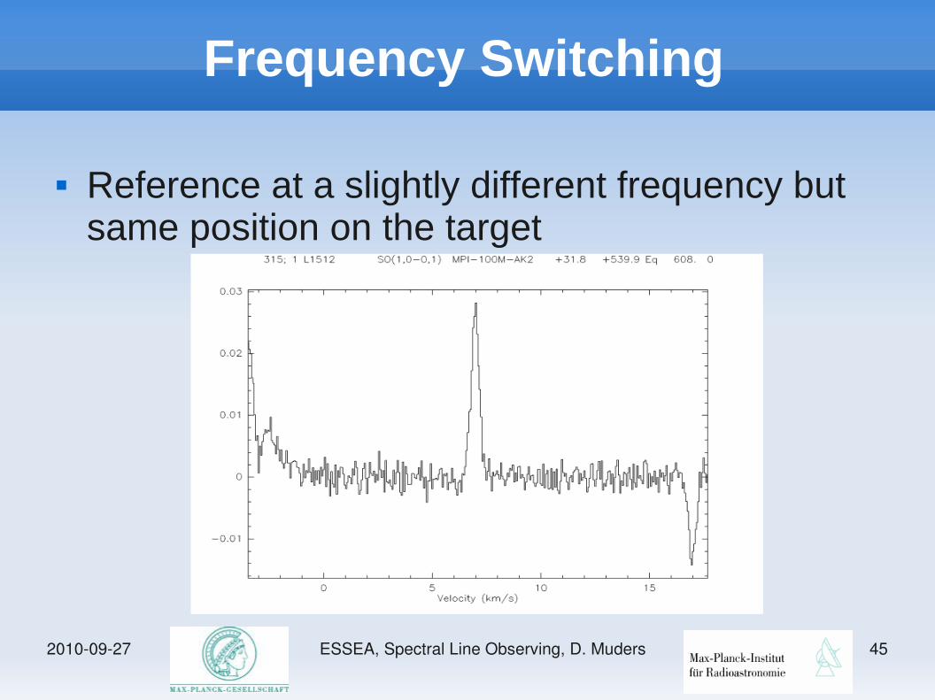
Frequency Switching
Reference at a slightly different frequency but same position on the target

2010-09-27 ESSEA, Spectral Line Observing, D. Muders 44
Frequency Switching
Reference at a slightly different frequency but same position on the target
2010-09-27 ESSEA, Spectral Line Observing, D. Muders 45
Frequency Switching
Reference at a slightly different frequency but same position on the target

2010-09-27 ESSEA, Spectral Line Observing, D. Muders 46
Observing Patterns
Most radio receivers are still single pixel or small multi-beam systems
To cover an extended source area one must observe several spatial offset positions
Typical patterns are (Rectangular) rasters with half beam spacing (Rectangular) “On-The-Fly” rasters Advanced figures like spirals, Lissajous figures,
Rotating bow ties, etc.

2010-09-27 ESSEA, Spectral Line Observing, D. Muders 47
Observing Patterns
Most radio receivers are still single pixel or small multi-beam systems
To cover an extended source area one must observe several spatial offset positions
Typical patterns are (Rectangular) rasters with half beam spacing (Rectangular) “On-The-Fly” rasters Advanced figures like spirals, Lissajous figures,
Rotating bow ties, etc.
L1512, SO 1-0, 100m

2010-09-27 ESSEA, Spectral Line Observing, D. Muders 48
Calibration
The measurements in arbitrary counts need to be calibrated to physical units
For spectral lines one usually uses the “Antenna Temperature” scale
The receiver system is calibrated against “hot” (usually ambient temperature) and “cold” (usually LN
2 @ 77 K) black bodies
In cm wave receivers one uses a noise diode that was hot/cold calibrated in the lab

2010-09-27 ESSEA, Spectral Line Observing, D. Muders 49
Calibration (ctd.)
The absorption of astronomical signals needs to be corrected too: Scaling according to measurements of secondary
calibrator sources Sky measurements and atmospheric models can be
used to derive τ More details in the calibration talk on Thursday

2010-09-27 ESSEA, Spectral Line Observing, D. Muders 50
Data reduction
Atmospheric and instrumental instabilities lead to spectral baseline artifacts

2010-09-27 ESSEA, Spectral Line Observing, D. Muders 51
Data reduction

2010-09-27 ESSEA, Spectral Line Observing, D. Muders 52
Data reduction
Atmospheric and instrumental instabilities lead to spectral baseline artifacts
Techniques to process spectral line data include: Spectral baseline fits using polynomials FFT analysis to remove sinusoidal components due
to standing waves Flagging of very bad data
Caveat: Must be very careful not to alter the line emission, esp. for broad lines

2010-09-27 ESSEA, Spectral Line Observing, D. Muders 53
Data Products
Primary data products are calibrated spectra For mapping projects the spatially distributed
spectra are interpolated onto a regular grid to make 3D data cubes with two spatial and one spectral axis
ALMA Pipeline Heuristics development (led by MPIfR) attempts to provide automatic data reduction (also applicable to Effelsberg data)

2010-09-27 ESSEA, Spectral Line Observing, D. Muders 54
Spectral Data Visualization
Usually display maps as false color images and contour plots
Frequency axis allows for additional analysis, e.g. via so called channel maps or via position-velocity plots
Since we have a data cube, one can apply 3D rendering techniques but one must be careful interpreting the graphs because of the frequency axis

2010-09-27 ESSEA, Spectral Line Observing, D. Muders 55
Channel Maps
L1512, SO 1-030 GHzEffelsberg 100m

2010-09-27 ESSEA, Spectral Line Observing, D. Muders 56
Position Velocity Plots
Plot spatial axis against velocity to study cloud dynamics, e.g. Keplerian rotation
Gomez's Hamburger (IRAS 18059-3211)
Buj
arr
abal
et
al. A
&A
483
, 83
9-84
5, 2
008
A. Gomez, CTIO, NOAO, HST, NASA
CO 2-1

2010-09-27 ESSEA, Spectral Line Observing, D. Muders 57
3D Rendering
http://am.iic.harvard.edu

2010-09-27 ESSEA, Spectral Line Observing, D. Muders 58
3D Rendering
http://am.iic.harvard.edu

2010-09-27 ESSEA, Spectral Line Observing, D. Muders 59
Deriving Physical Parameters
Spectra and data cubes of several transitions are used in conjunction with models to derive physical parameter of the ISM: Optically thin lines (involving isotopologues) to
calculate column and volume densities Line Ratios are modeled with chemical networks
and radiative transfer programs Spectral signatures of dynamical processes are
fitted against the data And many more ...

2010-09-27 ESSEA, Spectral Line Observing, D. Muders 60
Summary
Spectral lines provide a wealth of information about the interstellar medium
Different atomic and molecular processes generate numerous spectral lines in the cm to submm wavelength range
More than 160 molecules detected in space Physical, chemical and dynamical state of
interstellar medium can be studied using spectral lines

2010-09-27 ESSEA, Spectral Line Observing, D. Muders 61
Happy Observing !

2010-09-27 ESSEA, Spectral Line Observing, D. Muders 62
Thermal Line Broadening
http://hyperphysics.phy-astr.gsu.edu/hbase/atomic/broaden.html

2010-09-27 ESSEA, Spectral Line Observing, D. Muders 63
Antenna Temperature
Antenna temperature is a measure of signal strength in radio astronomy. It is defined asthe temperature of a black-body enclosure which, if completely surrounding a radiotelescope, would produce the same signal power as the source under observation.Antenna temperature is a property of the source, not of the antenna itself.
R(Θ,Φ) is the antenna pattern.