speech processing speech coding. 7 october 2015veton këpuska2 speech coding definition: speech...
TRANSCRIPT
Speech Processing
Speech Coding
April 19, 2023 Veton Këpuska 2
Speech Coding Definition:
Speech Coding is a process that leads to the representation of analog waveforms with sequences of binary digits.
Even though availability of high-bandwidth communication channels has increased, speech coding for bit reduction has retained its importance. Reduced bit-rates transmissions required for cellular networks Voice over IP
Coded speech Is less sensitive than analog signals to transmission noise Easier to:
protect against (bit) errors Encrypt Multiplex, and Packetize
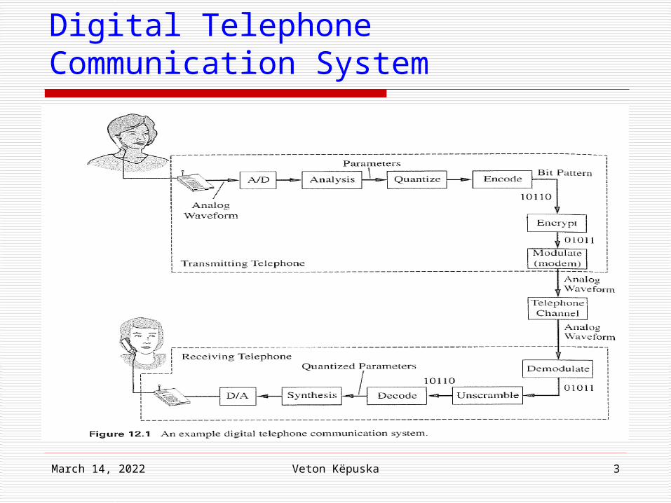
Typical Scenario depicted in next slide (Figure 12.1)
April 19, 2023 Veton Këpuska 3
Digital Telephone Communication System
April 19, 2023 Veton Këpuska 4
Categorization of Speech Coders
Waveform Coders: Used to quantize speech samples directly and
operate at high-bit rates in the range of 16-64 kbps (bps - bits per second)
Hybrid Coders Are partially waveform coders and partly speech
model-based coders and operate in the mid bit rate range of 2.4-16 kbps.
Vocoders Largely model-based and operate at a low bit
rate range of 1.2-4.8 kbps. Tend to be of lower quality than waveform and
hybrid coders.
April 19, 2023 Veton Këpuska 5
Quality Measurements
Quality of coding can is viewed as the closeness of the processed speech to the original speech or some other desired speech waveform. Naturalness Degree of background artifacts Intelligibility Speaker identifiability Etc.
April 19, 2023 Veton Këpuska 6
Quality Measurements
Subjective Measurement: Diagnostic Rhyme Test (DRT) measures
intelligibility. Diagnostic Acceptability Measure and
Mean Opinion Score (MOS) test provide a more complete quality judgment.
Objective Measurement: Segmental Signal to Noise Ratio (SNR) –
average SNR over a short-time segments Articulation Index – relies on an average SNR
across frequency bands.
April 19, 2023 Veton Këpuska 7
Quality Measurements
A more complete list and definition of subjective and objective measures can be found at: J.R. Deller, J.G. Proakis, and J.H.I Hansen,
“Discrete-Time Processing of Speech”, Macmillan Publishing Co., New York, NY, 1993
S.R. Quackenbush, T.P. Barnwell, and M.A. Clements, “Objective Measures of Speech Quality. Prentice Hall, Englewood Cliffs, NJ. 1988
Statistical Models
April 19, 2023 Veton Këpuska 9
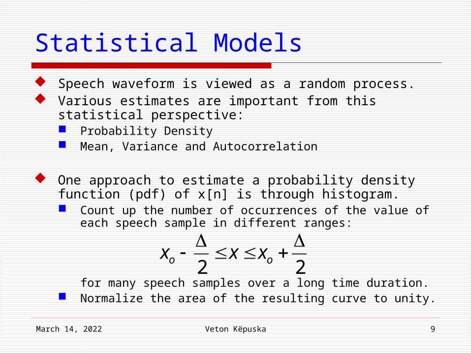
Statistical Models Speech waveform is viewed as a random process. Various estimates are important from this statistical
perspective: Probability Density Mean, Variance and Autocorrelation
One approach to estimate a probability density function (pdf) of x[n] is through histogram. Count up the number of occurrences of the value of each
speech sample in different ranges:
for many speech samples over a long time duration. Normalize the area of the resulting curve to unity.
22
oo xxx
April 19, 2023 Veton Këpuska 10
Statistical Models
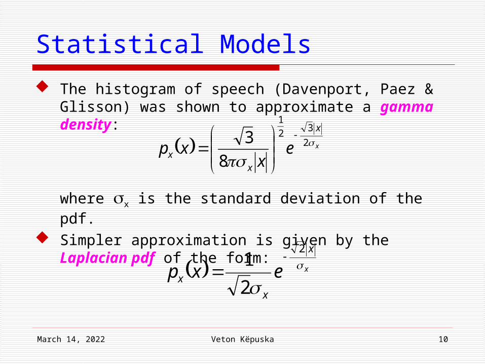
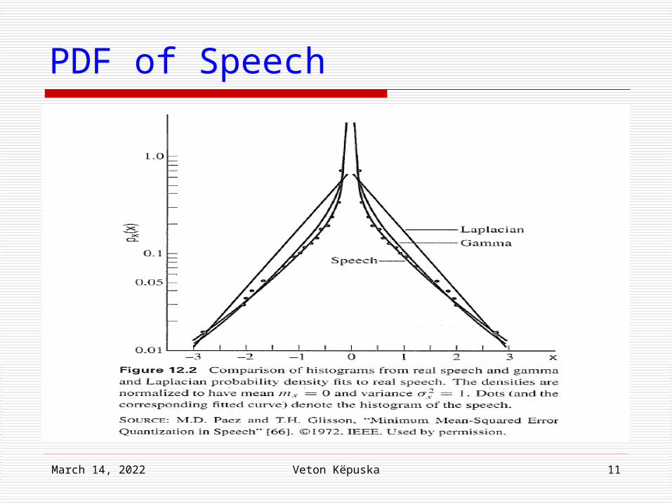
The histogram of speech (Davenport, Paez & Glisson) was shown to approximate a gamma density:
where x is the standard deviation of the pdf. Simpler approximation is given by the Laplacian
pdf of the form:
x
x
xx e
xxp
2
32
1
8
3
x
x
x
x exp
2
2
1
April 19, 2023 Veton Këpuska 11
PDF of Speech
April 19, 2023 Veton Këpuska 12
PDF of Modeled Speech
April 19, 2023 Veton Këpuska 13
PDF of Speech
Knowing pdf of speech is essential in order to optimize the quantization process of analog/continous valued samples.
Quantization of Speech & Audio Signals
Scalar QuantizationVector Quantization
April 19, 2023 Veton Këpuska 15
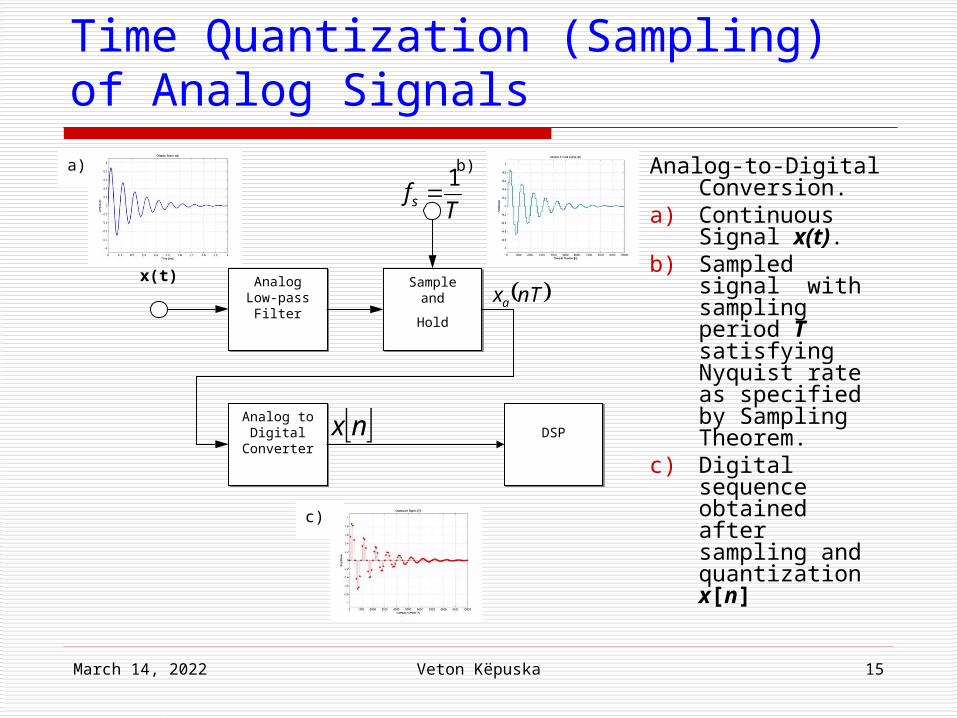
Time Quantization (Sampling) of Analog Signals
Analog-to-Digital Conversion.
a) Continuous Signal x(t).
b) Sampled signal with sampling period T satisfying Nyquist rate as specified by Sampling Theorem.
c) Digital sequence obtained after sampling and quantization x[n]
a)
x(t) AnalogLow-pass
Filter
AnalogLow-pass
Filter
Sampleand
Hold
Sampleand
Hold
b)
Analog to Digital
Converter
Analog to Digital
ConverterDSPDSP
c)
Tfs
1
nTxa
nx
April 19, 2023 Veton Këpuska 16
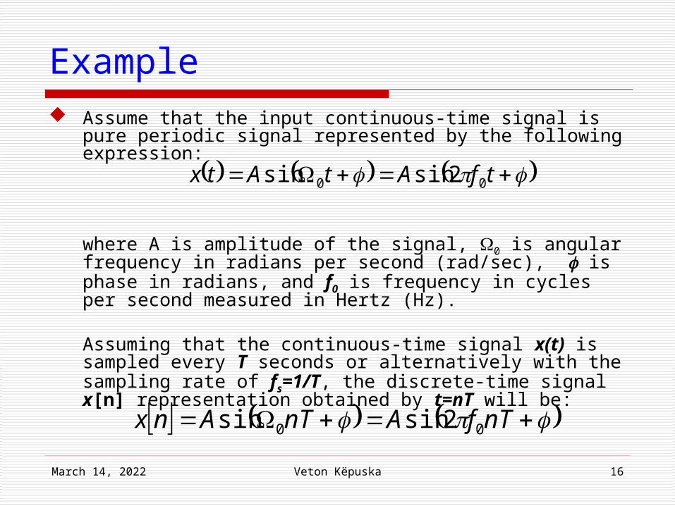
Example Assume that the input continuous-time signal is pure
periodic signal represented by the following expression:
where A is amplitude of the signal, 0 is angular frequency in radians per second (rad/sec), is phase in radians, and f0 is frequency in cycles per second measured in Hertz (Hz).
Assuming that the continuous-time signal x(t) is sampled every T seconds or alternatively with the sampling rate of fs=1/T, the discrete-time signal x[n] representation obtained by t=nT will be:
tfAtAtx 00 2sinsin
nTfAnTAnx 00 2sinsin
April 19, 2023 Veton Këpuska 17
Example (cont.)
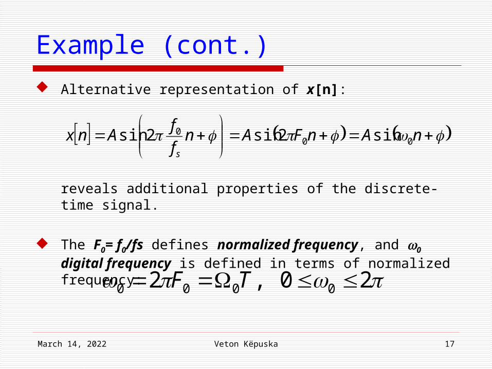
Alternative representation of x[n]:
reveals additional properties of the discrete-time signal.
The F0= f0/fs defines normalized frequency, and 0 digital frequency is defined in terms of normalized frequency:
nAnFAn
f
fAnx
s00
0 sin2sin2sin
20,2 0000 TF
April 19, 2023 Veton Këpuska 18
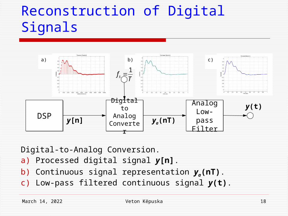
Reconstruction of Digital Signals
Digital-to-Analog Conversion. a) Processed digital signal y[n]. b) Continuous signal representation ya(nT). c) Low-pass filtered continuous signal y(t).
DSPDSPDigital toAnalog
Converter
Digital toAnalog
Converter
AnalogLow-pass
Filter
AnalogLow-pass
Filtery[n] ya(nT)
c)b)a)
y(t)
Tfs
1
Scalar Quantization
April 19, 2023 Veton Këpuska 20
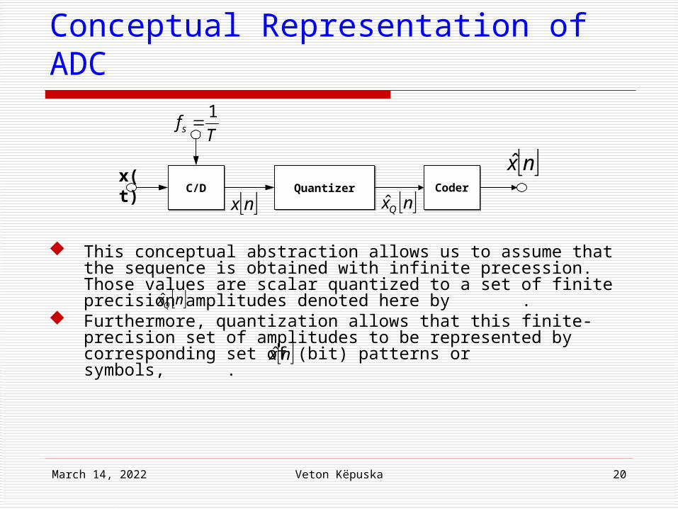
Conceptual Representation of ADC
Tfs
1
This conceptual abstraction allows us to assume that the sequence is obtained with infinite precession. Those values are scalar quantized to a set of finite precision amplitudes denoted here by .
Furthermore, quantization allows that this finite-precision set of amplitudes to be represented by corresponding set of (bit) patterns or symbols, .
x(t)C/DC/D QuantizerQuantizer CoderCoder
nx nxQˆ
nx̂
nxQˆ
nx̂
Tfs
1
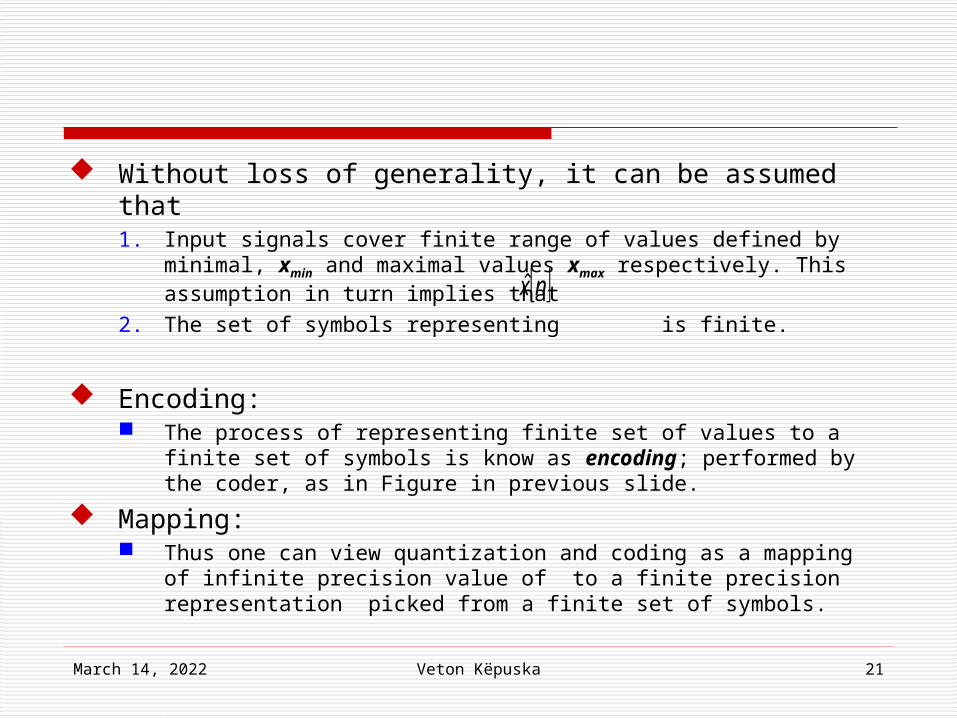
Without loss of generality, it can be assumed that 1. Input signals cover finite range of values defined by minimal, xmin
and maximal values xmax respectively. This assumption in turn implies that
2. The set of symbols representing is finite.
Encoding: The process of representing finite set of values to a finite set of
symbols is know as encoding; performed by the coder, as in Figure in previous slide.
Mapping: Thus one can view quantization and coding as a mapping of infinite
precision value of to a finite precision representation picked from a finite set of symbols.
April 19, 2023 Veton Këpuska 21
nx̂
April 19, 2023 Veton Këpuska 22
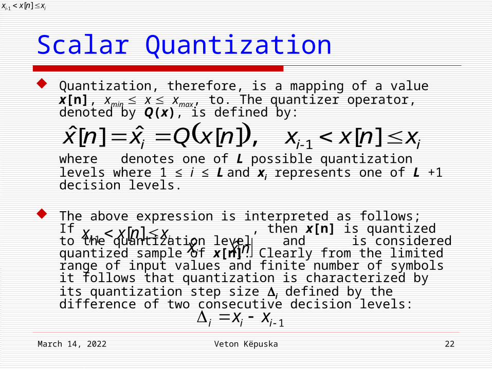
Scalar Quantization Quantization, therefore, is a mapping of a value x[n], xmin
x xmax, to. The quantizer operator, denoted by Q(x), is defined by:
where denotes one of L possible quantization levels where 1 ≤ i ≤ L and xi represents one of L +1 decision levels.
The above expression is interpreted as follows; If , then x[n] is quantized to the quantization level and is considered quantized sample of x[n]. Clearly from the limited range of input values and finite number of symbols it follows that quantization is characterized by its quantization step size i defined by the difference of two consecutive decision levels:
ii-i xnxxnxQxnx ][ ,][ˆ][ˆ 1
ii- xnxx ][1
ii- xnxx ][1
ix̂ nx̂
1 iii xx
April 19, 2023 Veton Këpuska 23
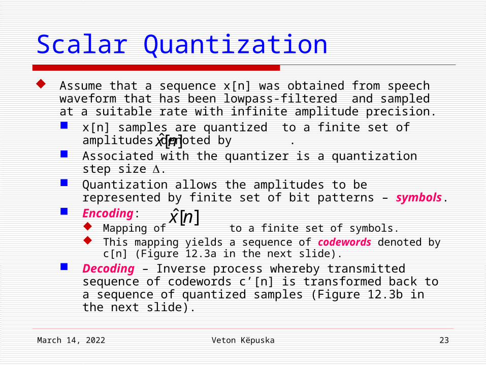
Scalar Quantization Assume that a sequence x[n] was obtained from speech
waveform that has been lowpass-filtered and sampled at a suitable rate with infinite amplitude precision. x[n] samples are quantized to a finite set of amplitudes
denoted by . Associated with the quantizer is a quantization step size. Quantization allows the amplitudes to be represented by
finite set of bit patterns – symbols. Encoding:
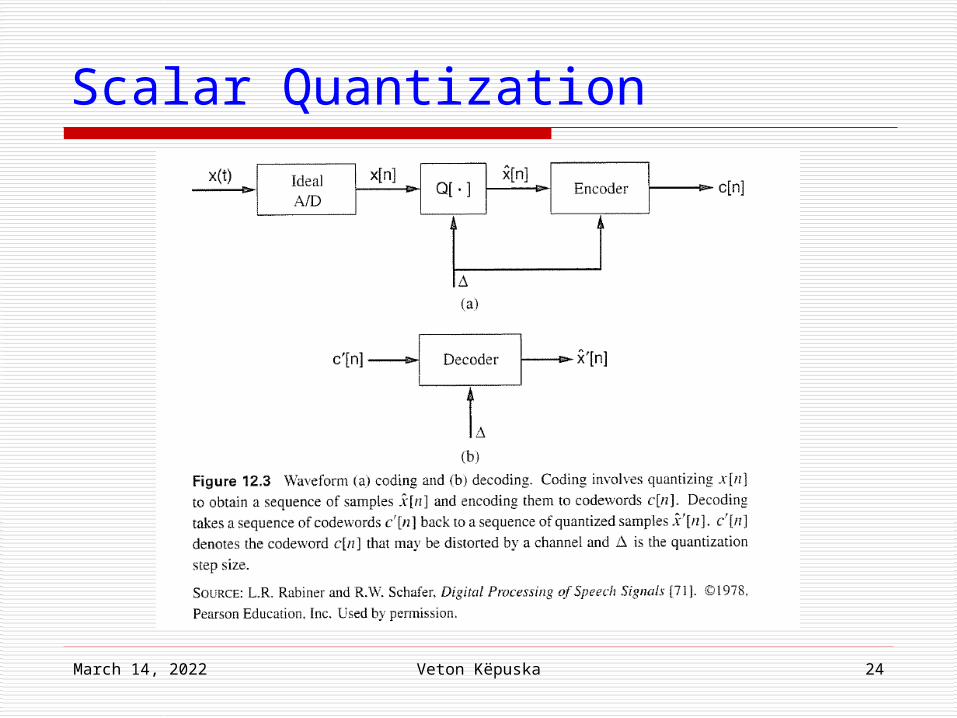
Mapping of to a finite set of symbols. This mapping yields a sequence of codewords denoted by c[n]
(Figure 12.3a in the next slide). Decoding – Inverse process whereby transmitted sequence
of codewords c’[n] is transformed back to a sequence of quantized samples (Figure 12.3b in the next slide).
][ˆ nx
][ˆ nx
April 19, 2023 Veton Këpuska 24
Scalar Quantization
April 19, 2023 Veton Këpuska 25
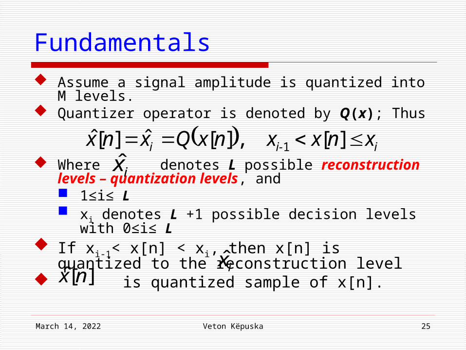
Fundamentals Assume a signal amplitude is quantized into M
levels. Quantizer operator is denoted by Q(x); Thus
Where denotes L possible reconstruction levels – quantization levels, and 1≤i≤ L xi denotes L +1 possible decision levels with
0≤i≤ L If xi-1< x[n] < xi, then x[n] is quantized to the
reconstruction level is quantized sample of x[n].
ii-i xnxxnxQxnx ][ ,][ˆ][ˆ 1
ix̂
ix̂
][ˆ nx
April 19, 2023 Veton Këpuska 26
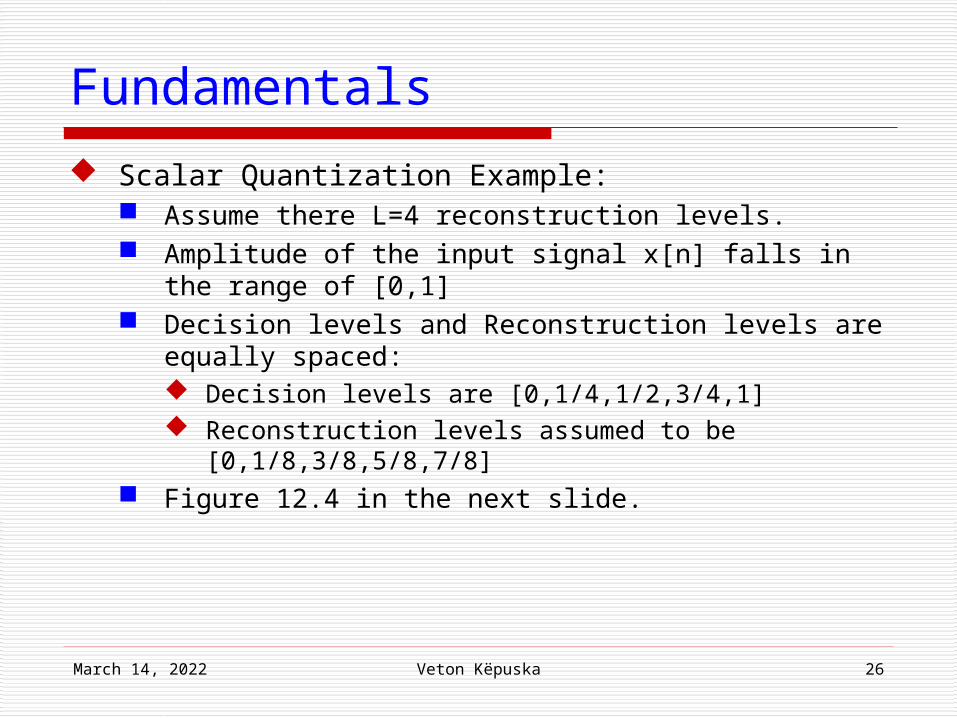
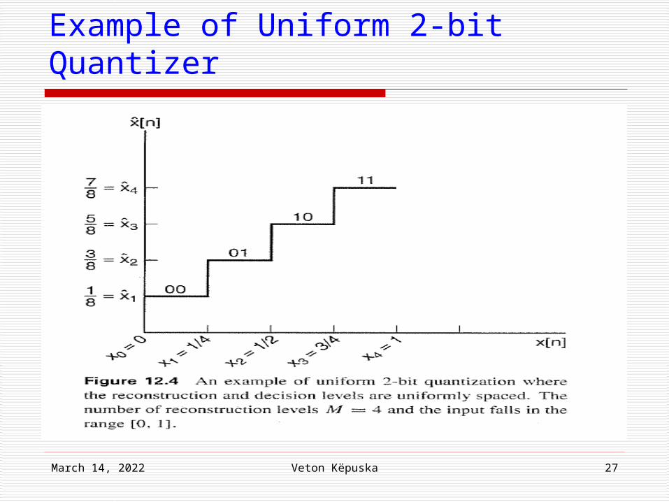
Fundamentals
Scalar Quantization Example: Assume there L=4 reconstruction levels. Amplitude of the input signal x[n] falls in the range of
[0,1] Decision levels and Reconstruction levels are equally
spaced: Decision levels are [0,1/4,1/2,3/4,1] Reconstruction levels assumed to be
[0,1/8,3/8,5/8,7/8] Figure 12.4 in the next slide.
April 19, 2023 Veton Këpuska 27
Example of Uniform 2-bit Quantizer
April 19, 2023 Veton Këpuska 28
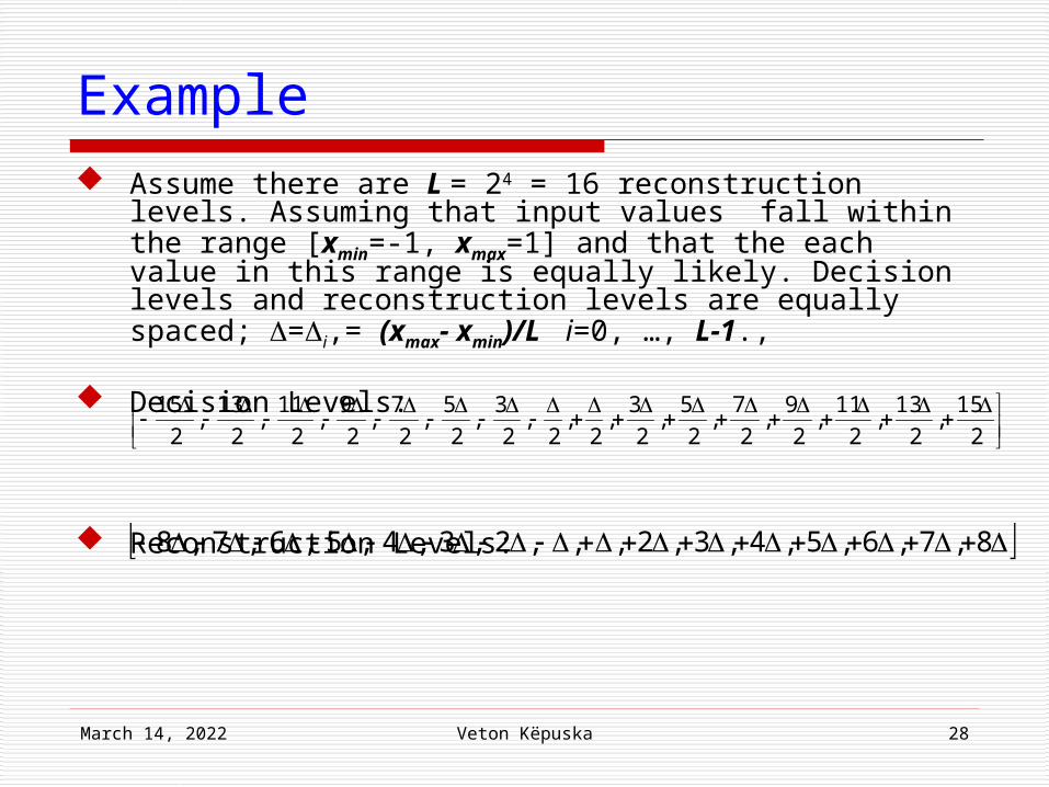
Example Assume there are L = 24 = 16 reconstruction levels.
Assuming that input values fall within the range [xmin=-1, xmax=1] and that the each value in this range is equally likely. Decision levels and reconstruction levels are equally spaced; =i,= (xmax- xmin)/L i=0, …, L-1.,
Decision Levels:
Reconstruction Levels:
2
15,
2
13,
2
11,
2
9,
2
7,
2
5,
2
3,
2,
2,
2
3,
2
5,
2
7,
2
9,
2
11,
2
13,
2
15
8,7,6,5,4,3,2,,,2,3,4,5,6,7,8
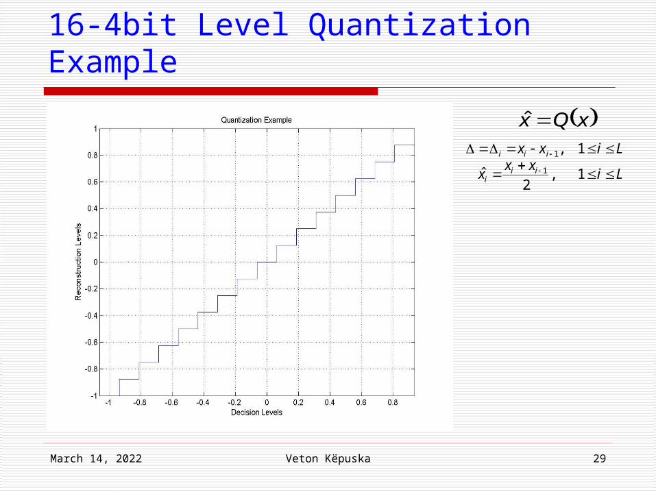
April 19, 2023 Veton Këpuska 29
16-4bit Level Quantization Example
xQx ˆ
1,
2ˆ
1 ,
1
1
Lixx
x
Lixx
iii
iii
April 19, 2023 Veton Këpuska 30
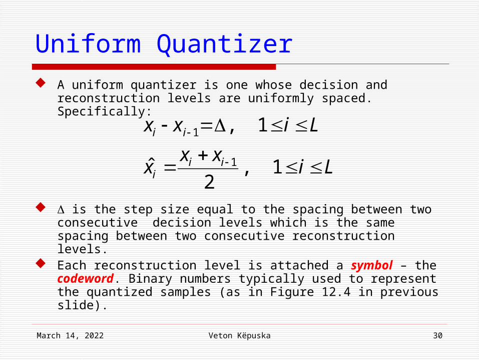
Uniform Quantizer A uniform quantizer is one whose decision and
reconstruction levels are uniformly spaced. Specifically:
is the step size equal to the spacing between two consecutive decision levels which is the same spacing between two consecutive reconstruction levels.
Each reconstruction level is attached a symbol – the codeword. Binary numbers typically used to represent the quantized samples (as in Figure 12.4 in previous slide).
Lixx
x
Lixx
iii
ii
1 ,2
ˆ
1 ,
1
1
April 19, 2023 Veton Këpuska 31
Uniform Quantizer Codebook: Collection of codewords. In general with B-bit binary codebook there are 2B different
quantization (or reconstruction) levels. Bit rate is defined as the number of bits B per sample
multiplied by sample rate fs:
I=Bfs
Decoder inverts the coder operation taking the codeword back to a quantized amplitude value (e.g., 01 → ).
Often the goal of speech coding/decoding is to maintain the bit rate as low as possible while maintaining a required level of quality.
Because sampling rate is fixed for most applications this goal implies that the bit rate be reduced by decreasing the number of bits per sample
2x̂
April 19, 2023 Veton Këpuska 32
Uniform Quantizer Designing a uniform scalar quantizer requires
knowledge of the maximum value of the sequence. Typically the range of the speech signal is
expressed in terms of the standard deviation of the signal. Specifically, it is often assumed that: -4x≤x[n]≤4x
where x is signal’s standard deviation. Under the assumption that speech samples obey
Laplacian pdf there are approximately 0.35% of speech samples fall outside of the range: -4x≤x[n]≤4x.
Assume B-bit binary codebook ⇒ 2B. Maximum signal value xmax = 4x.
April 19, 2023 Veton Këpuska 33
Uniform Quantizer
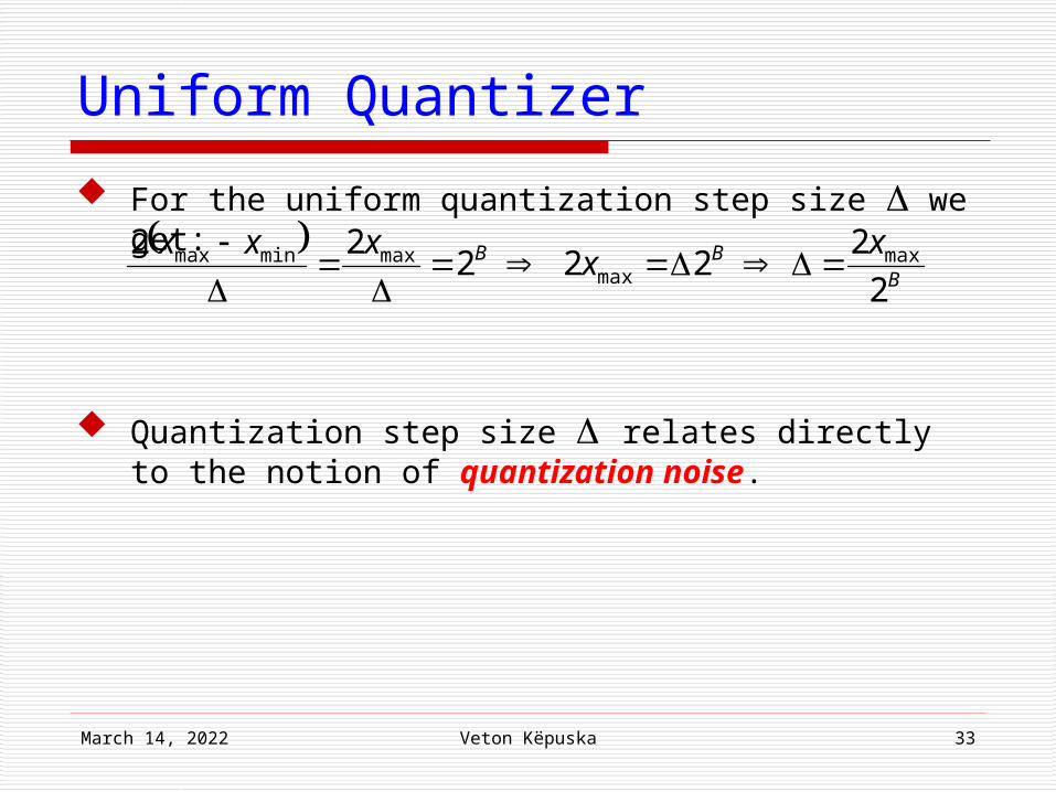
For the uniform quantization step size we get:
Quantization step size relates directly to the notion of quantization noise.
B
BB xx
xxx
2
2 22 2
22 maxmax
maxminmax
April 19, 2023 Veton Këpuska 34
Quantization Noise
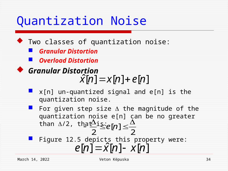
Two classes of quantization noise: Granular Distortion Overload Distortion
Granular Distortion
x[n] un-quantized signal and e[n] is the quantization noise.
For given step size the magnitude of the quantization noise e[n] can be no greater than /2, that is:
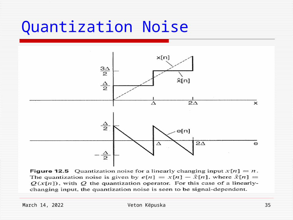
Figure 12.5 depicts this property were:
][][][ˆ nenxnx
2][
2
ne
][][ˆ][ nxnxne
April 19, 2023 Veton Këpuska 35
Quantization Noise
April 19, 2023 Veton Këpuska 36
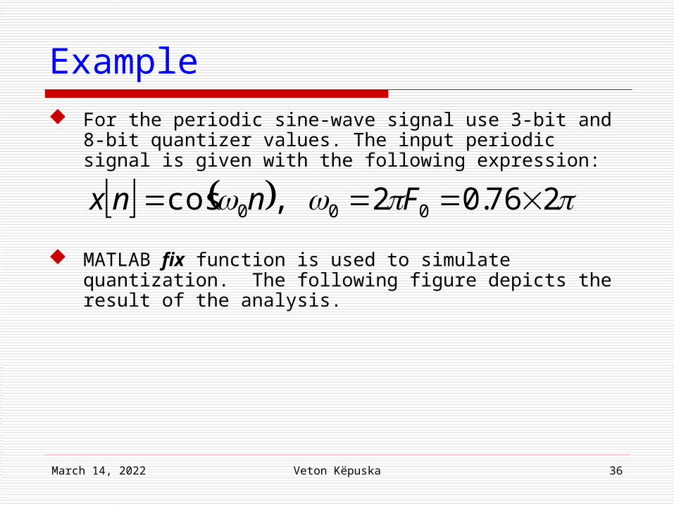
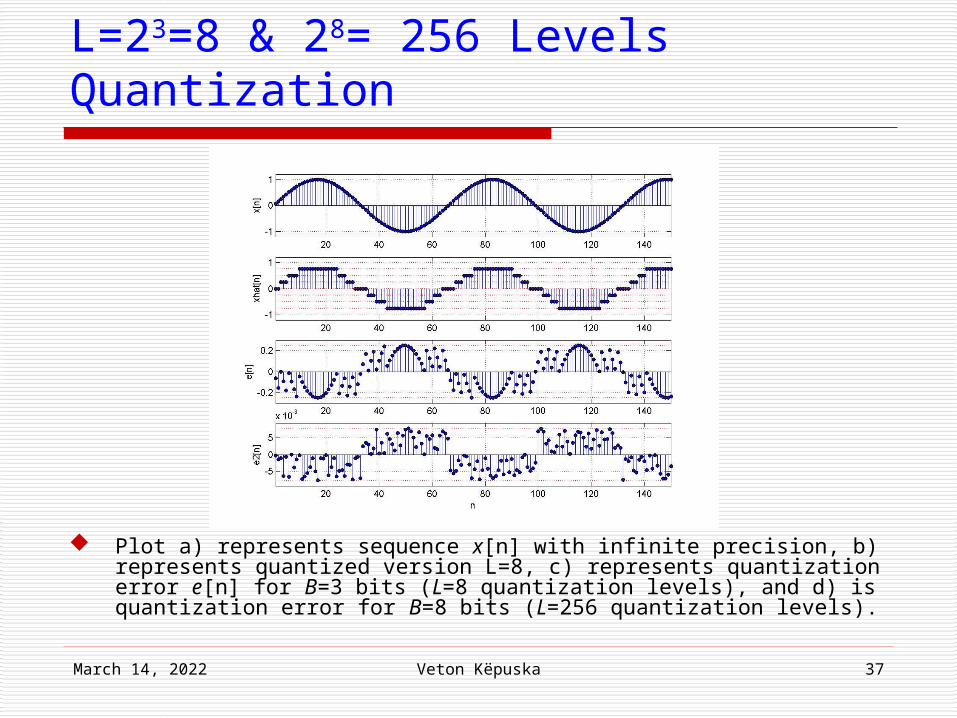
Example For the periodic sine-wave signal use 3-bit and 8-bit
quantizer values. The input periodic signal is given with the following expression:
MATLAB fix function is used to simulate quantization. The following figure depicts the result of the analysis.
276.02,cos 000 Fnnx
April 19, 2023 Veton Këpuska 37
L=23=8 & 28= 256 Levels Quantization
Plot a) represents sequence x[n] with infinite precision, b) represents quantized version L=8, c) represents quantization error e[n] for B=3 bits (L=8 quantization levels), and d) is quantization error for B=8 bits (L=256 quantization levels).
April 19, 2023 Veton Këpuska 38
Quantization Noise
Overload Distortion Maximum-value constant: xmax = 4x (4x≤x[n]≤4x) For Laplacian pdf, 0.35% of the speech
samples fall outside the range of the quantizer.
Clipped samples incur a quantization error in excess of /2.
Due to the small number of clipped samples it is common to neglect the infrequent large errors in theoretical calculations.
April 19, 2023 Veton Këpuska 39
Quantization Noise
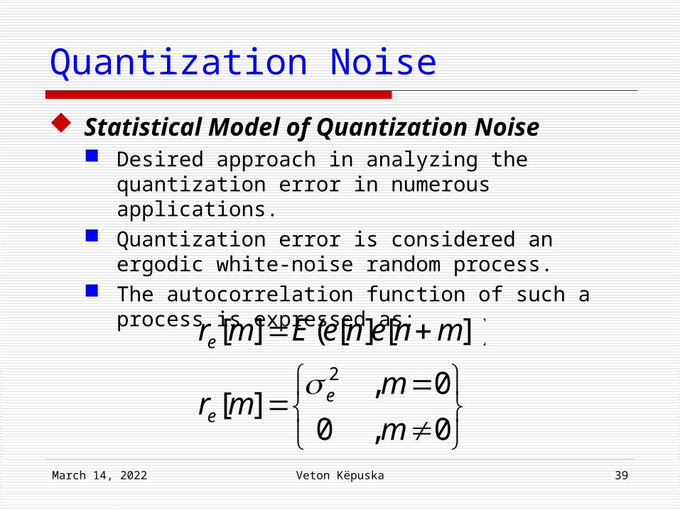
Statistical Model of Quantization Noise Desired approach in analyzing the quantization
error in numerous applications. Quantization error is considered an ergodic
white-noise random process. The autocorrelation function of such a process is
expressed as:
0,0
0,][
])[][(][2
m
mmr
mneneEmr
ee
e
April 19, 2023 Veton Këpuska 40
Quantization Error
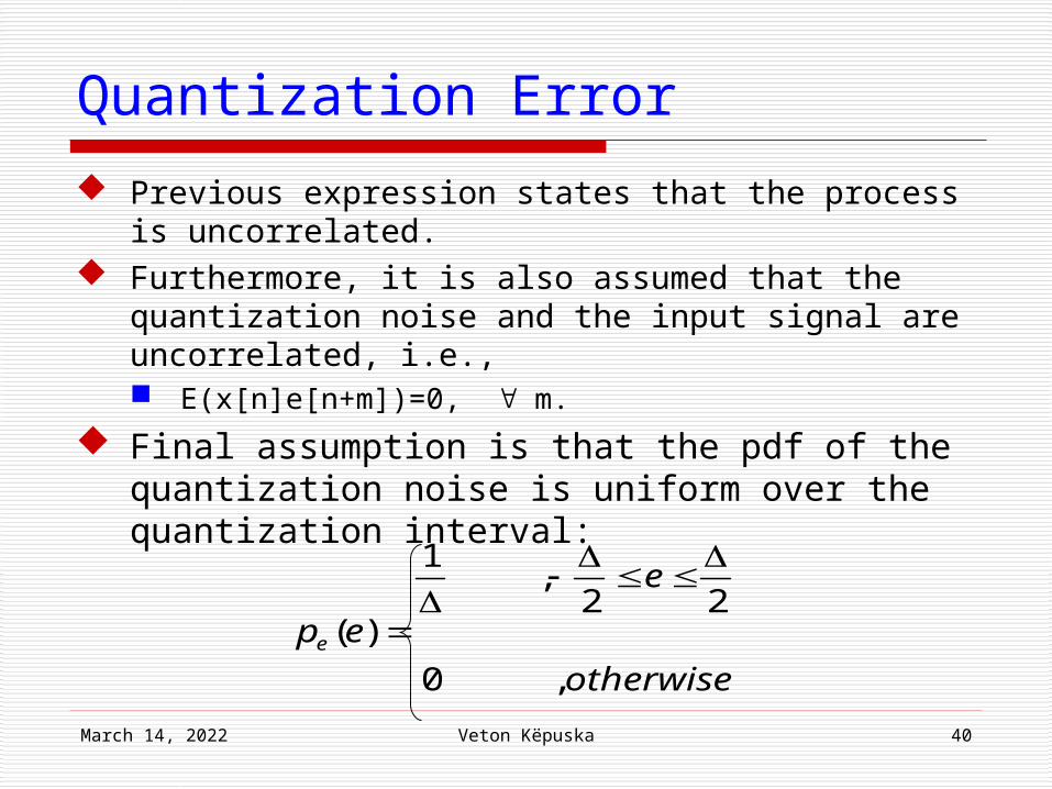
Previous expression states that the process is uncorrelated.
Furthermore, it is also assumed that the quantization noise and the input signal are uncorrelated, i.e., E(x[n]e[n+m])=0, m.
Final assumption is that the pdf of the quantization noise is uniform over the quantization interval:
otherwise
e
epe
,0
22,
1
)(
April 19, 2023 Veton Këpuska 41
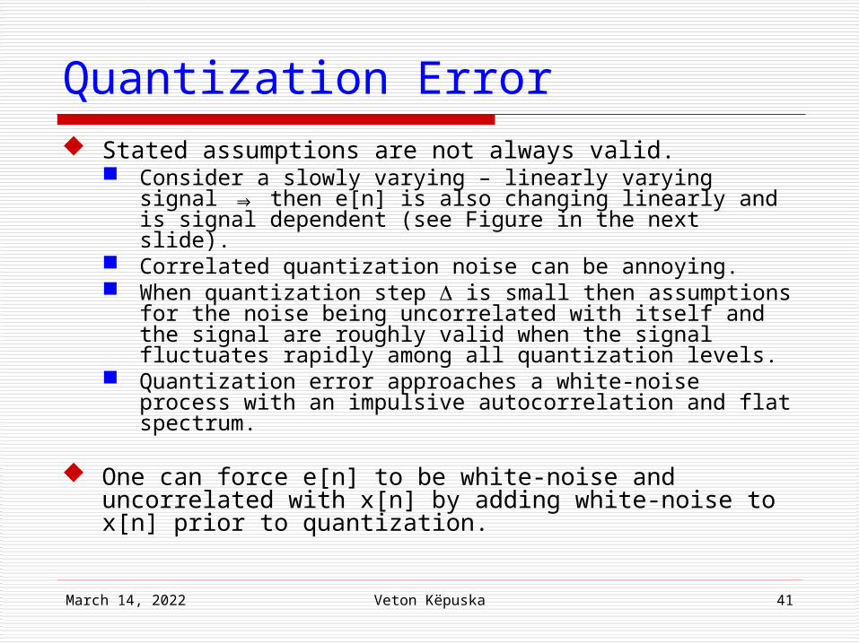
Quantization Error Stated assumptions are not always valid.
Consider a slowly varying – linearly varying signal ⇒ then e[n] is also changing linearly and is signal dependent (see Figure in the next slide).
Correlated quantization noise can be annoying. When quantization step is small then assumptions
for the noise being uncorrelated with itself and the signal are roughly valid when the signal fluctuates rapidly among all quantization levels.
Quantization error approaches a white-noise process with an impulsive autocorrelation and flat spectrum.
One can force e[n] to be white-noise and uncorrelated with x[n] by adding white-noise to x[n] prior to quantization.
April 19, 2023 Veton Këpuska 42
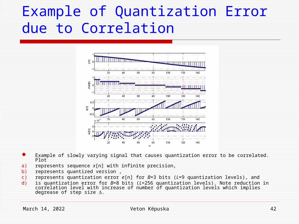
Example of Quantization Error due to Correlation
Example of slowly varying signal that causes quantization error to be correlated. Plot a) represents sequence x[n] with infinite precision, b) represents quantized version , c) represents quantization error e[n] for B=3 bits (L=9 quantization levels), and d) is quantization error for B=8 bits (L=256 quantization levels). Note reduction in
correlation level with increase of number of quantization levels which implies degrease of step size .
April 19, 2023 Veton Këpuska 43
Quantization Error
Process of adding white noise is known as Dithering.
This decorrelation technique was shown to be useful not only in improving the perceptual quality of the quantization noise but also with image signals.
Signal-to-Noise Ratio A measure to quantify severity of the
quantization noise. Relates the strength of the signal to the strength
of the quantization noise.
April 19, 2023 Veton Këpuska 44
Quantization Error
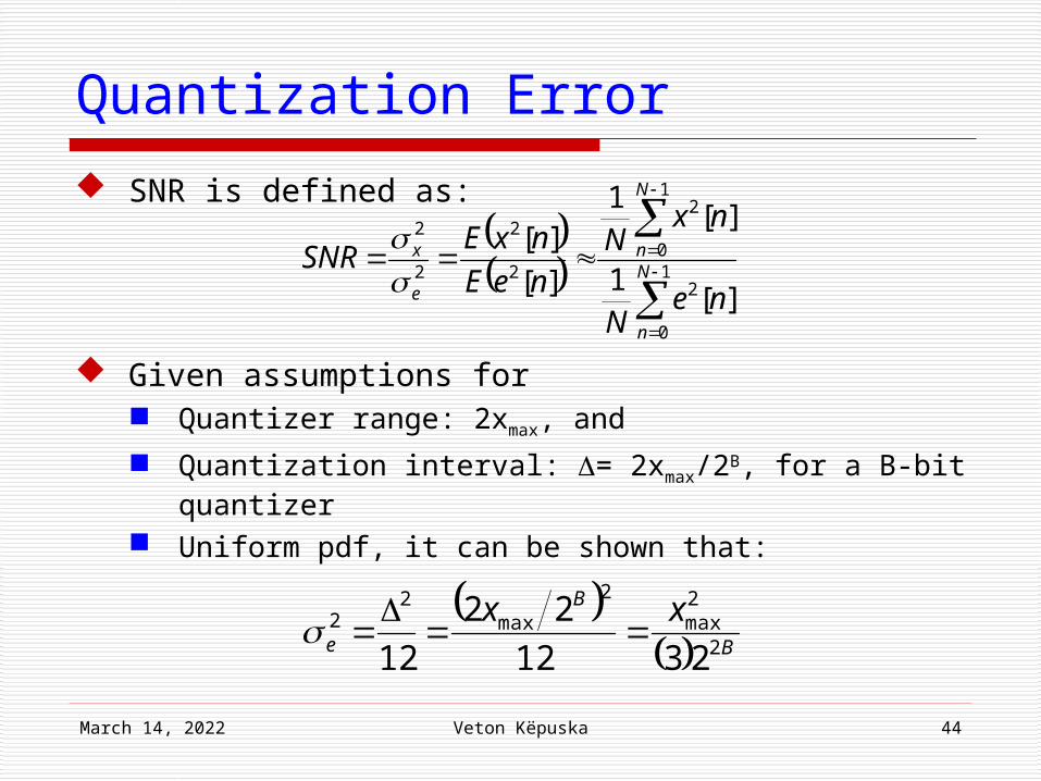
SNR is defined as:
Given assumptions for Quantizer range: 2xmax, and
Quantization interval: = 2xmax/2B, for a B-bit quantizer
Uniform pdf, it can be shown that:
1
0
2
1
0
2
2
2
2
2
][1
][1
][
][N
n
N
n
e
x
neN
nxN
neE
nxESNR
B
B
e
xx2
2max
2
max2
2
2312
22
12
April 19, 2023 Veton Këpuska 45
Quantization Error
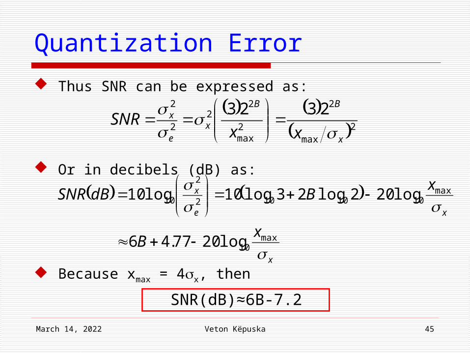
Thus SNR can be expressed as:
Or in decibels (dB) as:
Because xmax = 4x, then
2max
2
2max
22
2
2 2323
x
BB
xe
x
xxSNR
x
xe
x
xB
xBdBSNR
max10
max1010102
2
10
log2077.46
log202log23log10log10
SNR(dB)≈6B-7.2
April 19, 2023 Veton Këpuska 46
Quantization Error Presented quantization scheme is called pulse code
modulation (PCM). B-bits per sample are transmitted as a codeword. Advantages of this scheme:
It is instantaneous (no coding delay) Independent of the signal content (voice, music, etc.)
Disadvantages: It requires minimum of 11 bits per sample to achieve “toll
quality” (equivalent to a typical telephone quality) For 10,000 Hz sampling rate, the required bit rate is:
B=(11 bits/sample)x(10000 samples/sec)=110,000 bps=110 kbps
For CD quality signal with sample rate of 20,000 Hz and 16-bits/sample, SNR(dB) =96-7.2=88.8 dB and bit rate of 320 kbps.
April 19, 2023 Veton Këpuska 47
Nonuniform Quantization Uniform quantization may not be optimal (SNR can not
be as small as possible for certain number of decision and reconstruction levels)
Consider for example speech signal for which x[n] is much more likely to be in one particular region than in other (low values occurring much more often than the high values).
This implies that decision and reconstruction levels are not being utilized effectively with uniform intervals over xmax.
A Nonuniform quantization that is optimal (in a least-squared error sense) for a particular pdf is referred to as the Max quantizer.
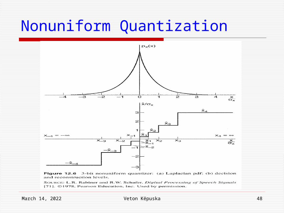
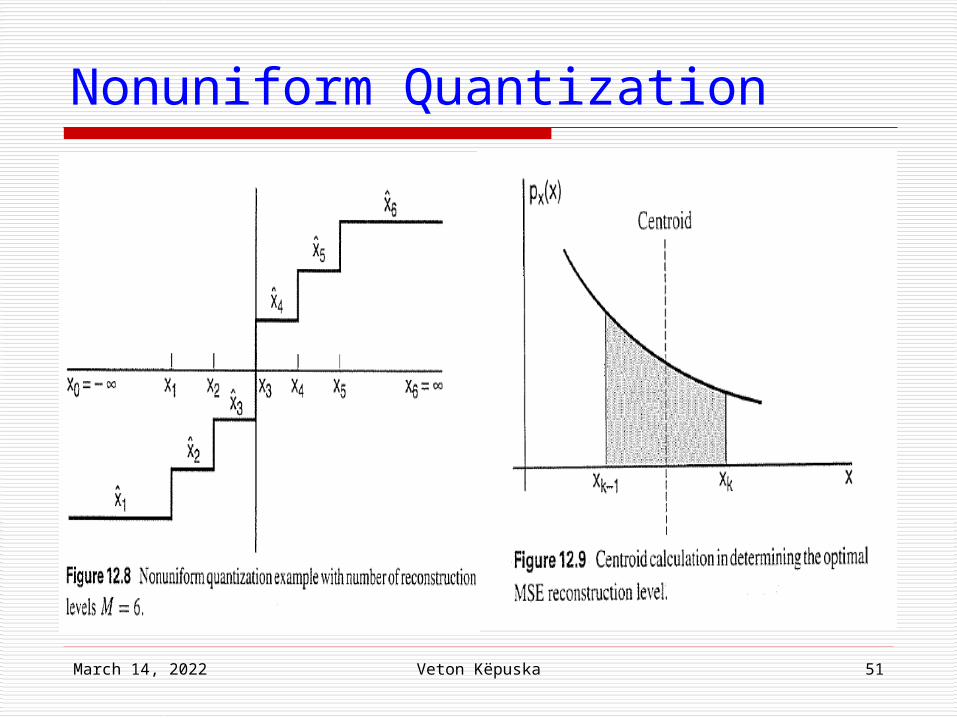
Example of a nonuniform quantizer is given in the figure in the next slide.
April 19, 2023 Veton Këpuska 48
Nonuniform Quantization
April 19, 2023 Veton Këpuska 49
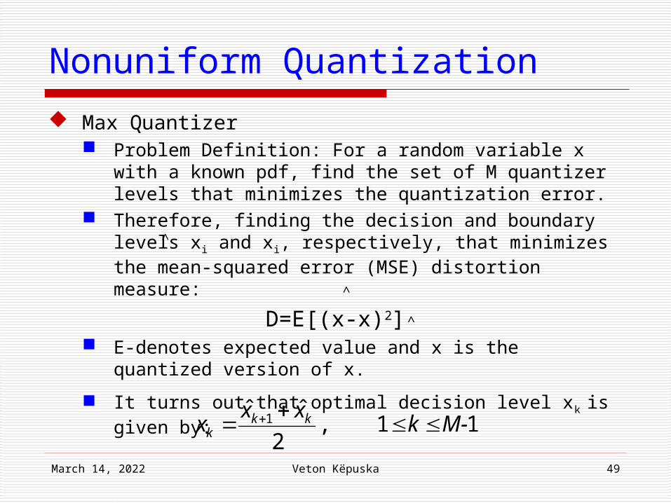
Nonuniform Quantization
Max Quantizer Problem Definition: For a random variable x with a
known pdf, find the set of M quantizer levels that minimizes the quantization error.
Therefore, finding the decision and boundary levels xi and xi, respectively, that minimizes the mean-squared error (MSE) distortion measure:
D=E[(x-x)2] E-denotes expected value and x is the quantized
version of x.
It turns out that optimal decision level xk is given by:
^
^
^
11 ,2
ˆˆ 1 M-kxx
x kkk
April 19, 2023 Veton Këpuska 50
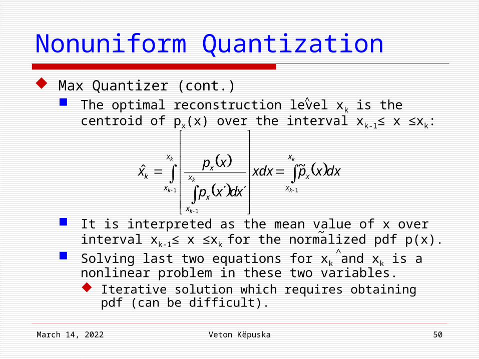
Nonuniform Quantization Max Quantizer (cont.)
The optimal reconstruction level xk is the centroid of px(x) over the interval xk-1≤ x ≤xk:
It is interpreted as the mean value of x over interval xk-1≤ x ≤xk for the normalized pdf p(x).
Solving last two equations for xk and xk is a nonlinear problem in these two variables. Iterative solution which requires obtaining pdf (can
be difficult).
^
k
k
k
k
k
k
x
x
x
x
xx
x
x
xk dxxpxdx
xdxp
xpx
11
1
~ˆ
~
^
April 19, 2023 Veton Këpuska 51
Nonuniform Quantization
Companding
A fixed non-uniform quantizer
April 19, 2023 Veton Këpuska 53
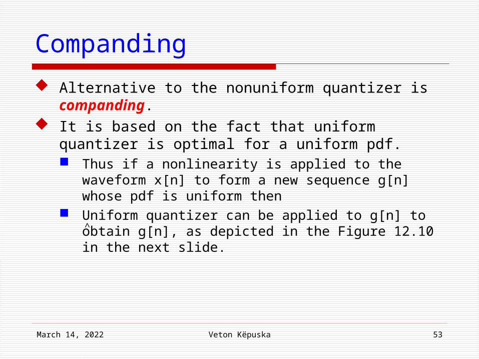
Companding
Alternative to the nonuniform quantizer is companding.
It is based on the fact that uniform quantizer is optimal for a uniform pdf. Thus if a nonlinearity is applied to the waveform x[n]
to form a new sequence g[n] whose pdf is uniform then
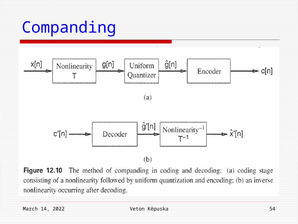
Uniform quantizer can be applied to g[n] to obtain g[n], as depicted in the Figure 12.10 in the next slide. ^
April 19, 2023 Veton Këpuska 54
Companding
April 19, 2023 Veton Këpuska 55
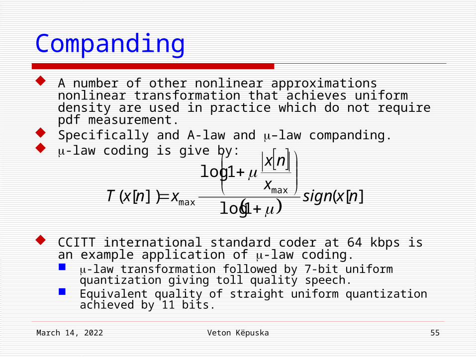
Companding A number of other nonlinear approximations nonlinear
transformation that achieves uniform density are used in practice which do not require pdf measurement.
Specifically and A-law and –law companding. -law coding is give by:
CCITT international standard coder at 64 kbps is an example application of -law coding. -law transformation followed by 7-bit uniform quantization
giving toll quality speech. Equivalent quality of straight uniform quantization achieved
by 11 bits.
])[(1log
1log
])[( maxmax nxsign
x
nx
xnxT
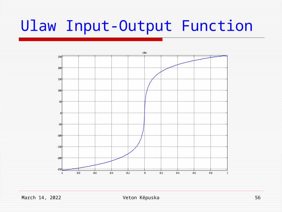
Ulaw Input-Output Function
April 19, 2023 Veton Këpuska 56
-1 -0.8 -0.6 -0.4 -0.2 0 0.2 0.4 0.6 0.8 1-250
-200
-150
-100
-50
0
50
100
150
200
250
ulaw

Adaptive Coding

April 19, 2023 Veton Këpuska 58
Adaptive Coding Nonuniform quantizers are optimal for a long term pdf of
speech signal. However, considering that speech is a highly-time-
varying signal, one has to question if a single pdf derived from a long-time speech waveform is a reasonable assumption.
Changes in the speech waveform: Temporal and spectral variations due to transitions from
unvoiced to voiced speech, Rapid volume changes.
Approach: Estimate a short-time pdf derived over 20-40 msec
intervals. Short-time pdf estimates are more accurately described by
a Gaussian pdf regardless of the speech class.

April 19, 2023 Veton Këpuska 59
Adaptive Coding
A pdf (e.g., Gaussian) derived from a short-time speech segment more accurately represents the speech nonstationarity.
One approach is to assume a pdf of a specific shape in particular a Gaussian with unknown variance 2. Measure the local variance then adapt a nonuniform
quantizer to the resulting local pdf. This approach is referred to as adaptive
quantization.
For a Gaussian we have:2
2
2
22
1)( x
x
x
x exp

April 19, 2023 Veton Këpuska 60
Adaptive Coding
Measure the variance x2 of a sequence x[n] and
use resulting pdf to design optimal max quantizer. Note that a change in the variance simply scales
the time signal: If E(x2[n]) = x
2 then E[(x [n])2] = 2 x2
1. Need to design only one nonuniform quantizer with unity variance and scale decision and reconstruction levels according to a particular variance.
2. Fix the quantizer and apply a time-varying gain to the signal according to the estimated variance (scale the signal to match the quantizer).

April 19, 2023 Veton Këpuska 61
Adaptive Coding

April 19, 2023 Veton Këpuska 62
Adaptive Coding There are two possible approaches for estimation of a
time-varying variance 2[n]: Feed-forward method (shown in Figure 12.11) where the
variance (or gain) estimate is obtained from the input Feedback method where the estimate is obtained from a
quantizer output. Advantage – no need to transmit extra side information
(quantized variance) Disadvantage – additional sensitivity to transmission errors
in codewords. Adaptive quantizers can achieve higher SNR than the
use of –law companding. –law companding is generally preferred for high-rate
waveform coding because of its lower background noise when transmission channel is idle. Why?
Adaptive quantization is useful in variety of other coding schemes.

Differential and Residual Quantization

April 19, 2023 Veton Këpuska 64
Differential and Residual Quantization
Presented methods are examples of instantaneous quantization.
Those approaches do not take advantage of the fact that speech is highly correlated signal: Short-time (10-15 samples), as well as Long-time (over a pitch period)
In this section methods that exploit short-time correlation will be investigated.

April 19, 2023 Veton Këpuska 65
Differential and Residual Quantization
Short-time Correlation: Neighboring samples are “self-similar”, that is, not changing too
rapidly from one another. Difference of adjacent samples should have a lower variance than
the variance of the signal itself. This difference, thus, would make a more effective use of
quantization levels: Higher SNR for fixed number of quantization levels. Predicting the next sample from previous ones (finding the best
prediction coefficients to yield a minimum mean-squared prediction error same methodology as in Liner Prediction Coefficients - LPC). Two approaches:1. Have a fixed prediction filter to reflect the average local
correlation of the signal.2. Allow predictor to short-time adapt to the signal’s local
correlation. Requires transmission of quantized prediction
coefficients as well as the prediction error.

April 19, 2023 Veton Këpuska 66
Differential and Residual Quantization
Illustration of a particular error encoding scheme presented in the Figure 12.12 of the next slide.
In this scheme the following sequences are required: x[n] – prediction of the input sample x[n]; This is the
output of the predictor P(z) whose input is a quantized version of the input signal x[n], i.e., x[n]
r[n] – prediction error signal; residual r[n] – quantized prediction error signal.
This approach is sometimes referred to as residual coding.
~
^
^

April 19, 2023 Veton Këpuska 67
Differential and Residual Quantization

April 19, 2023 Veton Këpuska 68
Differential and Residual Quantization
Quantizer in the previous scheme can be of any type: Fixed Adaptive Uniform Nonuniform
Whatever the case is, the parameter of the quantizer are determined so that to match variance of r[n].
Differential quantization can also be applied to: Speech signal Parameters that represent speech:
LPC – linear prediction coefficients Cepstral coefficients obtained from Homomorphic filtering. Sinewave parameters, etc.

April 19, 2023 Veton Këpuska 69
Differential and Residual Quantization
Consider quantization error of the quantized residual:
From Figure 12.12 we express the quantized input x[n] as:
][][][ˆ nenrnr r
^
][][
][][~][][~][][][~
][ˆ][~][ˆ
nenx
nenxnxnx
nenrnx
nrnxnx
r
r
r
Q
+
][ˆ nr+
][nr
P(z)][ˆ nx][~ nx
][nx+
-

April 19, 2023 Veton Këpuska 70
Differential and Residual Quantization
Quantized signal samples differ form the input only by the quantization error er[n].
Since the er[n] is the quantization error of the residual: ⇒ if the prediction of the signal is accurate then the
variance of r[n] will be smaller than the variance of x[n]
⇒ A quantizer with a given number of levels can be adjusted to give a smaller quantization error than would be possible when quantizing the signal directly.

April 19, 2023 Veton Këpuska 71
Differential and Residual Quantization The differential coder of Figure 12.12 is referred to:
Differential PCM (DPCM) when used with a fixed predictor and fixed quantization.
Adaptive Differential PCM (ADPCM) when used with Adaptive prediction (i.e., adapting the predictor to local
correlation) Adaptive quantization (i.e., adapting the quantizer to the local
variance of r[n]) ADPCM yields greatest gains in SNR for a fixed bit rate.
The international coding standard CCITT, G.721 with toll quality speech at 32 kbps (8000 samples/sec x 4 bits/sample) has been designed based on ADPCM techniques.
To achieve higher quality with lower rates it is required to: Rely on speech model-based techniques and The exploiting of long-time prediction, as well as Short-time prediction

April 19, 2023 Veton Këpuska 72
Differential and Residual Quantization
Important variation of the differential quantization scheme of Figure 12.12. Prediction has assumed an all-pole model
(autoregressive model). In this model signal value is predicted from its past
samples: Any error in a codeword due to for example bit errors
over a degraded channel propagate over considerable time during decoding.
Such error propagation is severe when the signal values represent speech model parameters computed frame-by frame (as opposed to sample-by-sample).
Alternative approach is to use a finite-order moving-average predictor derived from the residual.
One common approach of the use of the moving-average predictor is illustrated in Figure 12.13 in the next slide.

April 19, 2023 Veton Këpuska 73
Differential and Residual Quantization

April 19, 2023 Veton Këpuska 74
Differential and Residual Quantization
Coder Stage of the system in Figure 12.13: Residual as the difference of the true value and the value
predicted from the moving average of K quantized residuals:
p[k] – coefficients of P(z) Decoder Stage:
Predicted value is given by:
Error propagation is thus limited to only K samples (or K analysis frames for the case of model parameters)
K
k
knrkpnanr1
][ˆ][][][
K
k
knrkpnrna1
][ˆ][][ˆ][ˆ

Vector Quantization

April 19, 2023 Veton Këpuska 76
Vector Quantization (VQ)
Investigation of scalar quantization techniques was the topic of previous sections.
A generalization of scalar quantization referred to as vector quantization is investigated in this section.
In vector quantization a block of scalars are coded as a vector rather than individually.
An optimal quantization strategy can be derived based on a mean-squared error distortion metric as with scalar quantization.

April 19, 2023 Veton Këpuska 77
Vector Quantization (VQ) Motivation
Assume the vocal tract transfer function is characterized by only two resonance's thus requiring four reflection coefficients.
Furthermore, suppose that the vocal tract can take on only one of possible four shapes.
This implies that there exist only four possible sets of the four reflection coefficients as illustrated in Figure 12.14 in the next slide.
Scalar Quantization – considers each of the reflection coefficient individually: Each coefficient can take on 4 different values
⇒ 2 bits required to encode each coefficient. For 4 reflection coefficients it is required 4x2=8 bits per analysis frame
to code the vocal tract transfer function. Vector Quantization – since there are only four possible vocal tract
positions of the vocal tract corresponding to only four possible vectors of reflection coefficients. Scalar values of each vector are highly correlated. Thus 2 bits are required to encode the 4 reflection coefficients.
Note: if scalars were independent of each other treating them together as a vector would have no advantage over treating them individually.

April 19, 2023 Veton Këpuska 78
Vector Quantization (VQ)

April 19, 2023 Veton Këpuska 79
Vector Quantization (VQ)
Consider a vector of N continuous scalars:
With VQ, the vector x is mapped into another N-dimensional vector x:
Vector x is chosen from M possible reconstruction (quantization) levels:
^
TNxxxxx ˆ,...,ˆ,ˆ,ˆˆ 321
TNxxxxx ,...,,, 321
^
ii CxrxVQx for ,][ˆ

April 19, 2023 Veton Këpuska 80
Vector Quantization (VQ)
T
T

April 19, 2023 Veton Këpuska 81
Vector Quantization (VQ)
VQ-vector quantization operator ri-M possible reconstruction levels for
1≤i<M Ci-ith “cell” or cell boundary
If x is in the cell Ci, then x is mapped to ri. ri – codeword
{ri} – set of all codewords; codebook.

April 19, 2023 Veton Këpuska 82
Vector Quantization (VQ)
Properties of VQ:P1: In vector quantization a cell can
have an arbitrary size and shape.In scalar quantization a “cell” (region between two decision levels) can have an arbitrary size, but it’s shape is fixed.
P2: Similarly to scalar quantization, distortion measure D(x,x), is a measure of dissimilarity or error between x and x.
^
^

April 19, 2023 Veton Këpuska 83
VQ Distortion Measure
Vector quantization noise is represented by the vector e:
The distortion is the average of the sum of squares of scalar components:
For the multi-dimensional pdf px(x):
xxe ˆ
eeED T
xdxpxrxr
xdxpxxxxxxxxED
xiT
i
M
iCx
xTT
i
1
...
ˆˆ...ˆˆ

April 19, 2023 Veton Këpuska 84
VQ Distortion Measure Goal to minimize:
Two conditions formulated by Lim:C1: A vector x must be quantized to a reconstruction level ri
that gives the smallest distortion between x and ri. C2: Each reconstruction level ri must be the centroid of the
corresponding decision region (cell Ci)
Condition C1 implies that given the reconstruction levels we can quantize without explicit need for the cell boundaries. To quantize a given vector the reconstruction level is found
which minimizes its distortion. This process requires a large search – active area of research.
Condition C2 specifies how to obtain a reconstruction level from the selected cell.
xxxxED T ˆˆ

April 19, 2023 Veton Këpuska 85
VQ Distortion Measure
Stated 2 conditions provide the basis for iterative solution of how to obtain VQ codebook. Start with initial estimate of ri.
Apply condition 1 by which all the vectors from a set that get quantized by ri can be determined.
Apply second condition to obtain a new estimate of the reconstruction levels (i.e., centroid of each cell)
Problem with this approach is that it requires estimation of joint pdf of all x in order to compute the distortion measure and the multi-dimensional centroid.
Solution: k-means algorithm (Lloyd for 1-D and Forgy for multi-D).

April 19, 2023 Veton Këpuska 86
k-Means Algorithm1. Compute the ensemble average D as:
xk are the training vectors and xk are the quantized vectors.
2. Pick an initial guess at the reconstruction levels {ri}3. For each xk select closest ri. Set of all xk nearest to ri
forms a cluster (see Figure 12.16) – “clustering algorithm”.
4. Compute the mean of xk in each cluster which gives a new ri’s. Calculate D.
5. Stop when the change in D over two consecutive interactions is insignificant.
This algorithm converges to a local minimum of D.
)ˆ()ˆ(1 1
0kk
Tk
N
kk xxxx
ND
^

April 19, 2023 Veton Këpuska 87
k-Means Algorithm

April 19, 2023 Veton Këpuska 88
Neural Networks Based Clustering Algorithms
Kohonen’s SOFM Topological Ordering of the SOFM Offers potential for further reduction in bit rate.

April 19, 2023 Veton Këpuska 89
Use of VQ in Speech Transmission
Obtain the VQ codebook from the training vectors - all transmitters and receivers must have identical copies of VQ codebook.
Analysis procedure generates a vector xi. Transmitter sends the index of the centroid
ri of the closest cluster for the given vector xi. This step involves search.
Receiving end decodes the information by accessing the codeword of the received index and performing synthesis operation.

Model-Based Coding
Liner Prediction Method (LPC)

April 19, 2023 Veton Këpuska 91
Model-Based Coding The purpose of model-based speech coding is to
increase the bit efficiency to achieve either: Higher quality for the same bit rate or Lower bit rate for the same quality.
Chronological perspective of model-based coding starting with: All-pole speech representation used for coding:
Scalar Quantization Vector Quantization
Mixed Excitation Linear Prediction (MELP) coder: Remove deficiencies in binary source representation.
Code-excited Linear Prediction (CELP) coder: Does nor require explicit multi-band decision and source
characterization as MELP.

April 19, 2023 Veton Këpuska 92
Basic Linear Prediction Coder (LPC) Recall the basic speech production model of the form:
where the predictor polynomial is given as:
Suppose: Linear Prediction analysis performed at 100 frames/s 13 parameters are used:
10 all-pole spectrum parameters, Pitch Voicing decision Gain
Resulting in 1300 parameters/s. Compared to telephone quality signal:
4000 Hz bandwidth 8000 samples/s (8 bit per sample). 1300 parameters/s < 8000 samples/s
)(1)()(
zP
A
zA
AzH
p
k
kk zazP
1
)(

April 19, 2023 Veton Këpuska 93
Basic Linear Prediction Coder (LPC)
Instead of prediction coefficients ai use: Corresponding poles bi
Partial Correlation Coefficients ki (PARCOR) Reflection Coefficients ri, or Other equivalent representation.
Behavior of prediction coefficients is difficult to characterize: Large dynamic range ( large variance) Quantization errors can lead to unstable system function at
synthesis (poles may move outside the unit circle). Alternative equivalent representations:
Have a limited dynamic range Can be easily enforced to give stability because |bi|<1 and |
ki|<1.

April 19, 2023 Veton Këpuska 94
Basic Linear Prediction Coder (LPC)
Many ways to code linear prediction parameters: Ideally optimal quantization uses the Max quantizer based
on known or estimated pdf’s of each parameter. Example of 7200 bps coding:
1. Voice/Unvoiced Decision: 1 bit (on or off)2. Pitch (if voiced): 6 bits (uniform)3. Gain: 5 bits (nonuniform)4. Each Pole bi: 10 bits (nonuniform)
5 bits for bandwidth 5 bits for center frequency Total of 6 poles
100 frames/s 1+6+5+6x10=72 bits
Quality limited by simple impulse/noise excitation model.

April 19, 2023 Veton Këpuska 95
Basic Linear Prediction Coder (LPC)
Improvements possible based on replacement of poles with PARCOR. Higher order PARCOR have pdf’s closer to Gaussian centered
around zero nonuniform quantization. Companding is effective with PARCOR:
Transformed pdf’s close to uniform. Original PARCOR coefficients do not have a good spectral
sensitivity (change in spectrum with a change in spectral parameters that is desired to minimize).
Empirical finding that a more desirable transformation in this sense is to use logarithm of the vocal tract area function ratio:
i
i
i
iii
i
i
i
i
A
A
k
kkTg
k
k
A
A
1
1
log1
1log
1
1

April 19, 2023 Veton Këpuska 96
Basic Linear Prediction Coder (LPC)
Parameters gi: Have a pdf close to uniform Smaller spectral sensitivity than PARCOR:
The all pole spectrum changes less with a change in gi than with a change in ki
Note that spectrum changes less with the change in ki than with the change in pole positions.
Typically these parameters can be coded at 5-6 bits each (significant improvement over 10 bits): 100 frames/s Order 6 of the predictor (6 poles)
(1+6+5+6x6)x100 bps = 4800 bps Same quality as 7200 bps by coding pole positions for
telephone bandwidth speech.

April 19, 2023 Veton Këpuska 97
Basic Linear Prediction Coder (LPC)
Government standard for secure communications using 2.4 kbps for about a decade used this basic LPC scheme at 50 frames per second.
Demand for higher quality standards opened up research on two primary problems with speech codes base on all-pole linear prediction analysis:
1. Inadequacy of the basic source/filter speech production model
2. Restrictions of one-dimensional scalar quantization techniques to account for possible parameter correlation.

April 19, 2023 Veton Këpuska 98
A VQ LPC Coder
VQ based LPC PARCOR coder.K-meansalgorithm

April 19, 2023 Veton Këpuska 99
A VQ LPC Coder
1. Use VQ LPC Coder to achieve same quality of speech with lower bit-rate: 10—bit code book (1024 codewords) 800 bps 2400 bps of scalar quantization 44.4 frames/s 440 bits to code PARCOR coefficients per second. 8 bits per frame for:
Pitch Gain Voicing
1 bit for frame synchronization per second.

April 19, 2023 Veton Këpuska 100
A VQ LPC Coder Maintain 2400 bps bit rate with a higher quality
of speech coding (early 1980): 22-bit codebook 222 = 4200000 codewords. Problems:
1. Intractable solution due to computational requirements
(large VQ search) Memory (large Codebook size)
2. VQ based spectrum characterized by a “wobble” due to LPC-based spectrum being quantized: Spectral representation near cell boundary “wobble” to
and from neighboring cells insufficient number of codebooks.
Emphasis changed from improved VQ of the spectrum and better excitation models ultimately to a return to VQ on the excitation.

April 19, 2023 Veton Këpuska 101
Mixed Excitation LPC (MELP)
Multi-band voicing decision (introduced as a concept in Section 12.5.2 – not covered in slides)
Addresses shortcomings of conventional linear prediction analysis/synthesis: Realistic excitation signal Time varying vocal tract formant bandwidths Production principles of the “anomalous” voice.

April 19, 2023 Veton Këpuska 102
Mixed Excitation LPC (MELP) Model:
Different mixtures of impulses and noise are generated in different frequency bands (4-10 bands)
The impulse train and noise in the MELP model are each passed through time-varying spectral shaping filters and are added together to form a full-band signal.
MELP unique components:1. An auditory-based approach to multi-band voicing
estimation for the mixed impulse/noise excitation.2. Aperiodic impulses due to pitch jitter, the creaky voice, and
the diplophonic voice.3. Time-varying resonance bandwidth within a pitch period
accounting for nonlinear source/system interaction and introducing the truncation effects.
4. More accurate shape of the glottal flow velocity source.

April 19, 2023 Veton Këpuska 103
Mixed Excitation LPC (MELP) 2.4 kbps coder has been implemented based on the
MELP model and has been selected as government standard for secure telephone communications.
Original version of MELP uses: 34 bits for scalar quantization of the LPC coefficients
(Specifically the line spectral frequencies LSFs). 8 bits for gain 7 bits for pitch and overall voicing
Uses autocorrelation technique on the lowpass filtered LPC residual.
5-bits to multi-band voicing. 1-bit for the jittery state (aperiodic) flag. 54 bits per 22.5 ms frame 2.4 bps.
In actual 2.4 kbs standard greater efficiency is achieved with vector quantization of LSF coefficients.

April 19, 2023 Veton Këpuska 104
Mixed Excitation LPC (MELP) Line Spectral Frequencies (LSFs)
More efficient parameter set for coding the all-pole model of linear prediction.
The LSFs for a pth order all-pole model are defined as follows: Two polynomials of order p+1 are created from the pth order
inverse filter A(z) according to:
LSFs can be coded efficiently and stability of the resulting syntheses filter can be guaranteed when they are quantized.
Better quantization and interpolation properties than the corresponding PARCOR coefficients.
Disadvantage is the fact that solving for the roots of P(z) and Q(z) can be more computationally intensive than the PARCOR coefficients.
Polynomial A(z) is easily recovered from the LSFs (Exercise 12.18).
)()()(
)()()(1)1(
1)1(
zAzzAzQ
zAzzAzPp
p

April 19, 2023 Veton Këpuska 105
Code-Excited Linear Prediction (CELP) Concept:
Core ideas of CELP: Utilization of long-term as well as short-term linear prediction models
for speech synthesis ⇨ Avoiding the strict voiced/unvoiced classification of LPC coder.
Incorporation of an excitation codebook which is searched during encoding to locate the best excitation sequence.
“Code Excited” LP comes from the excitation codebook that contains the “code” to “excite” the synthesis filters.
On each frame a codeword is chosen from a codebook of residuals such as to minimize the mean-squared error between the synthesized and original speech waveform.
The length of a codeword sequence is determined by the analysis frame length. For a 10 ms frame interval split into 2 inner frames of 5 ms each a
codeword sequence is 40 samples in duration for an 8000 Hz sampling rate.
The residual and long-term predictor is estimated with twice the time resolution (a 5 ms frame) of the short-term predictor (10 ms frame); Excitation is more nonstationary than the vocal tract.

April 19, 2023 Veton Këpuska 106
Code-Excited Linear Prediction (CELP)
Two approach to formation of the codebook: Deterministic Stochastic
Deterministic codebook – It is formed by applying the k-means clustering algorithm to a large set of residual training vectors. Channel mismatch
Stochastic codebook Histogram of the residual from the long-term predictor
follows roughly a Gaussian probability pdf. A valid assumption with exception of plosives and voiced/unvoiced transitions.
Cumulative distributions are nearly identical to those for white Gaussian random variables Alternative codebook is constructed of white Gaussian random variables with unit variance.

April 19, 2023 Veton Këpuska 107
CELP Coders Variety of government and International standard coders:
1990’s Government standard for secure communications at 4.8 kbps at 4000 Hz bandwidth (Fed-Std1016) uses CELP coder: Three bit rates:
9.6 kbps (multi-pulse) 4.8 kbps (CELP) 2.4 kbps (LPC)
Short-time predictor: 30 ms frame interval coded with 34 bits per frame.
10th order vocal tract spectrum from prediction coefficients transformed to LSFs coded nonuniform quantization.
Short-term and long-term predictors are estimated in open-loop Residual codewords are determined in closed-loop form.
Current international standards use CELP based coding. G.729 G.723.1