spotxel® 1.7 microarray image and data analysis software

Spotxel® 1.7

Microarray Image and Data Analysis Software

Quick Start Guide

27 April 2017 - Rev 7

Spotxel® is only intended for research and not intended or approved for diagnosis of disease

in humans or animals.

Copyright 2012-2017 Sicasys Software GmbH. All Rights Reserved.

Sicasys Software GmbH

Hans-Bunte-Str. 8

69123 Heidelberg

Germany

Phone +49 (62 21) 7 28 50 40

Fax +49 (62 21) 7 28 48 94

Email [email protected]

Web www.sicasys.de

1 | Introduction

Spotxel® 1.7 Quick Start Guide Page 1

1 Introduction

Spotxel® provides easy-to-use microarray image and data analysis software tools. These include

microarray image analysis and automatic batch processing of many microarray images. The quality of

microarray data can be improved with replicate processing, data filtering, and data normalization

tools. You can then discover features and samples that influence the microarray study and their

relationship with data mining tools.

This Quick Start Guide describes basic commands for immediate access to software functionalities.

Please find more details in the User’s Guide.

1.1 Installation

Spotxel® runs natively on Windows and Mac OS X platforms. Installation of the software requires

rights of a system administrator.

Windows Platforms

Spotxel® works on Windows XP, Windows 7, Windows 8, and Windows 10. We recommend the 64-

bit version of Spotxel for 64-bit Windows computers. Check your Windows version as described here.

Simply run the Spotxel® installer. If the current Windows account is not an administrator, you will be

asked to input an administrative account and password.

Mac OS X platforms

The software runs on Mac OS X 10.7 and later versions. Unzip the package and double-click on the

.pkg file to launch the installer. During the installation you will be prompted to provide a system

administrator’s account and password. Upon completion, Spotxel® is installed in the

/Applications/Spotxel folder.

1.2 Product Activation

After installing Spotxel® on Windows, you need to activate the software with a trial serial number.

This enables the use of Spotxel® with full functionality. The trial use for Spotxel® on Mac OS X

platforms is handled automatically and does not require this step.

When the free trial time has expired, you can buy a software license for further using Spotxel®. Upon

the purchase, you receive a serial number and use it to activate the license.

1.3 Upgrade

Suppose the current version of Spotxel® on your computer is 1.4.7 and a new version 1.5.5 is

available. Simply run the installer of Spotxel® 1.5.5 to upgrade to the new version; the software

http://windows.microsoft.com/en-us/windows7/find-out-32-or-64-bit

http://www.sicasys.de/spotxel/help/activation/

http://www.sicasys.de/spotxel/pricing/

http://www.sicasys.de/spotxel/help/activation/

1 | Introduction


configuration will be handled automatically. You do not need to activate the software again if it has

been activated.

1.4 Software User Interface

Related software controls are grouped in labeled components (Fig. 1). We refer to a software

component using the name listed in Table 1.

Fig. 1: User Interface.

Component Component Name

The menu

The canvas toolbar

The main toolbar

The control panel

The canvas

The Spot Image widget

The table of quantified data

Table 1: Software Components.

The main toolbar enables quick access to a group of related functions. They are described in Table 2.

Clicking on a button on the main toolbar opens the control panel for the function group. The

software shows the data and the analysis results in a sheet on the right of the control panel.

1 | Introduction


Select image channel.

Change image’s intensity.

Rotate images.

Process replicates, filtering data, and normalize data.

View properties of blocks and spots.

Rotate and move blocks.

Hierarchical Clustering Analysis:

Show features and samples on a heat map with their correlation.

Quantify the array data and browse the quantified data.

Principal Component Analysis:

Select important features and samples.

Show spots in a scatter plot according their quantified data.

Batch Processing:

Automatically process and quantify many microarray images.

Table 2: The Main Toolbar and Related Functions.

1.5 Terms and Concepts

In this manual the term array is used to refer to the spot layout and annotation of a microarray. We

assume that the array is saved as a GenePix Array List (GAL) file.

(a) Image Signal in Red Channel (b) Combined Image Signal From Two Channels

Fig. 2: A rectangular block with 6 spots in 2 rows and 3 columns.

The binding signal of a microarray slide tested with a sample is converted by a scanner into a digital

array image containing a matrix of pixels. In the canvas, the pixels are shown in red, green, or a color

different from white; the stronger the signal, the brighter the pixels (Fig. 2).

A spot is illustrated as a white square (Fig. 2) in a

rectangular block, or a white hexagon (Fig. 3) in

a hexagonal block (also called orange-packing).

Within each spot, the spotted region is enclosed

by the dashed circle, defining the region in which

true binding is expected. The array consists of

blocks. A block is a group of spots located next to

each other. Thus a block is seen as a grid of

white squares or hexagons. Fig. 3: A hexagonal block with 4 rows and 4 columns.

2 | Microarray Data Analysis Diagram


Quantification is the procedure that estimates the true binding signal for each spot and represents its

signal value in terms of statistic measurement of pixel intensities within that spot. Array alignment is

the process of associating spots in the array with their signal in the image. The spot’s signal is

presumably due to the true binding. Therefore, before quantification we will reallocate the array

such that the spotted regions are as close to the spots’ signal as possible.

2 Microarray Data Analysis Diagram

The analysis diagram (Fig. 4) summarizes the steps for analyzing a single microarray slide or a batch

of many slides.

Fig. 4: The Analysis Diagram.

Section 3 details the steps to analyze a single slide. The process to analyze many slides automatically

is described in Section 4.

Load image (*.tif)

Load array (*.gal)

Align array

Quantify array data

Analyze a single slide manually

Create and execute a batch

Process replicates, filter data, and normalize data.

Identify important features and samples, and their relationships

Analyze many slides automatically

For each slide

List of quantified data files (*.csv, *.gpr)

3 | Analyze a Single Slide


3 Analyze a Single Slide

1

Load the image of the microarray slide and observe the image data:

Click the Images > Open Image menu and select the image file.

Assign the image signal to either Red channel or Green channel.

Suppose that the Red channel was chosen. The canvas then shows the image with signal

as red pixels (Fig. 2-a).

Spotxel® supports TIFF images. For image quality we recommend 16-bit grayscale

images. (8-bit grayscale or 24-bit color images are also supported.)

1.1 In the case two TIFF images or a two-page TIFF image are loaded:

Assign signal of each image (or each page) to either Red channel or Green channel.

To show the signal of only one channel or both (Fig. 2-b):

Open the Images control panel.

In the Image Channels section, select Red, Green, or Combined respectively.

1.2 To view the image and the signal at a proper scale:

Use the Zoom In and Zoom Out buttons on the canvas toolbar. Alternatively, select or

enter a zoom level in the Zoom combo-box.

1.3 To increase the signal’s visibility:

Open the Images control panel.

In the Image Intensity section, enter a positive contrast number (e.g. 75) or select the

Enhance contrast automatically option.

Alternatively, in the Image Channels section, select either Red or Green, and then

click on the right side of the Colorize switch.

2

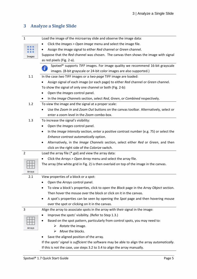
Load the array file (*.gal) and view the array data:

Click the Arrays > Open Array menu and select the array file.

The array (the white grid in Fig. 2) is then overlaid on top of the image in the canvas.

2.1 View properties of a block or a spot:

Open the Arrays control panel.

To view a block’s properties, click to open the Block page in the Array Object section.

Then hover the mouse over the block or click on it in the canvas.

A spot’s properties can be seen by opening the Spot page and then hovering mouse

over the spot or clicking on it in the canvas.

3

Align the array to associate spots in the array with their signal in the image:

Improve the spots’ visibility. (Refer to Step 1.3.)

Based on the spot pattern, particularly from control spots, you may need to:

Rotate the image.

Move the blocks.

Save the aligned position of the array.

If the spots’ signal is sufficient the software may be able to align the array automatically.

If this is not the case, use steps 3.2 to 3.4 to align the array manually.

3 | Analyze a Single Slide


3.1 To align the array automatically:

In the Array Object section, click the Align Array button.

You can check the array alignment result by increasing the signal’s visibility (Refer

to Step 1.3) and verifying if for all spots, the inner region bounded by the dashed

circle aligns well with the spot’s signal (green or red pixels, Fig. 2-b). If this is the

case, go directly to step 3.5 to save the aligned array.

3.2 To rotate the image:

In the Image Rotation section:

Flip horizontally and/or vertically.

Rotate images at angles of 90°, 180°, or 270°.

The rotated image can be saved to another file with the Images > Save Image As menu.

3.3 To select blocks containing spots that need reposition:

Open the Arrays control panel and then click on the Block page

To select individual blocks, click on them while pressing the Ctrl key.

Click Ctrl-A to select the entire array.

3.4 To move blocks:

Select blocks.

Click on the selection and drag the corresponding blocks to the intended position.

In the image, the spots’ signal is shown in red, green, or a color different from

white. Reposition the blocks such that for each spot, the inner region bounded by

the dashed circle is as close to the spot’s signal as possible (Fig. 2-b).

3.5 To save the aligned position of the array:

Choose the Arrays > Save Array menu to save the aligned array to the current file.

Save the aligned array to another GAL file using the Array > Save Array As menu.

4

Quantify the array data:

Make sure the array is correctly aligned with the image.

Click the Quantify button on the main toolbar to start the quantification procedure.

Upon finishing, the results are updated into the table of quantified data, each row

showing the intensity values of each spot. Suppose you assigned the image signal to

the Red channel, you may use the following values for finding spots of interest:

Red Foreground Mean or Red Foreground Median

If spot replication is employed: Aggregate Red Foreground Mean (or Median)

Quantification is a complex process which involves many concepts. If you would

like detailed information, please check the User’s Guide (Section 1.4 - Terms and

Concepts and Section 4 - Quantification of Microarray Data).

4.1 View the quantified data:

In the canvas, clicking on a spot shows the row in the table of quantified data that

contains the spot’s intensity values.

Alternatively, selecting a row in the table also highlights the associated spot in the

canvas. You can thus conveniently browse the quantified data with navigation keys

such as Up, Down, Page Up, and Page Down.

4 | Analyze many slides automatically


4.2

Observe hits with the scatter plot:

Click the Scatter Plot button on the main toolbar to display spots in a 2D-chart

according to their quantified data.

Select a block in the Blocks box in the Scatter Plot control panel to show only spots of

that block.

Use the blue bars to select hits which are spots whose intensity value is between the

bars’ value. Their data are then updated into the table below the chart.

Clicking on a hit in the chart highlights its row of data in the table. Conversely, select

a row in the table to highlight the corresponding spot.

4.3 Save the quantified data to a CSV file (*.csv) or GenePix Array Result file (*.gpr):

Click the Export to CSV File button or the Export to GPR File button, respectively.

4.4 Save the analysis results:

Choose the Project > Save Project menu to save the analysis results to a Spotxel®

project file (*.spotxelproj).

The project file, e.g. named s1.spotxelproj, contains the path to the image, the

aligned array, and the quantified data. When later opening s1.spotxelproj with the

Project > Open Project menu, the image, the aligned array, as well as the quantified

data will be reloaded.

4 Analyze many slides automatically

Suppose that the study is to screen a protein microarray with k samples. This employs k slides of the

protein microarray whose annotation is based on a single GAL file, the so-called template array. The

screening of k slides results in k scanned images. You can then setup a batch to automatically process

all k images and generate their quantified data.

The images are either one-page or two-page grayscale TIFF file. For correct array alignment, the

spots’ signal in the images should be sufficient for positioning the array.

1

Create and execute the batch:

Click the Batch button on the main toolbar to create a new batch.

In the Batch control panel, specify the images, the template array, and the options.

Execute the batch.

1.1 To specify parameters and options of the batch:

Click the Add button and select the images for processing.

Double-click on the Template array edit-box and browse to the template array file.

Specify the folder to store generated files.

Finally, save the batch to a file using the Batch > Save Batch menu. The batch log is

created automatically and named after the batch file.

For each batch, we recommend using a separate folder to store the batch file and

generated data files.



1.2 Execute the batch:

Click the Run button to start the batch. During execution, the status of the currently

processed images will be updated.

Suppose that sample001.tif is an image in the batch. The following data files are then

generated for this image:

sample001.gal: the array file in which the array’s spots are associated with their

signal in the image sample001.tif,

sample001.csv: the CSV file containing only the quantified data,

sample001.gpr: the file containing quantified data in GenePix Result format, and

sample001.spotxelproj: the project file containing the analysis data for the image.

As a result, k project files (*.spotxelproj) will be generated for a batch of k images. They

can be used for further processing described in the next steps.

2

Process replicates, filtering data, and normalize data:

Click the Norm button on the main toolbar.

In the Dataset Files panel:

Click the Load button and select the k project files (*.spotxelproj).

Select a screening value in the Data column list-box, e.g. Red Foreground

Mean or Red Foreground Median.

2.1 To consolidate replicates’ signal value with the Replicate Processing panel:

At the Unique header list-box, select a suitable header such as Name.

Click the Process button.

The processed dataset is then shown in the Replicate Processing table.

2.2 To filter a dataset using keywords and thresholds with the Data Filtering panel:

First, select the dataset by clicking on its table. If there is more than one table, the

selected one is highlighted with green border.

Select Contains, Excludes, or Regular expression. Enter one or more keywords, or the

search pattern, into the corresponding textbox. Press Enter. The data is directly in

the currently selected table.

Use the sliders or enter a number directly to set the lower and upper thresholds.

2.3 To normalize the data with the Data Normalization panel:

First, select the dataset by clicking on its table.

Choose to normalize with Z-Score, Z-Factor, or ratio to mean value of controls. In the

two latter cases, click the Select Controls button and specify the controls.

Click the Normalize button. The normalized data is then shown in the table titled

Normalized Dataset.

2.4 Iteratively optimize the dataset:

Replicate processing (2.1), data filtering (2.2), and data normalization (2.3) can be

applied many times. Simply select the table containing the dataset first.

Use the Export button in Dataset Files panel to export the selected dataset to a CSV

file, e.g., for PCA or HCA analysis.

Use the Window > Tile or Window > Cascade menu to arrange the datasets.



In addition to Spotxel® project files (*.spotxelproj), the tool also accepts a list of

GenePix Result files (*.gpr) or a CSV file prepared in the suitable dataset format.

For detailed steps on the dataset and the PCA tool, refer to Section 7.1 – Datasets -

and Section 7 - Data Preprocessing and Normalization - of the User’s Guide.

3

Identify important proteins and samples with Principal Component Analysis (PCA):

Click the PCA button on the main toolbar.

In the PCA control panel:

Click the Load Data button and select the k project files (*.spotxelproj).

Select a screening value in the Data Column list-box, e.g. Red Foreground


3.1 To find proteins that influence the variance of the study:

Choose Simplify the dataset to three Samples.

Click the Start Analysis button.

3.2 To find samples that influence the variance of the study:

Choose Simplify the dataset to three Features.


For detailed steps on the dataset and the PCA tool, refer to Section 7.1 – Datasets -

and Section 8.1 - Principal Component Analysis - of the User’s Guide.

4

Discover relationships between proteins and samples with Hierarchical Clustering

Analysis (HCA):

Click the HC button on the main toolbar.

In the HCA control panel:

Click the Load Data button and select the k project files (*.spotxelproj).

Select a screening value in the Data Column list-box, e.g. Red Foreground


Choose to construct the clustering tree for features (i.e. proteins), or

samples, or both of them.


The Hierarchical Clustering sheet then shows a heat map. It is like a matrix of boxes with

rows representing proteins and columns representing samples. Consider the box at row p

and column s, its color represents the screening value of protein p against sample s.

In addition, samples that are related (e.g. those that response similarly to a certain group

of proteins) are grouped into a cluster. Their relationship is illustrated by a line

connecting them. The clusters of proteins are similarly depicted.

4.1 To review the screening result of protein p against sample s:

Observe the color of the corresponding box on the heat map.

4.2 To identify the relationship between proteins or between samples:

Observe the clusters and the line connecting them.

For detailed steps on the dataset and the HCA tool, refer to Section 7.1 – Datasets -

and Section 8.2 - Hierarchical Clustering Analysis - of the User’s Guide.

spotxel® 1.7 microarray image and data analysis software

Documents