Sprinklers: A Randomized Variable-Size Striping Approach to

Reordering-Free Load-Balanced Switching

Weijun Ding ∗ Jim Xu † Jim Dai‡ Yang Song§ Bill Lin¶

June 7, 2014

Abstract

Internet traffic continues to grow exponentially, calling for switches that can scale well inboth size and speed. While load-balanced switches can achieve such scalability, they suffer froma fundamental packet reordering problem. Existing proposals either suffer from poor worst-casepacket delays or require sophisticated matching mechanisms. In this paper, we propose a newfamily of stable load-balanced switches called “Sprinklers” that has comparable implementationcost and performance as the baseline load-balanced switch, but yet can guarantee packet or-dering. The main idea is to force all packets within the same virtual output queue (VOQ) totraverse the same “fat path” through the switch, so that packet reordering cannot occur. Atthe core of Sprinklers are two key innovations: a randomized way to determine the “fat path”for each VOQ, and a way to determine its “fatness” roughly in proportion to the rate of theVOQ. These innovations enable Sprinklers to achieve near-perfect load-balancing under arbi-trary admissible traffic. Proving this property rigorously using novel worst-case large deviationtechniques is another key contribution of this work.

1 Introduction

Internet service providers need high-performance switch architectures that can scale well in bothsize and speed, provide throughput guarantees, achieve low latency, and maintain packet ordering.However, conventional crossbar-based switch architectures with centralized scheduling and arbitraryper-packet dynamic switch configurations are not scalable.

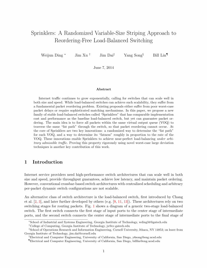
An alternative class of switch architecture is the load-balanced switch, first introduced by Changet al. [2, 3], and later further developed by others (e.g. [9, 11, 13]). These architectures rely on twoswitching stages for routing packets. Fig. 1 shows a diagram of a generic two-stage load-balancedswitch. The first switch connects the first stage of input ports to the center stage of intermediateports, and the second switch connects the center stage of intermediate ports to the final stage of

∗School of Industrial and Systems Engineering, Georgia Institute of Technology, wding34@gatech.edu†College of Computing, Georgia Institute of Technology, jx@cc.gatech.edu‡School of Operations Research and Information Engineering, Cornell University, Ithaca, NY 14853; on leave from

Georgia Institute of Technology, jim.dai@cornell.edu§Electrical and Computer Engineering, University of California, San Diego, y6song@eng.ucsd.edu¶Electrical and Computer Engineering, University of California, San Diego, billlin@eng.ucsd.edu

1

output ports. Both switching stages execute a deterministic connection pattern such that each inputto a switching stage is connected to each output of the switch at 1/Nth of the time. This can beimplemented for example using a deterministic round-robin switch (see Sec. 3.4). Alternatively, asshown in [11], the deterministic connection pattern can also be efficiently implemented using opticsin which all inputs are connected to all outputs of a switching stage in parallel at a rate of 1/Nththe line rate. This class of architectures appears to be a practical way to scale high-performanceswitches to very high capacities and line rates.

1

2

N

.

.

.

1

2

N

.

.

.

1

2

N

.

.

.

Inputs Outputs Intermediate 1st Stage Switch

2nd Stage Switch

Figure 1: Generic load-balanced switch.

Although the baseline load-balanced switch originally proposed in [2] is capable of achievingthroughput guarantees, it has the critical problem that packet departures can be badly out-of-order. In the baseline load-balanced switch, consecutive packets at an input port are spread toall N intermediate ports upon arrival. Packets going through different intermediate ports mayencounter different queueing delays. Thus, some of these packets may arrive at their output portsout-of-order. This is detrimental to Internet traffic since the widely used TCP transport proto-col falsely regards out-of-order packets as indications of congestion and packet loss. Therefore, anumber of researchers have explored this packet ordering problem (e.g. [9, 11, 13]).

1.1 Our approach

In this paper, we propose “Sprinklers,” a new load-balanced switching solution that has comparableimplementation cost and computational complexity, and similar performance guarantees as thebaseline load-balanced switch, yet can guarantee packet ordering. The Sprinklers approach has amild flavor of a simple, yet flawed solution called “TCP hashing”1 [11]. The idea of TCP hashing isto force all packets at an input port that belong to the same application (TCP or UDP) flow to gothrough the same randomly chosen intermediate port by hashing on the packet’s flow identifier. Thisapproach ensures that all packets that belong to the same application flow will depart the switchin order because they will encounter the same queueing delay through the same intermediate port.Although the TCP hashing scheme is simple and intuitive, it cannot guarantee stability because anintermediate port can easily be oversubscribed by having too many large flows randomly assignedto it.

Like the TCP hashing approach in which all packets within an application flow are forced to gothrough the same switching path, a Sprinklers switch requires all packets within a Virtual OutputQueue (VOQ) to go down the same “fat path” called a stripe. Specifically, for each VOQ, aSprinklers switch stripes packets within a VOQ across an interval of consecutive intermediate ports,

1TCP hashing is referred to as “Application Flow Based Routing” (AFBR) in [11].

2

which we call a stripe interval. The number of intermediate ports L in the stripe interval is referredto as its size. In the Sprinklers approach, the size L of the stripe interval is determined roughly inproportion to the rate of the VOQ, and the placement of the L consecutive intermediate ports is bymeans of random permutation. Therefore, the N2 stripe intervals, corresponding to the N2 VOQsat the N input ports, can be very different from one another in both sizes and placements. Theplacement of variable-size stripes by means of random permutation ensures that the traffic loadsassociated with them get evenly distributed across the N intermediate ports.

For example, suppose a VOQ is assigned to the stripe interval (8, 12] based on its arrival rate andrandom permutation, which corresponds to intermediate ports {9, 10, 11, 12}. Then the incomingpackets belonging to this VOQ will be grouped in arrival order into stripes of L = 4 packets each.Once a stripe is filled, the L = 4 packets in the stripe will be transmitted to intermediate ports 9,10, 11, and 12, respectively.

By making a stripe the basic unit of scheduling at both input and intermediate ports, a Sprinklersswitch ensures that every stripe of packets departs from its input port and arrives at its output portboth “in one burst” (i.e., in consecutive time slots). This “no interleaving between the servicing oftwo stripes” service guarantee, combined with the FCFS order in which packets within a stripe andstripes within a VOQ are served, ensures that packet reordering cannot happen within any VOQ,and hence cannot happen within any application flow either.

1.2 Contributions of the paper

This paper makes the following major contributions:

• First, we introduce the design of a new load-balanced switch architecture based on randomizedand variable-size striping that we call Sprinklers. Sprinklers is indeed scalable in that all itsalgorithmic aspects can be implemented in constant time at each input port and intermediateport in a fully distributed manner.

• Second, we develop novel large deviation techniques to prove that Sprinklers is stable underintensive arrival rates with overwhelming probability, while guaranteeing packet order.

• Third, to our knowledge, Sprinklers is the first load-balanced switch architecture based onrandomization that can guarantee both stability and packet ordering, which we hope will be-come the catalyst to a rich family of solutions based on the simple principles of randomizationand variable stripe sizing.

1.3 Outline of the paper

The rest of the paper is organized as follows. Sec. 2 provides a brief review of existing load-balancedswitch solutions. Sec. 3 introduces the structure of our switch and explains how it works. Sec. 4provides a rigorous proof of stability based on the use of convex optimization theory and negativeassociation theory to develop a Chernoff bound for the overload probability. This section alsopresents our worst-case large deviation results. Sec. 6 evaluates our proposed architecture, andSec. 7 concludes the paper.

3

2 Existing Load-Balanced Switch Solutions

2.1 Hashing-Based

As discussed in Sec. 1, packets belonging to the same TCP flow can be guaranteed to depart fromtheir output port in order if they are forced to go through the same intermediate port. The selectionof intermediate port can be easily achieved by hashing on the packet header to obtain a value from1 to N . Despite its simplicity, the main drawback of this TCP hashing approach is that stabilitycannot be guaranteed [11].

2.2 Aggregation-Based

An alternative class of algorithms to hashing is based on aggregation of packets into frames. Oneapproach called Uniform Frame Spreading (UFS) [11] prevents reordering by requiring that eachinput first accumulates a full-frame of N packets, all going to the same output, before uniformlyspreading the N packets to the N intermediate ports. Packets are accumulated in separate virtualoutput queues (VOQs) at each input for storing packets in accordance to their output. When afull-frame is available, the N packets are spread by placing one packet at each of the N intermediateports. This ensures that the lengths of the queues of packets destined to the same output are thesame at every intermediate port, which ensures every packet going to the same output experiencesthe same queuing delay independent of the path that it takes from input to output. Although ithas been shown in [11] that UFS achieves 100% throughput for any admissible traffic pattern, themain drawback of UFS is that it suffers from long delays, O(N3) delay in the worst-case, due tothe need to wait for a full-frame before transmission. The performance of UFS is particularly badat light loads because slow packet arrivals lead to much longer accumulation times.

An alternative aggregation-based algorithm that avoids the need to wait for a full-frame is calledFull Ordered Frames First (FOFF) [11]. As with UFS, FOFF maintains VOQs at each input.Whenever possible, FOFF will serve full-frames first. When there is no full-frame available, FOFFwill serve the other queues in a round-robin manner. However, when incomplete frames are served,packets can arrive at the output out of order. It has been shown in [11] that the amount ofreordering is always bounded by O(N2) with FOFF. Therefore, FOFF adds a reordering bufferof size O(N2) at each output to ensure that packets depart in order. It has been shown in [11]that FOFF achieves 100% throughput for any admissible traffic pattern, but the added reorderingbuffers lead to an O(N2) in packet delays.

Another aggregation-based algorithm called Padded Frames (PF) [9] was proposed to avoid theneed to accumulate full-frames. Like FOFF, whenever possible, FOFF will serve full-frames first.When no full-frame is available, PF will search among its VOQ at each input to find the longestone. If the length of the longest queue exceeds some threshold T , PF will pad the frame with fakepackets to create a full-frame. This full-frame of packets, including the fake packets, are uniformlyspread across the N intermediate ports, just like UFS. It has been shown in [9] that PF achieves100% throughput for any admissible traffic pattern, but its worst-case delay bound is still O(N3).

2.3 Matching-Based

Finally, packet ordering can be guaranteed in load-balanced switches via another approach called aConcurrent Matching Switch (CMS) [13]. Like hashing-based and aggregation-based load-balanced

4

switch designs, CMS is also a fully distributed solution. However, instead of bounding the amountof packet reordering through the switch, or requiring packet aggregation, a CMS enforces packetordering throughout the switch by using a fully distributed load-balanced scheduling approach.Instead of load-balancing packets, a CMS load-balances request tokens among intermediate ports,where each intermediate port concurrently solves a local matching problem based only on its localtoken count. Then, each intermediate port independently selects a VOQ from each input to serve,such that the packets selected can traverse the two load-balanced switch stages without conflicts.Packets from selected VOQs depart in order from the inputs, through the intermediate ports, andfinally through the outputs. Each intermediate port has N time slots to perform each matching,so the complexity of existing matching algorithms can be amortized by a factor of N .

3 Our scheme

Sprinklers has the same architecture as the baseline load-balanced switch (see Fig. 1), but it differsin the way that it routes and schedules packets for service at the input and intermediate ports. Also,Sprinklers have N VOQs at each input port. In this section, we first provide some intuition behindthe Sprinklers approach, followed by how the Sprinklers switch operates, including the stripingmechanism for routing packets through the switch and the companion stripe scheduling policy.

3.1 Intuition Behind the Sprinklers Approach

The Sprinklers approach is based on three techniques for balancing traffic evenly across all N inter-mediate ports: permutation, randomization, and variable-size striping. To provide some intuitionas to why all three techniques are necessary, we use an analogy from which the name Sprinklersis derived. Consider the task of watering a lawn consisting of N identically sized areas using Nsprinklers with different pressure. The objective is to distribute an (ideally) identical amount ofwater to each area. This corresponds to evenly distributing traffic inside the N VOQs (sprinklers)entering a certain input port to the N intermediate ports (lawn areas) under the above-mentionedconstraint that all traffic inside a VOQ must go through the same set of intermediate ports (i.e.,the stripe interval) to which the VOQ is mapped.

An intuitive and sensible first step is to aim exactly one sprinkler at each lawn area, since aimingmore than one sprinklers at one lawn area clearly could lead to it being flooded. In other words, the“aiming function,” or “which sprinkler is aimed at which lawn area,” is essentially a permutationover the set {1, 2, · · · , N}. This permutation alone however cannot do the trick, because the waterpressure (traffic rate) is different from one sprinkler to another, and the lawn area aimed at bya sprinkler with high water pressure will surely be flooded. To deal with such disparity in waterpressures, we set the “spray angle range” of a sprinkler, which corresponds to the size (say L)of the stripe interval for the corresponding VOQ, proportional to its water pressure, and evenlydistribute this water pressure across the L “streams” of water that go to the target lawn area andL− 1 “neighboring” lawn areas.

However, such water pressure equalization (i.e., variable stripe sizing) alone does not prevent allscenarios of load-imbalance because it shuffles water around only “locally.” For example, if a largerthan average number of high pressure sprinklers are aimed at a cluster of lawn areas close to oneanother, some area within this cluster will be flooded. Hence, a simple yet powerful randomized

5

algorithm is brought in to shuffle water around globally: we simply sample this permutation atuniform random from the set of all N ! permutations.

Besides load-balancing, there is another important reason for the size of a stripe interval to be setroughly proportional to the traffic rate of the corresponding VOQ. In some existing solutions tothe packet reordering problem with load-balanced switches, each VOQ has to accumulate a fullframe of N packets before the frame can depart from the input port. For a VOQ with low trafficrate, this buffering delay could be painfully long. By adopting rate-proportional stripe sizing, aSprinklers switch significantly reduces the buffering delays experienced by the low-rate VOQs.

As far as the Sprinklers analogy goes, the combination of randomized permutation and waterpressure equalization, with proper “manifoldization” (i.e., considering N + 1 as 1), will provablyensure that the amount of water going to each lawn area is very even with high probability. However,because the servicing of any two stripes cannot interleave in a Sprinklers switch (to ensure correctpacket order), two stripes have to be serviced in two different frames (N time slots), even if theirstripe intervals overlap only slightly. A rampant occurrence of such slight overlaps, which canhappen if the stripe interval size of a VOQ is set strictly proportional to the rate of the VOQ(rounded to an integer), will result in gross waste of service capacity, and significantly reduce themaximum achievable throughput.

Therefore, we would like any two stripe intervals to either “bear hug” (i.e., one contained entirelyin the other) or does not touch (no overlap between the intervals) each other. Our solution is aclassical “computer science” one: making N a power of 2 (very reasonable in the modern switchingliterature) and every stripe interval a dyadic one (resulting from dividing the whole interval (0,N] into 2k equal-sized subintervals for an integer k ≤ log2N). Now that the spray angle range ofa sprinkler has to be a power of 2, the water pressure per stream could vary from one sprinklerto another by a maximum factor of 2. However, as shown later in Sec. 4, strong statistical load-balancing guarantees can still be rigorously proven despite such variations.

3.2 Operations of the Sprinklers Switch

As just explained, traffic inside each of the N2 VOQs is switched through a dyadic interval ofintermediate ports that is just large enough to bring the load imposed by the VOQ on any in-termediate port within this interval (i.e., “water pressure per stream”) below a certain threshold.The sizes of the corresponding N2 stripe intervals are determined by the respective rates of thecorresponding VOQs, and their placements to consecutive intermediate ports are performed using arandomized algorithm. Once generated, their placements remain fixed thereafter, while their sizescould change when their respective rates do. Our goal in designing this randomized algorithm isthat, when switched through the resulting (random) stripe intervals, traffic going out of any inputport or going into any output port is near-perfectly balanced across all N intermediate ports, withoverwhelming probabilities.

Once the N2 stripe intervals are generated and fixed, packets in each VOQ will be striped acrossits corresponding interval of intermediate ports as follows. Fix an arbitrary VOQ, and let its stripesize and interval be 2k and (`, `+ 2k] ≡ {`+ 1, `+ 2, · · · , `+ 2k}, respectively. (The integer ` mustbe divisible by 2k for the interval to be dyadic, as discussed earlier.) Packets in this VOQ aredivided, chronologically according to their arrival times, into groups of 2k packets each and, with aslight abuse of the term, we refer to each such group also as a stripe. Such a stripe will eventuallybe switched through the set of intermediate ports {` + 1, ` + 2, · · · , ` + 2k} as follows. Assume

6

this switching operation starts at time (slot) t, when the corresponding input port is connected tothe intermediate port ` + 1 by the first switching fabric. Then, following the periodic connectionsequence of the first switching fabric, the input port forwards the first packet in the stripe to theintermediate port ` + 1 at time t, the second packet to the intermediate port ` + 2 at time t + 1,and so on, until it forwards the last packet in the stripe to the intermediate port ` + 2k at timet+ 2k− 1. That is, packets in this stripe go out of the input port to consecutive intermediate portsin consecutive time slots (i.e., “continuously”). The same can be said about other stripes fromthis and other VOQs. This way, at each input port, the (switching) service is rendered by the firstswitching fabric in a stripe-by-stripe manner (i.e., finish serving one stripe before starting to serveanother).

At each input port, packets from the N VOQs originated from it compete for (the switching)service by the first switching fabric and hence must be arbitrated by a scheduler. However, sincethe service is rendered stripe-by-stripe, as explained above, the scheduling is really performed amongthe competing stripes. In general, two different scheduling policies are needed in a Sprinklers switch,one used at the input ports and the other at intermediate ports. Designing stripe scheduling policiesthat are well suited for a Sprinklers switch turns out to be a difficult undertaking because two trickydesign requirements have to be met simultaneously.

The first requirement is that the resulting scheduling policies must facilitate a highly efficientutilization of the switching capacity of both switching fabrics. To see this, consider input port i,whose input link has a normalized rate of 1, and intermediate port `. As explained in Sec. 1, thesetwo ports are connected only once every N time slots, by the first switching fabric. Consider theset of packets at input port i that needs to be switched to the intermediate port `. This set canbe viewed and called a queue (a queueing-theoretic concept), because the stripe scheduling policynaturally induces a service order (and hence a service process) on this set of packets, and the arrivaltime of each packet is simply that of the stripe containing the packet. Clearly, the service rate ofthis queue is exactly 1/N . Suppose this input port is heavily loaded say with a normalized arrivalrate of 0.95. Then even with perfect load-balancing, the arrival rate to this queue is 0.95/N , onlyslightly below the service rate 1/N . Clearly, for this queue to be stable, there is no room for anywaste of this service capacity. In other words, the scheduling policy must be throughput optimal.

The second requirement is exactly why we force all packets in a VOQ to go down the same fatpath (i.e., stripe interval) through a Sprinklers switch, so as to guarantee that no packet reorderingcan happen. It is easy to verify that for packet order to be preserved within every stripe (andhence within every VOQ), it suffices to guarantee that packets in every stripe go into their destina-tion output port from consecutive intermediate ports in consecutive time slots (i.e., continuously).However, it is much harder for a stripe of 2k packets to arrive at an output port continuously (thanto leave an input port), because these packets are physically located at a single input port whenthey leave the input port, but across 2k different intermediate ports right before they leave for theoutput port.

After exploring the entire space of stripe-by-stripe scheduling policies, we ended up adopting thesame stripe scheduling policy, namely Largest Stripe First (LSF), at both input ports and inter-mediate ports, but not for the same set of reasons. At input ports, LSF is used because it isthroughput optimal. At intermediate ports, LSF is also used because it seems to be the only policythat makes every stripe of packets arrive at their destination output port continuously withoutincurring significant internal communication costs between the input and intermediate ports. InSec. 3.4, we will describe the LSF policies at the input and intermediate ports.

7

3.3 Generating Stripe Intervals

As we have already explained, the random permutation and the variable dyadic stripe sizing tech-niques are used to generate the stripe intervals for the N VOQs originated from a single inputport, with the objective of balancing the traffic coming out of this input port very evenly across allN intermediate ports. In Sec. 3.3.1, we will specify this interval generating process precisely andprovide detailed rationales for it. In Sec. 3.3.2, we will explain why and how the interval generatingprocesses at N input ports should be carefully coordinated.

3.3.1 Stripe interval generation at a single input port

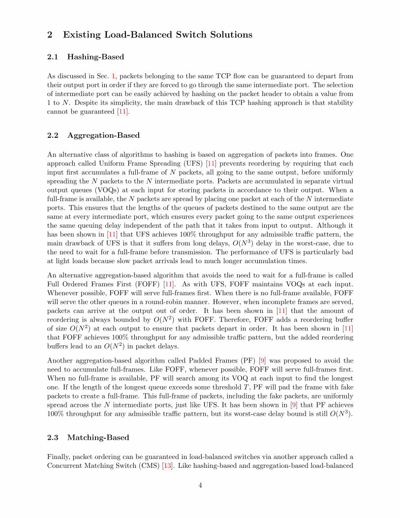
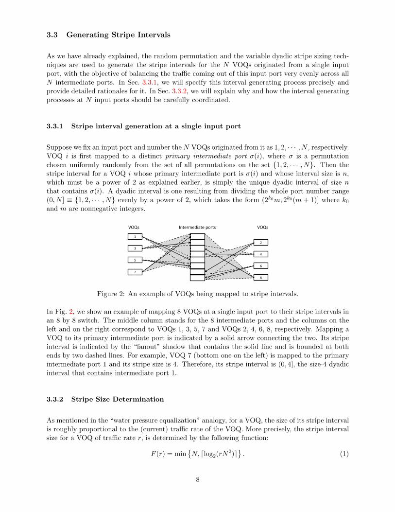
Suppose we fix an input port and number theN VOQs originated from it as 1, 2, · · · , N , respectively.VOQ i is first mapped to a distinct primary intermediate port σ(i), where σ is a permutationchosen uniformly randomly from the set of all permutations on the set {1, 2, · · · , N}. Then thestripe interval for a VOQ i whose primary intermediate port is σ(i) and whose interval size is n,which must be a power of 2 as explained earlier, is simply the unique dyadic interval of size nthat contains σ(i). A dyadic interval is one resulting from dividing the whole port number range(0, N ] ≡ {1, 2, · · · , N} evenly by a power of 2, which takes the form (2k0m, 2k0(m + 1)] where k0

and m are nonnegative integers.

1

3

5

7

2

4

6

8

Intermediate ports VOQs VOQs

Figure 2: An example of VOQs being mapped to stripe intervals.

In Fig. 2, we show an example of mapping 8 VOQs at a single input port to their stripe intervals inan 8 by 8 switch. The middle column stands for the 8 intermediate ports and the columns on theleft and on the right correspond to VOQs 1, 3, 5, 7 and VOQs 2, 4, 6, 8, respectively. Mapping aVOQ to its primary intermediate port is indicated by a solid arrow connecting the two. Its stripeinterval is indicated by the “fanout” shadow that contains the solid line and is bounded at bothends by two dashed lines. For example, VOQ 7 (bottom one on the left) is mapped to the primaryintermediate port 1 and its stripe size is 4. Therefore, its stripe interval is (0, 4], the size-4 dyadicinterval that contains intermediate port 1.

3.3.2 Stripe Size Determination

As mentioned in the “water pressure equalization” analogy, for a VOQ, the size of its stripe intervalis roughly proportional to the (current) traffic rate of the VOQ. More precisely, the stripe intervalsize for a VOQ of traffic rate r, is determined by the following function:

F (r) = min{N, dlog2(rN2)e

}. (1)

8

The stripe size determination rule (1) tries to bring the amount of traffic each intermediate portwithin the stripe interval receives from this VOQ below 1/N2 while requiring that the stripe sizebe a power of 2. However, if the rate r is very high, say > 1

N , then the stripe size F (r) is simplyN .

The initial sizing of the N2 stripe intervals may be set based on historical switch-wide trafficmatrix information, or to some default values. Afterwards, the size of a stripe interval will beadjusted based on the measured rate of the corresponding VOQ. To prevent the size of a stripefrom “thrashing” between 2k and 2k+1, we can delay the halving and doubling of the stripe size.Although our later mathematical derivations assume the perfect adherence to the above stripe sizedetermination rule, the change in the provable load-balancing guarantees is in fact negligible whena small number of stripe sizes are a bit too small (or too large) for the respective rates of theircorresponding VOQs.

3.3.3 Coordination among all N2 stripe intervals

Like an input port, an output port is connected to each intermediate port also exactly once everyN time slots, and hence needs to near-perfectly balance the traffic load coming into it. That is,roughly 1

N of that load should come from each intermediate port. In this section, we show how toachieve such load balancing at an output port, by a careful coordination among the (stripe-interval-generating) permutations σi, i = 1, 2, · · · , N .

Now consider an arbitrary output port j. There are precisely N VOQs destined for it, one originatedfrom each input port. Intuitively, they should ideally be mapped (permuted) to N distinct primaryintermediate ports – for the same reason why the N VOQs originated from an input port aremapped (permuted) to N distinct primary intermediate ports – by the permutations σ1, σ2, · · · ,σN , respectively. We will show this property holds for every output port j if and only if the matrixrepresentation of these permutations is an Orthogonal Latin Square (OLS).

Consider an N ×N matrix A = (aij), i, j = 1, 2, · · · , N , where aij = σi(j). Consider the N VOQsoriginated at input port i, one destined for each output port. We simply number each VOQ byits corresponding output port. Clearly row i of the matrix A is the primary intermediate portsof these N VOQs. Now consider the above-mentioned N VOQs destined for output port j, oneoriginated from each input port. It is easy see that the jth column of matrix A, namely σ1(j),σ2(j), · · · , σN (j), is precisely the primary intermediate ports to which these N VOQs are mapped.As explained earlier, we would like these numbers also to be distinct, i.e., a permutation of theset {1, 2, · · · , N}. Therefore, every row or column of the matrix A must be a permutation of{1, 2, · · · , N}. Such a matrix is called an OLS in the combinatorics literature [4].

Our worst-case large deviation analysis in Sec. 4 requires the N VOQs at the same input port ordestined to the same output port select their primary intermediate ports according to a uniformrandom permutation. Mathematically, we only require the marginal distribution of the permutationrepresented by each row or column of the OLS A to be uniform. The use of the word “marginal”here emphasizes that we do not assume any dependence structure, or the lack thereof, amongthe N random permutations represented by the N rows and among those represented by the Ncolumns. We refer to such an OLS as being weakly uniform random, to distinguish it from anOLS sampled uniformly randomly from the space of all OLS’ over the alphabet set {1, 2, · · · , N},which we refer to as being strongly uniform random. This distinction is extremely important for us,since whether there exists a polynomial time randomized algorithm for generating an OLS that is

9

approximately strongly uniform random has been an open problem in theoretical computer scienceand combinatorics for several decades [6, 8]. A weakly uniform random OLS, on the other hand,can be generated in O(N logN) time, shown as following.

We first generate two uniform random permutations σ(R) and σ(C) over the set {1, 2, · · · , N} thatare mutually independent, using a straightforward randomized algorithm [7]. This process, whichinvolves generating log2N ! = O(N logN) random bits needed to “index” σ(R) and σ(C) each, hasO(N logN) complexity in total. Then each matrix element a(i, j) is simply set to (σ(R)(i)+σ(C)(j)mod N) + 1. It is not hard to verify that each row or column is a uniform random permutation.

3.4 Largest Stripe First Policy

In this section, we describe our stripe scheduling policy called Largest Stripe First (LSF), which isused at both input and intermediate ports of a Sprinklers switch. LSF can be implemented in astraightforward manner, at both input and intermediate ports, using N(log2N + 1) FIFO queues(a data structure concept). Using an N × (log2N + 1) 2D-bitmap to indicate the status of eachqueue (0 for empty, 1 for nonempty), the switch can identify the rightmost bit set in each row ofthe bitmap in constant time, which is used by LSF to identify the largest stripe to serve at eachport.

We first provide a brief description of the periodic sequences of connections executed at bothswitching fabrics shown in Fig. 1. The first switching fabric executes a periodic “increasing”sequence, that is, at any time slot t, each input port i is connected to the intermediate port ((i+ t)mod N) + 1. The second switching fabric, on the other hand, will execute a periodic “decreasing”sequence, that is, at any time slot t, each intermediate port ` is connected to the output port ((`−t)mod N) + 1.

In the rest of the paper, we make the following standard homogeneity assumption about a Sprinklersswitch. Every input, intermediate, or output port operates at the same speed. That is, each canprocess and transmit exactly one packet per time slot. We refer to this speed as 1. Every connectionmade in a switching fabric also has speed of 1 (i.e., one packet can be switched per time slot). SinceN connections are made by a switching fabric at any time slot, up to N packets can be switchedduring the time slot.

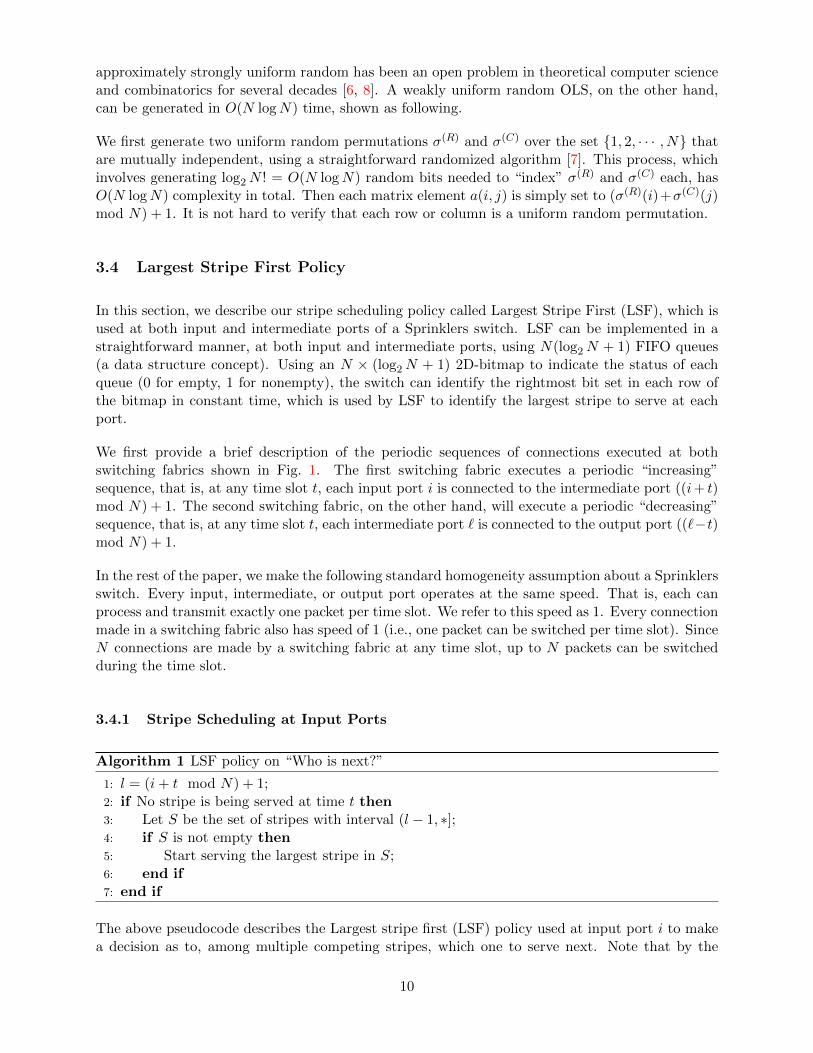
3.4.1 Stripe Scheduling at Input Ports

Algorithm 1 LSF policy on “Who is next?”

1: l = (i+ t mod N) + 1;2: if No stripe is being served at time t then3: Let S be the set of stripes with interval (l − 1, ∗];4: if S is not empty then5: Start serving the largest stripe in S;6: end if7: end if

The above pseudocode describes the Largest stripe first (LSF) policy used at input port i to makea decision as to, among multiple competing stripes, which one to serve next. Note that by the

10

stripe-by-stripe nature of the scheduler, it is asked to make such a policy decision only when itcompletely finishes serving a stripe. The policy is simply to pick among the set of stripes whosedyadic interval starts at intermediate port ` – provided that the set is nonempty – the largestone (FCFS for tie-breaking) to start serving immediately. The LSF policy is clearly throughputoptimal because it is work-conserving in the sense whenever a connection is made between inputport i and intermediate port `, a packet will be served if there is at least one stripe at the inputport whose interval contains `. Using terms from queueing theory [12] we say this queue is servedby a work-conserving server with service rate 1/N .

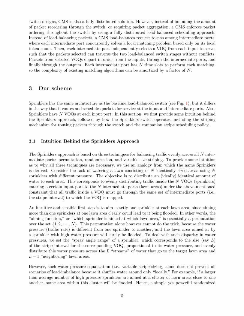
A stripe service schedule, which is the outcome of a scheduling policy acting on the stripe arrivalprocess, is represented by a schedule grid, as shown in Fig. 3. There are N rows in the grid, eachcorresponding to an intermediate port. Each tiny square in the column represents a time slot.The shade in the square represents a packet scheduled to be transmitted in that slot and differentshade patterns mean different VOQs. Hence each “thin vertical bar” of squares with the sameshade represents a stripe in the schedule. The time is progressing on the grid from right to left inthe sense that packets put inside the rightmost column will be served in the first cycle (N timeslots), the next column to the left in the second cycle, and so on. Within each column, time isprogressing from up to down in the sense that packet put inside the uppermost cell will be switchedto intermediate port 1 say at time slot t0, packet put inside the cell immediately below it will beswitched to intermediate port 2 at time slot t0 + 1, and so on. Note this up-down sequence isconsistent with the above-mentioned periodic connection pattern between the input port and theintermediate ports. Therefore, the scheduler is “peeling” the grid from right to left and from up todown.

For example, Fig. 3 corresponds to the statuses of the scheduling grid at time t0 and t0 + 8, whereLSF is the scheduling policy. We can see that the rightmost column in the left part of Fig. 3,representing a single stripe of size 8, is served by the first switching fabric in the meantime, andhence disappears in the right part of the figure. The above-mentioned working conservation natureof the LSF server for any input port is also clearly illustrated in Fig. 3: There is no “hole” in anyrow.

𝑡 = 𝑡0 𝑡 = 𝑡0+8

Figure 3: Statuses of the stripe scheduling at time t0 (left) and t0 + 8 (right) respectively.

While the scheduler always peels the grid from right to left and from up to down, the schedulermay insert a stripe ahead of other stripes smaller than it in size. In this case, the planned servicetime of all cells and bars to the left of the inserted vertical bar are shifted to the left by 1 column,meaning that their planned service time will be delayed by N time slots. For example, we can seefrom comparing the two parts of Fig. 3 that a stripe of size 4 is inserted in the lower part of the 3rdcolumn in the right part of Fig. 3, after two other stripes of size 4, but before some other stripesof smaller sizes.

11

3.4.2 Implementation of LSF at an Input Port

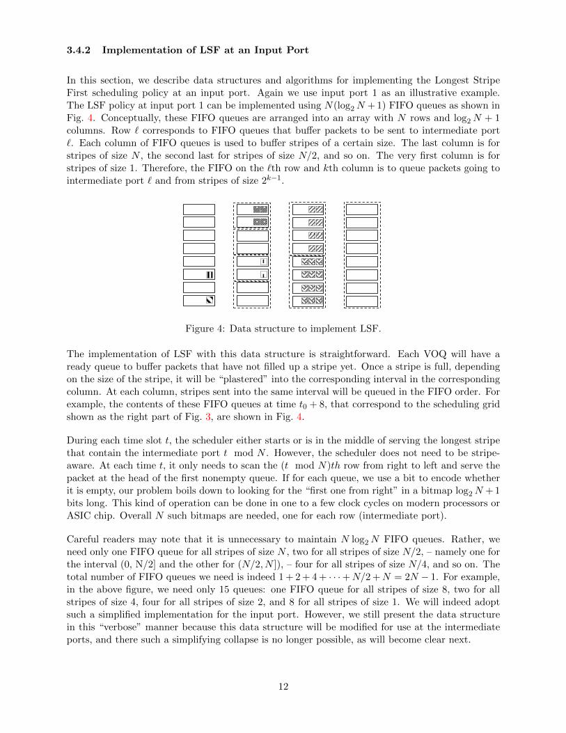
In this section, we describe data structures and algorithms for implementing the Longest StripeFirst scheduling policy at an input port. Again we use input port 1 as an illustrative example.The LSF policy at input port 1 can be implemented using N(log2N + 1) FIFO queues as shown inFig. 4. Conceptually, these FIFO queues are arranged into an array with N rows and log2N + 1columns. Row ` corresponds to FIFO queues that buffer packets to be sent to intermediate port`. Each column of FIFO queues is used to buffer stripes of a certain size. The last column is forstripes of size N , the second last for stripes of size N/2, and so on. The very first column is forstripes of size 1. Therefore, the FIFO on the `th row and kth column is to queue packets going tointermediate port ` and from stripes of size 2k−1.

Figure 4: Data structure to implement LSF.

The implementation of LSF with this data structure is straightforward. Each VOQ will have aready queue to buffer packets that have not filled up a stripe yet. Once a stripe is full, dependingon the size of the stripe, it will be “plastered” into the corresponding interval in the correspondingcolumn. At each column, stripes sent into the same interval will be queued in the FIFO order. Forexample, the contents of these FIFO queues at time t0 + 8, that correspond to the scheduling gridshown as the right part of Fig. 3, are shown in Fig. 4.

During each time slot t, the scheduler either starts or is in the middle of serving the longest stripethat contain the intermediate port t mod N . However, the scheduler does not need to be stripe-aware. At each time t, it only needs to scan the (t mod N)th row from right to left and serve thepacket at the head of the first nonempty queue. If for each queue, we use a bit to encode whetherit is empty, our problem boils down to looking for the “first one from right” in a bitmap log2N + 1bits long. This kind of operation can be done in one to a few clock cycles on modern processors orASIC chip. Overall N such bitmaps are needed, one for each row (intermediate port).

Careful readers may note that it is unnecessary to maintain N log2N FIFO queues. Rather, weneed only one FIFO queue for all stripes of size N , two for all stripes of size N/2, – namely one forthe interval (0, N/2] and the other for (N/2, N ]), – four for all stripes of size N/4, and so on. Thetotal number of FIFO queues we need is indeed 1 + 2 + 4 + · · ·+N/2 +N = 2N − 1. For example,in the above figure, we need only 15 queues: one FIFO queue for all stripes of size 8, two for allstripes of size 4, four for all stripes of size 2, and 8 for all stripes of size 1. We will indeed adoptsuch a simplified implementation for the input port. However, we still present the data structurein this “verbose” manner because this data structure will be modified for use at the intermediateports, and there such a simplifying collapse is no longer possible, as will become clear next.

12

3.4.3 Stripe Scheduling at Intermediate Ports

In Sprinklers, an intermediate port also adopts the LSF policy for two reasons. First, throughput-optimality is needed also at an intermediate port for the same reason stated above. Second, giventhe distributed nature in which any scheduling policy at an intermediate port is implemented, LSFappears to be the easiest and least costly to implement.

The schedule grids at intermediate ports take a slightly different form. Every output port j isassociated with a schedule grid also consisting of N rows. Row i of the grid corresponds to thetentative schedule in which packets destined for output port j at intermediate port i will follow.This schedule grid is really a virtual one, of which the N rows are physically distributed acrossN different intermediate ports respectively. All stripes heading to output j show up on this grid.The LSF policy can be defined with respect to this virtual grid in almost the same way as in theprevious case.

The data structure for implementing LSF at intermediate ports is the same as that at input ports,except components of each instance are distributed across all N intermediate ports, thus requiringsome coordination. This coordination however requires only that, for each packet switched overthe first switching fabric, the input port inform the intermediate port of the size of the stripe towhich the packet belongs. This information can be encoded in just log2 log2N bits, which is a tinynumber (e.g., = 4 bits when N = 4096), and be included in the internal-use header of every packettransmitted across the first switching fabric.

4 Stability analysis

As explained in Sec. 3.4, a queueing process can be defined on the set of packets at input port ithat need to be switched to intermediate port `. This (single) queue is served by a work-conservingserver with a service rate 1/N under the LSF scheduling policy. It has been shown in [5] that sucha queue is stable as long as the long-term average arrival rate is less than 1/N . This entire sectionis devoted to proving a single mathematical result, that is, the arrival rate to this queue is less than1/N with overwhelming probability, under all admissible traffic workloads to the input port i.

Between input ports i = 1, 2, ..., N and intermediate ports ` = 1, 2, ..., N , there are altogether N2

such queues to analyze. It is not hard to verify, however, that the joint probability distributionsof the random variables involved in – and hence the results from – their analyses are identical. Wewill present only the case for i = 1 and ` = 1. Thus, the queue in the rest of the section specificallyrefers to the one serving packets from input port 1 to intermediate port 1. With this understanding,we will drop subscripts i and ` in the sequel for notational convenience.

There are another N2 queues to analyze, namely, the queues of packets that need to be transmittedfrom intermediate ports ` = 1, 2, ..., N to output ports j = 1, 2, ..., N . Note each such queue is alsoserved by a work-conserving server with service rate 1/N , because the LSF scheduling policy isalso used at the intermediate ports, as explained in Sec. 3.4.3. Therefore, we again need only toprove that the arrival rate to each such queue is statistically less than 1/N . However, again thejoint probability distributions of the random variables involved in – and hence the results from –their analyses are identical to that of the N2 queues between the input ports and the intermediateports, this time due to the statistical rotational symmetry of the above-mentioned weakly randomOLS based on which the stripe intervals are generated. Therefore, no separate analysis is necessaryfor these N2 queues.

13

4.1 Formal statement of the result

In this section, we precisely state the mathematical result. Let the N VOQs at input port 1 benumbered 1, 2, · · · , N . Let their arrival rates be r1, r2, · · · , and rN , respectively, which we writealso in the vector form ~r. Let fi be the stripe size of VOQ i, i.e., fi := F (ri) for i = 1, 2, · · · , N ,where F (·) is defined in Equation 1. Let si be the load-per-share of VOQ i, i.e., si := ri

F (ri)for

i = 1, 2, · · · , N . Let |~r| be the sum of the arrival rates, i.e., |~r| := r1 + · · ·+ rN .

Let X(~r, σ) be the total traffic arrival rate to the queue when the N input VOQs have arrival ratesgiven by ~r and the uniform random permutation used to map the N VOQs to their respectiveprimary intermediate ports is σ. All N VOQs could contribute some traffic to this queue (ofpackets that need to be switched to intermediate port 1) and X(~r, σ) is simply the sum of all thesecontributions. Clearly X(~r, σ) is a random variable whose value depends on the VOQ rates ~r andhow σ shuffles these VOQs around.

Consider the VOQ that selects intermediate port ` as its primary intermediate port. By thedefinition of σ, the index of this VOQ is σ−1(`). It is not hard to verify that this VOQ contributesone of its load shares to this queue, in the amount of sσ−1(`), if and only if its stripe size is at least`. Denote this contribution as X`(~r, σ). we have X`(~r, σ) = sσ−1(`)1{fσ−1(`)≥`}. Then:

X(~r, σ) =N∑`=1

X`(~r, σ). (2)

Note all the randomness of X`(~r, σ) and hence X(~r, σ) comes from σ, as ~r is a set of constantparameters. The expectations of the functions of X`(~r, σ) and X(~r, σ), such as their momentgenerating functions (MGF), are taken over σ. With this understanding, we will drop σ fromX`(~r, σ) and X(~r, σ) and simply write them as X`(~r) and X(~r) in the sequel.

As explained earlier, the sole objective of this section is to prove that P(X(~r) ≥ 1/N), the prob-ability that the total arrival rate to this queue exceeds the service rate, is either 0 or extremelysmall. This probability, however, generally depends not only on |~r|, the total traffic load on inputport 1, but also on how this total splits up (i.e., the actual rate vector ~r).

Our result is composed of two theorems, namely, Theorems 1 and 2. Theorem 1 states that whenthis total load is no more than roughly 2/3, then this probability is strictly 0, regardless of how it issplit up. When the total traffic load |~r| exceeds that amount, however, this probability could becomepositive, and how large this probability is could hinge heavily on the actual ~r values. Theorem 2,together with the standard Chernoff bounding technique preceding it, provides a bound on themaximum value of this probability when the total load is no more than some constant ρ, butcan be split up in arbitrary ways. More precisely, Theorem 2 helps establish an upper bound onsup~r∈V (ρ) P(X(~r) ≥ 1/N), where V (ρ) := {~r ∈ RN+ : |~r| ≤ ρ}. However, since P(X(~r) ≥ 1/N), asa function of ~r, is nondecreasing, this is equivalent to bounding sup~r∈U(ρ) P(X(~r) ≥ 1/N), where

U(ρ) := {~r ∈ RN+ : |~r| = ρ}. The same argument applies to E[exp(θX(~r))], the MGF of X(~r).Therefore, we will use U(ρ) instead of V (ρ) in both cases in the sequel.

Theorem 1. X(~r) < 1/N with probability 1 if |~r| < 23 + 1

3N2 .

Let r` be the arrival rate of the VOQ that selects intermediate port ` as primary port. Thecorresponding stripe size and load-per-share of r` is given by f` and s`. Given the vector ~r =

14

(r1, · · · , rN ), the arrival rate the queue (at input port 1, serving packets going to intermediate port1) receives is X(~r) =

∑N`=1 s`1{f`≥`}. We prove Theorem 1 by studying the following problem.

minr

:N∑`=1

r` (3)

s.t.

N∑`=1

s`1{f`≥`} ≥ 1/N

Lemma 1. Suppose r∗ = (r∗1, · · · , r∗N ) is an optimal solution to Problem (3). Then f∗` = 2dlog2 `e ifr∗` > 0, for ` = 1, · · · , N .

Proof. We prove the lemma by contradiction.

1. Suppose there is r∗`0 > 0 and f`0 < 2dlog2 `0e, then r∗`0 does not contribute any arrival rate tothe queue. Thus, we can reduce r∗`0 to zero without changing the total arrival rate to thequeue. This contradicting the assumption that r∗ is an optimal solution to Problem (3).

2. Suppose there is r∗`0 > 0 and f∗`0 > 2dlog2 `0e. According to stripe size rule (1), we knows∗`0 > 1/(2N2).

(a) If s∗`0 ≤ 1/N2, we construct solution r′ = r∗ except we set r′`0 = 2dlog2 `0e/N2. f∗`0 >

2dlog2 `0e implies f∗`0) ≥ 2×2dlog2 `0e. Further since s∗`0 > 1/(2N2), we have that r′`0 < r∗`0 .It is easy to see that X(r′) > X(r∗), thus r′ is also a feasible solution and has smallertotal arrival rate than r∗. This contradicts the assumption that r∗ is an optimal solution.

(b) If s∗`0 > 1/N2, implying f∗`0 = N , we suppose r∗`0 = 1/N+Nε. Since N = f∗`0 > 2dlog2 `0e,

we have `0 ≤ N/2. Construct r′ = r∗ except set r′`0 = 2dlog2 `0e/2N2 + δ and r′N/2+1 =

r∗N/2 + 1+(1/(2N2)+ε)N where 0 < δ � ε. Then X(r′) = X(r∗)+δ/2dlog2 `0e > X(r∗)and the total arrival rate of r′ is smaller than that of r∗. This contradicts the assumptionthat r∗ is an optimal solution.

To conclude, we establish the property in the lemma.

With the stripe size property in Lemma 1, if r∗ is an optimal solution to Problem (3), then allr∗1 goes to the queue, 1/2 of r∗2 goes to the queue, 1/4 of r∗3 and r∗4 goes to the queue, and so on.To minimize the total arrival rate while have X(r∗) ≥ 1/N , one should fill up r∗` that is closer tothe queue first. Thus, r∗1 = 1/N2, r∗2 = 2/N2, · · · , r∗N/4+1 = · · · = r∗N/2 = N/2 · 1/N2. From these

VOQs, the queue receives total arrival rate N/2 · 1/N2 = 1/(2N). To achieve X(r∗) = 1/N , weset r∗N/2+1 = N · 1/(2N) = 1/2 and all other r∗` = 0. This optimal r∗ results in total arrival rate

(1 + 2 + 4 + · · ·+N/4 ·N/2)/N2 + 1/2 = 2/3 + 1/(3N2).

We now move on to describe the second theorem. By the standard Chernoff bounding technique,we have

P(X(~r) ≥ 1/N) ≤ infθ>0

exp(−θ/N)E[exp(θX(~r))].

15

The above-mentioned worst-case probability can thus be upper-bounded as

sup~r∈U(ρ)

P(X(~r) ≥ 1/N)

≤ sup~r∈U(ρ)

infθ>0

exp(−θ/N)E[exp(θX(~r))]

≤ infθ>0

sup~r∈U(ρ)

exp(−θ/N)E[exp(θX(~r))], (4)

where the interchange of the infimum and supremum follows from the max-min inequality [1].

Therefore, our problem boils down to upper-bounding sup~r∈U(ρ) E[exp(θX(~r))], the worst-case MGFof X(~r), which is established in the following theorem.

Theorem 2. When 23 + 1

3N2 ≤ ρ < 1, we have

sup~r∈U(ρ)

E[exp(θX(~r))] ≤ (h(p∗(θα), θα))N/2 exp(θρ/N),

where h(p, a) = p exp (a(1− p)) + (1− p) exp (−ap), and

p∗(a) =exp(a)− 1− a

exp(a)a− a

is the maximizer of h(·, a) for a given a.

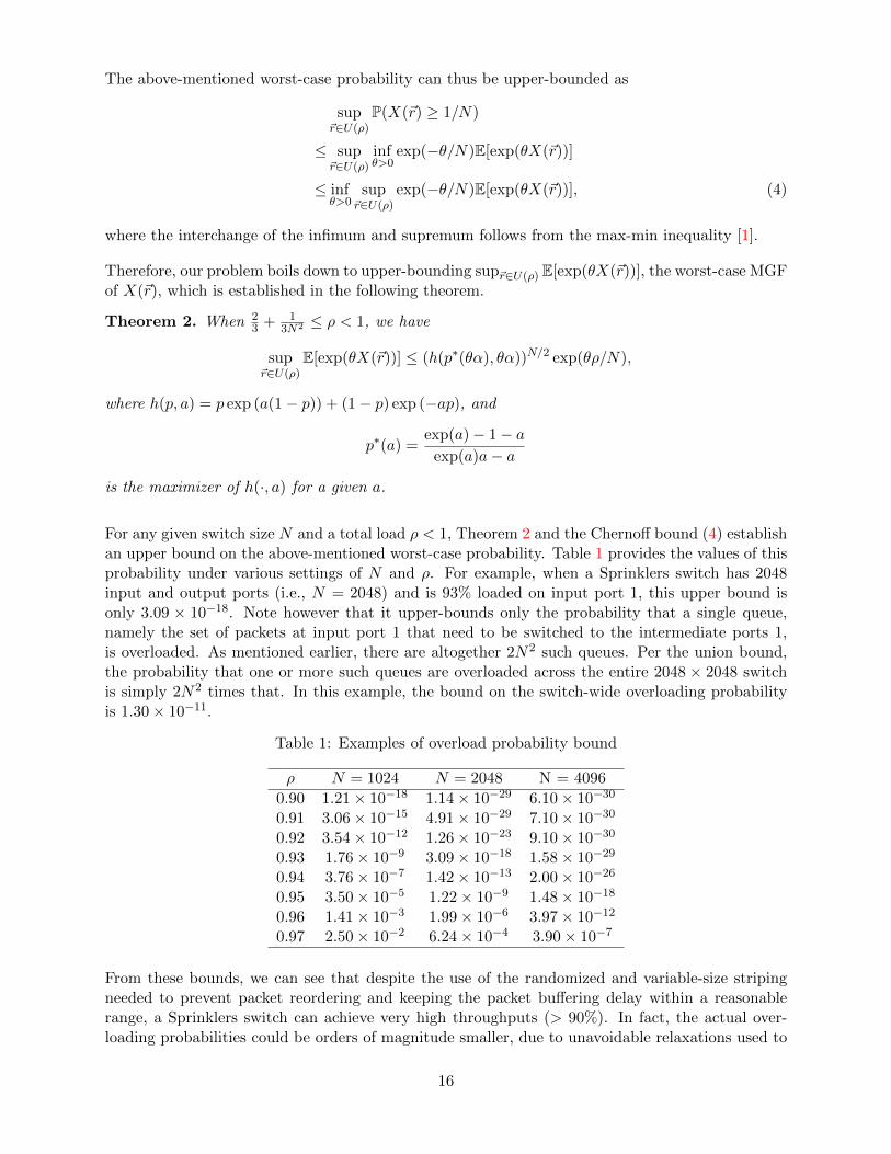
For any given switch size N and a total load ρ < 1, Theorem 2 and the Chernoff bound (4) establishan upper bound on the above-mentioned worst-case probability. Table 1 provides the values of thisprobability under various settings of N and ρ. For example, when a Sprinklers switch has 2048input and output ports (i.e., N = 2048) and is 93% loaded on input port 1, this upper bound isonly 3.09 × 10−18. Note however that it upper-bounds only the probability that a single queue,namely the set of packets at input port 1 that need to be switched to the intermediate ports 1,is overloaded. As mentioned earlier, there are altogether 2N2 such queues. Per the union bound,the probability that one or more such queues are overloaded across the entire 2048 × 2048 switchis simply 2N2 times that. In this example, the bound on the switch-wide overloading probabilityis 1.30× 10−11.

Table 1: Examples of overload probability bound

ρ N = 1024 N = 2048 N = 4096

0.90 1.21× 10−18 1.14× 10−29 6.10× 10−30

0.91 3.06× 10−15 4.91× 10−29 7.10× 10−30

0.92 3.54× 10−12 1.26× 10−23 9.10× 10−30

0.93 1.76× 10−9 3.09× 10−18 1.58× 10−29

0.94 3.76× 10−7 1.42× 10−13 2.00× 10−26

0.95 3.50× 10−5 1.22× 10−9 1.48× 10−18

0.96 1.41× 10−3 1.99× 10−6 3.97× 10−12

0.97 2.50× 10−2 6.24× 10−4 3.90× 10−7

From these bounds, we can see that despite the use of the randomized and variable-size stripingneeded to prevent packet reordering and keeping the packet buffering delay within a reasonablerange, a Sprinklers switch can achieve very high throughputs (> 90%). In fact, the actual over-loading probabilities could be orders of magnitude smaller, due to unavoidable relaxations used to

16

obtain such bounds. Another interesting phenomena reflected in Table 1 is that, given a traffic load,this bound decreases rapidly as the switch size N increases. In other words, the larger a Sprinklersswitch is, the higher the throughput guarantees it can provide. This is certainly a desired propertyfor a scalable switch.

4.2 Proof of Theorem 2

Recall fi = F (ri) and si = rifi

for i = 1, 2, · · · , N . For the convenience of our later derivations, we

rewrite X as a function of ~f and ~s by defining X(~s, ~f) = X(~s◦ ~f), where ~s◦ ~f = (f1 ·s1, f2 ·s2, · · · , fN ·sN ). With this rewriting, we can convert the optimization problem sup~r∈U(ρ) E[exp(θX(~r))] inTheorem 2 to the following:

sup〈~f,~s〉∈A(ρ)

E[exp(θX(~s, ~f))], (5)

where

A(ρ) := {〈~f,~s〉|f` = 2k` for some integer k`, ∀` (6)

s` ∈ [0, α] if f` = 1, (7)

s` ∈ (α/2, α] if f` = 2, 4, · · · , N/2 (8)

s` ∈ (α/2, 1/N ] if f` = N, (9)

N∑`=1

s`f` = ρ}. (10)

The rule for stripe size determination (1) induces the conditions (6) - (9) above.

We now replace the half-open intervals in conditions (8) and (9) by the closed ones, which isequivalent to replacing A(ρ) with its closure A(ρ), because it is generally much easier to work witha closed set in an optimization problem. The resulting optimization problem is

max〈~f,~s〉∈A(ρ)

Eσ[exp(θX(~s, ~f))]. (11)

This replacement is logically correct because it will not decrease the optimal value of this optimiza-tion problem, and we are deriving an upper bound of it.

Our approach to Problem (11) is an exciting combination of convex optimization and the theoryof negative associations in statistics [10], glued together by the Cauchy-Schwartz inequality. Wefirst show that E[exp(θX(~s, ~f))], viewed as a function of only ~s (i.e., with a fixed ~f), achieves itsmaximum over A(ρ) when ~s satisfies certain extremal conditions, through the convex optimizationtheory in Sec. 4.2.1. Then with ~s fixed at any such extreme point, we can decompose X(~s, ~f) intothe sum of two sets of negatively associated (defined below) random variables. Using propertiesof negative association, we are able to derive a very tight upper bound on E[exp(θX(~s, ~f))] inSec. 4.2.2.

Definition 1. Random variables X1, X2, · · · , Xk are said to be negatively associated if for everypair of disjoint subsets A1, A2 of {1, 2, · · · , k},

Cov{g1(Xi, i ∈ A1), g2(Xj , j ∈ A2)} ≤ 0,

whenever g1 and g2 are nondecreasing functions.

17

In the proof below, we need to use the following properties of negative association [10].

Lemma 2. Let g1, g2, · · · , gk be nondecreasing positive functions of one variable. Then X1, · · · , Xk

being negatively associated implies

E

[k∏i=1

gi(Xi)

]≤

k∏i=1

E [gi(Xi)] .

Lemma 3. Let x = (x1, · · · , xk) be a set of k real numbers. X = (X1, · · · , Xk) is a random vector,taking values in the set of k! permutations of x with equal probabilities. Then X = (X1, · · · , Xk) isnegatively associated.

4.2.1 Extremal Property of ~s in An Optimal Solution

Lemma 4. Given 23 + 1

3N2 ≤ ρ < 1, for any θ > 0, there is always an optimal solution 〈~f∗, ~s∗〉 toProblem (11) that satisfies the following property:

s∗j =

{0 or α, if f∗j = 1;α2 or α, if 2 ≤ f∗j ≤ N

2 .(12)

Proof. Suppose 〈~f∗, ~s∗〉 is an optimal solution to Problem (11). We claim that at least one scalarin ~f∗ is equal to N , since otherwise, the total arrival rate is at most 1

N2 · N2 ·N = 12 by the stripe

size determination rule (1), contradicting our assumption that ρ ≥ 23 + 1

3N2 >12 . In addition, if

more than one scalars in ~f∗ are equal to N , we add up the values of all these scalars in ~s, assign thetotal to one of them (say sm), and zero out the rest. This aggregation operation will not changethe total arrival rate to any intermediate port because an input VOQ with stripe size equal to Nwill spread its traffic evenly to all the intermediate ports anyway.

If the optimal solution 〈~f∗, ~s∗〉 does not satisfy Property (12), we show that we can find anotheroptimal solution satisfying Property (12) through the following optimization problem. Note thatnow with ~f∗ fixed, E[exp (θX(~s, ~f∗))] is a function of only ~s.

max~s

: E[exp (θX(~s, ~f∗))] (13)

s.t.:0 ≤ sj ≤ α,∀j with f∗j = 1; (14)α

2≤ sj ≤ α,∀j with 2 ≤ f∗j ≤ N/2; (15)

α/2 ≤ sm; (16)∑j

sjf∗j = ρ. (17)

E[exp (θX(~s, ~f∗))] = 1N !

∑σ exp

(θ∑N

j=1 sj1{f∗j ≥σ(j)}

)where σ(j) is the index of the intermediate

port that VOQ j is mapped to. Given ~f∗, the objective function E[exp (θX(~s, ~f∗))] is clearly aconvex function of ~s.

The feasible region of ~s defined by (14) - (17) is a (convex) polytope. By the convex optimizationtheory [1], the (convex) objective function reaches its optimum at one of the extreme points of

18

the polytope. The assumption ρ ≥ 23 + 1

3N2 implies that Constraint (16) cannot be satisfied withequality. Thus, for any extreme point of the polytope, each of Constraint (14) and (15) mustbe satisfied with equality on one side. Thus there exists at least one optimal solution satisfyingProperty (12). This establishes the required result.

4.2.2 Exploiting Negative Associations

Suppose the optimization objective E[exp (θX(~s, ~f))] is maximized at ~s∗, an extreme point of theabove-mentioned polytope, and ~f∗. In this section, we prove that E[exp (θX(~s∗, ~f∗))] is upper-bounded by the right-hand side (RHS) of the inequality in Theorem 2, by exploiting the negativeassociations – induced by ~s∗ being an extreme point – among the random variables that add up toX(~s∗, ~f∗). For notational convenience, we drop the asterisk from ~s∗ and ~f∗, and simply write themas ~s and ~f .

Again for notational convenience, we further drop the terms ~f and ~s from X(~s, ~f), and simply writeit as X. Such a dependency should be clear from the context. We now split X into two randomvariables XL and XU and a constant Xd, by splitting each s` into sL` and sU` , and each f` intofL` and fU` , as follows. If f` = N , we let sL` = sU` = 0. Otherwise, we define sL` = min{s`, α/2}and sU` = max{0, s` − α/2}. We then define fL` = f`1{sL` =α/2} and fU` = f`1{sU` =α/2}. It is not

hard to verify that sL` + sU` = s` and fL` + fU` = f`, for ∀` if f` ≤ N/2. We further define XL =∑N`=1 α/2 ·1{fL

σ−1(`)≥`} and XU =

∑N`=1 α/2 ·1{fU

σ−1(`)≥`}. Finally, we define Xd =

∑N`=1 s`1{f`=N}.

Xd is the total arrival rate from the (high-rate) VOQs that have stripe size N , which is a constantbecause how much traffic any of these VOQs sends to the queue is not affected by which primaryintermediate port σ maps the VOQ to. It is not hard to verify that X = Xd +XU +XL.

By the Cauchy-Schwartz inequality, we have

E[exp(θX(~r))] = exp(θXd(~r))E[exp(θXU (~r)) exp(θXL(~r))]

≤ exp(θXd(~r))(E[exp(2θXL(~r))]

)1/2·(E[exp(2θXU (~r))]

)1/2. (18)

Let pL` = P(fLσ−1(`) ≥ `). We now upper bound the MGF of XL as follows:

E[exp(2θXL)] = E

[exp

(2θ · α/2 ·

N∑`=1

1{fLσ−1(`)

≥`}

)]

= E

[N∏`=1

exp

(θα1{fL

σ−1(`)≥`}

)]

≤N∏`=1

E[exp

(θα1{fL

σ−1(`)≥`}

)]

=

N/2∏`=1

E[exp

(θα1{fL

σ−1(`)≥`}

)]

≤N/2∏`=1

h(p∗(θα), θα) exp(θαpL` )

19

= (h(p∗(θα), θα))N/2N/2∏`=1

exp(θαpL` ). (19)

The first inequality holds due to Lemma 2 and the following two facts. First, {fLσ−1(1), fLσ−1(2), · · · , f

Lσ−1(N)},

as a uniform random permutation of {fL1 , fL2 , · · · , fLN}, are negatively associated according toLemma 3. Second, exp(θα1{x≥`}) is a nondecreasing function of x for any given ` when θ > 0. The

third equality holds because with the way we define fL above, fLσ−1(`) ≤ N/2 for any `. The last

inequality holds because each term in the product on the left-hand side, E[exp(θα1{fLσ−1(`)

≥`})], is

upper bounded by the corresponding term in the product on the RHS, h(p∗(θα), θα) exp(θαpL` ). Itis not hard to verify because each E[exp(θα1{fL

σ−1(`)≥`})] is the MGF of a Bernoulli random variable

scaled by a constant factor θα, and the function h reaches its maximum at p∗ as defined in Theorem2.

Letting pU` = P(fUσ−1(`) ≥ `), we can similarly bound E[exp(2θXU )] as follows:

E[exp(2θXU )] ≤ (h(p∗(θα), θα))N/2N/2∏`=1

exp(θαpU` ). (20)

Combining (18), (19), and (20), we obtain

E[exp(θX)] ≤(h(p∗(θα), θα))N/2

exp

θ(Xd +α

2

N/2∑`=1

(pL` + pU` ))

= (h(p∗(θα), θα))N/2 exp (θρ/N) .

The final equality holds since ρ/N = E[X] = E[Xd + XL + XU ] = Xd + α2

∑N/2`=1 (pL` + pU` )). This

concludes the proof of the theorem.

5 Expected delay at intermediate stage

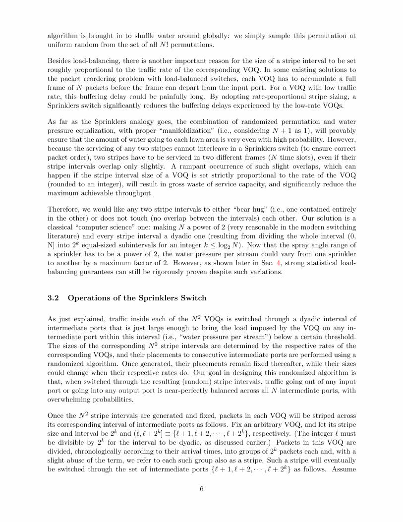
In this section, we analyze the expected queue length at the intermediate ports. We are interestedin this metric for two reasons. First, the queue length at these stations contribute to the total delayof the packets in this switch. Secondly and more importantly, when the switch detects changes ofarrival rates to the input VOQs, the frame sizes of the input VOQs need to be redesigned. Beforethe packets with the new frame sizes are spread to the intermediate ports, the switch needs to makesure that the packets of previous frame sizes are all cleared. Otherwise, there could be reorderingof the packets. The expected duration of this clearance phase is the average queue length at thestations.

We assume that the arrivals in different periods are identical and independently distributed. Fora queuing system, given that the arrival rate is smaller than the service rate, the queue is stableand the queue length is mainly due to the burstiness of the arrivals. To make the arrivals havethe maximum burstiness, we assume the arrival in each cycle (N time slots) is a Bernoulli random

20

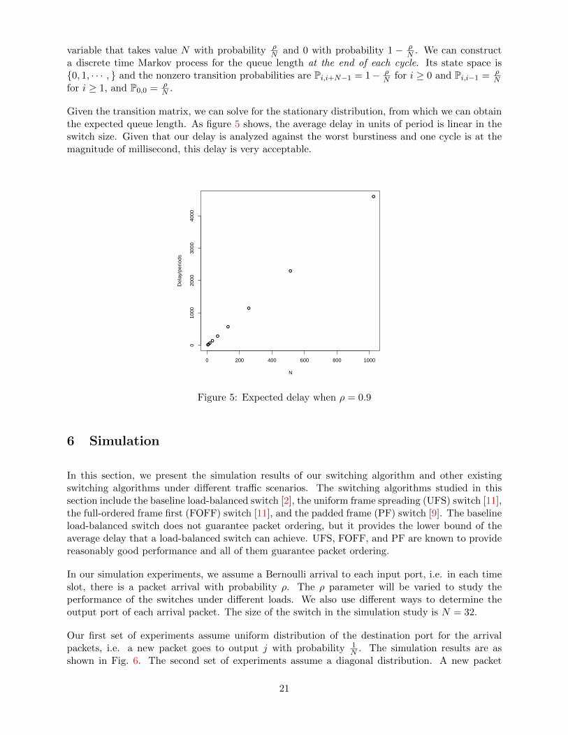
variable that takes value N with probability ρN and 0 with probability 1 − ρ

N . We can constructa discrete time Markov process for the queue length at the end of each cycle. Its state space is{0, 1, · · · , } and the nonzero transition probabilities are Pi,i+N−1 = 1− ρ

N for i ≥ 0 and Pi,i−1 = ρN

for i ≥ 1, and P0,0 = ρN .

Given the transition matrix, we can solve for the stationary distribution, from which we can obtainthe expected queue length. As figure 5 shows, the average delay in units of period is linear in theswitch size. Given that our delay is analyzed against the worst burstiness and one cycle is at themagnitude of millisecond, this delay is very acceptable.

●●●

●

●

●

●

●

●

0 200 400 600 800 1000

010

0020

0030

0040

00

N

Del

ay/p

erio

ds

Figure 5: Expected delay when ρ = 0.9

6 Simulation

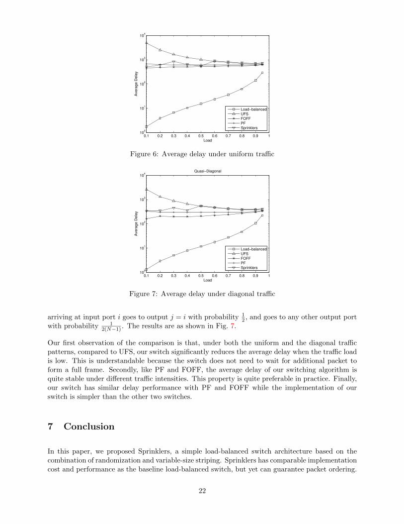
In this section, we present the simulation results of our switching algorithm and other existingswitching algorithms under different traffic scenarios. The switching algorithms studied in thissection include the baseline load-balanced switch [2], the uniform frame spreading (UFS) switch [11],the full-ordered frame first (FOFF) switch [11], and the padded frame (PF) switch [9]. The baselineload-balanced switch does not guarantee packet ordering, but it provides the lower bound of theaverage delay that a load-balanced switch can achieve. UFS, FOFF, and PF are known to providereasonably good performance and all of them guarantee packet ordering.

In our simulation experiments, we assume a Bernoulli arrival to each input port, i.e. in each timeslot, there is a packet arrival with probability ρ. The ρ parameter will be varied to study theperformance of the switches under different loads. We also use different ways to determine theoutput port of each arrival packet. The size of the switch in the simulation study is N = 32.

Our first set of experiments assume uniform distribution of the destination port for the arrivalpackets, i.e. a new packet goes to output j with probability 1

N . The simulation results are asshown in Fig. 6. The second set of experiments assume a diagonal distribution. A new packet

21

0.1 0.2 0.3 0.4 0.5 0.6 0.7 0.8 0.9 110

0

101

102

103

104

Ave

rag

e D

ela

yLoad

Load−balanced

UFS

FOFF

PF

Sprinklers

Figure 6: Average delay under uniform traffic

0.1 0.2 0.3 0.4 0.5 0.6 0.7 0.8 0.9 110

0

101

102

103

104

Ave

rag

e D

ela

y

Load

Quasi−Diagonal

Load−balanced

UFS

FOFF

PF

Sprinklers

Figure 7: Average delay under diagonal traffic

arriving at input port i goes to output j = i with probability 12 , and goes to any other output port

with probability 12(N−1) . The results are as shown in Fig. 7.

Our first observation of the comparison is that, under both the uniform and the diagonal trafficpatterns, compared to UFS, our switch significantly reduces the average delay when the traffic loadis low. This is understandable because the switch does not need to wait for additional packet toform a full frame. Secondly, like PF and FOFF, the average delay of our switching algorithm isquite stable under different traffic intensities. This property is quite preferable in practice. Finally,our switch has similar delay performance with PF and FOFF while the implementation of ourswitch is simpler than the other two switches.

7 Conclusion

In this paper, we proposed Sprinklers, a simple load-balanced switch architecture based on thecombination of randomization and variable-size striping. Sprinklers has comparable implementationcost and performance as the baseline load-balanced switch, but yet can guarantee packet ordering.

22

We rigorously proved using worst-case large deviation techniques that Sprinklers can achieve near-perfect load-balancing under arbitrary admissible traffic. Finally, we believe that this work willserve as a catalyst to a rich family of solutions based on the simple principles of randomization andvariable-size striping.

References

[1] Stephen P Boyd and Lieven Vandenberghe. Convex optimization. Cambridge university press,2004.

[2] Cheng-Shang Chang, Duan-Shin Lee, and Yi-Shean Jou. Load balanced birkhoff–von neumannswitches, part i: one-stage buffering. Computer Communications, 25(6):611–622, 2002.

[3] Cheng-Shang Chang, Duan-Shin Lee, and Ching-Ming Lien. Load balanced birkhoff–von neu-mann switches, part ii: multi-stage buffering. Computer Communications, 25(6):623–634,2002.

[4] Charles J Colbourn. CRC handbook of combinatorial designs. CRC press, 1996.

[5] JG Dai and Balaji Prabhakar. The throughput of data switches with and without speedup. InINFOCOM 2000. Nineteenth Annual Joint Conference of the IEEE Computer and Communi-cations Societies. Proceedings. IEEE, volume 2, pages 556–564. IEEE, 2000.

[6] Andy L Drizen. Generating uniformly distributed random 2-designs with block size 3. Journalof Combinatorial Designs, 20(8):368–380, 2012.

[7] Richard Durstenfeld. Algorithm 235: random permutation. Communications of the ACM, 7(7):420, 1964.

[8] Mark T Jacobson and Peter Matthews. Generating uniformly distributed random latin squares.Journal of Combinatorial Designs, 4(6):405–437, 1996.

[9] Juan Jose Jaramillo, Fabio Milan, and R Srikant. Padded frames: a novel algorithm for stablescheduling in load-balanced switches. Networking, IEEE/ACM Transactions on Networking,16(5):1212–1225, 2008.

[10] Kumar Joag-Dev and Frank Proschan. Negative association of random variables with appli-cations. The Annals of Statistics, 11(1):286–295, 1983.

[11] Isaac Keslassy. The load-balanced router. PhD thesis, Stanford University, 2004.

[12] Leonard Kleinrock. Queueing systems. volume 1: Theory. 1975.

[13] Bill Lin and Isaac Keslassy. The concurrent matching switch architecture. Networking,IEEE/ACM Transactions on, 18(4):1330–1343, 2010.

23