stability and complexity of minimising probabilistic automata
TRANSCRIPT

Stability and Complexity of MinimisingProbabilistic Automata
Stefan Kiefer and Bjorn Wachter
University of Oxford, UK
Abstract. We consider the state-minimisation problem for weightedand probabilistic automata. We provide a numerically stable polynomial-time minimisation algorithm for weighted automata, with guaranteedbounds on the numerical error when run with floating-point arithmetic.Our algorithm can also be used for “lossy” minimisation with boundederror. We show an application in image compression. In the second partof the paper we study the complexity of the minimisation problem forprobabilistic automata. We prove that the problem is NP-hard and inPSPACE, improving a recent EXPTIME-result.
1 Introduction
Probabilistic and weighted automata were introduced in the 1960s, with manyfundamental results established by Schutzenberger [24] and Rabin [22]. Nowa-days probabilistic automata are widely used in automated verification, natural-language processing, and machine learning.
Probabilistic automata (PAs) generalise deterministic finite automata(DFAs): The transition relation specifies, for each state q and each input letter a,a probability distribution on the successor state. Instead of a single initial state,a PA has a probability distribution over states; and instead of accepting states, aPA has an acceptance probability for each state. As a consequence, the languageinduced by a PA is a probabilistic language, i.e., a mapping L : Σ∗ → [0, 1],which assigns each word an acceptance probability. Weighted automata (WAs),in turn, generalise PAs: the numbers appearing in the specification of a WA maybe arbitrary real numbers. As a consequence, a WA induces a weighted language,i.e., a mapping L : Σ∗ → R. Loosely speaking, the weight of a word w is thesum of the weights of all accepting w-labelled paths through the WA.
Given an automaton, it is natural to ask for a small automaton that acceptsthe same weighted language. A small automaton is particularly desirable whenfurther algorithms are run on the automaton, and the runtime of those algo-rithms depends crucially on the size of the automaton [17]. In this paper weconsider the problem of minimising the number of states of a given WA or PA,while preserving its (weighted or probabilistic) language.
WAs can be minimised in polynomial time, using, e.g., the standardisationprocedure of [24]. When implemented efficiently (for instance using triangularmatrices), one obtains an O(|Σ|n3) minimisation algorithm, where n is the num-ber of states. As PAs are special WAs, the same holds in principle for PAs.
arX
iv:1
404.
6673
v2 [
cs.F
L]
1 M
ay 2
014

There are two problems with these algorithms: (1) numerical instability, i.e.,round-off errors can lead to an automaton that is not minimal and/or induces adifferent probabilistic language; and (2) minimising a PA using WA minimisationalgorithms does not necessarily result in a PA: transition weights may, e.g.,become negative. This paper deals with those two issues.
Concerning problem (1), numerical stability is crucial under two scenarios:(a) when the automaton size makes the use of exact rational arithmetic pro-hibitive, and thus necessitates floating-point arithmetic [17]; or (b) when exactminimisation yields an automaton that is still too large and a “lossy compres-sion” is called for, as in image compression [15]. Besides finding a numericallystable algorithm, we aim at two further goals: First, a stable algorithm shouldalso be efficient; i.e., it should be as fast as classical (efficient, but possibly un-stable) algorithms. Second, stability should be provable, and ideally there shouldbe easily computable error bounds. In Section 3 we provide a numerically stableO(|Σ|n3) algorithm for minimising WAs. The algorithm generalises the Arnoldiiteration [2] which is used for locating eigenvalues in numerical linear algebra.The key ingredient, leading to numerical stability and allowing us to give errorbounds, is the use of special orthonormal matrices, called Householder reflec-tors [14]. To the best of the authors’ knowledge, these techniques have not beenpreviously utilised for computations on weighted automata.
Problem (2) suggests a study of the computational complexity of the PA min-imisation problem: given a PA and m ∈ N, is there an equivalent PA with mstates? In the 1960s and 70s, PAs were studied extensively, see the survey [7] forreferences and Paz’s influential textbook [21]. PAs appear in various flavours andunder different names. For instance, in stochastic sequential machines [21] thereis no fixed initial state distribution, so the semantics of a stochastic sequentialmachine is not a probabilistic language, but a mapping from initial distributionsto probabilistic languages. This gives rise to several notions of minimality in thismodel [21]. In this paper we consider only PAs with an initial state distribution;equivalence means equality of probabilistic languages.
One may be tempted to think that PA minimisation is trivially in NP, byguessing the minimal PA and verifying equivalence. However, it is not clear thatthe minimal PA has rational transition probabilities, even if this holds for theoriginal PA.
For DFAs, which are special PAs, an automaton is minimal (i.e., has the leastnumber of states) if and only if all states are reachable and no two states areequivalent. However, this equivalence does in general not hold for PAs. In fact,even if a PA has the property that no state behaves like a convex combination ofother states, the PA may nevertheless not be minimal. As an example, considerthe PA in the middle of Figure 2 on page 9. State 3 behaves like a convexcombination of states 2 and 4: state 3 can be removed by splitting its incomingarc with weight 1 in two arcs with weight 1/2 each and redirecting the new arcsto states 2 and 4. The resulting PA is equivalent and no state can be replacedby a convex combination of other states. But the PA on the right of the figureis equivalent and has even fewer states.
2

In Section 4 we show that the PA minimisation problem is NP-hard by areduction from 3SAT. A step in our reduction is to show that the followingproblem, the hypercube problem, is NP-hard: given a convex polytope P withinthe d-dimensional unit hypercube and m ∈ N, is there a convex polytope withm vertices that is nested between P and the hypercube? We then reduce thehypercube problem to PA minimisation. To the best of the authors’ knowledge,no lower complexity bound for PA minimisation has been previously obtained,and there was no reduction from the hypercube problem to PA minimisation.However, towards the converse direction, the textbook [21] suggests that analgorithm for the hypercube problem could serve as a “subroutine” for a PAminimisation algorithm, leaving the decidability of both problems open. In fact,problems similar to the hypercube problem were subsequently studied in the fieldof computational geometry, citing PA minimisation as a motivation [25,20,11,10].
The PA minimisation problem was shown to be decidable in [19], where theauthors provided an exponential reduction to the existential theory of the reals,which, in turn, is decidable in PSPACE [8,23], but not known to be PSPACE-hard. In Section 4.2 we give a polynomial-time reduction from the PA min-imisation problem to the existential theory of the reals. It follows that the PAminimisation problem is in PSPACE, improving the EXPTIME result of [19].
2 Preliminaries
In the technical development that follows it is more convenient to talk aboutvectors and transition matrices than about states, edges, alphabet labels andweights. However, a PA “of size n” can be easily viewed as a PA with states1, 2, . . . , n. We use this equivalence in pictures.
Let N = {0, 1, 2, . . .}. For n ∈ N we write Nn for the set {1, 2, . . . , n}. Form,n ∈ N, elements of Rm and Rm×n are viewed as vectors and matrices, re-spectively. Vectors are row vectors by default. Let α ∈ Rm and M ∈ Rm×n.We denote the entries by α[i] and M [i, j] for i ∈ Nm and j ∈ Nn. By M [i, ·]we refer to the ith row of M . By α[i..j] for i ≤ j we refer to the sub-vector(α[i], α[i+ 1], . . . , α[j]), and similarly for matrices. We denote the transpose byαT (a column vector) and MT ∈ Rn×m. We write In for the n × n identitymatrix. When the dimension is clear from the context, we write e(i) for thevector with e(i)[i] = 1 and e(i)[j] = 0 for j 6= i. A vector α ∈ Rm is stochasticif α[i] ≥ 0 for all i ∈ Nm and
∑mi=1 α[i] ≤ 1. A matrix is stochastic if all its
rows are stochastic. By ‖·‖ = ‖·‖2, we mean the 2-norm for vectors and matricesthroughout the paper unless specified otherwise. If a matrix M is stochastic,then ‖M‖ ≤ ‖M‖1 ≤ 1. For a set V ⊆ Rn, we write 〈V 〉 to denote the vec-tor space spanned by V , where we often omit the braces when denoting V . Forinstance, if α, β ∈ Rn, then 〈{α, β}〉 = 〈α, β〉 = {rα+ sβ | r, s ∈ R}.
An R-weighted automaton (WA) A = (n,Σ,M,α, η) consists of a sizen ∈ N, a finite alphabet Σ, a map M : Σ → Rn×n, an initial (row) vectorα ∈ Rn, and a final (column) vector η ∈ Rn. Extend M to Σ∗ by settingM(a1 · · · ak) := M(a1) · · ·M(ak). The language LA of a WA A is the mapping
3

LA : Σ∗ → R with LA(w) = αM(w)η. WAs A,B over the same alphabet Σ aresaid to be equivalent if LA = LB. A WA A is minimal if there is no equivalentWA B of smaller size.
A probabilistic automaton (PA) A = (n,Σ,M,α, η) is a WA, where α isstochastic, M(a) is stochastic for all a ∈ Σ, and η ∈ [0, 1]n. A PA is a DFA if allnumbers in M,α, η are 0 or 1.
3 Stable WA Minimisation
In this section we discuss WA minimisation. In Section 3.1 we describe a WAminimisation algorithm in terms of elementary linear algebra. The presentationreminds of Brzozowski’s algorithm for NFA minimisation [6].1 WA minimisationtechniques are well known, originating in [24], cf. also [4, Chapter II] and [3]. Ouralgorithm and its correctness proof may be of independent interest, as they ap-pear to be particularly succinct. In Sections 3.2 and 3.3 we take further advantageof the linear algebra setting and develop a numerically stable WA minimisationalgorithm.
3.1 Brzozowski-like WA Minimisation
Let A = (n,Σ,M,α, η) be a WA. Define the forward space of A as the (row)vector space F := 〈αM(w) | w ∈ Σ∗〉. Similarly, let the backward space of A bethe (column) vector space B := 〈M(w)η | w ∈ Σ∗〉. Let −→n ∈ N and F ∈ R−→n×nsuch that the rows of F form a basis of F. Similarly, let ←−n ∈ N and B ∈ Rn×←−nsuch that the columns of B form a basis of B. Since FM(a) ⊆ F and M(a)B ⊆ B
for all a ∈ Σ, there exist maps−→M : Σ → R−→n×−→n and
←−M : Σ → R←−n×←−n such that
FM(a) =−→M(a)F and M(a)B = B
←−M(a) for all a ∈ Σ. (1)
We call (F,−→M) a forward reduction and (B,
←−M) a backward reduction. We will
show that minimisation reduces to computing such reductions. By symmetry we
can focus on forward reductions. We call a forward reduction (F,−→M) canonical
if F [1, ·] (i.e., the first row of F ) is a multiple of α, and the rows of F areorthonormal, i.e., FFT = I−→n .
Let A = (n,Σ,M,α, η) be a WA with forward and backward reductions
(F,−→M) and (B,
←−M), respectively. Let −→α ∈ R−→n be a row vector such that
α = −→αF ; let ←−η ∈ R←−n be a column vector such that η = B←−η . (If (F,−→M) is
canonical, we have −→α = (±‖α‖, 0, . . . , 0).) Call−→A := (−→n ,Σ,
−→M,−→α , Fη) a for-
ward WA of A with base F and←−A := (←−n ,Σ,
←−M,αB,←−η ) a backward WA of A
with base B. By extending (1) one can see that these automata are equivalentto A:
1 In [5] a very general Brzozowski-like minimization algorithm is presented in termsof universal algebra. One can show that it specialises to ours in the WA setting.
4

Proposition 1. Let A be a WA. Then LA = L−→A = L←−A .
Further, applying both constructions consecutively yields a minimal WA:
Theorem 2. Let A be a WA. Let A′ =←−−→A or A′ =
−→←−A . Then A′ is minimal and
equivalent to A.
Theorem 2 mirrors Brzozowski’s NFA minimisation algorithm. We give a shortproof in Appendix A.2.
3.2 Numerically Stable WA Minimisation
Theorem 2 reduces the problem of minimising a WA to the problem of comput-ing a forward and a backward reduction. In the following we focus on computing
a canonical (see above for the definition) forward reduction (F,−→M). Figure 1
shows a generalisation of Arnoldi’s iteration [2] to multiple matrices. Arnoldi’siteration is typically used for locating eigenvalues [12]. Its generalisation to mul-tiple matrices is novel, to the best of the authors’s knowledge. Using (1) one cansee that it computes a canonical forward reduction by iteratively extending apartial orthonormal basis {f1, . . . , fj} for the forward space F.
function ArnoldiReductioninput: α ∈ Rn; M : Σ → Rn×n
output: canonical forward reduction (F,−→M) with F ∈ R
−→n×n and−→M : Σ → R
−→n×−→n
` := 0; j := 1; f1 := α/‖α‖ (or f1 := −α/‖α‖)while ` < j do
` := `+ 1for a ∈ Σ do
if f`M(a) 6∈ 〈f1, . . . , fj〉j := j + 1define fj orthonormal to f1, . . . , fj−1 such that
〈f1, . . . , fj−1, f`M(a)〉 = 〈f1, . . . , fj〉define
−→M(a)[`, ·] such that f`M(a) =
∑ji=1
−→M(a)[`, i]fi
and−→M(a)[`, j+1..n] = (0, . . . , 0)
−→n := j; form F ∈ R−→n×−→n with rows f1, . . . , f−→n
return F and−→M(a)[1..−→n , 1..−→n ] for all a ∈ Σ
Fig. 1: Generalised Arnoldi iteration.
For efficiency, one would like to run generalised Arnoldi iteration (Figure 1)using floating-point arithmetic. This leads to round-off errors. The check “iff`M(a) 6∈ 〈f1, . . . , fj〉” is particularly problematic: since the vectors f1, . . . , fjare computed with floating-point arithmetic, we cannot expect that f`M(a) liesexactly in the vector space spanned by those vectors, even if that would bethe case without round-off errors. As a consequence, we need to introduce anerror tolerance parameter τ > 0, so that the check “f`M(a) 6∈ 〈f1, . . . , fj〉”returns true only if f`M(a) has a “distance” of more than τ to the vector space
5
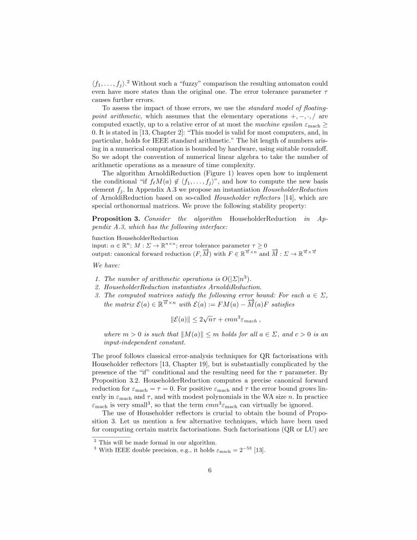
〈f1, . . . , fj〉.2 Without such a “fuzzy” comparison the resulting automaton couldeven have more states than the original one. The error tolerance parameter τcauses further errors.
To assess the impact of those errors, we use the standard model of floating-point arithmetic, which assumes that the elementary operations +,−, ·, / arecomputed exactly, up to a relative error of at most the machine epsilon εmach ≥0. It is stated in [13, Chapter 2]: “This model is valid for most computers, and, inparticular, holds for IEEE standard arithmetic.” The bit length of numbers aris-ing in a numerical computation is bounded by hardware, using suitable roundoff.So we adopt the convention of numerical linear algebra to take the number ofarithmetic operations as a measure of time complexity.
The algorithm ArnoldiReduction (Figure 1) leaves open how to implementthe conditional “if f`M(a) 6∈ 〈f1, . . . , fj〉”, and how to compute the new basiselement fj . In Appendix A.3 we propose an instantiation HouseholderReductionof ArnoldiReduction based on so-called Householder reflectors [14], which arespecial orthonormal matrices. We prove the following stability property:
Proposition 3. Consider the algorithm HouseholderReduction in Ap-pendix A.3, which has the following interface:
function HouseholderReductioninput: α ∈ Rn; M : Σ → Rn×n; error tolerance parameter τ ≥ 0
output: canonical forward reduction (F,−→M) with F ∈ R
−→n×n and−→M : Σ → R
−→n×−→n
We have:
1. The number of arithmetic operations is O(|Σ|n3).2. HouseholderReduction instantiates ArnoldiReduction.3. The computed matrices satisfy the following error bound: For each a ∈ Σ,
the matrix E(a) ∈ R−→n×n with E(a) := FM(a)−−→M(a)F satisfies
‖E(a)‖ ≤ 2√nτ + cmn3εmach ,
where m > 0 is such that ‖M(a)‖ ≤ m holds for all a ∈ Σ, and c > 0 is aninput-independent constant.
The proof follows classical error-analysis techniques for QR factorisations withHouseholder reflectors [13, Chapter 19], but is substantially complicated by thepresence of the “if” conditional and the resulting need for the τ parameter. ByProposition 3.2. HouseholderReduction computes a precise canonical forwardreduction for εmach = τ = 0. For positive εmach and τ the error bound grows lin-early in εmach and τ , and with modest polynomials in the WA size n. In practiceεmach is very small3, so that the term cmn3εmach can virtually be ignored.
The use of Householder reflectors is crucial to obtain the bound of Propo-sition 3. Let us mention a few alternative techniques, which have been usedfor computing certain matrix factorisations. Such factorisations (QR or LU) are
2 This will be made formal in our algorithm.3 With IEEE double precision, e.g., it holds εmach = 2−53 [13].
6

related to our algorithm. Gaussian elimination can also be used for WA min-imisation in time O(|Σ|n3), but its stability is governed by the growth factor,which can be exponential even with pivoting [13, Chapter 9], so the bound on‖E(a)‖ in Proposition 3 would include a term of the form 2nεmach. The moststraightforward implementation of ArnoldiReduction would use the ClassicalGram-Schmidt process, which is highly unstable [13, Chapter 19.8]. A variant,the Modified Gram-Schmidt process is stable, but the error analysis is compli-cated by a possibly loss of orthogonality of the computed matrix F . The extentof that loss depends on certain condition numbers (cf. [13, Equation (19.30)]),which are hard to estimate or control in our case. In contrast, our error boundis independent of condition numbers.
Using Theorem 2 we can prove:
Theorem 4. Consider the following algorithm:
function HouseholderMinimisationinput: WA A = (n,Σ,M,α, η); error tolerance parameter τ ≥ 0output: minimised WA A′ = (n′, Σ,M ′, α′, η′).
compute forward reduction (F,−→M) of A using HouseholderReduction
form−→A := (−→n ,Σ,
−→M,−→α ,−→η ) as the forward WA of A with base F
compute backward reduction (B,M ′) of−→A using HouseholderReduction
form A′ := (n′, Σ,M ′, α′, η′) as the backward WA of−→A with base B
return A′
We have:
1. The number of arithmetic operations is O(|Σ|n3).2. For εmach = τ = 0, the computed WA A′ is minimal and equivalent to A.3. Let τ > 0. Let m > 0 such that ‖A‖ ≤ m holds for all
A ∈ {M(a),−→M(a),M ′(a) | a ∈ Σ}. Then for all w ∈ Σ∗ we have
|LA(w)− LA′(w)| ≤ 4|w|‖α‖m|w|−1‖η‖√nτ
+ cmax{|w|, 1}‖α‖m|w|‖η‖n3εmach ,
where c > 0 is an input-independent constant.
The algorithm computes a backward reduction by running the straightforwardbackward variant of HouseholderReduction. We remark that for PAs one cantake m = 1 for the norm bound m from part 3. of the theorem (or m = 1 + ε fora small ε if unfortunate roundoff errors occur). It is hard to avoid an error boundexponential in the word length |w|, as |LA(w)| itself may be exponential in |w|(consider a WA of size 1 with M(a) = 2). Theorem 4 is proved in Appendix A.5.
The error bounds in Proposition 3 and Theorem 4 suggest to choose a smallvalue for the error tolerance parameter τ . But as we have discussed, the computedWA may be non-minimal if τ is set too small or even to 0, intuitively becauseround-off errors may cause the algorithm to overlook minimisation opportunities.So it seems advisable to choose τ smaller (by a few orders of magnitude) than thedesired bound on ‖E(a)‖, but larger (by a few orders of magnitude) than εmach.
7

Note that for εmach > 0 Theorem 4 does not provide a bound on the number ofstates of A′.
To illustrate the stability issue we have experimented with minimising a PAAderived from Herman’s protocol as in [17]. The PA has 190 states and Σ = {a}.When minimising with the (unstable) Classical Gram-Schmidt process, we havemeasured a huge error of |LA(a190) − LA′(a
190)| ≈ 1036. With the ModifiedGram-Schmidt process and the method from Theorem 4 the corresponding errorswere about 10−7, which is in the same order as the error tolerance parameter τ .
3.3 Lossy WA Minimisation
A larger error tolerance parameter τ leads to more “aggressive” minimisationof a possibly already minimal WA. The price to pay is a shift in the language:one would expect only L′A(w) ≈ LA(w). Theorem 4 provides a bound on thisimprecision. In this section we illustrate the trade-off between size and precisionusing an application in image compression.
Weighted automata can be used for image compression, as suggested by Cu-lik et al. [15]. An image, represented as a two-dimensional matrix of grey-scalevalues, can be encoded as a weighted automaton where each pixel is addressedby a unique word. To obtain this automaton, the image is recursively subdividedinto quadrants. There is a state for each quadrant and transitions from a quad-rant to its sub-quadrants. At the level of the pixels, the automaton accepts withthe correct grey-scale value.
Following this idea, we have implemented a prototype tool for image com-pression based on the algorithm of Theorem 4. We give details and show examplepictures in Appendix A.6. This application illustrates lossy minimisation. Thepoint is that Theorem 4 guarantees bounds on the loss.
4 The Complexity of PA Minimisation
Given a PA A = (n,Σ,M,α, η) and n′ ∈ N, the PA minimisation problemasks whether there exists a PA A′ = (n′, Σ,M ′, α′, η′) so that A and A′ areequivalent. For the complexity results in this section we assume that the numbersin the description of the given PA are fractions of natural numbers representedin binary, so they are rational. In Section 4.1 we show that the minimisationproblem is NP-hard. In Section 4.2 we show that the problem is in PSPACE byproviding a polynomial-time reduction to the existential theory of the reals.
4.1 NP-Hardness
We will show:
Theorem 5. The PA minimisation problem is NP-hard.
8

For the proof we reduce from a geometrical problem, the hypercube problem,which we show to be NP-hard. Given d ∈ N, a finite set P = {p1, . . . , pk} ⊆ [0, 1]d
of vectors (“points”) within the d-dimensional unit hypercube, and ` ∈ N, thehypercube problem asks whether there is a set Q = {q1, . . . , q`} ⊆ [0, 1]d of atmost ` points within the hypercube such that conv(Q) ⊇ P , where
conv(Q) := {λ1q1 + · · ·+ λ`q` | λ1, . . . , λ` ≥ 0, λ1 + · · ·+ λ` = 1}
denotes the convex hull of Q. Geometrically, the convex hull of P can be viewedas a convex polytope, nested inside the hypercube, which is another convexpolytope. The hypercube problem asks whether a convex polytope with at most` vertices can be nested in between those polytopes. The answer is trivially yes,if ` ≥ k (take Q = P ) or if ` ≥ 2d (take Q = {0, 1}d). We speak of the restrictedhypercube problem if P contains the origin (0, . . . , 0). We prove the following:
Proposition 6. The restricted hypercube problem can in polynomial time bereduced to the PA minimisation problem.
Proof (sketch). Let d ∈ N and P = {p1, . . . , pk} ⊆ [0, 1]d and ` ∈ N be aninstance of the restricted hypercube problem, where p1 = (0, . . . , 0) and ` ≥ 1.We construct in polynomial time a PA A = (k + 1, Σ,M,α, η) such that thereis a set Q = {q1, . . . , q`} ⊆ [0, 1]d with conv(Q) ⊇ P if and only if there is a PAA′ = (`+ 1, Σ,M ′, α′, η′) equivalent to A. Take Σ := {a2, . . . , ak}∪{b1, . . . , bd}.Set M(ai)[1, i] := 1 and M(bs)[i, k + 1] := pi[s] for all i ∈ {2, . . . , k} and alls ∈ Nd, and set all other entries of M to 0. Set α := e(1) and η := e(k + 1)T .Figure 2 shows an example of this reduction. We prove the correctness of thisreduction in Appendix B.1. ut
p1
p2
p3
p4
p5
1
2
3
4
5
6
1a2 34b2
1a314b1 1
2b2
1a4 12b1
14b2
1a512b1
34b2
1
2
3
4
34a2
38a3
12a5
1b2
14a3
12a4
12a5
1b1
12b2
Fig. 2: Reduction from the hypercube problem to the minimisation problem.The left figure shows an instance of the hypercube problem with d = 2 andP = {p1, . . . , p5} = {(0, 0), (0, 34 ), ( 1
4 ,12 ), ( 1
2 ,14 ), ( 1
2 ,34 )}. It also suggests a set
Q = {(0, 0), (0, 1), (1, 12 )} with conv(Q) ⊇ P . The middle figure depicts thePA A obtained from P . The right figure depicts a minimal equivalent PA A′,corresponding to the set Q suggested in the left figure.
9

Next we show that the hypercube problem is NP-hard, which together withProposition 6 implies Theorem 5. A related problem is known4 to be NP-hard:
Theorem 7 (Theorem 4.2 of [10]). Given two nested convex polyhedra inthree dimensions, the problem of nesting a convex polyhedron with minimumfaces between the two polyhedra is NP-hard.
Note that this NP-hardness result holds even in d = 3 dimensions. However,the outer polyhedron is not required to be a cube, and the problem is aboutminimising the number of faces rather than the number of vertices. Using acompletely different technique we show:
Proposition 8. The hypercube problem is NP-hard. This holds even for therestricted hypercube problem.
The proof is by a reduction from 3SAT, see Appendix B.2.
Remark 9. The hypercube problem is in PSPACE, by appealing to decision al-gorithms for ExTh(R), the existential fragment of the first-order theory of thereals. For every fixed d the hypercube problem is5 in P , exploiting the fact thatExTh(R) can be decided in polynomial time, if the number of variables is fixed.(For d = 2 an efficient algorithm is provided in [1].) It is an open questionwhether the hypercube problem is in NP. It is also open whether the search fora minimum Q can be restricted to sets of points with rational coordinates (thisholds for d = 2).
Propositions 6 and 8 together imply Theorem 5.
4.2 Reduction to the Existential Theory of the Reals
In this section we reduce the PA minimisation problem to ExTh(R), the existen-tial fragment of the first-order theory of the reals. A formula of ExTh(R) is of theform ∃x1 . . . ∃xmR(x1, . . . , xn), where R(x1, . . . , xn) is a boolean combination ofcomparisons of the form p(x1, . . . , xn) ∼ 0, where p(x1, . . . , xn) is a multivariatepolynomial and ∼ ∈ {<,>,≤,≥,=, 6=}. The validity of closed formulas (m = n)is decidable in PSPACE [8,23], and is not known to be PSPACE-hard.
Proposition 10. Let A1 = (n1, Σ,M1, α1, η1) be a PA. A PAA2 = (n2, Σ,M2, α2, η2) is equivalent to A1 if and only if there exist ma-
trices−→M(a) ∈ R(n1+n2)×(n1+n2) for a ∈ Σ and a matrix F ∈ R(n1+n2)×(n1+n2)
such that F [1, ·] = (α1, α2), and F (ηT1 ,−ηT2 )T = (0, . . . , 0)T , and
F
(M1(a) 0
0 M2(a)
)=−→M(a)F for all a ∈ Σ.
The proof is in Appendix B.3. The conditions of Proposition 10 on A2, includingthat it be a PA, can be phrased in ExTh(R). Thus it follows:
4 The authors thank Joseph O’Rourke for pointing out [10].5 This observation is in part due to Radu Grigore.
10

Theorem 11. The PA minimisation problem can be reduced in polynomial timeto ExTh(R). Hence, PA minimisation is in PSPACE.
Theorem 11 improves on a result in [19] where the minimisation problemwas shown to be in EXPTIME. (More precisely, Theorem 4 of [19] states thata minimal PA can be computed in EXPSPACE, but the proof reveals that thedecision problem can be solved in EXPTIME.)
5 Conclusions and Open Questions
We have developed a numerically stable and efficient algorithm for minimisingWAs, based on linear algebra and Brzozowski-like automata minimisation. Wehave given bounds on the minimisation error in terms of both the machine epsilonand the error tolerance parameter τ .
We have shown NP-hardness for PA minimisation, and have given apolynomial-time reduction to ExTh(R). Our work leaves open the precise com-plexity of the PA minimisation problem. The authors do not know whether thesearch for a minimal PA can be restricted to PAs with rational numbers. Asstated in the Remark after Proposition 8, the corresponding question is openeven for the hypercube problem. If rational numbers indeed suffice, then an NPalgorithm might exist that guesses the (rational numbers of the) minimal PAand checks for equivalence with the given PA. Proving PSPACE-hardness wouldimply PSPACE-hardness of ExTh(R), thus solving a longstanding open problem.
For comparison, the corresponding minimisation problems involving WAs (ageneralisation of PAs) and DFAs (a special case of PAs) lie in P . More precisely,minimisation of WAs (with rational numbers) is in randomised NC [18], and DFAminimisation is NL-complete [9]. NFA minimisation is PSPACE-complete [16].
Acknowledgements. The authors would like to thank James Worrell, RaduGrigore, and Joseph O’Rourke for valuable discussions, and the anonymous ref-erees for their helpful comments. Stefan Kiefer is supported by a Royal SocietyUniversity Research Fellowship.
References
1. A. Aggarwal, H. Booth, J. O’Rourke, S. Suri, and C. K. Yap. Finding minimalconvex nested polygons. Information and Computation, 83(1):98–110, 1989.
2. W.E. Arnoldi. The principle of minimized iteration in the solution of the matrixeigenvalue problem. Quarterly of Applied Mathematics, 9:17–29, 1951.
3. A. Beimel, F. Bergadano, N.H. Bshouty, E. Kushilevitz, and S. Varricchio. Learningfunctions represented as multiplicity automata. Journal of the ACM, 47(3):506–530, 2000.
4. J. Berstel and C. Reutenauer. Rational Series and Their Languages. Springer,1988.
5. F. Bonchi, M.M. Bonsangue, H.H. Hansen, P. Panangaden, J.J.M.M. Rutten, andA. Silva. Algebra-coalgebra duality in Brzozowski’s minimization algorithm. ACMTransactions on Computational Logic, to appear.
11

6. J.A. Brzozowski. Canonical regular expressions and minimal state graphs for def-inite events. In Symposium on Mathematical Theory of Automata, volume 12 ofMRI Symposia Series, pages 529–561. Polytechnic Press, Polytechnic Institute ofBrooklyn, 1962.
7. R.G. Bukharaev. Probabilistic automata. Journal of Soviet Mathematics,13(3):359–386, 1980.
8. J. Canny. Some algebraic and geometric computations in PSPACE. In Proceedingsof STOC’88, pages 460–467, 1988.
9. S. Cho and D.T. Huynh. The parallel complexity of finite-state automata problems.Information and Computation, 97(1):1–22, 1992.
10. G. Das and M.T. Goodrich. On the complexity of approximating and illuminatingthree-dimensional convex polyhedra. In Proceedings of Workshop on Algorithmsand Data Structures, volume 955 of LNCS, pages 74–85. Springer, 1995.
11. G. Das and D. Joseph. Minimum vertex hulls for polyhedral domains. TheoreticalComputer Science, 103(1):107–135, 1992.
12. G.H. Golub and C.F. van Loan. Matrix Computations. John Hopkins UniversityPress, 1989.
13. N.J. Higham. Accuracy and Stability of Numerical Algorithms. SIAM, secondedition, 2002.
14. A.S. Householder. Unitary triangularization of a nonsymmetric matrix. Journalof the ACM, 5(4):339–342, 1958.
15. K. Culik II and J. Kari. Image compression using weighted finite automata. Com-puters & Graphics, 17(3):305–313, 1993.
16. T. Jiang and B. Ravikumar. Minimal NFA problems are hard. SIAM Journal onComputing, 22(6):1117–1141, 1993.
17. S. Kiefer, A.S. Murawski, J. Ouaknine, B. Wachter, and J. Worrell. Languageequivalence for probabilistic automata. In Proceedings of CAV, volume 6806 ofLNCS, pages 526–540, 2011.
18. S. Kiefer, A.S. Murawski, J. Ouaknine, B. Wachter, and J. Worrell. On the com-plexity of equivalence and minimisation for Q-weighted automata. Logical Methodsin Computer Science, 9(1:8):1–22, 2013.
19. P. Mateus, D. Qiu, and L. Li. On the complexity of minimizing probabilistic andquantum automata. Information and Computation, 218:36–53, 2012.
20. J.S.B. Mitchell and S. Suri. Separation and approximation of polyhedral objects.In Proceedings of SODA, pages 296–306, 1992.
21. A. Paz. Introduction to probabilistic automata. Academic Press, 1971.22. M.O. Rabin. Probabilistic automata. Information and Control, 6 (3):230–245,
1963.23. J. Renegar. On the computational complexity and geometry of the first-order
theory of the reals. Parts I–III. Journal of Symbolic Computation, 13(3):255–352,1992.
24. M.-P. Schutzenberger. On the definition of a family of automata. Information andControl, 4:245–270, 1961.
25. C.B. Silio. An efficient simplex coverability algorithm in E2 with application tostochastic sequential machines. IEEE Transactions on Computers, C-28(2):109–120, 1979.
26. W. Tzeng. A polynomial-time algorithm for the equivalence of probabilistic au-tomata. SIAM Journal on Computing, 21(2):216–227, 1992.
12

A Proofs of Section 3
A.1 Proof of Proposition 1
Proposition 1. Let A be a WA. Then LA = L−→A = L←−A .
Proof. Observe that the equalities (1) extend inductively to words:
FM(w) =−→M(w)F and M(w)B = B
←−M(w) for all w ∈ Σ∗. (2)
Using (2) and the definition of −→α we have for all w ∈ Σ∗:
LA(w) = αM(w)η = −→αFM(w)η = −→α−→M(w)Fη = L−→A (w) .
Symmetrically one can show LA = L←−A . ut
A.2 Proof of Theorem 2
We will use the notion of a Hankel matrix [4,3]:
Definition 12. Let L : Σ∗ → R. The Hankel matrix of L is the matrixHL ∈ RΣ∗×Σ∗ with HL[x, y] = L(xy) for all x, y ∈ Σ∗. We define rank(L) :=rank(HL).
We have the following proposition:
Proposition 13. Let A be an automaton of size n. Then rank(LA) ≤ n.
Proof. Consider the matrices F : RΣ∗×n and B : Rn×Σ∗ with F [w, ·] := αM(w)
and B[·, w] := M(w)η for all w ∈ Σ∗. Note that rank(F ) ≤ n and rank(B) ≤ n.
Let x, y ∈ Σ∗. Then (F B)[x, y] = αM(x)M(y)η = LA(xy), so F B is the Hankel
matrix of LA. Hence rank(LA) = rank(F B) ≤ min{rank(F ), rank(B)} ≤ n. ut
Now we can prove the theorem:
Theorem 2. Let A be a WA. Let A′ =←−−→A or A′ =
−→←−A . Then A′ is minimal
and equivalent to A.
Proof. W.l.o.g. we assume A′ =−→←−A . Let A = (n,Σ,M,α, η). Let
←−A =
(←−n ,Σ,←−M,αB,←−η ) be a backward automaton of A with base B. Let
−→←−A be a
forward automaton of←−A with base F . Equivalence of A,
←−A and
−→←−A follows from
Proposition 1. Assume that−→←−A has
−→←−n states. For minimality, by Proposition 13,
13

it suffices to show−→←−n = rank(H), where H is the Hankel matrix of LA. Let F
and B be the matrices from the proof of Proposition 13. We have:
−→←−n = rank(F ) (definition of−→←−n )
= dim〈αB←−M(w) | w ∈ Σ∗〉 (definition of F )
= dim〈αM(w)B | w ∈ Σ∗〉 (by (2))
= rank(FB) (definition of F )
= dim〈FM(w)η | w ∈ Σ∗〉 (definition of B)
= rank(F B) (definition of B)
= rank(H) (proof of Proposition 13) .
ut
A.3 Instantiation of ArnoldiReduction with Householder Reflectors
Fix n ≥ 1. For a row vector x ∈ Rk with k ∈ Nn and ‖x‖ 6= 0, the Householderreflector P for x is defined as the matrix
P =
(In−k 0
0 R
)∈ Rn×n ,
where R = Ik − 2vT v ∈ Rk×k, and
v =(x[1] + sign(x[1])‖x‖, x[2], . . . , x[k])
‖(x[1] + sign(x[1])‖x‖, x[2], . . . , x[k])‖∈ Rk ,
where sign(r) = +1 if r ≥ 0 and −1 otherwise. (The careful choice of the signhere is to ensure numerical stability.) To understand this definition better, firstobserve that v is a row vector with ‖v‖ = 1. It is easy to verify that R andthus P are orthonormal and symmetric. Moreover, we have RR = Ik and thusPP = In, i.e., P = PT = P−1. Geometrically, R describes a reflection aboutthe hyperplane through the origin and orthogonal to v ∈ Rk [13, Chapter 19.1].Crucially, the vector v is designed so that R reflects x onto the first axis, i.e.,xR = (±‖x‖, 0, . . . , 0).
Figure 3 shows an instantiation of the algorithm from Figure 1 using House-holder reflectors. Below we prove correctness by showing that Householder-Reduction indeed refines ArnoldiReduction, assuming τ = 0 for the error toler-ance parameter. For efficiency it is important not to form the reflectors P1, P2, . . .explicitly. If P is the Householder reflector for x ∈ Rk, it suffices to keepthe vector v ∈ Rk from the definition of Householder reflectors. A multipli-cation y := yP (for a row vector y ∈ Rn) can then be implemented in O(n)with y[(n−k+1)..n] := y[(n−k+1)..n] − 2
(y[(n−k+1)..n] · vT
)v. This gives an
O(|Σ|n3) number of arithmetic operations of HouseholderReduction.
14

function HouseholderReductioninput: α ∈ Rn; M : Σ → Rn×n; error tolerance parameter τ ≥ 0
output: canonical forward reduction (F,−→M) with F ∈ R
−→n×n and−→M : Σ → R
−→n×−→n
P1 := Householder reflector for α/‖α‖` := 0; j := 1; f1 := e(1)P1
while ` < j do` := `+ 1for a ∈ Σ do−→
M(a)[`, ·] := f`M(a)P1 · · ·Pj
if j + 1 ≤ n and ‖−→M(a)[`, j+1..n]‖ > τ
j := j + 1
Pj := Householder reflector for−→M(a)[`, j..n]
−→M(a)[`, ·] :=
−→M(a)[`, ·]Pj
fj := e(j)Pj · · ·P1−→n := j; form F ∈ R−→n×n with rows f1, . . . , f−→n
return F and−→M(a)[1..−→n , 1..−→n ] for all a ∈ Σ
Fig. 3: Instantiation of ArnoldiReduction (Fig. 1) using Householder reflectors.
HouseholderReduction Instantiates ArnoldiReduction. LetP1, . . . , P−→n ∈ Rn×n be the reflectors computed in HouseholderReduction.Recall that we have PTj = P−1j = Pj . For 0 ≤ j ≤ −→n define
Fj := PjPj−1 · · ·P1 .
The matrices Fj ∈ Rn×n are orthonormal. Since for all j < −→n the reflector Pj+1
leaves the first j rows of Fj unchanged, the first j rows of Fj , . . . , F−→n coincidewith the vectors f1, . . . , fj computed in HouseholderReduction.
First we consider the initialisation part before the while loop. Since P1 is theHouseholder reflector for α/‖α‖, we have (α/‖α‖)P1 = (±1, 0, . . . , 0). It followsthat we have f1 = e(1)P1 = ±α/‖α‖, as in ArnoldiReduction.
Now we consider the while loop. Consider an arbitrary iteration of the
“for a ∈ Σ do” loop. Directly after the loop head we have−→M(a)[`, ·] =
f`M(a)P1 · · ·Pj , hence f`M(a) =−→M(a)[`, ·]Fj . As Fj is orthonormal and its
first j rows coincide with f1, . . . , fj , we have f`M(a) ∈ 〈f1, . . . , fj〉 if and
only if−→M(a)[`, j+1..n] = (0, . . . , 0). This corresponds to the “if” conditional
in ArnoldiReduction. It remains to be shown that−→M(a)[`, ·] is defined as in
ArnoldiReduction:
– Let−→M(a)[`, j+1..n] = (0, . . . , 0). Then at the end of the loop we have
f`M(a) =∑ji=1
−→M(a)[`, i]fi, as required in ArnoldiReduction.
– Let−→M(a)[`, j+1..n] 6= (0, . . . , 0). Then we have:
f`M(a) =−→M(a)[`, ·]Fj (as argued above)
=−→M(a)[`, ·]Pj+1Pj+1Fj (as Pj+1Pj+1 = In)
=−→M(a)[`, ·]Pj+1Fj+1 (by definition of Fj+1)
15

Further, the reflector Pj+1 is designed such that−→M(a)[`, j+1..n] =
(r, 0, . . . , 0) for some r 6= 0. So after increasing j, and updating−→M(a)[`, ·],
and defining the new vector fj , at the end of the loop we have f`M(a) =∑ji=1
−→M(a)[`, i]fi, as required in ArnoldiReduction.
A.4 Proof of Proposition 3
Proposition 3. Consider HouseholderReduction (Figure 3). We have:
1. The number of arithmetic operations is O(|Σ|n3).2. HouseholderReduction instantiates ArnoldiReduction.3. The computed matrices satisfy the following error bound: For each a ∈ Σ,
the matrix E(a) ∈ R−→n×n with E(a) := FM(a)−−→M(a)F satisfies
‖E(a)‖ ≤ 2√nτ + cmn3εmach ,
where m > 0 is such that ‖M(a)‖ ≤ m holds for all a ∈ Σ, and c > 0 is aninput-independent constant.
Proof. The fact that HouseholderReduction is an instance of ArnoldiReductionwas proved in the previous subsection. There we also showed the bound on thenumber of arithmetic operations. It remains to prove the error bound. In orderto highlight the gist of the argument we consider first the case εmach = 0. For0 ≤ j ≤ n we write Fj := PjPj−1 · · ·P1. Recall that f1, . . . , fj , i.e., the first jrows of F , coincide with the first j rows of Fj . We have at the end of the forloop:
f`M(a) =−→M(a)[`, 1..n]Fj
=−→M(a)[`, 1..−→n ]F −
−→M(a)[`, j+1..−→n ]F [j+1..−→n , ·] (3)
+−→M(a)[`, j+1..n]Fj [j+1..n, ·]
So we have, for ` ∈ N−→n :
E(a)[`, ·] = −−→M(a)[`, j+1..−→n ]F [j+1..−→n , ·] +
−→M(a)[`, j+1..n]Fj [j+1..n, ·]
Thus:
‖E(a)[`, ·]‖
= ‖−−→M(a)[`, j+1..−→n ]F [j+1..−→n , ·] +
−→M(a)[`, j+1..n]Fj [j+1..n, ·]‖
≤ ‖−→M(a)[`, j+1..−→n ]‖+ ‖
−→M(a)[`, j+1..n]‖
≤ 2‖−→M(a)[`, j+1..n]‖
≤ 2τ ,
(4)
where the first inequality is by the fact that the rows of F and Fj are orthonor-mal, and the last inequality by the “if” conditional in HouseholderReduction.
16

From the row-wise bound (4) we get the following bound on the matrix norm,see [13, Lemma 6.6.a]:
‖E(a)‖2 ≤ 2√nτ
We now consider εmach > 0. We perform an error analysis similar to the onein [13, Chapter 19] for QR factorisations with Householder reflectors. Our situa-tion is complicated by the error tolerance parameter τ ; i.e., we have to handle acombination of the errors caused by τ (as analysed above) and numerical errors.In the following we distinguish between computed quantities (with numerical er-rors and indicated with a “hat” accent) and ideal quantities (without numericalerrors, no “hat” accent). It is important to note that when we speak of idealquantities, we assume that we perform the same arithmetic operations (mul-tiplications, additions, etc.) as in the computed case; i.e., the only differencebetween computed and ideal quantities is that the computed quantities comewith numerical errors. In particular, we assume that the boolean values thatthe “if” conditional in HouseholderReduction evaluates to are the same for theideal computation. The error caused by “wrong” evaluations of the conditionalare already captured in the analysis above. For the remaining analysis it sufficesto add the (purely) numerical error.
Concretely, we write F ∈ R−→n×n for the computed version of F , and f` for
its rows. For a ∈ Σ we write−→M(a) ∈ R−→n×n for the computed quantity, as we
do not consider an ideal version (and to avoid clutter). So we wish to bound
the norm of E(a) := FM(a) −−→M(a)[·, 1..−→n ]F . By observing that F arises by
(numerically) multiplying (at most n) Householder reflectors, and by invokingthe analysis from [13, Chapter 19.3] (specifically the computation leading toEquation (19.13)) we have
F = F + O(n2.5εmach) , (5)
where by O(p(n)εmach) for a polynomial p we mean a matrix or vector A ofappropriate dimension with ‖A‖ ≤ cp(n)εmach for a constant c > 0.6 (In (5) wewould have A ∈ R−→n×n with ‖A‖ ≤ cn2.5εmach.) For a ∈ Σ and ` ∈ N−→n define:
g`,a := f`M(a) (6)
Let g`,a be the corresponding computed quantity. Then we have, see [13, Chap-ter 3.5]:
g`,a = g`,a + O(mn1.5εmach) (7)
Observe from the algorithm that−→M(a)[`, ·] is computed by applying at most n
Householder reflectors to g`,a. It follows with [13, Lemma 19.3]:
−→M(a)[`, ·] =
(g`,a + O(mn2εmach)
)P1P2 . . . Pj , (8)
6 We do not “hunt down” the constant c. The analysis in [13, Chapter 19.3] is similar-There the analogous constants are not computed either but are called “small”.
17

where the Pi are ideal Householder reflectors for subvectors of the computed−→M ,
as specified in the algorithm. As before, define Fj := PjPj−1 · · ·P1. Then itfollows directly from (8):
−→M(a)[`, ·]Fj = g`,a + O(mn2εmach) (9)
By combining (6), (7) and (9) we obtain
f`M(a) =−→M(a)[`, ·]Fj + O(mn2εmach) (10)
Using again the fact that the first j rows of F coincide with the first j rowsof Fj , we have as in (3):
−→M(a)[`, ·]Fj =
−→M(a)[`, 1..−→n ]F −
−→M(a)[`, j+1..−→n ]F [j+1..−→n , ·]
+−→M(a)[`, j+1..n]Fj [j+1..n, ·]
(11)
Using (5) we have:
−→M(a)[`, 1..−→n ]F =
−→M(a)[`, 1..−→n ]F + O(mn2.5εmach) (12)
By combining (10), (11) and (12) we get:
f`M(a)−−→M(a)[`, 1..−→n ]F
= −−→M(a)[`, j+1..−→n ]F [j+1..−→n , ·]
+−→M(a)[`, j+1..n]Fj [j+1..n, ·] + O(mn2.5εmach)
(13)
We have:
‖E(a)[`, ·]‖
= ‖f`M(a)−−→M(a)[`, 1..−→n ]F‖ def. of E(a)
≤ ‖−→M(a)[`, j+1..−→n ]F [j+1..−→n , ·] +
−→M(a)[`, j+1..n]Fj [j+1..n, ·]‖ by (13)
+ cmn2.5εmach
≤ 2τ + cmn2.5εmach as in (4)
From this row-wise bound we get the desired bound on the matrix norm, see[13, Lemma 6.6.a]:
‖E(a)‖2 ≤ 2√nτ + cmn3εmach
ut
A.5 Proof of Theorem 4
Theorem 4. Consider the following algorithm:
18

function HouseholderMinimisationinput: WA A = (n,Σ,M,α, η); error tolerance parameter τ ≥ 0output: minimised WA A′ = (n′, Σ,M ′, α′, η′).
compute forward reduction (F,−→M) of A using HouseholderReduction
form−→A := (−→n ,Σ,
−→M,−→α ,−→η ) as the forward WA of A with base F
compute backward reduction (B,M ′) of−→A using HouseholderReduction
form A′ := (n′, Σ,M ′, α′, η′) as the backward WA of−→A with base B
return A′
We have:
1. The number of arithmetic operations is O(|Σ|n3).2. For εmach = τ = 0, the computed WA A′ is minimal and equivalent to A.3. Let τ > 0. Let m > 0 such that ‖A‖ ≤ m holds for all
A ∈ {M(a),−→M(a),M ′(a) | a ∈ Σ}. Then for all w ∈ Σ∗ we have
|LA(w)− LA′(w)| ≤ 4|w|‖α‖m|w|−1‖η‖√nτ
+ cmax{|w|, 1}‖α‖m|w|‖η‖n3εmach ,
where c > 0 is an input-independent constant.
Part 1. follows from Proposition 3.1. Part 2. follows from Proposition 3.2. andTheorem 2. It remains to prove part 3. We use again the notation F for thecomputed version of F , as in the proof of Proposition 3. We have the followinglemma:
Lemma 14. Consider HouseholderReduction, see Figure 3. Let m > 0 such that
‖M(a)‖ ≤ m and ‖−→M(a)‖ ≤ m hold for all a ∈ Σ. Let b := 2
√nτ + cmn3εmach
be the bound from Proposition 3. For all w ∈ Σ∗ we have:
‖FM(w)−−→M(w)F‖ ≤ b|w|m|w|−1
Proof. We proceed by induction on |w|. The base case, |w| = 0, is trivial. Let|w| ≥ 0 and a ∈ Σ. With the matrix E(a) from Proposition 3 we have:
FM(aw)−−→M(aw)F = FM(a)M(w)−
−→M(a)
−→M(w)F
=(−→M(a)F + E(a)
)M(w)−
−→M(a)
−→M(w)F
=−→M(a)
(FM(w)−
−→M(w)F
)+ E(a)M(w)
Using the induction hypothesis, Proposition 3, and the bounds on ‖−→M(a)‖ ≤ m
and ‖M(w)‖ ≤ m|w| we obtain:
‖FM(aw)−−→M(aw)F‖ ≤ mb|w|m|w|−1 + bm|w| = b(|w|+ 1)m|w|
ut
Now we can prove part 3. of Theorem 4:
19

Proof (of Theorem 4, part 3.). We use again the O-notation from Proposition 3.
The vector f1 (the first row of F ) is computed by applying one Householderreflector to e(1). So we have by [13, Lemma 19.3]:
f1 =±α‖α‖
+ O(nεmach)
Hence it follows:−→α F = −→α [1]f1 = α+ O(‖α‖nεmach) (14)
The vector −→η is computed by multiplying F with η. So we have by [13,Chapter 3.5]:
−→η = F η + O(‖η‖n1.5εmach) (15)
Let w ∈ Σ∗. We have:
|LA(w)− L−→A (w)|
= |αM(w)η −−→α−→M(w)−→η |
= |−→α FM(w)η −−→α−→M(w)F η|+ O(‖α‖mw‖η‖n1.5εmach) by (14), (15)
= |w|‖α‖(2√nτ + cmn3εmach
)m|w|−1‖η‖+ O(‖α‖mw‖η‖n1.5εmach) Lemma 14
= 2|w|‖α‖m|w|−1‖η‖√nτ + O(max{|w|, 1}‖α‖m|w|‖η‖n3εmach)
One can show the same bound on |L−→A (w) − LA′(w)| in the same way. Thestatement follows. ut
A.6 Image Compression
We have implemented the algorithm of Theorem 4 in a prototype tool in C++using the Boost uBLAS library, which provides basic matrix and vector datastructures. Further, we have built a translator between images and automata: itloads compressed images, constructs an automaton based on recursive algorithmsketched in the main body of the paper, feeds this automaton to the minimiser,reads back the minimised automaton, and displays the resulting compressedimage.
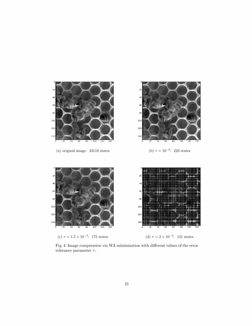
We have applied our image compression tool to some images. Figure 4a showsa picture with a resolution of 150 × 150 pixels. The weighted automaton thatencodes the image exactly has 33110 states. Applying minimisation with errortolerance parameter τ = 10−6 yields an automaton with 229 states, which leadsto the compressed picture in Figure 4b. Larger values of τ lead to smaller au-tomata and blurrier pictures, see Figures 4c and 4d, where the pictures changeperceivably.
We remark that our tool is not meant to deliver state-of-the-art image com-pression, which would require many tweaks, as indicated in [15].
20
(a) original image: 33110 states (b) τ = 10−6: 229 states
(c) τ = 1.5× 10⁻²: 175 states (d) τ = 2× 10⁻²: 121 states
Fig. 4: Image compression via WA minimisation with different values of the errortolerance parameter τ .
21

B Proofs of Section 4
B.1 Continuation of the proof of Proposition 6
Proposition 6. The restricted hypercube problem can in polynomial time bereduced to the PA minimisation problem.
Proof. Consider the reduction given in the main body of the paper. Observethat we have for all i ∈ {2, . . . , k} and all s ∈ Nd that
LA(aibs) = M(ai)[1, i] M(bs)[i, k + 1] = pi[s] . (16)
It remains to show the correctness of the reduction, i.e., we need to show thatthere is a set Q = {q1, . . . , q`} ⊆ [0, 1]d with conv(Q) ⊇ P if and only if there isa PA A′ = (`+ 1, Σ,M ′, α′, η′) equivalent to A.
For the “only if” direction, suppose that Q = {q1, . . . , q`} such thatconv(Q) ⊇ P . As p1 = (0, . . . , 0) ∈ P is a vertex of the hypercube, we havep1 ∈ Q, say q1 = (0, . . . , 0). As conv(Q) ⊇ P , for each i ∈ {2, . . . , k} there are
λ(i)1 , . . . , λ
(i)` ≥ 0 with
∑`j=1 λ
(i)j = 1 and
pi =∑j=1
λ(i)j qj =
∑j=2
λ(i)j qj . (17)
Build the PA A′ = (` + 1, Σ,M ′, α′, η′) as follows. Set M ′(ai)[1, j] := λ(i)j and
M ′(bs)[j, `+1] := qj [s] for all i ∈ {2, . . . , k} and all j ∈ {2, . . . , `} and all s ∈ Nd,and set all other entries of M ′ to 0. Set α′ := e(1) and η′ := e(` + 1)T . ThenA,A′ are equivalent, as
LA(aibs)(16)= pi[s]
(17)=∑j=2
λ(i)j qj [s] =
∑j=2
M ′(ai)[1, j] M′(bs)[j, `+ 1] = LA′(aibs) .
For the “if direction”, suppose that A′ = (` + 1, Σ,M ′, α′, η′) is a PA withLA′ = LA. For any vector β ∈ [0, 1]`+1 we define supp(β) := {j ∈ N`+1 | β[j] >0}. Define the following subsets of N`+1:
J1 := supp(α′) ∩⋃
i∈{2,...,k}, s∈Nd
supp (M ′(ai)M′(bs)η
′)
J2 :=⋃
i∈{2,...,k}
supp (α′M ′(ai)) ∩⋃s∈Nd
supp (M ′(bs)η′)
J3 :=⋃
i∈{2,...,k}, s∈Nd
supp (α′M ′(ai)M′(bs)) ∩ supp(η′)
Recall that LA′ = LA. Since LA(bs) = 0 for all s, we have J1 ∩ J2 = ∅. SinceLA(τ) = 0, we have J1 ∩ J3 = ∅. Since LA(ai) = 0 for all i, we have J2 ∩ J3 = ∅.If one of J1, J2, J3 is the empty set, then J1 = J2 = J3 = ∅ and we have
22

LA(w) = 0 for all w ∈ Σ∗, so then by (16) we have P = {(0, . . . , 0)}, and onecan take Q = P . So we can assume for the rest of the proof that J1, J2, J3 areall non-empty. But they are pairwise disjoint, so it follows |J2| ≤ `− 1. Without
loss of generality, assume 1 6∈ J2. For i ∈ {2, . . . , k} and j ∈ J2, define λ(i)j ≥ 0
and qj ∈ [0, 1]d with
λ(i)j = (α′M ′(ai)) [j] and qj [s] = (M ′(bs)η
′) [j] for s ∈ Nd.
Let q1 := (0, . . . , 0). Since α′M ′(ai) is stochastic, one can choose λ(i)1 ≥ 0 so that∑
j∈{1}∪J2 λ(i)j = 1. We have:
pi[s](16)= LA(aibs) = LA′(aibs) = α′M ′(ai)M
′(bs)η′
=∑j∈J2
(α′M ′(ai)) [j] (M ′(bs)η′) [j] =
∑j∈{1}∪J2
λ(i)j qj [s]
It follows that P ⊆ conv(Q) holds for Q := {qj | j ∈ {1}∪J2}, with |Q| ≤ `. ut
B.2 Proof of Proposition 8
Proposition 8. The hypercube problem is NP-hard. This holds even for therestricted hypercube problem.
Proof. We reduce 3SAT to the hypercube problem. Let x1, . . . , xN be the vari-ables and let ϕ = c1 ∧ . . . ∧ cM be a 3SAT formula. Each clause cj is a disjunc-tion of three literals cj = lj,1 ∨ lj,2 ∨ lj,3, where lj,k = x−j,k or lj,k = x+j,k andxj,k ∈ {x1, . . . , xN}. (It is convenient in the following to distinguish between avariable and a positive literal, so we prefer the notation x−i and x+i over themore familiar ¬xi and xi for literals.) We can assume that no clause appearstwice in ϕ and that no variable appears twice in the same clause. Define a setD of coordinates:
D := {x∗i , yi, zi | i ∈ NN} ∪ {c∗j | j ∈ NM}
We take d := |D| = 3N + M . For u ∈ D denote by e(u) ∈ {0, 1}D the vectorwith e(u)[u] = 1 and e(u)[u′] = 0 for u′ ∈ D\{u}. For i ∈ NN , define shorthandsf(x−i ) := e(yi) and f(x+i ) := e(yi)+e(zi). Observe that those points are verticesof the hypercube.
23
Define:
Pvar := {e(x∗i ) + f(x−i ), e(x∗i ) + f(x+i ) | i ∈ NN}Pcla := {e(c∗j ) + f(lj,1), e(c∗j ) + f(lj,2), e(c∗j ) + f(lj,3) | j ∈ NM}
p(xi) :=1
2e(x∗i ) + e(yi) +
1
2e(zi)
=1
2e(x∗i ) +
1
2f(x−i ) +
1
2f(x+i ) for i ∈ NN
p(cj) :=2
3e(c∗j ) +
1
3f(lj,1) +
1
3f(lj,2) +
1
3f(lj,3) for j ∈ NM
P := Pvar ∪ Pcla ∪ {p(x1), . . . , p(xN ), p(c1), . . . , p(cM )}
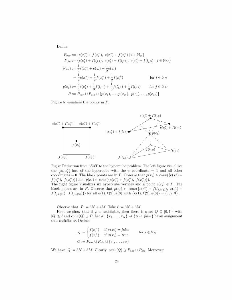
Figure 5 visualizes the points in P .
f(x−i ) f(x+i )
p(xi)
e(x∗i ) + f(x−i ) e(x∗i ) + f(x+i )e(c∗j ) + f(lj,1)
e(c∗j ) + f(lj,2)
e(c∗j ) + f(lj,3) p(cj)
f(lj,1)f(lj,2)
f(lj,3)
Fig. 5: Reduction from 3SAT to the hypercube problem. The left figure visualizesthe {zi, x∗i }-face of the hypercube with the yi-coordinate = 1 and all othercoordinates = 0. The black points are in P . Observe that p(xi) ∈ conv({e(x∗i ) +f(x−i ), f(x+i )}) and p(xi) ∈ conv({e(x∗i ) + f(x+i ), f(x−i )}).The right figure visualizes six hypercube vertices and a point p(cj) ∈ P . Theblack points are in P . Observe that p(cj) ∈ conv({e(c∗j ) + f(lj,k(1)), e(c
∗j ) +
f(lj,k(2)), f(lj,k(3))}) for all k(1), k(2), k(3) with {k(1), k(2), k(3)} = {1, 2, 3}.
Observe that |P | = 3N + 4M . Take ` := 3N + 3M .First we show that if ϕ is satisfiable, then there is a set Q ⊆ [0, 1]d with
|Q| ≤ ` and conv(Q) ⊇ P . Let σ : {x1, . . . , xN} → {true, false} be an assignmentthat satisfies ϕ. Define:
si :=
{f(x−i ) if σ(xi) = false
f(x+i ) if σ(xi) = truefor i ∈ NN
Q := Pvar ∪ Pcla ∪ {s1, . . . , sN}
We have |Q| = 3N + 3M . Clearly, conv(Q) ⊇ Pvar ∪ Pcla . Moreover:
24

– Let i ∈ NN . If σ(xi) = false, then p(xi) = 12
(e(x∗i ) + f(x+i )
)+ 1
2si; if
σ(xi) = true, then p(xi) = 12
(e(x∗i ) + f(x−i )
)+ 1
2si.– Let j ∈ NM . As σ satisfies ϕ, there are k(1), k(2), k(3) such that{k(1), k(2), k(3)} ∈ {1, 2, 3} and σ(lj,k(1)) = true. Let i ∈ NN such that
lj,k(1) ∈ {x−i , x+i }. Then p(cj) = 1
3
(e(c∗j )+f(lj,k(2))
)+ 1
3
(e(c∗j )+f(lj,k(3))
)+
13si.
Hence we have that conv(Q) ⊇ P .For the converse, let Q ⊆ [0, 1]d with |Q| ≤ 3N + 3M and conv(Q) ⊇ P .
Then Q ⊇ Pvar ∪ Pcla, as Pvar and Pcla consist of hypercube vertices.Let i ∈ NN . Let Qvar
i ⊆ Q be a minimal subset of Q with p(xi) ∈ conv(Qvari ),
i.e., if Q′i is a proper subset of Qvari , then p(xi) 6∈ conv(Q′i). As p(xi)[x
∗i′ ] =
p(xi)[c∗j ] = 0 holds for all i′ ∈ NN \ {i} and all j ∈ NM , we have
Qvari ∩ (Pvar ∪ Pcla) ⊆ {e(x∗i ) + f(x−i ), e(x∗i ) + f(x+i )} .
As p(xi)[x∗i ] = 1
2 and p(xi)[yi] = 1, there is a point si ∈ Qvari with si[x
∗i ] ≤ 1
2and si[yi] = 1 and si[zi] ∈ [0, 1] and si[u] = 0 for all other coordinates u ∈ D.
It follows that Q = Pvar ∪Pcla ∪ {s1, . . . , sN} and |Q| = 3N + 3M . Let σ beany assignment with
σ(xi) =
{false if si[zi] = 0
true if si[zi] = 1 .
We show that σ satisfies ϕ. Let j ∈ NM . Let Qclaj ⊆ Q be a minimal subset
of Q with p(cj) ∈ conv(Qclaj ), i.e., if Q′j is a proper subset of Qcla
j , then p(cj) 6∈conv(Q′j). As p(cj)[c
∗j′ ] = p(cj)[x
∗i ] = 0 holds for all j′ ∈ NM \{j} and all i ∈ NN ,
we have
Qclaj ⊆ {e(c∗j ) + f(lj,1), e(c∗j ) + f(lj,2), e(c∗j ) + f(lj,3)} ∪ {s1, . . . , sN} .
As p(cj)[c∗j ] = 2
3 < 1, there exists an i such that si ∈ Qclaj . As si[yi] = 1 > 0, we
have p(cj)[yi] > 0. Hence the variable xi appears in cj , so one of the followingtwo cases holds:
– The literal x−i appears in cj . As we have p(cj)[zi] = 0, it follows that q[zi] = 0holds for all q ∈ Qcla
j . In particular, we have si[zi] = 0, so σ(xi) = false.
– The literal x+i appears in cj . Note that for all points q ∈ Qclaj we have
q[yi] ≥ q[zi]. As we have p(cj)[yi] = 13 = p(cj)[zi], it follows that q[yi] = q[zi]
holds for all q ∈ Qclaj . In particular, we have si[zi] = 1, so σ(xi) = true.
For both cases it follows that σ satisfies cj . As j was chosen arbitrarily, we con-clude that σ satisfies ϕ. This completes the reduction to the hypercube problem.
The given reduction does not put the origin in P . However, Pvar ∪ Pcla ⊆ Pconsist of corners of the hypercube. One can pick one of the corners in P andapply a simple linear coordinate transformation to all points in P such that thepicked corner becomes the origin. Hence the restricted hypercube problem isNP-hard as well. ut
25

B.3 Proof of Proposition 10
Proposition 10. Let A1 = (n1, Σ,M1, α1, η1) be a PA. A PAA2 = (n2, Σ,M2, α2, η2) is equivalent to A1 if and only if there exist matrices−→M(a) ∈ R(n1+n2)×(n1+n2) for a ∈ Σ and a matrix F ∈ R(n1+n2)×(n1+n2) suchthat F [1, ·] = (α1, α2), and F (ηT1 ,−ηT2 )T = (0, . . . , 0)T , and
F
(M1(a) 0
0 M2(a)
)=−→M(a)F for all a ∈ Σ.
Proof. We say, a WA A is zero if LA(w) = 0 holds for all w ∈ Σ∗. For twoWAs Ai = (ni, Σ,Mi, αi, ηi) (with i = 1, 2), define their difference WA A =
(n,Σ,M,α, η), where n = n1 +n2, and M(a) =
(M1(a) 0
0 M2(a)
)for a ∈ Σ, and
α = (α1, α2), and η = (ηT1 ,−ηT2 )T . Clearly, LA(w) = LA1(w) − LA2
(w) holdsfor all w ∈ Σ∗. So WAs A1 and A2 are equivalent if and only if their differenceWA is zero.
A WA A = (n,Σ,M,α, η) is zero if and only if all vectors of the forwardspace 〈αM(w) | w ∈ Σ∗〉 are orthogonal to η (see, e.g., [26]). It follows that aWA A = (n,Σ,M,α, η) is zero if and only if there is a vector space F ⊆ Rn withα ∈ F, and Fη = {0}, and FM(a) ⊆ F holds for all a ∈ Σ. (Here, the actualforward space is a subset of F.)
The proposition follows from those observations. ut
26