stabilization and trajectory tracking control for

Sadhana Vol. 40, Part 5, August 2015, pp. 1531–1553. c© Indian Academy of Sciences

Stabilization and trajectory tracking control for

underactuated quadrotor helicopter subject to wind-gust

disturbance

MOHD ARIFFANAN MOHD BASRI∗, ABDUL RASHID HUSAIN

and KUMERESAN A DANAPALASINGAM

Department of Control and Mechatronics Engineering, Faculty of Electrical

Engineering, Universiti Teknologi Malaysia, 81310 Skudai, Johor, Malaysia

e-mail: [email protected]

MS received 20 April 2014; revised 2 December 2014; accepted 24 February 2015

Abstract. The control of quadrotor helicopter has been a great challenge for control

engineers and researchers since quadrotor is an underactuated and a highly unstable

nonlinear system. In this paper, the dynamic model of quadrotor has been derived and

a so-called robust optimal backstepping control (ROBC) is designed to address its sta-

bilization and trajectory tracking problem in the existence of external disturbances.

The robust controller is achieved by incorporating a prior designed optimal backstep-

ping control (OBC) with a switching function. The control law design utilizes the

switching function in order to attenuate the effects caused by external disturbances. In

order to eliminate the chattering phenomenon, the sign function is replaced by the sat-

uration function. A new heuristic algorithm namely Gravitational Search Algorithm

(GSA) has been employed in designing the OBC. The proposed method is evaluated

on a quadrotor simulation environment to demonstrate the effectiveness and merits of

the theoretical development. Simulation results show that the proposed ROBC scheme

can achieve favorable control performances compared to the OBC for autonomous

quadrotor helicopter in the presence of external disturbances.

Keywords. Quadrotor helicopter; robust control; backstepping control; gravitational

search algorithm.

1. Introduction

Currently, the interest for vertical take-off and landing (VTOL) vehicles is strongly increasing.

This is due to their ability to hover flight and their lack of necessity for runways make them well-

suited options for supervision, inspection, and work in environments where space is limited and

high maneuverability is required. The quadrotor is a four-rotor VTOL vehicle which has sev-

eral advantages over traditional helicopters in terms of maneuverability, motion control and cost.

∗For correspondence

1531

1532 Mohd Ariffanan Mohd Basri et al

However, quadrotors are inherently unstable, nonlinear, multivariable and underactuated sys-

tems. Hence, the control of a quadrotor becomes quite a complex and difficult mainly due to its

underactuated properties and nonlinearities. In literature, different studies have addressed mod-

eling and control of underactuated nonlinear systems and variety of approaches are employed

(Zilic et al 2013; Yih 2013; Xu et al 2012; Yang & Yang 2012; Yu et al 2012).

To solve the quadrotor helicopter control problem, many techniques have been proposed

such as linear quadratic regulator (LQR) control (Nuchkrua & Parnichkun 2012; Jafari et al

2010; Castillo et al 2005), proportional-integral-derivative (PID) control (Junior et al 2013;

Bolandi et al 2013; Hwang et al 2012), fuzzy logic (FL) control (Baek et al 2013; Erginer &

Altug 2012; Santos et al 2010), feedback linearization control (Zhang et al 2013; Mukherjee &

Waslander 2012; Mokhtari et al 2006), sliding mode control (Sumantri et al 2013; Guisser &

Medromi 2009; Bouadi et al 2007) and backstepping control (Lee et al 2013; Regula & Lantos

2011; Madani & Benallegue 2006). Initially, most of the control strategies are based on lin-

earized models without compensation of modeling errors and external disturbances. Then, in the

past few years, more efforts have been directed toward the research of dealing with uncertainties

and disturbances associated with nonlinear quadrotor dynamic model.

In this paper, the control problem of the quadrotor helicopter in the presence of external dis-

turbances is considered. The dynamical model describing the quadrotor helicopter motions and

taking into account for various parameters which affect the dynamics of a flying structure is

presented. Subsequently, a control strategy based on backstepping approach taking into account

the external disturbances is developed. The backstepping control scheme is a nonlinear con-

trol method based on the Lyapunov theorem. The backstepping control design techniques have

received great attention because of its systematic and recursive design methodology for non-

linear feedback control. The backstepping control approach has been successfully implemented

in various forms to numerous real-world applications such as satellite (Kristiansen et al 2009),

suspension systems (Sun et al 2013), aircraft (Shen et al 2013), chemical reactor (Boškovic &

Krstic 2002), flexible spacecraft (Jiang et al 2010), robot manipulator (Hu et al 2012), electro-

hydraulic actuator (Kim et al 2010), and wheeled inverted pendulum systems (Chiu et al 2011).

The advantage of backstepping compared with other control methods lies in its design flexibil-

ity, due to its recursive use of Lyapunov functions. The key idea of the backstepping design is

to select recursively some appropriate state variables as virtual inputs for lower dimension sub-

systems of the overall system and the Lyapunov functions are designed for each stable virtual

controller (Krstic et al 1995). Therefore, the final designed actual control law can guarantee the

stability of total control system.

Although the nonlinear control realized by backstepping method can meet the desired per-

formance of the system, it is just limited to the nominal system i.e. the system dynamics and

the external disturbance are exactly known. To overcome this drawback, a nominal controller

based on backstepping technique combined with a switching function is proposed to deal with

the control problem of the quadrotor helicopter under the influence of external disturbances.

Compared with the only backstepping control scheme (Madani & Benallegue 2006), the present

control approach has the advantages of robust control, which makes this approach attractive

for a wide class of nonlinear systems with the influences of external disturbances. To solve the

problem of determining the control design parameters, Gravitational Search Algorithm (GSA)

has been used. Finally, the synthesized control law is highlighted by simulations which gave

fairly satisfactory results despite the occurrence of external disturbances. The main contribution

of this paper is a successful development of a new backstepping-based nonlinear control struc-

ture for quadrotor helicopter perturbed by external disturbances. Unlike the method presented in

Stabilization and tracking control of quadrotor helicopter 1533

Bouadi et al (2008), the developed control scheme has the advantage of free from the chattering

phenomena.

2. Quadrotor systems modeling

2.1 Quadrotor description

The quadrotor helicopter, shown in figure 1, has four rotors to generate the propeller forces Fi =

1, 2, 3, 4. The four rotors can be thought of as two pairs, (1,3)@(front, back) and (2,4)@(left,

right). One pair rotates clockwise, while the other rotates counter clockwise in order to balance

the torques and produce yaw motion as needed. Yaw motion can be obtained from the difference

in the counter torque between each pair of propellers, (1,3) and (2,4). When all four rotors

are spinning with the same angular velocity the net yaw is zero, and a difference in velocities

between the two pairs creates either positive or negative yaw motion. The up (down) motion

can be achieved by increasing (decreasing) the rotor speeds altogether with the same magnitude.

Forward (backward) motion which is related to the pitch, θ angle can be obtained by increasing

the back (front) rotor thrust and decreasing the front (back) rotor thrust. Finally, a sideways

motion which is related to the roll, φ angle can be achieved by increasing the left (right) rotor

thrust and decreasing the right (left) rotor thrust. Figure 2 shows the various movements of a

quadrotor due to changes in rotor speeds.

In order to develop the model of the quadrotor, reasonable assumptions are established in

order to accommodate the controller design. The assumptions are as follows:

Assumption 1: Quadrotor is a rigid body and has symmetric structure.

Assumption 2: Aerodynamic effects can be ignored at low speed.

Assumption 3: The rotor dynamics are relatively fast and thus can be neglected.

Assumption 4: The quadrotor’s center of mass and body-fixed frame origin coincide.

xe

B

zb

yb xb

F1F2

F3 F4

ze

ye

E

Figure 1. Quadrotor helicopter configuration.


Rotate Clockwise

Rotate Counterclockwise Move Forward Move Right Move Upward

Move Backward Move Left Move Downward

4

1

2

3

Figure 2. The movements of a quadrotor: the arrow width is proportional to rotor speeds.

2.2 Quadrotor kinematic model

Consider earth fixed frame E = {xe, ye, ze} and body fixed frame B = {xb, yb, zb}, as seen in

figure 1. Let q = (x, y, z, φ, θ, ψ) ∈ R6 be the generalized coordinates for the quadrotor,

where (x, y, z) denote the absolute position of the rotorcraft and (φ, θ, ψ) are the three Euler

angles (roll, pitch and yaw) that describe the orientation of the aerial vehicle. Therefore, the

model could be separated into two coordinate subsystems: translational and rotational. They are

defined respectively by

ξ = (x, y, z) ∈ R3 (1)

η = (φ, θ, ψ) ∈ R3. (2)

The kinematic equations of the translational and rotational movements are obtained by means

of the rotation R and transfer T matrices, respectively. The expression of the rotation R and

transfer T matrices can be found in Olfati-Saber (2000) and defined accordingly by (3) and (4):

R =

⎛

⎝

cθcψ sφsθcψ − cφsψ cφsθcψ + sφsψ

cθsψ sφsθsψ + cφcψ cφsθsψ − sφcψ

−sθ sφcθ cφcθ

⎞

⎠ (3)

T =

⎛

⎝

1 sφtθ cφtθ

0 cφ −sφ

0 sφ/cθ cφ/cθ

⎞

⎠ , (4)

where s(·), c(·) and t (·) are abbreviations for sin(·), cos(·) and tan(·), respectively.

The translational kinematic can be written as

ξ = RV, (5)

where ξ and V are, respectively, the linear velocity vector w.r.t. the earth fixed frame E and body

fixed frame B.


The rotational kinematics can be defined as follows:

η = T ω, (6)

where η and ω are the angular velocity vector w.r.t. the earth fixed frame E and body fixed frame

B, respectively.

2.3 Quadrotor dynamic model

The dynamic model of quadrotor is derived from Newton–Euler approach. It can be useful to

express the translational dynamic equations w.r.t. the earth fixed frame E and rotational dynamic

equations w.r.t. the body fixed frame B.

Therefore, the translational dynamic equations of quadrotor can be written as follows:

mξ = −mgez + uT Rez, (7)

where m denotes the quadrotor mass, g the gravity acceleration, ez = (0, 0, 1)T the unit vector

expressed in the frame E and uT the total thrust produced by the four rotors.

uT =∑4

i=1Fi = b

∑4

i=1�2

i , (8)

where Fi and �i denote respectively, the thrust force and speed of the rotor i and b is the thrust

factor.

The rotational dynamic equations of quadrotor can be written as follows:

I ω = −ω × Iω − Ga + τ, (9)

where I is the inertia matrix, −ω×Iω and Ga are the gyroscopic effect due to rigid body rotation

and propeller orientation change respectively, while τ is the control torque obtained by varying

the rotor speeds. Ga and τ are defined as

Ga =∑4

i=1Jr(ω × ez)(−1)i+1�i (10)

τ =

⎛

⎝

τφ

τθ

τψ

⎞

⎠ =

⎛

⎜

⎝

lb(

�24 − �2

2

)

lb(

�23 − �2

1

)

d(

�22 + �2

4 − �21 − �2

3

)

⎞

⎟

⎠, (11)

where Jr is the rotor inertia, l represents the distance from the rotors to the centre of mass and d

is the drag factor.

Then, by recalling (7) and (9), the dynamic model of the quadrotor in terms of position

(x, y, z) and rotation (φ, θ, ψ) is written as⎛

⎝

x

y

z

⎞

⎠ =

⎛

⎝

0

0

−g

⎞

⎠ +1

m

⎛

⎝

cφsθcψ + sφsψcφsθ sψ − sφcψ

cφcθ

⎞

⎠ uT (12)

⎛

⎝

φ

θ

ψ

⎞

⎠ =

⎛

⎜

⎜

⎜

⎝

θ ψ(

Iyy−Izz

Ixx

)

φψ(

Izz−Ixx

Iyy

)

θ φ(

Ixx−Iyy

Izz

)

⎞

⎟

⎟

⎟

⎠

−

⎛

⎜

⎝

Jr

Ixxθ�d

− Jr

Iyyφ�d

0

⎞

⎟

⎠+

⎛

⎜

⎜

⎝

1Ixx

τφ

1Iyy

τθ

1Izz

τψ

⎞

⎟

⎟

⎠

. (13)


Consequently, quadrotor is an underactuated system with six outputs (x, y, z, φ, θ, ψ) and

four control inputs (uT , τφ, τθ , τψ ).

Finally, the quadrotor dynamic model can be written in the following form:

x = (cφsθcψ + sφsψ )1

mu1

y = (cφsθ sψ − sφcψ )1

mu1

z = −g + (cφcθ )1

mu1

φ = θ ψ

(

Iyy − Izz

Ixx

)

−Jr

Ixx

θ�d +l

Ixx

u2

θ = φψ

(

Izz − Ixx

Iyy

)

+Jr

Iyy

φ�d +l

Iyy

u3

ψ = θ φ

(

Ixx − Iyy

Izz

)

+1

Izz

u4 (14)

with a renaming of the control inputs as

u1 = b(

�21 + �2

2 + �23 + �2

4

)

u2 = b(

�24 − �2

2

)

u3 = b(

�23 − �2

1

)

u4 = d(

�22 + �2

4 − �21 − �2

3

)

(15)

and the �d is formulated as

�d = �2 + �4 − �1 − �3. (16)

3. Backstepping control system for quadrotor

The dynamic model (14) with the consideration of external disturbance can be represented into

nonlinear dynamic equation described as follows:

X = f (X) + g(X)u + δ, (17)

where u, X and δ are respectively the input, state and external disturbance vector given as

follows:

u = [u1 u2 u3 u4]T (18)

X = [x1 x2 x3 x4 x5 x6]T = [z φ θ ψ x y]T (19)

δ = [δ1 δ2 δ3 δ4 δ5 δ6]T . (20)


The bound of the external disturbance is assumed to be given, that is |δ| ≤ β, where β is a

given positive constant. From (14) and (19), the nonlinear dynamic function f (X) and nonlinear

control function g (X) matrices can be written accordingly as

f (X) =

⎛

⎜

⎜

⎜

⎜

⎜

⎜

⎝

−g

θψa1 − θa2�d

φψa3 + φa4�d

θ φa5

0

0

⎞

⎟

⎟

⎟

⎟

⎟

⎟

⎠

g (X) =

⎛

⎜

⎜

⎜

⎜

⎜

⎜

⎝

uz1m

0 0 0

0 b1 0 0

0 0 b2 0

0 0 0 b3

ux1m

0 0 0

uy1m

0 0 0

⎞

⎟

⎟

⎟

⎟

⎟

⎟

⎠

(21)

with the abbreviations a1 =(

Iyy − Izz

)

/Ixx , a2 = Jr/Ixx , a3 = (Izz − Ixx) /Iyy , a4 = Jr/Iyy ,

a5 =(

Ixx − Iyy

)

/Izz, b1 = l/Ixx , b2 = l/Iyy , b3 = 1/Izz, uz =(

cφcθ

)

The control objective is to design a suitable control law for the system (17) so that the state

trajectory X can track a desired reference trajectory Xd = [x1d x2d x3d x4d x5d x6d ]T despite

the presence of external disturbance. Since the description of the control system design of the

helicopter is similar for each DOF, for simplicity only one of the six DOF is considered.

The design of ideal backstepping control (IBC) is described step-by-step as follows:

Step 1: Define the tracking error:

e1 = x1d − x1, (22)

where x1d is a desired trajectory specified by a reference model. Then the derivative of tracking

error can be represented as

e = x1d − x1. (23)

The first Lyapunov function is chosen as

V1(e1) =1

2e2

1. (24)

The derivative of V1 is

V1(e1) = e1e1 = e1(x1d − x1). (25)

x1 can be viewed as a virtual control. The desired value of virtual control known as a stabilizing

function can be defined as follows:

α1 = x1d + k1e1, (26)

where k1 is a positive constant and should be determined by the GSA.

By substituting the virtual control by its desired value, Eq. (25) then becomes

V1(e1) = −k1e21 ≤ 0. (27)

Step 2: The deviation of the virtual control from its desired value can be defined as

e2 = x1 − α1 = x1 − x1d − k1e1. (28)


The derivative of e2 is expressed as

e = x1 − α1

= f (x1) + g(x1)u1 + δ1 − x1d − k1e1. (29)

The second Lyapunov function is chosen as

V2(e1, e2) =1

2e2

1 +1

2e2

2. (30)

Finding derivative of (30) yields

V2(e1, e2) = e1e1 + e2e2

= e1(x1d − x1) + e2(x1 − α1)

= e1(−e2 − k1e1) + e2(f (x2) + g(x1)u1 + δ1 − x1d − k1e1)

= −k1e21 + e2(−e1 + f (x1) + g(x1)u1 + δ1 − x1d − xd − k1e1). (31)

Step 3: Assuming the external disturbance is well known, an IBC can be obtained as

u1(IB) =1

g(x1)(e1 + k1e1 + x1d − f (x1) − δ1 − k2e2), (32)

where k2 is a positive constant and should be also determined by the GSA. The term k2e2 is

added to stabilize the tracking error e1.

Substituting (32) into (31), the following equation can be obtained:

V2(e1, e2) = −k1e21 − k2e

22 = −ET KE ≤ 0, (33)

where E = [e1 e2]T and K = diag (k1, k2). Since V2 (e1, e2) ≤ 0, V2 (e1, e2) is negative

semi-definite.

Therefore, the IBC in (32) will asymptotically stabilize the system.

4. Backstepping control parameters optimization

4.1 Overview of gravitational search algorithm

The gravitational search algorithm (GSA) is one of the newest heuristic algorithms inspired by

the Newtonian laws of gravity and motion developed by Rashedi et al (2009). In this algorithm,

agents are considered as objects and their performance is measured by their masses. All these

objects attract each other by the gravity force, and this force causes a global movement of all

objects towards the objects with heavier masses. The heavy masses correspond to good solutions

and move more slowly than lighter ones representing worse solutions. The position of the mass

corresponds to a solution of the problem, and its gravitational and inertial masses are determined

using a fitness function.

Consider an optimization problem of d dimension and N agents (masses). The position of the

ith agent is defined as follows:

Xi = (x1i , x2

i , . . . , xdi ) for i = 1, 2, . . . , N. (34)

The gravitational force between agents i and j at time t is represented as follows:

F dij (t) = G(t)

Mi(t) × Mj (t)

Rij (t) + ε

(

xdj (t) − xd

i (t))

, (35)


where Mi is the mass of the agent i, Mj is the mass of the agent j , G(t) the gravitational constant

at time t , ε a small constant and Rij (t) is the Euclidian distance between agent i and j objects

defined as follows:

Rij (t) = ‖Xi(t), Xj (t)‖2. (36)

The gravitational constant, G is initialized at the beginning and will be reduced with time to

control the search accuracy. In other words, G is a function of the initial value G0 and time t

given as follows:

G(t) = G(G0, t). (37)

The total force acting on the ith agent is calculated as follows:

F di (t) =

N∑

j=1,j �=1

randjFdij (t), (38)

where randj is a random number in the interval [0,1].

According to Newton’s law of motion, the acceleration of the agent i at time t in the d

dimension is given as follows:

adi (t) =

F di (t)

Mi(t), (39)

where

Mi(t) =mi(t)

∑Nj=1mj (t)

(40)

and

mi(t) =fiti(t) − worst(t)

best(t) − worst(t), (41)

where fiti(t) represents the fitness value of the agent i at time t , best(t) and worst(t) are respec-

tively the best fitness value and the worst fitness value of agent i at time t .

It is to be noted that for a minimization problem:

best(t) = min(fiti(t)) i = 1, 2, . . . , N (42)

worst(t) = max(fiti(t)) i = 1, 2, . . . , N. (43)

The updated velocity of an agent is defined as a function of its current velocity added to its

current acceleration. Hence, the next position and next velocity of an agent can be formulated as

follows:

νdi (t + 1) = randi × νd

i (t) + adi (t) (44)

xdi (t + 1) = xd

i (t) + νdi (t + 1). (45)

where νdi and xd

i (t) are the velocity and position of an agent at t time in d dimension,

respectively. randi is a random number in the interval [0,1].


4.2 Optimal backstepping control system

The dynamic model in (14) can be divided into two subsystems �1 and �2, listed as follows:

�1 :

⎧

⎪

⎪

⎪

⎨

⎪

⎪

⎪

⎩

φ = θ ψ(

Iyy−Izz

Ixx

)

− Jr

Ixxθ�d + l

Ixxu2

θ = φψ(

Izz−Ixx

Iyy

)

+ Jr

Iyyφ�d + l

Iyyu3

ψ = θ φ(

Ixx−Iyy

Izz

)

+ lIzz

u4

(46)

�2 :

⎧

⎪

⎨

⎪

⎩

x = (cφsθcψ + sφsψ) 1m

u1

y = (cφsθsψ − sφcψ) 1m

u1

z = −g + (cφcθ) 1m

u1

. (47)

�1 in (46) represents the rotation subsystem related to the dynamics of quadrotor roll motion

φ, pitch motion θ and yaw motion ψ . �2 in (47) represents the position subsystem related to

the dynamics of quadrotor longitude motion x, latitude motion y and altitude motion z. Hence,

the control scheme advocated for the overall system is then logically divided into a rotation

controller and a position controller. In the previous section a controller (32) has been designed to

stabilize one DOF of the overall system. The coefficients k1, k2 are control parameters and need

to be positive to satisfy stability criteria. In conventional backstepping method, these parameters

are selected by trial and error. It is also possible that the parameters are properly chosen, but it

cannot be said that the optimal parameters are selected. To overcome this drawback, this paper

adopts the GSA for determining the optimal value of the backstepping control parameters. The

GSA is utilized off line to determine the backstepping controller parameters. The performance

of the controller varies according to adjusted parameters. Since the optimal backstepping control

(OBC) aims to improve the control performance yielded by a backstepping controller, it keeps

the simple structure of the backstepping controller. As aforementioned, each of the rotation and

position subsystem is comprised of three DOF. Then there are in sum six control parameters that

need to be selected simultaneously for each subsystem.

In the present study, an integral absolute error (IAE) is utilized to judge the performance of the

controller. IAE criterion is widely adopted to evaluate the dynamic performance of the control

system. The index IAE is expressed as follows (De Moura Oliveira et al 2013):

IAE =

t∫

0

|e(t)|dt. (48)

Since the system is comprised of two subsystems, a vector integral absolute error for the rota-

tion subsystem is taken as IAER = [IAEφ IAEθ IAEψ ], where the subscripts are denoted for

roll, pitch and yaw, respectively. Meanwhile, a vector integral absolute error for the position sub-

system is taken as IAEp = [IAEx IAEy IAEz], where the subscripts are denoted for longitude,

latitude and altitude, respectively.

For the rotation controller, GSA is utilized to minimize the fitness function JR , expressed as

JR = IAER · W (49)

and for the position controller, GSA is utilized to minimize the fitness function JP , expressed as

JP = IAEP · W, (50)


where W = [W1 W2 W3]T is weighting vector used to set the priority of the multiple objective

performance index (MOPI) parameters and the value of “W” varies from 0 to 1. In this case,

equal weights for the three objectives to be met by the each controller are considered as such

the minimizations of the error indexes are equally important. For fitness function calculation, the

time-domain simulation of the quadrotor system model is carried out for the simulation period,

t . It is aimed to minimize this fitness function in order to improve the system response in terms

of the steady-state errors.

5. Robust optimal backstepping control system

However, if unpredictable perturbations from the external disturbance occur, the optimized IBC

(32) effort cannot ensure the favorable control performance. Thus, auxiliary control effort should

be designed as switching control effort to eliminate the effect of the unpredictable perturbations.

The auxiliary control effort is referred as switching control effort defined as follows:

u1(sw) = λsign(e2), (51)

where λ is a constant determined by design parameter and sign(e2) is a sign function:

sign(e2) =

{

1, e2/ρ > 0

−1, e2/ρ < 0.(52)

The backstepping control effort for the nominal model (δ = 0) is formulated as follows:

u1(B) =1

g(x1)(e1 + k1e1 + x1d − f (x1) − k2e2). (53)

Totally, the robust optimal backstepping control (ROBC) law for one DOF of quadrotor nonlinear

systems with the present of external disturbance, which guarantees the stability and convergence

can be generally represented as

ui = ui(B) + ui(sw)

u1 =1

g (x1)(e1 +k1e1 + x1d −f (x1) − k2e2) +

ε

g (x1)sign(e2); (for i = 1), (54)

where ε is design parameter to be determined later.

The utilization of discontinuous switching function will excite undesired phenomenon called

chatter. In order to reduce the chattering phenomenon, the most common method is to utilize the

saturation function sat(e2/ρ). Thus, replacing sign(e2) by sat(e2/ρ) in (54) implies

u1 =1

g(x1)(e1 + k1e1 + x1d − f (x1) − k2e2 + εsat (e2/ρ)) . (55)

The saturation function sat (e2/ρ) is defined as follows:

sat(e2/ρ) =

{

sign(e2/ρ), |e2/ρ| > 1

e2/ρ, |e2/ρ| ≤ 1@ sat(e2/ρ) =

⎧

⎨

⎩

1, e2/ρ > 1

−1, e2/ρ < −1

e2/ρ, |e2/ρ| ≤ 1

, (56)

where ρ is a small positive constant.


Quadrotor

Stabilizing

Function

Backstepping

Control

GSA

Optimization

Figure 3. Block diagram of the robust optimal backstepping control system.

Theorem 1. For the nonlinear dynamic equation of quadrotor with external disturbance as

represented by (17), if the control law in (55) is applied, the system will be asymptotically stable.

Proof. Consider the following Lyapunov function:

V =1

2e2

1 +1

2e 2

2 . (57)

Differentiating (57) with respect to time leads to

V = e1e1 + e2e2

= e1(−e2 − k1e1) + e2(f (x1) + g(x1)u1 + δ1 − x1d − k1e1)

= −k1e21 + e2(−e1 + f (x1) + g(x1)u1 + δ1 − X1d − k1e1). (58)

Substituting the ROBC law from (55), then (58) becomes

V = −k1e21 − k2e

22 + e2(εsat(e2/ρ) + δ1)

= −k1e21 − k2e

22 + e2 + ε|e2| + δ1e2. (59)

From Lyapunov theorem, the system will be asymptotically stable if V is negative definite.

Hence, the design parameter should be chosen in such a way that V < 0 is always satisfied. As

aforementioned, it is assumed that δ is bounded with β. So, by choosing −ε ≥ β then V < 0

can be guaranteed.

The configuration of the proposed control system is depicted in figure 3. �

6. Simulation results

In this section, the performance of the proposed approach is evaluated. The corresponding algo-

rithm is implemented in MATLAB/SIMULINK simulation environment. The quadrotor system

is modeled in SIMULINK and the GSA is implemented in MATLAB. The model parameter

values of the quadrotor system are taken from Voos (2009) and listed in table 1. Initially, the

controller parameter optimization is searched with the quadrotor control model, and later the


Table 1. Parameters of the quadrotor.

Parameter Description Value Units

g Gravity 9.81 m/s2

m Mass 0.5 kgl Distance 0.2 m

Ixx Roll inertia 4.85 × 10−3 kg · m2

Iyy Pitch inertia 4.85 × 10−3 kg · m2

Izz Yaw inertia 8.81 × 10−3 kg · m2

b Thrust factor 2.92 × 10−6

d Drag factor 1.12 × 10−7

identified parameter values are transferred to the controller in the quadrotor system developed in

MATLAB/SIMULINK for further evaluation.

In this study, the following values are assigned for controller parameters optimization:

(i) Dimension of the search space = 6 (i.e., ki=1...6 or ki=7...12);

(ii) The number of agents (masses) = 15;

(iii) The number of maximum iteration = 20;

(iv) The searching ranges for the backstepping parameters are limited to [0, 15];

(v) The simulation time, t is equal to 10s;

(vi) Optimization process is repeated for 20 times.

The finest set of values among the simulation runs is selected as the best optimized controller

value. The parameter and fitness values of each particle during the simulation for the rotation and

position controller are summarized in tables 2 and 3, respectively. For the rotation controller, the

best fitness value is 4.933e − 008 appeared in iteration number 11, and the optimal parameters

are k1 = 14.00, k2 = 14.47, k3 = 15.00, k4 = 14.27, k5 = 14.29 and k6 = 14.62. The variation

Table 2. The rotation controller parameters and fitness value of each optimal particle.

Iteration no. Optimal parameters Fitness value

1 k1 = 12.22, k2 = 14.27 −4.503e − 006

k3 = 14.47, k4 = 14.82

k5 = 14.10, k6 = 14.13

3 k1 = 13.65, k2 = 12.94 −3.974e − 006

k3 = 14.98, k4 = 14.78

k5 = 12.27, k6 = 14.27

6 k1 = 12.00, k2 = 12.00 −4.327e − 007

k3 = 15.00, k4 = 14.52

k5 = 13.65, k6 = 14.47

11 k1 = 14.00, k2 = 14.47 −4.933e − 008

k3 = 15.00, k4 = 14.27

k5 = 14.29, k6 = 14.62

20 k1 = 14.00, k2 = 14.47 −4.933e − 008

k3 = 15.00, k4 = 14.27

k5 = 14.29, k6 = 14.62


Table 3. The position controller parameters and fitness value of each optimal particle.

Iteration no. Optimal parameters Fitness value

1 k7 = 14.66, k8 = 13.88 0.2476

k9 = 13.40, k10 = 13.14

k11 = 13.37, k12 = 14.33

2 k7 = 15.00, k8 = 13.77 0.2072

k9 = 13.64, k10 = 14.04

k11 = 13.77, k12 = 15.00

4 k7 = 15.00, k8 = 14.99 0.1599

k9 = 13.83, k10 = 14.41

k11 = 14.34, k12 = 15.00

7 k7 = 15.00, k8 = 15.00 0.1385

k9 = 14.29, k10 = 14.79

k11 = 14.70, k12 = 15.00

20 k7 = 15.00, k8 = 15.00 0.1385

k9 = 14.29, k10 = 14.79

k11 = 14.70, k12 = 15.00

of the fitness function with number of iterations is shown in figure 4. Meanwhile, the variations

of backstepping control parameters with respect to the number of iterations are shown in figure 5.

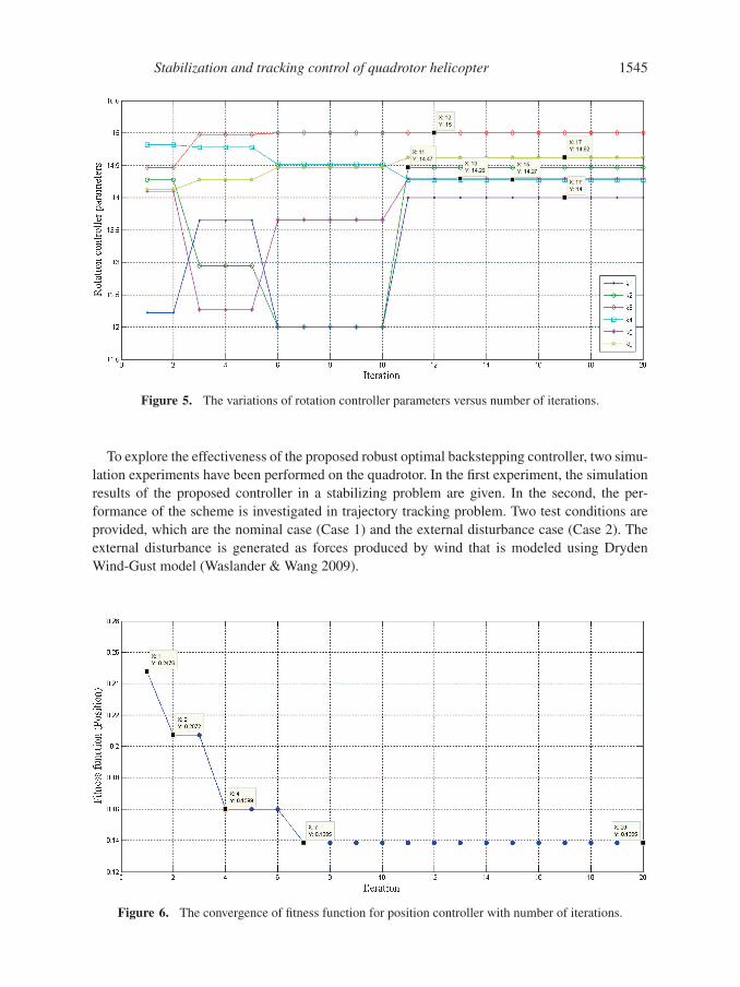
For the position controller, the best fitness value is 0.1385 appeared in iteration number 7, and

the optimal parameters are k7 = 15.00, k8 = 15.00, k9 = 14.29, k10 = 14.79, k11 = 14.70 and

k12 = 15.00. The variation of the fitness function with number of iterations is shown in figure 6.

Meanwhile, the variations of backstepping control parameters with respect to the number of

iterations are shown in figure 7. As can be seen for both control parameters optimization, through

about 20 iterations, the GSA method can prompt convergence and obtain good fitness value.

Figure 4. The convergence of fitness function for rotation controller with number of iterations.


Figure 5. The variations of rotation controller parameters versus number of iterations.

To explore the effectiveness of the proposed robust optimal backstepping controller, two simu-

lation experiments have been performed on the quadrotor. In the first experiment, the simulation

results of the proposed controller in a stabilizing problem are given. In the second, the per-

formance of the scheme is investigated in trajectory tracking problem. Two test conditions are

provided, which are the nominal case (Case 1) and the external disturbance case (Case 2). The

external disturbance is generated as forces produced by wind that is modeled using Dryden

Wind-Gust model (Waslander & Wang 2009).

Figure 6. The convergence of fitness function for position controller with number of iterations.


Figure 7. The variations of position controller parameters versus number of iterations.

6.1 Simulation experiment 1: stabilizing problem

In this simulation experiment, the control objective is to regulate a quadrotor at a certain desired

altitude/attitude, such that the quadrotor can hover at a fixed point. The desired altitude/attitude is

given by xid = [zd , φd , θd , ψd ] = [5, 0, 0, 0]T . The initial states are given by z = 5, φ = 0.2,

0 2 4 6 8 104.8

4.9

5

5.1

Z position

z [

m]

Time [s]

0 2 4 6 8 10-0.1

0

0.1

0.2Roll angle

Ro

ll [

rad

]

Time [s]

0 2 4 6 8 10-0.1

0

0.1

0.2Pitch angle

Pit

ch

[ra

d]

Time [s]

0 2 4 6 8 10-0.1

0

0.1

0.2Yaw angle

Yaw

[ra

d]

Time [s]

Desired

Output

Figure 8. Altitude/attitude stabilization of the hovering quadrotor using OBC at Case 1.


0 2 4 6 8 104.8

4.9

5

5.1

5.2Z position

z [

m]

Time [s]

0 2 4 6 8 10-0.1

0

0.1

0.2Roll angle

Ro

ll [

rad

]

Time [s]

0 2 4 6 8 10-0.1

0

0.1

0.2Pitch angle

Pit

ch

[ra

d]

Time [s]

0 2 4 6 8 10-0.1

0

0.1

0.2Yaw angle

Yaw

[ra

d]

Time [s]

Desired

Output

Figure 9. Altitude/attitude stabilization of the hovering quadrotor using OBC at Case 2.

0 2 4 6 8 104.8

4.9

5

5.1

5.2Z position

z [

m]

Time [s]

0 2 4 6 8 10-0.1

0

0.1

0.2Roll angle

Ro

ll [

rad

]

Time [s]

0 2 4 6 8 10-0.1

0

0.1

0.2Pitch angle

Pit

ch

[ra

d]

Time [s]

0 2 4 6 8 10-0.1

0

0.1

0.2Yaw angle

Yaw

[ra

d]

Time [s]

Desired

Output

Figure 10. Altitude/attitude stabilization of the hovering quadrotor using ROBC at Case 1.


0 2 4 6 8 104.8

4.9

5

5.1

5.2Z position

z [

m]

Time [s]

0 2 4 6 8 10-0.1

0

0.1

0.2Roll angle

Ro

ll [

rad

]

Time [s]

0 2 4 6 8 10-0.1

0

0.1

0.2Pitch angle

Pit

ch

[ra

d]

Time [s]

0 2 4 6 8 10-0.1

0

0.1

0.2Yaw angle

Yaw

[ra

d]

Time [s]

Desired

Output

Figure 11. Altitude/attitude stabilization of the hovering quadrotor using ROBC at Case 2.

0 2 4 6 8 103

4

5

6

U1

[N

]

Time [s]

0 2 4 6 8 10-2

0

2

U2

[N

]

Time [s]

0 2 4 6 8 10-2

0

2

U3

[N

]

Time [s]

0 2 4 6 8 10-2

0

2

U4

[N

]

Time [s]

5 5.0002 5.0004 5.0006 5.0008 5.001-2

0

2

Figure 12. Control inputs of ROBC with sign function.


0 2 4 6 8 103

4

5

6

U1 [

N]

Time [s]

0 2 4 6 8 10-2

-1

0

1

2

U2 [

N]

Time [s]

0 2 4 6 8 10-2

-1

0

1

2

U3 [

N]

Time [s]

0 2 4 6 8 10-2

-1

0

1

2

U4 [

N]

Time [s]

5 5.0002 5.0004 5.0006 5.0008 5.001-2

0

2

Figure 13. Control inputs of ROBC with saturation function.

θ = 0.2 and ψ = 0.2. In the simulation, first, the OBC system is considered. The simulation

results of the OBC system for stabilizing a quadrotor at Case 1 and Case 2 are depicted in

figures 8 and 9, respectively. From the simulation results, the OBC system is able to stabilize

the quadrotor in hover mode at Case 1. However, the degenerate performance response shown

in figure 9 is resulted under the occurrence of external disturbance. Under the same simulation

cases, the ROBC system is simulated. The simulation results for stabilizing a quadrotor at Case

1 and Case 2 are depicted in figures 10 and 11, respectively. From the simulation results, the

robust control performance of the proposed ROBC system in the quadrotor stabilization can be

observed. It can be clearly seen that the altitude/attitude of the quadrotor can be maintained at

the desired altitude/attitude, that is, the hovering flight is stable even if the external disturbance

is exerted as shown in figure 11. As aforementioned, the using of sign switching function will

cause undesirable phenomenon called chatter in the control input as shown in figure 12. The

effective way to counter this problem is by utilizing the saturation function and the result can be

seen in figure 13.

6.2 Simulation experiment 2: trajectory tracking problem

In this simulation experiment, the control objective is to ensure the quadrotor can effectively

track the desired reference trajectory. The helical trajectory is adopted to test the trajectory


-1

0

1

2

3

-1

0

1

2

30

0.5

1

1.5

2

2.5

3

x(m)y(m)

z(m

)

Desired

Output

Wind

Wind

End position

Initial position

Figure 14. Helical trajectory tracking response using OBC at Case 2.

-1

0

1

2

3

-1

0

1

2

3

0

0.5

1

1.5

2

2.5

3

x(m)y(m)

z(m

)

Desired

Output

Wind

Wind

End position

Initial position

Figure 15. Helical trajectory tracking response using ROBC at Case 2.


tracking capability of the quadrotor by the OBC and ROBC system. The desired trajectory is

generated using the following command:

⎧

⎨

⎩

xd = sin (t) ,

yd = cos (t) ,

zd = 1 + 0.2t.

(60)

The initial state of the quadrotor is set to be [x0, y0, z0] = [1, 1, 0]m. The simulation results of

helical trajectory tracking for both OBC and ROBC approaches under the occurrence of external

disturbance are respectively shown in figures 14 and 15. As it can be seen, the proposed control

scheme can track the desired reference trajectory accurately despite external disturbance. It is

obvious that the ROBC can give small tracking error and good tracking performance compared

to OBC.

7. Conclusions

In this paper, the application of a robust controller for stabilization and trajectory tracking of

a quadrotor helicopter perturbed by external disturbances is successfully demonstrated. First,

the mathematical model of the quadrotor is introduced. Then, the proposed robust control

system, which comprises a backstepping and a switching function, is developed. The backstep-

ping control design is derived based on Lyapunov function, so that the stability of the system

can be guaranteed, while switching function is used to attenuate the effects caused by distur-

bances. GSA has been utilized to determine the controller parameters. Finally, the proposed

control scheme is applied to autonomous quadrotor helicopter. Simulation results show that

high-precision transient and tracking response can be achieved by using the proposed control

system.

References

Baek S J, Lee D J, Park J H and Chong K T 2013 Design of lateral Fuzzy-PI controller for unmanned

quadrotor robot. J. Inst. Control, Robotics Syst. 19: 164–170

Bolandi H, Rezaei M, Mohsenipour R, Nemati H and Smailzadeh S 2013 Attitude control of a Quadrotor

with optimized PID controller. Intelligent Control Autom. 4: 335–342

Boškovic D M and Krstic M 2002 Backstepping control of chemical tubular reactors. Comp.Chem. Eng.

26: 1077–1085

Bouadi H, Bouchoucha M and Tadjine M 2007 Modelling and stabilizing control laws design based on

sliding mode for an UAV Type-Quadrotor. Eng. Lett. 15: 342–347

Bouadi H, Bouchoucha M and Tadjine M 2008 Sliding mode control based on backstepping approach for

an UAV type-quadrotor. Int. J. Appl. Math. Comp. Sci. 4: 12–17

Castillo P, Lozano R and Dzul A 2005 Stabilization of a mini rotorcraft with four rotors. IEEE Control

Syst. Mag. 25: 45–55

Chiu C H, Peng Y F and Lin Y W 2011 Intelligent backstepping control for wheeled inverted pendu-

lum. Expert Syst. Appl. 38: 3364–3371

De Moura Oliveira P, Pires E S and Novais P 2013 Gravitational search algorithm design of Posicast PID

control systems. Soft Computing Models in Industrial and Environmental Applications (pp. 191–199):

Springer

Erginer B and Altug E 2012 Design and implementation of a hybrid fuzzy logic controller for a quadrotor

VTOL vehicle. Int. J. Control, Autom. Syst. 10: 61–70


Guisser M H and Medromi H 2009 A high gain observer and sliding mode controller for an autonomous

quadrotor helicopter. Int. J. Intell. Control Syst. 14: 204–212

Hu Q, Xu L and Zhang A 2012 Adaptive backstepping trajectory tracking control of robot manipulator. J.

Franklin Inst. 349: 1087–1105

Hwang J H, Hwang S, Hong S K and Yoo M G 2012 Attitude stabilization performance improvement of

the quadrotor flying robot. J. Inst. Control Robot. Syst. 18: 608–611

Jafari H, Zareh M, Roshanian J and Nikkhah A 2010 An optimal guidance law applied to quadrotor using

LQR method. Trans. Japan Soc. Aeronaut. Space Sci. 53: 32–39

Jiang Y, Hu Q and Ma G 2010 Adaptive backstepping fault-tolerant control for flexible spacecraft with

unknown bounded disturbances and actuator failures. ISA Trans. 49: 57–69

Junior J C V, De Paula J C, Leandro G V and Bonfim M C 2013 Stability control of a quad-rotor using a

PID controller. Brazilian J. Instrum. Control 1: 15–20

Kim H M, Park S H, Song J H and Kim J S 2010 Robust position control of electro-hydraulic actuator

systems using the adaptive back-stepping control scheme. Proc. Inst. Mech. Eng. I: J. Syst. Control Eng.

224: 737–746

Kristiansen R, Nicklasson P J and Gravdahl J T 2009 Satellite attitude control by quaternion-based

backstepping. IEEE Trans. Control Syst. Technol. 17: 227–232

Krstic M, Kanellakopoulos I and Kokotovic P 1995 Nonlinear and adaptive control design, (Vol. 222):

Wiley New York

Lee D, Ha C and Zuo Z 2013 Backstepping control of quadrotor-type UAVs and its application to teleop-

eration over the Internet. 12th International Conference on Intelligent Autonomous Systems, Jeju Island,

vol. 194, pp. 217–225

Madani T and Benallegue A 2006 Backstepping control for a quadrotor helicopter. IEEE/RSJ International

Conference on Intelligent Robots and Systems, pp. 3255–3260

Mokhtari A, M’Sirdi N K, Meghriche K and Belaidi A 2006 Feedback linearization and linear observer for

a quadrotor unmanned aerial vehicle. Adv. Robot. 20: 71–91

Mukherjee P and Waslander S L 2012 Direct adaptive feedback linearization for quadrotor control. AIAA

Guidance, Navigation, and Control Conference

Nuchkrua T and Parnichkun M 2012 Identification and optimal control of Quadrotor. Thammasat Int. J.

Sci. Technol. 17: 36

Olfati-Saber R 2000 Nonlinear control of underactuated mechanical systems with application to robotics

and aerospace vehicle. Ph.D. thesis, Massachusetts Institute of Technology

Rashedi E, Nezamabadi-Pour H and Saryazdi S 2009 GSA: a gravitational search algorithm. Information

Sci. 179: 2232–2248

Regula G and Lantos B 2011 Backstepping based control design with state estimation and path tracking to

an indoor quadrotor helicopter. Electr. Eng. Comput. Sci. 53: 151–161

Santos M, López V and Morata F 2010 Intelligent fuzzy controller of a quadrotor. IEEE International

Conference on Intelligent Systems and Knowledge Engineering, pp. 141–146

Shen Q, Jiang B and Cocquempot V 2013 Adaptive fault-tolerant backstepping control against actuator gain

faults and its applications to an aircraft longitudinal motion dynamics. Int. J. Robust Nonlinear Control

23: 1753–1779

Sumantri B, Uchiyama N, Sano S and Kawabata Y 2013 Robust tracking control of a quad-rotor. Helicopter

utilizing sliding mode control with a nonlinear sliding surface. J. Syst. Des. Dyn. 7: 226–241

Sun W, Gao H and Kaynak O 2013 Adaptive backstepping control for active suspension systems with hard

constraints. IEEE/ASME Trans. Mechatronics 18: 1072–1079

Voos H 2009 Nonlinear control of a quadrotor micro-UAV using feedback-linearization. IEEE International

Conference on Mechatronics, pp. 1–6

Waslander S L and Wang C 2009 Wind disturbance estimation and rejection for quadrotor position control.

AIAA Infotech@ Aerospace Conference and AIAA Unmanned... Unlimited Conference, Seattle, WA

Xu J X, Guo Z Q and Lee T H 2012 Synthesized design of a fuzzy logic controller for an underactuated

unicycle. Fuzzy Sets Syst. 207: 77–93


Yang J H and Yang K S 2012 An adaptive variable structure control scheme for underactuated mechanical

manipulators. Math. Problems Eng. 2012

Yih C C 2013 Sliding mode control for swing-up and stabilization of the cart-pole underactuated

system. Asian J. Control 15: 1201–1214

Yu R, Zhu Q, Xia G and Liu Z 2012 Sliding mode tracking control of an underactuated surface vessel. IET

Control Theory Appl. 6: 461–466

Zhang Y, Zhao W, Lu T and Li J 2013 The attitude control of the four-rotor unmanned helicopter based on

feedback linearization control. WSEAS Trans. Syst. 12: 229–239

Zilic T, Kasac J, Situm Z and Essert M 2013 Simultaneous stabilization and trajectory tracking of

underactuated mechanical systems with included actuators dynamics. Multibody Syst. Dyn. 29: 1–19

stabilization and trajectory tracking control for

Documents