cyclist detection, tracking, and trajectory analysis in
TRANSCRIPT
UNLV Theses, Dissertations, Professional Papers, and Capstones
August 2017
Cyclist Detection, Tracking, and TrajectoryAnalysis in Urban Traffic Video DataFarideh Foroozandeh ShahrakiUniversity of Nevada, Las Vegas, [email protected]
Follow this and additional works at: https://digitalscholarship.unlv.edu/thesesdissertations
Part of the Computer Engineering Commons, and the Electrical and Computer EngineeringCommons
This Thesis is brought to you for free and open access by Digital Scholarship@UNLV. It has been accepted for inclusion in UNLV Theses, Dissertations,Professional Papers, and Capstones by an authorized administrator of Digital Scholarship@UNLV. For more information, please [email protected].
Repository CitationForoozandeh Shahraki, Farideh, "Cyclist Detection, Tracking, and Trajectory Analysis in Urban Traffic Video Data" (2017). UNLVTheses, Dissertations, Professional Papers, and Capstones. 3077.https://digitalscholarship.unlv.edu/thesesdissertations/3077

CYCLIST DETECTION, TRACKING, AND TRAJECTORY ANALYSIS
IN URBAN TRAFFIC VIDEO DATA
By
Farideh Foroozandeh Shahraki
Bachelor of Science- Computer Engineering
Isfahan University of Technology, Iran
2013
A thesis submitted in partial fulfillment
of the requirements for the
Master of Science - Electrical Engineering
Department of Electrical and Computer Engineering
Howard R. Hughes College of Engineering The
Graduate College
University of Nevada, Las Vegas
August 2017

Copyright 2017 by Farideh Foroozandeh Shahraki
All Rights Reserved
ii
Thesis Approval
The Graduate College
The University of Nevada, Las Vegas
June 9, 2017
This thesis prepared by
Farideh Foroozandeh Shahraki
entitled
Cyclist Detection, Tracking, and Trajectory Analysis in Urban Traffic Video Data
is approved in partial fulfillment of the requirements for the degree of
Kathryn Hausbeck Korgan, Ph.D. Graduate College Interim Dean
Master of Science - Electrical Engineering
Department of Electrical and Computer Engineering
Emma Regentova, Ph.D. Examination Committee Chair
Venkatesan Muthukumar, Ph.D. Examination Committee Member
Brendan Morris, Ph.D. Examination Committee Member
Pramen Shrestha , Ph.D. Graduate College Faculty Representative

iii
ABSTRACT
The major objective of this thesis work is examining computer vision and machine
learning detection methods, tracking algorithms and trajectory analysis for cyclists in traffic
video data and developing an efficient system for cyclist counting. Due to the growing number of
cyclist accidents on urban roads, methods for collecting information on cyclists are of significant
importance to the Department of Transportation. The collected information provides insights into
solving critical problems related to transportation planning, implementing safety
countermeasures, and managing traffic flow efficiently. Intelligent Transportation System (ITS)
employs automated tools to collect traffic information from traffic video data. In comparison to
other road users, such as cars and pedestrians, the automated cyclist data collection is relatively a
new research area. In this work, a vision-based method for gathering cyclist count data at
intersections and road segments is developed. First, we develop methodology for an efficient
detection and tracking of cyclists. The combination of classification features along with motion
based properties are evaluated to detect cyclists in the test video data. A Convolutional Neural
Network (CNN) based detector called You Only Look Once (YOLO) is implemented to increase
the detection accuracy. In the next step, the detection results are fed into a tracker which is
implemented based on the Kernelized Correlation Filters (KCF) which in cooperation with the
bipartite graph matching algorithm allows to track multiple cyclists, concurrently. Then, a
trajectory rebuilding method and a trajectory comparison model are applied to refine the
accuracy of tracking and counting. The trajectory comparison is performed based on semantic
similarity approach. The proposed counting method is the first cyclist counting method that has
the ability to count cyclists under different movement patterns. The trajectory data obtained can
be further utilized for cyclist behavioral modeling and safety analysis.

iv
ACKNOWLEDGMENTS
I would like to express my profound gratitude to my academic advisor, Dr. Emma
Regentova, for her scholastic advice and technical guidance throughout this investigation. Her
devotion, patience, and focus on excellence allowed me to reach this important milestone in my
life. I also wish to extend my acknowledgements to the examination committee members, Dr.
Venkatesan Muthukumar, Dr. Brendan Morris, and Dr. Pramen Shrestha for their guidance and
suggestions.
I wish to thank Mr. Ali Pour Yazdanpanah for providing unlimited assistance and support
during my study.

v
DEDICATION
This study is dedicated to my husband, Ebrahim, and my parents, Fereshteh and
Daryoosh. Without their continued and unconditional love and support, I would not be the person
I am today.

vi
TABLE OF CONTENTS
ABSTRACT ............................................................................................................................... iii
ACKNOWLEDGMENTS .......................................................................................................... iv
LIST OF TABLES ..................................................................................................................... ix
LIST OF FIGURES ..................................................................................................................... x
CHAPTER 1- INTRODUCTION ........................................................................................... 1
1.1. Motivation ........................................................................................................................ 3
1.2. Objectives ......................................................................................................................... 4
1.3. Overview .......................................................................................................................... 5
CHAPTER 2- LITERATURE REVIEW ................................................................................ 7
2.1. Detection .......................................................................................................................... 7
2.1.1. Appearance based approach ...................................................................................... 7
2.1.2. Motion based approach ............................................................................................. 9
2.1.3. Convolutional Neural Network approach ............................................................... 10
2.2. Tracking ......................................................................................................................... 12
2.3. Counting ......................................................................................................................... 14
CHAPTER 3- SYSTEM OVERVIEW ................................................................................. 18
CHAPTER 4- DATASETS ................................................................................................... 20
4.1. Training dataset .............................................................................................................. 20
4.2. Test dataset ..................................................................................................................... 22
CHAPTER 5- CYCLIST DETECTION ............................................................................... 24
vii
5.1. Histogram of Oriented Gradient (HOG) Feature ........................................................... 24
5.2. Multi-scale Local Binary pattern (MLBP) Feature ........................................................ 25
5.3. Histogram of Shearlet Coefficients (HSC) Feature ........................................................ 27
5.4. Background subtraction: Gaussian Mixture Model (GMM) .......................................... 29
5.5. Combined Feature .......................................................................................................... 31
5.6. Support Vector Machine (SVM) Classification ............................................................. 32
5.7. Convolutional Neural Network (CNN) .......................................................................... 33
5.7.1. Components of Convolutional Neural Network (CNN) ......................................... 36
5.7.2. You Only Look Once (YOLO) ............................................................................... 39
5.7.2.1. YOLOv1 .......................................................................................................... 39
5.7.2.2. YOLOv2 .......................................................................................................... 41
CHAPTER 6- CYCLIST TRACKING ................................................................................. 47
6.1. Kernelized Correlation Filter (KCF) Tracking ............................................................... 48
6.2. Multiple Object Tracking ............................................................................................... 53
CHAPTER 7- CYCLIST COUNTING ................................................................................. 57
7.1. Trajectory Rebuilding .................................................................................................... 58
7.2. POI model ...................................................................................................................... 60
CHAPTER 8- EXPERIMENTS AND RESULTS ................................................................ 64
8.1. Performance of Classification ........................................................................................ 65
8.2. Performance of Detection ............................................................................................... 65
8.3. Performance of Tracking ................................................................................................ 68
8.4. Performance of Counting ............................................................................................... 71

viii
CHAPTER 9- CONCLUSION AND FUTURE WORK ...................................................... 73
9.1. Summary of work ........................................................................................................... 73
9.2. Future work .................................................................................................................... 73
REFERENCES ............................................................................................................................. 75
CURRICULUM VITAE ............................................................................................................... 82

ix
LIST OF TABLES
Table 4.1 Training Dataset ............................................................................................................ 22
Table 5.1 YOLOv2 Configuration ................................................................................................ 46
Table 8.1 Area Under ROC Curve (AUC) for each feature ......................................................... 65
Table 8.2 Detection result ............................................................................................................. 66
Table 8.3 The tracking result ........................................................................................................ 69
Table 8.4 Number of broken segments for each path direction .................................................... 69
Table 8.5 Counting result (before/after) trajectory rebuilding ...................................................... 71

x
LIST OF FIGURES
Figure 3.1 System flowchart ......................................................................................................... 19
Figure 4.1 Cyclist different orientation views .............................................................................. 20
Figure 4.2 (a) Sample images from dataset type A, (b) Sample images from dataset type B ...... 21
Figure 4.3 Camera setting at the intersection................................................................................ 23
Figure 4.4 Positive image samples of the test video data ............................................................. 23
Figure 5.1 Visualization of HOG feature of a cyclist ................................................................... 25
Figure 5.2 Pixels marked for three-scale MLBP with radii 1,3, and 5, in 8 orientations ............. 27
Figure 5.3 Extraction Feature for a decomposition in 2 levels and 8 orientations for each level.
courtesy of (Schwartz et al. 2011) ................................................................................................ 29
Figure 5.4 Moving regions (Blue), the green and red regions show intersection and road segment,
respectively. .................................................................................................................................. 30
Figure 5.5 Detection pipeline for combined feature detector ....................................................... 32
Figure 5.6 A simple example of fully connected layer feed forward neural network with two
hidden layers ................................................................................................................................. 35
Figure 5.7 YOLO Loss function ................................................................................................... 41
Figure 6.1 Tracking in cases with occlusions - (1) partial occlusion, (2) full occlusion .............. 53
Figure 6.2 Cyclist tracking system flowchart ............................................................................... 56
Figure 7.1 Cyclist’s trajectories of “sufficient” lengths................................................................ 59
Figure 7.2 Paths of Interest (POIs) ............................................................................................... 63
Figure 8.1 Detection examples by (1) pre-trained YOLOv2, (2) YOLOv2 trained from scratch,
(3) Combined GMM-HOG-MLBP ............................................................................................... 67

xi
Figure 8.2 Detection examples by (1) pre-trained YOLOv2, (2) YOLOv2 trained from scratch,
(3) Combined GMM-HOG-MLBP ............................................................................................... 68
Figure 8.3 Tracking examples, the distance between centroids is based on the cyclist’s velocity
and the distance between cyclist and the camera. ......................................................................... 70
Figure 8.4 Examples of trajectory rebuilding (to be viewed in color) .......................................... 72

1
CHAPTER 1- INTRODUCTION
The number of general traffic accidents is currently decreasing because of efficient
transportation safety measures by Department of Transportation (DOT) that makes use of data
and methods of Intelligent Transportation Systems. Vehicle and pedestrian detection attracted
lots of attention in the course of improving transportation safety. In recent, the safety of cyclists
is of a greatest concern because cyclist accidents are gradually increasing in numbers. According
to the literature (NHTSA 2014), cyclists are vulnerable on the roads and intersections. One of the
main factors in evaluating the risks is accurate vehicle, pedestrian and cyclist counts and
determination of their absolute and relative paths. Counting methods can be automated or
manual. Manual counts can be done directly in the field or by the visual analysis of traffic video
data. Automatic counting methods include computer vision techniques on video data. Although,
there exist numerous methodologies for automatic counting of vehicles and pedestrian, a lesser
research has been carried out for the automatic counting at intersections and roadway sections.
The DOT uses cameras in various locations of interest and a great amount of video data is
produced for the analysis that demands intensive cyclist detection, tracking and counting
methods for video based systems. Development of efficient methods of automated detection,
tracking, and counting is of great significance to the research and applications of Intelligent
Transportation Systems (ITS). The analysis of existing video recordings delivers the valuable
information about the nature of the problem, i.e., behavior, road and traffic conditions, so
conclusions can be drawn and safety measures can be developed. Furthermore, cyclist counts are
necessary to estimate cyclist activities (Zangenehpour et al. 2015). The Active Living Research
on cyclist counting technologies and the state of cycling research group (Ryan et al. 2013)
mentioned that some governments consider cyclist count data for allocating funds for certain

2
parks and evaluating potential projects. Cyclist count is usually done in off-line mode, where
high accuracy than a low computation cost is demanded. Despite the noticeable progress in
computer vision methods, the detection of cyclists is a challenging and open problem. Factors
contributing to the complexity of the problem include appearance similarity of the upper body of
a pedestrian and a cyclist that may lead to misdetection and subsequently to the wrong count in
the real road environment. Other factors include variety of poses in the field of view depending
on the camera location, illumination changes under day/night and environmental changes, and
occlusion of the target objects. The lack of a sufficient image resolution can cause misdetections
and may lead to failure of tracking. However, machine learning methods based on feature
extraction and classification have achieved a high performance over the span of last decade. In
this work, we demonstrate and evaluate an automatic video-based method for counting cyclists at
intersections and road sections. This method is implemented in three phases: detection, tracking,
and trajectory-based counting. We utilize both motion-based and appearance-based detection
approaches to design a fast and robust cyclist detection method. We use a combination of several
features which enhance the final combined feature performance. As the distance from the camera
to the image pane varies and object orientation changes, image features must be able to capture
details at different directions and scales. Deep learning techniques, especially convolutional
neural networks have shown significant improvement in object detection and recognition
accuracies. In this work, we also examine convolutional neural network approach for cyclist
detection. The Kalman Filter (KF) based (Chan et al. 1979) tracking performs relatively well for
cyclist and pedestrian tracking in traffic video data, but it is not robust under sudden changes in
cyclist movements, occlusion, and at low resolutions video frames. We elect a correlation based
tracker which performs well under the above conditions. In this work, we demonstrate and

3
evaluate an automatic vision based method for detecting, tracking, and counting cyclists in video
data taken at intersections and road sections.
1.1. Motivation
In transportation management, planning, and road safety, collecting data for both
motorized and non-motorized traffic is necessary (Robert 2009). Pedestrian, cyclist, and vehicle
safety is one of the most important transportation concerns in the world that makes intersections
and road segments an interesting target for monitoring. Although, there exist numerous
methodologies for monitoring of vehicles and pedestrian, a lesser research has been carried out
for data collecting and monitoring of cyclist at intersections and roadway sections (Foroozandeh
Shahraki et al. 2015). Bicycle usage has reported some positive trends in many urban areas in
North America. As the rate of bicycling as a mode of transportation has grown in United States,
concerns for bicyclist safety are also increasing and have become a critical issue for many cities
(Pucher et al. 2011). According to traffic safety facts published by US department of
transportation (NHTSA 2014), over the 10 years from 2005 to 2014, cyclist fatalities in traffic
crashes represented 1.8-2.2% of all road fatalities. While these numbers may not seem very high,
cyclist numbers continue to rise, so cyclist safety is becoming a major concern. Furthermore,
according to past research, it was found that the risk of injury for a person traveling through an
intersection as a cyclist is 14 times higher than an individual traveling in a vehicle (Strauss et al.
2014). Besides safety, behavior analysis of cyclist is useful for intersection and bicycle lane
design, estimate bicyclist activity such as bicycle ridership and infrastructure needs
(Zangenehpour et al. 2015). One of the main challenges in conducting detailed analysis on
cyclists’ behavior is the lack of reliable data.
4
Vision-based traffic scene perception (TSP) is one of many fast-emerging areas in the
intelligent transportation system (ITS) (Sivaraman et al. 2013). Traffic scene perception (TSP)
aims to extract accurate on-road environment data. Automatic information extraction involves
three phases: detection of objects of interest, tracking of objects in motion, and extract object
trajectory. Since trajectory extraction relies on the result of object tracking, and tracking often
depends on the results from detection, the ability to detect targets and track them effectively
plays a crucial role in TSP.
1.2. Objectives
In recent years, the protection of vulnerable road users, mainly pedestrians and cyclists,
has become one of the significant importance of department of transportation (Gandhi et al.
2007). And for this, vision based system of detection and tracking systems have broadly been
applied in traffic monitoring applications. But, the technical levels to protect both groups are
unbalance. Most of the vision based detection and tracking systems have been proposed for
pedestrian, whereas the detection systems for cyclist are mostly radar, infrared and acoustics
based (Dharmaraju et al. 2001).
The general objective of this thesis work is to evaluate a set of computer vision and
machine learning techniques to develop a system for efficient detection, tracking, and collecting
trajectory information of cyclists in urban traffic for collecting information on the number of
cyclists in different movement patterns.

5
1.3. Overview
In Chapter 1, a brief introduction to the research is presented, and the motivation and
objectives of the thesis are provided.
In Chapter 2, we review pertinent literature for vision-based object detection and
tracking. We also discuss existing vision-based approaches used for object counting.
In Chapter 3, we present an overview of our approach in cyclist monitoring system. We
provide a system flowchart of the developed system.
In Chapter 4, we describe the training and the test dataset used in the work.
In Chapter 5, we discuss the appearance based, motion based, their combination, and
convolutional neural network detection approaches which are applied to address the problem of
cyclist detection.
In Chapter 6, we describe the multi-object tracking methodology which is implemented
based on a correlation filter tracking and bipartite graph matching algorithm. We also talk about
the methodology which is used to solve the assignment problem between detected objects and
tracks, and handle miss detections and false detections.
In Chapter 7, we explain how incomplete trajectories are reconstructed using trajectory
rebuilding method. We also provide information of the counting methodology which apply
resultant complete trajectories to count cyclists in different movement direction.
In Chapter 8, the experimental results of detection, tracking, counting methods are
provided.

6
In Chapter 9, we summarize our work, and discuss the future work in this research area.

7
CHAPTER 2- LITERATURE REVIEW
2.1. Detection
In recent years, many methods have been proposed for detecting moving and motionless
objects. For detecting road users, different approaches based on different sensors have been
employed, and that includes monocular and stereo camera, lidar and radar. For pedestrian and
cyclist detection, vision sensors are preferred because of their capability to capture a high-
resolution perspective view of the scene with the useful color and texture information (Geronimo
et al. 2010). Furthermore, vision based techniques are more cost-effective than other methods
and can handle many other tasks, such as lane detection and traffic sign detection.
Vision based object detection methods are categorized to three major classes: detection
based on motion, detection based on appearance features, and convolutional neural network
(CNN) based detection.
2.1.1. Appearance based approach
In appearance based approach of object detection, selecting the correct feature is
important because overall performance of the system relies on the power of selected features
applied in detection method. There are three types of feature which have been mostly applied for
cyclist detection: a) single template features such as Haar (Viola et al. 2001), or features that are
histogram based like HOG (Dalal et al. 2005), LBP (Wang et al. 1990), and SIFT (Lowe 2004),
b) part based features such as deformable part-based model (DPM) (Felzenszwalb et al. 2010),
and c) geometric features. In geometric feature learning, the main goal is to find a set of
representative features of geometric form to represent an object by collecting geometric features

8
from images and learning them using efficient machine learning methods. All the feature types
use appearance properties of target such as shape, intensity, and texture.
H. Cho et al. (2010) suggested a Deformable Part-based Model (DPM) for bicycle
detection. In this method, a Principal Component Analysis (PCA) version of HOG and Linear
Support Vector Machine (SVM) were applied. Also, this method used Extended Kalman Filter
(EKF) based tracker method. Jung et al. (2012) proposed a method based on the improved HOG
feature which was named Multiple-Size Cell HOG (MSC-HOG) and Real-Adaboost (Schapire et
al. 1999) to detect bicycle. Dahiya et al. (2016) proposed an approach for detecting bicyclist
without helmet. This method used both motion based and appearance based approaches of
detection. First, an improved adaptive Gaussian Mixture Model (GMM) (Zivkovic 2004) was
applied to distinguish between moving and static objects in video frames. Then, three features,
i.e., HOG, LBP and SIFT were separately used to classify the moving object returned by
background subtraction that is bicyclist or another present object. The performance of these three
features were compared. Lin et al. (2017) proposed a side-view bicycle detection method based
on the geometric relationship of two wheels and two triangles in the side-view of bicycle images.
In this method, Triangle and elliptic shapes are used because they remain still triangle and ellipse
after prospective projection. This method applies an adaptive Canny edge detector, and the edge
information is classified to detect triangles and ellipses using Hough transform. Based on the
geometric relationship between detected triangles and ellipses, bicycle frames and two pairs of
wheels are found, and then a geometric model validation is applied to connect all the parts of
bicycle. This method is not appropriate for bicycle detection in the traffic video because it is not
rotation invariant and is not robust under noisy or small images of bicycles. Another geometry
based bicycle detection proposed by Fujimoto et al. (2013). This work is a combination of

9
motion based and appearance based detection methods. First, an optical flow algorithm is used to
find moving regions of video frames. Then, the ellipse approximation is applied to estimate the
tire of bicycle in the moving regions. This method also evaluates the width of the tire to estimate
the tire angle. Therefore, this work is useful to estimate the traffic direction of a bicycle. But, it
does not work properly in the presence of occlusion.
2.1.2. Motion based approach
The detection of moving objects is utilized in many applications such as object
classification, personal identification, object tracking and activity analysis. Hu et al. (2004)
categorized motion detection methods into three main classes: frame differencing, background
subtraction and Gaussian mixture model which is an adaptive background subtraction. Frame
differencing is a pixel-wise differencing between two or three consecutive frames in an image
sequence to detect regions corresponding to moving object. The idea in background subtraction
(Sugandi et al. 2007) is subtract the current image from a reference background image, which is
updated over time. It works well only in the presence of stationary cameras without any
illumination changes. GMM is an adaptive background subtraction method used for detecting
moving objects in video frames. Gaussian mixtures are used to model each pixel in the frame.
Moving regions are detected in a group of pixels whose distribution does not fit the Gaussian
distribution of the background pixels. GMM efficiently handles illumination changes, slow and
repetitive motion. Motion based detection methods mostly are used in real time applications
because they are faster than appearance based detection methods. Li et al. (2009) proposed a real
time pedestrian detection based on GMM. In some cases, the motion based and appearance based
approaches are used in combination to speed up and augment the detection. For instance,

10
Fujimoto et al. (2013) and Dahiya et. al (2016) have applied motion based detection before using
the appearance features.
2.1.3. Convolutional Neural Network approach
Substantial amounts of training data and increased computing power have led to recent
successes of deep architectures (typically convolutional neural networks) for object
classification. Some methods have gone one step further and addressed the problem of object
detection and object recognition. Most of appearance based detection systems repurpose
classifiers to perform detection. To detect an object, these systems take a classifier for that object
and evaluate it at various scales and locations in a test image. Systems like HOG and SVM and
DPM use a sliding window approach where the classifier is run at evenly spaced locations over
the entire image. But CNNs detection models work differently. For instance, R-CNN (Girshick et
al. 2014) extract potential bounding boxes using region proposal methods such as Selective
Search (SS) and then classify these proposed bounding boxes with a CNN-based classifier. After
classification, post-processing is used to refine the bounding boxes, eliminate duplicate
detections, and rescore the boxes based on other objects in the scene. Despite the overall success
of R-CNN, training an R-CNN model is expensive in terms of memory and time usage. By
sharing computation of convolutional layers between region proposals for an image and
replacing Selective Search (SS) with a neural network which is called Region Proposal Network
(RPN), Fast R-CNN (Girshick 2015) and Faster R-CNN (Ren et al. 2015) are able to achieve
higher accuracies and better latencies overall. Instead of having a sequential pipeline of region
proposals and object classification, YOLO (Redmon et al. 2016a) method has formulated object
detection as a single regression problem, straight from image pixels to bounding box coordinates
11
and class probabilities. In this detection, a single convolutional network simultaneously predicts
multiple bounding boxes and class probabilities for those boxes. YOLO trains on full images and
directly optimizes detection performance. This leads a much lower latency.
CNNs are also used in pedestrian and cyclist detection. For instance, Li et al. (2016)
introduced a new method called Stereo-Proposal based Fast R-CNN (SP-FRCN) to detect
cyclists. Li et al. (2017) presented a unified framework for concurrent pedestrian and cyclist
detection, which includes a novel detection proposal method (termed UB-MPR) to output a set of
object candidates, a discriminative deep model based on Fast R-CNN for classification and
localization, and a specific postprocessing step to further improving the detection performance.
This method has taken advantages of the difference between pedestrian and rider of bicycle. It
means that to detect cyclist, only the rider part has been examined.
Although CNN based detection methods do not need manually selected features and a
classifier running all over the image, this approach requires large amount of data for training. To
overcome this challenge for problems which do not have sufficient training data, some methods
use transfer learning. Transfer learning is transferring learned features of a pre-trained network to
a new detection case. It is possible to fine-tune all the layers of the pre-trained network, or fix the
initial layers of the network which contain more generic features such as edge or color, and only
fine-tune the last few layers which are higher-level portion of the network to learn specific
features of the new dataset (typically a smaller dataset). Compare to training a new CNN,
transfer learning usually needs a lesser training time.

12
2.2. Tracking
Tracking is applied in numerous applications such as motion based detection and
recognition, automated surveillance, video indexing, traffic monitoring, vehicle navigation, and
medical image indexing. Many tracking methods have been proposed in literature for different
applications. These tracking methods are categorized to point tracking, kernel tracking, silhouette
tracking, or correlation filter tracking methods.
In point trackers, first a detector is applied to detect the objects in every frame. Then,
detected objects in consecutive frames are represented by points. The association of these points
is based on the previous object position and motion (Yilmaz et al. 2006). Point Tracking is a
difficult problem particularly in the existence of miss detections and partial and full occlusions.
Kalman-filter based tracking is a point tracking method which use statistical approach for point
correspondence. In statistical correspondence methods, state space approach is used to model
object properties such as velocity, acceleration, and location. Kalman filtering is composed of
two stages, prediction and correction (Banerjee et al. 2008). Prediction of the next state using the
current set of observations and update the current set of predicted measurements. The second
step gradually updates the predicted values and gives a much better approximation of the next
state. Banerjee et al. (2008) used Kalman filter for multi person tracking. In (Cho et al. 2010),
Kalman filter tracking is applied to estimate the velocity and the location of the bicycle in its
coordinates. One of the limitations of the Kalman filter is that it gives a poor estimation of state
variables which are not normally (Gaussian) distributed.
Kernel tracking refers to the object appearance and shape. In this method, the motion of
the kernel is computed in consecutive frames and the object is tracked. Kernel motion is in the
13
form of translation, rotation, or affine. Kernel based tracking algorithms differ by appearance
representation, computing motion, and the number of objects which are tracked. Cho et al.
(2010) proposed multiple patch-based Lucas-Kanade tracker to track bicyclist. In this method,
the Harris corner detector runs in bounding boxes returned by the detector. Then, each of these
multiple small patches are tracked independently using the Lucas-Kanade algorithm (J Shi
1994). The Lucas-Kanade tracker computes the suitable affine transformation for the features
found for a target in current frame to the features of the same target in next frame.
Silhouette tracking uses object region information to estimate object in the subsequent
frame. This region information can be density, edge information, or contour of the object. The
work in (Sato et al. 2004) proposed a shape matching using Hough transform which is used for
tracking purpose.
Such traditional algorithms almost have no considerations on target appearance model
variation, motion blur, articulated motions, abrupt motions, and illumination changes. Recently,
the algorithms based on correlation filter have proven their great strengths in efficiency and
robustness, and have considerably accelerated the development of visual object tracking (Chen et
al. 2015). Correlation Filter-based Tracking (CFT) is a tracking-by-detection method which is
discriminative approach. Discriminative tracking methods learn to distinguish the target from
backgrounds. In these methods, correlation filter gets the maximum response when it meets the
target. Henriques et al. (2015) proposed KCF tracker wherein detection is considered as a binary
kernel ridge regression problem. The multi-channel features and the approach to integrate them
together are applied in KCF to build an insensitive stronger classifier for illustration variation,

14
appearance model variation and motion blur. This method also takes advantage of circulant
matrix to speed up the tracking.
2.3. Counting
Automatic object (pedestrian, cyclist, vehicle, airplane, etc.) counting methods using
single camera are designed in the literature mostly upon three main approaches: a) counting in
the Region of Interest (ROI), b) counting across the Line of Interest (LOI), and c) counting using
trajectory analysis. In the ROI-based approach, the number of target objects is estimated in a
region of interest at a specific time interval. The LOI-based methods count a target object if it
passes through a line of interest. In contrast to ROI methods, LOI methods track the objects over
time to produce instantaneous total count. And, a trajectory based counting methods work based
on either the length of the gathered trajectory data or based on the comparison of the trajectory
data to some specific learned trajectories.
Chan et al. (2012) proposed the use of Bayesian Poisson regression to ROI-based count
of pedestrian crowds without using object detection or feature tracking. Li et al. (2011) presented
a crowd ROI-based counting in actual surveillance scenarios system using feature regression and
template matching. Ryan et al. (2009) introduced a ROI-based crowd counting applied group-
level tracking and local features to count the number of people in each group as represented by a
foreground blob segment; the tracking method analyzes the history of each group, including
splitting and merging events. Zhang et al. (2016) implemented a vehicle detection and ROI-
based counting for traffic surveillance videos based on Fast Region-based Convolution Network
(Fast R-CNN). This method counts the vehicles if they enter and exist a small road segment.
Zhou et al. (2016) proposed a real-time method to count people in crowded scenes using holistic

15
feature extraction and regression techniques in multiple ROIs, rather than by individual detection
and tracking. Cao et al. (2016) presented a simple bi-directional LOI based approach to count
pedestrians passing a gate with the use of background subtraction and by tracking extracted
blobs. This method considered two lines of interest to estimate left to right and right to left
directions. Cong et al. (2009) introduced a counting method by regarding the moving pedestrian
crowd as a fluid flow, and presented a novel crowd counting algorithm, which merged both LOI
and ROI approaches and applied the flow velocity field estimation model along with offline
learning. Yam et al. (2011) proposed a bi-directional LOI-based counting system incorporating
object detection and tracking to count the people flow in the monitored scene. This method
determined only two directions, i.e., bottom to top and top to bottom in video frames. Kocamaz
et al. (2016) presented a system of a cascaded detect-track-count procedures to count cyclists and
pedestrians if they cross a virtual LOI at intersections. Perng et al. (2016) represented an LOI
based people counting system using background subtraction and object tracking to count the
number of people are getting in/out of a bus. Wen et al. (2008) demonstrated a LOI-based
approach of counting system to count the number of people entering or leaving a building.
Barcellos et al. (2015) applied a LOI-based method of detecting and counting vehicles in urban
traffic videos using Gaussian Mixture Model (GMM) and particle filter based tracking. This
method defined a LOI and counted vehicles if they pass this line. Ma et al. (2016) presented a
novel crowd counting framework, which is based on integer programming to recover the
instantaneous counts on the LOI from Temporal ROI (TROI) counts. Zhao et. al (2016) proposed
a deep Convolutional Neural Network (CNN) for counting crowd across a line-of-interest (LOI)
in surveillance videos. In this method, CNN directly estimates the counts of pedestrians in a
crowd with pairs of video frames as inputs. The training has been performed with pixel-level

16
maps. Antonini et al. (2006) proposed a counting method of a crowd of pedestrians based on
trajectory clustering. This method clusters only the movements of crowd trajectories and does
not suite for individual counting. Shirazi et al. (2014) provided a trajectory-based counting
method for crossing and turning movement counts of vehicles at roadway segments. This method
compared the vehicle trajectories to certain learned trajectories without considering any
trajectory reconstruction. Because of errors of detection and tracking, some trajectories have
missing segments and cannot carry valuable information due to the short lengths of trajectories.
Zangenepour et al. (2015) proposed a trajectory-based counting method for counting cyclist flow
for various movements with different origins and destinations at intersection and road segment.
The limitation of this method is that it analyzes the cyclists on the straight trajectories at
intersections or bicycle lanes and thus cannot be extended to count cyclists who have turning
movements in street segments. Thus, it cannot be used for the safety analysis.
ROI-based counting methods are employed for counting for surveillance, urban planning
(e.g., identifying the crowd size around the area), and traffic management (e.g., control traffic
rate) purposes. They estimate the number of people and vehicles when they are in a specific
region, and for individual counts when the object enters and exits the ROI. However, the
approach in ROI methods is not to determine the movement direction of targets. So, they can be
useful for surveillance purposes but are not appropriate for safety measurements wherein the
directional information of targets is necessary. LOI-based counting methods are mostly applied
for identifying the flow rate of targets through a real gate or a virtual line which can be used for
resource management (e.g., counting the number of people entering and exiting a bus), traffic
management, surveillance, etc. LOI-based approach is used for estimating the number of
individuals or a crowd passing the line of interest. This approach lacks the information about the

17
direction for all target movements before and after passing the line. Thus, the same as the ROI-
based approach, the LOI-based approach cannot be applied for safety analysis. Trajectory based
counting methods are mostly used for individual flow counting. The major objective of the
trajectory-based methods is identifying different movements and directions of targets and their
paths that can be utilized in traffic management and road safety studies.

18
CHAPTER 3- SYSTEM OVERVIEW
In this chapter, we give an overview of how the various parts of the developed system
that are object detection, object tracking, trajectory rebuilding, and object counting are
associated. Figure 3.1 represents the flowchart of the automated cyclist detection and tracking in
RGB video data.
The first necessary component in vision based traffic monitoring is the dataset of traffic
video. In Chapter 4, we will discuss the available datasets which are used to develop and
evaluate our detector and the Nevada dataset that is collected by us in Las Vegas city for testing
the system. We will implement the Histogram of Oriented Gradient (HOG), Multi-scale Local
Binary Pattern (MLBP), Histogram of Shearlet Coefficients (HSC), the combination of HOG and
MLBP, and the combination of HOG and HSC. The combined feature is used in cooperation
with Gaussian Mixture Model (GMM) to improve the detection accuracy and speed. Also, a
Convolutional Neural Network (CNN) based detector called YOLO is implemented for detection
purpose. Our tracking approach which is a Kernelized Correlation Filter based Multi-Object
Tracker (KCF MOT) needs a bounding box information from the detector. In our system, we
implement KCF MOT over the YOLO detector. In counting phase, we reconstruct the trajectory
information obtained by the detection and tracking methods using a trajectory rebuilding method.
Then, the complete trajectory information is used to derive the cyclist counts in different
directions.

19
Figure 3.1 System flowchart

20
CHAPTER 4- DATASETS
4.1. Training dataset
As it is shown in Figure 4.1, cyclists have a high intra-class variation in different views.
We have eight orientation views which are at 0, 45, 90, 135, 180, 225, 270, and 315 degrees with
respect to the vertical axis of the frontal view of the cyclist. We divided the cyclist samples into
two classes: 0 and 180 degrees which are different from other classes are called “vertical” and
the rest of orientations for which the wheels can be observed are combined to a class named
“horizontal”.
Figure 4.1 Cyclist different orientation views
Since, cyclists and pedestrians carry similar features and this may cause false detections,
we divided the training dataset into two categories: type A) Images which contain the rider and
bicycle, and type B) Images which contain either bicycle images or bicycle with rider legs
images. Some samples of both dataset types are shown in Figure 4.2.

21
Figure 4.2 (a) Sample images from dataset type A, (b) Sample images from dataset type B
The classifier training dataset contains horizontal and vertical views of bicycle images.
The dataset type A images were collected from Gavrila.net (Li et al. 2016) and some samples of
Nevada dataset. Dataset Type B were collected from VOC (Everingham et al. 2010), ImageNet
(Russakovsky et al. 2015), ObjectNet3D (Xiang et al. 2016), Cityscapes (Bileschi 2006), and
Nevada datasets. We train the classifier using both types of dataset to evaluate the classification
rate, and select a best based on the outcome for detection. The “negative” dataset contains 9200
images of pedestrians, vehicles, motorcycles, buildings, road signs, and other elements collected
from the above collections.
Table 4.1 shows the number of images of all the datasets which are used as training
samples.

22
Table 4.1 Training Dataset
Dataset-type Dataset Number of
Horizontal
samples
Number of
Vertical
samples
Type A Gavrila.net 4509 7077
Nevada 4047 304
Total
number
8556 7381
Type B
VOC 330 34
Nevada 4047 304
ImageNet 322 90
ObjectNet3D 564 87
Cityscapes 377 93
Total
number
5640 608
4.2. Test dataset
The dataset used for testing is a part of Nevada dataset which was collected from an
intersection in Las Vegas (Maryland Pkwy and University road) during a period of five days in
April 2016, from noon to 1 pm at a highest cyclist traffic and in cloudy and sunny days. An
average distance between the camera and the intersection is 134.5 ft. The camera was mounted
on the top of a building. Figure 4.3 shows the geometry of installation.

23
Figure 4.3 Camera setting at the intersection
The dataset contains total of 540000 frames. 17500 frames of this dataset which contain
cyclists were selected for developing and testing the system. 8300 frames of this dataset which
contain a large number of cyclists were annotated for the test purpose. The frame resolution in
this dataset is 2048×1024. Figure 4.4 presents some samples of positive cases from the recorded
test video data.
Figure 4.4 Positive image samples of the test video data

24
CHAPTER 5- CYCLIST DETECTION
To detect cyclists in the traffic video sequences, Histogram of Oriented Gradient (HOG),
Multi-Scale Local Binary Patterns (MLBP) (Cao et al. 2012), and Histogram of Shearlet
Coefficients (HSC) (Schwartz et al. 2011) were used as classification features, and the Gaussian
mixture model (GMM) was utilized to find potential regions of moving pedestrian, cyclists and
vehicles. We explored a new Convolutional Neural Network (CNN), i.e., YOLO for cyclist
detection. These methods are discussed in detail in the following subsections.
5.1. Histogram of Oriented Gradient (HOG) Feature
The histogram of oriented gradients (HOG) is a feature used for the purpose of object
recognition. Object recognition using HOG features and the Support Vector Machine (SVM) is
quite popular approach for vehicle and pedestrian detection. HOG feature counts occurrences of
gradient orientations in localized parts of image. For this feature extractor, the image is divided
into blocks and each block is divided into cells. In each cell, the histogram of gradients is
computed. Histograms of cells are concatenated and then normalized with L2-norm
normalization to form a feature vector. The authors of HOG use a 64 × 128 detection window for
scanning the images. Each window is divided into 16 × 16 pixels’ size blocks with 50 % overlap
and each block consists of 4 cells each of 8 × 8 pixels. Four histograms of four cells make a 1D
feature vector of length 3780. Overall, each detection window has 7 × 15 = 105 overlapped
blocks. Figure 5.1 represents the visualization of HOG feature of a cyclist.

25
Figure 5.1 Visualization of HOG feature of a cyclist
5.2. Multi-scale Local Binary pattern (MLBP) Feature
Local Binary Pattern (LBP) is an efficient texture descriptor (Wang et al. 1990). LBP is a
descriptor of a small dimension. LBP computation is simple, and the descriptor is robust in the
presence of monotonic gray-scale changes caused by illumination variation. LBP is defined as an
order set of binary comparisons of pixel intensities between the central pixel and its surrounding
pixels. As an example, in 3×3 neighborhood, each of the 8 surrounding pixels is compared to the
central pixel. If the surrounding pixel intensity is larger or equal to the intensity of central pixel,
it is denoted by value of 1, otherwise it is 0.
The value of the LBP code of a central pixel (xc,yc) is given by :
𝐿𝐵𝑃𝑃,𝑅(𝑥𝑐, 𝑦𝑐) = ∑ 𝑠(𝑔𝑝 − 𝑔𝑐) × 2𝑝𝑃−1
𝑝=0 Eq. 5.1
𝑆(𝑥) = { 1, 𝑖𝑓 𝑥 ≥ 0;0, 𝑜𝑡ℎ𝑒𝑟𝑤𝑖𝑠𝑒
Eq. 5.2
Where gc and gp are gray values of central pixel and surrounding pixel, respectively, and
S(x) is the sign function. P represents the number of sampling points on a circle of radius R. For
26
a given central pixel (xc,yc), the position of surrounding pixels (xp,yp) where p ϵ P is represented
by the following formula:
(𝑥𝑝, 𝑦𝑝) = (𝑥𝑐 + 𝑅𝑐𝑜𝑠 (2𝜋𝑝
𝑃) , 𝑦𝑐 + 𝑅𝑠𝑖𝑛 (
2𝜋𝑝
𝑃)) Eq. 5.3
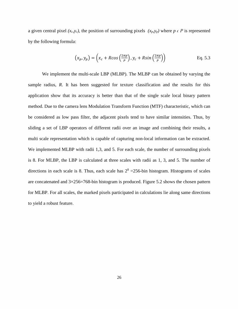
We implement the multi-scale LBP (MLBP). The MLBP can be obtained by varying the
sample radius, R. It has been suggested for texture classification and the results for this
application show that its accuracy is better than that of the single scale local binary pattern
method. Due to the camera lens Modulation Transform Function (MTF) characteristic, which can
be considered as low pass filter, the adjacent pixels tend to have similar intensities. Thus, by
sliding a set of LBP operators of different radii over an image and combining their results, a
multi scale representation which is capable of capturing non-local information can be extracted.
We implemented MLBP with radii 1,3, and 5. For each scale, the number of surrounding pixels
is 8. For MLBP, the LBP is calculated at three scales with radii as 1, 3, and 5. The number of
directions in each scale is 8. Thus, each scale has 28 =256-bin histogram. Histograms of scales
are concatenated and 3×256=768-bin histogram is produced. Figure 5.2 shows the chosen pattern
for MLBP. For all scales, the marked pixels participated in calculations lie along same directions
to yield a robust feature.

27
Figure 5.2 Pixels marked for three-scale MLBP with radii 1,3, and 5, in 8 orientations
5.3. Histogram of Shearlet Coefficients (HSC) Feature
Shearlet transform is a powerful tool for analyzing and representing data with anisotropic
information at multiple scales. Hence, signal singularities, such as edges, can be precisely
detected and located in images. To estimate the distribution of edge orientations, we use a feature
descriptor called Histograms of Shearlet Coefficients (HSC) which is an accurate multi-scale
analysis provided by shearlet transforms (Yi et al. 2009). HSC outperforms HOG for texture
classification and face identification.
The continuous shearlet transformation (Yi et al. 2009) of an image is defined as below.
SHφ(a, s, t) = ∫ f(x)ψa,s,t(t − x)dx Eq. 5.4
Where a, s, t are the scale, orientation, and location in spatial domain respectively and
𝑓(𝑥) is a two-dimensional image. Shearlets 𝜓𝑎,𝑠,𝑡 are given by

28
ψa,s,t(x) = |det Ka,s|−1
2 ψ(Ka,s−1 − t) Eq. 5.5
Ka,s = (a 𝑠√a
0 √a) = BA = (
a 00 √a
) (1 s0 1
) Eq. 5.6
Where A is an anisotropic scaling matrix and B is a shear matrix. 𝑓(𝑥) can be
reconstructed back using the following formula:
f = ∑ ⟨f, ψa,s,t⟩ψa,s,ta,s,t Eq. 5.7
Due to the good localization properties in both time and frequency of Meyer wavelet, this
wavelet is used as a mother wavelet for the implementation of the shearlet transform.
The HSC introduced in (Schwartz et al. 2011) uses statistics, i.e., a histogram of shearlet
coefficients instead of coefficients themselves for a compact representation. The HSC features
are calculated at different scales and orientations, since the shearlet coefficients are produced by
edges of different lengths and orientations (Easley et al. 2009). To calculate HSC features, the
image is divided into blocks. Each block is divided into 4 cells. In each cell, we perform
decomposition at levels and in a number of orientations. For each decomposition level, we
calculate the histogram with a number of bins equals the number of orientations in that
decomposition level. Entries of each bin are absolute values of the shearlet coefficients:
Hdl(s) = ∑ |SHφ(a, s, t)| Eq. 5.8
where Hdl(𝑠) is the s-th bin of the histogram for the dl-th decomposition level.
Finally, as it is shown in Figure 5.3, the histograms computed for all levels, cells and
blocks are concatenated and L2 normalization is employed. For implementation, we have used

29
8×8, 16×16, 32×32 and 64×64 blocks with 50% overlap to calculate HSC. Each block has four
cells. HSC feature is computed for each cell. We implement from 1 to 5 decompositions and 8
orientations per level. After testing, we have found that 8×8 blocks with 50% overlap and 4 cells
in 2 scales with 8 orientations is a best HSC feature to describe the image for this application.
The histograms of scale 1 and scale 2 are concatenated; L2-norm normalization is applied and a
higher dimension feature is generated. The length of final feature vector is (number of blocks in
the image × number of cells in each block × number of levels in each cell × number of
orientations) 23×23×4×2×8=33856. Figure 5.3 shows the flow of feature extraction for a two-
level shearlet decomposition with eight orientations per level of decomposition.
Figure 5.3 Extraction Feature for a decomposition in 2 levels and 8 orientations for each level.
courtesy of (Schwartz et al. 2011)
5.4. Background subtraction: Gaussian Mixture Model (GMM)
The appearance-based detection of objects in the entire frame is computationally
expensive and time consuming. Therefore, an adaptive background subtraction method is used

30
for moving region extraction to find potential regions of moving pedestrian, cyclists and vehicles
using the Gaussian mixture model. This approach improves the detection accuracy and speed.
Five mixtures are used in GMM to model a pixel in the frame. Moving regions are detected in a
group of pixels that do not fit any of Gaussian distributions which model the background. Using
just GMM as a cyclist detector is not a sufficient method for distinguishing between cyclists and
pedestrians or between cyclists and cars even if size and speed thresholds are applied. The
appearance-based classification of objects in the moving regions is performed in a next step. The
moving groups of pixels (blobs) are filtered further based on their size. Blobs which are
significantly smaller than potential cyclists are discarded. Remaining blobs and small
surrounding areas around them are considered as the moving regions, wherein cyclists are to be
detected. Figure 5.4 shows some of these moving regions.
Figure 5.4 Moving regions (Blue), the green and red regions show intersection and road segment,
respectively.

31
5.5. Combined Feature
HOG is robust under local intensity variations. It is rotation invariant if rotation is smaller
than the orientation of the bin interval (Schwartz et al. 2011). However, HOG is not efficient to
obtain information of different scales. On the other hand, MLBP and HSC features are delivering
information in various orientations and at multiple scales. Therefore, to obtain a more robust
detector, we implement HOG-HSC and HOG-MLBP, and use linear SVM to train each model.
First, we extract HOG, MLBP and HSC features. For the HOG feature, we have set the window
size to be 96×96 pixels and use blocks and cells of variable sizes. Our research shows that blocks
with size 16×16 pixels and 50% overlap and cells with size 2×2 give the best result. Therefore,
each detection window contains 121 blocks and the feature vector is of length of 69696. The
MLBP is calculated per block, and we divide each training image into 32×32 blocks with 50%
overlap. For our dataset, each training sample is divided into 25 blocks. So, the size of the
feature vector per image sample is 25×768=19200. For the combined features, we use smaller
feature vector of HSC than that used for only HSC implementation for cyclist training. We use
blocks of 32×32 pixels with 50% overlap in three scales with eight orientations.
The flowchart of the training and the testing is shown in Figure 5.5. HOG, HSC and
MLBP features are extracted, normalized, combined, and are fed into linear SVM to train the
model. In test step, the moving regions are extracted from test video frames using GMM.
Because the train template is a fixed size of 96×96 pixel, the sliding window size for cyclist
detection is the same size and can detect cyclists of this size. To overcome this problem, the
image pyramid is constructed by rescaling the input image several times. For this work, the
image pyramid with 8 scales is constructed for each moving region. Then, the scales of all the

32
moving regions are scanned by sliding window with stride size of 32 pixels, and combined
features are calculated. Then, a linear SVM run to classify image patches made by the sliding
window. Classification of all image patches encountered by the sliding window over all scales in
the pyramid results in a list of object proposals comprising of a bounding box and detection
score. Since detections are made over a number of scales and locations, each object is detected
multiple times at slightly different size and position. The last step in the detection process is to
group nearby detections so that every object is only detected once, i.e. non-maxima suppression.
Simple non-maxima suppression algorithms are straightforward and group overlapping
detections and only maintain the detection with the highest detection score.
Figure 5.5 Detection pipeline for combined feature detector
5.6. Support Vector Machine (SVM) Classification
Support vector machines (SVMs) (Cortes et al. 1995) are supervised learning models
which are applied for data classification and regression. Given a set of training examples, each

33
marked as belonging to one or the other of two categories, an SVM training algorithm builds a
model that assigns new examples to one or the other of two categories. An SVM model is a
representation of the examples as points in space, mapped so that the examples of the separate
categories are divided by a clear gap that is as wide as possible. New examples are then mapped
into that same space and predicted to belong to a category based on which side of the gap they
fall in. Each trained SVM has a scoring function which computes a score for a new test input.
For a binary SVM classifier, if the output of the scoring function is a negative number, then the
input image is classified as belonging to class y = -1, and if the score is positive, the input image
is classified as belonging to class y = 1.
Let’s look at the equation for the scoring function, used to classify input vector x.
𝐶(𝑥) = ∑ 𝑎𝑖𝑦𝑖𝐾(𝑚𝑖=1 𝑥𝑖 , 𝑥) + 𝑏 Eq. 5.9
This function operates over every data point in a training set, where xi and yi represent the
i-th training sample from training dataset with m samples which xi has any dimension and yi is
class label which has any of -1 or 1 value. αi is the coefficient associated with the i-th training
sample. K is the kernel function, and b is a scaler value. In this work, we use linear kernel
function, and in the case of a linear kernel, K is the dot product.
5.7. Convolutional Neural Network (CNN)
Although features such as HOG, LBP, and HSC have been state-of-the-art for many
years, a not-so-new method outperformed them recently: The large amount of available data
gave a rise to Neural Networks. Nowadays, this method is used in the field of computer vision in
the form of so-called Convolutional Neural Networks (CNNs), which prepend a sequence of

34
convolutional, activation and pooling layers to the actual fully-connected net. The advantage of
CNNs are weights of those convolutions learned automatically to minimize a specific loss
function. This eliminates the need in manually selecting features and leads to convolutional
image features that are tuned towards the given task and data (Barz et al. 2017). Manually
selected features such as HOG, MLBP and HSC encode very low-level characteristics of the
objects and therefore are not able to distinguish well among the different labels. But CNN
methods construct a representation in a hierarchical manner with increasing order of abstraction
from lower to higher levels of neural network.
CNNs are feedforward neural networks which can be explained as models that learn
visual filters to recognize higher level image features. The inspiration of the architecture comes
from the mechanism of biological visual perception (Anderson et al. 1992). Feedforward neural
networks represent a set of modelling tools that have proven to be very successful in pattern
recognition, classification, detection, regression and other tasks related to machine learning. A
main property of a feedforward network is that information flows through the network along a
single direction, and hence the network does not contain any feedback or self-connections. The
neurons are often arranged in layers so that the network has a dedicated input layer, output layer
and potentially some hidden layers, providing a systematic method of calculating the activations
of the output layer, given the input and the weights and biases of all intermediate layers. The
network presented in Figure 5.6 is an example of a feedforward neural network with fully
connected layers which has two hidden layers.

35
Figure 5.6 A simple example of fully connected layer feed forward neural network with two
hidden layers
The CNN networks, like any other Artificial Neural Network (ANN), are composed of
neurons with learnable weights and biases. Each neuron receives some inputs, performs a dot
product and optionally follows it with an activation function. The architecture is typically
composed of several layers, which gives them the characterization of being “deep” and thus the
research work on CNNs fall under the domain of deep learning. Essentially, the network
computes a mapping function that relates image pixels to a final desired output. In a general
CNN, the input is assumed to be an RGB image, i.e. consisting of three channels, corresponding
to the red, green and blue color intensity values. Consecutive layers of the CNN may consist of
even more channels referred to as feature maps. The number of feature maps typically increase
through the layers of a CNN, while the spatial dimension of them decreases until reaching the
desired output size.
To understand the functionality of CNNs, we explain the component of CNNs briefly.
Then we discuss about a CNN model called YOLO which is used for detection and
classification.

36
5.7.1. Components of Convolutional Neural Network (CNN)
Activation function: the activation functions are essential components of ANNs, and they
are used to perform nonlinear mappings of the input data and are typically applied element-wise
to all neurons in a hidden layer. There are some types of activation functions which are used in
deep neural network: Sigmoid, Rectified Linear Unit (ReLU), and Softmax. ReLU function is
mostly used as an activation function for intermediate layers of neural network. Softmax function
is commonly used for the last layer. By applying a softmax function as activation function,
resulting feature vectors are corresponding to the probability distribution of classes.
Backpropagation: backpropagation is a technique to propagates errors in the neural
network back through the feedforward architecture and to adapt the weights. Training a neural
network with backpropagation is composed of two steps, i.e., the feedforward and the
backpropagation step. In the feedforward step, a training case is classified using the current
neural network. In the backpropagation step, a classification error is computed and propagated
back through the neural network. These require having predetermined desired outputs for given
input data, which can be compared to the actual output of the ANN. The desired output y along
with the actual output �̂� is passed to a differentiable cost function, which is minimized by
adjusting the parameters (weights and biases) of the network. Let Θ be the set of all parameters
in the network; then the objective when training in a supervised manner is to minimize the
following function:

37
minΘ
1
𝑁∑ (𝑦𝑖, �̂�𝑖|Θ)𝑁𝑖=1 Eq. 5.10
where �̂�𝑖 and 𝑦𝑖 are the network outputs and labels corresponding to input training data
[x1 . . . xN]. The procedure of passing data through the network, calculating the cost and adjusting
the parameters continues until the network has reached an acceptable accuracy when evaluated
on the validation data set which is separated from the training data set. With gradient descent,
backpropagation propagates the gradients of the cost function with respect to the parameters
back through the network using the chain rule (Haykin et al. 2004). The weights are updated
based on the error, learning rate and gradient of the activation. In CNNs, the training of the
network is usually done using an optimization algorithm called stochastic gradient descent
(SGD) (Bottou 2012). While only one sample of input data, desired output and the actual output
are required to calculate the gradients for all parameters of the network, it is common practice to
include several samples called mini-batch and take an average of the obtained gradients. SGD is
the process of randomly selecting samples from the training set, computing the gradients and
then updating the parameters as:
Θ ← Θ −𝛼
𝑚∑
𝜕𝐶(𝑦𝑖,�̂�𝑖|Θ)
𝜕Θ
𝑚𝑖=1 Eq. 5.11
where α is the learning rate and m is the mini-batch size. Typically, the amount of
training done is measured in epochs, defined as the number of times all training samples have
been used to update the network parameters. If the number of available training samples is N,
one epoch is completed after using 𝑁
𝑚 mini-batches for training.
Convolutional layer: Convolutional layers consist of multiple filters that are defined by
their weights. The layer defines the number of filters and their kernel size, the stride in which

38
they are applied and the amount of padding to handle image borders. The convolved output of a
filter is called a feature map and a convolutional layer with n filters creates n feature maps,
which are the input for the next layer. For backpropagation, the gradient of the convolution is
required, which is the forward-pass convolution with weights flipped along each axis.
Pooling layer: pooling in general is a form of dimensionality reduction used in
convolutional neural networks. The goal of pooling layer is to throw away unnecessary
information and only preserve the most critical information. Pooling layers are non-learnable
layers used to reduce the spatial dimensions of the feature maps as they pass through the
network. They are associated with some kernel of size k×k and a stride s. There are two
commonly used types of pooling layers; the max-pooling layer and the average pooling layer.
The max-pooling layer performs a max operation with the elements of the feature map at each
position of the kernel, thus discarding the information of the non-max neurons. The average-
pooling layer performs an average at each position of the kernel, i.e. a normal convolution with
the kernel values all set to 1
𝑘2.
Fully Connected Layer: the fully connected layer is configured exactly the way its name
implies: it is fully connected with the output of the previous layer. Fully-connected layers are
typically used in the last stages of the CNN to connect to the output layer and construct the
desired number of outputs. Fully connected layer is added to CNNs to perform classification on
the features extracted by the convolution/pooling layers. The output vector is then passed into a
softmax function for classification scores.

39
5.7.2. You Only Look Once (YOLO)
In this work, we employ the You Only Look Once version 2 (YOLOv2) system (Redmon
et al. 2016b) to the problem of cyclist detection, because this method is a fast, unified, simple,
yet effective CNN for object detection, and it outperforms YOLOv1 (Redmon et al. 2016a).
Unlike prior CNN-based techniques for object localization such as RCNN, fast, and faster
RCNN, YOLO avoids the need for separate candidate generation and candidate classification
stages, using a single network that takes an image as input and directly predicts bounding box
locations as output. This detection method formulates object detection as a regression problem to
spatially separated bounding boxes and associated class probabilities. A single neural network
predicts bounding boxes and class probabilities directly from whole images in one evaluation.
Since the entire detection pipeline is a single network, it can be optimized end-to-end directly on
detection performance. We briefly explain YOLOv1 and YOLOv2 below:
5.7.2.1. YOLOv1
YOLO is a CNNs model with unified detection which can detect multiple objects in an
image simultaneously through a single neural network in a regression formulation. It divides the
image into a S×S grid and simultaneously predicts bounding boxes of objects, confidence in
those boxes, and class probabilities. Each grid cell predicts B bounding boxes and confidence
scores for those boxes. The confidence score of each bounding box show the probability that the
bounding boxes contains an object. If a bounding box does not contain any object, the
confidence value will be very low. For each of the B bounding boxes there are five numbers the
neural network regresses on; these are center x, center y, width, height and confidence of the

40
bounding box. Each grid cell also predicts C conditional class probabilities. These predictions
are encoded as an S×S×(B×5+C) tensor.
YOLOv1 network architecture is inspired by the GoogLeNet model for image
classification (Szegedy et al. 2015). The network has 24 convolutional layers followed by 2 fully
connected layers, and instead of the inception modules used by GoogLeNet, this model uses 1 ×
1 reduction layers followed by 3 × 3 convolutional layers. The initial convolutional layers of the
network extract features from the image while the fully connected layers predict the output
probabilities and coordinates. The input resolution of the detection network is 448 × 448.
Because YOLO directly regresses on the entire image, its loss function captures both the
bounding box locations, as well as the classification of the objects. The loss function is specified
in Figure 5.7, and it is split into five parts:
(1) Loss according to the bounding box center x and center y
(2) Loss according to the square root of the width and height of the bounding boxes
(3) Penalization of predicted objects
(4) Penalization of unpredicted objects
(5) Penalization in the difference of class probabilities
We use the square root of the width and height for the loss function to take care of
differences in bounding box sizes. For example, errors for smaller bounding boxes incur a higher
penalty than those for bigger bounding boxes. λcoord is a scaling factor on the bounding box
coordinates to ensure bounding box penalties and class probability penalties contribute equally to

41
the loss. λnoobj is a scaling factor to penalize object identification when there is no object. The
default YOLO configuration is λcoord = 5 and λnoobj= 0.5.
Figure 5.7 YOLO Loss function
5.7.2.2. YOLOv2
This method is an improved version of YOLOv1 introduced in (Redmon et al. 2016b).
We applied YOLOv2 to address cyclist detection because compared to YOLOv1, YOLOv2 is a
more accurate and faster detection method. The new concepts added to idea of YOLO to improve
its performance, are mentioned below:
Added batch normalization (S Ioffe et al. 2015) on the convolutional layers
improve the performance of convolutional layers. Batch normalization
additionally helps to regularizing the model, reducing (and sometimes even
eliminating) the need for dropout.
YOLOv2 applies a high-resolution classifier. All state-of-the-art detection
methodologies apply classifier which is pre-trained on ImageNet dataset.
42
YOLOv2 first fine tunes the classification network at 488×488 resolution for 10
epochs on ImageNet dataset. Then the resulting network will be fined tuned on
detection to work better on higher resolution inputs.
YOLOv2 removed the fully connected layers and use anchor boxes introduced in
(Ren et. al 2015) to predict bounding boxes. First, one pooling layer is eliminated
to make the output of convolutional layers of the network higher resolution. The
input image size is changed from 448×488 to 416×416. Convolutional layers in
YOLO downsample the image by factor of 32. Therefore, when input image size
is changed from 448×488 to 416×416, the size of the output feature map is
changed from 14×14 to 13×13. Having odd number of locations in feature leads
to a single center map, and it helps predicting the large objects which tend to
occupy the center of the image. By using anchor boxes, YOLOv2 predicts class
and objectness for every anchor box. Following YOLOv1, the objectness is
calculated the same as confidence score.
In using anchor boxes to predict bounding boxes, anchor box dimensions are
chosen by hand. To predict good detection, it is better to pick appropriate prior
information. Therefore, YOLOv2 applies k-means clustering on the training set
bounding boxes to find good priors instead of choosing them by hand. YOLOv2
chooses k=5.
Model instability is another issue when YOLOv2 use anchor boxes. Most of the
instability comes from predicting the (x,y) location for the box. To overcome this
issue, YOLOv2 follows the approach of YOLOv1 and predicts location

43
coordinates relative to the location of the grid cell. Compare to YOLOv1 that
trains neural network to predict a fixed size output tensor which corresponds to
the detection for the image, YOLOv2 predicts detections on output feature map.
The network predicts 5 bounding boxes at each cell in the output feature map. The
same as YOLOv1, the network predicts 5 coordinates for each bounding box
which are center x, center y, width, height and confidence score. Therefore, the
number of filters in the convolutional layer on top of the network which predicts
the detection results is 5 × (number of classes + 5) calculated as follows: number
of boxes × (number of classes + coordinators).
Some methods like Faster-RCNN run their network at various feature maps in the
network to get a range of resolution to localize different size of objects. But,
YOLOv2 applied another approach. It adds an extra layer called passthrough layer
that brings features from an earlier layer at 26×26 resolution. The passthrough
layer concatenates the higher resolution features with low resolution features.
This turns the 26×26×512 feature map into 13×13×2048 feature map which can
be concatenated with the original features. This expanded feature map causes the
detector access to fine grained features to localize smaller objects.
YOLOv2 proposed a multi-scale training approach. YOLOv2 is started with the
416×416 input resolution. But, it chooses different image dimension size every 10
batches. choosing image dimension is a random process, and network pulls from
the multiplies of 32 because downsample is done by factor of 32. The smallest
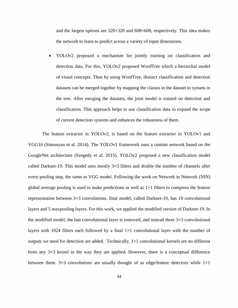
44
and the largest options are 320×320 and 608×608, respectively. This idea makes
the network to learn to predict across a variety of input dimensions.
YOLOv2 proposed a mechanism for jointly training on classification and
detection data. For this, YOLOv2 proposed WordTree which a hierarchal model
of visual concepts. Then by using WordTree, distinct classification and detection
datasets can be merged together by mapping the classes in the dataset to synsets in
the tree. After merging the datasets, the joint model is trained on detection and
classification. This approach helps to use classification data to expand the scope
of current detection systems and enhances the robustness of them.
The feature extractor in YOLOv2, is based on the feature extractor in YOLOv1 and
VGG16 (Simonyan et al. 2014). The YOLOv1 framework uses a custom network based on the
GoogleNet architecture (Szegedy et al. 2015). YOLOv2 proposed a new classification model
called Darknet-19. This model uses mostly 3×3 filters and double the number of channels after
every pooling step, the same as VGG model. Following the work on Network in Network (NIN)
global average pooling is used to make predictions as well as 1×1 filters to compress the feature
representation between 3×3 convolutions. final model, called Darknet-19, has 19 convolutional
layers and 5 maxpooling layers. For this work, we applied the modified version of Darknet-19. In
the modified model, the last convolutional layer is removed, and instead three 3×3 convolutional
layers with 1024 filters each followed by a final 1×1 convolutional layer with the number of
outputs we need for detection are added. Technically, 1×1 convolutional kernels are no different
from any 3×3 kernel in the way they are applied. However, there is a conceptual difference
between them. 3×3 convolutions are usually thought of as edge/feature detectors while 1×1

45
kernels can only combine activations of each feature vector. The interpretation of such an
operation is that it is simulating the effect of a fully connected layer, applied to each feature
vector. The number of output filters for our detection model is computed as follows:
We predict 5 boxes with 5 coordinates each and 1 class per box, so we have num of
boxes × (num of classes + coords) = 5 × (1 + 5) = 30 filters in last convolutional layer of the
network. We train the network for 960 epochs with a learning rate of 10-3. We use a weight
decay of 0.0005 and momentum of 0.9. Table 5.1 shows full description of the YOLOv2 model
applied for our work. Conv and Max terms represent Convolutional and maxpooling layers,
respectively. The Route layer is to bring finer grained features in from earlier in the network, and
the Reorg layer is to make these features match the feature map size at the later layer. The end
feature map is 13×13, the feature map from earlier is 26×26. The Reorg layer maps the 26×26
feature map onto a 13×13 feature map so that it can be concatenated with the feature maps at
13×13 resolution.
For this work, we inquired training YOLOv2 from scratch, and fine-tuning an existing
pre-trained YOLOv2 network, and then compared the results of both approach. For fine tuning
the pre-trained network, we applied the weights which were trained on ImageNet dataset, and the
number of epochs and other configuration parameters except learning rate remain the same as
training from scratch model. To fine tune the weights of pre-trained model, we choose learning
rate 10-4 because we except that the weights of the pre-trained network are relatively good and
we do not want to distort them too much and fast. To test YOLOV2 model, we use a Geforce
940MX GPU, and the test speed is an average of 6.06 frames per second for our test dataset.
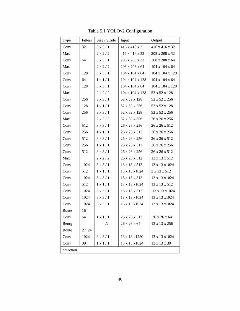
46
Table 5.1 YOLOv2 Configuration
Type Filters Size / Stride Input Output
Conv 32 3 x 3 / 1 416 x 416 x 3 416 x 416 x 32
Max 2 x 2 / 2 416 x 416 x 32 208 x 208 x 32
Conv 64 3 x 3 / 1 208 x 208 x 32 208 x 208 x 64
Max 2 x 2 / 2 208 x 208 x 64 104 x 104 x 64
Conv 128 3 x 3 / 1 104 x 104 x 64 104 x 104 x 128
Conv 64 1 x 1 / 1 104 x 104 x 128 104 x 104 x 64
Conv 128 3 x 3 / 1 104 x 104 x 64 104 x 104 x 128
Max 2 x 2 / 2 104 x 104 x 128 52 x 52 x 128
Conv 256 3 x 3 / 1 52 x 52 x 128 52 x 52 x 256
Conv 128 1 x 1 / 1 52 x 52 x 256 52 x 52 x 128
Conv 256 3 x 3 / 1 52 x 52 x 128 52 x 52 x 256
Max 2 x 2 / 2 52 x 52 x 256 26 x 26 x 256
Conv 512 3 x 3 / 1 26 x 26 x 256 26 x 26 x 512
Conv 256 1 x 1 / 1 26 x 26 x 512 26 x 26 x 256
Conv 512 3 x 3 / 1 26 x 26 x 256 26 x 26 x 512
Conv 256 1 x 1 / 1 26 x 26 x 512 26 x 26 x 256
Conv 512 3 x 3 / 1 26 x 26 x 256 26 x 26 x 512
Max 2 x 2 / 2 26 x 26 x 512 13 x 13 x 512
Conv 1024 3 x 3 / 1 13 x 13 x 512 13 x 13 x1024
Conv 512 1 x 1 / 1 13 x 13 x1024 3 x 13 x 512
Conv 1024 3 x 3 / 1 13 x 13 x 512 13 x 13 x1024
Conv 512 1 x 1 / 1 13 x 13 x1024 13 x 13 x 512
Conv 1024 3 x 3 / 1 13 x 13 x 512 13 x 13 x1024
Conv 1024 3 x 3 / 1 13 x 13 x1024 13 x 13 x1024
Conv 1024 3 x 3 / 1 13 x 13 x1024 13 x 13 x1024
Route 16
Conv 64 1 x 1 / 1 26 x 26 x 512 26 x 26 x 64
Reorg /2 26 x 26 x 64 13 x 13 x 256
Route 27 24
Conv 1024 3 x 3 / 1 13 x 13 x1280 13 x 13 x1024
Conv 30 1 x 1 / 1 13 x 13 x1024 13 x 13 x 30
detection

47
CHAPTER 6- CYCLIST TRACKING
Object visual tracking is the process of locating one or multiple identical objects in
continuous video frames or images sequences with temporal information. In automated video
analysis, detection of target objects, tracking them from frame to frame, and analysis of object
trajectories are important to recognize their behavior. So, visual tracking plays a crucial role in
various application such as (Yilmaz et al. 2006):
Motion-based object detection and recognition;
Automated video surveillance;
Gesture recognition or eye gaze tracking for human-computer interaction
application;
Automatic annotation and retrieval of the videos in multimedia databases;
Traffic monitoring to analysis safety measurements;
Medical image processing applications, such as labeling multiple cell in the
images;
Path planning and obstacle detection in vehicle automatic navigation.
Tracking methods should overcome some challenges such as:
Object’s scale variation
Object’s abrupt motion
Object’s shape variation due to in-plane and out of plane rotations

48
Information loss due to projection of 3D world on 2D video frames
Full and partial target occlusion
Scene illumination changes
Presence of noise and blur in video frames
To perform tracking in video sequences, an algorithm analyzes sequential video frames
and outputs the target movement between the frames. Many tracking algorithms have been
proposed based on available features such as motion and appearance. Since the convolutional
neural network features outperformed appearance based and motion based features, we use the
detection by YOLOv2 in the tracking phase.
In traffic monitoring, it is important to have a real-time tracker with the capability of
tracking multiple objects concurrently. The Kernelized Correlation Filter (KCF) is a robust and
real-time tracker introduced for single object tracking. We improved the capability of this tracker
using Bipartite Graph (BG) (Zhong et al. 2014) matching to perform multiple cyclist tracking.
So, the tracking system is a combination of the Kernelized Correlation Filter (KCF) and the BG
matching that solves the correspondence problem between multiple detections and multiple
tracks.
6.1. Kernelized Correlation Filter (KCF) Tracking
KCF is a Correlation Filter-based Tracker (CFT) which uses a discriminative classifier to
distinguish between the target object and its surrounding environment. CFTs have achieved
extremely compelling results in different competitions and benchmarks (Chen et al. 2015).

49
The general framework for all the existing CFTs is summarized in algorithm 6.1.
Algorithm 6.1: CFTs Tracking algorithm
In the first frame of the video data, correlation filter is trained with an image patch
cropped from a certain position of the target. If detection has been performed before
tracking, the image patch is the detected part of the target in a bounding box.
In subsequent frames, the patch at the previous predicted position is cropped for
detection
Various features can be extracted from the raw input and a cosine window is usually
applied for boundary effect smoothing
Efficient correlation operations are performed by element-wise multiplications using
Discrete Fourier Transform (DFT); the DFT of a vector is computed by the efficient
Fast Fourier Transform (FFT) algorithm
Following the correlation procedure, a spatial confidence map, or a response map, can
be obtained using inverse FFT.
The position with a maximum value in this map is then predicted as the new state of
the target
Appearance at the estimated position is extracted for training and updating the
correlation filter, and because only the DFT of the correlation filter is required for
detection, training and updating procedures are all performed in frequency domain
Compared to other CFTs, CSK and KCF take advantage of the kernel function, thus
correlation filters are supposed to be more powerful (Chen et al. 2015). Henriques et al. (2012)
proposed CSK method which uses kernel function. CSK method directly applies raw pixels as a
feature. When raw pixels are used for detection, various noises such as illumination changes and
motion blur limit the performance of the tracker. So, it is obvious that feature representing
method is an important factor of the performance of correlation based tracking methods.
Henriques et al. (2015) also proposed a method called KCF. In this method, the authors
improved the ability of a trained classifier by using multi-channel HOG as a feature instead of
raw pixel data. As it was mentioned, CFTs are tracking based on detection. For training the
detection model, positive samples are obtained based on the center of the target and negative
samples are extracted based on the surrounding areas of the target. Some of the CFTs use 1 to

50
label positive sample and 0 to label negative samples. But, KCF applies a weighted approach to
label the samples. In KCF, each sample gets a weighted label based on its distance from the
target. KCF method solves this sample training process as a ridge regression problem (Murphy
2012).
Formally, given training set (𝑥𝑖, 𝑦𝑖) for i=1,2, …, n, we want to create a regression model
that can predict label y for a new x. Therefore, for given training samples xi with regression
values (labels) yi, the training problem can be solved by minimizing a regularized cost function:
min𝑤∑ (𝑓(𝑥𝑖) − 𝑦𝑖)
2𝑖 + 𝜆‖𝑤‖2 Eq. 6.1
where 𝜆‖𝑤‖2 is regularization term and λ is a regularization parameter to avoid
overfitting, as in the Support Vector Machine. Here is the solution for Eq. 6.1 in complex fields:
𝑤 = (𝑋𝑇𝑋 + 𝜆𝐼)−1𝑋𝑇𝑦 Eq. 6.2
where X is a matrix whose rows are training samples, y is a vector of corresponding
regression values (labels), and I is identity matrix. If the computation is carried out in the
frequency domain, XT will be replaced by the Hermitian transpose of X in Eq. 6.2, which is XH =
(X∗) T.
As it was mentioned in (Henriques et al. 2015), using kernel function increases the
performance of the classifier. The input data 𝑥𝑖 can be mapped to a non-linear feature space with
𝜑(𝑥𝑖). w can be expressed as a linear combination of the inputs, and the variables under
optimization are thus α, instead of w:

51
𝑤 = ∑ 𝛼𝑖𝜑(𝑥𝑖)𝑖 Eq. 6.3
Then f(xi) can be written as:
𝑓(𝑥𝑖) = ∑ 𝛼𝑖𝑘(𝑥𝑖𝑛𝑗=1 , 𝑥𝑗) Eq. 6.4
where 𝑘(𝑥𝑖 , 𝑥𝑗) = ⟨𝜑(𝑥𝑖), 𝜑(𝑥𝑗)⟩ is the kernel function. The solution to the classical
kernelized ridge regression can be given by:
𝛼 = (𝐾 + 𝜆𝐼)−1𝑦 Eq. 6.5
Where 𝜆 is regularization parameter, I is identity matrix, and K is the kernel matrix with
dot-product in Hilbert space as its elements 𝑘(𝑥𝑖, 𝑥𝑗).
Some methods generate more templates by random sampling patches around the first
patch to collect more training data. On the other hand, KCF applies a circulant matrix to collect
all the translated samples around the object at a lower time.
Suppose we have a vector X= [x1 x2 … xn]. By circular shift, we could get the vector [xn x2
… xn-1]. We can obtain these vectors which can constitute a circular matrix by shifting operation,
as shown below:
𝑋 = 𝐶(𝑥) = [
𝑥1𝑥𝑛
𝑥2𝑥1
⋯⋯
𝑥𝑛𝑥𝑛−1
⋮ ⋮ ⋱ ⋮𝑥2 𝑥3 ⋯ 𝑥1
] Eq. 6.6
Henriques et al. (2015) proved that most of the kernel function matrices are cyclic
matrices. Therefore, Eq. 6.5 can be converted to the frequency domain by using the properties of
the circular matrix, as shown below:

52
�̂� =�̂�
�̂�𝑥𝑥+𝜆 Eq. 6.7
Here 𝐾𝑥𝑥 is the first row vector of the cyclic matrix K. The hat symbol ˆ represents the
Fourier transformation of a vector. For convenience, they also give three most typical kernel
functions qualified for the theory, namely, Polynomial kernel, Gaussian kernel and Linear kernel.
When selecting a linear kernel, the problem is reduced to the original regression problem. Once
securing or initializing the target patch 𝑥′, the kernel matrix in the frequency domain is
calculated:
𝐾𝑥𝑥′= (𝐹−1(�̂� ⊙ �̂�′∗) + 𝑎)𝑏 Eq. 6.8
𝐾𝑥𝑥′= (−
1
𝛿2exp ((‖𝑥‖2‖𝑥′‖2 − 2𝐹−1(�̂�⨀�̂�′∗))) Eq. 6.9
Here Eq. 6.8 is for Polynomial kernel and Eq. 6.9 is for Gaussian kernel. ⊙ denotes
element-wise multiplication and * means the complex conjugate of a vector. The vector x
represents the appearance model and in the first coming frame, x is initialized to 𝑥′. In this work,
the Gaussian kernel is used.
In a new frame, the target can be detected by the trained parameter α and a maintained
base sample x. If the new sample is z, a confidence map y can be obtained by:
𝑦 = 𝐶(𝐾𝑥𝑧)𝛼 = 𝐹−1(�̂�𝑥𝑧⨀�̂�) Eq. 6.10
The position with a maximum value in y can be predicted as new position of the target.
As it is demonstrated in Figure 6.1, the tracker handles short-term partial occlusion
(Figure 6.1 (1)) but it cannot overcome full occlusions (Figure 6.1 (2)).

53
Figure 6.1 Tracking in cases with occlusions - (1) partial occlusion, (2) full occlusion
6.2. Multiple Object Tracking
Multiple object tracking (MOT) is partitioned to locating multiple objects, maintaining
their identities and yielding their individual trajectories given an input video. Multiple object
tracking is a challenging task because of the variable number of target objects and the interaction
between them in complex dynamic environments. For multiple object tracking after finding
object location in the next frame, the locations are compared to all positions of the detected
object. This comparison is done by data association. The technique of data association figures out
inter-frame correspondences between detection hypothesis and existing tracks.
In our tracking method, data association was solved by bipartite graph matching
algorithm (Zhong et al. 2014): the nodes of the bipartite graph correspond to the detected cyclists
and existing tracks, and the weighted edges of the bipartite graph are marked by the cost of
detection-track matching. The correspondence between detected cyclists and existing tracks is
solved by the dynamic Hungarian matching algorithm to determine the maximum matching
results.

54
In the bipartite graph, each node is denoted by 𝐷𝑖 = {𝑃𝑖} which is the centroid position.
The cost function for data association is computed by:
𝑆(𝐷𝑖 , 𝐷𝑗) = √(𝑥1 − 𝑥2)2 + (𝑦1 − 𝑦2)2 Eq. 6.12
Where Di and Dj represent centroid position of detection nodes and centroid position of
tracking node, respectively, and S is Euclidian distance between two nodes. If the cost function S
is small, the two nodes are more likely to have correspondence. The threshold value for cost
function S is 35. It means that if 𝑆(𝐷𝑖 , 𝐷𝑗) is lesser than 35, there will be a match.
MOT can handle miss detections and false detections. Every detected cyclist is passed to
the tracking system, and a new KCF track is initialed for it. Then, every new track is updated by
the KCF in the subsequent frames and the information of each track is saved in a tracking table
until it is deleted from the list of lost tracks.
The tracking table is a data structure which keeps the record of tracking parameters.
These parameters are:
Track Identifier (ID): ID parameter identifies each track and is used for track
association
Bounding Box: bounding box coordinates of the track at each frame
Centroid: centroid stores the center points of the bounding box of the track in each
frame
Tracking Age: tracking age shows the number of frames since the track was
initialized

55
Visible Length: it is the number of frames in which track was detected
Invisible Length: it is the number of consecutive frames in which track was not
detected
Visibility Ratio: visible length/ tracking age
KCF parameters: stores KCF tracker parameters
The tracking age, visible length, invisible length and visibility ratio (visible length/
tracking age) are used to handle miss detections and false detections. To prevent short tracks
caused by false detections, the visible length will be compared to a threshold (here, 10 frames). If
the invisible length is less than that threshold, its track will not be stored or displayed. A track
will be deleted if its visible length exceeds a threshold (here, 5 frames) or it is a young track
(tracking age <7) whose invisibility ratio is lesser than a threshold (here, 0.5). This is helpful to
stop tracking non-targets or targets who left the view, and continue tracking targets even they
have some miss detections. The parameters are set experimentally. Figure 6.2. describes the
flowchart of procedures of the cyclist tracking system.

56
Figure 6.2 Cyclist tracking system flowchart

57
CHAPTER 7- CYCLIST COUNTING
Cyclists use both intersection and road, and their movements follow various patterns,
including the road crossings at any location and angles. Compared to pedestrians whose
movement across the road is predetermined, cyclists are not necessarily restricted and can cross
intersections diagonally and can appear beyond or in front of pedestrians from the camera view
point. Their turning angles change more frequently compared to that of cars or pedestrians, due
to the higher mobility. So, the counting method which is used for cyclist should be able to collect
not only the crossing counts but also the turning movement counts of cyclists. In contrast to LOI-
based and ROI-based counting methods, the trajectory based approach promises robust
identifications of various movement directions.
For the safety analysis, it is imperative to obtain fine statistics about not only cyclists at
the intersection as whole, but counts in specific locations. It is important to identify possible
conflicts that can be derived from the analyses of virtual crossings of car and bicycle paths. For
that, the system is to be able identify the cyclists on a specific path. The consideration of
reconstructed trajectories is expected to lead to more accurate counts as it is able to eliminate
false detections and short motion segments. All possible paths of cyclist on the intersection
(likewise on the street) are defined as POI (Path of Interest). The counting method that we have
developed is based on establishing the similarity of cyclist trajectories and POIs and for that the
choice of the similarity metric is essential. One can choose either geographic similarity or
semantic similarity. Geographic similarity captures spatial adjacency of the trajectories, whereas
semantic similarity captures shape difference of trajectories (Ra et al. 2015). For the real scenes,
due to various shapes of trajectories, semantic methods have a better discriminative power over

58
geographic metric (Liu et al. 2012). For that reason, we use semantic similarity, specifically, the
Longest Common Subsequence (LCSS). For evaluating similarity, we must obtain trajectories of
a sufficient length, and for that a trajectory rebuilding method is used (Idrissov et al. 2012).
7.1. Trajectory Rebuilding
Trajectories can be reconstructed from segments if some parts are missing. These missing
parts of a trajectory are those which were not recorded due to the loss of track. The idea of
trajectory rebuilding helps connecting trajectory segments made by a single cyclist. Trajectory
rebuilding tries to find matches based on spatiotemporal proximity. Spatiotemporal proximity
method inquires the Euclidian distance and the frame interval of the missing segment endpoints.
Spatial and temporal thresholds, here, α and β are to be set.
After finding corresponding parts of the trajectory, a missing segment interpolation
method (Idrissov et al. 2012) is used to connect them and complete the trajectory. The
motivation behind this is that for the POI comparison we need trajectories of a certain length that
would consider only cyclist’s movement and neglect false trajectories. A sufficient length
trajectory is one which is of a length sufficient to recognize forward direction and turns. If
sufficient length threshold is set to a high value, it would eliminate false counting caused by false
detections and multiple counting caused by broken segments of a single cyclist trajectory. But, if
we have a high value of the threshold for the sufficient length, reliable short broken trajectories
caused by miss detections, occlusions, and tracking flaw will be ignored for counting purpose.
Thus, a high value of the threshold along with a robust trajectory rebuilding make a robust
counting method which reduce multiple counting of a single object, false counting due to false
detections, and loss of counting because of miss detections, occlusion, and the tracker flaws. In

59
this work, the sufficient length has been defined as at least 30 consecutive frames. If the length
of rebuilt trajectories is lesser than the sufficient length, it will not be used towards counting.
Figure 7.1 shows two trajectories of cyclists that can be considered of a sufficient length.
Figure 7.1 Cyclist’s trajectories of “sufficient” lengths
Let Ps and Pend be the ending location of trajectory 1 and the starting location of
trajectory 2 to be matched. Timestamps of these two points are Ts and Tend, respectively. If the
difference between Ts and Tend is lesser than β, which is 10 frames, and the difference between Ps
and Pend is lesser than α, which is 110, we use interpolation to connect trajectory 1 to trajectory 2.
If these differences exceed either or both thresholds, we count them as two separate trajectories.
For interpolation, we first estimate the number of sub-segments Ns that is necessary
for uniform distribution of points across the whole missing segment (Idrissov et al. 2012).

60
𝑁𝑠 = [2×𝑛×𝐷(𝑃𝑠 , 𝑃𝑒𝑛𝑑)
∑ 𝐷(𝑃𝑎 ,𝑃𝑎+1)𝑠−1𝑎=𝑠−𝑛 + ∑ 𝐷(𝑃𝑎 ,𝑃𝑎+1)
𝑒𝑛𝑑+𝑛−1𝑎=𝑒𝑛𝑑
] Eq. 7.1
where, D is Euclidian distance between two endpoints, Ps and Pend of missing segment,
and n is the number of previous points and next points of both sides of missing segments that are
used for interpolation. We choose n = 5 for the algorithm implementation.
The distance between two consecutive points is defined as follows:
𝐼𝑛𝑡𝑒𝑟𝑣𝑎𝑙 =𝐷(𝑃𝑠 , 𝑃𝑒𝑛𝑑)
𝑁𝑠 Eq. 7.2
At the end, we create Ns−1 points between Ps and Pend according to the calculated
interval distance.
7.2. POI model
In the POI comparison model, we have applied LCSS algorithm. Compared to other
semantic similarity measurement methods, LCSS performs better for unequal length trajectories,
outliers, different sampling rates of the camera and different object velocities (Buzan et al.
2004). In this model, each cyclist trajectory is compared to all POIs which are detected in the
scene. A POI with a highest similarity and a lowest distance is chosen as a best matching path,
and the counter for the cyclist is incremented for the selected POI.
We employ the 2D LCSS algorithm (Buzan et al. 2004). Let F and G be two 2D
trajectories of lengths m and n, respectively.

61
𝐹 = ((𝑓𝑥,1 , 𝑓𝑦,1), … , (𝑓𝑥,𝑛 , 𝑓𝑦,𝑛) ) Eq. 7.3
𝐺 = ((𝑔𝑥,1 , 𝑔𝑦,1), … , (𝑔𝑥,𝑚 , 𝑔𝑦,𝑚) ) Eq. 7.4
Head(G) and Head(F) are defined as follows.
𝐻𝑒𝑎𝑑(𝐺) = ((𝑔𝑥,1 , 𝑔𝑦,1),… , (𝑔𝑥,𝑚−1 , 𝑔𝑦,𝑚−1) ) Eq. 7.5
𝐻𝑒𝑎𝑑(𝐹) = ((𝑓𝑥,1 , 𝑓𝑦,1), … , (𝑓𝑥,𝑛−1 , 𝑓𝑦,𝑛−1) ) Eq. 7.6
Then, the 𝐿𝐶𝑆𝑆𝛿, (𝐹𝑥, 𝐺𝑥) and 𝐿𝐶𝑆𝑆2𝐷(𝛿, 휀, 𝜌, 𝐹, 𝐺) are defined as follows.
𝐿𝐶𝑆𝑆𝛿, (𝐹𝑥, 𝐺𝑥) =
{
0 𝑖𝑓 𝐹 𝑜𝑟 𝐺 𝑖𝑠 𝑒𝑚𝑝𝑡𝑦
1 + 𝐿𝐶𝑆𝑆𝛿, (𝐻𝑒𝑎𝑑(𝐹𝑥), 𝐻𝑒𝑎𝑑(𝐺𝑥))
𝑖𝑓 |𝑓𝑥,𝑛 , 𝑔𝑥,𝑚| < 휀 a𝑛𝑑 |𝑛 − 𝑚| < 𝛿
max (𝐿𝐶𝑆𝑆𝛿, (𝐻𝑒𝑎𝑑(𝐹𝑥), 𝐺𝑥), 𝐿𝐶𝑆𝑆𝛿, (𝐹𝑥, 𝐻𝑒𝑎𝑑(𝐺𝑥)))
𝑜𝑡ℎ𝑒𝑟𝑤𝑖𝑠𝑒
Eq. 7.7
𝐿𝐶𝑆𝑆2𝐷(𝛿, 휀, 𝜌, 𝐹, 𝐺) =
{
(0,0) 𝑖𝑓 min{m, n} < 𝜌.max {𝑚, 𝑛}
(𝐿𝐶𝑆𝑆𝛿, (𝐹𝑥 , 𝐺𝑥) , 𝐿𝐶𝑆𝑆𝛿, (𝐹𝑦, 𝐺𝑦))
𝑜𝑡ℎ𝑒𝑟𝑤𝑖𝑠𝑒
Eq. 7.8
Here, ρ is the aspect ratio which controls the differences in the size of two trajectories.
And, the parameter δ controls how far in time we can go to the past to match a given point from
one of trajectory to a point in another trajectory. And ε is a matching threshold.
The similarity function 𝑆2𝐷(𝛿, 휀, 𝐹, 𝐺) between two trajectories F and G is defined as
follows:

62
𝑆2𝐷(𝛿, 휀, 𝐹, 𝐺) = (𝐿𝐶𝑆𝑆𝛿, (𝐹𝑥,𝐺𝑥)
min (𝑚,𝑛),𝐿𝐶𝑆𝑆𝛿, (𝐹𝑦,𝐺𝑦)
min (𝑚,𝑛)) Eq. 7.9
We define the distance function which is used for comparing POIs and cyclist
trajectories, with the given δ and ε:
𝐷2𝐷(𝛿, 휀, 𝐹, 𝐺) =(1−
𝐿𝐶𝑆𝑆𝛿, (𝐹𝑥,𝐺𝑥)
min(𝑚,𝑛))+(1−
𝐿𝐶𝑆𝑆𝛿, (𝐹𝑦,𝐺𝑦)
min(𝑚,𝑛))
2 Eq. 7.10
D is a symmetric function because 𝑆2𝐷(𝛿, 휀, 𝐹, 𝐺) is equal to 𝑆2𝐷(𝛿, 휀, 𝐺, 𝐹). Each
reconstructed trajectory is compared to all POIs, and the POI with a smallest D2D value is chosen
as a best match.
The POIs shown in Figure 7.2 are constructed based on the first complete or rebuilt
trajectory for each direction. Distance between points in one POI is based on the distance of that
POI to the camera. For example, the connected points in INT are closer to each other than those
in WE, and this is due to projection of 3D world on 2D video frames. POIs with specific
location/direction are marked with different colors. There are Intersection (INT), and directions
in the road segments: East-West (EW), West-East (WE), North-East (NE), North-West (NW),
and West-North(WN). Note that in EW and WE directions in contrast to other directions, cyclists
are free to move within a large road segment. Therefore, we define more than one POI for EW
and WE directions. The POIs are used for LCSS trajectory comparison.

63
Figure 7.2 Paths of Interest (POIs)

64
CHAPTER 8- EXPERIMENTS AND RESULTS
To evaluate the performance of the detection, tracking, and counting systems, 8300
frames from Nevada datasets which contain the most number of cyclists were manually
annotated. The measurements which are used to evaluate the performance of detection systems
are true positive detection (TP), false positive detection (FP) or false alarm, false negative
detection (FN) or miss detection, true positive rate (TPR) or recall, precision, false positive per
frame (FPPF), and false negative per frame (FNPF). All the parameters are calculated as follow:
𝑇𝑃𝑅 (𝑟𝑒𝑐𝑎𝑙𝑙) =𝑇𝑃
𝑇𝑃+𝐹𝑁 Eq. 8.1
𝑝𝑟𝑒𝑐𝑖𝑠𝑖𝑜𝑛 = 𝑇𝑃
𝑇𝑃+𝐹𝑃 Eq. 8.2
𝐹𝑃𝑃𝐹 =𝐹𝑃
𝑁𝑓𝑟𝑎𝑚𝑒𝑠 Eq. 13
𝐹𝑁𝑃𝐹 =𝐹𝑁
𝑁𝑓𝑟𝑎𝑚𝑒𝑠 Eq. 8.4
where TP is the number of cyclists correctly predicted to be cyclists; FP is the number of
non-cyclists incorrectly predicted to be cyclists; FN is the number of cyclists incorrectly
predicted to be non-cyclists; 𝑁𝑓𝑟𝑎𝑚𝑒𝑠 is the total number of frames in the corresponding test
video. The precision is the fraction of positive detections that is an actual positive hit
(ground truth). The TPR or recall is the probability that a ground truth object is recognized by the
detector. In a detection system, TPR and precision close to 1 and lower FPPF and FNPF are
indicators of better detection accuracy.

65
8.1. Performance of Classification
To demonstrate how the performance of the trained model is improved if the SVM is fed
by the combined feature vector, 20% of vertical and horizontal views of type A and type B
datasets were used to test each trained model. To evaluate the classification performance, the
area under the ROC curve (AUC) per feature is computed. AUC is used in classification analysis
to determine which of the models predicts the classes best. In ROC curve, the true positive rates
are plotted against false positive rates. Table 8.1 shows the area under the ROC curve for each
model. It can be observed that classification results most of the time are improved for the
combined features. Because HOG-MLBP feature for horizontal view of dataset type B showed a
better result compared to other features and dataset types, we use this model for testing. Finally,
the detection result of this model is compared to that obtained by YOLOv2 model.
Table 8.1 Area Under ROC Curve (AUC) for each feature
Dataset View HOG MLBP HSC HOG-MLBP HOG-HSC
Type A
Horizontal 0.9815 0.9890 0.9865 0.9903 0.9875
Vertical 0.8286 0.9099 0.8788 0.9083 0.8609
Type B
Horizontal 0.9961 0.9972 0.9891 0.9989 0.9900
Vertical 0.9657 0.9918 0.9809 0.9831 0.9710
8.2. Performance of Detection
The detection and tracking performance is evaluated on the annotated test frames from
the Nevada dataset. To fine tune pre-trained YOLOv2 and train YOLOv2 from the scratch, we

66
used the horizontal view of dataset type B. The detection performance results are demonstrated
in Table 8.2. One can see that the pre-trained YOLOv2 model yields a better detection
performance. The precision values of the both pre-trained YOLOv2 and YOLOv2 trained with
random initialization are identical. But the recall value in the pre-trained model has been
improved significantly. The precision value for the combined feature which is fed into SVM
classifier is inferior to two other methods, and its recall value is not significantly different from
one by the trained YOLO model.
Table 8.2 Detection result
Method of detection TPR(recall) precision FPPF FNPF
Yolov2 (fine tuning) 0.83 0.99 0.005 0.14
Yolov2 (trained from scratch) 0.59 0.99 0.005 0.33
GMM +MLBP-HOG + SVM 0.56 0.4 0.67 0.35
The detection errors are tried to be handled in further steps and do not affect the overall
performance of the counting method. It is obvious that fine tuning the pre-trained network works
better than the training the network from scratch. Detection examples of all three methods are
shown in Figures 8.1 and 8.2.

67
Figure 8.1 Detection examples by (1) pre-trained YOLOv2, (2) YOLOv2 trained from scratch,
(3) Combined GMM-HOG-MLBP

68
Figure 8.2 Detection examples by (1) pre-trained YOLOv2, (2) YOLOv2 trained from scratch,
(3) Combined GMM-HOG-MLBP
8.3. Performance of Tracking
To evaluate the performance of tracking, we use the criteria defined by Wu et. al (2007).
MT: number of "mostly tracked" trajectories (more than 80 % of cyclist trajectory is
tracked),
ML: number of "mostly lost" trajectories (more than 80 % of cyclist trajectory is lost),

69
FRG: number of "fragments" of trajectories (a result trajectory which between 40 % and
80% of the ground truth trajectory),
FT: number of "false trajectories" (a result trajectory corresponding to non-target object).
GT: number of "ground truth" trajectories.
The employed tracking system performs well by all criteria. It displays high MT value
and low ML, FG, and FT values. Table 8.3 shows the results by the proposed tracker. The
tracking result represents a good performance of the tracker. We also provide the number of
segments for each of existing paths to substantiate the need in trajectory rebuilding. Table 8.4
shows the number of broken segments per path direction. As the number of broken segments is
lower, there is a lesser need in trajectory rebuilding. Some examples of tracking are shown in
Figure 8.3.
Table 8.3 The tracking result
Tracking method GT MT ML FT FRG
YOLO+ KCF MOT 39 32 1 1 6
Table 8.4 Number of broken segments for each path direction
Paths Ground truth
Number of broken segments
YOLO+KCF MOT
0 1 2 3 4
EW 6 1 4 1 0 0
WE 5 3 2 0 0 0
WN 4 4 0 0 0 0

70
NW 7 2 4 0 0 0
NE 1 0 1 0 0 0
INT 16 1 8 5 0 2
Figure 8.3 Tracking examples, the distance between centroids is based on the cyclist’s velocity
and the distance between cyclist and the camera.

71
8.4. Performance of Counting
The measurements used to evaluate the performance of counting method are True
Positive Counting (TPC) and False Positive Counting (FPC). TPC is the number of cyclists’
trajectories assigned to a correct POI. FPC is the number of trajectories assigned to a wrong POI
or assigned to a correct POI more than one time for previously estimated trajectories. FPC is
used to show not only incorrect counting but also multiple counting for a single cyclist produced
mostly due to broken trajectories.
As it is shown in Table 8.4, most of the trajectories have at least one broken segment. If
these broken segments are not reconstructed by trajectory rebuilding method, with a small
threshold of the sufficient length parameter, there will be a high number of FPCs.
We compare the accuracy of counting method before and after the trajectory rebuilding.
The system is robust if TPC is closer to the ground truth of counting and FPC is close to 0. As it
shown in Table 8.5, the accuracy of the counting system has been improved by trajectory
rebuilding methodology. Figure 8.4 displays examples of trajectory rebuilding. The red dots
show the incomplete trajectory, and green dots display interpolated points which fill out the
gaps; the blue lines show complete trajectories after interpolation.
Table 8.5 Counting result (before/after) trajectory rebuilding
Path of Interest EW WE WN NW NE INT
Ground Truth 6 5 4 7 1 16
TPC 6/6 3/4 3/3 4/5 1/1 11/15
FPC 3/0 2/1 6/2 4/0 1/1 8/2

72
Figure 8.4 Examples of trajectory rebuilding (to be viewed in color)

73
CHAPTER 9- CONCLUSION AND FUTURE WORK
9.1. Summary of work
In this work, we presented a novel system that performs cyclist detection, tracking,
trajectory reconstruction and counting at road segments and intersections. The detection system
employed a multi-feature classifier for vertically and horizontally oriented cyclists. A CNN
based detection method called YOLO was also implemented to enhance the accuracy of cyclist
detection. Compared to HOG-MLBP fed into SVM, YOLO showed a better performance in
cyclist detection. Therefore, its detection output, i.e., bounding boxes were used for the tracking
task. The multi-object tracker implemented using KCF and the bipartite graph matching methods
has been robust in the presence of short-term partial occlusions and cyclist’s abrupt moves. The
trajectory constructed from centroids of tracking bounding boxes was used for counting task. For
counting, a trajectory rebuilding methodology was applied to modify the resultant trajectories
from the tracking step. Then, the counting model evaluated the similarity between rebuilt
trajectories and certain paths of interests. The rebuilding trajectory method was incorporated into
the system to improve the counting accuracy. The counting method showed a high performance
in counting the number in crossings and the number in turning movements. The trajectory data
collected through this experiment can be used for road safety studies.
9.2. Future work
Vision based data collection, analyses and road monitoring is a topic of a growing interest in
Intelligent Transportation Systems (ITS). The collected data and the designed methodology can
be used for future needs.

74
In the safety analyses, road user trajectories are used to compute measures such as Time
To Collision (TTC), Post Encroachment Time (PET), and Gap time. Therefore, the trajectories
found by the system designed in this work can be used for deriving safety measures for cyclists.
For improving the performance of YOLO detector, the detector should be trained with a
larger dataset. Therefore, it is better to collect more cyclist data for future training.
One of the challenging problem researchers have been facing in object tracking is the
problem of partial and full occlusions. The developed multi object tracking (MOT) KCF has
ability to handle sort-term partial occlusions. The future methods will include those which can
handle a larger degree of occlusion.
Monitoring systems presented in the literature are designed to work under the day light
conditions. Enhancing the ability of the system to detect and track cyclists at night by analyzing
thermal images.
Several CNN-based classification and detection methods have been developed recently.
Their performance for the cyclist detection in traffic video data is to be evaluated based on
accuracy and speed metrics.
75
REFERENCES
TRAFFIC SAFETY FACTS 2014, National Highway Traffic Safety Administration
(NHTSA).
Zangenehpour, S., Romancyshyn, T., Miranda-Moreno, L. F., & Saunier, N. (2015). Video-
based automatic counting for short-term bicycle data collection in a variety of environments.
In Transportation Research Board 94th Annual Meeting (No. 15-4888).
Ryan, S., & Lindsey, G. (2013). Counting bicyclists and pedestrians to inform transportation
planning. Princeton, NJ: Robert Wood Johnson Foundation.
Chan, Y. T., Hu, A. G. C., & Plant, J. B. (1979). A Kalman filter based tracking scheme with
input estimation. IEEE transactions on Aerospace and Electronic Systems, (2), 237-244.
Robert, K. (2009, September). Night-time traffic surveillance: A robust framework for multi-
vehicle detection, classification and tracking. In Advanced Video and Signal Based
Surveillance, 2009. AVSS'09. Sixth IEEE International Conference on (pp. 1-6). IEEE.
Shahraki, F. F., Yazdanpanah, A. P., Regentova, E. E., & Muthukumar, V. (2015,
December). Bicycle Detection Using HOG, HSC and MLBP. In International Symposium on
Visual Computing (pp. 554-562). Springer International Publishing.
Pucher, J., Buehler, R., & Seinen, M. (2011). Bicycling renaissance in North America? An
update and re-appraisal of cycling trends and policies. Transportation research part A: policy
and practice, 45(6), 451-475.
Strauss, J., Miranda-Moreno, L. F., & Morency, P. (2014). Multimodal injury risk analysis of
road users at signalized and non-signalized intersections. Accident Analysis &
Prevention, 71, 201-209.
Sivaraman, S., & Trivedi, M. M. (2013). Looking at vehicles on the road: A survey of
vision-based vehicle detection, tracking, and behavior analysis. IEEE Transactions on
Intelligent Transportation Systems, 14(4), 1773-1795.
Gandhi, T., & Trivedi, M. M. (2007). Pedestrian protection systems: Issues, survey, and
challenges. IEEE Transactions on intelligent Transportation systems, 8(3), 413-430.
Dharmaraju, R., Noyce, D. A., & Lehman, J. D. (2001, August). An evaluation of
technologies for automated detection and classification of pedestrians and bicycles. In The
71st ITE Annual Meeting.
Geronimo, D., Lopez, A. M., Sappa, A. D., & Graf, T. (2010). Survey of pedestrian detection
for advanced driver assistance systems. IEEE transactions on pattern analysis and machine
intelligence, 32(7), 1239-1258.

76
Viola, P., & Jones, M. (2001). Rapid object detection using a boosted cascade of simple
features. In Computer Vision and Pattern Recognition, 2001. CVPR 2001. Proceedings of the
2001 IEEE Computer Society Conference on (Vol. 1, pp. I-I). IEEE.
Dalal, N., & Triggs, B. (2005, June). Histograms of oriented gradients for human detection.
In Computer Vision and Pattern Recognition, 2005. CVPR 2005. IEEE Computer Society
Conference on (Vol. 1, pp. 886-893). IEEE.
Wang, L., & He, D. C. (1990). Texture classification using texture spectrum. Pattern
Recognition, 23(8), 905-910.
Lowe, D. G. (2004). Distinctive image features from scale-invariant keypoints. International
journal of computer vision, 60(2), 91-110.
Felzenszwalb, P. F., Girshick, R. B., McAllester, D., & Ramanan, D. (2010). Object
detection with discriminatively trained part-based models. IEEE transactions on pattern
analysis and machine intelligence, 32(9), 1627-1645.
Cho, H., Rybski, P. E., & Zhang, W. (2010, September). Vision-based bicycle detection and
tracking using a deformable part model and an EKF algorithm. In Intelligent Transportation
Systems (ITSC), 2010 13th International IEEE Conference on (pp. 1875-1880). IEEE.
Jung, H., Ehara, Y., Tan, J. K., Kim, H., & Ishikawa, S. (2012, October). Applying MSC-
HOG Feature to the Detection of a Human on a Bicycle. In Control, Automation and Systems
(ICCAS), 2012 12th International Conference on (pp. 514-517). IEEE.
Schapire, R. E., & Singer, Y. (1999). Improved boosting algorithms using confidence-rated
predictions. Machine learning, 37(3), 297-336.
Dahiya, K., Singh, D., & Mohan, C. K. (2016, July). Automatic detection of bike-riders
without helmet using surveillance videos in real-time. In Neural Networks (IJCNN), 2016
International Joint Conference on (pp. 3046-3051). IEEE.
Zivkovic, Z. (2004, August). Improved adaptive Gaussian mixture model for background
subtraction. In Pattern Recognition, 2004. ICPR 2004. Proceedings of the 17th International
Conference on (Vol. 2, pp. 28-31). IEEE.
Lin, Y. B., & Young, C. P. (2017). High-precision bicycle detection on single side-view
image based on the geometric relationship. Pattern Recognition, 63, 334-354.
Fujimoto, Y., & Hayashi, J. I. (2013, January). A method for bicycle detection using ellipse
approximation. In Frontiers of Computer Vision, (FCV), 2013 19th Korea-Japan Joint
Workshop on (pp. 254-257). IEEE.
Hu, W., Tan, T., Wang, L., & Maybank, S. (2004). A survey on visual surveillance of object
motion and behaviors. IEEE Transactions on Systems, Man, and Cybernetics, Part C
(Applications and Reviews), 34(3), 334-352.

77
Sugandi, B., Kim, H., Tan, J. K., & Ishikawa, S. (2007, September). Tracking of moving
objects by using a low-resolution image. In Innovative Computing, Information and Control,
2007. ICICIC'07. Second International Conference on (pp. 408-408). IEEE.
Li, J., Shao, C., Xu, W., & Dong, C. (2009, April). Real-time pedestrian detection based on
improved gaussian mixture model. In Measuring Technology and Mechatronics Automation,
2009. ICMTMA'09. International Conference on (Vol. 3, pp. 269-272). IEEE.
Girshick, R., Donahue, J., Darrell, T., & Malik, J. (2014). Rich feature hierarchies for
accurate object detection and semantic segmentation. In Proceedings of the IEEE conference
on computer vision and pattern recognition (pp. 580-587).
Girshick, R. (2015). Fast r-cnn. In Proceedings of the IEEE International Conference on
Computer Vision (pp. 1440-1448).
Ren, S., He, K., Girshick, R., & Sun, J. (2015). Faster r-cnn: Towards real-time object
detection with region proposal networks. In Advances in neural information processing
systems (pp. 91-99).
Redmon, J., Divvala, S., Girshick, R., & Farhadi, A. (2016). You only look once: Unified,
real-time object detection. In Proceedings of the IEEE Conference on Computer Vision and
Pattern Recognition (pp. 779-788).
Li, X., Flohr, F., Yang, Y., Xiong, H., Braun, M., Pan, S., & Gavrila, D. M. (2016, June). A
new benchmark for vision-based cyclist detection. In Intelligent Vehicles Symposium (IV),
2016 IEEE (pp. 1028-1033). IEEE.
Li, X., Li, L., Flohr, F., Wang, J., Xiong, H., Bernhard, M., & Li, K. (2017). A Unified
Framework for Concurrent Pedestrian and Cyclist Detection. IEEE Transactions on
Intelligent Transportation Systems, 18(2), 269-281.
Yilmaz, A., Javed, O., & Shah, M. (2006). Object tracking: A survey. Acm computing
surveys (CSUR), 38(4), 13.
Banerjee, S. P., & Pallipuram, K. (2008). Multi-person Tracking Using Kalman Filter.
Cho, H., Rybski, P. E., & Zhang, W. (2010, September). Vision-based bicycle detection and
tracking using a deformable part model and an EKF algorithm. In Intelligent Transportation
Systems (ITSC), 2010 13th International IEEE Conference on (pp. 1875-1880). IEEE.
Cho, H., Rybski, P. E., & Zhang, W. (2010, June). Vision-based bicyclist detection and
tracking for intelligent vehicles. In Intelligent Vehicles Symposium (IV), 2010 IEEE (pp.
454-461). IEEE.
J Shi, J. (1994, June). Good features to track. In Computer Vision and Pattern Recognition,
1994. Proceedings CVPR'94., 1994 IEEE Computer Society Conference on (pp. 593-600).
IEEE.

78
Sato, K., & Aggarwal, J. K. (2004). Temporal spatio-velocity transform and its application to
tracking and interaction. Computer Vision and Image Understanding, 96(2), 100-128.
Chen, Z., Hong, Z., & Tao, D. (2015). An experimental survey on correlation filter-based
tracking. arXiv preprint arXiv:1509.05520.
Henriques, J. F., Caseiro, R., Martins, P., & Batista, J. (2015). High-speed tracking with
kernelized correlation filters. IEEE Transactions on Pattern Analysis and Machine
Intelligence, 37(3), 583-596.
Chan, A. B., & Vasconcelos, N. (2012). Counting people with low-level features and
Bayesian regression. IEEE Transactions on Image Processing, 21(4), 2160-2177.
Li, J., Huang, L., & Liu, C. (2011, August). Robust people counting in video surveillance:
Dataset and system. In Advanced Video and Signal-Based Surveillance (AVSS), 2011 8th
IEEE International Conference on (pp. 54-59). IEEE.
Ryan, D., Denman, S., Fookes, C., & Sridharan, S. (2009, December). Crowd counting using
multiple local features. In Digital Image Computing: Techniques and Applications, 2009.
DICTA'09. (pp. 81-88). IEEE.
Zhang, Z., Liu, K., Gao, F., Li, X., & Wang, G. (2016, July). Vision-based vehicle detecting
and counting for traffic flow analysis. In Neural Networks (IJCNN), 2016 International Joint
Conference on (pp. 2267-2273). IEEE.
Zhou, B., Lu, M., & Wang, Y. (2016, May). Counting people using gradient boosted trees.
In Information Technology, Networking, Electronic and Automation Control Conference,
IEEE (pp. 391-395). IEEE.
Cao, J., Sun, L., Odoom, M. G., Luan, F., & Song, X. (2016, May). Counting people by using
a single camera without calibration. In Control and Decision Conference (CCDC), 2016
Chinese (pp. 2048-2051). IEEE.
Cong, Y., Gong, H., Zhu, S. C., & Tang, Y. (2009, June). Flow mosaicking: Real-time
pedestrian counting without scene-specific learning. In Computer Vision and Pattern
Recognition, 2009. CVPR 2009. IEEE Conference on (pp. 1093-1100). IEEE.
Yam, K. Y., Siu, W. C., Law, N. F., & Chan, C. K. (2011, January). Effective bi-directional
people flow counting for real time surveillance system. In Consumer Electronics (ICCE),
2011 IEEE International Conference on (pp. 863-864). IEEE.
Kocamaz, M. K., Gong, J., & Pires, B. R. (2016, March). Vision-based counting of
pedestrians and cyclists. In Applications of Computer Vision (WACV), 2016 IEEE Winter
Conference on (pp. 1-8). IEEE.

79
Perng, J. W., Wang, T. Y., Hsu, Y. W., & Wu, B. F. (2016, July). The design and
implementation of a vision-based people counting system in buses. In System Science and
Engineering (ICSSE), 2016 International Conference on (pp. 1-3). IEEE.
Wen, W., Ho, M., & Huang, C. (2008, July). People tracking and counting for applications in
video surveillance system. In Audio, Language and Image Processing, 2008. ICALIP 2008.
International Conference on (pp. 1677-1682). IEEE.
Barcellos, P., Bouvié, C., Escouto, F. L., & Scharcanski, J. (2015). A novel video based
system for detecting and counting vehicles at user-defined virtual loops. Expert Systems with
Applications, 42(4), 1845-1856.
Ma, Z., & Chan, A. B. (2016). Counting people crossing a line using integer programming
and local features. IEEE Transactions on Circuits and Systems for Video
Technology, 26(10), 1955-1969.
Zhao, Z., Li, H., Zhao, R., & Wang, X. (2016, October). Crossing-Line Crowd Counting with
Two-Phase Deep Neural Networks. In European Conference on Computer Vision (pp. 712-
726). Springer International Publishing.
Antonini, G., & Thiran, J. P. (2006). Counting pedestrians in video sequences using
trajectory clustering. IEEE Transactions on Circuits and Systems for Video
Technology, 16(8), 1008-1020.
Shirazi, M. S., & Morris, B. (2014, October). Vision-based turning movement counting at
intersections by cooperating zone and trajectory comparison modules. In Intelligent
Transportation Systems (ITSC), 2014 IEEE 17th International Conference on (pp. 3100-
3105). IEEE.
Cortes, C., & Vapnik, V. (1995). Support-vector networks. Machine learning, 20(3), 273-
297.
Everingham, M., Van Gool, L., Williams, C. K., Winn, J., & Zisserman, A. (2010). The
pascal visual object classes (voc) challenge. International journal of computer vision, 88(2),
303-338.
Russakovsky, O., Deng, J., Su, H., Krause, J., Satheesh, S., Ma, S., & Berg, A. C. (2015).
Imagenet large scale visual recognition challenge. International Journal of Computer
Vision, 115(3), 211-252.
Xiang, Y., Kim, W., Chen, W., Ji, J., Choy, C., Su, H., & Savarese, S. (2016, October).
Objectnet3d: A large scale database for 3d object recognition. In European Conference on
Computer Vision (pp. 160-176). Springer International Publishing.
Bileschi, S. M. (2006). StreetScenes: Towards scene understanding in still images (Doctoral
dissertation, Massachusetts Institute of Technology).

80
Cao, Y., Pranata, S., Yasugi, M., Niu, Z., & Nishimura, H. (2012, September). Stagged
multi-scale LBP for pedestrian detection. In Image Processing (ICIP), 2012 19th IEEE
International Conference on (pp. 449-452). IEEE.
Schwartz, W. R., Da Silva, R. D., Davis, L. S., & Pedrini, H. (2011, September). A novel
feature descriptor based on the shearlet transform. In Image Processing (ICIP), 2011 18th
IEEE International Conference on (pp. 1033-1036). IEEE.
Yi, S., Labate, D., Easley, G. R., & Krim, H. (2009). A shearlet approach to edge analysis
and detection. IEEE Transactions on Image Processing, 18(5), 929-941.
Easley, G. R., Labate, D., & Colonna, F. (2009). Shearlet-based total variation diffusion for
denoising. IEEE Transactions on Image processing, 18(2), 260-268.
Anderson, D., & McNeill, G. (1992). Artificial neural networks technology. Kaman Sciences
Corporation, 258(6), 1-83.
Haykin, S., & Network, N. (2004). A comprehensive foundation. Neural Networks, 2(2004),
41.
Bottou, L. (2012). Stochastic gradient descent tricks. In Neural networks: Tricks of the
trade (pp. 421-436). Springer Berlin Heidelberg.
Redmon, J., & Farhadi, A. (2016). YOLO9000: Better, Faster, Stronger. arXiv preprint
arXiv:1612.08242.
Szegedy, C., Liu, W., Jia, Y., Sermanet, P., Reed, S., Anguelov, D., & Rabinovich, A.
(2015). Going deeper with convolutions. In Proceedings of the IEEE Conference on
Computer Vision and Pattern Recognition (pp. 1-9).
S Ioffe, S., & Szegedy, C. (2015). Batch normalization: Accelerating deep network training
by reducing internal covariate shift. arXiv preprint arXiv:1502.03167.
Simonyan, K., & Zisserman, A. (2014). Very deep convolutional networks for large-scale
image recognition. arXiv preprint arXiv:1409.1556.
Zhong, J., Tan, J., Li, Y., Gu, L., & Chen, G. (2014). Multi-Targets Tracking Based on
Bipartite Graph Matching. Cybernetics and Information Technologies, 14(5), 78-87.
Henriques, J., Caseiro, R., Martins, P., & Batista, J. (2012). Exploiting the circulant structure
of tracking-by-detection with kernels. Computer Vision–ECCV 2012, 702-715.
Murphy, K. P. (2012). Machine learning: a probabilistic perspective. MIT press.
Ra, M., Lim, C., Song, Y. H., Jung, J., & Kim, W. Y. (2015). Effective trajectory similarity
measure for moving objects in real-world scene. In Information Science and
Applications (pp. 641-648). Springer Berlin Heidelberg.

81
Liu, H., & Schneider, M. (2012, November). Similarity measurement of moving object
trajectories. In Proceedings of the third ACM SIGSPATIAL international workshop on
geostreaming (pp. 19-22). ACM.
Idrissov, A., & Nascimento, M. A. (2012). A trajectory cleaning framework for trajectory
clustering. In Mobile Data Challenge (by Nokia) Workshop (pp. 18-19).
Buzan, D., Sclaroff, S., & Kollios, G. (2004, August). Extraction and clustering of motion
trajectories in video. In Pattern Recognition, 2004. ICPR 2004. Proceedings of the 17th
International Conference on (Vol. 2, pp. 521-524). IEEE.
Wu, B., & Nevatia, R. (2007). Detection and tracking of multiple, partially occluded humans
by bayesian combination of edgelet based part detectors. International Journal of Computer
Vision, 75(2), 247-266.
Barz, B., Rodner, E., Käding, C., & Denzler, J. (2017). Fast Learning and Prediction for
Object Detection using Whitened CNN Features. arXiv preprint arXiv:1704.02930.
82
CURRICULUM VITAE
Graduate College
University of Nevada, Las Vegas
Farideh Foroozandeh Shahraki
Degrees:
Bachelor of Science in Computer Engineering 2013
Isfahan University of Technology
Isfahan, Iran
Thesis Title: Cyclist detection, tracking, and trajectory analysis in urban traffic video data
Thesis Examination Committee:
Chairperson, Dr. Emma Regentova, Ph.D.
Committee Member, Dr. Venkatesan Muthukumar, Ph.D.
Committee Member, Dr. Brendan Morris, Ph.D.
Graduate Faculty Representative, Dr. Pramen Shrestha, Ph.D.