This work is distributed as a Discussion Paper by the

STANFORD INSTITUTE FOR ECONOMIC POLICY RESEARCH

SIEPR Discussion Paper No. 12-004

Under the Cover of Darkness: Using Daylight Saving Time to Measure How Ambient

Light Influences Criminal Behavior

by Jennifer L. Doleac and Nicholas J. Sanders

Stanford Institute for Economic Policy Research Stanford University Stanford, CA 94305

(650) 725-1874

The Stanford Institute for Economic Policy Research at Stanford University supports research bearing on economic and public policy issues. The SIEPR Discussion Paper Series reports on research and policy

analysis conducted by researchers affiliated with the Institute. Working papers in this series reflect the views of the authors and not necessarily those of the Stanford Institute for Economic Policy Research or Stanford

University.

Under the Cover of Darkness:Using Daylight Saving Time to Measure How Ambient

Light Influences Criminal Behavior

Jennifer L. Doleac∗ Nicholas J. Sanders †

November 2012‡

Working Paper

Abstract

We use data from the National Incidence-Based Reporting System (NIBRS) to examine how theprobability of getting caught when committing a crime, proxied by ambient daylight, impacts criminalactivity. We exploit the existence of daylight saving time (DST) to provide within-hour exogenous shockto daylight, using both the discontinuous nature of DST as well as the 2007 extension of DST as sources ofvariation. Further, we consider both crimes where darkness is likely to play a role in avoiding capture andcrimes where darkness would make little difference. Our preferred specification, a regression discontinuitydesign, shows robbery rates decrease by an average of 51% during the hour of sunset following the shift toDST in the spring. We also find large drops in cases of reported murder (48%) and rape (56%). Effects arelargest during the hour of sunset prior to DST (i.e., the hour which was in darkness before but, post-DST,is now light), suggesting changes are due to ambient light rather than other factors such as increasedpolice presence, and we find no changes in crimes where ambient light is unlikely to be a factor. As anadditional robustness check, we exploit the variation in the impact of DST by hour and crime to repeatour analysis in a triple-difference framework and show results are largely consistent. Using the social costof crime, we estimate the 2007 spring extension of DST resulted in $558 million in avoided social costsof crime per year, suggesting investment in lighting such as street lights could have high returns. Finally,we consider if our findings are the result of increased criminal incapacitation or deterrence of criminalbehavior, and provide suggestive evidence the majority of the effect is due to deterrence.

We thank Ran Abramitzky, Alan Barreca, B. Douglas Bernheim, Nicholas Bloom, Caroline Hoxby, Maria Fitzpatrick, JonathanMeer, Alison Morantz, Luke Stein, and William Woolston for helpful comments. We also thank seminar participants at theUniversity of Virginia. Doleac appreciates the financial support of the Hawley-Shoven Fellowship.

∗Frank Batten School of Leadership and Public Policy, University of Virginia, Charlottesville, VA 22904. Email:jdoleac@virginia.edu.

†Department of Economics, College of William & Mary, Williamsburg, VA, 23185. Email: njsanders@wm.edu.‡This version updated November 5, 2012.

“Only the government would believe you could cut a foot off the top of a blanket, sew it to thebottom, and have a longer blanket.” — Unknown

1 Introduction

Little is known about the impact of ambient light on crime. By increasing the likelihood of getting caught,

and thus the expected cost of crime, light could deter criminal behavior. Policy-makers and law enforcement

have long presumed such an effect. However, increasing light might actually increase crime if individuals

stay out later, increasing the probability of interacting with a criminal. The additional foot traffic would

increase the “demand” for crime even as we expect the “supply” to decrease. The net effect is most relevant

to policy-makers, but difficult to obtain without random assignment of ambient light.

Daylight Saving Time (DST) changes the relationship between clock time and solar time by shifting an

hour of daylight from the morning to the evening each day in spring, and back to the morning in the fall.

Since its inception, the United States Congress has extended the length of DST a number of times. The intent

has been to decrease energy consumption, but a frequently cited additional benefit is a potential decrease

in criminal activity. More ambient light during typical high-crime hours makes it easier for victims and

passers-by to see potential threats and later identify wrong-doers, and most crime occurs in the evening

(Calandrillo and Buehler, 2008). However, it is not obvious that shifting daylight from one time of day to

another would change the total amount of any activity. Humans adapt, and might simply shift their behavior

to follow the darkness (or daylight). Indeed, this seems to be the case for energy consumption. However,

crime is sufficiently less common in the morning than in the evening that it is possible DST could make a

difference.

With this in mind, we use DST as a shock to the probability of getting caught, conditional on committing a

crime, and a unique opportunity to investigate the effect of ambient light on criminal behavior. DST varies the

amount of ambient light in three ways: (1) in the spring of each year, the sun sets an hour later one day than it

did the day before; (2) in the fall of each year, the sun sets an hour earlier one day than it did the day before;

and (3) for a three-week period in the spring (a one-week period in the fall), the sun sets an hour later during

the same period in 2007 and 2008 than it did in 2005 and 2006. This shift allows us to examine the impact of

an exogenous shock to light for a particular subset of hours in the day. Given that DST occurs simultaneously

across 48 states (Arizona and Hawaii do not observe DST) and at approximately the same time each year, it

may be difficult to convincingly isolate the effects of DST from time-of-year effects.1 Thus, as an additional

source of variation, we use legislation that extended DST in 2007. With two sources of identification, we

can more directly control for time-of-year effects. We focus on the spring changes as they had the larger

shift (three weeks vs. one week) due to the 2007 policy, and we are concerned fall timing associated with

Halloween is a confounder. We do, however, show that fall results largely agree with our spring findings.

1An additional interesting case is that of Indiana, where observance of DST varied across counties for a period of time. Kotchenand Grant (2011) use this variation, and the eventual shift to common-state observance, as a quasi-experiment to help identifythe impacts of DST of energy use. Despite the intended purpose of DST as a source of energy savings, they find DST may haveincreased residential electricity demand.

2

As our primary method, we employ a regression discontinuity (RD) approach, which will correctly identify

the effect of DST on outcomes conditional on confounding unobservables being “smoothly changing” by day

through the beginning of DST. We also employ an event study framework, in which we allow for higher order

polynomial controls for trends across time. As a final check, we explore a triple-difference approach, where

the effect of DST is identified using variation in the timing of DST across years, the relevant hours impacted

by DST, and crimes likely to be influenced by ambient light.

Our results are consistent across methods, and suggest that robbery, a violent street crime, decreases by

approximately 51% of the pre-DST mean in the hour where the amount of light increases due to DST. This

result is highly robust. We also find rates of reported murder and rape decrease by 43%, and 56%, respectively.

No changes are seen in "placebo" crimes such as swindling and forgery, where darkness is of no benefit.

Using the social cost of crime, one benefit of the 2007 shift of DST was a national decrease of $558 million

in social costs per year, a nationwide social savings of $27 million per hour of additional ambient light.

As an additional point of interest, we investigate if our findings are likely due to the incapacitation effect

(DST leads to more captured criminals) or the deterrent effect (DST prevents criminals from engaging in

criminal behavior). We find effects are largest during the hours directly impacted by DST, which suggests

deterrence is the driving factor. However, daily decreases are slightly higher than the hourly decreases,

suggesting an incapacitation effect is operative. This also suggests criminals are not simply reallocating crime

to later, darker hours.

By examining how violent crime rates changed with the exogenous shock of daylight-per-hour caused by

the imposition of DST, we provide the first large-scale demonstration of how ambient light impacts crime

rates in the United States.2 Our results provide suggestive evidence that, by increasing ambient lighting,

regions may be able to decrease street crime.3 We note, however, that we cannot separate the direct effect of

lighting from other potential factors impacted by DST, and while street lights are an alternative source of

outdoor lighting after the sun has set, their effects might be very different because they leave large pockets of

darkness.

We are also the first to rigorously analyze the specific impact of DST on crime rates. Such analysis is

important — because the start and end dates of DST are arbitrary, it is often debated whether their timing is

optimal. The social cost of violent crime is high, so even a small drop in crime rates due to an increase in

evening daylight could make extending DST cost-effective.

The remainder of this paper proceeds as follows: Section 2 provides background on DST policy and the

relevant changes used for identification. Section 3 describes a model for what factors might influence crime

and how they relate to our analysis. Section 4 describes the data. Section 5 details our empirical strategies.

Section 6 considers the results, and explores the robustness of our findings. Section 7 provides discussion of

possible mechanisms and policy implications, including avoided social costs of crime. Section 8 concludes.

2Van Koppen and Jansen (1999) tackle a similar topic using data from the Netherlands between 1988 and 1994, though theirvariation comes from daylight hours in summer vs. winter (given the large differences in darkness in the Netherlands acrossseasons).

3While there is a long criminology literature on the impact of street lights, interpreting the results is complicated by the endogeneityof the technology’s use and placement.

3

2 Daylight Saving Time

DST shifts the relationship between clock time and solar time. At 2 am on the first day of DST, clocks

shift ahead one hour, removing a clock-recorded hour from that day and reallocating daylight from the early

morning to the evening hours by pushing sunrise and sunset back one hour. Later in the year, at the end of

DST, clocks shift from 3 am back to 2 am, adding a clock-recorded hour to that day and reallocating daylight

from the evening back to the morning. DST was first suggested by Benjamin Franklin as a means to save

money on candles by moving daylight from a time when few were working in the morning to later, more

work-intensive time, and despite the move from a wax-based lighting infrastructure, policy-makers still cite

DST as a means of energy conservation (Prerau, 2005).

Energy savings also continues to be the expressed goal of recent changes to DST policy. A Congressional

experiment in 1974 extended DST to last for a full year (i.e., clocks were not returned to their baseline time

in the fall), with the goal of reducing energy consumption during a foreign oil embargo. In 1986, Congress

permanently extended DST by one month to begin earlier in the spring (April), again to conserve energy.

In 2005, Congress voted to permanently extended DST (effective in 2007), citing the events of September

11th, 2001, and ongoing wars in the Middle East as drive behind a popular interest in reducing America’s

dependence on foreign oil. This most recent change moved the start of DST from the first Sunday in April to

the second Sunday of March, and pushed the end back from the last Sunday of October to the first Sunday of

November.4

Despite the intent of reducing energy and fuel use, empirical evidence suggests changes in DST did no

such thing. Using variation in DST policy across the state of Indiana, Kotchen and Grant (2011) show that, if

anything, DST has resulted in an increase in energy consumption. Using changes in DST policy in Australia

prompted by hosting the Olympics, Kellogg and Wolff (2008) similarly find no energy savings. DST does,

however, appear to have an impact on daily activity — Wolff and Makino (2012) find the larger blocks of

evening daylight produced by DST induce people to spend more time outdoors, with the positive health effect

of burning an average of 10% more calories per day.

While no changes in DST have explicitly targeted criminal activity, decreases in crime could be an

additional benefit of the shift in daylight hours. An observational study of the 1974 year-long DST experiment

suggested violent crime fell 10-13% in Washington, D.C. during impacted time of year (Calandrillo and

Buehler, 2008). This result, while small in scope and isolated to a comparison of across-year crime rates, is

often used as support for DST as a crime-reducing policy. Our paper tests this effect across the country, using

richer, more recent data and a substantially cleaner natural experiment. Prior to considering these effects,

however, we first pose the choice to engage in criminal behavior as a function of, among other things, ambient

light and the probability of capture.

4The week in the fall was reportedly due to lobbying by candy manufacturers to include Halloween (NPR, 2007).

4

3 Factors in Criminal Deterrence

The classic Becker (1968) model of crime predicts a rational, non-incarcerated criminal will break the law

only if the expected benefit exceeds the expected cost. The expected cost of crime is an increasing function

of the probability the criminal will get caught and the discounted punishment he would receive. As such, the

number of crimes committed should fall if society does any of the following: (1) incarcerates more likely

offenders, (2) increases the probability of apprehending offenders who commit new crimes, and (3) makes

punishments more severe.

An effect on crime could come in two forms: an incapacitation effect, and a deterrent effect. Incarcerating

additional likely offenders has an incapacitation effect, as individuals are physically prevented from commit-

ting new crimes. But incarceration is extremely expensive, and the experience of prison could have negative

long-term effects on the inmates and their families. Increasing the punishment itself should have a deterrent

effect, in that it increases the expected cost of crime, making criminal activity less appealing to potential

offenders and potentially influencing the marginal criminal in their decision. But whether potential criminals

can be meaningfully deterred from offending by increasing the expected cost of crime is an open question.

Lengthy sentences appear to have little to no deterrent effect, possibly because offenders highly discount the

future (Lee and McCrary, 2005). Putting criminals in prison for longer periods of time might decrease crime

due to incapacitation, but individuals who are impatient are unlikely to base today’s decisions on a change

that is only felt years from now.

It is a top policy priority to find more cost-effective ways to decrease crime, and focusing on how offenders

respond to changes in the other parameter of the expected cost function — the likelihood of getting caught —-

might lead policy-makers toward more promising interventions (Doleac, 2012). Indeed, all else held constant,

policies that increase the deterrence factor should be preferred, as they have a lower overall cost to society:

the crime never occurs (saving victims) and incarceration is unnecessary.

Increasing law enforcement employment is one way to deter criminal behavior via probability of capture,

and prior evidence suggests this is effective, though police do more than simply arrest suspects, and the precise

treatment is unclear (Levitt, 2004). Similarly, databases and registries that make it easier to identify suspects

increase the probability of catching repeat offenders. For instance, adding offenders to DNA databases

appears to decrease crime rates due to a combination of deterrent and incapacitation effects, though an

individual-level analysis suggests that the incapacitation effect dominates any deterrent effect in the short run

(Doleac, 2012).

3.1 Ambient Light and its Effect on Crime

Ambient light is another possible way to alter the probability of capture. More light means criminals are both

more likely to be spotted committing crimes, and more likely to be recognized and identified if apprehended

at a later time. We conduct our analysis in the framework of a simple model of criminal behavior, where

criminals decide to attempt a crime if the expected benefits are greater than the expected costs. Let the

expected cost of crime be a function of the (discounted) length of sentence if captured (T) and probability of

5

capture (P), which is a function of ambient light (L) as well as a large number of other factors (F) such as

number of police, etc. We treat criminal behavior as a labor decision, thus we also include a disutility from

labor factor (D), which includes search costs for potential victims, and thus depends on ambient light (L). An

individual will commit a crime if:

E [Bene f i tcr i me ] > E [Cost (T,P (L,F ),D(L))cr i me ]. (1)

In partial equilibrium, we expect ∂P/∂L and ∂C /∂P to be positive; greater amounts of light increase the

probability of capture, which increases the cost of crime and decreases the propensity to commit crime. In

general equilibrium, the effect of additional light is ambiguous. If, for example, more light means individuals

are more likely to remain outdoors longer, as is suggested by Wolff and Makino (2012), this increases the

number of potential victims for criminals, decreasing search costs (∂D/∂L < 0), which in turn decreases the

expected cost of crime (∂C /∂D > 0). We are unable to separate between these two effects, and, in our context,

we are estimating the net effect of DST.

Our analysis allows us to consider the role of both the incapacitation and deterrence effects. We separately

consider changes in total daily crime and crime within hours specifically impacted by DST. If an offender

chooses to offend when it is light outside, he is more likely to get caught. Some should be deterred, but some

will still choose to offend, and will be more likely to go to jail. Once they are off the streets, they will be

unable to commit additional crimes during any hour of the day. The incapacitation effect of DST on crime

will be evident at all hours of the day, but any deterrent effect will only be operative during the evening hour

that was dark but is now light.

We focus on daylight changes because, unlike installations of street lights, increased daylight is exogenous,

so focusing on changes in daylight helps isolate this (scaleable) effect of light on criminal behavior. Within

the framework of our model, however, we can somewhat address the installation of street lights as a potential

criminal deterrent. Like DNA databases, street lights are inexpensive (relative to hiring police officers), so

even a small beneficial impact on crime could make them cost-effective. In theory, additional street lights (1)

increase surveillance via improved visibility and additional foot traffic, and (2) signal community investment

in the area. Both should deter local street crime. A review and meta-analysis of this literature conducted by

Welsh and Farrington (2008) concludes street lighting does decrease street crime, but the effect is no larger at

night than during the day.5 This suggests the community investment signaled by street lights is the dominant

factor leading to the decrease in crime. Those effect is not as scaleable, and possibly not attributable to

the street lights at all. While we do not consider the installation of street lights per se, depending on how

substitutable artificial light is for daylight, our analysis speaks to this literature as well.

5The authors included thirteen studies that utilize a somewhat rigorous research design, in that they compared treatment effects tothose in a "reasonably comparable" control area, though overall, this literature does not adequately deal with the endogeneity ofstreet light use and placement.

6

4 Data

Crime data are from the National Incident-Based Reporting System (NIBRS) for years 2005-2008. They

include detailed information on each reported crime, including the hour the crime occurred, the type of

offense committed, and whether or not an arrest was made. Reporting is done by jurisdictions, which vary

in size and geographic makeup. For example, a jurisdiction could be a county, a city government, or a

combination of similar institutions. Though the NIBRS is replacing the aggregated Uniform Crime Reports,

a number of regions are not yet reporting. For our primary analysis, we restrict attention to the jurisdictions

that consistently reported for two years prior to the policy shift and two years after (2005-2008).6 All said,

we have 762 jurisdictions covering a total population of 28 to 29 million persons, depending on the year,

where data are predominantly in the eastern portion of the country. Figure 1 maps reporting regions.7

Availability of crimes by hour is important — in the presence of daylight effects, we expect to see them

during the hours directly impacted by DST (those just around sunset). If ambient light is the relevant

mechanism, DST should have no significant effect on crime at 3 pm, which is light both directly before and

after DST, and no effect at 10 pm, which is dark both before and after DST.8 Hours that should be unaffected

provide a robustness test, and a control group in our triple difference models. A number of regions report

an abnormally large number of crimes at midnight of each day, which we take as an indicator of simple

“bunching” in reporting (see Figure A-1 in the Appendix). Given our interest in specific recorded hours, in our

main results we drop all regions with a modal reporting hour of midnight (we later show this has little impact

on our results). We also drop regions without at least one reported robbery per year and regions from the state

of Arizona, which does not follow DST guidelines (has only two reporting jurisdictions in any given year).9

Our focus is on violent felonies: robbery, aggravated assault, murder, and rape. Such crimes are costly and

traumatic, and are crimes where ambient light plays a role in avoidance and recognition. We expect to find

the strongest effect on robbery, as this is often a street crime (muggings, for instance, would be classified

as robberies) and thus particularly affected by ambient light. As a placebo test, we also consider crimes

we believe to be unrelated to ambient light, forgery and swindling. Finally, we consider crimes such as

shoplifting, auto theft, and burglary, where there might be substitution from robbery when it becomes more

difficult.

To better measure the direct timing of the effect, we match reporting regions to sunset records and focus

our attention on the periods just around sunset. We use the time of sunset in the largest city in each state

(or for the capital city when the largest city was unavailable).10 Figure 2 is a frequency histogram of sunset

times used in our analysis, by year. The time shown is the recorded sunset time for the day directly before

6We later show that restricting our sample to a balanced panel has little effect on our findings.7Source: http://www.icpsr.umich.edu/icpsrweb/NACJD/NIBRS/.8The NIBRS only report hours in which at least one of the crimes monitored occurred. For example, if no reported crime occurredat 6 pm on a given day, data for that jurisdiction would simply not exist. To address this issue, we expand the data and generateobservations with zero crimes.

9As additional data cleaning, we omit data from a Henrico County, a jurisdiction in Virginia, where reported crime data were clearlyerrors (jurisdiction identifier number VA0430100). We also omit data where the reported hour is missing (coded as “99”).

10Source: http://www.timeanddate.com/worldclock/sunrise.html.

7

the beginning of DST in the spring. Note times are slightly earlier in 2007 and 2008, as sunset gradually

occurs later as the year progresses and DST begins three weeks earlier in those years. We define the DST

treatment variable of interest as a binary indicator that takes a value of one during DST and zero at all other

times. DST is “off” in the beginning of the year, "on" beginning April 3, 2005; April 2, 2006; March 11,

2007; and March 9, 2008, and “off” again beginning October 30, 2005; October 29, 2006; November 4, 2007;

and November 2, 2008. As noted above, we focus on the spring transition, but find similar results using the

fall transition as well.

Table 1 shows the average rate per million persons for all crimes considered in our analysis, as well as the

between- and within-jurisdiction standard deviations, for the 21 days before and after the spring transition of

DST. The first column shows results across the day.11 Columns 2 and 3, however, focus on the average crime

rate in only the hour of sunset, and further split the sample between the 21 days before and 21 days after the

spring onset of DST. A simple comparison of means suggests differences before and after DST, but we note

such comparisons do not account for any sort of general trend in crime across the year. The second panel

shows the population, in millions, covered by these reports each year, as well as the number of reporting

jurisdictions used (which is constant across years).

As an example of how crime rates change over the year, Figure 3 plots separately by year the raw total

number of reported robberies in the hours most often in sunset just before DST (6 and 7 pm) on the left y-axis.

On the right y-axis, we plot average sunset time across the period. The relationship between total reported

robberies and the shift in sunset time is apparent even in a simple comparison of totals, particularly in years

2006-2008. Here we also see the benefit of the 2007 date change — if our findings were due to a time-of-year

effect, changes in crime trends would occur at the same time every year rather than at different times for the

2005-2006 period and the 2007-2008 period. We note no discontinuous effects exist in hours that saw no real

change in ambient light, such as 3-4 pm and 9-10 pm (see Figures A-2 and A-3 in the Appendix). We next

discuss how we address these potential effects econometrically.

5 Empirical Strategy

If ambient light is important in the criminal activity decision, a change in behavior due to DST should appear

in the hour that, prior to DST, was the hour of sunset, as that hour will see the greatest relative increase in

ambient light. Crime data are only available by hour (not down to the minute), so we calculate the relevant

sunset time using the following strategy;

• Find the hour and minute of sunset, by state, for the day before DST, using either the largest city or the

capital city as the relevant region for each state.

• Generate a “time since prior sunset” variable, equal to the clock hour of the reported crime minus the

hour and minute of sunset found above.

• Round the “time since prior sunset” variable to the nearest hour.

11We focus on crimes that occur between 5 am and midnight. The other hours are generally very low crime hours, and in an attemptto make the data more manageable, we omit them.

8

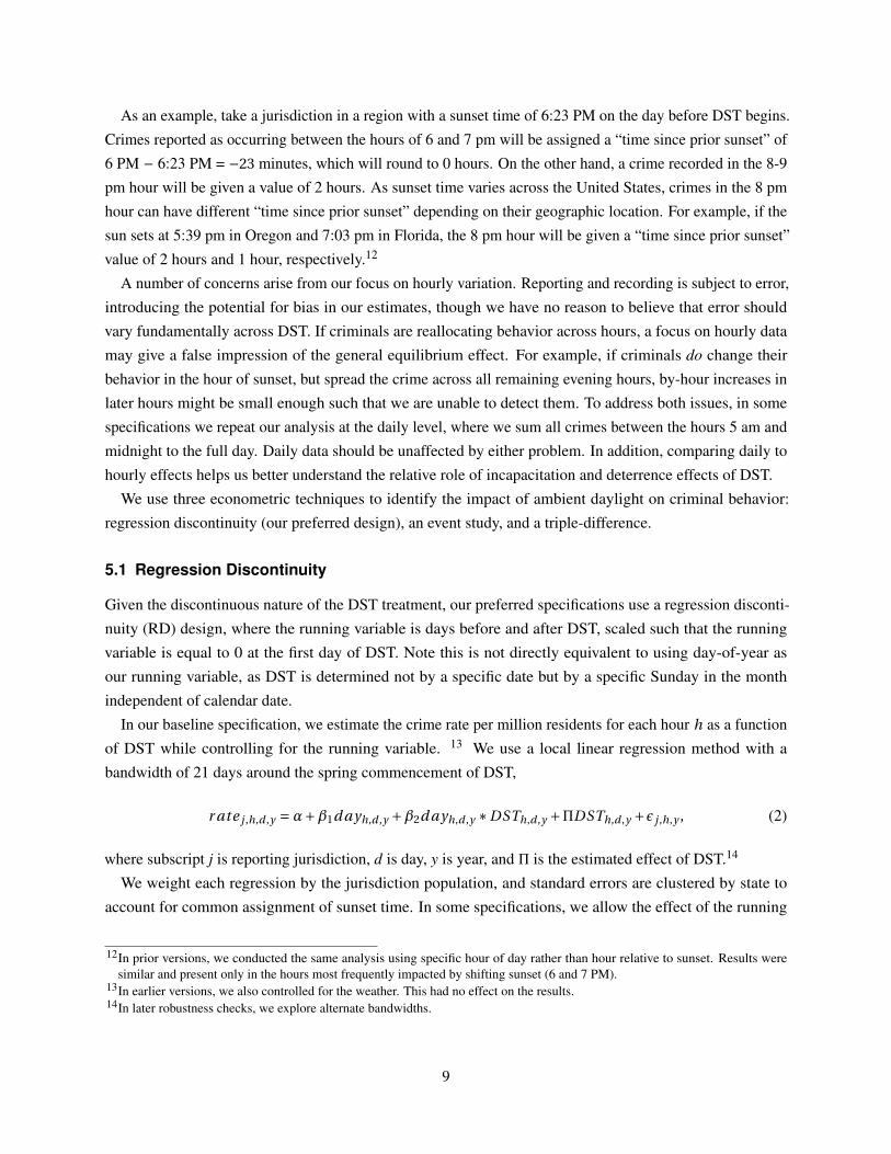
As an example, take a jurisdiction in a region with a sunset time of 6:23 PM on the day before DST begins.

Crimes reported as occurring between the hours of 6 and 7 pm will be assigned a “time since prior sunset” of

6 PM − 6:23 PM = −23 minutes, which will round to 0 hours. On the other hand, a crime recorded in the 8-9

pm hour will be given a value of 2 hours. As sunset time varies across the United States, crimes in the 8 pm

hour can have different “time since prior sunset” depending on their geographic location. For example, if the

sun sets at 5:39 pm in Oregon and 7:03 pm in Florida, the 8 pm hour will be given a “time since prior sunset”

value of 2 hours and 1 hour, respectively.12

A number of concerns arise from our focus on hourly variation. Reporting and recording is subject to error,

introducing the potential for bias in our estimates, though we have no reason to believe that error should

vary fundamentally across DST. If criminals are reallocating behavior across hours, a focus on hourly data

may give a false impression of the general equilibrium effect. For example, if criminals do change their

behavior in the hour of sunset, but spread the crime across all remaining evening hours, by-hour increases in

later hours might be small enough such that we are unable to detect them. To address both issues, in some

specifications we repeat our analysis at the daily level, where we sum all crimes between the hours 5 am and

midnight to the full day. Daily data should be unaffected by either problem. In addition, comparing daily to

hourly effects helps us better understand the relative role of incapacitation and deterrence effects of DST.

We use three econometric techniques to identify the impact of ambient daylight on criminal behavior:

regression discontinuity (our preferred design), an event study, and a triple-difference.

5.1 Regression Discontinuity

Given the discontinuous nature of the DST treatment, our preferred specifications use a regression disconti-

nuity (RD) design, where the running variable is days before and after DST, scaled such that the running

variable is equal to 0 at the first day of DST. Note this is not directly equivalent to using day-of-year as

our running variable, as DST is determined not by a specific date but by a specific Sunday in the month

independent of calendar date.

In our baseline specification, we estimate the crime rate per million residents for each hour h as a function

of DST while controlling for the running variable. 13 We use a local linear regression method with a

bandwidth of 21 days around the spring commencement of DST,

r ate j ,h,d ,y =α+β1d ayh,d ,y +β2d ayh,d ,y ∗DSTh,d ,y +ΠDSTh,d ,y +ε j ,h,y , (2)

where subscript j is reporting jurisdiction, d is day, y is year, and Π is the estimated effect of DST.14

We weight each regression by the jurisdiction population, and standard errors are clustered by state to

account for common assignment of sunset time. In some specifications, we allow the effect of the running

12In prior versions, we conducted the same analysis using specific hour of day rather than hour relative to sunset. Results weresimilar and present only in the hours most frequently impacted by shifting sunset (6 and 7 PM).

13In earlier versions, we also controlled for the weather. This had no effect on the results.14In later robustness checks, we explore alternate bandwidths.

9

variable to vary by year by interacting β1 and β2 with reporting year indicators, as crime patterns may have

changed over time. We also repeat this analysis using daily totals.

5.2 Event Study

Conditional on unobservables being smooth through the cutoff, the RD model allows for a simple, parsimo-

nious design. However, an assumption of the model is that the expected value of the outcome is the same

approaching from either side of the discontinuity cutoff. In this case, that may not be true: DST always begins

on a Sunday, and crime rate trends approaching Saturdays may be fundamentally different from Sundays in

terms of crime rates during certain hours.

As an alternate method, we use an event study. This allows us to control for day-of-week fixed effects, as

well as flexible trends in day-of-year — here we add up to a fourth-order polynomial as our main specification

(results are similar using other orders and are available upon request). We allow trends to vary across years

by interacting the polynomial with year fixed effects, now including a wider span of data (from February

through May). Finally, we allow for differential annual crime baselines by time and area by including

jurisdiction-by-year fixed effects. The event study equation is then,

r ate j ,h,d ,y =α+γy ∗ f (day of year)+Θ∗DSTh,d ,y +φ j ,h,d ,y +ε j ,h,y , (3)

As with the RD estimates, we perform this on both the hourly and daily level, weight by population, and

cluster our standard errors at the state level.

5.3 Triple Difference Estimates

DST divides weeks into pre- and post-DST groups, while the hour of sunset divides observations into

"impacted by DST vs. not". Additionally, we hypothesize certain crimes will be more drastically impacted

by changes in ambient light. We use all three sources of variation as a basis for a difference-in-difference-

in-difference strategy. This serves as a verification of our prior results and allows for the inclusion of more

flexible time effects.

We first aggregate all results to weekly averages by summing to a weekly total (where week is defined as

Sunday through Saturday). Given the relaxation of the validity of RD around the cutoff, we again expand our

timeframe to include February through May. We limit the analysis to hour of sunset (hour 0) and, as a control,

3 hours since sunset (calculated as discussed above), a time sufficiently far away from sunset that it should not

be impacted by DST. We then expand the data to be one observation per crime-by-week-by-year-by-treatment

hour cell. Given the potentially different baseline occurrence levels by crime, for the triple-difference analysis

we examine outcomes in a percentage-change framework by taking the inverse hyperbolic sine, which closely

approximates the logarithmic function but is defined for 0 values, and all our estimates can be interpreted as

percentage changes.

10

The triple-difference regression includes: (1) week-of-year fixed effects, (2) an indicator for DST which

allows the mean overall robbery rate to vary across DST, (3) an indicator for the hours with relevant daylight

impacted by DST (hour 0) which allows a consistent difference in baseline crime rates by hour, and (4) the

interaction between the indicators in (2) and (3), which is the difference-in-difference estimate impact of DST

on robbery in the relevant sunset hours. An additional difference comes with the inclusion of a counterfactual

crime in the analysis to control for broader trends in crime or police activity. The estimate of interest is now

the difference-in-difference-in-difference impact of DST (allowing for changes across both DST and the

impacted DST hours which are common among both crimes):

i nvhy psi ne(r atec, j ,h,w,y ) =α+β1weeko f yearw,y +θ1DSTw,y

+θ2r elevanthourh +θ3i mpactedc +θ4noti mpactedc

+θ5r elevanthour X i mpactedh,c +θ6r elevanthour X noti mpactedh,c

+θ7DST X i mpactedc,w +θ8DST X noti mpactedc,w

+ΠDST X r el evant X i mpactedc, j ,h,w,y +εc, j ,h,w,y , (4)

where c indicates crime, i mpacted is the crime we hypothesize to be sensitive to ambient light, and

noti mpacted is the control crime. We again weight all regressions by population and cluster all standard

errors by state. We limit this analysis to the impacted crime of robbery, as both rape and murder are very

infrequently observed. We repeat regressions using (4) four times with different control crimes in each —

forgery, swindling, shoplifting, and burglary.

6 Results

6.1 Regression Discontinuity

Table 2 shows results for our preferred specification of a regression discontinuity design. We begin by

estimating equation 2 by hour relative to sunset pre-DST as described in the beginning of Section 5, using the

crime rate per million individuals as our outcome variable. Using our robbery outcome, Figure 4 provides an

example of these results graphically showing the estimated coefficient and the corresponding 95% confidence

interval for each estimation by hour. DST has a statistically and economically significant negative effect on

the rate of reported robberies, but only in the hour most impacted by the policy in terms of ambient daylight

change (hour 0). This implies that effects are tied to DST rather than other potentially changing factors

around the same time, and that the deterrence effect is a major factor. The hour directly following sunset (1)

appears to have residual negative effect as well, which could be due to how hours since sunset is defined.

Moving sunset out of hour 0 decreases the robbery rate by 0.067 per million. Though this number may seem

small in absolute effect, the mean robbery rate during that hour on the same day of the week prior is just 0.13

per million, meaning the beginning of DST is associated with a decrease of over 51% of the prior week’s

mean.

11

Figure 5 shows the estimated local linear estimate for hour 0, again using robbery as an example. Points

are the average robbery rate per million residents for each day, weighted by population. The fitted line is

obtained by local linear regression with a bandwidth of 21 days as in the main regressions, also population

weighted. The discontinuous break is clear, and appears independent of any pre- or post-trends. Figure A-4

in the Appendix shows similar results for 2 hours before, 1 hour before, 1 hour after, and 2 hours after sunset.

As with the result of Table 2, there is a small discontinuity in the hour directly following sunset, which fits

with the hypothesis that it is hours that used to be dark but are now less so where we see changes, but little

effect elsewhere.

Based on the above results, the effect of DST on robbery is largely limited to the hour most effected by

DST. This suggests criminals are not “putting off” crimes until later in the evening when it is again dark, or

we would see positive effects in the later hours. Of course, if criminals are reallocating across the day but

doing so evenly across hours, a per-hour effect could be small enough that we are unable to detect it in our

data. To test for such effects, we repeat the RD analysis at the daily level by aggregating to daily totals as

described in Section 5. The result is shown in column 8 of Table 2. Daily totals show DST lowered robbery

rates by 0.245 per million. Based on a prior week daily mean of 1.684 per million, this suggests a daily

overall drop in robbery rates of approximately 15%.

Note that the drop in robbery over the course of the day is larger than just the drop during the treated hour.

This suggests DST has some non-zero incapacitation effect: some offenders continue to commit robbery

during the treated hour, and because it is now light outside they are more likely to get caught (our additional

finding that arrest rates for solved robberies increase with DST, which we discuss in more detail below,

supports this as well). Once in jail, they can no longer commit crime at any time of day. The deterrent

effect of ambient light, however, should only operate during the treated hour. Our treated hour effect is

approximately one-third of the total daily effect, which suggests the deterrent effect is large.

There remains the concern that some factor correlated with DST but unrelated to light might influence

our findings. Perhaps criminals are more likely to spend time with their families eating dinner out after

DST, or otherwise substitute away from criminal activity for leisure. This would still have interesting policy

implications and are part of the net effect, but in such situations we are unable to draw parallels to the role of

general lighting and probability of capture. Less interesting would be if victims simply changed when they

reported crimes, or police departments changed when they register complaints.

In order to test if such other factors exist, we consider a variety of crimes other than robbery. Our hypothesis

is as follows: if criminals respond to the increased probability of capture and/or identification, we should

see impacts only on crimes where outdoor light might influence such outcomes. We consider shoplifting,

rape, murder, aggravated assault, and motor vehicle theft as additional crimes where identification and/or

recognition remains a concern for criminals. As zero-tests, we also consider forgery and swindling, neither

of which is aided by the “cover of darkness”. Finally, we also address burglary. If DST makes individuals

remain out and away from home longer, we might expect burglary rates to increase, which would be of policy

relevance.

Negative effects are present for shoplifting, rape, and murder, and almost all effects are only in the hour of

12

prior sunset. We see no effects for motor vehicle theft, swindling, or forgery, and no statistically significant

changes in burglary. We do find one statistically significant increase in aggravated assault, but the relative

effect is small and not in an hour not consistent with an effect of DST. Of course, one danger of running so

many regressions (different crimes, multiple hours) is that, given enough subsamples, some results will arise

as statistically significant simply by chance.

Taken as a whole, results support our hypothesis that effects are driven by criminal response to probability

of identification and capture. The findings on rape and murder are of particular social importance, given the

substantial social damages of such crimes. As with the robbery results, in column 8 we show estimates done

at the daily level. While they are largely consistent with our hourly findings, results for murder are no longer

present. The effects on rape remain large and negative, but are now marginally statistically significant.

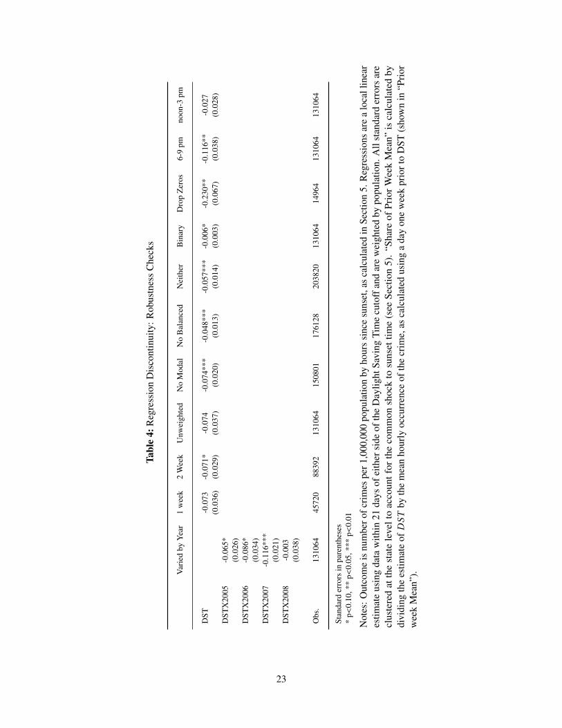
Before moving on to alternate specification techniques, Table 4 shows various robustness checks of our

RD findings with respect to a number of different model choices. For simplicity, we focus on robbery effect

in hour 0. In column 1, we allow both the effect of the running variable and the effect of DST to vary by

year. While all results are negative, findings are smaller and statistically insignificant for 2006 and 2008. In

columns 2 and 3, we restrict the bandwidth to 1 and 2 weeks on either side of DST, respectively. Column 4

repeats the main analysis without weighting. Columns 5, 6, and 7 relax our data cleaning of modal reported

hour, a balanced panel, and both combined. In all cases, results are effectively unchanged. Column 8 repeats

our analysis treating crime as a binary variable — either at least one crime occurred or no crimes occurred.

This helps control for potential outliers (e.g., unusually high crime days) driving our result. We still find

statistically significant effects, which suggest DST decreases the probability of any robbery occurring in the

sunset hour by 0.65 percentage points.15

Column 9 omits all region/year combinations in which there were no robberies. Not surprisingly, this

increases the estimated effect to 0.23 robberies per million. Finally, in columns 10 and 11, we collapse data to

four-hour windows to better address measurement error: 6-9 pm and noon-3 pm, respectively. We find large

effects for the evening hours, and no effects for the afternoon, further suggesting that our earlier results are

not the product of reporting timing and/or other changes in reporting behavior. In Table A-1 in the Appendix,

we repeat this analysis, breaking the entire day into three-hour blocks, and find results are again most present

during sunset.

6.2 Event Study and DDD

We next estimate the effect of DST using the event study model described in equation 3 for all crimes

addressed above. Table 5 shows results for the hour of sunset (panel A) and daily totals (panel B). For

robbery (column 1) results are similar to our RD findings — even with the inclusion of day of week fixed

effects and more flexible, longer-run time controls, the estimate is a reduction of 0.057 robberies per million,

within a standard error of our RD estimates. We again find results for shoplifting and rape as well. For daily

15In prior versions we modeled our results as a count model, using Poisson analysis. Results were still statistically and economicallysignificant, and effectively similar.

13

estimates, results are similar but smaller across all crimes than our RD estimates. Swindling and burglary

appear to experience some change as well, though both results are only marginally statistically significant

(p-values of 0.09 for both), and may be a further indication of an incapacitation effect if certain crimes are

compliments. Given the general consistency of our results, this suggests our findings are not overly sensitive

to the assumptions of the RD design.

Finally, we estimate a difference-in-difference-in-difference model at the weekly level. Here, identification

comes from the shifting in weeks within the year that result from the 2007 legislation. This also allows for

much more flexible time controls, where we can now include week-of-year fixed effects. Table 6 contains

our results. Column 1 shows results using forgery as the counterfactual crime, and column 2 uses swindling.

While these are both good examples of crime where darkness provides no aid, they may not be the crimes

that robbers also commit. As such, in column 3 we use shoplifting, and in column 4 we use burglary, which

may be more similar.

The coefficient of interest, the triple-interaction between indicators for relevant hour, relevant crime, and

DST, is of similar magnitude and again highly significant in all specifications — recall that RD estimates

yielded a change around 50% of the prior week mean, while estimates here range from 39% to 54% depending

on the control crime.

6.3 Further Expansions

As noted in Section 2, in each year there are two shifts in daylight caused by DST: one in the spring, and one

in the fall. Thus far, we have focused on the change that occurred in the spring. We do so for two reasons.

First, the legislative change in the spring resulted in a three-week shift in the start of DST, while in the fall

the extension only moved the end of DST a single week. Second, the end of DST corresponds very closely to

Halloween (October 31st), a date on which criminal behavior may be abnormal. Regardless, we do perform

our analysis using data from fall as a check to verify our findings. Table 7 shows these results by crime, which

are largely consistent with our spring findings. We also see statistically significant increases in shoplifting,

and burglary, which we strongly suspect are due to the presence of Halloween.

In Table 8, we consider crimes classified as “attempted” for both robbery and swindling, where an attempted

crime is defined as intending but failing to commit that crime. We focus here on robbery, shoplifting, and

rape, the crimes for which we see the most robust results. Columns 1, 3, and 5 illustrate the effect for only

attempted crimes, while columns 2, 4, and 6 use both attempted and “successful” crimes combined. A priori,

the expected size and sign of the attempted effect is not obvious — if, for example, additional daylight leads

to more crimes being disrupted, a decrease in robberies could result in an increase in attempted robberies as

individuals who would have succeeded now fail. For shoplifting, we see some changes in attempted crimes.

For both robbery and rape, however, results are negative but not significant.

We next consider how the probability of arrest varies with DST both overall and in hour 0 in Table 9.

Our outcome of interest is the fraction of crimes that result in arrest, which ranges between 0 and 1. As

this requires an observed crime, the sample size is much smaller. In the hour of sunset, there are large

14

effects for robbery, where DST results in an 11 percentage-point increase in the probability of an arrest being

made. Similar sized effects occur for rape, though results are noisy, which is not surprising given the total

observations is down to 199. Oddly, we do find a significant decrease in the number of solved shoplifting

crimes over the entire day.

As an example of how DST might impact arrest trends, Figure 6 plots the mean arrest rate for robbery in

the weeks leading up to and following DST for the hour of sunset. It appears there is a slight jump around

DST. We note, however, that a number of factors could cause this result. For example, getting caught could

be more likely, and criminals may be responding rationally by avoiding criminal behavior at this time. It may

also be a change in the criminal population, where some criminals decrease their activity after DST and some

do not, and those that remain are worse at avoiding capture.

Finally, we consider the impact of DST on crime in the early hours of the day. Our hypothesis is that,

given when criminals are active and/or individuals are out and about as potential targets, adding an additional

hour of darkness in the morning will have little effect on crimes such as robbery. Figure 7 shows that, for

hours from -2 hours before to 2 hours after sunrise prior to DST (calculated similarly to hours from sunset),

there is no effect. A specific early morning concern, raised by the Parent Teacher Association, is that children

waiting for buses in the early morning hours (which are now more likely to be dark) are more at risk for

kidnapping. To check for this effect, we also use kidnapping per million population as the outcome. Figure 8

shows no statistically significant effects. Finally, we also consider rape, as early morning hours are often

used for jogging, increasing the availability of potential victims. Interestingly, we find negative effects there

as well. The morning effect is likely due to the decrease in foot traffic (for instance, women who might have

gone running outside in the morning might go to they gym instead). In other words, we suspect the decrease

in crime comes from an increase in D(L) in the morning.

7 Discussion

We find DST lowers the overall robbery rate, and that the effect is more one of deterrence than incapacitation.

Our data further suggest the rate at which reported crimes are solved increases after DST begins. This implies

those who offend despite the daylight are (as expected) more likely to get caught —- it appears potential

offenders react to the higher probability of getting caught (and the higher expected cost of crime) by not

offending. We also find statistically and economically significant decreases in the rape rate, during both the

treated morning and evening hours.

Who benefits from this decrease in crime? Figures 9 through 11 show demographics of victims from

reported crimes during the four hours after sunset, before and after DST. DST appears to have no effect on

robberies involving black victims during the evening hours. However, it reduces the number of robberies

involving white victims during hours 0–2, while increasing them slightly in hour 3. Robberies fall for both

genders during hour 0 after DST, and increase slightly for both genders during hour 3. They fall for victims

of most ages during hour 0, but increase particularly for victims in their 20s during hour 3. These graphs

jointly suggest, to the extent that there is any increase in later-evening crime after DST, it particularly impacts

15

young adults. 16

Ideally, our results would generalize to the benefits of any ambient lighting, which includes street lights.

However, as noted above, alternative explanations for our observed effect make it difficult to fully extend

our result from the effect of DST to a general impact of an increase in ambient lighting. DST might carry

an increase in foot traffic at key times due to the later sunset, which might increase the number of potential

witnesses in addition to increasing visibility. The general equilibrium effect also may increase the number

of potential victims. If the “prime time” for crime is when most people are on their way home after work,

changes in offenders’ schedules due to the later sunset (later family dinners or sports practices, substitution

for their own leisure, etc.) might make them unavailable to commit crime until after most potential victims

have gone home. The first explanation implies DST has a deterrent effect on crime, but through an alternate

channel; the second explanation implies an incapacitation effect that does not rely on incarceration. In both

cases, generalization to the effect of any ambient light versus specifically an hour of shifted daylight is more

difficult, and our results should be interpreted with this in mind.

There remains the specific valuation of the social benefits of the decreased crime seen as a result of DST.

McCollister, French, and Fang (2010) estimates the social cost of an individual being robbed at $42,310.17

Considering only violent crimes, a back-of-the-envelope calculation implies that the three-week extension

of DST avoids $18.5 million nationally each year in avoided robberies. We also find a decrease in 0.008

murders per million population. With a social cost of murder at $8,982,907, this yields an additional avoided

cost of $468 million. Finally, the decrease in rape, with a social cost of $240,776 per occurrence, results in

an avoided cost of $71 million. Based on the number of violent crimes avoided, our calculations suggest

the 3-week spring shift in DST resulted in a total savings of approximately $558 million.18 These savings

are from the three-week period of DST extension; if we assume linear effects in other months, the implied

social savings from a permanent, year-long change in ambient light would be almost 20 times higher. We

note, however, that general equilibrium effects are likely to vary substantially across different seasons and

geographic regions, so out-of-sample prediction should be done with caution.

These avoided costs, along with the potential health benefits found in Wolff and Makino (2012), must be

compared with cost increases associated with DST. In addition to potentially increasing energy consumption,

DST appears to have several other negative consequences. A 2012 poll by Rasmussen Reports found

16It is possible the observed effect on reported crime is due to a change in reporting, not the actual number of crimes committed. Ifcriminals choose to commit crime later at night (after the sun has set), and people out later are less likely to report a crime (e.g.,drunken bar patrons versus commuters), DST could decrease the share of robberies reported without affecting the actual numberof robberies that occurred. Since unreported crimes are, by definition, unobserved, we are not able to investigate this possibility.

17The social costs of crime include estimated tangible and intangible costs. McCollister, French, and Fang (2010) divide theseinto four categories: (1) direct economic losses suffered by the crime victim, including medical care costs, lost earnings, andproperty loss/damage; (2) local, state, and federal government funds spent on police protection, legal and adjudication services,and corrections programs, including incarceration; (3) opportunity costs associated with the criminalÕs choice to engage in illegalrather than legal and productive activities; and (4) indirect losses suffered by crime victims, including pain and suffering, decreasedquality of life, and psychological distress.

18These calculations are based on an estimated reduction in crimes per 1,000,000 residents per hour, 21 days of DST, and aUS population of approximately 310 million. For robberies, for example, the number of robberies prevented each year is:0.067*21*(310,000,000/1,000,000) = 436, with similar calculations for rape and murder crimes.

16

only 45% of Americans think DST is “worth the hassle,” and remembering to change one’s clocks—and

occasionally being early or late for appointments—is inconvenient (Rasmussen, 2012). Groups consistently

lobbying against DST extensions include the national Parent Teacher Association (PTA) due to the increased

kidnapping concerns discussed earlier, and the airline industry, as changing flight schedules is costly — the

Air Transport Association estimated that the 2007 extension would cost airlines $147 million (Koch, 2005).

A growing literature on the negative effect of early school start times on academic performance suggests

that extending DST could negatively affect students by making classes earlier relative to sunrise (Wong,

2012).19 Medical research on circadian rhythms suggests shifts in the sleep cycle can have negative impacts

on response time and cognition, and on the Monday following DST, there is higher observed rate of traffic

accidents, workplace injuries, and heart attacks (Coren, 1996; Varughese and Allen, 2001; Barnes and Wagner,

2009). Janszky and Ljung (2008) note that changing one’s clocks "can disrupt chronobiologic rhythms and

influence the duration and quality of sleep" for several days, and also hypothesize negative physical effects as

a result of the policy. We note, however, most of these costs are due to the switch from Standard Time to

DST rather than the impact of a later sunset per se, and are likely small in comparison to the benefits of the

substantial drop in violent crime.

8 Conclusion

We present the first rigorous empirical estimates of the effect of ambient light on violent crime and the

decision to engage in criminal behavior. Using a legislated extension of the daylight saving time period and

the discontinuous nature of the policy as natural shocks to ambient lighting, we find an increase in light

during the hour of sunset impacts a number of socially damaging crimes, including robbery, murder, and rape,

with a total estimate social cost avoidance of over $550 million per year. We also find suggestive evidence

that much of the avoided crime comes through criminal deterrence, which means not only fewer victims but

also a lesser need for the expensive and potentially damaging incarceration process.

If street lights are a substitute for daylight, our results speak to optimal use of lighting technology as a

crime-prevention tool. While some have warned that recent decisions to turn off lights due to budget shortfalls

might lead to an increase in crime, there has so far been no credible estimate of the size of this effect. Unlike

previous work on street lights (which were not randomly placed, and likely signaled community investment),

the only treatment operating in our case is an increase in ambient light. We hope that our estimates can help

policy-makers weigh the costs and benefits of street light use more accurately. More directly, we find strong

evidence that the reduced form impact of the policy change itself was a decrease in crime, and add strong

evidence of a social benefit of extending DST to the list of previously considered potential costs. Finally, our

results further the research on the choice to engage in criminal behavior, and provide strong evidence that

policies that impact the probability of capture can have large effects on the actions of potential criminals.

19While Carrell, Maghakian, and West (2011) also consider how early classes impact school performance, their effect is independentof sunrise and thus should not be a long-term effect of DST. However, the deprivation of sleep schedules in the initial time shiftmay have its own effects.

17

References

Barnes, C. M., and D. T. Wagner (2009): “Changing to daylight saving time cuts into sleep and increasesworkplace injuries,” Journal of Applied Psychology, 94(5), 1305–1317.

Barnett, C. (2000): “The Measurement of White-Collar Crime Using Uniform Crime Reporting (UCR) Data,”FBI.

Becker, G. S. (1968): “Crime and Punishment: An Economic Approach,” Journal of Political Economy, 76,169–217.

Calandrillo, S., and D. E. Buehler (2008): “Time Well Spent: An Economic Analysis of Daylight SavingTime Legislation,” Wake Forest Law Review, 45.

Carrell, S. E., T. Maghakian, and J. E. West (2011): “A’s from Zzzz’s? The Causal Effect of School Start Timeon the Academic Achievement of Adolescents,” American Economic Journal: Economic Policy, 3, 1–22.

Coren, S. (1996): “Daylight Savings Time and Traffic Accidents,” New England Journal of Medicine, 334,924–925.

Doleac, J. L. (2012): “The effects of DNA databases on crime,” Working paper available online.

Janszky, I., and R. Ljung (2008): “Shifts to and from Daylight Saving Time and Incidence of MyocardialInfarction,” New England Journal of Medicine, 359, 1966–1968.

Kellogg, R., and H. Wolff (2008): “Daylight time and energy: Evidence from an Australian experiment,”Journal of Environmental Economics and Management, 56(3), 207–220.

Koch, W. (2005): “Daylight-saving extension draws heat over safety, cost,” USA Today, July 22.

Kotchen, M. J., and L. E. Grant (2011): “Does Daylight Saving Time Save Energy? Evidence from a NaturalExperiment in Indiana,” Review of Economics and Statistics, 93(4), 1172–1185.

Lee, D. S., and J. McCrary (2005): “Crime, Punishment and Myopia,” NBER Working Paper No. 11491.

Levitt, S. D. (2002): “Using electoral cycles in police hiring to estimate the effects of police on crime: Reply,”American Economic Review, 92(4), 1244–1250.

(2004): “Understanding why crime fell in the 1990s: Four factors that explain the decline and sixthat do not,” Journal of Economic Perspectives, 18(1), 163–190.

McCollister, K. E., M. T. French, and H. Fang (2010): “The cost of crime to society: New crime-specificestimates for policy and program evaluation,” Drug and Alcohol Dependence, 108, 98–109.

NPR (2007): “The Reasoning Behind Changing Daylight Saving,” All Things Considered, March 8.

(2010): “Facing Budget Gap, Colorado City Shuts off Lights,” All Things Considered, February 14.

(2011): “Rockford, Ill., Shuts Off Streetlights to Save Money,” All Things Considered, November 8.

Prerau, D. (2005): Seize the Daylight. Thunder’s Mouth Press.

Rasmussen (2012): “34% See Daylight Saving Time as Energy Saver,” Rasmussen Reports, March 10.

18

Van Koppen, P. J., and R. W. J. Jansen (1999): “The time to rob: variations in time of number of commercialrobberies,” Journal of Research in Crime and Delinquency, 36(1), 7–29.

Varughese, J., and R. P. Allen (2001): “Fatal accidents following changes in daylight savings time: theAmerican experience,” Sleep Medicine, 2, 31–36.

Welsh, B. P., and D. C. Farrington (2008): “Effects of Improved Street Lighting on Crime,” CampbellSystematic Reviews, 13.

Wolff, H., and M. Makino (2012): “Extending Becker’s Time Allocation Theory to Model Continuous TimeBlocks: Evidence from Daylight Saving Time,” IZA Discussion Paper 6787.

Wong, J. (2012): “Does School Start Too Early for Student Learning?,” Mimeo.

19

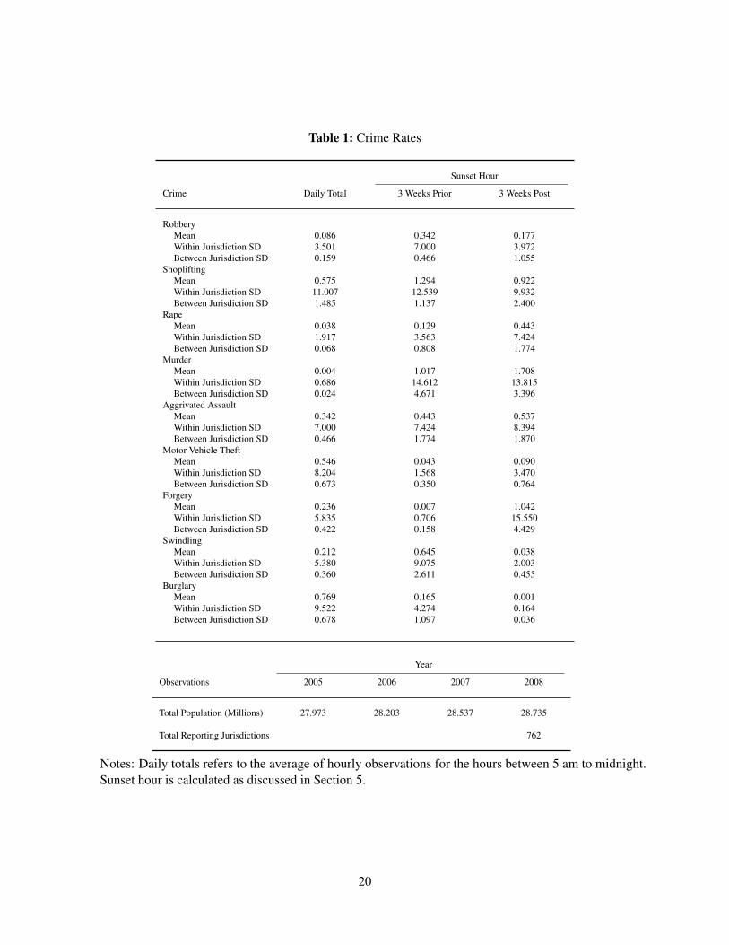
Table 1: Crime Rates

Sunset Hour

Crime Daily Total 3 Weeks Prior 3 Weeks Post

RobberyMean 0.086 0.342 0.177Within Jurisdiction SD 3.501 7.000 3.972Between Jurisdiction SD 0.159 0.466 1.055

ShopliftingMean 0.575 1.294 0.922Within Jurisdiction SD 11.007 12.539 9.932Between Jurisdiction SD 1.485 1.137 2.400

RapeMean 0.038 0.129 0.443Within Jurisdiction SD 1.917 3.563 7.424Between Jurisdiction SD 0.068 0.808 1.774

MurderMean 0.004 1.017 1.708Within Jurisdiction SD 0.686 14.612 13.815Between Jurisdiction SD 0.024 4.671 3.396

Aggrivated AssaultMean 0.342 0.443 0.537Within Jurisdiction SD 7.000 7.424 8.394Between Jurisdiction SD 0.466 1.774 1.870

Motor Vehicle TheftMean 0.546 0.043 0.090Within Jurisdiction SD 8.204 1.568 3.470Between Jurisdiction SD 0.673 0.350 0.764

ForgeryMean 0.236 0.007 1.042Within Jurisdiction SD 5.835 0.706 15.550Between Jurisdiction SD 0.422 0.158 4.429

SwindlingMean 0.212 0.645 0.038Within Jurisdiction SD 5.380 9.075 2.003Between Jurisdiction SD 0.360 2.611 0.455

BurglaryMean 0.769 0.165 0.001Within Jurisdiction SD 9.522 4.274 0.164Between Jurisdiction SD 0.678 1.097 0.036

Year

Observations 2005 2006 2007 2008

Total Population (Millions) 27.973 28.203 28.537 28.735

Total Reporting Jurisdictions 762

Notes: Daily totals refers to the average of hourly observations for the hours between 5 am to midnight.Sunset hour is calculated as discussed in Section 5.

20

Table 2: Regression Discontinuity Estimate of Impact of DST on Various Crimes, by Hours Since Sunset

Hours to Sunset Daily Total

-3 -2 -1 0 1 2 3

RobberyDST –0.015 -0.003 0.025 -0.067*** -0.033 -0.032 0.003 -0.245***

(0.019) (0.013) (0.022) (0.019) (0.035) (0.021) (0.032) (0.065)

Prior Week Mean 0.06 0.04 0.03 0.13 0.17 0.17 0.19Share of Prior Week Mean -0.25 -0.06 0.93 -0.51 -0.20 -0.19 0.02

ShopliftingDST -0.146** -0.063 -0.045 -0.201*** -0.049 -0.082* -0.040* -1.193***

(0.064) (0.051) (0.063) (0.039) (0.044) (0.042) (0.021) (0.191)

Prior Week Mean 0.74 0.82 0.66 0.48 0.36 0.19 0.19Share of Prior Week Mean -0.20 -0.08 -0.07 -0.42 -0.14 -0.44 -0.21

RapeDST -0.017 -0.002 -0.017 -0.045*** 0.013 -0.008 0.012 -0.132*

(0.012) (0.012) (0.011) (0.013) (0.015) (0.011) (0.017) (0.067)

Prior Week Mean 0.04 0.04 0.03 0.08 0.03 0.03 0.04Share of Prior Week Mean -0.39 -0.04 -0.64 -0.56 0.51 -0.29 0.28

MurderDST 0.004 -0.002 0.002 -0.008** -0.002 0.004 -0.004 0.004

(0.003) (0.003) (0.004) (0.004) (0.002) (0.005) (0.002) (0.023)

Prior Week Mean 0.00 0.02 0.01 0.02 0.00 0.00 0.02Share of Prior Week Mean . -0.12 0.27 -0.43 . . -0.22

Aggravated AssaultDST 0.023 -0.027 0.054** 0.037 0.064 0.015 0.053 0.553

(0.042) (0.031) (0.022) (0.047) (0.055) (0.028) (0.031) (0.370)

Prior Week Mean 0.29 0.41 0.40 0.51 0.47 0.41 0.41Share of Prior Week Mean 0.08 -0.06 0.14 0.07 0.14 0.04 0.13

Motor Vehicle TheftDST -0.002 0.018 -0.045 0.029 -0.076 0.009 0.018 0.177

(0.037) (0.041) (0.035) (0.042) (0.051) (0.068) (0.054) (0.238)

Prior Week Mean 0.44 0.46 0.56 0.53 0.64 0.70 0.71Share of Prior Week Mean -0.01 0.04 -0.08 0.06 -0.12 0.01 0.02

BurglaryDST 0.113* -0.052 -0.054 0.038 -0.058 -0.068 -0.051 -0.651

(0.064) (0.056) (0.063) (0.036) (0.045) (0.042) (0.036) (0.407)

Prior Week Mean 0.58 0.72 0.90 0.65 0.63 0.66 0.52Share of Prior Week Mean 0.19 -0.07 -0.06 0.06 -0.09 -0.10 -0.10

Standard errors in parentheses* p<0.10, ** p<0.05, *** p<0.01

Notes: Outcome is number of crimes per 1,000,000 population by hours since sunset, as calculated inSection 5. Regressions are a local linear estimate using data within 21 days of either side of the DaylightSaving Time cutoff and are weighted by population. All standard errors are clustered at the state level toaccount for the common shock to sunset time (see Section 5). “Share of mean” is calculated by dividingthe estimate of DST by the mean hourly occurrence of the crime, as calculated using a day one week priorto DST.

21

Table 3: Regression Discontinuity Estimate of Impact of DST on Placebo Crimes, by Hours Since Sunset

Hours to Sunset Daily Total

-3 -2 -1 0 1 2 3

ForgeryDST -0.027 -0.015 -0.006 0.025 0.023 0.001 0.026** -0.201*

(0.019) (0.021) (0.024) (0.021) (0.027) (0.017) (0.011) (0.110)

Prior Week Mean 0.12 0.11 0.04 0.04 0.04 0.04 0.05Share of Prior Week Mean -0.22 -0.14 -0.17 0.56 0.52 0.02 0.48

SwindlingDST 0.000 0.010 -0.001 0.000 0.007 0.017 -0.015 -0.249

(0.027) (0.023) (0.031) (0.019) (0.032) (0.020) (0.014) (0.169)

Prior Week Mean 0.09 0.11 0.11 0.09 0.14 0.10 0.11Share of Prior Week Mean -0.01 0.08 -0.01 0.00 0.05 0.17 -0.13

Standard errors in parentheses* p<0.10, ** p<0.05, *** p<0.01

Notes: Outcome is number of crimes per 1,000,000 population by hours since sunset, as calculated inSection 5. Regressions are a local linear estimate using data within 21 days of either side of the DaylightSaving Time cutoff and are weighted by population. All standard errors are clustered at the state level toaccount for the common shock to sunset time (see Section 5). “Share of Prior Week Mean” is calculatedby dividing the estimate of DST by the mean hourly occurrence of the crime, as calculated using a dayone week prior to DST (shown in “Prior week Mean”).

22

Tabl

e4:

Reg

ress

ion

Dis

cont

inui

ty:R

obus

tnes

sC

heck

s

Var

ied

byY

ear

1w

eek

2W

eek

Unw

eigh

ted

No

Mod

alN

oB

alan

ced

Nei

ther

Bin

ary

Dro

pZ

eros

6-9

pmno

on-3

pm

DST

-0.0

73-0

.071

*-0

.074

-0.0

74**

*-0

.048

***

-0.0

57**

*-0

.006

*-0

.230

**-0

.116

**-0

.027

(0.0

36)

(0.0

29)

(0.0

37)

(0.0

20)

(0.0

13)

(0.0

14)

(0.0

03)

(0.0

67)

(0.0

38)

(0.0

28)

DST

X20

05-0

.065

*(0

.026

)D

STX

2006

-0.0

86*

(0.0

34)

DST

X20

07-0

.116

***

(0.0

21)

DST

X20

08-0

.003

(0.0

38)

Obs

.13

1064

4572

088

392

1310

6415

0801

1761

2820

3820

1310

6414

964

1310

6413

1064

Stan

dard

erro

rsin

pare

nthe

ses

*p<

0.10

,**

p<0.

05,*

**p<

0.01

Not

es:O

utco

me

isnu

mbe

rofc

rimes

per1

,000

,000

popu

latio

nby

hour

ssi

nce

suns

et,a

sca

lcul

ated

inSe

ctio

n5.

Reg

ress

ions

are

alo

call

inea

res

timat

eus

ing

data

with

in21

days

ofei

ther

side

ofth

eD

aylig

htSa

ving

Tim

ecu

toff

and

are

wei

ghte

dby

popu

latio

n.A

llst

anda

rder

rors

are

clus

tere

dat

the

stat

ele

velt

oac

coun

tfor

the

com

mon

shoc

kto

suns

ettim

e(s

eeSe

ctio

n5)

.“S

hare

ofPr

ior

Wee

kM

ean”

isca

lcul

ated

bydi

vidi

ngth

ees

timat

eof

DS

Tby

the

mea

nho

urly

occu

rren

ceof

the

crim

e,as

calc

ulat

edus

ing

ada

yon

ew

eek

prio

rto

DST

(sho

wn

in“P

rior

wee

kM

ean”

).

23

Tabl

e5:

Eve

ntSt

udy

Est

imat

eof

Impa

ctof

DST

onV

ario

usC

rim

es

Rob

bery

Shop

liftin

gR

ape

Mur

der

Agg

.Ass

ault

Veh

.The

ftFo

rger

ySw

indl

ing

Bur

glar

y

Pane

lA:H

our

0D

ST-0

.057

***

-0.0

90**

-0.0

31**

*-0

.007

0.03

30.

039

0.02

50.

010.

015

(0.0

16)

(0.0

34)

(0.0

09)

(0.0

04)

(0.0

48)

(0.0

23)

(0.0

14)

(0.0

33)

Prio

rWee

kM

ean

0.13

0.48

0.08

0.02

0.51

0.53

0.04

0.09

0.65

Shar

eof

Prio

rWee

kM

ean

-0.4

3-0

.19

-0.3

9-0

.37

0.07

0.07

0.56

0.12

0.02

Pane

lB:D

aily

DST

-0.1

32**

-0.4

94**

*-0

.099

**-0

.005

0.36

1**

0.15

8-0

.211

-0.2

57*

-0.4

07*

(0.0

57)

(0.1

18)

(0.0

38)

(0.0

16)

(0.1

45)

(0.2

05)

(0.1

26)

(0.1

45)

(0.2

32)

Prio

rWee

kM

ean

1.68

6.72

0.60

0.09

6.09

9.35

1.39

1.60

11.8

7Sh

are

ofPr

iorW

eek

Mea

n-0

.08

-0.0

7-0

.16

-0.0

50.

060.

02-0

.15

-0.1

6-0

.03

Stan

dard

erro

rsin

pare

nthe

ses

*p<

0.10

,**

p<0.

05,*

**p<

0.01

Not

es:O

utco

me

isnu

mbe

rofc

rim

espe

r1,0

00,0

00po

pula

tion

inei

ther

the

hour

sof

suns

et(P

anel

A),

asca

lcul

ated

inSe

ctio

n5,

orfo

rthe

entir

eda

yra

ngin

gfr

om5

amto

mid

nigh

t.R

egre

ssio

nsin

clud

eda

yof

wee

kef

fect

s,fo

urth

orde

rpol

ynom

ials

inda

yof

year

that

vary

byye

ar,

and

year

-by-

juri

sdic

tion

fixed

effe

cts,

and

are

wei

ghte

dby

popu

latio

n.In

clud

edda

tara

nge

from

Febr

uary

thro

ugh

June

.All

stan

dard

erro

rsar

ecl

uste

red

atth

est

ate

leve

lto

acco

untf

orth

eco

mm

onsh

ock

tosu

nset

time

(see

Sect

ion

5).“

Shar

eof

Prio

rWee

kM

ean”

isca

lcul

ated

bydi

vidi

ngth

ees

timat

eof

DS

Tby

the

mea

nho

urly

occu

rren

ceof

the

crim

e,as

calc

ulat

edus

ing

ada

yon

ew

eek

prio

rto

DST

(sho

wn

in“P

rior

wee

kM

ean”

).

24

Table 6: Difference-in-Difference-in-Difference Estimates of Impact of DST on Crime

Forgery Swindling Shoplifting Burglary

DSTXrelevantXrob -0.432*** -0.446*** -0.394** -0.535***(0. 074) (0. 074) (0. 103) (0. 127)

Standard errors in parentheses

* p<0.10, ** p<0.05, *** p<0.01

Notes: Outcome is the inverse hyperbolic sine of crime rate per 1,000,000 population, and can beinterpreted as percentage changes. Regression specification is defined in equation 4. Analysis is done bycollapsing regressions to the weekly level and allow for week-of-year fixed effects, as well as indicatorsfor hours since sunset (0 or 3), relevant crime, and all appropriate dual interactions.

25

Table 7: Regression Discontinuity Estimate of Impact of DST on Crimes Using Fall Transition

Hours to Sunset

-3 -2 -1 0 1 2 3

RobberyDST 0.011 0.015 -0.032 -0.045* -0.017 0.002 0.050

(0.012) (0.022) (0.017) (0.018) (0.021) (0.036) (0.033)

ShopliftingDST 0.089** 0.130* 0.069 0.213*** 0.143*** 0.095 0.080

(0.030) (0.054) (0.069) (0.046) (0.033) (0.047) (0.043)

RapeDST 0.000 -0.009 0.003 0.007 0.003 0.011 -0.001

(0.008) (0.010) (0.011) (0.008) (0.006) (0.010) (0.010)

MurderDST -0.007 -0.002 -0.004 -0.003 -0.005 -0.001 -0.002

(0.005) (0.003) (0.002) (0.004) (0.005) (0.005) (0.004)

Motor Vehicle TheftDST 0.013 -0.003 0.033 0.041 0.008 -0.022 0.027

(0.042) (0.035) (0.059) (0.046) (0.056) (0.049) (0.086)

ForgeryDST 0.035 0.044 0.014 0.028 0.011 -0.006 0.001

(0.026) (0.026) (0.021) (0.025) (0.017) (0.012) (0.012)

SwindlingDST 0.017 0.041** 0.005 0.029 0.003 0.003 -0.015

(0.014) (0.012) (0.019) (0.024) (0.022) (0.032) (0.014)

BurglaryDST 0.034 0.061 0.047 0.181** 0.016 -0.024 0.049

(0.055) (0.064) (0.062) (0.064) (0.037) (0.044) (0.045)

Standard errors in parentheses* p<0.10, ** p<0.05, *** p<0.01

Notes: Outcome is number of crimes per 1,000,000 population by hours since sunset, as calculated inSection 5. Regressions are a local linear estimate using data within 21 days of either side of the end ofDaylight Saving Time cutoff and are weighted by population. All standard errors are clustered at the statelevel to account for the common shock to sunset time (see Section 5). “Share of mean” is calculated bydividing the estimate of DST by the mean hourly occurrence of the crime, as calculated using a day oneweek prior to DST.

26

Table 8: Regression Discontinuity Estimate Using Attempted and Attempted and Successful Crimes

Robbery Shoplifting Rape

Attempted Total Attempted Total Attempted Total

DST -0.001 -0.069** -0.007* -0.209*** 0.000 -0.045**(0.006) (0.019) (0.003) (0.039) (0.003) (0.014)

Standard errors in parentheses

* p<0.10, ** p<0.05, *** p<0.01

Notes: Outcome is number of attempted or attempted plus successful crimes per 1,000,000 population inthe hour of sunset, as calculated in Section 5. Regressions are a local linear estimate using data within 21days of either side of the Daylight Saving Time cutoff and are weighted by population. All standard errorsare clustered at the state level to account for the common shock to sunset time (see Section 5).

27

Table 9: Regression Discontinuity Estimate of Fraction of Crimes Solved

Robbery Shoplifting Rape

Hour 0 All Hours Hour 0 All Hours Hour 0 All Hours

DST 0.109** 0.031 0.053 -0.046*** 0.099 -0.040(0.048) (0.018) (0.047) (0.012) (0.119) (0.032)

Obs 623 9920 3495 41280 199 3611

Standard errors in parentheses

* p<0.10, ** p<0.05, *** p<0.01

Notes: Outcome is fraction of crimes reported as solved for either the full day or in the hour of sunset, ascalculated in Section 5. Regressions are a local linear estimate using data within 21 days of either side ofthe Daylight Saving Time cutoff and are weighted by population. All standard errors are clustered at thestate level to account for the common shock to sunset time (see Section 5).

28

Table 10: Regression Discontinuity Estimate Using Hour of Sunrise

Hours to Sunrise

-2 -1 0 1 2

RobberyDST -0.005 -0.002 0.004 -0.016 0.002

(0.013) (0.013) (0.015) (0.013) (0.016)

RapeDST 0.016 -0.003 -0.015** 0.012* -0.017

(0.011) (0.007) (0.006) (0.007) (0.011)

KidnappingDST 0.014 -0.002 -0.005 -0.002 -0.017

(0.028) (0.020) (0.023) (0.016) (0.012)

Standard errors in parentheses

* p<0.10, ** p<0.05, *** p<0.01

Notes: Outcome is number of crimes per 1,000,000 population in the hour of sunrise, as calculated inSection 5. Regressions are a local linear estimate using data within 21 days of either side of the DaylightSaving Time cutoff and are weighted by population. All standard errors are clustered at the state level toaccount for the common shock to sunset time (see Section 5).

29

Figure 1: Reporting Regions Used in Primary Analysis

Notes: Latitude and longitude information are taken from the 2005 Law Enforcement Identifiers Crosswalk.Each point is a reporting region included in the main analysis, as described in Section 4.

30

Figure 2: Distribution of Sunset Times in the Day Before DST

02

46

8F

requen

cy

5.5 6 6.5 7 7.5Sunset Time

2005

02

46

8F

requen

cy

5.5 6 6.5 7 7.5Sunset Time

2006

02

46

8F

requen

cy

5.5 6 6.5 7 7.5Sunset Time

2007

02

46

8F

requen

cy

5.5 6 6.5 7 7.5Sunset Time

2008

Notes: Sunset times are taken from www.timeanddate.com/worldclock/sunrise.html and are calculated asdescribed in Section 4. Y-axis represents counts of different sunset times used, where jurisdictions in thesame state share the same sunset time.

31

Figure 3: Total Robberies by Day of Year In the Hours 6 and 7 pm

17

17.5

18

18.5

19

19.5

Avera

ge S

unset H

our

05

10

15

20

25

Tota

l R

obberies p

er

1,0

00,0

00 P

opula

tion

40 60 80 100 120Day of the Year

2005

17

17.5

18

18.5

19

19.5

Avera

ge S

unset H

our

05

10

15

20

25

Tota

l R

obberies p

er

1,0

00,0

00 P

opula

tion

40 60 80 100 120Day of the Year

2006

17

17.5

18

18.5

19

19.5

Avera

ge S

unset H

our

05

10

15

20

25

Tota

l R

obberies p

er

1,0

00,0

00 P

opula

tion

40 60 80 100 120Day of the Year

2007

17

17.5

18

18.5

19

19.5

Avera

ge S

unset H

our

05

10

15

20

25

Tota

l R

obberies p

er

1,0

00,0

00 P

opula

tion

40 60 80 100 120Day of the Year

2008

Notes: Sunset time is the average of all included reporting regions. Total number of robberies is the sum ofall reported events in the hours of 6 and 7 pm on a given day of the year.

32

Figure 4: Impact of DST on Robbery Rates

−.2

5−

.2−

.15

−.1

−.0

50

.05

.1.1

5.2

.25

Chan

ge

in C

rim

es p

er M

illi

on a

nd 9

5%

CI

−3 −2 −1 0 1 2 3Hours Since Pre−DST Sunset

Notes: Each point represents the result of a different local linear regression as described in the notes of Table2. Error bars are 95

33

Figure 5: Impact of DST on Robbery Rates — Local Linear Estimates

.05

.1.1

5.2

.25

Rat

e per

1,0

00,0

00

−40 −20 0 20 40Day

Notes: Scatter plot represents hour-of-sunset means by days since the start of Daylight Saving Time, weightedby population. Fitted line is a predicted value based on a local linear regression using a bandwidth of 21 days,also weighted by population. Dashed lines represent 95% confidence intervals for predicted values.

34

Figure 6: Share of Robberies Solved

.1.1

5.2

.25

.3.3

5A

ver

age

Rat

io o

f S

olv

ed C

rim

es

−10 −5 0 5 10Weeks Since DST

Notes: Plot shows the average share of robberies categorizes as “solved” by the FBI, by weeks since thebeginning of Daylight Saving Time.

35

Figure 7: Impact of DST on Robbery Rates — Sunrise

−.2

5−

.2−

.15

−.1

−.0

50

.05

.1.1

5.2

.25

Chan

ge

in C

rim

es p

er M

illi

on a

nd 9

5%

CI

−2 −1 0 1 2Hours Since Pre−DST Sunset

Notes: Each point represents the result of a different local linear regression as described in the notes of Table10. Error bars are 95

36

Figure 8: Impact of DST on Kidnapping Rates — Sunrise

−.2

5−

.2−

.15

−.1

−.0

50

.05

.1.1

5.2

.25

Chan

ge

in C

rim

es p

er M

illi

on a

nd 9

5%

CI

−2 −1 0 1 2Hours Since Pre−DST Sunset

Notes: Each point represents the result of a different local linear regression as described in the notes of Table10. Error bars are 95

37

Figure 9: Fraction of Victims Who are Black

050

100

150

200

Den

sity

0 .2 .4 .6 .8 1Share of all Robberies in Relevant Hour

Pre DST Post DST

0

050

100

150

200

Den

sity

0 .2 .4 .6 .8 1Share of all Robberies in Relevant Hour

Pre DST Post DST

1

050

100

150

200

Den

sity

0 .2 .4 .6 .8 1Share of all Robberies in Relevant Hour

Pre DST Post DST

2

050

100

150

200

Den

sity

0 .2 .4 .6 .8 1Share of all Robberies in Relevant Hour

Pre DST Post DST

3

Notes: Dates included range from 21 days before to 21 days after daylight savings time, which varies by year.Crime statistics taken from the NIBRS victims report. Such information is not available for all crimes, andas such may not be representational of the true population events. Values are 0-1 binary indicators of anyvictims being black. Individual graph titles show hours since sunset.

38

Figure 10: Fraction of Victims Who are Male

050

100

150

Den

sity

0 .2 .4 .6 .8 1Share of all Robberies in Relevant Hour

Pre DST Post DST

0

050

100

150

Den

sity

0 .2 .4 .6 .8 1Share of all Robberies in Relevant Hour

Pre DST Post DST

1

050

100

150

Den

sity

0 .2 .4 .6 .8 1Share of all Robberies in Relevant Hour

Pre DST Post DST

2

050

100

150

Den

sity

0 .2 .4 .6 .8 1Share of all Robberies in Relevant Hour

Pre DST Post DST

3

Notes: Dates included range from 21 days before to 21 days after daylight savings time, which varies by year.Crime statistics taken from the NIBRS victims report. Such information is not available for all crimes, andas such may not be representational of the true population events. Values are 0-1 binary indicators of anyvictims being male. Individual graph titles show hours since sunset.

39

Figure 11: Age of Victims by Hour Since Sunset

010

20

30

40

50

Den

sity

0 10 20 30 40 50 60 70 80 90Number of Individuals in Robbery per Relevant Hour

Pre DST Post DST

0

010

20

30

40

50

Den

sity

0 10 20 30 40 50 60 70 80 90Number of Individuals in Robbery per Relevant Hour

Pre DST Post DST

1

010

20

30

40

50

Den

sity

0 10 20 30 40 50 60 70 80 90Number of Individuals in Robbery per Relevant Hour

Pre DST Post DST

2

010

20

30

40

50

Den

sity

0 10 20 30 40 50 60 70 80 90Number of Individuals in Robbery per Relevant Hour

Pre DST Post DST

3

Notes: Dates included range from 21 days before to 21 days after daylight savings time, which varies byyear. Crime statistics taken from the NIBRS victims report. Such information is not available for all crimes,and as such may not be representational of the true population events. Values are years of age for victims.Individual graph titles show hours since sunset.

40

A Appendix

Table A-1: Impact of DST on Robbery by Three-Hour Blocks

Three-Hour Period 5 am - 7 am 8 am - 10 am 11 am - 1 pm 2 pm - 4 pm 5 pm - 7 pm 8 pm - 10 pm

DST 0.002 -0.031* -0.028 -0.038 -0.084*** -0.023(0.015) (0.017) (0.030) (0.028) (0.022) (0.047)

Standard errors in parentheses* p<0.10, ** p<0.05, *** p<0.01

Notes: Outcome is change in number of total crimes per 1,000,000 population by 3-hour blocks. Re-gressions are a local linear estimate using data within 21 days of either side of the Daylight Saving Timecutoff and are weighted by population. All standard errors are clustered at the state level to account for thecommon shock to sunset time (see Section 5). “Share of mean” is calculated by dividing the estimate ofDST by the mean hourly occurrence of the crime, as calculated using a day one week prior to DST.

41

Figure A-1: Modal Hour of Reported Crimes

0.0

5.1

.15

.2.2

5D

ensi

ty

0 5 10 15 20 25modehour

Notes: Modal hour is found by counting the total number of reported crimes, by hour, by jurisdiction. Y-axisis density of occurrence.

42

Figure A-2: Total Robberies by Day of Year In the Hours 3 and 4 pm

17

17.5

18

18.5

19

19.5

Avera

ge S

unset H

our

05

10

15

20

Tota

l R

obberies p

er

1,0

00,0

00 P

opula

tion

40 60 80 100 120Day of the Year

2005

17

17.5

18

18.5

19

19.5

Avera

ge S

unset H

our

05

10

15

20

Tota

l R

obberies p

er

1,0

00,0

00 P

opula

tion

40 60 80 100 120Day of the Year

2006

17

17.5

18

18.5

19

19.5

Avera

ge S

unset H

our

05

10

15

20

Tota

l R

obberies p

er

1,0

00,0

00 P

opula

tion

40 60 80 100 120Day of the Year

2007

17

17.5

18

18.5

19

19.5

Avera

ge S

unset H

our

05

10

15

20

Tota

l R

obberies p

er

1,0

00,0

00 P

opula

tion

40 60 80 100 120Day of the Year

2008

Notes: Sunset time is the average of all included reporting regions. Total number of robberies is the sum ofall reported events in the hours of 3 and 4 pm on a given day of the year.

43

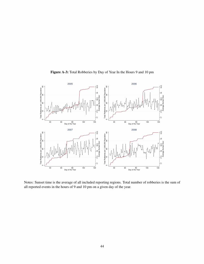
Figure A-3: Total Robberies by Day of Year In the Hours 9 and 10 pm

17

17.5

18

18.5

19

19.5

Avera

ge S

unset H

our

010

20

30

40

Tota

l R

obberies p

er

1,0

00,0

00 P

opula

tion

40 60 80 100 120Day of the Year

2005

17

17.5

18

18.5

19

19.5

Avera

ge S

unset H

our

010

20

30

40

Tota

l R

obberies p

er

1,0

00,0

00 P

opula

tion

40 60 80 100 120Day of the Year

2006

17

17.5

18

18.5

19

19.5

Avera

ge S

unset H

our

010

20

30

40

Tota

l R

obberies p

er

1,0

00,0

00 P

opula

tion

40 60 80 100 120Day of the Year

2007

17

17.5

18

18.5

19

19.5

Avera

ge S

unset H

our

010

20

30

40

Tota

l R

obberies p

er

1,0

00,0

00 P

opula

tion

40 60 80 100 120Day of the Year

2008

Notes: Sunset time is the average of all included reporting regions. Total number of robberies is the sum ofall reported events in the hours of 9 and 10 pm on a given day of the year.

44

Figure A-4: Residuals for Local Linear Estimate of Robberies in Different Hours Around Sunset

0.1

.2.3

Rat

e per

1,0

00,0

00

−40 −20 0 20 40Day

0.1

.2.3

Rat

e per

1,0

00,0

00

−40 −20 0 20 40Day

0.1

.2.3

Rat

e per

1,0

00,0

00

−40 −20 0 20 40Day

0.1

.2.3

Rat

e per

1,0

00,0

00

−40 −20 0 20 40Day

Notes: Scatter plot represents time relative to sunset means by days since the start of Daylight Saving Time,weighted by population. Fitted line is a predicted value based on a local linear regression using a bandwidthof 21 days, also weighted by population. Dashed lines represent 95% confidence intervals for predictedvalues.

45