State Income, Employment, Infrastructure and Well-Being:

Do Party Control and Political Competition Matter?

by

Oded Izraeli

Department of Economics Oakland University

Rochester, MI 4839 izraeli@oakland.edu

1-248-370-3524

Sherman Folland Department of Economics

Oakland University Rochester, MI 48309

May 2007

ii

Abstract

This paper examines the relationship between state party politics and the economic

performance of the state over six four-year periods covering the years 1978 to 2002. Novel

features include that the study examines the role of party control in a panel, it examines the

effects of political competitiveness, measures effects not only on income variables but also on

employment, tax, and spending policies, infrastructure investment, and quality of life variables.

The main finding is that control of the executive branch, the legislative branch, or both branches,

has no significant effect on state outcomes, but the degree of political competitiveness in these

data reveals significant and usually beneficial effects on employment and on quality of life

outcomes. The paper also investigates possible factors that could otherwise mistakenly account

for the negative conclusion on party control. We hypothesize that both parties, when in

competition for votes, will adopt those economic policies believed to be effective by the

politically median voter, regardless of party stereotypes, but that the competition between the

parties may provide benefits to the public by forcing politicians to sharpen their policy skills.

I. Introduction

Numerous studies address the effect of economic conditions on election outcomes.

Several focus on presidential elections (Fair, 1978; Meltzer and Vellrath, 1975; Abrams and

Settle, 1978), and others on congressional elections (Bennett and Wiseman, 1991; Zupan, 1991;

Kramer, 1971; Stigler, 1973). Other studies examine gubernatorial elections (Peltzman, 1987;

Adams and Kenny, 1989). The general approach in these cases was to associate the votes for the

incumbent party (or candidate) with economic performance, especially the immediate period

preceding the election. Intuitively, we expected that “good” economic performance rewards the

incumbent party.

Very few, however, study the question of whether it makes any difference which party is

in power, or whether political competitiveness itself has an effect on state outcomes. Regarding

the effect of party control, two exceptions are papers by Blaise, Blake and Dion (1993 and 1996).

In the first one, the authors asked "…if it matters which party forms the government.” These

authors look at the effect of party on government size, that is, how much government spends.1 In

the second, they test the effect of the party on the rate of increase in government’s spending.

Their sample consists of national governments. Winters (1976) investigated the effect of the

party on state government size. Brace (1989) raised the question as we do, “…how state

politics, however defined, might influence state economies"; his work has shown the importance

of the national markets on state performance and finds a general irrelevance of state politics and

policies. According to findings of Gilligan and Matsusaka (1995), state "political parties do not

have a pronounced effect on overall levels of expenditure, but do influence the composition of

spending" (p. 383). Levitt and Poterba (1999) investigate “…the effect of representation on an

economic outcome…” In their case they study the effect of the political party of the state

governor on welfare spending.

2

The present study focuses on the effect of party composition and political competition on

the economic outcomes of states including those intermediate state practices that can affect either

state income or the well-being of its citizens. This takes the investigation "behind the scenes" to

examine the mechanisms in comparison to the public stereotypes of the parties: Do Democrats

reduce the unemployment rate, invest more in public schooling, highways, do they raise tax

rates? Do Republicans foster a better and safer quality of life, are they more business friendly?

The advantage of using the state as the unit of observation is that it provides a sample large

enough to test several hypotheses.2 Also, the economic aspects of state elections might be more

important to individual's economic lives than national elections if only because national elections

usually are dominated by non-economic issues such as foreign policy and national security.

However, a disadvantage arises in that state governments have relatively little control of state

income performance, despite campaign rhetoric. The present framework requires that they have

at least in principle, the power to influence state outcomes. We also present evidence on the

question: Does the performance of the state economy depend to a substantial extent on

developments occurring outside the state borders, i.e., on the regional or national level.3

However, even though state governments print no money nor protect their borders against

competition from other states and countries, they still enjoy enough power in principle to have an

influence on their voters’ economic well being to some extent. Examples of policies include: 1)

the power to tax (positive and negative), 2) the decisions on what to spend budget money and

how much, 3) the borrowing of money for long-term investments, 4) the development of state

infrastructure, 5) the regulation of resources, and 6) the control over the state bureaucracy.4

According to Hansen (1999), “Since the 1970s state governors have claim to a more active role

for themselves in state economic development (p. 170).” This is not to say that the state can

determine its own economic destiny by itself. Nevertheless, the state government can control the

3

magnitude of the spillover effect from the regional and national economies to the state

economy.5 High state taxes and inefficient bureaucracy may slow down and weaken the

spillover effect of growing national economy, whereas investment in infrastructure and efficient

bureaucracy can bring more economic development to the state.

Since in almost all states, the governor’s term lasts four years,6 we will consider the

governor to be accountable for the state economic performance over a period of four to eight

years following the governor's term. These lags are chosen to allow time for the government's

policies to have effect.

The paper is organized as follows: The next section provides a background discussion of

prior empirical work. The third section describes the data and develops the empirical model. The

fourth section contains the reports of the regression estimates and the analyses. The last section

offers a summary and conclusions.

II. Background Discussion and Empirical Evidence

The competition over the control of state government takes place mainly over changes in

the representation of the two major parties: the Democratic and the Republican parties. As stated

by Morehouse (1981), “The single most important factor in state politics is the political party.”

Winters (1976) adds to this, “We define our candidates in party terms and our issues in party

terms.”7 The role political parties play in the political process according to Jones and Hudson

(1998) is to "…reduce the 'transaction costs' of electoral participation. Political parties provide a

low cost signal of the candidate's policies and personal characteristics and in this way reduce

voter's information costs (p. 175)." Greene and Nelson (1998) hypothesize that this is done

because the "…party performs as an ideological label (p. 4)." The effect of the party

composition of government on policies is the subject of several studies. Winters (1976) looks at

4

the difference between the two parties regarding the distribution of tax burden and spending

benefits. Blaise, Blake and Dion (1993 and 1996) test the effect of the party composition of

government on government size as well as the nature of the budget spending. Their findings

suggest that in a government controlled by the left, the rate of growth of spending is higher as

compared to a government controlled by the right (1996: 517). Morehouse (1981) argues that,

“It is not possible to understand the differences in the way states carry out the process of

government without understanding the type of party whose representatives are making decisions

that affect the health, education, and welfare of its citizens.” All these studies are concentrated

on the differences in policies due to the party composition of the government.

It is reasonable to expect that the two parties favor “good” economic performance, that is,

economic growth, full employment, low taxes and so on.8 On many occasions, however, it is

impossible to achieve all economic goals at the same time, so the government must choose

among the different goals. The main differences between the two parties are in the choices that

they make, that is, their differences in priorities. Hibbes (1987) suggests that the Democrats

favor a high growth rate and low unemployment and Republicans are more concerned with the

risk of inflation. Thus, "Democratic administrations are more likely than Republican ones to run

the risk of higher inflation rates in order to pursue expansive policies designed to yield lower

unemployment and extra growth (p. 218)."9 A similar view was expressed by Alesina and

Rosenthal (1995) regarding the different priorities between the two parties. It is believed that

political parties can not signal one set of priorities at the national level and a different one at the

state level. Therefore, although Hibbes' observation of the political parties' behavior was at the

federal level, it would follow that the same set of priorities is true at the state level. Thus,

throughout this study, we search for empirical evidence that the parties follow these stereotypes

at the state level.

5

But, can the null be rejected? The null hypothesis is that state party policies have no effect on

state economic performance.

There is another way, however, that state party politics can improve state economic

outcomes. Suppose that party characteristics bring the ideological faithful to the voting booth,

but the median voters are the ones who swing the election. The two parties, in this view, compete

for the center by both promising to address the same centrist priorities. It then is the mere fact of

political party competition that benefits the people of the state. Competition forces both parties to

strive to develop the genuine capabilities by which to address the need of the public.

In what follows, we develop and estimate an empirical model to address both questions:

1) Does party control matter for state economic outcomes? 2) Does the level of state political

competition influence state economic outcomes? The estimates are derived from regressions

using panel data methods. But often the simplest statistics can give a useful presaging of where

the more sophisticated approaches will lead. Table 1 reports the means of the income growth

variables separated into categories by political control during the prior eight years. These data

suggest that differences by party control are not great. They also show that much of a state's

growth rate reflects growth in its region.10

TABLE 1 ABOUT HERE

III. The Data and the Econometric Models

The data for this study are observations of the 50 states in a panel of six year's cross-

sections: 1978, 1982, 1986, 1990, 1994, and 1998.11 Economic variables—GSP, personal

income, employment, unemployment—are treated as dependent variables in regression equations

applied to test political effects on key economic outcomes, often the focus of state political

6

campaigns. As with all variables in the study, the names and extended definitions and the sources

for these variables are provided in the Appendix. Political variables include: political party of

governor, party majority in state house and senate, as well as the percentage vote for the

Democrat in the most recent presidential election. Quality of life variables include: poverty rate,

infant mortality rate, crime rate, and social capital. The social capital rating for each state is

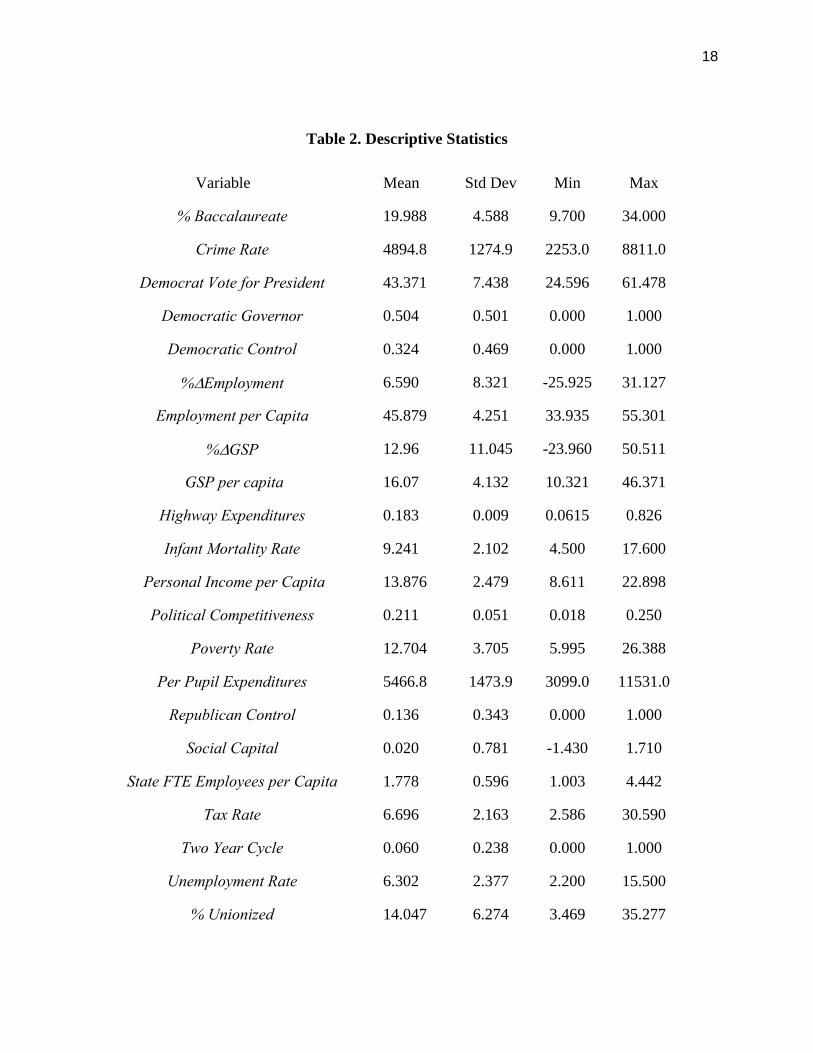
provided to this study from a paper on state health issues (Folland, 2007, 2006). Table 2 presents

the descriptive statistics for the variables.

TABLE 2 ABOUT HERE

In panel regression with fixed effects and period effects, we first apply three variables as

measures of economic performance: 1) the rate of growth of real gross state product; 2) GSP per

capita and 3) personal income per capita. Political control variables are lagged one period, giving

party effects on state outcomes needed time to bear fruit (Adams and Kenny, 1989). Some policy

effects take much longer; for example, investment in infrastructure such as highway construction

and education; in that case, we test for party effects directly on measures of investment in

highway and two education variables.

Party effects, if they exist, require the party’s control of the governorship and/or the

house and senate of the state. Several measures will be tested to explore these possibilities.

When the governorship is controlled by the Democrats, we identify a corresponding variable

(Democratic Governor) to equal one; zero when the governorship is controlled by the

Republicans. When the state house and the state senate are both controlled by a Democratic

majority, the corresponding variable (Both Houses Democrat) is set to equal one; this variable is

zero when Republicans control both houses as well as when control is split. Finally, a minority

7

of states exhibited control of all--the governorship, the state house and the state senate--by the

Democrats; these cases are identified as Democratic Control. Similar control by the Republicans

is identified as Republican Control.

As we analyze the findings, we will look for corroborating or contrasting cases vs. a vs.

popular reputations of the parties, each condensed out of perceptions of the parties in the media.

Democrats by reputation promote government spending, favor K-12 spending, support unions,

promote aid to the poor and support social freedoms. Republicans by the same media, are more

business friendly, seek to cut taxes and promote traditional social values.

Nevertheless we propose that alternative views may be more realistic. Both Democratic

and Republican parties are composed of coalitions that are sometimes at odds within the Party.

Republican advocates of free markets are often at odds with pro-business Republicans who may

have strong ties to local firms or industries. Religious and moral issue advocates among

Republicans may expend effort on policies that work to place limits on social behaviors, without

any economic payoff. Yet, political campaigns often demand that both candidates claim to

effectively address economic progress, the campaign priorities that prevail may not be the

genuine priorities for some party subgroups.

Democrats similarly collect disparate groups: industrial unions, teachers, immigrants, and

both pro-market advocates as well as globalization skeptics. Like their Republican opponents,

when billfold issues dominate a campaign, the Democrats must demonstrate that they are at least

as competent as the opposition. Since both parties compete for the same prize, and since both

parties have member groups who have interests that may conflict with economic progress, the

result may become a muddling through during which there may be little real difference between

the parties regarding genuine state economic progress.

8

We entered this research as agnostics on these possible outcomes. While previously

published articles have been negative on party effects, they have generally been focused on

limited aspects of state economic performance. We have designed tests that are more thorough in

several respects. First, we construct a panel that offers multiple looks at the 50 states. Second,

we look not only on economic progress, but also on effects on policies intermediate to economic

progress. Further, we investigate quality of life including the role of alternative theories to

political influence, that may affect a community's well being, particularly from political science

and sociology.

Regression Models

Since there is not a single most acceptable measure of the state performance we

experiment with several variables. They are: the rate of growth of real gross state product

(%ΔGSP), the rate of growth of employment (%ΔEmployment) the per capita gross state product

(GSP per Capita), the per capita real personal income (Personal Income per Capita) the state

unemployment rate (Unemployment Rate). All monetary variables were deflated by the

consumer price index.12

The independent variables include13 the political party variables. State economic

performance can be affected in principle by variables measuring political influence, and we

include these in the specification. On one hand, party power does not lie exclusively with the

governor but includes other centers of political power, especially the legislative branch. Wagner

(2001) find that the level of current spending (or saving) is influenced by members of the lower

State House with expectations regarding reelection: “The estimation results indicate that a future

change in the controlling party of a state lower house is significantly correlated with a reduction

9

in current per capita saving (p. 151)." The statistical method chosen is OLS regression analysis

with state fixed effect and period effects.

The independent variables include14 The political party variables, which have been

defined. (a complete description of all regression variables is provided in the Appendix.)

Following Levitt and Poterba, we also include a variable, Political Competitiveness, that

measures the degrees of political competition in each state. We assume that competition

increases the closer the proportion of Democrats in the House and Senate combined is to the

proportion of Republicans. Thus Political Competitiveness is measured as the product of the

percent of the vote for state house and senate taken by the Democrats times the corresponding

Republican percent of the vote. Thus this variable ranges from 0 to 0.25, and it increases as the

shares of votes become more equally distributed, hence, more competitive.

The dummy variable, TwoYear Cycle, represents the states that held their gubernatorial

election every two years. The variable, %Baccalaureate, is the education attainment level as

measured by the percent of population 25 years or older with four years of college or more. The

variable %Unionized measures the percent of workers which are members of a union. State fixed

effects and period effects were included in all cases. Potentially many state characteristics will

affect economic outcomes such as economic resources, urban/rural mix, and local culture. These

can in principle be controlled for by applying the fixed effects model in panel. We feel that not

applying the fixed effects model would lead to unreliable results.

Other variables studied in this paper include: the state Tax Rate defined as state tax

revenue as a percent of personal income. The per capita number of full time equivalent state

employees, State FTE Employees, measures the size of the government. When more state

revenue is allocated to infrastructure and human capital development it should have a positive

10

effect on the state economic performance in later years. We measure Per Pupil Expenditures, as

well as Highway Expenditures, and College expenditures by the state, these on a per capita basis.

IV. Regression Studies and Analyses

A. Income Measures

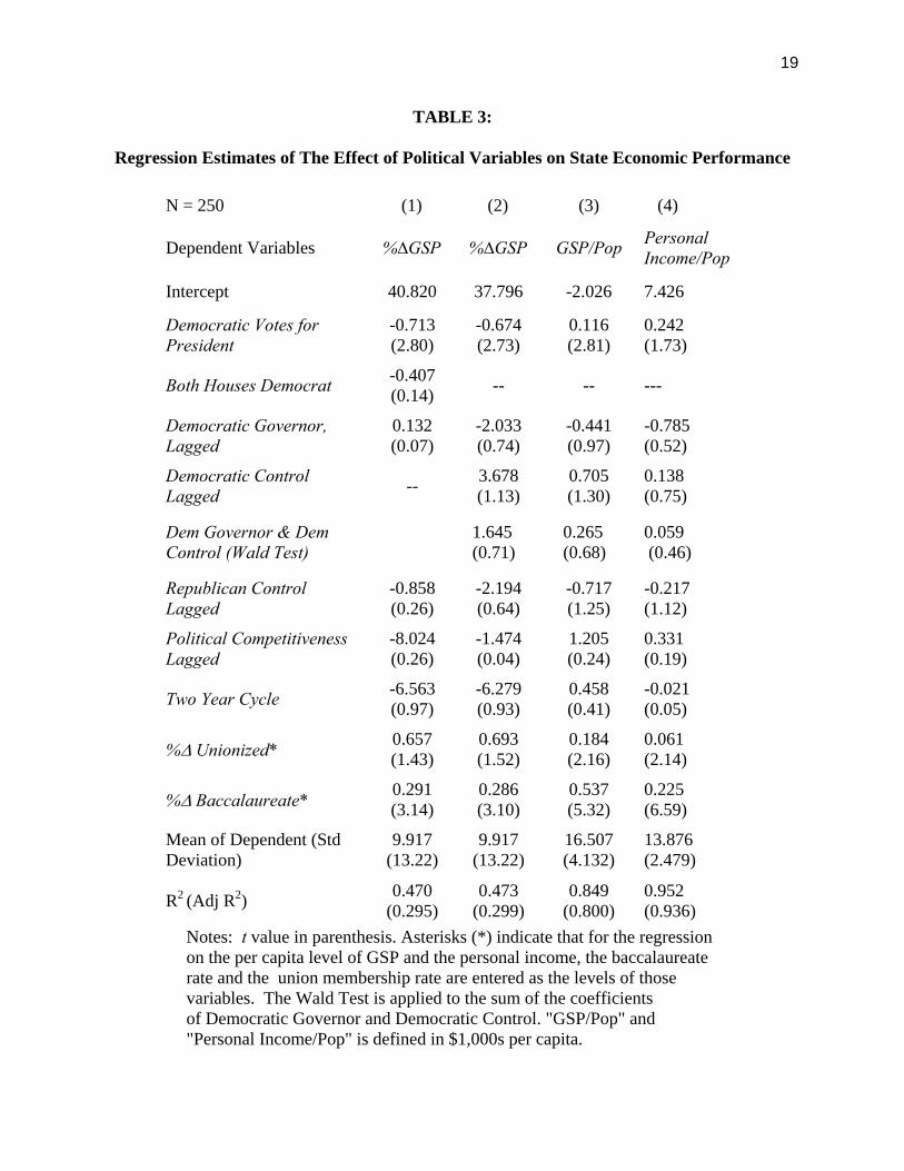
As shown in Table 3, there are no significant effects of party control on gross state or on

personal income per capita. The Democratic Governor variable tests for a distinctive role of the

governorship; since generally governors are either Democrat or Republican, the result also

suggests that having a Republican governor has no effect on state economic performance.

The Democratic Governor variable and the Democratic Control variable both measure an

aspect of Democratic influence. The inclusion of both of these Democratic variables was

intended to capture possible independent effects of Democratic Governor versus complete

Democratic Control. For example, does a governor without control of the legislature

nevertheless have a positive effect on economic growth? However, the insignificance of the

Democratic Governor variable implies that no conclusion can be drawn regarding this side

hypothesis. We tested the combined hypothesis that the sum of the two Democratic coefficients

centers on zero; the Wald Test coefficient for the sum of the two Democratic control coefficients

and the corresponding t value is given in a separate row.

Equation (1) reports an insignificant result for the variable Democratic Majority in Both

Houses. The two variables, for Democratic and Republican control, which represent instances of

one party control of both the executive branch and the legislative branch of government, also fail

to attain significance. Setting GSP per Capita as the dependent variable yields similar results.

The political variable Democratic Votes for President measures the percent of the state voters

who voted Democratic in the previous presidential election, and functions loosely as a control for

11

"red states versus blue states". The coefficients for this variable suggest that the level of income

is higher but the growth rate lower in the "blue states". The human capital measure,

%Baccalaureate, enters with the expected positive sign and significant coefficient. %Unionized

enters positively and significant or close to being significant, suggesting perhaps that organized

labor was not an impediment to economic growth.

TABLE 3 ABOUT HERE

Also please note that political competitiveness has no significant effect on income

variables. Together with lack of significance in the party control variables, these results are

consistent with the view that state political groups have achieved little or no influence over state

income growth performance.

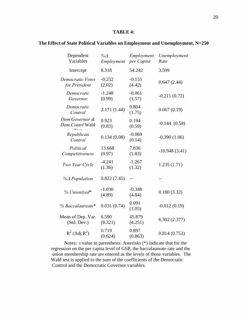
B. Employment Both the level of employment and growth in employment lag somewhat in "blue states";

see the coefficient for Democratic Votes for President in Table 4. State party control, however,

(see also the results for both Democratic controls in the Wald Test row) affects neither

employment nor unemployment. In contrast, political competition affects employment per capita

and the unemployment rate in a salutary manner, suggesting that employment per capita and the

unemployment rate both serve as a key political issue and represent cases where policy can affect

outcomes.

TABLE 4 ABOUT HERE

12

C. Taxing and Spending Previous studies on the subject, like Blaise, Blake and Dion (1993 and 1996), found that

government tends to spend more when it is controlled by a politically left party as compared to a

government which controlled by a politically right party. Following this line of thought one

might hypothesize that a state controlled by the Democrats tends to have a bigger government.

This hypothesis correlates with the political legend that Democrats are the party of "tax and

spend". But problems clearly arise with this view. Taxes fund infrastructure investment, thus

fueling economic growth, but they also pay for growing consumer tastes for public amenities.

Also it is possible that they fund government waste. The true combination of these things may be

hard to tell for any given state. Two variables here serve as measures for the size of government,

the state Tax Rate (the Tax Rate is the ratio of total state tax revenue to state personal income)

and State FTE Employees. The results reported in Table 5, however, indicate no significant

influence of the Democratic (as per the Wald Test) or Republican party on these two measures.

One does note, however, that %Unionized and %Baccalaureate do have significant coefficients,

and Political Competitiveness is significant in the state employees equation.

TABLE 5 ABOUT HERE

D. Infrastructure Investment

Investment in infrastructure, such as education and highways, reap payoffs for the state

that last well into the future, beyond the terms of office of present day state politicians. Hence,

these investments would have diminished attractiveness to politicians, at least to those politicians

whose primary goal is to get reelected. Table 6 reports no significant effects of party control or

13

competitiveness for investments in K-12 pupils, per capita investments by the state in colleges,

or highway expenditures per capita.

TABLE 6 ABOUT HERE

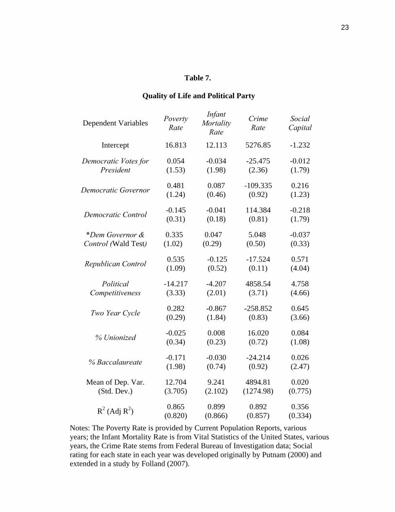
E. Quality of Life

Does party politics matter in residents’ everyday lives? Table 7 selects four indicators of

quality of life, Poverty Rate, Infant Mortality Rate, Crime Rate and Social Capital. These

indicators are well known, except perhaps for social capital. This is a variation on the Social

Capital Index developed by Robert Putnam (2000) for the year 1994 and was extended back to

1976 and made available to this study in work by Folland (2007). It represents a factor analytic

combination of survey results regarding people's views of the community, their rate of sociable

interchange, and their degree of participation in community activities. The results in Table 7

highlight the role of Political Competitiveness, which provides a significant beneficial effect in

most cases (the Crime Rate is the exception).

TABLE 6 ABOUT HERE

F. Challenging the Negative Findings The repeated finding of "no party control effect" stands out as a central message of this

study. While related similar results arise in the literature, those discoveries have been mainly the

result of more narrowly focused empiricism or even on conjecture. We searched here for an

effect in each place where one could plausibly expect to find one--state economic growth, state

personal income levels, employment, taxing and spending, infrastructure, and quality of life--and

14

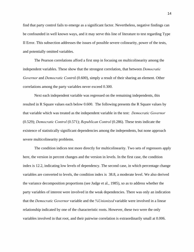
find that party control fails to emerge as a significant factor. Nevertheless, negative findings can

be confounded in well known ways, and it may serve this line of literature to test regarding Type

II Error. This subsection addresses the issues of possible severe colinearity, power of the tests,

and potentially omitted variables.

The Pearson correlations afford a first step in focusing on multicolinearity among the

independent variables. These show that the strongest correlation, that between Democratic

Governor and Democratic Control (0.600), simply a result of their sharing an element. Other

correlations among the party variables never exceed 0.300.

Next each independent variable was regressed on the remaining independents, this

resulted in R Square values each below 0.600. The following presents the R Square values by

that variable which was treated as the independent variable in the test: Democratic Governor

(0.529); Democratic Control (0.571); Republican Control (0.286). These tests indicate the

existence of statistically significant dependencies among the independents, but none approach

severe multicolinearity problems.

The condition indices test more directly for multicolinearity. Two sets of regressors apply

here, the version in percent changes and the version in levels. In the first case, the condition

index is 12.2, indicating low levels of dependency. The second case, in which percentage change

variables are converted to levels, the condition index is 38.8, a moderate level. We also derived

the variance decomposition proportions (see Judge et al., 1985), so as to address whether the

party variables of interest were involved in the weak dependencies. There was only an indication

that the Democratic Governor variable and the %Unionized variable were involved in a linear

relationship indicated by one of the characteristic roots. However, these two were the only

variables involved in that root, and their pairwise correlation is extraordinarily small at 0.006.

15

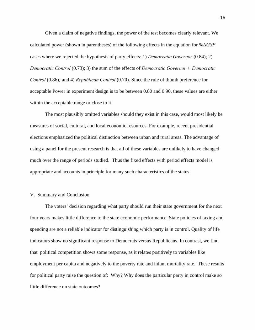
Given a claim of negative findings, the power of the test becomes clearly relevant. We

calculated power (shown in parentheses) of the following effects in the equation for %ΔGSP

cases where we rejected the hypothesis of party effects: 1) Democratic Governor (0.84); 2)

Democratic Control (0.73); 3) the sum of the effects of Democratic Governor + Democratic

Control (0.86); and 4) Republican Control (0.70). Since the rule of thumb preference for

acceptable Power in experiment design is to be between 0.80 and 0.90, these values are either

within the acceptable range or close to it.

The most plausibly omitted variables should they exist in this case, would most likely be

measures of social, cultural, and local economic resources. For example, recent presidential

elections emphasized the political distinction between urban and rural areas. The advantage of

using a panel for the present research is that all of these variables are unlikely to have changed

much over the range of periods studied. Thus the fixed effects with period effects model is

appropriate and accounts in principle for many such characteristics of the states.

V. Summary and Conclusion The voters’ decision regarding what party should run their state government for the next

four years makes little difference to the state economic performance. State policies of taxing and

spending are not a reliable indicator for distinguishing which party is in control. Quality of life

indicators show no significant response to Democrats versus Republicans. In contrast, we find

that political competition shows some response, as it relates positively to variables like

employment per capita and negatively to the poverty rate and infant mortality rate. These results

for political party raise the question of: Why? Why does the particular party in control make so

little difference on state outcomes?

16

One possible answer, of course, is that of those economists who believe that state

economic performance cannot be determined by the state government arguing that the state

government's ability to conduct an independent fiscal policy is limited by the fact that they can

not print money, and the state is an open economy with free mobility of resources. However, we

believe that the state has tools of investment and economic environment to substantially

influence its economic development. We argue instead that the economic policy of the state

depends on the choices of politicians but simply does not depend on party line. The ideologies of

the two major parties are certainly different, yet, whichever party gains power is forced to face

reality, that is, the existing perceptions of the voting public. The actual policies come to be not so

much based on the party ideology but tend to depend more on the politic and economic market

forces. In contested elections, there may not be much room to manipulate. Nevertheless it is still

possible for different groups to realize economic gains solely because their party won the

election. The coalitions of interest groups expect their party's candidate to do better for the state,

but more importantly, to improve their own well being.

A related view is that the political competition itself that is helpful. In this view,

competition hones the policy skills of both parties, but the party that survives the competition

with the voters is itself an outcome greatly affected by chance. Finally we note that neither party

control nor political competition work to improve growth in GSP, it may be that this negative

result stems from both state politicians' limited policy ability in this area of endeavor but also

from the limited tools by which any state can improve its state product.

17

Table 1. Mean State Growth Rates Over Two Political Cycles* by Political Control %Δ in %Δ personal Political control throughout %Δ in GSP income per prior eight years: GSP Net capita N

The governorship controlled by Democrats (but statehouse not)

23.72 2.10 8.98 36

Both the statehouse and the governorship controlled by Democrats

30.73 7.98 13.85 41

The governorship controlled by Republicans (But statehouse not)

28.74 9.67 10.60 37

Both the statehouse and the governorship controlled by Republicans

33.26 15.22 12.43 12

Political control mixed between the parties, governorship, statehouse and/or years

21.98 0.87 11.85 74

*Notes: These mean percentage changes are based on the changes in the variables, from eight years prior to the "present". The percentage changes for the years 1986, 1990, 1994, 1998 were then averaged. The data years 1978 and 1982 were deleted because they lacked the required lagged values. %ΔGSP Net is the percentage change in gross state product net of the mean percentage change within its region.

18

Table 2. Descriptive Statistics

Variable Mean Std Dev Min Max

% Baccalaureate 19.988 4.588 9.700 34.000

Crime Rate 4894.8 1274.9 2253.0 8811.0

Democrat Vote for President 43.371 7.438 24.596 61.478

Democratic Governor 0.504 0.501 0.000 1.000

Democratic Control 0.324 0.469 0.000 1.000

%ΔEmployment 6.590 8.321 -25.925 31.127

Employment per Capita 45.879 4.251 33.935 55.301

%ΔGSP 12.96 11.045 -23.960 50.511

GSP per capita 16.07 4.132 10.321 46.371

Highway Expenditures 0.183 0.009 0.0615 0.826

Infant Mortality Rate 9.241 2.102 4.500 17.600

Personal Income per Capita 13.876 2.479 8.611 22.898

Political Competitiveness 0.211 0.051 0.018 0.250

Poverty Rate 12.704 3.705 5.995 26.388

Per Pupil Expenditures 5466.8 1473.9 3099.0 11531.0

Republican Control 0.136 0.343 0.000 1.000

Social Capital 0.020 0.781 -1.430 1.710

State FTE Employees per Capita 1.778 0.596 1.003 4.442

Tax Rate 6.696 2.163 2.586 30.590

Two Year Cycle 0.060 0.238 0.000 1.000

Unemployment Rate 6.302 2.377 2.200 15.500

% Unionized 14.047 6.274 3.469 35.277

19

TABLE 3:

Regression Estimates of The Effect of Political Variables on State Economic Performance

N = 250 (1) (2) (3) (4)

Dependent Variables %∆GSP %∆GSP GSP/Pop Personal Income/Pop

Intercept 40.820 37.796 -2.026 7.426

Democratic Votes for President

-0.713 (2.80)

-0.674 (2.73)

0.116 (2.81)

0.242 (1.73)

Both Houses Democrat -0.407 (0.14) -- -- ---

Democratic Governor, Lagged

0.132 (0.07)

-2.033 (0.74)

-0.441 (0.97)

-0.785 (0.52)

Democratic Control Lagged -- 3.678

(1.13) 0.705 (1.30)

0.138 (0.75)

Dem Governor & Dem Control (Wald Test) 1.645

(0.71) 0.265 (0.68)

0.059 (0.46)

Republican Control Lagged

-0.858 (0.26)

-2.194 (0.64)

-0.717 (1.25)

-0.217 (1.12)

Political Competitiveness Lagged

-8.024 (0.26)

-1.474 (0.04)

1.205 (0.24)

0.331 (0.19)

Two Year Cycle -6.563 (0.97)

-6.279 (0.93)

0.458 (0.41)

-0.021 (0.05)

%Δ Unionized* 0.657 (1.43)

0.693 (1.52)

0.184 (2.16)

0.061 (2.14)

%Δ Baccalaureate* 0.291 (3.14)

0.286 (3.10)

0.537 (5.32)

0.225 (6.59)

Mean of Dependent (Std Deviation)

9.917 (13.22)

9.917 (13.22)

16.507 (4.132)

13.876 (2.479)

R2 (Adj R2) 0.470 (0.295)

0.473 (0.299)

0.849 (0.800)

0.952 (0.936)

Notes: t value in parenthesis. Asterisks (*) indicate that for the regression on the per capita level of GSP and the personal income, the baccalaureate rate and the union membership rate are entered as the levels of those variables. The Wald Test is applied to the sum of the coefficients of Democratic Governor and Democratic Control. "GSP/Pop" and "Personal Income/Pop" is defined in $1,000s per capita.

20

TABLE 4:

The Effect of State Political Variables on Employment and Unemployment, N=250

Dependent Variables

%Δ Employment

Employment per Capita

Unemployment Rate

Intercept 8.318 54.242 3.599

Democratic Votes for President

-0.232 (2.02)

-0.155 (4.42) 0.647 (2.44)

Democratic Governor

-1.248 (0.99)

-0.061 (1.57) -0.211 (0.72)

Democratic Control 2.171 (1.44) 0.804

(1.75) 0.067 (0.19)

Dem Governor & Dem Contrl Wald

Test

0.923 (0.83)

0.194 (0.59) -0.144 (0.58)

Republican Control 0.134 (0.08) -0.069

(0.14) -0.390 (1.06)

Political Competitiveness

13.668 (0.97)

7.836 (1.83) -10.948 (3.41)

Two Year Cycle -4.241 (1.36)

-1.267 (1.32) 1.235 (1.71)

%Δ Population 0.822 (7.45) -- --

% Unionized* -1.030 (4.89)

-0.348 (4.84) 0.180 (3.32)

% Baccalaureate* 0.031 (0.74) 0.091 (1.05) -0.012 (0.19)

Mean of Dep. Var. (Std. Dev.)

6.590 (8.321)

45.879 (4.251) 6.302 (2.377)

R2 (Adj R2) 0.719 (0.624)

0.897 (0.863) 0.814 (0.752)

Notes: t value in parenthesis. Asterisks (*) indicate that for the regression on the per capita level of GSP, the baccalaureate rate and the union membership rate are entered as the levels of those variables. The Wald test is applied to the sum of the coefficients of the Democratic Control and the Democratic Governor variables.

21

TABLE 5:

The Effect of Political Variables on Taxing and Spending, N=250

Dependent Variables Tax Rate State Full Time Equivalent Employees per Capita

Intercept -2.499 50.647

Democratic Votes for President

0.023 (0.75)

0.233 (1.13)

Democratic Governor -0.758 (2.25)

2.573 (1.14)

Democratic Control 0.754 (1.88)

-2.754 (1.02)

Dem Governor & Dem Contrl Wald Test

-0.003 (0.01)

-0.180 (0.94)

Republican Control -0.483 (1.13)

2.078 (0.73)

Political Competitiveness -0.359 (0.09)

64.479 (2.59)

Two Year Cycle 0.065 (0.07)

3.435 (0.61)

% Unionized 0.254 (4.06)

-0.538 (1.28)

% Baccalaureate 0.246 (3.29)

0.258 (0.52)

Mean of Dep. Var. (Std. Dev.)

6.696 (2.163)

72.968 (62.104)

R2 (Adj R2) 0.699 (0.602)

0.984 (0.978)

Note: State FTEs are measured per capita; The TaxRate is calculated as total state tax collections divided by personal income. The Wald test is applied to the sum of the coefficients of the Democratic Control and the Democratic Governor variables.

22

Table 6.

Investment in Infrastructure per Capita, N=250

Dependent Variables Per Pupil Expenditure

Highway Expenditures

College Expenditures

Intercept 1830.150 0.095 77.792

Democratic Votes for President

18.808 (1.90)

0.001 (1.22)

0.162 (0.47)

Democratic Governor 103.669 (0.96)

0.007 (0.86)

1.933 (0.44)

Democratic Control -101.052 (0.78)

-0.011 (1.16)

1.374 (0.23)

Dem Governor & Dem Control Wald Test

2.617 (0.03)

-0.004 (0.61)

3.307 (0.88)

Republican Control -130.073 (0.95)

-0.001 (0.07)

5.202 (0.93)

Political Competitiveness 588.863 (0.49)

-0.088 (0.97)

79.695 (1.65)

Two Year Cycle 141.95 (0.525)

0.001 (0.03)

2.369 (0.22)

% Unionized 62.680 (3.09)

0.001 (0.32)

2.938 (3.58)

% Baccalaureate 90.160 (3.74)

0.002 (1.65)

-1.698 (1.71)

Mean of Dep. Var. (Std. Dev.)

5466.811 (1473.93)

0.183 (0.096)

111.20 (42.260)

R2 (Adj R2) 0.933 (0.911)

0.911 (0.881)

0.866 (0.822)

Notes: Highway and College public expenditures are also measured per capita. Per pupil expenditures are those public expenditures applied per student K-12. The Wald test is applied to the sum of the Democratic Governor variable and the Democratic Control variable.

23

Table 7.

Quality of Life and Political Party

Dependent Variables Poverty Rate

Infant Mortality

Rate

Crime Rate

Social Capital

Intercept 16.813 12.113 5276.85 -1.232

Democratic Votes for President

0.054 (1.53)

-0.034 (1.98)

-25.475 (2.36)

-0.012 (1.79)

Democratic Governor 0.481 (1.24)

0.087 (0.46)

-109.335 (0.92)

0.216 (1.23)

Democratic Control -0.145 (0.31)

-0.041 (0.18)

114.384 (0.81)

-0.218 (1.79)

*Dem Governor & Control (Wald Test)

0.335 (1.02)

0.047 (0.29)

5.048 (0.50)

-0.037 (0.33)

Republican Control 0.535 (1.09)

-0.125 (0.52)

-17.524 (0.11)

0.571 (4.04)

Political Competitiveness

-14.217 (3.33)

-4.207 (2.01)

4858.54 (3.71)

4.758 (4.66)

Two Year Cycle 0.282 (0.29)

-0.867 (1.84)

-258.852 (0.83)

0.645 (3.66)

% Unionized -0.025 (0.34)

0.008 (0.23)

16.020 (0.72)

0.084 (1.08)

% Baccalaureate -0.171 (1.98)

-0.030 (0.74)

-24.214 (0.92)

0.026 (2.47)

Mean of Dep. Var. (Std. Dev.)

12.704 (3.705)

9.241 (2.102)

4894.81 (1274.98)

0.020 (0.775)

R2 (Adj R2) 0.865 (0.820)

0.899 (0.866)

0.892 (0.857)

0.356 (0.334)

Notes: The Poverty Rate is provided by Current Population Reports, various years; the Infant Mortality Rate is from Vital Statistics of the United States, various years, the Crime Rate stems from Federal Bureau of Investigation data; Social rating for each state in each year was developed originally by Putnam (2000) and extended in a study by Folland (2007).

24

References

Abrams, B. and Settle, R. 1978. The Economic Theory of Regulation and Public Financing of Presidential Elections, Journal of Political Economy, 86, 245-57. Adams, J. D. and Kenny, L.W. 1989. "The Retention of State Governors," Public Choice, 62, 1-13. Alesina, A. and Rosenthal, H. 1995. Partisan Politics, Divided Government, and the Economy, Cambridge University Press.

Bennett, R. W. and Wiseman, C. 1991. "Economic Performance and U.S. Senate Elections, 1958-1986," Public Choice, 69, 93-100.

Blaise, A., Blake, D., and Dion, S. 1993. "Do Parties Make a Difference? Parties and the Size of Government in Liberal Democracies," American Journal of Political Science, 37, 40-62.

Blaise, A., Blake, D., and Dion, S. 1996. "Do Parties Make a Difference? A Reappraisal," American Journal of Political Science, 402, 514-520.

Brace, P., 1989. "Isolating the Economies of States," American Politics Quarterly, 17, 256-276.

Fair, R., 1978. "The Effect of Economic Events on Votes for President," Review of Economics and Statistics," 60, 159-73. Folland, S.T. 2007. "Doe 'Community Social Capital' Improve Population Health?", Social Science & Medicine, (forthcoming).

Folland, S.T. 2005. "Value of Life and Behavior Toward Risk An Interpretation of Social Capital," Health Economics, 15, 159-71. Gilligan, T.W. and Matsusaka, J.G. 1995. "Deviations from Constituent Interests The Role of Legislative Structure and Political Parties in the States," Economic Inquiry, 33, 383-401.

Greene, K.V. and Nelson, P.J. 1998. "Political Party Purpose, Individual Votes, and Political Action Committee Contributions," Public Finance Review, 261, 3-23.

Hansen, S.B. 1999. "Life is not Fair Governors’ Job Performance Ratings and

State Economics," Political Research Quarterly, 52, 167-88.

Helms, L. J. 1985. "The Effect of the State and Local Taxes on Economic Growth A Time Series Cross Section Approach," Review of Economics and Statistics,

67, 574-82.

25

Hendrick, R.M., and Garand, J.C. 1991. "Variation in State Economic Growth Decomposing State, Regional and Nation Effects," Journal of Politics, 53, 1093-1110. Hibbes, O.A., Jr. 1987. The American Political Economy, Harvard University

Press Cambridge, Massachusetts. Jones P. and Hudson, J. 1998. "The Role of Political Parties An Analysis Based

on Transaction Costs," Public Choice, 94 175-189. Judge, G.G. et al. 1985. The Theory and Practice of Econometrics. John Wiley

and Sons, New York.

Kramer, G. H. 1971. "Short-Term Fluctuations in U.S. Voting Behavior, 1896-1914," American Political Science Review, 65, 131-43.

Levitt, S.D. and Poterba, J.M. 1999. "Congressional Distributive Politics and

State Economic Performance," Public Choice, 99, 185-216.

Meltzer, A., and Vellrath, M. 1975. "The Effects of Economic Policies on the Vote for President," Journal of Law and Economics, 18, 781-98.

Morehouse, S.M., 1981. State Politics, Parties, and Policy, New York Holt, Rinehart and Winston,. Peltzman, S. 1987. "Economic Conditions and Gubernatorial Elections," American Economic Review Papers and Proceedings, 772, 293-297.

Putnam, R. 2000. Bowling Alone. Simon & Schuster, New York. Stigler, G. 1973. "General Economic Conditions and National Elections," American Economic Review Proceedings, 63, 160-67.

Wagner, G.A. 2001. "Political Control and Public Sector Saving Evidence form the States," Public Choice, 109, 149-173.

Winters, R. 1976. "Party Control and Policy Change," American Journal of Political Science, 20 597-636. Zupan, M.A. 1991. "Local Benefit-Seeking and National Policymaking Democrats vs. Republicans in the Legislatures," Public Choice, 68 245-258.

26

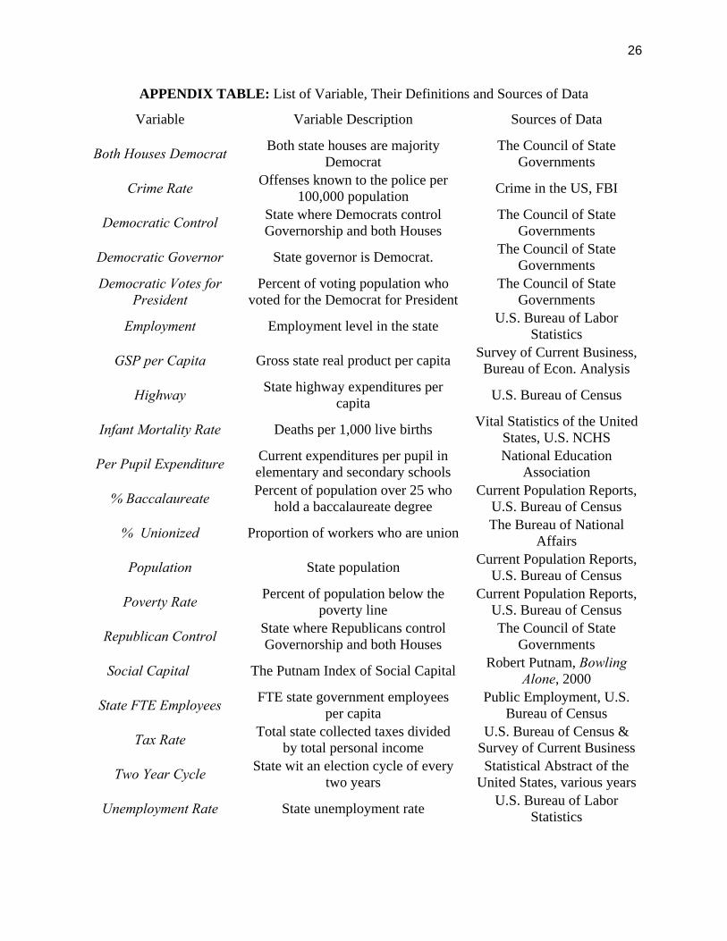
APPENDIX TABLE: List of Variable, Their Definitions and Sources of Data

Variable Variable Description Sources of Data

Both Houses Democrat Both state houses are majority Democrat

The Council of State Governments

Crime Rate Offenses known to the police per 100,000 population Crime in the US, FBI

Democratic Control State where Democrats control Governorship and both Houses

The Council of State Governments

Democratic Governor State governor is Democrat. The Council of State Governments

Democratic Votes for President

Percent of voting population who voted for the Democrat for President

The Council of State Governments

Employment Employment level in the state U.S. Bureau of Labor Statistics

GSP per Capita Gross state real product per capita Survey of Current Business, Bureau of Econ. Analysis

Highway State highway expenditures per capita U.S. Bureau of Census

Infant Mortality Rate Deaths per 1,000 live births Vital Statistics of the United States, U.S. NCHS

Per Pupil Expenditure Current expenditures per pupil in elementary and secondary schools

National Education Association

% Baccalaureate Percent of population over 25 who hold a baccalaureate degree

Current Population Reports, U.S. Bureau of Census

% Unionized Proportion of workers who are union The Bureau of National Affairs

Population State population Current Population Reports, U.S. Bureau of Census

Poverty Rate Percent of population below the poverty line

Current Population Reports, U.S. Bureau of Census

Republican Control State where Republicans control Governorship and both Houses

The Council of State Governments

Social Capital The Putnam Index of Social Capital Robert Putnam, Bowling Alone, 2000

State FTE Employees FTE state government employees per capita

Public Employment, U.S. Bureau of Census

Tax Rate Total state collected taxes divided by total personal income

U.S. Bureau of Census & Survey of Current Business

Two Year Cycle State wit an election cycle of every two years

Statistical Abstract of the United States, various years

Unemployment Rate State unemployment rate U.S. Bureau of Labor Statistics

27

Endnotes

1 Total government expenditures and spending on specific services. 2 See S. Pelzman's (1987) comments on this point (p. 293). 3 See discussion on this point in Adams-Kenny (1989) and also in S. Pelzman (1987) and Henrick and Garand (1991). 4 Helms (1985) has a detailed discussion on the effect of state government policies on the state economic growth. 5 Hendrick and Garand (1991) found that "...the state component of variance in state economic growth dominates the national and regional components during the post war era." p. 1101. 6 There are four states in which governors elect for only a two-year term. 7 During the act of voting, voters have the option to choose candidates for different elected positions by their party affiliation, i.e., party block. 8 Note that this 'naive' goal is consistent with the promise of candidates who are running for any office. Also note that this is not to say that everyone's gain is the same, or even to suggest that everyone gains something. The question about the distribution of gains may also depend on the political parties, but it is beyond the scope of this paper. 9 Hibbes (1987) also provides some empirical evidence on the difference between the two parties. "...the Democratic administrations typically turned in a real income growth rate that, ..., was about 1.2 points higher than the growth rates achieved by Republican administrations during the postwar period". (p. 268) 10 The regional rate of growth was calculated for each of the nine regions. For a more detailed discussion of this formula, see Nardinelli, Wallace and Warner (1988). 11 The number of states in which gubernatorial elections were held: in 1978-36 and two more in 1979, in 1982, 1986, and in 1990-36, in 1994, and in 1996. 12 No account was taken of the inflation rate at the individual state due to lack of data. 13 Gilligan and Matsusaka (1995) have been using a similar set political variables.