statewide climate projections summary€¦ · web viewin addition, heat can directly stress...

MASSACHUSETTS CLIMATE CHANGE PROJECTIONS

Researchers from the Northeast Climate Science Center at the University of Massachusetts Amherst developed downscaled projections for changes in temperature, precipitation, and sea level rise for the Commonwealth of Massachusetts. The Executive Office of Energy and Environmental Affairs has provided support for these projections to enable municipalities, industry, organizations, state government and others to utilize a standard, peer-reviewed set of climate change projections that show how the climate is likely to change in Massachusetts through the end of this century.

Temperature and Precipitation Projections

The temperature and precipitation climate change projections are based on simulations from the latest generation of climate models1 from the International Panel on Climate Change and scenarios of future greenhouse gas emissions.2 The models were carefully selected from a larger ensemble of climate models based on their ability to provide reliable climate information for the Northeast U.S., while maintaining diversity in future projections that capture some of the inherent uncertainty in modeling climate variables like precipitation. The medium (RCP 4.5) and high (RCP 8.5) emission scenarios were chosen for possible pathways of future greenhouse gas emissions. A moderate scenario of future greenhouse gas emissions assumes a peak around mid-century, which then declines rapidly over the second half of the century, while the highest scenario assumes the continuance of the current emissions trajectory.

Fourteen climate models have been run with 2 emission scenarios each, which lead to 28 projections. The values cited in the tables below are based on the 10-90th percentiles across the 28 projections, so they bracket the most likely scenarios. For simplicity, we use the terms “…expected to…,” and “…will be…,” but recognize that these are estimates based on model scenarios and are not predictive forecasts. The statewide projections comprising county- and basin-level information are derived by statistically downscaling the climate model results.3 They represent the best estimates that we can currently provide for a range of anticipated changes in greenhouse gases. Note that precipitation projections are generally more uncertain than temperature.

1These latest generation of climate models are included in the Coupled Model Intercomparison Project Phase 5 (CMIP5), which formed the basis of projections summarized in the IPCC Fifth Assessment Report (2013).2 Future greenhouse gas emissions scenarios are typically expressed as “Representative Concentration Pathways” (RCPs). They indicate emissions trajectories that would lead to certain levels of radiative forcing by 2100, relative to the pre-industrial state of the atmosphere; RCP4.5 equates to +4.5W m-2, and RCP 8.5 would be +8.5W m-2. In effect, they represent different pathways that society may or may not follow, to reduce emissions through climate change mitigation measures.3 The Local Constructed Analogs (LOCA) method (Pierce et al., 2014) was used for the statistical downscaling of the statewide projections.

1

The downscaled temperature and precipitation projections for the Commonwealth are provided at three geographic scales (Table 1) for annual and seasonal temporal scales (Table 2), and can be accessed through the Massachusetts Climate Change Clearinghouse website (www.massclimatechange.org). The statewide projections are included in this guidebook, but temperature and precipitation projections at each of the Commonwealth’s major basins are accessible on the website and as a supplemental PDF to this guide.

These climate projections are provided to help municipal officials, state agency staff, land managers, and others to identify future hazards related to, or exacerbated by changing climatic conditions. For the Municipal Vulnerability Preparedness (MVP) program participants, we recommend using climate projections downscaled to the major basin scale (Table 1) as there are regional differences across several climate indicators (Table 3). These projections can help MVP communities to think through how future hazards in their community may change, given projected changes in temperature and precipitation.

Regardless of geographic scale, rising temperatures, changing precipitation, and extreme weather will continue to affect the people and resources of the Commonwealth throughout the 21st century. A first step in becoming more climate-resilient is to identify the climate changes your community will be exposed to, the impacts and risks to critical assets, functions, vulnerable populations arising from these changes, the underlying sensitivities to these types of changes, and the background stressors that may exacerbate overall vulnerability.

Table 1: Geographic scales available for use for Massachusetts temperature and precipitation projectionsGeographic Scale DefinitionStatewide MassachusettsCounty Barnstable, Berkshire, Bristol, Dukes, Essex, Franklin, Hampden, Middlesex,

Nantucket, Norfolk, Plymouth, Suffolk, WorcesterMajor basins4 Blackstone, Boston Harbor, Buzzards Bay, Cape Cod, Charles, Chicopee,

Connecticut, Deerfield, Farmington, French, Housatonic, Hudson, Ipswich, Merrimack, Millers, Narragansett Bay & Mt. Hope Bay, Nashua, North Coastal, Parker, Quinebaug, Shawsheen, South Coastal, Sudbury-Assabet-Concord (SuAsCo), Taunton, Ten Mile, Westfield, and Islands (presented here as Martha’s Vineyard basin and Nantucket basin)

Table 2: Definition of seasons as applied to temporal scales used for temperature and precipitation projectionsSeason DefinitionWinter December-FebruarySpring March-MaySummer June-AugustFall September-November

4 Many municipalities fall within more than one basin, so it is advised to use the climate projections for the basin that contains the majority of the land area of the municipality.

2

http://www.massclimatechange.org/

Table 3: List and definitions of projected temperature indicatorsClimate Variable Climate Indicator Definition

Temperature

Average temperatureAverage annual or seasonal temperature expressed in degrees Fahrenheit (⁰F).

Maximum temperature Maximum annual or seasonal temperature expressed in degrees Fahrenheit (⁰F).

Minimum temperature Minimum annual or seasonal temperature expressed in degrees Fahrenheit (⁰F).

Days with Tmax > 90 ⁰F Number of days when daily maximum temperature exceeds 90⁰F.Days with Tmax > 95 ⁰F Number of days when daily maximum temperature exceeds 95⁰F.

Days with Tmax > 100 ⁰F Number of days when daily maximum temperature exceeds 100⁰F.Days with Tmin < 32 ⁰F Number of days when daily minimum temperature is below 32 ⁰F.Days with Tmin < 0 ⁰F Number of days when daily minimum temperature is below 0 ⁰F.

Heating degree-days(base 65 ⁰F)

Heating degree-days (HDD) are a measure of how much and for how long outside air temperature was lower than a specific base temperature. HDD are the difference between the average daily temperature and 65°F. For example, if the mean temperature is 30°F, we subtract the mean from 65 and the result is 30 heating degree-days for that day. HDD serves as a proxy that captures energy consumption required to heat buildings, and is used in utility planning and building design.5

Cooling degree-days(base 65 ⁰F)

Cooling degree days (CDD) are a measure of how much and for how long outside air temperature was higher than a specific base temperature. CDD are the difference between the average daily temperature and 65°F. For example, if the temperature mean is 90°F, we subtract 65 from the mean and the result is 25 cooling degree-days for that day. CDD serves as a proxy that captures energy consumption required to cool buildings, and is used in utility planning and building design. 6

Growing degree-days(base 50 ⁰F)

Growing degree days (GDD) are a measure of heat accumulation that can be correlated to express crop maturity (plant development). GDD is computed by subtracting a base temperature of 50°F from the average of the maximum and minimum temperatures for the day. Minimum temperatures less than 50°F are set to 50, and maximum temperatures greater than 86°F are set to 86. These substitutions indicate that no appreciable growth is detected with temperatures lower than 50° or greater than 86°.7

5 For seasonal or annual projections, HDD are summed for the period of interest. For example, for winter HDD, one would sum the HDD for December 1 through February 28. Degree-days are not the equivalent of calendar days and thus why it is possible to have more than 365 degree-days.6 For seasonal or annual projections, CDD are summed for the period of interest. For example, for summer CDD, one would sum the CDD for June 1 through August 31. Degree-days are not the equivalent of calendar days and thus why it is possible to have more than 365 degree-days.7 Definition adapted from National Weather Service. Degree-days are not the equivalent of calendar days and thus why it is possible to have more than 365 degree-days.

3

Table 4: List and definitions of projected precipitation indicators

Climate Variable Climate Indicator Definition

Precipitation

Total precipitation Total annual or seasonal precipitation expressed in inches.

Days with precipitation >1 inch Extreme precipitation events measured in days with precipitation eclipsing one inch.

Days with precipitation > 2 inch Extreme precipitation events measured in days with precipitation eclipsing two inches.

Days with precipitation > 4 inch Extreme precipitation events measured in days with precipitation eclipsing four inches.

Consecutive dry daysFor a given period, the largest number of consecutive days with precipitation less than 1 mm (0.039 inches).

Impacts from Increasing Temperatures

Warmer temperatures and extended heat waves could have very significant impacts on public health in our state, as well as the health of plants, animals and ecosystems like forests and wetlands. Rising temperatures will also affect important economic sectors like agriculture and tourism, and infrastructure like the electrical grid.

Annual air temperatures in the Northeast have been warming at an average rate of 0.5°F (nearly 0.26°C) per decade since 1970. Winter temperatures have been rising at a faster rate of 0.9°F8 per decade on average. Even what seems like a very small rise in average temperatures can cause major changes in other factors, such as the relative proportion of precipitation that falls as rain or snow.

In Massachusetts, temperatures are projected to increase significantly over the next century. Winter average temperatures are likely to increase more than those in summer, with major impacts on everything from winter recreation to increased pests and challenges to harvesting for the forestry industry.

Beyond this general warming trend, Massachusetts will experience an increasing number of days with extreme heat in the future (Table 3). Generally, extreme heat is considered to be over 90 degrees F, because at temperatures above that threshold, heat-related illnesses and mortality show a marked increase.

Extreme heat can be especially damaging in urban areas, where there is often a concentration of vulnerable populations, and where more impervious surfaces such as streets and parking lots

8 NOAA National Centers for Environmental information, Climate at a Glance: U.S. Time Series, Average Temperature, published December 2017, retrieved on December 21, 2017 from http://www.ncdc.noaa.gov/cag/

4

http://www.ncdc.noaa.gov/cag/

and less vegetation cause a “heat island” effect that makes them hotter compared to neighboring rural areas.

Urban residents in Massachusetts – especially those who are very young, ill, or elderly, and those who live in older buildings without air conditioning – will face greater risks of serious heat-related illnesses when extreme heat becomes more common. Extreme heat and dry conditions or drought could also be detrimental to crop production, harvest and livestock.

While warmer winters may reduce burdens on energy systems, more heat in the summer may put larger demands on aging systems, creating the potential for power outages. The number of cooling degree days is expected to increase significantly by the end of the century adding to this strain. In addition, heat can directly stress transmission lines, substations, train tracks, roads and bridges, and other critical infrastructure.

Impacts from Changing Precipitation Conditions

Rainfall is expected to increase in spring and winter months in particular in Massachusetts, with increasing consecutive dry days in summer and fall. More total rainfall can have an impact on the frequency of minor but disruptive flooding events, especially in areas where storm water infrastructure has not been adequately sized to accommodate higher levels. Increased total rainfall will also affect agriculture, forestry and natural ecosystems.

More intense downpours often lead to inland flooding as soils become saturated and stop absorbing more water, river flows rise, and the capacity of urban storm water systems is exceeded. Flooding may occur as a result of heavy rainfall, snowmelt, or coastal flooding associated with high wind and wave action, but precipitation is the strongest driver of flooding in Massachusetts. Winter flooding is also common in the state, particularly when the ground is frozen. The Commonwealth experienced 22 flood-related disaster declarations from 1954 to 2017 with many of these falling in winter or early spring, or during recent hurricanes.

The climate projections suggest that the frequency of high-intensity rainfall events will trend upward. Overall, it is anticipated that the severity of flood-inducing weather events and storms will increase, with events that produce sufficient precipitation to present a risk of flooding likely increasing. A single intense downpour can cause flooding and widespread damage to property and critical infrastructure. The coast will experience the greatest increase in high-intensity rainfall days, but some level of increase will occur in every area of Massachusetts.

Intense rainfall in urbanized areas can cause pollutants on roads and parking lots to get washed into nearby rivers and lakes, reducing habitat quality. As rainfall and snowfall patterns change, certain habitats and species that have specific physiological requirements may be affected.

5

Climate projections for Massachusetts indicate that in future decades, winter precipitation could increase, but by the end of the century most of this precipitation is likely to fall as rain instead of snow due to warmer winters. There are many human and environmental impacts that could result from this change including reduced snow cover for winter recreation and tourism, less spring snow melt to replenish aquifers, higher levels of winter runoff, and lower spring river flows for aquatic ecosystems.

A small projected decrease in average summer precipitation in Massachusetts could combine with higher temperatures to increase the frequency of episodic droughts, like the one experienced across the Commonwealth in the summer of 2016.

Droughts will create challenges for local water supply by reducing surface water storage and the recharge of groundwater supplies, including private wells. More frequent droughts could also exacerbate the impacts of flood events by damaging vegetation that could otherwise help mitigate flooding impacts. Droughts may also weaken tree root systems, making them more susceptible to toppling during high wind events.

6

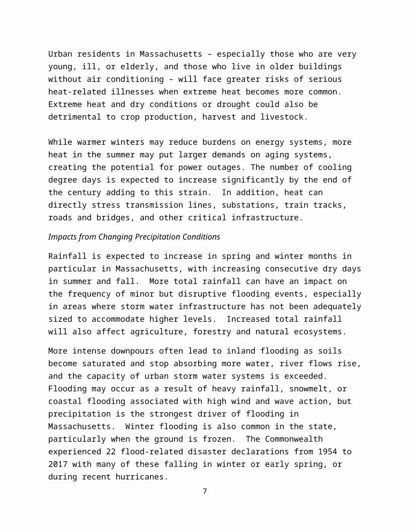
Table 5: Statewide projected changes of temperature and precipitation variables by the middle and end of the century, based on climate models and the medium and high pathways of future greenhouse gas emissions. Projected changes for each climate indicator are given as a 30-year mean relative to the 1971-2000 baseline, centered on the 2050s (2040-2069) and the 2090s (2080-2099).9 The values cited are the range of the most likely scenarios (10-90th percentile).

Climate Indicator

ObservedValue

1971-2000 Average

Mid-Century

Projected and Percent Change in 2050s (2040-2069)

End of Century


Average Temperature

Annual 47.6 °F Increase by 2.8 to 6.2 °FIncrease by 6 to 13 %

Increase by 3.8 to 10.8 °FIncrease by 8 to 23 %

Winter 26.6 °F Increase by 2.9 to 7.4 °FIncrease by 11 to 28 %


Spring 45.4 °F Increase by 2.5 to 5.5 °FIncrease by 6 to 12 %


Summer 67.9 °F Increase by 2.8 to 6.7 °FIncrease by 4 to 10 %


Fall 50 °F Increase by 3.6 to 6.6 °FIncrease by 7 to 13 %


Maximum Temperature

Annual 58.0 °F Increase by 2.6 to 6.1 °FIncrease by 4 to 11 %






Summer 78.9 °F Increase by 2.6 to 6.7 °FIncrease by 3 to 8 %


Fall 60.6 °F Increase by 3.4 to 6.8 °FIncrease by 6 to 11 %


Minimum Temperature

Annual 37.1 °F Increase 3.2 to 6.4 °FIncrease by 9 to 17 %

Increase by 4.1 to 10.9°FIncrease by 11 to 29 %





Summer 56.8 °F Increase by 3 to 6.9 °FIncrease by 5 to 12 %

Increase by 3.9 to 12 °FIncrease by 7 to 21 %

Fall 39.4 °F Increase by 3.5 to 6.5 °FIncrease by 9 to 16 %


9 A 20-yr mean is used for the 2090s because the climate models end at 2100.

7

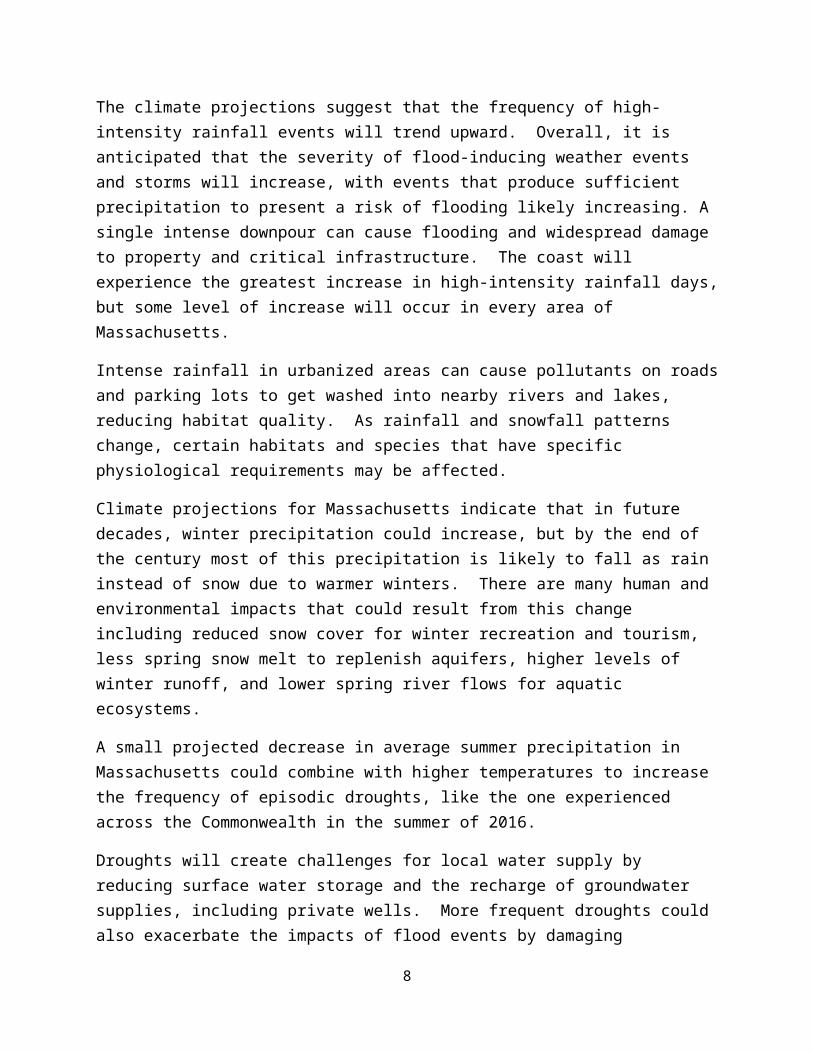
Table 5 Continued

Climate Indicator

Observed Value

1971-2000 Average

Mid-Century


End of Century


Days with Tmax > 90°F

Annual 5 days Increase by 7 to 26 days Increase by 11 to 64 daysWinter 0 days No change No changeSpring < 1 day10 Increase by 0 to 1 days Increase by 0 to 4 daysSummer 4 days Increase by 6 to 22 days Increase by 9 to 52 daysFall < 1 day9 Increase by 0 to 3 days Increase by 1 to 9 days


Annual < 1 day9 Increase by 2 to 11 days Increase by 3 to 35 days

Winter 0 days No change No change

Spring < 1 day9 No change Increase by 0 to 1 daysIncrease by

Summer < 1 day9 Increase by 2 to 10 days Increase by 3 to 32 days

Fall < 1 day9 Increase by 0 to 1 day Increase by 0 to 3 days


Annual < 1 day9 Increase by 0 to 3 days Increase by 0 to 13 days

Winter 0 days No change No change

Spring 0 days No change No change

Summer < 1 day9 Increase by 0 to 3 days Increase by 0 to 12 days

Fall 0 days No change Increase by 0 to 1 day

Days with Tmin < 32°F

Annual 146 days Decrease by 19 to 40 days Decrease by 24 to 64 days

Winter 82 days Decrease by 4 to 12 days Decrease by 6 to 25 days

Spring 37 days Decrease by 6 to 15 days Decrease by 9 to 20 days

Summer < 1 day9 No change No change

Fall 27 days Decrease by 8 to 13 days Decrease by 8 to 20 days

Days with Tmin < 0°F

Annual 8 days Decrease by 4 to 6 days Decrease by 4 to 7 days

Winter 8 days Decrease by 3 to 6 days Decrease by 4 to 6 days

Spring < 1 day9 No change No change

Summer 0 days No change No change

Fall < 1 day9 No change No change

10 Over the observed period, there were some years with at least 1 day with seasonal Tmax over (or Tmin under) a certain threshold while in all the other years that threshold wasn’t crossed seasonally at all.

8

Table 5 Continued

Climate Indicator

Observed Value

1971-2000 Average

Mid-Century


End of Century


Heating Degree-Days(Base 65°F)

Annual 6839degree-days

Decrease by 773 to 1627 degree-daysDecrease by 11 to 24 %


Winter 3475degree-days



Spring 1822degree-days


Decreases by 283 to 727 degree-daysDecrease by 16 to 40 %

Summer 134degree-days



Fall 1407degree-days



CoolingDegree-Days(Base 65°F)


Increase by 261 to 689 degree-daysIncrease by 57 to 151 %


Winter 0degree-days Increase by 0 to 5 degree-days Increase by 0 to 5 degree-days







Fall 40degree-days



Growing Degree-Days(Base 50°F)




Winter 5degree-days









Fall 429degree-days



9

Table 5 Continued

Climate Indicator

Observed Value

1971-2000 Average

Mid-Century


End of Century


Days with Precipitation

Over 1”

Annual 7 days Increase by 1 to 3 days Increase by 1 to 4 days

Winter 2 days Increase by 0 to 1 days Increase by 0 to 2 days

Spring 2 days Increase by 0 to 1 days Increase by 0 to 1 days

Summer 2 days Increase by 0 to 1 days Increase by 0 to 1 days

Fall 2 days Increase by 0 to 1 days Increase by 0 to 1 days


Over 2”

Annual 1 day Increase by 0 to 1 days Increase by 0 to 1 days

Winter < 1 day11 Increase by < 1 day10 Increase by < 1 day10

Spring < 1 day10 Increase by < 1 day10 Increase by < 1 day10

Summer < 1 day10 Increase by < 1 day10 Increase by < 1 day10

Fall < 1 day10 Increase by < 1 day10 Increase by < 1 day10


Over 4”

Annual < 1 day10 Increase by < 1 day10 Increase by < 1 day10

Winter 0 days No change Increase by < 1 day10

Spring 0 days Increase by < 1 day10 Increase by < 1 day10

Summer < 1 day10 Increase by < 1 day10 Increase by < 1 day10

Fall < 1 day10 Increase by < 1 day10 Increase by < 1 day10

Total Precipitation

Annual 47 inches Increase by 1 to 6 inchesIncrease by 2 to 13 %

Increase by 1.2 to 7.3 inchesIncrease by 3 to 16 %

Winter 11.2 inches Increase by 0.1 to 2.4 inchesIncrease by 1 to 21 %


Spring 12 inches Increase by 0.1 to 2 inchesIncrease by 1 to 17 %


Summer 11.5 inches Decrease by 0.4 to Increase by 2 inchesDecrease by 3 % to Increase by 17 %

Decrease by 1.5 to Increase by 1.9 inchesDecrease by 13% to Increase by 16 %

Fall 12.2 inches Decrease by 1.1 to Increase by 1.4 inchesDecrease by 9 to Increase by 12 %

Decrease by 1.7 to Increase by 1.4 inchesDecrease by 14 to Increase by 11 %

Consecutive Dry Days

Annual 17 days Increase by 0 to 2 days Increase by 0 to 3 daysWinter 11 days Decrease by 1 to Increase by 1 days Decrease by 1 to Increase by 2 daysSpring 11 days Decrease by 1 to Increase by 1 day Decrease by 1 to Increase by 1 daySummer 12 days Decrease by 1 to Increase by 2 days Decrease by 1 to Increase by 3 daysFall 12 days Increase by 0 to 3 days Increase by 0 to 3 days

11 Over the observed period, there were some years with at least 1 day with seasonal precipitation over a certain threshold while in all the other years that threshold wasn’t crossed seasonally at all.

10

Sea Level Rise Projections

Future sea-level projections are provided for the Massachusetts coastline at established tide gauge locations at Boston Harbor, Buzzards Bay, Nantucket, Newport, RI, Sandwich, Seavey Island, NH, and Woods Hole. The methodology for developing these projections closely follows the approach applied to Boston Harbor for Climate Ready Boston,12 and a recent analysis for the State of California.13 The analysis consists of a probabilistic assessment of future sea level at each tide gauge location and following two possible future greenhouse gas emissions scenarios: medium (RCP4.5) and high (RCP8.5).14 Relative Sea Level (RSL) is the local difference in elevation between the sea surface and land surface. A multi-year reference time period for RSL was used to minimize biases caused by tidal, seasonal, and interannual climate variability, following the common practice of using a 19-year tidal datum epoch15 centered on 2000 as the ‘zero’ reference for changes in RSL.16 Estimates of relative sea-level at site-specific locations and at individual years requires the consideration of processes not explicitly considered in the analysis.

Collectively, these sea level rise projections provide the background sea level estimates that can be used for detailed, site specific hydrodynamical modeling17 to map storm surge impacts, and influences of localized processes along the coast. For the MVP program, while not sight-specific or projections of mean higher high water levels, these projections provide insight into overall trends in rising sea levels along the Commonwealth coastline, to help coastal municipal officials and workshop participants identify future hazards exacerbated by rising seas.

Impacts from Rising Sea Levels

The impact of rising sea levels depends on local factors and geographies. The local impacts from sea level rise along our coast will be shaped by regional ocean currents, wind patterns, land and shoreland elevations, geomorphic processes such as subsidence and accretion rates (sinking and accumulation of sediment), and tidal zones.

12 Douglas, E., P. Kirshen, R. Hannigan, R. Herst, A. Palardy, R. DeConto, D. FitzGerald, C. Hay, Z. Hughes, A. Kemp, R. Kopp, B. Anderson, Z. Kuang, S. Ravela, J. Woodruff, M. Barlow, M. Collins, A. DeGaetano, C. A. Schlosser, A. Ganguly, E. Kodra, and M. Ruth (2016), Climate Change and Sea Level Rise Projections for Boston: the Boston Research Advisory Group Report, 54 pp. pp., Climate Ready Boston, Boston, MA.13 Griggs, G., Arvai, J., Cayan, D., DeConto, R., Fox, J., Fricker, H. A., Kopp, R. E., Tebaldi, C., Whiteman, E.A. and the California Ocean Protection Council Science Advisory Team Working Group (2017), Rising Seas in California: An Update on Sea-Level Rise Science. California, Ocean Science Trust, April 2017.14 Van Vuuren, D. P., Edmonds, J., Kainuma, M., Riahi, K., Thomson, A., Hibbard, K.,Lamarque, J.-F. (2011), The representative concentration pathways: an overview. Climatic Change, 109, 5-31.15 A tidal datum epoch is a 19-year period over which tidal height observations are taken and reduced to obtain mean values in order to establish the various datums (e.g., mean higher high water, etc.)(NOAA Tides and Currents).16 e.g., Sweet, W. V., R. E. Kopp, C. P. Weaver, J. Obeysekera, R. M. Horton, E. R. Thieler and C. Zervas (2017), Global and Regional Sea Level Rise Scenarios for the United States. NOAA Technical Report NOS CO-OPS 083.17 e.g., Bosma, K., E. Douglas, P. Kirshen, K. McArthur, S. Miller, S., and C. Watson (2015), Climate Change and Extreme Weather Vulnerability Assessments and Adaptation Options for the Central Artery. MassDOT, Boston MA.

11

For low elevation coastal areas, even a rise of less than a foot can produce significant new risks for development and infrastructure like the electrical grid and storm and waste water systems near the shore.

Sea level rise driven by climate change will exacerbate many other existing coastal hazards, like severe storms and storm surge, tidal inundation and salt water intrusion.

With rising sea levels, more regular flooding of developed and natural low-lying coastal areas is expected to occur due to more frequent tidal inundation. There will be increased erosion of existing coastal landforms (e.g., beaches and dunes). Damage to coastal engineering structures (e.g, seawalls) and more frequent flooding of coastal properties and neighrborhoods may occur as tidal range and wave energy increases.

As water levels rise, coastal storm surge events will cause inundation of larger areas, and will occur more frequently. Storm surges can damage or destroy coastal engineering structures, critical infrastructure such as waste water treatment plants or transportation systems, and private property. Massachusetts has highways, subway systems and rail lines located close to the coast.

Salt-water intrusion, or the increased penetration of salt-water into estuarine habitats, such as salt marshes and freshwater wetlands. It could alter the composition of the plant species and affect the wildlife that depend on these ecosystems. Water resources (such as drinking water) could also be impacted by salt-water intrusion and by the corrosion of important infrastructure.

12

Table 6: Sea level rise projections at the Boston tide gauge. Projections are given for the medium (RCP 4.5) and high (RCP 8.5) emissions scenarios, at multiple levels of likelihood, in feet relative to mean sea level in 2000.

Figure 1: Sea level rise projections at the Boston tide gauge. Projection curves are given for the medium (RCP 4.5) and high (RCP 8.5) emissions scenarios, at multiple levels of likelihood, in feet relative to mean sea level in 2000. These projections of sea level rise do not include potential contributions from significant losses of the Antarctic ice sheet.

13

Table 8: Sea level rise projections at the Nantucket tide gauge. Projections are given for the medium (RCP 4.5) and high (RCP 8.5) emissions scenarios, at multiple levels of likelihood, in feet relative to mean sea level in 2000.

Figure 2: Sea level rise projections at the Nantucket tide gauge. Projection curves are given for the medium (RCP 4.5) and high (RCP 8.5) emissions scenarios, at multiple levels of likelihood, in feet relative to mean sea level in 2000. These projections of sea level rise do not include potential contributions from significant losses of the Antarctic ice sheet.

14

Table 9: Sea level rise projections at the Woods Hole tide gauge. Projections are given for the medium (RCP 4.5) and high (RCP 8.5) emissions scenarios, at multiple levels of likelihood, in feet relative to mean sea level in 2000.

15

Figure 3: Sea level rise projections at the Woods Hole tide gauge. Projection curves are given for the medium (RCP 4.5) and high (RCP 8.5) emissions scenarios, at multiple levels of likelihood, in feet relative to mean sea level in 2000. These projections of sea level rise do not include potential contributions from significant losses of the Antarctic ice sheet.

Table 10: Sea level rise projections at the Buzzards Bay tide gauge. Projections are given for the medium (RCP 4.5) and high (RCP 8.5) emissions scenarios, at multiple levels of likelihood, in feet relative to mean sea level in 2000.

Table 11: Sea level rise projections at the Sandwich Marina tide gauge. Projections are given for the medium (RCP 4.5) and high (RCP 8.5) emissions scenarios, at multiple levels of likelihood, in feet relative to mean sea

16

level in 2000.

Table 12: Sea level rise projections at the Seavey Island, ME tide gauge. Projections are given for the medium (RCP 4.5) and high (RCP 8.5) emissions scenarios, at multiple levels of likelihood, in feet relative to mean sea level in 2000.

17

Table 13: Sea level rise projections at the Newport, RI tide gauge. Projections are given for the medium (RCP 4.5) and high (RCP 8.5) emissions scenarios, at multiple levels of likelihood, in feet relative to mean sea level in 2000.

18

statewide climate projections summary€¦ · web viewin addition, heat can directly stress...

Documents