Pacific Marine Science Report 77-12

STATIC ANALYSIS OF SINGLE-POINT MOORINGS

by

W.H. Bell

Institute of Ocean Sciences, Patricia Bay

Victoria, B.C.

August 1977

This is a manuscript which has received only limited

circulation. On citing this report in a bibliography,

the title should be followed by the words "UNPUBLISHED

MANUSCRIPT" which is in accordance with acceJ?ted bib­

liographic custom.

i

ABSTRACT

A static mooring model is developed for use in the design and analysis of moored instrument arrays. The model incorporates the steady two­dimensional hydrodynamic forces exerted by a space-varying velocity field on a surface or subsurface buoy and on a flexible, extensible cable and instruments supported beneath the buoy. Suitable equations for the normal and longitudinal components of cable drag are provided from an examination of existing data. The model behaviour is verified using an analytical solution for a free-streaming cable. An example is given of the model applied to a mooring which consists of a toroidal surface float, an extensible synthetic plastic cable, five instrument packages and a heavy chain anchor.

ii

TABLE OF CONTENTS

Abstract-

Table of Contents

List of Figures

Li st of Tables

Introduction

Theoretical Analysis of a Buoy-Cable System

A. The Buoy

B. The Cable

C. Cable Drag

D. The Instruments

E. Method of Solution

Computer Solution of The Buoy-Cable System

A. The Buoy

B. The Velocity Profile

c. The Instruments

D. The Cable

E. The Iteration Procedure

F. Program Output

Verification of the Model

Limitations of the Present Model

References

Appendix A - Buoy Calculations

Appendix B - Sample Computation

Appendix C - Program Source Listing

Page

- i

ii

ii;

iii

1

2

2

3

8

16

18

18

18

18

19

19

21

22

22

24

25

26

28

38

iii

LIST OF FIGURES

Fig. Buoy Free-body Diagram

Fig. 2 Cable Free-body Diagram

Fi g. 3 Drag of Smooth Cylinders

Fig. 4 Normal Drag Coefficient .~ Cable Inclination

Fig. 5 Longitudinal Drag Coefficient ~ Cable Inclination

Fig. 6 Drag Force Component Magnitudes

Fig. 7 Instrument Package Free-body Diagram

LIST OF TABLES

Table I FORTRAN Coding Form for Mooring Program Example

Table II Output Listing for Mooring Program Example

Page

4

6

11

12

14

15

17

31

32

1

Introduction

The Coastal Zone Oceanography Group at the Institute of Ocean Sciences, Patricia Bay, makes widespread use of moored instrument arrays for the measurement of seawater properties. The moorings are usually single-point taut-l ine types, supported by either a surface or a subsurface buoy~ with a length ,of heavy chain or a clump of railway wheels and a Danforth anchor at· the lower end. The moorings are normally made in fairly protected waters, so the response to wave action is not often a problem. However, questions have arisen from time to time concerning the actual depths of the instruments. For subsurface buoys, drag forces on the whole system can result in a considerable. reduction in the elevation above bottom of any point in the system. For surf~ce buoys, where synthetic lines are normally used, the stretch of the line can cause uncertainties in instrument positions. The elevations could be determined, after the fact, by using depth. sensors, but it was desirable to have some· means of estimating the instrument positions, for a glven set of conditions, before deploying an array. Thus a theoretical investigation of the static behaviour of taut-line moorings was indicated.

A survey. of available literature (e.g. McCormick, 1973; Schram, 1968) indicated there were some existing mooring models, most of them not as comprehensive as one might desire, and none of them completely suitable for our needs. Therefore, we decided to develop a mooring system model specifically oriented to the requirements Of the group. It would incorporate such:.details as, a varying velocity profile, elastic cable, varying cable types, surface or subsurface buoy, attached instruments and slack or taut line intopne computer program. A two-dimensional model was deemed sufficient for our purposes: The informat'ion avail abl e from such a model incl udes:

the "length to which an elastic line should be cut for a taut-line surface mooring in a given water depth;

- the attachment points along the unstretched cable for instruments to end up at the required depths;

- the differences in a taut-line surface mooring configuration fof low and high tide situations;

- the required buoyancy to attain or maintain a particular depth with a subsurface buoy;

- the tension in the mooring line; - the required minimum anchor weight; - the horizontal excursion of the mooring; - the excursions through depth of instruments suspended below a

subsurface buoy for various velocity profiles; the line angle at any point along its length.

The mooring model development is outlined in the following sections. The engineering system of units (ft-lb-sec) is used throughout the model, in preference to the metric system, because of the present utility of the engineering force unit in connection with the purchase and use of cables, buoys and anchors.

2

Theoretical Analysis of a Buoy-Cable System

A. TheSuoy

Several types of buoys, having various shapes, are used ln moorings. The toroidal buoy has been the most commonly 'used type for sur,face floats. It supports. a tripod superstructure for increased visi'bility. The small amount of wind drag on the superstructure, and on the exposed portion of the buoy, will be ignored here, as will the effect.of buoy tilt due to waves. Sub­surface moorings are usually effected with spherical buoys, or with cylindri­cal buoys having a horizontal axis. The l~tter include tail fins to provide stability. If such a buoy' develops a large degree of tilt, then an analysis of the .forces involved can become very complicated. For example, the . separate lift and drag forces of the 'main body and the fins, together with their moments about the centre of gravity (CG), must be considered. 'The lift and drag coefficients,'and their points of action, will be functions of the'angle of tilt. The'buoyancy', weight and tensile forces will be unlikely to act through' the same point, creating additional moments to complicate the problem. For such a case, the obvious solution is to redesign the buoy' fOf ad~quate longitudinal stability at small tilt angles~ Principally, this requires tail fins of sufficient size to respond to small disturbance~~ suitci~ly.placed to avoid a loss of efficiency if sepa~at~6nof flow occurs oVer any portion of the buoy. Surface or subsurface buoys which aresymmei'rical about a vertjcal axis present no problems' due to' tilt, provided that the,l ift and drag coefficients do not change by any substantial ~mount over the r~n~e of tilt angles. There will be moments involved if the tehsil~ force in'tbec~bJ~ doesn't act along the axis (unless the' cable is . attached at the CG position), and if the centre o'f buoyancy (CB) doesn't . correspond approximate'ly with the eG. The simplest case will be considered here, the basic assumptions,being:.

1 . The line of actlon of the cable tension is through the CG of the buoy.

2. The point of cable attachment is at the lower surface of the buoy.

3. There is no change in drag coefficient with a change in buoy aspect.

4. There is no fluid dynamic lift force.

5. There is no wind drag.

6. The water drag is proportional to the greatest immersed cross­sectional area in a vertical plane normal to the flow direction.

7. There is no buoy tilt insofar as buoyancy and drag calculations are concern.ed.

The justification for the simplifications made in these assumptions is that the buoy drag will seldom be as important as cable drag in determining the system configuration, and that small tilt angles will not much affect the

3

buoyant force. Appendix A contains the immersed area and volume calculations for several buoy types.

A free-body diagram of a simple buoy is shown in Figure 1. ·A summation of forces in static equilibrium gives:

(1)

(2)

Here, B is the buoyancy force, obta·ined from the immersed volume. weight force, TB is the cable tension and ~B is the cable angle. force, 0, is represented by:

W is the The drag

o = Co 12- AVIVI (3 )

where Co is the drag coefficient for the shape under consideration, p is the flui.d density, A is the immersed area (Appendix A) and V is the fluid velocity. Solving equations (1) and (2) simultaneously, one obtains:

(4)

(5)

TB and ~B form the boundary conditions at the upper end of the cable.

B. The Cable

Cables used for mooring are of two principal types - synthetic (plastic) rope and wire rope. Occasionally, a section of chain may be included. Cables are probably the most difficult part of the system to analyze accurately since some of their characteristics are ill-defined. Further paragraphs of this section will examine the problem in more detail. For the present, it is sufficient to assume the following:

1. The cable is flexible and extensible.

2. The cable diameter is not significantly reduced when stretching occurs, i.e., the radial strain is neglected for the purpose of calculating the drag cross-sectional area.

3. The drag on the cable can be separated into normal and

4

B

v

Ts

BUOY FREE -BODY DIAGRAM

Figure 1

5

longitudinal components.

4. There are no side forces on the cable and no vortices are shed in the wake (thus, there is no possibility of "strumming").

5. The cable lies in a vertical plane and the flow is coplanar with the cable.

A free-body diagram of a cable segment is shown in Figure 2. The unstretched case is illustrated for simplicity. The independent variable is taken to be the length S along the cable. The dependent variables are then the cable angle ~ and tension T, and the x and z coordinates for any point on the cable. An elemental length of the cable is represented by bS. The weight force and buoyant force of the cable are, respectively, wand b pounds per unit length. The drag force DC is also in pounds per unit length and is shown resolved into normal and longitudinal components, FN and FL, respectively. The appropriate form for these components, especially FL, is open to some conjecture and will ·be considered in detail in the next section.

Resolving all of the forces into components, and summing in the normal and longitudinal 9irections, respectively, one obtains:

2T sin b: = {FN + (w-b) cos ~}bS

bT cos ~ = {- FL + (w-b) sin ~}bS

(6)

(7)

Taking these equations to the infinitesimal limit, and neglecting second order quantities, gives:

~~ = i {FN + (w-b) cos ~} (8)

dT _ dS - -FL + (w-b) sin ~ (9)

In addition, there are two parametric equations (directional derivatives) describing the cable shape, namely:

dx _ dS - cos ~ (10)

dz _ CiS - sin ~ (11 )

The preceding four equations are all that are necessary to describe an inextensible cable. They can be solved simultaneously, obtaining the boundary conditions from the buoy equations and from a condition on the water

. VI-

/ /

~

/ /

/

6

/ /

/

T ·~T +-2

;'

/ /

CABLE FREE-BODY DIAGRAM

Figure 2

7

depth, to provide the configuration of the cable and the tension in the cable. However, if the cable is extensible, with an elongation per unit length represented by £, an additional relationship is required to relate this strain to the tension in the cable. For materials obeying Hooke's law:

(12 )

where E is the static modulus of elasticity, A is the load-bearing cross­sectional area, L is theunstretched length of cable and 6L is the actual elongation. The strain of non-Hookeian (non-linear) materials is best approximated by fitting a power curve to empirical data, if such is available. The information regarding elongation of a particular material is often provided by the manufacturer in the form of a graph or table giving strain vs. the ratio of cable tension T tO,ultimate strength Tmax , both in percen­tages. In this case, one can obtain the strain in the form:

[,2-]+ 100 c max

(13)

where a, b, c are constants to be determined from the graph. Only the portion of the gr~ph covering the normal working range of the material should be consider~d. The cohsidefations above assume that pre-stretched cable is used, so that any elongation resulting from mechanical deformation (readjustment of strarid positioris)is nbt included.

Synthetic plastic cables are non-linear in their elastic behaviour, but the situation is complicated further by their plastic behaviour. This is especially so when a history factor is involved, that is, the stress-strain relationship depends somewhat on the previous loads experienced by the cable, and may be affected by the number of wet/dry cycles undergone. Also, some materials creep unde~ load, even after pre-stretching has settled the strands along the core. Some materials (e.g., nylon) absorb water and swell .. This can result in a contraction of cable length, because the expansion in the plane of the cross-section forces individual strands into a longer helical path about the core. Little of an exact nature is known about these effects and they are not dealt with here since their influence on the static behaviour of the mooring is normally small.

The total strained length of cable is (1 + £) times the original unstretched length. From Equation 13, we obtain the form used in the present model:

(14 )

where ao, aI' a2 are constants to be determined, as before. For an inextensible cable: aQ = 1, al = 0, a2 = O. For a cable obeying Hooke's Law: ao = 1, al = 4/(~d2 E), a2 = 0, where E is Young's modulus for the cable itself (not the modulus for the cable material because of the difficulty in

8

determining the exact cross-section area). 2For synthetic c~b1es: . ao = 1 + (aIlOO), al = b/Tmax , a2 = 100 c/Tmax , where Tmax lS the u1tlmate. stress for the cable. Rewriting equations 8 through 11 in terms of a strained element gives:

dx - (1+8) cos ,j, dS - 'I'

dz _ ( ) dS - 1 +c si n </>

( 15)

(16 )

( 17)

(18 )

Here, the implication is that the weight of one foot of stretched cable is w/(l+E) so there is no change in total weight. Further, the buoyancy per foot of stretched cable happens also to be taken as b/(l+E), so that some compensation for the. effect of radial strain on the displaced water.volume is included, although not in the correct formal manner .. Any error in 'this term ;-5 small compared to the other forces i nvol ved, so it was not consi dered necessary to formalize it. As mentioned previously, the effect of radial strain on the drag force term is neglected~ again because of its relative insignificance.

C. Cable Drag

A suitable representation ®f the cable drag forces is a very important consideration·for any mooring model, the more so when high,current speeds are involved since the drag is proportional to the square of the velocity. For the most part, the literature is not too helpful in this matter.· Usually, as is done here, the forces involved are resolved into components normal to the cable axis and components along.the cable. The form of the normal component of drag is almost standardized, although there is a considerable range in the actual drag coefficient values used. Many different forms have been proposed for the longitudinal component (Casarel1a & Parsons, 1970), but it is often ignored completely since it is usually small compared to the normal component. However, this is not necessarily the case when the cable angle becomes large for some reason, such as high water velocities or inadequate buoyancy on a subsurface mooring. Relative magnitudes will be examined below. A problem that confronts one in attempting to determine the most suitable form for drag force components is that very few measurements of force as a function of cable inclination to the flow have been reported'and some of these do not appear to be reliable, especially where longitudinal drag is concerned. This latter quantity is a difficult one to measure accurately because of its relative magnitude and the fact that

9

it is usually the result of the subtraction of two large quantities, the drag of the supporting structure being included in the measurement. The preferred data set, in my view, is that due to Relf and Powell, made in 19l7! Their longitudinal drag curve for a smooth wire is a good fit to a theoretically-derived form, as will be shown, with the lack of scatter in the data points being an indication of reasonable accuracy in the measure­ments. This gives one some confidence in their subsequent drag determinations for wire ropes. The Relf and Powell data is used below to estimate normal and longitudinal drag coefficients for cables inclined to the flow.

According to the "crossflow" or lIindependence ll principle which states, in effect, that the nature of the boundary layer depends only on the normal velocity component (Hoerner, 1958; Schlichting, 1960), the pressure force and the normal friction force will also depend only on that component. This holds true while laminar (sub-critical) flow prevails but does not necessarily apply to turbulent boundary layers. Thus, in sub~critical Reynolds number flow, the total drag force normal to the cable axis can be expressed as a function of V sin ~, where V is the free-stream velocity and ~ is the cable inclination referenced to a horizontal plane (Fig. 2). Typical mooring systems will almost always operate in the sub-critical flow regime. We can define the normal drag force component,per unit length of cable, as:

(19 )

where u = V sin ~ and d is the cable diameter. CDN is based on frontal area and includes the effects of both pressure and skin friction, i.e.

( 20)

Over the Reynolds number range of interest, say 102<R<105, Cp is usually considered approximately constant. It is much larger than CFN except at the low end of the range. The logical definition for Reynolds number here makes use of the normal velocity component as the characteristic velocity, since it is the key to the changing state of the boundary layer, as suggested by the independence prin~iple. Thus,

RU = dV ~in ~. = R sin ~ (21)

where v is the kinematic viscosity and R is the Reynolds number at ~ = 900•

Since it 1S R which is generally reported in the literature, its use in various~expressions w11l be retained here, but in conjunction with sin ~. The valu~ of Ru may become small at large cable angles, even though the free stream velocity is high, with the result that the friction component of the normal drag force may assume some relative importance. Therefore, CFN should probably not be excluded from consideration.

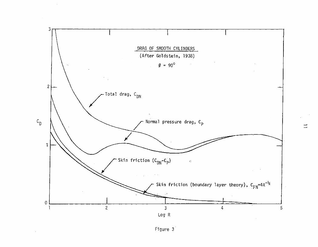
10

Goldstein (1938) presents some drag data, which he attributes to Relf arid Thorn, for a smooth cylinder normal to the flow. This is shown in Fig. 3. The total drag curve is by Relf; the rest of the results are due to Thorn, who derived a numerical solution for skin friction and found that a good fit to the points provided by this solution was given by:

4 - -1

R ~ u

(22)

for ~ = 90°. With the inclusion of the Reynolds number in the appropriate form, the effect of cable angle is accounted for, i.e.

CFN = __ 4...:----:-_ 1

(R sin ~)~ ( 23)

This equation should hold so long as the flow is laminar, at least. Thus, it may not apply to rough cylinders such as wire rope. An examination of the pressure drag curve in Fig. 3 suggests that, rather than taking it as constant, a power law fit might be worthwhile. In any case, the normal force has the form:

(24)

where Cp is determined at the angle ~ = 90° and R = dV. . v

. The p'reviously mentioned Relf and, Powell (R&P) data were obtained using a smooth wire and several different wire ropes. The data were taken near R = 104 , so that the friction drag is only a small fraction of the pressure drag. Even at an extreme angle of ~ = 100 , the boundary layer Reynolds number Ru is about 10 3 • Then the friction drag is about 1/10 of the pressure drag, so it is probably hidden within the measurement error of the small forces involved. The normal drag coefficient values, derived from R&P normal force measurements, are plotted in Fig. 4. The measurements on the different cable types were made at slightly different values of R, but the scatter in the data is more likely due to differences in cable construc­tion rather than to any R-dependence. The solid line in the figure is a sin2~ curve, which is readily fitted to any of the data sets, including both the smooth wire and the wire ropes.

The longitudinal, or along-cable, flow field is, in one sense, influenced by both flow components. This is a result of the fact that the

CD

3rr.-------------------~r----------------------r----------------------r---------------------~

1

DRAG OF SMOOTH CYLINDERS (After Goldstein, 1938)

o = 90°

~Total drag, CDN

pressure drag, Cp

Skin friction (boundary layer theory.), CFN=4R-~

I ~ o . I. 2 3

Log R

Figure 3

4 5

--' --'

z 0

()

1.4jr-------.--------r-------,--------r-------.r-------.--------.-------.------~

1.2

I.d- 0

• X D

0.8~

0.6~

0.4

CABLE TYPE

SMOOTH WIR~

BRITISH CABLE, 6X24

BRITISH CABLE, '6X37 GERMAN CABLE,7X7

NORMAL DRAG COEFFICIENT VS., ....

CABL,E·· IN'CLlNATION

DIAMETER (IN.) R

3/8 7,850 1-1/4 8,100

1-1/2 10,630 1-3/8 9,3.70 .

(DATA FROM RELF e. POWELL ,1917)

8

0./ ,( ;N2 CP

o

D ~. • I X

X X

0.2

% -~ ~ ~ k ~ ~ k ~ ~

Figure'4

..... N

13

boundary layer thickness is determined by the normal velocity component. A boundary layer build-up in the direction of the cable is prevented because the normal velocity "blows" away any excess retarded fluid layer. (This theory obviously breaks down for the limiting case of pure longitudinal flow at ~ = 00.) However, the longitudinal stress distribution within the boundary layer is determined only by the along-cable velocity., ,~Jhen the stress distribution is known it can be integrated over the cable to obtain the longitudinal drag force. The method for making this calculation has been suggested by Schlichting (1960) and carried out by Schram (1968) ~nd Topham (1976) for the case of a smooth cylinder. A similar solution to the problem is arrived 'at through an analogy with the heat flow equation (Schlichting, 1960; Taylor, 1952). The theoretical result is a function which depends on both the sine and cosine of the angle ~ (and not simply on COS2~ in an analogous fashion to the normal drag force), namely:

(25 )

where CL is a constant to be determined and GFL is based on surface area. There is no longitudinal pressure drag component because it is assumed that the cable' is infinitely long'. Note that, for convenfence in subsequent manipulation, we may write:

C - CL ( 16 ] ~. (26) FL - 4 R sin ~J cos, ~ S1n ~

The longitudinal drag criefficients derived from R&P data are shown in Fig. 5. The empirical result for the smooth wire shows good agreement with Equation 25. However, the wire rope data shows considerable variance from this function. This is probably a consequence of flow modification resulting from the spiral construction of the cable. Fitting a straight line to the wire rope data gives a curve of the form:

GFL - 1 - 90 R sin ~ -[ ~J [ 16 J ~ sin ~ (27)

where ~ is in degrees. All of the data were obtained near R = 104 , as previously mentioned. If this is beyond the flow transition point for the rough cab'les involve'd, then the boundary layer theory is inapplicable in any case. The relatively high normal drag coefficients (seen in Fig. 4) would seem to argue, though, that the flow is still sub-critical. Just where the transition region lies for such cable has not been determined, to my knowledge.

Fig. 6 summarizes the foregoing equations and allows one to easily determine the relative magnitudes of the component forces at a given cable inclination and Reynolds number. It can be seen that there may be occasions

4.0~K------~------~------r------'------~-------r------'-------~----~

3.0

I~~ . ~2.0 -l u..

C,.)

1.0

x 8

•

iI

o

LONGITUDINAL DRAG COEFFICIENT VS

8.

x.

CABLE INCLINATION

CABLE TYPE

o SMOOTH WIRE • BRITISH. CABLE, 6X24

X BRITISH CABLE, 6X37 8 GERMAN CABLE,7X7

DIAMETER (IN.)

3/8 1-1/4 1-1/2 1-3/8

(DATA FROM RELF a POWELL ,1917)

• / ""8 40-cf>

90 • 8. X

8

R

7,850 ~,IOO

10,630 9,370

o b io 210 3~ 40 50 ~O 7'0 . ~o . ""90

Figure 5

...... ~

"

100

I.L. .:.::

50

20.

10

5

2

k= I

DRAG FORCE COMPONENT MAGNITUDES

0/ 'Z. 4> \/'2. 5\t\

\ .'2.?-

L1L

R=I04

f dy2 v'Sincp td"",\/4" , V""'\ His)

::: 477"0_ -+=-t/90) ~ ~ kF ~

v_____ X

-------1-(8) ::: 18 ~ -- . 77"C 'I<...... ----... -..?S¢ _-=:::-...--e-----e----.-:>-__ -e-- ..........

...h _(!) .'.. "-

/Jr5\t\'1' ___ - "-. "" ~ -6- -, C": .. \~ ~5~ ...--~ -". ~~~- , /~ ~ '" .

F NP - NORMAL PRESSURE FORCE '-'--'_ "'-

FNF - NORMAL SKIN FRICTION -'--,_ ~ FL - LONGITUDINAL SKIN FRICTION \. \

S - ~OWH \

R - ROUGH \\ \

5 (DEGREES)

Figure 6

f

90

--' (J'1

16

on which the skin frictional forces should not be ignored. However, the equations are derived or verified on the basis of very limited empirical results. A definite need exists for force measurements on various cable types inclined to the flow over a reasonable range of Reynolds numbers. For the present, however, we will be satisfied to use the results outlined in Equations 19 through 27 to simulate drag in our mooring model.

D. The rnstruments

rnstrument packages, attached to the cable, may be of various shapes and sizes, and the method and points of attachment may vary. Here, as for the buoy, only the simplest case is considered, namely one in which all of the forces act through the CG and any effect of tilt is neglected. A free-body diagram is presented in Fig. 7. Wr is the package weight in air, Br is its buoyancy,. ~~ is the increment in cable angle due to the instrument and~T is the increment in cable tension. Package drag is given by:

( 28)

w~ere Cr is the~r~g coeffi~tent and A is the cross-sectional area presented to the flow. Reso~ving the forces in directions parallel to and normal to the cable and summing, one obtains, respectively:

,.

T+~Dr cos ~ - ~Wr-Br) sin ~ = (T-~T) cos ~~ (29)

(30)

Some of the instrument packages may be very buoyant or very heavy, so the simplifying assumption of small changes in angle cannot be made. Solving the equations simultaneously:

Dr sin ~ + (Wr-Br) cos ~ T - ~ T = ______ ---==---__ sin ~~

~~ = tan- 1 [Dr sin ~ + (Wr-Br) cos ~ 1 T + Dr cos ~ - (Wr-Br) sin ~

(31 )

( 32)

The boundary conditions (tension and angle) for these equations are obtained from the solution of the cable system on one side of the instrument. The equations, in turn, provide the boundary conditions for the next cable segment.

v

17

BI

----------- -

> I

~\/

/ I

I I L--..-+-~

WI

01

INSTRUMENT PACKAGE FREE -BODY DIAGRAM

Figure 7

18

E. Method of Solution

The equations for the complete buoy-cable system are first-order non-linear and form a boundary-value problem requiring boundary conditions at each end of the cable. The buoy boundary condition is satisfied by assuming an elevation for the buoy which, in turn, fixes the cross-sectional area and volume immersed. The anchor boundary condition is that the elevation of the anchor must coincide with that of the sea bottom, within acceptable limits. The governing equations are solved for the unknown quantities (~, T, x, z) by a step-wise integration along the cable, beginning at the buoy end, to a point df discontinuity resulting from the concentrated loads cqused by the presence of an instrument package. The effect of the forces o~ the package is added to the cable forces and the integration is continu~d-in a similar fashion until the lower end of the cable is reached. If the anchor boundary condition is not satisfied within the specified error limits"th,en a new buoy position is chosen and the procedure is repeated.

Computer Solution of the Buoy-Cable'System

A. The Buoy

The b~o¥ geometr:y is incorpo.rat~d ..into a subroutine (Appendix C), so that the abi 1 ity to cope with vari ous types of buoys"can be a'dded to the program with no difficulty.' The subroutine,'is,' entered with the buoy elevation and the water velocity at that elevation. The buoyancy and water drag forces are calculated and returned to the main program to provide the upper boundary condition on the cable. The limitatiQns' on these calculations have been mentioned in a previous section. The buoy elevation is taken to be at the bottom of the buoy, which is the point of attachment for the cable. Thus, for a surface buoy, the difference between the water'surface el evation and the buoy elevation is the depth of immersion of the buoy •. Three pertinent dimensions of a buoy can be spetified in the data input; The vertical dimension of the buoy is of particular importance, since,it is used in conjunction with the buoyancy to modify the position of the 'buoy during the iteration procedure. Surface or subsurface buoy types are specified by a flag in the main program, to permit some minor processing differences.

B. The Vel bdty Profil ~

Since the model is two-dimensional, the water motion is confined to a vertical plane. The flow is also assumed to have no vertical component. Any speed versus depth relationship which can be represented by a second order profile of the form:

v = a + bz + cz2 (33)

19

is permissible. Likewise, various profiles of this form can be pieced together in segments, as desired. The profile segments can be any convenient size and do not have to correspond to multiples of the cable segment length (discussed in a following section). Negative speeds are allowed. The only limitation is that strong discontinuities in the profile may make convergence to the correct solution more difficult. In the program, the velocity profile information is stored in an array, the first element in each row being the lower depth limit of applicability (measured from the sea-bed) of the particular segment whose coefficients (a,b,c) are given by the other elements of that row. Presently, storage is provided for five segments. A conditional branch on the depth is used in subsequent calculations to calculate the correct velocity for'a given depth.

C. The Instruments

The program permits all kinds of instrument packages to be inserted in the system. They should be positioned at multiples of the basic cable segment length, as used for integration along the cable (and discussed in the next section). If they are not so positioned, the program will round the position to a segment multiple. The instrument locations, in feet along the cable from the buoy, are read into the computer, converted into an integer number of cable segments and stored in an array capable of holding ten different values. Because of the conversion, the instrument locations are still correct when the cable is stretched. Before each integration is made 3 the program checks to see if there is an instrument at the upper end of the cable segment. If so, the velocity is determined and the instrument drag calculated. Then the resulting increments in cable tension and angle are combined with the preceding values of these variables. No separate subroutine is provided for the instruments, as was the case for the buoy, so the buoyancy and drag cross-sectional area must be read in as data. Any swivels, shackles or other fittings located near an instrument should have their weights accounted for by including them in the instrument weight.

D. The Cable

The integration along the cable is carried out over a series of cable segments which are of equal length when unstretched, this length being a sub-multiple of the total cable length. The choice of segment size depends on the problem parameters, such as the complexity of the velocity profile, the number and location of instrument packages, etc. The integration routine uses the Runge-Kutta method with error control. The user must code an external subroutine which specifies the functions required for an evaluation of the derivatives given in Equations 24 through 27. The integration routine also requires the specification of an error tolerance on the integral, a step size, and a value of the independent variable at the end-point of the integration. Double precision is used throughout to reduce the possibility of cumulative rounding errors.

For an extensible cable and step-wise integration, the end point

20

must correspond to the strained length of each cable segment. This requires that the independent variable be stretched as well, i.e. Equations 24 through 27 are divided through by the quantity (1 + E), giving (1 + E)dS as the independent variable instead of dS. In the program, the strained unit length (1 + E) is represented by the function STRCH. The function is presently calculated on the basis of the tension at the upper end of a cable segment~ For greater accuracy, this tension could include one-half of the tension increment for the previous segment. Generally speaking, however, the increment is usually no more than a few tenths of one percent of the tension, so this correction is ignored here. If required, the accuracy can be improved by reducing the segment length. Any necessity for this is easily checked by running the model for two different segment lengths.

The boundary conditions for the first cable segment are provided by the buoy calculations, and for subsequent segments by the results of the integration over the preceding cable segment. The velocity used for calculating cable drag is that which occurs at the midpoint of the segment, the midpoint elevation being estimated on the basis of the cable angle for the preceding segment. An iteration on the cable angle would result in a slightly more ~ccurate midpoint location and, therefore, a slightly more accurate velocity (only when the ve" ocity profil e is not uniform). Thi s was not deemed worthwhile since, for the calculation of drag, the midpoint velocity is assumed to apply over the whole segment in any case. Likewise, one could incorporate a varying velocity (when such is the case) throughout the integration over a cable segment, but at the expense of a considerable increase in program complexity. Again, if concern is felt about the outcome of the procedure as presently used, especially when the velocity is changing rapi dly with depth. the program can be run wi th sma 11 segment 1 engths. Some trial runs in which the segment lengths were varied by factors of two or more, all other variables remaining unchanged, showed no variation in the results. Thus, the indiGation is that the simple procedure used to obtain the velocity for the drag determination is adequate. Also, while only an average velocity value ;s used in the drag calculation, the dependence of the drag on the actual cable angle is included throughout th~ integratiori along a cable segment since the angle is one of the. dependent variables. At the conclusion of each call to the integration subroutine, the resulting cable angle is tested for a negative value. The program is terminated if such a value occurs, since it indicates either that the buoy has insufficient buoyancy or that the cable is much too long. Thus the model will only cope with a slack line mooring up to the point at which the slack is sufficient to result in a portion of the cable assuming a horizontal position. The length of cable involved, at this critical point, depends on the cable loading.

The mooring line used in the model is not restricted to one size or one kind of material throughout its length. Presently, ten different cable types can be handled. Information on these, including the lower end position of each type in feet from the buoy, is read into an array. Then (as is done for the instruments), the end position is converted into an integer number of cable segments, the conversion permitting an easy check on type changes as well as allowing cable stretch without causing any additional problems. The form of the longitudinal drag equation used with each type is optional, the choice being either that for smooth cable, for wire rope, or no axial drag at all. The selection is made by assigning an

21

appropriate logical flag in the input data.

The program incorporates a provision for using a length of chain, rather than a dead-weight anchor, at the lower end of the cable in a taut­line surface mooring. The chain acts to reduce changes in cable tension resulting from changes in water surface elevation, i.e. changes in the buoyant force at the upper end of the cable. It does this by means of chain links being picked up or lowered to the bottom to permit small changes in buoy elevation. A flag in the program indicates when chain is present, in which case the integration is carried out beyond the end of the cable to the point where the vertical component of tension in the chain is just less than the weight of one increment of chain. The present chain drag routine arbitrarily incorporates a sine-squared dependence on the angle of inclination for the normal component and a cosine-squared dependence for the longitudinal component. The current speed occurring at the bottom end of the cable is assumed to apply for all of the chain links above the bottom.

E. The Iteration Procedure

The solution of the buoy-cable model is based on making an estimate of the buoy position with respect to the bottom and, proceeding from there, integrating along the cable to the anchor. If the anchor elevation doesn1t coincide with the bottom elevation, within specified limits, the estimate of the buoy position is modified and another integration is performed. for the case where a length of chain replaces the anchor, it is the end of the last suspended link which must coincide with the bottom. A simple additive modification of the buoy position is made for the first iteration, using the error in the anchor location. Subsequent iterations use a procedure somewhat akin to the Newton-Raphson method (Appendix C).

A marked change in the velocity profile at the location of a subsurface buoy can result in slow convergence, or even non-convergence, of an iteratinn procedure unless certain steps are taken. Even more difficult is the case of a surface buoy on a taut-line mooring using an elastic cable. Here, the buoyancy force and the cable strain combine to increase convergence problems. A very small change in buoy elevation can result in a very large change in the calculated anchor position. To avoid these problems and assist in attaining reasonably rapid convergence, a fairly elaborate system of testing and revision is used. This begins in the buoy subroutine, but is contained mostly in the main program. Record is kept of anchor position errors obtained from revised buoy elevation estimates. The only corrections subsequently permitted to the estimate are those which will result in the error at the anchor being smaller than the error obtained on any previous iteration. The correction term involving the ratio of differences in successive buoy position estimates and resultant anchor locations, multiplied by the most recent anchor location, usually provides a rapid initial convergence but becomes less effective as the final answer is approached. To offset this, an additional correction term is included which subtracts a further fraction of the most recently-obtained coordinate for the anchor location from the previous estimate of buoy elevation.

The program halts when more than fifteen iterations are required.

22

If this happens, then a second run of the program, using a position estimate based on the results of the first run, will normally achieve the desired solution. In fact, subsurface moorings seldom take more than one iteration, and surface moorings may typically require several.

F. Program Output

The first portion of the program output lists information associated with the integration and iteration routines. In particular, the various estimates of buoy elevation and the resulting anchor position are given for each iteration. Following this there is a listing of all of the pertinent input and output data about the buoy-cable system and the velocity profile, including items such as instrument package drag and position coordinates.

Next, a table of cable coordinates, tensions, slope angle and drag is printed. This contains the results of a solution of the system equations for each segment of the cable, the number of segments having been specified in the data input. The cable drag values giveri in this table a~e for unit cable length. The drag value listed in the j-th row ap~lies to the segment whose lower-end coordinates are also listed in the j-th row.

Verification-of the Model

A model user must have some assurance that the physics of the system being modelled are represented in a reliable fashion so that he may place confidence in the predicted results. If an analytical solution ;s available for the system, this provides the best possible check on the correctness of the model behaviour, confirming that any mathematical procedures involved in the model are being properly carried out. For the present case, a problem with an analytical solution can be formulated to verify that the system of four simultaneous differential equations describing the cable behaviour is being solved correctly by the computer program. The problem concerns a so-called free-streaming cable, i.e. a mooring line unencumbered by any attachments except at the anchor point and supported only by its own buoy­ancy. Under these circumstances, the cable will stream into a position where the normal forces are in balance, i.e. the normal drag force will be just equal to the normal component of the weight or buoyant force at every point along the cable. Thus, referring back to Equation 8:

FN + (w-b) cos • = 0 (34 )

and:

(35)

d. Since T is obviously non-zero, then the change in angle, dS' must be zero and the solution of Equation 35 is:

23

</> = constant (36)

Therefore, the cable st"reams in a straight line (if it is everywhere exposed to water having the same velocity and density). Equation 34 can be solved, by iteration if necessary, to obtain the exact value of the angle. It might also be mentioned that the cable angle at the fixed end of any moored system using buoyant line (or any surface-towed system with a 'weighty' line) will be asymtotic to the free-streaming angle, no matter what the configuration of floats or weights. Next, the tension along the line can be calculated from Equation 9, since all of the variables in the equation are now known.

Four simulatidns of a free-streaming cable were carried out by applying the model to a 100-ft length of !:4-inch diameter buoyant cable subjected to four different flow velocities. A buoy having a nominal buoy­ancy of 1 lb was added to the system to circumvent some program logic that requires support at the upper end of a mooring·cable. A segment length of 2 ft was used. In each simulation, the free-streaming angle was achieved at a distance of several segment lengths from the buoy. For velocities ranging from 5 to 20 ft/sec, the angles ranged from 20 to 5 degrees above the horizontal, approximately. The agreement between the. predicted angles and the angles ~alculited analytically reached to at least six significant figures .. The same degre~ of correspondence was found for predicted and calculated tensions. Therefore, the veracity of the program procedures seems unquestionable and there only remains the· problem of supplying adequate input data to the program. .

The provision of suitable information to the mooring model is certainly the key to obtaining accurate predictions regarding the system configuration. In particular, a reasonable representation of the velocity profile is required because of the square law dependence of drag on flow speed. Even if a test mooring is deployed with the specific intent of defining the nature of the profile at a given location by measuring velocities at a number of depths, there is still no assurance that the velocity is not considerably different at positions between the measuring points. Also, the profile may vary with tidal range or with the seasons. Lacking any reliable information concerning the profile required for a simulation, the most straightforward approach is to assume a uniform velocity. Suitable estimates of drag coefficients are also important, with the emphasis on accuracy depending somewhat on the mooring configuration. If a long line is used, carrying few instruments, then the cable drag is likely to be the dominant force. For a short line and a large number of instruments, the total drag of the instruments may equal or exceed the cable drag. The flow Reynolds numbers for the components should be considered when selecting the drag coeffi ci ents .

Lacking an analytical solution for a particular model, any attempt at verification on the basis of data from an actual mooring would be very difficult because of the aforementioned problems associated with the correctness of the model parameters. If such verification must be attempted, it is preferable to make use of a subsurface mooring, rather than a surface one, because of the much greater sensitivity of its configuration to variations in the forces involved.

24

Limitations of the Present Model

Some of the limitations of the model have already been mentioned as assumptions connected with the mathematical development. The effect of these assumptions is to restrict the model to static two-dimensional cases in which all moments of forces are neglected. The extension of the model to three dimensions is not difficult in principle, but would add some complexity to the computer program. Moments on the buoy and instruments could also be readily included, but would require a good knowledge of the fluid dynamic behaviour of these bodies, e.g. lift and drag coefficients vs angle of incidence, and centre-of-pressure travel. Wind drag on surface buoys is presently ignored but this restriction is easily modified. Instruments must be attached between cable segments but this is of little consequence because the segment lengths can be made as small as reasonably desired. Moorings using more than a single anchor point require a different program. For a two-point mooring, the model might still be two-dimensional. For a larger number of anchors than two, a three-dimensional model is obviously required. Multiple-point mooring models might encounter structural redundancy problems.

In conclusion, the present model incorporates the steady two­dimensional hydrodynamic drag forces exerted by a space-varying velocity on a surface or subsurface buoy and on a flexible, extensible cable and instruments supported beneath the buoy. The accuracy of results obtained from the model will depend in large measure on the provision of accurate velocity information and, to a lesser degree, on an adequate knowledge of the cable characteristics.

25

References

Casarella, M.J. and M. Parsons. 1970. Cable Systems Under Hydrodynamic Loading. MTS Journal 4(4}:27-44.

Goldstein, S. 1938. Modern Developments in Fluid Dynamics, p. 425. Oxford: Clarendon Press.

Hoerner, S.F. 1958. Fluid Dynamic Drag. Published by the author. Brick Town, N.J.

McCormick, M.E. 1973. Ocean Engineering Wave Mechanics. John Wiley & Sons, N.Y.

Relf, E.F. and C.H. Powell. 1917. Tests on Smooth and Stranded Wires Inclined to the Wind Direction and a Comparison of Results on Stranded Wires in Air and Water. Advisory Comm. for Aeronautics (Gt. Britain) Reports & Memoranda (New Series) No. 307.

Schlichting, H. 1960. Boundary Layer Theory. McGraw-Hill, N.Y.

Schram, J.W. 1968. A Three-Dimensional Analysis of a Towed System. Ph.D. Thesis, Rutgers - The State University, New Brunswick, N.J.

Taylor, G. 1952. Analysis of the Swimming of Long and Narrow Animals. Proc. Roy. Soc., A214:158-183.

Topham, D.· 1976. Personal communication.

26

APPENDIX A - BUOY CALCULATIONS

1. Spherical Buoy

(a) Immersed volume:

V(z) _Jib C(z)dz -r

where V is 'immersed volume, Cis the area cif a hori zonta 1 section of the buoy, z is the vertical coordinate (positive upwards), r is the radius of the buoy, and b is the distance from the water surface to the centre of· the buoy. The horizontal coordinate is x. Now:

Therefore:

C(z) = rrx2 = rr(r2 - Z2)

V(z) = rr[r2z - z3Jb 3" -r

where r is given for a particular buoy and the quantity (r + b) is equal to the difference in elevation of the water surface and the bottom of the buoy.

(b) Immersed area:

A{ z) __ Jb -- Jb !,: 2xdz 2{r2-z2) 2 dz -r -r

where A is the immersed area in a vertical plane and the other variables are as given in the previous section. Then:

27

2. Cylindrical Buoy with Horizontal Axis

(a) Immersed area:

The equation for the immersed area in a vertical plane is identical to that given for the spherical buoy, above.

(b) Immersed volume:

V(z) = LA(z)

where L ;s the length of the buoy (the average length in the case where cone-shaped end pieces are fastened to the cylinder).

3. Toroidal Buoy

(a) Immersed area:

The immersed area of a toroidal buoy is just twice that of a spherical buoy, where r is now the minor radius of the toroid (i .e., it is the radius of a cylindrical section of the toroid).

(b) Immersed volume:

V(z) = 2rrRA(z)

where A(z) is as given for the spherical buoy and R is the major axis of the toroid, i.e., the centreline radius or mean value of the inside and outside radii of the toroid.

28

APPENDIX B - SAMPLE COMPUTATION

The program is here applied to a system comprised ofa:t;oroidal surface float, a synthetic plastic cable, five instruments and a heavy chai n anchor to ill ustrate· the procedure. The FORTRAN codi ng ,.form for thi s example is given in Table I at the end of this section.

The first data card provides all the information about the buoy type and its specifications. A letter IIT" is required in the J;·th column to call the j-th buoy subroutine. The remainder of the first five columns, corresponding to other buoy types, should contain the letter "F". In the present case, BUOV3 (toroid) is called. The letter "F" is found in Column 11, indicating that the buoy is at the water surface; a "T" ,would bave been required for a subsurface buoy. Columns 21-30 contain the buoy weight .. (700.0 lb) in air and Columns 31-40 contain the drag coefficient (1.0). The principal vertical dimension (for displacement - see Appendix A) is listed in Columns 41-50. In this instance, it is the minor radius (1.25 ft) of the toroid. The next two sets of ten columns are available for other pertinent dimensions of the buoy. Here, only one is required, it being the major radius (2.75 ft) of the toroid.

ThQ second data card lists the cable parameters. Columns 1-7 contain the distance from the buoy to the lower end of the-cable type, in the unstretched condition. In the present example, only one-type of cable is used, with a length of 900.0 ft. The next five sets of seven columns each are used to supply information on, in the order given, the cable buoyancy (0.045 1b/ft), weight (0.050 lb/ft), diameter (0.;0~6-ft), drag coefficient (1.2) for flow in a direction normal to the cable and drag coefficient (0.1) for flow parallel to the cable axis. Beginning in Column 43, there are three sets of ten columns each which 'contain the coefficients for a second order fit to the fractional stress-strain relationship for the cable. In this instanc~;- .the cable'is 1;akE;n to be Samson 2-in-1 nylon. From-a graph supplied,~j the manufacturer, a least squares fit to the working

- portion of the stress-strain curve was obtained in the form-of Equation J3-with a = 4.48, b = 0.675 and c = -0.005. The ultimate stress for a line having a diameter of 0.036 ft (7/16 in.) is 6000 lbs. Thus, in terms of Equation 14, one obtains ao = 1.045, al = 1.125 X 10- 4 and a2 = 1.389 X 10- 8 • These are the data which are used on the card in the given sequence. Columns 73-75 contain logical variables used for selecting the form of longitudinal drag equation considered appropriate to the occasion. If a "T" appears in Column 73, Equation 26 is used; if in Column 74, Equation 27 is used; if in Column 75, longitudinal drag is ignored altogether. Up to ten different cable types may be represented in the model, each with its own card for data input. If the number is less than ten, the sequence must be terminated by an end-of-file indication. Hence, the third card here contains @EOF.

The fourth data card indicates, in Column 1, the presence (T) or absence (F) of a length of chain at the lower end of the cable. If, as here, chain is used in the system then seven parameters are given, commencing in Column 11 and occupying ten columns each. These are given in the following order: buoyancy (lb/ft)~ weight (lb/ft), cross-s~ctional area (ft2) per ft of length, drag coefficient for normal flow, drag coefficient for axial flow, total length of chain (ft) and the length of chain (ft) over which each

29

integration is performed. For this example, it is assumed that chain is used in lieu of an anchor. For easier handling, two lengths of 17 lb/ft chain are used together, giving a weight of 34 lb/ft. The buoyancy is about 4 lb/ft and the cross-sectional area is taken as 0.4 ft2/ft. The drag coefficients are not known with any accuracy, but the drag force is small in any case. Here the normal- and longitudinal-flow drag co~fficients are assumed to be 1.2 and 0.6, respectively. The increment of chain over which each integration is made is 1 ft. Total· length of chain (i .e., of the doubled-up chain) is 40 ft.

The next five data cards provide information about the instrument packages. Up to ten different types of instruments can be used, but five identical current meters are involved here. Columns 1-10 on each card contain the instrument locations in feet from the buoy along the unstretched cable. The instruments must be positioned at multiples of the basic cable segment length, a~ mentioned in the text. For this example, the segment length wi"ll be 20 ft (determined by a subsequent card), and the five instrument locations are 20, 100, 200, 500 and 800 ft. Then Columns 11-20 of each card contain the buoyancy (lbs), Columns 21-30 the weight (lbs), Columns 31-40 the cross-sectional area (ft2) for the drag calculation and Columns 41-50 the drag coefficient. Here, the values for the above parameters are assumed to be 15,50,0.7 and 1.0, respectively. Since the number of instrument data cards is less than ten, the next card must be an end-of-file indicator.

Another five cards are used, next, to provide the velocity profile information. Each card lists up to four numbers, each number occupying ten columns. The last three numbers are the coefficients for a second order velocity vs depth equation of the form v = a + bz + cz2. The first number is the lower limit of applicability of the coefficients, given in feet above bottom. If fewer than five segments (cards) are used, they must be followed by an end-of-file card. The easiest way of determining the coefficients is to graph the desired velocity profile, for clarity, then obtain a zero-, first- or second-order fit to each segment separately. In the present example, the current speed is 0.83 ft/sec from the bottom to a height of 600 ft above bottom. It then increases linearly to 1.64 ft/sec at 700 ft. It remains constant at this value for another 100 ft, and from 800 to 900 ft it increases linearly to 5 ft/sec. Above 900 ft, the speed remains constant at 5 ft/sec.

The sixteenth card in this data deck contains the desired number of cable segments in Columns 1-10, the cable length (ft) in Columns 11-20 and the integration error tolerance in Columns 21-30. The number of segments is here taken as 45, with a cable length of 900 ft, resulting in a segment length of 20 ft, as mentioned above. The integration error tolerance is required by the integration subroutine. Too large a value reduces the computational accuracy and too small a value increases the computation time. A value of 0.1 appears reasonable in this application. Column 31 contains the value of a logical variable which, if given as IIT II , will result in the printing of various data as a diagnostic aid, when requi red.

The seventeenth data card contains, in Columns 1-10, an initial estimate or guess of the buoy position in feet above bottom. The value of

30

this guess can be almost any number because the iteration procedure usua'lly ensures a rapid approach to the correct position. However, for a subsurface buoy a reasonable value to use ,is that of the cable length, and for a surface buoy one could assume that it is immersed to about one-half of its height. Columns 11-20 list the permissible iteration error (ft) for the anchor position. An accuracy equivalent to one-tenth of one percent of the total cable length appears to be a reasonable requirement. Columns 21-30 give the elevation of the water surface in feet above bottom. For this example, the water depth is 960 ft, the permissible iteration error is 1 ft and the buoy elevation is estimated to be 958.8 ft.

After the program is run, the listings mentioned in the section on Program Output are produced. These are shown in Table II for the given example. The initial guess for the buoy elevation was too low, as indicated by the resulting large negative value for the anchor position, seen under the column headed Y(3). The iteration procedure then provided a rather ludicrous second estimate (in the column headed ZED) for the buoy elevation, since the suggested value put the buoy above the water surface. HO\,/ever, the buoy subroutine recognized this and substituted a more reasonable value before commencing on ~he first iteration. Note from the results how a small change in elevation; for a surface buoy, can result in a large change in anchor pos i tion. ,

TABLE I - FORTRAN Coding Form for Mooring Program Example

IBM FORTRAN CODING FORM Form G X09·Q011·fjo UtMOSO Printed in Canad.J

~eGR':~_t'10GRIN§_.fROGRA~ .. ·E-XA~Pg ~-T~;;-ii~f ~~fa.£~JluoJ' __ . ___ . PUNCHING EPHIC _____________ . ___ .. 2.A~~ __ .. OF "1l ~"'_G~:':'ER W.H. Bell DATE Jul .10 1976 ,'NSTRUCTIONSlpUNCH ' CARDE~ECTRONUM8ER' . _._... _.. . .... ____ .. ___ . _____ .. _ ... !!1. ____ t. __ .. ___ . __ .. _. ___________________ .

-~-STAT=\,E~':··i· . ,"-.. -----.. -. .. I IOENTlFICA1'IQN

B 'C"9" B FORTRAN STATEMENT SEouENCE I

-r-:2345 6 7 B 9 10 11 12 13 14 15 16 17 18 19 20 21 22 23 24 25 26 27 26 29 30 31 32 33 34 35 36 37 38 39 40 41 42 43 44 45 46 47 48 49 50 51 52 53 S4 55 56 57 58 S9 60 61 62 63 64 65 66 67 68 69 70 71 72 73 74 75 76 7'7~79iO'

. ___ f .. _. __ . _____ ,-__ . _____ ~_q~_. ______ .L. ___ ._ .. ___ LJ_5_~ _______ 11_ 75 0, _. ____ ... _. ..-. ---.. -F F T F F

2..Jl~ @ E 0 F

_!_O_~_,~ __ ,_O_~....Q.... ___ • 036 1 . 2 ,._L____ 1 ~O; 4 5 1 ·.1 2 5 E - 04- 1 38 9 L=....Q_!tLLLL. .. ___ .. __ -I

T 4 • 3 4 • . 4 1 • 2 • 6 4 0 . 1 . ... - .,--'.-,----------_._. . ---. 2 0 . 1 5 . 5 0 • • 7 1 .

4 ._. __ ._ •• _. -----.----.-- ----_. __ .,-----.. "._.- .. '. 1 0 0 . 1 5 5 0 . • 7 _ .... "-""-'--' ---------_ .. --_._-_ .. __ .... __ ... _- ,,'

2 0 0 . 1 5

500. 15

'8 0 0

5 0 . 7 ____ )_:

5 0 . . 7 1 •

1 5 . .:. __ .... _. ___ .. _____ ~_~__= _______ .• __ _ 7

1 -~ -... :.---.- _._--- --.- --.--~-. . --_._. ! i

'-·-'---1 @ E 0 F

9 0 o. . . .? .= ___ ... _ .. ___ . ___ Q_:.. ___ ._ .. ____ u~ _______ . ____ . ____ ..... _. ____ ..... 8 0 0 . - 2 5 . . 0 3 3 3 (j) • ______ .. ____ _

7.0 0 • . .. 1 '.~ .~ ____ O-..:... ___ . ____ . . __ ()_'--__ . .. -'-'-_.' -"_.'._--' -----6 0 g ..... __ _ ... _ _ ... :: ... 4 ____ .1. ... ? ____ . ___ . _O_.Q....~ _L~ .. _. ____ ... _ 0 ... o . 4 5

. 8 3 f)_~.__ O. 900 . 1 F

9.58. 8; . _ .1.: _______ .. _._._ .. 9 __ §.~._: . __ .. f!Jr.. '-___ , __ . ____ ~!!O"I2="'" f ,,[4 ... ________ 0.!:.\(e_t;,_ .. C,,\. _______ .. _

--------------_._--_ .. -.... __ ._-.---i ,

-·1 .. ... __ ._._.L __ =.---~.-

-----

.- .. __ .. -------------.. _--_._-----_ ....

.. J i

---j

--i ,

1"'-" _ •. ---- .... ----1 I •

.. -.... ----'._ .. _---.

J_ 2 3 " 5: 6 i 7 8 9 }O 'B12 13 14 15 '16 !7. 18 '19 20 '21 22 23 24 25 26 27 :8 29 30' 31 32 33 J.l .l5 J6 37 38 39 ..., 41 42 43 44-45' 46 47 48 49 50'51 52 53 54 5556 57 58 '59 60' 61. 6£'~ Gi.i;5·66_ i;7:-~~"~;;' ~o 71 72; 73 74. ~~ .:6~7_.78~~j • A 't~"'I~nl ~."d Ie"ftl Il!M I:'h'CIIO 888157. " ,va.I'bll:' 1(1' punch"'9 ft .. lt!moenn Ito ... Ih" lo.m

w ........

TABLE II - Output Listing for Mooring Program Example

1\i0. (}f- ";i~,)LC: SlGIV'!:-_I\JTS = 4~.

HJ fE0FU\ T I 0,·. Et,t<OR TOLERAf'Kf:: .. = .10000

PlkMISSlbLC: IlE~ATIO~ ~RkOR = 1. 00 FT

INITIAl... GUc.SS rOF< oUOY POSITIOh = 9~8.80 FT AROVE fiOTTO~

It.:G Y (j) l.r\1AX ZLOW YMAX Yr.!!II"

9:>8.89 -154.87 1113.67 -1~)Lf.87 126h.~5 958.80 154oR7 -154.87

9~9.37 255.93 9~9.10 255.93 1268.55 958.80 154.87 -15'1-.87

w 959.10 -54.33 N

959019 -54.33 1268.5b 959010 154.87 -54. 3~1

Sl~9 019 -11.35 Sl59.21 -11.35 12bB.55 959.19 154.f37 -11.3~

959.21 3.75 959.20 3.75 959.21 959.19 3 ..• 75 ~11.35

959.20 -2.23 959.21 -e:.23 9:'9.21 959.20 3.75 -2.2."3

959.21 1.21 9~9.21 1.21 9S9.21 959~20 1.21 -c:. .2.3

", '

959.21 -.63

Nu. OF ITLRATIONS REQUIRlO WAS 7 •

TABLE II (Continued)

uUuY P,H<Alvll.. TEtiS

oUvYArJCY = 141::),).309 LP.S WE.l.GHT ll\j AIH = 7J(J.. Quli .. Lib

kB = 1.250 FT kC = 2.750 FT kG = .000 FT ORAG.COEFFICIE~T = 1.000 bUvY TYPE IS r0HOluAL. BUUY C00kUHJATES ( 3jH.43, YS9.21). VE~TICALl~CUHSION = -59.21 FT bUOY [}riAb 1 S 07. 07 U~S. BUUY I:;, If..li"It:HSED TU A Ot.P rH OF .79'j FT •

~AoLE PA~AMETERS - TYPE 1

bUOYANCY = .0450 LOS ~EIGHT IN AIR = .0500 uIAMETER = .0360 FT NOH MAL JRAG CUEFFICIENT = AXIAL uKAb COEFFICIENT = ~L~STIC COeFFICIENTS: AO= LEI'~GTH = 900.000 FT.

T01AL LENGTH OF CAbLE -

PER FT LHS PER FT

1.2000 .1000

.1045+001

900.000 FT.

lN~TRU~ENT PARAMETERS - NU~ 1

AI= .112~-003

lJl:>TAhiCt: ALONG UNSIRETCHED CARLE FhOfci f:\UOY = 20. FT ciUuYANCY =15.0UU LBS WEiGHT IN AIR = 50.000 LHS CRJSS-SlCTIONAL AREA = .7UJ S~ FT URAG COiFFICIiNT = 1.000 IN~rkUMt:NT DRAG IS 17.~0 LRS IN~TRU~lNT COURDINATES ( 33b.lb, Y36.A2).

A2=-.1389-Q07

w w

TABLE II (Continued)

V t. ; \ riC,,:..... L A (; l.J R ::, I v ;'~ - -~)O. d2. r::'l

I~~TRU~~NT PARAMfTtRS - NO.2

LiLJL\iJCl:.. fl.1-~)r4G lmSlf~ETCH~D CAtilt. Ff,O;',l HUOY - 100. F-T

tiU0YMJCY = 15.000 LOS wLIGHT IN ~IR = ~o.ooo LKS Ct<vSS-::.)CC r 1 o I\J{"L t\klA = .7(j(j S,; FT ~RAG cu~F~lCItNT = 1.UUO HbTKur';E~n DRAG IS 7.4F) L;-\:-; H~::..TklJl·IE:I\jT COUkUHJATlS ( 317.91, 84-8.93 ). VE~TICAL lACUkSl0N = -48.93 FT

INSTRUMENT PARAMETERS - NO. 3

UlSTANCE ALONG UNSTRETCHE0 CARLE FkOM RUOY - 200. FT bUuYAf~CY = It:l.OGO LHS ~E1GHT IN AIR = 50.000 LRS CRuSS-SECTIONAL AREA = .700 So FT Ok~G CuEFFICIENT = 1.000 lN~THUM£NT ORAG IS l.b8 l8S IN~TRUMENT COORDINATES ( 285.92, 741.64 ). VEKTIC~L ~XCURSION = -41.64 FT

IN::..TRUMENT ,PAR~METt..RS - NO.4:

WlSTANCE ALONG UNSTRETCHEO CAnL~ Fk00 RUOY = 500. FT bUUYANCY = 15.0UO lBS wE~GHT IN AIR = 50.0UO LAS (.RuSS-SLCT rONAL AHtA = .70(1 50:1 FT URAG CutFFICIlNT = 1.000 1 N~ THUjl.1i::NT DHA(; IS. 48 LHS IN::..TRUMENT COORDINATES 17~.98, 42~.36). VEkTICAL LXCURSION = -25.36 FT

w ..j::>.

TABLE II (Continued)

HJJ TRU;/;EN I P Af<J\iviE Tt:..HS - r'JO. 5

uI::>TMKE ALOi'JG tJl'iSTHETCHEU CAHLE Fi{OM HUO'!' - 800.

BUJVAf.jCY = 15.0UO U3S ~~IGHT IN AIR = jO.OUO LRS Ckvss-s~crl0NAL AREA = .700 S0 FT URAG CUEFFICltNT = 1.000 IN~ TfW.vIENT OHAG IS .48 LHS IN~TkU~ENT COORDINATES ( 5~.29, 114.03). vt.I<TICAL E"CUI"<5I·or'J = -14.03 FT

'vEi-OCl TY P,WFILE

L..OWEH Llr,HT (F I ABOVe: dOTT01'1)

9UO. 800. 700. ouO.

o.

ChAIN PARAMETERS

COfF(O)

.5000+001 -.2500+002

.1640+001 -.41tlO+U01

.8300+000

COEF (U

.0000

.3330-001

.ouoo

.8330-002

.0000

dUvYA~CY = 4.00U ~BS·PER FT FT

COEF(2)

.0000

.0000

.0000

.0000

.0000

FT

"LIGHT l~ ~Ik = 34.UOO UH~G CHOSS-SECTION AREA = (\j()r~iIllAL uRA0 C(J[FF I C IE .. NT = AXiAL 0i<AC, COt..F-FIC.LcJ,jf =

L3S PEh .400

1.200 .600

sa FT PER FT LEr~GTH

TOTAL LeNGTH = 4~.OOU FT lI'JCRt:..;vltrH LEtJG TH FOR I NTLGR A T r ON = LEIJGTH OF CHAIN 0,-..1 HOTTOM = 22.000

1.000 FT

FT

VFLOCITY (FT/SEC)

5.00 1.64 1.64

.85

.83

w (J"'1

Table II (Continued)

r Ault. JF [HoLt CiJOKD I I'~A rES, U::I,JG TH, T [i!S 1 ()!J~' AhGLE S &: DRl\G . . x cr· T> Z (FT) c

.) 0- T) T (LR) F-)rll {L)EG} NORtJAL. ORA:; AXIAL ORAC, ( U3IFT) (LI:3/I='l)

. ; .

33d.-+3 8~9.21 1()22.06: 7b6.26 ~5 .11 336016 936.82 999:.56 7d6.29 83.30 1.09R .00·77 332.54 914.62 977'~ 06 7:>4.01 79.81 1.078 .0116 32:6 •. ~2 8Y2~6U ~~4.62 7b4.18 77.98 1.06~ .0136 323.2Y 67U.71 932.18 7~4.33 76.61 .802 .0123 317.-11 848.93 ~09.74 7:)4.44 7S.66 .5-54 .0100 311.75 827.3t> 887.30 722.63 7,3.77 .351 .00eH 30~.43 B05.Be 864.92 ·722.64 7,3.41 .200 .0054 299.00 784.44 842.54 7.2:2.61 73.21 .112 .0035 292.~O 763.03 82;0,.16 722.59 73.00 .112 .0036 2d5.92 741.64· 797.78 722.56 7.2.80 .112 .0036 278.89 720.39 775.40 6b9.77 71.59 .110 .0039 271.e:sO 699.23 753.08 689.7;; 71.3R .110 .0039 264.03 678.09 730.76 689.73 71.19 .103 .0038 w

2;57.41 6~6.97 708.44 6b9.69 71.03 .081 .0032 0'1

250.13 635.87 686.12 669.65 70.91 .063 .0026 242.d2 614.76 663.80 669.59 70.82 .046 .0021 235.47 593.71 641.48 609.~2 70.76 .032 .0016 228011 572.64 619.16 6b9.44 70.70 .029 .0015 220.72 551.57 596.8~ 689.37 70.65 .02g .0015 213.32 530 .. 52 ~74.52 6.b9.30 70.,59 .02g .001'1 205.89 ~O9.47 552.21 689.23 70.54 .0213 .0015 19d.44 488.43 :)'29.89 639.15 70.48 .028 .0015

. 190.98 407.40 507.-57 609 .. 08 70.42 .028 .0015 183.-+Si '446.3b 485.25 6b9.01 7(J.37 .0213 .0015 17'J.9d 425.36 462.93 6b8.94 70.31 .028 .0015 168.00' 4-04.49 440.61 .656.19 69.1 <? . .028 .0016

-10U.14 3b~.69 41d.36 6t>6.12 69.13 .02a .0016 152.20 362.9U 396.10 656.05 69.07 .02,~ .0016 144.24 342.12 373.84 655.98 69.01 .028 .0016 136.26 321.34 351.59 655.91 68.95 .028 .0016 12S.db 300.57 329.33 6~5.84 68.90 .028 .0016 1~O.23 279.81 307.07 6~)5.7B 68.84 .028 .0016

Table II (Continued)

1LoHl 2~9.ub 284.82 u::"5.71 6r..7f' .023 .0016

104.12 2.38.3;;:: 262.56 6~)5. 64 68.72 .028 .0016

96.;)3 217.Sd 24U.31 b~5.~7 68.67 .02R .00ln

87.<)3 19b.80 21b.05 6~5.50 66.61 .02R .0016

79.~O 171:)014 195.80 6~)5. 44 68.~~ .028 .0016

71.b~ 1~"J:'.4;) 1.7j.54 b~5.37 6[-).49 .O2~ .0016

63.48 134.73 151.28 b5~.30 68.44 .028 .0016

55.29 114.0j 12'1.03 655.23 6H.3R .02R .0016

46.64 Y:).~)3 10b.77 622.'15 67.09 .027 .0017

j7.99 73.0<1 84.5e 622.89 67.03 .027 .0017

29 • .3.2 52.66 62.39 6;::2.82 66.97 .027 .0017

20.02 32.24 40.19 622.76 66.91 .027 .0017

11.91 11.83 10000 6;22.69 66.85 .027 .0017

11.51 10.91 17.00 595.26 65.69 .275 .0280

11.U9 10.01 16.00 568.08 64.42 .269 .030R

10.64 9.11 15.00 541.21 63.02 .263 .0340

10018 8.2j 14.00 514.70 61.47 .25'5 .0377

9.69 7.35 13.00 4&8.59 59.76 .247 .0419

9.17 0.50 12.00 462.97 57.86 .237 .0468 w

8.62 5.66 11.00 437.91 55.75 .0524 ""-J

.226

8.04 4.8S 10.00 413.52 53.37 .213 .0588

7.43 4.06 9.00 389.92 50.71 .198 .0663

6.76 3.30 b.OO 367.27 47.72 .181 .0748

6.08 2.5& 7.00 .345.75 44.34 .162 .0846

5.34 1.91 6.00 325.58 40.54 .140 .0955

4.56 1.26 5.00 307.04 36.25 .116 .1075

3.73 .7.5 4.00 290.43 31.46 .090 .1203

2.d6 .24 3.00 276 .• 09 26.12 .064 .1333

1.':J4 -.1::J 2.00 264.40 20.26 .040 .14~)5

.':JiJ - .tt-4 1.00 2b5.72 13.93 .019 • E)~8

.00 -.63 .00 2~0.36 7.25 .005 .1627

FI~AL v~RTICAL TFNSION COMPONENT = 31.59 LB

F 1l'lAL HvRILOI'JTAL TEiJSION COMPOI',jEl'JT = 248.36 LR

38

APPENDI X C - PROGRAM SOURCE LISn NG

A complete source listing for the main program and all subroutines is given in the following pages.

C--SURFACE & SUBSURFACE SINGLE-POINT MOORED BUOY PROGRAM C C W. H. bELL 1977 C C--THIS ROUTIN~ CALCULATES CABLE SHAPE,TENSION.DRAG AND ANGLE. C C--ORIGIN OF THE SYSTEM IS AT THE BUOY FOR THE INITIAL CALCULATIONS, C AND AT THE ANCHOR FOR THE LIST. C CABLE ANGLE IS REFERRED TO THE HORIZONTAL. C IF MORE THAN 300 DEPTH SEGMENTS ARE REQUIRED, ALL OF THE C ARRAY DIMENSIONS MUST BE INCREASED ACCORDINGLY. C C--DENSITY OF WATER IS TAKEN AS 2 SLUGS PER CU.FT.,I.E. RHO/2 = 1. e KINEMATIC VISCOSITY IS 0.000015 SQ FT/SEC. C C--NOMENCLATURE C C C C C C C C C C C C C C C C C C

BB - BUOY BUOYANCY (LBS) WB - BUOY WEIGHT IN AIR (LBS) AB - BUOY CROSS-SECTIONAL AREA (SQ FT) CO - BUOY DRAG COEFFICIENT DB - DRAG FORCE ON BUOY (LBS) B( - BUOY TYPE RB - VERTICAL DIMENSION OF BUOY ZED - VERTICAL DISTANCE OF BUOY ABOVE bOTTOM.

BC - CABLE BUOYANCY (LBS PER FT) WC - CABLE WEIGHT (LBS PER FT) CP - CABLE DRAG COEFFICIENT FOR NORMAL FLOW CL - CABLE DRAG COEFFICIENT FOR AXIAL FLOW D( - DRAG TYPE DIAC - CABLE DIAMETER CFT) STRCH - STRETCHED LENGTH OF UNIT CABLE ZCBL - TOTAL CABLE LENGTH CFT) CBLZ - DISTANCE FROM BUOY TO END OF CABLE TYPE A( ) - ELASTIC COEFFICIENTS FOR CABLE

W <.0

c c c c c c c c c C C C C C C C C C C C C C C C C C

'C C C C C C C

CABLE - ARRAY OF CABLE PARAMETERS NSEG - NO. OF CABLE SEGMENTS USED IN CALCULATIONS DELZ - LENGTH OF CABLE SE~MENT X - I hlOEPENDENT VAR I ABLE - CABLE LEr'~GTH Y(l) - CABLE ANGLE (RADIANS) Y(2) - CABLE TENSION (LB~) Y(3) - 'CABLE 2-COORDINATE (FT) Y(~) ~ CABLt X-COORDINATE (PT)

BCH - CHAIN BUOYANCY (LBS PER FT) WCH - CHAIN WEISHT{LBS PER FT) CNCH - C~AIN DRAG COEFFltIENT FOR NORMAL FLOW CTCH-CHAIN DRAG COEFFICIENT FOR AXIAL FLOw DCH - ~HAIN~CROSS-SECTION'AREA PER FT LENGTH ZCHN- TOTAL CHAIN LENGTH (FT) LINK- 'CHAIN INCREMENT (FT) FOR l'NTEGRATIOI\!

81 - INSTRUMENT BUOYANCY (LBS) WI - INSTRUMENT WEIGHT (LBS) AI - INSTRUMENT CROSS-SECTIONAL AREA (Sa FT) Cl - INSTRUMENT DRAG COEFFICIENT 01 - DRAG FORCE ON INSTRUMENT (LBS) DELPH - INCREMENT IN CABLE ANGLE DUE TO INSTR. INSTR - ARRAY OF INSTRUMENT PARAMETERS

VEL - WATER VELOCITY (FT PER SEC) RN - REYNOLDS NO. . N - NO. OF SIMULTANEOUS EQUATIONS E - INTEGRATION ERROR TOLERANct SURF - ~ATER SURFACE ELEVATION

:," LOOP''';' NO. OF iTERATIONS REQUIRED 0

IT - PERMISSIRLE ITERATION ERROR

IMPLICIT REAL*8 ( A-H,O-l ) DIMENSION IDEPTH(300)/300*O/, Y(~), F(4), G(~)' 5(4),

+T(~), SAVE(16), XXI(10), 221(10), XX(301), 2Z(301), +CDIST(301), TENS(301), PHI(301), VP(4,S)/20*O.OOO/, +~DEPTH(JUO)/300*O/,DRGN(301)'DRGL(301)

~ o

C

KEAL*8 IDRG(lO), NSEG, MIDZ, MERS, LINK, LCHN, IT, +CABLE(9,lO)/90*O.ODOI,INSTR(5,lO)/50*O.ODOI

LOGICAL SUB,Bl'B2'B3'B~'B5'Dl'D2'D3'FLAG/.FALSE.I'TRBL/.FAlSE. I, +DRAG(3,lO)

COMMON IALll VEL,PI COMMON IRKFNI DN~DL,CP,CL,DIAC'GAMMA'Dl'D2,03 COMMON IRKCHI CNCH,DCH,WCH,BCH,CTCH COMMON /BUOYI RB,RC,RD,SURF,YY,ZCBL,CD,ZED EXTERNAL FUNC,FCHN

C--READ BUOY PARAMETERS. C A LETTER T IN COLUMN J CALLS BUOY(J) SUBROUTINE. (51-SPHERICAL, C B2-CYLINDRICAL, B3-TOROIDAL' 8~ & B5 NOT PRESENTLY USED.) OTHEK 4 C OF 5 COLUMNS REQUIRE F. C SUB IS T FOR SUBSURFACE OR F FOR SURFACE BUOY. C RB IS A VERTICAL DIMENSION. RC & RD ARE 2 OTHER DIMENSIONS C DESCRIBING bUOY GEOMETRY, IF REQUIRED. C

READ(S,40) Bl'B2'B3'B4'BS,SUB~W~,CD'RB'RC'RD 40 FORMAT(5Ll,5X,Ll,9X,5FlO.2)

C C--READ CABLE PARAMETERS. C ONE CARD FOR EACH CABLE TYPE,IN CORRECT SEQUENCE STARTING AT THE C BUOY. OROER OF PARAMETERS IS CBLZ,BC,WC,DIAC,CP,Cl,AO,Al,A2,Dl,02,D3. C CBll IS TH~ DISTANCE FROM THE BUOY TO THE LOWER END OF THE CABLE C TYPE. THE lENGTH OF EACH TYPE MUST BE A MULTIPLE OF DELZ. C AO,Al,A2, ARE COEFFICIENTS FOR A SECOND ORDER FIT TO A FRACTIONAL C STRAIN VS. STRESS RELATIONSHIP. C 01,02,03 ARE LOGICAL FLAGS FOR AXIAL DRAG ROUTINES. (DI-SMOOTH, C D2-ROUGH,D3-NONE.) C LAST CARD MUST BE ~~OF UNLESS ARRAY IS FILLED. C

DO 54 J=l,lO READ(S,50,ENU=34) (CABLE(I,J),I=1,9),(DRAG(K,J),K=1,3)

~O FORMAT(6F7.2,3EIO.4,3l1) 54 CONTINUE

C C--READ FLAG & CHAIN PARAMETERS.

..,.

C IF FLAG IS lRUEvTHERE IS A LENGTH OF CHAIN AT THE LOWER END OF THE C CABLE. SEE NOMENCLATURE FOR EXPLANATION OF VARIABLES. C

3L+ kEAD(:,,303) FLAG,BCH,WCH,DCh,OKH,CTCH,Z'CHN,LINK 303 FORMAT(Ll~9x,7F10.2)

C C--KEAU INSTRUMENT PARAMETERS. C ONE CARD FOR EACH INSTRUMENT,IN CORRECT SEQUENCE FROM BUOY. C ORDER OF PARAMETERS IS INSTl,BI,WI,AI,Cl. INSTZ IS THE LOCATION C OF THE INSTRUME.NT Ii'~ FEET ALONG THE CABLE FROM THE BUOY. C INSTRUMENTS MUST BE POSITIONED AT M0LTIPLESOF DELl. C LAST CARD MUST BE GEOF UNLESS ARRAY IS FILLED. C

READ(5,145,END=15)INSTR 145 FORMAT(5F10.2) ,

C C--READ VELOCITY PROFILE INFORMATION. C 1HE LAST THREE NUMBERS ARE THE COEFFICIENTS FOR A SECONLJ ORDER C VELOCITY VS. DEPTH EQUATION. THE FIRST NUMBER IS THE LOwER LIMIT OF C APPLICABILITY,ZMIN (POSITIVE FT ABOVE BOTTOM), OF THE EQUATIONG C LAST CARD MUST BE liJEOF UNLESS ARRAY IS FILLED .. C

'C

15 READ (~'121,END=123) VP 121 FORMAT(F10.0'~E1U.4)

C-~READ NO. OF CABLE SEGMENTS, CABLE C FLAG. IF TRBL IS SET,ORKC VALUES C

123 READ(5,60) NSEG,ZCBL,E,TRBL 60 FORMAT(2F10~2'FI0.5'Ll)

C

LENGTH,ERROR TOLERANCE & LOGICAL WILL BE LISTED FOR DIAGNOSTIC USE.

,

C--READ A FIRST. ESTIMATE OF THE BUOY POSITION IN FEET ABOVE C BOTTOM, THE ~ERMISS1BLE ITERATION ERROR & THE WATER SURFACE C ELEVATION'IN FEET A80VE BOTTOM. C

C

kEAD{S,122) ZEO,IT,SURF 122 FORMAT(jFI0.2)

.,J:o> N

~RITE(6'102) NSEG,E 102 FORMAT(tl',//,' r~o. OF CABLE SEGr-1ENTS =',

+F10.0./I,~ INTEGkATION ERROR TOLERANCE =',F10.5,/) c

wRITE(6.31) 1T,Z(D 31 FORMAT(' '.'PERMlSSIBLE ITERATION ERROR :',F10.2,3X,'FT',I/,lX,

+'INITIAL GUESS FOR BUOY POSITION =',F10.2,3X,'FT ABOVE 80TTO~',/I) C

WRITE(6,206) 206 FORMAT(' ',5X,'ZED',9X,'Y(3)',9X,'ZMAX',9X,'ZLOw',9X,

+'VMAX',9X,'YMIN',/) C C--INITIALIZE SOME ITEMS. C

C

Z=ZCBL X=O.OOO PI=3.141593DO RAD=PI/180.DO lINC=O.ODO LOOP=O YY=Y(3) OELZ=-(Z-X)/NSEG

C--LOAD AN ARRAY INDICATING THE INSTRUMENT C SUBSEQUENT PROCESSING ROUTINES C

C

00 75 .J=l,lO II=-DELZ J.J=INSTR(l,J) K=..JJ/II IF(K) 75,75,85

85 IOEPTH(K+l)=J 75 CONTINUE

C--LOAD AN ARRAY INDICATING THE LOCATION OF C CHANGES IN CABLE MATERIAL. C

00 46 J=l,lO

LOCATIONS FOR

+::> tAl

C

ll=-DEL~ ~J=CA6L[(1,J)

~=JJ/~I IF(K) 46,46,47

47 JDE~TH{K)=j+l ~6 CONTINUE

C-----ITERATIVE" LOOP BEGINS HERE-----C - , ~

C--CALCULATE THE VELOCITY AT THE BUOY. C

245 DO 200 1=1,5 ZMIN=VP(l,I) IF(ZMIN-ZEO) 210,200,200

210 VEL=VP(2,1)+VP(3,I)*ZED+VP(4,I}*ZEO*ZED . G~ TO 220

200 CONTINUE C C--EMPTY THE STORAGE ARRAYS. C XXI IZZ1 ARE INSTRUMENT COORDS. IORG IS INSTRU~ENT DRAG. XX t ZZ ARE C CABLE COOROS. TENS IS CABLE TENSION- PHI IS CABLE ANGLE. COIST IS C DISTANCE ALONG THE CABLE FROM THE BUOY (STRETCHED OISTANCE,IF C APPLICABLE). CDRG IS THE AVERAGE DRAG FORCE ON A CABLE SEGMENT, C RESOLVED HORIZONTALLY. C ~20

32

35 C

DO 32 1=1,301' COIST(I)=O.obo TENS(I)=O.OOO Pf:lI (1)=0.000 DRGNCI)=O.OoO

, ORGL (1) =0·. 000 , XX( I ) ='0.000 ' ZZ{l)=O.ODO DO 35 1=1,10 IDHG(I)=O.ODO XXI{l)=O.ODO LZI(I)=O.ODO

'.j::> .j::>

C--CALCULAT~ bUOY GRAG , RUOYANCY. ADD ~ORE SU8~OUTINES AS REQUIREU. C

IF(Bl) CALL HUOY1(8B,Dd) IF(B2) CALL bUOY2(HB,DB) IF(B3) CALL BUOY3(BB,OB)

C C--OETERMINE INITIAL VALUES FOR CABLE ANGLE,TENSION & COORUINATES C AT THE BUOY END OF THE CABLE C

C

A=BB-WB IF(DB.EQ.O.OOO) GO TO 3 IF ( A ) 1,92,92

1 IF(SUB) 60 TO 93 2 IF{SURF.GE.(ZED+2.000*RB» GO TO 91

ZINC=lINC+RB/2.000 LED=lEO-ZINC GO TO 245

92 Y(.1)=OATAN2(A,DB) GO TO 90

3 IF(ZCBL.6E.SURF) GO TO 86 IF(A) 1,1,83

83 ¥(1):PII2.000 90 Y(2)=(A*A+DB*OB)**O.5DO

¥(3)=ZEO Y(4)=O.ODO X=O.OOO XX( U =Y (4) Zl.(1)=Y(3) YDEG=Y(l)/RAO CDIST(l)=X TENS U) =y (2) PHI( 1) :YDEG PRIORX=O.ODO

C--INITIALIZE CABLE PARAMETERS. C

.;';=1 iJC=CAGL£(2,J..J)

~ (J'J

C

WC=CAbL~(3'Ju)

O+A~=CABLE(~'JJ) CP=CABLE(5,JJj CL=CABLE(&,JJ)

· AO~CA6~E(7,JJ) Al:CABLEl8,JJ) A2~C~BL~~9'JJ) Ql=DRAG(l.,JJ) D2~DRAG(2,JJ)

· 03=DRAGl3,JJ) 'GAMMA=WC-BC

"."

C--PARAMETERS REQUIRED BY DRKC ROUTINE FOR SIMULTANEOUS 0.£.'5 C ' .:

C

N=4 'STRCH~AO+A1*Y(2)+A2*Y(2)*Y(2)

.. ' Z=OEL,Z*STRCH · H= (Z-X) 164.000

Hfv1IN=. 000100*H

C-----INTEGRATION LOOP BEGINS HERE----­C

C

" K=IOF,IX (NSEG) 00,10 J=l,K.,

C--IF THERE IS AN INSTRUMENT AT THE UPPER END OF A CABLE SEGMENT, C CALCl)LATE THE VELOCITY THERE .. C

107

255

IF(IDEPTH(J» 106,106,107 00 25~ t~1'5 . ZMIN=VP <1, I) IF(ZM1N-~(3)l 255r250,250 VEL=VP( 2, I ) +VP·(.3" I ) _*V.( 3) +VP (4, I ) *Y {3) *Y (3)

·GO ,10 105 CONTI i'JUE 250

C C--SET INSTRUMENT P~RAMETER5 i CALtULAT~ THE bRAG C

+:> 0"\

lO~ ~~=IDEPTH(,J) BI=INSTR(2.,J~)

wI=lNSTfH3.,J.J) AI=INSTR(4.,J,J) CI=INSTR(S,,J,J) DI=CI*AI*VEL*DABS(VEL)

C C-- CALCULATE CHANGE IN ANGLE & TENSION DUE TO INSTRUMENT C

C

DELP=(WI-BI>*DSIN(Y(1»-DI*OCOS(Y(1» DELN=(WI~BI)*OCOS(Y(l»+DI*OSIN(Y(l» DELl=Y(2)-OELfl DELPH=OATAN2(DELN,DEL1J Y(2)=OELN/DSIN(DELPH) Y (1) =Y (1) -DELPH YDEG=Y(l)/RAD

6 IF (YDEG) 97,96.96

C--LOAD INSTRUMENT COORDINATE ARRAY C

96 IORG(JJ)=OI XXI(JJ)=Y(4) ZZI<JJ)=Y(3)

C C--CALCULATE THE VELOCITY AT THE CABLE MIDPOINT (APPROXIMATELY). C

106

109

108 C

265

11

STRCH=AO+A1*Y(2)+A2*Y(2)*Y(2) MIOZ=Y(3)+(OELZ*STRCH*DSIN(Y(·1»)/2.00 00 108 1=1.5 ZMIN=VP(l,I) IF(ZMIN-MIOZ) 109.108.108 VEL=VP(2,I)+VP(3.I)*MIDZ+VP(4.I)*MIDZ*MIDZ GO TO 265 CONTINUE

IF(.NOT.TRBL) GO TO 260 WRITE(6,11) X,Z,Y,VEL FORMAT(' '.' IN:',3X,'X=',FIO.4,2X,'Z=',FIO.4,2x,eYl=',F10.4,

~ -...J

I. .~.

+2X,~Y2=',~~O.~.!2X,~Y3=',FI0.4,2X,'Y4="FIOo4,2X"VEL=',FIO.4)

C ..' . ,- ',. ",. C--CALCULATE THE DEPENDENT VARIABLES. C DRKC CALLS SUBROUTINE FUNC & RETURNS VALUES FOR Y(I). C

260 CALL DRKC(N,X'Z'Y'F,H'HMJN'E,'FUNC~G,,?'T:) C .

C

IF~.NO~.iRBL) GO TO 12 WRITE(6,13j X'Z,Y,F

13 FORMAT(-' ',' OUT:",;,.2(4;!(,Fl.O.4),'4:('5;~C'FlO.4) ,1,6X, +'Fl='.rF10 .• 4.,2X, 'F2=' ,F'·iO.4,2X, 'F3=' ,FIO.4,2X, 'F4=' ,FIO.4)

.C--CHECK FOR JOO SMALL A CABLE ANGLE •

. c

C

12 YDEG~Y(l)/RAD IF(YDEG) 4,95,95

·4 IF(SUB) Go. TO 22 5 GO TO 84

C--LOAD CABLE COORDINATE ARRAY. (SEE AFTER LABEL 200 FOR LIST.) C

95 STRCH=AO+Al*Y(2)+A2*YC2)*Y(2) Z=Z+DELZ*STRCJi. L=J+1 XX(L)=Y(4) ZZ(L~=Y(3)-CDIST(L)=X TENS(L)=Y(2) PHI(L)=YDEG DHGN (L) =ON ,-DRGL(L)=DL PRIORX=X

C . C--CHEtK FOR;~HANGE IN CABLE TYPE. C

IFCJDEPTH(J) 10'10,49 49 .JJ=.JDEPTH ,(.J)

BC=CABLl.(2,.J.J)

.j::;. co

wC=CA8LE(3,JJ) OIAC=CAbLE(4,JJ) Ct~=CAt:)LE(5'JJ) CL=CABLE(6,JJ) AO=CABLE (7, J.,J) Al=CA8LE(8,JJl A2=CABLE(9,JJ) Oi=ORAG(I,JJ) 02=ORAG(;2.,JJ} 03=ORAG(.3,JJ) GAMMA=WC-BC

10 CONTINUE C'

C

Yl=Y(2)*GSIN(Y{1» YX=Y(2l*DCOS(Y(1» . SVCBL=X LC=L

C--IF FLAG IS SET,OO CHAIN ROUTINE C

IF(.NOT.FLAG) GO TO .308 Z=X

309 Z=Z-LINK LC=LC+! IF(LC.GT.301) GO TO 308 CALL ORKC(N,X,Z,Y,F,H,HMIN,E,FCHN,G.S.T) DN=CNCH*OCH*VEL*OABS(VEL'*OSIN(Y(l»*OSIN(Y(l» UL=CTCH*DCH*VEL*DAi3S(VEL)*DCOS(Y(l»*DCOS(Y(l» Yl)EG=Y ( 1 ) IRAD IF(YOEG.LT.O.ODO) STOP 100 XX(LC)=Y(4) ZZ(LC)=Y(3) CUIST(LC)=X TENS(LC)=Y(2) PHI (LC)=YDEG DRGN(LC)=ON ORGL(LC)=OL PRIORX=X

.j::.>o \.0

C

308

YZ=Y(2)*O?IN(Y{1)) YX=Y(2)*OCOS(Y(1» iF(YZ~WCH*LINK) 308,308,309 CONT'INUE ' SVCHN=X'

WRITE(6,1~9) ZEO,Y(3) 189 FO~MAT(F~0.,2 .. ,3X'F!0.2)

C ' , " , C-- DETERMINE IF AN, ITERATION IS NECESSARY. C

L=LOOP+! SAVE(L)=ZED I~(Y(3» 270,275,280

270 ERR::Y(3)+IT IF(ERR) 285,275,275

280 ER~=Y(3j-IT ' : IF1ERR) 275,275!285

C '

C--ITERATION PROCEDURE C

285 286

146

147

148

287

IF(LOOP~l> 286,2?7,287 IF(Y(3).LT.0.ODO) GO TO 146 IF(Y(3).GT.ri.ODO) GO TO 147 YMAX=-Y(3) YMIN=Y(3) ZMAX=ZED-2.0DO*Y(3) ZLOW=ZED Go. TO 146 YIIt1AX=Y (3) YrIt1IN=-Y(3) zr~'AX,=ZED ZLOW=ZEO-2*Y(3) ZEO=2EO-Y' (3)

GO TO 201 SAVEZ=SAVE'(L-l) IF(Y(3).GT.O.ODO.ANO.Y(3).LT.YMAX) IF(Y(3).GT.0.ODO.ANO.Y(3).GT.YMAX)

GO TO 141 GO TO 142

t.l'1 o

C

IFCY(3).LT.OoODO.AND,Y(j).GT.YMIN) GO TO 143 IF(Y(3~.LT.0.ODO.AND.Y(3).LT.YMIN) GO TO 144

141 Z,vlAX=ZED YMAX=Y(3) GO TO 111

142 ZED=ZLO~+Y(3)*R~/8B GO TO 204

143 ZLOW=ZEO YIVlIN=Y(3) GO TO 111

144 ZED=ZMAX+Y(3)*RB/BB GO TO 204

111 IF(SUB) GO TO 29 ZEO=ZED-Y(3)*DABS(ZED-SAVEZ)/(DABS(Y(3}}+DABS(SAVEY»-Y(3)*RB/BB GO TO 204-

29 ZED=ZED-Y(3)*(ZED-SAVEZ)/(Y(3)-SAVEY)-Y(3)*RB/BB 204 IF(ZED.LE.ZLOW) ZED=ZMAX-Y(3)*RB/BB

IF(ZED,GE.ZMAX} ZED=ZLOW-Y(3)*RB/88 IFCLOOP-15} 201,201,202

202 WRITE(6,2.03') 203 FORMAT('O',. PROGRAM TERMINATED BECAUSE THE NO. OF ITERATIONS EXCE

+EDS 15.',1,' MAKE A BETTER GUESS I TRY AGAIN.',/) GO TO 300

201 LOOP=LOOP+l WRITE(6,65) ZED,Y(3),ZMAX,ZLOW,YMAX,YMIN

65 FORMAT(6(FIO.2,3X),/) SAVEY=Y(3) GO TO 245

275 CONTINUE LCHN=ZCHN-SVCBL+SVCHN XRV=XX(LCJ CBLMX=-COIST(LC)

C--PRINT THE NO. OF ITERATIONS REQUIRED. C

WRITE(6,33) LOOP 33 FORMAT('O',· NO. OF ITERATIONS REQUIRED WAS',I5,lX,'.',III)

C

U1

C--LISTALL PARAMETERS C C--PHINT BUOY DATA. C

C

C

C

C

300 luO

51

~2

53

76

70 79

61

62

902 903

WRITE(6,lOO) BB,WB,RB,RC,RD,CD FORMAT('lBUOYPARAMETEHS :',11,' BUOYANCY =',F10.3,3X,'LbS',I,

+' WEIGHT IN AIR =',F10.3,3X,'LBS·,I,' RB =',F10.3,3X,'FT',/. +, RC =, ,FIO.,3,3X, 'FT' ,1,' RD =' ,FIO.3,3X, 'FT' ,I, +, DRAG"COEFFICIENT :',F10.3)

IF(B!) WRITE(6,51) FORMAT(' BUOY TYPE IS SPHERICAL.') IF(B2) WRITE(6,52) FORMAT(' "BUOY TYPE IS CYLINDRICAL WITH HORIZONTAL AXIS.') IF(B3) WRITE(6,53) FORMAT(' BUOY TYPE IS TOROIDAL.')

XXB=XX(l}-XRV EXC=ZCBL-ZZ(l) WRITE(6,76) XXB,lZ(l),EXC,DB FORMAT(' BUOY COORDINATES (',F10.2,lX,·,·,FIO.2,lX,·}.',I,

+' VERTICAL EXCURSION =',FIO.2,2X,'FT',I, +' BUOY DRAG IS',FIO.2,2X,'LBS.')

IF(SUB) GO TO 77 IF(SURF-2.*RB-ZED) 61,78,78 WRITE(6,79) FORMAT(' ***** BUOY IS COMPLETELY IMMERSED. *****') 60 TO 77 fvlERS=SUHF -ZZ (1 ) wHITE(6,62)MERS FORMAT(' BUOY IS IMMERSED TO A DEPTH OF',F10.3,3X,'FT.')

IF(FLAG.AND.(YZ.GT.(WCH*LINK») GO TO 902 GO TO 77 ~RITE(6,903) FORMAT(~O*****INVALID RESULT - SOLUTION COINCIDED WITH BOTTOM"

+, WITHOUT PROPER',/,'REDUCTION IN VERTICAL COMPONENT OF TENSION.'

c.n N

C

+,' TRY AGAIN.*****') STOP 99

C--PRINT CABLt DATA. C

C

C

77 00 14 K=l,lO IF(CABL£(I,K).EQ.O.ODO) GO TO 14 KTYPE=K IF(K.EQ.l) CLfN=CABLE(l,l) IF(K.N~.l) CLEN=CABLE(l,K)-CABLE(l,K-l) WRITE(6,lOl) KTYPE,(CABLE(J,K),J=2,9),tLEN

101 FORMAT(' ',11;' CABLE PARAMETERS - TYPE ',11,' :',11,' bUOYANCY', +, =',FI0.4,3X"LBSPER FT',I, +, WEIGHT IN AIR =',FI0.4,3x,'LBS PER FT',I,' DIAMETER =',F10.4,3X, +'FT',I,' NORMAL DRAG COEFFICIENT =',Fl0.4,1,' AXIAL DRAG " +'COEFFICIENT =',FI0.4,1, +, ELASTIC COEFFICIENTS: AO=',EI0.4,2X,'; Al=',ElO.4,2X,'i A2=', +EI0.4,1,' LENGTH =',FIO.3,3X,'FT.')

14 CONTINUE

WRITE(6,17) ZCBL 17 FORMAT(' ',II,' TOTAL LENGTH OF CABLE =',FI0.3,3X,'FT.',II)

C--PRINT INSTRUMENT DATA. C

DO 16 K=l,lO IF(INSTR(I,K).EG.O.OOO) GO TO 16 ITYPE=K EXC=ZCBL-INSTR(I,K)-ZZI(K) XXI(K)=XXI(K)-XRV WRITE(6,135) ITYPE,(INSTR(J,K),J=I,S),IORG(K),XXI(K),ZZI(K),EXC

135 FORMAT(' ','INSTRUMENT PARAMETERS - NO. ',II,' :',11, +, DISTANCE ALONG UNSTRETCHED CABLE FROM BUOY =',F8.0,3X,'FTQ,I, +, BUOYANCY =',FI0.3,3X,'LBS',I,' WEIGHT IN AIR =',FI0.3,3X, +'LBS',I,' CROSS-SECTIONAL AREA =',FI0.3,3X,'SQ FT',I, +, DRAG COEFFICIENT =',FIO.3,1,' INSTRUMENT DRAG IS',FIO.2,2X,'L8S'. +1,' INSTRUMENT COORDINATES (',FI0.2,lX,',',FI0.2,IX,').',I, +, VERTICAL EXCURSION =',FIO.2,2X,'FT',II)

U1 W

Ib COI'lTINUE C C--PRINT VELOCITY DATA. C

230

236

240 235

C

WRITE(b,230) FORMAT-flO' ,I,:' VELOCITY PROFILE: t ,11,3X, 'LO\>JER LIMIT' ,dX,

+'COEF(O) 0 ,·5X, 'COEF(l)' ,5X,.'COEF'(2·)· ,6X'~VELOCITY' ,l, , : +, '(FT ABOVE'BOTTOM)' ,41X,' (FT/SEC)')

DO 2351=1,5 -IF(-,hEG.1> GO TO 236 IF( (VPHrI) oEQ~·O.ODO).'AND. (VP·(l;I-U .E0.0.0D.0» GO TO 235 VEL::VP(2,I)+VP(3,I)*VP(l,I)+VP(4,I)*VP(1,I)*VP(1,I) WRITE(6,240) (VP(J,I),J=1,4),VEL FORMAT(' ',3X,FI0.0,4X,3(2X,EIO.4),3X,FI0.2) CONTINUE

C--PRINT CHAIN C .

DATA.

305 306

IF(FLAG) GO TO 305 GO TO 307 . WRITE(6,~06) BCH,WCH,DCH,CNCH,CTCH,ZCHN,LINK,LCHN FORMAT(' ',II' CHAIN'PARAMETERS :',11,' BUOYANCY =·,FIO.3,3X,

+'LBS PER FT',I,' wtIGHT IN AIR =',FIO.3,3X,'LBS PER FT',I, +, DRAG CROSS-SECTION AREA=',FIO.3,3X,'S0 FT PER FT LENGTH',I, +, NORMAL DRAG COEFFICIENT =',FIO.3,1, +, AXIAL DRAG COEFFICIENT =·,Fl0.3.1.' TOTAL LENGTH =~, +FIO.3,3X,'FT',I,'· INCREMENT LENGTH FOR INTEGRATION =',FIO.3,3X, +'FT.,/~' LENGTH OF CHAIN ON BOTTOM =',FIO.3,3X,'FT')

CONTINUE 307 C C--PRINT A'TABLE OF CAbLE COORDINATES,TENSIONS, ANGLES 8: DRAG C

WRITE(6,30) 30 FORMAT('lTABLE OF CABLE COORDINATES,LENGTH~TENSIONS,"

+' ANGLES 8: DRAG:' ,11,4X, 'X (FT)' ,4X, 'Z (FT)' ,4X, 'S (FT)' ,4X, +-T {LB)',2X,'PHI (DEG)',2X,'NORMAL DRAG',2X,'AXIAL DRAG'. +1,55X,'(LB/FT)',6X,!(LB/FT)',/)

CDIST(1)=CBLMX+COIST(1)

U"1 +:>

C

C C

C

C

C

C

xx (1) =XX (1> -XRV WRITE(6,24) XX(I),ZZ(l),CDIST(l),TENS(l),PHI(l)

24 FORMAT(5flO.2) K=LC DO 70 I=2,K XX(I)=XX(I)-XRV COIST(I):CBLMX+CDIST(I) WRITE(6,20) XX(I),ZZ(I),CDIST(I),TENS(I),PHI(I),DRGN(I),DRGL(I)

20 FORMAT(5FIO.2,FIO.3,3X,FI0.~) 70 CONTINUE

WRITE(6,310) YZ,YX 310 FORMAT(//,' FINAL VERTICAL TENSION COMPONENT :·,FIO.2,3X,·LB',//,

+, FINAL HORIZONTAL TENSION COMPONENT =',FIO.2,3X,'LB',//) GO TO 205

97 WRITE(6,YB) 98 FORMAT('O"'PROGRAM TERMINATED AT LABEL 6.',/,lX,

+'CABLE ANGLE IS TOO SMALL. ADD BUOYANCY.·,/) GO TO 300

84 WRITE(6,63) 63 FORMAT('O','PROGRAM TERMINATED AT LABEL S.',/,IX,

+'CABLE ANGLE IS TOO SMALL. INCREASE VELOCITY.',/) GO TO 300

22 WRITE(6,64) 64 FORMAT('O','PROGRAM TERMINATED AT LABEL 4.·,/,lX,

+'CABLE ANGLE IS TOO SMALL. ADD BUOYANCY.·,/) GO TO 300

86 WRITE(6,87) 87 FORMAT('O','PROGRAM TERMINATED AT LABEL 3.',/,lX,

+'THE CABLE IS TOO LONG FOR THE WATER DEPTH.',/) GO TO 300

91 wtHTE(6,99)

U1 U1

C

C

9Y FORMAT('O','PROGkAMTERMINATEO AT LABEL 2.',/,IX, +'BUOY PULLED UND~R DUE TO INSUFFICIENT BUOYANCY.',/)

GO TO 300

93 WR I TE ( 6 ,9'4) 94 FORMAT('O"'PkOGRAM TERMINATED AT LABEL 1.',/,lX,

+'THE BUOY SANK DuE TO I~SUFFICIENT BUOYANCY.',/) GO TO 300

205 STOP END

C--SUBROUtINE TO PROVIDE THE FUNCTIONAL RELATIONSHIPS FOR DRKC. C THE FUNCTIONS ARE' THE S~ATIC CABLE EQUATIONS. C

SU~ROUTINE FUNC(X,Y,F) IMPLICIT REAL*8 ( A-H,O-Z LOGICAL 01'02'03 COMMON /ALL/ VEL,PI COMMON /RKFN/ DN,DL,CP,CL',DIAC,GAMMA,Dl,D2,D3 DIMENSION Y(l),F(l) STRCH=AO+Al*Y(2)+A2*Y(21*Y(2) GCOMP=GAMMA/STRCH

C C--CALCULATt DRAG FORCES PE~ UNtT LENGTH. C

C

RN=OIAC~DABS(VELi/l.50-05 DP=OIAC*VEL*DABS(VEL) RP={16~DO/(RN*OSlN(Y(1»»**O.5DO CDN=CP+RP' IF(Dl) CFL=CCL/4.00)*RP*DCOSCY(1»)*DSIN(Y(1» IF(D2) eFL=RP*(1.DO~(Y(1)*2.00)/PI)*OSIN(Y(1» IF(Q3)CFL=O.OO DN=CON*OP~OSIN(Y{l»*DSIN(Y(l» DL=PI*OP*CFL

F(1)=(ON+GCOMP*OCOS(Y(1»)/Y(2) F(2)=GCOMP*OSIN(Y(1»-DL F(3)=DSIN<Y(l) )

<..n 0)

F(4)=OCOS(YCl) ) RETURN f::.iJD

C C--SUBROUTINE TO PROVIDE THE FUNCTIONAL RELATIONSHIPS FOR DRKC. C THE FUNCTIONS ARE THE CHAIN EQUATIONS. C

SUBROUTINE FCHNeX,Y,F) IMPLICIT REAL*8 ( A-H,O-Z COMMON IALLI VEL,PI COMMON IRKCHI CNCH,DCH,WCH,RCH,CTCH DIMENSION Y(I),F(!) F(!)=(CNCH*OCH*VEL*OABS(VEL)*OSINCY(1»*OSIN(Y(1»+CwCH-BCH)*DCOS(

+ YO) ) ) IY (2) F(2)=<WCH-BCH)*DSIN(Y(1»-CTCH*OCH*VEL*OABS(VEL)*OCOSCY(I»*OCOS(Y

+(1» . F(3)=.oSIN(YCl) ) F (4) =OCOS (Y ( 1> ) RETURN END

C C-- SUBROUTINE TO DETERMINE BUOYANCY & DRAG FOR A SPHERICAL BUOY. C

SUBROUTINE BUOY1(BB,DB) IMPLICIT REAL*8 ( A-H,O-Z COMMON IALLI VEL,PI COMMON IBUOYI RB,RC,RD,SURF,YY,ZCBL,CD,ZED ZS=ZED+RB-SURF IF(ZS-RB) 11,12,12

C C BUOY IS PARTLY OR COMPLETELY SUBMERGED. C

11 IF(Z5+RB) 16,16,17 C C BUOY IS ABOVE THE WATER SURFACE. C

12 ZEO=SURF-RB*YY/ZCBL ZS=ZED+Rb-SURF

(J"1

-.....J

60 TO 17 C C dUOY IS COMPLET~LY SUUMERGED. C

C

16 AS=PI*RB*RB VOL=(4.DO*PI*RB*~B*RH)/3.DO GO TO 13

C BUOY ·15 PAKTLY SUBMERGED. C

C

17 BYIM=RB-ZS BYEX=RB+ZS AB=~ZS*DSQRT(BYIM*BYEX)+RB*RB*(PI/2.0DO-DARSIN(iS/RB» VOL=PI*(-3.Da*RB*RB*ZS+ZS*ZS*ZS+2.DO*RB*RB*RB}/3.DO

13 DB=CD*AB*VEL*DABS(VEL) BB=VOL*6Lt.DO RETURN E.ND

C-- SUBROUTINE TO DETERMINE BUOYANCY & DRAG FOR A CYLINDRICAL BUOY. C THE AXIS IS HORIZONTAL. C

C

SUBROUTINE BUOY2(B8,DB) IMPLICIT REAL*8 ( A-H,O-Z COMMON IALL/ VEL,PI COMMON'/BUOYI RB,RC,RD,SURF,YY,ZCBL,CD,ZED ZS=ZED+RB-SURF IF(ZS-RB) 11,12,12

C BUOY IS PARTLY OR COMPLETELY SUBMERGED. C

11 ~F(ZS+RB) ~6,16,17

C C BUOY IS ABOVE THE WATER SURFACE. C

12 LED=SURF-RB*YY/ZCBL lS=ZED+RB-SURF GO TO 17

01 co

C C BUOY IS COMPLETlLY SUBMERGED. C

C

16 A8=PI*Rb*RB VOL=A8*RC 00 TO 13

C BUOY IS PARTLY SUBMERGED. C

17 bYIM=RB-ZS BYEX=RB+lS AB=-ZS*DSQRT (BY Ifvi*B VEX) +RI:3*RB* (PI 12. DO-DARSIN (ZS/RB) ) VOL=AB*RC

13 DB=CD*AB*VEL*DABS(VEL) 81:3=VOL*64.DO RETURN END

c C-- SUBROUTINE TO UETERMINE BUOYANCY & DRAG FOR A TOROIDAL BUOY. C

C

SUBROUTI~E BUOY3(BB,DB) IMPLICIT REAL*8 ( A-H,O-Z COMMON IALll VEL,PI COMMON IBUOYI RB,RC,RD,SURF,YY,ZCBl,CD,ZED ZS=ZED+RB-SURF IF(ZS-RB) 11.12.12

C bUOY IS PARTLY OR COMPLETELY SUBMERGED. C

11 IF(ZS+RBJ 16,16,17 C C BUOY IS ABOVE THE WATER SURFACE. C

c

12 ZED=SURF-RB*YY/ZCBL ZS=ZED+R8-SURF GO TO 17

C BUOY IS COMPLETELY SUBMERGED.

<.n \.0

c

C

16 AB=2.DO*PI*R8*RB VO~=AB*PI*RC GO TO 13

C BUOY IS PAR1LY SUBME~GED •. C

17 BYIM=RB~ZS,' BYEX=RB+ZS AB=2, .00* (,-ZS*DSQRT( B YIM*BYEX ).+R8*HB* (P I /2. DO-DARSIN (ZS/RB) ) ) VOL=A8*Pl*RC .

13 OB=CD*A8*VEL*OABS(VEL) BB=VOL*64.DO RETURN END

C C--SUBROUTINE FOR SOLVING SIMULTANEOUS ORDINARY DIFFERENTIAL C USING THE RUNGE-KUTTA METHOD (ADAPTED FROM USC DRKC.) C C N C X C

- NO. OF D.E.'S TO BE SOLVED. - INDEPENDENT VARIABLE. INITIAL VALUE ON ENTRY TO DRKC

& FINAL VALUE ON EXIT. - FINAL VALUE OF X AT END OF INTEGRATION.

EQUATIONS

C Z C Y C

- VECTOR OF,DEPENDENT'VARIABLES. INITIAL VALUES ON ENTRY

C C C C C C C

TO DRKC & FINAL VALUES ON EXIT. F - OUTPUT VECTOR. OF DERIVATIVES,. DY/DX ·AT X=Z. H - INPUT STEP-SIZE. HMIN - INPUT. LOWER BOUND ON STEP-SIZE. E - INPUT ERROR TOLERANCE. FUNC -EXTERNAL SUBROUTINE FOR EVALUATING DERIVATIVES. G,S,T ~ SCRATtH VECTORS~

C SYSTEM OF ~QNS IS: F(I)=DY(I)/DX=FNeX,Y,Y(1), ••• ,Y(N» C

SUBROUTINE DRKCCN,X,Z,Y,F,H,HMIN,E,FUNC,G,S,T) IMPLICIT REAL*8(A-H,O-Z) DIMENSION Y(N),FCN),TCN),S(N),G(N) INTEGER SW

,I=1, ••• ,N

0) a

10

15 20

30

40

50

60

70

80

LOGICAL BCwBE'BH'BR'~X IF (HMIN .LT. 0.00) HMIN=.OlOO*OABS(H) BH=.TRUE. BR=.TRUE •

. 8X=.TRUE. BC=.FAlSE. IF (~ .IT. 1.00) BC=.TRUE. E=OABS(E) £5=5.00*£ IF (Z .GT. X .AND. H .IT. 0.00) H=-H IF (Z .LT. X .AND. H .GT. 0.00) H=-H XS = X DO 15 .J=l,N G(.J) = Y(.J» HS=H Q=X+H-Z BE=.TRUE. IF (H .GT. 0.00 .ANO. Q .GE. 0.00) GO TO 30 IF (H .IT. 0.00 .ANO. Q .lE. 0.00) GO TO 30 GO TO 40 H=Z-X BR=.FAlS£. H3=H/3.00 DO 240 SW=l,5 CALL FUNC()(,Y,F) DO 200 I=lI'N Q=H3*F(I) GO TO (SO,60,70,80,90),$W T(I)=Q R=Q GO TO 100 R= .SOO*(Q~~T(I» GO TO 100 R=3.DO*Q S(I)=R R=.375DO*(R+T(!» GO TO 100 R=T(!)+4.00*G

0'1 --'

T(-I)=R R=1.500*(R-SlI» GO TO 100

90 R=.500*(Q+T(I» Q=OA8S(R~R-~.5DO*~Q+S(I»)

100 Y(I)=G(L)+R IF (SW .NE. 5) GO TO 200 IF (.NOT. BC ) GO TO 200 R=OABS(Y.H) r IF{R • LT.· .00100) GO TO 110 R=E5*R GO TO' 120'

110 R=E'5 120 IF (~ .LT~ R) GO TO 190

IF (.NOT. BX) GO TO 190 BR=.TRUE. BH=.PALSE. H= • .500*H IF ( DABSCH) .GE. HMIN) GO TO 180 SIGH=l.'OO IF( H .LT. O.DO} SIGH=-1.o0 H=SIGH*HMIN BX=.FALSE .•

180 DO 185J=1"N 185 ,Y h.n =G (J)

X=XS GO TO 20

190 CONTINUE IF (Q .GE •• 0312500*R) BE=.FALSE.

200 CONTINUE, G~ TO (210,240,220,230,240),SW

210 X=X+H3, GO·TO 240

220 X=X+ .500*H3 GO TO 240

230 X= X+ .5DO*H 240 CONTINUE

IF (.NOT. BC) GO TO 300

0)

~

0 lO C\J

0 I-

0 lD

a:: co

• 0 z «

0 I .-4 en

0 .. I-o Z 0 <;( 0 •• l!) 0-0 W W

(\J :::>::::> ...... W IO::O::O:: Z (1)o+l-l-m a:: .... I-I • • ...... lfl:::>

1111 II-O lJ..0 II XIlJ..IIWZ t-IlDIa:lIJ)t-tIa::W

63