statistical approaches for network anomaly detection - … · statistical approaches for network...
TRANSCRIPT

Statistical Approaches for Network AnomalyDetection
Christian CALLEGARI
Department of Information EngineeringUniversity of Pisa
ICIMP Conference9, May 2009Barcelona
Spain

Short Bio
Post-Doctoral Fellow with the Telecommunication Networkresearch group at the Dept. of Information Engineering ofthe University of PisaB.E. degree in 2002 from the University of Pisa, discussinga thesis on Network FirewallsM.S. degree in 2004 from the University of Pisa, discussinga thesis on Network SimulationPhD in 2008 from the University of Pisa, discussing athesis on Network Anomaly Detection
ContactsDept. of Information EngineeringVia Caruso 16 - 56122 Pisa - [email protected]
C. Callegari Anomaly Detection 2 / 169

Acknowledgments
I’d like to thank some colleagues of mine for their contribution insupport of this work:
Michele Pagano (Associate Professor)Teresa Pepe (PhD Student)Loris Gazzarrini (Master Student)
C. Callegari Anomaly Detection 3 / 169

What about you?
C. Callegari Anomaly Detection 4 / 169

Outline
1 Introduction
2 Intrusion Detection Expert System
3 Statistical Anomaly Detection
4 Clustering
5 Markovian Models
6 Entropy-based Methods
7 Sketch
8 Principal Component Analysis
9 Wavelet Analysis
C. Callegari Anomaly Detection 5 / 169

Introduction
Outline
1 IntroductionMotivationsTaxonomy of the Intrusion Detection SystemsSome Useful DefinitionsEvaluation Data-set
2 Intrusion Detection Expert System
3 Statistical Anomaly Detection
4 Clustering
5 Markovian Models
6 Entropy-based Methods
7 Sketch
8 Principal Component Analysis
9 Wavelet Analysis
C. Callegari Anomaly Detection 6 / 169
Introduction Motivations
Why an intrusion detection system?
Network security mainly means PREVENTIONPhysical protection for hardwarePasswords, access tokens, etc. for authenticationAccess control list for authorizationCryptography for secrecyBackups and redundancy for authenticity. . . and so on
BUT . . .. . . Absolute security cannot be guaranteed!
C. Callegari Anomaly Detection 7 / 169

Introduction Motivations
What is an Intrusion Detection System?
Prevention is suitable whenInternal users are trustedLimited interaction with other networks
Need for a system which acts when prevention fails
Intrusion Detection SystemAn intrusion detection system (IDS) is a software/hardware toolused to detect unauthorized accesses to a computer system ora network
C. Callegari Anomaly Detection 8 / 169

Introduction Motivations
A taxonomy of the intruders
Intruders can be classified asMasquerader: an individual who is not authorized to usethe computer and who penetrates a system’s accesscontrol to exploit a legitimate user’s accountMisfeasor: a legitimate user who accesses data,programs, or resources for which such access is notauthorized, or who is authorized for such access, butmisuses his/her privilegesClandestine User: an individual who seizes supervisorycontrol of the system and uses the control to evadeauditing and access controls or to suppress audit collection
C. Callegari Anomaly Detection 9 / 169

Introduction Motivations
A taxonomy of the intrusionsIntrusions can be classified as
Eavesdropping and Packet Sniffing: passive interception ofnetwork traffic
Snooping and Downloading
Tampering and Data Diddling: unauthorized changes to dataor records
Spoofing: impersonating other users
Jamming or Flooding: overwhelming a system’s resources
Injecting Malicious Code
Exploiting Design or Implementation Flaws (e.g., bufferoverflow)
Cracking Passwords and Keys
C. Callegari Anomaly Detection 10 / 169
Introduction IDS Taxonomy
IDS Taxonomy
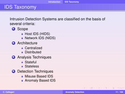
Intrusion Detection Systems are classified on the basis ofseveral criteria:
1 ScopeHost IDS (HIDS)Network IDS (NIDS)
2 ArchitectureCentralizedDistributed
3 Analysis TechniquesStatefulStateless
4 Detection TechniquesMisuse Based IDSAnomaly Based IDS
C. Callegari Anomaly Detection 11 / 169

Introduction IDS Taxonomy
Host based vs. Network based
Host based IDSAimed at detecting attacks related to a specific hostArchitecture/Operating System dependentProcessing of high level information (e.g. system calls)Effective in detecting insider misuse
Network based IDSAimed at detecting attacks towards hosts connected to aLANArchitecture/Operating System independentProcessing data at lower level of granularity (packets)Effective in detecting attacks from the “outside”
C. Callegari Anomaly Detection 12 / 169

Introduction IDS Taxonomy
Centralized IDS vs. Distributed IDS
Centralized IDSAll the operations are performed by the same machineMore simple to realizeOnly one point of failure
Distributed IDSComposed of several components
Sensors which generate security eventsConsole to monitor events and alerts and control the sensorsCentral Engine that records events and generate alarms
May need to deal with different data formatsNeed of a secure communication protocol (IPFIX)
C. Callegari Anomaly Detection 13 / 169

Introduction IDS Taxonomy
Stateless IDS vs. Stateful IDS
Stateless IDSTreats each event independently of the othersSimple system designHigh processing speed
Stateful IDSMaintains information about past eventsThe effect of a certain event depends on its position in theevents streamMore complex system designMore effective in detecting distributed attacks
C. Callegari Anomaly Detection 14 / 169

Introduction IDS Taxonomy
Misuse based IDS vs. Anomaly based IDS
Misuse based IDSIdentifies intrusion by looking for patterns of traffic or ofapplication data presumed to be maliciousPattern of misuses are stored in a databaseEffective in detecting only “known” attacks
Anomaly based IDSIdentifies intrusions by classifying activity as eitheranomalous or normalNeeds a training phase to recognize normal activityAble to detect “new” attacksGenerates more false alarms than a misuse based IDS
C. Callegari Anomaly Detection 15 / 169

Introduction IDS Taxonomy
Attacks State of the Art
C. Callegari Anomaly Detection 16 / 169

Introduction IDS Taxonomy
IDS State of the Art
Focus is on Network based IDSs (The only ones effectivein detecting Distributed Denial of Service - DDoS)State of the art IDSs are Misuse Based
Most attacks are realized by means of software toolsavailable on the InternetMost attacks are “well-known” attacks
BUT . . .. . . The most dangerous attacks are those written
ad hoc by the intruder!
C. Callegari Anomaly Detection 17 / 169

Introduction IDS Taxonomy
The best choice?
Combined use of bothHIDS (for insider attacks) & NIDS (for outsider attacks)Misuse IDS (low False Alarm rate) & Anomaly IDS (for“new” attacks)Stateless IDS (fast data process) & Stateful IDS (for“complex” attacks)
Distributed IDSNot a single point of failureMore effective in monitoring large networks
C. Callegari Anomaly Detection 18 / 169
Introduction IDS Taxonomy
The best choice?
C. Callegari Anomaly Detection 19 / 169

Introduction Some Useful Definitions
Definitions
False Positive (FP): the error of rejecting a null hypothesiswhen it is actually true. In our case it implies the creation ofan alarm in correspondence of normal activitiesFalse Negative (FN): the error of failing to reject a nullhypothesis when it is in fact not true. In our case itcorresponds to a missed detection
C. Callegari Anomaly Detection 20 / 169

Introduction Some Useful Definitions
ROC Curve
Plots Detection Rate vs. False Positive Rate
0 0.1 0.2 0.3 0.4 0.5 0.6 0.7 0.8 0.9 10
0.1
0.2
0.3
0.4
0.5
0.6
0.7
0.8
0.9
1
False Alarm Rate
Det
ectio
n R
ate
Non Stationary ECDFNon Homogeneous MCHomogeneous MC
C. Callegari Anomaly Detection 21 / 169

Introduction Some Useful Definitions
ROC Curve
Results presented by the ROC are often considered incompletebecause
they do not take into account the cost of missed attacksthey do not take into account the cost of false alarmsthey do not say if the system itself is resistant to attacks. . .
Several researchers are working on more complete ways ofrepresenting the results
C. Callegari Anomaly Detection 22 / 169

Introduction Evaluation Data-set
DARPA Evaluation Program
The 1998/1999 DARPA/MIT IDS evaluation program is themost comprehensive evaluation performed to dateIt provides a corpus of data for the development,improvement, and evaluation of IDSsDifferent kind of data are available:
Operating systems logsNetwork traffic
Collected by an “inside” snifferCollected by an “outside” sniffer
The data model the network traffic measured between aUS Air Force base and the Internet
C. Callegari Anomaly Detection 23 / 169

Introduction Evaluation Data-set
The DARPA Network
C. Callegari Anomaly Detection 24 / 169

Introduction Evaluation Data-set
The DARPA Dataset
5 weeks dataData from weeks 1 and 3 are attack free and can be usedto train the systemData from week 2 contains labeled attacks and can be usedto realize the signatures databaseData from weeks 4 and 5 contains several attacks and canbe used for the detection phase
An Attack Truth list is providedAttacks are categorized as
Denial of Service (DoS)User to Root (U2R)Remote to Local (R2L)DataProbe
177 instances of 59 different types of attacks
C. Callegari Anomaly Detection 25 / 169
Introduction Evaluation Data-set
Other Data-sets
The DARPA data-set has many drawbacks:simulated environmentnot up-to-date trafficthe methodology used for generating the traffic has beenshown to be inappropriate for simulating actual networks
Other Data-sets:several publicly available traffic tracese.g. CAIDA, Abilene (Internet2), GEANT, . . .no ground truth is provided!
C. Callegari Anomaly Detection 26 / 169

Introduction Evaluation Data-set
References
Anderson, Computer Security Monitoring andSurveillance, Tech Rep 98-17, 1980E. Millard , Internet attacks increase in number,severity, Top Tech News, 2005C. Staf , Hackers: companies encounter rise of cyberextortion, vol. 2006, Computer Crime Research Center,2005.S. Axelsson , Intrusion Detection Systems: A Surveyand Taxonomy, Chalmers University, Technical Report99-15, March 2000W. Stallings , Cryptography and Network Security,Prentice HallA. Patcha, J.M. Park , An overview of anomaly detectiontechniques: Existing solutions and latesttechnological trends, Computer Networks 51, 2008
C. Callegari Anomaly Detection 27 / 169

Introduction Evaluation Data-set
References
MIT, Lincoln laboratory, DARPA evaluation intrusiondetection, http://www.ll.mit.edu/IST/ideval/R. Lippmann, J. Haines, D. Fried, J. Korba, and K. Das ,The 1999 DARPA off-line intrusion detectionevaluation, Computer Networks 34, 2000J. Haines, R. Lippmann, D. Fried, E. Tran, S. Boswell, andM. Zissman , 1999 DARPA intrusion detection systemevaluation: Design and procedures, Tech. Rep. 1062,MIT Lincoln Laboratory, 2001J. McHugh, Testing Intrusion detection systems: acritique of the 1998 and 1999 DARPA intrusiondetection, ACM Transactions on Information and SystemSecurity 3, 2000Christian Callegari, Stefano Giordano, Michele Pagano,New Statistical Approaches for Anomaly Detection,Security and Communication Networks, to appear
C. Callegari Anomaly Detection 28 / 169

IDES
Outline
1 Introduction
2 Intrusion Detection Expert System
3 Statistical Anomaly Detection
4 Clustering
5 Markovian Models
6 Entropy-based Methods
7 Sketch
8 Principal Component Analysis
9 Wavelet Analysis
C. Callegari Anomaly Detection 29 / 169

IDES
A bit of History
The history of IDSs can be split in three main blocks1 First Generation IDSs (end of the 1970s)
The concept of IDS first appears in the 1970s and early1980s (Anderson, Computer Security Monitoring andSurveillance, Tech Rep 1980)Focus on audit data of a single machinePost processing of data
2 Second Generation IDSs (1987)Intrusion Detection Expert System (Denning, An intrusionDetection Model, IEEE Trans. on Soft. Eng., 1987)Statistical analysis of data
3 Third Generation IDSs (to come)Focus on the networkReal-time detectionReal-time reactionIntrusion Prevention System
C. Callegari Anomaly Detection 30 / 169

IDES
IDES
Model’s components
Subjects: initiators of activity on a target system
Objects: resources managed by the system files, commands,etc.
Audit Records: generated by the target system in response toactions performed or attempted by subjects
Profiles: structures that characterize the behavior of subjectswith respect to objects in terms of statistical metrics and modelsof observed activity
Anomaly Records: generated when abnormal behavior isdetected
Activity Rules: actions taken when some condition is satisfied
C. Callegari Anomaly Detection 31 / 169

IDES
Subjects and Objects
SubjectsInitiators of actions on the target systemIt is typically a terminal userThey can be grouped into different categories
Users groups may overlap
ObjectsReceptors of subjects’ actionsIf a subject is a recipient of actions (e.g. electronic mail), then isalso considered to be a objectAdditional structures may be imposed (e.g. records may begrouped in database)
Objects granularity depends on the environment
C. Callegari Anomaly Detection 32 / 169

IDES
Audit Records
{Subject, Action, Object, Exception-Condition,Resource-Usage, Time-stamp}
Action: operation performed by the subject on or with theobjectException-Condition: denotes which, if any, executioncondition is raised on the returnResource-Usage: list of quantitative elements, whereeach element gives the amount of some resourceTime-stamp: unique time/date stamp identifying when theaction took place
C. Callegari Anomaly Detection 33 / 169

IDES
Profiles
An activity profile characterizes the behavior of a givensubject (or set of subjects) with respect to a given object,thereby serving as a signature or description of normalactivity for its respective subject and objectObserved behavior is characterized in terms of a statisticalmetric and modelA metric is a random variable x representing a quantitativemeasure accumulated over a periodObservations xi of x obtained from the audit records areused together with a statistical model to determine whethera new observation is abnormalThe statistical models make no assumptions about theunderlying distribution of x ; all knowledge about x isobtained from the observations xi
C. Callegari Anomaly Detection 34 / 169
IDES
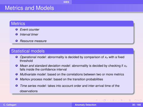
Metrics and Models
MetricsEvent counter
Interval timer
Resource measure
Statistical modelsOperational model : abnormality is decided by comparison of xn with a fixedthreshold
Mean and standard deviation model : abnormality is decided by checking if xnfalls inside the confidence interval
Multivariate model : based on the correlations between two or more metrics
Markov process model : based on the transition probabilities
Time series model : takes into account order and inter-arrival time of the
observations
C. Callegari Anomaly Detection 35 / 169

IDES
Profile structure
{Variable-name, Action-pattern, Exception-pattern,Resource-usage-pattern, Period, Variable-type, Threshold,
Subject-pattern, Object-pattern, Value}
Variable-nameAction-pattern: pattern that matches one or more actions in theaudit records (e.g. “login”)Exception-pattern: pattern that matches on theException-condition field of an audit recordResource-usage-pattern: pattern that matches on theResource-usage field of an audit recordPeriod: time interval for measurementsVariable-type: name of abstract data type that defines aparticular type of metric and statistical model (e.g. event counterwith mean and standard deviation model)Threshold
C. Callegari Anomaly Detection 36 / 169

IDES
Profile structure
{Variable-name, Action-pattern, Exception-pattern,Resource-usage-pattern, Period, Variable-type, Threshold,
Subject-pattern, Object-pattern, Value}
Subject-pattern: pattern that matches on the Subject fieldof an audit recordObject-pattern: pattern that matches on the Object field ofan audit recordValue: value of current observation and parameters usedby the statistical model to represent distribution of previousvalues
There also is the possibility of defining profiles for classes
C. Callegari Anomaly Detection 37 / 169

IDES
Profile templates
When user accounts and objects can be created dynamically, amechanism is needed to generate activity profiles for newsubjects and objects
Manual create: the security officer explicitly creates allprofilesAutomatic explicit create: all profiles for a new user aregenerated in response to a “create” record in the audit trailFirst use: a profile is automatically generated when asubject (new or old) first uses an object (new or old)
C. Callegari Anomaly Detection 38 / 169

IDES
Anomaly Records
{Event, Time-stamp, Profile}
Event: indicates the event giving rise to the abnormalityand is either “audit”, meaning the data in an audit recordwas found abnormal, or “period”, meaning the dataaccumulated over the current period was found abnormalTime-stamp: either the Time-stamp in the audit trail orinterval stop timeProfile: activity profile with respect to which theabnormality was detected
C. Callegari Anomaly Detection 39 / 169

IDES
Activity Rules
A condition that, when satisfied, causes the rule to be fired, anda body, which specified the action to be taken
Audit-record rule: triggered by a match between a new auditrecord and an activity profile, updates the profiles and checks foranomalous behavior
Periodic-activity-update rule: triggered by the end of aninterval matching the period component of an activity profile,updates the profiles and checks for anomalous behavior
Anomaly-record rule: triggered by the generation of ananomaly record, brings the anomaly to the immediate attentionof the security officer
Periodic-anomaly-analysis rule: triggered by the end of aninterval, generates summary reports of the anomalies during thecurrent period
C. Callegari Anomaly Detection 40 / 169

IDES
References
D. Denning , An intrusion detection model, IEEETransactions Software Engineering, vol. SE-13, no.2, 1987
C. Callegari Anomaly Detection 41 / 169

Statistical Anomaly Detection
Outline
1 Introduction
2 Intrusion Detection Expert System
3 Statistical Anomaly Detection
4 Clustering
5 Markovian Models
6 Entropy-based Methods
7 Sketch
8 Principal Component Analysis
9 Wavelet Analysis
C. Callegari Anomaly Detection 42 / 169

Statistical Anomaly Detection
Statistical Approach: Traffic Descriptors
The goal is to identify some traffic parameters, which can beused to describe the network traffic and that vary significantlyfrom the normal behavior to the anomalous one
Some examplesPacket lengthInter-arrival timeFlow sizeNumber of packets per flow. . . and so on
C. Callegari Anomaly Detection 43 / 169

Statistical Anomaly Detection
Choice of the Traffic Descriptors
For each parameter we can considerMean ValueVariance and higher order momentsDistribution functionQuantiles. . . and so on
The number of potential traffic descriptors is huge (somepapers identify up to 200 descriptors)
GOALTo identify as few “attack invariant” descriptors as possible to
classify traffic with an acceptable error rate
C. Callegari Anomaly Detection 44 / 169

Cluster
Outline
1 Introduction
2 Intrusion Detection Expert System
3 Statistical Anomaly Detection
4 ClusteringClusteringOutliers Detection
5 Markovian Models
6 Entropy-based Methods
7 Sketch
8 Principal Component Analysis
9 Wavelet AnalysisC. Callegari Anomaly Detection 45 / 169

Cluster Cluster
Clustering
Clustering is the assignment of a set of observations intosubsets (called clusters) so that observations in the samecluster are similar in some senseClustering is a method of unsupervised learningThe clusters are computed on the basis of a distancemeasure, which will determine how the similarity of twoelements is calculatedCommon distances are:
Euclidean distanceManhattan distanceMahalanobis distance. . .
C. Callegari Anomaly Detection 46 / 169

Cluster Cluster
K-Means Algorithm
The k-means algorithm assigns each point to the cluster whosecenter (also called centroid) is the nearest
1 Choose the number of clusters, k2 Randomly generate k clusters and determine the cluster
centers, or directly generate k random points as clustercenters
3 Assign each point to the nearest cluster center4 Recompute the new cluster centers5 Repeat the two previous steps until some convergence
criterion is met (e.g., the assignment hasn’t changed)
C. Callegari Anomaly Detection 47 / 169

Cluster Cluster
K-Means Algorithm - An example
Consider k = 2, choose 2 points (centroids), build 2 clusters
!"#$%&'($)*+(,-./01.),/,(2&$)*34
567%,.8&-($)*34)9,.'%&)&.)($8$)9-/1-",))))))46:"1/',%&;;&-($)&).$/'%&)8-'&)&.'$%.$)-)<1,/'&)9,.'%&
Figure Reproduced From “Data Analysis Tools for DNA Microarrays” by Sorin Draghici
C. Callegari Anomaly Detection 48 / 169

Cluster Cluster
K-Means Algorithm - An example
Compute the new centroids
!"#$%&'($)*+(,-./01.),/,(2&$)*34
56)7&8-"8$"&-($)&)8,.'%&)9-/-.:$8&)/1&).$/'%&)8"1/',%)8$%%,.'&
Figure Reproduced From “Data Analysis Tools for DNA Microarrays” by Sorin Draghici
C. Callegari Anomaly Detection 49 / 169

Cluster Cluster
K-Means Algorithm - An example
Build the new clusters
!"#$%&'($)*+(,-./01.),/,(2&$)345
67)8&9-::&-($)&"):"1/',%&.#);,&).$/'%&);-'&)&.'$%.$)-&).$/'%&).1$<&):,.'%&)
Figure Reproduced From “Data Analysis Tools for DNA Microarrays” by Sorin Draghici
C. Callegari Anomaly Detection 50 / 169

Cluster Cluster
K-Means Algorithm - An example
Repeat last 2 steps, until a assignments don’t change
!"#$%&'($)*+(,-./01.),/,(2&$)345
67)8&2,'&-($)#"&)1"'&(&)91,)2-//&):&.;<=);&)/$.$)21.'&);<,)
>,.#$.$)($//&)&.)1.)9&::,%,.',);"1/',%
Figure Reproduced From “Data Analysis Tools for DNA Microarrays” by Sorin Draghici
C. Callegari Anomaly Detection 51 / 169

Cluster Outliers Detection
Outliers
In statistics, an outlier is an observation that is numericallydistant from the rest of the dataDetection based on the full dimensional distances betweenthe points as well as the densities of local neighborhoodsThere exist at least two approaches
the anomaly detection model is trained using unlabeleddata that consist of both normal as well as attack trafficthe model is trained using only normal data and a profile ofnormal activity is created
C. Callegari Anomaly Detection 52 / 169

Cluster Outliers Detection
Outliers Detection - Method 1
The idea behind the first approach is that anomalous orattack data form a small percentage of the total dataAnomalies and attacks can be detected based on clustersizes
large clusters correspond to normal datathe rest of the data points, which are outliers, correspond toattacks
C. Callegari Anomaly Detection 53 / 169

Cluster Outliers Detection
References
L. Portnoy, E. Eskin, S.J. Stolfo , Intrusion detection withunlabeled data using clustering, ACM Workshop onData Mining Applied to Security, 2001S. Ramaswamy, R. Rastogi, K. Shim , Efficientalgorithms for mining outliers from large data sets,ACM SIGMOD International Conference on Managementof Data, 2000K. Sequeira, M. Zaki , ADMIT: Anomaly-based datamining for intrusions, ACM SIGKDD InternationalConference on Knowledge Discovery and Data Mining,2002V. Barnett, T. Lewis , Outliers in Statistical Data, Wiley,1994
C. Callegari Anomaly Detection 54 / 169

Cluster Outliers Detection
References
C.C. Aggarwal, P.S. Yu , Outlier detection for highdimensional data, ACM SIGMOD InternationalConference on Management of Data, 2001M. Breunig, H.-P. Kriegel, R.T. Ng, J. Sander , LOF:identifying density-based local outliers, ACM SIGMODInternational Conference on Management of Data, 2000E.M. Knorr, R.T. Ng , Algorithms for miningdistance-based outliers in large datasets, InternationalConference on Very Large Data Bases, 2008P.C. Mahalanobis , On tests and measures of groupsdivergence, Journal of the Asiatic Society of Bengal 26,1930
C. Callegari Anomaly Detection 55 / 169

Markovian Models
Outline
1 Introduction
2 Intrusion Detection Expert System
3 Statistical Anomaly Detection
4 Clustering
5 Markovian ModelsFirst Order Homogeneous Markov ChainsFirst Order Non Homogeneous Markov ChainsHigh Order Homogeneous Markov Chains
6 Entropy-based Methods
7 Sketch
8 Principal Component Analysis
9 Wavelet AnalysisC. Callegari Anomaly Detection 56 / 169

Markovian Models
State Transition Analysis
The approach was first proposed by Denning anddeveloped in the 1990s.Mainly used in two distinct environment
HIDS: to model the sequence of system commands usedby a userNIDS: to model the sequence of some specific fields of thepacket (e.g. the sequence of the flags values in a TCPconnection)
The most classical approach: Markov chains
C. Callegari Anomaly Detection 57 / 169

Markovian Models
Markov Chains and TCP
Idea: Model TCP connections by means of Markov chainsThe IP addresses and the TCP port numbers are used toidentify a connectionState space is defined by the possible values of the TCPflagsThe value of the flags is used to identify the chaintransitionsA value Sp is associated to each packet according to therule
Sp = syn + 2 · ack + 4 · psh + 8 · rst + 16 · urg + 32 · fin
C. Callegari Anomaly Detection 58 / 169

Markovian Models First Order Homogeneous Markov Chains
Markov Chain and TCP - Training phase
Calculate the transitionprobabilities
aij = P[qt+1 = j |qt = i] =
P[qt = i ,qt+1 = j]P[qt = i]
Server side3-way handshakepsh flagclosing
SSH Markov Chain
C. Callegari Anomaly Detection 59 / 169
Markovian Models First Order Homogeneous Markov Chains
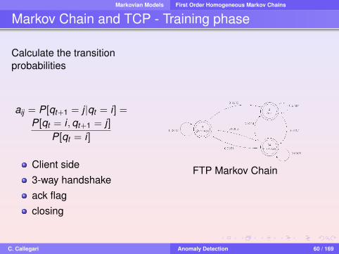
Markov Chain and TCP - Training phase
Calculate the transitionprobabilities
aij = P[qt+1 = j |qt = i] =
P[qt = i ,qt+1 = j]P[qt = i]
Client side3-way handshakeack flagclosing
FTP Markov Chain
C. Callegari Anomaly Detection 60 / 169

Markovian Models First Order Homogeneous Markov Chains
Markov Chain and TCP - Training phaseCalculate the transition probabilities
aij = P[qt+1 = j |qt = i] =
P[qt = i , qt+1 = j]P[qt = i]
SSH Markov Chain
3-WayHandshake
Syn FloodAttack
C. Callegari Anomaly Detection 61 / 169

Markovian Models First Order Homogeneous Markov Chains
Markov Chain and TCP - Detection phase
Given the observation (S1,S2, · · · ,ST )
The system has to decide between two hypothesis
H0 : normal behaviourH1 : anomaly
(1)
A possible statistic is given by the logarithm of theLikelihood Function
LogLF (t) =T+R∑
t=R+1
Log(aSt St+1)
Or by its temporal “derivative”
Dw (t) =
∣∣∣∣LogLF (t)− 1W
W∑i=1
LogLF (t − i)∣∣∣∣
C. Callegari Anomaly Detection 62 / 169

Markovian Models First Order Homogeneous Markov Chains
Markov Chain and TCP - Detection phase
C. Callegari Anomaly Detection 63 / 169

Markovian Models First Order Non Homogeneous Markov Chains
Non Homogeneous Markov Chain
First order homogeneous Markov chainP(Ct = si0 |Ct−1 = si1 ,Ct−2 = si2 ,Ct−3 = si3 , · · · ) =
P(Ct = si0 |Ct−1 = si1) = P(C0 = si0 |C−1 = si1) =
P(si0 |si1)
First order non-homogeneous Markov chainP(Ct = si0 |Ct−1 = si1 ,Ct−2 = si2 ,Ct−3 = si3 , · · · ) =
P(Ct = si0 |Ct−1 = si1) =
Pt(si0 |si1)
We build a distinct Markov Chain for each connection step(first 10 steps)The model should better characterizes the setup and therelease phases
C. Callegari Anomaly Detection 64 / 169

Markovian Models High Order Homogeneous Markov Chains
High order Markov Chain
First order homogeneous Markov chainP(Ct = si0 |Ct−1 = si1 ,Ct−2 = si2 ,Ct−3 = si3 , · · · ) =
P(Ct = si0 |Ct−1 = si1) = P(C0 = si0 |C−1 = si1) =
P(si0 |si1)
l th order homogeneous Markov chainP(Ct = si0 |Ct−1 = si1 ,Ct−2 = si2 ,Ct−3 = si3 , · · · ) =
P(Ct = si0 |Ct−1 = si1 ,Ct−2 = si2 , · · · ,Ct−l = sil ) =
P(C0 = si0 |C−1 = si1 ,C−2 = si2 , · · · ,C−l = sil ) =
P(si0 |si1 , si2 , · · · , sil )
Some connection phases have dependences, betweenpackets, of order bigger than 1
C. Callegari Anomaly Detection 65 / 169

Markovian Models High Order Homogeneous Markov Chains
Mixture Transition Distribution
We have an explosion of the number of the chainparameters, which grows exponentially with the order(K l(K − 1))Parsimonious representation of the transition probabilitiesMixture Transition Distribution (MTD) model(K (K − 1) + l − 1)
P(Ct = si0 |Ct−1 = si1 ,Ct−2 = si2 , · · · ,Ct−l = sil ) =lX
j=1
λj r(si0 |sij )
where the quantitiesR = {r(si |sj); i , j = 1, 2, · · · ,K} and Λ = {λj ; j = 1, 2, · · · , l}
satisfy the constraints
r(si |sj) ≥ 0; i , j = 1, 2, · · · ,K andKX
si =1
r(si |sj) = 1 ∀j = 1, 2, · · · ,K
λj ≥ 0; j = 1, 2, · · · , llX
j=1
λj = 1
C. Callegari Anomaly Detection 66 / 169

Markovian Models High Order Homogeneous Markov Chains
State Space Reduction
We only consider the states observed during the trainingphaseWe add a rare state to take into account all the otherpossible statesWe fix the following quantities:
r(rare|si) = ε ∀i = 1,2, · · · ,Kwith ε small (in our case ε = 10−6)
r(si |rare) = (1− ε)/(K − 1)
∀i = 1,2, · · · ,K − 1 (2)
C. Callegari Anomaly Detection 67 / 169

Markovian Models High Order Homogeneous Markov Chains
Parameters Estimation
We need to estimate the parameters of the Markov chain(Maximum Likelihood Estimation - MLE)According to the MTD model, the log-likelihood of asequence (c1, c2, · · · , cT ) of length T is:
LL(c1, c2, · · · , cT ) =K∑
i0=1
· · ·K∑
il=1
N(si0 , si1 , · · · , sil )·log( l∑
j=1
λj r(si0 |sij )
)
where N(si0 , si1 , · · · , sil ) represents the number of timesthe transition sil → sil−1 → · · · → si0 is observedWe have to maximize the right hand side of the equation,with respect to R and Λ, taking into account the givenconstraints
C. Callegari Anomaly Detection 68 / 169

Markovian Models High Order Homogeneous Markov Chains
Parameters Estimation
Estimation StepsWe apply an alternate maximization with respect to R andto Λ
In the first step (estimation of Λ) we use the sequentialquadratic programmingThe second step (estimation of R) is a linear inverseproblem with positivity constraints (LININPOS) that wesolve applying the Expectation Maximization (EM)algorithm
Global MaximumThis process leads to a global maximum,
since LL is concave in R and Λ.
C. Callegari Anomaly Detection 69 / 169

Markovian Models High Order Homogeneous Markov Chains
Markov Chains - Detection Phase
Choose between a single hypothesis H0 (estimatedstochastic model), and the composite hypothesis H1 (allthe other possibilities)
H0 : {(c1, c2, · · · , cT ) ∼ computed model MC0}
H1 : {anomaly}
No optimal result is presented in the literatureThe best solution is represented by the use of theGeneralized Likelihood Ratio (GLR) test:
X =
(Maxv 6=uL(c1, c2, · · · , cT |Λv ,Rv )
L(c1, c2, · · · , cT |Λu,Ru)
)1T H0
≶H1
ξ
C. Callegari Anomaly Detection 70 / 169

Markovian Models High Order Homogeneous Markov Chains
Markov Chains - Detection Phase
Equivalent to decide on the basis of the Kullback-Leiblerdivergence between the model associated to H0 (MC0) and theone computed for the observed sequence (MCs)
The Kullback-Leibler divergence, for first order Markov chains, isdefined as:
KL (MC0,MCs) =∑
i
∑j
π0(si )P0(sj |si ) logP0(sj |si )
Ps(sj |si )
where π0(si ) is the stationary distribution of MC0 and Pk (sj |si ) isthe (single step) transition probability from state Ct−1 = si tostate Ct = sj
Extension to Markovian models of order lThe state of the chain Ct has to be considered as a point in a finitel-dimensional lattice:
Ct = (Ct ,Ct−1, . . .,Ct−l+1)
C. Callegari Anomaly Detection 71 / 169

Markovian Models High Order Homogeneous Markov Chains
Non-Homogeneous Markov Chain
0 0.1 0.2 0.3 0.4 0.5 0.6 0.7 0.8 0.9 10
0.1
0.2
0.3
0.4
0.5
0.6
0.7
0.8
0.9
1
False Alarm Rate
Det
ectio
n R
ate
Non Stationary ECDFNon Homogeneous MCHomogeneous MC
C. Callegari Anomaly Detection 72 / 169

Markovian Models High Order Homogeneous Markov Chains
High Order Markov Chain
C. Callegari Anomaly Detection 73 / 169

Markovian Models High Order Homogeneous Markov Chains
References
N. Ye, Y.Z.C.M Borror, Robustness of the Markov-chainmodel for cyber-attack detection, IEEE Transactions onReliability 53, 2004D.-Y. Yeung, Y. Ding , Host-based intrusion detectionusing dynamic and static behavioral models, PatternRecognition 36, 2003W.-H. Ju and Y. Vardi , A hybrid high-order Markov chainmodel for computer intrusion detection, Tech. Rep. 92,NISS, 1999M. Schonlau, W. DuMouchel, W.-H. Ju, A. Karr, M. Theus,and Y. Vardi , Computer intrusion: Detectingmasquerades, Tech. Rep. 95, NISS, 1999N. Ye, T. Ehiabor, and Y. Zhanget , First-order versushigh-order stochastic models for computer intrusiondetection, Quality and Reliability EngineeringInternational, vol. 18, 2002
C. Callegari Anomaly Detection 74 / 169

Markovian Models High Order Homogeneous Markov Chains
References
A. Raftery , A model for high-order markov chains,Journal of the Royal Statistical Society, series B, vol. 47,1985A. Raftery and S. Tavare , Estimation and modellingrepeated patterns in high-order markov chains with themixture transition distribution (MTD) model, Journal ofthe Royal Statistical Society, series C - Applied Statistics,vol. 43, 1994Y. Vardi and D. Lee , From image deblurring to optimalinvestments: Maximum likelihood solutions forpositive linear inverse problem, Journal of the RoyalStatistical Society, series B, vol. 55, 1993C. Callegari, S. Vaton, and M. Pagano , A new statisticalapproach to network anomaly detection, PerformanceEvaluation of Computer and Telecommunication Systems(SPECTS), 2008
C. Callegari Anomaly Detection 75 / 169

Entropy
Outline
1 Introduction
2 Intrusion Detection Expert System
3 Statistical Anomaly Detection
4 Clustering
5 Markovian Models
6 Entropy-based MethodsEntropyCompression Algorithms
7 Sketch
8 Principal Component Analysis
9 Wavelet AnalysisC. Callegari Anomaly Detection 76 / 169

Entropy Entropy
Theoretical Background
EntropyThe entropy H of a discrete random variable X is a measure ofthe amount of uncertainty associated with the value of XReferring to an alphabet composed of n distinct symbols,respectively associated to a probability pi , then
H = −n∑
i=1
pi · log2pi bit/symbol
The starting pointThe entropy represents a lower bound to the compression ratethat we can obtain: the more redundant the data are and thebetter we can compress them.
C. Callegari Anomaly Detection 77 / 169

Entropy Compression Algorithms
Compression Algorithms
Dictionary based algorithms: based on the use of adictionary, which can be static or dynamic, and they codeeach symbol or group of symbols with an element of thedictionary
Lempel-Ziv-Welch (LZW)Model based algorithms: each symbol or group ofsymbols is encoded with a variable length code, accordingto some probability distribution.
Huffman Coding (HC)Dynamic Markov Compression (DMC)
C. Callegari Anomaly Detection 78 / 169

Entropy Compression Algorithms
Lempel-Ziv-Welch
Created by Abraham Lempel, Jacob Ziv, and Terry Welch.It was published by Welch in 1984 as an improvedimplementation of the LZ78 algorithm, published byLempel and Ziv in 1978Universal adaptative1 lossless data compression algorithmBuilds a translation table (also called dictionary) from thetext being compressedThe string translation table maps the message strings tofixed-length codes
1The coding scheme used for the k th character of a message is based onthe characteristics of the preceding k − 1 characters in the message
C. Callegari Anomaly Detection 79 / 169

Entropy Compression Algorithms
Huffman Coding
Developed by Huffman (1952)Based on the use of a variable-length code table forencoding each source symbolThe variable-length code table is derived from a binary treebuilt from the estimated probability of occurrence for eachpossible value of the source symbolsPrefix-free code2 that expresses the most commoncharacters using shorter strings of bits than are used forless common source symbols
2The bit string representing some particular symbol is never a prefix of thebit string representing any other symbol
C. Callegari Anomaly Detection 80 / 169

Entropy Compression Algorithms
Dynamic Markov Compression
Developed by Gordon Cormack and Nigel Horspool (1987)Adaptative lossless data compression algorithmBased on the modelization of the binary source to beencoded by means of a Markov chain, which describes thetransition probabilities between the symbol “0” and thesymbol “1”The built model is used to predict the future bit of amessage. The predicted bit is then coded using arithmeticcoding
C. Callegari Anomaly Detection 81 / 169

Entropy Compression Algorithms
System Design
InputThe system input is given by raw traffic traces in libpcapformatThe 5-tuple is used to identify a connection, while the valueof the TCP flags is used to build the “profile”A value si is associated to each packet:
si = SYN +2 ·ACK +4 ·PSH +8 ·RST +16 ·URG +32 ·FIN
thus each “mono-directional” connection is represented bya sequence of symbols si , which are integers in{0,1, · · · ,63}
C. Callegari Anomaly Detection 82 / 169

Entropy Compression Algorithms
System Design
Training Phase
Choose one of the three previously described algorithms(Huffman, DMC, or LZW)The compression algorithms have been modified so as thatthe “learning phase” is stopped after the training phase:
Huffman case: the occurency frequency of each symbol isestimated only on the training datasetDMC case: the estimation of the Markov chain is onlyupdated during the training phaseLZW case: the construction of the dictionary is stoppedafter the training phase
Detection performed with a compression scheme that is“optimal” for the “normal” traffic used for building theconsidered “profile” and suboptimal for “anomalous” traffic
C. Callegari Anomaly Detection 83 / 169

Entropy Compression Algorithms
System Design
Detection PhaseAppend each distinct “observed” connection b, to thetraining sequence ACompute the “compression rate per symbol”:
X =dim([A|b]∗)− dim([A]∗)
Length(b)
where [X ]∗ represents the compressed version of XChoose between a single hypothesis H0 (normal traffic),and the composite hypothesis H1 (anomaly)
XH0≶H1
ξ
C. Callegari Anomaly Detection 84 / 169
Entropy Compression Algorithms
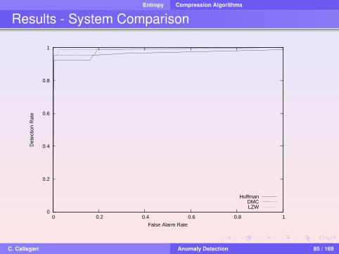
Results - System Comparison
0
0.2
0.4
0.6
0.8
1
0 0.2 0.4 0.6 0.8 1
Det
ectio
n R
ate
False Alarm Rate
HuffmanDMCLZW
C. Callegari Anomaly Detection 85 / 169

Entropy Compression Algorithms
Results - On-line System
0
0.2
0.4
0.6
0.8
1
0 0.2 0.4 0.6 0.8 1
Dete
ctio
n Ra
te
False Alarm Rate
HuffmanDMCLZW
C. Callegari Anomaly Detection 86 / 169

Entropy Compression Algorithms
References
T. Cover and J. Thomas , Elements of informationtheory, Wiley-Interscience, 2nd ed., 2006C. E. Shannon , A mathematical theory ofcommunication, Bell System Technical Journal, vol. 271948D. Huffman , A method for the construction ofminimum-redundancy codes, Proceedings of theInstitute of Radio Engineers, vol. 40, 1952G. Cormack and N. Horspool , Data compression usingdynamic Markov modelling, vol. 30, 1987
C. Callegari Anomaly Detection 87 / 169

Entropy Compression Algorithms
References
J. Ziv and A. Lempel , Compression of individualsequences via variable-rate coding, IEEE Transactionson Information Theory, vol. 24, 1978T. Welch , A technique for high-performance datacompression, IEEE Computer Magazine, vol. 17, no. 6,1984Christian Callegari, Stefano Giordano, Michele Pagano ,On the Use of Compression Algorithms for NetworkAnomaly Detection, IEEE International Conference onCommunications (ICC 2009)
C. Callegari Anomaly Detection 88 / 169

Sketch
Outline
1 Introduction
2 Intrusion Detection Expert System
3 Statistical Anomaly Detection
4 Clustering
5 Markovian Models
6 Entropy-based Methods
7 SketchCount-Min sketchHeavy Hitters Detection
8 Principal Component Analysis
9 Wavelet AnalysisC. Callegari Anomaly Detection 89 / 169

Sketch Count-Min sketch
Data Stream Mining
Data Stream miningThe data stream mining is a set of techniques which permits toanalyze a data flow, almost in real-time, without storing all thedata
Can be used to analyze, for example, the network trafficThe aim can be the calculation of histograms, theindividuation of the most common features, etc.Two constraints
1 Almost real-time2 Without storing all the data
C. Callegari Anomaly Detection 90 / 169

Sketch Count-Min sketch
The Count-Min Sketch Algorithm
Proposed by Cormode and Muthukrishran, 2004Each element of the data flow is identified by
id it ∈ {1,2, . . . ,N}, with N biglabel ct ∈ R
The data flow is the sequence (it , ct )t∈NAn example
The data flow is the network trafficit is the source IP address of packet tct is the length of packet t
C. Callegari Anomaly Detection 91 / 169

Sketch Count-Min sketch
The Count-Min Sketch Algorithm
At each instant τ ∈ N and for each id i , we define a countai(τ)
ai(τ)def=
τ∑t=0
ctδi,it
with δi,it = 1 if i = it and δi,it = 0 otherwise
In our example ai(τ) is the total number of bytes sent fromi up to the instant τFirst step of the algorithm: estimate ai(τ)
C. Callegari Anomaly Detection 92 / 169

Sketch Count-Min sketch
The Count-Min Sketch Algorithm
Fix the precision ε and the failure probability δLet’s w = de
ε e and d = dln 1δ e
Let’s take d independent random hash functionsLet’s allocate a table Countdxw initialized to zeroFor each instant t , let’s update the table according to:for eachj ∈ {1,2, . . . ,d} Count [j ,hj(it )] = Count [j ,hj(it )] + ct
C. Callegari Anomaly Detection 93 / 169

Sketch Count-Min sketch
The Count-Min Sketch Algorithm
At the instant τ and for each id i ∈ {1,2, . . . ,N} we have anestimation ai(τ) of the count ai(τ)
ai(τ) = minj
Count [j ,hj(it )](τ)
C. Callegari Anomaly Detection 94 / 169

Sketch Count-Min sketch
The Count-Min Sketch Algorithm
Main propertiesThe estimator ai(τ) ≥ ai(τ)
P{ai(τ) ≤ ai(τ) + ε||−→a (τ)||1} ≥ 1− δ−→a (τ)
def= (a1(τ),a2(τ), . . . ,aN(τ))
||−→a (τ)||1def= |a1(τ)|+ |a2(τ)|+ . . .+ |aN(τ)|
C. Callegari Anomaly Detection 95 / 169

Sketch Count-Min sketch
The Count-Min Sketch Algorithm
Complexity in timeNumber of operations for updating the Count table isO(ln(1
δ ))
Number of operations for calculating ai is O(ln(1δ ))
Complexity in spaceNumber of words for storing the hash functions and theCount table is O(1
ε ln(1δ ))
C. Callegari Anomaly Detection 96 / 169

Sketch Heavy Hitters Detection
Finding Heavy Hitters
Aim: find those items whose frequencies exceed athreshold φ during the observation windowThese items are called Heavy HittersPossible application: finding the IP addresses, whosecontribution to the network traffic exceeds the thresholdAn anomaly can be detected as a variation of the heavyhitters distribution
At a given instant τ and for a given threshold φ we define heavyhitters all the i , such that ai(τ) ≥ φ ‖ ~a(τ) ‖1
C. Callegari Anomaly Detection 97 / 169

Sketch Heavy Hitters Detection
Application of the Count-Min sketch algorithm
Initialization, at the instant t = 0
Calculate ‖ ~a(0) ‖1= c0
Update CountAdd i0 and his estimated count ai0(0) to the list L of thepotential heavy hitters
C. Callegari Anomaly Detection 98 / 169

Sketch Heavy Hitters Detection
Application of the Count-Min sketch algorithm
Iteration, at the instant t = t
Calculate ‖ ~a(t) ‖1=‖ ~a(t − 1) ‖1 +ct
Update CountCalculate the estimated count ait (t)If ait (t) ≥ φ ‖ ~a(t) ‖1 then
If it does not belongs to L: add it and his estimated countait (t) to LElse replace the count corresponding to it
Eliminate from the list every i , whose count is less thanφ ‖ ~a(t) ‖1
After all the iterations, L contains all the heavy hittersThe real count of all the elements of L is greater than(φ− ε) ‖ ~a(t) ‖1, with probability at least 1− δ
C. Callegari Anomaly Detection 99 / 169

Sketch Heavy Hitters Detection
Finding Hierarchical Heavy Hitters
Extension of the method, which takes into account thehierarchical structure of the IP addressesThe Hierarchical Heavy Hitters (HHH) are definedrecursively from the bottom to the top of the hierarchyAt the lowest level (level 0), the HHH are the Heavy Hitters(i.e all those source addresses whose counts exceed thethreshold)At level l > 0 an IP prefix is a HHH if its count minus thecount of its descendant HHHs is greater that or equal tothe threshold
C. Callegari Anomaly Detection 100 / 169

Sketch Heavy Hitters Detection
Finding Hierarchical Heavy Hitters
C. Callegari Anomaly Detection 101 / 169

Sketch Heavy Hitters Detection
References
Graham Cormode, S. Muthukrishnan , An Improved DataStream Summary: The Count-Min Sketch and itsApplications, Theoretical Informatics, 2004Pascal Cheung-Mon-Chan et al , Finding HierarchicalHeavy Hitters with the Count Min Sketch, IPS-MOME2006
C. Callegari Anomaly Detection 102 / 169

PCA
Outline
1 Introduction
2 Intrusion Detection Expert System
3 Statistical Anomaly Detection
4 Clustering
5 Markovian Models
6 Entropy-based Methods
7 Sketch
8 Principal Component AnalysisPCADetection and Identification
9 Wavelet AnalysisC. Callegari Anomaly Detection 103 / 169

PCA PCA
Principal Component Analysis
PCA is a coordinate transformation method that maps themeasured data onto a new set of axes
These axes are called Principal ComponentsEach principal component points in the direction ofmaximum variation or energy remaining in the dataThe principal axes are ordered by the amount of energy inthe data they capture
C. Callegari Anomaly Detection 104 / 169

PCA PCA
Geometric illustration
C. Callegari Anomaly Detection 105 / 169

PCA PCA
Data
A week of network-wide traffic measurements from Internet2:Internet2 samples 1 out of every 100 packets for inclusionin the flow statisticsIn Internet2 packets are aggregated into five-minutetime-binsAbilene anonymizes the last eleven bits of the IP addressstored in the flow records
Routing Info.
In order to aggregate the collected IP flows into OD flows, wealso need to parse the routing data. Internet2 deploys ZebraBGP monitors that record all BGP messages they receive.
C. Callegari Anomaly Detection 106 / 169

PCA PCA
Data
Measurements Matrix,Xt×p:
Let p denote the number of traffic aggregate
Let t denote the number of time-bin
Column i denotes the time-series of the i-th traffic aggregate,with zero mean
Row j represents an instance of all the traffic aggregate at j-thtime-bin
x , transposed row of X
X =
x11 x12 · · · x1px21 x22 · · · x2p...
.... . .
...xt1 xt2 · · · xtp
C. Callegari Anomaly Detection 107 / 169

PCA PCA
Principal Component Analysis
Using PCA, we find that the set of OD flows has small intrinsicdimension (10 or less)
Stability over time of this kind of representation (from week to week)
Origin Destination Flows
An OD flow consists of all traffic entering the network at a given point,and exiting the network at some other point, this is one out of thethree traffic aggregations analyzed.
High dimensional multivariate structure
PCA: lower dimensional approximation
C. Callegari Anomaly Detection 108 / 169

PCA PCA
Principal Component Analysis
Generalization of PCA to higher dimensions, as in the caseof X , take the rows of X as points in Euclidean space, sothat we have a dataset of t points in Rp
Mapping the data onto the first r principal axes places thedata into an r -dimensional hyperplane.
C. Callegari Anomaly Detection 109 / 169

PCA PCA
Linear algebraic formulation
Calculating the principal components is equivalent tosolving the symmetric eigenvalue problem for the matrixX T XEach principal component vi is the i-th eigenvectorcomputed from the spectral decomposition of X T X :
X T Xvi = λivi i = 1, . . .p (3)
Where λi is the eigenvalue corrisponding to vi
k -th principal component:
vk = arg max||v ||=1
||(X −k−1∑i=1
XvivTi )v ||
C. Callegari Anomaly Detection 110 / 169

PCA PCA
Principal Component Analysis
Once the data have been mapped into principal componentspace, it can be useful to examine the transformed data onedimension at a time:
The contribution of principal axis i as a function of time is givenby Xvi
This vector can be normalized to unit length by dividing byσi =
√λi
Thus, we have for each principal axis i :
ui =Xvi
σii = 1, . . . ,p (4)
The ui (eigenflows) are vectors of size t and orthogonal by construction
C. Callegari Anomaly Detection 111 / 169

PCA PCA
Principal Component Analysis
Thus vector ui captures the temporal variation common toall flows along principal axis iThe set of principal components {vi}pi=1 can be arranged inorder as columns of a principal matrix Vp×p
Likewise we can form the matrix Ut×p in which column i isui
Then taken together, V , U, and σi can be arranged towrite each traffic aggregate Xi as:
Xi
σi= U(V T )i i = 1, . . . ,p (5)
Xi is the time-series of the i-th traffic aggregate and (V T )i is the i-th row of V
C. Callegari Anomaly Detection 112 / 169

PCA PCA
Principal Component Analysis
Equation 5 makes clear that each traffic aggregate Xi is in turna linear combination of the ui , with associated weights (V T )i
The elements of {σi}ki=1 are the singular values
||Xvi || = vTi X T Xvi = λivT
i vi = λi (6)
Thus, the singular values are useful for gauging thepotential for reduced dimensionality in the data, oftensimply through their visual examination in a scree plot
C. Callegari Anomaly Detection 113 / 169

PCA PCA
Scree Plot
Energy Percentages captured by first PCs
C. Callegari Anomaly Detection 114 / 169

PCA PCA
Lower Dimensional Approximation
Finding that only r singular values are non-negligible,implies that X effectively resides on an r -dimensionalsubspace of Rp:
X ′ ≈r∑
i=1
σiuivi (7)
where r < p is the effective intrinsic dimension of X
C. Callegari Anomaly Detection 115 / 169

PCA Detection and Identification
Subspace Method
Subspace MethodThis method is based on a separation of the high-dimensionalspace occupied by a set of network traffic measurements intodisjoint subspaces corresponding to normal and anomalousnetwork conditions.
This separation can be performed effectively by PrincipalComponent AnalysisOnce the principal axes have been determined, thedata-set can be mapped onto the new axes
1 Normal subspace: S2 Anomalous Subspace: S
C. Callegari Anomaly Detection 116 / 169

PCA Detection and Identification
Modeled and Residual Part of x
Detecting volume anomalies in link traffic relies on theseparation of link traffic x at any time-step into normal andanomalous components:
1 modeled part of x2 residual part of x
We seek to decompose the set of link measurements at a givenpoint in time x :
x = x + x
We form x by projecting x onto S, and we form x by projecting x onto S
C. Callegari Anomaly Detection 117 / 169

PCA Detection and Identification
Anomalous Subspace
Anomalous Subspace, xTo accomplish this, we arrange the set of principal componentscorresponding to the normal subspace (v1, v2, . . . , vr ) ascolumns of a matrix P of size m × r where r denotes thenumber of normal axes.
x = PPT x = Cx and x = (I − PPT )x = Cx
C. Callegari Anomaly Detection 118 / 169

PCA Detection and Identification
Squared Prediction Error
A useful statistic for detecting abnormal changes in x is theSquared Prediction Error (SPE):
SPE = ||x ||2 = ||Cx ||2
and we may consider network traffic to be normal if:
SPE ≤ threshold
C. Callegari Anomaly Detection 119 / 169

PCA Detection and Identification
Identification
Now we know the anomalous time binWe don’t know which is the anomalous traffic aggregateresponsible for this anomaly
Identification, for every ||x ||2 over the threshold:
We determine the smallest set of OD flows, which if removedfrom the corresponding statistic, would bring it under threshold.
C. Callegari Anomaly Detection 120 / 169

PCA Detection and Identification
Multiway Subspace Method
The distributions of packet features (IP addresses andports) observed in flow traces reveal both the presenceand the structure of a wide range of anomalies.They enable highly sensitive detection of a wide range ofanomaliesTraffic Features:
1 Src IP2 Dest IP3 Src Port4 Dest Port
C. Callegari Anomaly Detection 121 / 169

PCA Detection and Identification
Features Distributions
Many important kinds of traffic anomalies cause changesin the distribution of addresses or ports observed in trafficHow feature distributions change as the result of a trafficanomaly (e.g., port scan)
5 10 15 20 25 30 35 400
5
10
15
20
25
30
Destination Port Rank
# of
Pac
kets
50 100 150 200 250 300 350 400 450 500
5
10
15
20
25
30
Destination Port Rank
# of
Pac
kets
5 10 15 20 25 30 35 40 45 500
5
10
15
20
25
30
Destination IP Rank
# of
Pac
kets
5 10 15 20 25 30 35 40 45 50
50
100
150
200
250
300
350
400
450
500
Destination IP Rank
# of
Pac
kets
(a) Normal (b) During Anomaly
Figure 1: Distribution changes induced by a port scan anomaly.Upper: dispersed destination ports; lower: concentrated desti-nation IPs.
where is the total number of observations in the his-togram. The value of sample entropy lies in the range .The metric takes on the value 0 when the distribution is maximallyconcentrated, i.e., all observations are the same. Sample entropytakes on the value when the distribution is maximally dis-persed, i.e.,Sample entropy can be used as an estimator for the source en-
tropy of an ergodic stochastic process. However it is not our intenthere to use sample entropy in this manner. We make no assump-tions about ergodicity or stationarity in modeling our data. We sim-ply use sample entropy as a convenient summary statistic for a dis-tribution’s tendency to be concentrated or dispersed. Furthermore,entropy is not the only metric that captures a distribution’s concen-tration or dispersal; however we have explored other metrics andfind that entropy works well in practice.In this paper we compute the sample entropy of feature distribu-
tions that are constructed from packet counts. The range of valuestaken on by sample entropy depends on the number of distinctvalues seen in the sampled set of packets. In practice we find thatthis means that entropy tends to increase when sample sizes in-crease, i.e., when traffic volume increases. This has a number ofimplications for our approach. In the detection process, it meansthat anomalies showing unusual traffic volumes will also some-times show unusual entropy values. Thus some anomalies detectedon the basis of traffic volume are also detected on the basis of en-tropy changes. In the classification process, the effect of this phe-nomenon is mitigated by normalizing entropy values as explainedin Section 4.3.Entropy is a sensitive metric for detecting and classifying
changes in traffic feature distributions. Later (Section 7.2.2) wewill show that each of the anomalies in Table 1 can be classified byits effect on feature distributions. Here, we illustrate the effective-ness of entropy for anomaly detection via the example in Figure 2.The figure shows plots of various traffic metrics around the time
of the port scan anomaly whose histograms were previously shownin Figure 1. The timepoint containing the anomaly is marked witha circle. The upper two timeseries show the number of bytes andpackets in the origin-destination flow containing this anomaly. The
0.51
1.52
x 106
# By
tes
5001000150020002500
# Pa
cket
s
0.51
1.52
2.5x 10⁻³
H(D
st IP
)
12/19 12/20
1
2
3x 10⁻³
H(D
st P
ort)
Figure 2: Port scan anomaly viewed in terms of traffic volumeand in terms of entropy.
lower two timeseries show the values of sample entropy for desti-nation IP and destination port. The upper two plots show that theport scan is difficult to detect on the basis of traffic volume, i.e., thenumber of bytes and packets in 5 minute bins. However, the lowertwo plots show that the port scan stands out clearly when viewedthrough the lens of sample entropy. Entropy of destination IPs de-clines sharply, consistent with a distributional concentration arounda single address, and entropy of destination ports rises sharply, con-sistent with a dispersal in the distribution of observed ports.
4. DIAGNOSIS METHODOLOGYOur anomaly diagnosis methodology leverages these observa-
tions about entropy to detect and classify anomalies. To detectanomalies, we introduce the multiway subspace method, and showhow it can be used to detect anomalies across multiple traffic fea-tures, and across multiple Origin-Destination (or point to point)flows. To classify anomalies, we adopt an unsupervised classifica-tion strategy and show how to cluster structurally similar anomaliestogether. Together, the multiway subspace method and the clus-tering algorithms form the foundation of our anomaly diagnosismethodology.
4.1 The Subspace MethodBefore introducing the multiway subspace method, we first re-
view the subspace method itself.The subspace method was developed in statistical process con-
trol, primarily in the chemical engineering industry [7]. Its goal isto identify typical variation in a set of correlated metrics, and detectunusual conditions based on deviation from that typical variation.Given a data matrix in which columns represent variables
or features, and rows represent observations, the subspace methodworks as follows. In general we assume that the features showcorrelation, so that typical variation of the entire set of features canbe expressed as a linear combination of less than variables. Usingprincipal component analysis, one selects the new set ofvariables which define an -dimensional subspace. Then normalvariation is defined as the projection of the data onto this subspace,and abnormal variation is defined as any significant deviation of thedata from this subspace.In the specific case of network data, this method is motivated by
results in [25] which show that normal variation of OD flow traffic
220
C. Callegari Anomaly Detection 122 / 169

PCA Detection and Identification
Entropy
The distribution of traffic features is a high-dimensional objectand so can be difficult to work with directly.
1 Analyze the degree of dispersal or concentration of thedistribution
2 A metric that captures the degree of dispersal orconcentration of a distribution is sample entropy
3 Empirical histogram Y = {ni , i = 1, . . . ,N}4 Sample entropy:
H(Y ) = −N∑
i=1
ni
Slog2
ni
S
where S =PN
i=1 ni is the total number of observations in the histogram
C. Callegari Anomaly Detection 123 / 169

PCA Detection and Identification
Multiway Anomalies
Anomalies typically induce changes in multiple traffic features.
Figure 3: Multivariate, multi-way data to analyze.
is well described as occupying a low dimensional space. This lowdimensional space is called the normal subspace, and the remainingdimensions are called the residual subspace.Having constructed the normal and residual subspaces, one can
decompose a set of traffic measurements at a particular point intime, , into normal and residual components: Thesize ( norm) of is a measure of the degree to which the par-ticular measurement is anomalous. Statistical tests can then beformulated to test for unusually large , based on setting a de-sired false alarm rate [13].The separation of features into distinct subspaces can be accom-
plished by various methods. For our datasets (introduced in Sec-tion 5), we found a knee in the amount of variance captured at
(which accounted for 85% of the total variance); we there-fore used the first 10 principal components to construct the normalsubspace.
4.2 The Multiway Subspace MethodWe introduce the multiway subspace method in order to address
the following problem. As shown in Table 1, anomalies typicallyinduce changes in multiple traffic features. To detect an anomaly inan OD flow, we must be able to isolate correlated changes (positiveor negative) across all its four traffic features (addresses and ports).Moreover, multiple OD flows may collude to produce network-wide anomalies. Therefore, in addition to analyzing multiple trafficfeatures, a detection method must also be able to extract anomalouschanges across the ensemble of OD flows.A visual representation of this multiway (spanning multiple traf-
fic features) and multivariate (spanning mulitple OD flows) data ispresented in Figure 3. There are four matrices, one for each traf-fic feature. Each matrix represents the multivariate timeseries of aparticular metric for the ensemble of OD flows in the network.Let denote the three-way data matrix in Figure 3. is com-
posed of the multivariate entropy timeseries of all the OD flows,organized by distinct feature matrices; denotes the en-tropy value at time for OD flow , of the traffic feature . Wedenote the individual matrices by srcIP , dstIP , srcPort ,and dstPort . Each matrix is of size , and contains the en-tropy timeseries of length bins for OD flows for a specific trafficfeature. Anomalous values in any feature and any OD flow corre-spond to outliers in this multiway data; the task at hand is to minefor outliers in .The multiway subspace method draws on ideas that have been
well studied in multivariate statistics [16]. An effective way ofanalyzing multiway data is to recast it into a simpler, single-wayrepresentation. The idea behind the multiway subspace method isto “unfold” the multiway matrix in Figure 3 into a single, large ma-
trix. And, once this transformation from multiway to single-wayis complete, the subspace method (which in general is designedfor single-way data [23]) can be applied to detect anomalies acrossdifferent OD flows and different features.We unwrap by arranging each individual feature matrix side
by side. This results in a new, merged matrix of size , whichcontains the ensemble of OD flows, organized in submatrices forthe four traffic features. We denote this merged matrix by . Thefirst columns of represent the source IP entropy submatrix ofthe ensemble of OD flows. The next columns (from column
to ) of contain the source port submatrix, followed by thedestination IP submatrix (columns to ) and the destinationport submatrix (columns to ). Each submatrix of mustbe normalized to unit energy, so that no one feature dominates ouranalysis. Normalization is achieved by dividing each element in asubmatrix by the total energy of that submatrix. In all subsequentdiscussion we assume that has been normalized to unit energywithin each submatrix.Having unwrapped the multiway data structure of Figure 3, we
can now apply standard multivariate analysis techniques, in partic-ular the subspace method, to analyze .Once has been unwrapped to produce , detection of multi-
way anomalies in via the standard subspace method. Each ODflow feature can be expressed as a sum of normal and anomalouscomponents. In particular, we can write a row of at time , de-noted by , where is the portion of contained the-dimensional normal subspace, and contains the residual en-tropy.Anomalies can be detected by inspecting the size of vector,
which is given by . Unusually large values of signalanomalous conditions, and following [23], we can set detectionthresholds that correspond to a given false alarm rate for .
Multi-attribute IdentificationDetection tells us the point in time when an anomaly occured. Toisolate a particular anomaly, we need to identify the OD flow(s)involved in the anomaly. In the subspace framework, an anomalytriggers a displacement of the state vector away from the normalsubspace. It is the direction of this displacement that is used whenidentifying the participating OD flow(s). We follow the generalapproach in [23] with extensions to handle the multiway setting.The identification method proposed in [23] focused on one di-
mensional anomalies (corresponding to a single flow), whereas weseek to identify multidimensional anomalies (anomalies spanningmultiple features of a single flow). As a result we extend the pre-vious method as follows. Let be a binary matrix. Foreach OD flow , we construct a such thatfor The result is that can be used to “select” thefeatures from belonging to flow . Then when an anomaly isdetected, the feature state vector can be expressed as:
where denotes the typical entropy vector, specified thecomponents of belonging to OD flow , and is the amountof change in entropy due to OD flow . The final step toidentifying which flow contains the anomaly is to select
We do not restrict ourselves to iden-tifying only a single OD flow using this method; we reapply ourmethod recursively until the resulting state vector is below the de-tection threshold.The simultaneous treatment of traffic features for the ensemble
of OD flows via the multiway subspace method has two principaladvantages. First, normal behavior is defined by common patterns
221
C. Callegari Anomaly Detection 124 / 169

PCA Detection and Identification
Multiway Subspace Method
Anomalies Spanning multiple traffic featuresUnfold the multiway matrix in Figure into a single, largematrixWith this technique subspace method can detectanomalies spanning multiple traffic features
C. Callegari Anomaly Detection 125 / 169

PCA Detection and Identification
The Architecture
!"#$%&'()*)+')*&'()*)+')*%,#-*.+/0.'#-
12.2%3#/+0)*
4556788749%8:;:64556788749%86;554556788749%86;864556788749%86;95!"#$%&&&&&&'!($%&&&&&&&%)#*+(!84<=4:4%%844=455%%%%%%%%%855844=455%%85>=455%%%%%%%%%%%%%485>=85>%%%494=:99%%%%%%%%%%6:
?-.+#@A&'()*)+')* B,C%C-#(2"A%
1).)0.#+
D2-/2"%E2"'F2.'#-
C-#(2"AG'*.
CHH+)H2.'#-I
B2+*)J).!"#$
CHH+)H2.)%'-.#%'-@/.%"'-K*
,2"0/"2.)%?-.+#@A
CHH+)H2.)%'-.#%L1%M"#$*
CHH+)H2.)%'-.#%'-H+)**%+#/.)+*
.N+)*N#"F .#@K
Figure 1: The Architecture
data type used for the tra!c matrix was byte-counts insteadof entropy values, then a cell item vi,j would uniquely mapto the number of packets carried by router j, for example,at time i.
There are many ways to perform structural tra!c aggre-gation, each with di"erent statistical properties, e.g. di"er-ent number of constituent flows, distribution in flow size,etc. Our research demonstrates that the choice of tra!c ag-gregation can significantly impact the e"ectiveness of PCAas a tra!c anomaly detector, and hence it is important tostudy several such formalisms.
It is often natural to perform this structural aggregationof IP flows according to where they enter and exit in thenetwork. We analyzed three such aggregations, viz. ingressrouters, OD flows, and input links. For ingress routers, thedata is aggregated according to which router it entered thenetwork, e.g. there are 11 such flows for Abilene becauseit has 11 routers and they all accept incoming tra!c. Per-forming this aggregation is straightforward because there areseparate IP flow logs for each ingress router. For the “inputlinks” aggregation, IP flow records are aggregated by!ingress router, input interface" tuples, which is also com-putationally uncomplicated because IP flow records con-tain the necessary interface information. An OD, or origin-destination, flow uniquely identifies which ingress and egressrouter an IP flow traversed while inside the network. Iden-tification of the egress point e for a given!ingress router, prefix" pair requires parsing of routing logsas explained in section 3.1.
3.3 PCA Anomaly DetectorThe Matlab code that performs the PCA calculations was
written by Lakhina et al. [14] and was graciously donatedfor our work. As detailed in section 2, it builds a modelfor normal tra!c for the given tra!c matrix and topk pa-rameter, and classifies a given time and flow as anomalousif the statistical outlier at that time exceeds the thresholdparameter. We wrote wrapper code around this software inorder to sweep a range of parameters, as is diagrammed bythe dial knobs in figure 1, to evaluate PCA’s sensitivity tothese parameters.
Applying PCA to network-wide tra!c measurements in-troduces several complications. First, because statistical
tools such as PCA analyze timeseries, they classify indi-vidual time bins as anomalous, which are di"erent from theunderlying network events that may have caused the de-tection. In fact, a given anomalous time bin may containmultiple anomalous events of interest to a network opera-tor and, vice versa, one anomalous event may span multi-ple time-bins. For simplicity, we use the term “anomaly”as shorthand for “anomalous time bin” in the remainder ofthis paper, consistent with previous work.
Second, PCA requires the length of the time series (i.e., n)to be greater than or equal to the number of measurements(i.e., m). In addition, the value of m depends not only onthe number of locations (e.g., input links, ingress routers, orOD pairs), but also on the number of measurements includedfrom each vantage point. Jointly analyzing entropy for thefour IP tra!c descriptors exploits PCA’s ability to find cor-relations across dimensions, at the expense of requiring aneven longer time series. For example, the Geant networkhas 23 routers, which produces 552 OD flows. This requiresa minimum of 552 # 4 = 2208 time-steps, which is equal to2208!1560!24
= 23 days since Geant aggregates its flow recordsinto 15-minute time bins. Analyzing such a large amount ofdata simultaneously can be impractical, which is why we donot include a Geant OD-flow dataset in our study (see ta-ble 3). Moderately sized networks may therefore be unableto run a PCA-based tra!c anomaly detector on top of ODflows, which can be a very fruitful tra!c aggregation [12].
In addition to the hard limit on how many time-stepsmust be analyzed concurrently, the increase in the numberof variables processed by PCA also comes at a computationaloverhead. The algorithm most commonly used for perform-ing PCA—singular value decomposition (SVD)—takes timeO(nm2). Having ! measurements per vantage point notonly increases m by a factor of ! but may (for the reasonsexplained in the previous paragraph) also increase n by thesame factor, leading to an O(!3) factor increase in the com-putational overhead associated with applying PCA2.
2These issues could potentially be addressed by the tech-nique proposed in [23] for conceptually combining routersaccording to topology, but we have not evaluated its e"ec-tiveness in this context.
112
This method has been combined with Sketch
C. Callegari Anomaly Detection 126 / 169

PCA Detection and Identification
Experimental Results
5 10 15 20 25 30 35 400
5
10
15
20
25
30
Destination Port Rank
# of
Pac
kets
50 100 150 200 250 300 350 400 450 500
5
10
15
20
25
30
Destination Port Rank
# of
Pac
kets
5 10 15 20 25 30 35 40 45 500
5
10
15
20
25
30
Destination IP Rank
# of
Pac
kets
5 10 15 20 25 30 35 40 45 50
50
100
150
200
250
300
350
400
450
500
Destination IP Rank
# of
Pac
kets
(a) Normal (b) During Anomaly
Figure 1: Distribution changes induced by a port scan anomaly.Upper: dispersed destination ports; lower: concentrated desti-nation IPs.
where is the total number of observations in the his-togram. The value of sample entropy lies in the range .The metric takes on the value 0 when the distribution is maximallyconcentrated, i.e., all observations are the same. Sample entropytakes on the value when the distribution is maximally dis-persed, i.e.,Sample entropy can be used as an estimator for the source en-
tropy of an ergodic stochastic process. However it is not our intenthere to use sample entropy in this manner. We make no assump-tions about ergodicity or stationarity in modeling our data. We sim-ply use sample entropy as a convenient summary statistic for a dis-tribution’s tendency to be concentrated or dispersed. Furthermore,entropy is not the only metric that captures a distribution’s concen-tration or dispersal; however we have explored other metrics andfind that entropy works well in practice.In this paper we compute the sample entropy of feature distribu-
tions that are constructed from packet counts. The range of valuestaken on by sample entropy depends on the number of distinctvalues seen in the sampled set of packets. In practice we find thatthis means that entropy tends to increase when sample sizes in-crease, i.e., when traffic volume increases. This has a number ofimplications for our approach. In the detection process, it meansthat anomalies showing unusual traffic volumes will also some-times show unusual entropy values. Thus some anomalies detectedon the basis of traffic volume are also detected on the basis of en-tropy changes. In the classification process, the effect of this phe-nomenon is mitigated by normalizing entropy values as explainedin Section 4.3.Entropy is a sensitive metric for detecting and classifying
changes in traffic feature distributions. Later (Section 7.2.2) wewill show that each of the anomalies in Table 1 can be classified byits effect on feature distributions. Here, we illustrate the effective-ness of entropy for anomaly detection via the example in Figure 2.The figure shows plots of various traffic metrics around the time
of the port scan anomaly whose histograms were previously shownin Figure 1. The timepoint containing the anomaly is marked witha circle. The upper two timeseries show the number of bytes andpackets in the origin-destination flow containing this anomaly. The
0.51
1.52
x 106
# By
tes
5001000150020002500
# Pa
cket
s
0.51
1.52
2.5x 10⁻³
H(D
st IP
)
12/19 12/20
1
2
3x 10⁻³
H(D
st P
ort)
Figure 2: Port scan anomaly viewed in terms of traffic volumeand in terms of entropy.
lower two timeseries show the values of sample entropy for desti-nation IP and destination port. The upper two plots show that theport scan is difficult to detect on the basis of traffic volume, i.e., thenumber of bytes and packets in 5 minute bins. However, the lowertwo plots show that the port scan stands out clearly when viewedthrough the lens of sample entropy. Entropy of destination IPs de-clines sharply, consistent with a distributional concentration arounda single address, and entropy of destination ports rises sharply, con-sistent with a dispersal in the distribution of observed ports.
4. DIAGNOSIS METHODOLOGYOur anomaly diagnosis methodology leverages these observa-
tions about entropy to detect and classify anomalies. To detectanomalies, we introduce the multiway subspace method, and showhow it can be used to detect anomalies across multiple traffic fea-tures, and across multiple Origin-Destination (or point to point)flows. To classify anomalies, we adopt an unsupervised classifica-tion strategy and show how to cluster structurally similar anomaliestogether. Together, the multiway subspace method and the clus-tering algorithms form the foundation of our anomaly diagnosismethodology.
4.1 The Subspace MethodBefore introducing the multiway subspace method, we first re-
view the subspace method itself.The subspace method was developed in statistical process con-
trol, primarily in the chemical engineering industry [7]. Its goal isto identify typical variation in a set of correlated metrics, and detectunusual conditions based on deviation from that typical variation.Given a data matrix in which columns represent variables
or features, and rows represent observations, the subspace methodworks as follows. In general we assume that the features showcorrelation, so that typical variation of the entire set of features canbe expressed as a linear combination of less than variables. Usingprincipal component analysis, one selects the new set ofvariables which define an -dimensional subspace. Then normalvariation is defined as the projection of the data onto this subspace,and abnormal variation is defined as any significant deviation of thedata from this subspace.In the specific case of network data, this method is motivated by
results in [25] which show that normal variation of OD flow traffic
220
C. Callegari Anomaly Detection 127 / 169

PCA Detection and Identification
Experimental Results
each one of these, and believe that most of these are notanomalies. For example, 2 detections from Abilene and 3detections from Dante appeared to be tra!c from servers toclients on di"erent ports. Another 4 from Dante are smallpoint-to-point flows transferring fewer than 100 small pack-ets, and 5 from Abilene that are frequently recurring Sambaover IP flows that do not appear anomalous. This leaves uswith 4 and 1 true missed detections for Abilene and Danterespectively. The 4 in Abilene belong to two anomalies, aflash crowd and an alpha flow. The 1 in Dante is an alphaflow.
IP-flow Identification. One of Defeat’s advantages is thatit can automatically identify IP flows that were responsiblefor the anomalies in a given time bin. Table 5 shows a small,randomly chosen, set of IP flows that Defeat identified, us-ing the algorithm described in Section 2. In this table, wehave omitted a detailed listing of the anomalous IP flows, forbrevity. We have manually verified these anomalies. UnlikeDefeat, [8] can only automatically identify the time bin dur-ing which an anomaly was detected, and the OD flows con-taining the anomaly or anomalies (a single OD flow mightcontain more than one anomaly, but that method cannotinfer this).
3.1 Exploring the Parameter SpaceDefeat has several parameters which can a"ect its detec-
tion perfomance. We now consider the e"ect of varying theseparameters.
10 20 30 40 50 60 70 80 900
0.2
0.4
0.6
0.8
1
# of PCs in normal space
Pr o
f mis
sed
dete
ctio
nsAbilene, s=121, 1 ! m ! 11
Src/21+Dst/21Src/21Dst/21
Figure 3: The probability of missed detections asa function of the normal space size for the Abilenedata set.
Normal Space Size. How many principal componentsshould be used to construct the normal subspace? One wayto answer this question is to examine (by plotting graphssimilar to Figure 2) the eigenflows generated by each sketchcorresponding to the principal components (PCs) in order,and determine that component at which the eigenflows startto di"er substantially. We have observed, using this method-ology, that around 10-20 PCs define the normal subspace forboth data sets. Another approach is to examine how De-feat’s performance varies, vis-a-vis [8], with changing num-bers of PCs. Figure 3 and 4 show that across di"erent keydefinitions and for both data sets, Defeat’s missed detectionsare lowest when the normal subspace has 10-20 PCs. For this
10 20 30 40 50 60 70 80 900
0.2
0.4
0.6
0.8
1
# of PCs in normal space
Pr o
f mis
sed
dete
ctio
ns
Dante, s=484, 1 ! m ! 11
Src/21+Dst/21Src/21Dst/21
Figure 4: The probability of missed detections as afunction of the normal space size for the Dante dataset.
reason, we chose 10 PCs in our evaluations; this choice isconsistent with that of [8]. As an aside, notice that misseddetection rates increase dramatically when fewer than 10PCs are used; intuitively, this choice shifts higher volumenormal tra!c into the residual space, making it harder todetect anomalies.
In what follows, we use 10 PCs. Furthermore, we haveomitted, for space reasons, the Abilene data set. However,all our observations below hold for Abilene as well.
Sketch Size. Figure 5 plots Defeat performance as a func-tion of sketch size. Each curve represents a di"erent sketchsize, and di"erent data points represent di"erent votes from11 di"erent hash functions: the point on the top right of acurve represents a detection by at least one hash function(union) and the point on the bottom left represents detec-tions by all hash functions.
Large sketch sizes decrease the missed detection rates andincrease the addtional detection rates. Since, as we showabove, the additional detections are likely to be true anoma-lies, larger sketch sizes perform better than smaller ones.For our data sets, sketch size 1024 is a good choice sincethe probability of detections (1 - missed detection rate) isgreater than 90% for both data sets. Our choice of a sketchsize of 484 in our performance comparison was dictated bythe need to make an even comparison with [8]; however, thisfigure shows that Defeat can perform better (detect moreanomalies, with fewer false alarms) with a larger sketch size.
Number of Hash Functions. How many hash functionsare su!cient for high detection rates? As Figure 6 shows,there exists a knee after which increasing of the number ofhash functions does not improve detection rate. For mostsketch sizes, this knee is the same, at 5 or 6 hash functions.While this needs more extensive data analysis, it is encour-aging to note that a small number of hash functions su!cesfor accurate anomaly detection.
Voting Schemes. Figure 7 plots the detection rates againstthe false alarm rates for di"erent numbers of votes. Thisfigure uses as the definition of true anomalies those foundin our detailed manual inspection, which yields a more ac-curate (and higher) detection probability and (lower) false
C. Callegari Anomaly Detection 128 / 169
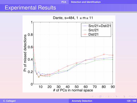
PCA Detection and Identification
Experimental Results
each one of these, and believe that most of these are notanomalies. For example, 2 detections from Abilene and 3detections from Dante appeared to be tra!c from servers toclients on di"erent ports. Another 4 from Dante are smallpoint-to-point flows transferring fewer than 100 small pack-ets, and 5 from Abilene that are frequently recurring Sambaover IP flows that do not appear anomalous. This leaves uswith 4 and 1 true missed detections for Abilene and Danterespectively. The 4 in Abilene belong to two anomalies, aflash crowd and an alpha flow. The 1 in Dante is an alphaflow.
IP-flow Identification. One of Defeat’s advantages is thatit can automatically identify IP flows that were responsiblefor the anomalies in a given time bin. Table 5 shows a small,randomly chosen, set of IP flows that Defeat identified, us-ing the algorithm described in Section 2. In this table, wehave omitted a detailed listing of the anomalous IP flows, forbrevity. We have manually verified these anomalies. UnlikeDefeat, [8] can only automatically identify the time bin dur-ing which an anomaly was detected, and the OD flows con-taining the anomaly or anomalies (a single OD flow mightcontain more than one anomaly, but that method cannotinfer this).
3.1 Exploring the Parameter SpaceDefeat has several parameters which can a"ect its detec-
tion perfomance. We now consider the e"ect of varying theseparameters.
10 20 30 40 50 60 70 80 900
0.2
0.4
0.6
0.8
1
# of PCs in normal space
Pr o
f mis
sed
dete
ctio
ns
Abilene, s=121, 1 ! m ! 11
Src/21+Dst/21Src/21Dst/21
Figure 3: The probability of missed detections asa function of the normal space size for the Abilenedata set.
Normal Space Size. How many principal componentsshould be used to construct the normal subspace? One wayto answer this question is to examine (by plotting graphssimilar to Figure 2) the eigenflows generated by each sketchcorresponding to the principal components (PCs) in order,and determine that component at which the eigenflows startto di"er substantially. We have observed, using this method-ology, that around 10-20 PCs define the normal subspace forboth data sets. Another approach is to examine how De-feat’s performance varies, vis-a-vis [8], with changing num-bers of PCs. Figure 3 and 4 show that across di"erent keydefinitions and for both data sets, Defeat’s missed detectionsare lowest when the normal subspace has 10-20 PCs. For this
10 20 30 40 50 60 70 80 900
0.2
0.4
0.6
0.8
1
# of PCs in normal space
Pr o
f mis
sed
dete
ctio
ns
Dante, s=484, 1 ! m ! 11
Src/21+Dst/21Src/21Dst/21
Figure 4: The probability of missed detections as afunction of the normal space size for the Dante dataset.
reason, we chose 10 PCs in our evaluations; this choice isconsistent with that of [8]. As an aside, notice that misseddetection rates increase dramatically when fewer than 10PCs are used; intuitively, this choice shifts higher volumenormal tra!c into the residual space, making it harder todetect anomalies.
In what follows, we use 10 PCs. Furthermore, we haveomitted, for space reasons, the Abilene data set. However,all our observations below hold for Abilene as well.
Sketch Size. Figure 5 plots Defeat performance as a func-tion of sketch size. Each curve represents a di"erent sketchsize, and di"erent data points represent di"erent votes from11 di"erent hash functions: the point on the top right of acurve represents a detection by at least one hash function(union) and the point on the bottom left represents detec-tions by all hash functions.
Large sketch sizes decrease the missed detection rates andincrease the addtional detection rates. Since, as we showabove, the additional detections are likely to be true anoma-lies, larger sketch sizes perform better than smaller ones.For our data sets, sketch size 1024 is a good choice sincethe probability of detections (1 - missed detection rate) isgreater than 90% for both data sets. Our choice of a sketchsize of 484 in our performance comparison was dictated bythe need to make an even comparison with [8]; however, thisfigure shows that Defeat can perform better (detect moreanomalies, with fewer false alarms) with a larger sketch size.
Number of Hash Functions. How many hash functionsare su!cient for high detection rates? As Figure 6 shows,there exists a knee after which increasing of the number ofhash functions does not improve detection rate. For mostsketch sizes, this knee is the same, at 5 or 6 hash functions.While this needs more extensive data analysis, it is encour-aging to note that a small number of hash functions su!cesfor accurate anomaly detection.
Voting Schemes. Figure 7 plots the detection rates againstthe false alarm rates for di"erent numbers of votes. Thisfigure uses as the definition of true anomalies those foundin our detailed manual inspection, which yields a more ac-curate (and higher) detection probability and (lower) false
C. Callegari Anomaly Detection 129 / 169

PCA Detection and Identification
Experimental Results
Some remarks on the method:The false-positive rate is very sensitive to thedimensionality of the normal subspaceThe effectiveness of PCA is sensitive to the way the trafficmeasurements are aggregatedLarge anomalies can contaminate the normal sub-spacePinpointing the anomalous flows is inherently difficult
C. Callegari Anomaly Detection 130 / 169
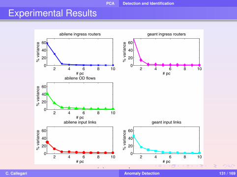
PCA Detection and Identification
Experimental Results
4. TUNABLE PARAMETERSThe following section will evaluate PCA’s sensitivity to
its two key parameters, viz. the number of dimensions thatconstitute its normal subspace in section 4.1 and the detec-tion threshold in section 4.2.
4.1 Size of Normal SubspaceThe number of principal components included in the nor-
mal subspace—the topk parameter—is the most importantparameter to be tuned when using PCA as a tra!c anomalydetector. Past literature has made four important claims inthis context: (i) tra!c traces have low intrinsic dimension-ality, which means that topk can be small, (ii) these first fewprincipal components capture the vast majority of the vari-ance in the data, (iii) the same principal components are alsohighly periodic and thus capture the diurnal trends soughtto be included in the normal subspace, and (iv) identify-ing the separation between normal and anomalous principalcomponents can be done by retaining the first k principalcomponents such that the projection of the tra!c data doesnot contain a 3! deviation from the mean [14, 12]. Thefollowing sub-sections show, in order, that the second claimdoes not hold across all networks and tra!c aggregations,that the e"ectiveness of PCA is very sensitive to the topk
parameter, and that the previously proposed techniques fordetermining topk are inadequate.
4.1.1 Decoupling Size from Captured VarianceEach of our datasets support the previous finding that
tra!c traces have low intrinsic dimensionality, as can beseen from figure 3(a). The figure contains scree plots foreach of the datasets used in our study. A scree plot is aplot of percent variance captured by a given principal com-ponent. We can conclude that tra!c traces have low in-trinsic dimensionality because the corresponding scree plotshave very early knees relative to the original dimensional-ity of the datasets (seen in table 3). This is an importantobservation because it means that only a small fraction ofall principal components need to be included in the normalsubspace to capture the periodic trends that these first fewprincipal components have been shown to exhibit [14].
However, our results do not support the earlier contentionthat the first few principal components necessarily capturethe vast majority of variability in the tra!c matrix, which isdemonstrated by figure 3(b), which is the CDF of 3(a) in log-scale. While the plots in figure 3(a) have knees somewherein the range [2, 6], it is much more di!cult to argue thatsetting topk to a value in this range would correspond toa vast fraction of variance in figure 3(b). For example, ifan Abilene network operator wanted to capture 90% of thevariance for the input-link aggregation, he would need a topk
value that was an order of magnitude larger than previouslyreported in the literature (at least 95). If, on the other hand,he set topk to match up with the knee seen in figure 3(a),he would capture less than half of the total variance.
The purpose of this section is not merely to debunk anearlier coupling of low intrinsic dimensionality and percentvariance captured, but also to highlight that this distinctionis an important one. One should not determine the topk
variable based on percent variance captured (i.e., plot 3(b))because di"erent networks have di"erent natural levels ofvariability, and the normal subspace should capture period-icity as opposed to a certain fraction of variance. For ex-
2 4 6 8 100
20
40
60
abilene input links
# pc
% v
aria
nce
2 4 6 8 100
20
40
60
abilene OD flows
# pc
% v
aria
nce
2 4 6 8 100
20
40
60
abilene ingress routers
# pc
% v
aria
nce
2 4 6 8 100
20
40
60
geant input links
# pc
% v
aria
nce
2 4 6 8 100
20
40
60
geant ingress routers
# pc
% v
aria
nce
(a) scree plots
100
101
102
103
30
40
50
60
70
80
90
100
# principal components
cum
ulat
ive
perc
ent v
aria
nce
capt
ured
abilene input linksabilene OD flowsabilene ingress routersgeant input linksgeant ingress routers
(b) CDF of scree plots
Figure 3: Intrinsic Dimensionality
ample, a research backbone for universities such as Abilenewill likely have a more variable matrix than a tier-1 networkbecause Abilene is (i) smaller, (ii) is used as an experimen-tal network, and (iii) only a very limited set of source hostsgain access to the network. The same heterogeneity is exhib-ited across di"erent tra!c aggregations also, where a morehighly aggregated tra!c aggregation such as ingress routerswill have more stable statistical properties than input links,which may have lots of small flows that are highly variable.It is therefore important to highlight that the topk param-eter should not be determined based on cumulative percentvariance captured.
4.1.2 Sensitivity AnalysisPCA is very sensitive to the topk parameter: We
noted previously that the scree plots for our datasets eachappeared to have knees in the range [2, 6]. While that rangemight appear small, our results indicate that PCA is verysensitive to the number of principal components even withinsuch a limited range. As can be seen from figure 4(a), withinthe [2, 6] range, the false-positive rate for Geant ingress
114
C. Callegari Anomaly Detection 131 / 169

PCA Detection and Identification
Experimental Results
4. TUNABLE PARAMETERSThe following section will evaluate PCA’s sensitivity to
its two key parameters, viz. the number of dimensions thatconstitute its normal subspace in section 4.1 and the detec-tion threshold in section 4.2.
4.1 Size of Normal SubspaceThe number of principal components included in the nor-
mal subspace—the topk parameter—is the most importantparameter to be tuned when using PCA as a tra!c anomalydetector. Past literature has made four important claims inthis context: (i) tra!c traces have low intrinsic dimension-ality, which means that topk can be small, (ii) these first fewprincipal components capture the vast majority of the vari-ance in the data, (iii) the same principal components are alsohighly periodic and thus capture the diurnal trends soughtto be included in the normal subspace, and (iv) identify-ing the separation between normal and anomalous principalcomponents can be done by retaining the first k principalcomponents such that the projection of the tra!c data doesnot contain a 3! deviation from the mean [14, 12]. Thefollowing sub-sections show, in order, that the second claimdoes not hold across all networks and tra!c aggregations,that the e"ectiveness of PCA is very sensitive to the topk
parameter, and that the previously proposed techniques fordetermining topk are inadequate.
4.1.1 Decoupling Size from Captured VarianceEach of our datasets support the previous finding that
tra!c traces have low intrinsic dimensionality, as can beseen from figure 3(a). The figure contains scree plots foreach of the datasets used in our study. A scree plot is aplot of percent variance captured by a given principal com-ponent. We can conclude that tra!c traces have low in-trinsic dimensionality because the corresponding scree plotshave very early knees relative to the original dimensional-ity of the datasets (seen in table 3). This is an importantobservation because it means that only a small fraction ofall principal components need to be included in the normalsubspace to capture the periodic trends that these first fewprincipal components have been shown to exhibit [14].
However, our results do not support the earlier contentionthat the first few principal components necessarily capturethe vast majority of variability in the tra!c matrix, which isdemonstrated by figure 3(b), which is the CDF of 3(a) in log-scale. While the plots in figure 3(a) have knees somewherein the range [2, 6], it is much more di!cult to argue thatsetting topk to a value in this range would correspond toa vast fraction of variance in figure 3(b). For example, ifan Abilene network operator wanted to capture 90% of thevariance for the input-link aggregation, he would need a topk
value that was an order of magnitude larger than previouslyreported in the literature (at least 95). If, on the other hand,he set topk to match up with the knee seen in figure 3(a),he would capture less than half of the total variance.
The purpose of this section is not merely to debunk anearlier coupling of low intrinsic dimensionality and percentvariance captured, but also to highlight that this distinctionis an important one. One should not determine the topk
variable based on percent variance captured (i.e., plot 3(b))because di"erent networks have di"erent natural levels ofvariability, and the normal subspace should capture period-icity as opposed to a certain fraction of variance. For ex-
2 4 6 8 100
20
40
60
abilene input links
# pc
% v
aria
nce
2 4 6 8 100
20
40
60
abilene OD flows
# pc
% v
aria
nce
2 4 6 8 100
20
40
60
abilene ingress routers
# pc
% v
aria
nce
2 4 6 8 100
20
40
60
geant input links
# pc
% v
aria
nce
2 4 6 8 100
20
40
60
geant ingress routers
# pc
% v
aria
nce
(a) scree plots
100
101
102
103
30
40
50
60
70
80
90
100
# principal components
cum
ulat
ive
perc
ent v
aria
nce
capt
ured
abilene input linksabilene OD flowsabilene ingress routersgeant input linksgeant ingress routers
(b) CDF of scree plots
Figure 3: Intrinsic Dimensionality
ample, a research backbone for universities such as Abilenewill likely have a more variable matrix than a tier-1 networkbecause Abilene is (i) smaller, (ii) is used as an experimen-tal network, and (iii) only a very limited set of source hostsgain access to the network. The same heterogeneity is exhib-ited across di"erent tra!c aggregations also, where a morehighly aggregated tra!c aggregation such as ingress routerswill have more stable statistical properties than input links,which may have lots of small flows that are highly variable.It is therefore important to highlight that the topk param-eter should not be determined based on cumulative percentvariance captured.
4.1.2 Sensitivity AnalysisPCA is very sensitive to the topk parameter: We
noted previously that the scree plots for our datasets eachappeared to have knees in the range [2, 6]. While that rangemight appear small, our results indicate that PCA is verysensitive to the number of principal components even withinsuch a limited range. As can be seen from figure 4(a), withinthe [2, 6] range, the false-positive rate for Geant ingress
114
C. Callegari Anomaly Detection 132 / 169

PCA Detection and Identification
Experimental Results
2 3 4 5 6 7 8 9 100
5
10
15
20
25
30
35
# principal components
perc
ent f
alse
pos
itive
sgeant (threshold = 90%)
ingress routersinput links
(a) Geant false-positive rate
2 3 4 5 6 7 8 9 1060
80
100
120
140
160
180
# principal components
tota
l det
ectio
ns
geant (threshold = 90%)
ingress routersinput links
(b) Geant total detections
2 3 4 5 6 7 8 9 1010
20
30
40
50
60
70
# principal components
perc
ent f
alse
pos
itive
s
abilene (threshold = 90%)
ingress routersOD flowsinput links
(c) Abilene false-positive rate
2 3 4 5 6 7 8 9 10200
400
600
800
1000
1200
1400
1600
1800
2000
2200
# principal components
tota
l det
ectio
ns
abilene (threshold = 90%)
ingress routersOD flowsinput links
(d) Abilene total detections
Figure 4: Impact of topk on false-positive rate andtotal detections
routers varies between 3.1% and 15.8%. If one ventures be-yond this range, the performance degradation can be evenmore rapid. In the same figure we can see that the false-positive rate when going from 6 to 8 principal componentsfor Geant input links increases from 9.2% to 31.6%. It istherefore extremely important that the topk parameter becarefully tuned. For the remainder of this paper, we willdefine the ’appropriate’ topk value as the one that we con-sider achieves the best trade-o! between the false-positiverate and the total number of detections.
The appropriate topk value varies across networksand tra!c aggregations: Figure 4 also shows that theappropriate number of principal components to incorporateinto the normal subspace varies across networks and tra"caggregations. For example, the appropriate choice of prin-cipal components is probably 2 for Abilene ingress routers,3 for Geant ingress routers, and 5 for Abilene OD-flows. Itis interesting to note that the relative order of these threedatasets in terms of topk value is identical to their rela-tive ordering in terms of original dimensionality (see: totalnumber of flows in table 3). We hypothesize that this phe-nomenon will hold in general, and further research mightprovide rule-of-thumb guidelines that map!original dimensionality, scree knee" tuples to a topk value.Guidelines are not sound methodology, however, and PCA’ssensitivity to the topk parameter necessitates a robust method-ology.
Comparison of tra!c aggregations: Finally, figure 4shows that the choice of tra"c aggregation has a strongimpact on PCA’s performance. Choosing the right traf-fic aggregation is tricky: too much aggregation will lead tosmooth and predictable flow curves whereas too little aggre-gation yields a very heavy-tailed flow-size distribution (seefigure 2) and hence some highly variable small flows whosespikes are not of interest to network operators. In particular,for both Abilene in figure 4(d) and Geant in figure 4(b), it isclear that the ingress router aggregation consistently detectsfewer anomalies than OD flows and input links. The reasonfor this is that at the level of ingress routers, the data is soaggregated and the flows are so large that most anomaliesare e!ectively drowned. This also means that the anomaliesthat are flagged by PCA when using this aggregation-leveltend to be large and obvious. Hence, at its appropriatetopk value (e.g. 3 for Geant and 2 for Abilene), the ingressrouters aggregation has the lowest false-positive rate of thethree tra"c aggregations studied for both networks.
On the other end of our aggregation spectrum, input links’false-positive rate su!ers as a result of a large fraction ofsmall flows. Abilene input links is particularly bad in fig-ure 4(c) in that its false-positive rate never goes below 40%.It holds across both networks that, at their respective ap-propriate topk values, the input links aggregation has thehighest false-positive rate of the three formalisms. We be-lieve this can be largely contributed to an excess of smallflows whose natural variance cause alarms to be raised bythe PCA tra"c anomaly detector.
For the Abilene network (figures 4(c) and 4(d)), it seemsclear that OD-flows is the tra"c aggregation that achievesthe best overall trade-o! between total detections and false-positive rate. Our findings support earlier papers [14] thathave demonstrated that OD-flows is a fruitful tra"c aggre-gation for detecting network anomalies. For this same rea-son, it is doubly frustrating that we are prevented from try-
115
C. Callegari Anomaly Detection 133 / 169

PCA Detection and Identification
Experimental Results
2 3 4 5 6 7 8 9 100
5
10
15
20
25
30
35
# principal components
perc
ent f
alse
pos
itive
s
geant (threshold = 90%)
ingress routersinput links
(a) Geant false-positive rate
2 3 4 5 6 7 8 9 1060
80
100
120
140
160
180
# principal components
tota
l det
ectio
nsgeant (threshold = 90%)
ingress routersinput links
(b) Geant total detections
2 3 4 5 6 7 8 9 1010
20
30
40
50
60
70
# principal components
perc
ent f
alse
pos
itive
s
abilene (threshold = 90%)
ingress routersOD flowsinput links
(c) Abilene false-positive rate
2 3 4 5 6 7 8 9 10200
400
600
800
1000
1200
1400
1600
1800
2000
2200
# principal components
tota
l det
ectio
ns
abilene (threshold = 90%)
ingress routersOD flowsinput links
(d) Abilene total detections
Figure 4: Impact of topk on false-positive rate andtotal detections
routers varies between 3.1% and 15.8%. If one ventures be-yond this range, the performance degradation can be evenmore rapid. In the same figure we can see that the false-positive rate when going from 6 to 8 principal componentsfor Geant input links increases from 9.2% to 31.6%. It istherefore extremely important that the topk parameter becarefully tuned. For the remainder of this paper, we willdefine the ’appropriate’ topk value as the one that we con-sider achieves the best trade-o! between the false-positiverate and the total number of detections.
The appropriate topk value varies across networksand tra!c aggregations: Figure 4 also shows that theappropriate number of principal components to incorporateinto the normal subspace varies across networks and tra"caggregations. For example, the appropriate choice of prin-cipal components is probably 2 for Abilene ingress routers,3 for Geant ingress routers, and 5 for Abilene OD-flows. Itis interesting to note that the relative order of these threedatasets in terms of topk value is identical to their rela-tive ordering in terms of original dimensionality (see: totalnumber of flows in table 3). We hypothesize that this phe-nomenon will hold in general, and further research mightprovide rule-of-thumb guidelines that map!original dimensionality, scree knee" tuples to a topk value.Guidelines are not sound methodology, however, and PCA’ssensitivity to the topk parameter necessitates a robust method-ology.
Comparison of tra!c aggregations: Finally, figure 4shows that the choice of tra"c aggregation has a strongimpact on PCA’s performance. Choosing the right traf-fic aggregation is tricky: too much aggregation will lead tosmooth and predictable flow curves whereas too little aggre-gation yields a very heavy-tailed flow-size distribution (seefigure 2) and hence some highly variable small flows whosespikes are not of interest to network operators. In particular,for both Abilene in figure 4(d) and Geant in figure 4(b), it isclear that the ingress router aggregation consistently detectsfewer anomalies than OD flows and input links. The reasonfor this is that at the level of ingress routers, the data is soaggregated and the flows are so large that most anomaliesare e!ectively drowned. This also means that the anomaliesthat are flagged by PCA when using this aggregation-leveltend to be large and obvious. Hence, at its appropriatetopk value (e.g. 3 for Geant and 2 for Abilene), the ingressrouters aggregation has the lowest false-positive rate of thethree tra"c aggregations studied for both networks.
On the other end of our aggregation spectrum, input links’false-positive rate su!ers as a result of a large fraction ofsmall flows. Abilene input links is particularly bad in fig-ure 4(c) in that its false-positive rate never goes below 40%.It holds across both networks that, at their respective ap-propriate topk values, the input links aggregation has thehighest false-positive rate of the three formalisms. We be-lieve this can be largely contributed to an excess of smallflows whose natural variance cause alarms to be raised bythe PCA tra"c anomaly detector.
For the Abilene network (figures 4(c) and 4(d)), it seemsclear that OD-flows is the tra"c aggregation that achievesthe best overall trade-o! between total detections and false-positive rate. Our findings support earlier papers [14] thathave demonstrated that OD-flows is a fruitful tra"c aggre-gation for detecting network anomalies. For this same rea-son, it is doubly frustrating that we are prevented from try-
115
C. Callegari Anomaly Detection 134 / 169

PCA Detection and Identification
Experimental Results
2 3 4 5 6 7 8 9 100
5
10
15
20
25
30
35
# principal components
perc
ent f
alse
pos
itive
s
geant (threshold = 90%)
ingress routersinput links
(a) Geant false-positive rate
2 3 4 5 6 7 8 9 1060
80
100
120
140
160
180
# principal components
tota
l det
ectio
ns
geant (threshold = 90%)
ingress routersinput links
(b) Geant total detections
2 3 4 5 6 7 8 9 1010
20
30
40
50
60
70
# principal components
perc
ent f
alse
pos
itive
sabilene (threshold = 90%)
ingress routersOD flowsinput links
(c) Abilene false-positive rate
2 3 4 5 6 7 8 9 10200
400
600
800
1000
1200
1400
1600
1800
2000
2200
# principal components
tota
l det
ectio
ns
abilene (threshold = 90%)
ingress routersOD flowsinput links
(d) Abilene total detections
Figure 4: Impact of topk on false-positive rate andtotal detections
routers varies between 3.1% and 15.8%. If one ventures be-yond this range, the performance degradation can be evenmore rapid. In the same figure we can see that the false-positive rate when going from 6 to 8 principal componentsfor Geant input links increases from 9.2% to 31.6%. It istherefore extremely important that the topk parameter becarefully tuned. For the remainder of this paper, we willdefine the ’appropriate’ topk value as the one that we con-sider achieves the best trade-o! between the false-positiverate and the total number of detections.
The appropriate topk value varies across networksand tra!c aggregations: Figure 4 also shows that theappropriate number of principal components to incorporateinto the normal subspace varies across networks and tra"caggregations. For example, the appropriate choice of prin-cipal components is probably 2 for Abilene ingress routers,3 for Geant ingress routers, and 5 for Abilene OD-flows. Itis interesting to note that the relative order of these threedatasets in terms of topk value is identical to their rela-tive ordering in terms of original dimensionality (see: totalnumber of flows in table 3). We hypothesize that this phe-nomenon will hold in general, and further research mightprovide rule-of-thumb guidelines that map!original dimensionality, scree knee" tuples to a topk value.Guidelines are not sound methodology, however, and PCA’ssensitivity to the topk parameter necessitates a robust method-ology.
Comparison of tra!c aggregations: Finally, figure 4shows that the choice of tra"c aggregation has a strongimpact on PCA’s performance. Choosing the right traf-fic aggregation is tricky: too much aggregation will lead tosmooth and predictable flow curves whereas too little aggre-gation yields a very heavy-tailed flow-size distribution (seefigure 2) and hence some highly variable small flows whosespikes are not of interest to network operators. In particular,for both Abilene in figure 4(d) and Geant in figure 4(b), it isclear that the ingress router aggregation consistently detectsfewer anomalies than OD flows and input links. The reasonfor this is that at the level of ingress routers, the data is soaggregated and the flows are so large that most anomaliesare e!ectively drowned. This also means that the anomaliesthat are flagged by PCA when using this aggregation-leveltend to be large and obvious. Hence, at its appropriatetopk value (e.g. 3 for Geant and 2 for Abilene), the ingressrouters aggregation has the lowest false-positive rate of thethree tra"c aggregations studied for both networks.
On the other end of our aggregation spectrum, input links’false-positive rate su!ers as a result of a large fraction ofsmall flows. Abilene input links is particularly bad in fig-ure 4(c) in that its false-positive rate never goes below 40%.It holds across both networks that, at their respective ap-propriate topk values, the input links aggregation has thehighest false-positive rate of the three formalisms. We be-lieve this can be largely contributed to an excess of smallflows whose natural variance cause alarms to be raised bythe PCA tra"c anomaly detector.
For the Abilene network (figures 4(c) and 4(d)), it seemsclear that OD-flows is the tra"c aggregation that achievesthe best overall trade-o! between total detections and false-positive rate. Our findings support earlier papers [14] thathave demonstrated that OD-flows is a fruitful tra"c aggre-gation for detecting network anomalies. For this same rea-son, it is doubly frustrating that we are prevented from try-
115
C. Callegari Anomaly Detection 135 / 169

PCA Detection and Identification
Experimental Results
2 3 4 5 6 7 8 9 100
5
10
15
20
25
30
35
# principal components
perc
ent f
alse
pos
itive
s
geant (threshold = 90%)
ingress routersinput links
(a) Geant false-positive rate
2 3 4 5 6 7 8 9 1060
80
100
120
140
160
180
# principal components
tota
l det
ectio
ns
geant (threshold = 90%)
ingress routersinput links
(b) Geant total detections
2 3 4 5 6 7 8 9 1010
20
30
40
50
60
70
# principal components
perc
ent f
alse
pos
itive
s
abilene (threshold = 90%)
ingress routersOD flowsinput links
(c) Abilene false-positive rate
2 3 4 5 6 7 8 9 10200
400
600
800
1000
1200
1400
1600
1800
2000
2200
# principal components
tota
l det
ectio
nsabilene (threshold = 90%)
ingress routersOD flowsinput links
(d) Abilene total detections
Figure 4: Impact of topk on false-positive rate andtotal detections
routers varies between 3.1% and 15.8%. If one ventures be-yond this range, the performance degradation can be evenmore rapid. In the same figure we can see that the false-positive rate when going from 6 to 8 principal componentsfor Geant input links increases from 9.2% to 31.6%. It istherefore extremely important that the topk parameter becarefully tuned. For the remainder of this paper, we willdefine the ’appropriate’ topk value as the one that we con-sider achieves the best trade-o! between the false-positiverate and the total number of detections.
The appropriate topk value varies across networksand tra!c aggregations: Figure 4 also shows that theappropriate number of principal components to incorporateinto the normal subspace varies across networks and tra"caggregations. For example, the appropriate choice of prin-cipal components is probably 2 for Abilene ingress routers,3 for Geant ingress routers, and 5 for Abilene OD-flows. Itis interesting to note that the relative order of these threedatasets in terms of topk value is identical to their rela-tive ordering in terms of original dimensionality (see: totalnumber of flows in table 3). We hypothesize that this phe-nomenon will hold in general, and further research mightprovide rule-of-thumb guidelines that map!original dimensionality, scree knee" tuples to a topk value.Guidelines are not sound methodology, however, and PCA’ssensitivity to the topk parameter necessitates a robust method-ology.
Comparison of tra!c aggregations: Finally, figure 4shows that the choice of tra"c aggregation has a strongimpact on PCA’s performance. Choosing the right traf-fic aggregation is tricky: too much aggregation will lead tosmooth and predictable flow curves whereas too little aggre-gation yields a very heavy-tailed flow-size distribution (seefigure 2) and hence some highly variable small flows whosespikes are not of interest to network operators. In particular,for both Abilene in figure 4(d) and Geant in figure 4(b), it isclear that the ingress router aggregation consistently detectsfewer anomalies than OD flows and input links. The reasonfor this is that at the level of ingress routers, the data is soaggregated and the flows are so large that most anomaliesare e!ectively drowned. This also means that the anomaliesthat are flagged by PCA when using this aggregation-leveltend to be large and obvious. Hence, at its appropriatetopk value (e.g. 3 for Geant and 2 for Abilene), the ingressrouters aggregation has the lowest false-positive rate of thethree tra"c aggregations studied for both networks.
On the other end of our aggregation spectrum, input links’false-positive rate su!ers as a result of a large fraction ofsmall flows. Abilene input links is particularly bad in fig-ure 4(c) in that its false-positive rate never goes below 40%.It holds across both networks that, at their respective ap-propriate topk values, the input links aggregation has thehighest false-positive rate of the three formalisms. We be-lieve this can be largely contributed to an excess of smallflows whose natural variance cause alarms to be raised bythe PCA tra"c anomaly detector.
For the Abilene network (figures 4(c) and 4(d)), it seemsclear that OD-flows is the tra"c aggregation that achievesthe best overall trade-o! between total detections and false-positive rate. Our findings support earlier papers [14] thathave demonstrated that OD-flows is a fruitful tra"c aggre-gation for detecting network anomalies. For this same rea-son, it is doubly frustrating that we are prevented from try-
115
C. Callegari Anomaly Detection 136 / 169
PCA Detection and Identification
References
Papagiannaki K. Crovella M. Diot C. Kolaczyk E. D.Lakhina, A. and N. Taft , Structural analysis of networktraffic flows, Tech rep 2004Crovella M. Lakhina, A. and C. Diot , Characterization ofnetwork-wide anomalies in traffic flows, ACMSIGCOMM conference on Internet measurement, 2004Crovella M. Lakhina, A. and C. Diot , Diagnosingnetwork-wide traffic anomalies, Conference onApplications, technologies, architectures, and protocols forcomputer communications, 2004Crovella M. Lakhina, A. and C. Diot , Mining anomaliesusing traffic feature distributions, ACM SIGCOMMComputer Communication Review, 2005Jennifer Rexford Christophe Diot Haakon Ringberg,Augustin Soule , Sensitivity of PCA for Traffic AnomalyDetection, ACM SIGMETRICS, 2007
C. Callegari Anomaly Detection 137 / 169

Wavelet
Outline
1 Introduction
2 Intrusion Detection Expert System
3 Statistical Anomaly Detection
4 Clustering
5 Markovian Models
6 Entropy-based Methods
7 Sketch
8 Principal Component Analysis
9 Wavelet AnalysisCase Study 1
C. Callegari Anomaly Detection 138 / 169

Wavelet
Wavlet Analysis
The wavelets are scaled and translated copies (known as“daughter wavelets”) of a finite-length or fast-decayingoscillating waveform (known as the “mother wavelet”)Wavelet transforms have advantages over traditionalFourier transforms for representing functions that havediscontinuities and sharp peaksThe main difference, with respect to the Fourier transform,is that wavelets are localized in both time and frequencywhereas the standard Fourier transform is only localized infrequency
C. Callegari Anomaly Detection 139 / 169

Wavelet
Wavelet Decomposition
Mother wavelet ψ(t), satisfying the admissibility condition∫|Ψ(ω)|2
|ω|dω < ∞
Wavelet basis
{ψm,n(t)}m,n∈Z ={
a−m/20 ψ
(a−m
0 t − nb0)}
m,n∈Z
Representation of any finite–energy signal x(t) ∈ L2(R) bymeans of its inner products {xm,n}m,n∈Z with the wavelets{ψm,n(t)}m,n∈Z:
xm,n =
∫x(t)·ψm,n(t)dt =
∫x(t)·a−m/2
0 ψ(a−m
0 t − nb0)
dt (8)
Orthonormal dyadic wavelet basisa0 = 2 and b0 = 1Stringent constraints on the mother wavelet
C. Callegari Anomaly Detection 140 / 169
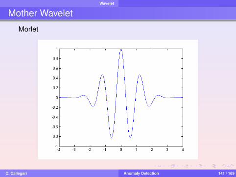
Wavelet
Mother Wavelet
Morlet
C. Callegari Anomaly Detection 141 / 169
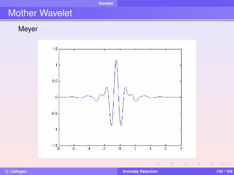
Wavelet
Mother Wavelet
Meyer
C. Callegari Anomaly Detection 142 / 169

Wavelet
Mother Wavelet
Mexican Hat
C. Callegari Anomaly Detection 143 / 169

Wavelet
Filter bank implementation of the Wavelet Transform
Two scale difference equation
ψ(t) =√
2∑
n
gnφ(2t − n) φ(t) =√
2∑
n
hnφ(2t − n)
wheregn = (−1)n−1 h−n−1
Let xxx = (x1, x2, . . .) denote the approximation of a finite–energysignal x(t)
g
h 2
2g
h 2
2g
h 2
2x
Level 1 Level 3Level 2C. Callegari Anomaly Detection 144 / 169

Wavelet
Wavelet and Edge Detection
An edge in an image is a contour across which thebrightness of the image changes abruptlyIn image processing,an edge is often interpreted as oneclass of singularitiesIn a function, singularities can be characterized easily asdiscontinuities where the gradient approaches infinityHowever, image data is discrete, so edges in an imageoften are defined as the local maxima of the gradientWavelet transform has been found to be a remarkable toolto analyze the singularities including the edges and todetect them effectively
C. Callegari Anomaly Detection 145 / 169

Wavelet
Wavelet and Edge Detection
C. Callegari Anomaly Detection 146 / 169

Wavelet
Wavelet and Anomaly Detection
The concept of edge can be easily extended to that ofanomaly in network trafficClassical approaches look at the time series of specifickinds of packets inside aggregate trafficThey detect irregular traffic patterns in traffic trace
Wavelet analysis is applied to evaluate the traffic signal filteredonly at certain scales, and a thresholding technique is used todetect changes
C. Callegari Anomaly Detection 147 / 169

Wavelet Case Study 1
A case study
A Signal Analysis of Network Traffic AnomaliesPaul Barford, Jeffery Kline, David Plonka and Amos RonACM Internet Measurement Workshop 2002The Measurement Data:
SNMP and IP flow datacollected at the border router (Juniper M10) of theUniversity of Wisconsin-Madison campus networkthe campus network consists primarily of four IPv4 class Bnetworks or roughly 256,000 IP addresses of which fewerthan half are utilizedIP connectivity to the commodity Internet and to researchnetworks via about 15 discrete wide-area transit andpeering links all of which terminate into the aforementionedrouter
C. Callegari Anomaly Detection 148 / 169

Wavelet Case Study 1
SNMP Data
The SNMP data was gathered by MRTG at a five minutesampling interval which is commonly used by networkoperatorThe SNMP data consists of the High Capacity interfacestatistics, defined by RFC2863, which were polled usingSNMP version 2cByte and packet counters for each direction of eachwide-area link, specifically these 64-bit counters:ifHCInOctets, ifHCOutOctets, ifHCInUcastPkts, andifHCOutUcastPkt
C. Callegari Anomaly Detection 149 / 169

Wavelet Case Study 1
IP Flow Data
The flow data was gathered using flow-tools and waspost-processed using FlowScanThe Juniper M10 router was running JUNOS 5.0R1.4, andlater JUNOS 5.2R1.4, and was configured to perform“cflowd” flow export with a packet sampling rate of 96This caused 1 of 96 forwarded packets to be sampled, andsubsequently assembled into flow records similar to thosedefined by Cisco’s NetFlow version 5 with similarpacket-sampling-interval and 1 minute flow active-timeoutData were post-processed, so as to store mean value (over5 minutes time-bins) of rate and packet dimension
C. Callegari Anomaly Detection 150 / 169

Wavelet Case Study 1
Anomalies
By manual inspecting the data, 109 anomalies were identified:41 Network Events46 Attacks4 Flash Crowds18 Measurement Events
Necessity of filtering out the daily and weekly variations
C. Callegari Anomaly Detection 151 / 169

Wavelet Case Study 1
The Method
Framelet system, i.e. a redundant wavelet system (whichessentially means that r , the number of high-pass filters, islarger than 1; a simple count shows that, if r > 1, the totalnumber of wavelet coefficients exceeds the length of theoriginal signal)In chosen system, there is one low-pass filter L and threehigh-pass filters H1 , H2 , H3
C. Callegari Anomaly Detection 152 / 169

Wavelet Case Study 1
The analysis platform
Derive from a given signal x (that represents five-minuteaverage measurements over a 2 months period) three outputsignals, as follows
The L(ow frequency)-part of the signal: all thelow-frequency wavelet coefficients from levels 9 and up
should capture patterns and anomalies of very longduration: several days and upsignal here is very sparse (its number of data elements isapproximately 0.4% of those in the original signal), andcaptures weekly patterns in the data quite wellfor many different types of Internet data, the L-part of thesignal reveals a very high degree of regularity andconsistency in the traffic, hence can reliably captureanomalies of long duration
C. Callegari Anomaly Detection 153 / 169

Wavelet Case Study 1
The analysis platform
The M(id frequency)-part of the signal: the waveletscoefficients from frequency levels 6, 7, 8
has zero-meanis supposed to capture mainly the daily variations in thedatadata elements number about 3% of those in the originalsignal
The H(igh frequency)-part of the signal: obtained bythresholding the wavelet coefficients in the first 5 frequencylevels
need for thresholding stems from the fact that most of thedata in the H-part consists of small short-term variations,variations that we think of as “noise”
C. Callegari Anomaly Detection 154 / 169

Wavelet Case Study 1
Detection of anomalies
Normalize the H- and M-parts to have variance oneCompute the local variability of the (normalized) H- andM-parts by computing the variance of the data falling withina moving window of specified sizeThe length of this moving window should depend on theduration of the anomalies that we wish to captured
If we denote the duration of the anomaly by t0 and the timelength of the window for the local deviation by t1, we need,in the ideal situation, to have q = t0/t1 = 1If the quotient q is too small, the anomaly may be blurredand lostIf the quotient is too large, we may be overwhelmed byanomalies that are of very little interest
C. Callegari Anomaly Detection 155 / 169

Wavelet Case Study 1
Detection of anomalies
Combine the local variability of the H- part and M- part ofthe signal using a weighted sum. The result is theV(ariable)-part of the signalApply thresholding to the V-signal. By measuring the peakheight and peak width of the V-signal, one is able to beginto identify anomalies, their duration, and their relativeintensityNeeded Parameters:
M- window sizeH- window sizeweights assigned to the M- and H-partsthreshold
C. Callegari Anomaly Detection 156 / 169

Wavelet Case Study 1
Experimental Results
IN PROCEEDINGS OF ACM SIGCOMM INTERNET MEASUREMENTWORKSHOP 2002 6
sufficient intensity are also detected.2. Combine the local variability of the H-part and M-part of thesignal using a weighted sum. The result is the V(ariable)-part ofthe signal.3. Apply thresholding to the V-signal. By measuring the peakheight and peak width of the V-signal, one is able to begin toidentify anomalies, their duration, and their relative intensity.We provide further details of our application of this technique inSection V.While this approach to identifying anomalies that occur over
periods of hours appears to be promising, it is only the first stepin a process of automated anomaly detection based on the use ofwavelet coefficients. Our choice of using scale dependent win-dowing to calculate deviation score is motivated by simplicity.This approach enabled us to easily quantify the significance oflocal events by using the reconstructed signal’s local variability.In the future, we may find that direct use of combinations ofwavelet and approximation coefficients (or other components)will be sufficient for accurate automated anomaly detection. Tothat end, as future work, we plan to investigate which compo-nents provide the best descrimination and to employ machinelearning tools and techniques to develop more robust automatedanomaly detectors. This approach will enable us to evaluatequantitatively which combinations of wavelet (or other) featuresprovide the best detection capability.
B. The IMAPIT Analysis Environment
The IMAPIT environment we developed for this study hastwo significant components: a data archive and a signal analysisplatform. The data archive uses RRDTOOL (mentioned in Sec-tion III) which provides a flexible database and front-end for ourIP flow and SNMP data. The analysis platform is a framelet sig-nal analysis and visualization system that enables a wide rangeof wavelet systems to be applied to signals.Signal manipulation and data preparation in IMAPIT analysis
was performed using a modified version of the freely-availableLastWave software package [26]. In addition to wavelet decom-position, we implemented our deviation score method for expos-ing signal anomalies. Both flow and SNMP time-series data canbe used as input to compute the deviation score of a signal.Calculating the deviation score has four parameters: an M-
window size, an H-window size, and the weights assigned to theM- and H-parts. We used only a single constant set of parametervalues to produce the results in Section V. However, one cantune IMAPIT’s sensitivity to instantaneous events by modifyingthe movingwindow size used in constructing the local deviation;a smaller window is more sensitive. The weights used on the M-and H-parts allow one to emphasize events of longer or shorterduration.In our analysis, we found most anomalies in our journal had
deviation scores of 2.0 or higher. We consider scores of 2.0 orhigher as “high-confidence”, and those with scores below 1.25as “low-confidence”. Where deviation scores are plotted in fig-ures in Section V, we show the score as a grey band clippedbetween 1.25 and 2.0 on the vertical axis, as labeled on the rightside. An evaluation of deviation scoring as a means for anomalydetection can be found in Section VI.
V. RESULTSWe decompose each signal under analysis into three distinct
signals (low/mid/high). As a point of reference, if the signalunder analysis is 1 week long (the period used to evaluate short-lived anomalies), the H-part is frequency levels 1,2,3; the M-part is frequency levels 4,5; the L-part is the remainder. If thesignal is 8 weeks long (the period used to evaluate long-livedanomalies), the M-part is frequency levels 6,7,8; and the L-partis the remainder.
0 5 M
10 M15 M20 M
Byte
s/sec bytes, original signal
One Autonomous System to Campus, Inbound, 2001-DEC-16 through 2001-DEC-23
-6 M-4 M-2 M
0 2 M4 M6 M
bytes, high-band
-4 M-2 M
0 2 M4 M
bytes, mid-band
Sat Sun Mon Tue Wed Thu Fri Sat Sun0
5 M10 M15 M20 M
bytes, low-band
Fig. 1. Aggregate byte traffi c from IP flow data for a typical week plushigh/mid/low decomposition.
0 5 M
10 M15 M20 M
Byte
s/sec bytes, original signal
One Interface to Campus, Inbound, 2001-DEC-16 through 2001-DEC-23
-6 M-4 M-2 M
0 2 M4 M6 M
bytes, high-band
-4 M-2 M
0 2 M4 M
bytes, mid-band
Sat Sun Mon Tue Wed Thu Fri Sat Sun0
5 M10 M15 M20 M
bytes, low-band
Fig. 2. Aggregate SNMP byte traffi c for the same week as Figure 1 plushigh/mid/low decomposition.
A. Characteristics of Ambient Traffic
It is essential to establish a baseline for traffic free of anoma-lies as a means for calibrating our results. Many studies de-scribe the essential features of network traffic (e.g. [4]) includ-ing the standard daily and weekly cycles. Figure 1 shows thebyte counts of inbound traffic to campus from the commodity
C. Callegari Anomaly Detection 157 / 169

Wavelet Case Study 1
Experimental Results
IN PROCEEDINGS OF ACM SIGCOMM INTERNET MEASUREMENTWORKSHOP 2002 6
sufficient intensity are also detected.2. Combine the local variability of the H-part and M-part of thesignal using a weighted sum. The result is the V(ariable)-part ofthe signal.3. Apply thresholding to the V-signal. By measuring the peakheight and peak width of the V-signal, one is able to begin toidentify anomalies, their duration, and their relative intensity.We provide further details of our application of this technique inSection V.While this approach to identifying anomalies that occur over
periods of hours appears to be promising, it is only the first stepin a process of automated anomaly detection based on the use ofwavelet coefficients. Our choice of using scale dependent win-dowing to calculate deviation score is motivated by simplicity.This approach enabled us to easily quantify the significance oflocal events by using the reconstructed signal’s local variability.In the future, we may find that direct use of combinations ofwavelet and approximation coefficients (or other components)will be sufficient for accurate automated anomaly detection. Tothat end, as future work, we plan to investigate which compo-nents provide the best descrimination and to employ machinelearning tools and techniques to develop more robust automatedanomaly detectors. This approach will enable us to evaluatequantitatively which combinations of wavelet (or other) featuresprovide the best detection capability.
B. The IMAPIT Analysis Environment
The IMAPIT environment we developed for this study hastwo significant components: a data archive and a signal analysisplatform. The data archive uses RRDTOOL (mentioned in Sec-tion III) which provides a flexible database and front-end for ourIP flow and SNMP data. The analysis platform is a framelet sig-nal analysis and visualization system that enables a wide rangeof wavelet systems to be applied to signals.Signal manipulation and data preparation in IMAPIT analysis
was performed using a modified version of the freely-availableLastWave software package [26]. In addition to wavelet decom-position, we implemented our deviation score method for expos-ing signal anomalies. Both flow and SNMP time-series data canbe used as input to compute the deviation score of a signal.Calculating the deviation score has four parameters: an M-
window size, an H-window size, and the weights assigned to theM- and H-parts. We used only a single constant set of parametervalues to produce the results in Section V. However, one cantune IMAPIT’s sensitivity to instantaneous events by modifyingthe movingwindow size used in constructing the local deviation;a smaller window is more sensitive. The weights used on the M-and H-parts allow one to emphasize events of longer or shorterduration.In our analysis, we found most anomalies in our journal had
deviation scores of 2.0 or higher. We consider scores of 2.0 orhigher as “high-confidence”, and those with scores below 1.25as “low-confidence”. Where deviation scores are plotted in fig-ures in Section V, we show the score as a grey band clippedbetween 1.25 and 2.0 on the vertical axis, as labeled on the rightside. An evaluation of deviation scoring as a means for anomalydetection can be found in Section VI.
V. RESULTSWe decompose each signal under analysis into three distinct
signals (low/mid/high). As a point of reference, if the signalunder analysis is 1 week long (the period used to evaluate short-lived anomalies), the H-part is frequency levels 1,2,3; the M-part is frequency levels 4,5; the L-part is the remainder. If thesignal is 8 weeks long (the period used to evaluate long-livedanomalies), the M-part is frequency levels 6,7,8; and the L-partis the remainder.
0 5 M
10 M15 M20 M
Byte
s/sec bytes, original signal
One Autonomous System to Campus, Inbound, 2001-DEC-16 through 2001-DEC-23
-6 M-4 M-2 M
0 2 M4 M6 M
bytes, high-band
-4 M-2 M
0 2 M4 M
bytes, mid-band
Sat Sun Mon Tue Wed Thu Fri Sat Sun0
5 M10 M15 M20 M
bytes, low-band
Fig. 1. Aggregate byte traffi c from IP flow data for a typical week plushigh/mid/low decomposition.
0 5 M
10 M15 M20 M
Byte
s/sec bytes, original signal
One Interface to Campus, Inbound, 2001-DEC-16 through 2001-DEC-23
-6 M-4 M-2 M
0 2 M4 M6 M
bytes, high-band
-4 M-2 M
0 2 M4 M
bytes, mid-band
Sat Sun Mon Tue Wed Thu Fri Sat Sun0
5 M10 M15 M20 M
bytes, low-band
Fig. 2. Aggregate SNMP byte traffi c for the same week as Figure 1 plushigh/mid/low decomposition.
A. Characteristics of Ambient Traffic
It is essential to establish a baseline for traffic free of anoma-lies as a means for calibrating our results. Many studies de-scribe the essential features of network traffic (e.g. [4]) includ-ing the standard daily and weekly cycles. Figure 1 shows thebyte counts of inbound traffic to campus from the commodity
C. Callegari Anomaly Detection 158 / 169

Wavelet Case Study 1
Experimental ResultsIN PROCEEDINGS OF ACM SIGCOMM INTERNET MEASUREMENTWORKSHOP 2002 7
Internet Service Provider during a typical week. The figure alsoshows the wavelet decomposition of the signal into high, mid,and low-band components corresponding to the H-, M-, and L-parts discussed in Section IV. The regular daily component ofthe signal is very clear in the low band4.In Figure 2, we show the byte traffic for the same week at
the same level of aggregation as measured by SNMP. In thiscase traffic was measured by utilizing high-capacity SNMP in-terface octet counters rather than by selecting the specific BGPAutonomous System number from the exported flow records.The decompositions in Figures 1 and 2 are nearly indistinguish-able. The primary difference is slightly more high-frequency“jitter” in the flow-export-based signal5.
B. Characteristics of Flash Crowds
The first step in our analysis of anomalies is to focus on flashcrowd events. Our choice of investigating flash crowds first isdue to their long lived features which should be exposed by themid and low-band filters. This suggests that analysis of eitherSNMP or flow-based data is suitable, however we focus on flow-based data. Figure 3 shows the decomposition of eight weeksof outbound traffic from one of the campus’ class-B networkswhich contains a popular ftp mirror server for Linux releases.During these weeks, two releases of popular Linux distributionsoccurred, resulting in heavy use of the campus mirror server. Inthis and subsequent figures, grey boxes were added by hand tofocus the reader’s attention on the particular anomaly (the posi-tion of each box was determined by simple visual inspection).Attention should again focus on the low-band signal. The low-band signal highlights each event clearly as well as the long-lived aspect of the second event.Another way to consider the effects of flash crowds is from
the perspective of their impact on the typical sizes of packets.The intuition here is that large data/software releases should re-sult in an increase in average packet size for outbound HTTPtraffic and therefore packet size may be an effective means forexposing flash crowds. Figure 4 shows eight weeks of outboundHTTP traffic and highlights another flash crowd anomaly fromour data set. This anomaly was the result of network packettraces being made available on a campus web server. Curiously,for unrelated reasons, the server for this data set had its kernelcustomized to use a TCP Maximum Segment Size of 512. Boththe mid-band and low-band signals in this figure show that theoutbound HTTP packets from this server were, in fact, able toredefine the campus’ average HTTP packet size. It is also inter-esting to note that the packet size signal becomes more stable(the signal has fewer artifacts) during this flash crowd event.This is particularly visible in the mid-band. Since flash crowdstypically involve a single application, it seems likely that thatapplication’s packet size “profile” temporarily dominates.
4We could easily expose the weekly component of the signal using higheraggregation fi lters, however weekly behavior is not important for the groups ofanomalies we consider in this study.
5We will employ formal methods to quantify the difference between SNMPand flow signals and their decompositions in future work.
Oct-01 Oct-08 Oct-15 Oct-22 Oct-29 Nov-05 Nov-12 Nov-19 Nov-260
5 M
10 M
15 M
20 MOutbound Class-B Network Bytes, low-band
-10 M
-5 M
0
5 M Outbound Class-B Network Bytes, mid-band
0 5 M
10 M15 M20 M25 M30 M
Byte
s/sec
Outbound Class-B Network Bytes, original signal
Class-B Network, Outbound, 2001-SEP-30 through 2001-NOV-25
Fig. 3. Baseline signal of byte traffi c for a one week on either side of a flashcrowd anomaly caused by a software release plus high/mid/low decomposi-tion.
Oct-01 Oct-08 Oct-15 Oct-22 Oct-29 Nov-05 Nov-12 Nov-19 Nov-260
500
1000
1500
outbound HTTP average packet size, low-band
-300 -200 -100
0 100 200 300
outound HTTP average packet size, mid-band
0
500
1000
1500
Byte
s
outbound HTTP average packet size signal
Campus HTTP, Outbound, 2001-SEP-30 through 2001-NOV-25
Fig. 4. Baseline signal of average HTTP packet sizes (bytes) for four weeks oneither side of a flash crowd anomaly plus mid/low decomposition.
C. Characteristics of Short-term Anomalies
Short-term anomalies comprise attacks, network outages, andmeasurement anomalies. The coarse-grained (5 minute inter-vals) nature of our measurements complicates discriminationbetween these categories of anomalies, thus we consider themas a group. We evaluated 105 short-term anomalies using dif-ferent combinations of data to determine how best expose theirfeatures (we present analysis of several examples of short-termanomalies to highlight their general features). In contrast to flashcrowds, short-term anomaly features should be best exposed bymid-band and high-band filters which isolate short-timescale as-pects of signals.Figure 5 shows a decomposition of TCP flow counts which
exposes two inbound denial-of-service (DoS) attacks that oc-curred during the same one week period. These two attackswere floods of 40-byte TCP SYN packets destined for the samecampus host. Because the flood packets had dynamic source ad-
C. Callegari Anomaly Detection 159 / 169

Wavelet Case Study 1
Experimental Results
IN PROCEEDINGS OF ACM SIGCOMM INTERNET MEASUREMENTWORKSHOP 2002 7
Internet Service Provider during a typical week. The figure alsoshows the wavelet decomposition of the signal into high, mid,and low-band components corresponding to the H-, M-, and L-parts discussed in Section IV. The regular daily component ofthe signal is very clear in the low band4.In Figure 2, we show the byte traffic for the same week at
the same level of aggregation as measured by SNMP. In thiscase traffic was measured by utilizing high-capacity SNMP in-terface octet counters rather than by selecting the specific BGPAutonomous System number from the exported flow records.The decompositions in Figures 1 and 2 are nearly indistinguish-able. The primary difference is slightly more high-frequency“jitter” in the flow-export-based signal5.
B. Characteristics of Flash Crowds
The first step in our analysis of anomalies is to focus on flashcrowd events. Our choice of investigating flash crowds first isdue to their long lived features which should be exposed by themid and low-band filters. This suggests that analysis of eitherSNMP or flow-based data is suitable, however we focus on flow-based data. Figure 3 shows the decomposition of eight weeksof outbound traffic from one of the campus’ class-B networkswhich contains a popular ftp mirror server for Linux releases.During these weeks, two releases of popular Linux distributionsoccurred, resulting in heavy use of the campus mirror server. Inthis and subsequent figures, grey boxes were added by hand tofocus the reader’s attention on the particular anomaly (the posi-tion of each box was determined by simple visual inspection).Attention should again focus on the low-band signal. The low-band signal highlights each event clearly as well as the long-lived aspect of the second event.Another way to consider the effects of flash crowds is from
the perspective of their impact on the typical sizes of packets.The intuition here is that large data/software releases should re-sult in an increase in average packet size for outbound HTTPtraffic and therefore packet size may be an effective means forexposing flash crowds. Figure 4 shows eight weeks of outboundHTTP traffic and highlights another flash crowd anomaly fromour data set. This anomaly was the result of network packettraces being made available on a campus web server. Curiously,for unrelated reasons, the server for this data set had its kernelcustomized to use a TCP Maximum Segment Size of 512. Boththe mid-band and low-band signals in this figure show that theoutbound HTTP packets from this server were, in fact, able toredefine the campus’ average HTTP packet size. It is also inter-esting to note that the packet size signal becomes more stable(the signal has fewer artifacts) during this flash crowd event.This is particularly visible in the mid-band. Since flash crowdstypically involve a single application, it seems likely that thatapplication’s packet size “profile” temporarily dominates.
4We could easily expose the weekly component of the signal using higheraggregation fi lters, however weekly behavior is not important for the groups ofanomalies we consider in this study.
5We will employ formal methods to quantify the difference between SNMPand flow signals and their decompositions in future work.
Oct-01 Oct-08 Oct-15 Oct-22 Oct-29 Nov-05 Nov-12 Nov-19 Nov-260
5 M
10 M
15 M
20 MOutbound Class-B Network Bytes, low-band
-10 M
-5 M
0
5 M Outbound Class-B Network Bytes, mid-band
0 5 M
10 M15 M20 M25 M30 M
Byte
s/sec
Outbound Class-B Network Bytes, original signal
Class-B Network, Outbound, 2001-SEP-30 through 2001-NOV-25
Fig. 3. Baseline signal of byte traffi c for a one week on either side of a flashcrowd anomaly caused by a software release plus high/mid/low decomposi-tion.
Oct-01 Oct-08 Oct-15 Oct-22 Oct-29 Nov-05 Nov-12 Nov-19 Nov-260
500
1000
1500
outbound HTTP average packet size, low-band
-300 -200 -100
0 100 200 300
outound HTTP average packet size, mid-band
0
500
1000
1500
Byte
s
outbound HTTP average packet size signal
Campus HTTP, Outbound, 2001-SEP-30 through 2001-NOV-25
Fig. 4. Baseline signal of average HTTP packet sizes (bytes) for four weeks oneither side of a flash crowd anomaly plus mid/low decomposition.
C. Characteristics of Short-term Anomalies
Short-term anomalies comprise attacks, network outages, andmeasurement anomalies. The coarse-grained (5 minute inter-vals) nature of our measurements complicates discriminationbetween these categories of anomalies, thus we consider themas a group. We evaluated 105 short-term anomalies using dif-ferent combinations of data to determine how best expose theirfeatures (we present analysis of several examples of short-termanomalies to highlight their general features). In contrast to flashcrowds, short-term anomaly features should be best exposed bymid-band and high-band filters which isolate short-timescale as-pects of signals.Figure 5 shows a decomposition of TCP flow counts which
exposes two inbound denial-of-service (DoS) attacks that oc-curred during the same one week period. These two attackswere floods of 40-byte TCP SYN packets destined for the samecampus host. Because the flood packets had dynamic source ad-
C. Callegari Anomaly Detection 160 / 169

Wavelet Case Study 1
Experimental Results
IN PROCEEDINGS OF ACM SIGCOMM INTERNET MEASUREMENTWORKSHOP 2002 8
dresses and TCP port numbers, the flood was reported as many“degenerate” flows, having only one packet per flow. As pre-dicted, the decomposition easily isolates the anomaly signal inthe high and mid bands. By separating these signals from thelonger time-scale behavior, we have new signals which may beamenable to detection by thresholding.
0 100 200 300 400
Flow
s/se
c Inbound TCP Flows, original signal
Campus TCP, Inbound, 2002-FEB-03 through 2002-FEB-10
0 50
100 150 200
Inbound TCP Flows, high-band
-30 -20 -10
0 10 20 30
Inbound TCP Flows, mid-band
Sun Mon Tue Wed Thu Fri Sat0
100 200 300 400
Inbound TCP Flows, low-band
Fig. 5. Baseline signal of packet flows for a one week period highlighting twoshort-lived DoS attack anomalies plus high/mid/low decomposition.
0
10 M
20 M
30 M
Byt
es/s
ec Inbound TCP Bytes, original signal
Campus TCP, Inbound, 2002-FEB-10 through 2002-FEB-17
-4 M-2 M
0 2 M4 M6 M8 M
Inbound TCP Bytes, high-band
-2 M0
2 M4 M6 M
Inbound TCP Bytes, mid-band
Sun Mon Tue Wed Thu Fri Sat0
10 M
20 M
30 MInbound TCP Bytes, low-band
Fig. 6. Baseline signal of byte traffi c from flow data for a one week period show-ing three short-lived measurement anomalies plus high/mid/low decomposi-tion.
Another type of short-term anomaly is shown in Figure 6.This figure shows a periodic sequence of three measurementanomalies observed over a three day period. This was foundto be a host in the outside world performing nightly backupsto a campus backup server. The large volume of traffic eachday was due to misconfiguration of the client backup software.As in the prior example, the decomposition easily isolates theanomaly signal in the high and mid bands while the low bandis not affected by the anomaly. However if this anomaly hadbeen intended behavior, accounting for it in high and mid bandswould require additional filters in our analysis platform.
D. A Discriminator for Short-term Anomalies
One of the objectives of this work is to provide a basis forautomating anomaly detection. It is important for any anomalydetection mechanism to minimize false positives and false neg-atives. Our analysis led to the development of the “devia-tion score” discrimination function for short-term anomalies de-scribed in Section IV.Figure 7 shows how deviation scores can be used to highlight
a series of short-term anomalies. The figure shows inbound TCPpacket rate during a week plus three anomalies that might other-wise be difficult to discern from the baseline signal. Two of theanomalies are DoS floods that are easily detected and exposedautomatically by their deviation scores and are marked by thefirst and second grey bands. Note, the bands are actually scorevalues as shown by the scale on the right of the figure (the left-most score does not quite reach 2). The third band marks anmeasurement anomaly unrelated to the DoS attacks.
Sun Mon Tue Wed Thu Fri Sat
1.5
2
Scor
e
Deviation Score
Sun Mon Tue Wed Thu Fri Sat0
10 k
20 k
30 k
40 k
50 k
Pack
ets/
sec
Inbound TCP Packets
Campus TCP, Inbound, 2002-FEB-03 through 2002-FEB-10
Fig. 7. Deviation analysis exposing two DoS attacks and one measurementanomaly in for a one week period in packet count data.
In Figure 8, we present a deviation analysis during a weekcontaining a network outage. This outage affected about onefourth of the campus’ IPv4 address space, and therefore causedan overall decrease in traffic. For each traffic measurement met-ric (packets, bytes, flows), inbound or outbound, our deviationscoring identified and marked the anomaly. This suggests thatit is feasible to use a “rules based” approach or weighted aver-age to determine the type or scope of the anomaly based on theaccumulated impact of a set of deviation scores.
E. Exposing Anomalies in Aggregate Signals
An important issue in detecting traffic anomalies is the rela-tionship between the strength of an anomaly’s signal in a set ofaggregated traffic. This is most easily considered with respectto the point at which measurement data is collected in a net-work. Intuition would say that an anomaly measured close to itssource should be very evident while the same anomaly wouldbe less evident if its signal were aggregated with a large amountof other traffic. We investigate this issue by isolating a specificsubnet in which a system is the victim of a DoS attack.Figure 9 shows the deviation analysis of two inbound DoS
floods within the aggregate traffic of the victims 254 host subnet
C. Callegari Anomaly Detection 161 / 169
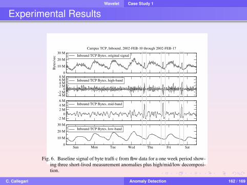
Wavelet Case Study 1
Experimental Results
IN PROCEEDINGS OF ACM SIGCOMM INTERNET MEASUREMENTWORKSHOP 2002 8
dresses and TCP port numbers, the flood was reported as many“degenerate” flows, having only one packet per flow. As pre-dicted, the decomposition easily isolates the anomaly signal inthe high and mid bands. By separating these signals from thelonger time-scale behavior, we have new signals which may beamenable to detection by thresholding.
0 100 200 300 400
Flow
s/se
c Inbound TCP Flows, original signal
Campus TCP, Inbound, 2002-FEB-03 through 2002-FEB-10
0 50
100 150 200
Inbound TCP Flows, high-band
-30 -20 -10
0 10 20 30
Inbound TCP Flows, mid-band
Sun Mon Tue Wed Thu Fri Sat0
100 200 300 400
Inbound TCP Flows, low-band
Fig. 5. Baseline signal of packet flows for a one week period highlighting twoshort-lived DoS attack anomalies plus high/mid/low decomposition.
0
10 M
20 M
30 MB
ytes
/sec Inbound TCP Bytes, original signal
Campus TCP, Inbound, 2002-FEB-10 through 2002-FEB-17
-4 M-2 M
0 2 M4 M6 M8 M
Inbound TCP Bytes, high-band
-2 M0
2 M4 M6 M
Inbound TCP Bytes, mid-band
Sun Mon Tue Wed Thu Fri Sat0
10 M
20 M
30 MInbound TCP Bytes, low-band
Fig. 6. Baseline signal of byte traffi c from flow data for a one week period show-ing three short-lived measurement anomalies plus high/mid/low decomposi-tion.
Another type of short-term anomaly is shown in Figure 6.This figure shows a periodic sequence of three measurementanomalies observed over a three day period. This was foundto be a host in the outside world performing nightly backupsto a campus backup server. The large volume of traffic eachday was due to misconfiguration of the client backup software.As in the prior example, the decomposition easily isolates theanomaly signal in the high and mid bands while the low bandis not affected by the anomaly. However if this anomaly hadbeen intended behavior, accounting for it in high and mid bandswould require additional filters in our analysis platform.
D. A Discriminator for Short-term Anomalies
One of the objectives of this work is to provide a basis forautomating anomaly detection. It is important for any anomalydetection mechanism to minimize false positives and false neg-atives. Our analysis led to the development of the “devia-tion score” discrimination function for short-term anomalies de-scribed in Section IV.Figure 7 shows how deviation scores can be used to highlight
a series of short-term anomalies. The figure shows inbound TCPpacket rate during a week plus three anomalies that might other-wise be difficult to discern from the baseline signal. Two of theanomalies are DoS floods that are easily detected and exposedautomatically by their deviation scores and are marked by thefirst and second grey bands. Note, the bands are actually scorevalues as shown by the scale on the right of the figure (the left-most score does not quite reach 2). The third band marks anmeasurement anomaly unrelated to the DoS attacks.
Sun Mon Tue Wed Thu Fri Sat
1.5
2
Scor
e
Deviation Score
Sun Mon Tue Wed Thu Fri Sat0
10 k
20 k
30 k
40 k
50 k
Pack
ets/
sec
Inbound TCP Packets
Campus TCP, Inbound, 2002-FEB-03 through 2002-FEB-10
Fig. 7. Deviation analysis exposing two DoS attacks and one measurementanomaly in for a one week period in packet count data.
In Figure 8, we present a deviation analysis during a weekcontaining a network outage. This outage affected about onefourth of the campus’ IPv4 address space, and therefore causedan overall decrease in traffic. For each traffic measurement met-ric (packets, bytes, flows), inbound or outbound, our deviationscoring identified and marked the anomaly. This suggests thatit is feasible to use a “rules based” approach or weighted aver-age to determine the type or scope of the anomaly based on theaccumulated impact of a set of deviation scores.
E. Exposing Anomalies in Aggregate Signals
An important issue in detecting traffic anomalies is the rela-tionship between the strength of an anomaly’s signal in a set ofaggregated traffic. This is most easily considered with respectto the point at which measurement data is collected in a net-work. Intuition would say that an anomaly measured close to itssource should be very evident while the same anomaly wouldbe less evident if its signal were aggregated with a large amountof other traffic. We investigate this issue by isolating a specificsubnet in which a system is the victim of a DoS attack.Figure 9 shows the deviation analysis of two inbound DoS
floods within the aggregate traffic of the victims 254 host subnet
C. Callegari Anomaly Detection 162 / 169

Wavelet Case Study 1
Experimental Results
IN PROCEEDINGS OF ACM SIGCOMM INTERNET MEASUREMENTWORKSHOP 2002 8
dresses and TCP port numbers, the flood was reported as many“degenerate” flows, having only one packet per flow. As pre-dicted, the decomposition easily isolates the anomaly signal inthe high and mid bands. By separating these signals from thelonger time-scale behavior, we have new signals which may beamenable to detection by thresholding.
0 100 200 300 400
Flow
s/se
c Inbound TCP Flows, original signal
Campus TCP, Inbound, 2002-FEB-03 through 2002-FEB-10
0 50
100 150 200
Inbound TCP Flows, high-band
-30 -20 -10
0 10 20 30
Inbound TCP Flows, mid-band
Sun Mon Tue Wed Thu Fri Sat0
100 200 300 400
Inbound TCP Flows, low-band
Fig. 5. Baseline signal of packet flows for a one week period highlighting twoshort-lived DoS attack anomalies plus high/mid/low decomposition.
0
10 M
20 M
30 M
Byt
es/s
ec Inbound TCP Bytes, original signal
Campus TCP, Inbound, 2002-FEB-10 through 2002-FEB-17
-4 M-2 M
0 2 M4 M6 M8 M
Inbound TCP Bytes, high-band
-2 M0
2 M4 M6 M
Inbound TCP Bytes, mid-band
Sun Mon Tue Wed Thu Fri Sat0
10 M
20 M
30 MInbound TCP Bytes, low-band
Fig. 6. Baseline signal of byte traffi c from flow data for a one week period show-ing three short-lived measurement anomalies plus high/mid/low decomposi-tion.
Another type of short-term anomaly is shown in Figure 6.This figure shows a periodic sequence of three measurementanomalies observed over a three day period. This was foundto be a host in the outside world performing nightly backupsto a campus backup server. The large volume of traffic eachday was due to misconfiguration of the client backup software.As in the prior example, the decomposition easily isolates theanomaly signal in the high and mid bands while the low bandis not affected by the anomaly. However if this anomaly hadbeen intended behavior, accounting for it in high and mid bandswould require additional filters in our analysis platform.
D. A Discriminator for Short-term Anomalies
One of the objectives of this work is to provide a basis forautomating anomaly detection. It is important for any anomalydetection mechanism to minimize false positives and false neg-atives. Our analysis led to the development of the “devia-tion score” discrimination function for short-term anomalies de-scribed in Section IV.Figure 7 shows how deviation scores can be used to highlight
a series of short-term anomalies. The figure shows inbound TCPpacket rate during a week plus three anomalies that might other-wise be difficult to discern from the baseline signal. Two of theanomalies are DoS floods that are easily detected and exposedautomatically by their deviation scores and are marked by thefirst and second grey bands. Note, the bands are actually scorevalues as shown by the scale on the right of the figure (the left-most score does not quite reach 2). The third band marks anmeasurement anomaly unrelated to the DoS attacks.
Sun Mon Tue Wed Thu Fri Sat
1.5
2
Scor
e
Deviation Score
Sun Mon Tue Wed Thu Fri Sat0
10 k
20 k
30 k
40 k
50 kPa
cket
s/se
cInbound TCP Packets
Campus TCP, Inbound, 2002-FEB-03 through 2002-FEB-10
Fig. 7. Deviation analysis exposing two DoS attacks and one measurementanomaly in for a one week period in packet count data.
In Figure 8, we present a deviation analysis during a weekcontaining a network outage. This outage affected about onefourth of the campus’ IPv4 address space, and therefore causedan overall decrease in traffic. For each traffic measurement met-ric (packets, bytes, flows), inbound or outbound, our deviationscoring identified and marked the anomaly. This suggests thatit is feasible to use a “rules based” approach or weighted aver-age to determine the type or scope of the anomaly based on theaccumulated impact of a set of deviation scores.
E. Exposing Anomalies in Aggregate Signals
An important issue in detecting traffic anomalies is the rela-tionship between the strength of an anomaly’s signal in a set ofaggregated traffic. This is most easily considered with respectto the point at which measurement data is collected in a net-work. Intuition would say that an anomaly measured close to itssource should be very evident while the same anomaly wouldbe less evident if its signal were aggregated with a large amountof other traffic. We investigate this issue by isolating a specificsubnet in which a system is the victim of a DoS attack.Figure 9 shows the deviation analysis of two inbound DoS
floods within the aggregate traffic of the victims 254 host subnet
C. Callegari Anomaly Detection 163 / 169

Wavelet Case Study 1
Experimental Results
IN PROCEEDINGS OF ACM SIGCOMM INTERNET MEASUREMENTWORKSHOP 2002 9
Inbound
1.5
2
Scor
e
Outbound
1.5
2
Scor
e
Sun Mon Tue Wed Thu Fri Sat
1.5
2
Scor
e
0
10 M
20 M
30 M
Byte
s/sec
0
10 k
20 k
30 k
40 k
Pkts/
sec
Sun Mon Tue Wed Thu Fri Sat0
50
100
150
200
Flow
s/sec
Fig. 8. Deviation analysis exposing a network outage of one (of four) Class-B networks.
Inbound
1.5
2
Scor
e
Outbound
1.5
2
Scor
e
1.5
2
Scor
e
0 100 k200 k300 k400 k500 k600 k
Byte
s/sec
0
5 k
10 k
15 k
20 k
Pkts/
sec
Sun Mon Tue Wed Thu Fri Sat0
50
100
150
200
Flow
s/sec
Sun Mon Tue Wed Thu Fri Sat
Inbound
1.5
2
Scor
e
Outbound
1.5
2
Scor
e
1.5
2
Scor
e
0
10 M
20 M
30 M
Byte
s/sec
0 10 k20 k30 k40 k50 k
Pkts/
sec
Sun Mon Tue Wed Thu Fri Sat0
50100150200250300
Flow
s/sec
Sun Mon Tue Wed Thu Fri Sat
Fig. 9. Deviation analysis of two DoS events as seen in the 254 host subnet containing the victim of the attack (top) and in the aggregate traffi c of the entire campus.
C. Callegari Anomaly Detection 164 / 169

Wavelet Case Study 1
Experimental Results
IN PROCEEDINGS OF ACM SIGCOMM INTERNET MEASUREMENTWORKSHOP 2002 9
Inbound
1.5
2
Scor
e
Outbound
1.5
2
Scor
e
Sun Mon Tue Wed Thu Fri Sat
1.5
2
Scor
e
0
10 M
20 M
30 M
Byte
s/sec
0
10 k
20 k
30 k
40 k
Pkts/
sec
Sun Mon Tue Wed Thu Fri Sat0
50
100
150
200
Flow
s/sec
Fig. 8. Deviation analysis exposing a network outage of one (of four) Class-B networks.
Inbound
1.5
2
Scor
e
Outbound
1.5
2
Scor
e
1.5
2
Scor
e
0 100 k200 k300 k400 k500 k600 k
Byte
s/sec
0
5 k
10 k
15 k
20 k
Pkts/
sec
Sun Mon Tue Wed Thu Fri Sat0
50
100
150
200
Flow
s/sec
Sun Mon Tue Wed Thu Fri Sat
Inbound
1.5
2
Scor
e
Outbound
1.5
2
Scor
e
1.5
2
Scor
e
0
10 M
20 M
30 M
Byte
s/sec
0 10 k20 k30 k40 k50 k
Pkts/
sec
Sun Mon Tue Wed Thu Fri Sat0
50100150200250300
Flow
s/sec
Sun Mon Tue Wed Thu Fri Sat
Fig. 9. Deviation analysis of two DoS events as seen in the 254 host subnet containing the victim of the attack (top) and in the aggregate traffi c of the entire campus.
C. Callegari Anomaly Detection 165 / 169
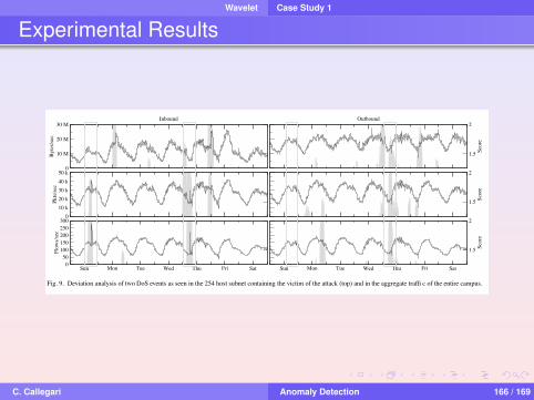
Wavelet Case Study 1
Experimental Results
IN PROCEEDINGS OF ACM SIGCOMM INTERNET MEASUREMENTWORKSHOP 2002 9
Inbound
1.5
2
Scor
e
Outbound
1.5
2
Scor
e
Sun Mon Tue Wed Thu Fri Sat
1.5
2
Scor
e
0
10 M
20 M
30 M
Byte
s/sec
0
10 k
20 k
30 k
40 k
Pkts/
sec
Sun Mon Tue Wed Thu Fri Sat0
50
100
150
200
Flow
s/sec
Fig. 8. Deviation analysis exposing a network outage of one (of four) Class-B networks.
Inbound
1.5
2
Scor
e
Outbound
1.5
2
Scor
e
1.5
2
Scor
e
0 100 k200 k300 k400 k500 k600 k
Byte
s/sec
0
5 k
10 k
15 k
20 k
Pkts/
sec
Sun Mon Tue Wed Thu Fri Sat0
50
100
150
200
Flow
s/sec
Sun Mon Tue Wed Thu Fri Sat
Inbound
1.5
2
Scor
e
Outbound
1.5
2
Scor
e
1.5
2
Scor
e
0
10 M
20 M
30 M
Byte
s/sec
0 10 k20 k30 k40 k50 k
Pkts/
sec
Sun Mon Tue Wed Thu Fri Sat0
50100150200250300
Flow
s/sec
Sun Mon Tue Wed Thu Fri Sat
Fig. 9. Deviation analysis of two DoS events as seen in the 254 host subnet containing the victim of the attack (top) and in the aggregate traffi c of the entire campus.
C. Callegari Anomaly Detection 166 / 169
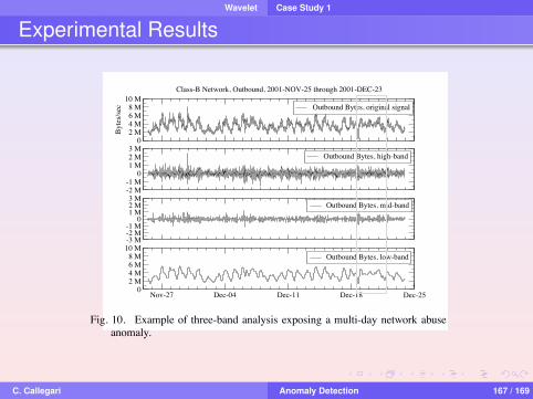
Wavelet Case Study 1
Experimental Results
IN PROCEEDINGS OF ACM SIGCOMM INTERNET MEASUREMENTWORKSHOP 2002 10
and the aggregate traffic of the campus’ four Class-B networks.The top set of graphs in this figure show that deviation scoreseasily highlight the extreme nature of DoS floods in inboundtraffic within the subnet, and that they even highlight the muchless evident outbound traffic anomaly. The bottom set of graphsshow again that deviation scores highlight the same anomalies(as well as a number of others).
F. Hidden Anomalies
Through the application of our methods, we were able to iden-tify a number of “hidden” anomalies in our data sets. These areanomalies that had not been previously identified by the cam-pus network engineers. The majority of these were DoS attacksmost of which could be identified by careful visual inspection.One hidden anomaly of interest is shown in Figure 10. This
figure shows outbound traffic from one of the campus’ class-B networks during a four week period. The duration of thisanomaly prevented its detection via deviation score. Decom-position enabled us to identify an anomaly that had previouslygone unnoticed and was not easily seen visually. The anomalyis most visible following December 18th in the low-band graphwhere traffic remained uncharacteristically high across two sub-sequent days. Follow-up investigation using our repository offlow records showed this anomaly to have been due to of net-work abuse in which four campus hosts had their security com-promised and were being remotely operated as peer-to-peer fileservers.
0 2 M4 M6 M8 M
10 M
Byte
s/sec Outbound Bytes, original signal
Class-B Network, Outbound, 2001-NOV-25 through 2001-DEC-23
-2 M-1 M
0 1 M2 M3 M
Outbound Bytes, high-band
-3 M-2 M-1 M
0 1 M2 M3 M
Outbound Bytes, mid-band
Nov-27 Dec-04 Dec-11 Dec-18 Dec-250
2 M4 M6 M8 M
10 MOutbound Bytes, low-band
Fig. 10. Example of three-band analysis exposing a multi-day network abuseanomaly.
VI. DEVIATION SCORE EVALUATIONWe evaluated the results of our deviation scoring method of
anomaly detection in two ways. First, we selected a set ofanomalies logged in the network operator journal as a baselineand evaluated deviation score detection capability. Secondly, weused the same baseline set of anomalies to evaluate the effective-ness of an alternative detection technique based on Holt-WintersForecasting [12] as a comparison to deviation scoring. We werelimited in the extent to which we could evaluate either detectionmethod since the baseline set of anomalies used in this analy-sis is unlikely to be complete. Therefore, we did not attempt todetermine which method reported more false-positives.
TABLE IICOMPARISON OF ANOMALY DETECTION METHODS.
Total Candidate Candidates detected Candidates detectedAnomalies Evaluated by Deviation Score by Holt-Winters
39 38 37
In each case we were somewhat tolerant of discrepancies be-tween the anomaly timestamps in the journal’s log entries andthe times at which the automated methods reported anomalousnetwork traffic. Specifically, we allowed a discrepancy of asmuch as 1.5 hours since both automated techniques sometimesshift the report significantly from the time of the event’s on-set. The respective identification of anomalies from our evalu-ation set is summarized in Table II. As can be seen, both tech-niques performed well in that their false-negative reports for the39 anomalies in the candidate set were very low.
A. Deviation Score vs. Logged Anomalies
We selected 39 events from the network operator’s log ofanomalies. This subset of events were those for which a suitableamount of evidence had been gathered to label them as “highconfidence” anomalies. This evidence gathering was a tediouseffort often involving the examination of individual flow recordsto identify the specific IP header values for the packets that com-prised the anomaly.Of those 39 anomalies selected as a baseline for evaluation,
deviation score analysis detected 38 of them with a significantlyconfident score of 1.7 or higher. For the single anomaly whichwasn’t detected by our method, its deviation score was substan-tial but less than 1.7. Visual inspection of the plot of this signalshowed that this was due to a more prominent anomaly whichwas detected earlier in the week, which suppressed the magni-tude of the undetected anomaly’s score. This is a side-effect ofthe normalization within the context of the week-long windowwe used in our analysis method.
B. Holt-Winters Forecasting vs. Logged Anomalies
To further evaluate the deviation score, we compared itsanomaly detection results with the Holt-Winters Forecasting andreporting technique that has been implemented in the freely-available development source code of RRDTOOL version 1.1.Holt-Winters Forecasting is a algorithm that builds upon expo-nential smoothing which is described in [27]. The specific im-plementation of Holt-Winters Forecasting is described in [12].We selected this Holt-Winters method for comparison be-
cause it is perhaps the most sophisticated technique that is be-ing used currently by network operators (although not yet bymany!). The most common techniques in use employ simplesite-specific rules-based thresholding. We summarily rejectedthose simple techniques because their rules and magic numbersfor thresholding are often not portable beyond the local networkand because of their general inability to handle seasonal effectssuch as daily cycles in signal amplitude. Both deviation scoreand Holt-Winters analysis can be configured to take a seasonalperiod into consideration, and both are being proposed as possi-ble alternatives to analysis by visual inspection of network traf-
C. Callegari Anomaly Detection 167 / 169
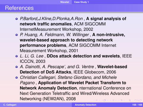
Wavelet Case Study 1
References
P.Barford,J.Kline,D.Plonka,A.Ron , A signal analysis ofnetwork traffic anomalies, ACM SIGCOMMInternetMeasurement Workshop, 2002P. Huang, A. Feldmann, W. Willinger , A non-intrusive,wavelet-based approach to detecting networkperformance problems, ACM SIGCOMM InternetMeasurement Workshop, 2001L. Li, G. Lee , DDos attack detection and wavelets, IEEEICCCN, 2003A. Dainotti, A. Pescape’, and G. Ventre , Wavelet-basedDetection of DoS Attacks, IEEE Globecom, 2006Christian Callegari, Stefano Giordano, and MichelePagano , Application of Wavelet Packet Transform toNetwork Anomaly Detection, nternational Conference onNext Generation Teletraffic and Wired/Wireless AdvancedNetworking (NEW2AN), 2008
C. Callegari Anomaly Detection 168 / 169

Wavelet Case Study 1
Thank You for your attention
C. Callegari Anomaly Detection 169 / 169