Video Anomaly Detection Based on Local Statistical Aggregates ∗

Venkatesh Saligrama Zhu ChenDepartment of Electrical and Computer Engineering

Boston University, Boston, MA 02215srv,zchen@bu.edu

Abstract

Anomalies in many video surveillance applications havelocal spatio-temporal signatures, namely, they occur overa small time window or a small spatial region. The dis-tinguishing feature of these scenarios is that outside thisspatio-temporal anomalous region, activities appear nor-mal. We develop a probabilistic framework to account forsuch local spatio-temporal anomalies. We show that ourframework admits elegant characterization of optimal deci-sion rules.

A key insight of the paper is that if anomalies are lo-cal optimal decision rules are local even when the nomi-nal behavior exhibits global spatial and temporal statisti-cal dependencies. This insight helps collapse the large am-bient data dimension for detecting local anomalies. Con-sequently, consistent data-driven local empirical rules withprovable performance can be derived with limited trainingdata. Our empirical rules are based on scores functions de-rived from local nearest neighbor distances. These rules ag-gregate statistics across spatio-temporal locations & scales,and produce a single composite score for video segments.We demonstrate the efficacy of our scheme on several videosurveillance datasets and compare with existing work.

1. Introduction

Video surveillance has been an area of significant interestin both academia and industry. Recently, anomaly detectionfor video surveillance has gained importance [2, 7, 15, 8, 5,14, 9, 11, 3, 21, 13, 16]. Our focus is on problems, where weare given a set of nominal training videos samples. Basedon these samples we need to determine whether or not a testvideo contains an anomaly. We consider anomalies in mo-tion attributes. Such outliers can include (un)usual motionpatterns of (un)usual objects in (un)usual locations. These

∗Research supported by ONR grant N000141010477, NGA grantHM1582-09-1-0037, NSF grant CCF-0905541, and DHS grant 2008-ST-061- ED0001

encompass anomalies such as dropped baggage, illegal U-turns, and sudden movements.

We focus on anomalies that have local spatio-temporalsignatures. By locality we mean that the spatio-temporalregion surrounding the anomalous region appears to followthe nominal activity and carries little information about theanomaly itself. For instance, the appearance of a bicyclistas shown in Fig. 1 illustrates spatio-temporal locality. Asis seen outside a small window in time or in space the op-tical flow magnitudes look remarkably similar to nominalactivity. We also consider other cases where locality is onlytemporal. These include cases such as sudden crowd move-ment [1] or illegal U-turns [5].

0 50 100 150 200

Frames

60 120 180

Pixel Blocks

(Horizontal Axis)

Figure 1. Illustration of local anomaly. Top: Illustrates frame of avideo segment [15] with anomaly (bicycle). Bottom Panel (Left):Optical flow magnitude averaged over the red block vs. framenumber for nominal and anomalous video segments. (Right): Op-tical flow magnitude averaged over different blocks along horizon-tal pixel blocks for different nominal and anomalous video. Themagnitude outside “anomalous region” looks similar to nominal inboth space and time.

We exploit these ideas by building on recent statisti-

1

cal non-parametric notion of locality [18] and derive data-driven rules for video anomaly detection with predictableperformance and statistical guarantees. Our approach is re-lated to a number of other non-parametric data-driven ap-proaches such as [19, 23] with key differences. Existingstatistical approaches do not account for local anomalies,i.e., anomalies that are localized to a small time intervaland/or spatial region. Our statistical locality notion leads toan elegant characterization of anomaly detection and sug-gests novel empirical rules. A fundamental insight gainedfrom theoretical results is that the optimal decision rules forlocal anomalies are local irrespective of the global statisti-cal dependencies exhibited in the nominal behavior. Thisinsight helps collapse the large ambient data dimension fordetecting local anomalies. Consequently, consistent data-driven local empirical rules with provable performance canbe derived with limited training data. Our local empiricalrules fuse local statistics and produce a composite score fora video segment. Anomalies are declared by ranking com-posite scores for video segments.

The paper is organized as follows. In Sec. 2 we presentoverview of our work and describe related work in videoanomaly detection. In Sec. 3 we present our locality modelstructure to account for local spatio-temporal anomalies.Sec. 4 describes the Neyman-Pearson characterization andderives composite scoring schemes that lead to guaranteeson false alarm control. Sec. 5 presents empirical rules thatapproximate the theoretical composite scores. Proofs of allstatements appear in the supplementary section. Sec. 6presents simulations on benchmark video datasets as wellas comparisons to existing work.

2. Overview and Related WorkOur anomaly detection algorithm is described in Fig. 2.

Our setup extracts local low-level motion descriptors andresembles other common approaches. Adam et al.[2] usehistograms of optical flows at specific “local monitors” toderive decision rules for anomaly detection at those loca-tions. Itti and Baldi consider low-level feature descriptorsat every location [10] and use possion statistics for model-ing nominal activity.

We propose a joint probability distribution of the low-level motion descriptors under nominal as well as anoma-lous distributions. Such joint distributions have also beenconsidered extensively. Kim et al. [13] also extract local op-tical flow and enforce consistency across locations throughMarkov Random Field models. Benezeth et al. [5] usebinary background subtraction to extract motion labels andthen model these local features using a 3D Markov RandomField (MRF). Kratz et al. [14] extract spatio-temporal gra-dient to fit Gaussian model, and then use HMM to detectabnormal events. Mahadevan et al. [15] model the normalcrowd behavior by mixtures of dynamic textures.

Local

KNN

Composite

Scalar Score

Ranking

Scheme

Local

KNN

Test

Video

Training

Video 1

Local

KNN

Training

Video N

Anomaly

Nominal

Local

Feature

Descriptor

Local

Feature

Descriptor

Local

Feature

Descriptor

Spatial

Temporal

Filter

Spatial

Temporal

Filter

Spatial

Temporal

Filter

Weighted

Sum/Max

Weighted

Sum/Max

Weighted

Sum/Max

Figure 2. Overview of Anomaly Detection Algorithm. Motiondescriptors are first extracted and quantized into small blocks.Spatio-Temporal filters at different scales are applied to obtainsmooth estimates at each spatio-temporal location for each featuredescriptor. Local KNN distance for each location is computed fortraining and test video. These local KNN distances are aggregatedto produce a composite score for the test and training video. Thecomposite scores are ranked to determine anomalies.

We introduce novel structural assumptions on the jointdistributions to account for spatial and temporal locality ofanomalies. Our locality assumption leads us to considerstatistics on local 3D brick patches (space-time blocks)across different overlapping locations. These statisticsare obtained through spatio-temporal filters as shown inFig. 2. Our 3D modeling superficially resembles Boimanand Irani [7] but is different. They consider ensembles of3D bricks and derive Gaussian models for matching test en-sembles at a specific location with corresponding ensemblesin a database. However, our goal is statistical and does notattempt to match 3D bricks at a location. Rather (see Fig. 2)we first compute location specific K-nearest neighbor (NN)distance for each 3D brick. We then normalize and com-pute a composite score by aggregating weighted K-NN dis-tances from all the locations. This composite score is rankedagainst other such composite scores associated with train-ing video segments. We then declare low scores as anoma-lies. It turns out that fusing local 3D brick statistics in thismanner has theoretical significance. The empirical compos-ite scoring and ranking scheme asymptotically converges tothe optimal decision rule for maximizing detection powersubject to false alarm constraints.

Our work is also related to Cong et. al. [8] who con-sider dictionary learning methods. There 3D patches withspecific temporal and spatial scale are chosen to match eachscenario. A dictionary of representative patterns are learntbased on training video. Anomalies are declared if the testsample cannot be represented using a sparse set of dictio-nary patterns. It is worth mentioning that we could incorpo-rate their ideas into our scheme. Sparse decomposition foreach spatio-temporal scale can be viewed as a feature vectorthat feeds into our local KNN block (see Fig. 2).

3. Spatio-Temporal Locality Model

We first describe an abstract problem and specialize it tovideo setting in Sec. 3.1. Consider a collection of randomvectors, x = (xv)v∈V , indexed on a graph G = (V,E).The set V is endowed with the usual graph metric d(u, v)defined for any two nodes v and u.

We assume that baseline data x = (xv)v∈V is drawnfrom the null hypothesis H0:

H0 : x ∼ f0(x) (1)

We describe the anomalous distribution as a mixture of lo-cation and scale specific anomalous likelihood models. Forsimplicity of exposition we only consider location specificmixtures at a fixed scale s. Nevertheless, the techniques de-veloped here can be generalized to mixtures across scales1.To this end, let fv(x), Pv be the likelihood function andprior probability associated with location v at scale s. Then,

H1 : x ∼∑v∈V

Pvfv(x) (2)

We next introduce notation to describe our local model. Letωv,s be a ball of radius s around v:

ωv , ωv,s = u | d(u, v) ≤ s

With abuse of notation ωv will generally refer to a ball of afixed radius s at node v. We also denote by ωv,ϵ as the setthat includes all points within an ϵ radius of ωv, i.e.,

ωv,ϵ = u ∈ V | d(u, v) ≤ ϵ, v ∈ ωv

The marginal distribution of f0, fv on a subset ω ⊂ V isdenoted as f0(xω).

Definition 1. We say an anomaly is of local structure if thedistributions f0 and fv satisfy the following Markovian andMask assumptions.(1) Markov Assumption: We say f0 and fv’s satisfy theMarkov assumption if the observation x forms a Markovrandom field. Specifically we assume that there is an ϵ-neighborhood such that xv, v ∈ ωv is conditionally inde-pendent of xu, u ∈ ωv,ϵ when conditioned on the annulusωv,ϵ ∩ ωcv .(2) Mask Assumption: The marginal distribution of f0 andfv on ωcv is identical:

f0(xωcv) = fv(xωc

v)

1H1 : x ∼∑

s

∑v∈V Pv,sfv,s(x) where Pv,s, fv,s(x) are likeli-

hood function and prior probability at location v and scale s.

space

time

anomalous region

fv,s = f0

fv,s ≠ f0

v

v

e wv,s

Figure 3. Illustration of Markov and Mask Properties. Markov im-plies random variables in region ωv,s are independent of randomvariables in ωc

v when conditioned on the annulus. Mask assump-tion means that the anomalous density and nominal density areidentical outside ωv .

3.1. Video Locality Model and Feature Descriptors

A video snippet x is typically a short segment ofvideo. Training data can consist of several snippets,x(1), x(2), . . . , x(n). For theoretical purposes we assumethat the different snippets are independent of each other.These snippets can be obtained by partitioning a longervideo into short non-overlapping segments.

For a video snippet, x, we associate a graph G = (V ×T,E). The set V is associated with spatial locations and theset T is associated with temporal locations in the video snip-pet. Each location, v ∈ V and time t ∈ T is associated witha feature descriptor xv,t. While it is theoretically possible toconsider all pixel locations and temporal instants, we quan-tize into 10× 10× 5 non-overlapping blocks. We call theseblocks as atoms and we associate average values of featuresfor each atom. Two atoms are connected if they are eithertemporal or spatial neighbors. The rest of development withregards to Mask and Markov assumptions follow as in theprevious section (also see Fig. 4).Feature Descriptors: We now describe local features thatare associated with each node (atom) of our graph. Duringfeature extraction we compute a feature value for each pixel.Then, the pixel-level features are condensed into a multi-dimensional vector for each atom by averaging each featurecomponent over all the pixels within the atom. We use thefollowing local features:(1) Persistence: Activity is detected using a basic back-ground subtraction method (as for instance in [5]). Theinitial background is estimated using median of several hun-dred frames. Then, the background is updated using therunning average method. We flag each pixel as part of thebackground or foreground. Persistence, for an atom, is thepercentage of foreground pixels in the atom.(2) Direction: Motion vectors are extracted using Horn andSchunck’s optical flow method [6]. Motion is quantizedinto 8 directions and an extra “idle” bin is used for flowvectors with low magnitude. The feature for each atom is a9-bin un-normalized motion histogram. The value for each

bin corresponds to the number of pixels moving in the di-rection associated with the bin.(3) Motion Magnitude: Magnitude of motion vectors foreach bin (except the idle bin) is computed and averaged overall the pixels in the atom.

We thus have an 11-dimensional descriptor for eachatom. While our setup is sufficiently general and admitsother descriptors we use only these in this paper.

4. Neyman-Pearson CharacterizationWe drop the explicit notation that indexes space and time

described in Sec. 3.1 for notational convenience. Thus weare given a graphG = (V,E) and associated features xv forv ∈ V . An anomaly detector is a decision rule, π, that mapsobservations x = (x)v∈V to 0, 1 with zero denoting noanomaly and one denoting an anomaly. Let Ωπ = x |π(x) = 1. The optimal anomaly detector π minimizes the“Bayesian” Neyman-Pearson objective function.

Bayesian: maxπ

∫Ωπ

∑v∈V

Pvfv(x)dx (3)

subject to

PF ,∫Ωπ

f0(x)dx ≤ α

The optimal decision rule can be characterized as

∑v

PvLvanomaly

><

nominal

ξ (4)

where the likelihood ratio function Lv is defined as Lv =fv(x)/f0(x) and ξ is chosen such that the false alarm prob-ability is smaller than α. Lemma 1 (see Supplementary Sec-tion for the proof) shows that the likelihood ratio functionLv simplifies under our assumptions of Definition 1.

Lemma 1. Let ωv be a ball around v and ωv,ϵ be the ϵ-neighborhood set such that the Markovian assumption ofDefinition 1 is satisfied. Then we have,

Lv(x) =fv

(xωv,ϵ

)f0

(xωv,ϵ

) (5)

Several issues arises in applying this decision rule. BothPv and the likelihood model fv are unknown and we onlyhave nominal training data. A uniform prior (Pv = 1/|V |)or a worst case prior are options for dealing with unknownPv. The worst-case prior turns out to be uniform under un-der symmetrizing location invariance assumptions. The is-sue of unknown fv is an important aspect in anomaly detec-tion and we follow the conventional practice and assume auniform distribution over the support of f0(·). Now Lv(x)

is location dependent since support of f0 varies with loca-tion. To account for this situation, we suppose that at lo-cation v, the collection of features xωv,ϵ corresponding tothe spatial ball, ωv,ϵ, lies in a set of diameter λv in the fea-ture space. Note from before that the spatial ball ωv,ϵ has aspatial diameter s+ ϵ. With this notation, Eq. 5 reduces to:

Lv(x) =λ−(s+ϵ)v

f0(xωv,ϵ

) (6)

4.1. Composite Scores with Guarantees

While Equation 4 characterizes the optimal decisionrule, it is unclear how to choose a threshold to ensure falsealarm control. To this end we let G(x) be a real-valuedstatistic of the raw data. Consider the score function:

R(η) = Px∼f0 (x : G(x) ≥ G(η)) (7)

It is easy to show that this score function is distributed uni-formly for a large class of statistics G(x). This includes:(1) NP detector: GSUM (x) =

∑v Lv(x).

(2) GLRT [12]: GMAX(x) = maxv Lv(x).(3) Entropy: GENT (x) = −

∑v log(Lv(x)).

Lemma 2. Suppose statistics G(x) has the nestednessproperty, that is, for any t1 > t2 we have x : G(x) >t1 ⊂ x : G(x) > t2. ThenR(η) is uniformly distributedin [0, 1] when η ∼ f0.

This lemma implies that we can control false alarms viathresholding the statistic R(η).

Theorem 3. If G satisfies the nestedness property, by set-ting the detection rule as R(η) ≤ α, we control theFA at level α. Furthermore, if R(η) is computed withGSUM (x) =

∑v Lv(x), then it is optimal solution to

Equation 3 for the uniform prior.

5. Empirical Composite ScoresThe goal in this section is to empirically approximate

R(·) given training data (x(1), · · · , x(n)), a test point η anda statistic Gn(·). Consider the empirical score function:

Rn(η) =1

n

n∑i=1

IGn(x(i))≥Gn(η) (8)

where Gn is a finite sample approximation of G and I·is the indicator function. Here we propose local nearestneighbor based statistics and the reasons for this choice willbe described shortly. We denote it as a local neighborhoodbased composite score (LCS). This is because Gn(·) as de-scribed in the previous section combines statistics over localneighborhoods of a data sample and the ranking functionproduces a composite score for an entire random field.

Definition 2. We define the d-statistic dωv,ϵ(η) for windowωv,ϵ at an arbitrary point η as the distance of ηωv,ϵ to its k-th

closest point in(x(1)ωv,ϵ , · · · , x

(n)ωv,ϵ

).

We generally choose Euclidean distance for computingthe distances. In general, we can apply any distance metriccustomized to specific application. To approximate G(x)for different cases we need to determine the support param-eter λv. To this end we let d(j)ωv,ϵ as the ordered the distancesof dωv,ϵ(x

(j)) (j = 1, 2, · · · , n) in decreasing order and weapproximate the support as an ξ percentile:

λv = d(⌊nψ⌋)ωv,ϵ(9)

where ⌊nψ⌋ denotes the integer part of real number andcan be tuned (in simulations we usually use the 95th per-centile). Now GSUM (x) =

∑v Lv(x) can be approxi-

mated by SUM LCS, Gn,SUM :

Gn,SUM =∑v

(dωv,ϵ(η)

λv

)s(10)

Similarly, we can take a max statistic to obtain MAX LCS:

Gn,MAX = maxv

dωv,ϵ(η)

λv(11)

Observe that when s is equal to dimension of x the twostatistics max and sum coincide. Inverse of the near-est neighbor distance have concentrate around the den-sity [17] and motivate our choice for using such distances.Our resulting LCS statistics Eq. 8 is identical to the K-nearest-neighbor ranking (KNN-Ranking) scheme of [23]for anomaly detection.Practical Issues with GSUM (·): Recall from Section 4,GSUM (x), appears to be optimal for uniform priors andminimax optimal under symmetrizing assumptions. How-ever, it is difficult to reliably approximate GSUM (x) forseveral reasons. (1) Sum is no longer optimal if the prior isnot uniform. (2) Errors can accumulate for the summationbut max is relatively robust. (3) The additional s exponentterm in the expression of SUM LCS (which compensatesfor the dimension) leads to sensitivity to parameters such asλv . (4) For large values of s, since max distance is a dom-inant term in GSUM (x) the theoretical difference betweenthe two statistics maybe negligible. Therefore, we adoptMAX-LCS in this paper.Theoretical Properties The theoretical properties forMAX-LCS and SUM-LCS are described in [18]. We pro-vide some of the main results for MAX-LCS here. It turnsout that under sufficient smoothness conditions on f0(·), ifη ∼ f0, then the score Rn,MAX(η) converges to a uniformdistribution on the unit interval.

Rn,MAX(η) =1

n

n∑i=1

IGn,MAX(x(i))≥Gn,MAX(η)d→ U [0, 1]

Consequently, to control false alarms at level α asymptoti-cally our decision rule is to:

Rn,MAX(η)

nominal

><

anomaly

α

6. Experiments and ComparisonsTo test the performance of our proposed algorithm, we

apply it to several published datasets and compare our re-sults with existing work. We used the UCSD dataset [20],the UMN dataset [1] of crowd anomalies, the Uturn dataset[5] and the Subway dataset [2].

6.1. Algorithm for Video Anomaly Detection

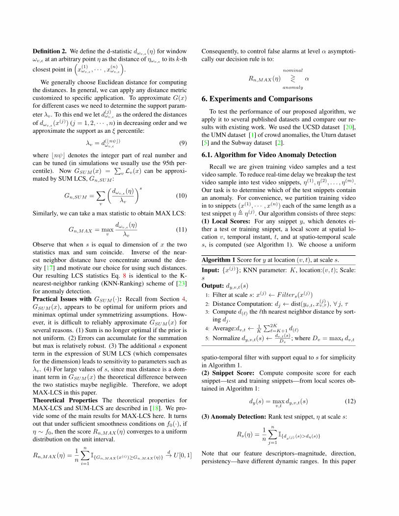
Recall we are given training video samples and a testvideo sample. To reduce real-time delay we breakup the testvideo sample into test video snippets, η(1), η(2), . . . , η(m).Our task is to determine which of the test snippets containan anomaly. For convenience, we partition training videoin to snippets (x(1), · · · , x(n)) each of the same length as atest snippet η , η(j). Our algorithm consists of three steps:(1) Local Scores: For any snippet y, which denotes ei-ther a test or training snippet, a local score at spatial lo-cation v, temporal instant, t, and at spatio-temporal scales, is computed (see Algorithm 1). We choose a uniform

Algorithm 1 Score for y at location (v, t), at scale s.

Input: x(j); KNN parameter: K, location:(v, t); Scale:sOutput: dy,v,t(s)

1: Filter at scale s: x(j) ← Filters(x(j))

2: Distance Computation: dj ← dist(yv,t, x(j)v,τ ), ∀ j, τ

3: Compute d(ℓ) the ℓth nearest neighbor distance by sort-ing dj .

4: Average:dv,t ← 1K

∑2Kℓ=K+1 d(ℓ)

5: Normalize dy,v,t(s)← dv,t(s)Dv

; where Dv = maxt dv,t

spatio-temporal filter with support equal to s for simplicityin Algorithm 1.(2) Snippet Score: Compute composite score for eachsnippet—test and training snippets—from local scores ob-tained in Algorithm 1:

dy(s) = maxv,t

dy,v,t(s) (12)

(3) Anomaly Detection: Rank test snippet, η at scale s:

Rs(η) =1

n

n∑j=1

Idx(j) (s)>dη(s)

Note that our feature descriptors–magnitude, direction,persistency—have different dynamic ranges. In this paper

we ranked separately with respect to the different descrip-tors. Anomalies are declared if the score at scale s, Rs(η),for any descriptor falls below the desired false alarm thresh-old, α. If an anomaly for a snippet is declared, the anomalyis localized by identifying the spatio-temporal locations,v, t in the snippet that achieve the maximum in Eq. 12.Tuning Parameters: Our algorithm requires only two pa-rameters, namely, K for KNN distance computation andscale s. It turns out that our results are generally robustto a wide range of K and is not an issue. In all our simu-lations we choose K to be about 50. Scale s can be dealtwith in two possible ways: (1) Compute ranks over differ-ent scales and declare anomaly if the rank at some scale fallsbelow the threshold. This procedure is conservative; Nev-ertheless, it controls false alarms at desired level asymp-totically. (2) Use context to determine sensible temporaland spatial scales. This idea has been used before by Conget. al. [8], who choose appropriate basis depending on thescenario. We choose small scales if small scale anomalies(abandoned or unusual objects) are important and chooselarger scales for spatial anomalies such as U-turns or globalchange in behavior.Computational Issues: KNN distance computation is ourmain bottleneck. It scales linearly with the number of 3Dbricks. To overcome this drawback recent approaches forcomputing approximate nearest neighbors based on localitysensitive hashing(LSH) [4] can be used. While we do notpresent results based on LSH here, in our preliminary ex-periments we have noticed that it can drastically reduce thecomputation time (scaling as fourth root of the number of3D bricks) with little loss in performance.

6.2. UCSD Ped1 dataset [20]

The UCSD Ped1 dataset contains 34 training clips ofnominal patterns and 36 testing clips of various abnormalevents, e.g. bicycles, skaters, carts, etc. Each clip has 200frames (20 seconds), with a 158 × 238 resolution. Thechallenge in this dataset is that the scenes are extremelycrowded. To apply our algorithm, first we calculated op-tical flow and aggregated optical flow into histogram andmagnitude features. We divided the videos into overlappingspatio-temporal blocks of 30pixels×20pixels×5frames (theblock size was chosen such that each block does not con-tain too many objects which may interfere with one another)and then we applied our algorithm on snippets consisting of5 frames. We also experimented with larger snippets andnoticed little performance degradation.

Some image results are shown in Figure 4. Our algo-rithm can detect different types of anomalies. In Figure 5,we compared ROC curves of our method with SRC pro-posed in [8] and MDT proposed in [15]. We also comparedour method with Social force and MPPCA, etc. It is easy tosee that our method outperforms all the other algorithms. In

50 100 150 200

20

40

60

80

100

120

140

(a)

50 100 150 200

20

40

60

80

100

120

140

(b)

50 100 150 200

20

40

60

80

100

120

140

(c)

50 100 150 200

20

40

60

80

100

120

140

(d)

Figure 4. Abnormal event detections for UCSD Ped1 datasets. Theobjects such as cars, bicycles, skaters are all well detected.

Table 1, some evaluation results are presented: the EqualError Rate (EER) (ours 16% < 19% [8]), and Area UnderCurve (AUC) (ours 92.7% > 86% [8]). From these com-parisons, we can conclude that our algorithm outperformsother state-of-the-art algorithms. One additional advantageof our algorithm is that while providing frame level results,we can also provide anomaly localization by back-tracingto the block with max statistics.

Method EER AUCMPPCA [15] 40% 59%SF [15] 31% 67.5%MDT [15] 25% 81.8%Sparse [8] 19% 86%Ours 16% 92.7%

Table 1. Quantitative comparison of our algorithm with [8] and[15]. EER is equal error rate and AUC is the area under ROC.

6.3. Subway dataset [2]

The subway dataset is obtained from Adam et al. [2]. Inour experiments, we used the “entrance gate” video whichis 1 hour 36 minutes long with 144249 frames. For ourexperiments, we applied a 96pixels ×96pixels ×50framesblock (2 seconds).

In Figure 6, a few detected abnormal frames are shownwith abnormal blocks marked red. In Figure 7 we comparethe frame level ROC curves with results in [8]. It is ob-vious that our algorithm outperforms SRC proposed in [8]significantly for the subway dataset.

0 0.2 0.4 0.6 0.8 10

0.1

0.2

0.3

0.4

0.5

0.6

0.7

0.8

0.9

1

False Positive

Tru

e P

ositi

ve

SparseMDTSocial ForceMPPCAOurs

Figure 5. The detection results of UCSD Ped1 dataset.

50 100 150 200 250 300 350 400 450 500

50

100

150

200

250

300

350

(a)

50 100 150 200 250 300 350 400 450 500

50

100

150

200

250

300

350

(b)

Figure 6. Abnormal event detections for Subway datasets.

0 0.2 0.4 0.6 0.8 10

0.2

0.4

0.6

0.8

1

False Positive

Tru

e P

ositi

ve

OursSparse

Figure 7. The detection results of Subway dataset.

6.4. UMN dataset [1]

The UMN dataset [1] consists of 3 different scenes ofcrowds of walking people who suddenly started running.Scene 1 contains 1450 frames, scene 2 contains 4415 framesand scene 3 contains 2145 frames all with a 320×240 reso-lution. We used a 80pixels×80pixels×45frames block andtrained our algorithm using first 600 frames of each sceneand use the others for testing.

In Figure 8, we demonstrate some detected abnor-mal frames using our proposed algorithm. Table 2 pro-vides quantitative comparisons to other state-of-the-art al-

50 100 150 200 250 300

50

100

150

200

(a)

50 100 150 200 250 300

50

100

150

200

(b)

50 100 150 200 250 300

50

100

150

200

(c)

Figure 8. Abnormal event detections for UMN datasets.

gorithms. Our proposed algorithm is comparable to [22]and [8], and outperforms [16]. Note that our method issimpler and requires little parameter tuning in comparisonto other methods. In Figure 9 we compare the ROC curveswith several other algorithms.

Method AUCChaotic Invariants [22] 99%Social Force [16] 96%Optical Flow [16] 84%Sparse [8] 97.5%Ours 98.5%

Table 2. Quantitative comparison of our algorithm with [8], [16]and [22]. AUC is the area under ROC.

0 0.1 0.2 0.3 0.40

0.2

0.4

0.6

0.8

1

False Positive

Tru

e P

ositi

ve

OursSparseSparse(Non−weight)

Figure 9. The detection results of UMN dataset.

6.5. Uturn dataset [5]

The Uturn dataset is made available to us by Benezethet al. [5]. It is a video of a junction with cars driving indifferent directions, trams passing by and pedestrians walk-ing about. The anomalous activities in this case are ille-gal U-turns and trams. The video contains 6057 frames. Ablock of 120pixels ×240pixels ×60 frames is adopted inour experiment. Anomalous frames are shown to illustratethe detected anomaly in Figure 10. The results are depictedin Figure 11. Also in the top panel of Fig. 11 illustrateshow direction histograms behave as a time series. The firstanomalous instance (marked as red in the truth) is the tram,where direction 1, 2, 7 and 8 has large intensity. The restof the anomalous instances are Uturns, where the features

corresponding to the U-turn is spread out in all of the first 5directions in the histogram. Both these types of anomaliesare distinct from normal activities.

50 100 150 200 250 300 350

50

100

150

200

(a)

50 100 150 200 250 300 350

50

100

150

200

(b)

50 100 150 200 250 300 350

50

100

150

200

(c)

50 100 150 200 250 300 350

50

100

150

200

(d)

Figure 10. Abnormal event detections for Uturn dataset. DepictsUturn and Tram anomalies on the same spatio-temporal block ondifferent frames.

Diretio

n H

isto

gra

ms

Uturn Histogram Illustration

1000 2000 3000 4000 5000 6000

1

2

3

4

5

6

7

8

Time

Tru

th

1000 2000 3000 4000 5000 6000

123

0 0.2 0.4 0.6 0.8 10

0.2

0.4

0.6

0.8

1

False Positive

Tru

e P

ositi

ve

ROC curve

Figure 11. The detection results of Uturn dataset.

References[1] Unusual crowd activity dataset. http://mha.cs.umn.

edu/Movies/Crowd-Activity-All.avi. 1, 5, 7[2] A. Adam, E. Rivlin, I. Shimshoni, and D. Reinitz. Ro-

bust real-time unusual event detection using multiple fixed-location monitors. PAMI, 30(3):555–560, 2008. 1, 2, 5, 6

[3] S. Ali and M. Shah. Floor fields for tracking in high densitycrowd scenes. ECCV, 2008. 1

[4] A. Andoni and P. Indyk. Near-optimal hashing algorithms forapproximate nearest neighbor in high dimensions. Commun.ACM, 51:117–122, January 2008. 6

[5] Y. Benezeth, P. Jodoin, V. Saligrama, and C. Rosenberger.Abnormal events detection based on spatio-temporal co-occurences. CVPR, 2009. 1, 2, 3, 5, 7

[6] B.Horn and B. Schunck. Determining optical flow. 17(1-3):185–203, 1981. 3

[7] O. Boiman and M. Irani. Detecting irregularities in imagesand in video. ICCV, 2005. 1, 2

[8] Y. Cong, J. Yuan, and J. Liu. Sparse reconstruction cost forabnormal event detection. CVPR, 2011. 1, 2, 6, 7

[9] W. Hu, X. Xiao, Z. Fu, D. Xie, T. Tan, and S. Maybank.A system for learning statistical motion patterns. PAMI,28(9):1450–1464, 2006. 1

[10] L. Itti and P. Baldi. A principled approach to detectingsurprising events in video. In in Proc. IEEE Conferenceon Computer Vision and Pattern Recognition (CVPR, pages631–637, 2005. 2

[11] F. Jiang, J. Yuan, S. Tsaftaris, and A. Katsaggelos. Anoma-lous video event detection using spatiotemporal context.Computer Vision and Image Understanding, 115(3):323–333, 2011. 1

[12] S. Kay. Fundamentals of Statistical Signal Processing: De-tection Theory. Prentice Hall, 1998. 4

[13] J. Kim and K. Grauman. Observe locally, infer globally: Aspace-time mrf for detecting abnormal activities with incre-mental updates. CVPR, 2009. 1, 2

[14] L. Kratz and K. Nishino. Anomaly detection inextremelycrowded scenes using spatio-temporal motion pattern mod-els. CVPR, 2009. 1, 2

[15] V. Mahadevan, W. Li, V. Bhalodia, and N. Vasconcelos.Anomaly detection in crowded scenes. CVPR, 2010. 1, 2,6

[16] R. Mehran, A. Oyama, and M. Shah. Abnormal crowd be-havior detection using social force model. CVPR, 2009. 1,7

[17] J. Qian and V. Saligrama. Graph construction for learning onunbalanced data. http://arxiv.org/abs/1112.2319, 2011. 5

[18] V. Saligrama and M. Zhao. Local anomaly detection. InAISTATS, 2012. 2, 5

[19] B. Scholkopf, J. Platt, J. Shawe-Taylor, A. Smola, andR. Williamson. Estimating the support of a high-dimensionaldistribution. Neural Computation, July 2001. 2

[20] UCSD. Anomaly detection dataset, 2010. http://www.svcl.ucsd.edu/projects/anomaly/dataset.htm. 5, 6

[21] X. Wang, X. Ma, and W. Grimson. Unsupervised activityperception in crowded and complicated scenes using hierar-chical bayesian models. PAMI, 31(3):539–555, 2009. 1

[22] S. Wu, B. Moore, and M. Shah. Chaotic invariants oflagrangian particle trajectories for anomaly detection incrowded scenes. CVPR, 2010. 7

[23] M. Zhao and V. Saligrama. Anomaly detection with scorefunctions based on nearest neighbor graphs. In NIPS, vol-ume 22, 2009. 2, 5