statistical evaluation methodology for surrogate endpoints
TRANSCRIPT

Statistical Evaluation Methodology for
Surrogate Endpoints in Clinical Studies
Wim Van der Elst

Acknowledgements
The research described in this thesis has received funding from the EuropeanUnion’s 7th Framework Programme for research, technological developmentand demonstration under the IDEAL Grant Agreement no 602552.
i

ii

List of publications
Materials covered in this dissertation:
Alonso, A. A., Van der Elst, W., Molenberghs, G., Burzykowski, T., &Buyse, M. (2016). An information-theoretic approach for the evaluation ofsurrogate endpoints based on causal inference. Biometrics, 72, 669–677.
Van der Elst, W., Molenberghs, G., & Alonso, A. A. (2016). Exploring therelationship between the causal-inference and meta-analytic paradigms forthe evaluation of surrogate endpoints. Statistics in Medicine, 35, 1281–1298.
Van der Elst, W., Hermans, L., Verbeke, G., Kenward, M. G., Nassiri, V., &Molenberghs, G. (2016). Unbalanced cluster sizes and rates of convergence inmixed-effects models for clustered data. Journal of Statistical Computationand Simulation, 86, 2123–2139.
Alonso, A. A., & Van der Elst, W. (2016). The history of surrogate endpointevaluation: single-trial methods. In A. A. Alonso et al. (Eds.), AppliedSurrogate Endpoint Evaluation Methods with SAS and R. New York: CRCpress.
Alonso, A. A., & Van der Elst, W. (2016). Multiple trial methods for twocontinuous outcomes. In A. A. Alonso et al. (Eds.), Applied SurrogateEndpoint Evaluation Methods with SAS and R. New York: CRC press.
Van der Elst, W., Alonso, A. A., & Molenberghs, G. (2016). The R pack-age Surrogate. In A. A. Alonso et al. (Eds.), Applied Surrogate EndpointEvaluation Methods with SAS and R. New York: CRC press.
iii

Alonso, A. A., Van der Elst, W., & Molenberghs, G. (2016). Validatingpredictors of therapeutic success: a causal inference approach. StatisticalModelling.
Alonso A. A., Van der Elst, W., Molenberghs, G., Burzykowski, T., & Buyse,M. (2015). On the relationship between the causal-inference and meta-analytic paradigms for the validation of surrogate endpoints. Biometrics,71, 15–24.
Alonso, A. A., & Van der Elst, W. (under revision). Evaluating multivariatepredictors of therapeutic success: A causal inference approach. StatisticalMethods in Medical Research.
Van der Elst, W., Molenberghs, G., Hilgers, R., Verbeke, G., & Heussen, N.(2017). Estimating the reliability of repeatedly measured endpoints basedon linear mixed-effects models. A tutorial. Pharmaceutical Statistics.
Alonso, A. A., Van der Elst, W., & Meyvisch, P. (2017). Assessing a sur-rogate predictive value: a causal inference approach. Statistics in Medicine.
Related publications:
Alonso, A. A., Van der Elst, W., & Meyvisch, P. (submitted). A maximum-entropy approach for the evaluation of surrogate endpoints based on causalinference. Journal of the American Statistical Association.
Van der Elst, W., & Molenberghs, G. (2016). Surrogate endpoints in rarediseases. In A. A. Alonso et al. (Eds.), Applied Surrogate Endpoint Evalu-ation Methods with SAS and R. New York: CRC press.
Alonso, A. A., Meyvish, P., & Van der Elst, W. (submitted). On the pos-sibility of finding a good surrogate. Biostatistics.
Van der Elst, W., Molenberghs, G., Vercruysse, S., & Alonso, A. A. (underrevision). On the use of surrogate endpoint validation methods in psychologyand the behavioural sciences. British Journal of Mathematical and StatisticalPsychology.
iv

Buyse, M., Molenberghs, G., Paoletti, X., Oba, K., Alonso, A., Van der Elst,W., & Burzykowski, T. (2015). Statistical evaluation of surrogate endpointswith examples from cancer clinical trials. Biometrical Journal, 58, 104–132.
Molenberghs, G., Alonso, A. A., Van der Elst, W., Burzykowski, T., &Buyse, M. (2015). Statistical evaluation of surrogate endpoints in clinicalstudies. In W. R. Young & D. Chen (Eds.), Clinical Trial Biostatistics andBiopharmaceutical Applications. New York: CRC press.
Alonso, A., and Van der Elst, W. (2016). Surrogate markers validation:The continuous-binary setting from a causal inference perspective. Technicalreport.
v

vi
Contents
1 General introduction 11.1 Surrogate endpoints . . . . . . . . . . . . . . . . . . . . . . . . 11.2 Earlier approaches to surrogate marker evaluation . . . . . . . 3
1.2.1 Prentice’s approach . . . . . . . . . . . . . . . . . . . . 31.2.2 The proportion of treatment effect explained . . . . . . 51.2.3 The relative effect and adjusted association . . . . . . . 71.2.4 The meta-analytic approach . . . . . . . . . . . . . . . . 9
1.3 Overview of the thesis . . . . . . . . . . . . . . . . . . . . . . . 12
2 Data sets and software tools 152.1 Data sets . . . . . . . . . . . . . . . . . . . . . . . . . . . . . . 15
2.1.1 Five clinical trials in schizophrenia . . . . . . . . . . . . 152.1.2 The opiate/heroin addiction trial . . . . . . . . . . . . 162.1.3 The age-related macular degeneration (ARMD) trial . . 172.1.4 The cardiac output experiment . . . . . . . . . . . . . . 17
2.2 Software tools . . . . . . . . . . . . . . . . . . . . . . . . . . . . 192.2.1 The R package Surrogate . . . . . . . . . . . . . . . . . 192.2.2 The R package EffectTreat . . . . . . . . . . . . . . . . 192.2.3 The R package CorrMixed . . . . . . . . . . . . . . . . . 20
I Issues in the evaluation of surrogate endpoints 21
3 Evaluating surrogacy in the normal-normal setting 233.1 Introduction . . . . . . . . . . . . . . . . . . . . . . . . . . . . . 23
vii

CONTENTS
3.2 Single-trial setting . . . . . . . . . . . . . . . . . . . . . . . . . 243.2.1 The causal inference approach . . . . . . . . . . . . . . 243.2.2 Average causal necessity and average causal sufficiency . 273.2.3 Individual causal effects versus expected causal effects . 293.2.4 Individual causal association: some identifiability issues 303.2.5 Individual causal association and adjusted association . 313.2.6 Plausibility of finding a good surrogate . . . . . . . . . . 35
3.3 Multiple-trial setting . . . . . . . . . . . . . . . . . . . . . . . . 373.3.1 Expected causal association . . . . . . . . . . . . . . . . 373.3.2 Individual causal association in a meta-analytic framework 383.3.3 Individual causal effects versus expected causal effects . 39
3.4 Case study: five clinical trials in schizophrenia . . . . . . . . . 443.4.1 The single-trial setting . . . . . . . . . . . . . . . . . . . 443.4.2 The multiple-trial setting . . . . . . . . . . . . . . . . . 583.4.3 Accounting for the sampling variability in the estimation
of ⇢S0T0 and ⇢S1T1 . . . . . . . . . . . . . . . . . . . . . 643.4.4 Conclusion . . . . . . . . . . . . . . . . . . . . . . . . . 64
3.5 Discussion . . . . . . . . . . . . . . . . . . . . . . . . . . . . . . 65
4 Evaluating surrogacy in the binary-binary setting 674.1 Introduction . . . . . . . . . . . . . . . . . . . . . . . . . . . . . 674.2 The causal inference framework . . . . . . . . . . . . . . . . . . 684.3 Individual causal association . . . . . . . . . . . . . . . . . . . 70
4.3.1 Information theory . . . . . . . . . . . . . . . . . . . . . 704.3.2 Definition of R2
H . . . . . . . . . . . . . . . . . . . . . . 714.3.3 Relationship between the individual causal association
and other metrics of surrogacy . . . . . . . . . . . . . . 724.3.4 Identifiability issues . . . . . . . . . . . . . . . . . . . . 74
4.4 The surrogate predictive function . . . . . . . . . . . . . . . . . 794.4.1 Definition . . . . . . . . . . . . . . . . . . . . . . . . . . 794.4.2 Relationship between the surrogate predictive function
and other metrics of surrogacy . . . . . . . . . . . . . . 814.4.3 Assessing the SPF . . . . . . . . . . . . . . . . . . . . . 81
4.5 Case study: a clinical trial in schizophrenia . . . . . . . . . . . 824.5.1 The BPRS as a surrogate for the PANSS . . . . . . . . 84
viii

CONTENTS
4.5.2 The BPRS as a surrogate for the CGI . . . . . . . . . . 934.6 Discussion . . . . . . . . . . . . . . . . . . . . . . . . . . . . . . 95
II Topics related to the evaluation of surrogates 99
5 Evaluating predictors of therapeutic success 1015.1 Introduction . . . . . . . . . . . . . . . . . . . . . . . . . . . . . 1015.2 A causal inference model . . . . . . . . . . . . . . . . . . . . . . 1025.3 Predictive causal association . . . . . . . . . . . . . . . . . . . . 1045.4 Predicting the individual causal treatment effect . . . . . . . . 1065.5 PCA: some indentifiability issues . . . . . . . . . . . . . . . . . 1075.6 Regression-based approach . . . . . . . . . . . . . . . . . . . . . 1085.7 Case Study: a clinical trial in opiate/heroin addiction . . . . . 110
5.7.1 Data description . . . . . . . . . . . . . . . . . . . . . . 1115.7.2 Regression approach . . . . . . . . . . . . . . . . . . . . 1125.7.3 Causal inference approach . . . . . . . . . . . . . . . . . 112
5.8 Discussion . . . . . . . . . . . . . . . . . . . . . . . . . . . . . . 117
6 Evaluating surrogacy in the meta-analytic framework: compu-tational issues 1216.1 Introduction . . . . . . . . . . . . . . . . . . . . . . . . . . . . . 1216.2 Linear mixed-effects models and convergence issues . . . . . . . 122
6.2.1 Earlier simulation studies . . . . . . . . . . . . . . . . . 1236.2.2 Potential relevance of balance in trial size . . . . . . . . 1236.2.3 Simulations . . . . . . . . . . . . . . . . . . . . . . . . . 124
6.3 Balanced cluster sizes and multiple imputation . . . . . . . . . 1296.3.1 Simulations . . . . . . . . . . . . . . . . . . . . . . . . . 129
6.4 Case studies . . . . . . . . . . . . . . . . . . . . . . . . . . . . . 1336.4.1 The ARMD trial . . . . . . . . . . . . . . . . . . . . . . 1386.4.2 Five clinical trials in schizophrenia . . . . . . . . . . . . 140
6.5 Discussion . . . . . . . . . . . . . . . . . . . . . . . . . . . . . . 141
7 Estimating reliability using mixed-effects models 1457.1 Conventional methods to estimate reliability . . . . . . . . . . . 1457.2 Relevance of reliability . . . . . . . . . . . . . . . . . . . . . . . 147
ix

CONTENTS
7.3 Estimating reliability using the linear mixed-effects model . . . 1487.3.1 The mean structure of the model . . . . . . . . . . . . . 1497.3.2 The covariance structure of the model . . . . . . . . . . 1507.3.3 Advantages of using linear mixed-effects models to estim-
ate reliability . . . . . . . . . . . . . . . . . . . . . . . . 1527.4 Case study: the cardiac output experiment . . . . . . . . . . . 152
7.4.1 Exploratory data analysis . . . . . . . . . . . . . . . . . 1527.4.2 The mean structure of the model . . . . . . . . . . . . . 1537.4.3 The covariance structure . . . . . . . . . . . . . . . . . . 157
7.5 Discussion . . . . . . . . . . . . . . . . . . . . . . . . . . . . . . 162
Appendices 167
x

List of Tables
3.1 Simulation results, single-trial scenario . . . . . . . . . . . . . . 353.2 Simulation results, multiple-trial setting scenario (i) . . . . . . 453.3 Simulation results, multiple-trial setting scenario (ii) . . . . . . 463.4 Simulation results, multiple-trial setting scenario (iii) . . . . . . 473.5 Simulation results, multiple-trial setting scenario (iv) . . . . . . 483.6 Simulation results, multiple-trial setting scenario (v) . . . . . . 493.7 Schizophrenia study. Summary statistics for ⇢� and ⇢M ac-
counting for sampling variability . . . . . . . . . . . . . . . . . 64
4.1 Distribution of � = (�T,�S)0. . . . . . . . . . . . . . . . . . . 69
4.2 R2H versus other metrics of surrogacy . . . . . . . . . . . . . . . 73
4.3 Distribution of Y . . . . . . . . . . . . . . . . . . . . . . . . . . 774.4 Schizophrenia study, binary-binary setting. Cross-tabulation of
the BPRS (S) versus PANSS (T ) outcomes . . . . . . . . . . . 834.5 Schizophrenia study, binary-binary setting. Cross-tabulation of
the BPRS (S) versus CGI (T ) outcomes . . . . . . . . . . . . . 834.6 Schizophrenia study, binary-binary setting, S = BPRS and T
= PANSS. SPF summary statistics when the sampling variab-ility in the marginal probabilities is not accounted for and isaccounted for . . . . . . . . . . . . . . . . . . . . . . . . . . . . 89
4.7 Schizophrenia study, binary-binary setting, S = BPRS and T =PANSS. R2
H results under different monotonicity scenarios . . . 90
5.1 Opiate/heroin study. Correlations between the pretreatmentpredictors and the true endpoints . . . . . . . . . . . . . . . . . 111
xi

LIST OF TABLES
5.2 Opiate/heroin study. Results of regression analysis . . . . . . . 1135.3 Opiate/heroin study. Summary statistics for R2
using differentcombinations of pretreatment predictors . . . . . . . . . . . . . 117
6.1 Convergence rates for the random-intercept models, reduced sur-rogate models, and surrogate models . . . . . . . . . . . . . . . 130
6.2 Mean (SD) number of iterations per convergence category forthe random-intercept models, the reduced surrogate models, andthe surrogate models . . . . . . . . . . . . . . . . . . . . . . . . 131
6.3 Hypothetical dataset. Number of observations per trial beforeand after imputation . . . . . . . . . . . . . . . . . . . . . . . . 132
6.4 Convergence rates for the surrogate evaluation models . . . . . 1346.5 Mean (SD) number of iterations per convergence category for
the surrogate models . . . . . . . . . . . . . . . . . . . . . . . . 1356.6 Bias, efficiency and MSE of the estimates of individual-level sur-
rogacy . . . . . . . . . . . . . . . . . . . . . . . . . . . . . . . . 1366.7 Bias, efficiency and MSE of the estimates of trial-level surrogacy 1376.8 ARDM study. Mixed-effects model convergence rates using the
unstructured factor analytic modeling strategies. . . . . . . . . 139
7.1 Summary of the covariance structures used in Models 1–3, andthe impact on the estimated reliabilities. . . . . . . . . . . . . . 151
7.2 The cardiac output experiment. Fractional polynomial results. 1547.3 The cardiac output experiment. Fit indices of the different mod-
els for the ZSV outcome. . . . . . . . . . . . . . . . . . . . . . . 161
xii

List of Figures
2.1 ARMD trial. Visual chart . . . . . . . . . . . . . . . . . . . . . 18
3.1 Simulation results in the single-trial setting . . . . . . . . . . . 363.2 Simulation results in the multiple-trial setting . . . . . . . . . . 503.3 Schizophrenia study, single-trial setting. Adjusted associations 513.4 Schizophrenia study, single-trial causal inference framework.
Histograms of ⇢� . . . . . . . . . . . . . . . . . . . . . . . . . . 523.5 Schizophrenia study, single-trial causal inference framework.
Causal diagrams . . . . . . . . . . . . . . . . . . . . . . . . . . 533.6 Schizophrenia study, single-trial causal inference framework.
Histograms of � . . . . . . . . . . . . . . . . . . . . . . . . . . . 543.7 Schizophrenia study, single-trial causal inference framework.
Histograms of ⇢2min . . . . . . . . . . . . . . . . . . . . . . . . . 563.8 Schizophrenia study, single-trial causal inference framework.
Causal diagrams for S = BPRS and T = CGI . . . . . . . . . 573.9 Schizophrenia study, meta-analytic framework. Plots of
individual- and trial-level surrogacy for S = BPRS and T =
PANSS . . . . . . . . . . . . . . . . . . . . . . . . . . . . . . . 593.10 Schizophrenia study, single-trial causal inference framework.
Histograms of ⇢M . . . . . . . . . . . . . . . . . . . . . . . . . . 603.11 Schizophrenia study, single-trial causal inference framework,
S = BPRS and T = CGI. Histograms of � and ⇢2min . . . . . . 613.12 Schizophrenia study, meta-analytic framework. Plots of
individual- and trial-level surrogacy for S = BPRS and T = CGI 62
xiii

LIST OF FIGURES
3.13 Schizophrenia study, multiple-trial causal inference framework.Causal diagrams for S = BPRS and T = CGI . . . . . . . . . . 62
3.14 Schizophrenia study, single-trial causal inference framework.Causal diagrams for S = BPRS and T = CGI . . . . . . . . . . 63
4.1 Schizophrenia study, binary-binary setting. Density of R2H for S
= BPRS and T = PANSS . . . . . . . . . . . . . . . . . . . . . 844.2 Schizophrenia study, binary-binary setting. Causal diagrams for
S = BPRS and T = PANSS . . . . . . . . . . . . . . . . . . . . 854.3 Schizophrenia study, binary-binary setting. SPF results for S =
BPRS and T = PANSS . . . . . . . . . . . . . . . . . . . . . . 884.4 Schizophrenia study, binary-binary setting. Densities of R2
H forS = BPRS and T = PANNS in the different montonicity scenarios 91
4.5 Schizophrenia study, binary-binary setting, S = BPRS and T =PANSS. SPF assuming monotonicity for S . . . . . . . . . . . . 92
4.6 Schizophrenia study, binary-binary setting. Density of R2H for S
= BPRS and T = CGI . . . . . . . . . . . . . . . . . . . . . . . 944.7 Schizophrenia study, binary-binary setting. SPF results for S =
BPRS and T = CGI . . . . . . . . . . . . . . . . . . . . . . . . 96
5.1 Opiate/heroin study. Histogram of R2 . . . . . . . . . . . . . . 115
5.2 Opiate/heroin study. Expected �T |S and their 95% supportintervals . . . . . . . . . . . . . . . . . . . . . . . . . . . . . . . 116
5.3 Distributions of R2 using different combinations of pretreatment
predictors . . . . . . . . . . . . . . . . . . . . . . . . . . . . . . 1185.4 Excel sheet for user-friendly prediction of �Tj | S and its 95%
support interval. . . . . . . . . . . . . . . . . . . . . . . . . . . 119
7.1 The cardiac output experiment. Individual profiles and meanvalues of the ZSV outcome as a function of time . . . . . . . . 154
7.2 The cardiac output experiment. Number of observations for theZSV outcome as a function of time of measurement. . . . . . . 155
7.3 The cardiac output experiment. Observed means as a function oftime of measurement and fitted fractional polynomial of degreeM = 3 . . . . . . . . . . . . . . . . . . . . . . . . . . . . . . . . 156
xiv

LIST OF FIGURES
7.4 The cardiac output experiment. Estimated reliabilities for ZSVbased on the different models . . . . . . . . . . . . . . . . . . . 159
7.5 The cardiac output experiment. Estimated reliabilities for ZSVat different time points and their 95% Confidence Intervals . . 160
7.6 Estimated reliabilities and 95% bootstrap-based Confidence In-tervals for ZSV based on the ‘full’ and the ‘reduced’ mixed-effectsmodels . . . . . . . . . . . . . . . . . . . . . . . . . . . . . . . . 165
xv

LIST OF FIGURES
xvi

List of Abbreviations
BPRS Brief psychiatric rating scaleCGI Clinical global impression
COWS Clinical opiate withdrawal scale
ECA Expected causal associationECE Expected causal effects
ECT Entropy concentration theoremICA Individual causal association
MI Multiple imputationMICA Meta-analytic individual causal association
MTS Multiple-trial setting
PANSS Positive and negative syndrome scalePCA Predictive causal association
PMSE Prediction mean squared error
RE Relative effect
S Surrogate endpointSPF Surrogate predictive functionSTS Single-trial setting
SUTVA Stable unit treatment value assumptionT True endpoint
Z Treatment indicatorZSV Electrical impedance tomography
xvii


Chapter 1
General introduction
The main focus of this thesis is on surrogate marker evaluation methods. Aswill be detailed in Section 1.1, a surrogate marker is essentially an endpointthat allows for predicting the effect of a treatment on the true endpoint (i.e.,the clinically most relevant endpoint). An overview and critical appraisal of themain surrogate evaluation paradigms that were developed earlier is providedin Section 1.2. In Section 1.3, an overview of the topics that are discussed inthe present thesis is provided.
1.1 Surrogate endpoints
An important factor that affects the duration, complexity, and cost of a clinicaltrial is the endpoint that is used to study the treatment’s efficacy (Burzykowski,Molenberghs and Buyse, 2005). In some situations, it is infeasible to use thetrue endpoint (i.e., the most credible indicator of the therapeutic response;Alonso et al., 2016). For example:
• the true endpoint may require a long follow-up time (e.g., survival time inoncology), such that the evaluation of the new therapy using this endpointwould be delayed and potentially confounded by other therapies,
• the true endpoint may have a low incidence (e.g., pregnancy in severeluteinizing hormone deficiency), such that the evaluation of the new ther-apy using this endpoint would result in a very large sample size,
1

CHAPTER 1. GENERAL INTRODUCTION
• the true endpoint may be costly to measure (e.g., magnetic resonanceimaging brain scans in mild cognitive impairment), such that the evalu-ation of the new therapy using this endpoint would be expensive.
In such situations, it can be an attractive strategy to substitute the true end-point by another endpoint that can be measured earlier (e.g., change in tumourvolume in oncology), that has a higher prevalence (e.g., follicular developmentin severe luteinizing hormone deficiency), or that can be measured more cheaply(e.g., cognitive change in mild cognitive impairment). Such a replacement out-come for the true endpoint is termed a ‘surrogate endpoint’.
Before a surrogate endpoint can replace the true endpoint in a clinical trial,it’s appropriateness has to be evaluated. It is a common misconception thatsurrogacy ‘automatically’ follows from the association between a candidate sur-rogate and the true endpoint. In the past, this misconception has had somesevere consequences. For example, the Food and Drug Administration (FDA)approved three drugs (i.e., encainide, flecainide, and moricizine) because oftheir capacity to suppress arrhythmias. As arrhythmia is known to be asso-ciated with a significant increase in death rates due to cardiac complications,it was assumed that these drugs would also reduce death rate. However, apost-marketing trial showed that the active-treatment death rate was actuallyhigher than the placebo death rate (CAST, 1989).
The mere correlation between two endpoints is thus not sufficient to evaluatethe appropriateness of a candidate surrogate (Fleming and DeMets, 1996).What is truly needed to replace the true endpoint by a surrogate endpoint ina clinical trial is that the treatment effect on the surrogate endpoint providesa good indication of the treatment effect on the true endpoint.
The formal evaluation of the appropriateness of a candidate surrogate en-dpoint is not a trivial task. Over the last few decades, various statisticalprocedures to achieve this aim have been proposed. In the next section, thesemethods are briefly reviewed.
2

CHAPTER 1. GENERAL INTRODUCTION
1.2 Earlier approaches to surrogate marker eval-
uation
1.2.1 Prentice’s approach
Prentice (1989) defined a surrogate endpoint as ‘a response variable for whicha test of the null hypothesis of no relationship to the treatment groups undercomparison is also a valid test of the corresponding null hypothesis based on thetrue endpoint’ (Prentice, 1989; pp. 432). This definition essentially requiresthat the surrogate endpoint S should capture any relationship between thetreatment Z and the true endpoint T (Lin, Fleming and De Gruttola, 1997).Symbolically, Prentice’s definition can be written as
f(S | Z) = f(S) , f(T | Z) = f(T ),
where f(S) and f(T ) denote the probability distributions of the random vari-ables S and T , and f(S | Z) and f(T | Z) denote the probability distributionsof S and T conditional on the value of Z, respectively. Notice that this defini-tion involves the triplet (T, S, Z), i.e., S is a surrogate for T only with respectto the effect of some specific treatment Z and not (necessarily) for a differenttreatment (except when S is a perfect surrogate for T , i.e., except when S andT are deterministically related).
Based on his definition of a surrogate endpoint, Prentice formulated fouroperational criteria that should be fulfilled for a good surrogate
f(S | Z) 6= f(S), (1.1)
f(T | Z) 6= f(T ), (1.2)
f(T | S) 6= f(T ), (1.3)
f(T | S, Z) = f(T | S). (1.4)
Thus, the treatment Z should have a significant effect on S (see (1.1)), thetreatment Z should have a significant effect on T (see (1.2)), S should have asignificant effect on T (see (1.3)), and the effect of the treatment Z on T shouldbe fully captured by S (see (1.4)).
For example, in the setting where both the surrogate and the true endpointsof a patient j (i.e., Sj and Tj) are normally distributed and Zj is a binary
3

CHAPTER 1. GENERAL INTRODUCTION
indicator for the treatment, the first two Prentice criteria (see (1.1)-(1.2)) canbe examined by fitting the following bivariate linear regression model
Sj = µS + ↵Zj + "Sj , (1.5)
Tj = µT + �Zj + "Tj , (1.6)
where the error terms "Sj and "Tj have a joint zero-mean normal distributionwith variance-covariance matrix
⌃ =
�SS �ST
�ST �TT
!. (1.7)
Further, the third and fourth Prentice criteria (see (1.3)-(1.4)) can be examinedby fitting the following univariate linear regression models
Tj = µ+ �Sj + "j , (1.8)
Tj = eµT + �SZj + �ZSj + e"Tj , (1.9)
where�S = � � �ST�
�1SS↵,
�Z = �ST��1SS ,
and the variance of e"T equals
�TT � �2ST�
�1SS .
To be in line with Prentice’s criteria, the hypotheses H0 : ↵ = 0, H0 : � = 0,and H0 : � = 0 in models (1.5)-(1.6) and (1.8) should be rejected, whereas thehypothesis H0 : �S = 0 in model (1.9) should not be rejected.
An appraisal of Prentice’s approach The Prentice criteria are intuitivelyappealing and straightforward to test, but there are some fundamental prob-lems that surround this approach.
First, the fourth Prentice criterion requires that the statistical test for the�S parameter is non-significant (see (1.9)). This criterion is useful to reject apoor surrogate endpoint (i.e., a surrogate for which �S 6= 0), but it is not suit-able to conclude that the candidate surrogate is appropriate (i.e., a surrogatefor which �S = 0). Indeed, in the Prentice framework one would have to accept
4

CHAPTER 1. GENERAL INTRODUCTION
the null hypothesis H0 : �S = 0 to conclude that the surrogate is appropriate,which is obviously not possible (Freedman, Graubard and Schatzkin, 1992).For example, the non-significant hypothesis test may always be the result of alack of statistical power due to an insufficient number of patients in the trial.
Second, even when lack of statistical power would not be an issue, the resultof the statistical test to evaluate the fourth Prentice criterion (i.e., H0 : �S = 0)cannot prove that the effect of the treatment Z on T is fully captured byS (Burzykowski, Molenberghs and Buyse, 2005; Frangakis and Rubin, 2002).Moreover, in any practical setting it would be more realistic to expect thata surrogate explains a part of the treatment effect on the true endpoint –rather than the full effect. This consideration led Freedman, Graubard andSchatzkin (1992) to the proposal that attention should be shifted away from thehypothesis-testing framework of Prentice (1989) (i.e., a yes/no all-or-nothingqualitative judgement of the appropriateness of a candidate S) to an estimationframework (i.e., a quantitative rating of the appropriateness of a candidateS). The proposal of Freedman, Graubard and Schatzkin (1992) is detailed inSection 1.2.2.
Third, it can be shown that Prentice’s operational criteria to evaluate acandidate S are only equivalent to his definition of a surrogate when both S
and T are binary variables. This implies that verifying the operational criteriadoes not guarantee that the surrogate truly fulfills the definition – except whenall members of the triplet (Z, T, S) are binary. For details, the reader is referredto Buyse and Molenberghs (1998).
Fourth, the Prentice criteria require that the treatment Z significantly af-fects both S and T (see (1.1)-(1.2)). Thus, the data of a clinical trial in whichthe treatment has no significant effect on both S and T cannot be used toevaluate a surrogate endpoint in Prentice’s approach.
1.2.2 The proportion of treatment effect explained
In view of the problems with the Prentice criteria, Freedman, Graubard andSchatzkin (1992) proposed to quantify surrogacy as the proportion of the effectof the treatment on T that is explained by S (the proportion explained, PE )
PE(T, S, Z) =
� � �S�
= 1�
�S�
, (1.10)
5

CHAPTER 1. GENERAL INTRODUCTION
where � is the estimate of the effect of the treatment on T without correctionfor S and �S is the estimate of the effect of the treatment on T with correctionfor S. The intuition behind the PE is that, if all treatment effect is mediatedby S (i.e., if �S = 0), then PE = 1. On the other hand, if there is no mediationat all (i.e., if � = �S), then PE = 0. Note that the fourth Prentice criterion isequivalent to the requirement that PE = 1.
An appraisal of the proportion explained As was also the case with thePrentice criteria, there are some fundamental issues with the PE.
First, the intuition behind the PE (i.e., that PE = 1 when all treatmenteffect is mediated by S and PE = 0 when there is no mediation) is flawedbecause �S is not necessarily zero when there is full mediation, and �, �Sare not necessarily equal when there is no mediation. As a result, the PE isnot confined to the unit interval and it is thus not truly a proportion in themathematical sense (i.e., it does not always holds that 0 PE 1).
Second, to be useful in practice a surrogate endpoint should allow for theprediction of the effect of Z on T based on the effect of Z on S (in a futureclinical trial). It is not clear how such a prediction can be made within the PEframework.
Third, the confidence interval of the PE tends to be wide. In fact, Freedman(2001) found that the ratio b�/s.e.(b�) should be � 5 (indicative of a very strongtreatment effect on T ) to achieve 80% power for a test of the hypothesis thatS explains more than 50% of the effect of Z on T . Arguably, such a strongrequirement makes the use of the PE infeasible in practice.
Fourth, the PE approach assumes that model (1.9) is the correct model(when S and T are continuous normally distributed endpoints). If this as-sumption is not correct (e.g., if the association between S and T depends onZ), the PE ceases to have a single interpretation and the surrogate evaluationprocess cannot be continued (Freedman, Graubard and Schatzkin, 1992).
Finally, the conceptual foundation of the PE (and the related fourth Pren-tice criterion) is problematic, because the treatment effect on T is obtainedafter conditioning on the post-randomisation S. Consequently, it cannot beconsidered to be a causal effect (Frangakis and Rubin, 2002).
6

CHAPTER 1. GENERAL INTRODUCTION
1.2.3 The relative effect and adjusted association
In view of the fundamental problems with the PE, Buyse and Molenberghs(1998) proposed two new quantities to assess surrogacy, i.e., the relative effect(RE ) and the adjusted association (�). In the setting where both S and T arecontinuous normally distributed endpoints, these metrics are computed as
RE(T, S, Z) =
�
↵, (1.11)
� = corr(S, T | Z) =
�STp
�SS�TT. (1.12)
The RE is the ratio of the effect of Z on T and the effect of Z on S. IfRE = 1, then the magnitude of the treatment effect on T is identical to themagnitude of the treatment effect on S. Notice that, in contrast to what wasthe case with the PE, the treatment effects involved in RE are not adjustedfor post-randomisation variables and thus these measures have a direct causalinterpretation. Indeed, ↵ and � are simply the average individual causal effectsof the treatment on S and T , respectively (see also Chapter 3). The adjustedassociation � quantifies how strongly S and T are associated at the level ofthe individual patients (after accounting for the treatment effect). If � = 1,then there exists a deterministic relationship between S and T – and thus thetrue endpoint for an individual patient can be perfectly predicted based onhis or her surrogate endpoint and the administered treatment. If � = 0, thenknowledge of S does not improve the prediction of T in an individual patient.
An appraisal of the adjusted association When both S and T are con-tinuous normally distributed endpoints, there are no issues with the adjustedassociation (�). Indeed, � is simply the correlation between S and T adjus-ted for Z. This metric has desirable properties, i.e., it always remains withinthe unit interval, it generally has a small confidence interval (because there issufficient individual-level replication in most clinical trials), and it is straight-forward to compute and interpret.
However, when we move away from the situation were both S and T arecontinuous normally distributed endpoints, it is no longer clear how � shouldbe quantified. For example, in the mixed continuous-binary setting (i.e., S iscontinuous and T is binary), a bivariate probit model can be used in which � is
7

CHAPTER 1. GENERAL INTRODUCTION
defined as the correlation between a latent continuous variable that is assumedto underlie the observed discretized endpoint T and the continuous endpointS. Or alternatively, a bivariate Plackett-Dale model can be used in which � isdefined as the global odds ratio between S and T (Geys, 2005). A variety ofother metrics have been proposed to quantify � in other settings (for details,see Burzykowski, Molenberghs and Buyse, 2005), but it would be desirable tohave a single unifying framework available that allows for the quantificationof � in a wide variety of settings. The more recently proposed information-theoretic surrogate evaluation approach provides such a framework (Alonsoand Molenberghs, 2007; see also Chapters 3 and 4).
An appraisal of the relative effect The main motivation to evaluate asurrogate endpoint is to be able to predict the unobserved effect of Z on T
in a future clinical trial i = 0 (i.e., b�0) based on the observed (estimated)effect of Z on S (i.e., b↵0). The RE allows for such a prediction (providedthat RE is sufficiently precisely estimated), but doing so requires a strong andunverifiable assumption. Often, it is assumed that the relationship between b�and b↵ is multiplicative (which comes down to a regression line through (0, 0)
and⇣b�, b↵
⌘). In other words, it is assumed that RE remains constant across
clinical trials. Of course, the validity of the constant RE assumption cannotbe verified in a setting where the data of only one clinical trial are available.
Second, in contrast to � (which has an interpretation in terms of the strengthof the treatment-corrected association between S and T ), the RE has no directinterpretation in terms of the strength of the association between � and ↵. Thisissue arises from the fact that a single clinical trial replicates patients – andthus a basis is provided for inference regarding patient-related characteristics– but not characteristics of the trial itself (i.e., ↵ and �). Thus, even whenthe unverifiable constant RE assumption would not be an issue, there still is aproblem (Molenberghs et al., 2013). To see this more clearly, expression (1.11)is rewritten as � = RE ⇤ ↵ and an intercept is included (to make it moregeneral), yielding � = µ + RE ⇤ ↵. The question now rises how accurate thislinear relationship is. To study this in proper statistical terms, a final rewriteis necessary by adding an error term " in the previous expression, yielding� = µ + RE ⇤ ↵ + " (where it is assumed that " ⇠ N
�0, �2
�). Obviously, �2
can only be estimated when there is appropriate replication of the pair (�, ↵).
8

CHAPTER 1. GENERAL INTRODUCTION
Put in another way: the data of multiple clinical trials are required to quantifythe accuracy by which � can be estimated.
1.2.4 The meta-analytic approach
The issues discussed in Section 1.2.3 led to the suggestion that there shouldbe adequate replication at the level of the clinical trial – in addition to thereplication at the level of the individual patients. Let us now assume thatthe data of i = 1, . . . , N trials are available, in the ith of which j = 1, . . . , ni
patients are enrolled. Denote by Tij and Sij the normally distributed trueand surrogate endpoints for patient j in trial i, respectively, and by Zij the(binary) indicator variable for the new treatment. In this setting, Buyse etal. (2000) proposed to evaluate surrogacy based on the following linear mixed-effects model
8<
:Sij = µS +mSi + (↵+ ai)Zij + "Sij ,
Tij = µT +mTi + (� + bi)Zij + "Tij ,(1.13)
where µS , µT are the fixed intercepts for S and T , mSi, mTi are the cor-responding random intercepts, ↵, � are the fixed treatment effects for S andT , and ai, bi are the corresponding random treatment effects. The vector ofthe random effects (mSi, mTi, ai, bi) is assumed to be mean-zero normallydistributed with variance-covariance matrix D
D =
0
BBBBB@
dSS dST dSa dSb
dTT dTa dTb
daa dab
dbb
1
CCCCCA. (1.14)
The error terms "Sij and "Tij in (1.13) are assumed to be mean-zero normallydistributed with variance-covariance matrix ⌃
⌃ =
�SS �ST
�TT
!. (1.15)
Metrics of surrogacy In the meta-analytic framework, surrogacy is quanti-fied based on two metrics, i.e., the trial- and individual-level coefficients of de-termination. The trial-level coefficient of determination quantifies the strength
9

CHAPTER 1. GENERAL INTRODUCTION
of the association between the treatment effects on T (i.e., �i = �+ bi) and thetreatment effects on S (i.e., ↵i = ↵+ ai) in the N different trials
R2trial = Rbi|mSi, ai
=
dSb
dab
!T dSS dSa
dSa daa
!�1 dSb
dab
!
dbb. (1.16)
All quantities in (1.16) are based on the D matrix (1.14). The R2trial value is
unitless and lies within the unit interval when the D matrix is positive definite.A 95% confidence interval around R2
trial can be computed as
R2trial ± 1.96
s4R2
trial
�1�R2
trial
�2
N � 3
, (1.17)
where the variance of R2trial is estimated using the Delta method and N refers
to the total number of clinical trials that were available in the analysis. Fora derivation of (1.17), the reader is referred to Cortiñas et al. (2008). AnR2
trial that is close to 1 indicates that there is a strong association between thetreatment effects on S and T in the N different trials. A surrogate is calledtrial-level valid when this is the case. The term ‘trial-level’ surrogacy refers tothe fact that the treatment effects on S and T (i.e.,
⇣b↵i, b�i
⌘) are observed at
the level of the clinical trial.The individual-level coefficient of determination quantifies the strength of
the association between S and T in the different patients (after adjustment forboth the trial- and treatment-effects)
R2indiv = R2
"Tij |"Sij=
�2ST
�SS�TT, (1.18)
where the quantities in (1.18) are based on the ⌃ matrix (1.15). A 95% con-fidence interval around R2
indiv can be obtained as
R2indiv ± 1.96
s4R2
indiv
�1�R2
indiv
�2
Ntotal � 3
,
where the variance of R2indiv is estimated using the Delta method and Ntotal
refers to the total number of patients in the study. An R2indiv close to 1 indicates
that there is a strong association between S and T at the level of the individualpatients (after adjusting for treatment- and trial-effects). A surrogate is calledindividual-level valid when this is the case. The term ‘individual-level’ refersto the fact that S and T are observed at the level of the individual patients.
10

CHAPTER 1. GENERAL INTRODUCTION
An appraisal of the meta-analytic approach The meta-analytic ap-proach provides an elegant and statistically-sound framework, but its practicaluse is hampered by the fact that data of multiple clinical trials are neededfor the analysis. Indeed, it is often not feasible to have a sufficient amount oftrial-level replication. To this end, several authors have proposed the use ofalternative clustering units (e.g., the hospitals in which patients are treated).The choice for a particular clustering unit may depend on several considera-tions, such as the information that is available in the dataset, experts’ opinionsregarding the most suitable clustering unit, and the number of patients per clus-tering unit (Burzykowski, Molenberghs and Buyse, 2005). Simulation studieshave shown that the impact of shifting between clustering units (e.g., usinghospital instead of trial) on the estimated R2
trial is small when the magnitudeof the variability in the treatment effects at the different levels (clinical trial,hospital) is roughly similar. However, when there are large differences in themagnitude of this variability, the impact of shifting between clustering units onthe estimated R2
trial can be substantial and thus caution is needed (for details,see Cortiñas et al., 2004).
A second issue with the meta-analytic approach is that fitting model (1.13)is computationally challenging – even if the data of a large number of trials isavailable (see also Chapter 6). To this end, several simplifying model-fittingapproaches were proposed. For example, Tibaldi et al. (2003) recommendedthe use of fixed-effect models instead of mixed-effects models, because bothapproaches yield comparable results whilst the fixed-effect models are substan-tially easier to fit and computationally less demanding. This recommendation ishowever based on the setting where there are no missing data, and the situationmay be different for incomplete data. Indeed, non-likelihood based models can-not handle incomplete data very well, so patients who have a missing value foreither S or T (or for Z, but this situation is less likely to occur) are discardedfrom the analyses. Such a complete case analysis is only unbiased when theresponses are Missing Completely At Random (MCAR, i.e., the probabilityof an observation being missing is independent of the observed and the unob-served responses) (Verbeke and Molenberghs, 2000; Molenberghs and Kenward,2007). MCAR is a strong assumption that is often not fulfilled in practice. Forexample, consider a typical surrogate marker evaluation setting in which T isdistant in time. A poor outcome on S may be associated with a higher prob-
11

CHAPTER 1. GENERAL INTRODUCTION
ability of drop-out (i.e., a missing T value) - and thus the MCAR assumptionmight be violated. In contrast to fixed-effect models, the use of mixed-effectsmodels has the advantage (1) that all available observations are used in theanalyses (provided that Z is not missing), and (2) that the missingness is ig-norable under MCAR and under Missing At Random missingness mechanisms(MAR, i.e., the probability of an observation being missing is independent ofthe unobserved outcomes conditional on the observed data; Molenberghs andKenward, 2007). The MAR assumption is more realistic than the MCAR as-sumption in most situations. For example, in the previous example where apoor outcome on S was associated with a higher probability of drop-out, theMCAR assumption is violated whilst the MAR assumption is not.
1.3 Overview of the thesis
In Chapter 2 of this thesis, a number of datasets and R software packagesare introduced. The datasets will be used to exemplify the methodology thatwas developed in the current thesis. This methodology was also implemen-ted in three R packages, i.e., the Surrogate, EffectTreat, and CorrMixed pack-ages (available for download at CRAN). A detailed account on how the resultsof the case study analyses that are described throughout this thesis can bereplicated using the R packages is available in an online Appendix. The on-line appendix can be downloaded at https://dl.dropboxusercontent.com/u/8416806/PhD_Appendix.pdf.
The main focus of Part I of this thesis is on new surrogate evaluationmethodology. The seminal work of Prentice (1989), Freedman, Graubard andSchatzkin (1992), Buyse and Molenberghs (1998), and Buyse et al. (2000) hasset the scene for a large research line into surrogate marker evaluation meth-ods. The different methods can be classified along two dimensions, taking intoaccount (i) whether they use information from a single clinical trial or frommultiple clinical trials, and (ii) whether they focus on individual or on expec-ted causal treatment effects (Joffe and Greene, 2009). When the focus is onindividual causal effects, it is assumed that each patient j has two potentialoutcomes for the true endpoint T and two potential outcomes for the surrog-ate endpoint S: an outcome T0j that would be observed under the controltreatment (Zj = 0) and an outcome T1j that would be observed under the ex-
12

CHAPTER 1. GENERAL INTRODUCTION
perimental treatment (Zj = 1) – and similarly for S. These are called ‘potentialoutcomes’, because they represent the outcomes that could have been observedif the patient had received the control treatment (then T0j and S0j are ob-served) or the experimental treatment (then T1j and S1j are observed). In thisframework, individual causal effects are typically defined as �Tj = T1j � T0j
and �Sj = S1j � S0j , and a ‘good’ surrogate endpoint should allow for anaccurate prediction of �Tj based on �Sj . On the other hand, expected causaltreatment effects refer to the averaged individual causal treatment effects, i.e.,� = E (Tj |Zj = 1)�E (Tj |Zj = 0) and similarly for ↵. In the latter framework,a ‘good’ surrogate is one where � can be accurately predicted based on ↵ (whichrequires trial-level replication unless one is willing to make strong assumptions,see Section 1.2.4). In Chapter 3 of this thesis, new metrics of surrogacy basedon individual causal effects in both the single- and multiple-trial settings areproposed in the scenario where both the surrogate and the true endpoints arenormally distributed variables. Further, the relationship between the metricsof surrogacy based on individual and expected causal effects will be exploredusing theoretical results and simulations. In Chapter 4, the causal inferenceframework will be used to establish metrics of surrogacy in the scenario whereboth endpoints are binary variables.
In Part II of this thesis, several topics that are related to surrogate endpointevaluation methods are considered. In particular, the focus of Chapter 5 is on‘personalized medicine’. The concept of personalized medicine refers to theidea that a medical treatment should be tailored to the individual patients’characteristics, as opposed to the practice where all patients with the samedisease receive the same treatment (i.e., the treatment that works best ‘onaverage’ in the population). For example, the FDA has recently approved anumber of cancer drugs for use in patients whose tumours have specific geneticcharacteristics but not for other patients who have a similar tumour with adifferent genetic fingerprint (FDA, 2013). The statistical challenges that areencountered in a surrogate evaluation setting and in a personalized medicinesetting are similar. As will be detailed in Chapter 5, The causal inference modelthat is used in a surrogate evaluation setting (see Chapters 3 and 4) can alsobe ‘translated’ into a personalized medicine context.
The meta-analytic surrogate evaluation approach (see Section 1.2.4)provides an elegant formalism in which two levels of surrogacy are distin-
13

CHAPTER 1. GENERAL INTRODUCTION
guished, i.e., trial-level surrogacy (which essentially quantifies the strengthof the association between the expected causal treatment effects on S andT ), and individual-level surrogacy (which essentially quantifies the treatment-and trial-corrected strength of association between S and T ). To estimateindividual- and trial-level metrics of surrogacy, a linear mixed-effects modelis fitted. Unfortunately, in real-life surrogate evaluation settings, convergenceproblems tend to be prevalent (see Section 1.2.4). In Chapter 6, simulationstudies are used to examine the factors that affect model convergence, anda multiple imputation-based approach to reduce model convergence issues isproposed.
Finally, in the meta-analytic surrogate evaluation approach, one of the mainmetrics of interest is the coefficient of individual-level surrogacy (see Section1.2.4). A psychometric concept that is related to individual-level surrogacyis reliability, which quantifies the reproducibility (or, predictability) of twoor more outcomes that are repeatedly measured within the same subject. InChapter 7, the focus will be on the use of linear mixed-effects model to estimatereliability in a flexible way.
14

Chapter 2
Data sets and software tools
2.1 Data sets
2.1.1 Five clinical trials in schizophrenia
This dataset combines the data that were collected in five double-blind ran-domized clinical trials. In these trials, the objective was to examine the efficacyof risperidone to treat schizophrenia. Schizophrenia is a mental disease that ishallmarked by hallucinations and delusions (American Psychiatric Association,2000).
In each trial, the Clinical Global Impression (CGI; Guy, 1976), Brief Psychi-atric Rating Scale (BPRS; Overall and Gorham, 1962), and Positive and Negat-ive Syndrome Scale (PANSS; Singh and Kay, 1975) were administered. Theseinstruments are clinical rating scales that are routinely used to assess symptomseverity in patients with schizophrenia (Mortimer, 2007). The patients in thedifferent trials were administered the experimental treatment risperidone or anactive control treatment (e.g., haloperidol, levomepromazine, or perphenazine)for four to eight weeks. The main endpoints of interest were the change in theCGI score (= CGI score at the end of the treatment - CGI score at the start ofthe treatment), the change in the PANSS score, and the change in the BPRSscore. A total of 2, 128 patients participated in the five trials, of whom 1, 591
patients received risperidone and 537 patients were given an active control.The patients were treated by a total of N = 198 psychiatrists. Each of the
15

CHAPTER 2. DATA SETS AND SOFTWARE TOOLS
psychiatrists treated between ni = 1 and 52 patients.In Chapter 3, it will be examined whether the change in the BPRS score is
a good surrogate for the change in the PANSS score, and whether the change inthe BPRS score is a good surrogate for the change in the CGI score. In clinicalpractice, the CGI, BPRS, and PANSS change scores are often dichotomizedto reflect the presence or absence of clinically relevant change in schizophrenicsymptomatology. To this end, clinically relevant change is typically defined asa reduction of 20% or more in the BPRS/PANSS scores (i.e, 20% reductionin posttreatment scores relative to baseline scores), or a change of more than3 points on the CGI scale (posttreatment scores compared to baseline; Kaneet al., 1988; Leucht et al., 2005). In Chapter 4, it will be examined whetherclinically relevant change on the BPRS score is a good surrogate for clinicallyrelevant change on the PANSS score.
2.1.2 The opiate/heroin addiction trial
The data come from a randomized clinical trial in which the clinical utilityof buprenorphine/naloxone (experimental treatment) was compared to clonid-ine (control treatment) for a short-term (13-day) opiate/heroin detoxificationtreatment.
A total of 335 patients took part in the study, of whom 106 patients re-ceived the active control and 229 patients received the experimental treatment.Study drop-out was substantial, i.e., only 104 patients completed the study. Inall patients, pretreatment opium craving, heroin use, and opiate withdrawalsymptoms were assessed. Opium craving was measured by means of a visualanalogue scale (score range [0; 100]). Heroin use in the 30-day interval priorto the start of the treatment was measured using a standardized question-naire. Opiate withdrawal symptoms were measured using the clinical opiatewithdrawal scale (COWS). The COWS is an 11-item interviewer-administeredquestionnaire that was designed to provide a description of the signs and symp-toms of opiate withdrawal like, e.g., sweating, runny nose, etc (score range[52; 200]). Treatment success was evaluated based on the number of days thata patient used heroin in a 30-day post-treatment interval in a personalizedmedicine setting.
In Chapter 5, the opiate/heroin addiction trial data will be used to examine
16

CHAPTER 2. DATA SETS AND SOFTWARE TOOLS
whether treatment success can be predicted based on the pretreatment variablesopium craving, heroin use, and opiate withdrawal symptoms.
2.1.3 The age-related macular degeneration (ARMD)
trial
The objective of this randomized clinical trial was to examine the efficacy ofinterferon-↵ to treat age-related macular degeneration (ARMD). ARMD is amedical condition in which patients progressively lose vision (PharmacologicalTherapy for Macular Degeneration Study Group, 1997). In the ARMD trial,visual acuity was examined using standardized vision charts that display lineswith five letters of decreasing sizes (see Figure 2.1). The patients had to readthese letters from top (largest letters) to bottom (smallest letters). Visualacuity was quantified as the total number of letters that were correctly read bya patient.
In Chapter 6, the ARMD dataset will be analysed. In particular, it will beexamined whether change in visual acuity 24 weeks after starting the treatmentis a good surrogate for the change in visual acuity 52 weeks after the start of thetreatment. A total of 240 patients participated in the ARMD trial, of whom190 patients had complete data (i.e., no missing values for visual acuity after 24or 52 weeks). The data of 9 patients were excluded from the analysis, becausethey were enrolled in a center (hospital) where all patients were assigned to thesame treatment arm. Thus, the data of a total of 181 patients from 36 centerswere used in the analyses. A total of 84 and 97 patients were enrolled in theplacebo and interferon-↵ treatment conditions, respectively.
2.1.4 The cardiac output experiment
Pikkemaat et al. (2014) performed an experiment where the cardiac output andstroke volume of 14 pigs was changed by increasing positive end-expiratorypressure (PEEP) levels (0, 5, 10, 15, 20, and 25 cm H2O). The number oftimes that a particular PEEP level was used varied from animal to animal.For each PEEP level, stroke volume was measured by electrical impedancetomography (ZSV). In each animal, four identical experiments were conducted(referred to as Cycles 1 to 4). The number of repeated ZSV measurementsacross PEEP levels and cycles in an animal ranged between 9 and 47. All the
17

CHAPTER 2. DATA SETS AND SOFTWARE TOOLS
V A L I DA T I O NO F S U RR O G A T
E M A R K
E R S I N
R A N D O
M I Z E D
E X P E R
I M E N T
Figure 2.1: Age-related macular degeneration (ARMD) trial. Visual chart.
18

CHAPTER 2. DATA SETS AND SOFTWARE TOOLS
measurements are approximately equally spaced. The data of 2 animals couldnot be evaluated due to technical reasons and the data of these animals werediscarded. In Chapter 7, the cardiac output experiment data will be used toestimate the reliability (i.e., temporal stability) of ZSV.
2.2 Software tools
2.2.1 The R package Surrogate
The surrogate evaluation methodology that is detailed in Part I of this thesis(Chapters 3 and 4) is implemented in the R package Surrogate (available fordownload at CRAN). The package also contains the data of the schizophreniaand ARMD case studies. A detailed account on how the results of the casestudy analyses that are described in Chapters 3 and 4 can be replicated usingthe package is available in an online Appendix that accompanies this thesis (seeChapters 1 and 2 of the online Appendix). The online appendix can be down-loaded at https://dl.dropboxusercontent.com/u/8416806/PhD_Appendix.pdf.
2.2.2 The R package EffectTreat
The methodology to evaluate putative predictors of treatment success (seeChapter 5 of this thesis) is implemented in the R package EffectTreat (avail-able for download at CRAN). A detailed account on how the results of theopiate/heroin addiction case study analysis described in Chapter 5 can be rep-licated using the package is available in the online Appendix that accompaniesthis thesis (see Chapter 3 of the online Appendix).
Note that opiate/heroin trial data are not included in the EffectTreatpackage because they are not in the public domain. After registration, thedata can be downloaded from the National Institute on Drug Abuse web-site (https://www.drugabuse.gov; studies NIDA-CTN-0001 and NIDA-CTN-0002).
19

CHAPTER 2. DATA SETS AND SOFTWARE TOOLS
2.2.3 The R package CorrMixed
The methodology to estimate reliability based on mixed-effects models (seeChapter 7 of this thesis) is implemented in the R package CorrMixed (availablefor download at CRAN). A detailed account on how the results of the cardiacoutput experiment described in Chapter 7 can be replicated using the packageis available in the online Appendix (see Chapter 4 of the online Appendix).
20

Part I
Issues in the evaluation of
surrogate endpoints
21


Chapter 3
Evaluating surrogacy in the
normal-normal setting based
on causal inference and meta-
analytic approaches
3.1 Introduction
As stated in Chapter 1, the use of a surrogate endpoint (S) can be an appealingstrategy to evaluate a new treatment (Z) when the true endpoint (T ) is difficultto assess. However, before a candidate S can replace T in a clinical study, itneeds to be statistically evaluated. The statistical evaluation of a candidate S
is not a trivial endeavour, and different strategies have been developed for thispurpose. Most of these methods can be classified along two dimensions, takinginto account (i) whether they use information from a single or from multipleclinical trials, and (ii) whether they focus on individual or on expected causaleffects (Alonso et al., 2016; Burzykowski, Molenberghs and Buyse, 2005; Bakerand Kramer, 2015; Conlon, Taylor and Elliott, 2014; Li et al., 2011).
In the present chapter, the conceptual frameworks that underlie the sur-rogate evaluation methodology based on individual and expected causal effectsin both the single- and the multiple-trial settings are detailed (Sections 3.2
23

CHAPTER 3. EVALUATING SURROGACY IN THE NORMAL-NORMALSETTING
and 3.3, respectively). Even though the causal inference paradigm is typicallyframed into the single-trial setting (STS), it is shown that this methodologycan also be embedded in the multiple-trial setting (MTS). Further, the rela-tionship between the causal inference and meta-analytic paradigms in the STSand MTS is studied using theoretical elements and simulations. The data of acase study are analysed in Section 3.4, and the some additional remarks andcritical comments are provided in Section 3.5.
3.2 Single-trial setting
3.2.1 The causal inference approach
We start by considering the STS, i.e., the setting where the inclusion andexclusion criteria of the clinical trial characterize a well-defined population inwhich the surrogate evaluation exercise is framed. Further, it will be assumedthat merely two treatments are under evaluation (Z = 0/1) in a parallel studydesign.
For the sake of simplicity, the focus will temporarily be restricted to T
alone. Following Rubin’s model for causal inference (Rubin, 1986), it will beassumed that each patient j has two potential outcomes for T : an outcomeT0j that would be observed under the control treatment condition (Zj = 0)and an outcome T1j that would be observed under the experimental treatmentcondition (Zj = 1). T0j and T1j are potential outcomes in the sense thatthey represent the outcomes of the patient had he or she received the control(Zj = 0) or the experimental treatment (Zj = 1), respectively. The so-calledfundamental problem of causal inference is that typically only one of T0j andT1j is observed in practice (Holland, 1986).
If we denote by Tj the observed outcome T for patient j then, under thestable unit treatment value assumption (SUTVA), Tj = ZjT1j + (1 � Zj)T0j .The SUTVA assumption underlays most work in the causal inference frame-work. In line with Rubin (1986), SUTVA can be defined in the following way:(i) the value of T for a patient j when exposed to treatment Z will be thesame no matter what mechanism is used to assign the treatment to patient j,and (ii) the value of T for patient j when exposed to treatment Z will be thesame no matter what treatments the other patients receive. Depending on the
24

CHAPTER 3. EVALUATING SURROGACY IN THE NORMAL-NORMALSETTING
setting at hand, SUTVA may or may not be a valid assumption. For example,condition (ii) could be violated in a flu vaccine study where the experimentaltreatment is the flu vaccine, the control treatment is placebo, and the potentialoutcomes are hospitalization status under the different treatment conditions.
Based on the vector of potential outcomes (T0j , T1j), the individual causaleffect of the treatment on a patient can be defined as �Tj = T1j � T0j andthe expected causal effect in the population under study as � = E (T1j � T0j).Unlike the individual causal effects, the expected causal effect is identifiablefrom the data under fairly general conditions. Indeed, � = E (Tj |Zj = 1) �
E (Tj |Zj = 0) when SUTVA holds and when it can be assumed that Zj ?
(T0j , T1j). The E (Tj |Zj = 0) and E (Tj |Zj = 1) quantities can be estimatedusing the observed means of Tj in the control and experimental treatmentgroups, respectively. Due to the random treatment allocation, the latter as-sumption of independence can often be guaranteed in clinical trials.
The distribution of the vector of potential outcomes is less relevant forthe estimation of expected causal effects, but it plays an important role whenindividual causal effects are considered. To that end, let us now consider thefull vector of potential outcomes Y j = (T0j , T1j , S0j , S1j)
0. It will be assumedthat Y j ⇠ N (µ,⌃), where µ = (µT0 , µT1 , µS0 , µS1)
0 and
⌃ =
0
BBBBB@
�T0T0 �T0T1 �T0S0 �T0S1
�T0T1 �T1T1 �T1S0 �T1S1
�T0S0 �T1S0 �S0S0 �S0S1
�T0S1 �T1S1 �S0S1 �S1S1
1
CCCCCA.
Let us now consider the vector of individual causal effects �j = (�Tj ,�Sj)0.
Given the aforementioned distributional assumptions, one has
�j = AY j =
T1j � T0j
S1j � S0j
!⇠ N (µ�,⌃�) , (3.1)
where ⌃� = A⌃A0, µ� = (�,↵)0 with � = E(�Tj) = µT1 � µT0 , ↵ =
E(�Sj) = µS1 � µS0 and
A =
�1 1 0 0
0 0 �1 1
!.
25

CHAPTER 3. EVALUATING SURROGACY IN THE NORMAL-NORMALSETTING
Intuitively, if S is a good surrogate for T , then �Sj should convey a substantialamount of information about �Tj . The amount of uncertainty in �Tj that isexpected to become removed when the value of �Sj becomes known is referredto as the mutual information. In the normal setting the concepts of mutualinformation and correlation are equivalent, and, therefore, it can be arguedthat the assessment of surrogacy can be based on the correlation between theindividual causal effects �Tj and �Sj . Along these lines, the individual causalassociation (ICA) is defined as ⇢� = corr (�Tj ,�Sj). It can easily be shownthat
⇢� =
p
�T0T0�S0S0⇢T0S0 +p
�T1T1�S1S1⇢T1S1 �p
�T1T1�S0S0⇢T1S0 �p
�T0T0�S1S1⇢T0S1q��T0T0 + �T1T1 � 2
p
�T0T0�T1T1⇢T0T1
� ��S0S0 + �S1S1 � 2
p
�S0S0�S1S1⇢S0S1
� ,
(3.2)
where ⇢XY denotes the correlation between the potential outcomes X and Y .ICA is also a measure of prediction accuracy, i.e., a measure of how accuratelyone can predict �Tj for a given individual based on his or her �Sj . If onefurther assumes that �T0T0 = �T1T1 = �T and �S0S0 = �S1S1 = �S , i.e., thevariability of T and S is constant across the two treatment conditions, thenexpression (3.2) takes the simpler form
⇢� =
⇢T0S0 + ⇢T1S1 � ⇢T1S0 � ⇢T0S1
2
p(1� ⇢T0T1) (1� ⇢S0S1)
. (3.3)
The assumption of homoscedasticity is inherent to many statistical techniquessuch as linear regression and analysis of variance, and it is testable using theobservable data. In the rest of this chapter the homoscedasticity assumptionwill be used to simplify the algebraic calculations, but the derived conclusionsare also valid when the variances are different.
Some comments are in order. First, note that even though ⇢T0S0 and ⇢T1S1
are identifiable from the data, the other correlations are not. Consequently, ⇢�cannot be estimated without imposing untestable restrictions to the unidentifi-able correlations. Second, expressions (3.2)–(3.3) clearly illustrate that assump-tions about the association between the potential outcomes for S and T havea substantial impact on ⇢� and, consequently, on the assessment of surrogacy.Third, if one assumes (i) that ⇢T0S0 = ⇢T1S1 = � and (ii) that all unidentifi-able correlations between the counterfactuals equal zero, then ⇢� = �. Thelatter metric � = corr(S, T |Z) is the adjusted association introduced by Buyse
26
CHAPTER 3. EVALUATING SURROGACY IN THE NORMAL-NORMALSETTING
and Molenberghs (1998) (see Chapter 1). Therefore, under these assumptions,the individual causal association equals the adjusted association between bothendpoints.
Let us further introduce the notation �̄ = (⇢T0S0 + ⇢T1S1) /2 and �̄c =
(⇢T1S0 + ⇢T0S1) /2. In this case, the association between both individual causaltreatment effects takes the form ⇢� = (�̄ � �̄c) /
p(1� ⇢T0T1) (1� ⇢S0S1),
where the new parameter �̄ can be interpreted as the average adjusted as-sociation and the parameter �̄c as the average cross-over correlation, i.e., thecorrelation between S and T across the two treatment conditions. The rela-tionship between correlation and surrogacy has been debated intensively duringthe last decades, and nowadays there is wide consensus that a correlate doesnot make a surrogate (Burzykowski, Molenberghs and Buyse, 2005). Nonethe-less, in general one may expect that the stronger the correlation between theputative S and T is, the more likely it will also be that the former will be agood surrogate. In other words, one would expect that the larger the value of�̄ is, the larger the value of ⇢� will be. Notice, however, that the correlationsinvolved in the expressions of �̄ and �̄c are related in a complex way and it isnot evident at first sight that a larger adjusted association will imply a largerindividual causal association. This relationship is studied in more detail inSection 3.2.5.
3.2.2 Average causal necessity and average causal suffi-
ciency
Based on the principal stratification approach proposed by Frangakis and Ru-bin (2002), Gilbert and Hudgens (2008) defined average causal necessity andsufficiency in the following way:
Average causal necessity: E (�Tj |�Sj = 0) = 0.Average causal sufficiency: There exists a constant w such thatE (�Tj |�Sj > w) > 0.
Average causal necessity states that in groups of subjects with no causaleffect on S, the expected causal effect on T should be zero. The average causalsufficiency definition states that there is a minimum individual causal effect
27
CHAPTER 3. EVALUATING SURROGACY IN THE NORMAL-NORMALSETTING
on S that guarantees a positive expected causal effect on T .The average causal necessity definition is appealing but also restrictive.
Indeed, first notice that
�Tj |�Sj ⇠ N
"� +
s�T�S
✓1� ⇢T0T1
1� ⇢S0S1
◆⇢�(�Sj � ↵), 2�T (1� ⇢2�)(1� ⇢T0T1)
#,
(3.4)and thus even when the variance in expression (3.4) is zero, or equivalently, evenif ⇢2� = 1, the average causal necessity definition may not be satisfied. In fact,if ⇢2� = 1 then there exists a deterministic relationship between the individual
causal effects on S and T but E (�Tj |�Sj = 0) = �±
s�T�S
✓1� ⇢T0T1
1� ⇢S0S1
◆↵ 6= 0,
unless further assumptions are made regarding the expected causal treatmenteffects on S and T .
Furthermore, using results for the truncated bivariate normal, one can showthat
E (�Tj |�Sj > w) = µT |w = � + ⇢�p2�T (1� ⇢T0T1)�
w � ↵p
2�S (1� ⇢S0S1)
!,
(3.5)where �(u) = �(u)/ (1� �(u)) is the so-called inverse Mills’ ratio with � and� denoting the standard normal density and the corresponding cumulativedistribution function, respectively. The inverse Mills’ ratio is a monotonicfunction that begins at zero when the argument is �1 and asymptotes atinfinity when the argument is +1. Expression (3.5) shows that if ⇢� > 0 thenthere exists a minimum individual causal treatment effect on S (i.e., w) that willproduce a positive expected causal treatment effect on T in the subpopulationdefined by ⌦w = {(�Tj ,�Sj) : �Sj > w}. As a result, the average causalsufficiency definition will be satisfied. In fact, it is easy to see that the averagecausal sufficiency condition is satisfied if and only if ⇢� > 0. Importantly, evenwhen ⇢� > 0, there may be individuals in ⌦w for whom the treatment hasno impact at all on T or even has a negative impact on T . Essentially, underthe theoretical model (3.1), a large and positive individual causal effect on thesurrogate will not necessarily imply a positive individual causal effect on T forall patients.
28

CHAPTER 3. EVALUATING SURROGACY IN THE NORMAL-NORMALSETTING
3.2.3 Individual causal effects versus expected causal ef-
fects
The surrogate evaluation exercise can also be based on expected causal effectson T and S rather than on individual causal effects. There are some practicaland methodological reasons to justify this choice. First, unlike the individualcausal effects, the expected causal effects are estimable from the data underquite general conditions (see Section 3.2.1). Second, it can be argued that ex-pected causal effects are more fundamental than individual causal effects in aclinical trial setting. Indeed, regulatory agencies are typically interested in theevaluation of expected causal effects for granting commercialization licenses,and surrogate endpoints are primarily used as a tool to speed up or otherwisefacilitate this process of approval. Therefore, one may try to establish surrog-acy by studying the expected causal association (ECA), i.e., the associationbetween the expected causal effects of Z on S and T .
As was detailed in Chapter 1, Buyse and Molenberghs (1998) proposedto assess surrogacy in the STS based on the adjusted association (i.e., � =
corr (S, T |Z)) and the relative effect (i.e., RE = �/↵). As was already hintedin Section 3.2.1 and will be further elaborated on in Section 3.2.5, the adjustedassociation is intrinsically related to ⇢�. Furthermore, the RE moves the sur-rogate evaluation process away from the unidentifiable individual causal effectsto the identifiable expected causal effects. The main limitation of RE is that itonly provides information about ECA under strong and unverifiable assump-tions (see Section 1.2.3). In essence, in the STS one is faced with the problemof estimating the association between two expected causal effects based on asingle observation, i.e., the vector of treatment effects (↵, �). A way out of thisproblem is to assume that RE remains constant over the population of trials,i.e., to assume that the expected causal effects satisfy the regression throughthe origin equation � = RE ⇥ ↵+ ". This strong and unverifiable assumptioncan only be avoided when multiple pairs of expected causal treatment effects(↵, �) are available for the analysis, i.e., when information from several clinicaltrials is available. The multiple-trial setting will be covered in Section 3.3.
29
CHAPTER 3. EVALUATING SURROGACY IN THE NORMAL-NORMALSETTING
3.2.4 Individual causal association: some identifiability
issues
The practical use of ⇢� is challenging. Indeed, the correlations ⇢S0T1 , ⇢S1T0 ,⇢T0T1 and ⇢S0S1 in expressions (3.2)–(3.3) are not estimable from the data,and, consequently, ⇢� is not identifiable. Two strategies are possible to dealwith these identifiability issues. First, one can try to define plausible iden-tifiability conditions based on biological or other subject-specific knowledge.However, such subject-specific knowledge may not always be available and/orthese biologically plausible assumptions often have to be supplemented withadditional assumptions for which no such subject-specific knowledge exists. Inaddition, different identifiability conditions can lead to substantially differentestimates of ⇢� and thus to qualitatively different conclusions regarding theappropriateness of the putative S.
A second approach is to implement a simulation-based sensitivity analysisin which ⇢� is estimated across a set of plausible values for the unidentifiablecorrelations. Essentially, in a first step, grids of values G = {g1, g2, ..., gk}
are specified for the unidentified correlations between the potential outcomes.Next, several ⌃ matrices are generated in which the identifiable correlationsare fixed at their estimated values (i.e., b⇢S0T0 , b⇢S1T1) and all the combina-tions emanating from the specified grids for the unidentified correlations ⇢S0T1 ,⇢S1T0 , ⇢T0T1 and ⇢S0S1 are considered. From all the previous ⌃ matrices onlythose that are positive definite are used in the subsequent step. Finally, ⇢� isestimated based on these positive definite matrices. Intuitively, the so-obtainedvector ⇢� quantifies the individual causal association across all plausible ‘realit-ies’, i.e., across those scenarios where the assumptions made for the unidentifiedcorrelations are compatible with the observed data (b⇢S0T0 and b⇢S1T1). The gen-eral behaviour of ⇢� can subsequently be examined, e.g., by quantifying thevariability and the range of its estimates. In this way, the sensitivity of theresults with respect to the unverifiable assumptions can be assessed. It is im-portant to emphasize that this approach is thus not aimed at estimating the‘true value’ of the unidentifiable ⇢�. Instead, it should be considered a sensit-ivity analysis. Notice also that the estimation error in b⇢S0T0 and b⇢S1T1 is notaccounted for, i.e., these correlations are fixed at their estimated values. Totake the imprecision in the estimation of b⇢S0T0 and b⇢S1T1 into account in the
30

CHAPTER 3. EVALUATING SURROGACY IN THE NORMAL-NORMALSETTING
sensitivity analysis, these correlations can be sampled from e.g., a uniform dis-tribution with [min, max] values that are equal to the upper and lower boundsof their corresponding CI95% (see Section 3.4.3).
The two strategies to deal with the identifiability issues are not mutuallyexclusive. In fact, the simulation-based approach allows for a straightforwardincorporation of subject-specific knowledge in case it is available. For example,when it is biologically-sound to assume that a particular unidentified correlationis positive, then a grid G that only contains positive values can be used for thiscorrelation when carrying out the sensitivity analysis.
3.2.5 Individual causal association and adjusted associ-
ation
To characterize the relationship between � and ⇢�, let us introduce Lemma 1(details of the proof are given in Appendix A).
Lemma 1. Let Y j = (T0j , T1j , S0j , S1j)0 denote the vector containing the po-
tential outcomes for S and T , which is assumed to be normally distributed withan association structure as given in expression (3.3). If it is further assumedthat ⇢T0S0 = ⇢T1S1 = �, then
|⇢� � a�| bp(1� �2), (3.6)
where a =
r1� ⇢S0S1
1� ⇢T0T1
and b =
r1 + ⇢S0S1
1� ⇢T0T1
.
Lemma 1 clearly shows that � and ⇢� are related metrics. In fact, the functiona� can be interpreted as an approximation of ⇢�, with the approximationimproving as � increases. In the limit, i.e., when � = 1, one has that ⇢� =
a� = a. Moreover, it is straightforward to see that � = 1 implies a = ⇢� = 1,and thus a perfect correlate would evidently make a perfect surrogate.
Furthermore, for a good surrogate, one would expect that an increase (ordecrease) of the individual causal effect on S should be predictive for an in-crease (or decrease) of the individual causal effect on T . In other words, ⇢�should be positive for a good surrogate. It is obvious from the previous devel-opments that the function l(�) = a� � b
p(1� �2) is a lower bound for ICA,
31

CHAPTER 3. EVALUATING SURROGACY IN THE NORMAL-NORMALSETTING
i.e., the adjusted association defines a lower bound for the individual causal
association. It can easily be seen that if � �
r1 + ⇢S0S1
2
then ⇢� � 0 and,consequently, a strong positive correlation between S and T may be consideredas an indication of a possible positive and large individual causal association.However, the relationship between ⇢� and � may be largely determined bythe correlation between the potential outcomes for S (i.e., ⇢S0S1) and T (i.e.,⇢T0T1). Unfortunately, both ⇢S0S1 and ⇢T0T1 are unidentifiable from the dataand therefore it is impossible to define a threshold for � that guarantees a largepositive value for ⇢� in all scenarios. In the next section, the conditions underwhich � and ⇢� lead to similar conclusions regarding the appropriateness ofa putative S will be studied in more detail using simulations. The idea is toclarify e.g., how sensitive ⇢� is with respect to the assumptions regarding theunidentified correlations, or how large � should be in order to produce a large⇢� in most settings.
3.2.5.1 Simulation study
Simulation scenarios Data were generated based on the theoretical modelintroduced in Section 3.2.1 for Y j , assuming that µ = (0, 0, 0, 0)0, �T0T0 =
�T1T1 = �T = 1 and �S0S0 = �S1S1 = �S = 1. Notice that the assumptionof homoscedasticity is used, i.e., the variability of T and S is constant acrossthe treatment conditions. The number of subjects was fixed at 1, 000 and forall correlations in expression (3.3) the grid of values G = {�1, �0.80, . . . , 1}
was considered. This led to a total of 611 ⌃ matrices, of which only 173, 945
were positive definite (⌃k). For each of these positive definite matrices, 50
matrices Ckp (k = 1, . . . , 173, 945 and p = 1, . . . , 50) containing the values ofthe counterfactuals T1j , T0j , S1j , and S0j for each of the 1, 000 subjects j weregenerated. Next, the components of the treatment indicator vector Zkp wereindependently sampled from a binomial distribution with success probability0.50. Finally, using the matrices Ckp and the corresponding vectors Zkp, datasets Fkp were constructed that contained the observable variables Tj , Sj , andZj for each subject.
Based on the positive definite matrices ⌃k, expression (3.3) was used tocompute ⇢�k. Further, using the information in each data set Fkp, �k wasestimated as b�k· = (1/p)
Pp b�kp with b�kp = corr(Sj , Tj | Zj ,Fkp). To simplify
32

CHAPTER 3. EVALUATING SURROGACY IN THE NORMAL-NORMALSETTING
the notation, in the following the subindex k will be omitted in b�k· and ⇢�k
and we will refer to them simply as b�M and ⇢� respectively.
Results The results will be discussed in five main scenarios: (i) all correla-tions are positive, the correlations between T and S are equal in both treatmentconditions (⇢S0T0 = ⇢S1T1 = �), and the potential outcomes for both end-points are uncorrelated (⇢S0S1 = ⇢T0T1 = 0; independence); (ii) all correlationsare positive and the potential outcomes for both endpoints are uncorrelated(⇢S0S1 = ⇢T0T1 = 0); (iii) all correlations are positive and the correlationsbetween T and S are equal in both treatment conditions (⇢S0T0 = ⇢S1T1 = �);(iv) all correlations are positive; and (v) all correlations vary unrestrictedly.
The results of the simulations in scenarios (i)–(ii) are shown in Figures3.1(a)–3.1(b), where the dashed lines indicate perfect agreement (⇢� = b�M )and the dotted lines give the median of ⇢� for each value of b�M . The graphsare strikingly similar, hinting on the fact that the assumption of independencebetween the potential outcomes is the main factor that determines the res-ults. In addition, both graphs clearly follow the pattern implied by Lemma 1.Indeed, in scenario (i), Lemma 1 takes the simpler form
|⇢� � �| p
(1� �2),
and thus the difference between b�M and ⇢� is close to 0 when b�M is close to1. Interestingly, even though scenario (ii) goes beyond the scope of Lemma 1(i.e., it is no longer assumed that ⇢T0S0 = ⇢T1S1 = �), the results still exhibitthe same behaviour, i.e., ⇢� ⇡ b�M when b�M is large (with b�M giving nowthe average of the estimated correlations between S and T in both treatmentgroups). Further, there is a monotonic relationship between the median of ⇢�and b�M in both scenarios. However, in spite of this general trend, when b�M ismoderate or low, the b�M may differ substantially from ⇢�. For example, whenb�M ⇡ 0.60, ⇢� approximately ranged between 0.30 and 0.60 in both scenarios,indicating that the relationship between b�M and ⇢� may be largely affected bythe unidentifiable parameters. Nonetheless, in all cases, b�M roughly gives anupper bound for ⇢� and thus b�M still offers valuable information with respect to⇢� if all correlations are positive and independence (i.e., ⇢S0S1 = ⇢T0T1 = 0) canbe assumed. In fact, a low b�M would give evidence of a low ⇢�, whereas a largeb�M could be reasonably interpreted as an indication of a large ⇢�. In general,
33

CHAPTER 3. EVALUATING SURROGACY IN THE NORMAL-NORMALSETTING
corr(⇢�, b�M ) = 0.885/0.875 in scenarios (i)/(ii), confirming the usefulness ofb�M to get information about ⇢�. Thus, if the assumptions underlying setting(ii) are considered approximately valid, then the identifiable b� can be used todraw tentative conclusions regarding the unidentifiable association between theindividual casual effects ⇢�.
The results of the simulations in scenario (iii) are shown in Figure 3.1(c).Compared to scenarios (i)–(ii), the correlation between ⇢� and b�M has nowdecreased substantially with corr(⇢�, b�M ) = 0.725. Further, the variability of⇢� has increased considerably for a given value of b�M . In fact, only those valuesof b�M very close to unity are informative with respect to ⇢�. For example, evenwhen b�M is as large as 0.80, ⇢� ranged between about �1.00 and 0.95.
Figure 3.1(d) covers the setting in which all correlations are positive. Again,even though scenario (iv) goes well beyond the assumptions that were used toderive Lemma 1, the same general pattern of results is recognizable here. In-deed, large values of b�M tend to be associated with large values of ⇢� (dottedline), though this association is rather weak with corr(⇢�, b�M ) = 0.632. Sim-ilarly to what was the case in scenario (iii), b�M does not offer an upper boundfor ⇢� any longer – though the inequality ⇢� b�M still holds for most cases, inparticular when b�M is high. Indeed, the percentage of cases for which ⇢� b�Mgoes from 60% when b�M = 0.60 to 97% when b�M = 0.
A comparison of the findings in scenarios (i)–(ii) and (iii)–(iv) indicates thatthe correlations between the potential outcomes for T and S (⇢S0S1 , ⇢T0T1) havean important impact on the relationship between � and ⇢�. To further examinethe impact of these correlations on the proportion of cases where ⇢� no longerprovides an upper bound for b�M in scenarios (iii)–(iv), consider Table 3.1.As can be seen, this proportion is small when both the correlations betweenthe potential outcomes are low and it increases when at least one correlationbetween the potential outcome is large. Nonetheless, even in the worst casescenario, b�M provides an upper bound for ⇢� in the majority of cases. Forexample, when ⇢S0S1 = 0.80 and ⇢T0T1 = 0 in scenario (iii), b�M ⇢� in 75%
of the cases.Finally, Figure 3.1(e) shows the results in the most general setting (v) when
all correlations are allowed to vary unrestrictedly. Interestingly, in this com-pletely general scenario, b�M is always approximately equal to the median of⇢�, indicating that the observable correlation between both endpoints is now
34

CHAPTER 3. EVALUATING SURROGACY IN THE NORMAL-NORMALSETTING
Table 3.1: Simulation results, single-trial setting. Proportion of runs in scen-arios (iii)-(iv) in which ⇢� is larger than b�M as a function of ⇢S0S1 and ⇢T0T1 .
Scenario (iii) Scenario (iv)
⇢T0T1 ⇢T0T1
0 0.20 0.40 0.60 0.80 0 0.20 0.40 0.60 0.80
⇢S0S1
0 0.022 0.044 0.084 0.128 0.232 0.048 0.054 0.093 0.128 0.178
0.20 0.055 0.068 0.106 0.117 0.177 0.057 0.075 0.106 0.142 0.166
0.40 0.074 0.106 0.121 0.196 0.176 0.092 0.108 0.129 0.175 0.159
0.60 0.130 0.128 0.207 0.157 0.158 0.128 0.141 0.171 0.160 0.192
0.80 0.250 0.161 0.176 0.175 0.150 0.184 0.155 0.164 0.197 0.162
rather uninformative with respect to ⇢�. In fact, as one would expect, onlywhen both endpoints are almost deterministically related, b� brings useful in-formation about ⇢� (b�M = ⇢� = ±1).
3.2.6 Plausibility of finding a good surrogate
A lot of methodological work has been carried out to develop strategies to evalu-ate surrogate markers (Burzykowski, Molenberghs and Buyse, 2005). However,the question regarding the existence of an appropriate surrogate marker haslargely been left unanswered. Indeed, given a clinically relevant T and a par-ticular treatment Z of interest, one could wonder whether there exists a goodsurrogate marker in the first place.
In practice, one wants to predict the individual causal effect of Z on T in apatient j (i.e., �Tj) based on the individual causal effect of Z on S (i.e., �Sj).Note that
�Tj |�Sj ⇠ N⇥g (�Sj) ,��T (1� ⇢2�)
⇤,
where g (�Sj) = � +
r��T
��S⇢�(�Sj � ↵), ��T = �T0T0 + �T1T1 �
2
p
�T0T0�T1T1⇢T0T1 , ��S = �S0S0 + �S1S1 � 2
p
�S0S0�S1S1⇢S0S1 , and ↵, � arethe variance components and the correlations as defined above. The predictionmean squared error (PMSE) can be quantified as
� = Eh(�Tj � g (�Sj))
2i= ��T (1� ⇢2�). (3.7)
The previous expression illustrates that the search for a good S may not be aviable endeavour in some situations. In fact, if one fixes a value for PMSE, say
35

CHAPTER 3. EVALUATING SURROGACY IN THE NORMAL-NORMALSETTING
●
●
●
●
●
●
●
●
●
●
●
●
●
●
●
●
●
●
●
●
●
●
●
●
●
●
●
●
●
●
●
●
●
●
●
●
●
●
●
●
●
●
●
●
●
●
●
●
●
●
●
●
●
●
●
●
●
●
●
●
●
●
●
●
●
●
●
●
●
●
●
●
●
●
●
●
●
●
●
●
●
●
●
●
●
●●
●
●●
●
0.0 0.2 0.4 0.6 0.8 1.0
−1.0
−0.5
0.0
0.5
1.0
γM
ρ ∆
(a) All correlations positive,⇢S0T0 = ⇢S1T1 and ⇢T0T1 =
⇢S0S1 = 0
●
●
●
●
●
●
●
●
●
●
●
●
●
●
●
●
●
●
●
●
●
●
●
●
●
●
●
●
●
●
●
●
●
●
●
●
●
●
●
●
●
●
●
●
●
●
●
●
●
●
●
●
●
●
●
●
●
●
●
●
●
●
●
●
●
●
●
●
●
●
●
●
●
●
●
●
●
●
●
●
●
●
●
●
●
●
●
●
●
●
●
●
●
●
●
●
●
●
●
●
●
●
●
●
●
●
●
●
●
●
●
●
●
●
●
●
●
●
●
●
●
●
●
●
●
●
●
●
●
●
●
●
●
●
●
●
●
●
●
●
●
●
●
●
●
●
●
●
●
●
●
●
●
●
●
●
●
●
●
●
●
●
●
●
●
●
●
●
●
●
●
●
●
●
●
●
●
●
●
●
●
●
●
●
●
●
●
●
●
●
●
●
●
●
●
●
●
●
●
●
●
●
●
●
●
●
●
●
●
●
●
●
●
●
●
●
●
●
●
●
●
●
●
●
●
●
●
●
●
●
●
●
●
●
●
●
●
●
●
●
●
●
●
●
●
●
●
●
●
●
●
●
●
●
●
●
●
●
●
●
●
●
●
●
●
●
●
●
●
●
●
●
●
●
●
●
●
●
●
●
●
●
●
●
●
●
●
●
●
●
●
●
●
●
●
●
●
●
●
●
●
●
●
●
●
●
●
●
●
●
●
●
●
●
●
●
●
●
●
●
●
●
●
●
●
●
●
●●
●
●
●
●
●
●
●
●
●
●
●
●
●
●
●
●
●
●
●
●
●
●
●
●
●
●
●
●
●
●
●
●
●
●
●
●
●
●
●
●
●
●
●
●
●
●
●
●
●
●
●
●
●
●
●
●
●
●
●
●
●
●
●
●
0.0 0.2 0.4 0.6 0.8 1.0
−1.0
−0.5
0.0
0.5
1.0
γM
ρ ∆
(b) All correlations positive,⇢T0T1 = ⇢S0S1 = 0
●●●●●
●●●●
●●●●●
●
●●●
●
●●
●●
●●●●
●●●●●
●
●●●
●
●
●●
●
●
●●
●●
●●●●
●
●●●
●
●
●●
●
●
●
●●
●
●
●
●
●
●
●●●
●
●●
●
●
●●
●
●
●
●
●
●
●
●
●
●
●●
●●●
●●
●
●
●
●
●
●
●●
●
●
●
●
●
●
●●●●
●
●●●●
●
●●●●●
●●●●
●●●●●
●●●●
●
●●●●●
●●●●
●●●●●
●
●●●
●
●●●●●
●●●●
●●●●●
●
●●●
●
●
●●
●
●
●●●●
●●●●●
●
●●●
●
●
●●
●
●
●
●●
●
●
●●●●●●●
●
●●
●
●
●●
●
●
●
●
●
●●
●
●
●
●●●
●
●
●●●●
●
●●●●
●
●●●●
●●●
●
●
●●●●
●
●●●●
●
●●●●●
●●●
●●●●
●
●●●●
●
●●●●●
●●●●
●●●●
●
●●●●
●
●●●●●
●●●●
●●●●
●●
●
●
●●●●
●●●
●●●
●●
●
●●
●
●
●
●
●
●●
●
●
●●
●
●
●●●
●●●
●
●
●●
●
●
●
●●●
●
●
●●●
●●●
●
●
●●●
●
●
●●●
●
●●
●
●●●
●
●●●
●
●●
●
●●
●
●
●
●
●
●
●
●
●
●
●
●
●
●
●
●
●
●
●
●
●
●
●●●●●
●●●●
●●●●
●
●
●●●
●
●●
●
●●●●
●●●●
●
●
●●●
●
●
●●
●
●
●
●
●
●●●
●
●
●●●
●
●
●●
●
●
●
●
●
●
●
●
●
●●●
●
●●
●
●
●
●
●
●
●
●
●
●
●
●●
●●
●
●●
●
●
●
●●
●●●
●
●
●●●●
●
●●●●●
●●●●
●●●●
●
●●●●
●
●●●●●
●●●●
●●●●
●
●
●●●
●
●●●●●
●●●●
●●●●
●
●
●●●
●
●
●●
●
●
●●●●
●●●
●
●
●
●●●
●
●
●●
●
●
●
●
●
●
●●●
●●●●
●
●●
●
●
●
●
●
●
●
●
●
●
●
●
●
●●
●
●
●●●
●
●
●●●
●
●
●●●●
●
●●●●
●●●
●
●
●●●
●
●
●●●●
●
●●●●●
●●●●
●
●●●
●
●
●●●
●
●
●●●●●
●●●●
●●●●
●
●
●●●●
●
●●●●●
●●●●
●●●●
●
●
●●
●
●
●●●●
●●●●
●●●●
●
●
●●
●
●
●
●
●
●
●
●
●
●
●
●●
●
●
●●●
●
●●
●
●
●
●
●
●●
●
●
●●●
●
●
●●●
●
●
●●
●
●●
●
●
●●●
●
●
●●●
●
●
●●●
●
●●●
●●●
●
●●●
●
●
●●●
●
●●●
●
●
●●
●
●●
●
●●●
●
●
●
●
●
●
●
●
●
●
●●
●
●
●
●
●
●
●
●
●●
●
●
●
●
●
●
●
●
●
●
●
●
●
●
●
●
●●●●●
●●●●
●●●●
●
●
●●
●
●
●●
●
●●●●
●●●●
●
●
●●
●
●
●
●●
●
●
●
●
●●●
●
●
●●
●
●
●
●●
●
●
●
●
●●
●
●●
●
●
●●
●
●
●
●
●●
●●
●●
●●
●●
●●
●●●
●
●
●●●●
●
●●●●●
●●●●
●●●●
●
●●●●
●
●●●●●
●●●●
●●●●
●
●
●●
●
●
●●●●●
●●●●
●●●●
●
●
●●
●
●
●
●●
●
●
●●●●
●●●●
●
●
●●
●
●
●
●●
●
●
●
●
●
●●●
●●●
●
●
●●
●
●
●
●
●●
●
●●
●
●
●●
●
●
●
●●●
●
●
●●●●
●
●●●●●
●
●●
●
●
●
●●●
●
●
●●●●
●
●●●●●
●●●●
●●
●●●
●
●
●●●●
●
●●●●●
●●●●
●●●●
●
●
●
●●●●
●
●●●●●
●●●●
●●●●
●
●
●●
●
●
●
●
●●●●●
●●●●
●●●●
●
●
●●
●
●
●
●
●
●●
●
●
●
●
●
●
●
●●
●
●
●●
●
●
●●
●
●
●
●
●●
●
●
●●
●
●
●
●●●
●
●
●●●
●
●●
●
●
●●
●
●
●
●●●
●
●
●●●●
●
●●●●
●●
●
●
●●●
●
●
●●●●
●
●●●●
●●
●
●●
●
●●●
●
●●●●
●●
●
●
●
●
●
●
●
●
●
●
●
●
●
●
●
●
●
●
●
●
●
●
●
●
●
●
●
●
●
●
●
●
●
●
●
●
●
●
●
●
●
●
●
●●
●
●
●
●●●●●
●●●●
●●●●
●
●
●●
●
●
●●●●
●●●●
●
●
●●
●
●
●
●
●
●●●
●
●
●●
●
●
●
●
●●
●
●●
●
●
●
●
●●
●
●
●●●
●
●
●●●●
●
●●●●●
●●●●
●●●●
●
●●●●
●
●●●●●
●●●●
●●●●
●
●
●●
●
●●●●●
●●●●
●●●●
●
●
●●
●
●
●
●
●
●●●●
●●●●
●
●
●●
●
●
●
●
●●
●
●●●
●●●
●●
●
●●
●
●
●
●
●
●●
●
●
●●
●
●
●
●●●●
●
●●●●●
●●
●
●
●●●
●
●
●●●●
●
●●●●●
●●●●
●
●●●
●
●
●●●●
●
●●●●●
●●●●
●●●●
●
●
●●●●
●
●●●●●
●●●●
●●●●
●
●
●●
●
●
●●●●●
●●●●
●●●●
●
●
●●
●
●
●
●
●
●
●
●
●
●
●
●●
●
●
●●
●
●
●
●
●
●
●●
●
●
●●●
●
●
●●●
●
●
●
●
●
●●
●
●
●●●
●
●
●●●●
●
●●●●
●●
●
●
●●●
●
●
●●●●
●
●●●●●
●●●
●
●●
●
●●●
●
●●●●
●●●
●●
●
●
●
●
●
●
●
●
●
●
●
●●
●
●
●
●
●
●
●
●
●
●●
●
●
●
●
●
●
●
●
●
●
●
●
●
●
●
●
●
●
●●●●●
●●●
●
●●●
●
●
●●●
●
●●●
●
●●
●
●
●●
●
●●
●
●●
●●
●
●
●●●
●
●
●●●●●
●●●
●
●
●●●
●
●
●●●●●
●●●
●
●●●
●
●
●●●●●
●●●
●
●●●
●
●●
●
●
●●●
●
●●●
●
●●
●
●●
●
●
●
●
●●
●
●
●●●
●
●
●●●
●
●
●
●●
●
●
●●●
●
●
●●●●●
●●
●
●●
●
●
●●●
●
●
●●●●●
●●●
●
●●●
●
●
●●●
●
●
●●●●●
●●●
●
●●●
●
●●
●
●
●●●
●●
●
●●
●
●●
●
●●
●
●
●
●
●●
●
●
●●
●
●
●
●
●
●●
●
●
●●●
●
●
●●●●
●●
●
●
●●●
●
●
●●●●●
●●
●
●
●●
●
●
●●●●
●●
●
●●
●
●
●
●
●
●
●
●
●
●
●
●
●
●
●
●
●
●
●
●
●
●
●●
●
●
●
0.0 0.2 0.4 0.6 0.8 1.0
−1.0
−0.5
0.0
0.5
1.0
γM
ρ ∆
(c) All correlations positive,⇢S0T0 = ⇢S1T1
●●●●●
●●●●
● ●●●●
●
●●●
●
●●
● ●
●●●●
●
●●●●●
●●●●
● ●●●● ●
●●
●●●●
●
●●●●
●
●●●●●
●●●●
●●●
●●●
●
●●●●
●●●●
●●●
●●
●
●●●
●●●
●
●●●●
●
●●●●●
●●●●
● ●●●●
●
●●●
●
●●●●
●
●●●●
●
●●●●●
●●●●
● ●●●●
●●●
●
●
●●●●
●
●●●●
●
●●●●
●●●
●●
●
●
●●●
●
●●●●
●●●●
●●
●
●●
●
●●●
●
●●●●
●
●●●●
●
●●●●●
●●●●
● ●●●●
●
●●●
●
●
●●●●
●
●●●●
●
●●●●●
●●●●
●
●●
●
●
●
●●●
●
●
●●●●
●
●●●●
●
●●●●
●●
●
●
●●
●
●
●●●
●
●●●●
●
●
●
●●
●
●●
●
●
●●●
●
●●●●
●
●●●●
●
●●●●●
●●●
●
●
●●
●
●
●●
●
●
●
●●●●
●
●●●●
●
●●●●
●●
●
●
●●
●
●
●
●●●
●
●
●●●●
●
●●●
●
●
●
●
●
●●
●
●
●●
●
●
●●●
●
●
●
●
●
●
●
●●
●
●
●●
●
●●●
●
●●●●
●
●●●
●
●●●
●
●●
●
●●
●
●
●●●
●
●
●●●
●
●●
●
●
●
●
●●
●
●
●●
●
●
●
●●
●
●
●●
●
●
●
●
●
●
●
●
●●
●
●
●
●
●
●
●
●
●
●
●
●
●
●●
●
●
●
●
●●
● ● ●
● ●
●
●●●●
● ●●●●
●
●●●
●
●
●●
●
●
●●
●●
●●●●●
●●●●
● ●●●●
●
●●●
●
●●
●
●●●●
●
●●●●●
●●●●
● ●●●● ●
●●
●●●●
●
●●●●
●
●●●●
●●●●
●●●
●
●●●●
●●●
●●●●●
●●●●
● ●●●●
●
●●●
●
●
●●
●
●
●●●●
●
●●●●●
●●●●
● ●●●●
●
●●●
●
●●●●
●
●●●●
●
●●●●●
●●●●
● ●●●●
●●●
●
●
●●●●
●
●●●●
●
●●●●
●●
●
●
●●●
●
●●●●
●●●●
●
●●●●●
●●●●
● ●●●●
●
●●●
●
●
●
●●●●
●
●●●●
●
●●●●●
●●●●
● ●●●●
●
●●●
●
●
●●●●
●
●●●●
●
●●●●●
●●●
●●
●
●
●
●●●
●
●
●●●●
●
●●●●
●
●●
●
●
●●
●
●
●●●
●
●●●
●
●●●●
●
●●●●●
●●●●
● ●●●
●●
●●●
●
●●●●
●
●●●●
●
●●●●●
●●●
●
●●
●
●
●●●
●
●
●●●●
●
●●●●
●
●●●
●●
●
●
●●
●
●
●
●●●
●
●
●●●
●
●
●
●
●
●●
●
●
●
●
●
●
●●●
●●●●
●●●●
●
●●●●
●●
●
●
●●
●
●●●
●
●●●●
●
●●●
●
●●●●
●●
●
●●
●
●
●●●
●
●
●●●
●
●
●
●
●
●
●●
●
●
●
●
●
●
●
●
●●
●
●
●
●
●
●
●
●
●●●●
●
●●●
●
●
●●
●
●
●
●●
●
●
●
●
●
●
●●●●
● ●●●●
●
●●●
●
●
●●
●
●
●●
●
●●●●●
●●●●
● ●●●●
●
●●●
●
●●
●
●●●●
●
●●●●●
●●●●
● ●●●●
●●●●
●
●●●●
●
●●●●
●●●●
● ●●●●
●
●●●
●
●
●●
●
●
●
●●
●
●
●
●●●●●
●●●●
● ●●●●
●
●●●
●
●
●●
●
●
●●●●
●
●●●●●
●●●●
● ●●●●
●
●●●
●
●●●●
●
●●●●
●
●●●●●
●●●●
●
●●●
●
●
●●●●
●
●●●
●
●●●●●
●●●●
● ●●●●
●
●●●
●
●
●●
●
●
●
●●●●
●
●●●●●
●●●●
● ●●●●
●
●●●
●
●
●●●●
●
●●●●
●
●●●●●
●●●●
● ●●●
●
●●●
●
●
●●●●
●
●●●●
●
●●●●
●●
●
●
●
●●●
●
●
●●●
●
●●●●
●●●●
●●●●
● ●●●●
●
●●
●
●●
●●●●
●●●●
●
●●●●●
●●●●
● ●●●
●
●●●
●
●●●●
●
●●●●
●
●●●●
●●
●
●●
●
●
●●●
●
●
●●●
●
●●
●
●●
●
●
●
●
●
●
●
●
●
●●●
●●●
●●●●
●●●
●●●
●
●
●●●
●●●●
●●●
●●●
●
●
●●
●
●●●
●
●●●
●
●●
●
●
●●
●
●
●
●
●
●
●
●
●
●
●
●
●
●
●
●●
●
●
●●
●
●
●●
●
●
●
●
●
●
●
●
●
●
●●●●
●
●●●
●
●
●●
●
●
●
●●
●
●
●
●
●
●●●●
● ●●●●
●
●●●
●
●
●●
●
●
●●
●
●●●●●
●●●●
● ●●●●
●
●●●
●
●●●
●
●●●●
●●●
●
●
●●●● ●
●●
●
●●
●
●
●●
●
●
●
●
●
●
●
●●●●
● ●●●●
●
●●●
●
●
●●
●
●
●
●●
●
●
●●●●●
●●●●
● ●●●●
●
●●●
●
●
●
●
●
●●●●
●
●●●●●
●●●●
● ●●●
●
●●●
●
●●●
●
●●●
●
●●●●
●●●● ●
●●
●
●●
●
●
●●
●
●
●●●●
●●●●
● ●●●●
●
●●●
●
●
●
●
●
●
●●●●
●
●●●●●
●●●●
● ●●●
●●
●
●
●●●●
●
●●●●
●
●●●●
●●
●
●●
●
●
●●●
●
●●
●
●
●●●
●●●●
●●●● ●
●●
●●
●
●
●
●●●●
●●●●
●●●●
● ●●●
●●
●
●
●●●●
●●●●
●
●●●●
●●
●
●
●
●●●
●
●●●
●
●●
●
●●
●
●
●
●
●
●
●
●
●
●●
● ●●
●●
●
●
●
●
●
●
● ●
●●●
●
●●
●
●
●●
●
●
●
●
●
●
●
●
●
●●●●
●
●●●
●
●
●●
●
●
●
●●
●
●
●
●
●●●
● ●●●
●
●●
●
●
●
●
●
●●●
●●
●●●
●
●
●●● ●
●
● ●●
●●
●
●
●
●
● ●
●●●● ●
●●
●
●●
●
●
●●
●
●
●
●
●
●●●●
● ●●●●
●
●●●
●
●
●
●
●
●
●
●
●●●●
●●●
● ●●●
●●
●
●
●●
●
●●●
●
●
●
●●●
●●● ●
●
● ●●
● ●
●
●●●
●●●● ●
●●
●●
●
● ●
●
●●●●
●●●
●●●
●●
●
●●
●
●●●
●
●●●
●●
●
●
●
●●
●
●
●
●
●
●
●
●
●
●
●
●
●
●
●
●
●
●
●●●●●
●●●●
●●●●
●
●
●●●
●
●●
●
●●●●
●
●●●●●
●●●●
●●●●
● ●●●
●●●
●
●
●●●●
●
●●●●●
●●●●
●●●
●●●
●
●●●
●
●●●●
●●●●
●●
●●
●
●●●
●●●
●●●●●●
●
●●●●●
●●●●
●●●●
●
●
●●●
●
●●●
●
●
●●●●
●
●●●●●
●●●●
●●●●
● ●
●●●
●
●
●●●
●
●
●●●●
●
●●●●●
●●●●
●●
●
●
●●●
●
●●●
●
●●●●
●●●
●
●
●
●●
●
●●●
●●●
●
●●●
●
●
●●●●
●
●●●●●
●●●●
●●●●
●
●
●●●
●
●
●●●
●
●
●●●●
●
●●●●●
●●●●
●
●●
●
●
●●●
●
●
●●●
●
●
●●●●
●
●●●●
●
●
●
●
●●
●
●
●●●
●
●●●
●
●●●●
●
●
●
●
●
●
●●
●
●●●
●●●
●
●●●
●
●
●●●●
●
●●●●●
●●●
●
●●
●
●
●●●
●
●
●●●
●
●
●●●●
●
●●●●
●
●
●
●
●●
●
●
●●●
●
●
●●●
●
●
●●●
●
●
●
●
●
●
●
●
●●
●
●
●●●
●
●●
●
●
●
●
●
●
●
●
●
●●
●
●●
●
●●●
●
●●●
●
●
●●●
●
●●●
●
●
●
●●
●
●
●●●
●
●
●●
●
●
●●
●
●
●
●
●
●
●
●
●
●●
●
●
●●
●
●
●
●
●
●
●
●
●
●
●
●
●
●
●
●
●
●
●
●
●
●
●
●
●
●
●
●
●●●●
●●●●
●
●
●●●
●
●
●●
●
●
●
●
●
●●●●●
●●●●
●●●●
●
●
●●●
●
●●
●
●●●●
●
●●●●●
●●●●
●●●●
● ●●●
●●●
●
●
●●●●
●
●●●●●
●●●●
●●●
●●●
●
●●●
●
●●●●
●●●●●●●●
●●●●
●●●●
●
●
●●●
●
●
●●
●
●
●●●●
●
●●●●●
●●●●
●●●●
●
●
●●●
●
●●●
●
●
●●●●
●
●●●●●
●●●●
●●●●
●
●●●
●
●
●●●
●
●
●●●●
●
●●●●●
●●●●
●●
●
●
●●●
●
●●●
●
●●●●
●●●●
●
●●●●●
●●●●
●●●●
●
●
●●●
●
●
●●●
●
●
●●●●
●
●●●●●
●●●●
●●●●
●
●
●
●●●
●
●
●●●
●
●
●●●●
●
●●●●●
●●●●
●
●●
●
●
●●●
●
●
●●●
●
●
●●●●
●
●●●
●
●
●
●
●●
●
●
●●●
●
●●●
●
●●●
●
●●●●
●
●●●●●
●●●●
● ●●
●
●
●●●
●
●●
●
●
●
●●●●
●
●●●●●
●●●
●
●●
●
●
●●●
●
●
●●●
●
●
●●●●
●
●●●●
●
●
●
●
●●
●
●
●●●
●
●
●●●
●
●
●●
●
●
●
●
●
●
●
●
●●
●
●
●●
●
●●●
●●●
●
●●●●
●
●●●●
●●
●
●●
●
●●●
●
●●●
●
●
●●●
●
●●●●
●
●
●
●
●●
●
●
●●●
●
●
●●
●
●
●●
●
●
●
●
●
●
●
●
●●
●
●
●●
●
●
●
●
●
●
●
●
●
●
●
●
●
●
●
●
●
●
●●
●
●●
● ●
●●●
●
●
●●●
●
●
●●
●
●
●
●
●
●
●
●
●
●●●●
●●●●
●
●
●●●
●
●
●●
●
●
●
●
●●
●●●●●
●●●●
●●●●
●
●
●●●
●
●●
●
●●●●
●
●●●●●
●●●●
●●●●
● ●●●
●●●
●
●
●●●●
●
●●●●
●●●●
●
●●●●
●●●●
●
●
●●●
●
●
●●
●
●
●
●
●
●
●●●●●
●●●●
●●●●
●
●
●●●
●
●
●●
●
●
●●●●
●
●●●●●
●●●●
●●●●
●
●
●●●
●
●●●
●
●
●●●●
●
●●●●●
●●●●
●●●●
●
●●●
●
●
●●●
●
●
●●●●
●
●●●
●
●●●●●
●●●●
●●●●
●
●
●●●
●
●
●●
●
●
●●●●
●
●●●●●
●●●
●
●●●●
●
●
●●●
●
●
●
●●●
●
●
●●●●
●
●●●●●
●●●●
●●●●
●
●
●●●
●
●
●●●
●
●
●●●●
●
●●●●●
●●●
●
●●
●
●
●●●
●
●
●●●
●
●
●●●
●
●
●●●●
●●●●●
●●●●
●●●●
●
●
●●
●
●
●●●
●
●●●●
●
●●●●●
●●●●
● ●●
●
●
●●●
●
●●●
●
●
●●●●
●
●●●●●
●●●
●
●●
●
●
●●●
●
●
●●●
●
●
●●●
●
●●●
●
●
●
●
●●
●
●
●●
●
●
●
●
●
●
●●●
●●●●
●●●●
●●●
●●
●
●
●●●
●●●
●
●●●●
●
●●●●
●●
●
●
●●
●
●●●
●
●●●
●
●
●●●
●
●●
●
●
●
●●
●
●
●●
●
●
●
●
●
●
●
●
●
●
●
●
●
●
●
●
●
●
●●●
●
●●
●
●
●
●
●
●
●
●
●
●
●
●●●
●
●
●●●
●
●
●●
●
●
●
●
●
●
●
●
●
●
●●●●
●●●●
●
●
●●●
●
●
●●
●
●
●
●
●
●●●●●
●●●●
●●●●
●
●
●●●
●
●●
●
●●●
●
●●●●
●●●
● ●●
●
●●●
● ●●●
●
●●
●
●
●
●
●
●
●
●
●
●●●●
●●●●
●
●
●●●
●
●
●●
●
●
●
●
●
●
●●●●●
●●●●
●●●●
●
●
●●●
●
●
●●
●
●
●●●●
●
●●●●●
●●●●
●●●●
●
●
●●
●
●●
●
●
●●●
●
●●●●
●●
●
●●●●
●●●
● ●●●
●
●●
●
●
●
●
●
●
●●●●●
●●●●
●●●●
●
●
●●●
●
●
●●
●
● ●
●●●●
●
●●●●●
●●●●
●●●●
●
●
●●
●
●
●●●
●
●
●●●●
●
●●●●●
●●●
●●
●
●
●●
●
●
●●
●
●
●●●
●
●●●●●●●
●●●●
●●●
● ●●●
●●
●
●
●●●●
●●●●●
●●●●
●●●●
●
●
●●
●
●
●●●
●
●●●●
●
●●●●●
●●●
●●
●
●
●●●
●
●●●
●
●
●●●
●
●●●
●
●
●
●
●
●●
●
●
●
●
●
●
●
●●
●●●
●●●●
●●
●
●
●
●●●
●●●●
●●●
●●
●
●
●
●
●●●
●●●
●
●●●
●
●●●
●
●
●●
●
●●
●
●
●
●
●
●
●
●
●
●
●
●
●
●
●●
● ●
●
●●
●
●
●
● ●
●●●
●
●●
●
●
●
●
●
●
●
●
●
●
● ●
●●●
●
●
●●●
●
●
●●
●
●
●
●
●
●
●
●
●
●●●
● ●●
●
●
●●
●
●
●
●
●
●
●
●●●
●●
●●
●
●
●
●
●
●●● ●
●
● ●
●
●●
●
●
●
●
●●●
● ●●●
●
●●
●
●
●
●
●
●
●
●
●
●●●●
●●●●
●
●
●●●
●
●
●●
●
●
●
●
●
●●●●
●●●
● ●●
●
●
●●
●
●
●
●
●●
●
●●●
●●
●
●
●
●
●●●
●●● ●
●
● ●
●
●●
●
●
●●●●
●●●
● ●●●
●
●●
●
●
●
●
● ●
●●●●
●●●●
●●●●
●
●
●●
●
●
●
●
●●●
●
●●●●
●●●
●●
●
●●
●
●
●
●
●●
●
●●
●
●
●
●●
●●●
●●● ●
●
●●
●
●●●
●●●●
●●●
● ●●
●●
●
●●●●
●●●
●●●
●●
●
●●
●
●●
●
●●
●
●●●
●
●
●
●
●
●
●
●
●
●
●
●
●
●
●
●
●
●
●
●
●
●
●
●
●
●
●●●●●
●●●●
●●●●
●
●
●●
●
●
●●
●
●●●●
●
●●●●●
●●●●
●●●●
● ●●
●
●●●
●
●
●●●●
●
●●●●●
●●●●
●●●
●●
●
●
●●●
●
●●●●
●●●●
●●●
●●
●
●●
●
●●●
●●●
●●
●●●●
●
●●●●●
●●●●
●●●●
●
●
●●
●
●
●●●
●
●
●●●●
●
●●●●●
●●●●
●●●●
●
●●
●
●
●
●●●
●
●
●●●●
●
●●●●●
●●●●
●●
●
●
●●
●
●
●●●
●
●●●●
●●●●
●
●
●●
●
●●
●
●●●
●●
●
●●●
●
●
●●●●
●
●●●●●
●●●●
●●●●
●
●
●●
●
●
●
●●●
●
●
●●●●
●
●●●●●
●●●●
●
●●
●
●
●●
●
●
●
●●●
●
●
●●●●
●
●●●●●
●
●
●
●
●●
●
●
●●
●
●
●●●
●
●●●●
●
●
●
●
●
●●
●
●●
●
●●●
●
●●
●
●
●●●
●
●
●●●●
●
●●●●●
●●
●
●●
●
●
●●
●
●
●
●●●
●
●
●●●●
●
●●●●
●
●
●
●●
●
●
●●
●
●
●
●●●
●
●
●●●
●
●
●
●
●
●
●●
●
●
●●
●
●
●●
●
●
●
●
●
●
●
●●
●
●
●●●
●
●●
●
●
●●●
●
●
●●
●
●●
●
●
●●
●
●●
●
●
●●
●
●
●
●
●
●
●
●
●
●●
●
●
●
●
●
●
●
●
●
●
●
●
●
●
●
●
●
●
●
●
●
●
●
●
●
●
●●●●
●●●●
●
●
●●
●
●
●
●●
●
●
●
●
●●●●●
●●●●
●●●●
●
●
●●
●
●
●●
●
●●●●
●
●●●●●
●●●●
●●●●
● ●●
● ●
●●●
●
●
●●●●
●
●●●●●
●●●●
●●●
●●
●
●
●●●
●
●●●●
●●●●
●●
●●●●●
●●●●
●●●●
●
●
●●
●
●
●
●●
●
●●●●
●
●●●●●
●●●●
●●●●
●
●
●●
●
●
●●●
●
●
●●●●
●
●●●●●
●●●●
●●●●
● ●
●●
●
●
●
●●●
●
●
●●●●
●
●●●●●
●●●●
●●
●
●●
●
●
●●●
●
●●●●
●●●
●
●●●●
●
●●●●●
●●●●
●●●●
●
●
●●
●
●
●●●
●
●
●●●●
●
●●●●●
●●●●
●●●●
●
●
●●
●
●
●
●●●
●
●
●●●●
●
●●●●●
●●●●
●●
●●
●
●
●●
●
●
●
●●●
●
●
●●●●
●
●●●●●
●
●
●
●●
●
●
●●
●
●
●●●
●
●●●
●●●
●
●●●●
●
●●●●●
●●●●
● ●●
●
●
●●
●
●
●●●
●
●
●●●●
●
●●●●●
●●●
●
●●
●
●
●●
●
●
●
●●●
●
●
●●●●
●
●●●●
●
●
●
●●
●
●
●●
●
●
●
●●●
●
●
●●●
●
●
●
●
●
●
●●
●
●
●●
●
●
●
●●●
●
●●●
●
●●●●
●
●●●●
●
●
●●
●
●●
●
●
●●●
●
●
●●●
●
●●●●
●
●
●
●●
●
●
●●
●
●
●●
●
●
●●
●
●
●
●
●
●
●
●●
●
●
●
●
●
●
●
●
●
●
●
●
●
●
●
●
●
●
●
●
●●●
●
●
●●
●
●
●
●●
●
●
●
●
●●
●
●●●●
●●●●
●
●
●●
●
●
●
●●
●
●
●
●
●
●●●●●
●●●●
●●●●
●
●
●●
●
●
●●
●
●●●●
●
●●●●●
●●●●
●●●●
● ●●
●
●●●
●
●
●●●●
●
●●●●●
●●●●
●●●
●
●●●●
●●●●
●
●
●●
●
●
●
●●
●
●
●
●
●
●●●●●
●●●●
●●●●
●
●
●●
●
●
●
●●
●
●
●●●●
●
●●●●●
●●●
●
●●●●
●
●
●●
●
●
●●●
●
●
●●●●
●
●●●●●
●●●●
●●●●
●
●●
●
●
●●●
●
●
●●●●
●
●●●●●
●●●
●
●●●●●
●●●●
●●●●
●
●
●●
●
●
●
●●
●
●
●●●●
●
●●●●●
●●●●
●●●●
●
●
●●
●
●
●●●
●
●
●●●●
●
●●●●●
●●●●
●●●●
●
●
●
●●
●
●
●
●●●
●
●
●●●●
●
●●●●●
●●●●
●
●●
●
●
●●
●
●
●●●
●
●
●●●●
●
●●
●
●●●●
●●●●●
●●●●
●●●●
●
●
●
●
●
●●●
●
●●●●
●
●●●●●
●●●●
● ●●
●
●
●●
●
●
●●●
●
●
●●●●
●
●●●●●
●●●
●
●●
●
●
●●
●
●
●
●●●
●
●
●●●●
●
●●●●
●
●
●
●●
●
●
●●
●
●
●
●●
●
●
●●
●
●●●
●●●●
●●●●●
●●●
●●
●
●
●●
●
●●●
●
●●●●
●
●●●●
●●
●
●●
●
●●
●
●
●●●
●
●
●●●
●
●●●
●
●
●
●
●●
●
●
●●
●
●
●
●●
●
●
●●
●
●
●
●
●
●
●
●
●
●
●
●
●
●
●
●
●
●
●
●
●
●
●●
●
●
●●
●
●
●
●
●●
●●
●●●
●
●
●●
●
●
●
●●
●
●
●
●
●●
●
●●●●
●●●●
●
●
●●
●
●
●
●●
●
●
●
●
●
●●●●●
●●●●
●●●●
●
●
●●
●
●
●●
●
●●
●
●●●●
●●●
● ●●
● ●
●
●●●
● ●●
●
●
●●
●
●
●
●
●●
●
●●●●
●●●●
●
●
●●
●
●
●
●●
●
●
●
●
●
●●●●●
●●●●
●●●●
●
●
●●
●
●
●
●●
●
●
●●●●
●
●●●●●
●●●●
●●●●
●
●
●●
●
●
●●
●
●
●●●
●
●●●●
●●●
●●
●
●●●●
●●●
● ●●
●
●
●●
●
●
●
●
●
●●●●●
●●●●
●●●●
●
●
●●
●
●
●
●●
●
●
●●●●
●
●●●●●
●●●●
●●●●
●
●
●●
●
●
●
●
●●●
●
●
●●●●
●
●●●●●
●●●●
● ●●
●
●
●
●
●
●●
●
●
●●●
●
●●●●
●●
●●●●
●●●●
●●●
● ●●
●
●●
●
●
●●●●
●●●●●
●●●●
●●●●
●
●
●
●
●
●
●●●
●
●●●●
●
●●●●●
●●●●
● ●●
●
●
●●
●
●
●●●
●
●
●●●●
●
●●●●
●●
●
●
●
●
●
●
●
●
●●
●
●
●●
●
●●
●●●
●●●●
●●●●
●●
●
●
●
●●●
●●●●
●●●●●
●●●
●●
●
●
●●
●
●●●
●
●●●●
●
●●●●
●●
●
●
●●
●
●●
●
●
●●
●
●
●●
●
●●
●
●
●
●
●
●
●
●
●
●
●
●●
● ●
●●
●●
●●
●
●
●●
● ●
●
●●
●●
●●●
●
●
●●
●
●
●●
●
●
●
●
●●
●
●●
● ●●
●
●
●
●
●●
●
●
●
●
●●
●
●●
●
●
●
●●
●
●●
● ●●
● ●
●
●●
●●
●●●
● ●●
●
●
●●
●
●
●
●
●●
●
●●●●
●●●●
●
●
●●
●
●
●●
●
●
●
●
●
●●●●
●●●
● ●●
●
●
●
●
●
●
●
●
●
●
●
●●●
●●
●●
●
●●
●
●●●
●●
● ●●
● ●
●
●●
●
●●●●
●●●
● ●●
●
●
●●
●
●
●
●
●
●●●●●
●●●●
●●●●
●
●
●●
●
●
●
●
●
● ●
●●●
●
●●●●
●●●
● ●●
●
●
●
●
●
●
●
●
●●
●
●●●
●●
●
●
●
●
●●●
●●●
●●
● ●●
●●
●
●●●●
●●●●
●●●
● ●●
●
●●
●
●
●●●●
●●●●●
●●●●
● ●●
●
●
●
●
●●
●●
●
●●●
●
●●●●
●●
●
●
●
●
●
●
●
●
●●
●
●●●
●
●
●●
●●
●●●
●
●
●
●●
●●●
●●●
●
●
●
●●●
●●●
●●
●●
●
●
●
●
●
●
●
●●
●●
●
●●
●
●
●
●
●
●
●
●
●
●
●
●
●
●
●
●
●
●
●
●
●
●●●●●
●●●●
●●●●
●
●
●●
●
●
●●●●
●
●●●●●
●●●●
●●●●
● ●●
●
●●●
●
●
●●●●
●
●●●●●
●●●●
●●●
●●
●
●
●●
●
●
●●●●
●●●●
●●●
●
●●
●
●●●
●●●
●●●
●
●●●●
●
●●●●●
●●●●
●●●●
●
●
●●●
●
●
●●●●
●
●●●●●
●●●●
●●●●
●
●●
●
●
●●●
●
●
●●●●
●
●●●●●
●●●●
●
●
●
●●
●
●
●●●
●
●●●●
●●●●
●
●
●
●●
●
●●●
●●●
●
●●●
●
●
●●●●
●
●●●●●
●●●●
●
●●
●
●
●●●
●
●
●●●●
●
●●●●●
●●●
●
●
●
●
●●
●
●
●●●
●
●
●●●●
●
●●●●●
●
●
●
●
●
●●
●
●
●●●
●
●●●●
●
●
●
●
●
●
●●
●
●●●
●
●●
●
●
●●●
●
●
●●●●
●
●●●●
●
●
●
●●
●
●
●●●
●
●
●●●●
●
●●●
●
●
●
●
●
●●
●
●
●●●
●
●
●●●
●
●
●
●
●
●
●
●●
●
●
●●
●
●
●
●
●
●
●
●
●
●
●●●●
●●●●
●
●
●●
●
●
●
●
●
●●●●●
●●●●
●●●●
●
●
●●
●
●
●
●
●●●●
●
●●●●●
●●●●
●●●●
● ●●
●
●●●
●
●
●●●●
●
●●●●●
●●●●
●●●
●
●●●
●
●●●●
●●●●
●●●
●
●●●●●
●●●●
●●●●
●
●
●●
●
●
●●●●
●
●●●●●
●●●●
●●●●
●
●
●●
●
●●●
●
●
●●●●
●
●●●●●
●●●●
●●●●
●
●●
●
●
●●●
●
●
●●●●
●
●●●●●
●●●●
●
●●
●
●●●
●
●●●●
●●●●
●
●●●●
●
●●●●●
●●●●
●●●●
●
●
●●●
●
●
●●●●
●
●●●●●
●●●●
●●●●
●
●●
●
●
●●●
●
●
●●●●
●
●●●●●
●●●●
●
●
●
●
●●
●
●
●●●
●
●
●●●●
●
●●●●●
●
●
●
●
●●
●
●
●●●
●
●●●●
●
●●●
●
●●●●
●
●●●●●
●●●●
●
●●
●
●
●●●
●
●
●●●●
●
●●●●●
●●●
●
●
●
●
●●
●
●
●●●
●
●
●●●●
●
●●●●
●
●
●
●
●
●●
●
●
●●●
●
●
●●●
●
●
●
●
●
●
●
●●
●
●
●●
●
●
●●
●
●●●
●
●●●
●
●●●
●
●
●●
●
●●●
●
●●●
●
●●●
●
●
●
●
●
●●
●
●
●●
●
●
●●
●
●
●
●
●
●
●
●
●
●
●
●
●
●
●
●
●
●
●
●
●
●●●
●
●
●●
●
●
●
●
●●
●
●●●●
●●●●
●
●
●●
●
●
●
●
●●
●
●●●●●
●●●●
●●●
●
●
●
●●
●
●
●
●
●
●●●●
●
●●●●●
●●●●
●●●●
● ●●
● ●
●●●
●
●●●●●
●●●●
●●●
●
●●●●
●●●●
●
●
●●
●
●
●
●
●
●●●●●
●●●●
●●●●
●
●
●●
●
●
●
●
●
●●●●
●
●●●●●
●●●●
●●●●
●
●
●●
●
●
●●●
●
●
●●●●
●
●●●●●
●●●●
●●●●
●●
●●●
●
●●●●
●
●●●●●
●●●●
●
●●●●●
●●●●
●●●●
●
●
●●
●
●
●●●●
●
●●●●●
●●●●
●●●●
●
●
●●
●
●
●●●
●
●
●●●●
●
●●●●●
●●●●
●●●●
●
●
●●
●
●
●●●
●
●
●●●●
●
●●●●●
●●●●
●
●●
●
●
●●●
●
●
●●●●
●
●●●
●●●●
●●●●●
●●●●
●●●●
●
●
●●●
●
●●●●
●
●●●●●
●●●●
● ●●
●
●
●●
●
●
●●●
●
●
●●●●
●
●●●●●
●●●
●
●
●
●
●●
●
●
●●●
●
●
●●●●
●
●●●●
●
●
●
●●
●
●
●●●
●
●
●●●
●●●●
●●●●
●●●●●
●●●
●
●●
●
●●●
●
●●●●
●
●●●●
●●
●
●
●
●
●●
●
●
●●●
●
●
●●●
●
●●●
●
●
●
●
●
●●
●
●
●●
●
●
●●
●
●
●
●
●
●
●
●
●
●
●
●
●●
●
●
●
●
●●
●
●
●●●
●
●
●●
●
●
●
●
●●
●
●
●●●●
●●●●
●
●
●●
●
●
●
●
●●
●
●●●●
●●●●
●●●●
●
●
●●
●
●
●
●
●●
●●●
●●●
● ●●
●●
●
●●●
● ●●
●
●
●
●
●●
●
●●●●
●●●●
●
●
●●
●
●
●
●
●●
●
●●●●●
●●●●
●●●●
●
●
●●
●
●
●
●
●
●●●●
●
●●●●●
●●●●
●●●●
●
●
●●
●
●●
●●●
●
●●●●
●●●
● ●●
●
●
●●●●
●●●
● ●●
●
●
●
●
●
●●●●●
●●●●
●●●●
●
●
●●
●
●
●
●
●
●●●●
●
●●●●●
●●●●
●●●●
●
●
●●
●
●
●●●
●
●
●●●●
●
●●●●●
●●●●
●●●●
●
●
●●
●
●
●●●
●
●●●●
●●●
●
●●●●
●●●●
●●●
● ●●
●
●
●●●●
●●●●●
●●●●
●●●●
●
●
●
●
●
●●●
●
●●●●
●
●●●●●
●●●●
● ●●
●
●
●●
●
●
●●●
●
●
●●●●
●
●●●●●
●●●
●
●
●
●
●●
●
●
●●●
●
●●●
●●●
●●●●
●●●●
●●
●
●●●
●●●●
●●●●●
●●●
●●
●
●
●●
●
●●●
●
●●●●
●
●●●●
●●
●
●
●
●
●●
●
●
●●●
●
●
●●●
●
●●●
●
●
●
●
●
●
●
●
●
●●
●
●
●
●
●
●
●
●
●
●
●
●●
● ●
●
●
●
●
●●●
● ●●
● ●
●
●●
●
●
●●●
●●●●
● ●●
●
●
●
●
●●
●
●●●
●●●
● ●●
●
●
●
●
●●
●
●
●●
●●
●●
●
●
●
●
●●●●
●●
● ●
●
●●
●
●●●●
●●●
● ●●
●
●
●
●
●●
●
●●●●●
●●●
●
●●●●
●
●
●●
●
●
●
●
●
●●●
●
●●●●
●●●
● ●●
●
●
●
●
●
●●
●
●●●
●●
●●
●
●
●●●
●●●
●●
● ●
●
●
●●●●
●●●●
●●●
● ●●
●
●●
●
●●●●
●●●●●
●●●●
●●●●
●
●
●
●
●
●●
●
●●●
●
●●●●
●●●
●●
●
●●
●
●
●
●●
●
●●●
●
●
●
●●●
●●●
●●●
●
●
●●●
●●●●
●●●●
●●
●
●
●
●●●
●●●●
●●●
●●●
●●
●
●
●
●
●●
●
●●●
●
●●●
●
●
●
●
●
●
●
●
●
●
●
●
●
●
●
●
●
●
●
●
●
●
●
●
●
●
●
●
●●●●●
●●●
●
●●●
●
●
●●●
●
●
●●●●●
●●●
●
●●●
●
●
●●
●
●
●●●
●
●
●●●●●
●●●
●
●●
●
●●
●
●
●●●
●
●●●●
●●●
●●
●
●●●
●●●
●●●
●
●
●●●●●
●●●
●
●
●●
●
●
●●●
●
●
●●●●●
●●●
●
●
●
●
●
●●
●
●
●●●
●
●
●●●●●
●●●
●
●
●
●
●●
●
●
●●●
●
●●●●
●
●
●●
●
●●●
●●
●
●
●●●
●
●
●●●●●
●
●
●
●●
●
●
●●●
●
●
●●●●
●
●
●
●
●●
●
●
●●●
●
●
●●●
●
●
●
●
●●
●
●
●●●
●
●
●
●
●●
●
●●●
●
●●●
●
●●
●
●
●●●●●
●●●
●
●●●
●
●●
●
●
●●●
●
●
●●●●●
●●●
●
●●●
●
●●
●
●●●
●
●
●●●●●
●●●
●
●●
●
●●●
●
●●●●
●●●
●●●●●
●●●
●
●●●
●
●
●●●
●
●
●●●●●
●●●
●
●●●
●
●
●●
●
●
●●●
●
●
●●●●●
●●●
●
●●●
●
●●
●
●
●●●
●
●
●●●●●
●●●
●
●●
●
●●●
●
●●●●
●●●
●
●
●●●●●
●●●
●
●
●●
●
●
●●●
●
●
●●●●●
●●●
●
●
●
●
●
●●
●
●
●●●
●
●
●●●●●
●●
●
●
●
●
●●
●
●
●●●
●
●
●●●●●
●
●
●●
●
●
●●●
●
●●
●
●
●●●
●
●
●●●●
●
●
●
●●
●
●
●●●
●
●
●●●●
●
●
●
●
●●
●
●
●●●
●
●
●●●
●
●
●
●
●●
●
●
●●
●
●
●
●
●
●
●
●
●
●●
●
●●
●
●●
●●●
●
●●●
●
●●
●
●●
●●●●●
●●●
●
●●●
●
●●
●
●●
●●●●
●●●
●
●●●
●
●●
●
●●●
●●●
●
●●
●
●●●
●
●●●
●
●●
●
●
●●●●●
●●●
●
●●●
●
●●
●
●
●●●
●
●
●●●●●
●●●
●
●●●
●
●●
●
●●●
●
●
●●●●●
●●●
●
●●●
●
●
●●
●
●●●●●
●●●
●
●●●●●
●●●
●
●●●
●
●
●●●
●
●
●●●●●
●●●
●
●●●
●
●
●●
●
●
●●●
●
●
●●●●●
●●●
●
●●●
●
●
●●
●
●
●●●
●
●
●●●●●
●●●
●
●
●●
●
●
●●●
●
●
●●●●●
●●●
●
●●●●●
●●●
●
●
●●
●
●
●●●
●
●
●●●●●
●●●
●
●
●
●
●
●●
●
●
●●●
●
●
●●●●●
●●
●
●
●
●
●
●●
●
●
●●●
●
●
●●●●
●
●
●
●●
●
●
●●
●
●●●
●
●●●
●
●●●
●
●
●●
●
●●
●
●●●
●
●
●
●●
●
●
●●
●
●
●
●
●
●
●
●
●
●
●
●
●
●
●
●
●
●
●●
●
●●
●
●●
●●●
●
●●●
●
●●
●
●●
●●●●
●●●
●
●●●
●
●●
●
●●
●●●●
●●●
●
●●●
●
●●
●
●
●●●
●●
●
● ●
●
●
●●●
●
●●
●
●●
●
●
●●●●●
●●●
●
●●●
●
●●
●
●
●●●
●
●
●●●●●
●●●
●
●●●
●
●●
●
●
●●●
●
●
●●●●●
●●●
●
●●●
●
●
●●
●
●
●●●●
●●
●
●
●●●●
●●●
●
●●
●
●
●●●
●
●●●●●
●●●
●
●●●
●
●
●●
●
●
●●●
●
●
●●●●●
●●●
●
● ●
●
●
●●
●
●
●●●
●
●
●●●●●
●●
●
●
●
●
●
●●
●
●
●●●●
●●●
●●●●
●●●
●
●●
●
●●●
●
●●●●●
●●
●
●
●
●
●●
●
●
●●●
●
●
●●●●
●
●
●
●
●
●●
●
●
●●
●
●
●●●
●
●
●
●
●
●
●
●
●
●●
●
●
●
●
●●●
●
●●
●
●
●
●
●●●
●●
●
●●
●
●●
●
●●
●●●
●●
●
● ●
●
●●
●
●
●
●
●
●
●
●●●
●●
●
●
●
●●●●
●●●
●
●●
●
●●
●
●
●●●
●
●●●●●
●●●
●
●●●
●
●●
●
●●
●
●
●●●●
●●
●
● ●
●
●
●
●
●●●
●
●
●
●●●●
●●●
●●
●
●●●
●●●●
●●●
●
●
●
●
●●
●
●●●
●
●●●●●
●●
●
●
●
●
●
●
●
●●
●
●
●●●●
●
●
●
●
●
●
●
●
●●
●
●●
●
●
●
●
●
●
●
●
●
●
●
●
●
●
●
●
●
●
●
●
●
●
●
●
●
●●●
0.0 0.2 0.4 0.6 0.8 1.0
−1.0
−0.5
0.0
0.5
1.0
γM
ρ ∆
(d) All correlations positive
●
●
●
●
●
●●●●
●
●●●
●
●●
●
●
●
●
●
●●
●●●●●●
●
●
●●
●●●
●
●
●●
●
●
●
●●●
●●
●●●●●●●
●
●
●●
●
●
●
●
●
●●●
●
●●●●●
●●●●●
●●●●●●●●
●
●●●●
●
●●
●
●
●
●
●●
●
●
●
●
●●
●
●
●●●●
●●●●●●●●●●
●●●●
●●
●
●
●
●
●
●
●●
●
●●
●
●
●
●●●●
●
●●●●●●●●
●
●●●●●
●●●●●●
●●
●●
●
●
●
●
●
●
●●●●●●●
●
●
●●
●●●
●
●●
●
●
●
●●●●
●●
●●●●●
●
●
●
●●
●
●
●
●
●●
●
●
●
●
●●●
●
●
●
●
●
●
●
●
●
●
●
●
●
●
●
●
●
●
●
●
●
●
●
●
●
●
●
●
●
●●
●
●●
●
●●
●
●
●● ●
●
●●
●
●●●●
●●●
●●
●
●
●
●
●●
●
●●●●
●●●●
●
●
●
●
●
●●●
●
●●●●
●●●
●●●
●
●
●
●●●
●
●●●●
●
●●●●
●●●
●
●
●
●●
●
●●●
●
●●●●
●●●
●
●
●●
●
●
●●●
●
●●●
●●●
●
●
●
●●●
●●●●
●●●
●●
●●
●●
●
●
●●
●●●
●●●
●●
●
●
●●●
●
●●●●
●●●
●
●●●
●
●●●
●
●
●●●●
●
●
●●●●
●●
●
●●●
●
●
●●●
●
●
●●●●●
●
●●●●
●
●●●●
●●
●
●
●●●
●
●
●●●●
●
●●●●
●
●●●●
●●
●
●
●●●
●
●
●●●●
●
●
●●●●
●
●●●●●
●
●
●
●●●
●
●●●●
●
●
●●●●
●
●●●●
●
●●
●
●●●
●
●●●●
●●●●
●●●
●●●
●●
●
●
●●
●●●
●●
●
●●
●
●●
●
●
●●●
●
●●●
●●
●●●
●
●●●●
●
●●●
●
●
●●
●
●
●●
●●
●●●
●
●
●●●●
●
●●●
●
●
●●●●
●
●●
●
●●
●
●
●●●
●
●
●●●
●
●
●●●●
●
●●●
●
●●●
●●●
●
●
●●●
●
●
●●●
●
●
●●●
●
●
●●
●●
●●●
●
●●●●
●
●●●
●
●
●●
●
●
●●
●●●
●●●
●
●●●
●
●●●
●
●●●
●●●
●●
●
●
●●
●●
● ●●
●
● ● ●
● ● ●
● ● ● ●● ●● ●
●
●●
●
●●
●
●
●●
●
●●●●
●●●●●
●●●●●
●●●●
●
●
●●●
●
●●●●●●
●●●●●●●●●●●
●●●
●
●
●●●
●
●
●●●●
●
●
●●●●●●
●●●●●●
●●●●
●●
●
●
●●●●●
●
●●●●●●
●
●●●●●●
●●●●
●
●
●
●
●●●●
●
●
●●●●●
●
●●●●●●
●●●●●
●●
●
●
●
●●●
●
●
●●●●
●
●
●●●●●●
●●●●
●●
●●
●
●
●●●
●
●
●●●●●
●●●●
●●●
●●●●
●●●
●●●● ●●
●
●
●●
●
●
●●●●●
●●●●●●
●●●●●● ●●
●●
●●
●●●●
●
●
●●●●●●
●
●●●●●●●
●●●●●●
●●●●
●
●
●●●●●
●
●
●●●●●
●
●
●●●●●●
●
●
●●●●●●●
●●●●●
●●●●
●
●
●●●●●
●
●
●●●●●●
●
●●●●●●
●
●●●●●●
●●●
●
●
●●●●
●
●
●
●●●●●●
●
●
●●●●●●
●
●●●●●●●
●●
●●
●
●
●●●
●
●
●
●●●●●
●
●
●●●●●
●
●
●●●●●●
●●
●●●
●
●●●●
●
●
●●●●
●
●
●●●●●
●●●
●
●●●●
●●●●
●●●
●●●● ●●
●
●
●●●●●
●●●●●●
●●●●●
●●●●
●●
●●●●●
●
●●●●●
●
●
●●●●●●
●
●●●●●●
●●●
●●
●●●●
●
●●●●●●
●
●●●●●●
●
●
●●●●●
●
●
●●●●●
●●●●
●
●
●●●●●
●
●
●●●●●
●
●
●●●●●●
●
●●●●●
●
●●●
●
●
●●●●●
●
●
●●●●●
●
●
●
●●●●●
●
●
●●●●
●
●●
●●●
●●●●
●
●
●●●●
●
●
●
●●●●●
●
●
●●●●
●
●
●●
●●●
●
●●●●
●
●●●●
●
●
●●●
●
●●●●
●
●●●
●
●●●
●●
●●●
●●●
●
●●●●
●●●●
●●●●
●●●
●
●●●●
●●●●
●
●●●●
●
●
●●●
●
●●
●
●●●●●
●●●●
●
●●●●●
●
●●●
●
●
●●
●
●●●●●
●●●●
●
●●●●
●
●●●
●
●
●●●
●●●●●
●●●●
●
●●●●
●
●
●●●
●
●
●●●
●
●
●
●●
●●●●
●●●●
●
●
●●●
●
●
●●
●
●
●
●●●
●●●
●
●●●
●
●●
●
●●
●●●
●●
●
●
●
● ●●●
●
●
●● ●
● ●
●
●● ●●
●●● ●●
●
●●●
●●
●●●●●
●●
●
●
●●
●●●
●●●●
●
●
●●
●●●
●●
●●●
●
●
●
●●●
●●
●●
●
●
●●
●●
●●
●●
●
●
●
●
●
●●●
●
●●●
●
●●●
●
●●●●
●
●
●●●●●
●
●●●●
●●
●●●●●
●●●●●●
●●●●●●
●●●●●●
●●●
●
●
●●●●
●
●●●●●●●
●●●●●●●●●●●●● ●●●
●
●●●
●
●
●●●●●
●
●
●●●●●●●
●●●●●●●
●●●●●
●●
●
●
●●●●●
●
●●●●●●
●
●●●●●●●
●●●●●
●●
●
●
●
●●●●
●
●
●●●●●
●
●●●●●●
●●●●●
●●
●●
●
●
●●●●
●
●
●●●●●●
●●●●
●
●●
●
●
●●●●
●●●
●●
●●●●
●
●
●●●●
●
●●●●●●
●●●●●●
●
●●●●●
●
●
●●●●
●
●●
●●●●●●
●●●●●●●●●●●●●●●
●●●●●●●
●●●
●●
●●●●●
●
●
●●●●●●●
●
●●●●●●●●●
●●●●●●●●●●●●●
●●●●●
●
●●●●●●
●
●
●●●●●●●
●
●
●●●●●●●●
●●●●●●
●●●●
●
●
●●●●●
●
●
●●●●●●●
●
●
●●●●●●●
●
●●●●●●●
●●
●●
●
●●●●
●
●
●
●●●●●●
●
●
●●●●●●●
●
●●●●●●
●●
●●●
●
●
●●●●●
●
●
●●●●●
●
●
●●●●●●
●●●
●
●
●●●●
●
●●●
●●●●
●●●●
●
●
●●●
●
●
●●●●●●●●●●●●●
●●●●●●
●
●●●●
●
●
●●●
●●●●●●
●●●●●●●●
●●●●●●●●●●●●●●● ●●
●●
●●●
●●●●●●
●
●●●●●●●
●
●
●●●●●●●
●
●●●●●●●●
●●●●●●
●●●●●
●
●●●●●●●
●
●
●●●●●●●
●
●
●●●●●●●
●
●
●●●●●●
●●●●
●
●
●●●●●●
●
●
●●●●●●
●
●
●●●●●●●
●
●
●●●●●●
●
●●●
●●●
●
●●●●●
●
●
●●●●●●
●
●
●
●●●●●●
●
●
●●●●●
●
●●●
●●●●
●
●
●●●●
●
●
●
●●●●●
●
●
●●●●
●
●
●●●●
●
●●●●
●
●
●●●
●
●●●●
●●●● ●
●
●
●
●●●●●
●●●●●●
●●●●●● ●●
●
●
●●
●●●●●●
●●●●●●●
●●●●●●●
●●●●●●
●●●●
●●
●●●●●●●
●●●●●●
●
●●●●●●
●
●
●●●●●●
●
●●●●●
●●●●●●
●●●●●●
●
●●●●●●
●
●●●●●
●
●
●●●●
●
●●●●●●
●●●●●
●
●
●●●●●●
●
●
●●●●●
●
●
●●●●●
●
●
●●
●●●●
●●●●
●
●
●●●●●
●
●
●●●●
●
●
●
●●●●
●
●
●
●
●●●●
●●●●
●
●
●●●
●
●
●
●●●
●
●
●●●
●
●●●
●
●●
●
●
●
●●
●●
●
●●●
●●●●
●●●
●●
●●●●
●●●
●●●●
●●●●
●
●●●●
●●●●
●●●●
●●
●
●●
●
●●●
●●●●
●●●●
●
●●●
●
●
●
●
●●●
●●●
●●●
●
●●●
●
●
●
●
●●●
●●●●
●●●
●
●●
●
●
●
●●
●●
●●●
●●
●
●
●
●
●
● ●●
●
● ●
●
●●●
●
●
●
●
●● ●
●
● ●●
●●●
●● ●
●
●●● ●●
●●● ●● ●●
●●
●●
●●●●●
●●
●
●
●●
●●●
●●●●●
●
●
●●
●●●
●●
●●
●
●●
●●
●●
●●
●
●
●
●
●
●●●
●
●
●●●
●
●
●●●
●
●
●●●●●
●
●
●●●●
●
●●●●●
●●● ●●
●●
●
●●●●●
●
●
●●●●●●
●
●●●●●●●
●●●
●●●
●●●●●●●●●●●●
●●●●●●●
●●●●●●●
●●●●●
●●●●
●
●●●●●●●
●●●●●●●●●●●●●●
●●●●●
●●●
●
●
●●●●●
●
●
●●●●●●●
●●●●●●●
●●●●●●●●●
●
●
●
●●●●●
●
●
●●●●●●
●
●●●●●●●
●●●●●
●●●
●●●
●
●
●●●●
●
●●●●●●●
●●●●●
●●●
●
●
●●●●●
●●●
●●●
●
●●●
●
●
●●●●
●
●●●●
●
●
●●●●●
●
●
●●●●●●
●
●●●●
●
●●●●●●●●●
●●●●●●●
●
●●●●●●●
●
●
●●●●●●
●
●●●●
●●
●●●●●●●
●●●●●●●●●●●●●●●●●
●●●●●●●●
●●●●●●
●●●●●
●
●
●●●●●●●
●
●●●●●●●●●
●●●●●●●●●●●●●●●
●●●●●
●
●●●●●●
●
●
●●●●●●●
●
●
●●●●●●●●●
●●●●●●●
●●
●●●
●
●●●●●
●
●
●●●●●●●
●
●
●●●●●●●
●
●●●●●●●
●●
●●●
●
●
●●●●●
●
●
●●●●●●
●
●●●●●●
●
●●●
●
●
●●●●
●
●●●●
●●●●
●●●●●
●
●●●
●
●
●●●●●●
●●●●●●
●
●
●●●●●●
●
●
●●●●●
●
●●●
●●●●●●●●●●●●●●●●
●●●●●●●
●
●●●●●●
●
●
●●●●
●●●
●●●●●●●
●●●●●●●●●
●●●●●●●●●●●●●●●●●●
●●●●●●
●●●●●●
●
●●●●●●●
●
●
●●●●●●●●
●
●●●●●●●●●
●●●●●●●
●●●●●
●
●●●●●●●
●
●
●●●●●●●
●
●
●●●●●●●
●
●
●●●●●●●
●●●
●●●
●
●●●●●●
●
●
●●●●●●
●
●
●●●●●●●
●
●
●●●●●●
●
●●●
●●●●
●
●
●●●●●
●
●
●
●●●●●●
●
●
●●●●●
●●●●
●
●
●●●●
●
●
●●●
●
●●● ●
●●●
●
●●●●
●
●●●●●● ●●●
●●●●
●●●●●
●
●
●●●
●
●
●●
●●●●●●
●●●●●●●●●●●●●●●
●●●●●●
●
●●
●
●●
●●●●●●●
●●●●●●●●
●●●●●●●●●
●●●●●●●
●●●●●●
●●●●●●
●●●●●●●
●
●●●●●●●
●
●
●●●●●●●
●
●●●●●●
●●●●●●
●●●●●●●
●
●●●●●●●
●
●
●●●●●●
●
●
●●●●●
●
●
●●
●●●
●●●●●
●
●
●●●●●●
●
●
●●●●●
●
●
●●●●●
●
●●
●●●●
●
●●●●●
●
●
●●●●
●
●
●
●●●●
●
●
●●●
●
●
●●●
●
●
●●
●
●●●●●●●
●●
●
●●●●●●●●●
●●●●● ●
●
●
●
●●
●●●●
●●●●●●
●●●●●●
●●●●● ●
●
●
●●
●●●●●
●●●●●●
●●●●●●
●●●●●●
●●●●
●●●●
●●●●●●
●●●●●●
●
●●●●
●
●
●●●
●
●●●●
●●●●●●
●●●●●
●
●●●●●
●
●●●
●
●
●
●●●●
●●●●●
●●●●
●
●
●●●●
●
●
●●
●
●
●
●●●●●
●●●
●
●
●●●
●
●
●
●
●
●
●●●
●●
●
●
●
●
●
●
●
●
●
●●
●
●
●●
●
●
●●
●
●
●●●●
●
●
●●●●
●
●
●●●●
●
●●●●
●
●
●●●●●
●
●●●●●
●
●●●●●●
●●●
●● ●●
●●
●
●●●●●
●
●
●●●●●●
●
●●●●●●
●●●●
●●●●●●●●●●●●
●●●●●●●
●●●●●●●
●●●●●
●●●
●
●●●●●●
●●●●●●●●●●●●●●
●●●●● ●●
●
●
●
●●●●
●
●
●●●●●●
●●●●●●
●●●●●●●
●●●
●
●●●●●
●
●●●●●●
●●●●
●●●
●
●●●●
●●●
●
●●●
●
●●●
●
●
●●●
●
●
●●●●●
●
●●●●●
●
●
●●●●●
●
●
●●●●
●
●● ●●●●●
●
●
●●●●●●
●
●
●●●●●●●
●
●
●●●●●●
●
●●●●
●●●●●●●●●
●●●●●●●
●
●●●●●●●
●
●
●●●●●●●
●
●●●●●●
●●●●●●●
●●●●●●●●●●●●●●●●●
●●●●●●●●●
●●●●●●●
●●●●
●
●
●●●●●●●
●
●●●●●●●●●
●●●●●●●●●●●●●●●
●●
●●●
●
●●●●●
●
●
●●●●●●●
●
●
●●●●●●●●
●●●●●●●
●●
●●●
●
●
●●●●●●
●
●●●●●●
●
●●●●●●
●●●●
●
●●●●
●
●●●●
●●●●
●
●●●●
●
●●●
●
●
●●●●●●
●
●●●●●●
●
●●●●●
●
●
●●●●
●
●●●●●●●●●●
●●●●●●●
●
●
●●●●●●●
●
●
●●●●●●
●
●●●●
●
●●●
●●●●●●●●●●●●●●●●
●●●●●●●●
●
●●●●●●●
●
●
●●●●●●
●
●●●●●●●
●●●●●●●●●
●●●●●●●●●●●●●●●●●●●
●●●●●●●
●●●●●●
●
●●●●●●●
●
●
●●●●●●●●
●
●●●●●●●●●
●●●●●●●
●●●
●●●●
●
●●●●●●
●
●●●●●●●
●
●
●●●●●●●
●
●
●●●●●●●
●●●
●●●●
●
●●●●●
●
●
●●●●●●
●
●●●●●●
●●●●
●
●
●●●●
●
●●●●
●
●●●●
●●●●
●
●●●●
●
●●●●●●
●●●●●●
●
●●●●●●
●
●●●
●
●
●●●●●●●●●
●●●●●●●●
●●●●●●●
●
●
●●●●●
●
●
●●●
●
●●
●●●●●●●
●●●●●●●●●●●●●●●●●
●●●●●●●
●
●●●●
●
●
●●●●●●●
●●●●●●●●●
●●●●●●●●●
●●●●●●●●●●●●●●●
●●●●●●
●●●●●●●
●
●●●●●●●
●
●
●●●●●●●
●
●●●●●●●
●●
●●●●
●●●●●●
●
●●●●●●●
●
●
●●●●●●
●
●
●●●●●
●
●
●●
●●●●
●
●●●●●
●
●
●●●●●
●
●
●●●●●
●●●●
●
●
●●●
●
●
●●●
●
●
●●● ●●
●● ●
●●
●
●●●●
●●●●●●
●●●●●
●
●●●
●
●●●●●●●
●●●●●●
●●●●●●
●●●●
●
●
●
●
●
●●
●●●●●
●●●●●●●
●●●●●●●
●●●●●● ●●
●
●
●●●●●
●●●●●●●
●●●●●●●
●●●●●●●
●●●●●
●●●●
●●●●●●
●●●●●●
●
●●●●●
●
●
●●●●
●
●●
●●●
●●●●●●
●●●●●
●
●●●●●
●
●●●
●
●
●
●
●●●●
●●●●
●
●
●●●●
●
●
●●
●
●
●●
●
●
●●
●
●
●
●
●●
●
●
●
●●
●
●
●●●
●
●
●
●
●●●
●
●
●●●
●
●
●●●●
●
●
●●
●
●
●●●●
●
●
●●●●
●
●
●●●●●
●●●
●
●
●●●
●
●
●●●●●
●
●●●●●
●
●●●●●●
●●●●
●●●
●
●●●●
●
●
●●●●●●
●
●●●●●●
●●●●
●●●●
●●●●●●
●●●●●●
●●●●●●
●●●●● ●●
●●
●
●●●●●
●●●●●●●●●●●● ●●●
●●●
●●
●
●
●●●●●
●●●●●
●●●●
●●
●
●●●●
●●●
●●
●
●●●
●
●
●●●
●
●
●●●●
●
●
●●●●
●
●
●
●●●●●
●
●
●●●●
●
●●
●●●●●
●
●●●●●
●
●
●●●●●●
●
●
●●●●●
●
●
●●●
●● ●●●●●
●
●
●●●●●●
●
●
●●●●●●●
●
●
●●●●●●●
●
●●●●●●
●●●●●●
●●●●●●●
●
●●●●●●●
●
●
●●●●●●●
●
●●●●●●
●●●●●●
●●●●●●●●●●●●●●●●
●●●●●●●●
●●●●●●●
●●
●●
●
●●●●●●
●
●●●●●●●●
●●●●●●●●●●●●●
●●
●●●
●
●
●●●●●
●
●
●●●●●●●
●●●●●●
●●●●
●
●●●●
●
●●●
●●●
●
●●●●
●
●
●●●
●
●
●●●●●
●
●●●●●●
●
●
●●●●●
●
●
●
●●●●
●
●
●●● ●●
●●●●
●
●●●●●●●
●
●
●●●●●●
●
●
●●●●●●
●
●
●●●
●
●●●●●●●●●●
●●●●●●●
●
●
●●●●●●●
●
●
●●●●●●●
●
●
●●●●●
●
●●●●●●●●●●●●●●●●
●●●●●●●●
●
●●●●●●●
●
●
●●●●●●
●
●●●●●●
●●●●●●●●●
●●●●●●●●●●●●●●●●●●
●●●●●●●
●●●
●●●●
●●●●●●
●
●
●●●●●●●
●
●●●●●●●●●
●●●●●●●
●●●
●●●●●
●
●●●●●●
●
●
●●●●●●
●
●
●●●●●●
●●●
●
●
●●●●●
●
●●●●
●●●●
●●●●
●
●●●
●
●
●
●●●●●●
●●●●●●
●
●●●●●
●
●
●●●
●
●
●●●●●●●●●
●●●●●●●
●
●●●●●●●
●
●
●●●●●
●
●
●●●
●
●●●●●●●●● ●●●●
●●●●●
●●●●●●●
●
●
●●●●●●
●
●
●●●●●
●
●●●●●●●
●●●●●●●●●●●●●●●●●
●●●●●●●
●
●●●●●
●
●
●●●●●●
●●●●●●●●
●●●●●●●●●
●●●●●●●●●●●●●●● ●●
●●●●
●●●●●●
●
●●●●●●●
●
●
●●●●●●●
●
●●●●●●●
●●
●●●●
●
●●●●●●
●
●●●●●
●
●
●●●●
●
●●●●●
●
●●●
●
●
●●●
●
●●● ●
●●●●
●●●
●
●
●●●●● ●●
●●●●●
●●●●
●
●●●
●
●
●●●●●●●● ●●●
●●●●
●●●●●●
●
●●●●●
●
●
●
●
●
●●●●●●●●●
●●●●●●●
●●●●●●●
●●●●●
●
●
●●●
●
●
●●●●●
●●●●●●●
●●●●●●●●●●●●●● ●●
●●
●
●●●●●
●●●●●●●
●●●●●●●
●●●●●●●
●●●●●
●●●
●●●
●●●●●●●
●●●●●●
●
●●●●●
●
●
●●●●
●
●●●
●●●●●
●●●●
●
●●●●●
●
●
●●●
●
●
●●●
●
●
●●●
●
●
●
●
●
●
●
●●
●●●●
●●
●
●●●●
●●●
●●
●
●●●●
●●
●●●
●●
●
●
●●●●
●●●
●●
●●
●●●●
●●●
●●
●●●
●●●
●●●
●●
●
●
●●● ●
●
●
●●● ●
●
●
●
●●●
●
●
●
●
●●
●
●
●●●
●●
●
●
●
●
●●
●
●●●
●
●●●●
●●
●
●
●
●
●●●
●
●●●
●
●●●
●●●
●
●
●
●●●
●
●●●●
●
●●●●
●●●
●●
●
●●
●
●●●●
●●●●
●●● ●
●
●●●● ●●
●●
●●● ●●
● ●
●●
●●●
●●●●
●●●
●
●●
●●
●
●●
●
●
●●●
●
●●●
●
●●●
●
●
●●●
●
●
●
●●●●
●
●
●●●●
●
●
●●●●
●
●
●●●●
●
●
●
●●●●●
●
●
●●●●
●
●
●●●●
●●
●●●●●
●
●
●●●●●
●
●
●●●●●●
●
●
●●●●●
●
●
●●●●●
●●●●
●
●
●●●●●
●
●
●●●●●●
●
●●●●●●
●
●●●●●●
●●●●●
●●●●●●
●
●●●●●●
●
●
●●●●●●
●
●●●●●●●
●●
●●●●
●●●●●●●●●●●●●
●●●●●●●
●●●●●●
●●
●●●
●
●●●●●●
●●●●●●●●●●●
●●
●
●
●●●●
●●●●
●●●
●
●●●●
●
●
●●●●
●
●●●●
●
●
●●●●●
●
●
●●●●
●
●
●
●●●●
●
●
●●●
●●●●●
●
●●●●●●
●
●
●●●●●●
●
●
●
●●●●●
●
●
●●●
●
●●● ●●
●●●●
●
●●●●●●●
●
●
●●●●●●
●
●
●●●●●●
●
●
●●●●
●
●
●●●●●●
●●●●●●●
●
●
●●●●●●●
●
●
●●●●●●●
●
●
●●●●●
●
●●●●●●●●●●●●●●
●●●●●●●
●
●●●●●●●
●
●
●●●●●●
●
●●●
●●●●
●●●●●●●
●●●●●●●●●●●●●●●●
●●●●●●
●●●
●●●●
●
●
●●●●●●
●
●●●●●●●
●●●●●●
●●●
●
●
●●●●
●
●
●●●●
●●●
●●●●
●
●●●
●
●
●●●●●●
●●●●●
●
●
●●●●●
●
●
●●●
●
●
●● ●●●●●●
●●●●●●●
●
●●●●●●
●
●
●●●●
●
●
●
●●
●
●●●●●●●●●
●●●●●●●
●
●●●●●●●
●
●
●●●●●
●
●
●●●●
●
●
●●●●●● ●●●●
●●●●
●●●●●●●
●
●
●●●●●●
●
●
●●●●●
●
●●●●●●
●●●●●●●●●●●●●●●●
●●●●●●●
●
●●●●●
●
●
●●
●●●
●●●●●●●
●●●●●●●●
●●●●●●●
●●●●●● ●●
●●●●
●
●●●●●
●
●
●●●●●●
●
●●●●●●
●●●●
●
●●●
●
●
●●
●
●●●
●●●●
●●
●
● ●
●●●● ●●
●●●●
●●●●
●
●
●●
●
●
●●●●●●● ●●
●●●●
●●●●●
●
●●●●
●
●
●
●
●
●●●●●●● ●●●
●●●●
●●●●●●
●
●●●●●
●
●●
●
●
●●●●●●●●●●●●
●●●●●●●
●●●●●
●
●
●●●
●
●
●●●●
●●●●●●
●●●●●●●●●●●●●● ●●
●●
●●
●
●●●
●●●●●●
●●●●●●
●●●●●●
●●●●●
●●
●●●●
●●●●●
●
●●●●
●
●
●●●
●
●●●
●
●●●
●
●
●
●
●
●
●●
●●
●●
●●
●
●●●
●●
●●●
●
●
●
●●●●●
●●●
●●
●
●
●●●●
●●●
●●
●
●
●●●●
●●●
●●
●●●
●●●
●●●
●●
●●
●●●
●●
●
●●● ● ●
●
●●●
●
●●●
●
●●
●
●
●●●
●
●●●
●
●●●
●●●
●
●
●●●
●
●
●●●●
●
●
●●●●
●●
●
●●●
●
●
●●●
●
●
●●●●
●
●
●●●●
●
●●●●
●●●
●
●●●
●
●
●●●●
●
●●●●
●
●●●●
●●
●
●
●●●
●
●
●●●●●
●
●●●●
●
●●●●●
●
●● ●●
●
●
●●●●
●
●
●●●●
●
●●●● ●
●●●
●●●● ●●
●●
●●●●
●
●●●
●●●
●●
●●●
●●●
●
●●●
●
●●●
●
●
●●●●
●
●
●●●●
●
●●●
●
●●
●●●●
●
●
●●●●●
●
●
●●●●
●
●
●
●●●●
●
●
●●●
●●
●●●●
●
●●●●●
●
●
●●●●●
●
●
●
●●●●●
●
●
●●●
●
●
●●●●●
●
●●●●●●
●
●●●●●
●
●
●●●●●
●
●
●●●●
●
●
●●●●●
●●●●●
●
●
●●●●●●
●
●
●●●●●●
●
●●●●
●
●●
●●●
●●●●●●
●●●●●●
●
●●●●●
●
●
●●●●●
●
●●
●●●●
●●●●●
●●●●●●
●●●●●
●●●
●
●●●●
●●●
●●●●
●●●●
●●●
●
●●●●●
●●●●
●
●
●●●●
●
●
●●●
●
●● ●●
●●●●
●●●●●
●
●
●●●●●
●
●
●●●
●
●
●
●●
●
●
●● ●●●●●●●
●●●●●●
●
●●●●●●
●
●
●●●●
●
●
●
●●●
●
●
●●●●●●
●●●●●●
●
●●●●●●
●
●●●●●
●
●
●●●●
●
●
●●●●● ●●●
●●●●
●●●●●●
●
●
●●●●●
●
●
●●●●●
●
●
●
●
●●●●
●●●●●●●●●●●●●
●●●●●●
●
●●●●
●
●
●●
●●●●
●●●●●●
●●●●●●
●●●●●
●●
●
●
●●●
●
●●●●
●●● ●
●●●
●●●
●●●●
●●●●●
●●●
●
●
●●
●
●
●●●●●● ●●
●●●●
●●●●
●
●
●●●
●
●
●
●
●
●●●●●●● ●●
●●●●
●●●●●
●
●●●●
●
●
●
●
●
●
●●●●
●●●●●●
●●●●●●
●
●●●●●
●
●●
●
●
●●●●●●●●●●
●●●●●●
●●●●
●
●
●●●
●
●
●
●
●●●
●●●●●
●●●●●●
●●●●●● ●●
●
● ●
●
●●●●
●●●●●
●●●●●
●●●●
●●
●
●●
●
●
●●
●
●● ●
● ●● ● ● ●
● ● ●
● ● ● ●
● ● ●
●●
● ●
●●
●●
●
●
●●
●●●
●●● ●
●●●
●●●
●
●●●
●
●●●
●●
●●
●
●
●●●
●
●
●●●●
●
●●●
●●●
●●
●●●
●
●
●●●
●
●
●●●
●
●
●●●
●
●
●●●
●●●
●
●●●●
●
●●●
●
●
●●●
●
●
●●
●
●
●●
●
●●●●
●
●●●
●
●
●●●●
●
●●●
●
●
●●
●● ●
●
●
●
●●●
●
●
●●●●
●
●●●
●●●
●●● ●●
●
●
●●
●
●
●●
●
●
●●
●●● ●
●
●
●
●● ●
●●
●●●
●●●●
●●●●
●●●
●●●
●
●●●●●
●●●●
●
●●●●
●
●
●●●
●
●
●
● ●●●●●
●●●●
●
●●●●
●
●
●●●
●
●
●●
●
●
●●●●
●●●●
●
●●●●
●
●●●
●
●
●●
●
●
●●●● ●
●●●
●
●●●●●
●
●●●
●
●
●●●
●
●
●
●●●●●●
●●●●
●
●
●●●
●
●
●●●
● ●
●●●
●●●● ●●
●
●
●●
●
●
●●●
●●●
●●
●
●
●●
●●
●●
●●● ●
●●●
●●● ●
●
●●●●
●●● ●
●●
●●●
●
● ●
●●●● ●
●●● ●
●●
●●●
● ●
●
●
●●● ●●
●●
●●●●
●
●●●
●
●
●
●
●●●●●● ●
●●● ●
●●
●
●
●
●
●
●
●●●●
●●●● ●
●
●●
●
●
●
●●
●●●
●●●● ●
●
●
●●
●●
●
●
●●
●●
●
●
●●
●
●
●
●
●
●
●
●
●
●
●
●
●
●
●
●
●
●
●
●
●
●
●
●
●
●
●
●
●
●
●
●
●
●
●
●
●
●
●
●
●
●
●
●
●
●
●
●
●
●
●
●
●
●●
●
●
●
●●
●●●
●●
●●
●
●
●
●●
●
●●●●
●●●●
●●●
●●
●
●
●
●
●●
●
●
●●
●
●
●●●●
●●●●
●●●●
●●●
●
●
●
●
●
●●
●
●
●●●●
●
●●●●
●●●●●
●●●●
●●
●
●
●
●●
●
●
●●●
●
●●●●
●
●●●●
●●●●
●●●
●
●
●●
●
●
●●●
●
●
●●●
●
●●●●●
●●●●
●●●
●●
●
●
●
●●
●
●
●●●●
●●●●
●●●●
●●●●
●●●
●
●●
●●●
●●●●
●●●●
●●●
●●
●●
●●●
●●●
●●●
●
●●●
●●●
●●●
●●
●
●
●
●●
●
●
●●●
●
●●●●
●●●●
●●●
●
●
●
●●
●
●
●
●●●
●
●
●●●●
●
●
●●●●●
●
●●●●
●●●
●
●
●●
●
●
●
●●●
●
●
●●●
●
●
●●●●●
●
●●●●●
●
●●●●
●●●
●●
●
●
●●●
●
●
●●●
●
●
●●●●
●
●●●●
●
●●●●●
●●●●
●
●
●
●●
●
●
●●●●
●
●
●●●●
●
●
●●●●
●
●●●●●
●●●●●
●●
●●
●
●●●
●
●●●●
●
●
●●●●●
●
●●●●●
●●●●●
●●●
●●
●
●●●●
●●●●
●●●●
●●●●
●●
●●●
●●●
●●●●
●●●
●
●●
●
●●●
●●●
●●
●
●
●●
●
●●
●
●
●●●
●
●●●●
●●●
●
●
●
●
●●
●
●
●●●
●
●
●●●●
●
●
●●●
●
●
●●●●
●
●●●
●
●
●●
●
●
●●●
●
●
●
●●●●
●
●
●●●
●
●
●●●●
●
●●●
●
●●
●●
●
●
●●●
●
●
●●●
●
●
●●●
●
●
●●●●
●
●●●●
●
●●●●
●●
●●●
●
●●●
●
●
●●●●
●
●●●●
●
●
●●●●
●
●
●●●●
●●
●●
●
●●●●
●
●●●●
●
●●●●
●
●
●●●●
●
●●●●
●●●
●
●●●
●●●
●
●●●●
●●●●
●●●
●●
●●
●●●
●●●
●●●
●
●
●
●
●●
●
●●
●
●
●
●
●●
●
●●
●
●
●●
●
●●
●
●●
●
●
●●
●
●●
●
●
●●
●
●●
●
●
●●
●
●
●●●
●
●●
●
●●
●
●
●●●
●
●
●●
●
●
●●
●
●
●
●●
●●
●
●●●
●
●●●
●
●
●●
●
●
●●
●
●
●
●●
●●●
●●●
●
●●●
●
●
●●●
●
●●
●
●●
●
●
●
●●●
●●●
●
●●●
●●●
●
●●
●
●●●
●
●
●●
●●●
●●●
●
●●●
●●
●
●●
●●
●●●
●●
●
●
●
●
●
●●
● ●
●●
●●
●● ●
●
●●●●
●●
●
●
●●●
●●●
●●●● ●●
●● ●●
● ●●
●
●
●
●
●●●
●●●
●●●●
●●●●●●
●●
●
●
●●
●
●●●
●●●
●●●
●●●●●
●
●
●
●
●●●
●
●●●●
●●●
●●●
●●●
●
●
●
●●
●
●●●●
●●●●
●●●
●●●
●
●
●
●
●●●
●●●
●●
●●
●●
●
●●
●●
●●
●
●●
●
●●
●
●
●●
●●
●
●●
●●●●
●●●●● ●●
●●
●
●●●●
●
●●●● ●
●
●
●
●●●
●
●●●●●
●●●●●●
●●●●●●
●●●●● ●●
●●
●
●
●●●
●
●
●●●●
●
●
●●●●●●
●
●●●●●●
●●●●●●●●●●●
●●●
●●
●
●
●●●
●
●
●●●●●
●
●●●●●●
●
●●●●●●
●●●●●
●●●●
●
●
●
●●
●
●
●
●●●●
●
●
●●●●●
●
●●●●●●●
●●●●●●
●●●●●
●●
●●
●
●
●●●
●
●
●●●●
●
●
●●●●●●
●●●●●
●●●●
●●●
●
●●
●
●
●●●●
●
●●●●●
●●●●●
●●●●●
●●
●●
●●●
●●●●
●●●
●
●●●● ●
●●
●
●●
●
●
●●
●
●●
●●●●●
●●●●●
●●●●●●
●●●●●
●
●●●
● ●
●●
●
●●●●
●
●
●●●●●
●
●●●●●●●
●●●●●●●
●●●●●●
●●●●
●
●
●●●
●
●
●
●●●●●
●
●
●●●●●
●
●
●●●●●●●
●
●●●●●●●
●●●●●
●●●●
●●
●
●
●
●●●●
●
●
●●●●●
●
●
●●●●●●
●
●●●●●●
●
●●●●●●
●●●●●
●●
●
●
●●●
●
●
●●●●
●
●
●
●●●●●●
●
●
●●●●●●
●
●●●●●●●
●●●●●●
●●
●●
●
●
●●●●
●
●
●●●●●
●
●
●●●●●
●
●
●●●●●●
●●●●●●
●●●
●
●●●
●
●●●●
●
●
●●●●●
●
●●●●●●
●●●●●
●●
●●●
●●●●
●●●●
●●●●
●
●●●●
●●●● ●
●●
●
●●
●
●
●●
●
●●●●
●
●●●●●●
●●●●●●
●●●●●● ●●
●●
●
●●
●
●●●●
●
●●●●●
●
●
●●●●●●
●
●●●●●●●
●●●●●●
●●●●
●●
●
●●●●
●
●
●●●●●
●
●
●
●●●●●●
●
●
●●●●●●
●
●
●●●●●●
●
●●●●●●
●●●●
●●●
●
●
●●●●
●
●
●
●●●●●
●
●
●●●●●
●
●
●●●●●●
●
●●●●●●
●
●●●●●
●●
●
●
●●●●
●
●
●●●●●
●
●
●●●●●
●
●
●
●●●●●●
●
●
●●●●●●
●
●
●●●●●●
●●●
●●●
●
●●●●
●
●
●●●●●
●
●
●●●●●
●
●
●●●●●
●
●
●●●●●
●●●
●●●●
●
●●●●
●
●
●●●●
●
●
●●●●●
●
●●●●●
●●●
●●●
●
●●●●
●●●●
●●●●
●●●
●●●●
●●●●
●●
●
●●●
●●●●
●
●●●●●
●
●●●●●●
●●●●●
●●●●
●●●
●●●●
●
●
●●●●●
●
●●●●●
●
●
●●●●●
●
●●●●●●
●●●●
●●●
●●●●
●
●
●●●●●
●
●
●●●●●
●
●
●●●●●
●
●
●●●●●
●
●
●●●●●
●
●●●
●●●●
●
●●●●
●
●
●●●●
●
●
●
●●●●●
●
●
●●●●●
●
●
●●●●●
●
●●●●
●
●●●
●●●●
●
●
●●●●●
●
●
●●●●●
●
●
●●●●
●
●
●
●●●●●
●
●
●●●●
●
●
●●●
●●●●
●●●●
●
●
●●●●
●
●
●●●●●
●
●
●●●●
●
●
●●●●
●
●
●●●
●●●
●
●●●●
●
●●●●
●
●
●●●●
●
●
●●●●
●
●●●
●●●
●●●
●
●●●●
●●●
●●
●●●
●●●
●●
●●
●●●●
●●●
●
●●●●
●
●●●●
●●●
●●●
●●●●
●●●●
●
●●●●
●
●●●
●
●
●●●
●
●●●
●●
●●●●
●●●●
●
●
●●●●
●
●●●
●
●
●●●●
●
●
●●
●
●
●●
●
●●●
●●●●
●
●●●●
●
●
●●●
●
●
●●●●
●
●
●●●
●
●
●●
●
●●●
●●●●
●●●●
●
●
●●●●
●
●●●
●
●
●●●
●
●
●
●●
●
●
●
●
●●●
●●●●
●●●●
●
●●●
●
●
●●●
●
●
●●
●
●
●
●
●
●●●
●●●
●
●●●●
●
●●●
●
●●
●
●
●
●
●●
●●●
●●
●
●●
● ●
●
●●
●
●●
●
● ● ●●
●
● ● ● ● ● ●
● ● ●
● ● ● ● ● ●●
●
●
●
●
●
●
●
●
●
●
●
●
●●
●
●
●●
●
●●
●
●●●
●●●
●
●●● ●
●●
●●●●
●
●●● ●
●● ●
●●
●
●●●
●●●
●●●●●
●●●●● ●●
●●● ●●
● ●●●
●
●
●
●●●
●●●●●
●●●●●●●●●●
●●●●●●
●
●
●
●●
●
●●●●
●
●●●●●
●●●●●
●●●●●●
●
●
●
●
●●
●
●●●
●●●●●
●●●
●●●
●●
●
●
●
●●●
●●●
●●●
●●●
●
●
●●●
●●●
●●●
●
●
●●
●
●
●●
●
●
●
●●
●
●
●●
●
●
●●● ●
●●
●
●●●●
●
●
●●●●
●
●●●●
●
●
●●●● ●
●●●
●●●●●●
●●●●●●
●●●●●●
●
●●●●●●
●
●●●●●●
●●●●●
●
●
●
●●●●
●
●●●●●●
●●●●●●●●●●●●●● ●●●
●●●
●●●●●● ●●
●
●●●
●
●
●●●●
●
●
●●●●●●
●
●●●●●●●
●●●●●●●●●●●●●
●●●●●
●
●
●
●●●
●
●
●
●●●●●
●
●●●●●●
●
●●●●●●●
●●●●●●
●●●●●●●●
●●
●
●
●
●●●●
●
●
●●●●●
●
●
●●●●●●●
●●●●●●
●●●●●●
●●●
●
●●
●
●
●●●●
●
●
●●●●●
●●●●●●
●●●●
●●●
●●●
●
●●●●
●●●●●
●●●●
●
●
●●
●
●
●●●
●
●
●●●
●
●
●●
●
●●●
●●●●●
●●●●●
●
●●●●●
●
●
●●●●●
●
●●●●
●●
●●●
●●●●●●
●●●●●●●●●●●●●●●
●●●●●●●
●
●●●●●●
●
●●●●●
●●
●
●●●●
●
●
●●●●●●
●
●●●●●●●●
●●●●●●●●●●●●●●●● ●●●
●●● ●●
●●
●●●
●
●
●●●●●
●
●
●●●●●●
●
●
●●●●●●●●
●
●●●●●●●●
●●●●●●●●●●●●
●●
●
●
●●●●
●
●
●●●●●
●
●
●
●●●●●●●
●
●●●●●●●
●
●●●●●●●
●●●●●●
●●●
●●●
●
●
●●●●
●
●
●
●●●●●●
●
●
●●●●●●
●
●
●●●●●●●
●●●●●●
●●●
●
●●●
●
●
●●●●
●
●
●●●●●
●
●
●●●●●●
●●●●●
●●●
●●
●
●●●●
●
●●●●●
●●●●
●
●
●●●●
●●●●
●
●
●●●●
●
●
●●
●
●
●●●●
●●●●●●
●●●●●●●
●●●●●●
●
●●●●●
●
●
●●●●
●●
●●●●
●
●●●●●●
●
●●●●●●●●
●●●●●●●●●●●●●●●●
●●●●●●
●
●●●●●
●
●●●
●
●●●●●
●
●●●●●●
●
●
●●●●●●●
●
●●●●●●●●●
●●●●●●●●●●●●●●● ●●●
●●
●●●●
●
●
●●●●●
●
●
●
●●●●●●●
●
●
●●●●●●●
●
●
●●●●●●●●
●
●●●●●●●●
●●●●●●
●●●
●
●
●●●●
●
●
●
●●●●●●
●
●
●●●●●●
●
●
●
●●●●●●●
●
●●●●●●●
●
●●●●●●
●●●●
●●●●
●
●
●●●●●
●
●
●●●●●
●
●
●
●●●●●●●
●
●
●●●●●●
●
●
●●●●●●●
●●●●●
●
●●●
●
●
●●●●●
●
●
●●●●●
●
●
●●●●●
●
●
●●●●●●
●●●●
●●●
●
●●●●
●
●
●●●●●
●
●●●●
●
●●●● ●●
●●●
●
●●●
●
●
●●
●
●●●●
●●●●●●
●●●●●●●
●●●●●●●
●●●●●
●
●●●
●
●
●●●
●●●●●●
●
●●●●●●●
●
●●●●●●●●
●●●●●●●
●●●●●●●
●●●●●
●
●●●●
●●●●●
●
●
●●●●●●
●
●●●●●●●
●
●
●●●●●●●
●
●●●●●●●●
●●●●●●●
●●●●
●●●●
●
●
●●●●●●
●
●
●●●●●●
●
●
●
●●●●●●●
●
●
●●●●●●●
●
●
●●●●●●●
●
●●●●●●
●●●●
●●●●●
●
●
●●●●●
●
●
●
●●●●●●
●
●
●●●●●●
●
●
●
●●●●●●
●
●●●●●●
●
●●●●
●●●●
●
●
●●●●●
●
●
●●●●●●
●
●
●●●●●
●
●
●
●●●●●●
●
●
●●●●●
●
●
●●●
●●●●
●
●●●●
●
●
●●●●●
●
●
●●●●●
●
●
●●●●
●
●
●●●●
●●●
●●●●
●
●●●●
●
●
●●●●
●●●●
●●●●
●●●●
●
●●
●
●
●●●
●●●●●
●●●●●●
●●●●●●
●●●●●● ●
●●
●
●●●
●●●●●●
●●●●●●
●
●●●●●●
●
●●●●●●●
●●●●●●
●●●●
●●●
●●●●●
●●●●●●
●
●
●●●●●●
●
●●●●●●
●
●
●●●●●●
●
●●●●●●
●●●●
●●●●●
●●●●●
●
●
●●●●●●
●
●
●●●●●
●
●
●●●●●●
●
●
●●●●●
●
●
●●●●
●
●●●●
●●●●●
●
●●●●●
●
●
●●●●●
●
●
●
●●●●●
●
●
●●●●●
●
●
●
●●●●
●
●●
●
●●●●
●●●●
●
●
●●●●●
●
●
●●●●●
●
●
●●●●
●
●
●
●●●●
●
●
●●
●
●●●●
●●●●
●
●
●●●●
●
●
●●●●
●
●
●●●
●
●
●●
●
●●●
●
●●●●
●
●●●
●
●●
●
●
●●●
●●●
●●●
●●
●
●●
●●●●
●●●●
●●●●
●●●●
●●●
●●●
●●●●●
●●●●●
●●●●●
●
●●●●●
●
●●●●
●●●
●●
●●●●●
●●●●●
●●●●
●
●●●●●
●
●●●●
●
●
●●●
●
●●●
●●●●
●●●●●
●●●●
●
●●●●
●
●●●
●
●
●●●
●
●
●●
●
●
●●●
●●●●
●●●●●
●
●●●●
●
●
●●●
●
●
●●●
●
●
●●
●
●
●
●
●
●●●●
●●●●
●●●●
●
●
●●●●
●
●
●●●
●
●
●●
●
●
●
●
●
●●●●
●●●●
●●●
●
●●
●
●
●●
●
●
●
●●●●
●●
●
●●
●
●
●
●
●
●
●
●
●
●
●
●●
●
●
●
●
●●
●
●●●
●●
●●
●
●
●●
●
●●●
●
●●●●
●●● ●
●
●●
●●● ●
●● ●
●●
●●●●
●●●● ●
● ●●
●●
●●●
●●●●●● ●●
● ●●● ●●
●
●
●●
●●●●
●●●●
●●●●●●
●●●●●
●
●
●●
●
●●●●
●●●●
●●●●●●
●
●
●
●●●
●●●
●●
●●
●
●
●●
●●
●●
●
●
●
●
●
●●
●
●
●
●●
●
●
●●●
●
●
●
●
●●●
●
●
●●●
●
●
●
●●●●
●
●
●●●●
●
●
●●●●
●●● ●●
●●
●
●●●●
●
●
●●●●●
●
●●●●●
●
●
●●●●●
●●●●●
●●●
●●●●●●
●●●●●●
●●●●●●
●
●●●●●●
●
●●●●●●●
●●●●●●
●●●●
●●●
●
●●●●●●
●●●●●●●●●●●●●● ●●●
●●●●
●●●●●●
●●●●
●●
●
●
●●●●
●
●
●●●●●●
●
●●●●●●●
●●●●●●●●●●●●● ●●●●
●●●●●
●●
●
●
●
●●●●
●
●●●●●●
●
●●●●●●
●●●●●●
●●●●●●●●
●●
●
●
●●●●
●
●
●●●●●●
●●●●●●
●●●●●
●●●
●●
●
●
●●●●
●●●●●
●●●
●
●
●●
●
●
●●●
●
●
●●●
●
●
●
●●
●
●●●
●●●●
●
●
●●●●●
●
●
●●●●●
●
●
●
●●●●●
●
●
●●●●
●
●
●
●●●
●●●●●●
●●●●●●
●
●●●●●●
●
●
●●●●●●
●
●●●●●●
●
●
●●●●●
●●●
●●●●●●
●●●●●●●●●●●●●●●
●●●●●●●●
●
●●●●●●●
●
●●●●●●●
●●●●
●●●●
●
●
●●●●●●
●
●●●●●●●●
●●●●●●●●●●●●●●●●● ●●●
●●●●
●●●●●●
●●
●
●
●●●●●
●
●
●●●●●●
●
●
●●●●●●●●
●
●●●●●●●●
●●●●●●●●●●●●●●
●●●
●●●
●
●
●●●●●
●
●
●
●●●●●●
●
●●●●●●●
●
●●●●●●●
●●●●●●
●●●
●
●●●
●
●
●
●●●●●
●
●
●●●●●●
●
●
●●●●●●●
●●●●●●
●●●
●●
●
●●●●
●
●
●●●●●
●●●●
●
●
●●●●
●
●●●
●
●
●●●●
●
●
●●
●
●
●●●●●●●●●
●
●●●●●
●
●
●●●●●●
●
●
●●●●●
●
●
●●●●
●●
●●●●●
●●●●●●●●●●●●●●●
●●●●●●●
●
●●●●●●●
●
●
●●●●●●
●
●●●●
●
●●●
●●●●●●
●
●●●●●●●●
●●●●●●●●●●●●●●●●●●
●●●●●●●●
●
●●●●●●
●
●●●●
●●●●●
●
●●●●●●
●
●
●●●●●●●●
●
●●●●●●●●●
●●●●●●●●●●●●●●●●● ●●●
●●●
●●●
●
●●●●●
●
●
●●●●●●●
●
●
●●●●●●●
●
●
●●●●●●●●●
●
●●●●●●●●
●●●●●●●
●●●
●●●
●
●
●●●●●
●
●
●●●●●●
●
●
●
●●●●●●●
●
●●●●●●●
●
●●●●●●●
●●●●●
●
●●●
●
●
●●●●
●
●
●
●●●●●●
●
●
●●●●●●
●
●●●●●●●
●●●
●●●
●
●●●●
●
●
●●●●
●
●●●●●
●
●
●●●●
●●●●●
●
●●●
●
●
●●●
●
●
●●●●
●●●●●● ●●●
●●●●
●
●●●●●●
●
●
●●●●●
●
●
●●●
●
●
●
●●●●●
●●●●●●●
●●●●●●●●●●●●●●●●●
●●●●●●●
●
●●●●●●
●
●
●●●●●
●
●●●●
●●●●●●
●
●●●●●●●●
●
●●●●●●●●●
●●●●●●●●●●●●●●●●●●
●●●●●●●
●
●●●●
●●●●●
●
●●●●●●●
●
●●●●●●●
●
●
●●●●●●●●
●
●●●●●●●●●
●●●●●●●●
●●●●●●
●●●
●
●●●●●●
●
●
●●●●●●
●
●
●
●●●●●●●
●
●
●●●●●●●
●
●
●●●●●●●●
●
●●●●●●●
●●●●
●●●●
●
●
●●●●●
●
●
●
●●●●●●
●
●
●●●●●●
●
●
●
●●●●●●●
●
●●●●●●
●
●●●●●
●
●●●●
●
●●●●●
●
●
●●●●●
●
●
●
●●●●●●
●
●
●●●●●
●
●●●●
●●●
●
●
●●●●
●
●●●●
●
●
●●●
●
●
●
●●●●● ●●
●●●
●
●●●●
●
●●
●
●
●●●●
●●●●●●●●●●●●● ●●●
●●●
●
●●●●●
●
●
●●●●
●
●
●
●●●●●
●●●●●●
●●●●●●●●
●●●●●●●●●●●●●●●●
●●●●●●
●
●●●●
●
●
●●●●
●●●●●●●
●●●●●●●
●
●●●●●●●●
●
●●●●●●●●●
●●●●●●●●
●●●●●●● ●●
●●
●●●●●●
●●●●●●
●
●
●●●●●●●
●
●●●●●●●
●
●
●●●●●●●
●
●●●●●●●●
●●●●●●
●●●●
●●●●●
●
●
●●●●●●●
●
●
●●●●●●
●
●
●
●●●●●●●
●
●
●●●●●●
●
●
●●●●●●
●
●●●●
●●●●●
●
●●●●●
●
●
●●●●●
●
●
●
●●●●●●
●
●
●●●●●
●
●
●
●●●●●
●
●●●●
●
●
●●●●
●
●
●●●●●
●
●
●●●●●
●
●
●●●●
●
●
●
●●●●
●
●
●●●
●
●●●
●
●●●
●
●
●●●●
●
●
●●●
●
●●
●
●●●●●●●●
●●●
● ●●
●
●●
●●●●●
●●●●●
●●●●●●
●●●●●
●
●●
●
●●
●●●
●●●●●●
●●●●●●
●●●●●●●
●●●●●●●
●●●●●● ●
●●
●
●●
●●●●●●
●●●●●●●
●●●●●●
●
●●●●●●●
●
●●●●●●●
●●●●●
●●●●
●●●●●
●●●●●●
●●●●●●
●
●●●●●●
●
●●●●●
●
●
●●●●●
●
●●●●●
●●●●
●●●●●
●●●●●
●
●
●●●●●●
●
●
●●●●●
●
●
●●●●●
●
●
●●●●
●
●
●●
●●●●
●●●●●
●
●●●●●
●
●
●●●●
●
●
●
●●●●
●
●
●●●
●
●
●
●●
●
●
●●●●
●●●●
●
●
●●●●
●
●
●●●
●
●
●●
●
●
●
●
●
●●●
●●●
●
●●
●
●
●●
●
●●
●
●●
●●●
●●
●
●
●●
●●●
●●●●
●●●●
●●●
●●
●
●●●
●●●
●●●●
●●●●●
●●●●
●●●●
●●●
●●
●●●●
●●●●
●●●●
●●●●
●●●●
●●●●
●●
●●●
●●●●
●●●●●
●●●●
●
●●●●
●
●●
●
●
●●
●
●●●
●●●●
●●●●
●●●
●
●●●
●
●●
●
●
●●
●
●
●
●
●●●
●●●●
●●●●
●●●
●
●
●●
●
●
●
●
●
●
●
●
●●●
●●●
●●
●
●
●●
●
●
●
●
●
●
●●●
●●
●
●
●
●
●●
●
●
●
●
●●
●
●
●●
●
●
●●
●
●
●●
●
●
●●
●
●
●
●●●
●
●
●●●●
●
●●●
●
●
●
●●●
●
●
●●●
●
●
●●●●
●
●
●●●●
●
●
●●●●●
●●●●
●● ●
●●
●
●●●●
●
●
●●●●●
●
●●●●●
●
●●●●●●
●●●●●
●●●
●●●●
●●●●●
●●●●●●
●
●●●●●●
●
●●●●●●●
●●●●●
●●●●●
●●
●
●●●●●
●●●●●●
●●●●●● ●●●
●●●
●●●●●●
●●●●
●●
●●
●
●
●●●●
●
●●●●●●
●●●●●●●●●●●
●●●●●
●●●
●●
●
●●●●
●
●●●●●
●●●●●
●●●●●●
●
●
●●●●
●●●●
●●●
●
●
●●
●
●
●●●
●
●
●●●
●
●
●●
●
●●
●
●●●
●
●
●●●●
●
●
●●●●
●
●
●
●●●●
●
●
●●●●
●
●
●●●
●●●●
●
●
●●●●●
●
●
●●●●●
●
●
●
●●●●●●
●
●
●●●●●
●
●
●●●●●
●●●
●●●●●●
●●●●●●
●
●●●●●●
●
●
●●●●●●●
●
●●●●●●
●
●
●●●●●●
●●●●
●●●●●
●●●●●●●●●●●●●●●
●●●●●●●●
●
●●●●●●●
●
●●●●●●●
●●●●●
●●
●
●
●●●●●
●
●●●●●●●●
●●●●●●●●●●●●●●●● ●●●
●●●●
●●●●●● ●●
●
●●●
●
●
●●●●●
●
●
●●●●●●●
●
●●●●●●●●
●●●●●●●●●●●●●
●●●
●
●●●
●
●
●●●●●
●
●●●●●●
●
●●●●●●
●●●●●
●●●
●●
●
●●●●
●
●●●●●
●●●●
●
●
●●●
●
●●●
●
●
●●●
●
●
●●●
●
●●●
●●●●●
●
●●●●●
●
●
●●●●●
●
●
●●●●
●
●
●
●●●●
●
●
●
●●●●●
●●●●●●
●
●●●●●●
●
●
●●●●●●●
●
●
●●●●●●
●
●
●
●●●●●●
●
●
●●●●
●
●●●
●●●●●●●●●●●●●●●
●●●●●●●●
●
●●●●●●●
●
●
●●●●●●●
●
●●●●●●
●
●●●●●
●●●●●●
●
●●●●●●●●
●●●●●●●●●●●●●●●●●●
●●●●●●●●●
●
●●●●●●●
●
●●●●●●●
●●●●
●
●●●●●
●
●
●●●●●●●
●
●●●●●●●●●
●●●●●●●●●●●●●●●●● ●●●
●●●● ●●
●
●●●
●
●
●●●●●●
●
●
●●●●●●●
●
●
●●●●●●●●
●
●●●●●●●●
●●●●●●●●●●●●
●
●●●●
●
●
●●●●●
●
●
●●●●●●
●
●●●●●●
●
●●●●●●
●●●
●●
●
●
●●●●
●
●●●●
●
●●●●
●
●
●●●●
●
●●●●
●
●●●
●
●
●●●
●
●
●●● ●●
●●●●
●
●●●●●●
●
●●●●●
●
●
●●●●●
●
●
●●●
●
●
●
●●●●●●●●●●●● ●●●
●●●●●
●
●●●●●●●
●
●
●●●●●●●
●
●
●●●●●
●
●
●●●●
●
●●●
●●●●●●●
●●●●●●●●●●●●●●●●●●
●●●●●●●●
●
●●●●●●●
●
●
●●●●●●
●
●●●●
●
●●●●●●
●
●●●●●●●●
●
●●●●●●●●●
●●●●●●●●●●●●●●●●●●●
●●●●●●●●
●
●●●●●●
●
●●●●
●
●●●●●●
●
●●●●●●●
●
●
●●●●●●●●
●
●●●●●●●●●
●●●●●●●●●●●●●●●● ●●
●
●●●●
●
●●●●●
●
●
●●●●●●●
●
●
●●●●●●●
●
●
●●●●●●●●
●
●●●●●●●
●●●●●
●
●●●
●
●
●●●●●
●
●
●●●●●
●
●
●●●●●●
●
●●●●●●
●
●●●
●●●
●
●
●●●
●
●
●●●●
●
●●●●
●
●
●
●●●● ●
●●●
●
●●●●
●
●●
●
●
●●●●●●●●● ●●
●●●●
●
●●●●●●
●
●●●●●
●
●
●●●●
●
●
●
●●●●●
●●●●●●●●●●●●●●● ●●●
●●●●●
●
●●●●●●●
●
●
●●●●●●
●
●
●●●
●
●
●●●
●●●●●●●
●●●●●●●●
●●●●●●●●●●●●●●●●●●
●●●●●●●
●
●●●●●
●
●
●●●●
●
●●●●●●●
●●●●●●●
●
●●●●●●●●●
●
●●●●●●●●●
●●●●●●●●●●●●●●●●●
●●●●●●
●
●●●●●
●●●●●●
●
●●●●●●●
●
●●●●●●●
●
●
●●●●●●●●
●
●●●●●●●●
●●●●●●●
●●●
●●●●
●
●●●●●●
●
●
●●●●●●
●
●
●
●●●●●●●
●
●
●●●●●●
●
●
●●●●●●
●
●●●●●
●
●●●●
●
●
●●●●
●
●
●
●●●●●
●
●
●●●●●
●
●
●●●●●
●
●●●
●●●
●
●●●
●
●
●●●
●
●
●●●
●
●
●
●●●● ●●
●●●
●●●●
●●●
●
●●●●●●●●
●●●●●● ●●
●●●●
●
●●●●●
●
●●●
●
● ●
●●●
●●●●●●
●●●●●●●●●●●●●●● ●●●
●●●●
●
●●●●●
●
●
●●●
●
●
●●●
●●●●●●
●●●●●●●
●●●●●●●●
●●●●●●●●●●●●●●●●
●●●●●
●
●●
●
●
●●●●●
●●●●●●●
●●●●●●●
●
●●●●●●●●
●
●●●●●●●●
●●●●●●●
●●●●●
●●●●
●●●●●●
●●●●●●
●
●
●●●●●●●
●
●●●●●●
●
●
●●●●●●
●
●●●●●●
●●●
●●●●●
●●●●●
●
●
●●●●●●
●
●
●●●●●
●
●
●
●●●●●
●
●
●●●●
●
●
●●●
●
●●●●
●
●●●●
●
●
●●●●
●
●
●
●●●●
●
●
●●●
●
●
●●
●
●●
●
●●●
●
●
●●●
●
●
●●
●
●
●
●
●●●●●●● ●
●●●
●
●
●●
●●●●●●●●●
●●●●● ●●
●●
● ●●
●
●●●
●●●●●
●●●●●
●●●●●●
●●●●●●
●●●●
●
●●
●
●
●●
●●●●
●●●●●●
●●●●●●
●●●●●●
●●●●●●
●●●●●
●●
●
●●●●●
●●●●●
●●●●●●●
●●●●●●
●
●●●●●●
●
●●●●●
●●●●
●●●
●●●●●
●●●●●●
●●●●●
●
●●●●●
●
●●●●
●
●
●●●
●
●●
●●●●
●●●●●
●●●●
●
●
●●●●
●
●
●●●
●
●
●●●
●
●
●
●
●
●●●
●●●●
●
●●●
●
●
●●
●
●
●
●●
●
●
●
●
●●
●●
●
●
●●
●
●
●
●
●●
●
●
●
●
●
●
●●
●●
●
●
●
●
●
●●
●
●
●●
●
●
●●●
●●●
●
●
●
●
●
●
●●
●
●
●●●
●
●
●●●●
●●●●
●●●
●
●
●●
●
●
●●
●
●
●●●
●
●●●
●
●●●●
●●●●
●●●
●●
●
●●
●
●
●●●●
●
●●●●
●
●●●●●
●●●●
●●●
●●●
●●●● ●●
●●
●●●●
●●●●
●●●●
●●●● ●●
●●●
●●●●
●●●● ●●●
●● ●●
●● ●●
● ●●●
●●
●
●●●
●●●●
●●●●●●●
●●
●
●
●●
●●●
●●
●
●
●●
●
●
●●
●
●
●●●
●
●●●
●
●
●●
●
●
●
●●●
●
●
●●●●
●
●
●●●●
●
●
●●●●
●
●●
●
●●●
●
●
●
●●●●
●
●
●●●●
●
●
●
●●●●●
●
●
●●●●●
●
●●●●
●●
●●●●
●
●
●●●●●
●
●
●●●●●
●
●
●●●●●●
●
●
●●●●●
●
●
●●●●●
●●●●
●●●●●
●●●●●
●
●●●●●
●
●
●●●●●●
●
●●●●●●
●
●●●●●●
●●●●●
●●●●
●●●●●
●●●●●●●
●●●●●●●
●
●●●●●●
●
●●●●●●●
●●●●●●
●●
●●●
●
●●●●●●
●●●●●●●●●●●●●● ●●●
●●●
●●●●●● ●●
●
●
●●
●
●
●●●●●
●
●●●●●●
●●●●●●●●●●
●●
●●
●
●●●
●
●●●●
●●●●
●
●
●●●
●
●
●●●●
●
●
●●●
●
●
●●●
●
●●●
●
●●●●
●
●
●●●●
●
●
●
●●●●●
●
●
●●●●●
●
●
●●●●
●
●
●
●●●●
●
●●●●●
●
●●●●●
●
●
●
●●●●●●
●
●
●●●●●
●
●
●
●●●●●
●
●
●●●●●
●
●●●● ●●●
●●●
●
●●●●●●
●
●
●●●●●●●
●
●
●●●●●●
●
●
●
●●●●●●●
●
●
●●●●●
●
●
●●●●
●●●●●●●●●●●●●●
●●●●●●●
●
●●●●●●●
●
●
●●●●●●●
●
●●●●●●
●
●
●●●●●●
●●●●
●●●●●●●
●●●●●●●●●●●●●●●●●
●●●●●●●●
●
●●●●●●●
●
●●●●●●●
●●●●
●●●●
●
●
●●●●●●
●
●●●●●●●●
●●●●●●●●●●●●●●●● ●●●
●●● ●●
●●●
●
●●●●
●
●
●●●●●
●
●
●●●●●●
●
●●●●●●●
●●●●●●
●●●●
●●
●
●
●●●●
●
●●●●●
●
●●●●●
●
●
●●●
●
●●●●
●
●
●●●●
●
●●●
●
●
●●●●
●●●●●
●
●●●●●●
●
●
●●●●●
●
●
●
●●●●●
●
●
●●●●
●
●
●●●●● ●●
●●●●
●
●●●●●●●
●
●●●●●●
●
●
●
●●●●●●
●
●
●●●●●
●
●
●
●●●●
●
●
●●●●●●●●●●● ●●●
●●●●●
●
●●●●●●●
●
●
●●●●●●●
●
●
●●●●●●
●
●
●
●●●●●●
●
●
●●●
●
●●●●●●
●●●●●●●●●●●●●●●●●
●●●●●●●●
●
●●●●●●●
●
●
●●●●●●●
●
●●●●●
●
●●●●
●●●●●●●
●
●●●●●●●●●
●●●●●●●●●●●●●●●●●●
●●●●●●●●
●
●●●●●●
●
●●●●
●●●●●
●
●●●●●●
●
●
●●●●●●●
●
●●●●●●●●●
●●●●●●●●●●●●●●● ●●●
●●
●
●●●
●
●
●●●●●
●
●
●●●●●●
●
●
●●●●●●●
●
●●●●●●
●●●●
●●●
●
●
●●●
●
●
●●●●●
●
●●●●
●
●
●●●●●
●●●●
●
●●●●
●
●
●●●
●
●●● ●●
●●●●●
●●●●●●
●
●●●●●●
●
●
●●●●
●
●
●
●●●
●
●
●
●●●●●
●●●●●●●
●●●●●●●
●
●●●●●●●
●
●●●●●●
●
●
●
●●●●●
●
●
●●●
●
●
●●●
●●●●●●●●●●●●●●● ●●●●
●●●●●
●
●●●●●●●
●
●
●●●●●●●
●
●
●●●●●
●
●
●●●
●
●●●●●●
●●●●●●●●
●●●●●●●●●●●●●●●●●●
●●●●●●●●
●
●●●●●●
●
●
●●●●●
●
●●●●
●●●●●●
●
●●●●●●●●
●
●●●●●●●●●
●●●●●●●●●●●●●●●●●
●●●●●●
●
●●●
●●●●
●
●●●●●●
●
●●●●●●●
●
●
●●●●●●●
●
●●●●●●●●
●●●●●●●
●●●●●
●
●●●●
●
●●●●●
●
●
●●●●●●
●
●
●●●●●
●
●
●●●●●●
●
●●●
●●
●
●
●●●●
●
●
●●●
●
●
●●●●
●
●
●
●●●● ●
●●●●
●●●●
●
●
●●
●
●●●●●●●●●
●●●●●●●
●●●●●●
●
●
●●●●●
●
●
●●●
●
●
●
●
●●●●●●●●●
●●●●●●●
●●●●●●●
●
●●●●●●
●
●●●●●
●
●
●
●●●
●
●
●●●
●●●●●●
●●●●●●●●●●●●●●●● ●●●
●●●●●
●
●●●●●●
●
●
●●●●●
●
●
●●
●
●
●●●●●●
●●●●●●●
●●●●●●●●
●●●●●●●●●●●●●●●●●
●●●●●●
●
●●●●
●
●
●●●●
●●●●●●●
●●●●●●●
●
●●●●●●●●
●
●●●●●●●●
●●●●●●●
●●●●●● ●
●●
●●●●●
●●●●●●
●
●
●●●●●●
●
●●●●●●
●
●
●●●●●●
●
●●●●●●
●●●
●
●●●●
●
●
●●●●●
●
●
●●●●●
●
●
●
●●●●●
●
●
●●●●
●
●
●●●
●●
●
●●●
●
●
●
●●●
●
●
●●
●
●
●
●
●●● ●●
●●●
●●●● ●
●
●
●
●●●●●●●●
●●●●●● ●●
●●●●
●●●●
●
●
●●
●
●
●●●
●●●●●●●●●●●
●●●●●● ●●
●●●●
●
●●●●
●
●●
●
●
●
●●●
●●●●●●
●●●●●●
●●●●●●●●●●●●●● ●●●
●●●
●
●●●●
●
●
●●
●
●
●●●●
●●●●●●
●●●●●●●
●●●●●●●
●●●●●●●
●●●●●● ●
●●
●
●●●●
●●●●●●
●●●●●●●
●●●●●●
●
●●●●●●
●
●●●●●●
●●●●●
●●●
●●●●●
●●●●●
●●●●●
●
●
●●●●●
●
●●●●
●
●
●●●●
●
●●●
●●●●
●●●●
●
●
●●●●
●
●
●●●
●
●
●
●●●
●
●
●
●
●
●●●
●
●●
●
●
●●
●
●
●
●
●
●●
●
●●
●●
●●
●
●●●
●●
●●●
●●●
●
●
●●●●
●●●
●●●●●●●●
●●
●●
●
●●●●●
●●●
●●●
●●●●
●●●●
●●
●
●
●●●●●
●●●
●●●
●●●
●●●
●●
●●●●
●●●●
●●●●
●●●
●●●
●●●
●
●●
●●●
●●●●
●●●
●
●●
●
●
●
●
●
●●
●●●
●●
●
●
●
●
●
●● ●
●
●
●
●
●●
●
●
●
●●
●
●●
●
●●●
●
●
●●
●
●
●●
●
●
●●●
●
●●●●
●●●
●
●
●
●●
●
●
●
●●●
●
●
●●●●
●
●
●●●●
●
●
●●●●
●●●●
●
●
●●
●
●
●
●●●
●
●
●●●
●
●
●●●●
●
●
●●●●●
●
●●●●
●●●
●●
●
●
●●●
●
●
●●●
●
●
●●●●
●
●●●●
●
●●●●●
●●●●
●●● ●
●●
●
●●●●
●
●
●●●●●
●
●●●●
●
●●●●●
●●●●●
●●
●●●
●●●●
●●●●●
●
●●●●●
●
●●●●●
●●●●●
●●●
●●●
●●●●
●●●● ●●
●● ●●
●● ●●
●●
●
●●●
●●●
●●●
●●
●
●
●●●
●
●●●●
●
●●●
●
●●
●
●●●
●
●
●●●●
●
●
●●●●
●
●
●●●●
●
●
●●●●
●●
●
●●●●
●
●
●●●●
●
●
●
●●●●●
●
●
●●●●●
●
●
●●●●
●
●
●●●●
●●
●
●●●●
●
●●●●●
●
●
●
●●●●●
●
●
●●●●●
●
●
●
●●●●●
●
●
●●●●●
●
●●●●
●●●●
●
●●●●●
●
●
●●●●●●
●
●
●●●●●
●
●
●●●●●●
●
●
●●●●●
●
●
●●●●●
●●●●
●●●●●●
●●●●●●
●
●●●●●●
●
●
●●●●●●
●
●●●●●●
●
●
●●●●●
●●●
●●●●
●●●●●●
●●●●●●●
●●●●●●
●
●●●●●●
●
●●●●●●
●●●
●●●
●
●●●●●●
●●●●●●
●●●●●●
●●●●● ●●
●
●●
●
●
●●●●
●
●●●●
●●●●
●●●●
●●●●
●
●
●●●●
●
●●●
●●●●
●●●●
●
●
●●●●●
●
●
●●●●●
●
●
●●●●
●
●
●●●●
●
●●●
●●●●●
●
●
●●●●●●
●
●
●●●●●
●
●
●
●●●●●●
●
●
●●●●●
●
●
●●●●
●
●
●●●● ●●
●●●●
●
●●●●●●
●
●●●●●●
●
●
●
●●●●●●
●
●
●●●●●
●
●
●
●●●●●
●
●
●●●●
●●●●●● ●●●
●●●●
●
●●●●●●●
●
●
●●●●●●●
●
●
●●●●●●
●
●
●
●●●●●●
●
●
●●●●
●
●
●●●●
●●●●●●●●●●●●●●●
●●●●●●●
●
●●●●●●●
●
●
●●●●●●
●
●●●●●
●
●
●●●●
●●●●●
●
●●●●●●●
●●●●●●●●●●●●●●●
●●●●●●●
●
●●●●●●
●
●●●
●●●
●
●
●●●●●
●
●●●●●●●
●●●●●●●
●●●●●●
●●●●
●●
●
●●●
●
●
●●●●●
●
●●●●
●
●●●●
●●●●●
●
●●●●
●
●
●●●
●
●●●●
●●●●●●
●●●●●
●
●
●●●●●
●
●
●●●●●
●
●
●●●
●
●
●
●●●●●
●●●●●●●
●●●●●●
●
●
●●●●●●●
●
●
●●●●●
●
●
●
●●●●●
●
●
●●●●
●
●
●●●●●●●●●●
●●●●●●●
●
●●●●●●●
●
●●●●●●
●
●
●
●●●●●●
●
●
●●●●
●
●
●
●●●
●
●
●●●●●●●●●●●●●● ●●●
●●●●●
●
●●●●●●●
●
●
●●●●●●●
●
●
●●●●●
●
●
●
●●●●
●
●
●●●●●
●●●●●●●
●●●●●●●●●●●●●●●●●
●●●●●●●
●
●●●●●●
●
●
●●●●●
●
●●●
●
●●●●●
●
●●●●●●
●
●●●●●●●●
●●●●●●●●●●●●●●●●
●●●●●●
●
●●●●
●
●
●●●●
●
●●●●●
●
●
●●●●●●
●
●●●●●●●
●●●●●●
●●●●
●●
●
●
●●●●
●
●
●●●●
●
●
●●●●
●
●
●●●●
●●●●●
●●●●
●
●●
●
●●● ●●
●●●
●●●●●●
●●●●●
●
●
●●●●
●
●
●●●
●
●
●
●●●●●●●●●
●●●●●●●
●●●●●●
●
●
●●●●●●
●
●
●●●●
●
●
●
●●●
●
●
●●●●●●●●●
●●●●●●●
●●●●●●●
●
●●●●●●●
●
●●●●●
●
●
●
●●●●
●
●
●●
●
●
●●●●●
●●●●●●●●●●●●●●● ●●●
●●●●●
●
●●●●●●
●
●
●●●●●
●
●
●●●
●
●
●●●●
●●●●●●
●●●●●●●●
●●●●●●●●●●●●●●●●
●●●●●●
●
●●●●
●
●
●●
●
●●●●●
●●●●●●
●
●●●●●●●
●
●●●●●●●●
●●●●●●●
●●●●●● ●
●●
●
●●●●
●
●●●●●
●
●●●●●
●
●
●●●●●
●
●●●●●
●●●
●●
●
●●●
●
●
●●●
●
●
●●
●
●
●
●
●●●● ●●
●●●
●●●●
●●●
●
●●●●●●●
●●●●●●
●●●●●
●●●●
●
●
●●
●
● ●
●●●●●●●●●
●●●●●●
●●●●●●●
●●●●●
●
●
●●●●
●
●
●●
●
●
●
●●●
●●●●●●●●●●●
●●●●●●● ●●
●●●●
●
●●●●●
●
●●●
●
●
●
●
●
●
●●●●●
●●●●●●
●●●●●●●●●●●●●● ●●●
●●●
●
●●●●
●
●
●●●
●
●
●●●
●●●●●●
●●●●●●
●●●●●●●
●●●●●●●
●●●●●● ●●
●●
●●
●
●
●●●●●
●●●●●●
●●●●●●
●
●●●●●●
●
●●●●●●
●●●●●
●●●
●
●●●●
●●●●
●
●
●●●●
●
●●●●
●
●
●●●
●
●●●
●●
●
●
●●
●
●
●●
●
●
●
●●
●
●●
●
●●●
●●●
●●●
●
●●●●
●●●
●●●
●●● ●
●
●
●●●●●
●●●●●●●● ●
●●
●●
● ●
●
●
●●●●
●●●●●●●●
●●●●● ●●
●●
● ●●
● ●
●
●
●●●
●●●
●●●●●
●●●●●
●●●●●
●●●
●
●
●
●●●
●●●
●●●●●
●●●●●
●●●●●
●●●
●●●
●
●●●
●●●
●●●
●●●●
●
●●●
●●●
●
●●●
●●●
●●
●
●●
●
●
●
●
●
●
●
●
●
●
●
●
●
●
●
●
●●
● ● ● ● ● ●
● ● ●
● ● ● ● ● ●
● ● ● ● ● ● ●
●● ● ●
●
●●
●●
●
●
● ●
●●
●●
●
●●●
●●
●
●
●●
●
●
●●●
●
●●●●
●
●●●
●
●●●
●
●
●
●●
●
●
●●●
●
●
●●●
●
●
●●●●
●
●●●●
●●●
●
●●●
●
●
●●●
●
●
●
●●●
●
●
●●●●
●
●●●●
●
●
●●●●
●●●
●●
●
●●●
●
●
●●●●
●
●
●●●
●
●
●●●●
●
●
●●●●
●
●●●
●●
●
●●
●
●
●●●●
●
●
●●●
●
●
●●●●
●
●●●●
●
●
●●●●
●●
●●● ●
●●
●
●●●
●
●
●●●●
●
●●●●
●
●●●●
●●●
●●●
●●●● ●●
●●
●
●●●
●
●●●●
●●
●●
●●●
●●●
●●
●●●
●●●●
●●●
●
●●●
●●●
●●●●
●
●●●●
●
●
●●●●
●
●
●●●●
●
●●●
●
●●●
●●●●
●
●
●●●●
●
●
●●●●●
●
●
●●●●
●
●
●●●●
●
●
●●●●
●●●
●●●●
●
●
●●●●●
●
●
●●●●
●
●
●
●●●●●
●
●
●●●●●
●
●
●●●●
●
●
●●●
●●●●
●
●●●●●
●
●●●●●
●
●
●●●●●
●
●
●●●●
●
●
●
●●●●
●
●
●●●●
●
●●● ●●
●●●
●
●●●●●
●
●
●●●●●
●
●
●●●●●
●
●
●●●●●
●
●
●●●●
●
●
●●●
●●●●
●●●●●●
●●●●●
●
●●●●●
●
●
●●●●●
●
●●●●
●
●
●●●
●●●●
●●●●●
●●●●●●
●●●●●
●
●●●●
●●●●
●●
●
●●●●
●●●●
●●●
●●●●
●●●●
●●●●
●●●
●
●●●
●●●●●
●●●●●
●
●●●●
●
●
●●●●
●
●
●●●●
●
●●● ●
●●●●
●●●●●
●
●
●●●●●
●
●
●●●●●
●
●
●●●●
●
●
●●●
●
●●● ●●
●●●●
●●●●●●
●
●
●●●●●●
●
●
●●●●●
●
●
●
●●●●●
●
●
●●●●
●
●
●●
●
●
●●●●● ●●
●●●●
●
●●●●●●
●
●●●●●
●
●
●●●●●
●
●
●●●●
●
●
●
●●●
●
●
●●●●
●●●●●●
●●●●●●
●
●●●●●●
●
●
●●●●●●
●
●
●●●●●
●
●
●
●●●●
●
●
●●
●
●●●●
●●●●●●
●●●●●●●
●●●●●●
●
●●●●●
●
●
●●●●
●
●●
●
●●●●
●
●●●●●●
●●●●●●
●●●●●● ●●
●●
●
●●
●
●●
●
●
●●●
●
●●●●
●●●●
●
●●●●
●●●●
●●●●
●●●
●● ●●
●●●
●●●●●●
●●●●●
●
●●●●
●
●
●●●
● ●
●●● ●●
●●●●
●●●●●●
●●●●●
●
●
●●●●●
●
●
●●●●
●
●
●●
●
●
●●●●●●●●
●●●●●●●
●●●●●●
●
●●●●●●
●
●
●●●●
●
●
●
●●●
●
●
●●
●
●
●●●●●
●●●●●● ●●
●●●●
●
●●●●●●
●
●●●●●
●
●
●●●●
●
●
●●
●
●
●
●●●●
●●●●●●●●●●●● ●●●
●●●●
●
●●●●●
●
●
●●●●●
●
●
●●●
●
●
●
●
●
●●●●
●●●●●●
●●●●●●●
●●●●●●●
●●●●●
●
●●●●
●
●
●●
●
●
●●●
●
●●●●●
●
●●●●●●
●●●●●
●●●●●
●●
●●
●
●●
●
●
●●●
●
●●●●
●
●●● ●
●●● ●
●● ●
●
●●●●●●● ●●
●●●
●●●●●
●●●●
●
●●
●
● ●
●●●●●●●
●●●●●
●●●●●●
●●●●
●
●
●●●
●
●
●●
●
●
●●●●●●●
●●●●●●
●●●●●●●
●●●●●
●
●●●●
●
●
●●
●
●
●
●
●
●
●●●●●●●●●
●●●●●● ●●
●●●●
●
●●●●●
●
●●●
●
●
●●
●
●
●●●
●●●●●
●●●●●●
●●●●●●
●●●●●●
●
●●●●
●
●
●●●
●
●
●
●
●●●●
●●●●●
●●●●●●
●●●●●●
●●●●● ●
●●
●●
●
●
●
●●●●
●●●●
●
●●●●
●
●●●●●
●●●●
●●
●
●
●●
●
●●
●
●
●●
●
●
●●●●
●●
●
●●●●
●●
●●●
●●●
●
●
●
●●●●
●●● ●●
●● ●
●●● ●
●
●
●
●
●●●●
●●●●●●
●●●● ●
●●
● ●
●
●
●
●●
●●●
●●●
●●●
●●●
●●
● ●
●
●●
●●
●●●●
●●●●
●●●
●●●
●
●
●
●
●●
●●●
●●●●
●●●●
●●●
●●●
●
●
●●
●●●
●●
●
●●
●●
●
●
●
●
●
●
●
●
●
●
●●
●●●
●●
●●
● ●●
●●●
●●●
●
●●●
●●
●●●●
●
●●
●
●●●
●
●●●
●●●
●
●●●
● ●●
●
●
●●
●
●●●
●
●●●
●
●
●●●
●
●●●
●●
●
●●●
●
●●
●
●
●●●
●
●
●●●
●
●●
●●●
●
● ●●
●
●●
●
●
●●●
●
●
●●
●
●
●●
●
●●●
●
●
●●
●
●●
●
●
●●
●
●●
●
●
●●
●
●●
●
●
●
●●
●●
●
●●
●
●
●●
●●
● ●
●
●●
●●
●●
●
●
●
●●●
●●●
●●●
●●
●● ●
●●
●●●●
●●●●
●●●
●
●●● ●
●●●
●●●●
●●●●
●
●●●●
●
●
●●●●
●
●●●●
●
●●
●
●● ●
●●●
●●●●
●
●
●●●●
●
●
●●●●
●
●●●
●
●
●●●
●
●●
●●●●
●●●●
●
●●●●
●
●●●
●
●
●●●
●
●
●●●
●
●
●●
●
●
●●
●●●
●
●●●●
●
●●●
●
●
●●●●
●
●
●●●
●
●
●
●●
●
●
●
●
●●●
●●●●
●
●●●
●
●
●●●●
●
●
●●●
●
●
●●
●
●
●
●
●
●
●●●
●●●● ●
●●
●
●●
●
●
●●
●●
●
●●
●●●
●●●
●●
●
●
●●●
●●●●
●●●
●●●
●● ●
●●●
●●●●
●●●●
●●●●
●●
●
●●● ●●
●●●
●●●●●
●●●●●
●
●●●●
●
●
●●●
●
●●
●
●●●●●●●
●●●●●
●●●●
●
●●●●
●
●
●●●●
●
●
●●
●
●
●
●
●
●●●● ●●
●●●
●●●●
●
●●●●
●
●●●
●
●
●●●
●
●
●●
●
●
●●●●●●● ●●
●●●
●
●●●●●
●
●●●
●
●
●●●
●
●
●●
●
●
●
●
●
●●●
●●●● ●●
●●●
●
●●●●
●
●
●●●
●
●
●●
●
●
●
●
●
●
●●●
●●●●
●●●● ●
●●
●
●●
●
●
●
●
●●
●
●●●
●●●
●●●
●
●●● ●
●●
●●● ●
●
●●●●● ●
●●●
●●●●
●●● ●
●
●
●●● ●●
●● ●●
●● ●
●●●
●●●●
●●
●
●
●
●
●
●●●●● ●●
●● ●
●●●●
●●●
●
●●●
●
●
●●
●
●
●
●
●●●●●●● ●●
●● ●
●●●
●
●●●
●
●●
●
●
●
●
●
●●
●●●●●●●●● ●●
●● ●
●●●
●
●●
●
●
●
●
●●
●
●●●
●●●●
●●●●
●●●● ●
●
●
●
●●
●
●
●
●
●
●
●●
●●●
●●●●
●●●●
●●
● ●
●
●
●
●●
●
●●●
●●
●
●
●●
●
●
●
●
●
●
●
●
●
●
●
●
●
●
●
●
●
●
●
●
●
●
●
●
●
●
●
●
●
●
●
●
●
●
●
●
●
●
●
●
●
●
●
●
●
●
●
●
●
●
●
●
●
●
●
●
●
●
●
●
●
●
●
●
●
●
●
●
●
●
●
●
●●
●●
●
●
●
● ●●
●
●
●●
●
●
●
●
●
●●
●
●●
●
●
●●
●
●
●
●●
●
●●
●●
●
●
●
●
●
●●
●
●●
●●
●
●
●
●●
●●
●
●●
●●
●
●
●
●
●
●●
●
●●
●
●
●
●
●
●●
●
●
●
●
●●
●
●
●
●●
●●
●●
●●
●●
●
●
●●
●
●●●
●●●●
●●●
●●● ●
●
●
●
●
●
●●
●
●
●●●●
●
●●●●
●●●●
●●●●
●●●
●
●
●
●●
●
●
●●●
●
●●●●
●
●●●●
●●●●●
●●●●
●●
●
●
●
●
●
●●●
●
●●●
●
●●●●●
●●●●
●●●●
●●●
●●
●
●
●●
●
●
●●●
●
●
●●●●
●●●●●
●●●●
●●●●
●●●
●
●
●
●●
●
●
●●●●
●●●●
●●●●●
●●●●
●●●
●
●●
●●●
●●●
●●●●
●●●
●●●
●●
●
●●
●●●
●●
●●
●
●
●
●
●●
●●●
●●●
●●
● ●
●
●
●●
●
●
●●●
●
●●●●
●●●●
●●●● ●
●●
●
●
●
●
●
●●●
●
●
●●●
●
●
●●●●●
●
●●●●●
●●●●
●●●
●
●
●
●
●
●●●
●
●
●●●
●
●
●●●●
●
●●●●●
●
●●●●●●
●●●●
●●●
●
●
●●
●
●
●●●
●
●
●●●●
●
●●●●
●
●●●●●
●●●●●
●●●●
●●
●
●
●
●●
●
●
●●●●
●
●
●●●●
●
●
●●●●●
●●●●●
●●●●●
●●●●
●
●●
●
●●●
●
●●●
●
●
●●●●●
●
●●●●●
●●●●●
●●●
●●
●●
●
●●●●
●●●●
●●●●
●●●●
●●●●
●●
●
●●●
●●●
●●●●
●●
●
●
●
●
●●
●
●●●
●●●
●●●
●
●
●
●
●
●●
●
●
●●
●
●
●●●
●
●●●●
●●●●
●●●
●
●
●●
●
●
●●●
●
●
●●●●
●
●
●●●●
●
●
●●●●
●
●●●●●
●●●
●
●
●●
●
●
●●
●
●
●
●●●●
●
●
●●●●
●
●
●●●●●
●
●●●●
●
●●●●●
●●●
●
●
●
●●
●
●
●●●
●
●
●●●
●
●
●●●●
●
●●●●
●
●●●●●
●●●●
●●●
●●
●
●●●
●
●
●●●
●
●
●●●●
●
●
●●●●
●
●
●●●●●
●
●●●●●
●●●●
●
●
●●
●
●●●●
●
●●●●
●
●●●●
●
●
●●●●●
●
●●●●
●
●●●●
●●
●●●
●●●
●
●●●●
●●●●
●●●●
●●●●
●●●
●●
●●●
●●●●
●●●
●●●
●
●
●
●
●
●
●●
●
●●●
●●
●
●
●
●
●
●
●●
●
●●
●
●
●●●
●
●●●
●●
●
●
●●
●
●
●●●
●
●
●●
●
●
●●●
●
●
●●●
●
●
●●●
●
●●●
●
●
●
●
●
●●●
●
●
●●●
●
●
●●●
●
●
●●●
●
●
●●●●
●
●●●
●
●●●
●●
●●
●
●●
●
●
●●●
●
●
●●●
●
●
●●●●
●
●●●
●
●●●
●●
●●
●
●●●
●
●●●
●
●
●●●
●
●
●●●●
●
●●●
●
●
●●●●
●
●●●
●
●
●●●
●●●
●
●●●●
●
●●●●
●
●●●
●
●●●●
●
●●●
●
●●
●●
●●●
●●●
●
●●●●
●●●
●●●
●●
●
●●●
●●●
●●●
●●
●
●
●
●●
●
●
●
●
●
●
●
●
●
●
●
●
●
●
●
● ●
●
●
●●
●
●
●
●
●
●
●
●
●
●
●
●●
●
●
●●
●
●
●
●●
●
●
●
●
●
●
●
●
●●
●●
●
●
●
●●
●
●
●
●●
●
●
●
●
●
●●
●●●
●●
●
●
●
●●
●
●
●
●
●
●●●
●●
●●
●●●
●●
●
●
●
● ●
●●●
●●
●●
●●
●●
●
● ●●●
● ●
●
●
●
●
●●
●
●
●
● ●
●
●●
●●
●
●●
●●●● ●
● ●●
●
●●
●●●●
●●●
●●● ●●
● ●●● ●
●
●
●
●
●
●●●
●
●●●●
●●●
●●●●
●●●●
●●● ●●
●
●●
●
●●●
●
●●●●
●●●
●●●●
●●●●●●●
●
●
●
●●
●
●●●●
●●●●
●●●
●●●●
●●●●●●●
●
●
●
●●●
●●●
●●●
●●●
●●●●
●●
●
●
●
●●
●●●
●●●
●●●
●●
●
●
●●
●●●
●●
●●
●●●
●
●●
●
●
●●
●
●
●
●
●
●
●
●●
●●●●●
●●●● ●●
●●
●
●●●●
●
●●●●
●
●●●
●
●
●
●●●
●
●●●●●
●●●●●●
●●●●●●
●●●●●●
●●●●●
●●●●
●
●●
●
●
●●●
●
●
●●●●●
●
●●●●●●
●●●●●●
●●●●●●
●●●●●
●●●●
●
●
●
●●
●
●
●●●●
●
●●●●●
●
●●●●●●●
●●●●●●
●●●●●
●●●●●●●
●
●
●
●
●●●
●
●
●●●●
●
●
●●●●●●
●●●●●●
●●●●●●
●●●●●
●●●●
●
●●
●
●
●●●
●
●
●●●●●
●
●●●●●●
●●●●●●
●●●●●
●●●●
●●●
●
●
●
●●●●
●
●●●●
●
●●●●●
●●●●
●●●●●
●●
●●
●●●
●●●●
●●●●
●●●
●
●
●●● ●
●●
●
●●
●
●
●●
●●
●
●●
●
●●●●
●●●●●
●●●●●●
●●●●●
●
●●●●
●●●●
●●
●
●●●
●
●
●●●●●
●
●●●●●●
●●●●●●●
●●●●●●●
●●●●●●
●●●●
●
●●
●
●
●●●●
●
●
●●●●●
●
●
●●●●●●
●
●●●●●●●●
●●●●●●●
●●●●●●
●●●●
●
●
●
●●●
●
●
●●●●
●
●
●●●●●●
●
●●●●●●
●
●●●●●●●
●●●●●●
●●●●●
●●●
●●
●
●
●●●
●
●
●
●●●●●
●
●
●●●●●●
●
●
●●●●●●●
●●●●●●●
●●●●●●
●●●●
●
●●
●
●
●●●●
●
●
●●●●●
●
●
●●●●●●
●
●●●●●●
●●●●●●
●●●●●
●●●
●●
●
●●●
●
●
●●●●●
●
●●●●●
●
●●●●●●
●●●●
●●●
●●
●●●
●●●●
●●●●
●●●
●
●●
●●●●
●●●● ●
●●
●
●●
●
●
●
●
●●
●
●●●●
●
●●●●●●
●●●●●●
●●●●●●
●●●●●
●
●●●
●
●●
●
●●●●
●
●
●●●●●
●
●
●●●●●●
●
●●●●●●●
●●●●●●●
●●●●●●●
●●●●●
●
●●●
●
●
●●●●
●
●
●
●●●●●●
●
●
●●●●●●
●
●
●●●●●●●
●
●●●●●●●●
●●●●●●
●●●●
●●
●
●
●●●
●
●
●
●●●●●
●
●
●●●●●
●
●
●●●●●●
●
●●●●●●
●
●●●●●●●
●●●●●●
●●●●
●●
●
●
●●●●
●
●
●●●●●
●
●
●
●●●●●●
●
●
●●●●●●
●
●
●●●●●●●
●
●●●●●●●
●●●●●
●
●●●
●
●
●●●●
●
●
●
●●●●●
●
●
●●●●●
●
●
●●●●●●
●
●●●●●●
●
●●●●●●
●●●
●●●
●
●●●●
●
●
●●●●
●
●
●●●●●
●
●●●●●
●
●●●●●
●●●
●●
●●●●
●●●●
●●●●
●●●●
●●
●
●●●
●●●●
●●●● ●
●●
●●
●
●●●
●●●●
●
●●●●●
●
●●●●●●
●●●●●●
●●●●● ●
●●
●
●●●
●●●
●
●
●●●●●
●
●
●●●●●
●
●
●●●●●●
●
●●●●●●
●●●●●●
●●●●●
●
●
●●●
●
●
●●●●●
●
●
●●●●●
●
●
●●●●●●
●
●
●●●●●●
●
●
●●●●●●
●
●●●●●●●
●●●●
●●
●
●
●●●●
●
●
●●●●
●
●
●
●●●●●
●
●
●●●●●
●
●
●●●●●●
●
●●●●●●
●
●●●●●●
●●●●
●●●
●
●●●●
●
●
●
●●●●●
●
●
●●●●●
●
●
●
●●●●●●
●
●
●●●●●
●
●
●●●●●●
●
●●●●●
●
●
●●●●
●
●●●●
●
●
●●●●
●
●
●●●●●
●
●
●●●●●
●
●
●●●●●●
●
●●●●●
●●●
●●●
●
●●●●
●
●●●●
●
●
●●●●
●
●
●●●●●
●
●●●●
●
●●●
●●
●●●
●
●●●●
●●●●
●●●
●
●
●●●
●●●●
●●●●
●●●
●
●
●●
●●●●
●
●●●●
●
●●●●●
●
●●●●●
●●●●
●●●
●●
●●●●
●
●●●●
●
●
●●●●●
●
●●●●
●
●
●●●●●
●
●●●●●
●●●●
●
●●●●
●
●●●●
●
●
●●●●●
●
●
●●●●
●
●
●●●●●
●
●
●●●●
●
●
●●●●●
●
●●●●
●●●
●●●
●
●
●●●●
●
●
●●●●
●
●
●●●●●
●
●
●●●●
●
●
●●●●●
●
●●●●
●
●●●
●●●●
●●●●
●
●
●●●●
●
●
●●●●●
●
●
●●●●
●
●
●●●●●
●
●
●●●●
●
●
●●●●
●
●
●●●
●
●●●●
●
●●●●
●
●
●●●●
●
●
●●●●
●
●
●●●●
●
●
●●●●
●
●●
●●●
●●●●
●
●●●●
●
●●●●
●
●
●●●
●
●
●●●●
●
●●
●●
●●●
●●●
●
●●●●
●●●
●
●
●●
●●●
●●●
●●
●
●●
●●●
●●●
●●●
●
●●●
●
●●●
●●
●●
●●●
●
●●●●
●
●●●
●
●●●●
●
●●●
●
●
●●●
●
●●●
●
●
●●●
●●●●
●
●●●
●
●
●●●●
●
●●●
●
●
●●●
●
●
●●
●
●
●●
●
●●
●●●
●●●
●
●●●●
●
●●●
●
●
●●●
●
●
●●
●
●
●●
●
●
●
●●●
●●●●
●●●●
●
●●●
●
●
●●●
●
●
●●●
●
●
●●●
●
●
●
●
●
●
●●●●
●●●
●
●●●●
●
●●●
●
●
●●
●
●
●●●
●
●
●●
●
●
●
●
●●
●●●
●●●
●
●●●
●
●●
●
●
●
●
●
●
●●●
●●●
●●
●
●●
●
●
●
● ●
●
●
●
●
●●
●●
●
●
●●
●
●●
●
●●●
●● ●
●
●
●● ●
●●
●
●●●
●
●●●●
●●●
●●●
●●● ●
●●
●●●●
●●●● ●●
●● ●●
●● ●●
● ●●● ●
●
●
●
●●
●
●●●
●●●
●●●●●●
●●● ●●
●●●
●
●
●●
●
●●●
●●●●
●●●●
●●●●●●●●
●●
●
●
●
●
●●●
●●●
●●●●
●●●●
●●●●●●
●
●
●
●●
●●●
●●●
●●●
●●●
●
●
●●
●●
●●
●
●
●
●
●●
●
●
●
●
●
●●
●
●
●●
●
●
●
●● ●
●●
●
●●●
●
●
●●●●
●
●
●●●
●
●
●●●●
●
●●●
●
●●
●●●●
●●●●●
●●●●●
●
●●●●●
●
●●●●●
●●●●●
●●●● ●
●
●●●
●
●●●●●
●●●●●●
●●●●●● ●●●
●●●●
●●●●●●
●●●●●●
●●●
●
●
●
●●●
●
●
●●●●●
●
●●●●●●
●●●●●●●
●●●●●●
●●●●●● ●●●
●● ●●●
●
●
●
●●●●
●
●
●●●●●
●
●●●●●●●
●●●●●●
●●●●●●●●●●●
●●●●
●
●
●●
●
●
●●●
●
●
●●●●●
●●●●●●
●●●●●●
●●●●●
●●●●●●●
●●
●
●
●●●●
●
●●●●●
●●●●●●
●●●●●
●●●●
●●
●
●●●
●
●●●●
●●●
●●●
●
●
●
●● ●
●
●
●
●●●
●
●
●●●
●
●
●●●
●
●
●
●
●●●●
●●●●●
●●●●●
●
●●●●●
●
●
●●●●●
●
●
●●●●
●
●
●●●●
●
●●●
●
●●●●●
●●●●●●●
●●●●●●●
●●●●●●●
●
●●●●●●
●
●●●●●●
●
●●●●●
●
●
●●●
●
●
●●●●●
●
●●●●●●●
●●●●●●●●
●●●●●●●●
●●●●●●●●
●●●●●●●
●●●●●
●●
●
●
●●●●
●
●
●●●●●
●
●
●●●●●●●
●
●●●●●●●●●
●●●●●●●●●●●●●●●
●●●●●● ●●
●●
●●●
●
●
●●●●
●
●
●
●●●●●●
●
●
●●●●●●●
●
●●●●●●●●
●●●●●●●
●●●●●●●●●●●
●●
●●
●
●
●
●●●●●
●
●
●●●●●
●
●
●●●●●●●
●
●●●●●●●
●●●●●●●
●●●●●
●●●●
●●●
●
●
●●●●
●
●
●●●●●●
●
●●●●●●
●
●●●●●●
●●●●●
●●●●
●
●
●●●●
●
●●●●
●
●●●●●
●●●●
●●
●
●
●●●●●
●
●●●
●
●
●●●●
●
●
●●
●
●
●●
●
●●●
●●●●●●
●●●●●●
●●●●●●
●
●●●●●
●
●
●●●●●
●
●●●
●
●●●
●
●●●●●
●
●●●●●●●
●●●●●●●●
●●●●●●●●
●●●●●●●
●
●●●●●●
●
●●●●●
●
●
●●●●
●
●●●●●
●
●
●●●●●●●
●
●●●●●●●●
●●●●●●●●●●●●●●●●●●
●●●●●●●
●●●●●
●●●
●
●●●●
●
●
●●●●●●
●
●
●●●●●●●
●
●
●●●●●●●●
●
●●●●●●●●●
●●●●●●●●
●●●●●●
●●●●
●●●
●
●
●●●●●
●
●
●●●●●●
●
●
●
●●●●●●●
●
●
●●●●●●●
●
●●●●●●●●
●●●●●●●
●●●●●
●●
●●●
●
●
●●●●
●
●
●
●●●●●●
●
●
●●●●●●
●
●
●●●●●●●
●
●●●●●●●
●●●●●●
●●●●
●●
●
●
●●●●
●
●
●●●●●
●
●
●●●●●●
●
●●●●●●
●●●●●●
●●●
●●
●
●●●
●
●●●●●
●
●●●●●
●●●●●
●
●
●
●●
●●●● ●●
●●●
●
●●●●
●
●
●●●
●
●
●
●
●
●●●
●●●●●●
●●●●●●●
●●●●●●●
●●●●●●
●
●●●●
●
●
●●●●
●
●●●●
●●●●●
●
●●●●●●●
●
●●●●●●●●
●●●●●●●●
●●●●●●●●
●●●●●●
●
●●●●
●
●●
●●●●
●
●
●●●●●●
●
●
●●●●●●
●
●
●●●●●●●●
●
●●●●●●●●●
●●●●●●●●
●●●●●●●●
●●●●●●
●●●
●
●
●●●●●
●
●
●●●●●●
●
●
●
●●●●●●●
●
●
●●●●●●●
●
●
●●●●●●●●
●
●●●●●●●●●
●●●●●●●
●●●●●
●●●●
●
●
●●●●●
●
●
●
●●●●●●
●
●
●●●●●●
●
●
●
●●●●●●●
●
●
●●●●●●●
●
●●●●●●●●
●●●●●●
●●
●●●
●
●
●●●●●
●
●
●●●●●
●
●
●
●●●●●●●
●
●
●●●●●●
●
●
●●●●●●●
●
●●●●●●
●●●●
●●●
●
●
●●●●
●
●
●●●●●
●
●
●●●●●
●
●
●●●●●●
●
●●●●●●
●●●
●●●
●●●●
●
●●●●
●
●
●●●●●
●
●●●●
●●
●
●
●
●●●●
●●●●●
●●●●
●
●●●
●
●
●
●
●●●
●●●●●●
●●●●●●●
●●●●●●●
●●●●●●
●●●●●
●
●●●
●
●
●●●
●●●●●
●●●●●●
●
●●●●●●●
●
●●●●●●●●
●●●●●●●
●●●●●● ●●
●●
●●
●
●●●●●
●
●●●●●
●
●
●●●●●●●
●
●
●●●●●●
●
●
●●●●●●●
●
●●●●●●●●
●●●●●●●
●●●●●
●●●●
●●●●●
●
●
●●●●●●
●
●
●●●●●●
●
●
●●●●●●●
●
●
●●●●●●
●
●
●●●●●●●
●
●●●●●●●
●●●●
●●●
●
●
●●●●●
●
●
●●●●●
●
●
●
●●●●●●
●
●
●●●●●●
●
●
●●●●●●●
●
●
●●●●●●
●
●●●●●●
●
●
●●●●
●
●●●●
●
●
●●●●●●
●
●
●●●●●
●
●
●
●●●●●●
●
●
●●●●●
●
●
●●●●●
●●●
●●●●
●
●●●●
●
●
●●●●
●
●
●●●●●
●
●
●●●●●
●
●
●●●●●
●
●●●
●●
●●●●
●
●●●●
●
●●●
●
●
●●●●
●
●
●
●
●●●●
●●●●
●●●●● ●
●●
●●
●
●●●
●●●●●
●●●●●●
●●●●●●●
●●●●●●
●●●●● ●
●●
●
●●●
●●●●●
●●●●●●
●
●●●●●●
●
●●●●●●
●
●●●●●●
●●●●●●
●●●●
●
●●●●
●
●●●●●●
●
●●●●●
●
●
●●●●●●
●
●●●●●●
●
●
●●●●●●
●
●●●●●●
●●●●
●●●
●●●●●
●
●●●●●
●
●
●●●●●●
●
●
●●●●●
●
●
●●●●●●
●
●
●●●●●
●
●
●●●●●
●
●●●
●●●●
●●●●
●
●
●●●●●
●
●
●●●●●
●
●
●
●●●●●
●
●
●●●●●
●
●
●●●●●
●
●
●●●●
●
●
●●●●
●●●●
●
●
●●●●
●
●
●●●●●
●
●
●●●●
●
●
●
●●●●●
●
●
●●●
●
●
●●●
●●●
●
●●●●
●
●●●●
●
●
●●●●
●
●
●
●●●●
●
●
●●●
●
●
●●●
●●
●●●
●
●●●●
●
●●●
●
●●
●
●
●
●
●
●
●●●
●●●
●●●
●●●
●
●
●●
●●●●
●●●●
●●●●●
●●●●●
●●●●
●●●
●●●
●●●●
●●●●●
●●●●●
●●●●
●
●●●●
●
●●●●
●●●
●
●
●●●●
●●●●
●
●●●●●
●
●●●●
●
●●●●●
●
●●●●
●
●
●●●
●
●●●
●●●
●●●●
●●●●●
●
●●●●
●
●
●●●●
●
●●●●
●
●
●●●●
●
●
●●
●
●
●●
●
●●●
●●●●
●●●●
●
●
●●●●
●
●
●●●
●
●
●●●●
●
●
●●●
●
●
●●
●
●
●
●
●●●●
●●●●
●●●●
●
●●●
●
●
●●●
●
●
●●
●
●
●
●●
●
●
●
●
●
●●●
●●●
●
●●●●
●
●●●
●
●
●●
●
●
●●
●
●
●
●
●●
●●●
●●
●
●●
●
●
●
●
●
●
●
●
●
●
●
●
●● ●
● ● ●●
●● ● ●
●● ●
● ●
●
● ● ●●
● ● ● ● ● ●
●●
●●
●●●
●●
●●
●●● ●
● ●● ●
● ●● ●
● ●
●
●
●
●
●●
●●
●
●
●●
●●
●●●●
●●●●
●
●
●
●
●
●●
●●●●
●
●
●
●
●
●
●●
●
●
●
●
●
●
●
●
●
●
●
●
●●
●
●
●
●
●
●●
●
●
●
●●
●
●
●●
●
●
●●●
●
●
●●●
●
●
●●●●
●
●●●
●● ●
●●
●
●●●
●
●
●●●●
●
●●●●
●
●
●●●●●
●
●●●●
●
●●●●
●
●●●●●
●●●●●
●●●●●
●
●●●●●
●
●●●●●●
●●●●●●
●●●●●
●●●●
●●
●
●●●●
●●●●●●
●●●●●● ●●●
●●●●
●●●●●●
●●●●●●
●●●● ●●
●
●●
●
●
●●●●
●
●●●●●●
●●●●●●
●●●●●●
●●●●●● ●●●
●● ●●●●● ●
●●
●
●
●●●●
●
●●●●●●
●●●●●●
●●●●●●●●●●
●●●●
●●
●
●
●
●●●●
●
●●●●●
●●●●●
●●●●
●●●●●●●
●
●
●●●
●●●●
●●●●
●●●
●
●
●
●●
●
●
●●●
●
●
●●
●
●
●
●●●
●
●
●
●
●●●
●
●●●
●
●
●●●●
●
●
●●●●
●
●
●
●●●●●
●
●
●●●●
●
●
●●●●
●
●●●●
●●●●●
●●●●●
●
●●●●●
●
●
●●●●●●
●
●
●●●●●
●
●
●●●●●●
●
●●●●
●
●
●●
●●●●●
●●●●●●●
●●●●●●●
●●●●●●●
●
●●●●●●●
●
●●●●●●●
●
●●●●●●
●
●●●●●
●●
●
●
●●●●●
●
●●●●●●●
●●●●●●●●●●●●●●●●●
●●●●●●●●
●●●●●●●
●●●●●●
●●●●
●●●
●
●
●●●●●
●
●
●●●●●●●
●
●●●●●●●●
●●●●●●●●●●●●●●● ●●●●
●●● ●●●
●●●●
●
●●●
●
●
●●●●●
●
●
●●●●●●
●
●●●●●●●●
●●●●●●●
●●●●●●●●●●●
●●●●
●●●
●
●
●●●●
●
●
●●●●●●
●
●●●●●●●
●●●●●●
●●●●●
●●●●
●
●
●●●●
●
●●●●●
●●●●●
●●●●
●●
●● ●
●●
●
●●●
●
●
●●●●
●
●
●●●
●
●
●●
●
●●●● ●●
●●●
●
●●●●●
●
●
●●●●●●
●
●
●●●●●
●
●
●●●●●
●
●
●●●
●
●
●●●●
●●●●●●
●●●●●●●
●●●●●●●
●
●●●●●●
●
●
●●●●●●●
●
●
●●●●●
●
●
●●●●●
●
●●
●●●●●
●
●●●●●●●
●●●●●●●●●●●●●●●●●
●●●●●●●●
●
●●●●●●●
●
●●●●●●●
●
●●●●●
●●●
●
●●●●●
●
●
●●●●●●●
●
●●●●●●●●●
●●●●●●●●●●●●●●●●●●
●●●●●●●●
●●●●●●●
●●●●
●●●
●
●
●●●●●●
●
●
●●●●●●
●
●
●●●●●●●●
●
●●●●●●●●●
●●●●●●●●●●●●●●●
●●●●●● ●●
●●●●
●
●
●●●●●
●
●
●●●●●●●
●
●
●●●●●●●
●
●●●●●●●●
●●●●●●●
●●●●●●
●●●●
●●●
●
●
●●●●●
●
●
●●●●●
●
●
●●●●●●●
●
●●●●●●●
●●●●●●
●●●●
●●
●
●●●
●
●
●●●●●
●
●●●●●
●●●●
●●
●●●●●
●
●●●●
●
●●●●
●
●
●●●
●
●
●
●
●●●
●●●●●●
●●●●●●
●
●●●●●●
●
●
●●●●●●
●
●
●●●●
●
●
●●●●
●
●●●●
●●●●●●
●●●●●●●●
●●●●●●●●
●●●●●●●●
●
●●●●●●
●
●
●●●●●●
●
●●●●
●●
●●
●●●●●
●
●●●●●●●
●
●●●●●●●●●
●●●●●●●●●●●●●●●●●●
●●●●●●●●
●
●●●●●●
●
●●●●●
●●●
●
●●●●●●
●
●●●●●●●
●
●
●●●●●●●●
●
●●●●●●●●●
●●●●●●●●●●●●●●●●●●
●●●●●●●
●●●●
●●●●
●
●●●●●
●
●
●●●●●●●
●
●
●●●●●●●
●
●
●●●●●●●●●
●
●●●●●●●●●
●●●●●●●●
●●●●●●
●●
●
●●●
●
●
●●●●●
●
●
●●●●●●
●
●
●●●●●●●
●
●
●●●●●●●
●
●●●●●●●●
●●●●●●
●●●●
●●●
●
●
●●●●
●
●
●●●●●●
●
●
●●●●●●
●
●
●●●●●●●
●●●●●●
●●●
●
●
●●●●
●
●●●●
●
●
●●●●●
●●●●●
●
●
●●●●●● ●●
●●●
●
●●●●●
●
●●●
●
●
●●
●
●●●●
●●●●●●
●●●●●●●●
●●●●●●●
●
●●●●●●
●
●
●●●●●
●
●
●●●
●
●
●●●●
●●●●●●●
●●●●●●●●
●●●●●●●●●●●●●●●●●●
●●●●●●●
●
●●●●●●
●
●
●●●●●
●●
●●
●●●●●●
●●●●●●●
●
●●●●●●●●
●
●●●●●●●●●
●●●●●●●●●●●●●●●●●●
●●●●●●●
●
●●●●●
●
●●●●
●●●●●●
●
●
●●●●●●●
●
●
●●●●●●●
●
●
●●●●●●●●
●
●●●●●●●●●
●●●●●●●●●
●●●●●●●●
●●●●
●●●●
●
●
●●●●●●
●
●
●●●●●●
●
●
●
●●●●●●●●
●
●
●●●●●●●
●
●
●●●●●●●●
●
●●●●●●●●
●●●●●●
●●
●
●●●●
●
●
●●●●●
●
●
●
●●●●●●
●
●
●●●●●●
●
●
●
●●●●●●●
●
●
●●●●●●●
●
●●●●●●●
●●●●
●●●
●
●
●●●●●
●
●
●●●●●
●
●
●
●●●●●●
●
●
●●●●●●
●
●
●●●●●●
●●●●
●●
●
●●●
●
●
●●●●
●
●
●●●●
●
●
●●●●
●●
●
●●
●●●●●
●●●●●●
●●●●
●
●●●●
●●
●
●
●●●●
●●●●●●
●●●●●●●
●●●●●●●●
●●●●●●
●
●●●●
●
●
●●●
●
●
●●●
●●●●●●
●●●●●●●●
●●●●●●●●●
●●●●●●●●
●●●●●●●●
●●●●●●
●
●●●●
●
●
●
●●
●●●●●●
●●●●●●●
●
●●●●●●●
●
●●●●●●●●
●
●●●●●●●●●
●●●●●●●●
●●●●●●●
●●●●●
●
●●●●
●●●●●●
●
●●●●●●
●
●
●●●●●●●
●
●
●●●●●●●
●
●
●●●●●●●●
●
●●●●●●●●
●●●●●●●
●●●●
●●●●●
●
●●●●●
●
●
●●●●●●●
●
●
●●●●●●
●
●
●
●●●●●●●
●
●
●●●●●●
●
●
●●●●●●●
●
●●●●●●
●●
●
●●●●
●
●
●●●●●
●
●
●●●●●
●
●
●
●●●●●●
●
●
●●●●●●
●
●
●
●●●●●●
●
●
●●●●●
●
●●●
●●●●
●
●●●●
●
●
●●●●●
●
●
●●●●●
●
●
●
●●●●●
●
●
●●●●
●
●
●●●●
●●●
●●●
●
●
●●●
●
●
●●●●
●
●
●●●
●
●
●●
●
●●●●
●●●●
●●●●● ●
●●
●●
●
●●●
●●●●●
●●●●●●
●●●●●●
●●●●●●●
●●●●●
●
●●
●
●
●●●
●●●●●●
●●●●●●●
●●●●●●●
●●●●●●●●
●●●●●●●
●●●●●● ●
●●
●
●●
●●●●●
●●●●●●
●
●●●●●●●
●
●●●●●●
●
●●●●●●●
●
●●●●●●●
●●●●●●
●●●●
●●●●
●●●●●
●
●●●●●●
●
●●●●●●
●
●
●●●●●●
●
●●●●●●
●
●
●●●●●●
●
●●●●●●
●●●●
●●●●
●●●●●
●
●●●●●
●
●
●●●●●●
●
●
●●●●●
●
●
●●●●●●
●
●
●●●●●
●
●
●●●●
●
●●
●●●●
●●●●
●
●
●●●●●
●
●
●●●●●
●
●
●
●●●●●
●
●
●●●●
●
●
●
●●●●
●
●
●●
●
●●●●
●●●●
●
●
●●●●
●
●
●
●●●●
●
●
●●●
●
●
●
●●●
●
●
●●
●
●●
●●●
●
●●●
●
●
●●
●
●
●●
●
●
●
●
●
●●
●●●
●●●
●●●
●
●●
●●●●
●●●●
●●●●
●●●●
●●●●
●●
●
●●
●●●
●●●●●
●●●●●
●●●●●●
●●●●●
●●●●
●●●
●
●●●●●
●●●●●
●●●●●
●●●●●
●●●●●
●
●●●●●
●
●●●●
●●●
●●
●●●●
●●●●●
●●●●●
●●●●
●
●●●●
●
●●●
●
●
●●●
●
●●
●●●●
●●●●
●●●●●
●
●●●●
●
●
●●●●
●
●●●
●
●
●●●
●
●
●●
●
●
●
●●●●
●●●●
●●●
●
●
●●●●
●
●
●●●
●
●
●●●
●
●
●
●
●
●
●
●●●
●●●●
●●●
●
●●
●
●
●●
●
●
●
●
●
●
●
●
●
●●
●
●●
●
●
●
●
●
●
●
●
●
●
●
●
●
●
●
●● ●
●
●
●
●
●
●
●
●●
●
●
●●
●
●
●●●
●●
●
●
●
●
●
●●
●
●
●●●
●
●●●
●
●
●●●●
●●●
●●● ●
●●●
●
●●
●
●
●●●
●
●●●
●
●●●●
●●●●
●●●●
●●
●●
●●● ●●
●●
●
●●●●
●
●●●●●
●●●●●
●●●●●
●●● ●
●
●●
●●●●
●●●● ●●
●● ●●
●● ●●
●● ●●
●● ●●
● ●
●
●●
●
●●●
●●●●
●●●●●
●●●●
●●●● ●●
●●●
●
●
●●●
●●●●
●●●●
●●●●●●
●
●
●●
●●●
●●
●●
●●
●
●
●●
●
●
●●
●
●
●●
●●●
●●
●
●●
●
●
●●●
●
●
●●●
●
●
●
●●●●
●
●
●●●
●
●
●●●
●●
●
●●●
●
●
●●●●
●
●
●●●●
●
●
●●●●●
●
●
●●●●●
●
●
●●●●●
●
●●●●
●
●●●●
●●●●●
●
●●●●●
●
●
●●●●●●
●
●●●●●●
●
●
●●●●●●
●
●●●●●
●
●●●●
●●●
●●●●●
●●●●●●
●●●●●●
●
●●●●●●
●
●●●●●●●
●●●●●●
●●●●●●
●●●
●●●
●
●●●●●●
●●●●●●●
●●●●●●●●
●●●●●●●
●●●●●●●
●●●●●●
●●●● ●
●●
●
●
●●●●●
●
●●●●●●●
●●●●●●●
●●●●●●
●●●●●● ●●●
●● ●●●
●●
●
●●●●
●
●●●●●●
●●●●●●
●●●●●
●●●●●●●
●
●
●●●
●●●●
●●●●
●●●
●
●
●
●●●
●
●●●
●
●
●●●
●
●
●●
●
●
●●
●
●●●
●
●●●●
●
●●●●
●
●
●●●●●
●
●
●●●●
●
●
●
●●●●
●
●
●●●
●
●●● ●●
●●●
●
●●●●●
●
●
●●●●●●
●
●
●●●●●●
●
●
●
●●●●●●
●
●
●●●●●
●
●
●●●●●
●
●
●
●●●●●●
●●●●●●●
●●●●●●●
●
●●●●●●●
●
●
●●●●●●●
●
●
●●●●●●
●
●
●●●●●●
●
●●●●●
●●●●
●
●●●●●●
●●●●●●●●
●●●●●●●●
●●●●●●●●
●
●●●●●●●
●
●●●●●●●
●
●●●●●●
●●●●●
●●●
●
●
●●●●●●
●
●●●●●●●●
●●●●●●●●●●●●●●●●●●
●●●●●●●●
●●●●●●●
●●●●●● ●
●
●●●●
●
●
●●●●●
●
●
●●●●●●●
●
●●●●●●●●●
●●●●●●●●●●●●●●●
●●●●●● ●●
●
●●
●
●
●●●●●
●
●●●●●●
●
●●●●●●●
●●●●●●
●●●●●
●●●●
●●
●
●●●
●
●●●●●
●●●●●
●●●●
●●
●
●
●● ●
●●
●
●●●●
●
●●●
●
●
●●●
●
●
●
●
●●●● ●●
●●●
●
●●●●●●
●
●●●●●
●
●
●●●●●
●
●
●●●●
●
●
●●●●
●
●●●
●●●●●● ●●●
●●●●
●
●●●●●●●
●
●
●●●●●●●
●
●
●●●●●●
●
●
●●●●●●
●
●
●●●●
●
●
●
●●●●●●
●●●●●●●●●●●●●●●●●
●●●●●●●●
●
●●●●●●●
●
●
●●●●●●●
●
●
●●●●●●
●
●
●●●●●
●●●●
●
●●●●●●
●
●●●●●●●●
●●●●●●●●●●●●●●●●●●
●●●●●●●●●
●
●●●●●●●
●
●●●●●●●
●●●●●
●●●●
●
●●●●●●
●
●
●●●●●●●●
●
●●●●●●●●●
●●●●●●●●●●●●●●●●●●
●●●●●●●●
●●●●●● ●
●●●●
●
●
●●●●●●
●
●
●●●●●●
●
●
●●●●●●●●
●
●●●●●●●●●
●●●●●●●●
●●●●●●
●●●
●●●
●
●
●●●●
●
●
●●●●●●
●
●●●●●●
●
●●●●●●●
●●●●●●
●●●●
●
●
●●●●
●
●●●●
●
●●●●●
●●●●
●●
●
●●●●●●
●●●●
●
●●●●
●
●●●
●
●
●●
●
●●●●●●●●●●
●●●●●●
●
●●●●●●
●
●●●●●
●
●
●●●●●
●
●
●●●
●
●
●●●
●●●●●●●●●●●●●●●●
●●●●●●●●
●
●●●●●●●
●
●
●●●●●●●
●
●
●●●●●
●
●
●●●●
●
●
●●●●●●●
●●●●●●●●●
●●●●●●●●●●●●●●●●●●
●●●●●●●●
●
●●●●●●●
●
●
●●●●●●
●
●●●●
●
●●●●●
●●●●●●
●
●●●●●●●●
●
●●●●●●●●●
●●●●●●●●●●●●●●●●●●●
●●●●●●●●
●
●●●●●●
●
●●●●●
●●●●
●
●●●●●●
●
●●●●●●●
●
●
●●●●●●●●
●
●●●●●●●●●
●●●●●●●●●●●●●●●●●●
●●●●●●● ●
●●●●
●
●●●●●
●
●
●●●●●●●
●
●
●●●●●●●
●
●
●●●●●●●●
●
●●●●●●●●●
●●●●●●●
●●●
●●●
●
●
●●●●●
●
●
●●●●●
●
●
●●●●●●
●
●●●●●●
●
●●●●●●●
●●●
●●
●
●●●
●
●
●●●●
●
●●●●
●
●●●●●
●
●
●●●●●● ●●
●●●
●●●●
●
●●●●
●●
●
●●●●
●●●●●●
●●●●●●●
●●●●●●
●
●●●●●●
●
●●●●
●
●
●●●
●
●
●●●
●●●●●●
●●●●●●●●●●●●●●●●●
●●●●●●●●
●
●●●●●●
●
●
●●●●●●
●
●
●●●●
●
●
●
●●●●●●
●●●●●●●●
●●●●●●●●●
●●●●●●●●●●●●●●●●●●
●●●●●●●●
●
●●●●●●
●
●
●●●●
●
●●●●●
●●●●●●●
●●●●●●●
●
●●●●●●●●●
●
●●●●●●●●●
●●●●●●●●●
●●●●●●●●
●●●●●●
●
●●●●
●
●●●●●
●●●●●●
●
●
●●●●●●●
●
●
●●●●●●●
●
●
●●●●●●●●
●
●●●●●●●●●
●●●●●●●●
●●●●●●
●
●●●●
●
●
●●●●●●
●
●
●●●●●●
●
●
●●●●●●●
●
●
●●●●●●●
●
●
●●●●●●●
●
●●●●●●
●●●
●●●●
●
●●●●
●
●
●●●●●
●
●
●●●●●
●
●
●●●●●●
●
●●●●●
●
●●●●
●
●
●●●
●
●
●●●
●
●
●●●●
●
●●●
●
●●
●
●
●●
●●●●
●●●●●
●●●●●
●●●
●●●
●
●●●●
●●●●●
●●●●●●
●●●●●●●
●●●●●●
●
●●●●●
●
●●
●
●
●●●
●●●●●●
●●●●●●●
●●●●●●●●●●●●●●●●●
●●●●●●●
●
●●●●●
●
●
●●●●
●
●
●
●
●●●●●●
●●●●●●●
●●●●●●●●
●●●●●●●●●
●●●●●●●●●
●●●●●●●●
●●●●●●
●
●●●
●
●
●●●●●
●●●●●●
●●●●●●●
●
●●●●●●●
●
●●●●●●●●
●
●●●●●●●●
●●●●●●●●
●●●●●● ●●
●●
●
●●●●●
●●●●●●
●
●●●●●●
●
●
●●●●●●●
●
●
●●●●●●●
●
●
●●●●●●●
●
●●●●●●●
●●●●●●
●
●
●●●●●
●
●●●●●
●
●
●●●●●●
●
●
●●●●●●
●
●
●
●●●●●●
●
●
●●●●●
●
●
●●●●●
●
●●●
●●●
●
●●●●
●
●
●●●●
●
●
●
●●●●●
●
●
●●●●
●
●
●●●●
●
●●●
●
●●
●
●●
●
●
●●●
●
●
●●●
●
●
●●●
●
●
●
●
●●●●●●●
●●●● ●
●●
●
●
●●●
●●●●
●●●●●
●●●●●●
●●●●●●
●●●●
● ●●
●
●●●
●●●●●
●●●●●●
●●●●●●
●●●●●●●
●●●●●●●
●●●●●
●
●●
●
●
●
●●●●
●●●●●●
●●●●●●●
●●●●●●●
●●●●●●●●
●●●●●●●
●●●●●● ●
●●
●
●●●
●●●●●●
●●●●●●
●●●●●●●
●●●●●●
●
●●●●●●
●
●●●●●●
●●●●●
●●●
●●●●
●●●●●
●
●●●●●●
●
●●●●●●
●
●
●●●●●●
●
●●●●●
●
●
●●●●●
●
●●●●
●
●●●●
●●●●●
●
●●●●●
●
●
●●●●●
●
●
●●●●
●
●
●●●●
●
●
●●●
●
●
●●
●
●●●
●●●
●
●
●●●●
●
●
●●●
●
●
●
●●●
●
●
●●
●
●
●●
●
●●
●●
●
●●
●
●
●●
●
●
●
●
●
●
●●
●●
●●●
●●
●
●
●●●
●●●
●●●●
●●●●
●●●
●
●
●●
●●●
●●●●
●●●●
●●●●●
●●●●
●●●
●●
●
●
●●●●
●●●●
●●●●
●●●●
●●●●
●●●●
●●●●
●●
●●
●●●
●●●●●
●●●●●
●●●●●
●●●●
●
●●●●
●
●●●
●●
●●
●●●●
●●●●
●●●●
●●●
●
●●●
●
●●
●
●
●●
●
●
●●●●
●●●
●●●●
●●●
●
●
●●●
●
●●
●
●
●
●
●
●
●
●●
●●●
●●
●
●
●●
●
●
●
●
●
●
●
●
●
●
●●
●
●
●
●
●
●
●
●
● ●
●
●
●
●
●●
●
●●
●●
●
●
●
●
●
●
●●
●
●
●●
●
●
●●●
●
●●●●
●●●
●
●●
●
●
●●●
●
●
●●●
●
●
●●●●
●
●
●●●
●
●
●●●●
●●●
●
●
●●
●
●
●●●
●
●
●●●
●
●
●●●●
●
●●●●
●
●
●●●●●
●
●●●●
●●●●
●● ●
●●
●
●●●
●
●
●●●●
●
●●●●
●
●●●●●
●●●●●
●●●●
●●
●●●●
●●●●
●●●●●
●
●●●●●
●
●●●●●
●●●●●
●●●●●
●●●●
●
●
●●●
●●●●
●●●●●
●●●●●●
●●●●●
●●●●●
●●● ●
●
●●
●
●●●●
●●●●
●●●●
●●●●
●●●●
●●
●
●●●
●●●
●●●
●●
●
●
●●●
●
●
●●
●
●
●●●
●
●
●●●
●
●●
●●
●
●●●
●
●
●●●
●
●
●
●●●●
●
●
●●●●
●
●
●
●●●●
●
●
●●●●
●●
●
●●●●
●
●
●●●●
●
●
●
●●●●●
●
●
●●●●●
●
●
●
●●●●●
●
●
●●●●
●
●
●●●●
●●●●●●
●
●●●●●
●
●
●●●●●●
●
●
●●●●●
●
●
●●●●●●
●
●
●●●●●
●
●
●●●●●
●
●●●●
●●●●
●●●●●●
●●●●●●
●
●●●●●●
●
●
●●●●●●
●
●●●●●●
●
●
●●●●●●
●
●●●●●
●
●●●●
●●●●
●●●●●●
●●●●●●●
●●●●●●●
●
●●●●●●
●
●●●●●●●
●
●●●●●●
●
●●●●●
●●
●●●
●
●●●●●●
●●●●●●●
●●●●●●●●
●●●●●●●
●●●●●●●
●●●●●●
●●●
●●
●
●
●●●●●
●
●●●●●●●
●●●●●●
●●●●●●
●●●●●
●●●
●
●
●●●
●
●●●●●
●●●●
●●●●
●
●●
●●●
●
●
●●●●
●
●
●●●
●
●
●●●
●
●
●●●
●●●●
●●●●
●
●
●●●●●
●
●
●●●●●
●
●
●
●●●●●
●
●
●●●●
●
●
●●●●
●
●●● ●●
●●●
●
●●●●●●
●
●
●●●●●●
●
●
●
●●●●●●
●
●
●●●●●
●
●
●
●●●●●
●
●
●●●●
●
●
●
●●
●●●●●●
●●●●●●●
●
●●●●●●
●
●
●●●●●●●
●
●
●●●●●●
●
●
●
●●●●●●●
●
●
●●●●●
●
●
●●●●●
●
●●●●
●●●●●●●
●●●●●●●●
●●●●●●●●
●
●●●●●●●
●
●
●●●●●●●
●
●
●●●●●●
●
●
●●●●●●
●
●●●●
●●●●●
●
●●●●●●●
●●●●●●●●●●●●●●●●●
●●●●●●●●
●
●●●●●●●
●
●●●●●●●
●
●●●●●●
●●
●
●●●●
●
●
●●●●●●
●
●●●●●●●●
●●●●●●●●●●●●●●●●●
●●●●●●●●
●●●●●●
●●●
●●●
●
●
●●●●
●
●
●●●●●●
●
●●●●●●●●
●●●●●●●
●●●●●●
●●●●
●
●
●
●●●●
●
●●●●
●
●●●●●●
●●●●●
●●
●
●● ●
●●●
●●●●
●
●
●●●●
●
●
●●●
●
●
●●
●
●●●● ●●
●●●●
●●●●●●
●
●
●●●●●●
●
●
●●●●●
●
●
●
●●●●●
●
●
●●●
●
●
●●●● ●●●
●●●●
●●●●●●●
●
●●●●●●●
●
●
●●●●●●
●
●
●
●●●●●●
●
●
●●●●●
●
●
●
●●●●
●
●
●
●●
●●●●●●
●●●●●●●●
●●●●●●●●
●
●●●●●●●
●
●
●●●●●●●●
●
●
●●●●●●
●
●
●
●●●●●●
●
●
●●●●
●
●
●●●●
●●●●●●●●
●●●●●●●●●●●●●●●●●●
●●●●●●●●
●
●●●●●●●
●
●
●●●●●●●
●
●
●●●●●●
●
●
●●●●
●●●●●
●
●●●●●●●
●
●●●●●●●●●
●●●●●●●●●●●●●●●●●●
●●●●●●●●
●
●●●●●●●
●
●●●●●●
●●
●
●●●●●
●
●●●●●●
●
●
●●●●●●●
●
●●●●●●●●●
●●●●●●●●●
●●●●●●●●
●●●●●●●
●●●●
●●●
●
●
●●●●●
●
●
●●●●●●
●
●
●●●●●●●
●
●●●●●●●●
●●●●●●
●●●●
●●
●
●●●
●
●
●●●●●
●
●●●●●
●
●●●●
●●
●
● ●●●●●
●●●●●
●●●●
●
●
●●●●
●●
●
●●●
●●●●●●
●●●●●●●
●●●●●●
●
●
●●●●●●
●
●
●●●●
●
●
●●●
●
●
●●●●
●●●●●●
●●●●●●●●
●●●●●●●
●
●●●●●●●
●
●
●●●●●●
●
●
●●●●●
●
●
●●●
●
●
●
●●
●●●●●●
●●●●●●●●●●●●●●●●●
●●●●●●●●●
●
●●●●●●●
●
●
●●●●●●●
●
●
●●●●●
●
●
●●●●
●
●●●●
●●●●●●●
●●●●●●●●●
●●●●●●●●●●●●●●●●●●
●●●●●●●●
●
●●●●●●●
●
●
●●●●●●
●
●●●
●
●●●●●
●●●●●●
●
●●●●●●●●
●
●●●●●●●●●
●●●●●●●●●●●●●●●●●●
●●●●●●●
●
●●●●●
●●●
●
●●●●
●
●●●●●●
●
●●●●●●
●
●
●●●●●●●●
●
●●●●●●●●
●●●●●●●●
●●●●●●
●●●●
●●●●
●
●●●●
●
●
●●●●●●
●
●
●●●●●●
●
●
●●●●●●
●
●●●●●●
●●●
●
●
●●●
●
●
●●●●
●
●
●●●●
●
●●●●
●
●
●●●●●● ●●
●●●
●●●●●
●
●●●
●
●
●●
●
●●●●●●●●●● ●●●
●●●●
●●●●●●●
●
●●●●●
●
●
●●●●●
●
●
●●●
●
●
●●●●
●●●●●●●●●●●●●
●●●●●●●●
●●●●●●●
●
●●●●●●●
●
●
●●●●●
●
●
●●●●
●
●
●●
●●●●●●
●●●●●●●
●●●●●●●●●●●●●●●●●
●●●●●●●●
●
●●●●●●
●
●
●●●●●●
●
●
●●●
●
●
●●●●
●●●●●●●
●●●●●●●●
●●●●●●●●●
●●●●●●●●●●●●●●●●●●
●●●●●●●
●
●●●●●
●
●
●●●
●
●●●●●
●●●●●●●
●
●●●●●●●
●
●●●●●●●●
●
●●●●●●●●●
●●●●●●●●
●●●●●●●
●●●●●
●
●●
●●●●●
●
●●●●●
●
●
●●●●●●●
●
●
●●●●●●
●
●
●●●●●●●
●
●●●●●●●
●●●●●●
●●●●
●●●
●
●
●●●●●
●
●
●●●●●
●
●
●●●●●●
●
●
●●●●●
●
●
●●●●●
●
●●●●
●●
●
●●●
●
●
●●●●
●
●
●●●
●
●
●●●
●
●●
●●●●●●
●●●●●
●●●●●
●●●●
●●
●
●●●●●●●●●
●●●●●● ●●●
●●●●
●●●●●●
●
●●●●
●
●
●●●
●
●
●●●●
●●●●●
●●●●●●●●●●●●●
●●●●●●●●
●●●●●●
●
●●●●●
●
●
●●●
●
● ●
●●
●●●●●
●●●●●●●
●●●●●●●
●●●●●●●●
●●●●●●●●
●●●●●●●
●
●●●●●
●
●
●●●
●
●
●●●●
●●●●●●
●●●●●●●
●●●●●●●●
●●●●●●●●●
●●●●●●●●
●●●●●●●
●●●●●
●
●●
●
●
●●●●●
●●●●●●
●
●●●●●●●
●
●●●●●●●
●
●●●●●●●
●
●●●●●●●
●●●●●●
●●●●●
●●
●
●●●●
●
●●●●●●
●
●●●●●
●
●
●●●●●●
●
●
●●●●●
●
●
●●●●●
●
●●●●●
●●●●
●●●●
●
●●●●
●
●
●●●●●
●
●
●●●●
●
●
●
●●●●
●
●
●●●
●
●
●●●
●
●
●
●●●
●
●
●●
●
●
●
●●●
●
●
●●
●
●
●
●
●
●●●●●●●
●●●● ●
●●
●
●
●●●
●●●●
●●●●●●●●●
●●●●● ●
●●●
●●
●
●
●●
●●●●
●●●●●
●●●●●
●●●●●●
●●●●●●
●●●●
● ●●
●
●
●
●●●●●
●●●●●
●●●●●●
●●●●●●
●●●●●●
●●●●●● ●●
●●
●
●●
●
●
●●●
●●●●
●●●●●●
●●●●●●
●●●●●●●
●●●●●●
●●●●●●
●●●●
●●
●
●●●●
●●●●●
●●●●●●
●●●●●●
●●●●●
●
●●●●●
●
●●●●●
●●●●
●
●●●●
●●●●
●
●●●●●
●
●●●●
●
●
●●●●
●
●●●
●
●
●●●
●
●●
●●●
●●●●
●
●●●
●
●
●●●
●
●
●●
●
●
●●
●
●
●
●
●
●●
●
●
●
●●
●
●
●
●
●
●
●
●
●
●
●
●
●
●
●●
●
●
●
●
●
●
●●
●●
●●
●
●
●
●
●●●
●●
●●
●●
●●
●●
●
●●
●●
●
●
●
●
●
●●●
●●
●●
●●
●●
●●
●
●●
●●
●●
●
●
●
●
●
● ● ● ● ● ●
●● ● ●
●
● ●
● ●●
● ● ●●
●● ● ●
● ●●
●
●
●
●
●
●
●
● ●
●
●
●●
●
●●
●
●●●
●●
●
●
●●
●
●
●●
●
●
●●●
●
●
●●●●
●
●●●
●
●●●
●
●
●
●●
●
●
●●
●
●
●
●●●
●
●
●●●
●
●
●●●●
●
●●●●
●●●●
●
● ●●
●
●
●●●
●
●
●●●●
●
●
●●●
●
●
●●●●
●
●
●●●●
●
●
●●●●
●●●
●●
●
●●
●
●
●●●●
●
●
●●●●
●
●
●●●●
●
●●●●
●
●
●●●●●
●
●●●●
●●●
●●● ●
●●
●
●●●●
●
●
●●●●●
●
●●●●
●
●●●●●
●
●●●●
●
●●●● ●
●
●●●
●●●● ●●
●●
●
●●●●
●
●●●●●
●●●●●
●●●●
●●●
●●●
●●●●
●●●●●
●●●●●
●●●●
●●●● ●
●
●
●
●●●
●●●
●●●●●●
●
●
●
●●●
●
●
●●●
●
●●●●
●
●●●
●●●
●●●
●●●
●
●
●●●●
●
●
●●●●
●
●
●
●●●●
●
●
●●●●
●
●●●
●
●●●
●●●
●
●
●●●●●
●
●
●●●●
●
●
●
●●●●●
●
●
●●●●
●
●
●●●●
●
●
●●●●
● ●●●●
●
●●●●●
●
●
●●●●●
●
●
●●●●●
●
●
●●●●●
●
●
●
●●●●●
●
●
●●●●
●
●
●●●●
●●● ●●
●●●
●
●●●●●
●
●
●●●●●●
●
●
●●●●●
●
●
●●●●●●
●
●
●●●●●
●
●
●●●●●
●
●●●
●●●●
●●●●●●
●●●●●●
●
●●●●●●
●
●
●●●●●●
●
●●●●●
●
●
●●●●●●
●
●●●●
●
●
●●●●
●●●●●●
●●●●●●
●●●●●●
●
●●●●●●
●
●●●●●●
●
●●●●●
●●●
●●●
●
●●●●●
●●●●●●
●●●●●●●
●●●●●●
●●●●● ●
●●
●
●
●●●
●
●●●●●
●●●●
●●●●
●
●
●
● ●●●●
●●●
●
●
●●●●
●
●●●●
●
●●
●●●
●●●●●
●
●●●●●
●
●
●●●●●
●
●
●●●●
●
●
●●●●
●
●
●●●●
●
●●● ●●
●●●
●●●●●
●
●
●●●●●●
●
●
●●●●●
●
●
●
●●●●●●
●
●
●●●●
●
●
●●●●
●●
●●●●●●●
●●●●●●
●
●●●●●●●
●
●
●●●●●●
●
●
●●●●●●
●
●
●●●●●
●
●
●
●●●●●
●
●
●●●
●
●
●●●●
●●●●●●●
●●●●●●●
●
●●●●●●
●
●
●●●●●●●
●
●
●●●●●●
●
●
●●●●●●
●
●
●●●●●
●
●
●●●●
●●●●●
●●●●●●●
●●●●●●●●
●●●●●●●
●
●●●●●●
●
●
●●●●●●●
●
●
●●●●●
●
●
●●●●●
●
●
●
●●●●
●
●●●●●●
●●●●●●●
●●●●●●●●
●●●●●●●
●
●●●●●●
●
●●●●●
●●●
●●●
●
●
●●●●●
●
●●●●●●
●●●●●●●
●●●●●●●
●●●●●●
●●●
●
●
●●●
●
●
●●●●
●
●●●●●
●●●●
●
●
●
●● ●
●●●
●●●●●
●
●●●●
●
●
●●●●
●
●●●
●●● ●●
●●●●
●●●●●●
●
●●●●●
●
●
●●●●●
●
●
●●●●
●
●
●●●
●
●
●●●●
●●●●●●
●●●●●●●
●
●●●●●●
●
●
●●●●●●●
●
●
●●●●●
●
●
●
●●●●●
●
●
●●●
●
●
●●
●●●●●●
●●●●●●●●
●●●●●●●
●
●●●●●●●
●
●
●●●●●●
●
●
●
●●●●●●
●
●
●●●●●
●
●
●
●●●●
●
●
●●●●●
●●●●●●●●●●●●●●●●
●●●●●●●●
●
●●●●●●●
●
●
●●●●●●●
●
●
●●●●●●
●
●
●
●●●●●
●
●
●●●
●
●
●●●●●●
●●●●●●●●
●●●●●●●●●●●●●●●●●
●●●●●●●●
●
●●●●●●
●
●
●●●●●●
●
●
●●●●
●
●
●●
●●●●
●
●●●●●●
●
●●●●●●●●
●●●●●●●●
●●●●●●●●
●●●●●●●
●
●●●●●
●
●●●●
●●●●
●
●●●●
●
●
●●●●●●
●
●●●●●●●
●●●●●●●
●●●●●● ●●
●
●
●
●
●●●
●
●
●●●●
●
●
●●●●●
●
●●●●
●●
●
●
● ●●●●●
●●●●●
●●●●●
●
●●●
●●●
●
●●● ●●
●●●●
●●●●●●
●●●●●●
●
●●●●●
●
●
●●●●
●
●
●●
●
●
●●●●●●●●●● ●●●
●●●●
●●●●●●●
●
●●●●●●
●
●
●●●●●●
●
●
●●●●
●
●
●
●●●
●
●
●●
●●●●●●●●●●●●
●●●●●●●●
●●●●●●●
●
●●●●●●●
●
●
●●●●●●
●
●
●
●●●●●
●
●
●●●
●
●
●●●●
●●●●●●
●●●●●●●●●●●●●●●●●
●●●●●●●●
●
●●●●●●●
●
●
●●●●●●
●
●
●●●●
●
●
●●●
●
●●●●●
●●●●●●●
●●●●●●●●●
●●●●●●●●●
●●●●●●●●
●●●●●●●
●
●●●●●
●
●
●●●●
●●
●
●●●●●
●●●●●●
●
●●●●●●●
●
●●●●●●●●
●●●●●●●●
●●●●●●●
●●●●●
●
●●●
●
●●●
●
●●●●●
●
●●●●●
●
●
●●●●●●
●
●●●●●●
●●●●●●
●●●
●●
●
●●
●
●
●●●●
●
●
●●●
●
●
●●●●
●
●
●
●
●●●●●● ●●
●●●
●●●●
●
●●●●
●●
●
●●●●
●●●●● ●●
●●●●
●●●●●●
●
●●●●●●
●
●●●●
●
●
●●●
●
●
●●●●●●●●●
●●●●●●● ●●●
●●●●
●●●●●●●
●
●●●●●
●
●
●●●●●
●
●
●●
●
●
●
●●
●●●●●
●●●●●●●●●●●●●
●●●●●●●●
●●●●●●●
●
●●●●●●
●
●
●●●●
●
●
●
●●●
●
●
●●●●
●●●●●●
●●●●●●●
●●●●●●●●●●●●●●●●●
●●●●●●●
●
●●●●●
●
●
●●●●
●
●
●●
●
●
●●●●●
●●●●●●●
●●●●●●●●
●●●●●●●●
●●●●●●●●
●●●●●●●
●●●●●
●
●●●
●
●
●
●
●●●●●
●●●●●●
●
●●●●●●
●
●●●●●●●
●
●●●●●●●
●●●●●●
●●●●● ●
●●
●
●●●●
●
●●●●
●
●
●●●●●
●
●
●●●●●
●
●
●●●●●
●
●●●●●
●●●●
●
●
●●●
●
●
●●●
●
●
●●●
●
●
●●
●
●
●●
●
●
●●●●
●●● ●
●●● ●
●●
● ●
●●●●●●
●●●●● ●●
●●●●
●●●●●
●●●●
●
●●
●
●
●●
●●●●●●●●●●
●●●●●● ●●
●●●●
●●●●●
●●●
●
●
●●
●
●●
●
●●●●
●●●●●
●●●●●●
●●●●●●
●●●●●●●
●●●●●
●
●●●●
●
●
●
●
●
●●●
●●●●●
●●●●●●
●●●●●●
●●●●●●●
●●●●●●
●●●●●
●
●●●
●
●
●
●
●
●●●
●●●●●●
●●●●●●
●●●●●●●
●●●●●●
●●●●●●
●●●●● ●
●●
● ●
●
●●●●
●●●●●
●●●●●
●●●●●
●
●●●●●
●
●●●●●
●●●●
●●
●●●
●
●●●●
●
●●●
●
●
●●●●
●
●
●●●
●
●
●●●
●
●●
●
●●
●
●
●●
●
●
●
●
●
●
●
●
●
●
●
●
●
●●
●●
●●
●
●●●●
●●●●●●
●●●
●●
●
●
●●●
●●●●
●●●●●●●●
●●●
●●●
●
●
●
●
●●
●●●●
●●●●
●●●●
●●●●
●●●
●●
●●
●
●●
●●●
●●●
●●●
●●●
●●●
●●●
●●
● ●
●
●●
●●●
●●●
●●●●
●●●●
●●●●
●●●●
●●
●
●●●
●●●
●●●
●●●●
●●●
●
●●●
●
●●
●
●●
●●
●●●
●●
●
●●
●
●
●
●
●
● ●
●
●
●
●
●
●
●
●
● ●●
●●
●
●●●
●● ●
●
●●
●
●
●●
●
●●●
●
●●●
●
●●●
●●
●
●
●●
●
●
●●●
●
●
●●
●
●
●●●
●
●
●●●●
●
●●●
●
●●●
●
●●
●
●
●●●
●
●
●●●
●
●
●●●
●
●
●●●
●
●
●●●●
●
●●●●
●●●
●
● ●●
●
●●
●
●
●●●
●
●
●●●
●
●
●●●●
●
●●●
●
●●●
●●
●●
●
●●
●
●
●●●
●
●
●●●
●
●
●●●●
●
●●●
●
●
●●●●
●
●●● ●
●
●●● ●
●●
●
●●●
●
●
●●●●
●
●●●
●
●●●●
●
●●●
●
●●
●●
●●● ●
●●
●
●●●
●●●●
●●● ●
●
●
●●
●●● ●
●● ●
●●
●●●●
●●●●
●●●
●
●●●
●●
●●
●●●●
●
●●●
●
●
●●●●
●
●
●●●●
●
●●●●
●
●●●
●●
●●●●
●
●●●●
●
●
●●●●
●
●
●●●●
●
●
●●●●
●
●
●●●●
●
●●●
●
● ●●●●
●
●●●●
●
●
●●●●●
●
●
●●●●
●
●
●●●●●
●
●
●●●●
●
●
●●●●
●
●
●●●●
●●●
●●●●
●
●●●●●
●
●●●●
●
●
●●●●●
●
●
●●●●
●
●
●●●●
●
●
●●●
●
●
●●●
●●●●
●●●●●
●
●●●●
●
●
●●●●●
●
●
●●●●
●
●
●●●●●
●
●
●●●●
●
●
●●●●
●●
●●●●
●●●●●
●●●●●
●
●●●●
●
●
●●●●●
●
●●●●
●
●
●●●●
●
●●
●●●
●●●●
●●●●●
●●●●●
●
●●●●
●
●●●●
●
●●
●
●
●●●
●●●●
●●●● ●
●● ●
●●●●
●●●●
●●●●
●●●
●●●
●●●
●●●●
●
●●●●●
●
●●●●
●
●
●●●●
●
●
●●●●
●
●●●
●
●●●
●●●●●
●●●●●●
●
●●●●●
●
●
●●●●●
●
●
●●●●
●
●
●●●●
●
●
●●●●
●
●
●●●●●●
●●●●●●
●
●●●●●
●
●
●●●●●●
●
●
●●●●●
●
●
●
●●●●●
●
●
●●●●
●
●
●
●●●
●
●●●●
●●●●●●
●●●●●●
●
●●●●●●
●
●●●●●
●
●
●●●●●
●
●
●●●●
●
●
●
●●●●
●
●
●●
●
●
●●●●
●●●●●●●
●●●●●●
●
●●●●●●
●
●
●●●●●●
●
●
●●●●●
●
●
●●●●●
●
●
●●●
●
●
●
●
●●●●●
●●●●●●
●●●●●●
●●●●●●
●
●●●●●
●
●
●●●●●
●
●
●●●
●
●
●●●
●●●
●
●●●●●
●●●●●●
●●●●●●
●●●●●
●
●●●●
●●●●
●
●
●●●
●
●●●●
●●●●
●●●
●
●● ●
●●●
●●●●
●●●●
●●●●
●●
●●● ●●
●●●
●●●●●
●
●●●●●
●
●●●●
●
●
●●●●
●
●
●●●
●
●●● ●●
●●●●
●●●●●●
●
●●●●●●
●
●●●●●
●
●
●●●●●
●
●
●●●●
●
●
●
●●●
●
●
●●●●●● ●●●
●●●●
●●●●●●●
●
●●●●●●
●
●
●●●●●●
●
●
●●●●●
●
●
●
●●●●
●
●
●●
●
●
●●●●
●●●●●●
●●●●●●●
●●●●●●
●
●●●●●●
●
●●●●●
●
●
●●●●●
●
●
●●●
●
●
●
●●
●
●
●●●●
●●●●●●
●●●●●●●●
●●●●●●●
●
●●●●●●
●
●
●●●●●●
●
●
●●●●
●
●
●
●●●
●
●
●
●●●●●
●●●●●●●
●●●●●●●
●●●●●●●
●●●●●●
●
●●●●●
●
●
●●●●
●
●
●●
●
●●●
●
●●●●●
●
●●●●●●
●●●●●●
●●●●●● ●●
●●
●
●●
●
●
●
●●
●
●
●●●
●
●●●●
●●●●
●●
●●●● ●
●●●
●●●●
●●● ●
●
●●●
●●●●
●●●●●●
●●●●●
●
●●●●●
●
●●●
●
●
●●
●
●●●●●●●● ●●
●●●●
●●●●●●
●●●●●●
●
●●●●●
●
●
●●●●
●
●
●●
●
●
●
●●●●●●●●●● ●●●
●●●●
●●●●●●●
●●●●●●
●
●
●●●●●
●
●
●●●
●
●
●
●●
●
●
●●●
●●●●●
●●●●●●
●●●●●●●
●●●●●●
●
●●●●●●
●
●●●●
●
●
●●●
●
●
●
●
●
●●●●
●●●●●●
●●●●●●●
●●●●●●●●
●●●●●●
●
●●●●●
●
●
●●●●
●
●
●●
●
● ●
●●●●
●●●●●●
●●●●●●●
●●●●●●●
●●●●●●
●●●●●
●
●●●
●
●
●●
●
●●●
●●●●
●
●●●●●
●
●●●●●●
●●●●●
●●●●
●●
●
●
●
●●
●
●●
●
●
●●●
●
●●●
●
●●●● ●
●●●
●●●● ●
●● ●
●
●●●●●●● ●●
●● ●●
●●●
●●●●
●
●●●●
●●
●
●
●●●●●●●
●●●●● ●●
●●●●
●●●●●●
●●●●●
●
●●●
●
●
●●
●
●
●
●●●●●●●●●
●●●●●● ●●
●●●●
●●●●●●
●●●●
●
●
●●●
●
●
●
●
●
●
●●●
●●●●
●●●●●
●●●●●●
●●●●●●●
●●●●●
●
●●●●
●
●●
●
●
●
●
●
●●●●
●●●●●
●●●●●●
●●●●●●
●●●●●●
●●●●●
●
●●●
●
●
●●
●
●
●
●●●●
●●●●●
●●●●●●
●●●●●●
●●●●●●
●●●●● ●
●●
●●
●
●
●●●
●●●●
●
●●●●
●
●●●●
●
●●●●
●●●●
●●
●
●
●
●
●
●●
●
●
●●
●
●
●●
●
●
●●
●●
●●●
●●
●
●●●
●●●
●●●
●●●
●●
●
●
●●●
●●●●
●●●
●●●
●●● ●
●●
●
●
●●●●
●●●●
●●●●●●●
●●●● ●
●●● ●
●
●
●
●
●
●●●
●●●●
●●●●
●●●●●●●
●●●
● ●●
●
●
●●
●●●
●●●●
●●●●
●●●
●●●●
●●●
●●
●
●
●
●●
●●●
●●●
●●●
●●●
●●●●
●●
●
●●
●●
●●●
●●
●
●●
●
●●
●
●
●
●
●
●
●
●
●
●
●
●
● ● ●● ● ●
● ●● ●
●●● ●
●●● ●
● ● ●
●●●
●
●●●
●● ●
●●● ●
●
●●
●●●
●●
●●●
●
●●●
●● ●
●●
●●●
●●
●●●
●●
●●●
●●● ●
●●
●●
●
●
●●
●●
●●●
●●
●●●
●
●
●●
●●
●●
●
●
●●
●●
● ● ●
●
●
●●
●●
●●
● ●
● ●
●
●
● ●●
●
●
● ●●
●●●
●●●
●●● ●
●● ●
●●
●●●
●●●●
●●●
●
●●●
●●
●● ●
●●
●
●●●●
●
●●●
●
●●●●
●
●●●●
●
●●●
●
●●● ●
● ●●●
●●●●
●
●●●
●
●
●●●●
●
●●●
●
●
●●●
●
●
●●●
●
●●
●
●● ●
●●
●●●
●
●●●●
●
●●●
●
●
●●●
●
●
●●
●
●
●●
●●●
●●● ●
●●
●
●●●●
●
●●●
●
●
●●●
●
●
●●●
●
●
●●●
●
●
●
●
●
●
●
●●● ●
●●
●
●●●
●
●
●●●
●
●
●●
●
●
●●●
●
●
●●
●
●
●
●
●●
●●● ●
●●
●
●●
●
●
●●
●●
●
●
●
●
●
●●
●●●
●●
●●
●●
●
●
●●●● ●
●●
●●●●
●●●
●●
●●●
●●●●
●●●●
●●●●
●●●●
●●●
●
●●●
●● ●
●●●
●●●●
●
●●●●●
●
●●●●
●
●
●●●●
●
●●●●
●
●●
● ●
●●●●●
●●●●●
●●●●●
●
●●●●
●
●
●●●●
●
●
●●●
●
●
●●●
●
●
●●
●
●●●
●●●●
●●●●●
●●●●
●
●●●●
●
●●●
●
●
●●●
●
●
●●
●
●
●
●
●
●●●●●●●●
●●●●
●
●●●●●
●
●●●●
●
●
●●●●
●
●
●●
●
●
●
●●
●
●
●
●
●●●
●●●●● ●●
●●
●
●●●●
●
●
●●●●
●
●
●●●
●
●
●●
●
●
●
●
●●●
●●●●
●●●● ●
●●
●
●●
●
●
●●
●
●
●
●
●
●
●
●●●
●●●
●●●
●●
● ●
●
●
●●● ●
●●● ●
●●
●●● ●
●● ●
●●●
●●●●
●●●●
●●●●
●●●●
●●
●
●●●●● ●●
●●●
●●●●●
●●●●●
●
●●●
●
●
●●●
●●●
●
●●●●●
●●●●●
●●●●●
●●●●●
●●●●
●
●
●●●●
●
●
●●
●
●
●
●
●
●●●●●●
●●●●●
●●●●●
●●●●
●
●●●●
●
●●●
●
●
●●
●
●
●
●
●●●
●●●●
●●●●●●
●●●●●
●
●●●●
●
●●●
●
●
●●●
●
●
●
●
●
●
●
●●●
●●●●
●●●●●
●●●●●
●
●●●
●
●
●●●
●
●
●
●
● ●
●
●●●
●●●●
●●●●
●●●● ●
●●
●
●●
●
●
●
●
●
●●
●
●●●
●●●
●●
●
●
●
●●●
●●
●●● ●
●
●
●●●●● ●
●● ●
●●● ●
●●
●●● ●
●
●●●●
●●●● ●●
●●●
●●●●
●●●●
●●
●
●
●
●
●
●●●●●●●
●●●● ●●
●●●
●●●●
●●●
●
●
●●
●
●
●
●
●●
●●●●●●●
●●●● ●●
●●●
●●●
●
●●●
●●
●
● ●
●
●●
●●●●
●●●●●
●●●● ●●
●●
●●●●
●
●●
●
●
●
●
●
●●●
●●●●
●●●●
●●●●
●●●●
●
●●
●
●
●
●
●
●
●●
●●●
●●●
●●●●
●●●
●●
● ●
●
●
●
●
●●
●
●●
●●
●
●
●
●●
●
●
●
●
●●
●
●
●
●
●
●●
●
●●
●
●
●
●
●
●●
●●
●
●●
●●
●
●
●
●●
●●
●
●●
●
●
●
●
●
●●
●●
●
●●
●
●
●
●●
●
●
●●
●
●●
●
●
●
●
●
●●
●
●
●● ●
●
●
●●
●●
●
●
●
●
●
●
●
●
●
●
●
●
●
●
●
●
●
●
●
●
●
●
●
●
●
●
●
●
●
●
●
●
●
●
●
●
●
●
●
●
●
●
●
●
●
●
●
●
●
●
●
●
●
●
●
●
●
●
●
●
●
●
●
●
●
●
●
●
●
●
●
●
●
●
●
●
●
●
●
●
●
●
● ●
●
●
●
●
●
●●
●
●
●
●●
●
●●
●●
●
●
●
●
●●
●
●●
●●
●
●●
●
●
●
●●
●
●●
●
●
●
●
●
●
●●
●●
●
●●
●
●
●
●
●●
●●
●
●●
●
●
●
●●
●
●
●
●
●
●
●
●
●
●
●
●●
●●
●●
●●
●
●
●
●
●
●●
●
●●●
●●●●
●●●● ●
●● ●
●●●
●
●
●
●
●●
●
●
●●●
●
●●●●
●●●●
●●●●● ●●
●● ●●
●
●
●
●
●
●
●●●
●
●●●
●
●●●●●
●●●●
●●●●●
●●●●●●●
●
●
●
●
●
●●●
●
●●●●
●●●●●
●●●●
●●●●
●●●
●●
●
●
●
●●
●
●
●●●
●
●
●●●●
●●●●●
●●●●
●●●●
●●●
●●
●
●
●
●●●
●
●●●●
●
●●●●
●●●●
●●●●
●●●●
●●●
●
●●
●●
●●●
●●●●
●●●●
●●●
●●●
●
●●
●●●
●●●
●●
●●
●
●
●
●
●●
●●●
●●●
●●
●●
●
●
●
●
●
●●●
●
●●●●
●●●●
●●●● ●
●● ●
●
●
●
●
●
●●●
●
●
●●●
●
●
●●●●
●
●●●●●●
●●●●●
●●●●
●●●
●
●
●
●
●
●
●●●
●
●
●●●●
●
●●●●
●
●●●●●●
●●●●●●
●●●●
●●●
●
●
●
●
●●
●
●
●●●
●
●
●●●●
●
●●●●●
●●●●●
●●●●●
●●●●
●●●
●
●
●
●●●
●
●●●●
●
●
●●●●
●
●
●●●●●
●●●●●
●●●●●
●●●●
●●
●●
●
●●●
●
●●●●
●
●●●●●
●
●●●●●
●●●●●
●●●●●
●●●
●
●
●
●●●
●●●●
●●●●
●●●●
●●●●
●●●
●
●●
●●●
●●●
●●●
●●
●
●
●
●
●●
●
●●●
●●●
●●●
●
●
●
●
●●
●
●
●●
●
●
●●●
●
●●●●
●●●●
●●●●
●●
●
●
●
●
●
●●
●
●
●●●●
●
●
●●●●
●
●
●●●●●
●
●●●●●
●●●●
●●●
●
●
●
●●
●
●
●●
●
●
●
●●●●
●
●
●●●●●
●
●●●●●
●
●●●●●
●●●●●
●●●
●
●
●
●●●
●
●
●●●
●
●
●●●
●
●
●●●●
●
●●●●●
●●●●●
●●●●●
●●●
●●
●
●●●
●
●
●●●●
●
●●●●
●
●
●●●●
●
●
●●●●●
●
●●●●●
●●●●
●●●
●●
●
●●●
●
●●●●
●
●●●●●
●
●●●●●
●
●●●●●
●
●●●●
●●●●
●
●●
●●●
●
●●●●
●●●●
●●●●
●●●●
●●●●
●●
●●
●●●
●●●●
●●●
●●●
●
●
●
●
●
●
●●
●
●●●
●●
●●
●
●
●
●
●
●●
●
●●
●
●
●●●
●
●●●●
●●●
●●
●
●
●
●●
●
●
●
●●●
●
●
●●●
●
●●●
●
●
●●●●
●
●●●●
●●
●
●
●
●●
●
●●●
●
●
●●●
●
●
●
●●●
●
●
●●●●
●
●●●●
●
●●●●
●●●
●
●●
●
●●
●
●
●●●
●
●●●
●
●
●●●
●
●
●●●●
●
●●●●
●●●●
●●●
●
●●
●
●●●
●
●●●
●
●
●●●●
●
●●●●
●
●●●●
●
●
●●●●
●
●●●
●●●
●●
●●●
●
●●●●
●
●●●●
●
●●●●
●●●●
●
●●●●
●
●●●
●●
●●●
●●●
●
●●●●
●●●●
●●●
●●●
●●
●●
●●●
●●●
●●●
●●●
●
●
●
●
●
●
●
●
●
●●
●
●
●
●
●
●
●
●●
●
●
●
●
●●
●
●●
●
●●
●
●●
●
●
●
●
●
●●
●
●
●●
●
●●
●
●
●●
●
●●
●●
●●
●
●●
●
●●
●
●
●●
●
●
●●
●
●
●●●
●
●●
●
●●
●
●
●●
●
●●
●
●●●
●
●●
●
●●
●
●
●●
●
●●●
●●
●●
●●
●
●●●
●
●●●
●
●●●
●
●●●
●
●●
●
●●
●
●●
●●
●●●
●●●
●
●●●
●●●
●
●●●
●●●
●
●●
●
●
●●
●●●
●●●
●●●
●●●
●●
●
●
●●
●●
●●
●●
●
●
●● ●
●
●
● ●
●●
●●
●●
● ●● ●
●●
●
●●
●●●
●●●
●●
●●● ●
●● ●
● ●●
●
●●
●
●●●
●●
●●●
●●●
●●●
●●●●
●
●
●
●●
●●●
●●●
●●●●●
●●●
●
●
●●
●●●
●●●
●●●
●●
●●●●●●
●
●
●
●●
●●●
●●●
●●
●●●
●●●
●●
●
●
●●
●●
●●
●●●
●●
●
●
●●
●●
●
●
●
●●●
●●
●
●
●●
●
●
●
●
●
●
●
●●
●●●
●●●● ●●
●●
●
●●●
●
●●●●
●
●●●
●
●●
●
●
●●
●
●●●●
●●●●●
●●●●●●
●●●●●
●●●●●
●●●●●
●●●
●
●
●
●●
●
●
●●●●
●
●●●●●●
●●●●●●
●●●●●● ●●●
●●● ●●
●●● ●●
●●
●
●
●
●●●
●
●●●●
●
●●●●●●
●●●●●
●●●●●●
●●●●●
●●●●
●●●
●
●
●
●
●●●
●
●
●●●●●
●
●●●●●●
●●●●●●
●●●●●●
●●●●●
●●●●●●●
●
●
●
●●●
●
●
●●●●
●
●●●●●
●●●●●●
●●●●●
●●●●
●●●
●
●●
●
●●●
●
●●●●
●
●●●●
●●●●●
●●●●
●●●
●●
●●
●●●
●●●●
●●●
●●●
●
●
●
●●● ●
●●
●
●●
●
●
●●
●
●
●
●
●●
●
●●●●
●●●●●●
●●●●●
●●●●●
●
●●●●
●
●
●●●●
●
●●
●
●
●●
●
●
●●●●
●
●●●●●●
●●●●●●
●●●●●●●
●●●●●●
●●●●●
●
●●●
●
●
●
●●●
●
●
●●●●
●
●
●●●●●●
●
●●●●●●●
●●●●●●●
●●●●●●● ●●●
●●● ●●
●●
●
●
●
●
●●●
●
●
●●●●●
●
●●●●●●
●
●●●●●●●
●●●●●●●
●●●●●●
●●●●●
●●●●
●●
●
●
●●●
●
●
●
●●●●●
●
●
●●●●●●
●
●●●●●●●
●●●●●●●
●●●●●●
●●●●●
●●●
●●
●
●●●●
●
●
●●●●
●
●
●●●●●●
●
●●●●●●
●●●●●●
●●●●●
●●●●
●
●●
●
●●●●
●
●●●●●
●
●●●●●
●
●●●●●
●●●●●●
●●●●
●●●
●●●
●●●
●●●●
●●●●
●●●
●
●
●●●●
●●●● ●
●●
●
●●
●
●
●●
●
●
●
●●●●
●
●●●●●
●●●●●●
●●●●●●
●●●●●
●
●●●
●
●●●
●
●●●
●
●●●●
●
●
●●●●●●
●
●●●●●●●
●●●●●●●
●●●●●●●
●●●●●●
●●●●
●
●
●
●●●
●
●
●●●●●
●
●
●●●●●
●
●
●●●●●●●
●
●●●●●●●●
●●●●●●●
●●●●●● ●●
●●●
●
●●
●
●
●●●
●
●
●
●●●●●
●
●
●●●●●●
●
●●●●●●
●
●●●●●●●
●●●●●●●
●●●●●●
●●●●
●●●
●
●
●●●●
●
●
●●●●
●
●
●
●●●●●●
●
●
●●●●●●●
●
●●●●●●●
●●●●●●●
●●●●●
●●●
●●
●
●
●●●●
●
●
●●●●●
●
●
●●●●●
●
●
●●●●●●
●
●●●●●●●
●●●●●●
●●●●
●
●●
●
●●●
●
●●●●●
●
●●●●●
●
●●●●●●
●
●●●●●
●●●●●
●●
●●●
●●●●
●●●●
●●●●
●●●●
●
●
●●●●
●●●●
●●●● ●
●●
●●
●
●
●●
●●●
●
●●●●●
●
●●●●●●
●●●●●●
●●●●●● ●●
●●
●
●●
●
●
●●●
●
●
●●●●●
●
●
●●●●●
●
●
●●●●●●
●
●●●●●●●
●●●●●●●
●●●●●● ●●
●●
●●
●
●
●●●
●
●
●
●●●●●
●
●
●●●●●●
●
●
●●●●●●
●
●
●●●●●●●
●
●●●●●●●
●●●●●●
●●●●●
●●●
●
●●●●
●
●
●●●●
●
●
●
●●●●●
●
●
●●●●●●
●
●●●●●●
●
●●●●●●●
●●●●●●
●●●●
●●●
●
●
●●●●
●
●
●●●●●
●
●
●●●●●
●
●
●
●●●●●●
●
●
●●●●●●●
●
●●●●●●
●
●●●●●●
●●●●
●●●
●
●●●●
●
●
●●●●●
●
●
●●●●●
●
●
●●●●●
●
●
●●●●●●
●
●●●●●●●
●●●●●
●
●●
●
●●●●
●
●●●●
●
●
●●●●●●
●
●●●●●
●
●●●●●
●
●●●●
●●
●●●
●●●●
●●●●
●●●●
●●●●
●
●●
●●●
●●●●
●●●●
●●●●
●●
●
●●
●●●●
●
●●●●
●
●
●●●●●
●
●●●●●●
●●●●●
●●●●
●●
●
●
●●●
●
●
●●●●
●
●
●●●●●
●
●
●●●●●
●
●
●●●●●●
●
●●●●●●
●●●●●
●●●●
●●●
●
●●●●
●
●
●●●●
●
●
●
●●●●●
●
●
●●●●●●
●
●
●●●●●
●
●
●●●●●●
●
●●●●●●
●●●●
●
●●●
●
●●●●
●
●
●●●●
●
●
●●●●
●
●
●
●●●●●
●
●
●●●●●●
●
●●●●●
●
●●●●●●
●●●●
●
●●●
●
●●●●
●
●
●●●●●
●
●
●●●●●
●
●
●●●●●
●
●
●
●●●●●
●
●
●●●●●●
●
●●●●●
●
●●●●
●●●
●
●●●●
●
●●●●
●
●
●●●●●
●
●
●●●●●
●
●
●●●●●
●
●
●●●●●
●
●●●●●
●
●●●
●●●
●
●●●●●
●
●●●●
●
●
●●●●●
●
●●●●●
●
●●●●
●
●●
●●●
●●●
●
●●●●
●●●●
●●●
●●
●
●●
●●●
●●●●
●●●
●●
●
●●●
●
●●●●
●
●●●
●
●●●●
●
●●●●
●●●
●●
●
●●●
●
●●●
●
●
●●●●
●
●
●●●●
●
●●●●
●
●
●●●●
●
●●●●
●●●
●●
●●●●
●
●●●●
●
●
●●●
●
●
●●●●
●
●
●●●●●
●
●
●●●●
●
●
●●●●
●
●●●●
●●●
●●●
●
●●●●
●
●●●●
●
●
●●●●
●
●
●
●●●●
●
●
●●●●
●
●●●
●
●●●
●●●
●
●●●●
●
●●●●
●
●
●●●●●
●
●
●●●●
●
●
●●●
●
●
●●●●
●
●
●●●●
●
●●
●●●
●●●
●
●●●●
●
●●●●
●
●
●●●●
●
●●●●
●
●
●●●
●
●
●●●
●
●
●●
●●●●
●●●
●
●●●●
●
●●●
●
●●●●
●
●●●
●
●
●●
●●●
●●●
●
●●●
●●
●
●●
●●
●●
●●
●
●
●●
●
●●
●
●●●
●●
●
●●
●
●●
●
●
●●
●●●
●
●●
●
●●
●
●●●
●
●●
●
●
●●
●
●●
●●
●●●
●●●
●●●
●
●●
●
●
●●
●
●
●●
●
●
●
●
●
●
●
●●
●●●
●●●
●
●●●
●
●●
●
●●
●
●
●●
●
●
●●
●
●
●
●
●●
●●●
●●●
●●●
●
●●●
●
●●
●
●
●
●
●
●
●
●
●
●
●●
●●●
●●●
●
●●●
●
●●
●
●●
●
●●
●
●
●
●
●
●
●●
●●●
●●
●
●●
●
●●
●
●●
●
●
●
●●
●●
●
●
●●
●
● ● ●
●● ● ●
●●
●
●
●
●
●●
●● ●
● ●●
●
●
●●
●●
●●
●● ●
●●
●●
●
●
●
●
●
●●
●●
●
●
●
●●
●●
●●●●
●●●
●
●●
●●
●●
●
●
●●
●
●
●
●
●
●
●
●
●
●
●
●
●
●
●
●
●
●
●
●
●
●
●
●
●
●
●
●●
●
●●
●●
●
●●
●
●
●●●
●
●●●
●
●
●●●
●
●
●●●
●
●●
●
●●●
●●●● ●●
●●
●
●●●●
●
●●●●●
●
●●●●
●
●●●●
●
●●●
●●
●
●●●●
●●●●●
●●●●●●
●●●●●●
●●●●●●
●●●●●
●●●●
●●●● ●
●
●
●
●●●●
●
●●●●●●
●●●●●●
●●●●●
●●●●●●
●●●●●●
●●●●● ●●
●
●
●●
●
●
●●●
●
●●●●●
●●●●●●
●●●●●●
●●●●●●
●●●●●
●●●●
●●●
●
●
●
●●●●
●
●●●●●
●●●●●●
●●●●●
●●●●●
●●●●●●●
●
●
●
●●●
●
●●●●●
●●●●●
●●●●
●●●●
●●●
●●
●●
●
●●●
●●●●
●●●
●●●
●
●
●
● ●●
●
●
●●●
●
●
●●
●
●
●●
●
●
●
●●
●
●
●●●
●●●● ●●
●●
●
●●●●
●
●
●●●●●
●
●
●●●●
●
●
●●●
●
●
●●●
●
●
●●●●
●●●●●
●●●●●●
●●●●●●
●
●●●●●●
●
●
●●●●●●
●
●●●●●
●
●●●●
●
●●
●
●
●●●●
●
●●●●●●
●●●●●●●
●●●●●●●●
●●●●●●●
●●●●●●●
●
●●●●●●●
●●●● ●
●●●
●
●
●●●●
●
●
●●●●●●
●
●●●●●●●●
●●●●●●●
●●●●●●●● ●●●
●●●●
●●●●●●
●●●●●
●
●●
●
●
●●●●●
●
●
●●●●●●
●
●
●●●●●●●
●●●●●●●●
●●●●●●●
●●●●●●
●●●●●
●●●●
●●
●
●
●
●●●●
●
●
●●●●●●
●
●●●●●●●
●
●●●●●●●
●●●●●●
●●●●●●
●●●●●
●●
●
●
●●●
●
●
●●●●●
●
●●●●●●●
●●●●●●
●●●●●
●●●●
●●●
●●●
●
●●●●
●
●●●●
●●●●●
●●●●
●
●
●
●●
●●●
●
●●●
●
●
●●●●
●
●
●●●
●
●
●
●
●
●●●
●●●●●
●●●●●●
●●●●●●
●
●●●●●
●
●
●●●●●
●
●
●●●●
●
●
●●
●
●
●●●●
●
●●●●●●
●●●●●●●●
●●●●●●●●
●●●●●●●
●
●●●●●●
●
●
●●●●●●
●
●●●●
●
●●●
●
●●●●
●
●
●●●●●●
●
●●●●●●●●
●●●●●●●●
●●●●●●●●●
●●●●●●●●
●●●●●●
●
●●●●●
●●●
●
●
●●●●●
●
●
●●●●●●
●
●
●●●●●●●
●
●●●●●●●●●
●●●●●●●●
●●●●●●●● ●●●
●●●● ●●
●●●
●●
●
●
●
●●●●●
●
●
●●●●●●
●
●
●●●●●●●
●
●
●●●●●●●●
●●●●●●●●
●●●●●●●
●●●●●●
●●●●
●●●
●
●
●●●●
●
●
●
●●●●●●
●
●
●●●●●●●
●
●●●●●●●
●
●●●●●●●●
●●●●●●
●●●●●
●
●●
●
●●●●
●
●
●●●●●
●
●
●●●●●●
●
●●●●●●●
●●●●●●
●●●●●
●●●
●●●
●●●●
●
●●●●●
●
●●●●●
●●●●
●●
●
●
●
●●●●
●●●●
●
●●●●
●
●
●●●
●
●●
●
●
●●
●●●●●●
●●●●●●
●●●●●●●
●●●●●●
●
●●●●●
●
●
●●●●
●
●●
●
●
●●●●
●
●●●●●●
●
●●●●●●●●
●●●●●●●●
●●●●●●●●
●●●●●●●
●
●●●●●
●
●●●●
●●●
●
●●●●●
●
●●●●●●
●
●
●●●●●●●
●
●●●●●●●●●
●●●●●●●●●
●●●●●●●●
●●●●●●●
●●●●● ●
●●●
●
●
●●●●●
●
●
●●●●●●
●
●
●●●●●●●
●
●
●●●●●●●●
●
●●●●●●●●●
●●●●●●●●
●●●●●●● ●●
●●●
●●●
●
●
●●●●
●
●
●
●●●●●●
●
●
●●●●●●●
●
●
●●●●●●●
●
●
●●●●●●●●
●●●●●●●●
●●●●●●
●●●●
●●●
●
●●●●
●
●
●●●●●
●
●
●
●●●●●●
●
●
●●●●●●●●
●
●●●●●●●
●
●●●●●●●
●●●●●
●
●●
●
●●●●
●
●●●●●
●
●
●●●●●
●
●
●●●●●●
●
●●●●●●
●●●●●●
●●
●●●
●
●●●●
●●●●●
●
●●●●●
●●●●
●
●
●
●●
●●●●
●●●●●●
●●●●●
●
●●●
●
●
●●
●
●●●
●●●●●
●●●●●●●
●●●●●●●
●●●●●●●
●●●●●●
●
●●●●
●
●
●●●
●
●●
●●●●●
●
●●●●●●
●
●
●●●●●●●
●
●●●●●●●●
●●●●●●●●
●●●●●●●
●●●●●●
●
●●●●
●
●●●
●
●
●●●●●
●
●
●●●●●●
●
●
●●●●●●●
●
●
●●●●●●●●
●
●●●●●●●●
●●●●●●●●
●●●●●●●
●●●●●
●●●●
●
●
●●●●
●
●
●
●●●●●●
●
●
●●●●●●●
●
●
●●●●●●●
●
●
●●●●●●●●
●
●●●●●●●●
●●●●●●●
●●●●●●
●●●●
●
●●●●●
●
●
●●●●●
●
●
●
●●●●●●
●
●
●●●●●●●
●
●
●●●●●●●
●
●
●●●●●●●●
●●●●●●●
●●●●●
●●●
●
●
●●●●●
●
●
●●●●●
●
●
●●●●●●
●
●
●
●●●●●●
●
●
●●●●●●●
●
●●●●●●●
●
●●●●●●
●●
●●●
●
●●●●
●
●
●●●●●
●
●
●●●●●
●
●
●●●●●
●
●
●●●●●●
●
●●●●●
●●●
●●●
●●●●
●
●●●●●
●
●●●●●
●
●●●●
●●
●
●
●●
●●●●●
●●●●●
●●●●● ●●
●●
●
●●
●
●
●●●
●●●●●
●●●●●●
●●●●●●●
●●●●●●●
●●●●●● ●●
●●
●
●●
●
●
●●
●●●●
●
●●●●●●
●
●●●●●●
●
●
●●●●●●●
●
●●●●●●●
●●●●●●●
●●●●●● ●●
●●
●
●●●●
●
●●●●
●
●
●●●●●●
●
●
●●●●●●●
●
●
●●●●●●
●
●
●●●●●●●
●
●●●●●●●
●●●●●●●
●●●●●
●
●●●●
●
●●●●●
●
●
●●●●●
●
●
●
●●●●●●
●
●
●●●●●●●
●
●
●●●●●●
●
●
●●●●●●●
●
●●●●●●●
●●●●●
●
●●●●
●
●●●●●
●
●
●●●●●
●
●
●●●●●
●
●
●
●●●●●●
●
●
●●●●●●●
●
●
●●●●●●
●
●
●●●●●●
●●●●●
●●●●
●
●●●●
●
●
●●●●●●
●
●
●●●●●
●
●
●●●●●
●
●
●
●●●●●●
●
●
●●●●●●
●
●●●●●
●●
●●●
●
●●●●
●
●●●●
●
●
●●●●●
●
●
●●●●●
●
●
●●●●
●
●
●●●●
●
●●●
●●●
●
●●●●
●
●●●●
●
●●●●
●
●●●●
●
●●
●
●
●
●●●●
●●●●
●●●●
●●●●
●●
●
●●
●●●●●
●●●●●
●
●●●●●●
●●●●●●
●●●●●
●●●●
●●
●
●●
●●●●
●
●●●●●
●
●●●●●●
●
●●●●●
●
●●●●●●
●
●●●●●●
●●●●●
●●●●
●●●
●●●●●
●
●●●●●
●
●
●●●●●
●
●
●●●●●●
●
●●●●●
●
●
●●●●●●
●
●●●●●●
●●●●
●●●●
●●●●●
●
●●●●●
●
●
●●●●●
●
●
●
●●●●●
●
●
●●●●●●
●
●
●●●●●
●
●
●●●●●
●
●●●●
●●●●
●●●●
●
●
●●●●●
●
●
●●●●●
●
●
●●●●
●
●
●
●●●●●
●
●
●●●●●
●
●
●●●●
●
●
●●●
●●●
●
●●●●●
●
●●●●
●
●
●●●●●
●
●
●●●●
●
●
●●●●
●
●
●
●●●●
●
●
●●●●
●
●●
●●●
●●●
●
●●●●
●
●●●●
●
●
●●●●
●
●
●●●●
●
●
●●●
●
●
●●
●●●
●●●
●
●●●
●
●●●
●
●●●
●
●
●
●
●●●
●●●
●●●
●●
●●
●●
●●●
●●●
●●●●
●●●●
●●●●
●●●
●●
●●●
●●●●
●
●●●●
●
●●●●
●●●●
●
●●●●
●
●●●●
●●
●●●
●●●
●●●●
●
●●●●
●
●
●●●●
●
●●●●
●
●●●
●
●
●●●
●
●●●
●
●●●
●●●●
●●●●
●●●●
●
●●●
●
●
●●●
●
●
●●●
●
●●
●
●
●●
●
●
●●●
●●●●
●●●●
●
●●●●
●
●●●
●
●
●●●
●
●
●
●●●
●
●
●●
●
●
●
●
●●●
●●●
●
●●●●
●
●●●
●
●
●●●
●
●●●
●
●
●●
●
●
●
●
●
●
●●
●●●
●●●
●
●●●
●
●●
●
●
●●
●
●
●
●
●
●
●●
●●
●●
●
●●
●
●
●
●●
●
● ●
●
●
●
●
●
●
●
●
●
●●
●
●
●
●
●
●
●
●
●
●
●●
●
●
●●●
●
●●
●●
●●●
●
●●
●
●
●●●
●
●●●
●
●●●
●
●
●●●●
●
●●●
●●●
●●
●●● ●
●●
●
●●●
●
●●●●
●●●●
●●●●
●●●●
●●● ●
●●
●●●●
●●●● ●●
●●●
●●●●●
●●●●●
●●●●
●●●● ●
●
●
●●
●
●●●●
●●●●
●●●●
●●●●
●●●● ●●
●●●●● ●●
●
●
●
●
●●●
●●●●●
●●●●●
●●●●●●●● ●●
●●●●●
●
●
●
●●
●●●●
●●●●
●●●
●●●●●●
●
●●
●●●
●●●
●●
●●
●
●
●
●
●
●
●
●
●
●
●●
●
●
●●
●
●●
●
●●
●
●●
●
●
●●●
●
●
●●●
●
●
●●●
●
●
●
●●●●
●
●
●●●●
●
●●●
●
●●●● ●●
●●
●
●●●●
●
●
●●●●●
●
●●●●●
●
●
●●●●
●
●
●●●●●
●
●●●
●●●
●●●●●●
●●●●●●
●●●●●●
●
●●●●●●
●
●●●●●●
●
●●●●●●
●
●●●●●
●
●●●●
●●●
●
●●●●●
●●●●●●
●●●●●●●
●●●●●●●
●●●●●●●
●●●●●●
●●●●●
●●●●
●●
●
●
●●●●●
●
●●●●●●●
●●●●●●●
●●●●●●● ●●●
●●●●
●●●●●●
●●●●●● ●●
●
●●
●
●●●●
●
●
●●●●●●
●●●●●●●
●●●●●●
●●●●●●
●●●●●
●●●●
●
●
●
●
●●●●
●
●●●●●
●
●●●●●●
●●●●●
●●●●●
●●●●●●●
●●
●
●●●
●●●●
●●●●
●●●
●
● ●●●
●
●●●
●
●
●●
●
●
●
●●●
●
●
●●
●
●●●
●●●●
●
●●●●
●
●
●●●●●
●
●
●●●●●
●
●
●●●●
●
●
●
●●●●
●
●
●●●
●●
●●●●●
●●●●●●
●●●●●●
●
●●●●●●
●
●
●●●●●●
●
●
●●●●●●
●
●
●●●●●
●
●
●●●●
●
●●●
●
●●●●●●
●●●●●●●●
●●●●●●●●
●●●●●●●
●
●●●●●●●
●
●
●●●●●●●
●
●●●●●●
●
●●●●●
●
●
●●●
●
●
●●●●●●
●
●●●●●●●●
●●●●●●●●
●●●●●●●●●
●●●●●●●●
●●●●●●●
●
●●●●●●●
●●●●●
●
●●●●
●
●
●●●●●
●
●
●●●●●●●
●
●●●●●●●●●
●●●●●●●●
●●●●●●●● ●●●●
●●●●
●●●●●●
●●●●
●●●
●
●
●●●●●
●
●
●●●●●●
●
●
●●●●●●●●
●●●●●●●●
●●●●●●●
●●●●●●
●●●●●
●●
●
●
●
●●●●
●
●
●●●●●●
●
●●●●●●
●
●●●●●●●
●●●●●●
●●●●●
●●●
●●
●
●●●●
●
●●●●●
●●●●●
●●●●
●
●●
●●●
●
●●●●
●
●●●●
●
●
●●●
●
●
●
●●
●
●
●●
●●●●●●
●●●●●●
●
●●●●●
●
●
●●●●●●
●
●
●●●●●
●
●
●●●
●
●
●●●
●
●●
●●●●●●
●●●●●●●
●●●●●●●●
●●●●●●●
●
●●●●●●●
●
●
●●●●●●●
●
●
●●●●●
●
●
●●●●
●
●
●●●
●
●●●●●●
●
●●●●●●●●
●●●●●●●●
●●●●●●●●●
●●●●●●●●
●
●●●●●●●
●
●
●●●●●●●
●
●●●●●
●
●●●●
●
●●●●●
●
●
●●●●●●●
●
●●●●●●●●●
●●●●●●●●●
●●●●●●●●●
●●●●●●●●
●●●●●●●
●●●●●
●●●●
●
●
●●●●●●
●
●
●●●●●●●
●
●
●●●●●●●●
●
●●●●●●●●●
●●●●●●●●
●●●●●●●● ●●●
●●●● ●●
●●
●●●
●
●
●
●●●●●
●
●
●●●●●●●
●
●
●●●●●●●
●
●
●●●●●●●●
●●●●●●●●
●●●●●●●
●●●●●●
●●
●●
●
●
●●●
●
●
●●●●●
●
●
●●●●●●●
●
●●●●●●●
●●●●●●●
●●●●●●
●●
●●●
●
●●●●
●
●
●●●●●
●
●●●●●
●●●●
●●
●
●●●●●
●●●●
●
●●●●●
●
●●●
●
●
●●
●
●
●●●
●●●●●●
●●●●●●●
●●●●●●●
●
●●●●●●
●
●
●●●●●●
●
●
●●●●
●
●
●●
●
●
●●
●●●●●●
●●●●●●●●
●●●●●●●●
●●●●●●●●●
●●●●●●●●
●
●●●●●●
●
●
●●●●●●
●
●●●●
●
●●●●
●●●●●●
●
●●●●●●●
●
●●●●●●●●●
●●●●●●●●●
●●●●●●●●●
●●●●●●●●
●
●●●●●●
●
●●●●●
●●●●
●
●●●●●●
●
●●●●●●●
●
●
●●●●●●●●
●
●●●●●●●●●
●●●●●●●●●
●●●●●●●●●
●●●●●●●
●●●●●
●
●●●
●
●
●●●●●
●
●
●●●●●●●
●
●
●●●●●●●
●
●
●●●●●●●●
●
●●●●●●●●●
●●●●●●●●
●●●●●●● ●●
●●
●●●
●
●
●●●●
●
●
●
●●●●●●
●
●
●●●●●●●
●
●
●●●●●●●
●
●
●●●●●●●●
●●●●●●●●
●●●●●●
●●
●●●
●
●●●●
●
●
●●●●●
●
●
●
●●●●●●
●
●
●●●●●●●
●
●●●●●●●
●●●●●●
●●●
●●●
●
●●●●
●
●●●●
●
●
●●●●●
●●●●●
●
●●
●●●●
●●●●●●
●●●●●
●
●●●●
●
●●
●
●
●●●
●●●●●●
●●●●●●●
●●●●●●●●
●●●●●●●
●
●●●●●
●
●
●●●●●
●
●
●●
●
●
●●
●●●●●●
●●●●●●●
●●●●●●●●●
●●●●●●●●●
●●●●●●●●
●●●●●●●
●
●●●●●
●
●
●●●●
●
●●●●
●●●●●●
●
●●●●●●●
●
●
●●●●●●●●
●
●●●●●●●●●
●●●●●●●●●
●●●●●●●●
●●●●●●●
●
●●●●●
●
●●●●
●
●
●●●●●●
●
●
●●●●●●●
●
●
●●●●●●●
●
●
●●●●●●●●
●
●●●●●●●●●
●●●●●●●●●
●●●●●●●●
●●●●●●
●●●●
●
●
●●●●●
●
●
●
●●●●●●
●
●
●●●●●●●
●
●
●●●●●●●
●
●
●●●●●●●●
●
●●●●●●●●●
●●●●●●●
●●●●
●●●●
●
●●●●●
●
●
●●●●●
●
●
●
●●●●●●
●
●
●●●●●●●
●
●
●●●●●●●
●
●
●●●●●●●
●●●●●●
●●
●●●
●
●●●●●
●
●
●●●●●
●
●
●●●●●
●
●
●
●●●●●●
●
●
●●●●●●
●
●●●●●●
●●●
●●●
●
●●●●
●
●●●●
●
●
●●●●
●
●
●●●●
●●
●●
●●●●●
●●●●●● ●●
●●●
●●●●
●
●●●
●
●●●
●●●●●●
●●●●●●●
●●●●●●●
●●●●●●●
●●●●●●
●
●●●●
●
●
●●
●
●●
●●●●●
●●●●●●●
●
●●●●●●●●
●●●●●●●●
●●●●●●●●
●●●●●●●
●●●●●●
●
●●●
●
●
●●●●
●●●●●●
●
●●●●●●●
●
●●●●●●●
●
●
●●●●●●●●
●
●●●●●●●●
●●●●●●●●
●●●●●●●
●●●●●
●●
●●●●●
●
●●●●●
●
●
●●●●●●
●
●
●●●●●●●
●
●
●●●●●●●
●
●
●●●●●●●●
●
●●●●●●●●
●●●●●●●
●●●●●●
●
●●●●●
●
●●●●●
●
●
●●●●●●
●
●
●
●●●●●●
●
●
●●●●●●●
●
●
●●●●●●●
●
●
●●●●●●●
●
●●●●●●●
●●●●
●●●●
●
●●●●●
●
●
●●●●●
●
●
●●●●●
●
●
●
●●●●●●
●
●
●●●●●●
●
●
●●●●●●
●
●
●●●●●
●●
●●●
●●●●
●
●
●●●●●
●
●
●●●●●
●
●
●●●●
●
●
●
●●●●●
●
●
●●●●●
●
●●●
●●●
●
●●●
●
●
●●●●
●
●●●●
●
●
●●●
●
●
●●
●
●●●●
●●●●
●●●●●
●●●● ●
●
●
●●
●●●●●
●●●●●●
●●●●●●
●●●●●●
●●●●●● ●●
●●
●●
●
●
●
●●●●
●●●●●●●
●●●●●●
●
●●●●●●●
●●●●●●●
●●●●●●●
●●●●●● ●
●●
●
●●●●
●●●●●
●
●●●●●●
●
●●●●●●●
●
●●●●●●
●
●●●●●●●
●
●●●●●●●
●●●●●●
●●●●
●●●●
●●●●●
●
●●●●●
●
●
●●●●●●
●
●
●●●●●●
●
●●●●●●
●
●
●●●●●●
●
●●●●●●
●●●●
●●●●
●●●●●●
●
●●●●●
●
●
●●●●●
●
●
●
●●●●●
●
●
●●●●●●
●
●
●●●●●
●
●
●●●●●
●
●●●●
●●●●
●●●●
●
●
●●●●●
●
●
●●●●●
●
●
●●●●
●
●
●
●●●●●
●
●
●●●●●
●
●
●●●
●
●
●●●
●●●●
●
●●●●
●
●
●●●●
●
●
●●●●
●
●
●●●
●
●
●
●●●
●
●
●●
●●
●
●●●
●
●●●
●
●
●●●
●
●●
●
●
●
●
●●●
●●●
●●●
●●●
●●
●●
●●●●
●●●●
●●●●●
●●●●●
●●●●
●●●●
●
●
●
●●●●
●●●●
●●●●●
●●●●●
●●●●●
●●●●●
●●●●
●●●
●●●
●●●●
●●●●●
●
●●●●●
●
●●●●●
●●●●●
●
●●●●●
●
●●●●
●●●
●
●●●
●●●●
●●●●●
●
●●●●
●
●
●●●●
●
●●●●●
●
●●●●
●
●
●●●
●
●●●
●
●●●●
●●●●
●●●●●
●
●●●●
●
●
●●●
●
●
●●●●
●
●
●●●●
●
●
●●
●
●
●●
●
●●●
●●●●
●●●●
●
●●●●
●
●●●
●
●
●●
●
●
●
●●
●
●
●●
●
●
●
●●
●●●
●
●●●
●
●●●
●
●
●●●
●
●
●●
●
●
●
●
●
●
●
●
●●
●●
●
●●
●
●
●
●
●
●
●
●
●
●
●
●
●
●●
●
●
●
●
●●
●
●
●●
●●
●
●● ●
●
●●
● ●
● ●
● ●
●
●
●
●
●
●
●
●●
●●
●
●
●
●
●
●
●
●
●
●●
●
●
●●●
●
●●●
●
●●●
●●
●●
●
●
●●●
●
●
●●●
●
●
●●●
●
●
●●●●
●
●
●●●●
●
●●●●
●●●
●● ●
●●
●
●●●
●
●
●●●●
●
●●●●
●
●●●●
●
●
●●●●●
●
●●●●
●●● ●
●●●
●●●● ●●
●●
●
●●●●
●
●●●●●
●●●●●
●●●●●
●●●●
●●●
●
●●●
●●●●
●●●●●●
●●●●●●
●●●●●
●●●●●
●●●●●
●●●● ●
●
●●
●
●●●●
●●●●●
●●●●●● ●●
●●● ●●
●●●
●●●●● ●●
● ●
●
●
●●●
●●●●
●●●●
●●●●●●●●
●●●
●
●●
●●●
●●●
●●●
●●
●
●
●●
●
●
●●
●
●
●●●
●
●
●●
●
●
●●
●
●
●
●●●
●
●●●
●
●
●●●
●
●
●
●●●●
●
●
●●●●
●
●
●●●
●
●●●
●●●●●
●
●●●●
●
●
●●●●●
●
●
●●●●●
●
●
●●●●
●
●
●
●●●●●
●
●
●●●●●
●
●●●●
●●●●
●●●●●
●●●●●●
●
●●●●●
●
●
●●●●●●
●
●●●●●●
●
●
●●●●●
●
●
●●●●●
●
●●●●
●●●●
●●●●●●
●●●●●●●
●●●●●●●
●
●●●●●●
●
●●●●●●●
●
●●●●●●
●
●●●●●●
●
●●●●
●●●
●
●●●●●●
●●●●●●●
●●●●●●●●
●●●●●●●
●●●●●●●
●●●●●●●
●●●●●
●●●●
●●
●
●
●●●●●
●
●●●●●●●
●●●●●●●
●●●●●●● ●●●
●●●●
●●●●●●
●●●●● ●
●●
●
●●●
●
●●●●●●
●●●●●●
●●●●●●
●●●●●
●●●●
●●
●●●
●●●●
●●●●●
●●●●
●●●
●
●
● ●●●
●
●●●
●
●
●●●
●
●
●●●
●
●●
●
●● ●●
●●
●
●●●●●
●
●●●●●
●
●
●●●●
●
●
●
●●●●
●
●
●●●●
●
●●●
●
●
●●●●●●
●●●●●●
●
●●●●●●
●
●
●●●●●●
●
●
●●●●●●
●
●
●●●●●
●
●
●
●●●●●
●
●
●●●●
●●●●
●●●●●●
●●●●●●●●
●●●●●●●
●
●●●●●●●
●
●
●●●●●●●
●
●
●●●●●●
●
●
●●●●●
●
●
●●●●●
●
●●●●
●
●●●●●●●
●●●●●●●●
●●●●●●●●●
●●●●●●●●
●
●●●●●●●
●
●
●●●●●●●●
●
●●●●●●
●
●●●●●
●●●●
●
●
●●●●●●
●
●●●●●●●●
●●●●●●●●●
●●●●●●●●●
●●●●●●●●
●●●●●●●
●
●●●●●●
●●●●
●●●
●
●●●●●
●
●
●●●●●●●
●
●●●●●●●●
●●●●●●●●
●●●●●●●● ●●●
●●●●
●●●●●● ●
●●
●
●
●●●●
●
●●●●●
●
●●●●●●●
●●●●●●●
●●●●●●
●●●●●
●●
●●
●
●●●●
●●●●●
●●●●●
●●●●
●
●●
●●●●
●●●●
●
●●●
●
●
●●●
●
●
●●●
●
●●●
●●●●●●
●●●●●●
●
●●●●●●
●
●●●●●
●
●
●●●●
●
●
●
●●●●
●
●
●●●
●
●
●●●●●●
●●●●●●●●
●●●●●●●
●
●●●●●●●
●
●
●●●●●●●
●
●
●●●●●●
●
●
●●●●●
●
●
●
●●●●
●
●●●●●
●●●●●●●
●●●●●●●●
●●●●●●●●●
●●●●●●●●
●
●●●●●●●
●
●
●●●●●●●
●
●
●●●●●●
●
●
●●●●
●
●
●
●●●●
●
●●●●●●●
●
●●●●●●●●●
●●●●●●●●●
●●●●●●●●●
●●●●●●●●●
●
●●●●●●●
●
●
●●●●●●●
●
●●●●●
●
●●●●●
●
●●●●●●
●
●
●●●●●●●●
●
●●●●●●●●●
●●●●●●●●●
●●●●●●●●●
●●●●●●●●
●●●●●●●
●●●●●
●●●
●
●
●●●●●●
●
●
●●●●●●
●
●
●●●●●●●●
●
●●●●●●●●●
●●●●●●●●
●●●●●●●● ●●●
●●● ●
●●
●
●
●●●●
●
●
●●●●●●
●
●●●●●●
●
●●●●●●●
●●●●●●●
●●●●●●
●●●
●●
●
●
●●●●
●
●●●●●
●●●●●
●●●●
●●
●
●●●●●●
●●●●●
●●●●
●
●●●
●
●
●●
●
●●●
●●●●●
●●●●●●●
●●●●●●
●
●●●●●●
●
●●●●●
●
●
●●●●
●
●
●
●●
●
●
●●●●●
●●●●●●●
●●●●●●●●●
●●●●●●●●
●
●●●●●●●
●
●
●●●●●●●
●
●
●●●●●
●
●
●●●
●
●
●●●●●
●●●●●●●
●●●●●●●●●
●●●●●●●●●
●●●●●●●●●
●●●●●●●●
●
●●●●●●●
●
●
●●●●●●
●
●●●●
●
●●●●●
●●●●●●
●
●●●●●●●●
●
●●●●●●●●●
●●●●●●●●●●
●●●●●●●●●
●●●●●●●●
●
●●●●●●
●
●●●●●
●●●●
●
●●●●●●
●
●●●●●●●
●
●
●●●●●●●●
●
●●●●●●●●●
●●●●●●●●●
●●●●●●●●●
●●●●●●●
●●●●●
●●●
●
●
●●●●●
●
●
●●●●●●●
●
●
●●●●●●●
●
●
●●●●●●●●
●
●●●●●●●●●
●●●●●●●
●●●●●
●
●●
●
●●●●
●
●
●
●●●●●
●
●
●●●●●●
●
●●●●●●
●
●●●●●●●
●●●●●
●●●
●●
●
●●●
●
●
●●●●
●
●●●●●
●●●●●
●
●
●●●●●●
●●●●●
●●●●●
●●●●
●
●●
●
●
●●●
●●●●●●
●●●●●●● ●●●
●●●●
●●●●●●
●
●●●●●●
●
●●●●
●
●
●●
●
●
●
●●●●●●
●●●●●●●●
●●●●●●●●
●●●●●●●●●
●●●●●●●●
●
●●●●●●
●
●
●●●●●●
●
●
●●●
●
●
●●●●●
●●●●●●●
●●●●●●●●
●●●●●●●●●
●●●●●●●●●
●●●●●●●●●
●●●●●●●●
●
●●●●●●
●
●
●●●●●
●
●
●●●●●
●●●●●●●
●
●●●●●●●
●
●
●●●●●●●●●
●
●●●●●●●●●
●●●●●●●●●
●●●●●●●●●
●●●●●●●
●
●●●●
●
●
●●●●
●
●
●●●●●●
●
●
●●●●●●●
●
●
●●●●●●●
●
●
●●●●●●●●
●
●●●●●●●●●
●●●●●●●●
●●●●●●●
●●●●●
●●●●
●
●●●●●
●
●
●
●●●●●●
●
●
●●●●●●●
●
●
●●●●●●●
●
●
●●●●●●●
●
●●●●●●●●
●●●●●●
●
●●●
●
●●●●
●
●
●●●●
●
●
●
●●●●●
●
●
●●●●●●
●
●●●●●●
●
●●●●●●
●●●
●●●
●
●●●
●
●
●●●
●
●
●●●●
●
●●●●
●●
●
●●●●●●●●● ●●
●●● ●
●●● ●
●
●
●●
●●●●●
●●●●●●
●●●●●●● ●●●
●●●●
●●●●●
●
●●●●
●
●●
●
●
●
●●●●●●
●●●●●●●
●●●●●●●●
●●●●●●●●
●●●●●●●●
●●●●●●●
●
●●●●●
●
●
●●●
●
●●●●
●●●●●●
●●●●●●●
●
●●●●●●●●
●●●●●●●●●
●●●●●●●●●
●●●●●●●●
●●●●●●
●
●●●●
●
●
●●●●●
●●●●●●
●
●●●●●●●●
●
●●●●●●●
●
●
●●●●●●●●
●
●●●●●●●●●
●●●●●●●●
●●●●●●● ●●
●●
●
●●●●●
●
●●●●●
●
●
●●●●●●
●
●
●●●●●●●
●
●
●●●●●●●
●
●
●●●●●●●
●
●●●●●●●●
●●●●●●
●●●●
●●●●
●●●●●
●
●
●●●●●
●
●
●
●●●●●●
●
●
●●●●●●
●
●
●●●●●●
●
●
●●●●●●
●
●●●●●●
●
●●●
●
●●●●
●
●●●●
●
●
●●●●
●
●
●
●●●●●
●
●
●●●●●
●
●●●●
●
●●
●●
●
●●●
●
●●●
●
●
●●●
●
●
●●●
●
●
●
●
●●●
●●●●●●●●● ●●
●● ●
●●
●●
●●●●
●●●●●
●●●●●●
●●●●●● ●●
●●●● ●
●●
● ●●
●
●
●●●●●
●●●●●●
●●●●●●●
●●●●●●●
●●●●●●●
●●●●●●●
●●●●●
●
●●
●
●
●●●●
●●●●●
●●●●●●●
●●●●●●●
●●●●●●●
●●●●●●●●
●●●●●●●
●●●●●● ●
●●
●
●●●●
●●●●●●
●
●●●●●●
●
●●●●●●●
●
●●●●●●
●
●●●●●●●
●
●●●●●●●
●●●●●●
●●●●
●●●●
●●●●●
●
●●●●●
●
●
●●●●●●
●
●
●●●●●●
●
●●●●●
●
●
●●●●●●
●
●●●●●
●●●●
●●●●
●●●●●
●
●●●●●
●
●
●●●●
●
●
●
●●●●●
●
●
●●●●●
●
●
●●●●
●
●
●●●●
●
●
●●●
●●●
●
●●●●
●
●
●●●●
●
●
●●●
●
●
●
●●●
●
●
●●●
●
●
●
●●
●
●●
●
●
●●●
●
●
●●
●
●
●
●
●
●
●
●
●●
●●●
●●●
●●●
●●
●
●●●
●●●●
●●●●
●●●●
●●●●
●●●
●
●
●
●●●
●●●●●
●●●●●
●●●●●
●●●●●●
●●●●●
●●●●
●●
●
●●
●●●●
●●●●●
●●●●●
●●●●●
●●●●●●
●●●●●●
●●●●
●●●
●
●●●
●●●●
●●●●●
●●●●●
●●●●●
●●●●
●
●●●●
●
●●●●
●●●
●
●●●
●●●●
●●●●●
●
●●●●
●
●
●●●●
●
●●●●
●
●●●
●
●
●●●
●
●●
●●●
●●●●
●●●●
●
●●●●
●
●
●●●
●
●
●●●
●
●
●●●
●
●
●
●
●
●
●●
●●●
●●●
●
●●●
●
●●
●
●
●
●
●
●
●
●
●
●
●
●
●●
●
●
●
●
●
●
●
●
●
●
● ●
● ●●
●
●● ●
●
●
●●
●●
●
●
●●
●
●
●
●
●●
●
●
●
●
●
● ●
●
●
●
●
●
●●
●
●●
●●●
●
●
●
●
●
●
●●
●
●
●●●
●
●
●●●
●
●
●●●
●
●●●
●
●●
● ●●
●
●
●●
●
●
●●
●
●
●
●●●
●
●
●●●●
●
●●●●
●
●●●●
●●●
●●
●
●●
●
●
●●●●
●
●
●●●●
●
●
●●●
●
●
●●●●
●
●
●●●●●
●
●●●●
●●●● ●
●●● ●
●●
●
●●●●
●
●
●●●●●
●
●●●●
●
●●●●
●
●
●●●●●
●
●●●●
●●●
●
●●●●
●●●●
●●●●●
●
●●●●●
●
●●●●●
●●●●●
●
●●●●●
●
●●●●
●●●
●●●
●●●●
●●●●●
●●●●●
●●●●●
●●●●●
●●●●
●●●● ●
●
●
●●●●
●●●●
●●●●● ●●
●●● ●●
●● ●●
●● ●●
●●
●●●
●●●
●●●●●●
●
●●●
●
●
●●●
●
●●●
●
●
●●●
●
●●
●
●●
●●●
●
●
●●●
●
●
●
●●●●
●
●
●●●●
●
●
●●●●
●
●
●●●●
●
●●●
●●●●
●
●●●●●
●
●
●●●●
●
●
●
●●●●
●
●
●
●●●●●
●
●
●●●●●
●
●
●●●●
●
●
●●●●
●●●●
●●●●●
●
●●●●●
●
●
●●●●●●
●
●
●●●●●
●
●
●●●●●
●
●
●
●●●●●
●
●
●●●●●●
●
●●●●
●●●●
●●●●●●
●●●●●●
●
●●●●●●
●
●
●●●●●●
●
●●●●●●
●
●
●●●●●
●
●
●●●●●
●
●●●●
●●●●
●●●●●●
●●●●●●●
●●●●●●●
●
●●●●●●
●
●●●●●●●
●
●●●●●●
●
●●●●●
●
●●●●
●●●
●
●●●●●●
●●●●●●●
●●●●●●●
●●●●●●●
●●●●●●
●
●●●●●●●
●●●● ●
●
●
●
●●●●
●
●●●●●●
●●●●●●
●●●●●● ●●●
●●● ●●
●●● ●●
●●
●
●●●●
●●●●●
●●●●
●●●●
●
●●
●●●
●
●
●●●●
●
●
●●●●
●
●●●
●
●
●●●
●
●●●
●●●●●
●
●●●●●
●
●
●●●●
●
●
●
●●●●●
●
●
●●●●●
●
●
●●●●
●
●
●●●
●●●●●●●
●●●●●●
●
●
●●●●●●
●
●
●●●●●●
●
●
●●●●●
●
●
●
●●●●●
●
●
●●●●●
●
●
●●●●
●
●●●●
●●●●●●●
●●●●●●●
●
●●●●●●●
●
●
●●●●●●●
●
●
●●●●●●
●
●
●●●●●●
●
●
●
●●●●●
●
●
●●●●●
●
●
●●●●●●
●●●●●●●
●●●●●●●●
●●●●●●●●
●
●●●●●●●
●
●
●●●●●●●
●
●
●●●●●●
●
●
●●●●●
●
●
●●●●●
●
●
●●●●●
●
●●●●●●●
●●●●●●●●
●●●●●●●●
●●●●●●●●
●
●●●●●●●
●
●
●●●●●●●
●
●●●●●●
●
●●●●
●●●
●
●
●●●●●●
●
●●●●●●●
●●●●●●●●
●●●●●●●●
●●●●●●●●
●●●●●●●
●
●●●●● ●
●
●●
●
●●●●
●
●
●●●●●●
●
●●●●●●●
●●●●●●●
●●●●●●● ●●●
●●● ●●
●
●●●
●
●●●●
●
●●●●●
●●●●●●
●●●●●
●●
●● ●
●●●
●●●●
●
●
●●●●
●
●
●●●●
●
●●●
●
●●● ●●
●●●●
●●●●●●
●
●●●●●●
●
●
●●●●●
●
●
●
●●●●●
●
●
●●●●●
●
●
●●●
●
●●
●●●●●● ●●●
●●●●
●●●●●●●
●
●
●●●●●●●
●
●
●●●●●●
●
●
●●●●●
●
●
●
●●●●●
●
●
●●●●
●
●●●●
●●●●●●●
●●●●●●●●●
●●●●●●●●
●
●●●●●●●
●
●
●●●●●●●
●
●
●●●●●●
●
●
●●●●●
●
●
●
●●●●
●
●
●●●●●●
●●●●●●●●
●●●●●●●●●
●●●●●●●●●
●●●●●●●●
●
●●●●●●●
●
●
●●●●●●●
●
●
●●●●●●
●
●
●●●●
●
●
●●●●●
●
●●●●●●●
●
●●●●●●●●
●●●●●●●●●
●●●●●●●●●
●●●●●●●●
●
●●●●●●●
●
●
●●●●●●
●
●●●●
●●●●
●
●●●●●
●
●
●●●●●●●
●
●●●●●●●●
●●●●●●●●●
●●●●●●●●●
●●●●●●●
●●●●●● ●
●
●●
●
●
●●●●●
●
●
●●●●●
●
●
●●●●●●●
●
●●●●●●●●
●●●●●●●
●●●●●● ●●
●
●●
●
●
●●●●
●
●●●●●
●
●●●●●●
●●●●
●●
●●●●●●
●●●●●
●●●●
●
●
●●●●
●
●●●
●
●●●●●●●●●
●●●●●●●
●●●●●●●
●
●●●●●●
●
●
●●●●●
●
●
●
●●●●
●
●
●●●
●
●●
●●●●●●
●●●●●●●● ●●●
●●●●●
●●●●●●●
●
●
●●●●●●●
●
●
●●●●●●
●
●
●●●●
●
●
●
●●●
●
●
●●●●
●●●●●●●
●●●●●●●●
●●●●●●●●●
●●●●●●●●
●
●●●●●●●
●
●
●●●●●●●
●
●
●●●●●
●
●
●●●
●
●
●
●●●●●
●●●●●●●
●●●●●●●●●
●●●●●●●●●
●●●●●●●●●
●●●●●●●●
●
●●●●●●●
●
●
●●●●●●
●
●●●●
●
●●●●●
●●●●●●
●
●●●●●●●●
●
●●●●●●●●●
●●●●●●●●●
●●●●●●●●●
●●●●●●●
●
●●●●●●
●
●●●●
●●●●
●
●●●●●●
●
●●●●●●
●
●
●●●●●●●●
●
●●●●●●●●●
●●●●●●●●
●●●●●●●●
●●●●●● ●
●
●●
●
●
●●●●
●
●
●●●●●●
●
●
●●●●●●
●
●
●●●●●●●
●
●●●●●●●
●●●●●●
●●●
●●
●
●
●●●
●
●
●●●●●
●
●●●●
●
●●●●●
●
●●●●●●
●●●●●
●●●●●
●
●●●●
●
●
●●●
●
●●
●●●●●●
●●●●●●●
●●●●●●●
●●●●●●●
●
●●●●●
●
●
●●●
●
●
●●
●
●
●●
●●●●●●
●●●●●●●
●●●●●●●● ●●●
●●●●●
●●●●●●●
●
●
●●●●●●●
●
●
●●●●●
●
●
●●●
●
●
●
●●●●
●●●●●●●
●●●●●●●●
●●●●●●●●
●●●●●●●●●
●●●●●●●●
●
●●●●●●●
●
●
●●●●●●
●
●
●●●●
●
●
●●●●●
●●●●●●●
●●●●●●●●
●●●●●●●●●
●●●●●●●●●
●●●●●●●●●
●●●●●●●
●
●●●●●
●
●
●●●●
●
●●●●●
●
●●●●●●●
●
●●●●●●●
●
●
●●●●●●●●
●
●●●●●●●●●
●●●●●●●●
●●●●●●●●
●●●●●●
●
●●●
●
●●●●
●
●
●●●●●
●
●
●●●●●●●
●
●
●●●●●●●
●
●
●●●●●●●
●
●●●●●●●●
●●●●●●●
●●●●●● ●
●
●●●
●
●●●
●
●
●●●●●
●
●
●●●●●●
●
●
●●●●●
●
●
●●●●●●
●
●●●●●●
●●
●●
●
●
●●●
●
●
●
●●●●
●
●
●●●●
●
●●●
●
●●
●
●●●●
●●●●● ●●
●●● ●
●●●
●
●●
●
●●●
●●●●●
●●●●●●
●●●●●●● ●●
●●●●
●
●●●●●●
●
●●●●
●
●
●
●
●
●●
●●●●●
●●●●●●
●●●●●●●
●●●●●●●● ●●●
●●●●●
●●●●●●
●
●
●●●●●
●
●
●●●
●
●
●●●●
●●●●●●
●●●●●●●●
●●●●●●●●
●●●●●●●●
●●●●●●●●●
●●●●●●●
●
●●●●●
●
●
●●●●
●
●
●
●●●●●
●●●●●●●
●●●●●●●
●
●●●●●●●●
●●●●●●●●●
●●●●●●●●
●●●●●●●●
●●●●●●
●
●●●
●
●
●
●●●●●
●
●●●●●●
●
●●●●●●●
●
●●●●●●●
●
●
●●●●●●●
●
●●●●●●●●
●●●●●●●
●●●●●● ●
●●
●
●●●●
●
●●●●●
●
●
●●●●●●
●
●
●●●●●●
●
●
●●●●●●
●
●
●●●●●●
●
●●●●●●
●●●●●
●●
●●●
●●●●
●
●
●●●●
●
●
●
●●●●●
●
●
●●●●●
●
●
●●●●
●
●
●●●●
●
●●●
●●
●
●●●
●
●
●●
●
●
●
●●●
●
●
●●●
●
●
●
●●●●●●●
●●●●
●●●
●●
●
●●●
●●●●
●●●●●
●●●●●
●●●●●● ●●
●●●
●
●●●●
●
●
●
●
●
●●●●
●●●●●
●●●●●●
●●●●●●
●●●●●●● ●●
●●●●
●●●●
●
●
●●
●
●●●
●●●●●●
●●●●●●
●●●●●●●
●●●●●●●
●●●●●●●
●●●●●●●
●●●●●
●
●●
●
●
●●●●
●●●●●
●●●●●●
●●●●●●●
●●●●●●●
●●●●●●●
●●●●●●
●●●●● ●
●●
●
●●●●
●●●●●
●
●●●●●●
●
●●●●●●
●
●●●●●●
●
●●●●●●
●
●●●●●●
●●●●●
●●●
●●●
●●●●●
●
●●●●
●
●
●●●●●
●
●
●●●●●
●
●●●●
●
●
●●●●
●
●●●●
●
●●●
●●●●
●
●●●●
●
●
●●●
●
●
●
●●●
●
●
●●●
●
●
●●
●
●
●●
●
●●
●
●●
●
●●
●
●
●
●
●
●
●
●
●
●
●
●
●●
●●
●●●
●●●
●●
●
●●●
●●●
●●●
●●●●
●●●●
●●
●
●
●
●●●
●●●●
●●●●
●●●●
●●●●●
●●●●●
●●●
●
●
●
●●●
●●●
●●●●
●●●●
●●●●
●●●●
●●●●
●●●●
●●
●
●
●●
●●●●
●●●●
●●●●●
●●●●●
●●●●●
●●●●
●●●●
●●
●
●●●
●●●●
●●●●
●●●●
●●●●
●●●
●
●●●
●
●●●
●●●
●●●
●●●
●●●●
●
●●●
●
●
●●●
●
●●●
●
●●
●
●
●●
●
●
●●
●●
●●●
●
●●
●
●
●
●
●
●
●
●
●
●
●
●
●●
●
●
●
●
●
●
●
●
●
●
●
●
●
●
●
●
●●
●
●●
●●●
●●
●
●
●
●
●
●●
●
●●
●
●
●●●
●
●●●
●
●●●
●●
●
●
●
●●
●
●
●
●●●
●
●
●●●
●
●●●
●
●
●●●●
●
●●●
●
●●●
●
●
●
●●
●
●●●
●
●
●●●
●
●
●
●●●
●
●
●●●●
●
●●●●
●
●●●●
●●●
●
●●
●
●●
●
●
●●●
●
●●●
●
●
●●●
●
●
●●●●
●
●●●●
●●●●
●●●
●
●●● ●
●●
●
●●●
●
●
●●●●
●
●●●●
●
●●●●
●
●
●●●●
●
●●●
●●●
●●
●●●● ●●
●●
●
●●●●
●
●●●●
●●●●
●
●●●●
●
●●●
●●
●●●
●●●● ●●
●●
●●●● ●
●● ●
●● ●
●
●●
●●
●●●
●●● ●●
●
●
●
● ●●●
●
●●●
●
●●●
●
●●●
●
●●●
●●
●●●
●
●
●●●●
●
●
●●●●
●
●
●●●●
●
●
●●●●
●
●●●
●
●●●
●● ●
●●●
●
●●●●
●
●
●●●●
●
●
●
●●●●
●
●
●●●●●
●
●
●●●●
●
●
●●●●●
●
●●●
●
●●●
●●●●
●
●
●●●●●
●
●
●●●●●
●
●
●●●●
●
●
●
●●●●●
●
●
●●●●●
●
●
●●●●
●
●
●●●●
●●●●
●●●●●
●
●●●●●
●
●
●●●●●●
●
●
●●●●●
●
●
●●●●●
●
●
●
●●●●●
●
●
●●●●●
●
●●●●
●●●●
●●●●●●
●●●●●●
●
●●●●●
●
●
●●●●●●
●
●●●●●
●
●
●●●●●
●
●
●●●●●
●
●●●
●●●●
●●●●●
●●●●●●
●●●●●●
●
●●●●●
●
●●●●●●
●
●●●●●
●
●●●●
●
●●
●●
●
●●●●
●●●●●
●●●●●●
●●●●●●
●●●●●
●
●●●●●
●●
●●
●
●●●●
●●●●
●●●● ●●
●●
●
●
●
●●
●●●●
●
●●●●
●
●●●●
●
●●●●
●
●●●
●
●●● ●
●●●
●
●●●●
●
●
●●●●●
●
●
●●●●●
●
●
●●●●
●
●
●●●●
●
●●●
●
●●●●●●●
●●●●●●
●
●●●●●●
●
●
●●●●●
●
●
●
●●●●●
●
●
●●●●●●
●
●
●●●●
●
●
●●●●
●
●●●●● ●●
●●●●
●●●●●●
●
●
●●●●●●●
●
●
●●●●●●
●
●
●●●●●
●
●
●
●●●●●
●
●
●●●●●
●
●
●●●●
●●
●●●●●
●●●●●●●
●●●●●●●
●
●●●●●●
●
●
●●●●●●●
●
●
●●●●●●
●
●
●●●●●
●
●
●
●●●●●
●
●
●●●●
●
●
●●●●●
●●●●●●●
●●●●●●●
●●●●●●●
●
●●●●●●
●
●
●●●●●●●
●
●
●●●●●●
●
●
●●●●
●
●
●●●●
●
●●●●
●
●●●●●●
●●●●●●●
●●●●●●●
●●●●●●●
●
●●●●●●
●
●
●●●●●●
●
●●●●
●
●●
●●
●
●
●●●●
●
●●●●●●
●●●●●●●
●●●●●●●
●●●●●●
●●●●● ●
●●
●●
●
●
●●●●
●
●●●●●
●●●●●
●●●●●
●●
●
●
●● ●
●●●
●●●●●
●
●●●●●
●
●●●●
●
●●●
●●● ●●
●●●
●●●●●●
●
●●●●●
●
●
●●●●●
●
●
●●●●●
●
●
●●●●
●
●
●●●
●
●●●●●●●●
●●●●●●●
●
●●●●●●●
●
●●●●●●
●
●
●●●●●●
●
●
●
●●●●●
●
●
●●●●●
●
●
●●●
●
●
●●●●●
●●●●●●● ●●●
●●●●●
●●●●●●●
●
●
●●●●●●●
●
●
●●●●●●
●
●
●●●●●
●
●
●
●●●●●
●
●
●●●●
●
●●●●●●
●●●●●●●
●●●●●●●●
●●●●●●●●
●
●●●●●●●
●
●
●●●●●●●
●
●
●●●●●●
●
●
●●●●
●
●
●
●●●●
●
●
●●●●●
●●●●●●●
●●●●●●●●
●●●●●●●●
●●●●●●●●
●
●●●●●●●
●
●
●●●●●●
●
●
●●●●●
●
●
●●●
●
●
●●●●
●
●●●●●●
●
●●●●●●●
●●●●●●●●
●●●●●●●●
●●●●●●●
●
●●●●●●
●
●
●●●●●
●
●●
●●●
●
●●●●
●
●
●●●●●●
●
●●●●●●●
●●●●●●●
●●●●●●●
●●●●● ●
●●
●●
●
●●●
●
●
●●●●●
●
●●●●●●
●●●●
●●
●
●
●●●●●
●●●●●
●●●●●
●
●●●●
●●●
●
●●●●●●●●
●●●●●●
●●●●●●
●
●●●●●
●
●
●●●●●
●
●
●●●●
●
●●
●
●
●●●●●
●●●●●●●
●●●●●●●
●
●●●●●●●●
●
●●●●●●
●
●
●●●●●
●
●
●
●●●●
●
●
●●●
●
●●●●
●●●●●●
●●●●●●●● ●●●
●●●●●
●●●●●●●
●
●
●●●●●●●
●
●
●●●●●●
●
●
●●●●
●
●
●
●●●
●
●
●●●●●
●●●●●●●
●●●●●●●●
●●●●●●●●●
●●●●●●●●
●
●●●●●●●
●
●
●●●●●●
●
●
●●●●●
●
●
●●●
●
●
●
●●●●●
●●●●●●●
●●●●●●●●
●●●●●●●●●
●●●●●●●●●
●●●●●●●
●
●●●●●●
●
●
●●●●●
●
●●●
●
●●●●
●●●●●
●
●●●●●●●
●
●●●●●●●●
●●●●●●●●
●●●●●●●●
●●●●●●
●
●●●●
● ●
●●
●
●●●●
●
●●●●●
●
●
●●●●●●
●
●●●●●●●
●●●●●●
●●●●●● ●
●
●●
●
●
●●●
●
●●●●
●
●
●●●●
●
●●●●
●
●
●
●●●●●●
●●●●●
●●●●●
●
●●●●
●
●●●
●●●●●●●●
●●●●●●
●●●●●●●
●●●●●●
●
●●●●●
●
●
●●●●
●
●
●●
●
●
●●●●●
●●●●●●
●●●●●●●●
●●●●●●●
●
●●●●●●●
●
●●●●●●
●
●
●●●●
●
●
●
●●●
●
●
●●●●
●●●●●●
●●●●●●●
●●●●●●●● ●●●
●●●●●
●●●●●●●
●
●
●●●●●●
●
●
●●●●●
●
●
●●
●
●
●
●●●●●
●●●●●●●
●●●●●●●●
●●●●●●●●
●●●●●●●●●
●●●●●●●
●
●●●●●●
●
●
●●●●●
●
●
●●●
●
●
●●●●●
●●●●●●
●
●●●●●●●●
●●●●●●●●●
●●●●●●●●
●●●●●●●●
●●●●●●
●
●●●●
●
●
●●●
●
●●●●
●
●●●●●●
●
●●●●●●
●
●
●●●●●●●
●
●●●●●●●●
●●●●●●●
●●●●●● ●●
●●
●●
●●
●
●●●●
●
●
●●●●●
●
●
●●●●●
●
●
●●●●●●
●
●●●●●●
●●●●●
●●●
●
●
●
●●●
●
●
●●●●
●
●
●●●
●
●
●●●
●
●●
●
●
●●●●●
●●●●● ●●
●● ●
●●●
●
●●●
●
●●●
●●●●●●●●●
●●●●●●
●●●●●●●
●●●●●
●
●●●
●
●
●●
●
●
●
●●●●
●●●●●●
●●●●●●
●●●●●●●
●●●●●●●
●
●●●●●●
●
●●●●
●
●
●●
●
●
●
●●●●
●●●●●
●●●●●●
●●●●●●●
●●●●●●●● ●●●
●●●●
●●●●●●
●
●
●●●●●
●
●
●●
●
● ●
●●●●●
●●●●●●
●●●●●●●
●●●●●●●●
●●●●●●●
●●●●●●●●
●●●●●●
●
●●●●
●
●
●●●
●
●
●
●●●●
●●●●●●●
●●●●●●●
●
●●●●●●●
●●●●●●●●
●●●●●●●
●●●●●● ●●
●●
●
●●
●
●
●●●●
●
●●●●●
●
●●●●●●
●
●●●●●●
●
●
●●●●●●
●
●●●●●●
●●●●●
●●●●
●
●●●
●
●●●
●
●
●●●●
●
●
●●●●●
●
●
●●●●
●
●
●●●●
●
●●●●
●●●
●●
●
●
●●
●
●
●
●●
●
●
●●●
●
●
●●
●
●
●
●
●
●
●●●●●●
●●●● ●
●●
●●
●
●●
●●●
●●●●●●●●
●●●●● ●●
●●●
●●●
● ●
●
●
●●●
●●●●
●●●●●
●●●●●
●●●●●● ●●
●●● ●
●●●
●
●
●
●
●●●
●●●●
●●●●●
●●●●●●
●●●●●●
●●●●●● ●●
●●● ●
●●
● ●●
●
●
●
●●●
●●●●●
●●●●●●
●●●●●●
●●●●●
●●●●●●
●●●●●● ●●
●●
●●
●
●
●
●●●●
●●●●
●●●●●
●●●●●●
●●●●●●
●●●●●●
●●●●●
●●●●
●●
●
●●●
●●●●
●
●●●●
●
●●●●●
●
●●●●
●
●●●●
●
●●●●
●●●
●
●●
●●●
●
●●●
●
●
●●●
●
●
●●●
●
●●
●
●
●●
●
●●
●●
●
●
●
●
●
●
●
●
●
●
●
●
●
●
●
●
●
●
●
●
●
●
●
●
●
●
●
●●
●
●
●
●●
●●
●●
●●
●●
●●
●●
●●
●●
●
●
●
●●
●●
●
●
●
●
●
●●
●
●●
●●
●●
●●
●●
●
●
●●
●●
●●
●●
●
●
●●
●● ● ●
●
● ● ●
●
●● ●
●●●
●● ●
●●●
●
●●
●●●
●
●●
●
●●●
●● ●
● ●
●
●●
●
●
●●
●
●●
●
●●●
●
●●●
●
●●●
●●
●
●
●
●
●
●
●
●
●●
●
●
●●●
●
●●●
●
●●●
●●●
●● ●
●
● ●●
●
●●
●
●
●●
●
●
●●
●
●●●
●
●●●
●
●●●
●●
●
●
●●
●
●
●●
●
●●
●
●
●●
●
●
●●●
●
●●●
●●●
●●
●●
●●
●
●●
●
●
●●●
●
●●
●
●●
●
●●●
●
●●
●
●
●●
●●
●
●●
●
●●● ●
●
●
●●
●●
●
●●
●● ●
●●●
●●●
●●●
●●●
●
●●●
●●
● ●●●
●
●●●●
●
●●●
●
●●●●
●
●●●
●
●●●●
●●
● ●●●
●
●●●
●
●
●●●●
●
●
●●●●
●
●●●●
●
●
●●●●
●
●●●
●
●●●
●● ●
●●●
●
●●●●
●
●
●●●
●
●
●●●●
●
●
●●●●●
●
●
●●●●
●
●
●●●●
●
●●●
●
●●● ●
●●
●
●●●●
●
●●●●
●
●
●●●●
●
●
●
●●●●
●
●
●●●●
●
●●●
●
●●●
●●●● ●●
●●
●
●●●●
●
●
●●●●●
●
●
●●●●
●
●
●●●
●
●
●●●●
●
●
●●●●
●
●●
●●●
●●●● ●●
●●
●
●●●●
●
●
●●●●
●
●●●●
●
●
●●●
●
●
●●●
●●
●●
●●●
●●●● ●●
●●
●
●●●
●
●●●●
●
●●●
●●
●●
●●●
●●●● ●
●● ●
●●
●● ●
●●
●●●●
●●●●
●●●
●
●●●
●● ●
●●●
●
●●●●●
●
●●●●●
●
●●●●
●
●
●●●●●
●
●●●
●
●●●
●●●●●●
●●●●●
●
●●●●●
●
●
●●●●●
●
●
●●●●●
●
●
●●●●
●
●
●●●●
●
●●●
●
●●●● ●●
●●●
●
●●●●●●
●
●●●●●
●
●
●●●●●
●
●
●
●●●●●
●
●
●●●●●
●
●
●●●●
●
●
●●●
●●
●●●● ●●
●●●●
●●●●●
●
●●●●●●
●
●●●●●
●
●
●●●●
●
●
●
●●●●
●
●
●●●●
●
●
●●●
●
●
●●●●
●●●●●●
●●●●●●
●
●●●●●
●
●
●●●●●●
●
●
●●●●●
●
●
●●●●
●
●
●
●●●●
●
●
●●●
●
●●●●
●●●●●
●●●●●●
●●●●●●
●
●●●●●
●
●
●●●●●
●
●
●●●●
●
●
●●●
●
●
●
●●
●
●●●●
●●●●●
●●●●●●
●●●●●
●
●●●●
●
●
●●●●
●
●●
●●
●
●●●●
●●●●
●●●● ●
●● ●
●
● ●●●●
●●●●
●●●●
●●●●
●●●
●●●●●●
●●●●●
●
●●●●●
●
●●●●●●
●
●●●●
●
●
●●●●
●
●●
●
●●●●●●
●●●●●●●
●●●●●●
●
●●●●●
●
●
●●●●●
●
●
●●●●●
●
●
●●●●
●
●
●●●
●
●●●●●●●●●● ●●
●●●●
●
●●●●●●●
●
●●●●●●
●
●
●●●●●
●
●
●
●●●●●
●
●
●●●●
●
●
●●●
●
●
●●●●
●●●●●● ●●●
●●●●
●●●●●●
●
●●●●●●
●
●●●●●
●
●
●●●●
●
●
●
●●●●
●
●
●●●
●
●●●●●
●●●●●●
●●●●●●●
●●●●●●●
●
●●●●●●
●
●
●●●●●●
●
●
●●●●●
●
●
●●●
●
●
●
●●
●
●
●●●●
●●●●●●
●●●●●●●
●●●●●●●
●●●●●●
●
●●●●●
●
●
●●●●●
●
●
●●●
●
●
●
●●
●
●●●●
●
●●●●●●
●●●●●●
●●●●●●
●●●●●
●
●●●
● ●●
●
●
●
●●●
●
●●●●
●●●●
●●●●
●
●●●●● ●
●●●
●●●●
●●●●
●●●
●●●●●●● ●●
●●●
●●●●●●
●
●●●●●
●
●●●●●
●
●●●
●●●
●
●
●●●● ●●
●●●●
●●●●●●●
●●●●●●
●
●●●●●
●
●
●●●●●
●
●
●●●●
●
●
●●
●
●
●●●
●●●●●
●●●●●●●
●●●●●●●
●●●●●●●
●
●●●●●●
●
●
●●●●
●
●
●
●●●●
●
●
●●●
●
●
●●●●
●●●●●●
●●●●●●● ●●●
●●●●
●●●●●●
●
●●●●●●
●
●●●●●
●
●
●●●
●
●
●
●●
●
●
●
●●●●●
●●●●●●
●●●●●●●
●●●●●●●●
●●●●●●●
●
●●●●●
●
●
●●●●●
●
●
●●●
●
●
●
●
●
●●●●
●●●●●●
●●●●●●●
●●●●●●●
●●●●●●●
●●●●●●
●
●●●●
●
●
●●●
● ●
●●●
●●●
●
●●●●●
●
●●●●●●
●●●●●●
●●●●● ●●
●●
●●
●
●●
●
●●
●
●
●●●
●
●●●●
●●●●
●
●●●● ●●
●● ●
●●● ●
●● ●
●●
●●●●●●●
●●●●●● ●●
●●●
●●●●●
●
●●●●●
●
●●●●
●
●●
●
●
●●●●●●●●●
●●●●●●
●●●●●●
●●●●●●
●
●●●●
●
●
●●●●
●
●
●●
●
●●●
●●●●●
●●●●●●
●●●●●●●
●●●●●●●
●●●●●●
●
●●●●●
●
●
●●●
●
●
●
●●
●
●
●●●●
●●●●●
●●●●●●
●●●●●●● ●●●
●●●●
●●●●●●
●
●●●●●
●
●●●
●
●
●
●
●
●
●●●●
●●●●●●
●●●●●●●
●●●●●●●
●●●●●●●
●●●●●●
●
●●●●
●
●
●●●
●
●
●
●
●
●●●
●●●●●
●
●●●●●●
●●●●●●●
●●●●●●
●●●●●● ●●
●●
●
●●
●
●●
●●
●
●●●●
●
●●●●
●
●
●●●●●
●
●●●●●
●●●●●
●●●●
●●
●
●
●
●
●●
●
●●
●
●
●●●
●
●●●
●
●
●
●●●
●●● ●●
●● ●
●●
●●
●●●●●
●●●●
●●●●● ●●
●● ●
●●●
●
●●●
●●●
●
●
●●●
●●●●●●●●●
●●●●●● ●●
●●● ●
●●●
●
●●●
●
●
●
●
●
●●●
●●●●
●●●●●
●●●●●●
●●●●●● ●●
●●●●
●●●●●
●
●●●
●
●
●
●
●
●
●●●
●●●●
●●●●●
●●●●●●
●●●●●
●●●●●●
●●●●
●
●●●
●
●
●
●
●●●●
●●●●●
●●●●●●
●●●●●●
●●●●●●
●●●●●● ●●
●●
●
●●
●
●
●
●
●
●●●
●●●●●
●●●●●
●●●●●
●●●●●●
●●●●●
●●●●
●●
●
●
●●
●
●●●
●
●●●●
●
●●●
●
●●●●
●
●●●●
●●●
●●
●
●
●
●
●
●●
●
●
●
●
●
●●
●
●
●
●
●
●●
●●
●
●
●●●●●
●●
●●
●●
●
●
●●
●●●
●●●
●●
●●●
●●●
●●
●
●
●
●●●
●●●
●●
●●●
●●●
●●●
●●
●
●
●
●●
●●
●●●
●●●
●●●
●●
●
●
●
●●
●●
●●●
●●●
●●●
●●
●●●
●●
●
●
●●
●●
●●●
●●●
●●
●●●
●●●
●●
●●
●●
●●
●
●
●●
●
●●
●
●
●
●
●
●●
●
●●● ●
●●● ●
● ●
●●● ●
●●
●●●
●●●
●●●
●● ●
●●
●
●●●
●
●●●
●●●
●
●●●
●●●
●
●●●
●●
●● ●
●
●
●●
●
●●●
●
●●●
●
●●●
●
●●●
●
●●
●●●
●● ●
●● ●
●
●
●●
●
●
●●
●
●●●
●
●●
●●●
●●
●
●● ●
●
●
●●●
●
●●
●
●
●●
●
●
●●
●
●
●●
●
●●
●●●
●●
●●
●
●●
●
●
●●
●
●●
●
●
●
●
●
●●
●
●
●●
●
●
●●
●●
●●
●
●
●●
●
●
●
●
●
● ●
●
●●
●
●●
●●
● ●
●
●
●●● ●
●● ●
●●
●●● ●
●
●● ●
●● ●
●●
●●●●
●●●●
●●●
●
●●●
●●
●●● ●
●●●
●
●●●●
●
●●●●
●●●●
●
●●●●
●
●●●
●●●
●●●
●●● ●
●●●
●
●●●●
●
●
●●●●
●
●●●●
●
●●●
●
●
●●●
●
●●
● ●
●●● ●●
●● ●
●●●
●●●●
●
●●●
●
●
●●●
●
●
●●●
●
●●
●
●
●●
●
●
●●●
●●●●
●●●●
●
●●●●
●
●●●
●
●
●●●
●
●
●
●●●
●
●
●●
●
●
●
●
●●
●●●● ●●
●●
●
●●●
●
●
●●●
●
●●●
●
●
●●
●
●
●
●
●
●
●●
●●●
●●●● ●
●●
●
●●
●
●
●●
●
●
●
●
●
●
●●
●●
●●●
●●
●●
●
●
●
●
●●●● ●
●●
●●●● ●
●●
●●
●●●●●● ●
●●●
●●●●
●●●●
●●●●
●●●
●●●
●●●●● ●●
●●
●●●●●
●
●●●●●
●
●●●●●
●
●●●●
●
●●●
●
●●
●
●●●
●●●● ●●
●●●
●●●●●
●
●●●●
●
●
●●●●
●
●
●●●●
●
●●●
●
●
●●
●
●●●●●●●● ●●
●●●
●●●●●
●●●●
●
●●●
●
●
●●●
●
●
●●●
●
●
●
●
●
●●●
●●●●● ●●
●●●
●●●●●
●
●●●●●
●
●●●●
●
●
●●
●
●
●
●●
●
●
●
●
●
●●●
●●●●
●●●●●
●●●●●
●
●●●●
●
●
●●●●
●
●
●●
●
●
●
●
●
●
●
●●
●●●●
●●●●
●●●● ●
●●
●
●●
●
●
●●
●
●
●
●
●
●
●●●
●●●
●●●
●●
● ●
●
●
●
●●
●●● ●
●● ●
●● ●
●
●●●● ●●
●● ●
●●●
●●●●
●●●●
●●● ●
●
●●●● ●●
●●● ●●
●●●
●●●●●
●●●●●
●
●●●●
●
●●●
●●●
●
●●●●●●
●●●●● ●●
●●●
●●●●●
●●●●
●
●
●●●●
●
●
●●●
●
●
●
●
●●●
●●●●●●●●● ●●
●●●
●●●●●
●●●●
●
●●●
●
●
●●
●
●
●
●
●
●
●●●
●●●●
●●●●●● ●●
●●●●
●●●●
●
●●●●
●
●●●
●
●
●
●
●
●
●
●
●●●
●●●●
●●●●●
●●●●●● ●●
●●
●
●●●
●
●
●●●
●
●
●
●
● ●
●●
●●●
●●●●
●●●●
●●●● ●
●●
●●
●
●●
●
●
●●
●
●●●
●●●
●●
●
●
●
●
●●●●
●●● ●
●●
●●
●
●●●
●●● ●●
●● ●
●●● ●
●●
●● ●
●
●●●●
●●●●
●●●●
●●●● ●
●●●
●●●●
●
●●●
●
●
●
●
●●
●●●●●●●
●●●●
●●●●● ●
●●●
●●●
●
●
●●
●
●
●
●
●
●●
●●●
●●●●●●●●
●●●●● ●
●●●
●●●
●●
●
● ●
●
●●●
●●●●
●●●●●
●●●●
●●●●● ●
●●
●
●●●
●
●
●
● ●
●
●●●
●●●●
●●●●●
●●●●
●●●●
●●●
●
●●
●
●
●
●
●
●
●●
●●
●●●
●●●●
●●●●
●●●
●●
●
●
●
●
●
●
●
●●
●
●●
●●
●
●
●
●
●
●
●
●
●
●
●
●●
●
●
●
●●
●
●●
●●
●
●
●
●
●●
●
●●
●●
●
●
●
●
●
●
●●
●
●●
●
●
●
●●
●
●●
●●
●
●●
●
●
●
●
●●
●●
●
●●
●
●
●
●●
●
●
●
●
●
● ●
●
●
●
●
●
●
●
●
●
●
●
●
●
●
●
●
●
●
●
●
●
●
●
●
●
●
●
●
●
●
●
●
●
●
●
●
●
●
●
●
●
●
●
●
●
●
●
●
●
●
●
●
●
●
●
●
●
●
●
●
●
●
●
●
●
●
●
●
●
●
●
●
●
●●
●
●●●
●●
●
●
●
●
●
●
●●
●
●●●
●●●
● ●●● ●
●
●●
●
●
●
●
●
●
●●●
●
●●●
●●●●
●●●● ●●
●● ●
●●
●
●
●
●
●
●
●●●
●
●●●●
●●●●
●●●●
●●●●●●●
●●●
●
●
●●
●
●●●
●
●●●●
●●●●●
●●●●
●●●●
●●●
●●
●
●
●
●●
●
●
●●●
●●●●
●●●●
●●●●
●●●●
●●●
●●
●
●●
●
●●●
●
●●●●
●●●●
●●●
●●●●
●●●
●●
●●
●●●
●●●
●●●●
●●●
●●●
●●
●●
●●●
●●●
●●
●●
●
●
●
●
●●●
●●
●●●
●●
●
●
●
●
●
●●●
●
●●●
●
●●●●
●●●
● ●●● ●
●
●
●
●
●
●
●
●
●●●
●
●
●●●●
●
●●●●
●
●●●●●
●●●●●
●●●
●●●
●
●
●
●●
●
●
●●●
●
●
●●●●
●
●●●●●
●●●●●●
●●●●●
●●●●
●●●
●
●
●
●
●●
●
●
●●●●
●
●●●●
●
●●●●●
●●●●●
●●●●●
●●●●
●●●
●
●
●
●
●●●
●
●●●
●
●
●●●●●
●
●●●●●
●●●●●
●●●●●
●●●●
●●●
●●
●
●●
●
●●●●
●
●●●●
●
●●●●●
●●●●●
●●●●●
●●●●
●●
●●●
●●●
●●●●
●●●●
●●●●
●●●●
●●●
●●●
●●●
●●●
●●●
●●
●
●
●●
●
●●
●
●●●
●●
●●●
●
●
●
●
●●
●
●
●●●
●
●●●
●
●●●●
●●●
● ●●●
●
●
●●
●
●
●●
●
●
●
●●●●
●
●
●●●●●
●
●●●●●
●
●●●●●
●●●●
●●
●
●
●
●●
●
●
●
●●●
●
●
●●●●
●
●
●●●●●
●
●●●●●●
●●●●●
●●●●●
●●●
●
●
●
●
●●●
●
●
●●●
●
●
●●●●
●
●●●●
●
●●●●●
●●●●●
●●●●●
●●●
●
●●
●
●●●
●
●
●●●●
●
●●●●
●
●
●●●●●
●
●●●●●
●
●●●●●
●●●●●
●●●
●
●
●●●
●
●●●●
●
●●●●●
●
●●●●●
●
●●●●●●
●●●●●
●●●●
●●
●●
●
●●●●
●●●●
●●●●
●●●●
●●●●
●●●
●●●
●●●
●●●
●●●
●●●
●
●
●
●
●
●●
●
●●
●
●●●
●
●
●
●
●
●
●
●
●●
●
●
●●●
●
●●●
●
●●●●
●●
●
●
●
●
●
●
●
●●●
●
●
●●●
●
●
●●●
●
●
●●●●
●
●●●●
●
●●●●
●●
●
●
●
●●
●
●
●●●
●
●
●●●●
●
●
●●●
●
●
●●●●
●
●●●●●
●●●●
●●●
●
●●
●
●●
●
●
●●●
●
●
●●●
●
●
●●●●
●
●●●●
●
●●●●●
●●●●
●●●
●
●●
●
●●●
●
●●●
●
●
●●●●
●
●●●●
●
●●●●●
●
●●●●
●
●●●●
●●●
●●
●●●
●
●●●●
●
●●●●
●
●●●●●
●●●●
●
●●●●●
●●●
●●●
●●●
●●●
●
●●●●
●●●●
●●●●
●●●
●●●
●●
●●●
●●●
●●●
●●●
●
●
●
●
●
●
●
●●
●
●
●
●
●
●
●
●
●
●
●
●
●●
●
●
●●
●
●●
●
●●
●
●●
●
●●
●
●
●●
●
●
●●
●
●
●●
●
●●●
●
●●
●
●●
●●
●
●●
●
●
●●
●
●●
●
●
●●●
●
●●
●
●
●●●
●
●●●
●●
●
●
●●
●
●●
●
●
●●●
●
●●●
●
●
●●●
●
●●●
●
●●●
●●
●●
●●
●
●●●
●
●●●
●
●●●
●
●●●
●
●●●
●●●
●
●●●
●●
●●●
●●●
●
●●●
●●●
●
●●●●
●●●
●
●●●
●
●●
●●●
●●●
●●●●
●●●
●●●
●●
●●
●●
●●●
●●●
●●
●
●
●
●●
●
●
●
●
●
●
●
●
●
●
●●
●●
● ●●●
●
●●●
●
●●
●
●
●●●
●
●●
●
●
●
●●
●
●●●●
●●●●
●●●●●●
●●●●
●●●●
●
●●●●
●●
●
●
●
●●●
●
●●●●
●
●●●●●
●●●●● ●●
●●● ●●
●● ●●
●● ●
●●
●
●
●
●
●●●
●
●●●●●
●●●●●
●●●●●
●●●●●
●●●●●
●●●● ●●
●●
●
●
●
●●
●
●
●●●●
●●●●●
●●●●●
●●●●●
●●●●●●●●●
●●●
●
●
●●●
●
●●●●
●
●●●●
●●●●●
●●●●●
●●●●
●●●
●●
●●
●
●●●●
●●●●
●●●●
●●●●
●●●
●●●
●●
●●●
●●●
●●●
●●
●
●
●●
● ●●●
●
●●
●
●
●
●
●
●
●
●
●●
●
●●●●
●●●●
● ●●●●
●
●●●●
●
●
●●●
●
●
●●●
●
●
●
●
●●●
●
●●●●
●
●●●●●●
●●●●●
●●●●●●●
●●●●●
●
●●●●
●●●●
●
●
●
●
●●●
●
●
●●●●●
●
●●●●●●
●
●●●●●●
●●●●●●● ●●●
●●● ●●
●●●●
●●●
●●
●
●
●●●
●
●
●●●●●
●
●●●●●●
●●●●●●●
●●●●●●
●●●●●●
●●●●●
●●●●
●
●
●
●●●●
●
●
●●●●
●
●
●●●●●●
●
●●●●●●
●●●●●●●
●●●●●●
●●●●●●●●●
●●
●
●●●
●
●
●●●●●
●
●●●●●
●
●●●●●●
●●●●●●
●●●●●
●●●●
●●●
●●●
●
●●●●
●
●●●●●●
●●●●●
●●●●●
●●●●●
●●●
●●●
●●●
●●●●
●●●●
●●●
●
●
●●●
●●●
● ●●●
●
●●
●
●
●
●
●
●●●
●
●●●●
●
●●●●●●
●●●●●
●●●●●●
●
●●●●
●
●
●●
●
●
●
●
●
●●●
●
●
●●●●●
●
●●●●●●
●
●●●●●●●
●●●●●●
●●●●●●●
●●●●●
●
●●●
●
●●
●
●
●●●
●
●
●
●●●●●
●
●
●●●●●●
●
●●●●●●●
●
●●●●●●●●
●●●●●●● ●●
●●● ●●
●●
●
●●
●
●
●
●●●●
●
●
●●●●●
●
●
●●●●●●
●
●●●●●●●
●●●●●●●
●●●●●●●
●●●●●●
●●●●●
●
●●
●
●
●●●
●
●
●●●●●
●
●
●●●●●●
●
●
●●●●●●●
●
●●●●●●●
●●●●●●●
●●●●●●
●●●●
●●
●
●
●●●●
●
●
●●●●
●
●
●●●●●●
●
●●●●●●
●
●●●●●●●
●●●●●●
●●●●●
●●●
●●●
●
●●●●●
●
●●●●●
●
●●●●●●
●●●●●●
●●●●●
●●●●
●●●
●●●●
●●●●
●●●●
●●●
●
●
●●●
●
●●●●
●●●
● ●●●
●
●●
●
●
●●●
●
●●●●
●
●●●●●
●
●●●●●●
●●●●●
● ●●●●
●
●●●
●
●●
●
●●●
●
●
●●●●●
●
●
●●●●●●
●
●●●●●●
●
●●●●●●●
●●●●●●
●●●●●● ●
●●
●●
●
●
●●●●
●
●
●●●●
●
●
●
●●●●●●
●
●
●●●●●●●
●
●●●●●●●
●
●●●●●●●
●●●●●● ●●
●●
●
●●●
●
●
●●●●
●
●
●
●●●●●
●
●
●●●●●
●
●
●●●●●●
●
●●●●●●●
●●●●●●●
●●●●●●●
●●●●●
●
●●
●
●
●●●●
●
●
●●●●●
●
●
●●●●●●
●
●
●●●●●●
●
●
●●●●●●●
●
●●●●●●●
●●●●●●
●●●●
●●
●
●●●
●
●
●●●●●
●
●
●●●●●
●
●
●●●●●●
●
●●●●●●
●
●●●●●●●
●●●●●
●●●
●●●
●
●●●●
●
●●●●●
●
●●●●●●
●
●●●●●●
●●●●●
●●●●
●●●●
●●●●
●●●●
●●●●
●●●●
●
●
●●●
●●●
●
●●●●
●●●
●●●
●
●●
●
●
●●●●
●
●
●●●●●
●
●●●●●
●
●●●●●
●●●●
● ●●●
●
●●
●
●
●●●●
●
●
●●●●
●
●
●●●●●
●
●
●●●●●●
●
●●●●●●
●
●●●●●●
●●●●
● ●●●
●●●
●
●●●
●
●
●●●●●
●
●
●●●●●
●
●
●
●●●●●●
●
●
●●●●●●
●
●●●●●●
●
●●●●●●
●●●●
●
●●●
●
●
●●●●
●
●
●●●●
●
●
●
●●●●●
●
●
●●●●●
●
●
●●●●●●
●
●●●●●●●
●●●●●●
●●●●●
●
●●●
●
●●●●
●
●
●●●●●
●
●
●●●●●
●
●
●●●●●●
●
●
●●●●●●
●
●
●●●●●●
●
●●●●●
●●●●
●●
●
●●●●
●
●●●●
●
●
●●●●●
●
●
●●●●●
●
●
●●●●●●
●
●●●●●
●
●●●●●●
●●●●
●●●
●
●●●●
●
●●●●●
●
●●●●●
●
●●●●●
●
●●●●●●
●●●●
●●●
●●●●
●●●●
●●●●
●●●
●
●
●●
●
●●●
●●●
●
●●●●
●●
●
●●●
●
●●●
●
●
●●●●
●
●
●●●●
●
●●●●
●
●●●●
●●
●
●●
●
●●●
●
●
●●●●
●
●
●●●●
●
●
●●●●
●
●
●●●●●
●
●●●●
●
●●●●
●●
●
●●
●
●●●●
●
●
●●●●
●
●
●●●●●
●
●
●●●●
●
●
●●●●●
●
●
●●●●●
●
●●●●
●
●●●●
●●●
●
●●●
●
●
●●●●
●
●
●●●●
●
●
●●●●●
●
●
●●●●
●
●
●●●●●
●
●●●●●
●●●●
●●●
●
●●●●
●
●●●●
●
●
●●●●●
●
●
●●●●
●
●
●●●●●
●
●
●●●●
●
●
●●●●●
●
●●●
●●●
●●●
●
●●●●
●
●●●●
●
●
●●●●●
●
●●●●
●
●
●●●●●
●
●●●●
●
●●●
●●●
●●●●
●
●●●●
●
●●●●
●
●●●●●
●
●●●●
●
●●●●
●●●
●●●
●
●●●●
●●●
●●●
●
●
●
●
●●
●
●●●
●●
●
●●
●●
●
●●●
●
●●
●
●
●●●
●
●●●
●
●●
●
●●
●●
●●●
●
●●●
●
●
●●●
●
●●●
●
●
●●●
●
●
●●●
●
●●
●
●●
●●●
●●●
●
●●●
●
●●●
●
●
●●●
●
●
●●●
●
●
●●●
●
●
●●●
●
●●
●
●
●●
●
●●●
●
●●●
●
●
●●●●
●
●●●
●
●
●●●
●
●
●●●
●
●
●●●
●
●●●
●
●●●
●●●
●
●●●●
●
●●●
●
●
●●●●
●
●●●
●
●
●●●
●
●●
●
●
●●
●
●●
●●●
●●●
●
●●●●
●
●●●
●
●
●●●
●
●●●
●
●
●●●
●
●
●
●●●
●●●
●●●
●
●●●
●
●●●
●
●●●
●
●●
●
●●
●●●
●●
●
●●●
●●
●
●
●
●
●
●
●
●
●
●
●
●
●●
●
●
●
●
●
●●
●
●●
●
●
●●
●
●●
●●
●●
● ●●●
●
●●●
●
●●●
●●●●
●●●
●
●●● ●
●
●
●
●●●
●●●
●●●●
●●●●
●●●●
●●●● ●
●●
●●●
●
●●
●
●●●
●
●●●●
●●●●
●●●●● ●●
●● ●●
●●
●●●● ●
●● ●
●
●
●
●●●
●●●●
●●●●
●●●●
●●●●
●●● ●●
●●●
●
●
●●
●
●●●●
●●●
●●●●
●●●●●●●●
●●●
●●
●
●
●●●
●●●●
●●●
●●●
●●●
●●
●
●●●
●●
●●
●●
●
●
●
●
●
●
●
●●
●
●
●
●
●
●●
●
●●
● ●●●
●
●●●
●
●
●●●
●
●
●●●●
●
●
●●●
●
●
●●●
●
●●
●
●●●●
●●●●
●●●●●●
●
●●●●●
●
●●●●
●
●
●●●●●
●
●●●●
●
●●●
●●●
●
●●●●
●
●●●●●●
●●●●●●
●●●●●●●
●●●●●●
●
●●●●●
●
●●●●●●
●●●
●
●●
●
●
●●●●
●
●●●●●
●
●●●●●●
●●●●●●● ●●●
●●●
●●●●●●
●●●●●
●●●● ●
●
●
●
●●●●
●
●
●●●●●●
●●●●●●●
●●●●●●
●●●●●●●
●●●●●● ●●
●●● ●●
●●
●
●
●
●●●
●
●
●●●●●
●
●●●●●●
●●●●●●
●●●●●●
●●●●●●●●●●
●●●
●●●
●
●●●●
●
●●●●●●
●●●●●
●●●●●
●●●●
●●●
●●●
●●●
●●●●
●●●●
●●●
●●●
●
●●●
●
●
●●
●
●
●
●●●
●
●
●●
●
●
●●●●
●●●●
●●●●●●
●
●●●●●
●
●
●●●●
●
●
●●●●
●
●
●●●
●
●
●●●
●
●●●●
●
●●●●●●
●●●●●●
●●●●●●●
●
●●●●●●
●
●
●●●●●
●
●
●●●●●
●
●●●
●
●●●
●
●
●●●●●
●
●●●●●●
●
●●●●●●●●
●●●●●●●
●
●●●●●●●
●●●●●●●
●
●●●●●
●
●●●●●
●●
●
●
●
●●●●●
●
●
●●●●●●
●
●●●●●●●
●
●●●●●●●●●
●●●●●●●● ●●●
●●●●
●●●●●●●
●●●●●
●●●
●
●
●●●●
●
●
●●●●●●
●
●
●●●●●●●
●●●●●●●●
●●●●●●●●
●●●●●●●
●●●●●● ●●
●●●
●●
●
●
●●●●
●
●
●●●●●
●
●
●●●●●●●
●
●●●●●●●
●●●●●●●
●●●●●●●
●●●●●●●●●
●●●
●
●
●●●●●
●
●●●●●
●
●●●●●●●
●●●●●●
●●●●●
●●●●
●●●
●
●●●●●
●●●●●
●●●●●
●●●●
●
●●●
●●●●
●
●●●●
●
●
●●●
●
●
●●
●
●
●●●●
●
●●●●●●
●●●●●●
●●●●●●●
●
●●●●●
●
●
●●●●
●
●
●●●
●
●●●
●
●●●●●
●
●●●●●●
●
●●●●●●●●
●●●●●●●
●
●●●●●●●
●
●●●●●●
●
●
●●●●
●
●
●●●
●●●
●
●
●●●●●
●
●
●●●●●●●
●
●●●●●●●
●
●●●●●●●●
●●●●●●●●
●
●●●●●●●
●●●●●●
●
●●●●
●
●
●●●
●
●
●●●●
●
●
●
●●●●●●
●
●
●●●●●●●●
●
●●●●●●●●
●
●●●●●●●●●
●●●●●●●● ●●●
●●●● ●●
●●●
●
●●●
●
●
●●●●●
●
●
●●●●●
●
●
●●●●●●●
●
●
●●●●●●●●
●●●●●●●●
●●●●●●●●
●●●●●●●
●●●●●
●●
●
●●●●
●
●
●●●●●●
●
●
●●●●●●
●
●
●●●●●●●
●
●●●●●●●●
●●●●●●●
●●●●●●
●●●●
●●●
●
●●●●
●
●
●●●●●●
●
●●●●●●
●
●●●●●●●
●●●●●●
●●●●●
●●●●
●●●●
●
●●●●●●
●●●●●
●●●
●
●●●●
●●●●
●●●●●●
●
●●●
●
●
●●
●
●
●●●●●
●●●●●
●
●●●●●●●
●●●●●●
●●●●●●●
●
●●●●
●
●
●●●
●
●
●●●
●
●●●●●
●
●●●●●●
●
●●●●●●●
●
●●●●●●●●
●●●●●●●
●●●●●●●
●
●●●●●
●
●●●
●
●●●●
●
●●●●●
●
●
●●●●●●
●
●
●●●●●●●
●
●●●●●●●●
●
●●●●●●●●
●●●●●●●
●
●●●●●●●
●●●●●
●
●●●
●
●
●●●●●
●
●
●●●●●●
●
●
●
●●●●●●●
●
●
●●●●●●●●
●
●●●●●●●●
●
●●●●●●●●●
●●●●●●● ●●
●●●
●
●●●
●
●
●●●●
●
●
●
●●●●●●
●
●
●●●●●●
●
●
●●●●●●●
●
●
●●●●●●●●
●●●●●●●●
●●●●●●●
●●●●●
●●
●
●
●●●●
●
●
●●●●●
●
●
●●●●●●
●
●
●●●●●●
●
●
●●●●●●●
●
●●●●●●●
●●●●●●
●●●●
●●●
●
●
●●●●●
●
●●●●●
●
●
●●●●●●
●
●●●●●●
●
●●●●●●
●●●●●
●●●
●
●●●●●
●●●●●
●
●●●●●
●●●●
●
●●●●
●●●●●
●●●●●
● ●●●●
●
●●
●
●●●●
●●●●●●
●●●●●●
●
●●●●●●●
●●●●●●
●●●●●●
●
●●●
●
●
●●●
●●●●
●
●
●●●●●●
●
●
●●●●●●●
●
●●●●●●●
●
●●●●●●●
●●●●●●
●●●●●●
●
●●●
●
●●●
●
●
●●●●●
●
●
●●●●●
●
●
●●●●●●●
●
●
●●●●●●●
●
●●●●●●●
●
●●●●●●●●
●●●●●●
●●●●●●
●
●●●●
●
●●●●●
●
●
●●●●●●
●
●
●●●●●●
●
●
●
●●●●●●●
●
●
●●●●●●●●
●
●●●●●●●
●
●●●●●●●
●●●●●
●
●●●
●
●
●●●●●
●
●
●●●●●
●
●
●
●●●●●●
●
●
●●●●●●
●
●
●●●●●●●
●
●
●●●●●●●
●●●●●●●
●●●●●
●●●
●
●●●●
●
●
●●●●●
●
●
●●●●●●
●
●
●●●●●●
●
●
●●●●●●
●
●
●●●●●●●
●
●●●●●●
●●●
●●●●
●
●●●●
●
●
●●●●●
●
●
●●●●●
●
●
●●●●●●
●
●●●●●
●
●●●●
●●●
●●●●
●
●●●●●
●
●●●●
●
●●●●
●
●●●●
●●●●●
●●●●●
●●●●
● ●●●
●
●●●●
●
●●●●●
●
●●●●●●
●●●●●●
●
●●●●●●
●●●●
● ●●●
●
●●●
●
●●●●●
●
●●●●●
●
●
●●●●●●
●
●
●●●●●●
●
●●●●●●
●
●●●●●●
●●●●
● ●●●
●
●●●●
●
●●●●
●
●
●●●●●●
●
●
●●●●●
●
●
●●●●●●
●
●
●●●●●●●
●
●●●●●●
●
●●●●●●
●●●●
●
●●●●
●
●●●●●
●
●
●●●●●
●
●
●●●●●●
●
●
●●●●●●
●
●
●
●●●●●●
●
●
●●●●●●
●
●●●●●●
●
●●●●●
●●●●
●
●●●●
●
●
●●●●●
●
●
●●●●●
●
●
●
●●●●●●
●
●
●●●●●
●
●
●●●●●●
●
●
●●●●●●
●●●●●
●●●
●
●●●●
●
●●●●●
●
●
●●●●●
●
●
●●●●●
●
●
●●●●●●
●
●
●●●●●
●
●
●●●●●
●
●●●●
●●●
●
●●●●
●
●●●●
●
●
●●●●●
●
●
●●●●
●
●
●●●●●
●
●●●●
●
●●●
●
●●●●
●
●●●●
●
●●●●
●
●●●
●
●●●
●●●
●●●●
●●●●
●●
●
●●●●
●●●●
●
●●●●●
●
●●●●●
●●●●
●
●●●●
●●
●
●●●
●●●●
●
●●●●●
●
●●●●
●
●
●●●●●
●
●●●●●
●
●●●●
●
●●●●
●●
●
●●●
●●●●●
●
●●●●
●
●
●●●●●
●
●
●●●●
●
●
●●●●●
●
●
●●●●●
●
●●●●
●
●●●●
●
●●●●
●●●●
●
●●●●●
●
●●●●
●
●
●●●●●
●
●
●●●●
●
●
●●●●
●
●
●●●●
●
●●●
●
●
●●●
●
●●●●
●
●●●●
●
●
●●●●●
●
●
●●●●
●
●
●●●●●
●
●
●●●●
●
●
●●●●
●
●
●●●
●●●
●●●●
●
●●●●
●
●●●●
●
●
●●●●
●
●
●●●●
●
●
●●●●
●
●
●●●
●
●
●●
●
●●●
●●●
●
●●●●
●
●●●
●
●
●●●●
●
●
●●●
●
●
●●●
●
●●●
●●●
●
●●●
●
●●
●
●●
●
●
●●●
●●
●●
●●
●●
●●●
●●●
●
●●●
●●●
●●
●
●●
●●
●●●
●●●
●
●●●
●●●
●
●●●
●
●●●
●
●●
●
●
●●●
●●●
●●●●
●●●
●
●●●
●
●●
●
●
●●
●
●●
●
●
●
●
●●●
●●●●
●●●
●
●●●
●
●●●
●
●
●●●
●
●●
●
●
●●
●
●
●●
●
●
●●
●●●
●●●
●●●
●
●●●
●
●●
●
●
●●
●
●
●
●
●
●
●
●
●●
●●●
●●●
●
●●●
●
●●
●
●
●●
●
●●
●
●
●
●
●
●
●
●●
●●●
●●
●
●●
●
●●
●
●
●●
●
●
●
●●
●●
●
●
●●
●
●
●
●
●
●
●
●
●
●
●
●
●
●
●●
●
●
●
●
●
●
●
●
●●
●
●
●●
●
●
●●●
●
●●
●
●●●
●
● ●●●
●
●●●
●
●
●●●
●
●
●●●●
●
●●●
●
●
●●●●
●
●●●
●●●
●●●
●●●
● ●●●●
●
●●●●
●
●●●●
●
●●●●●
●
●●●●
●
●●●●
●●●
●
●●
●
●●●●
●●●●
●●●●●●
●●●●●
●●●●●
●●●●●
●●●●
●●● ●
●●
●
●●●
●
●●●●●
●●●●●● ●●
●●● ●●
●●●
●●●●●
●●●●
●●●●
●
●
●
●●●
●●●●●
●●●●●
●●●●●
●●●●● ●●
●●● ●●
●● ●●
●●
●
●●●
●●●●
●●●●
●●●●●●●●
●●●
●●●
●●●
●●●
●●●
●●
●
●
●
●
●
●●
●
●
●●
●
●
●
●●
●
●
●●
●
●
●●●
●
●●●
●
●
●●●
●
●
●
●●●●
●
●
●●●
●
●
●●●●
●
●
●●●
●
●●●
●●●●
●●●●●●
●
●●●●●
●
●
●●●●●
●
●
●●●●●
●
●
●●●●
●
●
●●●●●
●
●●●
●●●
●
●●●●●●
●●●●●●
●●●●●●●
●
●●●●●●
●
●●●●●●
●
●
●●●●●●
●
●●●●●
●
●●●●
●
●●●
●
●●●●●
●
●●●●●●●
●●●●●●●
●
●●●●●●●
●●●●●●●
●
●●●●●●
●
●●●●●●
●●●● ●
●●
●
●
●●●●●
●
●●●●●●
●
●●●●●●●●
●●●●●●● ●●●
●●●●
●●●●●●●
●●●●●●
●●●●
●
●
●
●●●●
●
●
●●●●●●
●●●●●●●
●●●●●●●
●●●●●●●
●●●●●● ●●
●●● ●●
●
●●
●
●
●●●●●
●
●●●●●
●●●●●●
●●●●●●
●●●●●●●●●
●●●
●
●●●●
●●●●●
●●●●
●●●
●
●●●
●
●●●
●
●
●●●
●
●
●●●
●
●
●●
●
●●●●
●●●●●●
●
●●●●●
●
●
●●●●
●
●
●
●●●●●
●
●
●●●●
●
●
●●●
●
●●●
●●●●●●
●●●●●●
●
●●●●●●●
●
●●●●●●
●
●
●●●●●
●
●
●●●●●●
●
●
●●●●
●
●
●●●●
●●●●
●
●●●●●●
●
●●●●●●●●
●●●●●●●
●
●●●●●●●●
●
●●●●●●●
●
●
●●●●●●
●
●
●●●●●●
●
●●●●
●
●
●●●●
●
●
●●●●●●
●
●●●●●●●
●
●●●●●●●●
●●●●●●●●
●
●●●●●●●●
●●●●●●●
●
●●●●●●
●
●●●●●●
●
●●●
●
●
●●●●●
●
●
●●●●●●●
●
●●●●●●●●
●
●●●●●●●●●
●●●●●●●● ●●●
●●●●●
●●●●●●●
●●●●●
●●
●
●
●●●●
●
●
●●●●●●
●
●
●●●●●●●
●●●●●●●●
●●●●●●●●
●●●●●●●
●●●●●● ●●
●
●●●
●
●●●●
●
●
●●●●●●
●
●●●●●●●
●●●●●●●
●●●●●●
●●●●●
●●●
●●●●
●
●●●●●
●●●●●
●●●●
●●●●
●●●●
●
●●●●
●
●
●●●●
●
●
●●
●
●
●●●●●
●●●●●●
●●●●●●●
●
●●●●●●
●
●
●●●●●
●
●
●
●●●●●
●
●
●●●
●
●
●●●●
●●●●●●
●
●●●●●●●●
●●●●●●●
●
●●●●●●●
●
●●●●●●●
●
●
●●●●●
●
●
●●●●●
●
●
●●●
●
●●●●
●
●●●●●●
●
●●●●●●●
●
●●●●●●●●●
●●●●●●●●
●
●●●●●●●●
●
●●●●●●●
●
●
●●●●●●
●
●
●●●●●
●
●●●●
●
●
●●●●●●
●
●
●●●●●●●
●
●●●●●●●●
●
●●●●●●●●●
●●●●●●●●
●
●●●●●●●●
●●●●●●●
●
●●●●●
●
●●●●
●
●
●●●●●
●
●
●
●●●●●●●
●
●
●●●●●●●●
●
●●●●●●●●
●
●●●●●●●●●
●●●●●●●● ●●●
●●●● ●●
●●●
●●
●
●
●●●●●
●
●
●●●●●
●
●
●●●●●●●
●
●
●●●●●●●●
●●●●●●●●
●●●●●●●●
●●●●●●●
●●●●
●●●
●
●
●●●●●
●
●
●●●●●●
●
●
●●●●●●●
●
●●●●●●●
●●●●●●●
●●●●●
●●●
●
●●●●●
●
●●●●●
●
●●●●●
●●●●
●●●●
●●●●●
●●●●●
●
●●●
●
●
●●●
●
●●●●●
●●●●●●
●●●●●●●
●
●●●●●●●
●
●●●●●●
●
●
●●●●
●
●
●●●
●
●
●●●●
●●●●●●
●●●●●●●
●
●●●●●●●●
●●●●●●●●
●
●●●●●●●
●
●●●●●●
●
●
●●●●
●
●
●●●
●
●●●●
●
●●●●●●
●
●●●●●●●●
●
●●●●●●●●
●
●●●●●●●●●
●●●●●●●●
●
●●●●●●●●
●
●●●●●●
●
●●●●
●
●
●●●●
●
●●●●●
●
●
●●●●●●●
●
●
●●●●●●●●
●
●●●●●●●●
●
●●●●●●●●●
●●●●●●●●
●
●●●●●●●
●●●●● ●
●●●
●
●
●●●●●
●
●
●●●●●●
●
●
●
●●●●●●●
●
●
●●●●●●●●
●
●●●●●●●●
●
●●●●●●●●●
●●●●●●● ●●
●●●
●●●
●
●●●●
●
●
●●●●●●
●
●
●●●●●●
●
●
●●●●●●●
●
●
●●●●●●●●
●●●●●●●●
●●●●●●
●●●●
●●●●
●
●●●●
●
●
●●●●●●
●
●
●●●●●●
●
●
●●●●●●●
●
●●●●●●
●●●●●
●●●
●
●●●●
●
●●●●●
●
●●●●●
●●●●
●●●●
●●●●●● ●●
●●●●
●●●●
●
●●
●
●
●●●●●
●●●●●●●
●●●●●●●●
●●●●●●●
●●●●●●●
●
●●●●●
●
●
●●●
●
●
●●●●
●●●●●●
●
●●●●●●●
●●●●●●●●
●
●●●●●●●●
●●●●●●●
●
●●●●●●●
●
●●●●●
●
●
●●
●
●
●●●●●
●
●●●●●●
●
●
●●●●●●●
●
●
●●●●●●●●
●
●●●●●●●●
●
●●●●●●●●●
●●●●●●●
●●●●●●●
●
●●●●
●
●●●●
●
●
●●●●●●
●
●
●●●●●●
●
●
●●●●●●●
●
●
●●●●●●●●
●
●●●●●●●●
●
●●●●●●●●
●●●●●●●
●●●●●●●
●●●●
●
●●●●●
●
●
●●●●●●
●
●
●●●●●●
●
●
●
●●●●●●●
●
●
●●●●●●●●
●
●●●●●●●●
●
●●●●●●●●
●●●●●●
●●●
●
●●●●●
●
●
●●●●●
●
●
●
●●●●●●
●
●
●●●●●●
●
●
●●●●●●●
●
●
●●●●●●●
●●●●●●●
●●●●
●●●
●
●
●●●●●
●
●
●●●●●
●
●
●●●●●●
●
●
●●●●●●
●
●
●●●●●●
●
●●●●●
●●●
●
●●●●
●
●●●●
●
●
●●●●●
●
●●●●
●●●
●●●●●
●●●●● ●●
●●● ●
●●
●
●●●●
●●●●●●
●●●●●●●
●●●●●●●
●●●●●●
●●●●●●
●
●●●
●
●
●●●●
●●●●●
●
●●●●●●●
●
●●●●●●●
●●●●●●●
●
●●●●●●●●
●●●●●●
●●●●●●
●
●●
●
●●●●
●
●●●●●●
●
●●●●●●
●
●
●●●●●●●
●
●
●●●●●●●●
●
●●●●●●●
●
●●●●●●●
●●●●●●
● ●●●●
●
●
●●●●●
●
●●●●●
●
●
●●●●●●
●
●
●●●●●●
●
●
●●●●●●●
●
●
●●●●●●●
●
●●●●●●●
●
●●●●●●●
●●●●●
●●
●●●●
●
●●●●●
●
●
●●●●●●
●
●
●●●●●●
●
●
●●●●●●
●
●
●
●●●●●●●
●
●
●●●●●●●
●
●●●●●●
●
●●●●●
●●●
●●●●
●
●
●●●●●
●
●
●●●●●
●
●
●
●●●●●●
●
●
●●●●●
●
●
●●●●●●
●
●
●●●●●●
●●●●
●●●●
●
●●●●
●
●
●●●●●
●
●
●●●●●
●
●
●●●●●
●
●
●●●●
●
●
●●●●
●●●
●
●●●
●
●
●●●●
●
●●●
●
●
●●●
●
●●●●
●●●●
●●●●●
●●●●
●●●
●●●●
●●●●●●
●●●●●
●●●●●●
●●●●●●
●●●●
● ●●●
●
●●●
●●●●●●
●●●●●
●
●●●●●●
●
●●●●●●●
●●●●●●
●
●●●●●●
●●●●
●●●
●
●●●●
●●●●●
●
●●●●●●
●
●●●●●●
●
●
●●●●●●
●
●●●●●●
●
●●●●●●
●
●●●●●
●●●
●
●
●●●●
●●●●●
●
●●●●●
●
●
●●●●●●
●
●
●●●●●
●
●
●●●●●●
●
●
●●●●●●
●
●●●●●
●
●●●●
●
●●●●
●●●●●
●
●●●●●
●
●
●●●●●
●
●
●●●●●
●
●
●●●●●
●
●
●
●●●●●
●
●
●●●●●
●
●●●
●
●●●
●●●●
●
●●●●
●
●
●●●●●
●
●
●●●●
●
●
●
●●●●●
●
●
●●●●
●
●
●●●●
●
●
●●●
●●●
●
●●●●
●
●●●●
●
●
●●●●
●
●
●●●
●
●
●●●●
●
●
●●
●
●
●●
●
●●●
●
●●●
●
●
●●●
●
●●
●
●●
●
●●●
●●●
●●●
●●●
●●
●●●
●●●
●●●●
●●●●
●●●●
●●●●
●●
●
●●●
●●●
●●●●●
●●●●
●
●●●●●
●●●●●
●●●●
●
●●●●
●
●
●●●
●●●●
●●●●
●
●●●●●
●
●●●●
●
●●●●
●
●●●●
●
●●●
●
●●●
●
●●●
●●●●
●●●●●
●●●●
●
●●●●
●
●●●
●
●
●●●
●
●
●●●
●
●●
●
●
●●●●
●●●●
●●●●
●
●●●●
●
●●●
●
●
●●●●
●
●
●●●
●
●
●●
●
●
●●
●
●●
●●●
●
●●●●
●
●●●
●
●
●●●
●
●
●●●
●
●
●●●
●
●
●
●
●
●
●
●
●●●
●●●
●
●●●
●
●●
●
●
●●
●
●
●
●
●
●
●
●
●●
●●
●
●●
●
●
●
●
●
●
●●
●
● ●●
● ● ● ● ●
●●
●
●
●
●
●●
●●
●●
●
●
●
●
●
●
●
●
●●
●
●
●
●
●
●
●
●
●
●
●
●
●
●●
●●
●
●
●
●
●●
●
●
●●
●
●
●
●●●
●
●
●●●
●
●
●●●
●
●●
●
●●
●
●●
●
●
●●
●
●
●
●●●
●
●
●●●
●
●
●●●●
●
●●●●
●
●●●●
●●●
●●
● ●●●
●
●●●●
●
●
●●●●
●
●
●●●●
●
●●●●
●
●
●●●●●
●
●●●●
●●●
●
●●●
●●●
●●●●●●
●
●●●●●
●
●●●●
●
●●●●●
●
●●●●●
●
●●●●
●●● ●
●●
●
●●●●
●●●●●
●●●●●●●
●●●●●
●●●●●
●
●●●●●●
●●●●
●●●
●●
●
●●●
●
●●●●●
●●●●● ●●
●●● ●●
●●●
●●●●●
●●●● ●
●●
●●●
●●●●
●●●●●
●●●●●
●●●●●
●●●● ●●
●
●●
●●●
●●●
●●●
●●
●
●
●●
●
●●
●
●
●●●
●
●
●●
●
●
●●
●
●●●
●
●●●
●
●
●●●●
●
●
●●●●
●
●
●
●●●●
●
●
●●●
●
●
●●●
●
●●●
● ●●●●
●
●●●●●
●
●
●●●●
●
●
●
●●●●●
●
●
●●●●●
●
●
●●●●●
●
●
●●●●
●
●●●●
●●●●
●●●●●
●●●●●●●
●
●●●●●●
●
●
●●●●●
●
●
●●●●●●
●
●
●●●●●
●
●
●●●●●
●
●●●●
●
●●●
●
●●●●●●
●●●●●●
●
●●●●●●●
●
●●●●●●
●
●●●●●●
●
●
●●●●●●
●
●●●●●●
●
●●●● ●
●●●
●
●●●●●
●
●●●●●●●
●●●●●●●
●
●●●●●●●
●●●●●●●
●
●●●●●●
●
●●●●●●
●●●●
●●
●
●
●●●●
●
●●●●●●
●
●●●●●●●
●●●●●●● ●●●
●●●●
●●●●●●●
●●●●●
●●●●
●●●
●
●●●●●
●●●●●●
●●●●●●●
●●●●●●
●●●●●
●●●●
●●●
●●●●
●●●●●
●●●●
●●●
●
●
●●●
●
●●●●
●
●●●
●
●
●●●
●
●
●●
●
●
●●●●●
●●●●●
●
●●●●●
●
●
●●●●●
●
●
●●●●
●
●
●
●●●●
●
●
●●●
●
●
●●●●
●●●●●
●●●●●●●
●
●●●●●●
●
●
●●●●●●
●
●
●
●●●●●●
●
●
●●●●●
●
●
●●●●●
●
●●●
●
●●●●
●
●●●●●●●
●●●●●●●
●
●●●●●●●
●
●●●●●●●
●
●
●●●●●●
●
●
●●●●●●
●
●
●●●●●
●
●
●●●●●
●●●●●
●
●●●●●●
●
●●●●●●●●
●●●●●●●●
●
●●●●●●●●
●
●●●●●●●
●
●
●●●●●●
●
●
●●●●●●
●
●●●●●
●
●●●
●
●
●●●●●●
●
●●●●●●●
●
●●●●●●●●
●●●●●●●●
●
●●●●●●●●
●●●●●●●
●
●●●●●●
●
●●●●●
●●
●
●
●●●●
●
●
●●●●●●
●
●●●●●●●
●
●●●●●●●●●
●●●●●●●● ●●●
●●●●
●●●●●● ●●
●●
●●●
●
●
●●●●●
●
●●●●●●●
●●●●●●●
●●●●●●●
●●●●●●
●●●●●
●●●
●
●●●●●
●●●●●
●●●●●
●●●●
●
●
●●●●
●●●●
●
●●●●
●
●●●
●
●
●●●
●
●●●●● ●●
●●●●
●●●●●●
●
●●●●●
●
●
●●●●●
●
●
●●●●
●
●
●●●●
●
●●●●
●●●●●●
●●●●●●●
●
●●●●●●●●
●
●●●●●●●
●
●
●●●●●●
●
●
●
●●●●●●
●
●
●●●●
●
●
●●●
●
●●●●●
●●●●●●●
●
●●●●●●●●
●●●●●●●●
●
●●●●●●●●
●
●●●●●●●
●
●
●●●●●●
●
●
●●●●●●
●
●
●●●●
●
●●●●●
●
●●●●●●●
●
●●●●●●●●
●
●●●●●●●●●
●●●●●●●●
●
●●●●●●●●
●
●●●●●●●
●
●
●●●●●●
●
●
●●●●●
●
●●●
●
●
●●●●●●
●
●
●●●●●●●
●
●●●●●●●●
●
●●●●●●●●●
●●●●●●●●
●
●●●●●●●●
●●●●●●●
●
●●●●●
●●●
●
●●●●
●
●
●●●●●●
●
●
●●●●●●●●
●
●●●●●●●●
●
●●●●●●●●●
●●●●●●●● ●●●
●●● ●●
●●
●●●
●
●
●●●●
●
●
●●●●●●
●
●●●●●●●
●●●●●●●
●●●●●●
●●●●●
●●●
●
●●●●
●
●●●●●
●●●●●
●●●●
●
●
●●●●● ●●
●●●
●●●●
●
●●●●
●
●●●
●
●
●●●●●
●●●●●●● ●●●
●●●●
●●●●●●
●
●●●●●
●
●
●●●●●
●
●
●●●
●
●
●●●●●
●●●●●●●
●●●●●●●●●
●●●●●●●●
●
●●●●●●●●
●
●●●●●●●
●
●
●●●●●●
●
●
●
●●●●●
●
●
●●●
●
●
●●●●●
●●●●●●●
●●●●●●●●
●
●●●●●●●●●
●●●●●●●●
●
●●●●●●●●
●
●●●●●●●
●
●
●●●●●
●
●
●●●●
●
●
●●●●
●
●●●●●●
●
●●●●●●●●
●
●●●●●●●●
●
●●●●●●●●●●
●●●●●●●●
●
●●●●●●●●
●
●●●●●●
●
●●●●
● ●
●●●●
●
●●●●●
●
●
●●●●●●●
●
●
●●●●●●●●
●
●●●●●●●●
●
●●●●●●●●●
●●●●●●●●
●
●●●●●●●
●●●●●
●●●
●
●
●●●●●
●
●
●●●●●●
●
●
●
●●●●●●●
●
●
●●●●●●●●
●
●●●●●●●●
●
●●●●●●●●●
●●●●●●● ●●
●●●
●●●
●
●
●●●●●
●
●
●●●●●
●
●
●●●●●●
●
●●●●●●●
●●●●●●●
●●●●●
●●●
●
●
●●●●
●
●●●●
●
●●●●●
●●●●●
●
●
●●●●
●●●●● ●●
●●●
●●●●
●●●●
●
●●●●●
●●●●●●
●●●●●●● ●●●
●●●●
●●●●●●
●
●●●●
●
●
●●●
●
●
●●●●
●●●●●●
●●●●●●●●
●●●●●●●●●
●●●●●●●●
●
●●●●●●●●
●
●●●●●●
●
●
●●●●
●
●
●●●
●
●●●●●
●●●●●●●
●
●●●●●●●●
●●●●●●●●
●
●●●●●●●●●
●●●●●●●●
●
●●●●●●●
●
●●●●●●
●
●
●●●
●
●
●●●●●
●
●●●●●●
●
●
●●●●●●●
●
●
●●●●●●●●
●
●●●●●●●●
●
●●●●●●●●●
●●●●●●●●
●
●●●●●●●
●
●●●●●
●
●●●●
●
●●●●●●
●
●
●●●●●●
●
●
●●●●●●●
●
●
●●●●●●●●
●
●●●●●●●●
●
●●●●●●●●
●●●●●●●
●●●●●●
●●●
●
●●●●
●
●
●●●●●●
●
●
●●●●●●
●
●
●
●●●●●●●
●
●
●●●●●●●●
●
●●●●●●●
●
●●●●●●
●●●●
●●●●
●
●●●●
●
●
●●●●●
●
●
●●●●●
●
●
●●●●●●
●
●●●●●●
●●●●●
●●●
●
●●●
●
●
●●●●
●
●●●●
●
●●●●
●
●
●●●●
●●●●●
●●●●● ●●
●●● ●
●●
●
●●●●●
●●●●●●
●●●●●●●
●●●●●●● ●●●
●●●●
●●●●●
●
●●●
●
●
●●●●
●●●●●●
●●●●●●●
●●●●●●●●
●●●●●●●●●
●●●●●●●
●●●●●●●
●
●●●●
●
●
●●
●
●
●●●●●
●●●●●●
●
●●●●●●●
●
●●●●●●●●
●●●●●●●●
●
●●●●●●●●
●●●●●●●
●●●●●●●
●
●●●
●
●
●●●●●
●
●●●●●●
●
●●●●●●
●
●
●●●●●●●
●
●
●●●●●●●●
●
●●●●●●●●
●
●●●●●●●●
●●●●●●
●●●●●●
●
●●●●●
●●●●●
●
●
●●●●●●
●
●
●●●●●●
●
●
●●●●●●●
●
●
●●●●●●●
●
●●●●●●●
●
●●●●●●●
●●●●
●
●●●
●
●●●●●
●
●●●●●
●
●
●●●●●●
●
●
●●●●●●
●
●
●
●●●●●●
●
●
●●●●●●
●
●●●●●
●
●●●●
●●●
●
●
●●●●
●
●
●●●●
●
●
●
●●●●●
●
●
●●●●●
●
●
●●●●●
●
●●●●●
●●
●
●
●●●
●
●
●●●
●
●
●●●●
●
●●●
●
●
●
●●●
●●●●
●●●●●
●●●●
●●●
●●●●
●●●●●
●●●●●●
●●●●●●●
●●●●●● ●●
●●● ●
●●
●
●●●●
●●●●●
●●●●●●●
●●●●●●●
●●●●●●●
●●●●●●●
●●●●●●
● ●●●●
●
●●
●
●
●●●●
●●●●●●
●●●●●●
●
●●●●●●●
●
●●●●●●●
●●●●●●●
●
●●●●●●●
●●●●●
● ●●●
●
●
●●●●
●●●●●●
●
●●●●●●
●
●●●●●●
●
●
●●●●●●
●
●●●●●●●
●
●●●●●●
●
●●●●●●
●●●
●
●
●●●●
●●●●●
●
●●●●●
●
●
●●●●●●
●
●
●●●●●
●
●
●●●●●●
●
●
●●●●●●
●
●●●●●
●
●●●●
●●●●
●●●●
●
●●●●●
●
●
●●●●●
●
●
●●●●●
●
●
●●●●
●
●
●
●●●●●
●
●
●●●●
●
●●●
●
●●●
●
●●●
●
●
●●●●
●
●
●●●●
●
●
●
●●●●
●
●
●●●
●
●
●●●
●
●●
●
●●
●
●
●●●
●
●
●●
●
●
●●
●
●
●
●●
●●●
●●●
●●●
●●
●●●
●●●●
●●●●●
●●●●●
●●●●●
●●●●
●●●
●●●
●●●●
●●●●●
●●●●●
●●●●●
●●●●●
●●●●●
●●●
●●●
●
●●●
●●●●
●●●●●●
●●●●●
●
●●●●●
●●●●●●
●●●●●
●
●●●●
●●
●
●
●●●
●●●●
●●●●●
●
●●●●●
●
●●●●
●
●●●●●
●
●●●●●
●
●●●
●
●●●
●
●●●
●●●●
●●●●●
●
●●●●
●
●
●●●●
●
●●●●
●
●
●●●●
●
●
●●●
●
●●
●
●●●
●●●●
●●●●
●
●●●●
●
●●●
●
●
●●●
●
●
●●
●
●
●
●●
●
●
●●
●
●●
●
●●●
●
●●●
●
●
●●●
●
●
●●
●
●
●
●●
●
●
●
●
●
●
●
●●
●
●
●
●
●
●
●
●
●
●
●
●
●
●
●●
●
●
●
●
●
●
●
●●
●●
●●
●
●
●
●
●●
●
● ● ● ● ●
●● ●
●
●
●
●
●
●
●
●
●●
●
●●
●●●
●
●
●
●
●
●
●●
●
●
●●
●
●
●●●
●
●●●
●
●●●
●
●
●
●
●
●
●●●
●
●
●●●
●
●
●●●
●
●
●●●
●
●
●●●●
●
●●●
●
●●
●●
●
●●
●
●
●●●
●
●
●●●●
●
●
●●●
●
●
●●●●
●
●●●●
●
●●●●
●●●●
●
●●
● ●●●
●
●●●
●
●
●●●
●
●
●●●●
●
●●●●
●
●●●●●
●●●●
●●● ●
●●●●
●●●
● ●●●●
●
●●●●
●
●●●●
●
●●●●●
●
●●●●
●
●●●●
●●●
●
●
●●●●
●●●●
●●●●●●
●●●●●
●●●●
●
●●●●●
●●●
●●●
●●
●
●●●●
●●●● ●●
●● ●●
●● ●
●● ●
●●
●●
●●●
●●●
●●●
●●●
●
●
●●
●
●
●●●
●
●●●
●
●
●●●
●
●●
●
●●
●
●
●●●●
●
●
●●●
●
●
●●●●
●
●
●●●●
●
●
●●●●
●
●●●
●
●●●
●●●●
●
●
●●●●
●
●
●●●●●
●
●
●●●●
●
●
●
●●●●●
●
●
●●●●
●
●
●●●●
●
●●●
●●●
●●●●●●
●
●●●●●
●
●
●●●●●
●
●
●
●●●●●
●
●
●●●●●
●
●
●●●●●
●
●
●●●●●
●
●●●●
●
●●●●
●●●●●
●●●●●●●
●
●●●●●●
●
●
●●●●●
●
●
●●●●●●
●
●
●●●●●
●
●
●●●●●
●
●●●● ●
●●●
●
●●●●●
●●●●●●
●●●●●●●
●
●●●●●●
●
●●●●●●
●
●
●●●●●●
●
●●●●●
●
●●●●
●●
●
●●●●
●
●●●●●●
●●●●●●
●
●●●●●●●
●●●●●●
●
●●●●●
●
●●●●●●
●●●
●●●
●
●●●●
●
●●●●●●
●●●●●● ●●
●●● ●●
●●●●
●●●●
●●●
●●●●
●●●●●
●●●●
●●●●
●
●●●
●●●
●
●
●●●●
●
●●●
●
●
●●●
●
●●●●
●●●●
●
●
●●●●●
●
●
●●●●●
●
●
●●●●●
●
●
●●●●
●
●
●●●●
●
●●●● ●●
●●●●
●●●●●●
●
●
●●●●●
●
●
●●●●●●
●
●
●●●●●
●
●
●
●●●●●
●
●
●●●●
●
●
●●●
●●●●●
●●●●●●
●
●●●●●●●
●
●●●●●●●
●
●
●●●●●●
●
●
●
●●●●●●
●
●
●●●●●●
●
●
●●●●●
●
●
●●●●
●
●
●●●●●
●
●●●●●●●
●●●●●●●
●
●●●●●●●
●
●●●●●●●
●
●
●●●●●●
●
●
●●●●●●
●
●
●●●●●
●
●
●●●●●
●
●
●●●●
●
●●●●●●
●
●●●●●●●
●●●●●●●
●
●●●●●●●●
●
●●●●●●●
●
●
●●●●●●
●
●
●●●●●●
●
●●●●
●
●●
●
●●●●●
●
●●●●●●
●
●●●●●●●●
●●●●●●●
●
●●●●●●●
●●●●●●●
●
●●●●●
●
●●●●
●●●
●
●
●●●●●
●
●●●●●●
●
●●●●●●●
●●●●●●● ●●●
●●● ●●
●●
●●●
●
●●●●●
●●●●●
●●●●●
●●●
●●●●
●●●●●
●
●●●●
●
●
●●●●
●
●●●
●
●●●●● ●●
●●●●
●
●●●●●●
●
●
●●●●●●
●
●
●●●●●
●
●
●●●●●
●
●
●●●
●
●
●●●●
●●●●●●● ●●●
●●●●
●●●●●●●
●
●
●●●●●●
●
●
●●●●●●
●
●
●●●●●
●
●
●
●●●●●
●
●
●●●
●
●●●●●●
●●●●●●●●
●●●●●●●●
●
●●●●●●●●
●
●●●●●●●
●
●
●●●●●●
●
●
●
●●●●●●
●
●
●●●●●
●
●
●●●●
●
●●●●●●
●●●●●●●
●
●●●●●●●●
●●●●●●●●
●
●●●●●●●●
●
●●●●●●●
●
●
●●●●●●
●
●
●●●●●●
●
●
●●●●
●
●
●●●●
●
●●●●●●
●
●●●●●●●
●
●●●●●●●●●
●●●●●●●●
●
●●●●●●●●
●
●●●●●●●
●
●
●●●●●●
●
●
●●●●●
●
●●
●
●
●●●●●
●
●
●●●●●●●
●
●●●●●●●
●
●●●●●●●●
●●●●●●●●
●
●●●●●●●
●●●●●●
●
●●●●
●●●
●
●
●●●●●
●
●
●●●●●●
●
●●●●●●●
●
●●●●●●●●
●●●●●●● ●●
●●●
●●
●
●
●●●●
●
●●●●●●
●●●●●●
●●●●
●●●● ●●
●●●
●●●●●
●
●●●●
●
●●●
●
●●●●●
●●●●●●
●●●●●●●
●
●●●●●●
●
●
●●●●●●
●
●
●●●●
●
●
●●●●
●
●●●●
●●●●●●
●●●●●●●● ●●●
●●●●●
●●●●●●●
●
●
●●●●●●
●
●
●●●●●●
●
●
●●●●
●
●
●●●
●
●●●●●
●●●●●●●
●●●●●●●●●
●●●●●●●●
●
●●●●●●●●
●
●●●●●●●
●
●
●●●●●●
●
●
●
●●●●●
●
●
●●●
●
●
●
●●●●●
●●●●●●●
●●●●●●●●
●
●●●●●●●●●
●●●●●●●●
●
●●●●●●●●
●
●●●●●●●
●
●
●●●●●
●
●
●●●●
●●
●●●●
●
●●●●●●
●
●●●●●●●●
●
●●●●●●●●
●
●●●●●●●●●
●●●●●●●●
●
●●●●●●●●
●
●●●●●●
●
●●●●
●
●●●
●
●●●●
●
●
●●●●●●
●
●
●●●●●●●
●
●●●●●●●●
●
●●●●●●●●
●●●●●●●
●●●●●●●
●●●●
●●●
●
●
●●●●
●
●
●●●●●●
●
●
●●●●●●●
●
●●●●●●●
●
●●●●●●
●●●●●
●●●
●
●●●
●
●
●●●●●
●
●●●●●
●●●●
●●●●
●●●●● ●●
●●●
●
●●●●●
●
●●●
●
●●●●●
●●●●●●●
●●●●●●●
●●●●●●●
●
●●●●●●
●
●
●●●●●
●
●
●●●
●
●
●●●●
●●●●●●●
●●●●●●●●
●●●●●●●● ●●●
●●●●●
●●●●●●●
●
●
●●●●●
●
●
●●●●●
●
●
●●
●
●
●●●●●
●●●●●●●
●●●●●●●●
●●●●●●●●●
●●●●●●●●
●
●●●●●●●●
●
●●●●●●●
●
●
●●●●●
●
●
●
●●●●
●
●
●●●●●
●
●●●●●●●
●
●●●●●●●●
●●●●●●●●
●
●●●●●●●●●
●●●●●●●●
●
●●●●●●●
●
●●●●●●
●
●
●●●●
●
●
●●●●●
●
●●●●●●
●
●
●●●●●●●
●
●
●●●●●●●●
●
●●●●●●●●
●
●●●●●●●●●
●●●●●●●
●●●●●●●
●
●●●●
●
●●●
●
●●●●●
●
●
●●●●●
●
●
●●●●●●●
●
●
●●●●●●●
●
●●●●●●●
●
●●●●●●●●
●●●●●●
● ●●●●
●●●
●
●
●●●●●
●
●
●●●●●
●
●
●
●●●●●●
●
●
●●●●●●
●
●●●●●●
●
●●●●●
●●
●
●
●●●●
●
●
●●●●
●
●
●●●●
●
●●●●
●●●●●●●●●
●●●●● ●
●●●
●●●●
●●●●●
●●●●●●
●●●●●●●
●●●●●●● ●●
●●●●
●
●●●●
●
●
●●●
●
●●●
●●●●●●
●●●●●●●
●●●●●●●●
●●●●●●●● ●●●
●●●●
●●●●●●
●
●
●●●●
●
●
●●
●
●
●●●●●
●●●●●●●
●●●●●●●●
●●●●●●●●
●●●●●●●●●
●●●●●●●●
●
●●●●●●●
●
●●●●●
●
●
●●●
●
●
●
●●●●●●
●●●●●●
●
●●●●●●●
●
●●●●●●●●
●●●●●●●●
●
●●●●●●●●
●●●●●●●
●●●●●●●
●
●●●●
●
●
●
●●●●
●
●●●●●●
●
●●●●●●
●
●
●●●●●●●
●
●
●●●●●●●●
●
●●●●●●●
●
●●●●●●●
●●●●●●
● ●●●●
●
●●●●
●●●●
●
●
●●●●●●
●
●
●●●●●
●
●
●●●●●●
●
●
●●●●●●●
●
●●●●●●
●
●●●●●●
●●●
●●●
●
●●●●
●
●
●●●●●
●
●
●●●●
●
●
●
●●●●●
●
●
●●●●●
●
●●●●
●
●●
●
●●●
●
●
●●●
●
●
●●●
●
●
●●●
●
●
●●●
●●●●●●●●●
●●●●
●●●
●
●●●●
●●●●●
●●●●●●
●●●●●●
●●●●● ●●
●●●
●
●●
●
●
●●●
●●●●●
●●●●●●
●●●●●●●
●●●●●●●
●●●●●●● ●●
●●●●
●●●●
●
●
●
●
●
●●●●
●●●●●●
●●●●●●●
●●●●●●●
●●●●●●●
●●●●●●●●
●●●●●●
●●●●●●
●
●●
●
●
●
●●●●
●●●●●●
●●●●●●
●
●●●●●●●
●
●●●●●●●
●●●●●●●
●
●●●●●●●
●●●●●
● ●●●
●●
●●●●
●●●●●
●
●●●●●●
●
●●●●●●
●
●
●●●●●●
●
●●●●●●
●
●●●●●●
●
●●●●●
●●●
●
●●●
●●●●●
●
●●●●
●
●
●●●●●
●
●
●●●●●
●
●
●●●●●
●
●
●●●●●
●
●●●●
●
●●●
●●●
●
●●●●
●
●
●●●
●
●
●●●●
●
●
●●●
●
●
●
●●●
●
●
●●●
●
●●
●
●
●●
●
●
●●
●
●
●
●●
●
●
●
●
●
●
●
●●
●●●
●●●
●●●
●●●
●●●
●●●●
●●●●
●●●●
●●●●
●●●
●●
●
●●
●●●●
●●●●●
●●●●●
●●●●●
●●●●●
●●●●●
●●●
●
●
●
●●●●
●●●●
●●●●●
●●●●●
●●●●●
●●●●●●
●●●●●
●●●
●●●
●
●
●●●
●●●●
●●●●●
●●●●●
●●●●●
●●●●●
●●●●
●
●●●●
●●
●
●
●●●
●●●●
●●●●
●
●●●●●
●
●●●●
●
●●●●
●
●●●●
●
●●●
●
●●●●
●●●
●●●
●●●●
●
●●●
●
●
●●●●
●
●●●
●
●
●●●
●
●
●●●
●
●
●
●●●
●●
●
●●●
●
●●
●
●
●●
●
●
●
●
●
●
●
●
●
●●
●
●
●
●
●
●
●
●
●
●
●
●
●
●●●
●●
●●●
●●
●
●
●●
●
●●
●
●
●●
●
●●
●
●●●
●●
●
●
●
●
●
●●
●
●
●●
●
●●
●
●
●●●
●
●●●
●
●●●
●●
●
●
●
●
●
●
●●
●
●
●●
●
●
●●●
●
●●●
●
●●●
●●● ●
●
●●●
●
●●
●
●
●●
●
●
●●●
●
●●●
●
●
●●●
●
●●●
●
●●●●
●●● ●
●
●●●
●
●●
●
●●
●
●
●●●
●
●●●
●
●●●●
●●●
●●●
●
●●
● ●●●
●
●●●
●
●●●
●●●●
●●●
●
●●● ●
●
●●
●●
● ●●● ●
●● ●
●●
●●●●
●●
●●
●●
●●
●●● ●
●●
●
●●
●
●●●
●
●●●
●
●●●
●●●
●
●●●
●
●
●●●●
●
●
●●●
●
●
●●●●
●
●●●
●
●●●
●●
●
●●●
●
●
●●●●
●
●
●●●●
●
●
●●●●
●
●
●●●●
●
●
●●●●
●
●●●●
●
●●●
●●●
●●●●
●
●
●●●●
●
●
●●●●●
●
●
●●●●
●
●
●●●●●
●
●
●●●●
●
●
●●●●
●
●●●
●
●
●●●
● ●●●●
●
●●●●
●
●
●●●●
●
●
●●●●●
●
●
●●●●
●
●
●●●●●
●
●●●●
●
●●●●
●
●●●●
●●●●
●●●●●●
●
●●●●●
●
●
●●●●
●
●
●●●●●
●
●
●●●●
●
●
●●●●●
●
●●●
●●
●
●●●●
●●●●
●●●●●●
●
●●●●●
●
●●●●
●
●
●●●●●
●
●●●●
●
●●●
●●
●
●●●●
●●●●
●●●●●●
●●●●●
●
●●●●
●
●●●●
●●
●
●●●●
●●●●
●●● ●
●●
●●●
●
●●●●
●
●●●●
●
●●●●
●
●●●
●
●●●●
●
●●●●●
●
●●●●
●
●
●●●●●
●
●
●●●●
●
●
●●●●
●
●●●
●
●●●● ●●
●●●
●
●●●●●
●
●
●●●●●●
●
●
●●●●●
●
●
●●●●●
●
●
●●●●●
●
●
●●●●
●
●●●
●
●●●●● ●●
●●●●
●●●●●●
●
●
●●●●●
●
●
●●●●●●
●
●
●●●●●
●
●
●
●●●●●
●
●
●●●●
●
●
●●●●
●
●●●●●
●●●●●●
●●●●●●●
●
●●●●●●
●
●
●●●●●●
●
●
●
●●●●●●
●
●
●●●●●
●
●
●●●●●
●
●
●●●●
●
●●●●
●
●●●●●●
●●●●●●
●
●●●●●●●
●
●●●●●●
●
●
●●●●●
●
●
●●●●●●
●
●
●●●●
●
●
●●●●
●
●●●
●
●●●●
●
●●●●●●
●●●●●●
●●●●●●●
●
●●●●●●
●
●
●●●●●
●
●
●●●●●
●
●●●
●
●●●
●
●●●●
●
●●●●●●
●●●●●●
●●●●●●●
●●●●●
●
●●●●
●
●●●
●
●●●●
●
●●●●●
●●●●● ●●
●●
●
●●●● ●
●●●
●
●●●●●
●
●●●●
●
●●●
●●●● ●●
●●●
●
●●●●●●
●
●●●●●
●
●
●●●●●
●
●
●●●●
●
●
●●●●
●
●●●●●●●●●
●●●●●●●
●
●●●●●●
●
●
●●●●●●
●
●
●●●●●●
●
●
●●●●●
●
●
●●●●
●
●
●●●
●
●●●●●
●●●●●●● ●●●
●●●●
●●●●●●●
●
●
●●●●●●
●
●
●●●●●●
●
●
●●●●●
●
●
●
●●●●●
●
●
●●●
●
●
●
●●●●●
●●●●●●●
●●●●●●●
●
●●●●●●●●
●
●●●●●●●
●
●
●●●●●●
●
●
●
●●●●●●
●
●
●●●●●
●
●
●●●●
●●
●●●●●
●●●●●●
●
●●●●●●●●
●●●●●●●
●
●●●●●●●
●
●●●●●●●
●
●
●●●●●
●
●
●●●●●
●
●
●●●
●
●
●●●
●
●●●●●
●
●●●●●●
●
●●●●●●●
●●●●●●●
●
●●●●●●●
●
●●●●●●
●
●
●●●●
●
●
●●●
●●●
●
●
●●●●●
●
●●●●●●
●
●●●●●●●
●●●●●●
●●●●●●●
●●●●
●●
●
●●●●
●
●●●●●
●
●●●●●
●●●●
●
●●●●
●●●●●
●●●●●
●
●●●●●
●●●
●
●●●●● ●●
●●●●
●●●●●●
●
●●●●●●
●
●●●●●
●
●
●●●●●
●
●●●
●
●
●●●●
●●●●●●
●●●●●●●
●●●●●●●
●
●●●●●●
●
●
●●●●●●
●
●
●●●●●
●
●
●●●●
●
●
●●
●
●
●●●●●
●●●●●●●
●●●●●●●● ●●●
●●●●●
●●●●●●●
●
●
●●●●●●
●
●
●●●●●●
●
●
●●●●
●
●
●
●●●
●
●
●
●●●●●
●●●●●●●
●●●●●●●●●
●●●●●●●●
●
●●●●●●●●
●
●●●●●●●
●
●
●●●●●●
●
●
●
●●●●●
●
●
●●●
●
●
●
●●●●●
●●●●●●●
●●●●●●●
●
●●●●●●●●
●●●●●●●●
●
●●●●●●●
●
●●●●●●
●
●
●●●●●
●
●
●●●●
●
●●●
●
●●●●●
●
●●●●●●
●
●●●●●●●
●
●●●●●●●●
●●●●●●●
●●●●●●●
●
●●●●●
●
●●●
●
●●●
●
●
●●●●
●
●
●●●●●●
●
●●●●●●
●
●●●●●●●
●●●●●
●●●●●●
●●
●
●
●●●
●
●
●●●●●
●
●●●●
●
●●●●
●
●●● ●●
●●●
●●●●●●
●●●●
●
●●●●
●●●●●●●●●●● ●●
●●●●●
●●●●●●
●
●●●●●●
●
●●●●
●
●
●●●
●
●●●●
●●●●●●
●●●●●●●
●●●●●●●●
●●●●●●●
●
●●●●●●
●
●
●●●●●●
●
●
●●●●
●
●
●●
●
●●●●●
●●●●●●●
●●●●●●●●
●●●●●●●● ●●●
●●●●●
●●●●●●●
●
●
●●●●●
●
●
●●●●●
●
●
●●●
●
●
●
●●●●●
●●●●●●●
●●●●●●●●
●●●●●●●●●
●●●●●●●●
●
●●●●●●●●
●
●●●●●●
●
●
●●●●
●
●
●
●●●
●
●
●
●●●●
●
●●●●●●
●
●●●●●●●
●●●●●●●●
●
●●●●●●●●
●●●●●●●
●
●●●●●●●
●
●●●●●
●
●
●●●
●
●
●●●
●●●●
●
●
●●●●●●
●
●
●●●●●●●
●
●●●●●●●
●
●●●●●●●
●●●●●●
●●●●●●
●
●●●
●
●●●
●
●●●●
●
●
●●●●●
●
●
●●●●●●
●
●●●●●●
●
●●●●●●
●●●●
●
●●
●
●
●●●
●
●
●●●●
●
●
●●●●
●
●●●
●
●●●●
●●●●● ●●
●●● ●
●●●●
●●●
●
●●●●
●●●●●●●●●●● ●●
●●●●●
●●●●●
●
●●●●●
●
●●●
●
●
●●●●
●●●●●
●●●●●●●
●●●●●●●
●●●●●●●
●●●●●●●
●
●●●●●
●
●
●●●●
●
●
●●
●
●
●●●●●
●●●●●●
●●●●●●●
●●●●●●●●
●●●●●●●● ●●●
●●●●
●●●●●●
●
●
●●●●
●
●
●●●
●
●
●●●●●
●●●●●●●
●●●●●●●
●●●●●●●●
●●●●●●●●●
●●●●●●●
●●●●●●●
●
●●●●●
●
●
●●
●
●
●
●●●●●
●●●●●
●
●●●●●●●
●
●●●●●●●
●●●●●●●
●
●●●●●●●●
●●●●●●
●●●●●●
●
●●●
●
●
●●●
●
●●●●●
●
●●●●●
●
●
●●●●●●
●
●
●●●●●●
●
●●●●●●
●
●●●●●●
●●●●
● ●●●
●
●●●
●
●
●●●●
●
●
●●●●
●
●
●●●●●
●
●
●●●●●
●
●●●●
●
●●●●
●●
●
●
●●●
●
●
●●
●
●
●
●●●
●
●
●●●
●
●●●
●●●●
●●●●
●●●
●●●
●●●
●●●●
●●●●●●●●●●
●●●●●●
●●●●
●●●●
●
●●●
●●●●●
●●●●●
●●●●●●
●●●●●●
●●●●●● ●●
●●●
●
●●●
●
●
●
●
●
●●●●
●●●●●
●●●●●●
●●●●●●●
●●●●●●
●●●●●●● ●●
●●●●
●●●●
●
●
●
●
●
●
●●●●
●●●●●
●●●●●●
●●●●●●
●●●●●●●
●●●●●●
●●●●●
● ●●●●
●
●●
●
●●
●●●
●●●●●●
●●●●●
●
●●●●●●
●
●●●●●●
●●●●●●
●
●●●●●●
●●●●
● ●●●
●
●●●
●●●●
●
●●●●●
●
●●●●
●
●
●●●●●
●
●●●●●
●
●●●●
●
●●●●
●●
●
●●●
●
●●●
●
●
●●●●
●
●
●●●
●
●
●●●
●
●
●●●
●
●●
●
●●
●
●
●
●
●●
●
●
●
●
●
●
●
●
●
●●
●●
●●
●●●
●
●●
●●●
●●●
●●●
●●●●
●●●
●
●
●●
●●●
●●●●
●●●●
●●●●
●●●
●●●●
●●
●●
●
●●
●●●
●●●
●●●●
●●●●
●●●●
●●●●
●●●
●
●
●
●
●●●
●●●●
●●●●
●●●●
●●●●●
●●●●
●●●●
●●●
●●●
●
●
●●●
●●●
●●●●
●●●●
●●●●
●●●●
●●●
●●●
●
●
●●
●●●
●●●
●
●●●
●●●
●
●●●
●
●●●
●
●●
●
●
●●
●●
●
●●
●
●
●●
●
●
●
●
●
●
●
●
●
●
●
●
●
●
●
●
●
●
●
●
●● ●
●●
●●
●
●●●
●●
●●
●
●●●
●
●●●
●
●●●
●
●●●
●
●●●
●●●
●
●●●●
●
●●●
●
●
●●●
●
●●●
●
●
●●●●
●
●●●
●
●●●
●●
●●
●
●●
●
●
●●●
●
●●●
●
●
●●●●
●
●●●
●
●
●●●●
●
●●●
●
●●●
●
●●● ●
●●
●
●●●
●
●
●●●
●
●
●●●
●
●
●●●●
●
●●●
●
●
●●●
●
●●
●●
●●
● ●●●
●
●●●
●
●
●●●
●
●
●●●
●
●
●●●
●
●
●●●
●
●●●
●
●●●
●●
●●
● ●●●
●
●●●
●
●
●●●
●
●
●●●
●
●●●
●
●
●●●
●
●●
●●
●●
● ●●●
●
●●●
●
●●
●
●
●●●
●
●●
●
●●
●●
● ●●● ●
●
●●
●
●
●
●●● ●
●●
●●●●
●●●
●
●●●
●●●●
●●●●
●
●●●●●
●
●●●●
●
●●●●
●
●●●●
●
●●●
●●● ●
●●●
●
●●●●●
●
●●●●
●
●
●●●●●
●
●●●●
●
●
●●●●
●
●●●
●
●●●
●●● ●●
●●●
●
●●●●
●
●
●●●●●
●
●
●●●●
●
●
●●●●●
●
●
●●●●
●
●
●●●●
●
●●●
●
●●●● ●●
●●●
●●●●●
●
●●●●
●
●
●●●●●
●
●
●●●●
●
●
●●●●
●
●
●●●
●
●
●●●
●
●●●●
●●●●
●●●●●●
●
●●●●●
●
●
●●●●
●
●
●●●●●
●
●
●●●●
●
●
●●●●
●
●
●●
●
●●
●
●●●●
●●●●
●●●●●●
●
●●●●
●
●
●●●●
●
●
●●●●
●
●
●●●
●
●
●●
●
●●
●
●●●●
●●●●
● ●●●●
●
●●●●
●
●
●●●
●
●
●●●
●
●●
●
●●●●
●●●
● ●●● ●
●
●
●
●
●●●
●●●●
●●●●
●●●●
●●●
●●●●
●●●●●●
●●●●●
●
●●●●●
●
●●●●●
●
●●●●
●
●●●
●
●●●●
●●●●●●
●●●●●
●
●●●●●●
●
●●●●●
●
●
●●●●●
●
●
●●●●
●
●
●●●●
●
●●
●
●●●●
●●●●● ●●
●●●●
●
●●●●●●
●
●
●●●●●●
●
●
●●●●●
●
●
●●●●●
●
●
●●●●
●
●
●●●
●
●
●●●●●
●●●●●● ●●●
●●●●
●●●●●●
●
●●●●●
●
●
●●●●●
●
●
●●●●
●
●
●
●●●●
●
●
●●●
●
●
●
●●●●
●●●●●●
●●●●●●
●●●●●●●
●
●●●●●●
●
●
●●●●●
●
●
●
●●●●●
●
●
●●●
●
●
●●●
●
●●●
●●●●
●
●●●●●●
●●●●●●
●●●●●●●
●
●●●●●
●
●
●●●●
●
●
●●●●
●
●
●●
●
●
●●●
●
●●●●
●
●●●●●
●●●●●
●●●●●●
●
●●●●
●
●
●●
●
●
●●
●
●●●
●
●●●●
●●●
● ●●●
●
●
●●●● ●
●●●
●●●●
●●●●
●●●●
●●●● ●●
●●●
●●●●●●
●●●●●●
●
●●●●●
●
●●●●
●
●●●
●
●●●●●●●● ●●
●●●●●
●●●●●●
●
●●●●●●
●
●●●●●
●
●
●●●●●
●
●
●●●
●
●
●●
●
●●●●
●●●●●●
●●●●●●●
●●●●●●●
●
●●●●●●
●
●
●●●●●●
●
●
●●●●●
●
●
●●●●
●
●
●●
●
●
●
●●●●●
●●●●●●●
●●●●●●● ●●●
●●●●
●●●●●●
●
●●●●●
●
●
●●●●●
●
●
●●●●
●
●
●
●●●
●
●
●
●●●●
●●●●●●
●●●●●●●
●●●●●●●
●
●●●●●●●
●
●●●●●●
●
●
●●●●
●
●
●
●●●●
●
●
●●
●
●
●●●
●●●●●
●●●●●●
●
●●●●●●●
●●●●●●
●●●●●●●
●
●●●●●
●
●
●●●
●
●
●●
●
●●●
●
●●●●
●
●●●●●
●
●●●●●●
●●●●●
● ●●●●
●
●●●
●
●●
●
●
●●●
●
●●●
●
●●●●
●●●
●
●
●
●●●
●●●● ●
●●●
●●●● ●
●●
●●●●
●●●●● ●●
●●●●
●●●●●●
●●●●●
●
●●●●●
●
●●●
●
●●●
●●●●●●●●●●● ●●
●●●●●
●●●●●●
●
●●●●●●
●
●●●●
●
●
●●●●
●
●
●●
●
●
●●●●
●●●●●●
●●●●●●●
●●●●●●●
●●●●●●●
●
●●●●●●
●
●
●●●●●
●
●
●●●
●
●
●●
●
●
●
●●●●●
●●●●●●
●●●●●●●
●●●●●●● ●●●
●●●●
●●●●●●
●
●●●●●
●
●
●●●●
●
●
●●
●
●
●
●
●●●●
●●●●●
●●●●●●●
●●●●●●●●
●●●●●●●
●●●●●●●
●
●●●●●
●
●
●●●
●
●
●
●●
●
●
●●●
●
●●●●●
●
●●●●●●
●●●●●●
●
●●●●●●●
●●●●●●
●●●●●●
●
●●●
●
●
●
●
●
●●
●
●
●●●●
●
●
●●●●●
●
●●●●●
●
●●●●●
●●●●
● ●●●
●
●
●
●
●●
●
●
●●●
●
●●●
●
●●●
●
●
●●●
●●●● ●●
●● ●
●● ●
●●
●●●●●●●●
●●●●● ●●
●●●
●●●●●●
●●●●
●
●●●
●
●●●
●●●●
●●●●●●●●●●● ●●
●●●● ●●
●●●
●
●●●●●
●
●●●
●
●
●●
●
●●●●
●●●●●
●●●●●●
●●●●●●●
●●●●●● ●●
●●●●
●
●●●●
●
●
●●●●
●
●
●
●
●
●●●●
●●●●●
●●●●●●
●●●●●●
●●●●●●● ●●
●●●●
●●●●●
●
●●●
●
●
●●
●
●
●●●
●●●●●●
●●●●●●
●●●●●●●
●●●●●●
●●●●●●
●●●●●●
●
●●●
●
●
●
●
●
●
●●●
●●●●
●
●●●●●
●
●●●●●●
●●●●●
●
●●●●●●
●●●●
● ●●●
●●
●
●
●●●
●
●●●
●
●
●●●●
●
●
●●●●
●
●●●●
●
●●●●
●●
●
●
●
●
●
●
●
●●
●
●
●●●
●
●●
●
●
●
●●
●●●
●●●
●●●
●●
●●●
●●●
●●●●
●●●● ●●
●● ●
●●● ●
●
●
●●
●●●
●●●●
●●●●●●●●●●
●●●● ●
●●●
●●●●
● ●
●
●●●
●●●●
●●●●●
●●●●●
●●●●●
●●●●● ●
●●● ●
●
●
●
●
●
●
●
●●●
●●●●
●●●●●
●●●●●
●●●●●
●●●●● ●●
●●● ●
●●
●●
●
●
●
●●●
●●●●
●●●●
●●●●●
●●●●●
●●●●●
●●●●
● ●●●
●●
●
●
●●
●●●●
●●●●
●
●●●●
●●●●●
●●●●
●
●●●●
●●
●
●
●
●●
●
●●●
●
●●
●
●
●●●
●
●●●
●
●●
●
●●
●
●
●
●
●
●
●
●
●
●
●
●
●
●
●
●● ●
●● ●
●● ●
● ●●
●● ●
●● ●
●●
●●●●
●●● ●
●●
●●
●●●●
●●●
●
●●●●
●●●
●
●●●
●●●
●
●●●
●●
●●● ●
●●
●●●●
●●●
●
●●●
●
●●●
●
●●●
●
●●
●●●
●●
●●● ●
●●
●●●●
●
●●●
●
●
●●●
●
●●
●
●
●●
●●
●
●●
●●● ●
●●
●
●●
●
●
●●●
●
●●
●
●
●●
●
●●
●
●
●●
●
●●
●●
● ●●●
●
●●
●
●●
●
●
●●
●
●
●●
●
●
●●
● ●
●●
●●
●●●
●
●●
●
●
●
●
●
●
●
●
●
●
●
●
●●●
●●
●
●
●
●
●
●
●●● ●
●● ●
●● ●
●● ●
●
●●● ●
●●
●●●●
●●●●
●●●●
●●●
●
●●●
●●●
●●● ●
●●●●
●●●●
●
●●●●●
●●●●
●
●●●●
●
●●●
●●●
●●●
●●●● ●
●●●
●
●●●●●
●
●●●●
●
●●●●
●
●●●
●
●
●●●
●
●●
●
●
●●●
●●●● ●●
●●●
●●●●
●
●●●●
●
●●●
●
●
●●●
●
●
●●
●
●
●●
● ●
●●●
●●●● ●●
●●●
●●●●
●
●●●
●
●
●●●●
●
●
●●●
●
●
●●
●
●
●
●
●
●●
●●●●
●●●●
● ●●●●
●
●●●
●
●
●●●
●
●
●●●
●
●
●
●
●
●
●
●
●●
●
●●●●
●●●
● ●●●
●
●●
●
●
●
●
●
●
●
●
●
●
●●●
●●
●●●
●●
●
●
●
●
●●● ●
●● ●
●● ●
●● ●
●●
●●● ●●
●● ●
●●●
●●●●
●●●●
●●●●
●●
●
●●●●●● ●●
●●●
●●●●●●
●●●●●
●
●●●●●
●
●●●●
●
●●●
●●
●
●●●●●●●●
●●●●● ●●
●●●
●
●●●●●
●
●●●●
●
●
●●●●
●
●●●
●
●
●●
●
●
●●●
●●●●●
●●●●● ●●
●●●
●●●●
●
●●●●
●
●●●
●
●
●●●
●
●
●
●
● ●
●●●
●●●●●
●●●●● ●●
●●●●
●●●●●
●
●●●●
●
●
●●●
●
●
●●
●
●
●
●
●
●
●●
●●●●
●●●●●
●●●●●
●●●●●●
●
●●●●
●
●
●●
●
●
●
●●
●
●
●
●
●●●
●●●
●
●●●●
●●●
● ●●●
●
●●
●
●
●
●
●
●●
●
●●
●
●●●
●●
●●●
●
●
●
●●●●● ●
●● ●
●● ●
●●
●●●
●●●● ●●
●● ●
●●●
●●●● ●
●● ●
●●
●●
●●●●
●●●●● ●●
●●●
●●●●● ●
●●●
●
●●●●
●
●●
●●●
●
●●●
●●●●●●●●●
●●●●● ●●
●●●
●●●●●
●
●●●
●
●
●●●
●●
●
●
●
●●●
●●●●
●●●●●
●●●●● ●●
●●●
●●●●
●
●●●●
●
●●
●
●
●
●
● ●
●●●
●●●●
●●●●●
●●●●●● ●●
●●●
●●●●
●
●●●
●
●
●●
●
●
●
●
●
●●●
●●●
●●●●●
●●●●●
●●●●
● ●●●●
●
●●●
●
●
●
●
●
●
●
●
●●
●
●●●
●●●
●
●●●●
●●●
● ●●●
●●
●
●
●
●
●
●●
●
●●
●
●●●
●
●
●
●
●●
●●●●● ●
●●
●●
●●
●●●
●●●
●●●● ●
●● ●
●●
●●
●●
●●●
●●●●
●●●
●●●● ●
●●● ●
●●
●●●
● ●
●●
●●●
●●●●●●●●
●●●● ●
●●● ●
●● ●
●
●
●
●
●
●
●●
●●●
●●●●
●●●●
●●●●● ●
●●● ●
●●
● ●●
● ●
●
●●●
●●●●
●●●
●●●●
●●●●
●●●● ●
●●
●●
●
● ●
●
●
●●●
●●●●
●●●●
●●●●
●●●
●●●
●●
●
●●
●
●
●
●●
●
●●●
●●●
●
●●●
●●
●
●
●
●
●
●
●
●
●●
●
●
●
●
●
●
●
●
●
●
●
●
●
●
●
●
●
●
●
●
●
●
●
●
●
●
●
●
●
●
●
●
●
●
●
●
●
●
●
●
●
●
●
●
●
●
●
●
●
●
●
●
●
●
●
●
●
●
●
●
●
●
●
●
●
●
●
●
●
●
●
●
●
●
●
●
●
●
●
●
●
●
●
●●
● ●
●
●
●
●●●
●●
● ●●
● ●●
●●
●●
●
●
●
●
●
●●●
●
●●●
●●●●
●●● ●
●●● ●
●●
●
●
●●
●
●●●
●
●●●●
●●●●
●●●●
●●●
●●●
●●
●
●
●●
●
●●●
●●●●
●●●
●●●●
●●●
●●●
●●
●
●
●
●
●
●●●
●●●●
●●●●
●●●●
●●●●
●●●
●●
●●
●
●●●
●
●●●
●●●●
●●●
●●●●
●●●
●●
●
●●
●●●
●●●
●●●
●●●
●●
●
●
●●
●●
●●
●●
●
●
●
●
●
●●●
●●
●●
●
●
●
●
●
●
●
●
●
●
●●●
●
●●●●
●●●
● ●●
● ●●
●●
●
●
●
●●
●
●
●●●
●
●
●●●●
●
●●●●
●●●●●
●●●●
● ●●●
●
●
●
●
●●
●
●
●●●●
●
●●●●
●
●●●●●
●●●●●●
●●●●●
●●●
●●●
●
●
●
●●
●
●
●●●
●
●●●●●
●●●●●
●●●●●
●●●●
●●●●
●●●
●
●
●
●●
●
●●●
●
●
●●●●●
●
●●●●●
●●●●●
●●●●●
●●●●
●●●
●
●●
●
●●●●
●
●●●●
●
●●●●
●●●●●
●●●●●
●●●●
●●
●●
●●●
●●●
●●●●
●●●●
●●●●
●●●
●●
●●●
●●●
●●●
●●●
●●
●
●
●
●
●●
●
●●●
●●
●●
●
●●
●
●
●●
●
●
●●
●
●
●●●
●
●●●●
●●●
● ●●
●
●
●
●
●
●
●
●●
●
●
●●●
●
●
●●●●
●
●
●●●●●
●
●●●●●●
●●●●
●●●
● ●
●
●
●
●●
●
●
●
●●●
●
●
●●●●●
●
●●●●●
●
●●●●●●
●●●●●
●●●●
●●●
●
●
●
●●●
●
●
●●●
●
●
●●●●
●
●●●●●
●●●●●
●●●●●
●●●●●
●●●
●●
●
●●
●
●
●●●●
●
●●●●
●
●
●●●●●
●
●●●●●●
●●●●●
●●●●●
●●●
●
●●●
●
●●●
●
●●●●●
●
●●●●●
●
●●●●●●
●●●●●
●●●●
●●●
●●
●●●●
●●●●
●●●●
●●●●
●●●●
●●●●
●●
●
●●●
●●●
●●●●
●●●
●●
●
●
●
●
●
●
●
●●
●
●●●
●
●
●
●
●
●
●
●
●●
●
●
●●
●
●
●●●
●
●●●●
●●
●
●
●
●
●
●
●
●
●
●●●
●
●
●●●●
●
●
●●●
●
●
●●●●
●
●●●●●
●●●
●
●
●
●
●
●●
●
●
●●●
●
●
●
●●●●
●
●
●●●●
●
●●●●
●
●●●●●
●●●●
●●
●●
●
●●
●
●
●●●
●
●
●●●
●
●
●●●●
●
●●●●●
●●●●●
●●●●
●●●
●
●
●●●
●
●●●
●
●
●●●●
●
●●●●
●
●●●●●
●
●●●●●●
●●●●
●●●
●
●●
●
●●●●
●
●●●●
●
●●●●●
●●●●●
●
●●●●●
●●●●
●●●
●
●●●
●●●●
●●●●
●●●●
●●●●
●●●
●●
●
●●
●●●
●●●
●●●
●●
●
●
●
●
●
●
●
●
●
●
●
●
●●
●
●
●
●
●
●
●
●
●●
●
●
●●
●
●
●●
●
●●●
●
●
●
●
●●
●
●
●●
●
●
●
●●
●
●
●●●
●
●●
●
●
●●●
●
●●●
●
●●
●
●●
●
●
●●●
●
●
●●
●
●
●●●
●
●
●●●
●
●●●
●
●●●
●●
●
●
●●
●
●●
●
●
●●●
●
●●●
●
●
●●●
●
●●●●
●●●
●●
●●
●●
●
●●●
●
●●●
●
●●●●
●
●●●
●
●●●●
●
●●●●
●●●
●
●●●
●●●
●
●●●●
●●●
●
●●●●
●●●●
●
●●●●
●●●
●
●●●
●●●
●●●●
●●●●
●●●
●●
●●
●
●●
●●
●●●
●●●
●●
●●
●●
●
●
●
●
●●
●
●
●
●
●
●
●
●
●
●
●
●
●●
●
●
●
●
●
●
●
●
●
●
●
●
●●
●
●
●
●
●
●
●
●
●
●●
●●
●
●●
●
●
●
●
●
●●
●●
●
●●
●●
●
●●
●●
●●
●
●●
●●
●
●●
●
●
●
●
●●
●
●
●
●●
●
●
●●
●
●●
● ●
●
●
●●
●●
●
●
●●●
●●●
●●●●
● ●●● ●
●●
●●●
●●●
●
●
●
●
●●
●
●●●
●●●●
●●●● ●●
●● ●
●● ●
●● ●
●
●
●
●●
●
●●●●
●●●●
●●●●●●● ●●
●● ●●
●●●
●
●
●●
●
●●●
●●●●
●●●●
●●●●
●●●
●●●
●●●
●
●
●
●●●●
●●●
●●●
●●●●
●●●●
●●●●●
●
●●●
●●●
●●●
●●●
●●●
●●
●
●●
●●
●●
●●
●
●
●●
●
●
●●
●
●
●
●
●
●
●●
●
●
●●●
●●●
●●●●
●
●
●●●
●
●●●
●
●
●●
●
●●
●
●
●
●●●
●
●●●●●
●●●●●
●●●●●
●
●●●●●
●
●●●●
●
●●●
● ●
●●
●
●
●●●
●
●
●●●●●
●
●●●●●●●
●●●●●● ●●
●●● ●●
●●●●
●●●●●
●●
●
●
●
●●●
●
●●●●
●
●●●●●●
●●●●●●●
●●●●●●
●●●●● ●●
●● ●●
●
●
●
●●●
●
●
●●●●●
●
●●●●●
●●●●●●
●●●●●●●
●●●●●●
●●●●●
●●●●
●
●●
●
●
●●●●
●
●●●●●●
●●●●●
●●●●●●
●●●●●
●●●●
●●●
●
●●●
●
●●●●●
●●●●
●●●●●
●●●●
●●●●
●●
●
●●
●●●
●●●●
●●●
●●
●●●
●●●
● ●●
●
●
●●
●
●
●
●
●
●
●
●
●
●
●●●
●
●●●●●
●●●●●
●●●●●
●
●
●●●●
●
●
●●●
●
●
●
●
●●
●
●
●●●
●
●
●●●●●
●
●●●●●●●
●●●●●●
●●●●●●
●
●
●●●●●
●
●●●●
● ●
●
●●
●
●
●●●●
●
●
●●●●●
●
●
●●●●●●
●
●●●●●●●●
●●●●●●● ●●
●●●●
●
●●●●●●
●●●●
●
●
●
●
●●●●
●
●
●●●●●
●
●●●●●●
●
●●●●●●●
●●●●●●●
●●●●●●
●●●●●● ●●
●●
●●
●
●
●●●
●
●
●
●●●●●
●
●
●●●●●●
●
●●●●●●●
●
●●●●●●●
●●●●●●●
●●●●●●
●●●●
●
●
●●●
●
●
●●●●
●
●
●●●●●●
●
●●●●●●●
●●●●●●●
●●●●●●
●●●●●
●●●●
●
●
●●●●
●
●●●●●
●
●●●●●●
●●●●●●
●●●●●●
●●●●
●●●
●●
●●●
●●●●
●●●●
●●●●
●●●●●
●
●●●●
●●●
● ●●
●
●
●●
●
●
●
●●
●
●●●
●
●
●●●●●
●
●●●●●●●
●●●●●
●●●●●
●
●
●●●
●●
●
●●
●
●
●●●●
●
●
●●●●●
●
●
●●●●●●
●
●●●●●●●
●●●●●●
●●●●●●
●
●
●●●●
●●
●●
●
●
●
●●●●
●
●
●●●●●
●
●
●●●●●●
●
●
●●●●●●●
●
●●●●●●●●
●●●●●●● ●●
●●●
●●●●●
●●
●
●
●●●
●
●
●
●●●●●
●
●
●●●●●●
●
●●●●●●
●
●●●●●●●
●●●●●●●
●●●●●●
●●●●
●●
●
●
●●●●
●
●
●●●●
●
●
●
●●●●●●
●
●
●●●●●●●
●
●●●●●●●
●
●●●●●●●
●●●●●●
●●●●●
●
●●●
●
●
●●●●●
●
●
●●●●●
●
●
●●●●●●
●
●●●●●●●
●●●●●●●
●●●●●●
●●●●
●●
●●●
●
●●●●●
●
●●●●●
●
●●●●●●●
●●●●●●
●●●●●
●●●
●
●●●●
●●●●
●●●●
●●●●
●●●●●
●
●●●
●
●●●●
●●●
● ●●
●
●●
●●
●
●●●
●
●●●●
●
●
●●●●●
●
●●●●●●
●●●●
●●●●
●
●
●
●
●●
●
●
●●●●
●
●
●●●●●
●
●
●●●●●
●
●
●●●●●●
●
●●●●●●●
●●●●●
●●●●
●
●
●
●●●
●
●
●●●
●
●
●
●●●●●
●
●
●●●●●●
●
●
●●●●●●
●
●
●●●●●●
●
●●●●●●●
●●●●●
●●●
●●
●
●
●●●●
●
●
●●●●
●
●
●
●●●●●
●
●
●●●●●●
●
●●●●●●
●
●●●●●●●
●●●●●●
●●●●
●●
●
●●●
●
●
●●●●●
●
●
●●●●●
●
●
●●●●●●
●
●
●●●●●●●
●
●●●●●●
●
●●●●●●
●●●●●
●
●●●
●
●●●●
●
●
●●●●●
●
●
●●●●●
●
●
●●●●●●
●
●●●●●●●
●●●●●●
●●●●
●●
●●●●
●
●●●●
●
●●●●●●
●
●●●●●
●
●●●●●●
●●●●
●●●
●
●●●●
●●●●
●●●●
●●●●
●●●
●●
●
●●
●
●●●
●
●●●●
●●
●
●
●
●
●
●●●
●
●
●●●●
●
●
●●●●
●
●
●●●●
●
●●●●●
●●●
●●
●
●
●●
●
●●●
●
●
●
●●●●
●
●
●●●●●
●
●
●●●●
●
●
●●●●●
●
●●●●●
●●●
●
●
●●
●
●
●●●●
●
●
●●●●
●
●
●
●●●●●
●
●
●●●●●
●
●
●●●●●
●
●
●●●●●
●
●●●●●
●●●
●●●
●
●●●
●
●
●●●●
●
●
●●●●
●
●
●
●●●●●
●
●
●●●●●●
●
●●●●●
●
●●●●●
●●●●
●●
●
●●●●
●
●●●●
●
●
●●●●●
●
●
●●●●●
●
●
●●●●●
●
●
●●●●●●
●
●●●●●
●
●●●●
●
●●●
●
●●●●
●
●●●●
●
●
●●●●●
●
●●●●●
●
●
●●●●●
●
●●●●●●
●●●
●●●
●●●
●
●●●●●
●
●●●●
●
●●●●●
●
●●●●●
●
●●●●●
●●●
●
●●●
●●●●
●●●●
●●●
●●●
●
●
●
●●
●
●●
●
●
●●
●
●●●
●
●●
●
●●
●
●
●●●
●
●
●●●
●
●●●
●
●
●●●
●
●●●
●
●
●●
●
●●●
●
●
●●●
●
●
●●●
●
●
●●●●
●
●
●●●
●
●
●●●
●
●●●
●
●●●
●
●●●
●
●
●●●●
●
●
●●●
●
●
●
●●●●
●
●
●●●●
●
●
●●●
●
●
●●●
●
●●●
●●
●
●●●
●
●●●
●
●
●●●●
●
●
●●●
●
●
●●●●
●
●
●●●●
●
●●●
●
●●●
●●●
●●●
●
●●●●
●
●●●●
●
●
●●●●
●
●
●●●●
●
●
●●●●
●
●
●●●●
●
●●●
●
●
●●●
●●●
●
●●●●
●
●●●●
●
●
●●●●
●
●●●
●
●
●●●●
●
●●●
●●
●●●
●●●
●
●●●●
●
●●●
●
●●●●
●
●●●
●
●●●
●
●●●
●●●
●●●●
●●●
●●
●
●
●
●
●
●
●
●
●●
●
●
●
●
●
●
●
●
●
●
●
●●
●
●
●●
●
●
●
●
●
●
●●
●
●
●
●
●
●
●●
●●
●●
●
●●
●
●
●
●
●
●
●●
●
●
●
●
●
●
●●
●●
●●
●
●●
●
●
●
●
●
●
●
●
●
●
●●●
●●
●
●●
●●
●
●●
●
●
●
●
●
●
●
●
●●
●●●
●●
●
●●
●●
●
●●
●
●
●
●
●
●●●
●●●
●●
●●
●
●
●●
●●
●●
●●
●
●
●
●
●
●
●
●
●
●
●
●
●
●
●
●
●●
●
●
●●
●
●
●●
●
●
●●
●
●
●●
●
●●
●●●
●●●
●●●
●●●●
●
●
●●●●
●
●●●
●
●●●
●
●
●●●●
●
●●●
●
●●
●
●●●●
●●●●
●●●●●
●
●●●●●
●●●●●
●
●●●●
●
●●●
●●●
●
●
●
●●●
●
●●●●
●●●●● ●●
●●● ●●
●●● ●●
●●
●●●● ●
●●
●
●
●
●●
●
●●●●●
●●●●●●
●●●●●
●●●●● ●●
●●● ●●
●● ●●
●●
●●
●
●●●●
●
●●●●●
●●●●
●●●●●
●●●●●
●●●●
●●●
●
●
●●●
●●●
●●●●
●●●●
●●●●
●●●●●
●●●
●●●
●●●
●●
●●
●
●
●
●
●
●●
●
●
●●
●
●
●
●
●
●
●●
●
●
●
●●●
●●●
●●●●
●
●
●●●●
●
●
●●●●
●
●
●●●
●
●
●
●●●
●
●
●
●
●●●
●
●●●●●
●●●●●
●●●●●●
●
●
●●●●●
●
●●●●●
●
●
●●●●
●
●
●●●●
●
●●
●●
●
●
●●●●●
●
●●●●●●●
●●●●●●
●
●●●●●●
●
●●●●●●
●
●●●●●●
●
●●●●●
●
●●●
●●
●
●
●●●●
●
●
●●●●●●
●
●●●●●●●●
●●●●●●● ●●●
●●●●
●
●●●●●●●
●●●●●●
●●●●
●
●
●
●●●●
●
●
●●●●●
●
●
●●●●●●●
●●●●●●●
●●●●●●● ●●●
●●●●
●●●●●●
●●●●
●
●
●●●
●
●
●●●●●
●
●●●●●●
●
●●●●●●
●●●●●●●
●●●●●●
●●●●●●
●●●●
●
●
●●●●
●
●●●●●●
●●●●●●
●●●●●●
●●●●●
●●●●
●●●
●
●●●●
●●●●
●●●●
●●●●
●●●
●
●
●●●
●●●●
●
●
●●●
●
●
●●●
●
●
●●
●
●
●
●
●
●●●
●
●●●●●
●●●●●
●●●●●●
●
●
●●●●●
●
●
●●●●
●
●
●●●
●
●
●●
●
●●●
●
●
●●●●●
●
●●●●●●●
●●●●●●
●
●●●●●●
●
●
●●●●●●
●
●
●●●●●
●
●
●●●
●
●
●●
●
●●●
●
●
●●●●●
●
●
●●●●●●
●
●●●●●●●●
●●●●●●●
●
●●●●●●●
●
●
●●●●●●●
●
●●●●●
●
●●●●
●
●●●
●
●
●●●●●
●
●
●●●●●●
●
●
●●●●●●●
●
●●●●●●●●●
●●●●●●●● ●●●
●●●●
●
●●●●●●●
●●●●●
●●
●
●
●
●●●●
●
●
●●●●●●
●
●
●●●●●●●
●
●
●●●●●●●●
●●●●●●●●
●●●●●●● ●●●
●●●●
●●●●●
●
●
●
●●●
●
●
●●●●●
●
●
●●●●●●●
●
●●●●●●●
●
●●●●●●●
●●●●●●●●
●●●●●●
●●●●●
●●
●
●●●
●
●
●●●●●
●
●●●●●●●
●●●●●●●
●●●●●●
●●●●●
●●●●
●●
●●●●
●
●●●●●
●●●●●
●●●●●
●●●●
●
●
●●●
●●●●
●●●●●
●
●
●●●●
●
●
●●
●
●
●
●
●●●
●
●●●●●
●
●●●●●●●
●●●●●●
●●●●●●
●
●
●●●●●
●
●
●●●
●
●
●
●
●
●●●●
●
●●●●●
●
●
●●●●●●
●
●●●●●●●●●
●●●●●●●
●
●●●●●●
●
●
●●●●●●
●
●
●●●●
●
●
●
●
●●●
●
●
●●●●●
●
●
●●●●●●
●
●
●●●●●●●
●
●●●●●●●●●
●●●●●●●●
●
●●●●●●
●
●
●●●●●●
●
●●●●
●
●●●
●
●
●
●●●●●
●
●
●●●●●●
●
●
●●●●●●●
●
●
●●●●●●●●
●
●●●●●●●●●
●●●●●●●● ●●
●●●●
●
●●●●●●
●●●
●
●
●●●●
●
●
●
●●●●●●
●
●
●●●●●●●
●
●
●●●●●●●
●
●
●●●●●●●●
●●●●●●●●
●●●●●●●
●●●●●
●
●
●●●●
●
●
●●●●●
●
●
●
●●●●●●
●
●
●●●●●●●
●
●●●●●●●●
●
●●●●●●●
●●●●●●●
●●●●●
●●
●
●●●●
●
●●●●●
●
●
●●●●●●
●
●●●●●●●
●●●●●●●
●●●●●●
●●●●
●●
●●●●
●●●●●
●
●●●●●●
●●●●●
●●●
●
●
●●●●
●●●●
●●●●●
●●●●
●
●
●●●
●●
●●●
●●●●
●
●●●●●●
●
●●●●●●●
●●●●●●
●●●●●
●
●
●●●●
●
●
●
●
●●●
●
●●●●●
●
●●●●●●
●
●
●●●●●●●
●
●●●●●●●●
●●●●●●●
●●●●●●
●
●
●●●●
●●
●
●●●
●
●
●●●●●
●
●
●●●●●●
●
●
●●●●●●●
●
●
●●●●●●●●
●
●●●●●●●●
●●●●●●●
●●●●●●
●●●●●
●●●
●
●
●●●●
●
●
●
●●●●●●
●
●
●●●●●●●
●
●
●●●●●●●
●
●
●●●●●●●●
●
●●●●●●●●
●●●●●●● ●●
●●●
●●
●
●
●●●●
●
●
●●●●●
●
●
●
●●●●●●
●
●
●●●●●●●
●
●
●●●●●●●
●
●
●●●●●●●●
●●●●●●●
●●●●●
●
●●●
●
●
●●●●●
●
●
●●●●●
●
●
●
●●●●●●●
●
●
●●●●●●●
●
●●●●●●●
●
●●●●●●
●●●●
●●
●●●●
●
●
●●●●●
●
●●●●●
●
●
●●●●●●
●
●●●●●●●
●●●●●
●●●
●
●●●
●
●●●●●
●●●●●
●
●●●●
●●●●
●
●
●●●
●●●●●
●●●●●●
●●●●
● ●●
●
●
●
●
●●●
●●●●●
●
●●●●●
●
●
●●●●●●
●
●●●●●●●
●●●●●
●●●●
●
●
●●
●
●●●
●
●
●●●●●
●
●
●●●●●●
●
●
●●●●●●
●
●
●●●●●●●
●
●●●●●●●
●●●●●
●●●●
●
●
●
●●●●
●
●●●●
●
●
●
●●●●●●
●
●
●●●●●●●
●
●
●●●●●●
●
●
●●●●●●●
●
●●●●●●●
●●●●●
●●●●
●
●●●
●
●
●●●●●
●
●
●●●●●
●
●
●
●●●●●●
●
●
●●●●●●●
●
●
●●●●●●
●
●
●●●●●●●
●
●●●●●●●
●●●●●
●●●
●
●●●●
●
●
●●●●●
●
●
●●●●●
●
●
●
●●●●●●
●
●
●●●●●●●
●
●
●●●●●●
●
●
●●●●●●●
●●●●●
●
●●●●
●
●●●●
●
●
●●●●●●
●
●
●●●●●
●
●
●
●●●●●●
●
●
●●●●●●●
●
●●●●●●
●
●●●●●
●●
●
●●●●
●
●●●●
●
●
●●●●●
●
●
●●●●●
●
●
●●●●●●
●
●●●●●●
●●●
●●
●●●●
●●●●
●
●●●●●
●
●●●●
●
●●●
●
●
●●●●
●●●●
●
●●●●
●●●●●
●●●
●
●
●●●
●
●●●●
●
●●●●●
●
●●●●●
●
●
●●●●●
●
●●●●●
●●●
●●
●
●
●●●●
●
●●●●
●
●
●●●●●
●
●
●●●●●●
●
●
●●●●●
●
●
●●●●●
●
●●●●●
●●●
●
●
●
●●●
●
●●●●●
●
●
●●●●●
●
●
●
●●●●●
●
●
●●●●●●
●
●
●●●●●
●
●
●●●●●
●
●●●●●
●●●
●
●●●●
●
●●●●
●
●
●●●●●
●
●
●●●●●
●
●
●
●●●●●
●
●
●●●●●●
●
●
●●●●●
●
●
●●●●●
●
●●●●●
●●●
●
●●●●
●
●●●●
●
●
●●●●●
●
●
●●●●●
●
●
●
●●●●●
●
●
●●●●●●
●
●
●●●●●
●
●
●●●●
●
●
●●●
●
●●●●●
●
●●●●
●
●
●●●●●
●
●
●●●●●
●
●
●
●●●●●
●
●
●●●●●
●
●●●●
●
●●●
●●●
●
●●●●
●
●●●●
●
●
●●●●●
●
●
●●●●
●
●
●●●●
●
●●●●
●
●●●
●
●●●●
●
●●●
●
●●●●
●
●●●
●
●
●
●●●
●●●
●●●
●
●●●
●●●
●
●●
●●●
●
●●●●
●
●●●●
●
●●●
●
●●●
●
●●●
●
●
●●●
●●●●
●
●●●
●
●
●●●●
●
●
●●●●
●
●●●
●
●
●●●
●
●●●
●
●
●●●●
●●●
●
●●●●
●
●●●●
●
●
●●●●
●
●
●●●●
●
●
●●●
●
●
●●●
●
●●●
●●●
●●●●
●
●●●●
●
●
●●●●
●
●
●●●
●
●
●●●●
●
●
●●●●
●
●
●●●
●
●
●●
●
●●●
●●●
●
●●●●
●
●●●●
●
●
●●●●
●
●
●●●
●
●
●
●●●
●
●
●●●
●
●●
●
●
●
●
●●●
●●●
●
●●●●
●
●●●
●
●
●●●●
●
●
●●●
●
●
●●●
●
●
●●
●
●●
●●●
●●●
●
●●●
●
●●●
●
●
●●●
●
●
●●
●
●
●
●
●
●●●
●●
●
●●●
●
●●
●
●●
●
●
●
●
●
●
●●
●●
●
●
●
●●
●●
●
●
●
●
●
●
●●
●
●●
●●
●
●
●
●
●
●
●
●
●●
●●
●●
●●
●
●●
●●
●●
●
●
●
●
●
●
●●
●
●●
●●
●
●
●
●
●
●
●
●●
●●
●●
●
●●
●●
● ●
●●
●
●
●●
●●
●
●
●
●
●
●
●●
●●
●
●
●
●
●
●
●
●
●
●
●
●
●
●
●
●
●
●
●
●
●
●●
● ●
●
●
●●
●
●
●●
●
●
●●
●
●
●
●●●
●
●
●●
●
●
●●●
●
●●
●●
● ●●
●
●
●●●
●
●
●●●
●
●
●●●
●
●
●●●●
●
●●●
●
●●●● ●
●
●●●
●●●
●●●●●
●
●
●●●●●
●
●●●●
●
●●●●
●
●
●●●●●
●
●●●●
●●●
●●
●
●●●●
●●●●●
●●●●●●
●
●●●●●
●●●●●
●
●●●●●
●
●●●●
●●●
●
●
●
●●●
●
●●●●●●
●●●●●● ●●
●●● ●●
●●●●
●●●●●●
●●●●
●●●● ●
●
●●
●
●
●●●●
●●●●●
●●●●●
●●●●● ●●
●●● ●●
●● ●●
●
●
●
●●●
●
●●●●
●●●●●
●●●●●
●●●●
●●●●
●●
●
●●●
●●●
●●●
●●●
●●
●●
●
●●
●
●
●●
●
●
●
●●
●
●
●●
●
●●
●●
●●●●
●
●
●●●●
●
●
●●●●
●
●
●●●
●
●
●
●●●●
●
●
●●●
●
●
●●
●●●●
●●●●●
●●●●●●
●
●
●●●●●
●
●
●●●●●
●
●
●●●●
●
●
●
●●●●●
●
●
●●●
●●
●●●
●
●●●●●●●
●●●●●●
●
●●●●●●
●
●
●●●●●●
●
●●●●●●
●
●
●●●●●
●
●
●●●●●
●
●●●●
●●
●
●
●●●●●
●
●●●●●●●
●●●●●●●
●
●●●●●●
●
●●●●●●●
●
●●●●●●
●
●●●●●
●
●●●●
●●
●
●
●●●●
●
●
●●●●●●
●
●●●●●●●●
●●●●●●● ●●●
●●●●
●
●●●●●●●
●●●●●●●
●●●●
●
●●●
●
●●●●●
●
●
●●●●●●●
●●●●●●●
●●●●●●● ●●●
●●●●
●●●●●●
●●●●
●
●
●●●●
●
●●●●●
●
●●●●●●
●●●●●●
●●●●●●
●●●●●
●●●
●
●●●●
●●●●
●●●●●
●●●●
●●●
●●●
●●●●●
●
●●●
●
●
●●●
●
●
●
●●●
●
●
●
●
●●●
●●●●●
●●●●●●
●
●
●●●●●
●
●
●●●●●
●
●
●●●●
●
●
●
●●●●
●
●
●●
●
●●●●
●
●●●●●●●
●●●●●●
●
●●●●●●
●
●
●●●●●●
●
●
●●●●●●
●
●
●●●●●
●
●
●
●●●●
●
●●
●
●●●●
●
●
●●●●●●
●
●●●●●●●●●
●●●●●●●
●
●●●●●●●
●
●
●●●●●●●
●
●
●●●●●●
●
●
●●●●●
●
●
●●●●
●●●●
●
●
●●●●●
●
●
●●●●●●●
●
●●●●●●●●●
●●●●●●●●
●
●●●●●●●
●
●
●●●●●●●
●
●●●●●●
●
●●●●●
●
●●
●
●
●●●●●
●
●
●●●●●●
●
●
●●●●●●●●
●
●●●●●●●●●
●●●●●●●● ●●●
●●●●●
●
●●●●●●●
●●●●●●
●
●
●
●●●
●
●
●●●●●●
●
●
●●●●●●
●
●
●●●●●●●●
●●●●●●●●
●●●●●●● ●●●
●●●●
●●●●●
●
●
●
●●●●
●
●
●●●●●●
●
●●●●●●
●
●●●●●●●
●●●●●●●
●●●●●●
●●●
●
●
●●●●
●
●●●●●●
●●●●●
●●●●●
●●●●
●●●●
●●●●
●
●●●●●
●
●●●●
●
●
●●
●
●●
●
●●●●
●●●●●●●
●●●●●●
●
●●●●●●
●
●
●●●●●●
●
●
●●●●●
●
●
●●●
●
●
●
●●
●
●●●●
●
●●●●●●
●
●●●●●●●●
●●●●●●●
●
●●●●●●●
●
●
●●●●●●●
●
●
●●●●●
●
●
●●●●
●
●
●●
●●●●●
●
●●●●●●
●
●
●●●●●●●
●
●●●●●●●●●
●●●●●●●●
●
●●●●●●●
●
●
●●●●●●●
●
●
●●●●●
●
●
●●●
●
●●●●
●
●
●●●●●●
●
●
●●●●●●●
●
●
●●●●●●●●
●
●●●●●●●●●
●●●●●●●●
●
●●●●●●●
●
●
●●●●●●●
●
●●●●●
●
●●
●
●
●●●●●
●
●
●●●●●●●
●
●
●●●●●●●
●
●
●●●●●●●●
●
●●●●●●●●●
●●●●●●●● ●●●
●●●●
●
●●●●●●
●
●
●●●
●
●
●
●●●●●
●
●
●●●●●●●
●
●
●●●●●●●
●
●
●●●●●●●●
●●●●●●●●
●●●●●●●
●●●●●
●●
●
●●●●
●
●
●●●●●
●
●
●●●●●●●
●
●●●●●●●
●
●●●●●●●
●●●●●●●
●●●●
●●
●●●
●
●●●●●
●
●●●●●●
●●●●●
●●●●
●●●●
●●●●● ●●
●●●
●●●●●
●
●●●
●
●
●
●●●●
●●●●●●
●●●●●●●●
●●●●●●●
●
●●●●●●
●
●
●●●●●
●
●
●●●●
●
●
●
●
●
●●●●●
●●●●●●
●
●●●●●●●
●
●●●●●●●●●
●●●●●●●●
●
●●●●●●
●
●
●●●●●●
●
●
●●●●
●
●
●
●
●●●●
●
●●●●●●
●
●●●●●●●
●
●
●●●●●●●●
●
●●●●●●●●●
●●●●●●●●
●
●●●●●●
●
●
●●●●●●
●
●●●
●
●●●
●
●
●●●●●
●
●
●●●●●●●
●
●
●●●●●●●
●
●
●●●●●●●●
●
●●●●●●●●●
●●●●●●●●
●
●●●●●●
●
●●●●●
●●●
●
●●●●
●
●
●
●●●●●●
●
●
●●●●●●●
●
●
●●●●●●●
●
●
●●●●●●●●
●
●●●●●●●●●
●●●●●●● ●●
●●●
●
●
●
●●●●
●
●
●●●●●
●
●
●
●●●●●●
●
●
●●●●●●●
●
●
●●●●●●●
●
●
●●●●●●●●
●●●●●●●
●●●●●
●●
●
●●●●
●
●
●●●●●
●
●
●●●●●●
●
●
●●●●●●●
●
●●●●●●●
●
●●●●●●
●●●●
●
●●●●
●
●●●●
●
●●●●●
●
●●●●●
●●●●
●●●●
●●●●●●
●●●●●●
●●●●
● ●●●
●●
●
●●●●
●●●●●
●●●●●●●
●●●●●●●●
●●●●●●
●●●●●●
●
●
●●●●
●
●
●
●
●●●●●
●
●●●●●●
●
●●●●●●●
●
●
●●●●●●●●
●
●●●●●●●●
●●●●●●●
●●●●●●
●
●
●●●●
●
●
●
●
●●●●
●
●
●●●●●●
●
●
●●●●●●●
●
●
●●●●●●●
●
●
●●●●●●●●
●
●●●●●●●●
●●●●●●●
●●●●●●
●
●
●●●
●
●●●●
●
●●●●●
●
●
●●●●●●
●
●
●●●●●●●
●
●
●●●●●●●
●
●
●●●●●●●●
●
●●●●●●●●
●●●●●●
●●●●●
●
●●●
●
●●●●●
●
●
●●●●●
●
●
●
●●●●●●
●
●
●●●●●●●
●
●
●●●●●●●
●
●
●●●●●●●●
●
●●●●●●●●
●●●●●●
●●
●●●●
●
●
●●●●●
●
●
●●●●●
●
●
●
●●●●●●
●
●
●●●●●●●
●
●
●●●●●●●
●
●
●●●●●●●
●●●●●●
●●
●●●●
●
●
●●●●●
●
●
●●●●●
●
●
●●●●●●
●
●
●●●●●●
●
●●●●●
●●●●
●●
●●●
●
●●●●
●
●●●●
●
●
●●●●●
●
●●●●
●●●
●●●●●
●●●●●
●●●●●
●●●
●
●
●●●
●●●●●●
●●●●●●
●
●●●●●●●
●●●●●●●
●●●●●
●●●●
●
●
●●
●
●●●●
●
●●●●●●
●
●●●●●●●
●
●●●●●●
●
●
●●●●●●●
●
●●●●●●●
●●●●●
●●●●
●
●
●
●
●
●●●●●
●
●●●●●
●
●
●●●●●●
●
●
●●●●●●●
●
●
●●●●●●
●
●
●●●●●●●
●
●●●●●●●
●●●●●
● ●●
●
●
●●●●
●
●●●●●
●
●
●●●●●
●
●
●
●●●●●●
●
●
●●●●●●●
●
●
●●●●●●
●
●
●●●●●●●
●
●●●●●●●
●●●●
●
●●●●
●●●●
●
●
●●●●●●
●
●
●●●●●
●
●
●
●●●●●●
●
●
●●●●●●●
●
●
●●●●●●
●
●
●●●●●●
●
●●●●●●
●
●●
●●●●
●
●●●●
●
●
●●●●●
●
●
●●●●●
●
●
●
●●●●●●
●
●
●●●●●●
●
●
●●●●●
●
●
●●●●●
●●
●
●●●●
●
●●●●
●
●
●●●●●
●
●
●●●●
●
●
●
●●●●●
●
●
●●●●●
●
●●●
●
●●●
●
●●●
●
●
●●●●
●
●●●
●
●
●●●
●●●
●●●
●●●●
●●●●
●●●
●
●●●
●●●●●
●●●●●●
●●●●●
●
●●●●●
●●●●●
●●●
●●
●
●
●●●
●●●●●
●
●●●●●
●
●●●●●●
●
●●●●●
●
●●●●●
●
●●●●●
●●●
●
●
●●●●
●●●●●
●
●●●●●
●
●
●●●●●
●
●
●●●●●●
●
●●●●●
●
●
●●●●●
●
●●●●●
●●
●
●●●●
●●●●
●
●●●●●
●
●●●●●
●
●
●●●●●
●
●
●●●●●
●
●
●●●●
●
●
●●●●
●
●●●●
●●●
●●●●●
●
●●●●
●
●
●●●●●
●
●
●●●●
●
●
●
●●●●●
●
●
●●●●●
●
●
●●●●
●
●
●●●
●
●
●●●
●
●●●●
●
●●●●
●
●
●●●●
●
●
●●●●
●
●
●
●●●●
●
●
●●●●
●
●
●●
●
●●●
●●●
●
●●●●
●
●●●
●
●
●●●●
●
●
●●●
●
●
●
●●●
●
●
●●
●
●
●●
●
●●●
●
●●
●
●
●●
●
●
●
●
●
●●
●●●
●●●
●●
●●
●
●●
●●
●●●●
●●●●
●●●
●●●
●●●
●
●●●
●●●
●●●●
●
●●●●
●
●●●●
●●●
●
●●●
●
●●●
●
●
●●●
●●●●
●●●●
●●●
●
●●●
●
●●●
●
●●
●
●
●●
●
●●
●●
●●●●
●●●
●
●●●●
●
●●●
●
●
●●●
●
●
●●●
●
●●
●
●
●
●
●●●
●●●
●●●●
●●●
●
●●●
●
●●
●
●
●●
●
●
●●
●
●
●
●
●
●
●
●●●
●●●
●
●●●
●
●●
●
●
●●●
●
●
●●
●
●
●
●
●
●
●
●
●
●
●●●
●●
●
●●
●
●●
●
●
●●
●
●
●
●
●
●
●
●●
●
●
●●
●
●
●
●
●
●●
●
●
●●
●
●
●
●
●
●●
●●
●●
●
●●
●
●
●
●
●
●
●●
●
●
●●
●
●
●●●
●
●●
●●
●
●
●
●●
●
●
●●●
●
●
●●●
●
●
●
●●●
●
●
●●●
●
●
●●●●
●
●●● ●
●
●●
● ●●
●
●
●●●●
●
●
●●●●
●
●
●●●
●
●
●●●●
●
●●●●
●
●●●●
●●
●●●
●●●
●●●●
●
●
●●●●
●
●●●●
●
●●●●
●
●●●●●
●●●●
●●●
●
●
●●●●
●●●●
●●●●●
●
●●●●●
●●●●●
●
●●●●●
●
●●●●
●●● ●
●
●●
●
●●●●●
●●●●● ●●
●●● ●●
●●●●
●●●●●
●●●● ●
●●
●
●●●
●●●●
●●●●
●●●● ●●
●● ●●
●●●
●
●●
●●●
●●●●●●
●●
●●
●
●●
●
●
●●●
●
●
●●
●
●
●●
●●
●●
● ●●●
●
●●●●
●
●
●●●
●
●
●
●●●●
●
●
●●●
●
●
●●●
●
●●
●●●
●●●●●
●
●
●●●●●
●
●
●●●●●
●
●
●●●●
●
●
●
●●●●●
●
●
●●●●
●
●
●●●●
●
●
●●●●
●●●●●
●●●●●●
●
●
●●●●●●
●
●
●●●●●
●
●
●●●●●
●
●
●●●●●
●
●
●●●●
●
●●●●
●●●
●
●●●●●●
●●●●●●
●
●●●●●●
●
●
●●●●●●
●
●●●●●●
●
●
●●●●●
●
●
●●●●●●
●
●●●●
●●
●
●
●●●●
●
●●●●●●●
●●●●●●
●
●●●●●●
●
●●●●●●●
●
●●●●●●
●
●●●●●
●
●●●●
●
●●●
●
●
●●●●●
●
●●●●●●●
●●●●●●● ●●
●●●●
●
●●●●●●●
●●●●●●
●●●●
●
●
●●●
●
●●●●●
●●●●●●
●●●●●●
●●●●●● ●●
●● ●●
●
●
●●●
●●●●
●●●●●
●●●●
●●●
●●● ●
●●
●
●●●
●
●
●●●
●
●
●●
●
●●
●●●●
●●●●
●
●●●●●
●
●●●●●
●
●
●●●●
●
●
●
●●●●
●
●
●●●
●
●
●●
●●●●
●●●●●●
●
●●●●●●
●
●
●●●●●●
●
●
●●●●●●
●
●
●●●●●
●
●
●
●●●●●
●
●
●●●●
●
●
●
●●●●●
●
●●●●●●●
●●●●●●●
●
●●●●●●●
●
●
●●●●●●●
●
●
●●●●●●
●
●
●●●●●
●
●
●
●●●●●
●
●●●
●
●●●
●
●
●●●●●●
●
●●●●●●●●
●●●●●●●●
●
●●●●●●●
●
●
●●●●●●●
●
●
●●●●●●●
●
●
●●●●●
●
●
●●●●●
●●●
●
●●●●
●
●
●●●●●●●
●
●●●●●●●●
●●●●●●●●
●
●●●●●●●
●
●
●●●●●●●
●
●●●●●●
●
●●●●●
●
●
●●●●
●
●
●●●●●
●
●
●●●●●●●
●
●●●●●●●●
●●●●●●●● ●●●
●●●●
●
●●●●●●●
●●●●
●
●
●●●●
●
●●●●●
●
●●●●●●●
●●●●●●●
●●●●●●
●●●●● ●●
●●
●
●●●●
●●●●●
●●●●●
●●●●
●●●
●
●
●●●● ●●
●●●
●●●●
●
●●●
●
●
●●●
●●
●
●●●●
●●●●●● ●●
●●●●
●
●●●●●●
●
●●●●●
●
●
●●●●
●
●
●
●●●●
●
●
●●
●
●●●●●
●●●●●●●●
●●●●●●●
●
●●●●●●●
●
●
●●●●●●●
●
●
●●●●●●
●
●
●●●●●
●
●
●
●●●●
●
●
●
●
●●●●●
●
●●●●●●●
●
●●●●●●●●●
●●●●●●●●
●
●●●●●●●
●
●
●●●●●●●
●
●
●●●●●●
●
●
●●●●●
●
●
●●●●
●
●●●●
●
●●●●●●
●
●
●●●●●●●●
●
●●●●●●●●●
●●●●●●●●
●
●●●●●●●●
●
●
●●●●●●●
●
●
●●●●●●
●
●
●●●●
●
●●●
●
●
●●●●●
●
●
●●●●●●
●
●
●●●●●●●●
●
●●●●●●●●●
●●●●●●●●
●
●●●●●●●
●
●
●●●●●●●
●
●●●●●
●
●
●
●●●●
●
●
●●●●●●
●
●
●●●●●●
●
●
●●●●●●●●
●
●●●●●●●●●
●●●●●●●● ●●●
●●●●
●
●●●●●
●
●
●
●●●●
●
●
●●●●●●
●
●●●●●●
●
●●●●●●●
●●●●●●●
●●●●●●
●●●●
●
●
●●●
●
●●●●●
●●●●●
●●●●●
●●●●
●●●●●●●● ●●
●●●
●●●●
●
●●●
●
●●
●●●
●●●●●●●
●●●●●●● ●●
●●●●
●
●●●●●●
●
●●●●●
●
●
●●●
●
●
●●
●
●●●●●
●●●●●●●
●●●●●●●●●
●●●●●●●●
●
●●●●●●●
●
●
●●●●●●●
●
●
●●●●●
●
●
●●●
●
●●
●●●●●
●●●●●●
●
●●●●●●●●
●
●●●●●●●●●
●●●●●●●●
●
●●●●●●●
●
●
●●●●●●●
●
●
●●●●●
●
●
●●●
●
●
●●●●
●
●●●●●●
●
●●●●●●●
●
●
●●●●●●●●
●
●●●●●●●●●●
●●●●●●●●
●
●●●●●●●
●
●
●●●●●●
●
●●●●
●
●●●
●
●
●●●●●
●
●
●●●●●●●
●
●
●●●●●●●
●
●
●●●●●●●●
●
●●●●●●●●●
●●●●●●●●
●
●●●●●●
●
●●●●●
●
●●●
●
●
●●●●●
●
●
●●●●●●●
●
●
●●●●●●●
●
●
●●●●●●●●
●
●●●●●●●●●
●●●●●●● ●●
●●●
●●
●
●●●
●
●
●●●●●
●
●
●●●●●●
●
●●●●●●
●
●●●●●●●
●●●●●●●
●●●
●
●●●
●
●
●●●●
●
●●●●●
●●●●●
●●●
●●●●
●●●●●
●●●●● ●●
●●● ●
●●
● ●
●
●●●●
●●●●●●
●●●●●●●
●●●●●●● ●●
●●●●
●
●●●●●●
●
●●●●
●
●
●
●
●
●●●●●
●●●●●●●
●
●●●●●●●●
●●●●●●●●●
●●●●●●●●
●
●●●●●●
●
●
●●●●●●
●
●
●●●●
●
●
●
●
●●●●●
●
●●●●●●●
●
●●●●●●●
●
●
●●●●●●●●
●
●●●●●●●●●
●●●●●●●●
●
●●●●●●
●
●
●●●●●
●
●
●●●
●
●
●●●●
●
●●●●●●
●
●
●●●●●●●
●
●
●●●●●●●●
●
●
●●●●●●●●
●
●●●●●●●●●
●●●●●●●●
●
●●●●●●
●
●
●●●●
●
●●●●
●
●●●●●
●
●
●●●●●●
●
●
●●●●●●●
●
●
●●●●●●●
●
●
●●●●●●●●
●
●●●●●●●●●
●●●●●●●
●●●●●●
● ●
●
●●●●
●
●
●●●●●
●
●
●
●●●●●●
●
●
●●●●●●●
●
●
●●●●●●●
●
●
●●●●●●●
●
●●●●●●●●
●●●●●
●●
●
●●●●
●
●
●●●●
●
●
●
●●●●●
●
●
●●●●●●
●
●●●●●●
●
●●●●●●
●●●●
●
●
●●●
●
●●●
●
●
●●●●
●
●●●●●
●●●●
●
●
●●●
●●●●
●●●●●
●●●●● ●
●●●
●
●●●●
●●●●●
●●●●●●
●●●●●●●
●●●●●●● ●●
●●●
●●●●●
●●
●
●●●●
●●●●●●●
●●●●●●●
●
●●●●●●●●
●●●●●●●●
●●●●●●●
●●●●●●
●
●
●●●●
●
●
●
●●●●●
●
●●●●●●
●
●●●●●●●
●
●●●●●●●
●
●
●●●●●●●●
●
●●●●●●●●
●●●●●●●
●●●●●
●
●
●●●
●
●●●●●
●●●●●
●
●
●●●●●●●
●
●
●●●●●●●
●
●
●●●●●●●
●
●
●●●●●●●●
●
●●●●●●●●
●●●●●●
●●●●
●
●
●●●
●
●●●●●
●
●●●●●
●
●
●
●●●●●●
●
●
●●●●●●●
●
●
●●●●●●●
●
●
●●●●●●●
●
●●●●●●●
●●●●●
●
●
●●●●
●
●
●●●●●
●
●
●●●●●
●
●
●
●●●●●●
●
●
●●●●●●
●
●
●●●●●●
●
●
●●●●●●
●
●●●●
●●
●●●
●
●
●●●●
●
●
●●●●
●
●
●
●●●●●
●
●
●●●●●
●
●●●●
●
●●●●
●
●●
●
●
●●●
●
●
●●●
●
●
●●●
●
●●●
●●●
●●●●
●●●●●
●●●●
●●●
●
●●●
●●●●
●●●●●●
●●●●●●
●●●●●●
●●●●●
●●●
●
●
●
●●●●
●●●●●●
●●●●●●●
●●●●●●
●
●●●●●●●
●●●●●●●
●●●●●
●●●●
●
●●
●●●●
●●●●●
●
●●●●●●
●
●●●●●●●
●
●●●●●●
●
●●●●●●
●
●●●●●●●
●●●●
● ●●
●
●
●●●●
●●●●●●
●
●●●●●
●
●
●●●●●●
●
●
●●●●●●
●
●●●●●●
●
●
●●●●●●
●
●●●●●●
●●●
●
●●●●
●●●●
●
●●●●●
●
●
●●●●●
●
●
●●●●●
●
●
●●●●●●
●
●
●●●●●
●
●
●●●●●
●
●●●●
●
●●●●
●
●●●●
●
●
●●●●●
●
●
●●●●
●
●
●
●●●●●
●
●
●●●●●
●
●
●●●●
●
●
●●●
●
●●
●●●
●
●●●
●
●
●●●●
●
●
●●●
●
●
●
●●●●
●
●
●●●
●
●●
●
●
●●
●
●●
●
●
●●●
●
●
●●
●
●
●●
●
●●
●●●
●●●
●●●
●●
●
●●
●●●
●●●●
●●●●
●●●●
●●●●
●●●
●
●●●
●●●●
●●●●●
●●●●●●
●●●●●
●●●●●
●●●●●
●●
●
●
●
●●●
●●●●
●●●●●
●
●●●●●
●
●●●●●
●●●●
●
●●●●
●
●●●●
●
●
●●●
●●●●
●●●●●
●●●●
●
●●●●
●
●●●●
●
●●●
●
●
●●●
●
●●●
●●
●●●●
●●●●
●
●●●●
●
●●●
●
●
●●●●
●
●
●●●●
●
●
●●
●
●
●●
●
●
●
●●●
●●●●
●
●●●
●
●
●●●
●
●
●●●
●
●
●
●●●
●
●
●●
●
●
●
●
●
●
●●
●
●●●
●
●●
●
●
●●
●
●
●
●
●
●
●
●
●
●
●
●
●
●
●●
●
●
●
●
●
●
●
●
●
●
●
●
●
●
●
●
●●
●●
●●●
●
●
●
●
●
●●
●
●
●●
●
●
●●
●
●●
●
●●●
●
●
●
●
●
●
●
●●
●
●
●
●●●
●
●
●●
●
●
●●●
●
●●●
●
●●●
●
●●
●
●
●●
●
●
●●
●
●
●●
●
●
●●●
●
●●●
●
●●●●
●●●
●●●
●
● ●●
●
●
●●●
●
●●●
●
●
●●●
●
●
●●●●
●
●●●
●
●●●●
●●
●●●
●●
● ●●
●
●
●●●
●
●●●
●
●●●
●
●●●●
●●●●
●●● ●
●
●●●
●●●
●●●●
●●●●●
●●●●
●
●●●●
●
●●●
●●●
●
●●●
●●●
●●● ●
●●●
●●●●
●● ●
●
●
●●
●●
●●● ●
●● ●
●
●
●
●
●
●●
●
●●
●
●
●●●
●
●●
●●
●●
●
●●●
●
●
●●●
●
●
●
●●●●
●
●
●●●
●
●
●●●●
●
●●●
●
●●●
●●
●●●●●
●
●
●●●●
●
●
●●●●
●
●
●
●●●●
●
●
●●●●
●
●
●●●●
●
●●●
●●
●●●
●●●●●
●
●
●●●●●
●
●
●●●●●
●
●
●●●●
●
●
●
●●●●●
●
●
●●●●
●
●
●●●●●
●
●●●
●●●●
●●●●
●●●●●
●
●
●●●●●
●
●
●●●●●
●
●
●●●●●
●
●
●●●●●
●
●●●●
●
●●●●
●●
●
●●●●●
●●●●●
●●●●●●
●
●
●●●●●●
●
●●●●●
●
●
●●●●●
●
●
●●●●●
●
●●●●
●
●●●
●
●●●●●
●●●●●
●●●●●●
●
●●●●●●
●
●●●●●
●
●●●●●
●
●●●
●
●
●
●●●
●
●●●●●
●●●●● ●●
●●●
●
●●●●●●
●●●●●
●●●
●
●●●
●●●●
●●●●
●●●
●●●
●●●
●●●
●
●
●●●●
●
●●●
●
●
●●●
●●
●●● ●●
●●●
●
●●●●●
●
●
●●●●
●
●
●
●●●●●
●
●
●●●●
●
●
●●●●
●
●●
●
●●●●● ●●
●●●
●
●
●●●●●●
●
●
●●●●●●
●
●
●●●●●
●
●
●
●●●●●
●
●
●●●●
●
●
●●●●
●
●●
●
●●●●●●
●●●●●●
●
●●●●●●
●
●
●●●●●●●
●
●
●●●●●●
●
●
●●●●●
●
●
●
●●●●●●
●
●
●●●●
●
●
●●●●
●●●●
●
●●●●●●●
●●●●●●●
●
●●●●●●
●
●
●●●●●●●
●
●
●●●●●●
●
●
●●●●●
●
●
●
●●●●●
●
●
●●●●
●
●●
●
●
●●●●●
●
●●●●●●●
●●●●●●●
●
●●●●●●
●
●
●●●●●●●
●
●
●●●●●●
●
●
●●●●●
●
●
●●●●●
●
●
●
●
●●●
●
●
●●●●●
●
●●●●●●●
●●●●●●●
●
●●●●●●
●
●
●●●●●●●
●
●●●●●●
●
●●●●
●
●●
●
●●●
●
●
●●●●●
●
●●●●●●●
●●●●●●● ●●
●●●●
●
●●●●●●
●●●
●
●●●
●
●●●●●
●●●●●
●●●●●
●●●
●●●● ●●
●●●
●
●●●●
●
●
●●●●
●
●●●
●●●
●●●●
●●●●● ●●
●●●●
●
●●●●●●
●
●
●●●●●
●
●
●●●●●
●
●
●●●●
●
●
●●
●●●●●●
●●●●●●● ●●●
●●●●
●
●
●●●●●●●
●
●
●●●●●●
●
●
●●●●●
●
●
●
●●●●●
●
●
●●●●
●
●
●●
●●●●●●
●●●●●●●●
●●●●●●●●
●
●●●●●●●
●
●
●●●●●●●
●
●
●●●●●●
●
●
●●●●●
●
●
●
●●●●●
●
●
●●●
●
●●●●
●
●●●●●●
●
●●●●●●●●
●●●●●●●●
●
●●●●●●●
●
●
●●●●●●●
●
●
●●●●●●
●
●
●●●●●
●
●
●●●●
●
●●●
●
●●●●●
●
●
●●●●●●●
●
●●●●●●●●
●●●●●●●●
●
●●●●●●●
●
●
●●●●●●●
●
●
●●●●●●
●
●
●●●●
●
●
●
●
●●●●
●
●
●●●●●
●
●
●●●●●●●
●
●●●●●●●●
●●●●●●●●
●
●●●●●●●
●
●
●●●●●●
●
●●●●●
●
●
●
●●●●
●
●
●●●●●
●
●
●●●●●●
●
●●●●●●●●
●●●●●●● ●●
●●● ●●
●●
●
●
●●●
●
●●●●
●
●●●●●●
●●●●●●
●●●●
●●●● ●●
●●● ●●
●●●
●
●●●●
●
●●●●
●●
●●●●
●●●●●●
●●●●●●●
●
●●●●●●●
●
●●●●●●
●
●
●●●●●
●
●
●●●●
●
●
●●
●
●●●●●
●●●●●●●
●●●●●●●● ●●●
●●●●
●
●
●●●●●●●
●
●
●●●●●●
●
●
●●●●●
●
●
●
●●●●
●
●
●
●
●
●●●●●
●●●●●●●
●●●●●●●●●
●●●●●●●●
●
●●●●●●●
●
●
●●●●●●●
●
●
●●●●●●
●
●
●●●●
●
●
●
●●●
●
●●●●●
●●●●●●
●
●●●●●●●●
●
●●●●●●●●●
●●●●●●●●
●
●●●●●●●
●
●
●●●●●●●
●
●
●●●●●
●
●
●●●
●
●
●●●
●
●●●●●●
●
●●●●●●
●
●
●●●●●●●●
●
●●●●●●●●●
●●●●●●●●
●
●●●●●●●
●
●
●●●●●●
●
●●●●
●
●
●
●●●●
●
●
●●●●●●
●
●
●●●●●●
●
●
●●●●●●●●
●
●●●●●●●●●
●●●●●●●
●
●●●●●●
●
●●●●●
●
●
●
●●●●
●
●
●●●●●
●
●
●●●●●●
●
●
●●●●●●●
●
●●●●●●●●
●●●●●●
●●●●
●
●●●
●
●
●●●●
●
●●●●●
●
●●●●●
●●●●
●●●●
●●●●● ●●
●●●●
●●●●●
●
●●●
● ●●
●●●●
●●●●●●●
●●●●●●● ●●●
●●●●
●
●●●●●●●
●
●●●●●
●
●
●●●●
●
●
●●
●
●●●●●
●●●●●●●
●●●●●●●●
●●●●●●●● ●●●
●●●●
●
●
●●●●●●●
●
●
●●●●●
●
●
●●●
●
●
●
●
●
●●●●●●
●●●●●●●
●
●●●●●●●●
●●●●●●●●●
●●●●●●●●
●
●●●●●●●
●
●
●●●●●●●
●
●
●●●●●
●
●
●●
●
●
●●●●●
●
●●●●●●●
●
●●●●●●●
●
●
●●●●●●●●
●
●●●●●●●●●
●●●●●●●●
●
●●●●●●●
●
●
●●●●●●
●
●
●●●●
●
●
●●●
●
●●●●●
●
●
●●●●●●●
●
●
●●●●●●●
●
●
●●●●●●●●
●
●●●●●●●●●
●●●●●●●
●
●●●●●●
●
●
●●●●●
●
●●
●●●●
●
●
●●●●●
●
●
●●●●●●●
●
●
●●●●●●●
●
●
●●●●●●●
●
●●●●●●●●
●●●●●●
●●●●●
●
●●
●
●●●
●
●
●
●●●●●
●
●
●●●●●●
●
●
●●●●●●
●
●
●●●●●●
●
●●●●●●●
●●●●
●
●
●●
●
●
●●●●
●
●
●●●●●
●
●●●●
●
●●●●
●●●●
●●●●●
●●●●● ●●
●●●●
●●●●
● ●
●
●●●
●●●●●●
●●●●●●●
●●●●●●●
●●●●●●
●
●●●●●●
●
●●●●
●
●
●
●
●
●●●●●
●●●●●●●
●●●●●●●
●●●●●●●●
●●●●●●●● ●●
●●●●
●
●
●●●●●●
●
●
●●●
●
●
●
●
●
●●●●●●
●●●●●●●
●●●●●●●●
●
●●●●●●●●
●●●●●●●●●
●●●●●●●●
●
●●●●●●
●
●
●●●●●
●
●
●●
●
●
●●●●●
●
●●●●●●
●
●●●●●●●
●
●●●●●●●
●
●
●●●●●●●●
●
●●●●●●●●●
●●●●●●●
●●●●●●
●
●
●●●●
●
●
●●●●
●●●●●
●
●
●●●●●●
●
●
●●●●●●●
●
●
●●●●●●●
●
●
●●●●●●●
●
●●●●●●●●
●●●●●●
●●●●●
●
●
●
●●
●●●●
●
●●●●●
●
●
●
●●●●●●
●
●
●●●●●●
●
●
●●●●●●
●
●
●●●●●●
●
●●●●●●●
●●●●
●
●●
●
●●●●
●
●
●●●●
●
●
●
●●●●●
●
●
●●●●●
●
●
●●●●●
●
●
●●●●●
●
●●●
●
●
●●●
●
●
●●●
●
●
●
●●●
●
●
●●●●
●
●●●
●
●●●
●●●●
●●●●●
●●●●
●●●●
●
●●●
●●●●●
●●●●●●
●●●●●●
●●●●●●
●●●●●
●●●●●
●●
●
●●●●
●●●●●●
●●●●●●●
●●●●●●●
●●●●●●●
●●●●●●● ●●
●●●
●
●
●●●
●●
●●●●
●●●●●●●
●●●●●●●
●●●●●●●
●
●●●●●●●
●●●●●●●●
●●●●●●
●●●●●
●
●
●●
●
●
●●●●
●●●●●
●
●●●●●●
●
●●●●●●●
●
●●●●●●
●
●●●●●●●
●
●●●●●●●
●●●●●
● ●●
●
●
●●●●
●●●●●
●
●●●●●
●
●
●●●●●●
●
●
●●●●●●
●
●●●●●●
●
●
●●●●●●
●
●●●●●●
●●●
●
●
●●●
●
●●●●●
●
●
●●●●
●
●
●
●●●●●
●
●
●●●●●
●
●
●●●●●
●
●
●●●●●
●
●●●●
●●
●●●
●
●
●●●●
●
●
●●●
●
●
●
●●●●
●
●
●●●●
●
●
●●●
●
●
●●
●
●
●●
●
●
●●
●
●
●●
●
●
●
●●
●
●
●●
●
●●
●●●
●●●
●●●
●●●
●
●●
●●●●
●●●●
●●●●●
●●●●●
●●●●
●●●
●
●
●
●●●
●●●●
●●●●●
●●●●●
●●●●●
●●●●●
●●●●
●●
●
●●
●
●●●●
●●●●
●●●●●●
●●●●●●
●●●●●
●●●●●●
●●●●●●
●●●
●●
●
●
●●●
●●●●
●●●●●
●
●●●●●
●
●●●●●
●●●●●
●
●●●●●
●
●●●●
●●
●
●●●
●●●●
●●●●●
●
●●●●
●
●
●●●●
●
●●●●●
●
●●●●
●
●
●●●
●
●●●●
●
●
●●●●
●●●
●
●●●●
●
●●●
●
●
●●●
●
●
●●●
●
●
●●
●
●
●●
●
●●
●●●
●
●●
●
●
●●●
●
●
●●
●
●
●
●●
●
●
●●
●
●
●
●
●
●●
●
●
●
●
●
●
●
●
●
●
●
●
●
●
●
●
●
●
●
●
●
●
●●
●●
●
●
●
●
●
●
●●
●●
●
●
●●
● ●
●●
●●
●●
●●
●●
●
●
●●
●●
●●
●●
●●
●●
●●
●●
●●
●●● ●
●●
●
●●
●●
●●
●●
●
●
●
●
●●
● ●
● ●● ●
●●
●●
●
●
●
●●
● ●● ●
●
●
●
●
●●
●●
●
●
●
●
●
●●
●
●●
●
●●●
●
●●
●
●●●
●
●
●
●●
●
●
●●●
●
●
●●●
●
●
●●●
●
●●●
●
●●●
●●
●●
●
●●●
●
●
●●●
●
●
●●●●
●
●
●●●
●
●
●●●●
●
●●●
●
●●●
●
●
●●
●
●
●●●
●
●●●
●
●
●●●
●
●
●
●●●●
●
●
●●●●
●
●
●●●●
●
●●●
●
●●●
●●
●●●●
●
●
●●●●
●
●
●●●●
●
●
●●●
●
●
●●●●
●
●
●●●●
●
●
●●●●
●
●●●
●●●
●●●
●●●●
●
●
●●●●
●
●
●●●●
●
●
●●●●
●
●
●●●●
●
●●●
●
●●●● ●
●
●●●
●●●
●●●●
●
●
●●●●
●
●●●●
●
●
●●●
●
●
●●●●
●
●●●
●
●
●●●
●●●
●●●●
●●●●●
●
●●●●
●
●●●
●●●
●
●●●
●●●
●●●
● ●●● ●
●●
●
●
●●●
●
●●●●
●
●●●
●
●●●●
●
●●●
●●
●●●●
●●●●
●
●●●●
●
●
●●●●●
●
●
●●●●
●
●
●●●●
●
●●●
●
●●●
●●●●
●
●●●●●
●
●●●●●
●
●
●●●●●
●
●
●
●●●●●
●
●
●●●●
●
●
●●●●●
●
●●●
●●
●
●●●● ●●
●●●
●
●
●●●●●●
●
●
●●●●●
●
●
●●●●●
●
●
●
●●●●●
●
●
●●●●
●
●
●●●●
●
●●●
●
●●●●●
●●●●●
●●●●●●
●
●
●●●●●●
●
●
●●●●●
●
●
●●●●●
●
●
●
●●●●●
●
●
●●●●
●
●
●●●●
●
●●●
●
●●●●●
●●●●●
●●●●●●
●
●
●●●●●●
●
●
●●●●●
●
●
●●●●●
●
●
●
●●●●●
●
●
●●●
●●
●
●●●
●
●●●●●
●●●●●
●●●●●●
●
●
●●●●●●
●
●
●●●●●
●
●
●●●●
●
●
●●●●
●
●
●
●
●●●
●
●●●●●
●●●●●
●●●●●●
●
●
●●●●●
●
●●●●
●
●●●
●
●
●●●
●
●●●●●
●●●●
●●●●
●●●●●
●
●
●●● ●
●●●
●
●●●●●
●
●●●●
●
●●●● ●
●
●●● ●●
●●●●
●●●●●●
●
●●●●●
●
●
●●●●●
●
●
●●●●
●
●
●●●●
●
●●
●
●●●●●
●●●●●●
●
●●●●●●●
●
●●●●●●
●
●
●●●●●
●
●
●
●●●●●●
●
●
●●●●
●
●
●●●●
●●
●●●●●
●●●●●●● ●●
●●●●
●
●
●●●●●●●
●
●
●●●●●●
●
●
●●●●●
●
●
●
●●●●●
●
●
●●●●
●
●
●●●
●
●●●●●
●●●●●●●
●●●●●●●
●
●●●●●●
●
●
●●●●●●●
●
●
●●●●●●
●
●
●●●●●
●
●
●
●●●●●
●
●
●●●
●
●
●●●
●
●●●●●
●
●●●●●●●
●●●●●●●
●
●●●●●●
●
●
●●●●●●●
●
●
●●●●●●
●
●
●●●●
●
●
●
●●●●
●
●
●●●
●
●
●●●●●
●
●●●●●●●
●●●●●●●
●
●●●●●●
●
●
●●●●●●
●
●
●●●●●
●
●
●●●
●
●
●●
●
●●●
●
●
●●●●●
●
●●●●●●●
●●●●●●
●●●●●●
●
●
●●●●●
●
●●●
●
●
●●
●
●
●●●●
●
●●●●●●
●●●●●
●●●
●
●
●●●● ●●
●●
●●●●●
●
●●●●●
●●●
●●
●●●
●●●●● ●●
●●●●●
●●●●●●
●
●●●●●
●
●
●●●●●
●
●●●●
●
●
●●
●●●●
●●●●●●
●●●●●●●
●
●●●●●●●
●
●●●●●●●
●
●
●●●●●
●
●
●
●●●●●
●
●
●●●
●
●●
●●●●●
●●●●●●●
●●●●●●●● ●●●
●●●●
●
●
●●●●●●●
●
●
●●●●●●
●
●
●●●●●
●
●
●
●●●●
●
●
●●
●
●
●●●●●
●●●●●●●
●●●●●●●●
●●●●●●●●
●
●●●●●●●
●
●
●●●●●●●
●
●
●●●●●●
●
●
●●●●
●
●
●
●●●
●
●
●●●●
●●●●●
●
●●●●●●●
●
●●●●●●●●
●●●●●●●●
●
●●●●●●●
●
●
●●●●●●
●
●
●●●●●
●
●
●●●
●
●●
●
●●●●
●
●●●●●
●
●
●●●●●●●
●
●●●●●●●●
●●●●●●●
●
●●●●●●
●
●
●●●●●
●
●●●
●
●
●
●●●●
●
●
●●●●
●
●
●●●●●●
●
●●●●●●●
●●●●●●
●●●●●
● ●●●
●
●●●
●
●●●
●
●
●●●●●
●
●●●●
●●●●
●
●
●●●
●●●●● ●●
●●●●
●●●●●
●
●●●● ●
●
●●●●
●●●●●●
●●●●●●●
●●●●●●●
●●●●●●
●
●●●●●
●
●
●●●●
●
●●
●
●●●●●
●●●●●●●
●●●●●●● ●●●
●●●●●
●
●●●●●●●
●
●●●●●●
●
●
●●●●●
●
●
●
●●●●
●
●
●
●
●●●●●
●●●●●●●
●●●●●●●●
●●●●●●●● ●●●
●●●●
●
●
●●●●●●●
●
●
●●●●●●
●
●
●●●●
●
●
●
●●●
●
●
●●●●●●
●●●●●●
●
●●●●●●●●
●●●●●●●●●
●●●●●●●●
●
●●●●●●●
●
●
●●●●●●
●
●
●●●●●
●
●
●●●
●
●
●
●●●●
●
●●●●●●
●
●●●●●●
●
●
●●●●●●●●
●
●●●●●●●●●
●●●●●●●
●
●●●●●●
●
●
●●●●●
●
●
●●●
●
●
●
●
●●●●
●
●
●●●●●●
●
●
●●●●●●
●
●
●●●●●●●
●
●●●●●●●●
●●●●●●
●●●●●●
●
●
●●●●
●
●
●
●
●●●
●
●
●●●●●
●
●
●●●●●
●
●
●●●●●●
●
●●●●●●●
●●●●●
●●●●
●
●
●
●●
●
●
●●●●
●
●
●●●●
●
●
●●●●
●
●●●
●
●
●●●●
●●●●●
●●●●● ●●
●●●
●●●●
● ●●
●●●●
●●●●●
●●●●●●
●●●●●●●
●●●●●●●
●●●●●
●
●●●
●
●
●●
●
●●●●●
●●●●●●
●●●●●●●●
●●●●●●● ●●●
●●●●
●
●●●●●●●
●
●●●●●
●
●
●●●
●
●●
●
●
●●●●●
●●●●●●●
●●●●●●●
●●●●●●●●
●●●●●●●● ●●●
●●●●
●
●
●●●●●●
●
●
●●●●
●
●
●●
●
●
●
●●●●●
●●●●●●●
●●●●●●●
●
●●●●●●●●
●●●●●●●●●
●●●●●●●
●
●●●●●●
●
●
●●●●●
●
●
●●●
●
●
●●●●
●
●●●●●
●
●●●●●●●
●
●●●●●●●
●
●
●●●●●●●
●
●●●●●●●●
●●●●●●
●●●●●●
●
●
●●●
●
●
●
●●
●●●
●
●
●●●●●
●
●
●●●●●●
●
●
●●●●●●
●
●
●●●●●●
●
●●●●●●●
●●●●●
●●●●
●
●
●●
●
●●●
●
●
●●●●
●
●
●●●●●
●
●
●●●●●
●
●
●●●●●
●
●●●●●
●●●
●
●
●
●●
●
●
●
●●●
●
●
●●●
●
●
●●●
●
●
●●●
●
●
●
●●●
●●●●
●●●●
●●●●
●●●●
●
●●●
●●●●
●●●●●
●●●●●●
●●●●●● ●●
●●●●
●●●●
● ●
●
●●●●
●●●●●●
●●●●●●
●●●●●●●
●●●●●●
●●●●●●
●
●●●●●
●
●●●
●
●
●
●
●●●●
●●●●●●
●●●●●●●
●●●●●●●
●●●●●●●
●●●●●●● ●●
●●●
●
●
●●●●
●
●
●
●
●
●●●●
●●●●●●
●●●●●●●
●●●●●●●
●
●●●●●●●
●●●●●●●●
●●●●●●
●●●●●
●
●
●●
●
●
●●●
●●●●●
●
●●●●●●
●
●●●●●●
●
●●●●●●
●
●●●●●●
●
●●●●●●●
●●●●●
● ●●
●
●
●●
●●●●
●
●●●●
●
●
●●●●●
●
●
●●●●●
●
●●●●●
●
●
●●●●●
●
●●●●●
●●●
●
●
●
●●●
●
●
●●●
●
●
●
●●●●
●
●
●●●●
●
●
●●●
●
●
●●●
●
●●●
●
●●
●
●
●
●
●
●
●●
●
●
●●
●
●
●
●
●
●
●
●●
●●
●●●
●●●
●●●
●●
●●●
●●●●
●●●●
●●●●
●●●
●●●
●
●
●●●
●●●●
●●●●●
●●●●●
●●●●
●●●●●
●●●●
● ●●
●
●
●●●
●●●●
●●●●●
●●●●●
●●●●●
●●●●●●
●●●●●
●●
●
●
●
●
●●●
●●●●
●●●●
●●●●●
●●●●●
●●●●●
●●●●
●●●
●●
●
●
●●●
●●●
●●●●
●
●●●●●
●
●●●●●
●●●●
●
●●●●
●
●●●●
●●
●
●
●●●
●●●●
●
●●●
●
●
●●●
●
●●●●
●
●●●
●
●
●●●
●
●●
●●
●●
●
●●
●
●●
●
●
●●
●
●
●●
●
●
●
●
●
●
●
●
●
●
●
●
●
●
●
●
●
●
●
●
●
●●● ●
●●
●
●●
●
●●● ●
● ●●●
●● ●
●
● ●
● ●●
●
●●
●●● ●
●
●
●●●
●●
●
●●
● ●
●
●
●●
●
●●
●●● ●
●
●
●●●
●
●
●
●●
● ●
●
●
●●
●
●●
●●● ●
●●
●●
●
●
●●
●●
● ●
●
●
●●
●
●●
●●● ●
●
●
●●
●
●
●●
●●
● ●
●
●
●●
●●
●●●
●
●●
●
●
●
●●
● ●
●●
●
●
●
●
●●
●●
●
●● ●
●●
●●●●
●●● ●
●●
●
●●●
●●●
●
●●●●
●
●●●
●
●●●●
●
●●●
●
●●●
●●
●●●
●●●●
●
●●●
●
●
●●●●
●
●●●●
●
●
●●●●
●
●●●
●
●●●
●
●●●
●●●●●
●
●●●●
●
●
●●●●
●
●
●●●●
●
●
●●●●
●
●
●●●●
●
●●●
●
●●●
●●●
●●●
●●●●●
●
●●●●
●
●
●●●
●
●
●●●●
●
●
●●●
●
●
●●●
●
●●
●
●●●
●●●
●●●●
●
●
●●●●
●
●
●●●●
●
●
●●●
●
●
●
●●●●
●
●
●●●
●
●
●●●
●
●
●●●
●●●
●●●●
●
●
●●●●
●
●
●●●
●
●
●●●
●
●
●●●
●
●
●●
●
●
●
●●●
●●●
●●●●
●
●
●●●
●
●●●
●
●
●●
●
●
●●
●
●
●●●
●●
● ●●
●
●
●●
●●
●
●
●●● ●
●●
●●●●
●●●●
●●●
●
●●● ●●
●●●
●●●●●
●
●●●●●
●
●●●●
●
●●●●●
●
●●●
●
●●●
●●● ●●
●●●●
●●●●●
●
●●●●●
●
●
●●●●●
●
●●●●
●
●
●●●●
●
●●●
●●
●●●●
●●●●●
●
●●●●●●
●
●●●●●
●
●
●●●●●
●
●
●●●●●
●
●
●●●●
●
●
●●●●
●
●●
●
●●●●
●●●●● ●●
●●●
●
●●●●●●
●
●●●●●
●
●
●●●●
●
●
●
●●●●
●
●
●●●
●
●
●●●
●
●●●
●●●●●
●●●●●
●●●●●●
●
●
●●●●●
●
●
●●●●●
●
●
●●●●
●
●
●
●●●●
●
●
●●
●
●
●
●●●
●
●●●●●
●●●●●
●●●●●
●
●
●●●●●
●
●
●●●●
●
●
●●●
●
●
●
●●
●
●
●
●
●●●
●
●●●●●
●●●●
●●●●●
●
●
●●●●
●
●
●●●
●
●
●
●
●
●
●●
●
●●●●
●●●
● ●●
● ●●
●
●●● ●●
●● ●
●●●
●●●●
●●●● ●
●●●
●●●● ●●
●●●●
●●●●●
●
●●●●●●
●
●●●●
●
●●●●
●
●●
●●●●
●●●●●●
●●●●●●●
●●●●●●
●
●●●●●
●
●
●●●●●
●
●
●●●●
●
●
●●●
●●
●●●●●
●●●●●●
●●●●●●
●
●●●●●●●
●
●●●●●●
●
●
●●●●●
●
●
●●●●●
●
●
●●●
●
●
●●
●
●●●●
●●●●●●
●●●●●●● ●●
●●●●
●
●●●●●●
●
●●●●●
●
●
●●●●
●
●
●
●●●●
●
●
●●
●
●
●●●
●●●●●
●●●●●●●
●●●●●●
●
●●●●●●
●
●
●●●●●●
●
●
●●●●●
●
●
●●●
●
●
●
●●●
●
●
●
●
●●●
●
●●●●●
●
●●●●●●●
●●●●●●
●●●●●●
●
●
●●●●●
●
●
●●●●
●
●
●●
●
●
●
●
●●●
●
●
●●●●
●
●●●●●●
●●●●●
●●●●●
●
●
●●●
●
●●
●
●
●●
●
●
●●●
●
●●●●
●●●
● ●●
●
●●●
●●●● ●●
●● ●
●●●
●●●●
●
●●●
●●●●●
●●●●●●
●●●●●●●
●●●●●
●
●●●●●
●
●●●
●●●
●●●●
●●●●●●
●●●●●●●
●●●●●●●
●●●●●●
●
●●●●●
●
●
●●●●●
●
●
●●●
●
●●
●●●●●
●●●●●●
●●●●●●● ●●●
●●●●
●
●●●●●●●
●
●●●●●●
●
●
●●●●
●
●
●
●●●●
●
●
●●
●
●
●●●●
●●●●●●
●●●●●●●
●●●●●●● ●●
●●●●
●
●●●●●●
●
●●●●●
●
●
●●●
●
●
●
●●
●
●
●●●●
●●●●●
●
●●●●●●●
●●●●●●●●
●●●●●●●
●
●●●●●●
●
●
●●●●●
●
●
●●●●
●
●
●●
●
●
●
●
●●●●
●
●●●●●
●
●
●●●●●●
●
●●●●●●●
●●●●●●
●●●●●●
●
●
●●●●
●
●
●●
●
●
●
●
●●●
●
●●●●
●
●
●●●●●
●
●●●●●●
●●●●●
●●●●
●
●
●●
●
●
●●
●
●
●●
●
●
●●●
●
●●●●
●●
●
●●●●●●●
●●●● ●●
●● ●
●●
●●
●●●
●●●●●●●●●●
●●●●●●
●●●●●●
●●●●●
●
●●●●
●●
●
●●●●
●●●●●
●●●●●●
●●●●●●●
●●●●●●●
●●●●●●
●
●●●●
●
●
●●●
●
●
●
●
●●●●
●●●●●●
●●●●●●●
●●●●●●● ●●●
●●●●
●
●●●●●●
●
●●●●●
●
●
●●●
●
●
●
●●
●
●
●●●●
●●●●●●
●●●●●●
●●●●●●●
●●●●●●● ●●
●●●●
●
●●●●●
●
●●●●
●
●
●
●
●
●
●●●●
●●●●●●
●●●●●●
●
●●●●●●●
●●●●●●●●
●●●●●●
●●●●●●
●
●
●●●●
●
●
●●
●
● ●
●
●●●●
●
●●●●●
●
●●●●●
●
●
●●●●●●
●
●●●●●●●
●●●●●
●●●●
●
●
●●
●
●
●
●
●●●
●
●
●●●●
●
●
●●●●
●
●
●●●●●
●
●●●●●
●●●
●●
●
●
●
●
●
●
●
●●
●
●
●●
●
●
●●●
●
●●●
●●
●●●●●●●
●●●
●●
●
●●
●●●●
●●●●
●●●●●
●●●● ●●
●●●
●●●
●●
●●●
●●●●
●●●●●
●●●●●●
●●●●● ●●
●●●●
●●●●
●
●●
●
●●
●●●●
●●●●●
●●●●●●
●●●●●●●
●●●●●●
●●●●● ●●
●●●
●
●●●
●
●
●
●
●●●
●●●●
●●●●●
●●●●●●
●●●●●●●
●●●●●●
●●●●
● ●●●
●●
●
●
●●
●●●●●
●●●●●●
●●●●●
●●●●●●
●●●●●●●
●●●●●
●●●●
●
●
●●
●
●
●
●●●
●
●●●●
●
●●●●●
●
●●●●
●
●●●●●
●
●●●●●
●●●
●●
●
●
●
●●
●
●
●●●
●
●
●●●
●
●●●
●
●
●●●
●
●●●
●
●
●
●
●
●
●
●
●●
●
●
●
●
●
●
●
●
●●
●●
●●
●●
●
●●
●●●
●●●
●●●
●●●
●●●
●
●●
●●●
●●●●
●●●●
●●●
●●●
●●●●
●
●
●
●
●●
●●●
●●●
●●●●
●●●●
●●●●
●●●
●●
●●
●
●●
●●●
●●●●
●●●●
●●●
●●●●
●●●●
●●
●
●
●
●●
●●●
●●●
●●●●
●●●●
●●●●
●●●
●●
●
●
●
●
●
●●
●●●
●
●●●
●●●
●●●
●
●●●
●
●●●
●
●
●
●●
●
●
●
●
●●
●
●●
●
●
●
●
●
●
●
●
●
●
●
●
●
●
●
●
●
●●
●●
●●●
●●
●●
●●● ●
●●
●●
●●
●
●
●●
● ●●
●●●
●●
●
●
●
●●
●●
●
●●
●
●
●
●
●
●
●●
●
●●
●●
●●
●
●
●
●●
●
●●
●●
●
●
●●
●
●●
●
●●
●●
●● ●
●● ●
●● ●
●●●
●
●●
●● ●
●●
●●●●
●●●●
●●● ●
●●
●
●●● ●
●●●
●●●●
●
●●●●
●●●
●
●●●●
●●●
●
●●●
●
●●● ●
●●●
●●●●
●
●●●
●
●●●●
●
●●●
●
●●●
●
●●
●●●
●●
●●● ●
●●● ●
●●
●
●●●
●
●
●●●
●
●●
●
●
●●
●●
●
●●
●●●
●●●
● ●●●
●
●●●
●
●
●●
●
●
●●●
●
●
●●
●
●
●●
●
●
●●●
●●●
● ●●
●
●
●●●
●
●●
●
●
●●
●
●
●
●●
●
●
●
●
●
●
●●●
●●
● ●●
●
●
●●
●
●
●
●
●
●
●●
●
●
●●
●
●●
●
●
●
●
●
●
●
●
●
●●
●●● ●
●● ●
●● ●
●●
●●●●● ●●
●● ●
●●●
●●●●
●●●●
●●●
●
●●●
●●●● ●●
●●●
●●●●●
●
●●●●●
●●●●
●
●●●●
●
●●
●●
●●●●●●● ●●
●●●●
●●●●●
●
●●●●
●
●●●●
●
●●●
●
●
●●●
●●
●
●●●
●●●●
●●●●● ●●
●●●
●●●●
●
●●●
●
●
●●●
●
●
●●
●
●
●●
●
●●
●●●●
●●●●●
●●●●
●●●●●
●
●●●●
●
●
●●●
●
●
●
●●
●
●
●
●
● ●
●
●●●
●●●●●
●●●●
●●●●
●
●
●●●●
●
●
●●●
●
●
●
●
●
●
●
●
●
●
●●
●
●●●●
●●●
● ●●
●
●
●●
●
●
●
●
●
●
●
●
●
●
●●●
●●
●●
●
●
●
●
●
●
●●●●● ●●
●● ●
●● ●
●●
●
●●●●●●
●●●● ●●
●● ●
●●●
●●●●
●●●● ●
●
●●●
●●●●
●●●●● ●●
●●●●
●●●●●
●
●●●●●
●
●●●
●
●●●
● ●
●●●
●●●●●
●●●●● ●●
●●●●
●●●●●
●
●●●●
●
●
●●●●
●
●●
●
●
●●
●
●●●
●●●●●
●●●●●
●●●●● ●●
●●●
●●●●
●
●●●
●
●
●●●
●
●
●
●
●
●●●
●●●●
●●●●●
●●●●●● ●●
●●●
●
●●●●●
●
●●●
●
●
●●
●
●
●
●
●
●
●
●●●
●
●●●●
●●●●●●
●●●●●
●●●●●
●
●
●●●
●
●
●●
●
●
●
●
●
●
●
●●
●
●
●●●
●
●●●●
●●●
● ●●
●
●
●●
●
●
●
●
●
●
●
●
●●
●
●●●
●●
●
●
●
●
●
●●●●●
●●●
●●● ●
●●
●●
●●●●●●●
●●●● ●●
●● ●
●● ●
●●
●●
●●
●●●●
●●●●●
●●●●● ●●
●● ●
●●●
●
●●●●
●
●●
●
●
●●●
●●●●
●●●●●
●●●●● ●●
●●● ●●
●●●
●
●●●
●
●
●●
●●
●
●
●●●
●●●●
●●●●
●●●●●
●●●●● ●●
●●● ●
●●
●
●●
●
●●
●
●
●●●
●●●
●●●●●
●●●●●●
●●●●●
●●●●
●●●●●
●
●●
●
●
●
●
● ●
●●●
●●●●
●
●●●●●
●●●●
●●●●
●●●●
●
●
●●
●
●
●
●
●
●
●●
●
●●
●
●●●
●
●●●●
●●●
●●
●
●●
●
●
●
●
●
●
●
●●
●
●●
●
●
●
●
●
●●
●●
●●
●●
●
●
●●
●●●●●●
●●●
●●●
●●
●
●●
●●●
●●●●
●●●
●●●●
●●● ●
●●
● ●●
●
●●
●●●
●●●●
●●●●
●●●●
●●●●
●●●
●
●
●●
●
●●
●●●
●●●
●●●●
●●●
●●●●
●●● ●
●
●●
●
●●
●●●
●●●
●●●●
●●●●
●●●●
●●●
● ●●
●●
●
●●●
●●●●
●●●
●●●●
●●●
●●●
●●
●
●●
●
●
●
●
●●
●
●●
●
●●
●
●●●
●
●
●
●
●
●
●
●
●
●
●
●
●
●
●
●
●
●
●
●
●
●
●
●
●
●
●
●
●
●
●
●
●
●
●
●
●
●
●
●
●
●
●
●
●
●
●
●
●
●
●
●
●
●
●
●
●
●
●
●
●
●
●
●
●
●
●
●
●
●
●
●
●
●
●
●
●
●
●
●
●
●
●
●
●
●
●
●
●
●
●
●
●
●
●
●
●
●
●
●
●
●●
●
●
●●
●●
●
● ●
●
●
●●
●
●
●
●●
●●
●●●
●●●
●●
●
●
●
●
●
●●●
●●●
●●
●●●
●●
●●
●
●
●
●●●
●●
●●●
●●
●●●
●●
●
●
●
●●
●●●
●●
●●●
●●●
●●
●
●
●
●●
●●●
●●●
●●
●●
●●
●
●
●●
●●
●●
●●
●●
●
●
●
●●
●
●
●
●
●
●●
●●
●●
●
●
●
●●
●
●
●●
●
●●●●
●●●
● ●●
● ●
●
●●
●
●
●
●
●
●●
●
●
●●●●
●
●●●●●
●●●●
●●●●
●●●●
● ●●
●
●
●
●●
●
●
●●●●
●
●●●●●
●●●●●
●●●●●
●●●●● ●
●●
●
●
●
●●
●
●●●
●
●●●●●
●●●●●
●●●●●
●●●●
●●●
●●
●
●●
●
●●●●
●
●●●●
●
●●●●●
●●●●●
●●●●●
●●●●
●●●
●
●
●●●
●
●●●●●
●●●●
●●●●●
●●●●●
●●●●
●●●
●
●●
●●●
●●●
●●●●
●●●●
●●●
●●
●
●●
●●●
●●●
●●●
●
●
●
●
●
●●
●
●●●●
●●
●●
●
●●
●
●
●
●●
●
●
●●●
●
●●●●
●●●
● ●●
●
●
●
●
●
●
●
●
●
●●
●
●
●
●●●
●
●
●●●●●
●
●●●●●●
●●●●●
●●●
● ●
●
●
●
●
●●●
●
●
●●●
●
●
●●●●●
●
●●●●●●
●●●●●●
●●●●●
●●●●
●
●
●
●
●●
●
●
●●●●
●
●●●●
●
●●●●●
●●●●●
●●●●●
●●●●
●●●
●
●●
●
●
●●●●
●
●●●●●
●
●●●●●
●
●●●●●●
●●●●●
●●●●●
●●●
●●
●●●
●
●●●●
●
●●●●●●
●●●●●●
●●●●●
●●●●●
●●●
●
●●●
●●●●
●●●●
●●●●
●●●●
●●●●
●●●
●
●●●
●●●
●●●●
●●●
●●
●
●
●
●
●
●
●●
●
●●●
●
●
●
●
●
●
●
●
●
●
●●
●
●
●●●
●
●●●●
●●●
●●
●
●
●
●
●●
●
●
●●●
●
●
●●●●
●
●
●●●●
●
●●●●●
●●●
●
●
●
●
●
●●
●
●
●●●●
●
●
●●●●
●
●
●●●●
●
●●●●●
●●●●●
●●●●
●
●
●
●●
●
●
●●●
●
●
●●●●
●
●●●●
●
●●●●●
●●●●●
●●●●
●●
●
●●●
●
●●●
●
●
●●●●
●
●●●●●
●●●●●
●
●●●●●●
●●●●
●●●
●●
●●●
●●●●
●
●●●●●
●●●●●●
●●●●●
●●●●
●●●
●●
●●●●
●●●●
●●●●
●●●●
●●●●
●●●
●
●●
●●●●
●●●
●●●
●
●
●
●
●
●
●
●
●
●
●
●●
●
●
●
●
●
●
●
●
●
●●
●
●
●●
●
●●●
●
●
●
●
●
●●
●
●
●●
●
●
●●
●
●
●●●
●
●
●●●
●
●●●
●
●
●
●●
●
●
●●●
●
●
●●●
●
●●●
●
●
●●●
●
●●●●
●●●
●
●
●●
●
●●
●
●
●●●
●
●●●●
●
●●●
●
●●●●
●●●
●●
●●
●
●●●
●
●●●
●
●●●●
●
●●●●
●●●●
●
●●●●
●●
●
●●●
●●●●
●●●●
●
●●●●
●●●●
●●●●
●●●
●●
●●●
●●●
●●●●
●●●
●●●
●●
●
●●
●●
●●●
●●
●
●
●
●●
●
●
●
●●
●
●
●
●
●●
●●
●
●
●
●
●
●
●
●
●
●
●
●
●
●
●
●
●
●
●
●
●●
●
●
●
●●
●
●
●
●
●●
●●
●
●●
●●
●
●
●●
●●
●
●●
●
●
●
●
●●
●●
●
●
●
●
●●
●
●
●
●
●
●
●
●
●
●
●
●
●●
●●
●●
● ●●
●
●
●●
●
●
●●
●
●●
● ●
●
●
●●
●
●●●●
●●●●
●●●●●
●●●●
●●●●●
●
●●●
●
●●
●
●
●
●●●
●
●●●●●
●●●●● ●●
●●● ●
●●●
●
●●●●●
●●●
●
●
●
●●
●
●●●●
●●●●●
●●●●●
●●●●● ●●
●● ●
●●
●●
●
●
●
●
●●●●
●
●●●●●
●●●●●
●●●●●
●●●●●
●●●●
●●●
●
●
●●●
●
●●●●●
●●●●
●●●●●
●●●●●
●●●●
●●●
●
●●
●●●
●●●
●●●●
●●●●
●●●
●●
●
●●
●●●
●●●
●●
●
●●
●●
● ●●
●
●
●
●
●
●
●
●
●
●
●●
●
●●●●
●●●●
●●●●●
●
●
●●●
●
●
●●●
●
●
●
●
●●
●
●
●●●●
●
●●●●●●
●●●●●
●
●●●●●
●
●●●●
●
●
●●●●
●
●●
●
●
●
●
●●●●
●
●
●●●●●
●
●●●●●●●
●●●●●● ●●
●●●●
●
●●●●●
●
●●●●● ●
●
●
●
●●●
●
●
●●●●●
●
●●●●●●
●●●●●●●
●●●●●●
●●●●●●
●●●●● ●
●●
●
●●●
●
●
●●●●
●
●
●●●●●●
●
●●●●●●
●●●●●●●
●●●●●●
●●●●●● ●●
●●
●
●
●●●●
●
●●●●●
●
●●●●●●
●●●●●●
●●●●●●
●●●●●
●●●●
●●
●●●●●
●●●●●
●●●●●●
●●●●●
●●●●●
●●●
●
●●●
●●●●
●●●●
●●●
●●
●●
●●●●
●●●
● ●●
●
●
●
●
●●
●●
●
●
●●●●
●
●●●●●●
●●●●●
●●●●●
●
●
●●●
●
●
●●
●
●
●●
●
●
●
●●●●
●
●
●●●●●
●
●●●●●●●
●●●●●●
●
●●●●●
●
●
●●●
●
●
●●●
●●
●
●
●●●●
●
●
●
●●●●●
●
●
●●●●●●●
●
●●●●●●●●
●●●●●●● ●●
●●●●
●
●●●●
● ●
●●
●
●
●●●●
●
●
●●●●●
●
●
●●●●●●
●
●●●●●●●
●●●●●●●
●●●●●●● ●●
●●●● ●
●●●
●
●●●
●
●
●●●●●
●
●
●●●●●
●
●
●●●●●●●
●
●●●●●●●●
●●●●●●●
●●●●●●●
●●●●
●
●
●
●●●●
●
●●●●●●
●
●●●●●●
●
●●●●●●●
●●●●●●
●●●●●●
●●●●●
●
●●
●
●●●●
●
●●●●●●
●●●●●●
●●●●●●
●●●●●
●●●●
●
●●●
●●●●
●●●●
●●●●
●●
●
●
●●●
●
●●●●
●●●
● ●●
●
●
●
●
●●
●
●
●●●●
●
●
●●●●●
●
●●●●●●
●●●●●
●●●●
●
●
●
●
●
●●●
●
●
●●●●
●
●
●
●●●●●
●
●
●●●●●●
●
●●●●●●●
●●●●●●
●●●●●
●
●
●●
●
●●
●
●
●●●●
●
●
●●●●●
●
●
●
●●●●●●
●
●
●●●●●●●
●
●●●●●●●●
●●●●●●
●●●●●
● ●
●●
●
●
●●●●
●
●
●●●●●
●
●
●●●●●
●
●
●●●●●●
●
●●●●●●●
●●●●●●●
●●●●●●
●●●●
●
●●●
●
●
●●●●●
●
●
●●●●●●
●
●
●●●●●●
●
●
●●●●●●●
●
●●●●●●●●
●●●●●●
●●●●
●●
●
●●●●
●
●
●●●●●
●
●
●●●●●●
●
●●●●●●
●
●●●●●●●
●●●●●●●
●●●●●
●●●
●●●●
●
●●●●●
●
●●●●●●
●●●●●●
●●●●●●
●●●●
●●
●●●●
●●●●
●●●●
●●●●
●●
●
●
●●
●
●●●
●
●●●●
●●
●
●
●●
●
●●●
●
●
●●●●
●
●
●●●●●
●
●●●●●
●●●
●●
●
●
●●
●
●
●●●●
●
●
●●●●
●
●
●
●●●●●
●
●
●●●●●
●
●●●●●●
●●●●
● ●●
●
●●
●
●
●●●●
●
●
●●●●●
●
●
●●●●●
●
●
●
●●●●●
●
●
●●●●●●
●
●●●●●●
●●●●
●
●●
●
●●●
●
●
●●●●
●
●
●●●●●
●
●
●●●●●
●
●
●●●●●●
●
●●●●●●
●●●●●
●●●
●
●●●
●
●●●●
●
●
●●●●●
●
●
●●●●●●
●
●●●●●●
●
●
●●●●●●
●
●●●●●●
●●●●
●●
●
●●●●
●
●●●●
●
●
●●●●●
●
●●●●●●
●
●●●●●●
●
●●●●●●
●●●●
●●●
●●●●
●●●●●
●
●●●●●
●
●●●●●●
●●●●●
●●●
●
●●●
●●●●
●●●●
●●●
●●
●
●
●
●
●
●●
●
●
●●●
●
●●●
●
●●
●
●●●
●
●
●●●
●
●
●●●
●
●
●●●
●
●●●●
●
●
●●
●
●
●●●
●
●
●●●●
●
●
●●●
●
●
●
●●●●
●
●
●●●●
●
●●●●
●●
●
●●●
●
●●●
●
●
●●●●
●
●
●●●●
●
●
●●●●
●
●
●●●●
●
●
●●●●
●
●●●●
●
●●
●
●●●
●
●●●
●
●
●●●●
●
●
●●●●●
●
●
●●●●
●
●
●●●●
●
●●●●
●●●
●
●●●
●
●●●●
●
●●●●
●
●
●●●●
●
●
●●●●●
●
●●●●
●
●
●●●●
●
●●●●
●●●
●●●
●
●●●●
●
●●●●
●
●
●●●●●
●
●●●●●
●
●●●●
●
●●●●
●●
●●●●
●
●●●●
●●●●
●
●●●●
●
●●●●●
●●●
●
●●●
●●●●
●●●●
●●●
●●
●
●
●
●
●
●
●
●
●
●
●
●
●
●
●●
●
●
●
●
●
●
●
●
●
●
●●
●
●
●
●●
●
●●
●
●
●
●
●●
●
●
●
●
●
●●
●●
●
●●
●
●
●●
●
●
●●
●
●●
●
●
●●
●
●
●●
●
●
●
●●
●
●●●
●
●●
●
●
●●
●
●●●
●
●●
●
●
●●
●
●
●
●●●
●●●
●
●●●
●
●●
●
●●●
●
●●●
●
●●
●
●
●
●
●●
●●●
●
●●●
●●
●
●●
●
●●●
●
●
●
●●
●●●
●●●
●●
●
●●
●●
●●
●●
●●●
●●
●
●
●
●
●
●
●
●
●
●
●
●
●
●
●
●
●
●
●
●
●
●
●
●
●
●
●
●
●
●
●
●
●
●
●
●
●
●●
●●
● ●●
●
●
●●
●
●
●
●●●
●
●
●●
●
●
●●
●
●
●●
●
●●●●
●●●
●●●●
●
●
●●●
●
●
●●●●
●
●●●●
●
●●●
●●●●
●●
●
●●●●
●●●●●
●
●●●●●
●
●●●●
●
●●●●●
●
●●●●
●
●●●● ●
●
●
●
●●●
●
●●●●●●
●●●●●● ●●
●●●
●●●●●
●
●●●●●●
●●●● ●
●●
●
●●
●
●
●●●●●
●●●●●●
●●●●●
●●●●●●
●●●●●●
●●●● ●
●●
●
●
●
●●●
●
●●●●●
●●●●●
●●●●●
●●●●●
●●●● ●●
●●
●
●
●
●●●●
●●●●
●●●●●
●●●●●
●●●●
●●●
●
●●●
●●●
●●●
●●●
●●
●
●
●●
●●
●
●
●●
●
●
●
●●
●
●
●●
●
●●
●●●●
●●●●
●●●●●
●
●
●●●●
●
●
●
●●●●
●
●
●●●
●
●
●
●
●
●●●
●
●●●●●●
●●●●●
●
●●●●●
●
●
●●●●●
●
●
●●●●●
●
●
●●●●
●
●●
●
●●
●
●
●●●●●
●
●●●●●●●
●●●●●●●
●
●●●●●●
●
●●●●●
●
●
●●●●●●
●
●●●●
●
●
●
●
●
●●●●
●
●
●●●●●●
●
●●●●●●●●
●●●●●●● ●●●
●●●●
●
●●●●●●
●
●●●●●●
●●●
●
●●●
●
●
●●●●●
●
●
●●●●●●●
●●●●●●●
●●●●●●●● ●●●
●●●●
●●●●●●
●●●●
●●
●
●●●
●
●
●●●●●●
●
●●●●●●●
●●●●●●●
●●●●●●
●●●●●● ●●
●●
●●●
●●●●
●
●●●●●●
●●●●●●●
●●●●●●
●●●●●
●●●●
●
●●●●
●●●●
●●●●●
●●●●
●●
●
●
●●
●●●●
●●●●
●
●
●●●
●
●
●●
●
●
●
●●●●
●
●●●●●●
●●●●●
●
●●●●●
●
●
●●●●
●
●
●
●●●●
●
●
●●
●
●
●●●
●
●
●●●●●
●
●●●●●●●
●●●●●●●
●
●●●●●●
●
●
●●●●●
●
●
●●●●
●
●●
●
●●●
●
●
●●●●●
●
●
●●●●●●●
●
●●●●●●●●
●●●●●●●
●
●●●●●●●
●
●
●●●●●
●
●
●●●●●
●
●
●●
●
●
●●●●
●
●
●
●●●●●●
●
●
●●●●●●●
●
●●●●●●●●●
●●●●●●●● ●●●
●●●●
●
●●●●●●
●
●●●●
●
●●●●
●
●
●●●●●
●
●
●●●●●●●
●
●
●●●●●●●●
●●●●●●●●
●●●●●●●● ●●●
●●●●
●●●●●
●●
●
●●●●
●
●●●●●
●
●
●●●●●●●
●
●●●●●●●●
●●●●●●●●
●●●●●●
●●●●●
●
●●
●
●●●●●
●
●●●●●●
●
●●●●●●●
●●●●●●
●●●●●●
●●●●●
●
●●●●
●●●●●
●●●●●
●●●●●
●●
●
●
●●●
●●●●●
●●●●●
●●●●●
●
●
●●
●
●●
●
●●●●
●
●●●●●
●
●●●●●●●
●●●●●●
●
●●●●●
●
●
●●●
●
●
●
●●
●
●●●
●
●
●●●●●
●
●
●●●●●●●
●
●●●●●●●●●
●●●●●●●
●
●●●●●●
●
●
●●●●
●
●
●●●
●
●●●●
●
●
●●●●●
●
●
●
●●●●●●
●
●
●●●●●●●●
●
●●●●●●●●●
●●●●●●●
●
●●●●●●
●
●
●●●●
●
●
●●
●●●
●
●
●●●●●
●
●
●●●●●●
●
●
●
●●●●●●●
●
●
●●●●●●●●
●
●●●●●●●●●
●●●●●●●●
●
●●●●●●
●
●●●●
●
●
●
●●●●
●
●
●●●●●●
●
●
●●●●●●
●
●
●●●●●●●
●
●
●●●●●●●●
●
●●●●●●●●
●●●●●●●● ●●
●●●●
●●
●
●
●●●●
●
●
●●●●●●
●
●
●●●●●●
●
●
●●●●●●●●
●
●●●●●●●●
●●●●●●●
●●●●●
●●
●
●●●●●
●
●●●●●●
●
●●●●●●
●
●●●●●●●
●●●●●●
●●●●●
●●
●●●●
●●●●●●
●●●●●●
●●●●●
●●●
●
●
●●●
●●●●
●●●●●●
●●●●
●●●●
●
●
●
●●●
●
●●●●●
●
●●●●●●
●
●●●●●●●
●●●●●
●●●●●
●
●
●
●
●
●●●●
●
●●●●●
●
●
●●●●●●
●
●
●●●●●●●
●
●●●●●●●●
●●●●●●
●●●●●
●
●
●●
●
●
●●●
●
●
●●●●●
●
●
●●●●●●
●
●
●
●●●●●●●
●
●
●●●●●●●
●
●●●●●●●●
●●●●●●
●●●●●
● ●
●
●●
●
●
●●●●
●
●
●●●●●●
●
●
●●●●●●
●
●
●
●●●●●●●
●
●
●●●●●●●●
●
●●●●●●●●
●●●●●●
●●●●
●●
●●●
●
●
●●●●●
●
●
●●●●●●
●
●
●●●●●●
●
●
●●●●●●●
●
●
●●●●●●●●
●
●●●●●●●
●●●●●
●●●
●
●●●●
●
●
●●●●●
●
●
●●●●●●
●
●
●●●●●●
●
●
●●●●●●●
●
●●●●●●●
●●●●●
●●●
●●●●
●
●
●●●●●
●
●●●●●●
●
●●●●●●
●
●●●●●●
●●●●
●
●●●●
●
●●●●●
●●●●●●
●●●●
●●●
●
●
●●
●●●●
●
●●●●●
●●●●●
●●●
●●
●
●●●●
●
●●●●
●
●
●●●●●
●
●
●●●●●●
●
●●●●●●
●●●●
● ●●
●
●
●●●●
●
●●●●●
●
●
●●●●●
●
●
●●●●●●
●
●
●●●●●●
●
●●●●●●
●●●●
● ●●
●
●
●●●
●
●
●●●●●
●
●
●●●●●●
●
●
●●●●●
●
●
●
●●●●●●
●
●
●●●●●●
●
●●●●●●
●●●●
●●
●
●●●
●
●●●●
●
●
●●●●●
●
●
●●●●●●
●
●
●●●●●●
●
●
●
●●●●●●
●
●
●●●●●●
●
●●●●●●
●●●●
●●
●●●●
●
●●●●
●
●
●●●●●
●
●
●●●●●●
●
●
●●●●●●
●
●
●●●●●●
●
●
●●●●●●
●
●●●●●
●●●
●
●●●●
●
●●●●●
●
●
●●●●●
●
●
●●●●●●
●
●
●●●●●
●
●
●●●●●●
●
●●●●●
●●●
●
●●●●
●
●●●●
●
●
●●●●●
●
●
●●●●●●
●
●●●●●
●
●●●●●
●●
●●●●
●●●●
●
●●●●
●
●●●●●
●●
●
●
●
●●●
●
●●●
●
●●●
●●●
●
●●●
●
●●●●
●
●●●
●
●
●●●●
●
●
●●●●
●
●●●●
●
●
●
●●●
●
●●●●
●
●●●●
●
●●●●
●
●
●●●●
●
●
●●●●
●
●●●●
●
●
●●●
●●●●
●
●
●●●●
●
●
●●●●●
●
●
●●●●
●
●
●●●●
●
●
●●●●
●
●●●●
●
●●●
●●●●
●
●●●●
●
●
●●●●
●
●
●●●●●
●
●
●●●●
●
●
●●●●
●
●
●●●●
●
●●●
●
●●●
●
●●●●
●
●●●●
●
●
●●●●
●
●
●●●●●
●
●
●●●●
●
●
●●●●
●
●
●●●
●●
●●●●
●
●●●●
●
●●●●
●
●
●●●●
●
●
●●●●
●
●●●
●
●
●●●
●
●
●●
●●●
●
●●●●
●
●●●●
●
●
●●●●
●
●●●●
●
●●●
●
●
●●●
●●●
●●●
●
●●●
●
●
●
●
●
●●
●
●
●
●
●
●
●●
●●
●●●
●●
●
●●
●
●●
●
●
●
●●●
●●
●
●●
●
●●●
●
●●
●
●
●●
●
●
●
●
●
●●
●●●
●●
●
●●●
●
●●●
●
●●
●
●
●●
●
●
●
●
●●
●●●
●●●
●●
●
●●
●
●●
●
●
●
●
●
●
●
●
●
●●
●●●
●
●●●
●
●●
●
●
●●
●
●
●●
●
●
●
●
●
●
●
●●
●●●
●
●●●
●
●●
●
●
●●
●
●●
●
●
●
●
●
●
●●●
●●
●
●●
●
●
●
●
●
●
●
●
●●
●●
●●
●
●●
●
●
●●
●
●
●
●
●
●
●
●●
●●
●
●
●
●
●
●
●
●●
●
●
●●
●
●
●●
●
●
●●●
●
●●
●
●●
● ●●
●
●
●●●
●
●
●●●●
●
●
●●●
●
●
●●●
●
●
●●● ●
●
●●●
●●●
●●●●●
●
●
●●●●
●
●
●●●●
●
●●●●
●
●●●●
●
●●●●
●
●
●
●●●●
●●●●
●●●●●
●
●●●●
●
●●●●●
●●●●●
●●●●
●●
●
●●●
●
●●●●●
●●●●● ●●
●●●
●●●●●
●
●●●●●●
●●●●
●●●●
●
●
●●●
●●●●●
●●●●●
●●●●●●
●●●●●
●●●● ●
●●
●
●
●
●●●●
●●●●
●●●●
●●●●
●●●●
●●●
●
●●
●●●
●●●
●●●
●
●
●
● ●●
●
●
●●●
●
●
●●
●
●
●●
●
●●
●●●
●●●●●
●
●
●●●●
●
●
●
●●●●
●
●
●●●●
●
●
●●●
●
●
●●
●
●●●●
●●●●●
●
●●●●●
●
●
●●●●●
●
●
●
●●●●●
●
●
●●●●●
●
●
●●●●
●
●
●●●
●●●
●
●●●●●●
●●●●●●
●
●●●●●●
●
●
●●●●●
●
●
●●●●●●
●
●
●●●●●
●
●
●●●●
●●●
●●
●
●
●●●●●
●
●●●●●●●
●●●●●●●
●
●●●●●●
●
●●●●●●
●
●
●●●●●●
●
●●●●●
●
●●●●
●
●
●●●
●
●
●●●●●●
●
●●●●●●●●
●●●●●●● ●●●
●●●●
●
●●●●●●
●
●●●●●●
●●●●
●
●
●
●●●●
●
●
●●●●●●
●
●●●●●●●
●●●●●●●● ●●●
●●●●
●●●●●●
●●●●
●●
●
●●●●
●
●●●●●●
●●●●●●
●●●●●●● ●●●
●●● ●●
●●
●
●●●●
●●●●
●●●●●
●●●●
●●
●●●
●●●●
●●●●
●
●
●●●●
●
●
●●●
●
●
●
●
●●●●●
●●●●●
●
●●●●●
●
●
●●●●●
●
●
●
●●●●●
●
●
●●●●
●
●
●●
●
●
●
●●●●●
●
●●●●●●●
●●●●●●●
●
●●●●●●
●
●
●●●●●●
●
●
●
●●●●●●
●
●
●●●●
●
●
●●
●
●●●●
●
●
●●●●●●
●
●●●●●●●●●
●●●●●●●●
●
●●●●●●●
●
●
●●●●●●
●
●
●●●●●●
●
●
●●●●●
●
●●
●●
●
●
●●●●●
●
●
●●●●●●●
●
●●●●●●●●●
●●●●●●●●
●
●●●●●●●
●
●
●●●●●●
●
●
●●●●●●
●
●●●●
●
●
●●●
●
●
●
●●●●●●
●
●
●●●●●●●
●
●●●●●●●●●
●●●●●●●●
●
●●●●●●●●
●
●●●●●●
●
●●●●●●
●●
●
●●●●
●
●
●●●●●●
●
●
●●●●●●●●
●
●●●●●●●●
●●●●●●●● ●●●
●●●●
●●●●●● ●
●●●
●
●●●●
●
●
●●●●●●
●
●●●●●●●●
●●●●●●●
●●●●●●
●●●●●
●●
●●●●
●
●●●●●●
●●●●●
●●●●●
●●●
●
●●●
●●●●● ●●
●●●
●
●●●●
●
●
●●●
● ●
●
●●●●●
●●●●●●●
●●●●●●●
●
●●●●●●
●
●
●●●●●
●
●
●
●●●●
●
●
●●
●
●
●
●●●●●
●
●●●●●●●
●
●●●●●●●●
●●●●●●●●
●
●●●●●●●
●
●
●●●●●
●
●
●
●●●●●
●
●
●●●
●
●●●●
●
●
●●●●●●
●
●
●●●●●●●●
●
●●●●●●●●●
●●●●●●●●
●
●●●●●●●
●
●
●●●●●●
●
●
●●●●●
●
●●
●●●
●
●●●●●
●
●
●
●●●●●●●
●
●
●●●●●●●●
●
●●●●●●●●●
●●●●●●●●
●
●●●●●●●
●
●
●●●●●●
●
●
●●●●
●
●
●●●●
●
●
●●●●●
●
●
●
●●●●●●●
●
●
●●●●●●●●
●
●●●●●●●●●●
●●●●●●●●
●
●●●●●●●
●
●●●●●
●
●●
●
●
●●●●●
●
●
●●●●●●
●
●
●●●●●●●
●
●
●●●●●●●●
●
●●●●●●●●
●●●●●●●● ●●
●●●● ●
●●●
●
●●●●●
●
●●●●●●
●
●
●●●●●●●
●
●●●●●●●●
●●●●●●●
●●●●●
●●
●●●●
●●●●●
●
●●●●●●
●●●●●
●●●
●
●●
●●●●●
●●●●●●
●●●●
●●●●
●
●●
●●●●●
●●●●●●
●●●●●●●●
●●●●●●●
●
●●●●●
●
●
●●●●
●
●
●●
●
●
●●●●
●
●●●●●●
●
●●●●●●●
●
●●●●●●●●●
●●●●●●●
●
●●●●●●
●
●
●●●●
●
●
●●●
●
●●●●
●
●●●●●
●
●
●●●●●●●
●
●
●●●●●●●●
●
●●●●●●●●●
●●●●●●●●
●
●●●●●●
●
●
●●●●
●
●
●●
●●●
●
●●●●●
●
●
●●●●●●
●
●
●
●●●●●●●
●
●
●●●●●●●●
●
●●●●●●●●●
●●●●●●●●
●
●●●●●●
●●●●
●
●
●
●●●●
●
●
●●●●●●
●
●
●●●●●●
●
●
●
●●●●●●●●
●
●
●●●●●●●●
●
●●●●●●●●●
●●●●●●● ●●
●●●
●●
●
●
●●●●
●
●
●●●●●●
●
●
●●●●●●
●
●
●●●●●●●
●
●
●●●●●●●●
●●●●●●●
●●●●●
●
●●
●
●●●●
●
●
●●●●●●
●
●●●●●●
●
●
●●●●●●●
●
●●●●●●
●●●●●
●
●●●●
●
●●●●●
●●●●●
●
●●●●●
●●
●●●
●●●●●
●●●●●●
●●●●●
●●●
● ●
●
●●●●
●
●●●●●●
●
●●●●●●●
●●●●●●●●
●●●●●●
●●●●●
●
●
●●
●
●
●●●●●
●
●●●●●
●
●
●●●●●●●
●
●
●●●●●●●
●
●●●●●●●●
●●●●●●
●●●●●
●
●
●●
●
●
●●●●
●
●●●●●●
●
●
●●●●●●
●
●
●●●●●●●
●
●
●●●●●●●●
●
●●●●●●●●
●●●●●●
●●●●●
●
●
●
●
●●●
●
●●●●●
●
●
●●●●●●
●
●
●●●●●●
●
●
●
●●●●●●●
●
●
●●●●●●●●
●
●●●●●●●●
●●●●●●
●●●●
●
●●
●●●●
●
●
●●●●●
●
●
●●●●●●
●
●
●●●●●●
●
●
●
●●●●●●●
●
●
●●●●●●●
●
●●●●●●●●
●●●●●
●●●
●
●●●●
●
●
●●●●●
●
●
●●●●●●
●
●
●●●●●●
●
●
●●●●●●●
●
●
●●●●●●●
●●●●●●
●●●
●
●●●●
●
●
●●●●●
●
●
●●●●●●
●
●
●●●●●
●
●
●●●●●●
●
●●●●●
●●
●●●
●
●●●●
●
●●●●●
●
●●●●
●
●●●
●●
●●●●●
●●●●●
●●●●●
●●●●
●
●
●●●●●
●●●●●
●
●●●●●●
●
●●●●●●
●
●●●●●●
●●●●
● ●●
●
●
●
●●●●
●
●●●●●●
●
●●●●●
●
●
●●●●●●
●
●
●●●●●●
●
●●●●●●
●●●●
● ●●
●
●
●●●●
●
●●●●●
●
●
●●●●●●
●
●
●●●●●●
●
●
●●●●●●
●
●
●●●●●●
●
●●●●●●
●●●●
●●
●
●●●●
●●●●
●
●
●●●●●
●
●
●●●●●●
●
●
●●●●●●
●
●
●
●●●●●●
●
●
●●●●●●
●
●●●●●●
●●●
●
●●
●●●●
●
●●●●●
●
●
●●●●●
●
●
●●●●●●
●
●
●●●●●
●
●
●
●●●●●●
●
●
●●●●●●
●
●●●●●
●●●
●
●●●●
●
●●●●
●
●
●●●●●
●
●
●●●●●●
●
●
●●●●●
●
●
●●●●●
●
●
●●●●●
●
●●●
●
●●●●
●
●●●●
●
●
●●●●●
●
●
●●●●●
●
●
●●●●
●
●
●●●●
●
●●
●●●
●
●●●
●
●
●●●●
●
●●●●
●
●●●
●
●●●
●●●●
●●●●
●●●
●
●●●
●●●●●
●●●●
●
●●●●
●
●●●●
●●●●
●●
●
●●●●
●●●●
●
●●●●●
●
●●●●
●
●
●●●●
●
●●●●
●
●●●●
●
●
●●●●
●●●●
●
●●●●●
●
●●●●●
●
●●●●
●
●
●●●●
●
●
●●●●
●
●●●●
●
●●●
●●●●
●●●●
●
●
●●●●
●
●
●●●●●
●
●
●●●●
●
●
●●●●
●
●
●●●
●
●●●
●
●●●●
●
●●●●
●
●●●●
●
●
●●●●
●
●
●●●●
●
●
●●●
●
●
●
●●●
●
●
●●●
●
●●
●●●
●
●●●●
●
●●●
●
●
●●●●
●
●
●●●●
●
●
●●●
●
●
●●
●
●
●●●
●●●
●
●●●
●
●●●
●
●
●●●
●
●
●●●
●
●
●
●
●
●
●●
●
●●●
●
●●
●
●
●●
●
●
●
●
●
●
●
●
●
●
●
●
●
●
●●
●
●
●●
●
●
●
●
●
●●●
●●
●●
●●
●
●
●
●
●
●●
●●
●
●
●
●
●
●●●
●●
●
●
●
●
●
●
●
●●
●
●●
●●
●
●●
●●
●
●●
●●
●●
●
●●
●
●
●●
●
●
●
●●
●●
●
●
●●
●
●
●●
●
●
●●
●
●
●●
●
●●
● ●
●●
●
●
●
●
●
●●
●
●
●●●
●
●
●●
●
●
●●●
●
●●● ●
●
●
● ●●
●
●
●●
●
●
●●●
●
●●●
●
●●●
●
●●●●
●●● ●
●●
●●
●●●●
●
●
●●●
●
●
●●●●
●
●●●●
●
●●●●
●
●●● ●
●
●
●●●
●●●
●●●●
●●●●
●●●●●
●●●●
●●●●
●●
●
●
●●●
●●●●
●●●● ●
●●●
●
●●●● ●
●● ●
●● ●
●
●●●
●●●
●●●● ●
●●● ●
●●
●●
●●
●●
●●●
●●
●●
● ●●
●
●●
●
●
●●
●
●
●●
●●
●●
●●●●
●
●
●●●●
●
●
●●●●
●
●
●●●
●
●
●●●
●
●●
●
●●●
●●●●●
●
●
●●●●
●
●
●
●●●●●
●
●
●●●●
●
●
●●●●
●
●
●●●●
●
●●●
●●●●
●●●●●
●
●●●●●
●
●
●●●●●
●
●
●
●●●●●
●
●
●●●●●
●
●
●●●●
●
●
●●●● ●
●●
●
●●●●●
●●●●●
●
●●●●●
●
●
●●●●●
●
●
●●●●●●
●
●●●●●
●
●●●●●
●
●●●
●
●●●
●
●●●●●●
●●●●●●
●
●●●●●●
●
●●●●●●
●
●
●●●●●●
●
●●●●●
●
●●●●
●
●
●
●●●●
●
●●●●●●
●●●●●● ●●
●●●●
●
●●●●●●
●
●●●●●●
●●●●
●●
●
●●●●
●●●●●
●●●●●● ●●
●●●●
●●●●● ●
●●
●
●●●
●●●●
●●●●
●●●
●●
●
●●● ●
●●
●●●●●
●
●●●
●
●
●●
●
●
●●
●●●● ●●
●●●
●
●●●●●
●
●
●●●●●
●
●
●●●●
●
●
●●●
●
●
●●●
●
●
●●●●●●
●●●●●●
●
●●●●●●
●
●
●●●●●●
●
●
●
●●●●●●
●
●
●●●●●
●
●
●●●●
●
●
●●●
●●●●
●
●●●●●●●
●●●●●●●
●
●●●●●●●
●
●
●●●●●●
●
●
●
●●●●●●
●
●
●●●●●
●
●
●●●●
●
●
●
●●●
●
●
●●●●●
●
●●●●●●●●
●●●●●●●
●
●●●●●●●
●
●
●●●●●●
●
●
●●●●●●
●
●
●●●●●
●
●●●●
●
●
●●●●
●
●
●●●●●●
●
●●●●●●●●
●●●●●●●●
●
●●●●●●●
●
●
●●●●●●
●
●
●●●●●●
●
●●●●●
●
●
●
●●●●
●
●
●●●●●●
●
●●●●●●●●
●●●●●●●●
●
●●●●●●●
●
●●●●●●
●
●●●●●●
●
●●
●
●
●●●●
●
●●●●●●
●●●●●●●
●●●●●●● ●●
●●●●
●●●●
●
●
●●●●
●●●●●
●●●●●
●●●●
●●●
●
●●
●●●●● ●
●●●
●●●●●
●
●●●
● ●
●
●●●●●
●●●●●● ●●
●●●●
●
●●●●●
●
●
●●●●●
●
●
●●●●
●
●
●●
●
●
●●●●●●
●●●●●●●●
●●●●●●●
●
●●●●●●●
●
●
●●●●●●
●
●
●
●●●●●●
●
●
●●●●
●
●
●●
●
●●●●
●
●●●●●●●
●
●●●●●●●●●
●●●●●●●●
●
●●●●●●●
●
●
●●●●●●
●
●
●
●●●●●●
●
●
●●●●
●
●
●
●●●
●
●
●●●●●
●
●
●●●●●●●
●
●●●●●●●●●
●●●●●●●●
●
●●●●●●●●
●
●
●●●●●●
●
●
●●●●●●
●
●●●●
●
●
●●●●
●
●
●●●●●●
●
●
●●●●●●●●
●
●●●●●●●●●
●●●●●●●●
●
●●●●●●●
●
●
●●●●●●
●
●
●●●●●
●●
●
●●●●
●
●
●●●●●●
●
●
●●●●●●●●
●
●●●●●●●●●
●●●●●●●● ●●●
●●●●
●
●●●●●
●
●●●
●
●●●●
●
●
●●●●●●
●
●●●●●●●
●●●●●●●
●●●●●●
●●●●●
●●
●●●
●
●●●●●
●●●●●
●●●●●
●●
●
●●●
●●●●●
●●●●● ●
●●●
●●●●●
● ●
●●●●●
●●●●●●●
●●●●●●● ●●
●●●●
●
●●●●●
●
●
●●●●●
●
●
●●
●
●●●●●
●●●●●●●
●●●●●●●●●
●●●●●●●●
●
●●●●●●●
●
●
●●●●●●
●
●
●
●●●●●
●
●
●●
●
●●●●
●
●●●●●●
●
●●●●●●●●
●
●●●●●●●●●
●●●●●●●●
●
●●●●●●●
●
●
●●●●●●
●
●
●
●●●●●
●
●
●
●●●●
●
●●●●●
●
●
●●●●●●●
●
●
●●●●●●●●
●
●●●●●●●●●●
●●●●●●●●
●
●●●●●●●
●
●
●●●●●
●
●
●●●●
●
●
●●●●●
●
●
●●●●●●
●
●
●
●●●●●●●
●
●
●●●●●●●●
●
●●●●●●●●●
●●●●●●●●
●
●●●●●●
●
●●●●
●
●●
●
●●●●●
●
●
●●●●●●
●
●
●
●●●●●●●
●
●
●●●●●●●●
●
●●●●●●●●●
●●●●●●● ●●
●●●
●●
●
●●●●●
●
●
●●●●●
●
●
●●●●●●
●
●●●●●●●
●●●●●●●
●●●●●
●
●●●●
●
●●●●
●
●●●●●
●●●●●
●●●
●
●●
●●●●●
●●●●●
●●●●● ●
●●
● ●●
●●●●●
●●●●●●
●●●●●●●
●●●●●●● ●●
●●●●
●
●●
●●
●
●
●●●
●
●●●●●
●
●●●●●●●
●
●●●●●●●●
●●●●●●●●●
●●●●●●●●
●
●●●●●●
●
●
●●●●
●
●
●●
●
●●●●●
●●●●●●
●
●
●●●●●●●
●
●
●●●●●●●●
●
●●●●●●●●●
●●●●●●●●
●
●●●●●●
●
●
●●●●
●
●●
●●●●
●
●●●●●●
●
●●●●●●
●
●
●●●●●●●●
●
●
●●●●●●●●
●
●●●●●●●●●
●●●●●●●
●
●●●●●
●
●
●●●
●
●
●
●●●●
●
●
●●●●●●
●
●
●●●●●●
●
●
●
●●●●●●●
●
●
●●●●●●●●
●
●●●●●●●●●
●●●●●●●
●●●●●
●
●●
●
●●●●
●
●
●●●●●●
●
●
●●●●●●
●
●
●
●●●●●●●
●
●
●●●●●●●
●
●●●●●●●●
●●●●●●
●●
●
●
●●●●
●
●
●●●●●
●
●
●●●●●
●
●
●●●●●●
●
●●●●●●
●●●●●
●
●
●●●
●
●●●●
●
●●●●
●
●●●●●
●●
●
●●●
●●●●
●●●●●
●●●●●
●●●●
●
●
●●●●
●●●●●●
●●●●●●●
●●●●●●●
●●●●●●
●●●●
● ●●
●
●
●
●●●●●●
●●●●●●
●
●●●●●●●
●
●●●●●●●●
●
●●●●●●●●
●●●●●●
●●●●●
●
●
●
●
●
●●●●●
●●●●●●
●
●●●●●●
●
●
●●●●●●●
●
●
●●●●●●●●
●
●●●●●●●●
●●●●●●
●●●●●
●
●
●
●●●●
●
●●●●●
●
●●●●●●
●
●
●●●●●●
●
●
●●●●●●●
●
●
●●●●●●●
●
●●●●●●●●
●●●●●
●●●●
●
●
●
●●●●
●
●
●●●●●
●
●
●●●●●●
●
●
●●●●●●
●
●
●
●●●●●●●
●
●
●●●●●●●
●
●●●●●●●
●●●●
●
●●●
●●●●
●
●
●●●●●
●
●
●●●●●●
●
●
●●●●●●
●
●
●
●●●●●●
●
●
●●●●●●
●
●●●●●●
●
●●●
●
●●●
●
●
●●●●
●
●
●●●●●
●
●
●●●●●
●
●
●●●●●
●
●●●●
●●
●●
●
●
●●●
●
●
●●●●
●
●●●
●
●●●
●
●●
●●●
●●●●
●●●●
●●●
●
●●●
●●●●●
●●●●●●
●●●●●●
●●●●●
●●●●
●●
●
●●●●
●●●●●●
●●●●●●
●
●●●●●●
●
●●●●●●
●●●●●●
●●●●
●●
●
●
●●●●
●●●●●
●
●●●●●●
●
●●●●●●
●
●
●●●●●●
●
●●●●●●
●
●●●●●●
●●●
●
●
●●●
●●●●●
●
●●●●●
●
●●●●●●
●
●●●●●
●
●
●●●●●
●
●
●●●●●
●
●●●●●
●●
●
●
●●●●
●●●●
●
●
●●●●●
●
●
●●●●●
●
●
●●●●●
●
●
●
●●●●●
●
●
●●●●●
●
●●●●
●●●
●●●●
●
●●●●
●
●
●●●●
●
●
●●●●●
●
●
●●●●
●
●
●
●●●●
●
●
●●●
●
●●
●
●●●
●
●●●
●
●
●●●●
●
●
●●●●
●
●
●●●
●
●
●●
●
●
●●
●
●●
●
●
●●
●
●
●●
●
●
●●
●●
●●●
●●
●●
●●
●●●
●●●●
●●●●
●●●
●●●
●
●
●●●
●●●
●●●●
●●●●
●
●●●●
●●●●
●●●
●
●
●●
●●●●
●●●●
●●●●
●●●
●
●●●
●
●●●
●
●●●
●
●●
●●●
●●●●
●
●●●●
●
●●●●
●
●●●
●
●
●●●
●
●
●●
●
●●
●
●●●
●●●●
●●●
●
●●●
●
●●●
●
●●
●
●
●●
●
●
●
●
●●
●●●
●●●
●
●●
●
●
●●●
●
●
●●
●
●
●
●
●
●
●
●
●
●
●●
●
●●
●
●●
●
●
●●
●
●
●
●
●
●
●
●
●
●
●
●
●
●
●
●
●
●
●●
●
●●
●●
●●
●
●●
●● ●
● ●● ●
●●
●
●
●●
● ●
● ●
● ●● ●
● ●
●
●
●
●
●●
●●
●
●●
● ●
● ●● ●
● ●● ●
● ●
●
●
● ●
● ●● ●
●●
●
●
●
●
●
●
●
●
●
●
●
●
●
●
●●
●
●●
●
●
●●●
●
●●
● ●
●
●
●
●●●
●
●
●●●
●
●
●●●
●
●
●●●
●
●●●
●
●●●
●●
●
●
●●●
●
●
●●●●
●
●
●●●●
●
●
●●●
●
●
●●●●
●
●●●
●
●●
●●●
●●●●
●
●
●●●
●
●
●
●●●●
●
●
●●●●
●
●
●●●●
●
●
●●●●
●
●●●●
●
●
●●●
●●●
●●●●●
●
●
●●●●
●
●
●●●●●
●
●
●●●●
●
●
●●●●
●
●
●●●●
●●●
●
●●●●
●●●●
●●●●●
●
●
●●●●
●
●
●●●●●
●
●●●●●
●
●●●●
●
●●●●
●
●
●●●●
●●●●
●●●●●
●
●●●●
●
●
●●●●●
●
●●●●
●
●●●●
●●
●
●●●●
●●●●
●●●●
●
●●●●
●
●●●●●
●●●
●
●●●
●●●●
●●●● ●
●● ●
●
●● ●
●●●
●
●●●●
●
●●●
●
●
●●●
●
●●
●●●●
●
●●●●
●
●
●●●●●
●
●
●●●●●
●
●
●●●●
●
●
●●●●
●
●●●
●
●
●●●●● ●●
●●●
●
●
●●●●●
●
●
●●●●●●
●
●
●●●●●
●
●
●●●●
●
●
●●●●
●
●●●
●
●●●●●
●●●●●●
●
●●●●●●
●
●
●●●●●
●
●
●
●●●●●●
●
●
●●●●●
●
●
●●●●●
●
●
●●●●
●
●●
●●●
●
●●●●●●
●●●●●●
●
●●●●●●
●
●
●●●●●●
●
●
●
●●●●●●
●
●
●●●●●
●
●
●●●●
●
●
●●●●
●
●
●●●●
●
●●●●●●
●●●●●●
●
●●●●●●
●
●
●●●●●●
●
●
●●●●●●
●
●
●●●●●
●
●
●●●●
●
●●
●
●
●●●●
●
●●●●●●
●●●●●●
●
●●●●●●
●
●
●●●●●
●
●
●●●●●●
●
●●●●
●
●
●●
●
●
●●●●
●
●●●●●●
●●●●●●
●
●●●●●●
●
●●●●●
●
●●●●●
●
●
●●●●
●●●●●
●●●●● ●●
●●● ●
●
●●●
●●●●
●
●●●●●
●
●●●●
●
●●●
● ●●
●●●●●
●●●●●●
●
●●●●●
●
●
●●●●●●
●
●
●●●●●
●
●
●●●●
●
●
●●●
●
●●●●●●
●●●●●●● ●●●
●●●●
●
●
●●●●●●
●
●
●●●●●●
●
●
●●●●●
●
●
●●●●
●
●
●●●
●
●●●●●
●●●●●●●●
●●●●●●●
●
●●●●●●●
●
●
●●●●●●
●
●
●
●●●●●●
●
●
●●●●●
●
●
●●●●
●
●
●●
●●●
●
●●●●●●
●
●●●●●●●●
●●●●●●●●
●
●●●●●●●
●
●
●●●●●●
●
●
●
●●●●●●
●
●
●●●●●
●
●
●●●
●
●
●
●●●●
●
●
●●●●●●
●
●●●●●●●●
●●●●●●●●
●
●●●●●●●
●
●
●●●●●●
●
●
●●●●●●
●
●
●●●●
●
●●
●
●
●●●●
●
●
●●●●●●
●
●●●●●●●●
●●●●●●●
●
●●●●●●●
●
●
●●●●●
●
●
●●●●●
●
●●
●
●
●●●●
●
●
●●●●●●
●
●●●●●●●●
●●●●●●● ●●
●●●●
●
●●●●
●
●
●
●●●
●
●●●●●
●●●●●●
●●●●●
●●●
●●
●●●●● ●●
●●●
●
●●●●●
●●●●
● ●
●●●●●
●●●●●● ●●●
●●●●
●
●●●●●●
●
●
●●●●●●
●
●●●●
●
●
●●
●
●
●●●●●
●●●●●●●
●●●●●●●● ●●●
●●●●
●
●
●●●●●●
●
●
●●●●●●
●
●
●●●●
●
●
●●
●
●
●●●●●
●●●●●●●
●●●●●●●●●
●●●●●●●●
●
●●●●●●●●
●
●
●●●●●●
●
●
●
●●●●●●
●
●
●●●●
●
●
●
●
●●●
●
●●●●●●
●
●●●●●●●●
●
●●●●●●●●●
●●●●●●●●
●
●●●●●●●
●
●
●●●●●●
●
●
●
●●●●●
●
●
●●●
●
●●
●●●●
●
●
●●●●●●
●
●
●●●●●●●●
●
●●●●●●●●●
●●●●●●●●
●
●●●●●●●
●
●
●●●●●
●
●
●●●●
●
●●●
●
●●●●
●
●
●●●●●●
●
●
●●●●●●●
●
●●●●●●●●●
●●●●●●●
●
●●●●●●
●
●●●●
● ●
●●
●
●●●●
●
●
●●●●●
●
●
●●●●●●●
●
●●●●●●●●
●●●●●● ●●
●●●
●
●●●
●
●
●●●●
●
●●●●●●
●●●●●
●●
●
●●●
●●●●●
●●●●●●
●●●●●
●●●●● ●
●
●●●●●
●●●●●●●
●●●●●●●● ●●●
●●●●
●
●●●●●●
●
●
●●●●●
●
●●●
●
●
●●●●●●
●●●●●●●●
●●●●●●●●
●●●●●●●●
●
●●●●●●●
●
●
●●●●●●
●
●
●●●●●
●
●
●●
●
●
●●●●●
●
●●●●●●●
●
●●●●●●●●
●
●●●●●●●●●●
●●●●●●●●
●
●●●●●●●
●
●
●●●●●
●
●
●
●●●●
●
●
●
●
●●●●
●●●●●●
●
●
●●●●●●●
●
●
●●●●●●●●
●
●●●●●●●●●
●●●●●●●●
●
●●●●●●●
●
●
●●●●●
●
●
●
●●●
●
●●
●●●●●
●
●●●●●●
●
●
●●●●●●●
●
●
●●●●●●●●
●
●●●●●●●●●
●●●●●●●●
●
●●●●●●
●
●
●●●●
●
●
●●●
●
●●●●●
●
●
●●●●●
●
●
●
●●●●●●●
●
●
●●●●●●●●
●
●●●●●●●●
●●●●●●●
●
●●●●●
● ●
●●
●
●
●●●●
●
●
●●●●●
●
●
●
●●●●●●
●
●
●●●●●●●
●
●●●●●●●
●●●●●
●
●
●●●
●
●●●●
●
●
●●●●●
●
●●●●●
●●●
●
●●●
●●●●●
●●●●●
●●●●●● ●
●●●
● ●●
●●●●●
●●●●●●
●●●●●●●
●●●●●●●● ●●
●●●●
●
●●●●
●
●
●●●
●
●
●●●●●●
●●●●●●●
●●●●●●●●
●●●●●●●●
●●●●●●●●
●
●●●●●●
●
●
●●●●
●
●
●●
●
●●●●●●
●●●●●●
●
●●●●●●●●
●
●●●●●●●●
●
●●●●●●●●●
●●●●●●●
●
●●●●●●
●
●
●●●
●
●
●
●
●
●●●●
●●●●●●
●
●●●●●●
●
●
●●●●●●●
●
●
●●●●●●●●
●
●●●●●●●●●
●●●●●●●
●
●●●●●
●
●
●●
●
●
●●
●●●●●
●
●●●●●●
●
●
●●●●●●
●
●
●●●●●●●
●
●
●●●●●●●●
●
●●●●●●●●
●●●●●●
●●●●●
●
●
●●
●
●●●●
●
●
●●●●●●
●
●
●●●●●●
●
●
●
●●●●●●
●
●
●●●●●●●
●
●●●●●●●
●●●●●
●●
●●
●
●
●●●●
●
●
●●●●●
●
●
●●●●●
●
●
●
●●●●●
●
●
●●●●●
●
●●●●●
●
●
●●●
●
●
●●●●
●
●
●●●
●
●
●●●●
●
●●●●●
●●●●
●●●●●
●●●●
●●●●
●
●●●●
●●●●●●
●●●●●●●
●●●●●●
●●●●●●
●●●●
● ●●
●
●●●●
●●●●●●
●●●●●●●
●●●●●●●●
●●●●●●●
●●●●●●
●●●●●
●
●
●
●
●
●●●●
●●●●●●
●●●●●●
●
●●●●●●●
●
●●●●●●●
●●●●●●●●
●●●●●●
●●●●
●
●
●
●
●●●●
●●●●●
●
●●●●●●
●
●●●●●●
●
●
●●●●●●
●
●●●●●●●
●
●●●●●●●
●●●●●
● ●●
●
●
●●
●●●●
●
●●●●●
●
●
●●●●●●
●
●
●●●●●
●
●
●●●●●●
●
●
●●●●●●
●
●●●●●●
●●●
●
●●●
●●●●
●
●
●●●●●
●
●
●●●●●
●
●
●●●●●
●
●
●
●●●●●
●
●
●●●●●
●
●●●●
●●
●
●●●
●
●
●●●●
●
●
●●●●
●
●
●●●●
●
●
●
●●●●
●
●
●●●
●
●
●●
●
●
●●
●
●
●●●
●
●
●●
●
●
●
●
●
●
●●●
●●●
●●●
●●
●
●●●
●●●●
●●●●
●●●●
●●●●
●●●●
●
●
●
●●●
●●●●
●●●●●
●●●●●●
●●●●●
●●●●●
●●●
●
●
●●●●
●●●●
●●●●●●
●●●●●
●
●●●●●
●●●●●
●●●●●
●●●
●
●
●●
●●●●
●●●●●
●●●●●
●●●●
●
●●●●
●
●●●●
●
●●●●
●
●
●
●●●●
●●●●
●
●●●●
●
●●●●
●
●●●●
●
●
●●●●
●
●
●●●
●
●●●●
●●
●●●
●●●
●
●
●●●
●
●
●●●●
●
●
●●●
●
●
●●
●
●
●●
●
●
●●
●●●
●
●●
●
●
●●
●
●
●●
●
●
●
●
●
●
●
●
●
●
●
●
●
●
●
●
●
●
●
●
●
●
●
●
● ●
● ●● ●
●●
●
●
● ●
● ●
●
●
●●
●
●●
●
●●● ●
● ●
●
●
●●
●
●●
●
●●
●
●
●●●
●
●●●
●
●●
●
●
● ●
●
●
●●
●
●●
●
●
●●
●
●
●●●
●
●●●
●
●●
●
●●
●
●
●
●
●
●●
●
●●
●
●●
●●●●
●●● ●
●
●
● ●●
●
●
●●
●
●
●●●
●
●●●
●
●●
●●●● ●
●
●
●
● ●●
●
●
●●
●
●
●●●
●
●●
●
●●
●●●● ●
●
●●
● ●●
● ●●
●●●● ●
● ●●
●
●
●
● ●
● ●● ●
●
●
●●●●
●
●●●
●●●●
●●●
●
●●●
●●●●●
●
●●●●
●
●●●●
●
●
●●●●
●
●●●
●
●●
●
●●●
●●●●
●
●
●●●●
●
●●●●
●
●
●●●●
●
●
●●●●
●
●●●●
●
●●
●●●
●●●●
●
●
●●●●
●
●
●●●●●
●
●
●●●●
●
●
●●●●
●
●
●●●●
●
●●●
● ●
●●●
●●●●
●●●●●
●
●
●●●●
●
●
●●●●●
●
●
●●●●
●
●
●●●●
●
●
●●●●
●
●●●
●
●●●●
●●●●
●●●●●
●
●
●●●●
●
●
●●●●●
●
●
●●●●
●
●
●●●●
●
●
●●●
●
●
●●●●
●●●●
●●●●●
●
●
●●●●
●
●
●●●●
●
●●●●
●
●●●
● ●
●
●
●●●●
●●●●
●●●●●
●
●
●●●
●
●
●●●●
●
●●●
●
●
●●●
●●●
●●●
●●●●
● ●
●
●
●● ●
●●●●
●●●●
●
●●●●
●
●●●● ●
●
●●●●●
●●●●●
●
●●●●●●
●
●●●●●
●
●
●●●●
●
●
●●●●
●
●●●
●
●●●●● ●●
●●●●
●
●●●●●
●
●
●●●●●●
●
●
●●●●●
●
●
●●●●●
●
●
●●●●
●
●●●
●
●●●●●
●●●●●●
●
●●●●●●
●
●
●●●●●●
●
●
●●●●●●
●
●
●●●●●
●
●
●●●●
●
●
●●●●
●
●●
●●●●
●●●●●●
●●●●●●
●
●●●●●●
●
●
●●●●●●
●
●
●
●●●●●●
●
●
●●●●●
●
●
●●●●
●
●
●●●
●
●
●
●●●●
●
●●●●●●
●●●●●●
●
●●●●●●
●
●
●●●●●
●
●
●
●●●●●●
●
●
●●●●●
●
●
●●●
●
●
●●
●
●
●●●●
●
●●●●●●
●●●●●●
●
●●●●●●
●
●
●●●●●
●
●
●●●●●
●
●
●●●●
●
●●
●
●
●●●●
●
●●●●●●
●●●●●●
●
●●●●●
●
●
●●●●
●
●
●●●●
●
●
●
●●●
●
●●●●●
●●●●●
●●●●
● ●●
●
●
●●●
●●●● ●●
●●●●
●●●●●
●●●●
● ●
●●●●
●●●●●●
●●●●●●
●
●●●●●●
●
●●●●●
●
●●●●
●
●
●●●
●●●●●
●●●●●●● ●●●
●●●●
●
●●●●●●
●
●
●●●●●●
●
●
●●●●●
●
●
●●●●
●
●
●●●
●
●●●●●
●●●●●●●
●●●●●●●●
●
●●●●●●●
●
●
●●●●●●
●
●
●●●●●●
●
●
●●●●●
●
●
●●●
●
●
●●
●●●●
●●●●●●
●●●●●●●●
●●●●●●●●
●
●●●●●●●
●
●
●●●●●●
●
●
●
●●●●●●
●
●
●●●●
●
●
●●
●
●
●
●
●●●●
●
●●●●●●
●
●●●●●●●●
●●●●●●●
●
●●●●●●●
●
●
●●●●●●
●
●
●
●●●●●
●
●
●●●
●
●
●●
●
●
●●●●
●
●
●●●●●●
●
●●●●●●●●
●●●●●●●
●
●●●●●●
●
●
●●●●●
●
●
●●●●
●
●
●
●
●●●●
●
●
●●●●●
●
●●●●●●●
●●●●●●
●
●●●●●
●●●●
●
●
●●●
●
●
●●●●
●
●●●●●●
●●●●
●●●
●
●
●●●
●●●●●
●●●●●●
●●●●●●
●●●● ●
●
●●●●●
●●●●●●
●●●●●●●
●●●●●●
●
●●●●●●
●
●●●●●
●
●●
●
●●●●●
●●●●●●●
●●●●●●●● ●●●
●●●●●
●
●●●●●●
●
●
●●●●●●
●
●
●●●●
●
●
●●
●
●
●●●●●●
●●●●●●●●
●●●●●●●●
●●●●●●●●
●
●●●●●●●
●
●
●●●●●●
●
●
●●●●●●
●
●
●●●●
●
●
●
●
●●●●
●
●●●●●●
●
●●●●●●●●
●
●●●●●●●●●
●●●●●●●●
●
●●●●●●●
●
●
●●●●●●
●
●
●
●●●●●
●
●
●●●
●
●
●●
●●●●
●
●
●●●●●●
●
●
●●●●●●●
●
●●●●●●●●●
●●●●●●●●
●
●●●●●●
●
●
●●●●●
●
●
●
●●●●
●
●
●●●
●
●●●●
●
●
●●●●●●
●
●
●●●●●●●
●
●●●●●●●●
●●●●●●●
●
●●●●●
●
●
●●●
●
●
●●
●
●●●
●
●
●
●●●●●
●
●
●●●●●●
●
●●●●●●●
●●●●●
●●●●●
●
●
●
●●
●
●
●●●●
●
●
●●●●●
●
●●●●●
●●●
●
●
●●
●●●●●
●●●●●
●●●●● ●
●●●
●
●●●●●
●●●●●●
●●●●●●
●●●●●●●
●●●●●●
●
●●●●●
●
●●
●
●
●●●●●
●●●●●●
●●●●●●●●
●●●●●●●● ●●●
●●●●
●
●●●●●
●
●
●●●●
●
●●
●
●●●●●
●●●●●●●
●●●●●●●●
●●●●●●●●
●●●●●●●● ●●●
●●●●
●
●
●●●●●
●
●
●●●●
●
●
●
●●●●
●●●●●●
●
●●●●●●●
●
●●●●●●●●
●●●●●●●●●
●●●●●●●
●
●●●●●●
●
●
●●●●
●
●
●
●●
●
●
●
●●●●●
●
●●●●●
●
●
●●●●●●●
●
●
●●●●●●●
●
●●●●●●●●
●●●●●●●
●
●●●●●
●
●
●●●
●
●
●●
●
●●●●
●
●●●●●
●
●
●●●●●●
●
●
●●●●●●●
●
●●●●●●●
●●●●●
●●●●
●
●
●
●●
●
●●●●
●
●
●●●●
●
●
●
●●●●●
●
●
●●●●●
●
●●●●●●
●●●●
●
●
●●
●
●
●●●
●
●
●●●
●
●
●●●●
●
●●
●
●
●●
●●●●
●●●●●
●●●●
●●●●
●
●●●●
●●●●●
●●●●●●
●●●●●●●
●●●●●● ●
●●●
●●●●
●●●●
●●●●●●
●●●●●●
●●●●●●●
●●●●●●● ●●
●●●●
●●●●
●
●
●●
●
●●●●
●●●●●●
●●●●●●●
●●●●●●●●
●●●●●●●
●●●●●●● ●●
●●●
●
●
●●●
●
●●
●●●
●●●●●●
●●●●●●
●
●●●●●●●
●
●●●●●●●
●●●●●●●●
●●●●●●
●●●●●
●
●
●
●
●
●
●●●●
●
●●●●●●
●
●●●●●
●
●
●●●●●●
●
●●●●●●●
●
●●●●●●●
●●●●●
● ●●
●
●
●●
●
●●●●
●
●●●●●
●
●
●●●●●
●
●
●●●●●
●
●
●●●●●
●
●●●●●●
●●●
●
●
●
●
●●●
●
●
●●●●
●
●
●●●●
●
●
●
●●●●
●
●
●●●●
●
●●●●
●
●●
●
●
●●
●
●
●●
●
●
●
●●
●
●
●●
●
●
●●
●●●
●●●
●●●
●●●
●
●●●
●●●●
●●●●●
●●●●●
●●●●
●●●●
●
●
●
●●●●
●●●●
●●●●●
●●●●●
●●●●●
●●●●●
●●●
● ●
●
●
●●●
●●●●
●●●●●●
●●●●●●
●●●●●
●●●●●●
●●●●●
●●
●
●●
●●●
●●●●
●●●●●●
●●●●●
●
●●●●●
●●●●●●
●●●●●●
●●●
●●
●
●
●
●●●●
●●●●
●
●●●●●
●
●●●●
●
●●●●●
●
●●●●●
●
●●●●
●●
●
●●●
●●●
●
●●●●
●
●●●●
●
●●●
●
●
●●●
●
●
●●●
●
●●●
●
●●
●●
●
●
●●
●
●
●●●
●
●
●●
●
●
●
●●
●
●
●●
●
●
●
●
●
●
●
●
●
●
●
●
●
●
●
●
●
●
●
●
●
●
●
●
●
●
●
●
●
●
●
●
●
●
●
●
●
●
●
●
●● ●
●● ●
● ●●
●● ●
● ●●
●●●●
●●● ●
●●
●
●●●● ●
●
●
●●
●●●●
●●●
●
●●
●
●
● ●●
●●●●
●
●●●
●
●●
●●●●
●
●●●
●
●●● ●
●
●●
● ●●
●
●
●●●
●
●●
●
●●
●
●
●●●
●
●●
● ●
●
●●
● ●●
●
●
●●
●
●
●●
●
●●
●
●
●●
●
●
●●
●
●●
●
●
● ●●
●
●
●
●
●
●●
●
●●
● ●
●
●
●●
●
●
●●
●
●
●
●
●
●●
● ●
● ●
●
●
●●
● ●
●
●●
●●
●●
●●● ●
●●●
●●●●
●●● ●
●●● ●
●●●●
●●●●
●
●●●●
●
●●●●
●●●●
●
●●
●●●● ●
●●●
●
●●●●●
●
●●●●●
●
●●●●
●
●
●●●●
●
●●●
●
●●●
●●●●
●●●●
●
●●●●
●
●
●●●●●
●
●●●●
●
●
●●●●
●
●
●●●●
●
●●●
● ●
●●●
●●●●
●●●●
●
●●●●
●
●
●●●●●
●
●
●●●●
●
●
●●●
●
●
●●●
●
●●
●
●
●●●●
●●●●
●●●●●
●
●
●●●●
●
●
●●●●
●
●
●●●●
●
●
●●●
●
●
●●●
●
●●
●
●●●●
●●●●
●●●●●
●
●
●●●
●
●
●
●●●●
●
●
●●●
●
●
●●
●
●
●
●
●●●●
●●●
●●●●
●
●
●●●
●
●
●●●
●
●
●●
●
●
●●●
●●●
● ●●
●
●
●
●
●●
●
●●
●●● ●
●●● ●
●●●
●●●
●
●●●
●●●●●
●●●●●●
●●●●●
●
●●●●●
●
●●●●
●●●
●●●●
●●●●●●
●●●●●●
●
●●●●●●
●
●●●●●
●
●●●●
●
●
●●●●
●
●●
●
●●●●
●●●●●● ●●
●●●●
●
●●●●●●
●
●
●●●●●●
●
●●●●●
●
●
●●●●
●
●
●●●
●●
●●●
●●●●●
●●●●●● ●●
●●●●
●
●●●●●
●
●
●●●●●
●
●
●●●●
●
●
●●●
●
●
●●
●
●
●●●●
●●●●●●
●●●●●●
●
●●●●●
●
●
●●●●●
●
●
●
●●●●●
●
●
●●●●
●
●
●●
●
●
●●
●
●●●●
●
●●●●●●
●●●●●
●
●●●●●
●
●
●●●●
●
●
●
●●●●
●
●
●●
●
●
●
●
●
●●●
●
●●●●●
●●●●●
●●●●●
●
●
●●●
●
●
●●
●
●
●●
●
●●●●
●●●
● ●●
● ●
●
●●
●●●●
●●●● ●
●●● ●
●●● ●
●
●●●●
●●●●●● ●●
●●●●
●●●●●●
●●●●●
●
●●●●
●●●●
●●●●●
●●●●●●● ●●●
●●●●
●●●●●●
●
●●●●●●
●
●●●●●
●
●
●●●●
●
●
●●
●
●●●●
●●●●●●
●●●●●●●● ●●●
●●●●
●
●●●●●●
●
●
●●●●●●
●
●
●●●●●
●
●
●●●
●
●●
●●●●
●●●●●●
●●●●●●●
●●●●●●● ●●
●●●●
●
●●●●●
●
●
●●●●●
●
●
●●●●
●
●
●●
●
●
●
●●●●
●
●●●●●●
●
●●●●●●●●
●●●●●●●
●
●●●●●●
●
●
●●●●●
●
●
●
●●●●
●
●
●●
●
●
●●
●
●●●●
●
●
●●●●●●
●
●●●●●●●
●●●●●●
●
●●●●●
●
●
●●●●
●
●
●
●●●
●
●
●
●
●
●●●
●
●
●●●●●
●
●●●●●●
●●●●●
●●●●●
●
●
●●
●
●
●
●
●●
●
●
●●●
●
●●●●
●●●
●●
●
●●
●●●●
●●●●
●●●●
●●●
●
●●●●
●●●●●
●●●●●● ●●
●●●●
●●●●●●
●●●●
●
●●
●
●
●●●●●
●●●●●●
●●●●●●
●●●●●●●
●●●●●●
●
●●●●●●
●
●●●●
● ●
●
●
●●●●
●●●●●●●
●●●●●●●
●●●●●●●● ●●●
●●●●
●
●●●●●
●
●
●●●●●
●
●
●●●
●
●●
●●●●
●●●●●●
●●●●●●●
●●●●●●●
●●●●●●● ●●
●●●●
●
●●●●●
●
●
●●●●
●
●
●●
●
●
●
●●●●
●
●●●●●●
●
●●●●●●●
●●●●●●●●
●●●●●●●
●
●●●●●
●
●
●●●●
●
●
●
●●
●
●
●●●
●●●
●
●
●●●●●
●
●
●●●●●●
●
●●●●●●●
●●●●●
●●●●●
●
●
●●
●
●
●
●
●●
●
●●●
●
●
●●●●
●
●
●●●●●
●
●●●●●●
●●●●
● ●●
●
●
●
●
●
●
●●
●
●
●●●
●
●●●●
●●
●●
●●●
●●●●
●●●●
●●●
●
●●●
●●●●●
●●●●●
●●●●●● ●●
●●● ●
●●●● ●
●
●●●●
●●●●●
●●●●●●
●●●●●●
●●●●●●
●●●●●
●●●●●
● ●
●
●●●●
●●●●●●
●●●●●●
●●●●●●●
●●●●●●
●●●●●●
●
●●●●
●
●
●●●
●
●
●
●●●
●●●●●
●●●●●●
●●●●●●
●●●●●●●
●●●●●● ●●
●●●
●●●●
●
●●
●
●
●
●●●●●
●●●●●
●
●●●●●●
●
●●●●●●
●●●●●●●
●●●●●
●●●●●
●
●
●
●
●
●
●●
●●●●
●
●●●●
●
●
●●●●●
●
●●●●●
●
●●●●●●
●●●●
● ●●
●
●
●
●
●●●
●
●
●●●
●
●
●●●●
●
●
●●●●
●
●●●●
●●
●
●
●
●
●
●
●
●
●
●●
●
●
●●
●
●●
●
●●
●●●
●●●
●●
●
●●
●●●
●●●●
●●●●
●●●
●●●
●●
●
●●●
●●●●
●●●●●
●●●●●
●●●●
●●●●● ●
●●
●
●
●
●●●
●●●●
●●●●●
●●●●●
●●●●●
●●●●●
●●●●
● ●
●
●●
●●
●●●
●●●●
●●●●●
●●●●●
●●●●●
●●●●
●●
●
●
●
●
●●●
●●●●●
●●●●
●
●●●●●
●●●●●
●●●●●
●●●
●●
●
●
●●
●●●
●
●●●●
●
●●●
●
●●●●
●
●●●●
●
●●●●
●●
●
●
●
●
●●
●
●●
●
●●
●
●
●●
●
●
●●
●
●●
●
●
●
●
●
●
●
●
●
●
●
●
●
●●
●
●
●
●
●●●
●●
●
●
●
●
●●
●●●
●●
●
●
●● ●
●●
●● ●
●●
●
●
● ●●
●●
● ●●
●
●
●
● ●
●
●
●
● ●
●●
●
●
●
●
●
●
●
●●
●
●●
●
●
●
●●
●
●
●
●●
●
●
●
●
●●
●●● ●
●●●
●
●●
●●●
●●● ●
●●●
●●● ●
●● ●
●
●●●
●●●● ●
●●● ●
●●●
●●●●
●
●●●●
●●●
●
●●
●●●● ●
●●●
●●●●●
●●●●
●
●●●
●●●●
●
●●
●
●●
●●●
●●●● ●
●●
●●●●●
●
●●●
●
●●
●
●
●●
●●
●
●●●
●●●●
●●●
●●●●
●
●
●●●
●
●●●
●
●
●●
●
●●
●
●
●●●
●●●
●●●●
●
●
●●
●
●
●●
●
●
●●
●
●
●
●
●
●
●
●●●
●●
● ●●
●
●
●
●
●●
●
●
●
●
●
●●
●
●●
●
●
●
●●
●
●
●
●●●
●●● ●
●●● ●
●●
●●●
●●●●
●●●● ●
●●● ●
●●●
●●●● ●
●
●●●
●●●●
●●●●●
●●●●●●
●●●●●
●●●●
●●●● ●
●
●●●
●●●●
●●●●●●
●●●●●
●
●●●●●
●●●●
●
●●●
●
●
●●●
●●
●●
●●●●
●●●●●
●●●●● ●
●●●
●●●●●
●
●●●
●
●
●●
●
●●
●
●
●●●●
●●●●●
●●●●●
●●●●
●
●●●●
●
●
●●●●
●
●
●●
●
●
●
●
●
●
●
●●●
●●●●●
●●●●
●●●●●
●
●
●●●
●
●
●●
●
●
●
●
●
●
●
●●●
●
●●●●
●●●
● ●●
●
●
●
●
●
●
●
●
●
●
●
●
●●●
●●
●●
●
●●
●
●
●●
●●●
●●●●
●●●
●●●
●
●●●
●●●●
●●●●
●●●● ●
●●● ●
●●● ●
●●
●
●●●
●●●●●
●●●●●
●●●●●●
●●●●●●
●●●●
●
●●●
● ●●
●●●
●●●●●
●●●●●
●●●●●●
●●●●●
●
●●●●●
●
●●●●
●
●●
●
●●
●●●
●●●●
●●●●●
●●●●●
●●●●● ●
●●●
●●●●●
●
●●
●
●
●
●
●
●
●●●●
●●●●●
●●●●●●
●●●●●● ●●
●●●
●●●●
●
●
●●●
●
●
●
●
●
●
●
●●●
●
●●●●●
●●●●●●
●●●●●
●●●●
●
●
●●
●
●
●
●
●
● ●
●
●
●
●●
●
●
●●●
●
●●●●
●●●
● ●●
●
●
●
●
●
●
●
●
●
●●
●
●●●
●●
●
●
●
●
●
●
●●●
●●●
●●●
●●
●
●●
●●●
●●●●
●●●●
●●●
●●●
●●
●
●●●
●●●●
●●●●●
●●●●●
●●●● ●
●●●●
●●●
● ●
●
●●●
●●●●
●●●●●
●●●●●
●●●●●
●●●●
●●●●●
●
●●
●
●
●●
●●●
●●●●
●●●●●
●●●●●
●●●●● ●
●●
● ●●
●●
●
●
●●●
●●●●●
●●●●●
●●●●●
●●●●●
●●●●
● ●●
●
●●
●
●
●●
●●●
●
●●●●
●
●●●●
●●●●●
●●●●
● ●●
●
●
●
●
●●
●
●
●
●
●
●●
●
●●●
●
●●●●
●●
●
●
●
●
●
●
●
●
●
●●
●
●●●
●
●
●
●
●
●●
●
●
●
●●
●●
●●
●●
●●
●
●
●●
●●
●●
●●●
●●●
●●
●
●
●
●●
●●●
●●●
●●
●●●
●●
●
●
●
●●
●●●
●●
●●●
●●
●●●
●
●
●
●●
●●
●●●
●●
●●●
●●●
●
●
●
●
●
●●
●●●
●●●
●●
●●
●
●
●
●
●
●
●
●
●
●
●●
●●
●
●●
●
●
●
●
●
●
●
●
●
●
●
●
●
●
●
●
●
●
●
●
●
●
●
●
●
●
●
●
●
●
●
●
●
●
●
●
●
●
●
●
●
●
●
●
●
●
●
●
●
●
●
●
●
●
●
●
●
●
●
●
●
●
●
●
●
●
●
●
●
●
●
●
●
●
●
●
●
●
●
●
●
●
●
●
●
●
●
●●
●
●
●
●
●
●
●●●
●●●
● ●●
●●
●
●
●
●
●
●●●
●
●●●
●●●●
●●● ●
●●
● ●
●
●
●●
●
●●●●
●●●●●
●●●●
●●●
●●●●
●
●
●
●●●
●●●●
●●●●●
●●●●
●●●
●●
●
●●●
●
●●●
●●●●
●●●●●
●●●●
●●●
●●
●
●●●●
●●●
●●●●
●●●
●●●●
●●●
●
●●
●●●
●●●●
●●●
●●
●●
●●●
●●
●●
●
●
●
●
●●●
●●
●●
●
●
●
●
●
●
●●●
●
●●●●
●●●
● ●●
●●
●
●
●
●
●●●
●
●
●●●●
●
●●●●●●
●●●●●
●●●
● ●●
●
●
●
●●
●
●
●●●●
●
●●●●●
●●●●●●
●●●●●●
●●●●
●●
●●
●
●
●●●●
●
●●●●●
●●●●●
●●●●●
●●●●●
●●●●
●
●
●●●
●
●●●●●
●
●●●●●●
●●●●●
●●●●●
●●●●
●●
●●
●
●●●●
●●●●●
●●●●●●
●●●●●
●●●●●
●●●
●●
●●●
●●●●
●●●●
●●●●
●●●
●
●●●
●●●
●●●
●●
●●
●
●
●●
●
●●●●
●●
●
●
●
●
●●
●
●
●●●
●
●●●●
●●●
●●
●
●
●
●
●●
●
●
●●●●
●
●
●●●●●
●
●●●●●
●●●●
● ●●
●
●
●
●
●●
●
●
●●●●
●
●
●●●●●
●
●●●●●
●●●●●
●●●●●
●●
●●
●
●
●●●
●
●
●●●●
●
●●●●●
●●●●●
●●●●●
●●●●
●●
●●●
●
●
●●●●
●
●●●●●
●●●●●●
●●●●●●
●●●●
●●●
●●●
●●●●
●
●●●●●
●●●●●●
●●●●●●
●●●●
●●●
●●
●●●●
●●●●
●●●●
●●●●
●●●
●●●
●●●●
●●●
●●●
●
●
●
●
●
●
●●
●
●●
●
●
●
●
●
●
●●
●
●
●●●
●
●●●
●
●
●
●
●
●●
●
●
●●
●
●
●●●
●
●●●
●
●●●●
●●
●
●
●
●●
●
●
●●●
●
●
●●●
●
●●●●
●
●●●●
●●●
●●
●●
●
●●
●
●
●●●
●
●●●●
●
●●●●
●●●●
●●●
●●
●●●
●●●
●
●●●●
●
●●●●
●●●●●
●●●●
●●
●●●
●●●●
●●●●
●●●●
●●●●
●●●●
●●●
●●
●●●
●●●●
●●●●
●●●
●●
●
●●●
●●●
●●●
●●
●
●
●
●
●
●
●
●
●
●
●
●
●
●
●
●
●
●
●
●
●
●
●
●
●
●
●
●
●
●
●
●
●
●
●
●
●
●
●
●
●●
●
●
●
●
●●
●
●●●
●●●
●●●●
●
●
●●
●
●
●●
●
●
●
●
●●
●
●●●●
●●●●
●
●●●●
●
●●●●
●
●●●
●●●
●
●
●
●
●●●
●
●●●●●●
●●●●● ●●
●●●
●●●●●
●
●●●●
●●
●●
●
●●●●●
●●●●●●
●●●●●
●●●●●●
●●●●●
●●●
●
●
●●●
●
●●●●●●
●●●●●
●●●●●
●●●●●● ●●
●●
●●●
●●
●
●●●●
●●●●●
●●●●●
●●●●●
●●●●
●●●
●●
●●●●
●●●●
●●●●●
●●●●
●●●
●●
●●●
●●●
●●
●●●
●●●
● ●●
●
●
●
●
●
●●●
●
●●●●●
●●●●●
●
●●●●
●
●
●●●
●
●
●
●
●
●●
●
●
●●●●●
●
●●●●●●
●●●●●●
●
●●●●●
●
●●●●
●
●
●●
●
●
●
●
●●●●
●
●
●●●●●●
●
●●●●●●●
●●●●●●● ●●
●●●●
●
●●●●●
●
●●●
●●●
●
●
●●●●●
●
●●●●●●●
●●●●●●●
●●●●●●● ●●
●●●●
●●●●●
●
●
●
●●●●
●
●
●●●●●●
●
●●●●●●●
●●●●●●●
●●●●●●●
●●●●●● ●
●●
●●
●
●●●●●
●
●●●●●●
●●●●●●●
●●●●●●
●●●●●●
●●●●
●●●
●●●●●
●●●●●●
●●●●●●
●●●●●
●●●●
●●●
●●●●
●●●●
●●●
●●●
●
●●●●
●●●
● ●●
●
●
●●●
●
●
●●●●●
●
●●●●●●
●●●●●
●●●●
●
●
●
●
●
●●
●
●
●●●●
●
●
●●●●●●
●
●●●●●●●
●●●●●●
●
●●●●
● ●●
●
●●
●
●
●●●●
●
●
●●●●●
●
●
●●●●●●●
●
●●●●●●●●
●●●●●●●
●
●●●●●
●
●●●
●●●
●
●
●●●●●
●
●
●●●●●●
●
●●●●●●●
●●●●●●●
●●●●●●● ●●
●●●
●
●
●
●●●●
●
●
●●●●●●
●
●
●●●●●●●
●
●●●●●●●●
●●●●●●●
●●●●●●
●●●●
●●
●
●●●●
●
●●●●●●
●
●●●●●●●
●●●●●●●
●●●●●●
●●●●
●●●
●●●●●
●●●●●●
●●●●●●
●●●●●●
●●●●●
●●●●
●●●●
●●●●
●●●●
●
●●
●
●●●
●
●●●●
●●●
●
●
●●
●
●
●●●●
●
●
●●●●●
●
●●●●●●
●●●●
●●
●
●●
●
●
●●●●
●
●
●●●●●
●
●
●●●●●●
●
●●●●●●
●●●●●
● ●●
●
●●
●
●
●●●
●
●
●●●●●
●
●
●●●●●●
●
●
●●●●●●
●
●●●●●●●
●●●●●
● ●●
●●●
●
●
●●●●
●
●
●●●●●
●
●
●●●●●●
●
●●●●●●●
●●●●●●
●●●●●
●●
●●●●
●
●
●●●●●
●
●
●●●●●●
●
●●●●●●●
●
●●●●●●●
●●●●●
●●●●
●●●
●●●●
●
●
●●●●●
●
●●●●●●
●
●●●●●●●
●●●●●●
●●●●
●●
●●●●
●
●●●●●●
●●●●●●
●●●●●●
●●●●
●
●●●●
●●●●
●●●●
●●●
●●
●
●●
●
●●●
●
●●●
●
●●
●
●
●●●
●
●
●●●
●
●
●●●●
●
●●●●
●
●
●●
●
●
●●●
●
●
●●●●
●
●
●●●●
●
●
●●●●
●
●●●●
●●
●
●●
●
●●●
●
●
●●●●
●
●
●●●●
●
●
●●●●●
●
●
●●●●●
●
●●●●●
●●
●●●
●
●●●
●
●
●●●●
●
●
●●●●●
●
●
●●●●●
●
●●●●●
●●●●
●●
●●●●
●
●●●●
●
●
●●●●●
●
●
●●●●●
●
●●●●●
●
●●●●●
●●●
●●●
●●●●
●●●●
●
●●●●●
●
●●●●●
●
●●●●●
●●●●
●●
●●●●●
●●●●
●
●●●●●
●●●●●
●●●●
●
●●●
●●●●
●●●
●●
●
●
●
●
●
●
●
●
●
●
●
●
●
●
●
●
●
●
●
●
●
●
●●
●
●
●
●●
●
●
●●
●
●
●●
●
●●
●
●
●●
●●
●●
●
●
●●
●
●
●●
●
●●
●
●●
●
●
●●
●●●
●●
●
●●
●
●●
●
●●
●
●●
●
●●●
●●●
●●
●
●●●
●
●●●
●
●●
●●
●
●●●
●●●
●●●
●
●●●
●
●●●
●●
●●
●●
●●
●●●
●●●
●●
●
●●
●●
●●
●
●
●
●
●
●
●
●
●
●
●
●
●
●
●●
● ●●
●
●
●●
●
●
●●
●
●
●●
●
●
●●
●●●●
●●●
●
●●●●
●
●
●●●●
●
●
●●●
●
●
●●●
●
●
●●●
●●
●
●●●●
●●●●●
●
●●●●●
●
●●●●
●
●●●●
●
●●●●
●●●
●●●
●
●●●●●
●●●●● ●●
●●●
●●●●●
●●●●●
●●●●
●
●
●●●●
●
●●●●●
●●●●●
●●●●●●
●●●●●●
●●●● ●
●●
●●
●
●●●●●
●●●●●
●●●●●●
●●●●●● ●●
●● ●●
●●
●●
●●●●
●●●●
●●●●
●●●●
●●●
●●●
●●●
●●●
●●●
●●●
●●●●
●
●
●●
●
●
●●
●
●
●●●●
●●●●●
●
●●●●
●
●
●●●●
●
●
●●●
●
●
●
●
●
●●●
●
●●●●●●
●●●●●●
●
●●●●●
●
●
●●●●●
●
●
●●●●
●
●
●●
●
●●
●
●
●●●●●
●
●●●●●●●
●●●●●●●
●
●●●●●●
●
●●●●●●
●
●
●●●●
●
●●●
●●●
●
●
●●●●●●
●
●●●●●●●●
●●●●●●● ●●
●●●●●
●
●●●●●●
●
●●●●●
●
●
●
●●●●
●
●●●●●●●
●
●●●●●●●
●●●●●●●● ●●
●●●●●
●●●●●●
●●●●
●●
●
●●●●●
●
●●●●●●●
●●●●●●●
●●●●●●●
●●●●●● ●●
●●
●●●
●●●●●
●●●●●●
●●●●●●
●●●●●●
●●●●
●●●●
●●●●
●●●●●
●●●●
●●●
●●●●
●
●●●●
●
●
●●
●
●
●●●●
●
●●●●●●
●●●●●●
●
●●●●●
●
●
●●●●
●
●
●●
●
●
●●●●
●
●
●●●●●●
●
●●●●●●●
●●●●●●●
●
●●●●●●
●
●
●●●●●
●
●
●●
●
●●
●
●
●●●●●
●
●
●●●●●●●
●
●●●●●●●●
●●●●●●●●
●
●●●●●●
●
●●●●●
●
●
●●●
●
●●●●
●
●
●●●●●●
●
●
●●●●●●●●
●
●●●●●●●●●
●●●●●●●●
●
●●●●●●●
●
●●●●●
●
●●
●
●
●●●●●
●
●
●●●●●●
●
●●●●●●●●
●
●●●●●●●●
●●●●●●●● ●●
●●●●●
●●●●
●●
●
●●●●●
●
●
●●●●●●●
●
●●●●●●●●
●●●●●●●●
●●●●●●●
●●●●●●
●●●
●
●●●●●
●
●●●●●●●
●●●●●●●
●●●●●●
●●●●●
●●●●
●●●●●●
●●●●●
●●●
●
●●●●
●●●●●●
●●●●●
●●●●
●
●
●●●●
●
●●●●●●
●
●●●●●●●
●●●●●●
●
●●●●
●
●
●●
●
●
●●●●
●
●
●●●●●
●
●
●●●●●●●
●
●●●●●●●●●
●●●●●●●
●
●●●●●
●
●
●●●
●
●
●●●
●
●
●●●●●
●
●
●●●●●●
●
●
●●●●●●●●
●
●●●●●●●●
●●●●●●●
●
●●●●●
●
●●●
●
●●●●
●
●
●●●●●●
●
●
●●●●●●●
●
●
●●●●●●●●
●
●●●●●●●●●
●●●●●●●
●
●●●●●
●
●●
●
●
●●●●
●
●
●●●●●●
●
●
●●●●●●●
●
●●●●●●●●
●
●●●●●●●●
●●●●●●● ●●
●●●
●●●
●
●
●●●●●
●
●
●●●●●●
●
●
●●●●●●●●
●
●●●●●●●●
●●●●●●●
●●●●●●
●●●
●
●●●●●
●
●●●●●●
●
●●●●●●●
●●●●●●●
●●●●●
●
●●●●
●●●●●●
●●●●●●
●●●●
●
●
●●●
●●●●●
●●●●●
●●●
●
●
●●●●
●
●●●●●
●
●●●●●●
●
●●●●●●
●●●●
● ●●
●
●●●
●
●
●●●●●
●
●
●●●●●●
●
●
●●●●●●●
●
●●●●●●●
●●●●●
● ●●
●
●●
●
●
●●●●
●
●
●●●●●●
●
●
●●●●●●
●
●
●●●●●●●
●
●●●●●●●
●●●●●
● ●●
●
●●●
●
●
●●●●●
●
●
●●●●●●
●
●
●●●●●●●
●
●
●●●●●●●
●
●●●●●●●
●●●●●
●●●
●●●●
●
●
●●●●●
●
●
●●●●●●
●
●
●●●●●●●
●
●●●●●●●
●
●●●●●●
●●●●
●●●
●●●●
●
●
●●●●●
●
●
●●●●●●
●
●
●●●●●●●
●
●●●●●●●
●●●●●
●●●
●●●●
●
●●●●●
●
●●●●●●
●
●●●●●●
●●●●●
●
●●●●
●●●●●
●●●●●
●●●
●
●
●●●
●
●●●
●
●●●●
●
●●●●
●
●●●
●
●●●●
●
●
●●●●
●
●●●●●
●
●●●●
●●
●
●●●
●
●
●●●●
●
●
●●●●●
●
●
●●●●●
●
●
●●●●●
●
●●●●●
●●
●
●●●
●●●●
●
●
●●●●
●
●
●●●●●
●
●
●●●●●
●
●
●●●●●
●
●●●●●
●●
●
●●●●
●
●●●●
●
●
●●●●●
●
●
●●●●●
●
●
●●●●●
●
●
●●●●●
●
●●●●●
●●●
●●●●
●
●●●●
●
●
●●●●●
●
●
●●●●●
●
●
●●●●●
●
●●●●●
●
●●●
●●●
●●●●●
●
●●●●
●
●
●●●●●
●
●
●●●●●
●
●
●●●●●
●
●●●●●
●●●
●●●●
●●●●
●
●
●●●●
●
●●●●●
●
●●●●
●
●●●●
●●●●
●
●●●●
●●●●
●
●
●
●●
●
●●
●
●●
●
●●
●
●●
●
●●
●
●●
●
●●
●
●
●●●
●●
●
●●
●
●●●
●
●
●●
●
●●
●
●
●●●
●●●
●●●
●
●
●●●
●
●
●●●
●
●
●●
●
●●
●
●
●●●
●●●
●●●
●
●
●●●
●
●
●●●
●
●
●●
●
●●
●
●
●●●
●●●
●●●
●
●
●●●
●
●
●●●
●
●
●●
●
●●
●
●●
●●●
●●●
●●●
●
●
●●
●
●●
●
●●
●
●
●●●
●●●
●●
●
●●
●
●●
●
●●●
●●●
●●
●
●
●
●
●
●●
●
●
●
● ●
●
●
●
●
●
●
●
●●
●
●
●●
●
●
●●
●
●●
●●
● ●●
●
●
●●
●
●
●●●
●
●
●●
●
●
●●●
●●●
●●
●●●
●●●●
●
●●●
●
●●●
●
●●●
●
●●●●
●●
●●●
●●●
●
●●●●
●
●●●●
●
●●●●
●
●●●● ●
●●
●
●
●●●●
●●●●
●●●● ●
●●●
●●●●
●●●●
●●●
●●
●
●●●
●●●●
●●●●●
●●●● ●
●●● ●
●●
●●
●●●
●●●●
●●●● ●
●●
●●●
●●
●●●
●●
●●
●
●
●●
● ●●
●
●
●●
●
●
●●
●
●
●
●●●
●
●●●●
●
●
●●●●
●
●
●●●
●
●
●●●
●
●
●●
●●●●
●●●●●
●
●●●●●
●
●
●●●●●
●
●
●●●●
●
●
●●●●
●
●
●●●
●●●
●
●●●●●
●●●●●●
●
●●●●●●
●
●
●●●●●
●
●
●●●●●
●
●
●●●●
●
●
●●
●●●●
●
●●●●●●
●●●●●●
●
●●●●●●
●
●●●●●●
●
●●●●●
●
●●●●
●
●
●
●●●●●
●
●●●●●●●
●●●●●●● ●●
●●●●●
●
●●●●●●
●
●●●●●
●●●●
●●
●
●●●●●
●
●●●●●●
●●●●●●● ●●
●●●●●
●●●●●●
●●●●
●●
●●●●●
●●●●●
●●●●●●
●●●●●● ●●
●●
●
●●●●
●●●●
●●●●
●●●
●
●
●●●●
●●●●
●
●●●●
●
●
●●●
●
●
●
●●●●●●
●●●●●●
●
●●●●●
●
●
●●●●●
●
●
●●●●
●
●
●●
●
●
●●●●●
●
●●●●●●●
●●●●●●●
●
●●●●●●
●
●
●●●●●●
●
●
●●●●
●
●
●●●
●
●
●●●
●
●●●●●●
●
●●●●●●●●●
●●●●●●●●
●
●●●●●●●
●
●
●●●●●●
●
●
●●●●●
●
●
●●●
●
●●●●
●
●
●●●●●●●
●
●●●●●●●●
●●●●●●●●
●
●●●●●●●
●
●●●●●●
●
●
●●●●●
●
●●
●
●
●●●●●
●
●
●●●●●●●
●
●●●●●●●●●
●●●●●●●●
●
●●●●●●●●
●
●●●●●●
●
●●●●
●●●
●
●
●●●●●
●
●●●●●●●
●
●●●●●●●●
●●●●●●●● ●●
●●●●●
●●●●●●
●●●
●
●●●●●
●
●●●●●●●
●●●●●●●
●●●●●●●
●●●●●●
●
●●●●●
●●●●●●
●●●●●
●●●●
●
●
●●●●●
●●●●● ●●
●●●
●
●●●
●
●
●●●●●
●●●●●●●
●●●●●●●
●
●●●●●●
●
●
●●●●
●
●
●●
●
●
●●●●●
●
●●●●●●●
●
●●●●●●●●
●●●●●●●●
●
●●●●●●
●
●
●●●●●
●
●
●●●
●
●
●●●
●
●●●●●●
●
●
●●●●●●●●
●
●●●●●●●●●
●●●●●●●●
●
●●●●●●●
●
●
●●●●●
●
●
●●●
●
●●●●
●
●
●●●●●
●
●
●
●●●●●●●●
●
●●●●●●●●●
●●●●●●●●
●
●●●●●●●
●
●●●●●
●
●●
●
●
●●●●●
●
●
●●●●●●●
●
●
●●●●●●●●
●
●●●●●●●●●
●●●●●●●●
●
●●●●●●●
●
●●●●
●●●
●
●
●●●●●
●
●
●●●●●●●
●
●●●●●●●●
●
●●●●●●●●
●●●●●●●● ●●
●●●●
●●●
●
●●●●●
●
●●●●●●●
●
●●●●●●●●
●●●●●●●
●●●●●
●
●●●●
●●●●●●
●●●●●
●●●●●
●
●
●●●●
●●●●●●
●●●●●
●●●●
●
●
●●●●●
●●●●●●●
●●●●●●●●
●●●●●●
●
●●●●●
●
●
●●
●
●●●●
●
●●●●●●
●
●●●●●●●●
●
●●●●●●●●
●●●●●●●
●
●●●●●
●
●
●●●
●
●
●●●
●
●●●●●
●
●
●●●●●●●
●
●
●●●●●●●●
●
●●●●●●●●●
●●●●●●●
●
●●●●●
●
●
●●
●
●●●●
●
●
●●●●●●
●
●
●●●●●●●
●
●
●●●●●●●●
●
●●●●●●●●●
●●●●●●●
●
●●●●●
●
●●
●
●●●●●
●
●
●●●●●●
●
●
●●●●●●●●
●
●
●●●●●●●●
●
●●●●●●●●●
●●●●●●●
●●●●
●●●
●
●
●●●●●
●
●
●●●●●●
●
●
●●●●●●●
●
●●●●●●●●
●
●●●●●●●
●●●●●
●●
●
●●●●●
●
●
●●●●●●
●
●●●●●●●
●
●●●●●●●
●●●●●
●
●●●●
●
●●●●●
●●●●●●
●●●●
●
●
●●●
●●●●●●
●●●●●
●●●●
●
●●●●●
●
●●●●●●
●
●●●●●●●
●
●●●●●●●
●●●●●
● ●●
●
●●●●
●
●●●●●●
●
●
●●●●●●
●
●●●●●●●
●
●●●●●●●
●●●●●
● ●●
●
●●●
●
●●●●●
●
●
●●●●●●
●
●
●●●●●●●
●
●
●●●●●●●
●
●●●●●●●
●●●●●
● ●●
●
●●●●
●
●
●●●●●
●
●
●●●●●●
●
●
●●●●●●●
●
●
●●●●●●●
●
●●●●●●●
●●●●●
●
●●●
●●●●
●
●
●●●●●●
●
●
●●●●●●
●
●
●●●●●●●
●
●
●●●●●●●
●
●●●●●●●
●●●●
●●●
●●●●
●
●
●●●●●
●
●
●●●●●●
●
●
●●●●●●
●
●●●●●●●
●
●●●●●
●●●
●●●●
●
●
●●●●●
●
●
●●●●●●
●
●
●●●●●●
●
●●●●●●
●
●●●
●
●●●●
●
●●●●●
●
●●●
●
●
●●●●
●●●●
●●●●●
●●●
●●●●
●●●●●
●
●●●●●
●
●●●●●
●
●●●●●
●●
●
●●●●
●
●●●●
●
●●●●●
●
●
●●●●●
●
●●●●●
●
●●●●●
●●
●
●●●●
●●●●
●
●
●●●●●
●
●
●●●●●
●
●
●●●●●
●
●
●●●●●
●
●●●●●
●●
●
●●●●
●●●●
●
●
●●●●●
●
●
●●●●●
●
●
●●●●●
●
●
●●●●●
●
●●●●
●●●
●●●●●
●
●●●●
●
●
●●●●●
●
●
●●●●●
●
●
●●●●●
●
●
●●●●●
●
●●●●
●●●
●●●●
●
●●●●
●
●
●●●●
●
●
●●●●●
●
●
●●●●
●
●●●●
●
●●●
●●●●
●
●●●●
●
●
●●●●
●
●
●●●●
●
●
●●●
●
●●●
●●●
●
●
●●●
●
●●●
●
●
●
●
●●
●●
●●
●●
●●●
●●●
●●
●●
●
●●
●●●
●●●
●
●●●
●
●●
●
●●
●
●
●●
●●
●●●
●
●●●
●
●●
●
●●
●
●●
●
●
●●
●●●
●●
●
●●
●
●●
●
●●
●
●
●
●●
●●●
●●●
●●
●
●●
●
●
●●
●
●
●
●
●
●
●
●●●
●●●
●●
●
●
●●
●
●
●
●
●
●
●
●
●●
●●
●
●
●
●
●
●
●
●
●●
●●
●
●
●
●
●
●
●●●
●
●
●●
●
●
●●
●
●●
●
●●●
●
●
●●●
●
●
●●●
●
●
●●●
●
●●
●●●
●●●●
●
●
●●●●
●
●
●●●●
●
●
●●●
●
●
●●●●
●
●●●
●●●
●●●●
●
●●●●
●
●
●●●●
●
●
●●●●
●
●
●●●●
●
●
●●●●
●●
●●●●
●●●●
●
●●●●●
●
●
●●●●●
●
●
●●●●●
●
●
●●●●
●
●●●●●
●
●
●●●●
●●●●●
●
●●●●●
●
●●●●●
●
●●●●●
●
●●●●
●
●●●
●●
●
●●●●●
●●●●● ●●
●●●
●
●●●●●
●
●●●●●
●●●●
●●
●●●●
●●●●● ●●
●●●
●●●●●
●●●
●●●
●●●●
●●●●
●●
●
●
●●● ●
●●●
●
●●●
●
●
●●
●
●
●
●●●●● ●●
●●●
●
●●●●●
●
●
●●●●
●
●
●●●
●
●
●●●
●●●●●
●●●●●●
●
●●●●●●
●
●
●●●●●●
●
●
●●●●●
●
●
●●●●
●
●
●●●
●●●
●
●●●●●●
●●●●●●●
●
●●●●●●
●
●
●●●●●●
●
●
●●●●●
●
●
●●●●
●
●
●●●
●●●●
●
●●●●●●●
●●●●●●●
●
●●●●●●●
●
●
●●●●●●
●
●
●●●●●
●
●
●●●●
●
●●
●
●●●●●
●
●●●●●●●
●●●●●●●
●
●●●●●●●
●
●●●●●●
●
●
●●●●●
●
●●●●
●●
●
●●●●●
●
●●●●●●●
●●●●●●●
●
●●●●●●●
●
●●●●●●
●
●●●●●
●●
●
●●●●●
●●●●●●
●●●●●●● ●●
●●●●
●●●●● ●
●●●●
●●●●●
●●●●●
●●●
●
●
●●●●
●●●●● ●
●●●
●
●●●
●
●
●●●●●●
●●●●●●● ●●
●●●●
●
●●●●●
●
●
●●●●
●
●
●●
●
●●●●●
●●●●●●●●
●●●●●●●●
●
●●●●●●●
●
●
●●●●●●
●
●
●●●●●
●
●
●●●
●
●
●●●●
●
●●●●●●
●
●●●●●●●●
●●●●●●●●
●
●●●●●●●
●
●
●●●●●●
●
●
●●●●●
●
●
●●
●
●●●●●
●
●
●●●●●●●
●
●●●●●●●●●
●●●●●●●●
●
●●●●●●●●
●
●
●●●●●●
●
●
●●●●●
●
●
●●
●
●●●●●
●
●
●●●●●●●
●
●●●●●●●●●
●●●●●●●●
●
●●●●●●●
●
●●●●●●
●
●●●●
●
●●●
●
●
●●●●●
●
●
●●●●●●●
●
●●●●●●●●●
●●●●●●●●
●
●●●●●●●
●
●●●●●
●●
●
●●●●●
●
●●●●●●●
●●●●●●●
●●●●●●● ●●
●●●● ●
●●●●
●●●●●
●●●●●
●●●●
●
●
●●●●●
●●●●●
●●●●● ●
●●●
●
●
●●●●●
●●●●●●●
●●●●●●● ●●
●●●●
●
●●●●●
●
●
●●
●
●●●●●
●●●●●●●
●●●●●●●●●
●●●●●●●●
●
●●●●●●●
●
●
●●●●●
●
●
●●●
●
●
●●●●
●
●●●●●●
●
●●●●●●●●
●
●●●●●●●●●
●●●●●●●●
●
●●●●●●●
●
●
●●●●●
●
●
●●
●
●●●●●
●
●
●●●●●●●
●
●
●●●●●●●●
●
●●●●●●●●●●
●●●●●●●●
●
●●●●●●●
●
●
●●●●●
●
●
●●
●
●●●●●
●
●
●●●●●●●
●
●
●●●●●●●●
●
●●●●●●●●●
●●●●●●●●
●
●●●●●●
●
●●●●
●
●●●
●
●
●●●●●
●
●
●●●●●●●
●
●
●●●●●●●●
●
●●●●●●●●●
●●●●●●● ●●
●●●
●●
●
●●●●●
●
●
●●●●●●
●
●●●●●●●
●●●●●●●
●●●●●
●
●●●●
●
●●●●●
●●●●●
●●●●●
●
●
●●●●
●●●●●
●●●●●
●●●●
●
●●●●●●
●●●●●●●
●●●●●●●
●●●●●●● ●●
●●●
● ●●
●
●●●●●
●●●●●●●
●
●●●●●●●●
●
●●●●●●●●●
●●●●●●●
●
●●●●●
●
●
●●●
●
●
●●●●
●
●●●●●●
●
●●●●●●●
●
●●●●●●●●
●
●●●●●●●●●
●●●●●●●
●
●●●●●
●
●
●●
●
●●●●●
●
●
●●●●●●
●
●
●●●●●●●●
●
●
●●●●●●●●
●
●●●●●●●●●
●●●●●●●
●
●●●●●
●
●
●●
●
●●●●●
●
●
●●●●●●
●
●
●●●●●●●
●
●
●●●●●●●●
●
●●●●●●●●
●●●●●●
●
●●●●
●
●●●
●
●
●●●●●
●
●
●●●●●●
●
●
●●●●●●●
●
●
●●●●●●●●
●
●●●●●●●●
●●●●●
●●
●
●●●●
●
●
●●●●●
●
●
●●●●●●
●
●●●●●●●
●●●●●●
●
●●●
●
●●●●
●
●●●●●
●●●●
●
●
●●●
●●●●●
●●●●●
●●●●
●
●●●●●
●●●●●●
●●●●●●●
●●●●●●
●●●●●
●●
●
●●●●●
●●●●●●
●
●●●●●●●
●
●●●●●●●
●
●●●●●●●
●●●●●
● ●●
●
●●●●
●●●●●
●
●●●●●●
●
●
●●●●●●●
●
●●●●●●●
●
●●●●●●●
●●●●●
● ●●
●
●●●●
●
●●●●●
●
●
●●●●●●
●
●
●●●●●●●
●
●
●●●●●●●
●
●●●●●●●
●●●●
●
●●●
●●●●
●
●
●●●●●
●
●
●●●●●●
●
●
●●●●●●
●
●
●●●●●●●
●
●●●●●●
●●●
●
●●●
●●●●
●
●
●●●●●
●
●
●●●●●●
●
●
●●●●●●
●
●
●●●●●●
●
●●●●●
●●●
●●●
●
●
●●●●
●
●
●●●●●
●
●
●●●●●
●
●●●●●
●
●●
●
●
●●●
●
●
●●●●
●
●●●
●
●
●●
●●●●
●●●●
●●●
●●●
●●●●●
●●●●●
●●●●●
●●●●
●●
●●●●
●●●●●
●●●●●
●
●●●●●
●
●●●●●
●●●●●
●●
●
●●●
●●●●
●
●●●●●
●
●●●●●
●
●●●●●
●
●●●●●
●
●●●●
●
●
●●●●●
●●●●
●
●●●●●
●
●
●●●●●
●
●
●●●●●
●
●
●●●●
●
●●●●
●●
●●●●
●●●●
●
●
●●●●
●
●
●●●●
●
●
●●●●
●
●
●●●●
●
●●●
●●●
●●●●
●
●●●
●
●
●●●●
●
●
●●●●
●
●
●●●
●
●
●●●
●
●●
●●●
●
●●●
●
●
●●●
●
●
●●●
●
●
●●
●
●●
●
●●
●
●
●●
●
●
●
●
●
●
● ●
● ●● ●
●
●
● ●
●
●
●
●
●
●● ●
● ●
●
●●
●
●
●●
●
●
●●
●
●
●●●
●●● ●
●
●●
● ●●
●
●
●●
●
●
●●
●●●●
●●●
●●
●
● ●●
● ●●
●●●
●●●
●●●●
●●
●
●●
● ●●
● ●●
●
●●●
●
●●●
●●● ●
●
●
●●
● ●●
●
●●●
●
●●●
●
●●●
●●
●
●●
●● ●
●● ●
●●
●●
●●
●●
●●
●
●
●
●●●
●
●●●
●
●●●
●
●
●●●
●●●
●
●●●●
●
●
●●●●
●
●
●●●●
●
●
●●●●
●
●●●
●●●●
●
●●●●
●
●●●●●
●
●
●●●●
●
●
●●●●
●
●
●●●●
●
●●●
●●●●
●●●●●
●
●●●●●
●
●
●●●●●
●
●
●●●●●
●
●
●●●●
●
●
●●●●●
●
●●●
●●●●
●●●●●
●
●●●●●
●
●
●●●●●
●
●
●●●●●
●
●
●●●●
●
●
●●●●
●●
●
●●●●●
●●●●●
●
●●●●●
●
●
●●●●●
●
●
●●●●●
●
●
●●●●
●
●
●●●●
●●
●
●●●●●
●●●●●
●
●●●●●
●
●●●●●
●
●
●●●●
●
●●●●
●
●●
●
●●●●●
●●●●●
●
●●●●●
●
●●●●●
●
●●●●
●●●
●●●●●
●●●● ●
●●●
●
●
●●● ●
●●●●
●
●●●●
●
●●●
●
●
●●●●●● ●●
●●●●
●
●●●●●●
●
●
●●●●●
●
●
●●●●
●
●
●●●
●●●●●
●●●●●●●
●
●●●●●●
●
●●●●●●
●
●
●●●●●
●
●
●●●●
●
●
●●●
●●●●
●●●●●●●
●●●●●●●
●
●●●●●●●
●
●
●●●●●●
●
●
●●●●●●
●
●
●●●●
●
●
●●●
●●●●●
●
●●●●●●●
●●●●●●●
●
●●●●●●●
●
●
●●●●●●
●
●
●●●●●
●
●
●●●●
●
●
●●
●
●●●●●
●
●●●●●●●
●●●●●●●
●
●●●●●●●
●
●
●●●●●●
●
●
●●●●●
●
●
●●●
●
●●
●
●●●●●
●
●●●●●●●
●●●●●●●
●
●●●●●●
●
●●●●●●
●
●
●●●●
●
●●
●
●●●●●
●
●●●●●●●
●●●●●●●
●
●●●●●●
●
●●●●●
●●
●●●●
●●●●●
●●●●●●
●●●
●
●
●●●●
●●●●●●
●●●●●
●●●●
●
●
●●●●●
●●●●●●● ●●
●●●●●
●
●●●●●●
●
●●●●●
●
●
●●
●
●●●●●
●●●●●●●
●●●●●●●●
●
●●●●●●●
●
●●●●●●
●
●
●●●●●
●
●
●●●
●
●
●●●●
●●●●●●●
●●●●●●●●●
●●●●●●●●
●
●●●●●●●●
●
●
●●●●●●
●
●
●●●●●
●
●
●●
●
●●●●●
●
●●●●●●●
●
●●●●●●●●●
●●●●●●●●
●
●●●●●●●
●
●
●●●●●●
●
●
●●●●
●
●
●●
●
●●●●●
●
●
●●●●●●●
●
●●●●●●●●●
●●●●●●●●
●
●●●●●●●
●
●
●●●●●
●
●
●●●
●
●●●
●
●
●●●●●
●
●
●●●●●●●
●
●●●●●●●●
●●●●●●●●
●
●●●●●●
●
●●●●
●
●●
●
●●●●●
●
●
●●●●●●
●
●●●●●●●●
●●●●●●● ●●
●●●
●
●●●●
●
●●●●●
●●●●●●
●●●●
●
●
●●●●●
●●●●●
●●●●●● ●
●●●
●
●●●●●
●●●●●●●
●●●●●●●● ●●
●●●●●
●
●●●●●
●
●●●
●
●●●●●●
●●●●●●●●
●●●●●●●●
●●●●●●●●
●
●●●●●●●
●
●●●●●
●
●
●●●
●
●
●●●●
●●●●●●●
●
●●●●●●●●
●
●●●●●●●●●
●●●●●●●●
●
●●●●●●●
●
●
●●●●●
●
●
●●
●
●
●●●●●
●
●●●●●●●
●
●●●●●●●●
●
●●●●●●●●●
●●●●●●●●
●
●●●●●●
●
●
●●●●
●
●
●●●
●
●●●●●
●
●
●●●●●●●
●
●
●●●●●●●●
●
●●●●●●●●●
●●●●●●●●
●
●●●●●●
●
●
●●●
●
●●●
●
●
●●●●●
●
●
●●●●●●
●
●
●●●●●●●●
●
●●●●●●●●
●●●●●●●
●
●●●●●
●
●●
●
●
●●●●
●
●
●●●●●●
●
●
●●●●●●●
●
●●●●●●●
●●●●●
●
●●●
●
●●●●●
●
●●●●●
●●●●●
●
●
●●●●
●●●●●
●●●●●●
●●●●●
●
●●●●●●
●●●●●●●
●●●●●●●
●●●●●●● ●●
●●●
●
●●●
●
●●●●●●
●●●●●●●
●●●●●●●●
●●●●●●●●
●●●●●●●
●
●●●●●
●
●●●
●
●
●●●●
●●●●●●
●
●●●●●●●●
●
●●●●●●●●
●
●●●●●●●●●
●●●●●●●
●
●●●●●
●
●
●●
●
●
●●●●●
●
●●●●●●
●
●
●●●●●●●
●
●●●●●●●●
●
●●●●●●●●
●●●●●●●
●
●●●●
●
●
●●●
●
●●●●●
●
●
●●●●●●
●
●
●●●●●●●
●
●
●●●●●●●●
●
●●●●●●●●
●●●●●●
●●●●
●
●●●
●
●
●●●●
●
●
●●●●●●
●
●
●●●●●●
●
●
●●●●●●●
●
●●●●●●●
●●●●●
●
●●
●
●
●●●●
●
●
●●●●●
●
●
●●●●●
●
●
●●●●●●
●
●●●●●●
●
●●●
●
●
●●●●
●
●
●●●●
●
●●●●
●
●
●●●
●●●●
●●●●
●●●●
●
●●●●
●●●●●●
●●●●●●
●●●●●
●●●●●
●●
●●●●
●●●●●●
●●●●●●●
●●●●●●●
●●●●●●
●●●●●
● ●●
●
●●●●
●●●●●
●●●●●●
●
●●●●●●●
●
●●●●●●●
●●●●●●●
●●●●●
●●
●
●●●●
●
●●●●●
●
●●●●●●
●
●●●●●●
●
●●●●●●
●
●●●●●●
●●●●
●
●●
●●●●
●
●
●●●●●
●
●
●●●●●
●
●
●●●●●●
●
●
●●●●●●
●
●●●●●
●●●
●
●●●
●●●●
●
●
●●●●
●
●
●●●●●
●
●
●●●●●
●
●
●●●●●
●
●●●●
●●
●●●
●
●
●●●
●
●
●●●●
●
●
●●●●
●
●
●●●
●
●
●●
●
●
●●
●
●
●●
●
●
●●
●
●
●
●●
●●
●●●
●●
●●●
●●●
●●●●
●●●●
●●●
●●
●●●
●●●●
●●●●
●●●●●
●●●●
●●●
●●
●
●●●
●●●●
●●●●
●●●●
●●●●
●●●●
●●●●
●
●
●●●
●●●●
●●●●
●
●●●●
●
●●●●
●
●●●
●
●●●
●●
●●●●
●●●
●
●●●
●
●●●
●
●●●
●
●●●
●
●●●
●●●
●●●
●●
●
●
●●●
●
●
●●
●
●
●●
●
●
●●
●
●●
●●
●
●●
●
●
●●
●
●
●
●
●
●
●
●
●
●
●
●
●
●
●
●
●
●
●
●●●
●●●●
●●●
●●
●●●
●●●
●●●●
●●● ●
●●
● ●●
●●●
●
●●●
●
●
●●●
●●●
●●
●●
● ●●
●
●●●
●
●
●●●
●
●
●●●
●
●
●●●
●●● ●
●●
● ●●
●
●●●
●
●
●●●
●
●
●●●
●
●
●●●
●●●
●
●●
● ●●
●
●●●
●
●
●●●
●
●
●●●
●
●
●●●
●●●
●
●●
● ●●
●
●●●
●
●
●●
●●●
●●●●
●
●●
● ●●
● ●●
●●●
●●●
●
●●
● ●●
● ●●
● ●
●
●
●●●●
●●●●
●●●●
●
●●●●
●
●●●●
●●●●●
●
●●●●
●
●●●●
●
●
●●●●
●●●
●●●●● ●●
●●●
●
●●●●●
●
●
●●●●●
●
●
●●●●
●
●
●●●●●
●
●●●
●●●
●●●●●
●
●●●●●
●
●●●●●
●
●
●●●●●
●
●
●●●●
●
●
●●●●
●
●●●
●●●●●
●●●●●
●
●●●●●
●
●
●●●●●
●
●
●●●●●
●
●
●●●●
●
●
●●●●
●
●●
●
●●●●●
●●●●●
●
●●●●●
●
●
●●●●●
●
●
●●●●
●
●
●●●●
●
●
●●●
●●
●
●●●●●
●●●●●
●
●●●●●
●
●
●●●●●
●
●
●●●●
●
●
●●●
●
●
●●
●
●●●●
●●●●●
●
●●●●
●
●●●●
●
●
●●●
● ●
●●●●
●●●●
●●●●
●
●●●
●
●
●
●●●
●●●●●
●●●●●
●●●●
●
●●●●●
●●●●●●
●●●●●●
●
●●●●●
●
●●●●
●●●●
●●●●●
●●●●●●● ●●
●●●●●
●
●●●●●●
●
●
●●●●●
●
●
●●●●
●
●
●●●
●●●●
●●●●●●
●●●●●●●
●
●●●●●●●
●
●●●●●●
●
●
●●●●●
●
●
●●●●
●
●
●●●
●●●●●
●●●●●●●
●●●●●●●
●
●●●●●●●
●
●
●●●●●●
●
●
●●●●●
●
●
●●●
●
●
●●
●
●●●●●
●
●●●●●●●
●●●●●●●
●
●●●●●●
●
●
●●●●●●
●
●
●●●●
●
●
●●
●
●
●●
●
●●●●●
●
●●●●●●●
●●●●●●●
●
●●●●●●
●
●
●●●●●
●
●
●●●
●
●
●●
●
●●●●
●
●●●●●●
●●●●●●
●
●●●●●
●
●●●●
● ●
●●●
●
●●●●●
●●●●●
●●●
●
●
●●●●
●●●●●● ●●
●●●●
●●●●
●
●●●●●
●●●●●●●
●●●●●●●
●●●●●●
●
●●●●●
●
●●●
●
●●●●●●
●●●●●●●
●●●●●●●●
●●●●●●●●
●
●●●●●●
●
●
●●●●●
●
●
●●●
●
●
●●●●●
●●●●●●●
●●●●●●●●
●●●●●●●●
●
●●●●●●●
●
●●●●●●
●
●
●●●●
●
●
●●
●
●
●●●●●
●
●●●●●●●
●
●●●●●●●●●
●●●●●●●●
●
●●●●●●●
●
●
●●●●●●
●
●
●●●●
●
●
●●●
●
●●●●●
●
●●●●●●●
●
●●●●●●●●
●●●●●●●●
●
●●●●●●
●
●
●●●●●
●
●
●●●
●
●
●●●
●
●
●●●●●
●
●
●●●●●●●
●
●●●●●●●●
●●●●●●●
●
●●●●●
●
●
●●●●
●
●
●●
●
●
●●●●
●
●
●●●●●●
●
●●●●●●●
●●●●●●
●
●●●●
●●
●●●
●
●●●●●
●
●●●●●●
●●●●
●
●●●
●●●●●
●●●●●● ●
●●●
●●●●●
●●●●●●
●●●●●●●
●●●●●●●
●●●●●
●
●●●
●
●●●●●●
●●●●●●●
●●●●●●●●
●●●●●●●● ●●
●●●●●
●
●●●●●
●
●
●●
●
●●●●
●●●●●●●
●●●●●●●●
●●●●●●●●
●●●●●●●●
●
●●●●●●
●
●●●●●
●
●
●●
●
●
●●●●●
●
●●●●●●●
●
●●●●●●●●
●
●●●●●●●●●
●●●●●●●●
●
●●●●●●
●
●
●●●●
●
●
●●●
●
●●●●●
●
●
●●●●●●
●
●●●●●●●●
●
●●●●●●●●
●●●●●●●
●
●●●●●
●
●
●●
●
●
●●
●
●●●●●
●
●
●●●●●●
●
●
●●●●●●●
●
●●●●●●●
●●●●●●
●
●●●●
●
●
●●
●
●
●●●●
●
●
●●●●●
●
●
●●●●●●
●
●●●●●●
●●●●
●
●●
●
●
●●●●
●
●
●●●●
●
●●●
●●●●
●●●●●
●●●●
●●●●
●●●●
●●●●●●
●●●●●●
●●●●●●
●●●●● ●
●●
●●●●
●●●●●●
●●●●●●●
●●●●●●●
●●●●●●● ●●
●●●
● ●●
●
●●●●
●●●●●●
●●●●●●●
●●●●●●●●
●●●●●●●
●●●●●●●
●
●●●●
●●
●
●
●●●●●
●●●●●●
●
●●●●●●●
●
●●●●●●●
●●●●●●●●
●●●●●●
●●●●
●
●
●●●
●●●●
●
●●●●●●
●
●
●●●●●●
●
●●●●●●●
●
●●●●●●●
●●●●●
● ●●
●
●
●●
●
●●●●
●
●
●●●●●
●
●
●●●●●
●
●
●●●●●●
●
●●●●●●
●●●
●
●
●
●
●●●
●
●
●●●●
●
●
●●●●
●
●
●●●●●
●
●●●●
●●
●
●
●●
●
●
●●●
●
●
●●●
●
●●●
●●●
●●●
●●●
●●●
●●●●
●●●●
●●●●
●●●●
●●
●●●●
●●●●
●●●●●●
●●●●●●
●●●●●
●●●●●
●●
●
●●●
●●●●
●●●●●●
●●●●●●
●●●●●
●●●●●
●●●●
●●
●
●●●●
●●●●●
●●●●●
●●●●●
●●●●●
●●●●●
●●●
●
●●
●●●●
●
●●●●
●
●●●●
●
●●●●●
●
●●●●●
●
●●●●
●●
●
●●●
●●●
●
●
●●●
●
●
●●●●
●
●
●●●●
●
●
●●●
●
●●●
●●
●●
●
●
●●
●
●
●●
●
●
●●
●
●
●●
●
●
●
●
●
●
●
●
●
●
●
●
●
●
●
●●
●● ●
●
●
●● ●
●● ●
●●
●● ●
● ●●
●● ●
●● ●
●●
●
●●●
●●●●
●●● ●
●●
●● ●
●●
●
●●●
●●●
●●●●
●●● ●
●●
●●
● ●●
●●●
●●●
●●●● ●
●
●
●●
● ●●
● ●●
●●●
●
●
●●
●
●
●● ●
●
●
●●
● ●●
● ●●
●
●
●●
●
●
●
●
●
●●
●
●
●●
●●
●
●
●
●
●
●
●
●
●
●●
●●
●
●
●
●●
●●● ●
●●● ●
●●
●
●●●● ●
●●●●
●●●●●
●●●●
●
●●●●●
●●
●●●●
●●●●●
●●●●●
●
●●●●●
●
●●●●
●
●●●●
●●●
●●●
●●●●● ●●
●●●
●
●●●●●
●
●●●●●
●
●
●●●●
●
●
●●●●
●
●●
●●●●
●●●●● ●●
●●●
●
●●●●●
●
●
●●●●
●
●
●●●
●
●
●●●
●
●●
●●●●●
●●●●●
●
●●●●●
●
●
●●●●
●
●
●●●●
●
●
●●●
●
●
●●
●
●●
●
●●●●
●●●●
●
●●●●
●
●
●●●●
●
●
●●●
●
●
●●
●
●
●
●
●●●●
●●●●
●●●●
●
●
●●●
●
●
●●
●
●●
●●●
●●●
● ●●
●●
●
●
●●●
●●●●
●●●● ●
●●●
●
●●●●
●●●●●● ●●
●●●●
●●●●●●
●●●●
●●●
●●●●
●●●●●●
●●●●●●●
●●●●●●
●
●●●●●
●
●●●●
●
●
●●●
●●●●
●●●●●
●●●●●●● ●●
●●●●●
●
●●●●●●
●
●●●●●
●
●
●●●●
●
●
●●
●●●●●
●●●●●●
●●●●●●● ●●
●●●●
●
●●●●●
●
●
●●●●
●
●
●●●
●
●
●●
●●●●●
●
●●●●●●●
●●●●●●
●
●●●●●●
●
●
●●●●●
●
●
●●●
●
●
●●
●
●
●●
●
●●●●●
●
●●●●●●
●●●●●●
●
●●●●●
●
●
●●●●
●
●
●●
●
●
●
●
●●●●
●
●●●●●
●●●●●
●
●●●●
●
●
●●
●
●●
●●●
●
●●●●
●●●
● ●●
●
●
●●●●
●●●●
●●●●
●●●●
●●●●●
●●●●●●
●●●●●● ●●
●●●●
●●●●● ●
●●
●●●●
●●●●●●
●●●●●●●
●●●●●●●
●●●●●●
●
●●●●
●●●
●
●●●●
●●●●●●
●●●●●●●
●●●●●●●● ●●
●●●●●
●
●●●●●●
●
●
●●●●
●
●
●
●
●
●●●●●
●●●●●●●
●●●●●●●
●●●●●●● ●●
●●●●
●
●●●●●
●
●
●●●
●
●
●●●
●●●●●
●
●●●●●●●
●
●●●●●●●●
●●●●●●●
●
●●●●●
●
●
●●●●
●
●
●●
●
●
●●
●
●●●●
●
●●●●●●
●
●●●●●●●
●●●●●●
●
●●●●
●
●
●●
●
●
●
●
●
●●●
●
●
●●●●●
●
●●●●●●
●●●●●
●●●●
●
●
●●
●
●
●●●
●
●●●●
●●●
●
●●●
●●●●
●●●●
●●●
●●●●
●●●●●
●●●●●●
●●●●●● ●
●●●● ●
●●
●●●●
●●●●●●
●●●●●●
●●●●●●●
●●●●●●
●●●●●
●●●
●
●●●
●●●●●●
●●●●●●●
●●●●●●●
●●●●●●● ●●
●●●●
●
●●●●
●
●
●
●
●
●●●●●
●●●●●●
●●●●●●●
●●●●●●●
●●●●●●● ●●
●●●
●
●●●
●
●
●●●
●●●●●
●
●●●●●●
●
●●●●●●●
●●●●●●●
●●●●●●
●
●●●●
●
●
●
●
●
●●
●
●●●●
●
●
●●●●●
●
●●●●●●
●
●●●●●●
●●●●●
● ●●
●
●
●
●
●
●●●
●
●
●●●●
●
●
●●●●●
●
●●●●●
●●●
●
●
●
●
●●
●
●
●●●
●
●●●
●●
●●●
●●●
●●
●●●
●●●●
●●●●●
●●●●
●●●●
●●
●●●
●●●●
●●●●●
●●●●●
●●●●●
●●●●
●●
●
●●●
●●●●
●●●●●●
●●●●●
●●●●●
●●●●●●
●●●
●●
●
●●●
●●●●●
●●●●●●
●●●●●
●●●●●●
●●●●●
●●
●
●●
●●●●
●●●●●
●
●●●●●
●●●●●
●●●●●●
●●●
●●
●
●
●●
●
●●●
●
●●●●
●
●●●●
●
●●●●
●
●●●●
●●
●
●
●
●●
●
●
●●
●
●
●●●
●
●
●●●
●
●●●
●
●
●
●
●
●
●
●
●
●
●
●
●
●
●
●
●
●
●
●
●
●
●
●
●
●
●
●
●
●
●
●
●
●
●
●
●
●
●
●
●
●
●●
●●●
●●● ●
●●
●
●●
●●●
●●●● ●
●●● ●
●● ●
●
●●●
●●●● ●
●●● ●
●●●
●●●● ●
●●●
●●●
●●
●●●●
●●●●● ●
●●●
●●●●
●
●●●
●●●● ●
●
●●●
●●●●
●●●● ●
●●●
●
●●●
●●●
●
●
●●
●
●●
●●●
●●●●
●●●●
●
●●●
●
●●●
●
●
●●
●
● ●
●
●●
●
●●●●
●●●
●●●●
● ●●
●
●
●●
●
●
●
●
●
●
●
●●●
●●●
● ●●
●
●
●
●
●●
●
●
●●
●●
●●
●
●
●
●
●
●●●
●●●
●●●●
●●●
●●●
●●●●
●●●●
●●●● ●
●●●
●●
●●●
●●●●
●●●●●● ●●
●●●●
●●●●●
●●●●
●●●●
●●●
●●●●
●●●●●●
●●●●●●
●●●●●
●●●●
●
●●●
●
●
●●
●●●●
●●●●●
●●●●●
●●●●● ●
●●●
●
●●●
●
●
●●
●
●
●●
●●●●●
●●●●●
●●●●● ●●
●●●
●
●●●●
●
●
●●
●
●
●
●
●
●●
●
●●●●
●
●●●●●
●●●●●
●
●●●●
●
●
●●
●
●
●
●
●
●
●
●●●
●
●●●●
●●●
● ●●
●
●
●
●
●
●●
●
●●●
●●
●●
●
●
●
●●
●●●
●●●
●●●
●
●●●
●●●●
●●●●
●●●●
●●●
●●
●●●
●●●●●
●●●●●
●●●●●● ●
●●●●
●●●●
●●
●
●●
●●●●
●●●●●
●●●●●
●●●●●●
●●●●●
●
●●●
● ●
●
●●●●
●●●●●
●●●●●
●●●●●
●●●●● ●
●●●
●●●
●
●
●●
●●●●
●●●●●●
●●●●●●
●●●●●
●●●●
● ●●
●
●●
●
●●
●
●●●
●
●●●●●
●●●●●●
●●●●
●●●●
●
●
●
●
●
●
●
●●
●
●●●
●
●●●●
●●●
●●
●
●●
●
●
●
●●
●
●●●
●
●
●
●
●●
●●
●●●
●●
●●
●●●
●●●●
●●●
●●
●
●●●
●●●●
●●●
●●●●
●●●
●●●●
●
●●
●●●
●●●●
●●●●●
●●●●
●●●
●●●
●
●
●●
●●●
●●●●
●●●●●
●●●●
●●●
●
●
●
●●●●
●●●
●●●●
●●●●●
●●●●
●●
●
●
●
●
●●●
●
●●●
●●●●
●●●
●●●
●●
●
●
●
●
●
●●
●
●●●
●
●●●
●
●
●
●
●
●
●
●
●
●
●
●
●
●
●
●
●
●
●
●
●
●
●
●
●
●
●
●
●
●
●
●
●
●
●
●
●
●
●
●
●
●
●
●
●
●
●
●
●
●
●
●
●
●
●
●
●
●
●
●
●
●
●
●
●
●
●
●
●
●
●
●
●
●
●
●
●
●
●
●
●
●
●
●
●
●
●
●
●
●
●
●
●
●
●
●
●
●
●
●
●
●
● ●
●
●
●●
●
●
●
●
●
●
●
●
●●●●
●●
●
● ●
●
●
●
●
●●
●
●
●●●●●
●●●●
●●●●
●
●
●
●
●
●
●●●●
●
●●●●●
●●●●●
●●●●
●●●
●●●
●
●●●●●
●●●●●
●●●●●
●●●●
●
●
●●●●
●
●●●●●
●●●●●
●●●●●
●●●
●●
●●●●
●●●●●
●●●●●
●●●●
●●
●●●
●●●●
●●●●
●●●
●●
●●●
●●●
●
●
●
●
●
●
●●●
●
●
●
●
●
●●
●
●
●●●●
●●
●
●
●
●
●●
●
●
●●●●
●
●
●●●●●
●●●
●
●
●●
●
●
●●●
●
●
●●●●●
●
●●●●●
●●●●
●
●
●●●
●
●●●●
●
●●●●●
●●●●●
●●●●
●
●●●●
●
●●●●●
●●●●●●
●●●●●
●●●●
●
●●●●
●●●●●
●●●●●●
●●●●
●●
●●●●
●●●●
●●●●
●●●
●●
●●●
●●●
●
●
●
●
●
●
●●
●
●
●
●
●
●●
●
●
●●●
●
●●
●
●
●●
●
●
●●
●
●●●
●
●●
●
●●
●
●●●
●
●●●
●
●●●
●
●●
●
●●●
●
●●●●
●
●●●●
●●●
●
●●●
●●●●
●●●●
●●●
●●●
●
●●●
●●●
●●●●
●●●●
●
●●●
●●●●
●●●
●●
●●
●●
●●
●
●
●
●
● ●
●
●●
●
●●●
●●
●
●●●
●
●
●●
●
●
●
●
●●●●
●●●●
●
●
●●●
●
●
●●●
●
●
●●
●
●
●●●●●
●●●●●
● ●●●●
●●●●●
● ●
●●●
●
●●●●●
●●●●●
●●●●●
●●●●
●
●●●●
●
●●●●●
●●●●●●
●●●●●
●●●●
●
●●●●
●●●●●
●●●●●●
●●●●
●●
●●●●
●●●●
●●●●
●●●
●●
●●●
●●●
●
●●●●
●●
●
● ●
●
●
●●
●
●
●●●●●
●●●●
●
●
●●●
●
●
●
●
●
●●●●
●
●
●●●●●●●
●●●●●
●
●
●●●●
●
●●
●
●●●
●
●
●●●●●
●
●
●●●●●●●●
●●●●●●
● ●●●●
●●●
●●●●
●
●
●●●●●●
●
●●●●●●●
●●●●●●
● ●●●●●
●
●
●
●●●●
●
●●●●●●
●
●●●●●●●●
●●●●●●●
●●●●●
●●
●●●●●
●
●●●●●●●
●●●●●●●
●●●●●●
●●●
●●●●●
●●●●●●
●●●●●
●●●●
●●●
●●●●
●●●●
●●
●
●
●●●●
●●
●
●
●●
●
●
●●●●
●
●
●●●●●●
●●●
●
●
●●
●
●
●●●●
●
●
●●●●●
●
●
●●●●●●●
●●●●
●
● ●
●
●●●
●
●
●●●●●
●
●
●●●●●●
●
●
●●●●●●●
●●●●●
●
● ●
●
●●●●
●
●
●●●●●
●
●
●●●●●●
●
●●●●●●●
●●●●●
●
●●
●●●●●
●
●
●●●●●●
●
●●●●●●●
●
●●●●●●●
●●●●●
●●
●●●●●
●
●●●●●●
●
●●●●●●●
●●●●●●
●●●●
●●●●●
●●●●●●
●●●●●●
●●●●
●●●●
●●●●
●●●●
●
●
●
●●
●
●
●●●
●●
●
●
●●●
●
●
●●●
●
●
●●●●
●●
●
●●●
●
●
●●●●
●
●
●●●●
●
●
●●●●
●
●
●●●
●
●●●●
●
●
●●●●
●
●
●●●●
●
●
●●●●●
●
●
●●●
●
●●●●
●
●
●●●●●
●
●
●●●●●
●
●●●●
●●
●●●●
●
●●●●●
●
●●●●●
●
●●●●●
●
●●●●
●●
●●●●
●●●●●
●
●●●●●
●
●●●●●
●●●
●●●●
●●●●●
●●●●●
●●●●
●●●
●●●●
●●●
●
●
●●
●●
●
● ●
●
●
●●
●
●
●●
●
●●
●●
●
●●●
●
●
●●
● ●●
● ●
●●●
●●
●●●●
● ●●●
●●●●
●
●●●
●●●
● ●●●●
●●●●● ●
●●
●
●●●
●●●●
●●●●
●●●
●●●
●
●●●
●●●
●●●●
●●●● ●
●
●●●
●●●●
●●●
●●
●
●●
●●
●
●●
●
●●●
●
●
●●
●
●
●●●●
●●●●
●
●
●●●●
●
●
●●●
●
●
●●
●
●
●●●●●●
●●●●●
●
●
●●●●●
●
●
●●●●
●
●
●●
●●●
●
●
●●●●●●●
●●●●●●
●
●
●●●●●
●
●
●●●●●
●
●
●●
●●●●
●
●
●●●●●●●
●●●●●●
● ●●●●●●
●
●●●●●
●
●
●
●●●●●
●
●
●●●●●●●
●●●●●●●
● ●●●●●●
●
●●●●●
●
●
●●●●●
●
●●●●●●●
●●●●●●●
●●●●●● ●
●●●
●●●●●
●●●●●●
●●●●●●
●●●●
●●●●
●●●●
●●●●
●●●●●
●●●●
●
●●●
●
●
●●●●
●
●
●●●●●●●
●●●●●
●
●
●●●●
●
●
●●
●
●
●●●●●
●
●
●●●●●●●●
●●●●●●
●
●
●●●●
●
●
●●
●
●●●●
●
●
●●●●●●
●
●
●●●●●●●●
●●●●●●●
●
●
●●●●●
●
●
●●
●
●●●●
●
●
●●●●●●●
●
●
●●●●●●●●●
●●●●●●●
●
●
●●●●●
●
●●
●
●●●●●
●
●
●●●●●●●
●
●
●●●●●●●●
●●●●●●●
● ●●●●●
●
●●
●
●●●●●
●
●●●●●●●
●
●●●●●●●●●
●●●●●●●
●●●●
●●●●●
●
●●●●●●●
●●●●●●●
●●●●●●
●●●●
●●●●●●
●●●●●
●●●●
●
●●●●●
●●
●
●●●
●
●
●●●●●
●
●
●●●●●●●
●●●●
●
●
●●
●
●●●●●
●
●
●●●●●●
●
●
●●●●●●●●
●●●●
●
● ●
●
●●●●
●
●
●●●●●
●
●
●●●●●●●
●
●
●●●●●●●●
●●●●●
●
● ●
●
●●●●
●
●
●●●●●●
●
●
●●●●●●●
●
●
●●●●●●●●
●●●●●
●
●●
●●●●●
●
●
●●●●●●
●
●
●●●●●●●
●
●
●●●●●●●
●●●●●
●
●●
●●●●●
●
●●●●●●●
●
●●●●●●●
●
●●●●●●●
●●●
●●●●●
●
●●●●●●
●
●●●●●●●
●●●●●
●●●
●●●●●
●●●●●
●●●
●
●●●
●
●●●
●●●
●
●●●●
●
●
●●●●
●
●
●●●●
●●
●
●●●●
●
●
●●●●
●
●
●●●●
●
●
●●●●●
●
●
●●●
●
●●●●
●
●
●●●●●
●
●
●●●●●
●
●
●●●●●
●
●
●●●●
●
●●●●●
●
●
●●●●●
●
●
●●●●●
●
●
●●●●●
●●
●●●●
●
●●●●●
●
●
●●●●●
●
●
●●●●●
●
●●●●
●●
●●●●
●
●●●●●
●
●●●●●
●
●●●●●
●
●●●
●●●●
●●●●●
●
●●●●●
●
●●●●
●●●
●●●●
●●●●
●
●
●
●
●
●
●
●
●
●
●
●
●
●●
●●
●
●
●
●
●
●●
●●
●●
●
●
●
●
●
●
●●
●●
●●
●
●
●
●
●
●●●
●●
●●
●
●
●
●
●
●
●●
●●
●●
●
●
●
●
●●
●●
●●
●
●
●
●●
●
●
●
●●
●
●
●●
●
●●
●
●
●●●
●
●
●●●
●
●
●●●
●
●●●
●●●
●
●
●●●●
●
●
●●●●
●
●
●●●
● ●●
●●●●
●●●●
●
●
●●●●
●
●
●●●●
●
●
●●●●
●●●
●●●●
●●●●
●
●
●●●●●
●
●
●●●●●
●
●●●●
●
●
●●●●●
●●●●●
● ●●●●●
●
●●●●●
●
●●●●
●
●
●●●●
●●●●●
● ●●●●●
●
●●●●● ●
●●
●●●●
●●●●●
●●●●● ●
●●●
●●●
●●●●
●●●
●●●●
●●●●
●
●
●●
●
●●●●●
●●●●●
●
●
●●●●●
●
●
●●●●
●
●
●●
●
●●●●●●●
●●●●●●
●
●
●●●●●
●
●
●●●●
●
●
●●
●●●●
●
●
●●●●●●●●
●●●●●●●
●
●
●●●●●●
●
●
●●●●●
●
●
●●
●●●●
●
●
●●●●●●●●
●●●●●●●
●
●
●●●●●●
●
●
●●●●●
●
●
●
●●●●●
●
●
●●●●●●●●
●●●●●●●
●
●
●●●●●●●
●
●●●●●
●
●
●
●●●●●
●
●●●●●●●
●●●●●●●
● ●●●●●●
●●●●
●●●●●
●
●●●●●●●
●●●●●●●
●●●●●
●●●
●●●●●
●●●●●
●●●●●
●●●●●
●●●●
●
●●●●●
●
●●●●●●●●
●●●●●●
●
●
●●●●
●
●
●●●
●
●●●●●●
●
●
●●●●●●●●
●●●●●●●
●
●
●●●●●
●
●
●●
●
●●●●
●
●
●●●●●●●
●
●
●●●●●●●●●
●●●●●●●
●
●
●●●●●
●
●
●●
●
●●●●●
●
●
●●●●●●●
●
●
●●●●●●●●●
●●●●●●●
●
●
●●●●●
●
●
●●
●
●●●●●
●
●
●●●●●●●
●
●
●●●●●●●●●
●●●●●●●
●
●
●●●●●
●
●●
●
●●●●●
●
●
●●●●●●●
●
●
●●●●●●●●
●●●●●●●
● ●●●●
●●●●●
●
●●●●●●●
●
●●●●●●●●
●●●●●●
●●●●
●●●●●●
●●●●●
●●●●●
●●●●●
●●●
●
●●●●
●
●●●●●●
●
●●●●●●●
●●●●
●
●
●●●
●
●●●●●
●
●
●●●●●●●
●
●
●●●●●●●●
●●●●●
●
● ●
●
●●●●
●
●
●●●●●●
●
●
●●●●●●●
●
●
●●●●●●●●
●●●●●
●
● ●
●
●●●●●
●
●
●●●●●●
●
●
●●●●●●●
●
●
●●●●●●●●
●●●●●
●
●
●●
●●●●●
●
●
●●●●●●●
●
●
●●●●●●●
●
●
●●●●●●●●
●●●●●
●
●●
●●●●●
●
●
●●●●●●
●
●
●●●●●●●
●
●
●●●●●●●
●●●●
●●●●●
●
●●●●●●
●
●●●●●●
●
●●●●●
●●●●
●●●●●
●●●●●
●
●●●●
●
●●●●
●
●●●
●●●●
●
●●●●
●
●●●●●
●
●
●●●●●
●●●
●●●●●
●
●
●●●●●
●
●
●●●●●
●
●
●●●●●
●
●
●
●●●●
●
●●●●●
●
●
●●●●●
●
●
●●●●●
●
●
●●●●●
●
●
●
●●●●
●
●●●●●
●
●
●●●●●
●
●
●●●●●
●
●
●●●●●
●●●
●●●●●
●
●●●●●
●
●
●●●●●
●
●
●●●●●
●
●
●●●●●
●●●
●●●●
●
●●●●●
●
●
●●●●●
●
●
●●●●●
●
●
●●●
●●●●
●
●●●●●
●
●
●●●●
●
●●●●
●
●●●
●●●●
●
●●●●
●●●
●
●
●
●●
●
●
●
●
●
●●
●●
●
●
●
●
●
●●
●●
●●
●
●
●
●
●
●
●●
●●
●●
●
●
●
●
●
●
●●●
●●
●●
●
●
●
●
●
●●
●●
●●
●
●
●
●
●●
●●
●
●
●
●
●
●
●
●●●
● ●●●
● ●●
●
●●●
● ●●●●
●
●
●●●●
●
●
●●●
●
●●●
●●●●
●
●
●●●●
●
●
●●●●
●
●
●●●●
● ●●
●●●●
●●●●
●
●
●●●●●
●
●
●●●●●
●
●
●●●●
●●●
●●●●●
●●●●●
●
●
●●●●●
●
●
●●●●●
●
●
●●●●
●
●
●
●●●●●
●●●●●
●
●
●●●●●
●
●
●●●●●
●
●●●●
●
●
●●●●●
●●●●●
● ●●●●●
●
●●●●●
●
●●●
●●●●
●●●●●
● ●●●●●
●●●●●
●●●
●●●●
●●●●
●●●●●●
●●●●
● ●●●
●
●●●●●
●●●●●●
● ●●●●●
●
●
●●●●
●
●
●●●
●
●●●●●●●
●●●●●●●
●
●
●●●●●●
●
●
●●●●●
●
●
●●
●●●●
●
●
●●●●●●●●
●●●●●●●
●
●
●●●●●●
●
●
●●●●●
●
●
●●
●●●●●
●
●
●●●●●●●●
●●●●●●●
●
●
●●●●●●●
●
●
●●●●●
●
●
●
●
●●●●●
●
●
●●●●●●●●
●●●●●●●
●
●
●●●●●●
●
●
●●●●●
●
●
●
●●●●●
●
●
●●●●●●●●
●●●●●●●
●
●
●●●●●●
●●●●●
●●●●●
●
●●●●●●●
●●●●●●
● ●●●●●
●●●●
●●●●●
●●●●●
●●●●●●
●●●●●
●●●●
●
●●●●●
●●●●●●●
●●●●●●
● ●●●●●
●
●
●●●●
●
●●●●●●
●
●●●●●●●●●
●●●●●●●
●
●
●●●●●
●
●
●●
●
●●●●●
●
●
●●●●●●●
●
●
●●●●●●●●●
●●●●●●●
●
●
●●●●●
●
●
●●
●
●●●●●
●
●
●●●●●●●
●
●
●●●●●●●●●●
●●●●●●●
●
●
●●●●●
●
●
●●
●
●●●●●
●
●
●●●●●●●
●
●
●●●●●●●●●
●●●●●●●
●
●
●●●●●
●
●
●●
●
●●●●●
●
●
●●●●●●●
●
●
●●●●●●●●●
●●●●●●
● ●●●●
●
●●●●●
●
●
●●●●●●
●
●●●●●●●
●●●●●
●●●●
●
●●●●●
●●●●●●
●●●●●
●●●●●
●●●●
●●●●●
●●●●●●
●
●●●●●●●
●●●●●
●
●●●●
●●●●●●
●
●●●●●●●
●
●
●●●●●●●●
●●●●●
●
● ●
●
●●●●●
●
●●●●●●
●
●
●●●●●●●
●
●
●●●●●●●●
●●●●●
●
● ●
●
●●●●●
●
●
●●●●●●●
●
●
●●●●●●●
●
●
●●●●●●●●
●●●●●
●
●
●●
●●●●●
●
●
●●●●●●
●
●
●●●●●●●
●
●
●●●●●●●●
●●●●
●
●
●●
●●●●●
●
●
●●●●●●
●
●
●●●●●●●
●
●
●●●●●●●
●●●
●
●●●●
●
●
●●●●●
●
●
●●●●●●
●
●●●●●
●●●
●
●●●●
●
●●●●●
●
●●●●
●●●●
●●●
●●●●
●●●●●
●
●●●●●
●
●●●●
●●●
●●●●●
●
●●●●●
●
●●●●●
●
●●●●●
●
●
●●●●
●●●●●
●
●●●●●
●
●
●●●●●
●
●
●●●●●
●
●
●●●●
●
●●●●●
●
●
●●●●●
●
●
●●●●●
●
●
●●●●●
●●
●●●●
●
●●●●●
●
●
●●●●●
●
●
●●●●
●
●
●●●●
●●
●●●●
●
●●●●
●
●
●●●●
●
●
●●●●
●
●
●●●
●●●
●
●●●●
●
●
●●●●
●
●
●●●
●
●●
●
●●●
●
●●●
●
●
●
●
●
●
●
● ●●
●●
●
●
●●●
● ●●
●●
●
● ●
●●●
● ●● ●
●● ●
●
● ●
●●●
● ●● ●
●
●
●
● ●
●●●
● ●● ●
●
●
●
●
●●●
● ●●
●
●
●
●
●●●
●
●
●
●●
●●●●
●●●●●
●●●●
●●●●
● ●●●●
●
●●●●●
●
●
●●●●
●
●●●
●●●●●
●
●
●●●●●
●
●
●●●●●
●
●
●●●●
●●●●
●●●●●
●●●●●
●
●
●●●●●
●
●
●●●●●
●
●
●●●●●
●●●●
●●●●●
●●●●●
●
●
●●●●●
●
●
●●●●●
●
●
●●●●
●
●
●
●
●●●●●
●●●●●
●
●
●●●●●
●
●
●●●●●
●
●
●●●●
●
●
●
●
●●●●●
●●●●●
●
●
●●●●●
●
●
●●●●●
●
●
●●●
●●●●●
●●●●●
●
●
●●●●
●●●●●
●
●●●
●●●●
● ●●●●
●
●
●●●●●
●●●●●
●●●●
●●●●●
●●●●●●
● ●●●●●●
●
●●●●●
●
●●●●
●●●●●●●
●●●●●●●
●
●
●●●●●●
●
●
●●●●●
●
●
●●
●●●●●
●
●●●●●●●●
●●●●●●●
●
●
●●●●●●●
●
●
●●●●●
●
●
●●
●●●●●
●
●
●●●●●●●●
●●●●●●●
●
●
●●●●●●
●
●
●●●●●
●
●
●
●
●●●●●
●
●
●●●●●●●●
●●●●●●●
●
●
●●●●●●
●
●
●●●●
●
●
●
●
●●●●●
●
●
●●●●●●●●
●●●●●●●
●
●
●●●●●
●
●
●●●
●
●●●●
●
●
●●●●●●●
●●●●●●
● ●●●●
●
●●●
●
●●●●●
●●●●●
●●●●●
●●●●●●
●●●●
●●●●●●
●●●●●●●●
●●●●●●●
● ●●●●●
●
●●●●
●●●●●●●
●
●●●●●●●●
●●●●●●●
●
●
●●●●●
●
●
●●
●
●●●●●
●
●●●●●●●
●
●
●●●●●●●●●
●●●●●●●
●
●
●●●●●
●
●
●●
●
●●●●●
●
●
●●●●●●●
●
●
●●●●●●●●●
●●●●●●●
●
●
●●●●●
●
●
●●
●
●●●●●
●
●
●●●●●●●
●
●
●●●●●●●●●
●●●●●●●
●
●
●●●●
●
●
●●
●
●●●●●
●
●
●●●●●●●
●
●
●●●●●●●●
●●●●●●
●
●
●●●
●
●●●●
●
●
●●●●●●
●
●
●●●●●●●●
●●●●●
●
●●●
●
●●●●●
●
●●●●●
●●●●●
●●●●●
●●●
●●●●●
●●●●●●●
●●●●●●●
●●●●●
●
●●●
●●●●●●
●
●●●●●●●
●
●●●●●●●
●●●●●
●
●
●
●●●●●
●
●●●●●●●
●
●●●●●●●
●
●
●●●●●●●●
●●●●●
●
● ●
●
●●●●●
●
●●●●●●
●
●
●●●●●●●
●
●
●●●●●●●●
●●●●
●
●
●●
●●●●●
●
●
●●●●●●
●
●
●●●●●●●
●
●
●●●●●●●
●●●●
●
●
●●
●●●●
●
●
●●●●●
●
●
●●●●●●
●
●
●●●●●●●
●●
●
●●●●
●
●
●●●●●
●
●
●●●●●
●
●
●●●●●
●●
●
●●●
●
●
●●●●
●●●●
●●●●
●●●
●●●●
●●●●●
●●●●●
●●●●
●●●
●●●●●
●●●●●
●
●●●●●
●
●●●●
●
●
●●●●
●●●●●
●
●●●●●
●
●●●●●
●
●●●●●
●
●
●●●●
●●●●●
●
●●●●●
●
●
●●●●
●
●
●●●●
●●
●●●●
●
●●●●
●
●
●●●●
●
●
●●●●
●
●
●●●●
●●
●●●
●
●●●●
●
●
●●●●
●
●
●●●
●
●
●●●
●●●
●
●●●
●
●
●●●
●
●
●●
●
●
●●
●
●●
●
●
●
●
●
●●
●
●
●
●●
●● ●
●
●
●
●●●
● ●● ●
●
●
●
●
●
●●●
● ●● ●
●●
●
●
●
●●●
● ●●
●●
●
●
● ●
●●●
● ●●
●●
●
● ●
●●●
● ●●
●
●
● ●
●
●
●
●
●
●
●
●
●
●●●●
●●●● ●
●●
●●●●
●●●●●
●
●●●●●
●
●●●●
●●●
●●●●●
● ●●●●●
●
●●●●●
●
●●●●
●●●
●●●●
●●●●●
● ●●●●●
●
●
●●●●●
●
●
●●●●
● ●●
●●●●●
●●●●●
●
●
●●●●●
●
●
●●●●●
●
●
●●●●
●
●
●
●●●●●
●●●●●
●
●
●●●●●
●
●
●●●●
●
●
●●●
●
●
●
●●●●●
●●●●
●
●
●●●●
●
●
●●●●
●
●
●●
●
●●●●
●●●●
●
●
●●●●
●
●
●●●
●
●●●
●●●
●●●●
●
●●●●●
●●●●●
●●●
●●●●●
●●●●●●●
●●●●●●
●
●●●●●
●
●●●
●●●●●●●
●●●●●●●
●●●●●●●●
●
●●●●●
● ●●
●●●●●
●
●●●●●●●
●●●●●●●
●
●
●●●●●●
●
●
●●●●●
●
●
●●
●●●●●
●
●●●●●●●●
●●●●●●●
●
●
●●●●●●
●
●
●●●●
●
●
●
●
●●●●●
●
●
●●●●●●●●
●●●●●●●
●
●
●●●●●
●
●
●●●●
●
●
●
●
●●●●
●
●
●●●●●●●
●●●●●●
●
●
●●●●●
●
●
●●
●
●●●●
●
●
●●●●●●●
●●●●●
●
●
●●●
●
●
●●
●
●●●●●
●●●●
●
●●●●●
●●●●●●
●●●●
●●●●●●
●●●●●●●
●●●●●●●
●●●●●
●
●●●●
●●●●●●●
●●●●●●●●●
●●●●●●●
● ●●●●●
●●●
●
●●●●●
●
●●●●●●●
●
●●●●●●●●
●●●●●●●
●
●
●●●●●
●
●
●●
●
●●●●●
●
●●●●●●●
●
●
●●●●●●●●●
●●●●●●●
●
●
●●●●
●
●
●●
●
●●●●●
●
●
●●●●●●●
●
●
●●●●●●●●
●●●●●●
●
●
●●●●
●
●
●●
●
●●●●
●
●
●●●●●●
●
●
●●●●●●●●
●●●●●
●
●●●
●
●
●●●●
●
●
●●●●●
●
●
●●●●●●●
●●●●
●
●
●●
●
●
●●●●
●
●
●●●●●
●●●●
●●●●
●●●●
●●●●
●●●●●●
●●●●●●
●●●●●
●●●●
●●●●●●
●●●●●●●
●●●●●●●
●●●●●
●
●
●
●●●●●
●●●●●●
●
●●●●●●●
●
●●●●●●●
●●●●●
●
● ●
●
●●●●●
●
●●●●●●
●
●●●●●●
●
●●●●●●●
●●●●
●
●
●●
●●●●●
●
●
●●●●●
●
●
●●●●●●
●
●
●●●●●●●
●●●
●
●
●●
●●●●
●
●
●●●●●
●
●
●●●●●
●
●
●●●●●●
●●
●
●
●●●
●
●
●●●●
●
●
●●●●
●
●
●●●●
●●
●
●
●●
●
●
●●
●
●●
●●
●●
●
●●
●●●
●●●●
●●●
●●
●●●●
●●●●
●●●
●●●
●
●●●
●●●
●●●●
●●●●
●●●
●
●●●
●●●●
●●●●
●
●●●
●
●●●
●
●●●
●●●
●
●●●
●
●●
●
●●●
●
●●
●
●●
●
●●
●
●
●●
●
●
●
●●
●
●●
●
●
●
●
●
●
●
●
●
●
●
●
●
●●●
●●●●
●●●
●●●●
●●●●● ●
●●●● ●
●●●
●●●
●●●●●
●●●●●
●
●●●●●
●
●●●● ●
●
●●●●
●●●●●
● ●●●●●
●
●●●●●
●
●●●●
● ●●
●●●●
●●●●●
● ●●●●●
●
●
●●●●
●
●
●●●
●
●
●
●●●●●
●●●●
●
●
●●●●
●
●
●●●●
●
●
●●●
●
●
●
●●●●
●●●●
●
●
●●●●
●
●
●●●
●
●
●●
●
●●●●
●●●
●
●
●●●
●
●
●●
●
●
●●●
●●
●
● ●
●
●
●●●●
●●●●
●●●●
●●●●
●●●●●●
●●●●●● ●
●●●●
●●●●
●●●●●●
●●●●●●●
●●●●●●
●
●●●●●
● ●●
●●●●●
●●●●●●●
●●●●●●●
● ●●●●●●
●
●●●●●
●
●
●●
●●●●●
●
●●●●●●●
●●●●●●
● ●●●●●
●
●
●●●●
●
●
●
●
●●●●●
●
●
●●●●●●●
●●●●●●
●
●
●●●●●
●
●
●●●
●
●
●
●
●●●●
●
●
●●●●●●●
●●●●●
●
●
●●●●
●
●
●●
●
●
●●●
●
●
●●●●●●
●●●●
●
●●●
●
●
●●
●
●
●●●●
●●
●
●
●●●●
●●●●
●●●
●●●●
●●●●●
●●●●●●
●●●●●
●●●
●●●●●●
●●●●●●●
●●●●●●●
●●●●●
●●●
●●●●●
●●●●●●●
●●●●●●●●
●●●●●●
● ●●●●
●
●
●
●●●●●
●
●●●●●●
●
●●●●●●●
●●●●●●
● ●●●●
●
●
●●
●●●●
●
●●●●●●
●
●●●●●●●●
●●●●●
●
●
●●●
●
●
●
●
●●●●
●
●
●●●●●
●
●
●●●●●●●
●●●●
●
● ●
●
●
●●●
●
●
●●●●
●
●
●●●●●
●●
●
●
●
●
●
●●
●
●
●●●●
●
●●●
●●●
●●
●●●
●●●●
●●●●
●●●●
●●
●●●●
●●●●●●
●●●●●
●●●●
●
●●●●
●●●●●
●●●●●●
●●●●●
●●●●
●
●
●●●●
●●●●●
●●●●●
●●●●●
●●●
●
●
●●●●
●
●●●●
●
●●●●●
●
●●●●●
●●
●
●
●
●●●
●
●●●
●
●
●●●●
●
●
●●●●
●
●
●●
●
●
●●
●
●
●●
●
●
●●●
●
●
●
●
●
●
●
●
●
●
●●
●●
●●
●●
●●●
●●●●
●●●
●
●●●●
●●●●
●●●
●●●
●
●●●
●●●
●●●●
●●●●
●●●
●
●●●
●●●●
●●●●
● ●●●
● ●●
●
●
●●●
●●●
●●●●
●●●
● ●●
●
●
●●●
●●
●
●●
●
●
●●
●
●●
●●●
●●
●
● ●
●
●●
●
●
●
●
●
●
●
●
●●●
●●●
●●
●●●
●●●●
●●●●
●●●●
●●
●●●●
●●●●●●
●●●●●
●●●●
●
●●●●
●●●●●
●●●●●●
●●●●●
●●●●
●
●
●●●●
●●●●●
●●●●●
●●●●
● ●●●
●
●
●●●●
●
●●●●●
●●●●●
●●●●
●
●
●●
●
●
●
●●●
●
●●●●●
●●●●
●
●●●
●
●●
●
●●
●
●
●●●●
●●
●
● ●
●
●
●
●
●●●
●
●
●
●
●
●
●●●
●●●
●●
●●●
●●●●
●●●●
●●●
●●
●●●●
●●●●●
●●●●●
●●●●
●●
●●●
●●●●●
●●●●●
●●●●●
●●●●
●
●
●
●●●●
●●●●●
●●●●●
●●●●●
●●●
●
●●
●●●●
●
●●●●●
●●●●●
●●●●
●
●
●
●
●
●
●●●
●
●●●●
●
●●●●●
●●
●
●
●
●
●
●
●
●●
●
●
●●●●
●
●
●
●
●
●
●
●
●●
●
●
● ●
●
●
●
●
●
●
●
●
●
●
●
●
●
●
●
●
●
●
●
●
●
●
●
●
●
●
●
●
●
●
●
●
●
●
●
●
●
●
●
●
●
●
●
●
●
●
●
●
●
●
●
● ●● ●●● ●●●●●● ●●●●● ●●●
−1.0 −0.5 0.0 0.5 1.0
−1.0
−0.5
0.0
0.5
1.0
γM
ρ ∆
(e) Correlations unrestricted inG
Figure 3.1: Simulation results, single-trial setting. ⇢� against b�M . The dashedlines indicate perfect agreement between ⇢� and b�M . The dotted lines showthe median of ⇢� as a function of b�M .36

CHAPTER 3. EVALUATING SURROGACY IN THE NORMAL-NORMALSETTING
�, then � = ��T (1� ⇢2�) and, hence
⇢2� � ⇢2min = 1�
�
��T,
to achieve the pre-specified level of accuracy. In practice, ⇢2min can be used toassess the plausibility of finding a good S given a particular T and a desiredprecision �. For instance, if ⇢2min = 0.90 for � = 50, then one would need tofind a surrogate that produces a ⇢2� of at least 90% in order to keep the PMSEsmaller than 50. Arguably, such a surrogate may be rather difficult to find. Onthe other hand, if ⇢2min = 0.60, then one would need to find a surrogate thatproduces a ⇢2� of at least 60% in order to keep PMSE smaller than 50, which isa more realistic endeavour. Note that, as expected, the previous expression alsoshows that the plausibility of finding a good S diminishes when ��T becomeslarger.
As in Section 3.2.1, there is again an identifiability problem here. Indeed,�T0T0 and �T1T1 are identifiable from the data but ⇢2min also depends on ⇢T0T1 .As was detailed in Section 3.2.4, a sensitivity analysis can be used to createfrequency distributions of � and ⇢2min using a grid of values for the unidentifiablecorrelation ⇢T0T1 . This information can subsequently be used to assess theplausibility of finding a surrogate endpoint that achieves the desired level ofpredictive accuracy.
3.3 Multiple-trial setting
3.3.1 Expected causal association
Different authors have pointed out the limitations of the STS and argued thatthere is a need of replication at the level of the trial as well (see also Sec-tion 3.2.3). A first formal proposal along these lines was given by Daniels andHughes (1997). These ideas were extended by Buyse et al. (2000) and Gailet al. (2000), using linear mixed-effects models (LMMs) and generalized es-timating equations methodology, respectively. In the methodology that wasproposed by Buyse et al. (2000) (see Section 1.2.4), the expected causal effectsof Z on S and T in trial i (obtained by fitting model (1.13)) correspond to↵i = ↵+ ai and �i = � + bi, respectively. Under the assumptions described in
37

CHAPTER 3. EVALUATING SURROGACY IN THE NORMAL-NORMALSETTING
Section 1.2.4, the vector of expected causal treatment effects µ�i = (↵i,�i)0 is
normally distributed with mean ¯
µ� and covariance matrix
D� =
daa dab
dab dbb
!.
The matrix D� contains the information regarding the association betweenboth expected causal effects. Surrogacy can be assessed based on the expectedcausal association, i.e., the correlation between the expected causal treatmenteffects on S and T
Rtrial = corr(↵i,�i) =dab
p
daadbb. (3.8)
The expected causal association can be seen as a special case of the generalapproach followed by Buyse et al. (2000) to quantify the so-called trial-levelcoefficient of surrogacy, where the random intercepts for S and T are negligible.Note that these authors used the squared correlation R2
trial in their evaluationstrategy, which is a different but obviously completely equivalent quantity. Fur-ther, Buyse et al. (2000) also quantified the so-called individual-level coefficientof surrogacy, see expression (1.18).
3.3.2 Individual causal association in a meta-analytic
framework
Individual causal effects are typically used in a STS context, but they can alsobe considered in a meta-analytic framework. To this end, let us extend model(3.1) by assuming that �ij ⇠ N (µ�i,⌃�) and µ�i ⇠ N (
¯
µ�,D�), where�ij is the vector of individual causal effects for patient j in trial i, µ�i isthe vector of expected causal effects in trial i, and ⌃� and D� are defined asbefore. Under these assumptions one has
(�Tij =�i + "�Tij ,
�Sij =↵i + "�Sij ,(3.9)
with ("�Tij , "�Sij)0⇠ N (0,⌃�) and "�Tij , "�Sij ? (↵i,�i)
0. Further,cov
��Tij ,�Sij
�= cov
��i,↵i
�+ cov
�"�Tij , "�Sij
�with Var ("�Tij) = 2�T
�1�
⇢T0T1
�, Var ("�Sij) = 2�S (1� ⇢S0S1), Var (�i) = dbb, Var (↵i) = daa,
Var (�Tij) = dbb + 2�T (1� ⇢T0T1) and Var (�Sij) = daa + 2�S (1� ⇢S0S1).
38

CHAPTER 3. EVALUATING SURROGACY IN THE NORMAL-NORMALSETTING
Using the previous expressions, the meta-analytic individual causal association(MICA; ⇢M ) is defined as the correlation between the individual causal effects,i.e., ⇢M = corr (�Sij ,�Tij)
⇢M =
p
dbbdaaRtrial +
q��T0T0 + �T1T1 � 2
p
�T0T0�T1T1⇢T0T1
� ��S0S0 + �S1S1 � 2
p
�S0S0�S1S1⇢S0S1
�⇢�
q⇥dbb + �T0T0 + �T1T1 � 2
p
�T0T0�T1T1⇢T0T1
⇤ ⇥daa + �S0S0 + �S1S1 � 2
p
�S0S0�S1S1⇢S0S1
⇤ .
(3.10)If one further assumes that �T0T0 = �T1T1 = �T and �S0S0 = �S1S1 = �S (i.e.,homoscedasticity), then expression (3.10) takes the simpler form
⇢M =
p
dbbdaaRtrial + 2
p�T�S (1� ⇢T0T1) (1� ⇢S0S1)⇢�p
[dbb + 2�T (1� ⇢T0T1)] [daa + 2�S (1� ⇢S0S1)]
. (3.11)
3.3.3 Individual causal effects versus expected causal ef-
fects
Expression (3.11) shows that ⇢M is a weighted sum of a within-trial contribu-tion given by ⇢� and a between-trial contribution given by Rtrial. Which ofthese two elements is the dominating factor in expression (3.11) depends on therelative size of (i) the between-trial variability that is quantified by dbb and daa,and (ii) the within-trial variability that is quantified by �T and �S . To illus-trate this point, let us consider the following re-parametrization of expression(3.11)
⇢M =
p
�T�SRtrial + 2
p(1� ⇢T0T1) (1� ⇢S0S1)⇢�p
�T�S + 2�T (1� ⇢S0S1) + 2�S (1� ⇢T0T1) + 4 (1� ⇢T0T1) (1� ⇢S0S1)
,
(3.12)with �T = dbb/�T and �S = daa/�S . In the two limiting situations,lim�T!1
�S!1⇢M = Rtrial and lim�T!0
�S!0⇢M = ⇢�. Thus when the trial-level het-
erogeneity is much larger than the within-trial variability (�T and �S large),the individual causal effects are dominated by the expected causal effects and,as the first limit shows, ⇢M = Rtrial. When the trial-level heterogeneity ismuch smaller than the within-trial variability (�T and �S small), one is essen-tially back to the single-trial setting and thus ⇢M = ⇢�. Basically, ⇢� onlyassesses the appropriateness of a surrogate in a single fixed population (internalvalidity) whereas ⇢M evaluates its appropriateness across similar but differentpopulations (external validity).
39

CHAPTER 3. EVALUATING SURROGACY IN THE NORMAL-NORMALSETTING
Notice that ⇢M suffers from the same identifiability issues as ⇢� (seeSection 3.2.1), and thus its practical use will again require untestable as-sumptions. The meta-analytic approach advocates the use of two identifi-able quantities (Rtrial, Rindiv) and the proponents of this paradigm often ar-gue that a good surrogate should produce large values of both coefficients ofsurrogacy (Burzykowski, Molenberghs and Buyse, 2005). To further studythe relationship between these approaches, consider the special case in which⇢T0T1 = ⇢S0S1 = 0 (independence of the potential outcomes). In this scenario,expression (3.10) becomes
⇢M =
qdbbdaaRtrial + 2
p
�T�S⇢�q(dbb + 2�T ) (daa + 2�S)
. (3.13)
Clearly, if all other terms are held constant, large values of ⇢� and Rtrial willlead to a large value of ⇢M . Furthermore, as was shown in Section 3.2.5, a strongadjusted association between S and T may be indicative of a positive and largewithin-trial association ⇢�. In fact, ⇢� ⇡ Rindiv if Rindiv is sufficiently large.As a consequence, expression (3.13) indicates that choosing a surrogate with alarge and positive Rtrial and Rindiv may also lead to a large and positive ⇢M .This suggests that the general strategy followed in the meta-analytic paradigmmay largely be compatible with the approach that one would follow in thecausal inference framework, i.e., that surrogates that are successfully evaluatedin the meta-analytic framework may be appealing to proponents of the causalinference framework as well. However, the assumption that ⇢T0T1 = ⇢S0S1 = 0
is generally implausible. Indeed, it is natural to expect that the potentialoutcomes for S and T are correlated within the same subjects (due to e.g.,genetic factors). In the next section, the relationship between ⇢M , Rtrial, andRindiv will be examined under more realistic assumptions based on simulations.
3.3.3.1 Simulation study
Simulation scenarios Simulations were conducted under the same scenariosthat were considered in Section 3.2.5.1. In all simulations, the number of trialswas fixed at N = 150 and each trial contained ni = 20 subjects. Note thatthis choice may seem unnatural at first sight, but settings with a large numberof clustering units and a relatively small number of observations per unit are
40

CHAPTER 3. EVALUATING SURROGACY IN THE NORMAL-NORMALSETTING
frequently found in practice. In fact, given that the actual number of availableclinical trials is often insufficient to apply the multiple-trial methods, research-ers frequently resort to alternative clustering units, such as the hospitals wherethe patients are treated in (Cortiñas et al., 2004).
The trial-specific random effects were sampled as (mSi, mTi, ai, bi) ⇠
N(0, D) with the variances of the random intercepts equal to 1 and the co-variances between the random intercepts and between the random interceptsand the random treatment effects all equal to zero. Two sets of values wereused for the variances of the treatment random effects: (i) daa = dbb = 25,indicative of a large between-trial variability, and (ii) daa = dbb = 0.10, repres-enting homogeneous trials. The covariance between (ai, bi) was calculated asdab = Rtrial
p
daadab with Rtrial = {0, 0.30, 0.60, 0.90}.Further, within each trial, data were generated based on the theoretical
model introduced in Section 3.2 for Y j with µ = (0, 0, 0, 0)0. Two sets ofvalues were used for the variances of the residuals: (i) �S = �T = 0.10, indic-ative of a small individual-level variability, and (ii) �S = �T = 25, indicativeof a large individual-level variability. Based on the trial- and individual-levelvariance components that were considered in the simulations, three main scen-arios can thus be distinguished: (i) the trial-level variability is substantiallylarger than the individual-level variability (i.e., �S and �T are large), (ii) theindividual-level variability is substantially larger than the trial-level variability(i.e., �S and �T are small), and (iii) the trial-level variability is of the same mag-nitude as the individual-level variability (i.e., �S = �T ). With respect to thelatter scenario, the results are presented for daa = dbb = �S = �T = 25 (thosefor daa = dbb = �S = �T = 0.10 were similar). For all correlations in expres-sion (3.11), the grid of values G = {�0.90, �0.60, �0.30, 0, 0.30, 0.60, 0.90}
was considered. This led to a total of 6
7 matrices of which only the 17, 033
positive definite ones (⌃k) were retained. Notice that, compared to what wasthe case in the STS, a less narrow grid of values G was used here for thecorrelations in expression (3.11) to keep the simulation time feasible. Usingeach of the previous positive definite matrices the vector of pseudo-potentialoutcomes
�T ⇤0ij , T
⇤1ij , S
⇤0ij , S
⇤1ij
�was generated for each of the 20 subjects in
trial i. The potential outcomes for T were computed as T0ij = T ⇤0ij + mTi,
T1ij = T ⇤1ij+mTi+�+bi (with � = 0) and for the surrogate as S0ij = S⇤
0ij+mSi,S1ij = S⇤
1ij +mSi+↵+ai (with ↵ = 0). Subsequently, the treatment indicator
41

CHAPTER 3. EVALUATING SURROGACY IN THE NORMAL-NORMALSETTING
variable Zij for each subject was sampled from a binomial distribution withsuccess probability 0.50. Next, using the vectors of potential outcomes and thetreatment indicator variables, the data sets for each trial Fik were constructedcontaining the observable variables Tij , Sij , and Zij . For each positive definitecovariance matrix ⌃k the previous steps were repeated 50 times leading to thefinal data sets Fikp (with i = 1, . . . , 150, k = 1, . . . , 17, 033 and p = 1, . . . , 50).
Finally, using the information in Fikp, the bRtrial and bRindiv were computedbased on the reduced, univariate, fixed-effect approach (for details, see Tibaldiet al., 2003). Notice that a fixed- rather than mixed-effects approach was usedto avoid convergence issues (see also Chapter 6). For each i, k combination themeans of the estimates bRtrial and bRindiv were computed over p and they arereferred to as RtrialM and RindivM in the following section. Expression (3.11)was used to compute the true value of ⇢M in all settings.
Results As was also the case in the STS (see Section 3.2.5.1), five differentscenarios will be considered in the MTS: (i) all correlations are positive, ⇢S0T0 =
⇢S1T1 = � and ⇢S0S1 = ⇢T0T1 = 0, (ii) all correlations are positive and ⇢S0S1 =
⇢T0T1 = 0, (iii) all correlations are positive and ⇢S0T0 = ⇢S1T1 = �, (iv) allcorrelations are positive, and (v) all correlations vary unrestrictedly.
Tables 3.2–3.6 show the means of the ⇢M true values as a function ofRtrial and ⇢� in scenarios (i)–(v). Further, the mean estimates for RtrialM
and RindivM are given between brackets (
¯RtrialM , ¯RindivM ). Some interest-ing patterns regarding the relation between ⇢�, Rtrial, and ⇢M emerge fromthese results. In all scenarios (i)–(v), the analysis of the relationship between⇢M and (Rtrial, ⇢�) shows that ⇢M is mainly determined by Rtrial when thetrial-level variability is substantially larger than the individual-level variability(large �S = �T ), and ⇢� is the most influential factor when the individual-level variability is substantially larger than the trial-level variability (small�S = �T ). This result is in line with the theory, as can be seen in expression(3.12). Importantly, these results show that a surrogate that is successfullyevaluated in a single-trial setting (large ⇢�) may fail to classify as a good sur-rogate in a meta-analytic context (low ⇢M ) when the trial-level heterogeneityis substantially larger than the individual-level variability (large �S = �T ) andthe expected causal association is low (small Rtrial). For example, as shownin Tables 3.2–3.6, the mean ⇢M may be close to zero even though ⇢� is lar-
42
CHAPTER 3. EVALUATING SURROGACY IN THE NORMAL-NORMALSETTING
ger than 0.75 when RtrialM is close to zero and the trial-level heterogeneity ismuch larger than the individual-level variability (�S and �T large). It is thusimportant to emphasize that a surrogate evaluation in the STS will alwaysbe incomplete, unless one is only interested in evaluating the surrogate in thespecific population studied in the trial (internal validity).
To examine the impact of the unidentifiable correlations in expression(3.11) on ⇢M , consider Figures 3.2(a)–(c). In these figures, the ⇢M true valuesare shown in the settings where Rtrial = 0.90, ⇢S0T0 = ⇢S1T1 = 0.60, and thecorrelations between the potential outcomes equal 0 or 0.30 for the differenttrial- and individual-level variance components. As can be seen in Figure3.2(a), ⇢M is close to Rtrial when the trial-level variability is substantiallylarger than the individual-level variability – irrespective of the magnitudeof the values of the correlations between the potential outcomes (i.e., thevariability in ⇢M is small). In contrast, the unidentifiable correlations havea profound impact on ⇢M when the trial-level variability is substantiallysmaller than the individual-level variability (see Figure 3.2(b)). In particular,higher values of ⇢T0T1 and ⇢S0S1 lead to higher ⇢M values, whereas lowervalues of ⇢T1S0 and ⇢T0S1 lead to lower ⇢M values. A similar pattern isobserved when the trial- and individual-level variability components are ofthe same magnitude, though the impact of the unidentifiable correlations on⇢M becomes smaller in the latter scenario because the relative importance ofthe trial-level component increases (see Figure 3.2(c)). Similar results wereobtained when other values of Rtrial, daa, dbb, and unidentifiable correlationswere considered (data not shown).
Further, the results in scenarios (i)–(iv) also indicate that higher valuesof ¯RtrialM and ¯RindivM are typically indicative for large values of ⇢M as well(see Tables 3.2–3.5). Thus, a surrogate that is successfully evaluated at thetrial- and individual-level in the meta-analytic framework will typically alsobe appealing for proponents of the causal inference framework (i.e., high ⇢M
values) when it is reasonable to assume that all correlations are positive. Thesame holds in scenario (v) but to a lesser extent, i.e., ¯RindivM tends to be lowto moderate even when ⇢� is high (see Table 3.6). For example, even when⇢� is higher than 0.75, the mean ¯RindivM is only about 0.40 – irrespective ofthe magnitude of Rtrial or the ratio of the trial- and individual-level variability
43

CHAPTER 3. EVALUATING SURROGACY IN THE NORMAL-NORMALSETTING
components. This finding is in agreement with the results detailed in Section3.2.5.1, where it was shown that ⇢� and � are only loosely related in scenario(v). Indeed, as can be seen in Figure 3.1(e), the b�M values range between�0.799 and 0.999 in the fully general scenario when ⇢� is higher than 0.75
(with a mean of 0.399).
3.4 Case study: five clinical trials in schizo-
phrenia
As was detailed in Section 2.1.1, the schizophrenia dataset contains 2, 128 pa-tients who were treated with risperidone or an active control for a period of4–8 weeks. Here, it will be examined (i) whether the change in the BPRS score(= BPRS score at the end of the treatment - BPRS score at baseline) is a goodsurrogate for the change in the PANSS score, and (ii) whether the change in theBPRS score is a good surrogate for the change in the CGI score. To simplifythe exposition, the names of the endpoints (BPRS, PANSS and CGI) will beused to refer to the change in scores between the beginning and the end of thestudy for each scale.
The analyses detailed below are conducted using the R package Surrogate.In the current chapter, only a summary of the main results is given and no refer-ence to the software is made. A more comprehensive analysis and step-by-stepinstructions on how the results can be obtained using the Surrogate package isavailable in the online Appendix Chapter 1. The online appendix can be down-loaded at https://dl.dropboxusercontent.com/u/8416806/PhD_Appendix.pdf.
3.4.1 The single-trial setting
3.4.1.1 The BPRS as a surrogate for the PANSS
The adjusted association The correlations between S = BPRS and T =
PANSS were large in both the control and experimental groups, equallingb⇢S0T0 = 0.960 (CI95% = [0.956, 0.963]) and b⇢S1T1 = 0.964 (CI95% =
[0.961, 0.967]), respectively. When the information from both groups wascombined, the adjusted association was estimated as b� = 0.963 (CI95% =
44

CHAPTER 3. EVALUATING SURROGACY IN THE NORMAL-NORMALSETTING
Table 3.2: Simulation results, multiple-trial setting scenario (i): all correlationspositive, ⇢S0T0 = ⇢S1T1 and ⇢T0T1 = ⇢S0S1 = 0. Mean ⇢M as a function of Rtrial
and ⇢� when (a) daa = dbb = 25 and �S = �T = 0.10, (b) daa = dbb = 0.10 and�S = �T = 25, and (c) daa = dbb = 25 and �S = �T = 25. Between brackets( ¯RtrialM , ¯RindivM ).
(a) daa = dbb = 25 and �S = �T = 0.10 (�S = �T = 250)
Rtrial
⇢� 0 0.30 0.60 0.90
[�1, �0.75] �0.006 (0.208, �0.003) 0.291 (0.345, 0.029) 0.589 (0.626, 0.012) 0.887 (0.876, �0.008)
(�0.75, �0.45] �0.004 (0.226, �0.007) 0.294 (0.351, �0.001) 0.591 (0.596, �0.009) 0.889 (0.902, �0.013)
(�0.45, �0.15] �0.002 (0.222, 0.161) 0.296 (0.350, 0.155) 0.594 (0.607, 0.151) 0.891 (0.898, 0.147)
(�0.15, 0.15] 0.001 (0.235, 0.246) 0.298 (0.357, 0.251) 0.596 (0.596, 0.253) 0.893 (0.888, 0.241)
(0.15, 0.45] 0.003 (0.213, 0.543) 0.300 (0.383, 0.550) 0.598 (0.585, 0.548) 0.896 (0.897, 0.558)
(0.45, 0.75] 0.005 (0.281, 0.605) 0.302 (0.212, 0.591) 0.600 (0.586, 0.616) 0.898 (0.912, 0.634)
(0.75, 1] 0.007 (0.150, 0.899) 0.305 (0.387, 0.900) 0.602 (0.643, 0.900) 0.900 (0.898, 0.903)
(b) daa = dbb = 0.10 and �S = �T = 25 (�S = �T = 0.004)
Rtrial
⇢� 0 0.30 0.60 0.90
[�1, �0.75] �0.798 (0.173, 0.041) �0.798 (0.162, 0.045) �0.797 (0.191, 0.041) �0.797 (0.099, 0.038)
(�0.75, �0.45] �0.513 (0.146, 0.041) �0.513 (0.176, 0.037) �0.512 (0.180, 0.047) �0.511 (0.169, 0.036)
(�0.45, �0.15] �0.210 (0.220, 0.161) �0.209 (0.259, 0.162) �0.208 (0.216, 0.168) �0.208 (0.259, 0.167)
(�0.15, 0.15] 0.050 (0.298, 0.254) 0.050 (0.322, 0.240) 0.051 (0.312, 0.242) 0.052 (0.347, 0.262)
(0.15, 0.45] 0.349 (0.560, 0.544) 0.350 (0.529, 0.555) 0.350 (0.557, 0.546) 0.351 (0.531, 0.538)
(0.45, 0.75] 0.599 (0.458, 0.605) 0.599 (0.517, 0.601) 0.600 (0.620, 0.607) 0.601 (0.568, 0.603)
(0.75, 1] 0.898 (0.873, 0.890) 0.899 (0.855, 0.900) 0.899 (0.862, 0.897) 0.900 (0.895, 0.903)
(c) daa = dbb = 25 and �S = �T = 25 (�S = �T = 1)
Rtrial
⇢� 0 0.30 0.60 0.90
[�1, �0.75] �0.533 (0.199, �0.006) �0.433 (0.337, 0.003) �0.333 (0.617, �0.016) �0.233 (0.861, �0.019)
(�0.75, �0.45] �0.343 (0.271, �0.007) �0.243 (0.333, 0.007) �0.143 (0.558, 0.007) �0.043 (0.846, �0.006)
(�0.45, �0.15] �0.140 (0.225, 0.155) �0.040 (0.378, 0.153) 0.060 (0.596, 0.145) 0.160 (0.863, 0.148)
(�0.15, 0.15] 0.033 (0.233, 0.257) 0.133 (0.349, 0.254) 0.233 (0.623, 0.246) 0.333 (0.868, 0.249)
(0.15, 0.45] 0.233 (0.256, 0.548) 0.333 (0.380, 0.550) 0.433 (0.572, 0.546) 0.533 (0.865, 0.552)
(0.45, 0.75] 0.400 (0.160, 0.598) 0.500 (0.304, 0.603) 0.600 (0.665, 0.601) 0.700 (0.882, 0.587)
(0.75, 1] 0.600 (0.211, 0.902) 0.700 (0.407, 0.890) 0.800 (0.659, 0.902) 0.900 (0.865, 0.900)
45

CHAPTER 3. EVALUATING SURROGACY IN THE NORMAL-NORMALSETTING
Table 3.3: Simulation results, multiple-trial setting scenario (ii): all correlationspositive and ⇢T0T1 = ⇢S0S1 = 0. Mean ⇢M as a function of Rtrial and ⇢�
when (a) daa = dbb = 25 and �S = �T = 0.10, (b) daa = dbb = 0.10 and�S = �T = 25, and (c) daa = dbb = 25 and �S = �T = 25. Between brackets( ¯RtrialM , ¯RindivM ).
(a) daa = dbb = 25 and �S = �T = 0.10 (�S = �T = 250)
Rtrial
⇢� 0 0.30 0.60 0.90
[�1, �0.75] �0.006 (0.208, �0.003) 0.291 (0.345, 0.029) 0.589 (0.626, 0.012) 0.887 (0.876, �0.008)
(�0.75, �0.45] �0.004 (0.223, 0.083) 0.294 (0.348, 0.091) 0.591 (0.595, 0.083) 0.889 (0.903, 0.084)
(�0.45, �0.15] �0.002 (0.230, 0.183) 0.296 (0.349, 0.181) 0.593 (0.610, 0.180) 0.891 (0.895, 0.177)
(�0.15, 0.15] 0.001 (0.225, 0.312) 0.298 (0.346, 0.320) 0.596 (0.599, 0.320) 0.893 (0.890, 0.319)
(0.15, 0.45] 0.002 (0.230, 0.486) 0.300 (0.365, 0.484) 0.598 (0.594, 0.489) 0.896 (0.899, 0.486)
(0.45, 0.75] 0.005 (0.215, 0.705) 0.303 (0.339, 0.702) 0.600 (0.626, 0.701) 0.898 (0.901, 0.700)
(0.75, 1] 0.007 (0.150, 0.899) 0.305 (0.387, 0.900) 0.602 (0.643, 0.900) 0.900 (0.898, 0.903)
(b) daa = dbb = 0.10 and �S = �T = 25 (�S = �T = 0.004)
Rtrial
⇢� 0 0.30 0.60 0.90
[�1, �0.75] �0.798 (0.173, �0.004) �0.798 (0.162, 0.009) �0.797 (0.191, �0.005) �0.797 (0.099, �0.010)
(�0.75, �0.45] �0.511 (0.179, 0.090) �0.510 (0.173, 0.089) �0.501 (0.186, 0.084) �0.509 (0.205, 0.082)
(�0.45, �0.15] �0.220 (0.225, 0.176) �0.219 (0.255, 0.180) �0.218 (0.233, 0.175) �0.218 (0.259, 0.186)
(�0.15, 0.15] 0.070 (0.311, 0.309) 0.071 (0.360, 0.322) 0.072 (0.358, 0.322) 0.072 (0.368, 0.318)
(0.15, 0.45] 0.362 (0.466, 0.488) 0.362 (0.491, 0.491) 0.363 (0.509, 0.491) 0.364 (0.511, 0.489)
(0.45, 0.75] 0.632 (0.650, 0.695) 0.633 (0.682, 0.701) 0.633 (0.695, 0.701) 0.634 (0.727, 0.701)
(0.75, 1] 0.898 (0.873, 0.899) 0.899 (0.855, 0.902) 0.889 (0.862, 0.899) 0.900 (0.895, 0.894)
(c) daa = dbb = 25 and �S = �T = 25 (�S = �T = 1)
Rtrial
⇢� 0 0.30 0.60 0.90
[�1, �0.75] �0.533 (0.199, �0.006) �0.433 (0.337, 0.003) �0.333 (0.617, �0.016) �0.233 (0.861, 0.019)
(�0.75, �0.45] �0.341 (0.251, 0.088) �0.241 (0.340, 0.091) �0.141 (0.572, 0.086) �0.041 (0.851, 0.087)
(�0.45, �0.15] �0.147 (0.221, 0.180) �0.047 (0.372, 0.182) 0.053 (0.594, 0.179) 0.153 (0.861, 0.178)
(�0.15, 0.15] 0.047 (0.225, 0.317) 0.147 (0.354, 0.319) 0.247 (0.595, 0.317) 0.347 (0.874, 0.317)
(0.15, 0.45] 0.242 (0.230, 0.485) 0.342 (0.356, 0.485) 0.442 (0.580, 0.486) 0.542 (0.875, 0.491)
(0.45, 0.75] 0.422 (0.222, 0.702) 0.522 (0.346, 0.697) 0.622 (0.622, 0.693) 0.722 (0.887, 0.699)
(0.75, 1] 0.600 (0.211, 0.902) 0.700 (0.407, 0.900) 0.800 (0.659, 0.902) 0.900 (0.865, 0.900)
46

CHAPTER 3. EVALUATING SURROGACY IN THE NORMAL-NORMALSETTING
Table 3.4: Simulation results, multiple-trial setting scenario (iii): all correla-tions positive and ⇢S0T0 = ⇢S1T1 . Mean ⇢M as a function of Rtrial and ⇢�
when (a) daa = dbb = 25 and �S = �T = 0.10, (b) daa = dbb = 0.10 and�S = �T = 25, and (c) daa = dbb = 25 and �S = �T = 25. Between brackets( ¯RtrialM , ¯RindivM ).
(a) daa = dbb = 25 and �S = �T = 0.10 (�S = �T = 250)
Rtrial
⇢� 0 0.30 0.60 0.90
[�1, �0.75] �0.003 (0.229, 0.126) 0.295 (0.351, 0.130) 0.594 (0.616, 0.125) 0.893 (0.896, 0.127)
(�0.75, �0.45] �0.003 (0.232, 0.113) 0.295 (0.353, 0.117) 0.594 (0.606, 0.114) 0.892 (0.899, 0.114)
(�0.45, �0.15] �0.002 (0.235, 0.210) 0.297 (0.363, 0.209) 0.595 (0.602, 0.207) 0.893 (0.895, 0.206)
(�0.15, 0.15] 0.001 (0.230, 0.317) 0.299 (0.351, 0.317) 0.597 (0.597, 0.318) 0.896 (0.897, 0.319)
(0.15, 0.45] 0.002 (0.225, 0.496) 0.300 (0.351, 0.497) 0.598 (0.604, 0.496) 0.897 (0.896, 0.498)
(0.45, 0.75] 0.002 (0.219, 0.525) 0.301 (0.365, 0.528) 0.600 (0.609, 0.528) 0.898 (0.897, 0.529)
(0.75, 1] 0.004 (0.220, 0.672) 0.302 (0.358, 0.675) 0.601 (0.611, 0.673) 0.900 (0.897, 0.675)
(b) daa = dbb = 0.10 and �S = �T = 25 (�S = �T = 0.004)
Rtrial
⇢� 0 0.30 0.60 0.90
[�1, �0.75] �0.833 (0.232, 0.126) �0.831 (0.213, 0.130) �0.830 (0.249, 0.123) �0.828 (0.244, 0.125)
(�0.75, �0.45] �0.564 (0.212, 0.113) �0.563 (0.221, 0.116) �0.561 (0.236, 0.109) �0.560 (0.241, 0.113)
(�0.45, �0.15] �0.279 (0.268, 0.207) �0.278 (0.265, 0.207) �0.277 (0.286, 0.208) �0.276 (0.301, 0.205)
(�0.15, 0.15] 0.004 (0.341, 0.321) 0.005 (0.355, 0.319) 0.007 (0.383, 0.318) 0.009 (0.394, 0.318)
(0.15, 0.45] 0.291 (0.480, 0.496) 0.292 (0.479, 0.497) 0.293 (0.502, 0.494) 0.294 (0.524, 0.496)
(0.45, 0.75] 0.595 (0.481, 0.516) 0.596 (0.508, 0.519) 0.598 (0.525, 0.519) 0.599 (0.545, 0.516)
(0.75, 1] 0.888 (0.689, 0.747) 0.889 (0.710, 0.743) 0.890 (0.742, 0.742) 0.891 (0.774, 0.746)
(c) daa = dbb = 25 and �S = �T = 25 (�S = �T = 1)
Rtrial
⇢� 0 0.30 0.60 0.90
[�1, �0.75] �0.393 (0.215, 0.127) �0.241 (0.371, 0.121) �0.089 (0.600, 0.123) 0.062 (0.860, 0.129)
(�0.75, �0.45] �0.300 (0.224, 0.113) �0.168 (0.346, 0.117) �0.035 (0.593, 0.113) 0.097 (0.854, 0.112)
(�0.45, �0.15] �0.158 (0.211, 0.209) �0.032 (0.360, 0.204) 0.094 (0.589, 0.204) 0.221 (0.864, 0.205)
(�0.15, 0.15] 0.002 (0.219, 0.321) 0.159 (0.356, 0.319) 0.316 (0.592, 0.321) 0.473 (0.865, 0.319)
(0.15, 0.45] 0.165 (0.234, 0.492) 0.293 (0.374, 0.494) 0.421 (0.596, 0.496) 0.548 (0.875, 0.495)
(0.45, 0.75] 0.264 (0.231, 0.517) 0.417 (0.362, 0.517) 0.569 (0.594, 0.515) 0.722 (0.878, 0.517)
(0.75, 1] 0.465 (0.235, 0.742) 0.599 (0.380, 0.741) 0.733 (0.598, 0.745) 0.867 (0.887, 0.744)
47

CHAPTER 3. EVALUATING SURROGACY IN THE NORMAL-NORMALSETTING
Table 3.5: Simulation results, multiple-trial setting scenario (iv): all correla-tions positive. Mean ⇢M as a function of Rtrial and ⇢� when (a) daa = dbb = 25
and �S = �T = 0.10, (b) daa = dbb = 0.10 and �S = �T = 25, and (c)daa = dbb = 25 and �S = �T = 25. Between brackets ( ¯RtrialM , ¯RindivM ).
(a) daa = dbb = 25 and �S = �T = 0.10 (�S = �T = 250)
Rtrial
⇢� 0 0.30 0.60 0.90
[�1, �0.75] �0.003 (0.222, 0.220) 0.296 (0.350, 0.222) 0.594 (0.615, 0.221) 0.893 (0.894, 0.221)
(�0.75, �0.45] �0.003 (0.227, 0.203) 0.296 (0.357, 0.203) 0.594 (0.608, 0.203) 0.893 (0.899, 0.203)
(�0.45, �0.15] �0.002 (0.229, 0.250) 0.297 (0.358, 0.251) 0.595 (0.605, 0.248) 0.893 (0.895, 0.250)
(�0.15, 0.15] 0.001 (0.224, 0.347) 0.299 (0.355, 0.348) 0.597 (0.605, 0.349) 0.896 (0.896, 0.349)
(0.15, 0.45] 0.002 (0.226, 0.449) 0.300 (0.357, 0.449) 0.598 (0.605, 0.448) 0.897 (0.896, 0.450)
(0.45, 0.75] 0.003 (0.231, 0.542) 0.301 (0.353, 0.540) 0.600 (0.609, 0.541) 0.898 (0.897, 0.541)
(0.75, 1] 0.004 (0.221, 0.616) 0.302 (0.360, 0.618) 0.601 (0.615, 0.617) 0.899 (0.897, 0.618)
(b) daa = dbb = 0.10 and �S = �T = 25 (�S = �T = 0.004)
Rtrial
⇢� 0 0.30 0.60 0.90
[�1, �0.75] �0.818 (0.277, 0.222) �0.816 (0.271, 0.221) �0.814 (0.290, 0.219) �0.813 (0.302, 0.219)
(�0.75, �0.45] �0.558 (0.254, 0.203) �0.557 (0.266, 0.205) �0.556 (0.278, 0.203) �0.555 (0.291, 0.205)
(�0.45, �0.15] �0.279 (0.279, 0.249) �0.278 (0.285, 0.251) �0.277 (0.309, 0.251) �0.276 (0.321, 0.251)
(�0.15, 0.15] 0.006 (0.345, 0.349) 0.008 (0.373, 0.348) 0.010 (0.383, 0.348) 0.011 (0.408, 0.347)
(0.15, 0.45] 0.293 (0.431, 0.450) 0.294 (0.444, 0.450) 0.295 (0.467, 0.450) 0.296 (0.482, 0.450)
(0.45, 0.75] 0.592 (0.502, 0.534) 0.593 (0.526, 0.533) 0.595 (0.541, 0.533) 0.596 (0.570, 0.532)
(0.75, 1] 0.880 (0.656, 0.702) 0.881 (0.675, 0.699) 0.882 (0.700, 0.697) 0.883 (0.730, 0.699)
(c) daa = dbb = 25 and �S = �T = 25 (�S = �T = 1)
Rtrial
⇢� 0 0.30 0.60 0.90
[�1, �0.75] �0.369 (0.224, 0.220) �0.211 (0.364, 0.219) �0.052 (0.594, 0.217) 0.106 (0.861, 0.221)
(�0.75, �0.45] �0.285 (0.226, 0.204) �0.149 (0.347, 0.205) �0.012 (0.592, 0.202) 0.125 (0.858, 0.204)
(�0.45, �0.15] �0.158 (0.218, 0.251) �0.031 (0.357, 0.248) 0.096 (0.592, 0.249) 0.223 (0.862, 0.250)
(�0.15, 0.15] 0.004 (0.223, 0.348) 0.156 (0.359, 0.350) 0.307 (0.596, 0.349) 0.459 (0.869, 0.349)
(0.15, 0.45] 0.167 (0.227, 0.447) 0.294 (0.364, 0.448) 0.422 (0.592, 0.450) 0.549 (0.872, 0.449)
(0.45, 0.75] 0.282 (0.226, 0.532) 0.428 (0.360, 0.534) 0.573 (0.602, 0.532) 0.719 (0.877, 0.532)
(0.75, 1] 0.456 (0.231, 0.696) 0.592 (0.382, 0.697) 0.728 (0.598, 0.698) 0.864 (0.886, 0.697)
48

CHAPTER 3. EVALUATING SURROGACY IN THE NORMAL-NORMALSETTING
Table 3.6: Simulation results, multiple-trial setting scenario (v): correlationsunrestricted in G. Mean ⇢M as a function of Rtrial and ⇢� when (a) daa =
dbb = 25 and �S = �T = 0.10, (b) daa = dbb = 0.10 and �S = �T = 25, and (c)daa = dbb = 25 and �S = �T = 25. Between brackets ( ¯RtrialM , ¯RindivM ).
(a) daa = dbb = 25 and �S = �T = 0.10 (�S = �T = 250)
Rtrial
⇢� 0 0.30 0.60 0.90
[�1, �0.75] �0.005 (0.226, �0.373) 0.292 (0.353, �0.373) 0.590 (0.605, �0.373) 0.887 (0.896, �0.373)
(�0.75, �0.45] �0.004 (0.225, �0.277) 0.293 (0.357, �0.276) 0.591 (0.607, �0.276) 0.888 (0.896, �0.276)
(�0.45, �0.15] �0.002 (0.226, �0.138) 0.295 (0.357, �0.138) 0.593 (0.607, �0.138) 0.891 (0.896, �0.138)
(�0.15, 0.15] 0.001 (0.225, 0.001) 0.298 (0.358, 0.002) 0.595 (0.608, 0.002) 0.893 (0.896, 0.002)
(0.15, 0.45] 0.002 (0.226, 0.141) 0.300 (0.356, 0.141) 0.597 (0.606, 0.141) 0.895 (0.896, 0.141)
(0.45, 0.75] 0.004 (0.227, 0.280) 0.302 (0.356, 0.279) 0.600 (0.607, 0.279) 0.897 (0.896, 0.279)
(0.75, 1] 0.006 (0.224, 0.383) 0.304 (0.356, 0.383) 0.601 (0.608, 0.384) 0.899 (0.896, 0.384)
(b) daa = dbb = 0.10 and �S = �T = 25 (�S = �T = 0.004)
Rtrial
⇢� 0 0.30 0.60 0.90
[�1, �0.75] �0.824 (0.427, �0.373) �0.823 (0.411, �0.373) �0.822 (0.399, �0.374) �0.821 (0.388, �0.373)
(�0.75, �0.45] �0.574 (0.341, �0.276) �0.573 (0.330, �0.277) �0.572 (0.316, �0.277) �0.571 (0.308, �0.276)
(�0.45, �0.15] �0.291 (0.257, �0.138) �0.291 (0.251, �0.139) �0.290 (0.247, �0.138) �0.289 (0.241, �0.138)
(�0.15, 0.15] 0.003 (0.232, 0.001) 0.004 (0.233, 0.001) 0.005 (0.234, 0.001) 0.006 (0.239, 0.001)
(0.15, 0.45] 0.299 (0.259, 0.141) 0.300 (0.263, 0.142) 0.300 (0.274, 0.141) 0.301 (0.286, 0.141)
(0.45, 0.75] 0.592 (0.343, 0.273) 0.593 (0.352, 0.274) 0.594 (0.368, 0.274) 0.595 (0.383 0.274)
(0.75, 1] 0.850 (0.448, 0.421) 0.850 (0.462, 0.419) 0.851 (0.477, 0.420) 0.852 (0.493, 0.419)
(c) daa = dbb = 25 and �S = �T = 25 (�S = �T = 1)
Rtrial
⇢� 0 0.30 0.60 0.90
[�1, �0.75] �0.494 (0.230, �0.373) �0.380 (0.331, �0.372) �0.266 (0.566, �0.373) �0.152 (0.832, �0.372)
(�0.75, �0.45] �0.360 (0.228, �0.277) �0.253 (0.336, �0.277) �0.146 (0.566, �2.777) �0.040 (0.836, �0.276)
(�0.45, �0.15] �0.182 (0.224, �0.138) �0.075 (0.341, �0.138) 0.031 (0.573, �0.138) 0.137 (0.843, �0.138)
(�0.15, 0.15] 0.002 (0.223, 0.002) 0.114 (0.344, 0.001) 0.226 (0.580, 0.001) 0.338 (0.850, 0.002)
(0.15, 0.45] 0.187 (0.226, 0.140) 0.293 (0.351, 0.141) 0.399 (0.585, 0.141) 0.506 (0.857, 0.141)
(0.45, 0.75] 0.361 (0.224, 0.273) 0.471 (0.355, 0.274) 0.581 (0.590, 0.273) 0.691 (0.863, 0.273)
(0.75, 1] 0.538 (0.224, 0.419) 0.643 (0.360, 0.418) 0.747 (0.600, 0.419) 0.851 (0.871, 0.419)
49

CHAPTER 3. EVALUATING SURROGACY IN THE NORMAL-NORMALSETTING
−1.0 −0.5 0.0 0.5 1.0
0.0
0.2
0.4
0.6
0.8
1.0
(a) daa = dbb = 25, σS = σT = 0.10
ρT0T1
ρ M
ρS0S1 ρT1S0 ρT0S1
0.3 0 00 0 00.3 0.3 00.3 0 0.30 0.3 00 0 0.30.3 0.3 0.30 0.3 0.3
−1.0 −0.5 0.0 0.5 1.0
0.0
0.2
0.4
0.6
0.8
1.0
(b) daa = dbb = 0.1, σS = σT = 25
ρT0T1
ρ M
ρS0S1 ρT1S0 ρT0S1
0.3 0 00 0 00.3 0.3 00.3 0 0.30 0.3 00 0 0.30.3 0.3 0.30 0.3 0.3
−1.0 −0.5 0.0 0.5 1.0
0.0
0.2
0.4
0.6
0.8
1.0
(c) daa = dbb = 25, σS = σT = 25
ρT0T1
ρ M
ρS0S1 ρT1S0 ρT0S1
0.3 0 00 0 00.3 0.3 00.3 0 0.30 0.3 00 0 0.30.3 0.3 0.30 0.3 0.3
Figure 3.2: Simulation results, multiple-trial setting. ⇢M true values as afunction of ⇢T0T1 , ⇢S1T0 , ⇢S0T1 , and ⇢S0S1 in the settings where (a) daa =
dbb = 25 and �S = �T = 0.10, (b) daa = dbb = 0.10 and �S = �T = 25,and (c) daa = dbb = 25 and �S = �T = 25. Rtrial was fixed at 0.90 and⇢T0S0 = ⇢S1T1 = 0.60.
50

CHAPTER 3. EVALUATING SURROGACY IN THE NORMAL-NORMALSETTING
●
●
●
●
●
●
●
●
●
●
●
●
●
●
●
●
●
●
●
●
●
●
●
●
●
●
●
●
●
●
●
●
●
●
●
●
●
●
●
●●
●
●
●
●
●
●
●
●
●
●
●
●●
●
●
●
●
●
●●
●
●●
●
●
●
●
●
●
●
●
●
●
●
●
●
●
●
●
●●
●
●
●
●
●
●
●●
●
●
●
●
●
●
●
●
●
●
●●
●
●
●
●
●
●●
●
●
●●
●
●
●
●
●
●
●
●
●●
●
●
●
●
●
●
●
●
●
●
●
●
●
●
●
●●
●
●
●
●
●
●
●
●
●
●●
●
●
●
●
●
●
●
●
●
●
●
●
●
●●
●
●
●
●
●●
●
●●
●
●●
●
●
●
●
●
●
●
●
●
●
●
●
●
●
●
●●
●
●
●●
●
●
●
●
●
●●
●
●
●
●
●
●
●
●
●
●
●
●
●
●●
●
●
●●
●
●
●
●
●
●
●
●
●
●
●
●
●●
●
●
●
●
●
●
●
●
●
●
●
●
●
●
●
●
●
●
●
●
●
●
●
●
●
●
●
●
●
●
●●
●
●
●
●
●
●
●
●
●
●●
●
●
●
●
●
●
● ●
●
●
●
●
●
●
●
●
●
●
●
●
●
●
●
●
●
●
●
●
●
●
●
●
●●
●
●
●
● ●
●●
●
●
●
●●
●●
●
●
●
●
●●
●●
●
●
●
●
●
●
●
●
●
●
●
●●
●
●
●
●
●
●
●
●
●
●
●
●
●
●
●
●
●
●●
●
●
●
●●
●
●
●
●●
●
●
●
●
●
●
●
●
●
●
●
●
●
●
●
●
●
●
●
●
●
●
●
●
●
●
●
●
●
●●
●●
●
●
●
●
●
●
●
●
●
●
●
●
●
●
●
●
●
●
●
●●
●
●
●
●
●
●
●
●
●
●
●
●
●
●
●
●
●
●
● ●
●
●
●
●
●
●
●
●
●
●
●
●●
●
●
●
●
●
●
●
●
●
●
●
●
●
●
●
●
●
●
●●
●
●
●
●
●
●
●
●
●
●
●
●
●
●
●●
●
●
●
●
● ●
●
●
●
●●
●
●
●
●
●
●
●
●
●
●
●
●
●
●
●
●
●
●
●
●
●
●
●
●
●
●
●
●
●
●
●
●
●
●
●
●
●
●
●
●
●
●
●
●
●
●
●
●
●
●
●
●
●
●
●
●
●
●
●
●●
●
●
●
●
●
●
●
●
●
●
●
●
●
●
●
●
●
●
●
●
●●
●
●
●
●
●
●
●
●
●●●
●
●
●
●
●
●
●
●
●
●
●
●
●
●
●
●
●
●
●
●
●
●
●
●
●
●
●
●
●
●
●
●
●
●
●
●
●
●
●
●
●
●
●●
●
●
●●
●
●
●●
●
●
●
●
●
●
●
●
●
●
●
●
●
●
●
●
●
●
●
●●
●
●
●
●
●
●
●
●
●
●
●
●
●●●
●
●
●
●
●
●●
●
●
●
●
●●
●●
●
●
●
●
●
●
●
●
●●
●
●
●
●
●
●
●
●
●
●
●
●●
●●
●
●
●
●
●
●●
●
●
●
●
●
●
●
●
●●
●
●
●
●
●
●
●
●
●
●
●
●
●
●●
●
●
●
●
●
●
●●
●
●
●
●
●●
●
●●
●●
●●
●
●
●
●
●
●
●
●
●
●
●
●●●
●
●
●
●
●
●
●●
●
●
●
●●
●
●
●
●
●
●
●
●
●
●
●
●
●
●
●●
●●
●
●
●
● ●
●
●
●
●
●
●
●●
●
● ●
●
●
●
●
●
●●
●● ●
●
●
●
●
●
●●
●
● ●
●
●
●
●
●
●
●
●
●
●
●
●
●
●
●
●
●
●
●
●
●
●
●
●●
●
●
●●
●
●
●
●
●
●
●
●
●
●●
●
●
●
●
●
●
●
●
●
●●
●
●
●
●
●
●
●
●●
●
●
●
●
●
●
●
●
●
●
●
●
●
●
●
●
●
●
● ●
●
●
●
●●
●●
●
●
●
●
●
●
●
●
●
●
●
●
●
●
●
●
●
●
●●
●
●
●
●
●
●
●
●
●
●
●
●
●
●●
●
●
●
●
●
●
●
●
●
●
●
●
●
●
●
●
●
●
●●
●
●
●
●●
●
●
●●
●
●
●
●
●
●
●
●
●
●
●
●●
●●
●
●
●
●
●
●
●
●
●
●
● ●
●
●
●
●
●
●
●
●
●
●
●
●
● ●
●
●
●
●
●
●
●
●●
●
●
●
●
●●
●
●●
●
●
●
●
●
●
●
●
●
●
●
●
●
●
●
●●
●
●
●
●
●
●●
●
●
●
●
●●
●
●
●
●
●
●
●
●●
●
●
●
●
●
●
●
●
●
●●●
●
●
●
●●
●
●
●
●
●●
●
●
●
●
●
●
●
●
●●
●
●
●
●
●
●
●
●●
●
●
●
●
●
●
●
●● ●
●
●
●
●●
●
●
●
●
●
●
●
●
●
●
●
●
●
●●●
●
●
●
●
●
●
●
● ●
●
●
●
●
●
●
●
●
●
●●
●
●
●
●
●
●
●
●●
●
●●
●
●
●●
●
●
●●
●
●
●
●
●
●
●
●
●
●●
●
●
●● ●
●
●
●
●
●●
●
●
●
●
●●●
●
●
●
● ●
●
●
●
●
●
●
●
●
●
●
●
●
●
●
●
●●
●
●
●
●
●
●
●
●
●
●
●
●
●
●
●
●● ●
●
●
●
●
●
●
●
●
●
●
●
●
●
●
●
●●●
●
●
●
●
●●
●●
●
●
●
● ●●
●
●
●
●
●
●
●
●
●
●
●
●
●
●
●
● ●
●●
●
●●●●
●
●
●●
●
●
●
●
●
●
●
●
●
●●
●
●
●
●
●
●
●
●
●
●
●
●
●●
●
●
●
●
●
●
●
●
●
●
●
●
●
●
●
●●
●
●
●
●
●
●
●
●
●
●
●●
● ●
●
●
●
●
●
●
●
●
●
●
●
●●
●
●
●●
●
●
●
●
●
●
●
●●
●
●
●
●
●
●
●
●
●●
●●
●
●
●
●
●
●
●●
●
●
●
●
●
●
●
●
●
● ●
●
●
●
●
●
●
●
●
●
●
●
●
●●
●
●●●●
●
●
●●
●
●
●
●
●
●●
●
●
●
●
●●
●
●
●
●
●
●
●
●
●
●
●
●
●
●
●
●
●
●
● ●
●●
●
●
●
●
●
●
●
●
●
●
●
●
●
●
●
●
●
●●
●
●
●●
●
●
●
●
●
●
●
●
●●
●
●
●●
●
●●●
●●
●
●
●
●
●
●
●
●
●
●
●
●
●
●●
●
●
●
●
●
●
●
●
●
●
●
● ●
●
●●
●
●
●
●
● ●
●
● ●●
●
●
●●
●●
●
●●
●
●
●
●
●
●
●
●
●
●
●
●
●
●
●●
●
●
●
●
●
●
●
●●●
●
●
●
●
●
●
●●
●
●
●●
●
●
●
●
●
●●
●
●
●
●
●
●
●
●
●
●
●
●
●
●
●
● ●
●
●
●●
●
●
●
●
●
●
●
●
●
●
●
●●
●
●
●
●
●
●
●●
●
●
●
●
●
●
●
●
●
●●
●●
●
●
●●●
●
●
●
●
●
●●
●
●
●
●●●
●
●
●
●
●
●
●
●
●●
●
●
●
●●
● ●●
●
●
●
●
●
●●
●
●
●
●
●
●●
●
●
●
●
●
●
●
●
●
●
●
●
●
●●
●
●
●
●
●
●
●
●
●
●
●
●
●
●
●
● ●
●
●
●●
●
●
●●●
●
●
●
●
●
●
●
●●
●
●
●
●
●
●
●●
●
●
●
●●
●
●
●
●
●
●
●●
●
●
●
●
●
●●
●●
●
●
●
●
●●
●
●
●●
●
●●
●
●
●
●
●
●
●
●
●
●
●
●
●
●
●
●
●
●
●
●
●
●
●
●
●● ●
●●
●
●
●
●
●●
●
●
●
●
●
●
●
●
●
●●
●
●
●
●
●
●●
●
●●
●
●
●●
●
●
●
●
●
●
●
●
●
●
●
●
●
●
●
●●
●
●
●●●
●
●
●
●
●
●
●
●
●
●
●
●
●
●
●
●
●
●
●
●
●
●
●
●
●
●
●
●
●●
●
●
●
●
●
●
●
●●
● ●●
●
●
●
●
●
●
●
●
●
●
●
●●●
●
● ●
●●
●
●
●
●
●●●●
●
● ●
●
●
●
●
●
●
●
●
●● ●
●
●
●
●
● ●
●
●
●
●
●
●●
●●
●●
●
●
●
●
●
●
●●
●
●
●●
●●
●
●
●●
●
●
●
●
●
●
●
●●
●
●
●
●
●
●
●
●
●
●
●
●
●
●
●
●
●
●
●
●
●
●
●
●
●
●
●
●●
●
●
●●
●●
●
●
●
●
●
●
●
●
●
●
●
−40 −20 0 20 40
−50
050
100
Residuals for the surrogate endpoint (εSj)
Res
idua
ls fo
r the
true
end
poin
t (ε
Tj)
(a) S = BPRS and T = PANSS
●
●
●
●
●
●
●
●
●
●
●●●
●
●
●
●
●
●
●
●
● ●
●
●
●
●
●
●
●
●
●
●
●
●
●
●
●
●
●
●
●
●
●
●
●
●
●
●
●
●
●
●●
●
●
●
●●
●●
●
●●
●
●
●
●
●
●
● ●●
●
●
●
●
●
●
●
●
●
●
●
●●
●
●
●
●
●
●
●
●
●
●
●
●
●
●
●
●● ●
●
●
●
●
●
●
●●
●
●
●
●
●●
●
●●
●
●●
●
●
●
●
●
●
●
●
●
●
●
●
●
●●
●
●
●●
●
●
●
●
●
●
●
●
●
●
●
●
● ●
●
●
●
●
● ●
●
●
●
● ●
●
●
●
● ●
●
●
●
●
●
●
●
●
●
●
●
●
●
●
●
●
●
●● ●
●
●
●
●
●
●
●
●●
●
●
●
●
●
●
●
●
● ● ●
●
●
●
●●●
●
● ●
●●
●
● ● ●
●
●
●
●
●
●
●
●
●
● ●●
●
●
●
●
●
●●
●
●
●
●
●
●
●
●
●
●
●
●
● ●
●
●
●●
●
●
●
●
●
●
● ●
●
●●
●
●
●
●
●
●
●
●
●
●
●
●
●
●
●
●
●
●
●
●
● ●●
●
●
●
●
●
●
●
●
●
●
●
●
●
●
●
●
●
●
●
●
●
●●
●
●
●●
●
●
● ●
●
●
●
●
●
●
●
●
●
●
●
●
●
●
●
●
●
●
●
●
●
●
●●
●
●
●
●
●
●●
●
●
●
●
●
●
●
●
●
●
●
●
●
●
●●
●
●
●
●
●
●
●
●
●
●
● ●
●
●
●
●
●
●
●
●
●
●
●
●
●
●
●
●
●
●
●
●
●
●
●
●
●
● ●
● ●●
●
●●
●
●
●
●●
●
●
●
●
●
●
●
●
●
●
●
●
●
●
●
●
●
●
●
●
● ●
●
●
●●
●
●
●
●
●●
●
●
●
●
●
●
●
●
● ●
●
●
●
●
●
●
●
●
●
●
●
●
●
●
●
●
●
●
●
●
●
●
●
●
●●
●
●
●
●●
●
●
●
●●
●
●
●
●
●
●
●●
●
●
● ●
●
●
●
●
●
●
●
●
●
●
●
●
●
●
●
●
●
●
●
●
●
●
●
●
●
●
●
●
●
●
●
●
●
●
●
●
●
●
●
●
●
●
●
●
●
●
●
●
●
●
●
●
●
●●
●
●
● ●
●
●
●
●
●
●
●
●
●
●
●●
●
●
●
●
●
●
●
●
●
●
●
●
●
●
●
●
●
●
● ●
●
●
●
●
●
●
●
●
●
●
●
●
●
● ●●
●
●
●
●
●
●
●
●
● ●
●
●
●
●●
●
●
●
●
●
●
●●●●
●
●
●●
●
●
●
●
●
●
●
●
●
●
●
●
●
●
●
●
●
●
●
●
●
●
●
●
●
●
●
●
●
●
●●
●
●
●
●
●
●
●●
●
●
●
●
●
●
●
●
●
●
●
●●
●
●
●
●
●●
●
●
●
●
● ●
●
●
●
●
●
●
●
●
●
●
●
●
●
●●
●●
●●
●
● ●
●
●
●
●
●
●
●
●
●
●
●●
●
●
●
●
●
●
●
● ●
●
●
●● ●
●
●
●
●
●
●
●
●
●
●
●
●
●
●
●
●●●
●●
●
●
●
●
● ●
●
● ●
●
●
●
●
●
●
●
●
●
●
●
●
●●
●
●
●
●
●
●
●
●●
●
● ●
●
●●
●
●●
●
●
●●
●
●
●●
● ●
●
●
●●
●● ●
●
●
●
●
●
●
●
●
●
●
●
● ●
●
●
●
●
●
●
●
●
● ●
● ●
●
●
●
●
●
●
●
●
●
●
●
●
●
●
●
●
●
●
●
●
●
●
●
●
●
●
●
●
●
●
●
●
●
●
●
●
●
●
●
●
●
●● ●
●
●
●●
●
●
●
●
●
●
●
●●
●
●●
●
●
●
●
●
●●
●
●
●
●
●
●
●
●
●
●
●
●
●
●
●
●
●●
●
●
●
●
●
●
●
●
●
● ●
●
●
●
●
●
●
●
●
●●
●
●
●
●
●
●●
●
●
●
●
●●
●●
●
●
●
●●
●
●
●
●●
●
●
●
●●
●
●
●
●
●
●
●●
●
●
●
●
●
●
●
●
●
●
● ●
●
●
●
●
●
●
●
●
●
● ●
● ●
●
●
●
●● ●
●
●
●
●
●
●
●
●
●
●
●
●
●
●
●
●
● ●
●
●
●
●
●
●
● ●
●
●
●
●
● ●
● ●
●
●
●
●
●
●
●
●
●
●
●●
●
●
●
●
●
●
●
● ●● ●●
●
●
●
●
●
●
●●
●
● ●
●
● ●
●
●
●●
●
●
●
●
●
●
●
●
●
●
●
●
● ●
●●
●
●
●
●
●
●
●
●
●
●
●
●
●
●●
●
●
●
●●
●
●
●
●
●
●● ●●
●
●
●
●
●
●
●
●
●
●
●
●
●
●
●
●
●
●
●
●
● ●●
●
●
●
●
●
●
●
●
●
●
●
●
●
●
●
●
●
●
●
● ●
●
● ●
●
●
●
●
●●
●●
●
●
●
●
●
●
●
●●
●
●
●
●
●
●
●
●●
●
●
●
●● ●●
●
●● ●
●
●
●
●
●
●
●
●
●
●
● ●
●
●
●
●
●
●
●
●
●
●●
●
●
●
●
●
●
●
●
●
●
●
●
●
●
●●
●
●
●
● ●
●
●●
●
●
●
●
●
●●
● ●
●
●
●
●
●
●
●
●●
●
●
●
●●
●●
●
●
●
●
●
●
●
●
●
●
● ●●
● ●
●
●
● ●
●●
●●
●
●
●●
●
●
●●
● ●
●
●
●
●
●
●
●
●
●
●
●
●
●
●
●
●
●
●
●
●
●
●
●
●
●
● ●
●
●
●
● ●
●
●
●
●
●
●
●
●
●
●
●
●●
●
●
●●
●
●
●
●
●
●
●
●
●
●
●
● ●
●
●
●
●
●
●
●
●
●
●
●
●
●
●
●
● ●
●
●
●
●
● ●
●
●
●
●
●
●
●
●
●
●
●
●●
●
●
●
●
●
●
● ●●
●
●
●
●
●
●
●
●
●
●
●
●
●●
●
●
●
● ●
●
●
●
●●
●
●
●
●
● ●
●
●
● ●
●
●
●
●
●
●
●
●
●
●
●
●
●
●
●
●
●
●
●
●
●
●
●
●
● ●●
●
●
●
●
●
●
●● ●
●
●
●
●
●
●
●
●
●
●
●
●●
●
●
●
●
●
●
●●
●
●
●
●
●
●
●
●
●
●●
●
● ●
●
●
●
●
●●
●
●
●●
●
●
●
●
●
●
●
●
●●
●
●
●
●
●
● ●
●
●
●
●
●
●
●
●●
●
●
●
●
●
●
●
● ●
●
●
●
●●
●
●
●
●
●●
●
●
● ●
●
●
●
●
●
●
●
●
●
●
●
●
●●
●
●
●
●
●●●
●
●
●
●
●
●
●
●
●●●
●
●
●
●
●
●
●
●
●
●
●
●
●
●
●
●
●
●
●
●
●
●
●
● ●
●
●
●
●●
●
●
●
●
●●
●
●
●
● ● ●
● ●
●
●
●
●
●
●●
●
●
●
●
●
● ●
●
●●
●
●
●
●●
●●
●
●
●
●
●
● ●
●
●
●●
●
●
●
●
●
● ●●
●
●
●
●
●
●
●
●●
● ●
●
●
●
●
●
●
●
●
●
●
●●
●
●
●
●
●
●
●
●
●
●
●
●
●
●
●
●
●
●
●
●
●
●
●●
●
●
●
●
●
●
●
●●
●
●
●●
●
●
●
●
●
●
●
●
●
●
●
● ●
●
●
●
●
●
●● ●●
●
●
●
●
●
●
●
●
●
●
●
●
●
●
●
●●●
●
●
●
●
●
●
●
●
●
●
● ●
●
●
●
●
●
●
●
●
●
●
●
●
●
●
●
●
●
●
●
●
●
●
●
●
●
●
●
●
●
●
●
●
● ●
●●
●
●
●
●
●
●●
●
●
●
● ●●
●
●
●
●
●●
●
●
●●
●
●
●●
● ●
●
●
●
●
●
●
●
●
●
●
●
●
●
●
●
●
●
●●
●
●
●
●
●
●
●
●
●
●
●
●
●
●
●
●
●
●
●
●
●
●
●
●
● ●
●
●
● ●
●●
●
●
●
●
●
●
●
●
● ●●
●
●
●
●
●
●
●
● ●
●
●
●
●●
●
●
●
●
●
● ●●●
● ●
●
●●●●
●
● ●
●
●
●●
●
●
●
●●● ●
●
●
●
●
●
●●
●
● ●
●
●●
●
●
●
●
●
●●
●
●
● ●●
●
●
●
●
●
●
●
●
●
●
●
●
●
●
●
●
● ●●
●
●
●
●
●
●
●
●●
●
●
●
●
●
●
● ●
●
●
●
●
●
●
●
●
●
●● ●
●
●●●
●
●
●
●
●
●
●
●
●
●
●
●
●
−40 −20 0 20 40
−2−1
01
23
4
Residuals for the surrogate endpoint (εSj)R
esid
uals
for t
he tr
ue e
ndpo
int (ε
Tj)
(b) S = BPRS and T = CGI
Figure 3.3: Schizophrenia study, single-trial setting. Graphical depiction of �for the analyses where (a) S = BPRS and T = PANSS, and (b) S = BPRSand T = CGI.
[0.960, 0.966]). The high b� indicates that a patient’s T = PANSS score can beaccurately predicted given his or her S = BPRS score and treatment status.The results are graphically illustrated in Figure 3.3(a).
The individual causal association ⇢� is not identifiable from the data andtherefore the sensitivity analysis introduced in Section 3.2.4 was used to con-duct the analysis. Thus, the identifiable parameters in expression (3.2) werefixed at their estimated values and ⇢� was estimated across a set of plaus-ible values for the unidentifiable correlations. In particular, b�S0S0 = 180.683,b�S1S1 = 180.9433, b�T0T0 = 544.3285, b�T1T1 = 550.6597, b⇢T0S0 = 0.9597,and b⇢T1S1 = 0.9644. For all the unidentifiable correlations the grid of valuesG = {�1, �0.90, ..., 1} was considered. This led to a total of 214 matrices, ofwhich only 343 were positive definite.
Figure 3.4(a) depicts the density of ⇢� across these plausible correlationmatrices. As can be seen, most of the estimated ⇢� values were large with 95%
of them exceeding 0.9010 (Mean = 0.9567, Median = 0.9680, SD = 0.0366,range [0.6200; 0.9935]). The results are fully in line with Lemma 1 and withthe simulation studies detailed in Section 3.2.5.1. Indeed, the majority of the
51

CHAPTER 3. EVALUATING SURROGACY IN THE NORMAL-NORMALSETTING
ρ∆
Percentage
0.7 0.8 0.9 1.0
0.0
0.1
0.2
0.3
0.4
0.5
0.6
(a) S = BPRS and T = PANSS
ρ∆
Percentage
−1.0 −0.5 0.0 0.5 1.0
0.00
0.05
0.10
0.15
0.20
0.25
(b) S = BPRS and T = CGI
Figure 3.4: Schizophrenia study, single-trial causal inference framework. His-tograms of ⇢� for the analyses where (a) S = BPRS and T = PANSS, and (b)S = BPRS and T = CGI.
obtained ⇢� were expected to be large because b� is close to 1.Overall, the analysis suggests that the individual causal effects on S =
BPRS convey a substantial amount of information regarding the individualcausal effects on the T = PANSS.
Causal diagrams Figure 3.4(a) contains all ⇢� values that were compatiblewith the observable data, but it can also be interesting to consider a subgroup ofthe results for closer inspection. For example, one may want to evaluate whichassumptions for the unidentified correlations typically lead to a particular rangeof ⇢� values. By means of illustration, consider Figure 3.5(a). In this causaldiagram, the median correlations between the potential outcomes for ⇢� � 0.90
are shown. The two horizontal lines depict the observable correlations ⇢S0T0 =
0.9597 and ⇢S1T1 = 0.9644. The other four lines show the medians of theunidentified correlations. The thickness of the lines in the diagram representsthe strength of the correlations, with thicker lines for correlations closer to1. As can be seen in the causal diagram, ⇢� � 0.90 is typically associatedwith a scenario where the potential outcomes for S and T are uncorrelated,and similarly for the cross-over correlations. Notice that in the scenario where
52

CHAPTER 3. EVALUATING SURROGACY IN THE NORMAL-NORMALSETTING
S0
S1
0
T0
T1
0
0
0.96
0.96
0
(a) ⇢� � 0.90
S0
S1
0.8
T0
T1
0.8
0.8
0.96
0.96
0.8
(b) ⇢� 0.90
Figure 3.5: Schizophrenia study, single-trial causal inference framework forS = BPRS and T = PANSS. Causal diagrams in the scenarios where (a)⇢� � 0.90 and (b) ⇢� 0.90.
all unidentified correlations are zero, ⇢� =
⇢T0S0+⇢T1S12 and thus ⇢� and �
are the same. A similar causal diagram for ⇢� 0.90 is shown in Figure3.5(b). As can be seen, ⇢� 0.90 is typically associated with a scenariowhere the potential outcomes for S and T are strongly positively correlated(⇢S0S1 = ⇢T0T1 = 0.80), and similarly for the cross-over correlations between S
and T (⇢S0T1 = ⇢S1T0 = 0.80).Which of these two scenarios for the unidentified correlations (leading to
⇢� 0.90 or ⇢� � 0.90) is ‘more plausible’ cannot be determined based on thedata alone. Nonetheless, subject-specific knowledge may be available to eval-uate the biological plausibility of these two scenarios. For example, independ-ence of the potential outcomes (⇢T0T1 = ⇢S0S1 = 0) and zero cross-correlations(⇢S0T1 = ⇢S1T0 = 0) seems less biologically plausible. Indeed, a patient’s re-sponses on the BPRS and PANSS under the active control may be expected tobe positively correlated with the patient’s responses on the BPRS and PANSSunder the experimental treatment, because the BPRS and PANSS are closelyrelated rating scales and the experimental and control treatments are similar(i.e., both are neuroleptic drugs).
53

CHAPTER 3. EVALUATING SURROGACY IN THE NORMAL-NORMALSETTING
δ
Percentage
20 40 60 80
0.0
0.1
0.2
0.3
(a) S = BPRS and T = PANSS
δ
Percentage
0 1 2 3 4
0.00
0.05
0.10
0.15
(b) S = BPRS and T = CGI
Figure 3.6: Schizophrenia study, single-trial causal inference framework. His-tograms of � for the analyses where (a) S = BPRS and T = PANSS, and (b)S = BPRS and T = CGI.
The plausibility of finding a good surrogate In practice, one would liketo predict the individual causal effect of Z on T in patient j (i.e., �Tj) basedon the individual causal effect of Z on S (�Sj). As was shown in expression(3.7), the prediction mean squared error � for this quantity is affected by twoelements: ⇢� and ��T (i.e., the variance of the individual causal treatmenteffect on T ). Even though ⇢� depends on S, ��T only depends on T andZ and thus the search for a good surrogate endpoint may not be a viableendeavour in some situations. In particular, when ��T is very large one wouldneed to find a surrogate with ⇢� that is almost equal to 1 in order to be ableto make meaningful predictions.
Using the results from the sensitivity-based approach that was used to com-pute ⇢�, a frequency distribution for � can be constructed (see Figure 3.6(a)).In this analysis, � � 37.1181 in 95% of the cases (with max. value 83.9399).Thus, using the individual causal effect on S = BPRS, the individual causaleffect on T = PANSS can be predicted quite accurately with a prediction errorthat ranges between about 6 and 9 points (notice that the PANSS score has aminimum of �102 and a maximum of 81 points).
Similarly, ⇢2min can be computed for a fixed prediction precision value �
54

CHAPTER 3. EVALUATING SURROGACY IN THE NORMAL-NORMALSETTING
(given the estimable variances b�T0T0 , b�T1T1 and a specified grid of values G
for the unidentified parameter ⇢T0T1). For example, Figure 3.7(a) is obtainedwhen an analysis is conducted using � = 81 (corresponding with an averageprediction error of 9 points) and G = {�1, �0.90, ..., 1} for the unidentifiedcorrelation ⇢T0T1 . In this analysis, ⇢2min � 0.6117 in 95% of the cases. Thus,a candidate S should produce a ⇢2� of about (at least) 0.6117 to achieve thedesired average prediction error of 9 points in the prediction of the individualcausal treatment effects on T = PANSS. Obviously, the plausibility of findinga good surrogate is related to the desired prediction precision and the previousanalysis may help to find a reasonable balance between these two elements. Forexample, suppose that we are willing to accept a substantially larger predictionerror and use � = 225 in the analysis (corresponding with an average predictionerror of 15 points), then ⇢2min � 0.2808 in 95% of the cases (see Figure 3.7(b)).Thus a candidate S should produce a ⇢2� of about (at least) 0.2808 to achievethe prediction of the individual causal treatment effects on T with an averageprediction error of 15 points. As expected, this value is substantially lowercompared to the value ⇢2min � 0.6117 that was obtained when an averageprediction error of 9 points was used.
3.4.1.2 The BPRS as a surrogate for the CGI
The adjusted association The correlations between S = BPRS and T =
CGI were b⇢S0T0 = 0.734 (CI95% = [0.714, 0.753]) and b⇢S1T1 = 0.739 (CI95% =
[0.720, 0.758]) in the control and experimental group, respectively. When theinformation from both groups was pooled, b� = 0.738 (CI95% = [0.718, 0.757]).The results are graphically depicted in Figure 3.3(b). The association betweenS = BPRS and T = CGI was thus substantially smaller compared to what wasthe case in the analysis where S = BPRS and T = PANSS. Overall, it canbe concluded that the accuracy by which a patient’s T = CGI score can bepredicted based on his or her S = BPRS and Z is relatively low.
The individual causal association ⇢� was estimated across a set ofplausible values for the unidentifiable correlations (i.e., the grid G =
{�1, �0.90, ..., 1}), yielding 21
4 matrices of which 13, 899 were positive def-inite. The identifiable parameters in expression (3.2) were fixed at their es-timated values, i.e. b�S0S0 = 181.0164, b�S1S1 = 180.9166, b�T0T0 = 2.3527,
55

CHAPTER 3. EVALUATING SURROGACY IN THE NORMAL-NORMALSETTING
ρmin2
Percentage
0.2 0.4 0.6 0.8 1.0
0.0
0.1
0.2
0.3
0.4
0.5
0.6
(a) S = BPRS and T = PANSS, � =
81
ρmin2
Percentage
−0.2 0.0 0.2 0.4 0.6 0.8 1.0
0.0
0.1
0.2
0.3
0.4
0.5
(b) S = BPRS and T = PANSS, � =
225
Figure 3.7: Schizophrenia study, single-trial causal inference framework. His-tograms of ⇢2min for the analyses where S = BPRS and T = PANSS using (a)� = 81 and (b) � = 225.
b�T1T1 = 2.1470, b⇢T0S0 = 0.7343, and b⇢T1S1 = 0.7394.Figure 3.4(b) shows the density of ⇢� across these plausible correlation
matrices. Compared to the analysis where S = BPRS and T = PANSS, themean ⇢� was now substantially lower and the variability of ⇢� was substan-tially higher, i.e., mean = 0.7108, median = 0.7584, SD = 0.2214, and range[�0.9429, 0.9996]. Clearly, the results are much more sensitive to the assump-tions regarding the unidentifiable correlations in this setting. These results arein line with the simulation studies detailed in Section 3.2.5.1, i.e., the relativelylow b� is indicative that the variability of ⇢� will be large and that the median⇢� is of similar magnitude than b�.
Overall, one may conclude that the appropriateness of S = BPRS as a sur-rogate for T = CGI is not clearly established and that the conclusion stronglydepends on the assumptions regarding the unidentifiable correlations that oneis willing to make.
Causal diagrams Figures 3.8(a) and 3.8(b) show the causal diagrams for⇢� � 0.70 and ⇢� 0.70, respectively. As can be seen, ⇢� � 0.70 is typically
56

CHAPTER 3. EVALUATING SURROGACY IN THE NORMAL-NORMALSETTING
S0
S1
−0.2
T0
T1
−0.2
−0.2
0.73
0.74
−0.2
(a) ⇢� � 0.70
S0
S1
0.3
T0
T1
0.4
0.4
0.73
0.74
0.3
(b) ⇢� 0.70
Figure 3.8: Schizophrenia study, single-trial causal inference framework.Causal diagrams for S = BPRS and T = CGI in the scenarios where (a)⇢� � 0.70 and (b) ⇢� 0.70.
obtained in a setting where it is assumed that the potential outcomes for S
and T are slightly negatively correlated (⇢S0S1 = ⇢T0T1 = �0.20) and similarilyfor the cross-over correlations (⇢S0T1 = ⇢S1T0 = �0.20). On the other hand,⇢� 0.70 is typically obtained when all unidentifiable correlations have smallpositive correlations (i.e., ⇢S0S1 = ⇢T0T1 = 0.30 and ⇢S0T1 = ⇢S1T0 = 0.40). Inline with the discussion above, the conditions giving rise to the scenario where⇢� 0.70 seem to be more biologically plausible.
The plausibility of finding a good surrogate A frequency distributionfor � is shown in Figure 3.11(a). As can be seen, most � lay in the [0.5; 3.5]
interval. Thus, the individual causal effect on the CGI can be predicted usingthe individual causal treatment effect on the BPRS with a prediction errorbetween about 0.7 and 1.9 points (notice that CGI score ranges between 1 and7).
It is again also possible to compute ⇢2min for a fixed prediction precisionvalue �. For example, Figure 3.11(b) is obtained when an analysis is conductedusing � = 1 (corresponding with an average prediction error of 1 point on the7-point CGI scale) and G = {�1, �0.90, ..., 1} for the unidentified correlation
57
CHAPTER 3. EVALUATING SURROGACY IN THE NORMAL-NORMALSETTING
⇢T0T1 . In this analysis, ⇢2min � 0.2243 in 95% of the cases. Thus, a candidateS should produce a ⇢2� of about (at least) 0.2243 to achieve the desired levelof accuracy in the prediction of the individual causal treatment effects on T .
3.4.2 The multiple-trial setting
3.4.2.1 The BPRS as a surrogate for the PANSS
The meta-analytic approach: expected causal association As was de-tailed in Section 3.3.1, two metrics of surrogacy are considered to evaluatethe appropriateness of a candidate S in the meta-analytic framework, i.e., theexpected causal association Rtrial and the individual-level coefficient of sur-rogacy Rindiv. Here, investigator (i.e., treating physician) was used as thetrial-level unit of analysis instead of clinical trial because the data of only 5
clinical trials were available, which is insufficient to apply the meta-analyticmethods (Burzykowski, Molenberghs and Buyse, 2005). A total of N = 198
investigators took part in the trials. When fitting the hierarchical model (1.13)to the data, the model produced an infinite likelihood and an ill-conditionedcovariance matrix for the random effects. Such numerical issues often occurwhen fitting model (1.13) to real-life data (see also Chapter 6 of this thesis).Due to these numerical problems, one of the simplifying strategies proposedby Tibaldi et al. (2003) was used. In particular, a two-stage approach wasused where a bivariate regression model similar to model (1.13) was fitted inwhich the trial-specific parameters were treated as fixed-effects. At the secondstage, ECA was estimated as bRtrial = corr
�b↵i, b�i
�, where
�b↵i, b�i
�are the max-
imum likelihood estimators obtained at the first stage. When the fixed-effectsapproach is chosen, there is a need to adjust for the heterogeneity in inform-ation content between the trial-specific contributions. In the current analysis,this was done by weighting the trial-specific contributions according to theirtrial-size and thus conducting a weighted regression to estimate ECA.
The analyses showed that the expected causal association was very large,i.e., bRtrial = 0.9591 (CI95% = [0.9439, 0.9702]). Similarly, the correlationbetween both endpoints after adjusting for treatment and trial (i.e., treatingphysician) was very large, i.e., bRindiv = 0.9631 (CI95% = [0.9494, 0.9732]).Therefore, from a meta-analytic perspective, one may conclude that there isevidence of a very strong association at the two levels of the hierarchy, i.e., at
58

CHAPTER 3. EVALUATING SURROGACY IN THE NORMAL-NORMALSETTING
●
●
●
●
●
●
●
●
●
●●
●
●
●
●
●
●
●
●
●
●●
●
●
●
●
●●
●
●
●●
●●
●
●
●
●
●
●
●
●
●
●
●
●
●
●
●
●
●
●
●
● ●●
●
●
●
●
●
●
●
●
●
●
●
●
●
●
●
●
●
●
●
●
●
●
●
●
●
●
●
●
●
●●
●
●
●
●
●●
● ●●
●
●
●
●
●
●
●
●
●
●
●
●
●
●
●
●
●
●
●
●
●
●
●
●
●
●
●
●
●
●●
●●
●●
●
●●
●
●●
●
●
●
●
●
●
●
●
●●
●
●
●
●
●
●
●●
●
●
●
●
●
●
●
●
●
●
●
●
●
●
●●
●
●
●
●
●
●●
●
●
●
●
●
●
●●
●●
●
●
●●
●●
●
●
●
●
●
●
●
●
●
●
●
●
●
●
●
●
●
●
●
●
●
●
●●
●
●
●
●
●
●
●
●
●
●
●
●
●
●
●
●
●
●
●
●
●
●●●
●●
●●
●
●
●
●
●
●
●●
●
●
●●
●
●
●
●
●
●
●●
●
●
●
●
●
● ●
●
●●
●
●
●
●
●
●
●
●
●
●
●●
●●
●
●
●
●
●
●
●
●●
●●
●
●
●
●
●
●
●
●
●●
●
●
●●
●
●
●
●
●
●
●●
●●
●
●
●●
●●●
●●
●
●
●
●
●
●
●
●
●
●
●
●
●
●
●
●●
●
●
●
●
●
●
●●
●
●
●
●
●
●●
●
●
●
●●
●
●●
●
●
●
●
●
●
●
●
●
●
●
●
●
●
●
●
●
●
●
●
●●
●
●
●
●
●
●
●
●●
●
●
●●
●
●
●●
●
●
●
●
●
●●
●
●
●
●
●●
●
●●
●
●
●
●
●
●
●
●
●
●●
●
●
●
●
●
●
● ●●
●
●
● ●●
●
●
●
●
●
●
●
●
●●
●
●
●
●
●
●
●
●●
●
●
●
●●●
●
●
●
●
●
●●
●●
●●●
●●
●
●
●
●
●
●
●
●
●
●●
●
●●
●
●
●●
●
●
●
●
●
●
●
●
●
●
● ●
●●
●
●
●●
●
●
●
●
●
●
●
●●
●
●
●
●
●
●
●
●●
●
●
●
●
●
●●
●
●
●
●
●
●●
●
●
●
●
●●
●
●
●
●
●
●●●●
●
●
●
●
●●
●
●
●●
●
●
●
●
●
●
●
●
●
●
●
●●
●
●
●
●
●
●
●
●
●
●●
●●
●
●
●●
●
●
●
●
●
●
●
●
●
●
●●
●●
●
● ●
●
●
●
●
●
●
●
●
●
●
●
●●
●
●●●
●
●
●
●
●
●
●
●
●
●
●
●
●
●
●
●
●●
●
●●
●
●
●
●
●
●
●
●
●
●
●
●
●
●
●
●
● ●
●
●●
●
●
●
●
●
●
●
●●
●
●
●
●●
●
●
●
●
●●
●
●
●
●
●
●
●
●
●
●
●
●
●
●
●
●
●
●
●
●
●●
●●
●
●
●●
●
●
●
●
●
●
●
●
●
●
●
●
●
●
●
●
●
●●
●
●
●
●
●
●
●
●
●
●
●
●
●
●
●
●●
●
●
●
●
●
●
●
●
●
●
●
●
●
●
●
●●
●
●
●
●
●
●●
●
●●
●
●
●
●
●
●
●
●●
●
●
●
●
●
●
●
●
●
●
●
●
●● ●
●
●●
●
●
●
●
●
●
●
●
●
●
●
●
●
●
●
●
●●
●
●
●
●
●
●
●
●
●
●
●
●
●
●
●
●●
●
●
●
●
●
●
●
●
●
●
●
● ●
●
● ●
●
●
●
●
●
●
●●●
●●
●
●
●
●
●
●
●●
●●
●●
● ●
●
●
●
●
●
●●
●
●●
●
●
●
●
●
●
●
●
●
●
●
●●
●
●
●
●
●
●●
●●
●
●
●●
●
●
●●
●
●
●
●●
●
●
●
●●
●
●
●
●
●
●
●
●●
●
●
●
●
●
●
●
●
●
●
●
●
●
● ●
●
●
●
●●
●
●
● ●
●
●
●
●
●●
●
●
●
●
●
●
●
●
●
●
●
●●
●
●
●
●
●
●
●● ●
●
●
●
●
●●
●
●
●
●
●
●
●
●
●
●●
●
●●
●
●●
●
●
●
●●
●
●
●
●
●
●
●
●
●
●●
●
●
●
●
●
●
●
●
●
●
●
●
●
●
●
●
●
●
●●
●●
●
●
●
●
●
●
●●
●
●
●
●
●
●
●
●
●
●
●
●
●●
●
●
●
●
●
●●
●
●
●
●
●
●
●
●●
●
●
●
●
●
●
●●
● ●
●●
●
●
●
●
●
●
●●●
●
●
●●
●
●
●●
●●
●
●
●
●
●
●
●
●
●
●●
●
●
●●
●
●
●
●
●
●●
●
●
●
●
●
●
●●●
●●
●
●
●
●
●
●
●
●
●
●
●
●
●
●
●
●
●
●
●
●
●
●
●
●
●
●
●
●
●
●
●
●
●
●
●●
● ●
●
●
●
●
●
●●
●
●
●
●
●
●
●
●
●
●
●
●
●●
●
●
●
●●
●
●
●
●
●
●
●
●
●
●
●●
●●
●
●
●
●
●
●
●●
●
●
●
●
●●
●●
●
●
●
●
●
●
●
●
●
●
●●
●
● ●
●
●
●
●
●
●
●
●●
●
●●●
●
●
●
●
●
●
● ●
●
●
●
●
●
●●
●
●
●
●
●
●
●
●
●
●
●
●
●
●●●
●
●
●
●
●
●
●
●
●
●
●●
●
●
●●
●
●
●
●●
●
●
●●
●
●
●
●
●
●
●
●
●
●
●
●●
●
●●
●●
●
●
●
●
●
●
●
●
●
●●
●
●
●●
●
●
●
●
●●
●●●●
●
●●
●
●
●
●
●
●
●
●
●
●
●
●
●
●
●
●
●
●
●
●
●
●
●●
●
●
●● ●
●
●
●
●
●
●
●●
●
●
●
● ●
●
●
●
●
●●
●
●
●
●
●
●
●
●
●
●
●
●
●
●
●
●
●
●
●
●
●●
●
●
●
●
●
●●
●
●
●
●
●●
●
●
●
●
●●
●
●
●
●
●
●●
●
●●
●
●
●
●
●
●
●
●
●
●
●
●●
●
●
●
●
●
●
●
●
●
●
●
●
●
●
●
●
●
●
●
●
●
●
●
●
●●
●●
●
●
●
●
●
●
●
●
●
●
●
●
●●
●
●●
●
●
●
●●
●
●
●
●●●
●
●●
●
●
●
●
●●
●
●●
●
●●
●
●●
●
●
●
●
●
●
●
●
●●
●
●
●
●
●
●
●
●
●
●
●
●●
●
●
●
●
●
●
●
●
●●
●
●
●
●
●
●
●
●
●
●
●
●
●
●
●
●
●
●
●
●●
●●
●
●
●
●
●●
●
●
●
●
●
●
●●
●
●
●
●
●
●● ●
●
●
●
●
●
●
●
●
●
●
●
●
●
●
●
●●
●
●
●●
●
●
●●
●
●
●
●
●
●●
●
●
●
●
●
●
●
● ●
●
●
●
●
●
●
●●●
●
●
●
●
●
●
●
●
●
●
●●
●
●
●
●
●●
●
●
●
●
●
●
●
●
●
●
●
●●
●
●
●
●
●
●
●
●
●
●●
●
●●
●
●
●
●
●
●
●
●
●
●
●
●
●
●
●
●
●
●
●
●
●
●
●●
●
●
●
●
●
●
●
●
●
●
●
●●
●
●
●
●●
●
●
●
●
●
●
●
●●
●
●
●
●
●
●●
●
●
●
●●●
●
●
●
●
●
●
●
●
●
●
●●
●
●
●
●
●
●●
●
●●
●
●
●
●
●
●●
●
●
●●
●
●●
● ●
●
●●
●
●
●
●
●●
●
●
●●
●
●
●
●
●
●●
● ●
●
●
●
●
●
●
●
●
●
●
●
●
●
●
●
●
●
●
●
●
●
●
●
●
●
●
●
●
●
●
●
● ●
●
●●
●●
●
●
●
●
●
●
●
●
●●
●
●
●●
●
●
●
●
●
●
●
●
●
●
●
●
●
●
●
●
●
●
●
●
●●
●
●
●
●
●
●
●
●
●
●●
●●
●
●
●
●
● ●●
●
●
●●
●
●
●
●
●
●
●
●
●
●
●
●
●
●
●
●
●
●
●
●
●
●
●
●
●
●
●
●
●
●
●
●
●
●●
−40 −20 0 20 40
−100
−50
050
100
Residuals for the Surrogate endpoint (εSij)
Res
idua
ls fo
r the
Tru
e en
dpoi
nt (ε T
ij)
(a) Rindiv
●
●
●
●
●●
●
●
●
●
●●
●
●
●
●
●
●
●
●
●
●
●
●
●
●
●
●
●
●
●
●
●●
●
●
●
●
●
●
●
●●
●
●
●
●●
●
●
●
●
●
●
●
●
●
●
●
●
●
●
●
●
●
●
●
●●
●
●
●
●●
●
●
●
●
●●
●
●
●
●
●
●
●
●
●
●
●
●
●
●
●
●●
●
●●
●
●●
●
●
●●
●
●
●
●●
●
●
●
●
●
●
●
●
●
●
●
●
●●
●
●
●
●
●
−15 −10 −5 0 5 10
−30
−20
−10
010
20
Treatment effect on the Surrogate endpoint (αi)Tr
eatm
ent e
ffect
on
the
True
end
poin
t (β
i)
(b) Rtrial
Figure 3.9: Schizophrenia study, meta-analytic framework. Plots of (a)individual- and (b) trial-level surrogacy in the analysis where S = BPRS andT = PANSS. In the right figure, the size of the circles is proportional to thecluster sizes (i.e., number of patients treated by a psychiatrist).
the patient and treating physician levels. The individual- and trial-level resultsare shown in Figures 3.9(a) and 3.9(b), respectively.
The meta-analytic individual causal association As was detailed in Sec-tion 3.3.2, individual causal effects can also be used in a meta-analytic contextto evaluate surrogacy. The appropriateness of the candidate surrogate can thenbe assessed using the meta-analytic individual causal association (see expres-sion (3.10)). To that end, a sensitivity-based approach was again implementedusing the grid of values G = {�1, �0.90, ..., 1} for all the unidentified cor-relations in expression (3.10) and fixing �S0S0 , �S1S1 , �T0T0 , �T1T1 , ⇢T0S0 , and⇢T1S1 at their estimated values (see Section 3.4.1.1). Further, bRtrial = 0.9591,bdaa = 22.6296 and bdbb = 71.2823.
Figure 3.10(a) shows the density of ⇢M . As can be seen, most of the es-timated ⇢M values were high, with 95% of them being larger than 0.9087
(mean = 0.9577, median = 0.9669). Furthermore, the variability and rangeof the density of ⇢M was smaller compared to what was the case in the STS(SD = 0.0285, range [0.7515, 0.9852]). This was expected, because trial-level
59

CHAPTER 3. EVALUATING SURROGACY IN THE NORMAL-NORMALSETTING
ρM
Percentage
0.75 0.80 0.85 0.90 0.95 1.00
0.0
0.1
0.2
0.3
0.4
0.5
0.6
(a) S = BPRS and T = PANSS
ρM
Percentage
−0.5 0.0 0.5 1.0
0.00
0.05
0.10
0.15
0.20
0.25
(b) S = BPRS and T = CGI
Figure 3.10: Schizophrenia study, single-trial causal inference framework. His-tograms of ⇢M for the analyses where (a) S = BPRS and T = PANSS, and (b)S = BPRS and T = CGI.
information is taken into account in the computation of ⇢M . This result isalso in line with the simulation studies detailed in Section 3.3.3.1, i.e., ⇢Mtends to be high because both Rtrial and Rindiv are high. Overall, it can beconcluded that the individual causal effects on the S = BPRS convey a sub-stantial amount of information regarding the individual causal effects on theT = PANSS.
Causal diagrams As was also done in the STS for ⇢� (see Figures 3.5 and3.8), causal diagrams that depict the medians of the correlations between thepotential outcomes for a particular range of ⇢M values can be constructed inthe MTS to evaluate the biological plausibility of the results.
Figures 3.13(a) and 3.13(b) show the causal diagrams for ⇢M � 0.90 and⇢M 0.90, respectively. As can be seen, ⇢M � 0.90 is typically associated witha scenario where it is assumed that all potential outcomes are uncorrelated,whereas ⇢M 0.90 is typically associated with a scenario where it is assumedthat the potential outcomes for S and T are strongly positively correlated(⇢S0S1 = ⇢T0T1 = 0.80) and similarly for the cross-over correlations (⇢S0T1 =
⇢S1T0 = 0.80). These results are in line with the results that were obtained for
60

CHAPTER 3. EVALUATING SURROGACY IN THE NORMAL-NORMALSETTING
δ
Percentage
0 1 2 3 4
0.00
0.05
0.10
0.15
(a) �
ρmin2
Percentage
−0.2 0.0 0.2 0.4 0.6 0.8 1.0
0.0
0.1
0.2
0.3
0.4
(b) ⇢2min for � = 1
Figure 3.11: Schizophrenia study, the single-trial causal inference framework.Histograms of (a) � and (b) ⇢2min (for � = 1) in the analyses where S = BPRSand T = CGI.
⇢� (see Section 3.4.1.1) and the interpretation of the results is thus identical.
3.4.2.2 The BPRS as a surrogate for the CGI
The meta-analytic approach: expected causal association Whenanalysing the appropriateness of S = BPRS as a candidate surrogate forT = CGI, the expected causal association was estimated as bRtrial = 0.7183
(CI95% = [0.6302, 0.7880]) and the individual-level coefficient of surrogacy asbRindiv = 0.7357 (CI95% = [0.6520, 0.8017]). The results thus indicate (i) thatthe accuracy by which the expected causal treatment effects on T = CGI canbe predicted based on the expected causal treatment effects on S = CGI isrelatively low, and (ii) that the accuracy by which a patient’s T can be pre-dicted based on his or her S (after adjusting for trial- and treatment-effects)is relatively low as well. The individual- and trial-level results are graphicallyshown in Figures 3.12(a) and 3.12(b), respectively.
The meta-analytic individual causal association The analysis was con-ducted using the grid of values G = {�1, �0.90, ..., 1} for all the uniden-tified correlations in expression (3.10) and fixing �S0S0 , �S1S1 , �T0T0 , �T1T1 ,
61

CHAPTER 3. EVALUATING SURROGACY IN THE NORMAL-NORMALSETTING
●
●
●
●
●
●
●●
●
●●
●
●
●
●
●
●
●
●● ●
●
●●
●
●
●●
●
●
●●
●
●
●
●
●
●
●●
●
●
●
●●
●
●
●
●●
●
●
● ●
●
●
●●
●
●
●
●
●
●
●
●
●
●
●
●
●
●
●
●
●
● ●
●
●
●
●
●● ●
●
●
●
●
●
●●
●
●
●
●
●
●
●
●
●
●
●
● ●
●
●
●●
●
●
●
●
●● ●
●
●
●
●
●
●
●
●●
● ●
●
●
●
●
●●
●●●
●
●
●
●
●
●
●
●
●
●
●
●
●
●
●
●
●
●
●
●
●●●
●
●
●
●●
●
●
●
●
●
●
●
●
● ●
●
●
●
●
●
●●
●
●
●●
●
●
●
●
●
●
●
●●
●
●●●
●●
●
● ●
●
●
●
●
●
●
●
●
●
●
●
●
●
●
●
●
●
●
●●
● ●
●
●
●
●
●●
●
●●
●
●
●
● ●
●
●
●
●
●
●●
●
●
●● ●
●● ●●
● ●
●●
●
●●
●
●
●
●●
●
●
●
●
●
●
●
●
●
●
●
●
●
●
●
●
●
●
●
●
●
●
●
●
●
●
●
●
●
●
●
●●●
●
●
●
●
●
●
●●
●
●
●●
●
●
●
●
●
●
●
●
●
●
●
●
●
●
●
●
●●
●●
●
●●
●
●
●
●
●
●
●
●
●
●
●
●
●
●
●
●
●
●
●
●
●
●
●
● ●
●
●
●
●
●
●●
●
●
●
●
●
●
●●●
●
●
●
●
●
●
●
●
●
● ●
●
●
●
●
●
●
●
●
●
●
●● ●
●
●
●
●
●
●●
●
●
●●
●●●
●
●
●
●
●
●●
●
●
● ●
●
●
●
●● ●
●
●
●
●
●
● ●
●
●
●
●
●
●●●
●
●●
●
●
●
●
●●
●
●
●
●
●
●
●
●
●
● ● ●●
●
●
●
●
●
●
●●
● ● ●● ●●●
●
●●
●●
●●
●
●
●
●
●●●
●
●
●
● ●
●●
●
●
●
●
●
●
●
●
●
●
●
●
●
●
●
●●
●
●
● ●●
●●
●
●
●
●
●
●
●
●
●●
●
●
●
●
●
●
●
●
●
●
●●
●
●● ●
●
●
●
●●
●
●
●●●
●
● ●●
●
●●●●
● ●
●●
●
●
●
●
●●
●
●
●
●
●
●
●●
●
● ●
●
●
●
●
●
●
●
●
●
● ●
●●
● ●
●
●
●
●
● ●
●●
●●
●●
●
●●
●
● ●
●
●
●
●●
●●
●
●
●
●
●
●
●
●
●
●
●
●
●
● ●
●
●
●
●
●
●
●
●
●
●●
●
●●
●
● ●
●
●
●
●
●
● ●
●
●
●
●
●
●
●
●
●
●
●
●
●
●●
●
●
●
●
●
●
●
●
●
●
●
●
● ●
●
●
●
●
●
●
●
●
●
●
●
●
●
●
●
●
●
●
●●
●
●
●
●
●
●
●
●
●
●●
●
●
●
●
●● ●
●
●
●
●
● ●●
●
●
●
●●
●
●
●
●
●
●
●
●●
●
●
●
●
●
●
●
●●
●
●
●
●
●
●
●
●
●●
●
●
●●●
●
●
●
●
●
●
●
●
●
●
●
●
●
●
●
●
●
●
●
●
●
●
●
●
●
●
●
●
●
●●●
●
●
●
●
●
●
●
●
●● ●
●●●
●
●● ●
●
● ●
●● ●
●
●
●●
●
●
●
● ●
●
●
●●
●●
●
●
●
●
●
●
●
●
●
●
●
●
●
●
●
●
●
● ●
●
●
●●
●
●●●
●
●
●
●
●
●
●
●
●
●
●
●
●●
●●
●
●
●
●
●
●
●
●
● ●
●
●
●
●
●
●
●
●
●
●
●
●
●
●
●●
●
● ●
●
●
●
●
●
●●
●●
●
●
● ●
●●
●
●
●
●●
●
●
●
●
●
●
●
●
●
●
●
●
●
●
● ●
●
●
●●
●●
●
●
●
● ●
●
●
●
●
●
●
● ●
●
●
●
●
●
●
●
●
●
●
● ● ●
●
●
●
●
●
●
●
●
● ●
●
●
●
●
●
●
●
●
●
●
●
●
●
●
●
●
●
●
●
●
●
●
●
●
●
●
●
●
●
●
●
●● ●
●
●
●
●
●
●
●
●
●
●
●
●
●
●
●
●
●
●
●
●
●
●
●
●
●
●
● ●●●
●
●
●●
●
●
●
●●
●
●
●
●●
●
●
●
●
●
●
●
●
●
●
●●
● ●
●
● ●●
●
● ●
●
●
●
●
●
●
● ●
●
●●
●
●
●
●
●
●
●
●
●●
●
●
●●
●
●
●●
●
●
●●
●
●
●
●
●
●
●
●
●
●
●
●
●
●
●●●
●●
●●
●
●●
●
●
●
●
●
●
●
●●●
●
●
●
●
●
●
●
●
●
●
●
●
●
●
●●
●
●
●
●
●
●●
●
● ●
●
●
●●
●
●
●
●
●
●
●●
●
●
●
● ●
●
●●
●
●
● ●●
●
●
●
●
●
●
●
●
●
●
●
●
● ●●
●
●
●
●
●
●
●
●● ●
●
●
●
●
●
●
●
●
●
●
●
●
●
●
●
●●
● ●
●
●● ●
●
●
●
● ●
●
●
●
●
●
●
●● ●
●
●
●●
● ●
●
●●
●
●
●
●
●
●
●
●
●
●
●
●
●
●
●
●
●
●
●
●
●
●
●
●
●
● ●
●
●
●
●
●●
●● ●
●
●
●
●●
●
●
●
●
●
●●
●
● ●
●
●
●
●
●
●
●
●
●●
●
●
●
● ●
●●
●
●
●
●
●
●
●
●
●
●
●
●
●
●●
●
●
●
●
●
●●
●
●
●●
●
●
●
●
●●
●●●●
●
●
●
●
●
● ●
●
●
●
●●
●
●
●
●
●
●
●●
●
●
●
●
●
●
●
●
●
●
●
●
●
●
●
●
●
●
●
●
●
●
●
●
●
●
●
●
●
●
●
●
●
●
●
●
●
●
●
●
●●
●
●●
●
●
● ● ●
●
●●
●
●
● ● ●●
●● ●
●
●
●
●
●
●
●
●
●
●
●
● ●
● ●
●●
●
●●
●
●
●
●
●
●
●
●●
●
●● ●
●
●●
●
●
●
●
●
●
●
●
●
● ● ●
●
●
●●●●
●
●
● ●●
●
●
●
●
●
●
●
●
●
●
●
●
●●
●
●
●
●
●
●
●
●●
●
●
●
●
●●● ●●
●
●
●
●
●
●
●
●
●
●
●
●●
●
●●
●
●
●
●
●●●●
●
●
●● ●
●
●
●
● ●
●
●
● ●●
●
●
●
●
●
●
●
●
●
●
● ●
●
●
●●
●
●
●
●
● ●
●
●● ●
● ● ●
●
●
●
●
●
●
●
●
●
●●
●
●
●
●
●
●
●
●
●●
●
●
●
●
●
●
●
●
●
● ●
●
●
●
●
●
●
●
●
● ●●
● ●
●
● ●
●
●
● ●
●●
●●
●
●
●
●
●
●●
●
●
●
●
●
●
●
●
●
●
●
●
●
●
●
●
●
●
●
●
●
●
●
●
●
●
●
●●
●●
●
●
●
●
●
●
●
●
●
●
●
●
●
●
●
●
●
●
●
● ●
●
●
●
●
●●
●
●
● ●●
●
●
●●
●●
●
●
●● ●●
●
●
●
●
●
●
●
●
●
●
●
●
●
●
● ●
●
●
●● ●
●
●
●
●●
●
●
●
●
●
●
●
●
●
●●
●
●
●●
●
●
●●
●
●
●
●●
●●
●
●●
●
●
●
●
●
●
●
●
●
●●
●
●
●
●
●●
●
●
●●
●
●●
●
●
●
● ●
●
●
●
●●
●
●
●
●
●
●
●
●
●
●
●●● ●●
●
●
●
●●
●
●
●
●
●
●
●
●
●●
●
●
●
●
●
●
●
●
●
●
●
●
● ●
●
●
●
●
●●
● ●●
●
●
●●
●
●
●
●
●
●
●
●
●
●
●●
● ●
●
●
●●
● ● ●
●
●
●
●
●
●
●
●
● ●
●
●
●●
●
●
● ●
●
●●
●
●
●
●
●
●
●
●
● ●
●
●
●
●
●
●
●
●
●
●
●
●
●
● ●
●
●
●
●
●
●
●
●●
●
●
●
●
●
● ●●
●
●
●
●
−40 −20 0 20 40
−20
24
Residuals for the Surrogate endpoint (εSij)
Res
idua
ls fo
r the
Tru
e en
dpoi
nt (ε T
ij)
(a) Rindiv
●
●
●
●
●●
●
●
●
●
●
●
●
●
●●
●
●
●●●
●
●
●
●●
●
●
●●
●
●
●
●
●
●●
●
●
●●
●●
●
●●
●
●●
●
●
●
●
●
●
●
●
●
●
●
●
●●
●
●
●
●
●
●
●
●● ●●
●●
●
●
●
●
●
●
●
●
●
●
●
●
●
●
●
●
●
●
●
●●
●
●
●
●●
●
●
●
●●
●
●
●
●
●
●
●
●
●
●
●
●
●
●
●
●
●
●
●
●
●
●
●
−15 −10 −5 0 5 10
−2.0
−1.5
−1.0
−0.5
0.0
0.5
1.0
1.5
Treatment effect on the Surrogate endpoint (αi)Tr
eatm
ent e
ffect
on
the
True
end
poin
t (β
i)
(b) Rtrial
Figure 3.12: Schizophrenia study, meta-analytic framework. Plots of (a)individual- and (b) trial-level surrogacy in the analysis where S = BPRS andT = CGI. In the right figure, the size of the circles is proportional to thecluster sizes (i.e., number of patients treated by a psychiatrist).
S0
S1
0
T0
T1
0
0
0.96
0.96
0
(a) ⇢M � 0.90
S0
S1
0.8
T0
T1
0.8
0.8
0.96
0.96
0.8
(b) ⇢M 0.90
Figure 3.13: Schizophrenia study, multiple-trial causal inference framework.Causal diagrams for S = BPRS and T = CGI in the scenarios where (a) for⇢M � 0.90 and (b) for ⇢M 0.90.
62
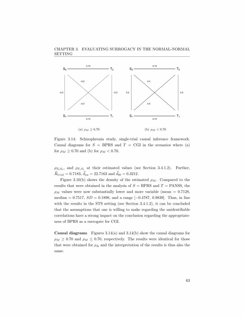
CHAPTER 3. EVALUATING SURROGACY IN THE NORMAL-NORMALSETTING
S0
S1
−0.2
T0
T1
−0.2
−0.2
0.73
0.74
−0.2
(a) ⇢M � 0.70
S0
S1
0.3
T0
T1
0.4
0.4
0.73
0.74
0.3
(b) ⇢M < 0.70
Figure 3.14: Schizophrenia study, single-trial causal inference framework.Causal diagrams for S = BPRS and T = CGI in the scenarios where (a)for ⇢M � 0.70 and (b) for ⇢M < 0.70.
⇢T0S0 , and ⇢T1S1 at their estimated values (see Section 3.4.1.2). Further,bRtrial = 0.7183, bdaa = 22.7163 and bdbb = 0.3212.
Figure 3.10(b) shows the density of the estimated ⇢M . Compared to theresults that were obtained in the analysis of S = BPRS and T = PANSS, the⇢M values were now substantially lower and more variable (mean = 0.7128,median = 0.7517, SD = 0.1898, and a range [�0.4787, 0.9839]. Thus, in linewith the results in the STS setting (see Section 3.4.1.2), it can be concludedthat the assumptions that one is willing to make regarding the unidentifiablecorrelations have a strong impact on the conclusion regarding the appropriate-ness of BPRS as a surrogate for CGI.
Causal diagrams Figures 3.14(a) and 3.14(b) show the causal diagrams for⇢M � 0.70 and ⇢M 0.70, respectively. The results were identical for thosethat were obtained for ⇢� and the interpretation of the results is thus also thesame.
63

CHAPTER 3. EVALUATING SURROGACY IN THE NORMAL-NORMALSETTING
Table 3.7: Schizophrenia study. Summary statistics for ⇢� and ⇢M in thesettings where the sampling variability in the estimation of ⇢T0S0 and ⇢T1S1 isnot accounted for (left) and is accounted for (right).
Sampling variability not accounted for Sampling variability accounted forS T Mean SD Range Mean SD Range
⇢� BPRS PANSS 0.9567 0.0366 [0.6200; 0.9935] 0.9566 0.0367 [0.6122; 0.9940]
BPRS CGI 0.7108 0.2214 [�0.9429; 0.9996] 0.7094 0.2209 [�0.9681; 0.9998]
S T Mean SD Range Mean SD Range⇢M BPRS PANSS 0.9577 0.0285 [0.7515; 0.9852] 0.9575 0.0286 [0.7554; 0.9863]
BPRS CGI 0.7145 0.1892 [�0.4708; 0.9850] 0.7133 0.1894 [�0.4845; 0.9877]
3.4.3 Accounting for the sampling variability in the es-
timation of ⇢S0T0 and ⇢S1T1
In the analyses detailed above, the sampling variability in the estimation of⇢S0T0 and ⇢S1T1 was not accounted for in the computation of ⇢� and ⇢M , i.e.,these correlations were fixed at their estimated values. To take the imprecisionin the estimation of ⇢S0T0 and ⇢S1T1 into account in the sensitivity analysis,these correlations can be sampled from a uniform distribution with [min, max]values equal to the upper and lower bounds of their corresponding CI95%.Thus, for each of the 21
4 matrices that are considered in the analyses, different⇢S0T0 and ⇢S1T1 values are sampled from these uniform distributions instead ofkeeping them fixed at their estimated values.
Table 3.7 shows the results. As can be seen, the effect of taking the im-precision in the estimation of ⇢S0T0 and ⇢S1T1 into account on the results wassmall and did not affect the substantive conclusions of the analyses in any way.
3.4.4 Conclusion
The analyses based on individual- and expected causal effects in both the single-and multiple-trial settings led to similar conclusions: the BPRS is an excellentsurrogate for the PANSS, whereas the appropriateness of the BPRS as a sur-rogate for the CGI could not be clearly established.
64

CHAPTER 3. EVALUATING SURROGACY IN THE NORMAL-NORMALSETTING
3.5 Discussion
In the current chapter, new metrics of surrogacy based on individual causaleffects in the STS and MTS were proposed. It was shown that the metrics ofsurrogacy based on individual and expected causal effects are related, but thecomplex nature of their relationship hindered the use of analytical techniquesto gain more insight in this relationship. One way to deal with this issue is tosimplify the problem by making additional assumptions. For example, when itcan be assumed that the potential outcomes for S and T are independent, itcan be heuristically shown that a surrogate that is successfully evaluated in themeta-analytic framework will typically also be appealing for proponents of thecausal inference framework (see Section 3.2.5). However, the latter assumptionis generally implausible. Indeed, it is natural to expect that the potentialoutcomes for S and T are correlated within the same patients, due to e.g.,genetic factors.
Alternatively, simulations can be used to evaluate the relationship betweenthe metrics of surrogacy that are based on individual and expected causal ef-fects under less restrictive assumptions. In the STS, the simulation resultsshowed that the relationship between the identifiable correlation � and theunidentifiable ⇢� is valid beyond the assumptions that were used to deriveLemma 1. The simulations also confirmed the consented view that, in general,a correlate (high ⇢S0T0 and ⇢S1T1) does not make a surrogate (Fleming andDeMets, 1996). In the MTS, the simulations showed that a surrogate that issuccessfully evaluated in the meta-analytic framework (i.e., high Rindiv andRtrial) will often also be appealing in a causal inference framework (i.e., high⇢M ) when it is reasonable to assume that all correlations between the poten-tial outcomes are positive. Importantly, the simulations also indicated that asurrogate that is successfully evaluated in the STS (large ⇢�) is not necessarilyan appropriate surrogate when evaluated in the MTS (low ⇢M ). Overall, theresults of the simulations showed that the extent to which the causal inferenceand meta-analytic surrogate evaluation paradigms lead to similar conclusionsregarding the appropriateness of the surrogate at hand is the result of a com-plex interplay between multiple factors, in particular (i) the setting that isused to assess surrogacy (i.e., the STS versus MTS), (ii) the parameter es-timates that are obtained for the identifiable quantities in ⇢� and ⇢M (e.g.,
65

CHAPTER 3. EVALUATING SURROGACY IN THE NORMAL-NORMALSETTING
the trial- and individual-level variance components), (iii) the assumptions thatare made regarding the correlations between the potential outcomes, and (iv)the assumptions that are made regarding the individual-level variance compon-ents (i.e., is homoscedasticity assumed or not). For example, the simulationsshowed that ⇢M is close to Rtrial when the trial-level variability componentsare ‘substantially larger’ than the individual-level variability components. Thisresult is insightful, but it does not allow for specifying a threshold for the ra-tio of the trial- and individual-level variance components that guarantees agood agreement between the meta-analytic and causal inference based metricsof surrogacy in a particular dataset. With respect to the latter issue, the Rpackage Surrogate provides a convenient tool. Indeed, this package allows forthe simultaneous examination of the combined impact of these different factorsthat affect agreement in a straightforward way.
In spite of being a powerful theoretical tool, the use of potential endpointsalso raises some major methodological challenges. For example, the develop-ments in the current chapter are predicated by the assumption that the po-tential outcomes are normally distributed endpoints. Even though the jointdistribution of the subvector (Tkj , Skj) is identifiable for k = {0, 1}, since(Tkj , Skj) ⇠ {(Tj , Sj) |Zj = k}, these marginal distributions do not fully de-termine the joint multivariate distribution of Y j , and, consequently, the nor-mality assumption previously postulated is not entirely verifiable. Notwith-standing these identifiability issues, the normal distribution has already beenused to model vectors of potential outcomes in this context. For example, Con-lon, Taylor and Elliott (2014) developed a Bayesian estimation strategy for theevaluation of surrogate endpoints assuming a multivariate normal distributionfor the vector of potential outcomes. In the next chapter, the focus will be onthe setting where both S and T are binary endpoints.
66

Chapter 4
Evaluating surrogacy in the
binary-binary setting based
on information theory and
causal inference
4.1 Introduction
As was detailed in the previous chapter, most surrogate evaluation methodsthat were developed within the causal inference framework (i) used individualcausal effects as the primary building blocks for the analysis (rather than ex-pected causal effects), and (ii) assumed that the data of a single clinical trialare available for analysis (rather than the data of multiple clinical trials). Inthe previous chapter, the focus was on the evaluation of surrogate endpoints inthe setting where both S and T are normally distributed variables. Here, thefocus will be on the setting where both S and T are binary endpoints.
In Section 4.2, the causal inference framework in the binary-binary singletrial setting (STS) is detailed. Based on this framework and information-theoretic concepts, new metrics of surrogacy are introduced in Sections 4.3–4.4. As was also the case in the continuous-continuous setting, a sensitivityanalysis will be used to deal with the identifiability issues of the metrics of
67

CHAPTER 4. EVALUATING SURROGACY IN THE BINARY-BINARYSETTING
interest. Finally, the methodology will be illustrated in a case study in Section4.5.
4.2 The causal inference framework
In this chapter, it will be assumed that data for both S and T are availablefrom a single clinical trial and that only two treatments are under evaluationin a parallel study design. Further, it will be assumed that both endpoints arebinary variables.
As was also the case in the normal-normal setting (see Chapter 3), Rubin’smodel for causal inference (Rubin, 1986) will be used. For simplicity, thefocus is temporarily on T alone. Under Rubin’s model for causal inference,each patient has two potential outcomes Y T = (T0, T1)
0, i.e., the outcomes foran individual had he or she received the experimental treatment (T1) or thecontrol treatment (T0). The bivariate distribution of Y T is characterized bythe parameters ⇡T
ij = P (T0 = i, T1 = j) with i, j = 0, 1 and it has marginals⇡Ti. =
Pj ⇡
Tij , ⇡T
.j =P
i ⇡Tij .
The so-called fundamental problem of causal inference states that only oneof T0 and T1 is observed and thus the distribution of Y T is often not identifiable(Holland, 1986). In particular, the association structure of the two potentialoutcomes, which is of primary interest in a surrogate evaluation context, cannotbe inferred from the data. Unlike the association structure between the po-tential outcomes, the marginal probabilities
�⇡T0·,⇡
T1·,⇡
T·0,⇡
T·1�0 are identifiable
under fairly general conditions. Indeed, if we denote by T the observed outcomefor a patient, then T = ZT1 + (1 � Z)T0 under SUTVA. Furthermore, if thetreatment allocation is made independently of the potential outcomes (Y T?Z),then ⇡T
1· = E (T |Z = 0) with ⇡T0· = 1�⇡T
1· and similarly ⇡T·1 = E (T |Z = 1) with
⇡T·0 = 1 � ⇡T
·1. Due to the random treatment allocation, the assumption of in-dependence Y T?Z can often be guaranteed in randomized clinical trials.
The marginal probabilities�⇡T0·,⇡
T1·,⇡
T·0,⇡
T·1�0 are not sufficient to identify
the entire bivariate distribution of the potential outcomes. Consequently, fur-ther assumptions regarding their association are required. To this end, letus consider the odds ratio ✓T = ⇡T
00 ⇡T11/⇡
T10 ⇡
T01. Using ✓T and the marginal
probabilities, the full bivariate distribution of Y T can be recovered (Plackett,
68

CHAPTER 4. EVALUATING SURROGACY IN THE BINARY-BINARYSETTING
1965)
⇡T11 =
8>><
>>:
1 +
�⇡T1· + ⇡T
·1�(✓T � 1)�WT
2 (✓T � 1)
if ✓T 6= 1,
⇡T1· ⇡
T·1 if ✓T = 1,
where WT =
q⇥1 +
�⇡T1· + ⇡T
·1�(✓T � 1)
⇤2+ 4✓T (1� ✓T )⇡T
1·⇡T·1. Further, the
individual causal effect of the treatment on T can be defined as �T = T1�T0,which follows a multinomial distribution with parameters ⇡�T
i = P (�T = i) =P
pq ⇡Tpq with i = �1, 0, 1 and the sum taken over all sub-indexes p, q satisfying
q � p = i. As was also the case for the distribution of Y T , the distribution of�T is not identifiable from the data without making untestable assumptionsregarding the association structure of the potential outcomes. Nonetheless,once ✓T is fixed, the distribution of �T becomes fully identifiable.
Let us now consider both endpoints S and T . In this setting, it is as-sumed that each patient has a four-dimensional vector of potential outcomesY = (T0, T1, S0, S1)
0. As before, the potential outcomes (S0, S1)0 can be used
to define the individual causal treatment effect on the surrogate �S and itsdistribution. The causal treatment effect on both endpoints is given by thevector � = (�T,�S)
0, and it follows the multinomial distribution given inTable 4.1.
Table 4.1: Distribution of � = (�T,�S)0.
�S
-1 0 1
�T
-1 ⇡��1�1 ⇡�
�10 ⇡��11 ⇡�T
�1
0 ⇡�0�1 ⇡�
00 ⇡�01 ⇡�T
0
1 ⇡�1�1 ⇡�
10 ⇡�11 ⇡�T
1
⇡�S�1 ⇡�S
0 ⇡�S1 1
69
CHAPTER 4. EVALUATING SURROGACY IN THE BINARY-BINARYSETTING
4.3 Individual causal association
A new metric to quantify surrogacy in the binary-binary setting is proposed inSection 4.3.2. This metric is based on information-theoretic concepts that areintroduced in the next section.
4.3.1 Information theory
The concept of entropy, which can be interpreted as a measure of the ran-domness or the uncertainty that is associated with a random variable, is fun-damental in information theory (Shannon, 1948). If Y is a discrete randomvariable which can take values {y1, y2, . . . , ym} with a probability functionP (Y = yi) = pi, then the entropy of Y is defined as
H(Y ) = �EY [logP (Y )] = �
X
i
pi log pi.
Similarly, the joint and conditional entropies of two discrete random variablesX and Y are defined as
H(X,Y ) = �EX,Y [logP (X,Y )],
andH(Y |X) = �EX [EY (logP (Y |X))],
respectively, with P (X,Y ) and P (Y |X) denoting the joint and conditionalprobability functions, respectively. Entropy is always non-negative and satis-fies H (Y |X) H(Y ) for any pair of random variables (X,Y ), with equalityholding under independence. Basically, the previous inequality states that, onaverage, the uncertainty with respect to Y can only decrease when additionalinformation (i.e., X) becomes available. Furthermore, entropy is invariant un-der a bijective transformation.
The amount of uncertainty in Y that is expected to be removed when thevalue of X becomes known, is quantified by the so-called mutual information
I (X,Y ) = H (Y )�H (Y |X) .
Mutual information is always non-negative, is zero if and only if X and Y areindependent, is symmetric and invariant under bijective transformations of X
70

CHAPTER 4. EVALUATING SURROGACY IN THE BINARY-BINARYSETTING
and Y , and I(X,X) = H(X). Further, mutual information approaches infinityas the distribution of (X,Y ) approaches a singular distribution, i.e., I(X,Y ) islarge when there is an approximate functional relationship between X and Y
(Joe, 1989). It follows from the definitions of entropy and mutual informationthat
I(X,Y ) = H(X) +H(Y )�H(X,Y ) =
X
X,Y
P (X,Y ) log
✓P (X,Y )
P (X)P (Y )
◆,
where P (X,Y ), P (X), and P (Y ) denote the joint and marginal probabilityfunctions of X and Y , respectively. Based on mutual information, Joe (1989)introduced the informational coefficient of correlation, which is given by
⇢I(X,Y ) =
p1� e�2I(X,Y ). (4.1)
The informational coefficient of correlation is always in the unit interval, isinvariant under bijective transformations, and is equal to zero if and only if Xand Y are independent. For continuous variables, ⇢I approaches 1 if and onlyif there exists an approximate functional relationship among X and Y (Joe,1989).
4.3.2 Definition of R2H
For continuous and normally distributed endpoints, the individual causal as-sociation can be defined using the correlation between the individual causaltreatment effects on S and T , i.e. ⇢� = corr (�T,�S) (for details see Section3.2.1). In a more general setting, irrespective of the distributions of S andT , one would intuitively expect that if S is a good surrogate for T then �S
should convey a substantial amount of information regarding �T . The mutualinformation between both individual causal treatment effects (i.e., I(�T,�S))quantifies the amount of uncertainty in �T that is expected to be removedwhen the value of �S becomes known, and it can thus be argued that this isa useful metric to evaluate the appropriateness of a candidate surrogate.
For continuous and normally distributed outcomes, ⇢I (�T,�S) = |⇢�|.However, the informational coefficient of correlation (4.1) is not appropriatein the current setting. Indeed, when applied to discrete random variables,⇢I (�T,�S) does not equal one when there is a functional relationship betweenboth variables. To this end, and in line with Joe (1989), in the binary-binary
71

CHAPTER 4. EVALUATING SURROGACY IN THE BINARY-BINARYSETTING
scenario it is proposed to quantify ICA, i.e., the association between �T and�S, using the following transformation of the mutual information
R2H(�T,�S) =
I(�T,�S)
min [H(�T ), H(�S)], (4.2)
where the mutual information is given by
I(�T,�S) =
1X
i,j=�1
⇡�ij log
⇡�ij
⇡�Ti ⇡�S
j
!,
and the entropies of the individual causal treatment effects by
H(�T ) =�
1X
i=�1
⇡�Ti log(⇡�T
i ),
H(�S) =�
1X
j=�1
⇡�Sj log(⇡�S
j ).
Along the lines discussed in Joe (1989), it can be shown that R2H(�T,�S)
is invariant under one-to-one transformations. Further, R2H(�T,�S) always
lies in the unit interval, where it takes value zero when �T and �S are inde-pendent and value one when there is a nontrivial transformation such thatP [�T = (�S)] = 1. In the next section, R2
H(�T,�S) is compared withother metrics of surrogacy that were proposed in the literature.
4.3.3 Relationship between the individual causal associ-
ation and other metrics of surrogacy
Frangakis and Rubin (2002) introduced a principal stratification approach toevaluate surrogacy and suggested that the appropriateness of a candidate sur-rogate should be assessed based on the size of its associative effect (AE) relativeto its dissociative effect (DE). An effect is associative when the causal treat-ment effect on T is reflected on the causal treatment effect on S, otherwiseit is dissociative. A good S is expected to have a large AE, i.e., the causaltreatment effect on S should be strongly associated with the causal treatmenteffect on T . Similarly, a good S is expected to have a small DE, i.e., the causaltreatment effect on T should be small when the causal treatment effect on S iszero (Li, Taylor and Elliott, 2010; Elliott, Li and Taylor, 2013).
72

CHAPTER 4. EVALUATING SURROGACY IN THE BINARY-BINARYSETTING
Table 4.2: R2H versus other metrics of surrogacy
Case Causal effects AE DE CET AP DP R2H
1 �T = �S ⇡�11 � ⇡�
�1�1 0 ⇡�11 � ⇡�
�1�1 1 0 1
2 �T = ��S ⇡�1�1 � ⇡�
�11 0 ⇡�1�1 � ⇡�
�11 1 0 1
3 �T = �S2 ⇡�11 � ⇡�
1�1 0 ⇡�11 � ⇡�
1�1 1 0 1
4 �T = �S2� 1 0 �⇡�
�10 �⇡��10 0 1 1
5 �T?�S�1� ⇡�S
0
�CTE ⇡�S
0 CTE ⇡�T1 � ⇡�T
�1 1� ⇡�S0 ⇡�S
0 0
Using the notation in Table 4.1, Elliott, Li and Taylor (2013) defined AE asAE =
�⇡�11 � ⇡�
�11
�+
�⇡�1�1 � ⇡�
�1�1
�, i.e., AE is the net treatment effect on
patients whose surrogate was responsive to the treatment. Furthermore, DE =
⇡�10 � ⇡�
�10, i.e., DE is the net treatment effect on patients whose surrogatewas not responsive to the treatment. Finally, the causal treatment effect on thetrue endpoint is defined as CET = ⇡�T
1 � ⇡�T�1 , i.e., the net treatment effect
corresponding to the fraction of patients who benefited from the treatmentminus those who were harmed by the treatment. Because AE and DE areconstrained to sum to CET , Taylor, Wang and Thıébaut (2005) proposed to usethe so-called associative (AP = AC/CET ) and dissociative (DP = DE/CET )proportions, respectively. A good surrogate is then expected to have a largeAP and a small DP .
Let us now compare R2H (see expression (4.2)) with these other metrics of
surrogacy across a number of theoretical settings. A summary of the results isgiven in Table 4.2 and a formal deduction of the expressions in the table canbe found in the Appendix Section B.
In the first four settings there is a deterministic relationship between �T
and �S. For example, in the first row P (�T = �S) = 1 and, therefore, know-ing the impact of Z on S allows predicting the impact of Z on T without error.This is correctly captured by R2
H , indicating that the uncertainty regarding �T
is fully reduced when �S becomes known. Interestingly, AP and DP indicatethat the first three cases in Table 4.2 are perfect surrogates (i.e., AP = 1 andDP = 0), whereas the fourth case is not (i.e., AP = 0 and DP = 1). Giventhat in all four cases �T can be predicted with perfect accuracy based on �S,these different conclusions in the assessment of cases 1–3 and case 4 seem inco-
73

CHAPTER 4. EVALUATING SURROGACY IN THE BINARY-BINARYSETTING
herent. Indeed, in spite of the striking similarity between cases 3 (�T = �S2)and 4 (�T = �S2
� 1), AP and DP provide an entirely different assessmentof surrogacy.
In case 5, �T and �S are independent, i.e., the individual causal treatmenteffect on S conveys no information regarding the individual causal treatmenteffect on T . This is correctly captured by R2
H = 0, i.e., knowing the individualcausal treatment effect on S does not reduce the uncertainty regarding theindividual causal treatment effect on T . However, if ⇡�S
0 is small then AP ⇡ 1
and DP ⇡ 0, and thus the appropriateness of S would be supported. In fact,AP and DP can take all possible values in this setting depending on the valueof ⇡�S
0 . These results seem to indicate that, at least in some scenarios, R2H
may offer a more coherent assessment of surrogacy than AP and DP .Frangakis and Rubin (2002) also introduced an alternative definition of sur-
rogacy, the so-called ‘principal surrogate’. A surrogate is said to be a principalsurrogate for the effect of Z on T if for all patients j, P (T1|S1 = S0 = j) =
P (T0|S1 = S0 = j). If T is binary then the definition of a principal surrogateis equivalent to E(T1 � T0|S1 = S0) = 0 or, using the notation in Table 4.1,E(�T |�S = 0) = 0 (VanderWeele, 2013). VanderWeele (2008) referred to thiscondition as no principal strata direct effects, whereas Gilbert and Hudgens(2008) called it the property of causal necessity (see also Section 3.2.2). Noticethat E(�T |�S = 0) = (⇡�
10 � ⇡��10)/⇡
�S0 = DE/⇡�S
0 when both endpointsare binary and therefore principal surrogacy (causal necessity) is equivalent toDE = 0 (or, in terms of the associative and dissociative proportions, equivalentto AP = 1 and DP = 0). As case 4 in Table 4.2 illustrates, a surrogate thatcompletely predicts the individual causal treatment effect on T may not satisfythe property of causal necessity, i.e., it may not be a principal surrogate. Inaddition, as case 5 in Table 4.2 shows, a surrogate for which �T and �S areindependent may still satisfy the property of causal necessity and consequentlybe a valid principal surrogate.
4.3.4 Identifiability issues
Causal inference models are conceptually attractive tools to evaluate surrogateendpoints, but their practical use is challenging. Indeed, all the metrics ofsurrogacy that were discussed above are based on the distribution of the vector
74

CHAPTER 4. EVALUATING SURROGACY IN THE BINARY-BINARYSETTING
of individual causal treatment effects � (see Table 4.1), but this distributionis not identifiable from the data and consequently these measures cannot bedirectly estimated (a similar problem occurred in the setting where both S andT were normally distributed endpoints, see Section 3.2.4).
These identifiability problems are often tackled by defining identifiabil-ity conditions that allow for estimating the distributions of interest. Onesuch condition is the so-called monotonicity assumption. Under monotonicity,P (T0 T1) = P (S0 S1) = 1 and thus ⇡T
10 = ⇡S10 = 0. Identifiability condi-
tions are frequently combined with additional modelling assumptions in orderto estimate the parameters of interest. For example, Li, Taylor and Elliott(2010) estimated the associative and dissociative proportions using a Bayesianmodelling approach. These authors treated the unobserved potential outcomesas missing data and applied imputation techniques. Identifiability was achievedunder the assumption of monotonicity by selecting appropriate prior distribu-tions for the unidentifiable parameters. Elliott, Li and Taylor (2013) implemen-ted a similar Bayesian approach to estimate the associative proportion underdifferent monotonicity assumptions and missing data generating mechanisms.
Here, the identifiability problem is approached from a different perspect-ive in the same spirit as was done in the normal-normal setting (see Sec-tion 3.2.4). In particular, a two-step procedure based on the distribution ofthe vector of potential outcomes Y was used. The distribution of Y has aparameter space given by � =
�⇡ 2 [0, 1]16 : 1⇡ = 1
, where ⇡ = (⇡ijpq),
⇡ijpq = P (T0 = i, T1 = j, S0 = p, S1 = q) and i, j, p, q = 0/1. In the first step,the subspace �D ⇢ � that is compatible with the data at hand is geometricallycharacterized. Next, the behaviour of R2
H on �D can be studied. Given thatR2
H is unidentifiable, this approach is not aimed at estimating its ‘true value’.The proposed methodology can better be described as a sensitivity analysis.In fact, each point in �D can be conceptualized as a ‘reality’ that is compatiblewith the data. Therefore, the behaviour of R2
H on �D describes the appropri-ateness of the surrogate across all scenarios that are compatible with the data.In the next sections, this approach is described in more detail.
75

CHAPTER 4. EVALUATING SURROGACY IN THE BINARY-BINARYSETTING
4.3.4.1 Step 1: Geometrically characterizing �D
The data at hand impose some restrictions on the parameters ⇡ijpq that de-scribe the distribution of the potential outcomes (see also Elliott, Li and Taylor,2013; Li, Taylor and Elliott, 2010). Basically, the data allow for the identific-ation of three probabilities P (T = t, S = s|Z) within each treatment group.Thus, in total there are 16 parameters characterizing the distribution of Y andthese parameters are subjected to 7 restrictions, implying that 9 parametersare allowed to vary freely and, consequently, are not identifiable from the data.The set of restrictions can be written as
⇡1·1· = P (T = 1, S = 1|Z = 0), ⇡·1·1 = P (T = 1, S = 1|Z = 1),
⇡1·0· = P (T = 1, S = 0|Z = 0), ⇡·1·0 = P (T = 1, S = 0|Z = 1), (4.3)
⇡0·1· = P (T = 0, S = 1|Z = 0), ⇡·0·1 = P (T = 0, S = 1|Z = 1),
⇡···· = 1,
with the points in the sub-indexes indicating sums over thosespecific sub-indexes. Further, if one defines the vector b
0=
(1,⇡1·1·,⇡1·0·,⇡·1·1,⇡·1·0,⇡0·1·,⇡·0·1), and the matrix
A =
0
BBBBBBBBBBBBB@
1 1 1 1 1 1 1 1 1 1 1 1 1 1 1 1
0 0 0 0 0 0 1 0 1 0 1 1 0 0 0 0
0 0 0 0 0 1 0 1 0 1 0 0 0 0 0 1
0 0 0 0 1 0 0 0 0 1 0 1 0 0 1 0
0 1 0 0 0 0 0 0 1 0 0 0 1 0 0 1
0 0 1 0 0 0 0 0 0 0 0 0 1 1 1 0
0 0 0 1 0 0 0 1 0 0 1 0 0 1 0 0
1
CCCCCCCCCCCCCA
,
then all the restrictions given in (4.3) can be written as a system of linearequations
A⇡ = b, (4.4)
where the vector of parameters ⇡ is ordered as in Table 4.3. The hyperplanegiven in expression (4.4) geometrically characterizes the subspace of � that iscompatible with the data at hand, i.e., �D = {⇡ 2 � : A⇡ = b}. The matrixA has rank 7 and it can be partitioned as A = (Ar|Af ), where Af denotesthe submatrix given by the last 9 columns of A and Ar is a full column rank
76

CHAPTER 4. EVALUATING SURROGACY IN THE BINARY-BINARYSETTING
matrix. Similarly, the vector ⇡ can be partitioned as ⇡0=
⇣⇡
0r|⇡
0f
⌘with ⇡f
the subvector given by the last 9 components of ⇡. Using these partitions thesystem of linear equations (4.4) can be rewritten as Ar⇡r + Af⇡f = b.
Table 4.3: Distribution of Y
⇡ T0 T1 S0 S1
⇡0000 0 0 0 0
⇡0100 0 1 0 0
⇡0010 0 0 1 0
⇡0001 0 0 0 1⇡0101 0 1 0 1
⇡1000 1 0 0 0
⇡1010 1 0 1 0⇡1001 1 0 0 1
⇡1110 1 1 1 0
⇡1101 1 1 0 1
⇡1011 1 0 1 1⇡1111 1 1 1 1
⇡0110 0 1 1 0
⇡0011 0 0 1 1⇡0111 0 1 1 1
⇡1100 1 1 0 0
As stated above, the behaviour of R2H on �D can be evaluated to examine
the appropriateness of the surrogate across all ‘realities’ that are compatiblewith the data. Studying the behaviour of a function on a region of an Euclideanspace is a deterministic problem. However, the use of graphical or analyticaltechniques in this scenario is rather cumbersome due to the complex way inwhich R2
H depends on ⇡ and the high dimensionality of the latter. In the nextsection, these issues are tackled using a Monte Carlo approach. Monte Carlomethods are often used for obtaining numerical solutions for problems that aretoo complicated to solve analytically.
77

CHAPTER 4. EVALUATING SURROGACY IN THE BINARY-BINARYSETTING
4.3.4.2 Step 2: Assessing R2H
To study the behaviour of R2H on �D, a Monte Carlo approach will be followed.
Basically, points will be uniformly sampled on �D and the value of R2H will
be calculated for these sampled values. The use of a uniform distributionto explore �D guarantees that all regions on the hyperplane have the samechance of being covered by the sampling scheme. The general behaviour of R2
H
can subsequently be examined using descriptive statistics or simple graphicaltechniques like e.g., histograms.
The following algorithm can be used to sample points on �D:
1. Select a grid of values G = {g1, g2, ..., gK} in (0, 1).2. From k = 1 until K do:
(a) Using the Randfixedsum algorithm (Emberson, Stafford and Davis,2010; Stafford, 2006), generate the 9 components of ⇡f uniformallyin the hyperplane 10
⇡f = gi.(b) Calculate ⇡r = A�1
r (b� Af⇡f ) and ⇡0=
⇣⇡
0r|⇡
0f
⌘.
(c) Repeat steps 2a and 2b M times.
3. From these K ⇥M ⇡ vectors, select those with all components positive(the valid vectors ⇡ > 0).
The vectors ⇡km can be used to obtain the distribution of the vector of theindividual causal effects �, given in Table 4.1, as
⇡��1�1 = ⇡1010, ⇡�
0�1 = ⇡0010 + ⇡1110,⇡�1�1 = ⇡0110, ⇡�
�10 = ⇡1000 + ⇡1011,⇡��11 = ⇡1001, ⇡�
01 = ⇡0001 + ⇡1101,
⇡�11 = ⇡0101, ⇡�
10 = ⇡0100 + ⇡0111,⇡�00 = ⇡0000 + ⇡0011 + ⇡1100 + ⇡1111,
(4.5)
and ⇡�11 = 1�⇡�
�1�1�⇡�0�1�⇡
�1�1�⇡
��10�⇡
�00�⇡
�10�⇡
��11�⇡
�01. Based on these
values, the individual causal association R2H can be calculated using expression
(4.2). Note that this algorithm implicitly assumes that none of the componentsof ⇡ lies on the boundary of the parameter space, but it can easily be adaptedto explore regions in which some components ⇡ are zero (e.g., regions wheremonotonicity holds; details are provided in Appendix Section C).
78

CHAPTER 4. EVALUATING SURROGACY IN THE BINARY-BINARYSETTING
4.3.4.3 Remarks on identifiability conditions
The vector ⇡ characterizes the distribution of Y and its components are themost fundamental parameters describing the behaviour of the potential out-comes. Any other set of parameters, like the odds ratios ✓T and ✓S (thatquantify the association between the potential outcomes for S and T ), can bewritten as a function of the components of ⇡. As a consequence, the set oflinear equations given in expression (4.4) also impose restrictions on all otherparameters obtained from ⇡, including ✓T and ✓S . However, these derivedparameters are often complex nonlinear functions of the components of ⇡ and,consequently, the constrains imposed on them by (expression 4.4) can be rathercomplex as well.
Arbitrary assumptions for the association between the potential outcomeslike e.g., independence (i.e., ✓T = 1) or monotonicity (i.e., ✓T = 1) may beincompatible with expression (4.4) and lead to invalid conclusions. To exem-plify this issue, consider the setting where monotonicity holds for S and T , i.e.,⇡1000 = ⇡1010 = ⇡1001 = ⇡1011 = ⇡0010 = ⇡1110 = ⇡0110 = 0. These equalitieshave verifiable implications for the identifiable marginals in b. In fact, it canbe easily shown that if monotonicity holds then
⇡1·1· ⇡·1·1, ⇡·0·0 ⇡0·0·,
⇡0·1· ⇡·0·1 + ⇡·1·1, ⇡1·0· ⇡·1·1 + ⇡·1·0,
⇡·1·0 ⇡0·0· + ⇡1·0·, ⇡·0·1 ⇡0·0· + ⇡0·1·.
For example, the vector b = (1, 0.30, 0.35, 0.20, 0.10, 0.05, 0.30)0 does not satisfy
the aforementioned necessary conditions. Thus, it is incompatible with themonotonicity assumption. Clearly, assuming monotonicity in such a settingmay be misleading.
4.4 The surrogate predictive function
4.4.1 Definition
In Section 4.3, it was shown that R2H equals zero when �T and �S are inde-
pendent and that R2H equals one when there is a non-trivial transformation
such that P [�T = (�S)] = 1 (i.e., there exists a deterministic relationship
79

CHAPTER 4. EVALUATING SURROGACY IN THE BINARY-BINARYSETTING
�T = (�S)). The R2H (�T,�S) metric thus provides a general quantifica-
tion of the surrogate predictive value, but it does not provide any informationregarding the specific form of the prediction function .
To explore this issue, let us now consider a general prediction function : {�1, 0, 1} ! {�1, 0, 1}. The predictive value of can be assessed usingthe expression
P [�T = (�S)] =1X
i=�1
P (�T = i, (�S) = i) , (4.6)
=
1X
i=�1
X
j2 �1(i)
P (�T = i,�S = j) ,
=
1X
i=�1
X
j2 �1(i)
P (�T = i|�S = j)P (�S = j) ,
where �1(i) : {j 2 {�1, 0, 1} : (j) = i}. The probabilities P (�S = j) do
not involve T and they can be considered an intrinsic characteristic of thepair (S,Z). On the other hand, the function r : {�1, 0, 1}2 ! [0, 1] givenby r(i, j) = P (�T = i|�S = j) fully captures the relationship between theindividual causal treatment effects on S and T in (4.6).
We shall call r (�T = i,�S = j) the surrogate predictive function (SPF),i.e., the function that allows us to determine what the most likely outcomeof �T will be for a given value of �S. The SPF allows for the evaluation ofsome important scientific questions that cannot be explicitly answered usingR2
H(�T,�S). For example, r(�1, 1) quantifies the conditional probability thatZ has a negative impact on T given that Z has a beneficial impact on S
(i.e., the probability that the surrogate will produce a false positive result).Similarly, r(1,�1) quantifies the conditional probability that Z has a beneficialimpact on T given that Z has a negative impact on S (i.e., the probabilitythat the surrogate will produce a false negative result). It can be argued thatr(�1, 1) = r(1,�1) ⇡ 0 is a desirable property for a ‘good’ S.
80

CHAPTER 4. EVALUATING SURROGACY IN THE BINARY-BINARYSETTING
4.4.2 Relationship between the surrogate predictive func-
tion and other metrics of surrogacy
The SPF is related to other concepts that were previously introduced in theliterature. For example, the SPF is intrinsically related to the concept of causalnecessity (see Sections 3.2.2 and 4.3.3) that was proposed by Frangakis andRubin (2002). Indeed, causal necessity can be re-stated as r(0, 0) = 1. Anotherinteresting conceptual setting arises when P [�T = �S] = 1, i.e., the individualcausal treatment effects on S and T are identical. Lemma 2 characterizes theprevious scenario using the SPF (the proof is straightforward).
Lemma 2. Let T and S denote a binary true and surrogate endpoint,respectively. Under the causal inference model introduced in Section 4.2,P [�T = �S] = 1 if and only if r(i, j) = 0 for all i 6= j.
Furthermore, there is a close relationship between the SPF and the bestprediction function associated with the distribution of �. To illustratethis, let us first define the best prediction function as the function b =
argmax P [�T = (�S)]. Lemma 3 describes the relationship between theSPF and the best prediction function (the proof is provided in Section D of theAppendix).
Lemma 3. Let T and S denote a binary true and surrogate endpoint respect-ively. Further, let b : {�1, 0, 1} ! {�1, 0, 1} be the function defined as
b(j) = arg max
ir(i, j) = arg max
iP (�T = i|�S = j)
If the argument function in the previous equation returns more than one value,then any of them can be chosen arbitrarily to define b(j) and thus b will notbe unique. The function b is the best prediction function associated with thedistribution of �.
4.4.3 Assessing the SPF
As was also the case for R2H , the SPF is not identifiable from the data and it
can thus not be directly estimated. The sensitivity-based approach detailed inSection 4.3.4 can again be used to deal with these identifiability issues. Briefly,in this approach (i) the subspace �D ⇢ � that is compatible with the data at
81

CHAPTER 4. EVALUATING SURROGACY IN THE BINARY-BINARYSETTING
hand is first characterized, and (ii) the behaviour of the SPF on �D is studied.The obtained vectors ⇡km are subsequently used to compute the vectors of theindividual causal effects � (given in Table 4.1) using the expressions given in(4.5). Based on these values, the SPF can be computed as
r(i, j) =⇡�ij
⇡�Sj
, (4.7)
with ⇡�Sj =
Pj ⇡
�ij . Again, this approach is not aimed at estimating the ‘true’
SPF (which is unidentifiable). Instead, it can be conceptualized as a sensitivityanalysis where each point in �D is a ‘reality’ that is compatible with ours (i.e.,the identifiable marginal probabilities in the dataset at hand).
4.5 Case study: a clinical trial in schizophrenia
In Section 2.1.1, the data of five clinical trials in schizophrenia were detailed.Here, a subset of those data are analysed. In particular, the data of one of theclinical trials (i.e., the INT-2 trial) was selected for analysis (recall that R2
H
and SPF are STS-based metrics of surrogacy). This trial included a total of454 patients who were all treated for eight weeks. The control treatment (doseof 10 mg. of haloperidol) and the experimental treatment (dose of 8 mg. ofrisperidone) were given to 225 and 229 patients, respectively.
In the analyses below, it will be examined (i) whether clinically relevantchange in the BPRS score is a good surrogate for clinically relevant changein the PANSS score, and (ii) whether clinically relevant change in the BPRSscore is a good surrogate for clinically relevant change in the CGI score. Tables4.4 and 4.5 summarize the data. To simplify the exposition, the names ofthe endpoints (i.e., BPRS, PANSS and CGI) will be used to refer to clinicallyrelevant change in the scores for each scale.
The analyses detailed below are conducted using the R package Surrogate.In the current section, only a summary of the main results is given and no refer-ence to the software is made. A more comprehensive analysis and step-by-stepinstructions on how the results can be obtained using the Surrogate package isavailable in the online Appendix Chapter 2. The online appendix can be down-loaded at https://dl.dropboxusercontent.com/u/8416806/PhD_Appendix.pdf.
82

CHAPTER 4. EVALUATING SURROGACY IN THE BINARY-BINARYSETTING
Table 4.4: Schizophrenia study, binary-binary setting. Cross-tabulation of theBPRS (S) versus PANSS (T ) outcomes in the control (left) and experimental(right) treatment groups.
Control Experimental
T T
0 1 0 1
S0 105 12
S0 94 7
1 12 94 1 11 116
Table 4.5: Schizophrenia study, binary-binary setting. Cross-tabulation of theBPRS (S) versus CGI (T ) outcomes in the control (left) and experimental(right) treatment groups.
Control Experimental
T T
0 1 0 1
S0 49 68
S0 35 66
1 102 4 1 119 8
83

CHAPTER 4. EVALUATING SURROGACY IN THE BINARY-BINARYSETTING
0.2 0.3 0.4 0.5 0.6 0.7
01
23
45
6
RH2
Density
Figure 4.1: Schizophrenia study, binary-binary setting, S = BPRS and T =PANSS. Density of R2
H .
4.5.1 The BPRS as a surrogate for the PANSS
4.5.1.1 The individual causal association
The analysis was conducted using the sensitivity-based approach that was de-tailed in Section 4.3.4, fixing the marginal probabilities to their observed values(b⇡1·1· = 0.4215, b⇡0·1· = 0.0538, b⇡1·0· = 0.0538, b⇡·1·1 = 0.5088, b⇡·1·0 = 0.0307,and b⇡·0·1 = 0.0482) and using M = 10, 000 runs of the algorithm.
The density of R2H is shown in Figure 4.1. It was obtained that bR2
H mean= 0.5280, median = 0.5475, and SD = 0.0964. The results thus indicated thatthe individual causal treatment effect on the PANSS (i.e., �T ) can typically bepredicted with relatively low accuracy based on the individual causal treatmenteffect on the BPRS (i.e., �S).
Causal diagrams Figure 4.1 shows the density of R2H based on all vectors ⇡
that are compatible with the data at hand. These values ranged between 0.2352
84

CHAPTER 4. EVALUATING SURROGACY IN THE BINARY-BINARYSETTING
S0
S1
0.06
T0
T1
0.06
0.08
0.51
0.6
0.06
(a) R2H � 0.50
S0
S1
0.21
T0
T1
0.21
0.24
0.51
0.6
0.21
(b) R2H 0.50
Figure 4.2: Schizophrenia study, binary-binary setting. Causal diagrams forS = BPRS and T = PANSS in the scenarios where (a) R2
H � 0.50 and (b)R2
H 0.50.
and 0.6951, indicating that the unverifiable assumptions had a relatively strongimpact on R2
H . Based on the data alone, one cannot discriminate between thescenarios in which relatively large values of R2
H received more support andother scenarios in which smaller values of R2
H received more support.However, in some situations, expert knowledge may be available to evaluate
the plausibility of the different scenarios. In this context, it can be interestingto consider a subgroup of the results for closer inspection. Similarly to whatwas done in Chapter 3, causal diagrams that depict the median informationalcoefficients of correlation between the potential outcomes for a range of R2
H
values can be useful in this context.By means of illustration, Figures 4.2(a) and 4.2(b) show causal diagrams
that are compatible with R2H � 0.50 and R2
H 0.50. In these diagrams, thetwo horizontal lines depict the identifiable informational coefficients of associ-ation between S and T in the two treatment conditions, i.e., br2h(S0, T0) = 0.51
and br2h(S1, T1) = 0.60. Essentially, these coefficients quantify the strengthof the association between S and T in both treatment groups. The four non-horizontal lines depict the medians of the unidentified informational coefficientsof association between the counterfactuals. In the first causal diagram (for
85

CHAPTER 4. EVALUATING SURROGACY IN THE BINARY-BINARYSETTING
R2H � 0.50), the median informational association between the potential out-
comes for S and T are negligible, i.e., br2h(S0, S1) = br2h(T0, T1) = 0.06. Thismeans that a patient’s outcome on the BPRS/PANSS in the active controlcondition (S0/T0) essentially conveys no information on the patient’s outcomeon the BPRS/PANSS in the experimental treatment condition (S1/T1). Giventhat the treatments under study are similar and S0, S1 (and also T0, T1)are repeated measurements in the same patient, this independence does notappear to be biologically plausible. Further, the other median informationalassociations br2h(S0, T1) = 0.06 and br2h(S1, T0) = 0.08 are also low. Since theBPRS is a sub-scale of the more complex PANSS scale, one would also ex-pect a stronger level of association between these potential outcomes. In thesecond causal diagram (for R2
H 0.50), the median informational associationsbetween the potential outcomes are no longer close to zero. Indeed, the medianbr2h(S0, S1) = br2h(T0, T1) = br2h(S0, T1) = 0.21 and br2h(S1, T0) = 0.24. As wasdiscussed in the previous paragraph, this pattern of association between thepotential outcomes seems to be more compatible with expert knowledge.
Clearly, there will always be subjectivity involved in this type of qualitat-ive analysis. Nonetheless, expert opinion may provide useful information tointerpret the previous diagrams and evaluate their plausibility.
4.5.1.2 The Surrogate Predictive Function
Figure 4.3 shows the results of the SPF analyses. The bottom left figure inthe plot suggests that the probability of a false positive result is rather small,with mean r(�1, 1) = 0.0443. Further, the level of uncertainty with respect tothe true r(�1, 1) is also small with the range r(�1, 1) equal to [0.0007; 0.2324].The top right figure suggests that the probability of a false negative result issmall as well, with mean r(1,�1) = 0.0483, but now the range of the r(1,�1)
values is much wider [0.0001; 0.6067] indicating that there is a substantial levelof uncertainty with respect to the true r(1,�1). Further, the top left figureindicates that a negative individual causal treatment effect on the BPRS typ-ically leads to the prediction that the individual causal treatment effect on thePANSS is negative as well, with r(�1,�1) = 0.7484. Note however that thereis again a large level of uncertainty, with r(�1,�1) range [0.0585; 0.9717].
The results shown in the center figure offer some support for causal necessity
86
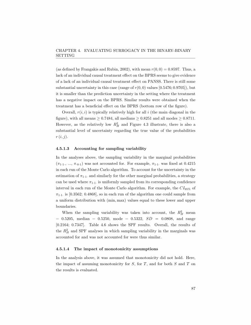
CHAPTER 4. EVALUATING SURROGACY IN THE BINARY-BINARYSETTING
(as defined by Frangakis and Rubin, 2002), with mean r(0, 0) = 0.8597. Thus, alack of an individual causal treatment effect on the BPRS seems to give evidenceof a lack of an individual causal treatment effect on PANSS. There is still somesubstantial uncertainty in this case (range of r(0, 0) values [0.5476; 0.9705]), butit is smaller than the prediction uncertainty in the setting where the treatmenthas a negative impact on the BPRS. Similar results were obtained when thetreatment has a beneficial effect on the BPRS (bottom row of the figure).
Overall, r(i, i) is typically relatively high for all i (the main diagonal in thefigure), with all means � 0.7484, all medians � 0.8251 and all modes � 0.8711.However, as the relatively low R2
H and Figure 4.3 illustrate, there is also asubstantial level of uncertainty regarding the true value of the probabilitiesr (i, j).
4.5.1.3 Accounting for sampling variability
In the analyses above, the sampling variability in the marginal probabilities(⇡1·1·, ..., ⇡·0·1) was not accounted for. For example, ⇡1·1· was fixed at 0.4215
in each run of the Monte Carlo algorithm. To account for the uncertainty in theestimation of ⇡1·1· and similarly for the other marginal probabilities, a strategycan be used where ⇡1·1· is uniformly sampled from its corresponding confidenceinterval in each run of the Monte Carlo algorithm. For example, the CI95% of⇡1·1· is [0.3562; 0.4868], so in each run of the algorithm one could sample froma uniform distribution with (min,max) values equal to these lower and upperboundaries.
When the sampling variability was taken into account, the R2H mean
= 0.5205, median = 0.5250, mode = 0.5322, SD = 0.0808, and range[0.2164; 0.7347]. Table 4.6 shows the SPF results. Overall, the results ofthe R2
H and SPF analyses in which sampling variability in the marginals wasaccounted for and was not accounted for were thus similar.
4.5.1.4 The impact of monotonicity assumptions
In the analysis above, it was assumed that monotonicity did not hold. Here,the impact of assuming monotonicity for S, for T , and for both S and T onthe results is evaluated.
87
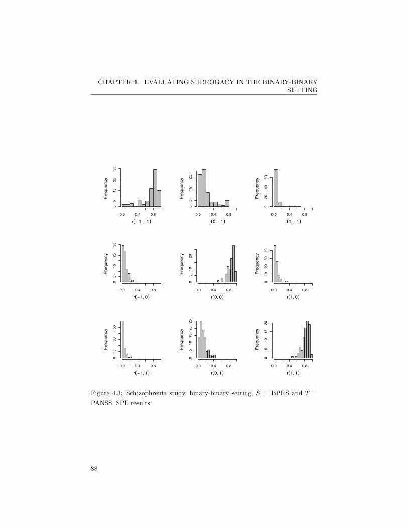
CHAPTER 4. EVALUATING SURROGACY IN THE BINARY-BINARYSETTING
r(−1, −1)
Frequency
0.0 0.4 0.8
05
1525
35
r(0, −1)
Frequency
0.0 0.4 0.8
05
1525
r(1, −1)
Frequency
0.0 0.4 0.8
020
4060
r(−1, 0)
Frequency
0.0 0.4 0.8
05
1525
35
r(0, 0)
Frequency
0.0 0.4 0.8
05
1020
r(1, 0)
Frequency
0.0 0.4 0.8
010
2030
40
r(−1, 1)
Frequency
0.0 0.4 0.8
010
3050
r(0, 1)
Frequency
0.0 0.4 0.8
05
1015
2025
r(1, 1)
Frequency
0.0 0.4 0.8
05
1015
20
Figure 4.3: Schizophrenia study, binary-binary setting, S = BPRS and T =PANSS. SPF results.
88

CHAPTER 4. EVALUATING SURROGACY IN THE BINARY-BINARYSETTING
Sam
plin
gva
riab
ility
mar
gina
lsno
tac
coun
ted
for
Sam
plin
gva
riab
ility
mar
gina
lsac
coun
ted
for
Mea
nM
edia
nM
ode
SD[m
in;
max
]M
ean
Med
ian
Mod
eSD
[m
in;
max
]
r(�1,�1)
0.7484
0.8251
0.8711
0.2172
[0.0585;0.9717]
0.8036
0.8364
0.8648
0.1372
[0.0175;0.9946]
r(0,�1)
0.2033
0.1357
0.1034
0.1846
[0.0047;0.7679]
0.1752
0.1464
0.1170
0.0238
[0.0013;0.9766]
r(1,�1)
0.0483
0.0235
0.0150
0.0832
[0.0001;0.6067]
0.0212
0.0165
0.0069
0.0238
[0.0001;0.6978]
r(�1,0)
0.0781
0.0582
0.0421
0.0561
[0.0060;0.2521]
0.1072
0.0885
0.0707
0.0752
[0.0024;0.6117]
r(0,0)
0.8597
0.8906
0.9153
0.0874
[0.5476;0.9705]
0.8071
0.83688
0.8703
0.1148
[0.1562;0.9867]
r(1,0)
0.0622
0.0473
0.0395
0.0481
[0.0037;0.3107]
0.0857
0.0714
0.0583
0.0596
[0.0005;0.5731]
r(�1,1)
0.0443
0.0310
0.0224
0.0454
[0.0007;0.2324]
0.0318
0.0278
0.01112
0.0236
[0.0001;0.1705]
r(0,1)
0.1303
0.1118
0.0790
0.0896
[0.0044;0.4287]
0.1229
0.1123
0.0854
0.0685
[0.0033;0.5109]
r(1,1)
0.8254
0.8473
0.8838
0.0998
[0.4556;0.9740]
0.8453
0.8582
0.8692
0.0740
[0.4361;0.9929]
Tabl
e4.
6:Sc
hizo
phre
nia
stud
y,bi
nary
-bin
ary
sett
ing,
S=
BP
RS
andT
=PA
NSS
.SP
Fsu
mm
ary
stat
isti
cs(u
nder
the
nom
onot
onic
ityas
sum
ptio
n)w
hen
the
sam
plin
gva
riab
ility
inth
em
argi
nalp
roba
bilit
ies
isno
tac
coun
ted
for
(lef
t)an
dis
acco
unte
dfo
r(r
ight
)
89

CHAPTER 4. EVALUATING SURROGACY IN THE BINARY-BINARYSETTING
Table 4.7: Schizophrenia study, binary-binary setting, S = BPRS and T =PANSS. Descriptives of R2
H under different monotonicity scenarios.Monotonicity scenario Mean Median Mode SD Range
No monotonicity 0.5280 0.5475 0.5654 0.0964 [0.2352; 0.6951]
Monotonicity for T 0.2411 0.2439 0.2585 0.1309 [0.0034; 0.5599]
Monotonicity for S 0.2695 0.2633 0.2718 0.1383 [0.0219; 0.6114]
Monotonicity for S and T 0.1304 0.0858 0.0131 0.1348 [0.0001; 0.6322]
The individual causal association Table 4.7 summarizes the main findingsthat were obtained under the different monotonicity scenarios. As can be seen,the largest estimates for the measures of central tendency of R2
H were obtainedwhen monotonicity was not assumed, with bR2
H mean = 0.5280, median =0.5475, mode = 0.5654 (SD = 0.0964, range [0.2352; 0.6951]). Substantiallylower R2
H estimates were obtained when monotonicity was assumed for bothS and T , i.e., bR2
H mean = 0.1304, median = 0.0858, mode = 0.0131 (SD =0.1348, range [0.0001; 0.6322]). When monotonicity was assumed for S aloneor for T alone, the mean, median, and mode of R2
H equalled about 0.25 andthus lied in-between the results that were obtained in the no monotonicity andmonotonicity for both S and T scenarios. Figure 4.4 illustrates the resultsgraphically.
Thus, the monotonicity assumption had a substantial impact on the R2H
results, i.e., the mean R2H assuming no monotonicity was about 4 times larger
than the mean R2H assuming monotonicity for both S and T . The results
indicated that higher values of R2H were generally more supported in the region
where monotonicity does not hold, and lower values of R2H were generally more
supported in the region where monotonicity for S and/or T holds.
The surrogate predictive function Figure 4.5 shows the SPF results thatwere obtained under the monotonicity for S scenario. Notice that no results areshown for r(i, j = �1) in this figure, because the probabilities of these eventsare 0 when monotonicity for S is assumed.
As was detailed in Section 4.5.1.2, r(i, i) was generally large for all i in the nomonotonicity scenario (see also Figure 4.3). In the monotonicity for S scenario,the mean r(0, 0) = 0.9091 (range [0.8456; 0.9715]) and thus causal necessity
90

CHAPTER 4. EVALUATING SURROGACY IN THE BINARY-BINARYSETTING
0.0 0.2 0.4 0.6
02
46
8
RH2
Den
sity
No monotonicityMonotonicity SMonotonicity TMonotonicity S and T
Figure 4.4: Schizophrenia study, binary-binary setting. Densities of R2H for
S = BPRS and T = PANNS in the different montonicity scenarios.
91

CHAPTER 4. EVALUATING SURROGACY IN THE BINARY-BINARYSETTING
r(−1, 0)
Frequency
0.0 0.4 0.8
05
1015
r(0, 0)
Frequency
0.0 0.4 0.8
05
1015
2025
30
r(1, 0)
Frequency
0.0 0.4 0.80
510
1520
r(−1, 1)
Frequency
0.0 0.4 0.8
05
1015
20
r(0, 1)
Frequency
0.0 0.4 0.8
05
1015
r(1, 1)
Frequency
0.0 0.4 0.8
05
1015
Figure 4.5: Schizophrenia study, binary-binary setting, S = BPRS and T =PANSS. SPF assuming monotonicity for S.
92

CHAPTER 4. EVALUATING SURROGACY IN THE BINARY-BINARYSETTING
was largely supported, i.e., a lack of treatment effect on the BPRS providesstrong evidence of a lack of treatment effect on the PANSS (see Figure 4.5 topcenter figure). However, when there was a positive individual causal treatmenteffect on S (see Figure 4.5, bottom row), there was substantial uncertaintywith respect to the individual causal treatment effect on T . Indeed, the meanr(1, 1) = 0.5153 (range [0.1018; 0.9247]), the mean r(�1, 1) = 0.1213 (range[0.0005; 0.4446]) and mean r(0, 1) = 0.3633 (range [0.0520; 0.7667]). Thus,even though a negative effect on the PANSS does not seem to be very likelywhen a positive effect on the BPRS is observed, there is still a large amount ofuncertainty regarding the individual causal treatment effect on the PANSS inthis setting, as the histograms of r(0, 1) and r(1, 1) clearly indicate.
The SPF results that were obtained under the monotonicity for T andmonotonicity for both S and T scenarios are not detailed here, as the resultsin the latter two scenarios were similar to those that were obtained under themonotonicity for S scenario.
4.5.2 The BPRS as a surrogate for the CGI
4.5.2.1 The individual causal association
The analysis was conducted using the sensitivity-based approach that was de-tailed in Section 4.3.4 (fixing b⇡1·1· = 0.0179, b⇡0·1· = 0.4574, b⇡1·0· = 0.3049,b⇡·1·1 = 0.0351, b⇡·1·0 = 0.2895, and b⇡·0·1 = 0.5219) and using M = 10, 000 runsof the algorithm.
The sensitivity-based R2H results are shown in Figure 4.6. As shown, bR2
H
mean = 0.2465, median = 0.2658, SD = 0.0937, and range [0.0716; 0.4255].The results thus indicated that the individual causal treatment effect on thePANSS (i.e., �T ) can be predicted with poor accuracy based on the individualcausal treatment effect on the BPRS (i.e., �S). Note that in the analysis whereS = BPRS and T = PANSS above, subgroups of the results were examinedfor closer inspection using causal diagrams. This is less relevant here, becausebR2H is low in all realities compatible with the data. Therefore, no such causal
diagrams analyses are provided.
93

CHAPTER 4. EVALUATING SURROGACY IN THE BINARY-BINARYSETTING
0.0 0.1 0.2 0.3 0.4 0.5
01
23
4
RH2
Density
Figure 4.6: Schizophrenia study, binary-binary setting, S = BPRS and T =CGI. Density of R2
H .
94

CHAPTER 4. EVALUATING SURROGACY IN THE BINARY-BINARYSETTING
4.5.2.2 The Surrogate Predictive Function
Figure 4.7 shows the results of the sensitivity-based SPF analyses. In line withthe low bR2
H , the SPF analysis revealed that there is a large level of uncertaintywith respect to all predictions of �T based on �S (wide ranges of values), inparticular for r (i, 1) and r (i,�1).
The results shown in the center figure offer some support for causal necessity(as defined by Frangakis and Rubin, 2002), with mean r(0, 0) = 0.8597. Thus, alack of individual causal treatment effect on the BPRS seems to give evidenceof a lack of individual causal treatment effect on CGI. There is still somesubstantial uncertainty in this case (range of r(0, 0) values [0.5476; 0.9705]), butit is smaller than the prediction uncertainty in the setting where the treatmenthas a negative impact on the BPRS. Similar results are obtained when thetreatment has a beneficial effect on the BPRS (bottom row of the figure).
4.6 Discussion
In the present chapter, two new metrics of surrogacy for a binary S and T
in the STS based on information-theoretic concepts and causal inference ideaswas proposed. The R2
H quantifies the overall accuracy by which the individualcausal treatment effect on T can be predicted based on the individual causaltreatment effect on S. It has an appealing interpretation in terms of uncertaintyreduction in the prediction of �T based on �S. The SPF supplements the R2
H
in the sense that it allows allows for a more fine-grained assessment of how �T
and �S are related.The methodology that was proposed in the present chapter also has some
limitations. For example, the geometrical characterization of �D does not takeinto account the sampling variability in the estimates of b. Arguably, this maybe only a minor issue in large clinical trials, but it may induce a non-negligiblebias in small studies. This problem can be tackled by constructing a grid ofplausible values for each component of b, as was exemplified in the case studyin Section 4.5.1.3. In general, small sample sizes have a negative impact onany surrogate evaluation methodology. For example, Elliott, Li and Taylor(2013) proposed to assess the appropriateness of a putative surrogate using aBayesian approach. These authors noted that even mildly informative priors
95

CHAPTER 4. EVALUATING SURROGACY IN THE BINARY-BINARYSETTING
r(−1, −1)
Frequency
0.0 0.4 0.8
05
1015
r(0, −1)
Frequency
0.0 0.4 0.8
01
23
45
6
r(1, −1)
Frequency
0.0 0.4 0.8
01
23
45
r(−1, 0)
Frequency
0.0 0.4 0.8
02
46
810
r(0, 0)
Frequency
0.0 0.4 0.8
02
46
8
r(1, 0)
Frequency
0.0 0.4 0.8
01
23
45
6
r(−1, 1)
Frequency
0.0 0.4 0.8
01
23
45
6
r(0, 1)
Frequency
0.0 0.4 0.8
02
46
8
r(1, 1)
Frequency
0.0 0.4 0.8
05
1015
Figure 4.7: Schizophrenia study, binary-binary setting, S = BPRS and T =CGI. SPF results (vertical black lines)
96

CHAPTER 4. EVALUATING SURROGACY IN THE BINARY-BINARYSETTING
can introduce a non-trivial bias in moderate sample sizes settings. Obviously,one may wonder if trying to assess surrogacy based on data from a single smallclinical trial is an achievable goal in the first place.
Chapter 3 and the current chapter focussed on the normal-normal and thebinary-binary settings, respectively. In practice, it will often occur that one ofthe endpoints is a normally distributed variable and the other one is binary.Metrics of surrogacy based on information-theory and causal inference can alsobe constructed for such settings, but this is work in progress (for details, seeAlonso and Van der Elst, 2016).
97

CHAPTER 4. EVALUATING SURROGACY IN THE BINARY-BINARYSETTING
98

Part II
Topics related to the
evaluation of surrogates
99


Chapter 5
Evaluating predictors of
therapeutic success
5.1 Introduction
Clinicians have frequently observed that the effectiveness of a treatment maydiffer in patients who appear to have the same disease (Abrahams and Silver,2010). Indeed, Spear, Heath-Chiozzi and Huff (2001) estimated that the re-sponse rates of patients to medical treatments from different therapeutic classesvary widely from 80% (analgesics) to 25% (drugs in oncology).
The aim of personalized medicine is to tailor a treatment to the individualpatient’s characteristics. In this context, one is interested in finding ‘good’pretreatment predictors of therapeutic success. In essence, a good pretreatmentpredictor should allow for the identification of the optimal treatment for aparticular patient. Having such a predictor may be particularly relevant whenthe treatment at hand is expensive, invasive, and/or may lead to serious adverseevents.
Most of the currently available methods to evaluate candidate predictors oftreatment success are based on correlational analysis. For example, methodslike linear regression analysis, discriminant analysis, and logistic regressionanalysis are often combined with measures of association like odds ratios andPearson correlations to identify predictors of treatment success (e.g., Banerjeeet al., 2010; van Loendersloot et al., 1992; Masao et al., 2013; Shin et al., 2013;
101

CHAPTER 5. EVALUATING PREDICTORS OF THERAPEUTICSUCCESS
Spielman et al., 1983; Zeller et al., 2014).In the present chapter, it is argued that studying the association between
putative predictors of treatment success and the response variable of interestin groups of patients who either received the control treatment or the experi-mental treatment is not sufficient to answer the relevant scientific question athand. A new evaluation strategy based on causal inference is introduced in Sec-tion 5.2. The so-called predictive causal association (PCA), which quantifiesthe extent to which therapeutic success can be predicted based on pretreatmentpredictors is introduced in Section 5.3. In Section 5.4, it is discussed how apatient’s individual causal treatment effect can be predicted based on his orher pretreatment predictors. Some important identifiably issues are discussedin Section 5.5. The relationship between the PCA and the commonly-usedcorrelational approach is discussed in Section 5.6. A case study is analysed inSection 5.7 and some final comments are given in Section 5.8.
5.2 A causal inference model
Let us introduce the following notation: T will denote the most credible out-come to assess therapeutic success (the true endpoint), Z denotes the treatmentindicator, and S = (S1, S2, . . . , Sp)
0 is a p-dimensional vector of potential pre-treatment predictors. As was also the case in Part I of this thesis, Rubin’s modelfor causal inference will be used as the conceptual framework that underlies themethodology for evaluating pretreatment predictors of therapeutic success. Itwill be assumed that two treatments are available, which will be referred to asthe experimental treatment and the control treatment. In practice, only onetreatment may be available but even in that case there is implicitly always asecond option, i.e., not administering a (potentially harmful) treatment to thepatient. Thus, it will be assumed that a patient j has two potential outcomesfor T : an outcome T0j that would be observed under the control treatment (i.e.,Zj = 0) and an outcome T1j that would be observed under the experimentaltreatment (i.e., Zj = 1). As was already stated earlier, the fundamental prob-lem of causal inference is that only one of T0j and T1j is typically observed inpractice (Holland, 1986). If we denote by Tj the observed outcome for patientj, then Tj = ZjT1j +(1�Zj)T0j under SUTVA. As was detailed in Chapter 3,SUTVA essentially states (i) that the potential outcomes of an individual are
102

CHAPTER 5. EVALUATING PREDICTORS OF THERAPEUTICSUCCESS
independent of the treatments received by other individuals in the study, and(ii) that the observed outcome under treatment Z equals the correspondingpotential outcome TZ . Based on the vector of potential outcomes (T0j , T1j),the individual causal effect of the treatment on a patient can be defined as�Tj = T1j � T0j and the expected causal effect of Z in the population understudy as � = E(T1j � T0j).
Let us now consider for each patient the response vector Y = (T
0,S0)
0. Inthe following, attention will be restricted to continuous outcomes and it willbe further assumed that Y ⇠ N (µ,⌃), with
⌃ =
⌃TT ⌃TS
⌃ST ⌃SS
!,
where
⌃TT =
�T0T0 �T0T1
�T0T1 �T1T1
!, ⌃TS =
�T0Sr
�T1Sr
!, ⌃SS = (�SrSn) ,
and �TrTn = cov (Tr, Tn) (r, n = 0, 1), �TnSr = cov (Tn, Sr) (n = 0, 1, r =
1, . . . , p), �SrSn = cov (Sr, Sn) (n, r = 1, . . . , p).The individual causal treatment effect �T is the key metric to assess the
treatment effect on the patient and consequently its relationship with thepretreatment predictors S will be fundamental for the proposed evaluationstrategy. To study the relationship between �T and S let us consider thevector =
��T,S0�0. It can be shown that
=
�T
S
!= A Y , (5.1)
where
A =
a1 00
p
A0 Ip
!,
with a1 = (�1 1) a 1⇥ 2 matrix, 0p a p-dimensional zero vector, A0 = (0p 0p)
a p ⇥ 2 matrix of zeros, and Ip a p-dimensional identity matrix. From thedistributional assumptions for Y it follows that ⇠ N
�µ ,⌃
�, where µ =
103

CHAPTER 5. EVALUATING PREDICTORS OF THERAPEUTICSUCCESS
(�,µS) and ⌃ = A ⌃A0 with
⌃ =
a1⌃TTa
01 a1⌃TS
⌃STa01 ⌃SS
!. (5.2)
The scalar ��T = a1⌃TTa01 = �T0T0 + �T1T1 � 2
p
�T0T0�T1T1⇢T0T1 is thevariance of the individual causal treatment effect �T , the 1 ⇥ p matrixa1⌃TS = (�T1Sr � �T0Sr ) (r = 1, . . . , p) characterizes the association between�T and the pretreatment predictors, and the covariance matrix ⌃SS describesthe association structure of S. In the next section, a validation strategy willbe proposed based on the previous causal inference model.
5.3 Predictive causal association
In personalized medicine, one is interested in identifying a vector of pretreat-ment predictors S that conveys a substantial amount of information about theindividual causal treatment effect �T . The concept of mutual information (seeSection 4.3) is again useful here. Under the assumptions detailed in Section5.2, the mutual information is given by
I (�T,S) = �
1
2
log
✓|⌃ |
|��T ||⌃SS |
◆,
where |A| denotes the determinant of matrix A. I (�T,S) quantifies theamount of uncertainty in �T that is expected to be removed when S becomesknown. Note that I (�T,S) does not have an upper bound, which complicatesits interpretation. To avoid this problem, a normalized version of the mutualinformation, the so-called squared informational coefficient of correlation (Joe,1989; Linfoot, 1957) can be used
R2 = 1� e�2I
(
�T,S)
= 1�
|⌃ |
|��T ||⌃SS |. (5.3)
The R2 is referred to as the predictive causal association (PCA). This metric
is always in the unit interval, is invariant under bijective transformations, andequals zero if and only if �T and S are independent. Moreover, mutual in-formation approaches infinity when the distribution of (�T,S) approaches asingular distribution, i.e., R2
⇡ 1 if and only if there exists an approximate
104

CHAPTER 5. EVALUATING PREDICTORS OF THERAPEUTICSUCCESS
functional relationship among �T and S (Joe, 1989). Taking into account that|⌃ | = |⌃SS ||��T |S | where ��T |S = a1⌃TTa
01 � a1⌃TS⌃
�1SS⌃STa
01, one gets
R2 =
a1⌃TS⌃�1SS⌃STa
01
a1⌃TTa01
. (5.4)
Notice further that ��T |S = ��T
⇣1�R2
⌘. The following lemma summarizes
some properties of R2 that further justify its use as a metric to evaluate the
extent to which S is a good vector of pretreatment predictors of �T .
Lemma 4. Let = (�T,S0)
0 denote the vector containing the individualcausal treatment effect on T and the pretreatment predictor vector S with ⇠ N
�µ ,⌃
�and ⌃ as given in (5.2). The coefficient R2
satisfies thefollowing properties
1. R2 is invariant for bijective transformations of �T and S
2. 0 R2 1
3. R2 = 0 if and only if �T0Sr = �T1Sr for all r = 1, 2, . . . p, where Sr
denotes the r-th component of S. If it is further assumed that �T0T0 =
�T1T1 = �T , i.e., the variability of T is constant across the two treatmentconditions, then R2
= 0 if and only if ⇢T0Sr = ⇢T1Sr for all r
4. R2 = 1 if and only if there exists a deterministic relationship between
�T and S
It can be shown that R2 is the maximum squared correlation between �T and
a linear combination of S, i.e., R2 = maxt
hcorr
⇣�T, t
0S
⌘i2. The previous
properties show that if R2 is zero, then S conveys no information regarding
�T and thus no meaningful predictions can be made. On the other hand, ifR2 is close to one then �T and S are almost deterministically related and
accurate predictions can be made. A proof of the lemma can be found in theAppendix Section E.
Lemma 4 has other important implications. First, notice that �T0Sr and�T1Sr are the covariances between the potential outcomes for T and the indi-vidual pretreatment predictors Sr. Under SUTVA, these covariances can beestimated using information from patients who received the control treatmentand the experimental treatment, respectively. Second, statement 3 in Lemma4 clearly shows that the presence of correlation does not guarantee that the
105

CHAPTER 5. EVALUATING PREDICTORS OF THERAPEUTICSUCCESS
pretreatment predictors allow for a good prediction of �T . For example, letus assume that �T0T0 = �T1T1 = �T , and ⇢T0Sr = ⇢T1Sr = � > 0 for all r. Insuch a scenario, and even though all the pretreatment predictors are positivelycorrelated with the true endpoint T in groups of patients who received thecontrol and the experimental treatments, R2
equals zero and thus S does notconvey any information about �T .
Lemma 5. Let S⇤ = (S
0, S⇤)0 be a new (p+1) dimensional predictor of thera-
peutic success, constructed by adding a new univariate predictor S⇤ to S. Usingobvious notation one has that R2
R2 ⇤.
Essentially, Lemma 5 states that the accuracy by which �T is predicted basedon S cannot decrease when additional pretreatment predictors are considered.The proof is provided in Appendix Section E.
5.4 Predicting the individual causal treatment
effect
The problem to predict �T based on S can be framed into a more generalprediction framework. Indeed, let us consider two random vectors x and y ofdimensions p and q, respectively, and with joint density f(x,y) (the densitydoes not need to be normal). Furthermore, let us denote the predicted valueof y by ˆ
y = g(x). One can then define the best prediction function as thefunction g that minimizes
MSE(g) = Ex,y
⇥(y �
ˆ
y)
0⌦�1
(y �
ˆ
y)
⇤, (5.5)
where ⌦ is a general positive-definite matrix (e.g., a covariance matrix). Onecan then define the best prediction function as the function that minimizes theweighted mean squared error given in (5.5). If the distribution function f isknown, then it follows from statistical inference theory that the best predictionfunction is g(x) = E
y
(y|x). If the distribution function is unknown, then thebest prediction function cannot be computed. One can, however, find the bestlinear unbiased prediction function (BLUP), i.e., the function that minimizes(5.5) subject to the restrictions (i) that g(x) = �0 + B
01x, where �0 is a q-
dimensional vector of constants and B1 is a p⇥ q matrix of constants, and (ii)
106

CHAPTER 5. EVALUATING PREDICTORS OF THERAPEUTICSUCCESS
that Ex
[
ˆ
y] = E(y). Using obvious notation, it follows from statistical inferencetheory that the BLUP for y has the form given in (i) with �0 = µ
y
�B
01µx
and B1 = ⌃�1xx
⌃yy
.In the current context, the BLUP for �T is given by
g(S) =� � �
01 (S � µS) , (5.6)
�1 =⌃�1SS⌃STa
01 (5.7)
If the normality assumption introduced in Section 5.2 holds, then g(S) =
E(�T |S) with ��T |S as given in Section 5.3. However, even if normality doesnot hold, (5.6) will still be the BLUP for �T according to expression (5.5).
5.5 PCA: some indentifiability issues
The practical use of R2 is hampered by identifiability issues that are similar
to those that were encountered in a surrogate evaluation context (see Part Iof this thesis). Indeed, even though the matrices ⌃TS and ⌃SS in (5.4) areidentifiable, the covariance matrix of the potential outcomes ⌃TT cannot beinferred from the data because the correlation between the potential outcomes⇢T0T1 is not identifiable.
Again, two strategies are possible to deal with this identifiability issue.First, one can try to define plausible identifiability conditions based on biolo-gical or subject-specific knowledge. However, such an approach has the draw-backs (i) that subject-specific knowledge may not always be available, and (ii)that subject-specific knowledge cannot be empirically verified.
Second, a sensitivity-based analysis can be conducted in which R2 is es-
timated across a set of plausible values for ⇢T0T1 . In a first step, the grid ofvalues G = {g1, g2, ..., gk} is considered for the unidentified correlation ⇢T0T1 .Next, several ⌃ matrices are constructed fixing the identifiable correlations(i.e., ⇢T0Sr , ⇢T1Sr , ⇢SrSn) and variances (i.e., �T0T0 , �T1T1 , �SrSr ) at their es-timated values and considering all the values in G for ⇢T0T1 . From all theprevious ⌃ matrices, only those that are positive-definite are used to estimateR2 . The obtained vector R2
reflects the PCA across all plausible ‘realities’,i.e., across those scenarios where the assumptions made for the unidentifiedcorrelation are compatible with the observed data. Further, the general beha-
107

CHAPTER 5. EVALUATING PREDICTORS OF THERAPEUTICSUCCESS
viour of R2 can subsequently be examined, e.g., by quantifying the variability
and the range of R2 . In this way, the sensitivity of the results with respect to
the unverifiable assumptions can be assessed. Notice that this approach doesnot preclude the use of subject-specific knowledge when it exists. For example,if one can assume, based on biological knowledge, that the correlation betweenthe potential outcomes is positive then the grid G = {0, 0.05, ..., 0.95} couldbe used for this correlation when carrying out the sensitivity analysis.
5.6 Regression-based approach
As indicted above, pretreatment predictors of therapeutic success are oftenevaluated using regression models. In the present setting, where both T andS are continuous and normally distributed endpoints, linear regression modelsare the natural choice. A fundamental difference between the causal inference-based methodology and the regression-based approach is that the former isfocussed on individual causal treatment effects whereas the latter is focussedon expected causal effects (ECE). In a personalized medicine context, it canbe argued that individual causal treatment effects are more fundamental thanexpected causal treatment effects, because the main objective is to carry outpredictions at the level of the individual patient. Notwithstanding the differentfocus of the analyses, both approaches are strongly connected, as will be shownbelow.
When interest is in the evaluation of predictors of therapeutic success, it isnatural to allow for an interaction between the predictors that are contained inS and the treatment indicator Z. The following model is typically considered
T = �0 + �1Z +
pX
k=1
↵kSk +
pX
k=1
�kSkZ + ". (5.8)
In model (5.8), the expected causal treatment effect is given by ECE(S) =
�1 +
Ppk=1 �kSk, i.e., it varies as a function of the pretreatment predictor
S (Gelman and Hill, 2006). The vector of coefficients �0= (�1, �2, . . . , �p)
fully captures the relationship between ECE and the pretreatment predictors.From model (5.8) it also follows that �T1Sr � �T0Sr =
Ppk=1 �k�SkSr for all
r = 1, 2, . . . p. This expressions conforms a system of p linear equations in p
variables that can be rewritten in matrix form as a1⌃TS = �
0⌃SS , and that
108

CHAPTER 5. EVALUATING PREDICTORS OF THERAPEUTICSUCCESS
has solution �0= a1⌃TS⌃
�1SS , or equivalently, � = ⌃�1
SS⌃STa01. Substituting
this value in (5.4) leads to the following lemma.
Lemma 6. Let us assume that the causal inference model introduced in Section5.2 and the linear regression model given in (5.8) are both valid. If one further
assumes that Z?S, then R2 =
�
0⌃SS�
��T.
Details of the proof are provided in the Appendix Section E. Given that ⌃SS
is positive-definite, �0⌃SS� � 0 with equality if and only if � = 0. Thus, ifthe predictor is not valid at the individual level (i.e., R2
= 0) then it will alsonot be valid at the population level (i.e., � = 0) and vice versa. Consequently,a likelihood-ratio test for the hypothesis H0 : � = 0 (that only involves iden-tifiable parameters) will also be a valid test for the hypothesis H0 : R2
= 0
(that involves an unidentifiable parameter). However, when one moves awayfrom these extreme scenarios (i.e., R2
= 0 and � = 0), important differencesbetween both paradigms may emerge. For example, low values of R2
mayoccur when � > 0 if ��T is large relative to �0⌃SS�.
The numerator in the expression for R2 given in Lemma 6 is fully identifi-
able and the denominator only depends on one unidentifiable parameter, i.e.,⇢T0T1 . Moreover, R2
will reach its maximum (minimum) when ��T reaches itsminimum (maximum), and thus
max
⇢T0T1
R2 =R2
max =
�
0⌃SS��
p
�T0T0 �p
�T1T1
�2 ,
min
⇢T0T1
R2 =R2
min =
�
0⌃SS��
p
�T0T0 +p
�T1T1
�2 .
These maximum and minimum values will probably never be reached in prac-tice. Indeed, R2
max (R2 min) is reached only when ⇢T0T1 = �1 (⇢T0T1 = 1)
and therefore the distribution of T would be degenerated in such a situ-ation. However, for practically attainable values of ⇢T0T1 , one will always haveR2 min < R2
< R2 max. Importantly, both R2
max and R2 min are identifiable
from the data.Note further that model (5.8) implies E (T |Z) = �0+�1Z+↵
0µS +Z�0
µS
with ↵0= (↵1,↵2, . . . ,↵p), and thus µT0 = �0 + ↵
0µS and µT1 = �0 + �1 +
109

CHAPTER 5. EVALUATING PREDICTORS OF THERAPEUTICSUCCESS
↵
0µS + �
0µS . Furthermore, under SUTVA, � = E (�Tj) = µT1 � µT0 =
�1 +�0µS implying �1 = ���
0µS . Plugging this expression into the equation
for ECE leads to ECE(S) = �+�0(S�µS). Finally, taking into account that
�
0= a1⌃TS⌃
�1SS and using (5.6) one gets
ECE(S) = � + �
0(S � µS) = g (S) .
Thus, both methods provide the same point prediction for �T . This is tobe expected given that g(S) = E(�T |S), i.e., g describes how the expectedcausal treatment effect varies as a function of S. However, unlike the regressionapproach, the causal inference approach allows for quantifying the uncertaintyin the prediction, i.e., ��T |S = ��T
⇣1�R2
⌘. Even though ��T |S depends
on unidentifiable parameters, the sensitivity analysis introduced in Section 5.5can be used to assess its value.
5.7 Case Study: a clinical trial in opiate/heroin
addiction
The data come from a randomized clinical trial in which the clinical utilityof buprenorphine/naloxone (experimental treatment) was compared to clonid-ine (control treatment) for a heroin detoxification treatment (for details, seeSection 2.1.2). Here, it will be examined whether the pretreatment predictorscraving at screening (S1), Clinical Opiate Withdrawal Scale (COWS) score atscreening (S2), and heroin use in the 30 days prior to screening (S3) allow fora good prediction of a patient’s individual causal treatment effect on T = thenumber of days that heroin was used in a 30-day interval post-treatment.
Data were available for a total of 335 patients, of whom 106 received theactive control and 229 received the experimental treatment. Study drop-outwas substantial: T was observed for 104 patients and missing for 231 patients.The missing values for T were multiply imputed using 1, 000 imputations. Theimputation model included Z (treatment), the three pretreatment variablesS1–S3, and T . The analyses below are based on the multiply imputed data. Inthe regression-based approach, models were fitted to each of the imputed datasets and the results were combined using Rubin’s rule. For the causal inference-based approach, the identifiable variances and covariances were estimated using
110

CHAPTER 5. EVALUATING PREDICTORS OF THERAPEUTICSUCCESS
Table 5.1: Opiate/heroin study. Correlations between S1 = craving at screen-ing, S2 = COWS at screening, S3 = heroin use at screening and T = heroinuse after treatment in the control (T0) and experimental treatment (T1) groups,and significance of the difference between the correlations.
T0 T1 Difference r(Sx, T0) and r(Sx, T1)
S1 �0.029 (p = 0.768) �0.087 (p = 0.190) p = 0.624
S2 �0.334 (p = 0.001) �0.326 (p = 0.001) p = 0.936
S3 0.148 (p = 0.130) 0.185 (p = 0.005) p = 0.749
the multiply imputed dataset and later passed to the algorithm that carries outthe sensitivity analysis. It is important to point out that multiple imputation(MI) is valid when the missing data generating mechanism is missing at random(MAR), and thus the following analyses are based on the MAR assumption.
The analyses below are conducted using the R package EffectTreat. In thecurrent section, only a summary of the main results is given and no reference tothe software is made. A more comprehensive analysis and step-by-step instruc-tions on how the results can be obtained using the EffectTreat package is avail-able in the online Appendix Chapter 3. The online appendix can be downloadedat https://dl.dropboxusercontent.com/u/8416806/PhD_Appendix.pdf.
5.7.1 Data description
Table 5.1 shows the correlations between the different components of S andT in the active control (T0) and experimental treatment (T1) conditions. Thecorrelations between S1 and T0/T1 were close to zero and not significant. Thecorrelations between S2 and T0/T1 were significantly negative, indicating thatpatients who had higher COWS scores tended to use less heroin in the 30-day interval after the treatment in both treatment conditions. On the otherhand, the correlations between S3 and T0/T1 were positive, which indicates thatpatients who used more heroin in the 30-day interval prior to screening alsotended to use more heroin in the 30-day interval after the treatment. Noticethat the correlation between S3 and T was not significant in the active controltreatment group whilst it was significant in the experimental treatment group– albeit the difference between both correlation coefficients was not significant.
111

CHAPTER 5. EVALUATING PREDICTORS OF THERAPEUTICSUCCESS
5.7.2 Regression approach
As stated in Section 5.6, regression models are often used to evaluate putativepredictors of treatment success. Table ?? summarizes the results that were ob-tained when model (5.8) was fitted to the data. The expected causal treatmenteffect was estimated as
ECE (S) = �1.4429� 0.006S1 � 0.002S2 + 0.045S3.
The main focus of this analysis consists of testing the hypothesis of no effectof the pretreatment predictors on the ECE, i.e., H0 : � = 0. A modifiedlikelihood-ratio test based on the multiply-imputed datasets to evaluate H0
(Meng and Rubin, 1992) produced a Dm = 0.1833 and p = 0.908. Therefore,S does not seem to have an impact on the ECE. In addition, Lemma 6 showsthat the previous test is also a valid test for the hypothesis H0 : R2
= 0,and consequently there is no evidence to conclude that the R2
differs fromzero. These results are further supported by the fact that R2
min = 0.0006 andR2 max = 0.4102, and thus the upper and lower bounds of R2
are relativelylow at best.
Importantly, even when the hypothesis H0 : � = 0 (or equivalentlyH0 : R2
= 0) is rejected, the regression analysis alone does not allow to assessthe capacity of S to predict the individual causal treatment effect for a givenpatient. In fact, even when R2
is different from zero, this metric may still berather small and thus S may still convey only a small amount of information re-garding the individual causal treatment effects. The causal inference approachthat will be used below allows to directly assess the magnitude of R2
.
5.7.3 Causal inference approach
The sensitivity-based approach introduced in Section 5.5 was used to es-timate R2
across a set of plausible values for ⇢T0T1 , i.e., the grid G =
{�1, �0.99, �0.98, ..., 1}. In the opiate/heroin data set, the estimated co-variance matrices are
⌃TT =
82.274 �T0T1
�T0T1 96.386
!,
112

CHAPTER 5. EVALUATING PREDICTORS OF THERAPEUTICSUCCESS
Table 5.2: Opiate/heroin study. Parameter estimates for the regression model.
� s.e. p
Intercept 22.519 6.385 0.001
Z �1.4429 7.134 0.840
S1: craving �0.008 0.040 0.838
S2: COWS �0.143 0.060 0.015
S3: heroin 0.010 0.113 0.378
Z by S1 interaction �0.006 0.046 0.899
Z by S2 interaction �0.002 0.063 0.970
Z by S3 interaction 0.045 0.131 0.729
⌃TS =
�7.266 �61.212 13.281
�25.196 �65.375 17.563
!,
and
⌃SS =
0
BB@
882.352 49.234 6.420
49.234 411.964 �26.205
6.420 �26.205 95.400
1
CCA .
A total of 201 matrices could be formed based on the identifiable parametersand the values of ⇢T0T1 given in G. From these matrices only 174 were positive-definite, and these matrices were used in the subsequent analysis. Figure 5.1summarizes the behaviour of R2
across all these scenarios. Clearly, R2 is al-
ways small, irrespective of the assumptions that are made for the unidentifiablecorrelation between the potential outcomes. Indeed, the mean R2
= 0.0099,mode R2
= 0.0029, and median R2 = 0.0037. Further, 95% of the R2
valueswere 0.0326 and R2
was at most 0.2470.It can thus be concluded that the accuracy by which a patient’s individual
causal treatment effect on T can be predicted based on S is poor. This resultexemplifies what was stated in Lemma 4, i.e., that the presence of correlationbetween the components of S and T does not guarantee the predictive valid-ity of S with respect to �T . This conclusion is also in agreement with the
113

CHAPTER 5. EVALUATING PREDICTORS OF THERAPEUTICSUCCESS
regression analysis previously presented.
Predicting �T based on a vector S in an individual patient j Inpractice, one is interested in the prediction of a patient’s individual causaltreatment effect (�T ) given the patient’s observed S (see Section 5.4).
Suppose that we have two patients with an average COWS score and anaverage heroin use at screening, of which one patient has strong craving be-haviour with S = (95, 85, 25)
0and the other one has low craving behaviour
with S = (5, 85, 25)0. The expected �T |S for the patients with strong and low
craving behaviour equal �1.3774 and 0.4567, respectively. Thus, a patient withstrong craving behaviour is expected to have about 1.5 more heroin-free days inthe post-treatment interval when the experimental treatment is given (insteadof the experimental treatment), whereas the patient with low craving behaviouris expected to have about 0.5 more heroin-free days in the post-treatment inter-val when the control treatment is given (instead of the experimental treatment).Thus, on average, the experimental treatment appears to be more effective forpatients with strong craving behaviour whereas the control treatment appearsto be more effective for patients with low craving behaviour.
However, the 95% support intervals for �T |S were wide for all ⇢T0T1 . Forexample, the 95% support interval around �T |S for the patient with low crav-ing is [�24.0090; 24.9225] when it is assumed that ⇢T0T1 = 0.125 (the meanvalue of ⇢T0T1) and thus the new treatment may still be a better option forsome patients with low craving behaviour. Notice that the 95% support inter-vals for �T |S narrow when ⇢T0T1 increases. This is illustrated in Figure 5.2,where the 95% support intervals for �T |S are depicted for the patient withlow craving behaviour (left figure) and high craving (right figure) assuming⇢T0T1 = 0.125 (black lines) and ⇢T0T1 = 0.7 (grey lines). Nonetheless, evenwhen it is assumed that there is a nearly perfect correlation between T1 andT0 there remains a substantial amount of uncertainty in the prediction of theindividual causal treatment effect. For example, even when ⇢T0T1 = 0.990, the95% support interval around �T |S for the patient with low craving behaviouris [�2.1445; 3.0580]. This level of uncertainty is to be expected given the negli-gible value of R2
. In fact, the support intervals of �T |S for all ⇢T0T1 included0.
114

CHAPTER 5. EVALUATING PREDICTORS OF THERAPEUTICSUCCESS
PCA
Rψ
2
Percentage
0.00 0.05 0.10 0.15 0.20 0.25
0.0
0.2
0.4
0.6
0.8
Figure 5.1: Opiate/heroin study. Histogram of the predicted causal association(R2
).115

CHAPTER 5. EVALUATING PREDICTORS OF THERAPEUTICSUCCESS
−40 −20 0 20 40
0.00
0.01
0.02
0.03
0.04
0.05
0.06
∆Tj|Sj
ρT0T1= 0.125ρT0T1= 0.7
(a) Low craving behaviour
−40 −20 0 20 40
0.00
0.01
0.02
0.03
0.04
0.05
0.06
∆Tj|Sj
ρT0T1= 0.125ρT0T1= 0.7
(b) High craving behaviour
Figure 5.2: Opiate/heroin study. Expected �T |S and their 95% support in-tervals assuming ⇢T0T1 = 0.125 and ⇢T0T1 = 0.7 for the patient with low (leftfigure) and high (right figure) craving behaviour.
The impact of adding extra pretreatment predictors on R2 The
methodology that was considered in the current chapter allows for consideringan arbitrary number of pretreatment variables in the prediction of �T . In theanalysis detailed above, craving (S1), the COWS score (S2), and heroin use atscreening (S3) were considered together in the prediction of �T .
Here, an analysis is conducted where the predictors S1–S3 are first con-sidered separately, after which all possible pairs (S1, S2), (S1, S3), (S2, S3)
and finally the triplet (S1, S2, S3) is considered.Table 5.3 and Figure 5.3 show the results. When attention is restricted to
the univariate case, it can be seen that S1 is the best predictor of therapeuticsuccess (mean R2
= 0.0056) and S2 is the worst predictor (mean R2 = 0.0007).
Further, the results show that adding a new predictor S to the existing one(s)always improves the prediction of �T . Consequently, the best prediction oftreatment success is obtained when all three predictors are considered. Thisresult is in full agreement with Lemma 5.
The information in Table 5.3 and Figure 5.3 can be useful to select theoptimal combination of S in practice. Obviously, not only statistical criteria(high R2
) can be taken into consideration but also practical arguments like
116
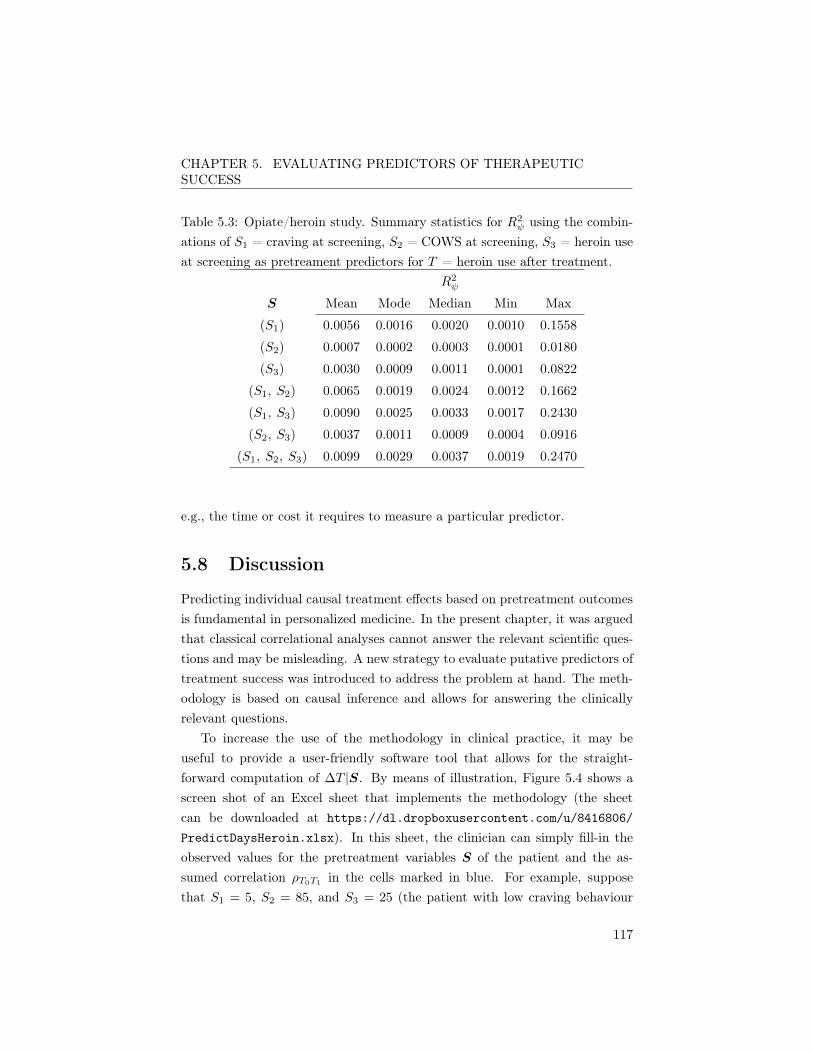
CHAPTER 5. EVALUATING PREDICTORS OF THERAPEUTICSUCCESS
Table 5.3: Opiate/heroin study. Summary statistics for R2 using the combin-
ations of S1 = craving at screening, S2 = COWS at screening, S3 = heroin useat screening as pretreament predictors for T = heroin use after treatment.
R2
S Mean Mode Median Min Max
(S1) 0.0056 0.0016 0.0020 0.0010 0.1558
(S2) 0.0007 0.0002 0.0003 0.0001 0.0180
(S3) 0.0030 0.0009 0.0011 0.0001 0.0822
(S1, S2) 0.0065 0.0019 0.0024 0.0012 0.1662
(S1, S3) 0.0090 0.0025 0.0033 0.0017 0.2430
(S2, S3) 0.0037 0.0011 0.0009 0.0004 0.0916
(S1, S2, S3) 0.0099 0.0029 0.0037 0.0019 0.2470
e.g., the time or cost it requires to measure a particular predictor.
5.8 Discussion
Predicting individual causal treatment effects based on pretreatment outcomesis fundamental in personalized medicine. In the present chapter, it was arguedthat classical correlational analyses cannot answer the relevant scientific ques-tions and may be misleading. A new strategy to evaluate putative predictors oftreatment success was introduced to address the problem at hand. The meth-odology is based on causal inference and allows for answering the clinicallyrelevant questions.
To increase the use of the methodology in clinical practice, it may beuseful to provide a user-friendly software tool that allows for the straight-forward computation of �T |S. By means of illustration, Figure 5.4 shows ascreen shot of an Excel sheet that implements the methodology (the sheetcan be downloaded at https://dl.dropboxusercontent.com/u/8416806/PredictDaysHeroin.xlsx). In this sheet, the clinician can simply fill-in theobserved values for the pretreatment variables S of the patient and the as-sumed correlation ⇢T0T1 in the cells marked in blue. For example, supposethat S1 = 5, S2 = 85, and S3 = 25 (the patient with low craving behaviour
117

CHAPTER 5. EVALUATING PREDICTORS OF THERAPEUTICSUCCESS
Craving at screening
Rψ2
Percentage
0.00 0.05 0.10 0.15 0.20 0.25 0.30
0.0
0.2
0.4
0.6
0.8
COWS at screening
Rψ2
Percentage
0.00 0.05 0.10 0.15 0.20 0.25 0.30
0.0
0.2
0.4
0.6
0.8
Heroin use at screening
Rψ2
Percentage
0.00 0.05 0.10 0.15 0.20 0.25 0.30
0.0
0.2
0.4
0.6
0.8
Craving + COWS at screening
Rψ2
Percentage
0.00 0.05 0.10 0.15 0.20 0.25 0.30
0.0
0.2
0.4
0.6
0.8
Craving + heroin use at screening
Rψ2
Percentage
0.00 0.05 0.10 0.15 0.20 0.25 0.30
0.0
0.2
0.4
0.6
0.8
COWS + heroin use at screening
Rψ2
Percentage
0.00 0.05 0.10 0.15 0.20 0.25 0.30
0.0
0.2
0.4
0.6
0.8
Craving + COWS + heroin use at screening
Rψ2
Percentage
0.00 0.05 0.10 0.15 0.20 0.25 0.30
0.0
0.2
0.4
0.6
0.8
Figure 5.3: Distributions of R2 using the combinations of S1 = craving at
screening, S2 = COWS at screening, S3 = heroin use at screening as pre-treament predictors and T = heroin use after treatment.
118

CHAPTER 5. EVALUATING PREDICTORS OF THERAPEUTICSUCCESS
Figure 5.4: Excel sheet for user-friendly prediction of �Tj | S and its 95%
support interval.
in the example given in Section 5.7) and it is assumed that ⇢T0T1 = 0.125.After filling in these values in the Excel sheet, the output shows the expected�T | S = 0.4567 and 95% support interval [�24.0090; 24.9225]. Further, to-wards the end of the sheet, the conclusion of the analysis is explicitly stated,i.e., the expected �T for this patient is positive and thus the control treatmentis expected to be more beneficial than the experimental treatment though thedifference between the treatments is not significant (the 95% support intervalcontains zero).
The proposed methodology also has some limitations. For example, onlycontinuous and normally distributed pretreatment predictors and true end-points were considered. Other type of variables (e.g., binary) are also oftenencountered in medical applications, and future research should be directed togeneralize the methodology to other outcome types.
Second, MI was used to deal with the missing T0 and T1. This may raisethe question whether the imputed values can also be used to get direct es-timates of ⇢T0T1 . This is however not the case. Indeed, T0 and T1 are neversimultaneously observed and consequently the data at hand do not contain anyinformation about the correlation between the potential outcomes. Therefore,any information about this parameter in the imputed data sets will necessarily
119

CHAPTER 5. EVALUATING PREDICTORS OF THERAPEUTICSUCCESS
come from the imputation model. So basically one would need to impute thedata using several imputation models that assume different values for ⇢T0T1 inorder to avoid bias. Although more laborious, this approach would be equival-ent to the sensitivity analysis that we used and, therefore, multiple imputationdoes not seem to be a better strategy in this scenario.
120

Chapter 6
Evaluating surrogacy in the
meta-analytic framework:
computational issues
6.1 Introduction
The meta-analytic approach to evaluate surrogate endpoints was introducedin Chapters 1 and 3. This framework provides an elegant formalism in whichtwo levels of surrogacy are distinguished: (i) trial-level surrogacy, which essen-tially quantifies the strength of the association between the expected causaltreatment effects on S and the expected causal treatment effects on T , and (ii)individual-level surrogacy, which essentially quantifies the treatment- and trial-corrected strength of association between S and T . These metrics of surrogacycan be obtained by fitting model (1.13) to the data of multiple clinical trials,but unfortunately fitting this model often poses a considerable computationalburden (see also the case study analyses in Chapter 3).
In Section 6.2, it will be examined which factors affect the convergence ofmixed-effects models similar to model (1.13) using simulations. In Section 6.3,it will be examined whether model convergence problems can be amelioratedby using multiple imputation (MI). In Section 6.4, the MI-based approch toreduce model convergence issues is applied in case studies. Finally, in Section
121

CHAPTER 6. EVALUATING SURROGACY IN THE META-ANALYTICFRAMEWORK: COMPUTATIONAL ISSUES
6.5 the results are further discussed.
6.2 Linear mixed-effects models and conver-
gence issues
Fitting a LMM is typically done using Newton-Raphson or quasi-Newton basedprocedures (for details, see Lindstrom and Bates, 1988). Based on some start-ing values for the parameters at hand, these procedures iteratively update theparameter estimates until sufficient convergence is achieved. Unfortunately,non-converging iteration processes often occur when complex LMMs are con-sidered. This means that the iterative process does not converge at all, or thatit converges to values that are close to or outside the boundary of the parameterspace (i.e., variances that are close to zero or negative). The latter issue maylead to a non-positive definite variance-covariance matrix of the random effectsD). Such problems mainly occur in complex hierarchical models (Verbeke andMolenberghs, 2000). In a surrogate evaluation context, the (S, T ) endpoints(level 1) are nested within patients (level 2), and the patients are nested withinclinical trials (or other relevant clustering units; level 3). Given the relativelycomplex hierarchical structure of the data, it is hardly surprising that conver-gence problems are frequently encountered in a surrogate evaluation contextwhen model (1.13) is fitted to the data. For example, convergence problemswere encountered in the analysis of the schizophrenia case study in the meta-analytic framework (see Section 3.4). In fact, to our knowledge there is noreal-life case study available in the surrogate evaluation literature in whichfitting model (1.13) was without problems. To deal with these convergenceissues, Tibaldi et al. (2003) proposed several simplified model fitting strategiesthat can be used when model convergence issue occur. For example, one canreplace the mixed-effects model (1.13) by its fixed-effects counterpart, or the(mixed- or fixed-) bivariate model can be replaced by (mixed- or fixed-) uni-variate models (for details, see Burzykowski, Molenberghs and Buyse, 2005;Alonso et al., 2016; Tibaldi et al., 2003). However, the use of such simplifiedmodel fitting strategies is not always ideal. For example, when the mixed-effects model (1.13) is replaced by its fixed-effects counterpart, patients whohave a missing value in either S or T are removed from the analysis. Therefore,
122

CHAPTER 6. EVALUATING SURROGACY IN THE META-ANALYTICFRAMEWORK: COMPUTATIONAL ISSUES
it would be worthwhile to understand which factors affect the convergence ofthe mixed-effects models similar to model (1.13).
6.2.1 Earlier simulation studies
To gain more insight into the factors that affect convergence of mixed-effectsmodels like (1.13), Buyse et al. (2000) and Renard et al. (2002) conducted anumber of simulation studies. Their conclusion was that model convergencerates were higher (i) when the number of available trials increased, and (ii)when the size of the between-trial variability D increased relative to the re-sidual variability ⌃. Other factors, such as the number of patients per trial,the normality assumption (for S and T ), and the strength of the correlationbetween the random treatment effects had no substantial impact on modelconvergence rates.
6.2.2 Potential relevance of balance in trial size
In the current chapter, the results of the earlier simulation studies (Buyse etal., 2000; Renard et al., 2002) are further extended by evaluating the effect ofan additional factor that may affect model convergence, i.e., imbalance in trialsize. In the earlier simulation studies, balanced datasets were considered, i.e.,all trials had exactly the same number of observations. However, in real-lifedatasets, it is nearly always the case that the trial sizes are unbalanced. Infact, even when a balanced design was initially planned, the actually collecteddata will often be unbalanced due to e.g., missingness.
To understand why balance in trial size may be a relevant factor to consider,recall that the key computational difficulty in fitting mixed-effects models is inthe estimation of the covariance parameters (Verbeke and Molenberghs, 2000).Iterative numerical optimization of the log-likelihood functions using (restric-ted) maximum likelihood estimation is conducted, subject to constraints thatare imposed on the model parameters to ensure positive definiteness of the cov-ariance matrix of the random effects D and of Vi = ZiDZ
0
i+⌃i (where Zi arematrices of known covariates associated with the random effects). Notice thatpositive definiteness of both D and Vi is not needed when one is merely inter-ested in the marginal model. In the latter case, the only requirement for validinference based on the marginal model is that the overall V matrix is positive
123

CHAPTER 6. EVALUATING SURROGACY IN THE META-ANALYTICFRAMEWORK: COMPUTATIONAL ISSUES
definite (see also Section 6.5). To maximize complicated likelihoods or to findgood starting values that can subsequently be used in the Newton-Raphsonalgorithm, the Expectation Maximization (EM) algorithm is often used (De-mpster, Laird and Rubin, 1977). When unbalanced data are considered, theE-step involves, at least conceptually, the creation of a ‘balanced’ dataset (or a‘complete’ dataset in a missing data context; Molenberghs and Kenward, 2007)based on a hypothetical scenario where it is assumed that data were obtainedfrom a balanced design (or from a study in which there are no missing values ina missing data context (Verbeke and Molenberghs, 2000; West, Welch and Ga-lecki, 2015). Based on the ‘balanced’ data, an objective function is constructedand maximized in the M-step, and the parameter estimates are subsequentlyiteratively updated. In essence, the underlying assumption behind the EM al-gorithm is that the optimization of the balanced (complete) data log-likelihoodfunction is easier than the optimization of the unbalanced (observed) datalog-likelihood (West, Welch and Galecki, 2015). In the same spirit, it can beexpected that model convergence issues will occur more frequently when theactually observed data are unbalanced in trial size, compared to the settingwhere the actually observed data are balanced. In the next section, this issuewill be examined using simulations.
6.2.3 Simulations
Three mixed-effects models with an increasing level of complexity were con-sidered: (i) a random-intercept model, (ii) a reduced surrogate evaluationmodel (i.e., a simplification of model (1.13) where the fixed- and random-treatment effects are discarded), and (iii) a surrogate evaluation model (i.e.,model (1.13)). The idea is to gradually build-up the (hierarchical) complex-ity of the model, so that it can be examined at which level of complexity theimpact of an imbalance in trial size on model convergence becomes apparent.
6.2.3.1 Outcomes of interest
The key outcome of interest in the simulations was model convergence. Threemodel convergence categories were distinguished: (i) proper convergence, i.e.,the model converged and the variance-covariance matrix of the random effects(D) and the final Hessian (H), used to compute the standard errors of the
124

CHAPTER 6. EVALUATING SURROGACY IN THE META-ANALYTICFRAMEWORK: COMPUTATIONAL ISSUES
covariance parameters, were positive definite (PD), (ii) the model convergedbut D or H was not PD, and finally, (iii) divergence. In addition, the numberof required iterations to achieve convergence was recorded and analysed.
6.2.3.2 Simulation design
Random-intercept model Consider the following random-intercept model
Sij = µS +mSi + "Sij , (6.1)
where Sij is a (normally distributed) endpoint for patient j in trial i, µS isthe fixed intercept, mSi is the corresponding random intercept, and "Sij is theerror term. It is assumed that mSi ⇠ N(0, d) and "Sij ⇠ N(0, �SS).
In all simulations, µS = 450, �SS = 300, and the mean sample size pertrial M(ni) = 20. Three conditions were varied. First, the number of trialsi = 1, 2, ..., N , with N = {5, 10, 20, 50}. Second, the level of imbalancein trial size (ni). In the balanced scenario, all trial sizes were equal, i.e.,ni = n = 20. In the two unbalanced scenarios, eni was determined based ona draw from a normal distribution and rounded to the nearest integer (i.e.,ni = round ( eni)). In the low imbalance scenario, eni ⇠ N
�20, 2.52
�. In the
high imbalance scenario, eni ⇠ N�20, 52
�. Third, the between-trial variability
(d = �(1, 000)), which is either large (� = 1) or small (� = 0.1) relative tothe residual variability (�SS = 300). There were thus a total of 24 possiblescenarios, for each of which 1, 000 datasets were generated. These dataset weresubsequently analysed by fitting model (6.1) using the mixed procedure in SAS,and model convergence and the required number of iterations were recorded(see Section 6.2.3.1).
Reduced surrogate evaluation model Consider the following LMM(
Sij = µS +mSi + "Sij
Tij = µT +mTi + "Tij
, (6.2)
where Sij and Tij are the (normally distributed) S and T endpoints for patientj in trial i, µS , µT are the fixed intercepts for S and T , mSi, mTi are thecorresponding random intercepts, and "Sij , "Tij are the error terms. It isassumed that (mSi, mTi) ⇠ N (0, D) and ("Sij , "Tij) ⇠ N (0, ⌃), where D
125

CHAPTER 6. EVALUATING SURROGACY IN THE META-ANALYTICFRAMEWORK: COMPUTATIONAL ISSUES
and ⌃ are unstructured 2 by 2 variance-covariance matrices. As can be seen,model (6.2) is a simplification of model (1.13), where the fixed- and random-treatment effects are omitted. Using model (6.2), data were simulated. In allsimulations, µS = 450, µT = 500, and
⌃ =
300 212.132
212.132 300
!,
yielding corr ("Sij , "Tij)2= 0.5. Three conditions were varied in the simu-
lations. First, the number of trials N = {5, 10, 20, 50}. Second, the level ofimbalance in ni (same scenarios as for the random-intercept model). Third, thebetween-trial variability (D), which is either large (� = 1) or small (� = 0.1)relative to the residual variability (⌃)
D = �
1, 000 400
400 1, 000
!.
For each of the 24 settings a total of 1, 000 datasets were generated, and modelconvergence and the required number of iterations were recorded (see Section6.2.3.1).
Surrogate evaluation model Using model (1.13) detailed above, data weresimulated. Notice that Zij was coded as �1 = control treatment and 1 = exper-imental treatment (rather than as 0 = control treatment and 1 = experimentaltreatment), and thus the fixed treatment effects on S and T are 2↵ and 2�,respectively. This was done because a 0/1 coding, for a positive-definite D
matrix, forces the variability in the experimental arm to be greater than orequal to the variability in the control arm. A �1/1 coding on the other handensures that the same components of variability operate in both treatmentarms (Burzykowski, Molenberghs and Buyse, 2005).
In all simulations, µS = 450, µT = 500, ↵ = 300, � = 500, and
⌃ =
300 212.132
212.132 300
!,
yielding R2indiv = corr ("Sij , "Tij)
2= 0.5. Again, three conditions were varied
in the simulations. First, the number of trials N = {5, 10, 20, 50}. Second,
126

CHAPTER 6. EVALUATING SURROGACY IN THE META-ANALYTICFRAMEWORK: COMPUTATIONAL ISSUES
the level of imbalance in ni (same scenarios as for the random-intercept model).Third, the between-trial variability (D), which is either large (� = 1) or small(� = 0.1) relative to the residual variability (⌃)
D = �
0
BBBBB@
1, 000 400 0 0
400 1, 000 0 0
0 0 1, 000 707.107
0 0 707.107 1, 000
1
CCCCCA,
yielding R2trial = corr (ai, bi)2 = 0.5. Further, in the balanced scenario, treat-
ment (Z) is also balanced within a trial. In the unbalanced scenarios, treatmentallocation is determined based on a binomial distribution with success probab-ility 0.50. A total of 1, 000 datasets were generated for each of the 24 settings.The generated data were subsequently analysed by fitting Model (1.13) in SAS.
Two different parametrizations for the D matrix were considered. First, acompletely general (unstructured; UN) D matrix that is parametrized directlyin terms of variances and covariances. Second, a non-diagonal factor-analyticstructure with 4 factors (FA0(4)). The latter structure specifies a Choleskyroot parametrization for the 4 ⇥ 4 unstructured D matrix. This leads to asubstantial simplification of the optimization problem, i.e., the problem nowchanges from a constrained one to an unconstrained one. The FA0(4) struc-ture has q
2 (2t� q + 1) covariance parameters, where q refers to the numberof factors and t is the dimension of the matrix. In the present setting, theFA0(4) structure thus has a total of 10 parameters. These parameters are usedto compute the components in D, i.e., the (i, j)th element of D is computedas ⌃
min(i,j,k)k=1 �ik�jk. The Cholesky root parametrization ensures that D (and
Vi) is positive definite during the entire estimation process (West, Welch andGalecki, 2015). Model convergence and the required number of iterations wererecorded (see Section 6.2.3.1).
6.2.3.3 Results
As shown in Table 6.1, the rates of proper convergence exceeded 0.960 and0.841 in the various scenarios for the random-intercept and reduced surrogatemodels, respectively. Overall convergence (i.e., proper convergence or conver-gence but non-PD D or H matrix) was 100% for the random-intercept model
127

CHAPTER 6. EVALUATING SURROGACY IN THE META-ANALYTICFRAMEWORK: COMPUTATIONAL ISSUES
and � 97.8% for the reduced surrogate model. The rates of proper and overallconvergence were similar in all scenarios, irrespective of the level of imbalancein trial size (ni). However, a larger level of imbalance in trial size was associatedwith a higher mean number of iterations that were required to achieve properconvergence for both the random-intercept and the reduced surrogate models(see Table 6.2). This suggests that the optimization of the log-likelihood func-tion is more difficult in the unbalanced scenarios, even when relatively simplemixed-effects models (in terms of their hierarchical structure) are considered.
When an unstructured (UN) D matrix was used in the surrogate evaluationmodels, overall convergence exceeded 99.7% when trial sizes were balanced (seeTable 6.1). The overall convergence rates were, however, substantially lower inthe unbalanced scenarios, in particular when N and � were small. For example,when N = 5 and � = 0.1, the model divergence rates were as high as 65.5%
and 77.3% in the small and large imbalance scenarios, respectively (comparedto only 0.3% in the balanced scenario). At the same time, the impact of levelof imbalance on proper convergence was small, i.e., proper convergence rateswere quite similar in all scenarios irrespective of the level of imbalance in thedata.
When a non-diagonal factor analytic structure with 4 factors (FA0(4)) wasused for the D matrix in the surrogate evaluation models, the rates of properconvergence exceeded 71.0% in all scenarios (see Table 6.1) and were thus sub-stantially higher compared to those that were observed in the UN scenario.Further, divergence rates were substantially lower in the unbalanced FA0(4)scenarios compared to those in the unbalanced UN scenarios. As was also ob-served for the random-intercept and the reduced surrogate models, a higherlevel of imbalance in trial size was associated with a larger mean number ofrequired iterations to achieve proper convergence for both the UN and FA0(4)surrogate evaluation models (see Table 6.2). A noteworthy observation is thatproper convergence was always achieved after 1 iteration when the trial sizewas balanced for the random-intercept, reduced surrogate, and UN surrogateevaluation models (Table 6.2). The reverse also holds approximately, i.e., whena model converged after 1 iteration, in more than 99.9% of the cases there wasproper convergence. In contrast to what was the case for the UN surrogateevaluation models, proper convergence was not always achieved after 1 itera-tion for the FA0(4) surrogate evaluation models. Nonetheless, the number of
128

CHAPTER 6. EVALUATING SURROGACY IN THE META-ANALYTICFRAMEWORK: COMPUTATIONAL ISSUES
required iterations to achieve proper convergence was also substantially lowerin the balanced FA0(4) surrogate evaluation models compared to what was thecase in the unbalanced FA0(4) surrogate evaluation models.
6.3 Balanced cluster sizes and multiple imputa-
tion
Based on the reasoning in Section 6.2.2, it can be hypothesized that the useof MI to make unbalanced datasets ‘balanced’ prior to fitting the mixed-effectsmodel would ameliorate convergence problems. This issue is examined in thepresent section based on simulations.
6.3.1 Simulations
6.3.1.1 Simulation design
The same unbalanced datasets that were generated in the surrogate evaluationmodel scenario described above (see Section 6.2.3.2) were considered here. Inthese unbalanced datasets, MI was used to introduce balance in terms of trialsize and treatment allocation (Z). As an example of what is meant by this,consider the hypothetical dataset with 5 trials shown in Table 6.3. As canbe seen, the maximum number of patients for each of the trial by treatment(Z) groups is 18. Thus for all trial ⇥ treatment groups having less than 18
observations, MI is used to restore balance. For example, in trial 1 there were5 observations for S and T in treatment group Z = �1 and 11 observations intreatment group Z = 1. Thus, the data of 13 and 7 patients are imputed intrial 1 for Z = �1 and Z = 1, respectively.
Multivariate imputations were conducted using the default Markov chainMonte Carlo method (Schafer, 1997) in SAS with a non-informative prior (Jef-freys). The imputation model included S, T , and Z. The imputation modelwas run ‘by trial’. A total of 200 burn-in iterations were used (i.e., the num-ber of initial iterations before the first iteration for a chain), and the numberof iterations between the imputations in a chain equalled 100. A total of 3
imputations were conducted for each dataset. Thus in total, 24, 000 datasetswere considered in the analyses (i.e., 4 (number of N) · 2 (number of �) · 1, 000
129

CHAPTER 6. EVALUATING SURROGACY IN THE META-ANALYTICFRAMEWORK: COMPUTATIONAL ISSUES
Table6.1:
Convergence
ratesfor
therandom
-interceptm
odels,reduced
surrogatem
odels,and
surrogatem
odelsas
afunction
ofbalancednessof
ni ,the
number
oftrials(5,10,20,
50)
andthe
between-trialvariability.
Model
Balanced
(equalni )
Smallim
balanceLarge
imbalance
eni⇠
N�20,2.5
2 �eni⇠
N�20,
5
2 �
Convergence
Betw
een-trialN
umber
oftrialsN
umber
oftrialsN
umber
oftrialscategory
variability�
510
20
50
510
20
50
510
20
50
Random
Proper
convergenceSm
all(0.1)
0.974
0.999
11
0.969
0.999
11
0.960
0.998
11
interceptLarge
(1)
0.999
11
10.997
11
10.989
11
1
Convergence
butSm
all(0.1)
0.026
0.001
00
0.031
0.001
00
0.040
0.002
00
non-PD
D/H
matrix
Large(1)
0.001
00
00.003
00
00.011
00
0
Divergence
Small(
0.1)
00
00
00
00
00
00
Large(1)
00
00
00
00
00
00
Convergence
Betw
een-trialN
umber
oftrialsN
umber
oftrialsN
umber
oftrials
categoryvariability
�5
10
20
50
510
20
50
510
20
50
Reduced
surrogateP
roperconvergence
Small(
0.1)
0.853
0.991
11
0.853
0.990
11
0.841
0.987
11
model
Large(1)
0.990
11
10.992
11
10.995
11
1
Convergence
butSm
all(0.1)
0.147
0.009
00
0.141
0.010
00
0.137
0.013
00
non-PD
D/H
matrix
Large(1)
0.010
00
00.007
00
00.004
00
0
Divergence
Small(
0.1)
00
00
0.006
00
00.022
00
0
Large(1)
00
00
0.001
00
00.001
00
0
Convergence
Betw
een-trialN
umber
oftrialsN
umber
oftrialsN
umber
oftrialscategory
variability�
510
20
50
510
20
50
510
20
50
Surrogatem
odel,P
roperconvergence
Small(
0.1)
0.112
0.826
0.999
10.090
0.816
11
0.091
0.800
0.999
1
UN
Large(1)
0.555
0.998
11
0.566
0.999
11
0.540
0.996
11
Convergence
butSm
all(0.1)
0.885
0.174
0.001
00.255
0.171
00
0.136
0.155
0.001
0
non-PD
D/H
matrix
Large(1)
0.444
0.002
00
0.163
0.001
00
0.119
0.001
00
Divergence
Small(
0.1)
0.003
00
00.655
0.013
00
0.773
0.045
00
Large(1)
0.001
00
00.271
00
00.341
0.003
00
Surrogatem
odel,P
roperconvergence
Small(
0.1)
0.745
0.984
11
0.717
0.976
11
0.710
0.976
0.999
1
FA0(4)
Large(1)
0.931
11
10.931
0.994
0.997
0.998
0.935
0.992
0.998
0.999
Convergence
butSm
all(0.1)
0.068
0.007
00
0.054
0.016
00
0.044
0.015
00
non-PD
D/H
matrix
Large(1)
0.030
00
00.027
0.001
0.002
00.018
0.004
0.001
0.001
Divergence
Small(
0.1)
0.187
0.009
00
0.229
0.008
00
0.246
0.009
0.001
0
Large(1)
0.039
00
00.042
0.005
0.001
0.002
0.047
0.004
0.001
0
Note.
UN
=unstructured;FA
0(4)=
factoranalytic
130

CHAPTER 6. EVALUATING SURROGACY IN THE META-ANALYTICFRAMEWORK: COMPUTATIONAL ISSUES
Tabl
e6.
2:M
ean
(SD
)num
bero
fite
rati
onsp
erco
nver
genc
eca
tego
ryfo
rthe
rand
om-in
terc
eptm
odel
s,th
ere
duce
dsu
rrog
ate
mod
els,
and
the
surr
ogat
em
odel
sas
afu
ncti
onof
bala
nced
ness
ofni,
the
num
ber
oftr
ials
(5,10,20,50)
and
the
betw
een-
tria
lvar
iabi
lity.
Mod
elB
alan
ced
(equ
alni)
Smal
lim
bala
nce
Larg
eim
bala
nce
en i⇠
N� 20,2.5
2�
en i⇠
N� 20,5
2�
Con
verg
ence
Bet
wee
n-tr
ial
Num
ber
oftr
ials
Num
ber
oftr
ials
Num
ber
oftr
ials
cate
gory
vari
abili
ty�
510
20
50
510
20
50
510
20
50
Ran
dom
Pro
per
conv
erge
nce
Smal
l(0.1
)1(0)
1(0)
1(0)
1(0)
2.18(0.85)
2.22(0.80)
2.09(0.73)
1.88(0.63)
2.70(1.06)
2.71(0.95)
2.52(0.87)
2.32(0.78)
inte
rcep
tLa
rge
(1)
1(0)
1(0)
1(0)
1(0)
2.91(1.31)
2.95(1.14)
2.82(1.02)
2.56(0.84)
3.70(1.89)
3.85(1.85)
3.64(1.68)
3.13(1.04)
Con
verg
ence
but
Smal
l(0.1
)1(0)
1(�)
��
1(0)
1(�)
��
1(0)
1(0)
��
non-
PD
D/H
mat
rix
Larg
e(1
)1(�)
��
�1(0)
��
�1(0)
��
�
Div
erge
nce
Smal
l(0.1
)�
��
��
��
��
��
�
Larg
e(1
)�
��
��
��
��
��
�
Con
verg
ence
Bet
wee
n-tr
ial
Num
ber
oftr
ials
Num
ber
oftr
ials
Num
ber
oftr
ials
cate
gory
vari
abili
ty�
510
20
50
510
20
50
510
20
50
Red
uced
surr
ogat
eP
rope
rco
nver
genc
eSm
all(
0.1
)1(0)
1(0)
1(0)
1(0)
2.67(0.78)
2.59(0.70)
2.35(0.58)
2.08(0.44)
3.51(1.02)
3.37(0.89)
3.06(0.77)
2.66(0.65)
mod
elLa
rge
(1)
1(0)
1(0)
1(0)
1(0)
4.06(1.78)
4.12(1.72)
3.84(1.35)
3.32(0.79)
5.36(2.30)
5.42(2.32)
5.11(2.36)
4.28(1.51)
Con
verg
ence
but
Smal
l(0.1
)4.28(1.61)
3.22(0.67)
��
4.38(1.47)
4.10(0.88)
��
4.46(1.44)
4.15(1.46)
��
non-
PD
D/H
mat
rix
Larg
e(1
)4.20(1.40)
��
�4.14(1.35)
��
�5.50(2.53)
��
�
Div
erge
nce
Smal
l(0.1
)�
��
�36.17(6.31)
��
�50.46(58.29)
��
�
Larg
e(1
)�
��
�44.00(�)
��
�36.00(�)
��
�
Con
verg
ence
Bet
wee
n-tr
ial
Num
ber
oftr
ials
Num
ber
oftr
ials
Num
ber
oftr
ials
cate
gory
vari
abili
ty�
510
20
50
510
20
50
510
20
50
Surr
ogat
em
odel
,P
rope
rco
nver
genc
eSm
all(
0.1
)1(0)
1(0)
1(0)
1(0)
4.99(1.14)
4.30(0.85)
3.70(0.73)
3.11(0.58)
5.34(1.12)
4.72(0.86)
4.15(0.70)
3.52(0.67)
UN
Larg
e(1
)1(0)
1(0)
1(0)
1(0)
7.68(2.60)
6.73(2.49)
5.84(2.43)
4.69(1.75)
8.21(2.40)
7.35(2.67)
6.67(2.63)
5.54(2.32)
Con
verg
ence
but
Smal
l(0.1
)9.16(9.06)
3.97(1.37)
4(�)
�6.85(2.13)
5.34(1.34)
��
6.73(1.83)
5.56(1.32)
5(�)
�
non-
PD
D/H
mat
rix
Larg
e(1
)6.35(3.50)
3.50(2.12)
��
9.90(2.71)
8.00(�)
��
9.57(2.61)
8.00(�)
��
Div
erge
nce
Smal
l(0.1
)309.33(306.91)
��
�50.10(16.51)
49.00(12.17)
��
47.66(15.01)
48.81(16.05)
��
Larg
e(1
)205.00(�)
��
�50.79(19.71)
��
�49.40(15.39)
44.00(2.00)
��
Surr
ogat
em
odel
,P
rope
rco
nver
genc
eSm
all(
0.1
)4.90(3.90)
1.66(1.87)
1(0.09)
1(0)
6.00(2.99)
4.37(3.16)
2.87(0.62)
2.36(0.49)
6.45(3.31)
4.94(3.38)
3.29(1.20)
2.77(0.52)
FA0(
4)La
rge
(1)
2.24(1.19)
1.01(0.16)
1(0)
1(0)
9.54(7.69)
6.36(3.42)
5.67(3.33)
4.65(2.27)
10.87(8.57)
6.98(4.54)
6.27(3.08)
5.40(2.61)
Con
verg
ence
but
Smal
l(0.1
)6.12(1.94)
5.71(2.21)
��
6.91(2.05)
5.69(1.45)
��
6.55(1.30)
5.80(1.93)
��
non-
PD
D/H
mat
rix
Larg
e(1
)5.13(1.68)
��
�11.85(7.48)
20(�)
23.50(0.71)
�13.39(14.14)
24(16.67)
23(�)
38(�)
Div
erge
nce
Smal
l(0.1
)21.96(13.84)
30.78(12.13)
��
19.41(11.75)
18.25(9.77)
��
20.10(12.88)
32.33(18.32)
49(0)
�
Larg
e(1
)31.67(11.43)
��
�29.57(13.46)
27(11.98)
11(�)
17(5.66)
27.87(11.82)
29.50(21.61)
9(�)
�
Not
e.U
N=
unst
ruct
ured
;FA
0(4)
=fa
ctor
anal
ytic
.
131

CHAPTER 6. EVALUATING SURROGACY IN THE META-ANALYTICFRAMEWORK: COMPUTATIONAL ISSUES
Table 6.3: Hypothetical dataset. Number of observations per trial as a functionof treatment (Z), before and after imputation.
Before imputation After imputation
trial Z = �1 Z = 1 Z = �1 Z = 1
1 5 11 18 18
2 13 8 18 18
3 10 18 18 18
4 9 5 18 18
5 9 11 18 18
(number of runs) · 3 (number of imputations)) for both the small imbalanceand the large imbalance scenarios. The ‘balanced’ data were subsequently ana-lysed by fitting model (1.13) using the UN and FA0(4) parametrizations forthe D matrix (see Section 6.2.3.2).
6.3.1.2 Outcomes of interest
The outcomes of interest were model convergence and the number of requirediterations to achieve convergence (see Section 6.2.3.1). In addition, the bias,efficiency (standard deviation of the estimate) and Mean Squared Errors ofthe estimates of the R2
trial and R2indiv metrics were evaluated. The focus was
on R2trial and R2
indiv rather than on the fixed-effects and separate variancecomponents because these coefficients of determination are the main quantitiesof interest in a meta-analytic surrogate evaluation context. Notice that thecomputation of R2
trial simplifies here to R2trial = Rbi|ai
=
d2ab
daadbb, because it is
assumed that there is no heterogeneity in the random intercepts for S and T .
6.3.1.3 Results
Table 6.4 shows the convergence rates for the MI UN and MI FA0(4) models.Compared to what was the case for the surrogate evaluation models in theunbalanced non-MI scenarios, the rates of proper and overall convergence weresubstantially higher in both the MI UN and MI FA0(4) scenarios – and this
132

CHAPTER 6. EVALUATING SURROGACY IN THE META-ANALYTICFRAMEWORK: COMPUTATIONAL ISSUES
was particularly so when N was small. The use of MI to make the unbalanceddata balanced was thus a successful strategy to improve convergence rates andreduce divergence.
In line with the results discussed in Section 6.2.3.3, proper convergencewas always achieved after 1 iteration in the MI UN scenario but not in the MIFA0(4) scenario (see Table 6.5). Nonetheless, the number of required iterationsto achieve convergence was substantially reduced in the unbalanced MI FA0(4)scenarios compared to what was the case in the non-MI unbalanced scenarios(compare Tables 6.2 and 6.5).
Tables 6.6 and 6.7 show the bias, efficiency, and MSE of the estimates ofR2
indiv and R2trial, respectively, in the non-MI and MI settings that properly
converged. As expected, the bias, efficiency and MSE in the estimation ofboth R2
indiv and R2trial improved when the number of trials increased. With
respect to the estimation of R2indiv, the bias was low in all scenarios but the
efficiency and MSE were poorer in the MI scenarios compared to the non-MI scenarios. In contrast to R2
indiv, the bias, efficiency and MSE were ofsimilar magnitude in the MI and non-MI scenarios for R2
trial. Only when N =
5 did the bias in the estimation of R2trial tend to be substantially higher in
the MI scenario compared to the non-MI scenario. Note that the bias wasnegative in all scenarios, indicating that the true R2
trial tends to be somewhatunderestimated.
Further, the bias and MSE in the estimation of R2indiv was smaller compared
to what was observed for R2trial, and the efficiency somewhat lower. This result
was expected, as there is less replication at the trial level than at the individuallevel of analysis.
6.4 Case studies
The results that were detailed in Section 6.3 indicated that the use of MI to‘balance’ an unbalanced dataset prior to fitting the mixed-effects model (1.13)reduces model convergence issues. Here, this method is applied in the analysisof two real-life case studies, i.e., the ARMD and schizophrenia trials.
133

CHAPTER 6. EVALUATING SURROGACY IN THE META-ANALYTICFRAMEWORK: COMPUTATIONAL ISSUES
Table6.4:
Convergence
ratesfor
thesurrogate
MIU
N(unstructured)
andM
IFA0(4)
(factoranalytic)
models
asa
functionofbalancedness
ofni ,the
number
oftrials(5,
10,
20,50)
andthe
between-trialvariability.
Model
Smallim
balanceLarge
imbalance
eni⇠
N�20,2.5
2 �eni⇠
N�20,
5
2 �
Convergence
Betw
een-trialN
umber
oftrialsN
umber
oftrialscategory
variability�
510
20
50
510
20
50
Surrogatem
odel,P
roperconvergence
Small(
0.1)
0.164
0.941
11
0.189
0.946
0.999
0.999
MI
UN
Large(1)
0.617
0.999
11
0.616
0.999
0.999
1
Convergence
butSm
all(0.1)
0.811
0.059
00
0.770
0.054
0.001
0.001
non-PD
D/H
matrix
Large(1)
0.365
0.001
00
0.343
0.001
0.001
0
Divergence
Small(
0.1)
0.025
00
00.042
00
0
Large(1)
0.018
00
00.041
00
0
Convergence
Betw
een-trialN
umber
oftrialsN
umber
oftrialscategory
variability�
510
20
50
510
20
50
Surrogatem
odel,P
roperconvergence
Small(
0.1)
0.813
0.998
11
0.817
0.996
0.999
0.999
MI
FA0(4)
Large(1)
0.954
0.999
11
0.950
10.999
1
Convergence
butSm
all(0.1)
0.077
0.002
00
0.072
0.003
00
non-PD
D/H
matrix
Large(1)
0.012
0.001
00
0.022
00.001
0
Divergence
Small(
0.1)
0.109
0.002
00
0.111
0.001
0.001
0
Large(1)
0.029
0.001
00
0.028
00
0
134

CHAPTER 6. EVALUATING SURROGACY IN THE META-ANALYTICFRAMEWORK: COMPUTATIONAL ISSUES
Tabl
e6.
5:M
ean
(SD
)nu
mbe
rof
iter
atio
nspe
rco
nver
genc
eca
tego
ryfo
rth
esu
rrog
ate
MI
UN
(uns
truc
ture
d)an
dM
IFA
0(4)
(fac
tor
anal
ytic
)m
odel
sas
afu
ncti
onof
bala
nced
ness
ofni,
the
num
ber
oftr
ials
(5,10,20,50)
and
the
betw
een-
tria
lvar
iabi
lity.
Not
e.�
:qu
anti
tyca
nnot
beco
mpu
ted.
Mod
elSm
alli
mba
lanc
eLa
rge
imba
lanc
een i
⇠N
(M
=20,SD
=2.5)
en i⇠
N(M
=20,SD
=5)
Con
verg
ence
Bet
wee
n-tr
ial
Num
ber
oftr
ials
Num
ber
oftr
ials
cate
gory
vari
abili
ty�
510
20
50
510
20
50
Surr
ogat
em
odel
,P
rope
rco
nver
genc
eSm
all(
0.1
)1(0)
1(0)
1(0)
1(0)
1(0)
1(0)
1(0)
1(0)
MI
UN
Larg
e(1
)1(0)
1(0)
1(0)
1(0)
1(0)
1(0)
1(0)
1(0)
Con
verg
ence
but
Smal
l(0.1
)8.19(4.61)
3.68(1.35)
��
8.41(17.51)
3.87(1.51)
9.00(�)
8.00(�)
non-
PD
D/H
mat
rix
Larg
e(1
)6.20(3.79)
5.00(0)
��
6.15(4.48)
5.00(�)
2.50(2.12)
�
Div
erge
nce
Smal
l(0.1
)66.93(82.89)
��
�56.49(12.16)
��
�
Larg
e(1
)55.26(8.29)
��
�54.96(17.06)
��
�
Con
verg
ence
Bet
wee
n-tr
ial
Num
ber
oftr
ials
Num
ber
oftr
ials
cate
gory
vari
abili
ty�
510
20
50
510
20
50
Surr
ogat
em
odel
,P
rope
rco
nver
genc
eSm
all(
0.1
)4.24(2.91)
1.22(1.08)
1(0)
1(0)
4.04(2.66)
1.19(0.99)
1(0)
1(0)
MI
FA0(
4)La
rge
(1)
2.06(1.91)
1.00(0.07)
1(0)
1(0)
2.04(1.90)
1.00(0.06)
1(0)
1(0)
Con
verg
ence
but
Smal
l(0.1
)5.92(1.94)
4.50(1.38)
��
5.87(1.99)
4.89(1.17)
��
non-
PD
D/H
mat
rix
Larg
e(1
)4.92(1.19)
4.00(�)
��
4.55(1.30)
�13.50(10.61)
�
Div
erge
nce
Smal
l(0.1
)21.25(12.83)
33.60(7.27)
��
22.18(13.28)
38.75(10.05)
19.00(�)
56.00(�)
Larg
e(1
)35.01(12.00)
37.00(0)
��
32.43(12.87)
��
�
135

CHAPTER 6. EVALUATING SURROGACY IN THE META-ANALYTICFRAMEWORK: COMPUTATIONAL ISSUES
Table6.6:
Bias,
efficiency
andM
SEof
theestim
atesof
R2in
div
inthe
non-MI
andM
Isurrogate
evaluationm
odelsthat
properlyconverged
asa
functionofbalancedness
ofni ,the
number
oftrials(5,10,20,
50)
andthe
between-trialvariability.
Model
Balanced
(equalni )
Smallim
balanceLarge
imbalance
eni⇠
N�20,
2.5
2 �eni⇠
N�20,
5
2 �
Measure
Betw
een-trialN
umber
oftrialsN
umber
oftrialsN
umber
oftrials
variability(�)
510
20
50
510
20
50
510
20
50
Surrogatem
odel,B
iasSm
all(0.1)
�0.001
�0.001
�0.002
0.001
�0.014
0.001
�0.001
0.001
0.009
0.001
�0.002
0.001
non-MI,U
NLarge
(1)
�0.005
�0.001
�0.001
�0.001
�0.009
�0.001
0.001
�0.001
�0.009
�0.001
0.001
�0.001
Effi
ciencySm
all(0.1)
0.080
0.052
0.037
0.023
0.072
0.053
0.037
0.023
0.067
0.052
0.038
0.023
Large(1)
0.072
0.053
0.037
0.024
0.071
0.052
0.037
0.024
0.073
0.052
0.037
0.024
MSE
Small(
0.1)
0.006
0.003
0.001
0.001
0.005
0.003
0.001
0.001
0.004
0.003
0.001
0.001
Large(1)
0.005
0.003
0.001
0.001
0.005
0.003
0.001
0.001
0.005
0.003
0.001
0.001
Measure
Betw
een-trialN
umber
oftrialsN
umber
oftrialsN
umber
oftrials
variability(�)
510
20
50
510
20
50
510
20
50
Surrogatem
odel,B
iasSm
all(0.1)
�0.001
�0.009
�0.002
0.001
�0.001
0.001
�0.001
0.001
�0.001
0.001
�0.002
0.001
non-MI,FA
0(4)Large
(1)
�0.006
�0.001
�0.001
�0.001
�0.007
�0.001
0.001
�0.001
�0.007
�0.001
0.001
�0.001
Effi
ciencySm
all(0.1)
0.074
0.052
0.037
0.023
0.076
0.053
0.037
0.023
0.072
0.051
0.038
0.023
Large(1)
0.073
0.053
0.037
0.024
0.072
0.053
0.037
0.026
0.074
0.052
0.038
0.027
MSE
Small(
0.1)
0.006
0.003
0.001
0.001
0.006
0.003
0.001
0.001
0.005
0.003
0.001
0.001
Large(1)
0.005
0.003
0.001
0.001
0.005
0.003
0.001
0.001
0.006
0.003
0.001
0.001
Measure
Betw
een-trialN
umber
oftrialsN
umber
oftrialsN
umber
oftrials
variability(�)
510
20
50
510
20
50
510
20
50
Surrogatem
odel,B
iasSm
all(0.1)
��
��
�0.005
0.001
�0.001
0.003
0.008
0.004
�0.001
0.004
MI
UN
Large(1)
��
��
�0.005
0.002
0.002
0.001
�0.005
0.001
0.004
0.001
Effi
ciencySm
all(0.1)
��
��
0.089
0.066
0.047
0.030
0.095
0.074
0.057
0.040
Large(1)
��
��
0.087
0.065
0.047
0.031
0.098
0.076
0.057
0.043
MSE
Small(
0.1)
��
��
0.008
0.004
0.002
0.001
0.009
0.005
0.003
0.002
Large(1)
��
��
0.008
0.004
0.002
0.001
0.010
0.006
0.003
0.002
Measure
Betw
een-trialN
umber
oftrialsN
umber
oftrialsN
umber
oftrials
variability(�)
510
20
50
510
20
50
510
20
50
Surrogatem
odel,B
iasSm
all(0.1)
��
��
�0.001
0.001
�0.001
0.003
0.003
0.003
�0.001
0.004
MI
FA0(4)
Large(1)
��
��
�0.005
0.002
0.002
0.001
�0.005
0.001
0.004
0.001
Effi
ciencySm
all(0.1)
��
��
0.090
0.066
0.047
0.030
0.097
0.074
0.057
0.040
Large(1)
��
��
0.097
0.065
0.047
0.031
0.099
0.076
0.057
0.043
MSE
Small(
0.1)
��
��
0.008
0.004
0.002
0.001
0.009
0.006
0.003
0.002
Large(1)
��
��
0.008
0.004
0.002
0.001
0.010
0.006
0.003
0.002
Note.
UN
=unstructured;FA
0(4)=
factoranalytic.
136

CHAPTER 6. EVALUATING SURROGACY IN THE META-ANALYTICFRAMEWORK: COMPUTATIONAL ISSUES
Tabl
e6.
7:B
ias,
effici
ency
and
MSE
ofth
ees
tim
ates
ofR
2 tria
lin
the
non-
MI
and
MI
surr
ogat
eev
alua
tion
mod
els
that
prop
erly
conv
erge
das
afu
nction
ofba
lanc
edne
ssof
ni,
the
num
ber
oftr
ials
(5,10,20,50)
and
the
betw
een-
tria
lvar
iabi
lity.
Mod
elB
alan
ced
(equ
alni)
Smal
lim
bala
nce
Larg
eim
bala
nce
en i⇠
N� 20,2.5
2�
en i⇠
N� 20,5
2�
Mea
sure
Bet
wee
n-tr
ial
Num
ber
oftr
ials
Num
ber
oftr
ials
Num
ber
oftr
ials
vari
abili
ty(�
)5
10
20
50
510
20
50
510
20
50
Surr
ogat
em
odel
,B
ias
Smal
l(0.1
)�0.152
�0.097
�0.041
�0.019
�0.168
�0.093
�0.036
�0.016
�0.174
�0.094
�0.034
�0.002
non-
MI,
UN
Larg
e(1
)�0.168
�0.075
�0.031
�0.013
�0.170
�0.074
�0.031
�0.012
�0.152
�0.074
�0.029
�0.009
Effi
cien
cySm
all(
0.1
)0.254
0.224
0.182
0.111
0.246
0.229
0.184
0.112
0.280
0.232
0.187
0.114
Larg
e(1
)0.248
0.219
0.158
0.095
0.239
0.222
0.157
0.096
0.248
0.221
0.157
0.095
MSE
Smal
l(0.1
)0.087
0.059
0.035
0.013
0.088
0.061
0.035
0.013
0.108
0.063
0.036
0.013
Larg
e(1
)0.089
0.053
0.026
0.009
0.086
0.055
0.026
0.009
0.084
0.054
0.025
0.009
Mea
sure
Bet
wee
n-tr
ial
Num
ber
oftr
ials
Num
ber
oftr
ials
Num
ber
oftr
ials
vari
abili
ty(�
)5
10
20
50
510
20
50
510
20
50
Surr
ogat
em
odel
,B
ias
Smal
l(0.1
)�0.139
�0.090
�0.071
�0.035
�0.157
�0.088
�0.061
�0.032
�0.151
�0.082
�0.057
�0.018
non-
MI,
FA0(
4)La
rge
(1)
�0.099
�0.077
�0.060
�0.024
�0.109
�0.073
�0.063
�0.024
�0.076
�0.071
�0.058
�0.020
Effi
cien
cySm
all(
0.1
)0.267
0.233
0.203
0.121
0.269
0.238
0.197
0.122
0.273
0.237
0.201
0.125
Larg
e(1
)0.272
0.232
0.178
0.101
0.269
0.236
0.179
0.100
0.266
0.234
0.177
0.101
MSE
Smal
l(0.1
)0.090
0.062
0.046
0.016
0.096
0.064
0.043
0.016
0.097
0.063
0.044
0.016
Larg
e(1
)0.084
0.060
0.035
0.011
0.084
0.061
0.036
0.011
0.076
0.060
0.035
0.011
Mea
sure
Bet
wee
n-tr
ial
Num
ber
oftr
ials
Num
ber
oftr
ials
Num
ber
oftr
ials
vari
abili
ty(�
)5
10
20
50
510
20
50
510
20
50
Surr
ogat
em
odel
,B
ias
Smal
l(0.1
)�
��
��0.186
�0.080
�0.034
�0.016
�0.193
�0.087
�0.036
�0.022
MI
UN
Larg
e(1
)�
��
��0.165
�0.071
�0.031
�0.012
�0.163
�0.072
�0.032
�0.018
Effi
cien
cySm
all(
0.1
)�
��
�0.255
0.226
0.172
0.105
0.257
0.229
0.174
0.128
Larg
e(1
)�
��
�0.244
0.221
0.155
0.095
0.254
0.222
0.160
0.108
MSE
Smal
l(0.1
)�
��
�0.099
0.057
0.031
0.011
0.103
0.060
0.031
0.017
Larg
e(1
)�
��
�0.087
0.054
0.025
0.009
0.091
0.054
0.027
0.012
Mea
sure
Bet
wee
n-tr
ial
Num
ber
oftr
ials
Num
ber
oftr
ials
Num
ber
oftr
ials
vari
abili
ty(�
)5
10
20
50
510
20
50
510
20
50
Surr
ogat
em
odel
,B
ias
Smal
l(0.1
)�
��
��0.258
�0.088
�0.034
�0.016
�0.266
�0.094
�0.036
�0.022
MI
FA0(
4)La
rge
(1)
��
��
�0.193
�0.071
�0.031
�0.012
�0.193
�0.072
�0.032
�0.018
Effi
cien
cySm
all(
0.1
)�
��
�0.251
0.228
0.172
0.105
0.251
0.233
0.174
0.128
Larg
e(1
)�
��
�0.253
0.221
0.155
0.095
0.261
0.222
0.160
0.108
MSE
Smal
l(0.1
)�
��
�0.130
0.060
0.031
0.011
0.134
0.063
0.031
0.017
Larg
e(1
)�
��
�0.101
0.054
0.025
0.009
0.106
0.054
0.027
0.011
Not
e.U
N=
unst
ruct
ured
;FA
0(4)
=fa
ctor
anal
ytic
.
137

CHAPTER 6. EVALUATING SURROGACY IN THE META-ANALYTICFRAMEWORK: COMPUTATIONAL ISSUES
6.4.1 The ARMD trial
6.4.1.1 Analysis
The ARMD trial is a multicenter study that enrolled a total of 181 patientsfrom 36 centers (for details, see Section 2.1.3). The meta-analytic approach willbe used to evaluate whether the change in visual acuity after 24 weeks is anappropriate surrogate for the change in visual acuity after 52 weeks. Center wasused as the clustering variable in the analyses. Centers that enrolled less than5 patients were discarded from the analyses. This was done to avoid problemsduring the MI phase, i.e., in line with the procedure described in Section 6.3,the MI was conducted for each center separately and thus a sufficient numberof observations should be available per center. The dataset that was analysedcontained 119 patients from 17 centers. The center that had the largest samplesize included 18 patients, of whom 9 patients received placebo and 9 patientsreceived the experimental treatment. Thus, in all center by treatment groupsthat had less than 9 patients, data were imputed to achieve balance. Theimputations were conducted for each of the centers separately using S, T , andZ in the imputation model. A total of 1, 000 imputations were conducted. Foreach of the imputed datasets, model (1.13) was fitted. Both the FA0(4) andUN covariance parametrizations for D were used.
6.4.1.2 Results
Convergence rates When model (1.13) was fitted to the non-imputed dataof the case study, convergence issues occurred. In particular, the models thatused the UN parametrization for the D matrix did not converge and the modelsthat used the FA0(4) parametrization converged to a non-PD D/H matrix.
Table 6.8 shows the convergence rates that were obtained when the MI-based approaches were used. Overall convergence was high and equalled 100%
and 96.9% in the MI UN and MI FA0(4) scenarios, respectively. The use of theMI FA0(4) strategy led to higher rates of proper convergence compared to theMI UN strategy (94.4% versus 70.1%, respectively).
Surrogacy estimates based on the MI approach The mean bR2trial of the
properly converged results and their CI95% for the MI UN and FA0(4) modelsequalled 0.573 [0.078; 0.941] and 0.597 [0.069; 0.985], respectively. The mean
138

CHAPTER 6. EVALUATING SURROGACY IN THE META-ANALYTICFRAMEWORK: COMPUTATIONAL ISSUES
Table 6.8: ARDM study. Mixed-effects model convergence rates using the MIUN (unstructured) and MI FA0(4) (factor analytic) modeling strategies.
MI UN MI FA0(4)
Proper convergence 0.701 0.944
Convergence but0.299 0.015
non-PD D/H matrix
Divergence 0 0.041
bR2indiv and their CI95% were 0.453 [0.192; 0.673] and 0.431 [0.079; 0.696] for
the MI UN and FA0(4) models, respectively.
Surrogacy estimates based on a two-stage approach To establish aframe of reference against which the MI-based estimates can be compared,the non-imputed ARMD data were analysed using a two-stage approach (a so-called full bivariate weighted fixed-effect model was used; for details see Tibaldiet al., 2003). This analysis yielded bR2
trial = 0.729 with CI95% = [0.487; 0.972]
and bR2indiv = 0.512 with CI95% = [0.384; 0.639].
Conclusion When the MI-based approach was used, convergence problemswere substantially reduced. The MI- and two-stage based approaches lead tothe same qualitative conclusions (i) that the expected causal treatment effecton T can be predicted with relatively low accuracy based on the expectedcausal treatment effect on S, and (ii) that T can be predicted with relativelylow accuracy based on S.
The 95% confidence intervals (CI95%) of the MI-based bR2trial and bR2
indiv
were wide, but it should be kept in mind that the number of clusters andpatients were relatively small, and in addition there were large imbalances inthe cluster sizes in the ARMD dataset. For example, 7 out of the 17 centersthat were available for analysis had only 5 patients and thus the ratio of theavailable data relative to the data that had to be imputed in these centers
139

CHAPTER 6. EVALUATING SURROGACY IN THE META-ANALYTICFRAMEWORK: COMPUTATIONAL ISSUES
was small (available: 5 patients, to be imputed: 13 patients). In the nextparagraph, another case study is considered where the number of clusters andthe number of patients is higher.
6.4.2 Five clinical trials in schizophrenia
6.4.2.1 Analysis
The combined data of five clinical trials in schizophrenia (for details, see Sec-tion 2.1.1) are considered here. It will be examined whether the BPRS is anappropriate surrogate for the PANSS using the MI-based approach detailed inSection 6.3 to obtain ‘balanced’ datasets. Investigator (treating physician) isused as the clustering unit in the analyses. The largest number of patientswho were treated by an investigator was 52, of whom 9 patients received anactive control and 43 patients received the experimental treatment. Thus, inall investigator by treatment groups that had less than 43 patients, data wereimputed to achieve balance. The data of investigators who treated less than10 patients were discarded from the analyses (to avoid problems during the MIphase). The imputations were conducted for each of the investigators separ-ately, using S, T and Z in the imputation model. A total of 1, 000 imputationswere conducted, and for each of the imputed datasets model (1.13) was fitted(using both the FA0(4) and UN covariance parametrizations for D).
6.4.2.2 Results
Convergence rates When model (1.13) was fitted to the non-imputed data,convergence issues occurred. Both the models that used the UN and FA0(4)parametrization for the D matrix converged to a non-PD D/H matrix. Whenthe MI-based approaches were used, there was 100% proper convergence inboth the MI UN and MI FA0(4) scenarios.
Surrogacy estimates based on the MI approach The mean bR2trial of the
properly converged results and their CI95% for the MI UN and FA0(4) modelsboth equalled 0.920 [0.875; 0.955]. The mean bR2
indiv and their CI95% for theMI UN and FA0(4) models were also identical and equalled 0.923 [0.913; 0.933].
140

CHAPTER 6. EVALUATING SURROGACY IN THE META-ANALYTICFRAMEWORK: COMPUTATIONAL ISSUES
Surrogacy estimates based on a two-stage approach To establish aframe of reference against which the MI-based surrogacy estimates can be com-pared, the non-imputed dataset was analysed using a two-stage approach (afull bivariate weighted fixed-effect model was used; for details see Tibaldi etal., 2003). This analysis yielded bR2
trial = 0.913 with CI95% = [0.877; 0.949]
and bR2indiv = 0.920 with CI95% = [0.912; 0.927].
Conclusion When the MI-based approach was used, convergence problemswere no longer experienced (i.e., 100% proper convergence). There was anexcellent agreement between the trial- and individual-level surrogacy estimatesthat were obtained in the MI-based mixed-effects and two-stage fixed-effectsmodelling approaches. Both analyses lead to the conclusion that the BPRS isa good surrogate for the PANSS at both the level of the trial (i.e., investigator)and the level of the individual patient.
6.5 Discussion
In line with earlier research (see Buyse et al., 2000; Renard et al., 2002), theconvergence rates of the mixed-effects models were found to be substantiallyhigher when the number of available trials increased and when the size of thebetween-trial variability D was large relative to the residual variability ⌃. Thesimulation studies that were detailed in the present chapter further extend thesefindings by showing that an imbalance in trial size was associated with moremodel convergence issues. This was particularly the case when the model athand had a complex hierarchical structure. The divergence rates were higherwhen the imbalance in trial size was larger, and the use of MI to make theunbalanced datasets balanced reduced model convergence issues. Bias in theestimation of R2
indiv was similar in the non-MI and MI scenarios, but the useof MI led to a decreased efficiency and increased MSE. With respect to theestimation of R2
trial, bias, efficiency, and MSE were comparable in all scenarioswhere there were more than five trials available.
With due caution, in scenarios where the convergence properties of themaximum likelihood estimator are poor (e.g., when N and � are small), aforthright recommendation is to use multiple imputation with the Choleskydecomposition formulation of the variance-covariance matrix. Of course, there
141

CHAPTER 6. EVALUATING SURROGACY IN THE META-ANALYTICFRAMEWORK: COMPUTATIONAL ISSUES
are secondary issues pertaining to e.g., the target of inference, which may ormay not place emphasis on the variance components. For example, in thepresent simulations, three model convergence categories were distinguished,i.e., (i) proper convergence, (ii) convergence but a non-PD D or H matrix,and (iii) divergence. The relevance of distinguishing between categories (i)–(ii)depends on the substantive research question at hand. In a surrogate evaluationcontext, the distinction is important because one is mainly interested in thevariance components (e.g., D should be PD to guarantee that bR2
trial is withinthe unit interval). If one is merely interested in the fixed-effects (the marginalmodel), this distinction is unimportant because the marginal model can beused to make valid inferences regarding the fixed-effect parameters as long asthe overall V matrix is PD (Verbeke and Molenberghs, 2000; West, Welch andGalecki, 2015). Thus, in practice, a researcher who is mainly interested inmaking inferences regarding the random effects may opt for the strategy thatleads to the highest rates of proper convergence (e.g., MI with FA0(4) for the Dmatrix), whereas a researcher who is mainly interested in the marginal modelmay opt for the strategy that leads to the highest rates of overall convergence(e.g., MI with UN for the D matrix).
Several alternative imputation models are potentially of use here – thoughany feasible model needs to be compatible with the analysis model. For ex-ample, hierarchical versions could be considered that take into account all threelevels (Carpenter and Kenward, 2014). In our specific context, where typicallythere is a relatively small number of trials, with a good amount of replicationper trial, also a trial-specific strategy is viable. The method we have proposedis both computationally convenient and has good convergence and statisticalproperties.
Some comments and suggestions for future research are in order. First,the convergence rates were relatively high for all models in all scenarios. Forexample, the proper convergence rates were close to 100% when the numberof trials exceeded 20 for all models in all scenarios (see Tables 6.1 and 6.4).Obviously, the convergence rates that are obtained in a simulation study dependon the choice of the parameters that are used to generate the data. For example,in the present simulations the variance components in the D matrix that wereused to generate the data were all relatively large. This choice was made toavoid model convergence problems that arise by hitting the boundary of the
142

CHAPTER 6. EVALUATING SURROGACY IN THE META-ANALYTICFRAMEWORK: COMPUTATIONAL ISSUES
parameter space. When lower-valued D matrices were used (keeping all otherparameters constant), the convergence rates decreased substantially but theglobal pattern of the results in terms of the impact of an imbalance in trial sizeon model divergence rates and the effect of the use of MI remained the same(data not shown).
Second, missing data frequently arise in a surrogate evaluation setting (i.e.,the measurement of T is by definition cumbersome, otherwise there would beno need for a surrogate) and in many other research settings. An advantage ofthe MI-based strategy proposed above is that it provides a natural frameworkto deal with unbalanced trial sizes and missingness at the same time. This canbe done in a flexible way, e.g., it is straightforward to include covariates, suchas the age of the patient or a post-randomization non-compliance measure inthe imputation model whilst at the same time keeping the standard substantivemodel (1.13) (Molenberghs and Kenward, 2007).
Finally, MI was used to augment the data and Newton-Raphson was usedto conduct the optimization of the log-likelihood functions, but other choicesare viable as well. For example, future studies may consider the use of EMto augment the data and/or Fisher scoring for the optimization. Further, allsimulation results discussed in the present chapter were obtained using SAS,and it would be useful to evaluate whether similar results are obtained whenother software tools (e.g., R, Stata, MLwiN) are used.
143

CHAPTER 6. EVALUATING SURROGACY IN THE META-ANALYTICFRAMEWORK: COMPUTATIONAL ISSUES
144

Chapter 7
Estimating reliability based
on linear mixed-effects models
In the meta-analytic surrogate evaluation framework, one of the main metricsof interest is the coefficient of individual-level surrogacy (see Chapter 3). Thismetric quantifies the treatment- and trial-corrected correlation between S andT . In the present chapter, the focus will be on a related concept, i.e., thereliability coefficient.
Reliability essentially refers to the reproducibility (or, predictability) ofoutcomes that are repeatedly measured within the same individuals under thesame general conditions. The main aim of the present chapter is to illustratehow reliability can be estimated in a flexible way using LMMs. The conven-tional methods to estimate reliability and their main limitations are discussedin Section 7.1. The relevance of the reliability concept in a clinical trial settingis illustrated in Section 7.2. The LMM-based approach to estimate reliabilityis detailed in Section 7.3 and applied to the data of the case study in Section7.4. The results are further discussed in Section 7.5.
7.1 Conventional methods to estimate reliability
The concept of reliability is grounded in the so-called classical test theory (Lordand Novick, 1968). In this paradigm, the outcome of a measurement procedureis modelled as X = ⌧ + ", where X is the observed score of a subject, ⌧ is
145
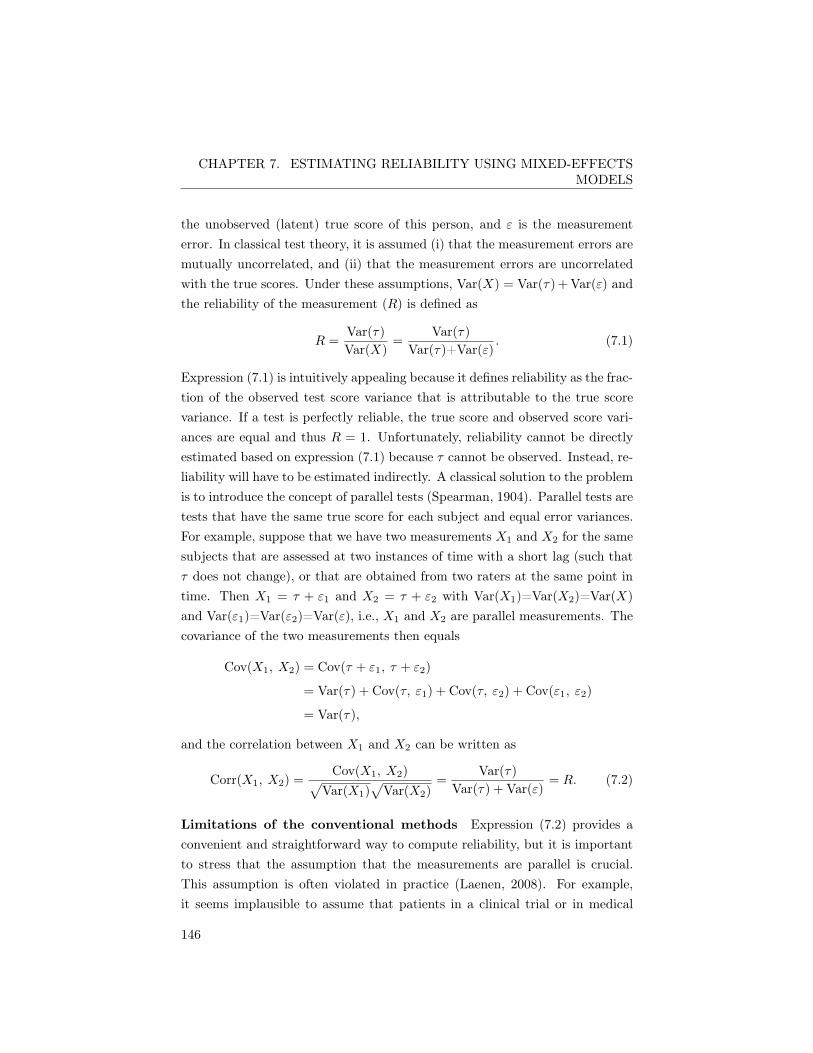
CHAPTER 7. ESTIMATING RELIABILITY USING MIXED-EFFECTSMODELS
the unobserved (latent) true score of this person, and " is the measurementerror. In classical test theory, it is assumed (i) that the measurement errors aremutually uncorrelated, and (ii) that the measurement errors are uncorrelatedwith the true scores. Under these assumptions, Var(X) = Var(⌧)+Var(") andthe reliability of the measurement (R) is defined as
R =
Var(⌧)Var(X)
=
Var(⌧)Var(⌧)+Var(")
. (7.1)
Expression (7.1) is intuitively appealing because it defines reliability as the frac-tion of the observed test score variance that is attributable to the true scorevariance. If a test is perfectly reliable, the true score and observed score vari-ances are equal and thus R = 1. Unfortunately, reliability cannot be directlyestimated based on expression (7.1) because ⌧ cannot be observed. Instead, re-liability will have to be estimated indirectly. A classical solution to the problemis to introduce the concept of parallel tests (Spearman, 1904). Parallel tests aretests that have the same true score for each subject and equal error variances.For example, suppose that we have two measurements X1 and X2 for the samesubjects that are assessed at two instances of time with a short lag (such that⌧ does not change), or that are obtained from two raters at the same point intime. Then X1 = ⌧ + "1 and X2 = ⌧ + "2 with Var(X1)=Var(X2)=Var(X)and Var("1)=Var("2)=Var("), i.e., X1 and X2 are parallel measurements. Thecovariance of the two measurements then equals
Cov(X1, X2) = Cov(⌧ + "1, ⌧ + "2)
= Var(⌧) + Cov(⌧, "1) + Cov(⌧, "2) + Cov("1, "2)
= Var(⌧),
and the correlation between X1 and X2 can be written as
Corr(X1, X2) =Cov(X1, X2)p
Var(X1)p
Var(X2)=
Var(⌧)Var(⌧) + Var(")
= R. (7.2)
Limitations of the conventional methods Expression (7.2) provides aconvenient and straightforward way to compute reliability, but it is importantto stress that the assumption that the measurements are parallel is crucial.This assumption is often violated in practice (Laenen, 2008). For example,it seems implausible to assume that patients in a clinical trial or in medical
146

CHAPTER 7. ESTIMATING RELIABILITY USING MIXED-EFFECTSMODELS
practice do not exhibit a systematic change over time as a result of their treat-ment. Another limitation of expression (7.2) is that only two measurementscan be considered, and these measurements should have the same test-retestinterval for all subjects. In practice, data may be available for more than twomeasurement moments and/or with different test-retest intervals. Further, theuse of expression (7.2) is less-than-ideal when data are missing, because sub-jects who have a missing observation for either X1 or X2 are discarded fromthe analysis. This approach does not only lead to a loss of information, butit also ignores the missing data generating mechanism. Basically, to obtainunbiased estimates for R using expression (7.2), the assumption that the dataare missing completely at random (MCAR) should be valid. This means thatthe missingness should not depend on the observed or the unobserved outcomes(Molenberghs and Kenward, 2007; Rubin, 1976). This is a strong and oftenunrealistic assumption, e.g., in a clinical trial setting it is conceivable that sub-jects who have lower scores at the first measurement in time (poorer health)are more likely to drop out of the study at the second measurement in time(missing value for X2).
7.2 Relevance of reliability
It is important to carefully consider the reliability of a measurement procedurein the context of designing a clinical trial. Indeed, even the most elegant studydesign will not overcome the damage that is caused by the use of unreliablemeasurement procedures (Fleiss, 1986). For example, biased sample selectionmay occur when patients are selected based on an unreliable measurement pro-cedure, and the sample size that is required to detect an important treatmentdifference (�) may increase substantially when the outcome of interest is quanti-fied using an unreliable measurement procedure. As an illustration of the latterissue, consider a situation where a t-test is used to evaluate the treatment effecton the primary endpoint in a clinical trial with two treatment groups. Whenthe measurement procedure that is used to quantify the primary endpoint hasperfect reliability (i.e., R = 1), the required sample size to detect � equals n⇤.However, when this measurement procedure has a less-than-perfect reliability(i.e., R < 1), the required sample size becomes n =
n⇤
R (for details, see Fleiss,1986). Thus, for example, when R = 0.50, the required sample size to detect
147

CHAPTER 7. ESTIMATING RELIABILITY USING MIXED-EFFECTSMODELS
� doubles compared to what would have been needed when R = 1. Clearly,an increase in the required sample size is an issue in nearly all clinical studies(e.g., increased study duration and cost), and it may even make the conductof the study infeasible (e.g., clinical trials in rare diseases).
7.3 Estimating reliability using the linear mixed-
effects model
A LMM can be written as
Yj = Xj� + Zjbj + "j , (7.3)
where Yj is the response vector for subject j (with j = 1, 2, ..., n subjects in thestudy), Xj and Zj are the known design matrices for the fixed- and random-effects, � is the vector that contains the fixed-effects, bj is the vector thatcontains the random-effects, and "j is the vector that contains the measurementerror (with bj ⇠ N (0, D) and "j ⇠ N (0, ⌃j), where D and ⌃j are generalvariance-covariance matrices). Model (7.3) thus assumes that the vector ofrepeated measurements for each subject follows a linear regression model wheresome of the parameters are population-specific (i.e., parameters that are thesame for all subjects in the population; the fixed-effects) and other parametersare subject-specific (i.e., parameters that differ for all subjects; the random-effects).
The residual component "j is often further decomposed as "j = "(1)j +
"(2)j . Here, "(2)j is a component of serial correlation and "(1)j is a componentof measurement error. Serial correlation results from the fact that within asubject, the (residuals of) observations that are closer in time are often ‘moresimilar’ (i.e., more strongly correlated) than observations that are more distantin time. It is assumed that "(1)j ⇠ N(0, �2Inj ) (with Inj an identity matrixof dimension nj = the number of repeated measurements in a subject) and"(2)j ⇠ N(0, ⌧2Hj) (with Hj the serial correlation matrix that only dependson j through the number of repeated measurements nj and the time pointsk and l at which the measurements are taken). The (k, l) element hjkl ofHj can then be modelled as hjkl = g (| tjk � tjl |) for a decreasing functiong. Two frequently used functions are the exponential and Gaussian correlation
148

CHAPTER 7. ESTIMATING RELIABILITY USING MIXED-EFFECTSMODELS
functions, defined as g (uk, l) = exp (��uk, l) and g (uk, l) = exp
⇣��u2
k, l
⌘,
respectively.
7.3.1 The mean structure of the model
Often, the average evolution of an endpoint over time can be reasonably wellmodelled using e.g., linear or quadratic polynomials. When this is not thecase, a more general family of parametric models that are based on so-calledfractional polynomial functions (Royston and Altman, 1994) can be used. Theidea is to fit regression models with m terms of the form tp, where the exponentsp are selected from a small predefined set S of both integer and non-integervalues. The linear predictor for a fractional polynomial of order M for covariatet (here: time) on the mean outcome is then defined as
�0 +
MX
m=1
�mtpm . (7.4)
Each power pm is chosen from a restricted set, typically S =
{�2, �1, �0.5, 0, 0.5, 1, 2, 3}. Note that when M = 2 and p1 = p2, thelinear predictor (7.4) becomes �0 + �1t
p1+ �2t
p1log(t). Also, when p = 0, this
is taken to refer to log(t) (Royston and Altman, 1994). In practice, all possiblemodels of degree 1 to M are fitted. Thus for M = 1, each of the 8 values of Sare used for the predictor tp1 , for M = 2 each of the 36 combinations of powersare used for the predictors tp1 and tp2 , and so on. Subsequently, the ‘best’fitting model is selected. This choice can be made in an informal way (i) basedon Akaike’s Information Criterion (AIC, where a lower value is indicative ofa better model fit) and/or (ii) by graphically evaluating the fit of the modelwith the observed data. The AIC adds the number of model parameters as apenalty to the log likelihood of the model, which may help to avoid over-fitting(even though one still may want to be careful not to select an overly complexmodel, in particular when a large number of candidate powers is considered).The main advantage of using fractional polynomials (rather than regular poly-nomials) is that they allow for a much more flexible parametrization, i.e., alarge number of different shapes of curves can be captured by even a relativelysmall M .
149

CHAPTER 7. ESTIMATING RELIABILITY USING MIXED-EFFECTSMODELS
7.3.2 The covariance structure of the model
Apart from the mean structure, the covariance structure of model (7.3) alsohas to be specified. Following Laenen (2008) and Vangeneugden et al. (2004),three different covariance structures can be considered. Model 1 is a randomintercept model, i.e., a LMM that only contains a random intercept in therandom part of the model
Yjk = µjk + b0j + "jk, (7.5)
where Yjk is the observed endpoint at measurement time k for subject j, µjk
is the mean as a function of the fixed-effects, b0j is the random intercept,and "jk is the residual. Based on this model, the reliability of the repeatedobservations taken at measurement times tl and tk can be estimated as (fordetails, see Laenen, 2008; Vangeneugden et al., 2004)
R (tk, tl) = R =
d
d+ �2, (7.6)
where d is the variance of the random intercept and �2 is the residual vari-ance. As can be seen in expression (7.6), the random intercept model assumesthat any two observations measured at different times have the same R. Thisassumption is often not realistic when repeated measures are considered, i.e.,measurements that are closer in time can be expected to be more stronglycorrelated than measurements that are more distant in time.
Therefore, Model 2 extends Model 1 by adding a serial correlation compon-ent
Yjk = µjk + b0j + "(1)jk + "(2)jk, (7.7)
where µjk, b0j are the same as in Model 1 and "(1)jk, "(2)jk are measurementerror and serial correlation components, respectively. Based on Model 2, thereliability of the repeated observations taken at measurement times tl and tk
can be estimated as (for details, see Laenen, 2008; Vangeneugden et al., 2004)
R (tk, tl) = R (ukl) =
d+ ⌧2 exp
✓�u2
lk
⇢2
◆
d+ ⌧2 + �2, (7.8)
where ukl = tl � tk, �2= Var
�"(1)j
�and ⌧2 = Var
�"(2)j
�. Model 2 thus no
longer assumes that R remains constant for all pairs of measurements. Instead,
150

CHAPTER 7. ESTIMATING RELIABILITY USING MIXED-EFFECTSMODELS
Table 7.1: Summary of the covariance structures used in Models 1–3, and theimpact on the estimated reliabilities.Model Estimated reliabilities R
Model 1: Random Intercept bR is identical for all pairs (tk, tl)
Model 2: Random intercept bR only depends on the time lag ukl = tl � tkand serial componentModel 3: Random intercept, bR is different for all pairs (tk, tl)slope, and serial component
Note. tk = measurement at time k.
it models R as a function of the time lag ukl between two measurements. Ascan be seen, a stronger serial effect (⇢2) leads to a faster decreasing R (ukl).
Finally, Model 3 further extends Model 2 by including a random slope formeasurement moment
Yjk = µjk + b0j + b1jtk + "(1)jk + "(2)jk, (7.9)
where µjk, b0j , "(1)jk, "(2)jk are the same as in Models 1 and 2, and b1j is therandom slope for measurement moment. Based on Model 3, the reliability ofthe repeated observations measured at times tl and tk can be estimated as (fordetails, see Laenen, 2008; Vangeneugden et al., 2004)
R (tk, tl) =
zkDz0
l + ⌧2 exp
✓�u2
kl
⇢2
◆
qzkDz
0k + ⌧2 + �2
qzlDz
0l + ⌧2 + �2
, (7.10)
where ukl = tl � tk, and zk, zl are the design rows in Z corresponding to timesk and l, respectively. As can be seen in expression (7.10), Model 3 no longerassumes that measurements taken at different time points but with the sametime lag have the same R. Instead, it provides estimates of reliability for allpairs of measurements.
Table 7.1 summarizes the covariance structures that are used in the differentmodels and their impact on the estimated R.
151

CHAPTER 7. ESTIMATING RELIABILITY USING MIXED-EFFECTSMODELS
7.3.3 Advantages of using linear mixed-effects models to
estimate reliability
As discussed above, LMMs can separate the mean and the variance structuresin the data. This has the advantage that the strong assumptions that areneeded to apply the conventional methods to estimate reliability can be relaxed(Laenen, 2008). Further, LMMs can deal with data structures where differentsubjects have a different number of repeated measurements (two or more),which may or may not be regularly spaced. Finally, LMMs are likelihood-based methods that provide valid results when the missingness mechanism ismissing at random (MAR) (Verbeke and Molenberghs, 2000). MAR meansthat the missingness may depend on the observed outcomes (e.g., the firstmeasurement X1) but not on unobserved outcomes. MAR is a substantiallyless restrictive assumption than MCAR, and is thus more likely to hold inpractice (Molenberghs and Kenward, 2007).
7.4 Case study: the cardiac output experiment
The data come from an experiment in which the cardiac output and strokevolume of N = 12 pigs was changed by increasing positive end-expiratorypressure levels (for details, see Section 2.1.4). The number of repeated ZSVmeasurements within an animal ranged between 9 and 47. Here, the reliabilityof ZSV is estimated.
The analyses below are conducted using the R package CorrMixed. In thecurrent section, only a summary of the main results is given and no referenceto the software is made. A more comprehensive analysis and step-by-stepinstructions on how the results can be obtained using the package is availablein the online Appendix Chapter 4. The online appendix can be downloaded athttps://dl.dropboxusercontent.com/u/8416806/PhD_Appendix.pdf.
7.4.1 Exploratory data analysis
Figure 7.1 shows the individual profiles (grey lines) of ZSV as a function ofmeasurement moment. As can be seen, there is substantial between- as well aswithin-animal variability. Further, drop-out is substantial, i.e., there are less
152

CHAPTER 7. ESTIMATING RELIABILITY USING MIXED-EFFECTSMODELS
observations at later measurement moments compared to the earlier measure-ment moments. This is more clearly depicted in Figure 7.2, where the numberof available observations at each of the different measurement moments areshown.
7.4.2 The mean structure of the model
Figure 7.1 shows that the average evolution over time (solid black line) ex-hibits a rather complex shape that cannot be modelled in a straightforwardway by using linear or quadratic polynomials. Therefore, fractional polyno-mials of order M = 1 to M = 5 were considered using the standard setS = {�2, �1, �0.5, 0, 0.5, 1, 2, 3} for the powers pm. Note that it is pos-sible to use a more extensive set of values for S if the original set does notprovide an adequate result, but the number of models that have to be fitted(and thus also the required computational time) increases sharply when thenumber of elements in S increases. For example, when the set S includes 8 ele-ments (the standard set), a total of 792 fractional polynomials of degree 5 canbe made. However, when the set S = {�3, �2.75, ..., 3} is used (25 elements),a total of 118, 755 fractional polynomials of degree 5 can be made. Similarly,M can be increased but this will again yield a sharp increase in the number ofmodels to be evaluated.
Thus, regression models that included linear predictors for fractional poly-nomials of maximum order M = 5 were fitted to the data of the case study.Table 7.2 shows the powers pm of the models of order 1 to 5 that had the lowestAIC values. As can be seen, the model with M = 3 had the lowest overall AICvalue. Figure 7.3 shows the predicted mean ZSV as a function of measurementmoment for this model.
Based on these results, the fractional polynomial of degree 3 was retainedas the ‘best’ model for the subsequent analyses. The relation between measure-ment point and the ZSV outcome was thus modelled as �1t3+�2t2+�3t2 log(t),and the LMMs further included an intercept, PEEP, and Cycle as fixed-effects.PEEP and Cycle were dummy-coded with 5 and 3 dummies, respectively.
153

CHAPTER 7. ESTIMATING RELIABILITY USING MIXED-EFFECTSMODELS
Table 7.2: The cardiac output experiment. Fractional polynomial results.M power pm AIC
1 �0.5 3788.703
2 0.5, 0.5 3786.096
3 2, 2, 3 3775.281
4 0.5, 1, 2, 2 3776.389
5 �2, �2, 0, 2, 3 3778.221
0 10 20 30 40
010
020
030
040
0
Time of measurement
ZSV
Figure 7.1: The cardiac output experiment. Individual profiles (grey lines)and mean values (black line) of the ZSV outcome as a function of time ofmeasurement.
154

CHAPTER 7. ESTIMATING RELIABILITY USING MIXED-EFFECTSMODELS
0 10 20 30 40
24
68
1012
Time of measurement
Num
ber o
f obs
erva
tions
Figure 7.2: The cardiac output experiment. Number of observations for theZSV outcome as a function of time of measurement.
155

CHAPTER 7. ESTIMATING RELIABILITY USING MIXED-EFFECTSMODELS
0 10 20 30 40
010
020
030
040
0
Time of measurement
Mea
n ZS
V
Figure 7.3: The cardiac output experiment. Observed means as a functionof time of measurement (solid line) and fitted fractional polynomial of degreeM = 3 (dashed line).
156

CHAPTER 7. ESTIMATING RELIABILITY USING MIXED-EFFECTSMODELS
7.4.3 The covariance structure
7.4.3.1 Model 1: random intercept model
When Model 1 was fitted to the data, it was obtained that bd = 1901.611 andb�2
= 2413.022, yielding bR = 0.441 (see expression (7.6)). A CI around bRcan be computed by using a (non-parametric) bootstrap or the Delta method(for details, see Appendix F). The bootstrap-based CI95% (using 500 bootstrapsamples) equalled [0.198; 0.618]. The Delta method-based CI95% was similarand largely overlapped, i.e., [0.189; 0.636]. Figure 7.4 (top left) illustrates theresults (the bootstrap-based CI is shown).
Overall, it can be concluded that bR is moderate and that there is substantialuncertainty in bR (which is not surprising given the small number of animals inthe study).
7.4.3.2 Model 2: random intercept and serial correlation
When Model 2 was fitted to the data, the estimated covariance parameterswere bd = 1349.650, b⌧2 = 2489.351, b⇢ = 3.581, and b�2
= 382.795. Thus,after correction for the fixed-effects, the covariance parameter estimates showedconsiderable remaining serial components.
Figure 7.4 (top right) shows the estimated R (ukl) (see expression (7.8))and their CI95% based on a bootstrap (the Delta method-based CIs were sim-ilar; data not shown). As can be seen, the estimated R were high for smalltime lags (e.g., bR (ukl = 0) = 0.865 and bR (ukl = 1) = 0.751) and subsequentlydecreased until they remained essentially constant at bR ⇡ 0.320 for measure-ments with time lags of about ukl = 10 and higher. It can also be observedthat the CI95% around R (ukl) were narrower for measurements with smallertime lags (e.g., for time lags ukl = 0 and ukl = 1, the CI95% = [0.817, 0.906]
and CI95% = [0.654, 0.836], respectively) and subsequently widened until theyremained stable around time lag ukl = 10 with CI95% = [0.045, 0.530].
157

CHAPTER 7. ESTIMATING RELIABILITY USING MIXED-EFFECTSMODELS
7.4.3.3 Model 3: random intercept, slope, and serial correlation
When Model 3 was fitted to the data, the estimated covariance parameterswere b⌧2 = 1952.970, b⇢ = 3.290, b�2
= 373.043, and
bD =
3219.869 �77.377
�77.377 3.686
!.
As noted earlier, based on Model 3 the estimated R (tl, tk) are different forall pairs of measurements (see expression (7.10)). Figure 7.4 (bottom) showsthe results graphically. In this figure, the utmost left line (marked with t1)depicts the estimated R (t1, tk), i.e., the estimated reliabilities of ZSV taken atmeasurement times 1 and 2–45. The line next to that one shows the estimatedR (t2, tk), etc. The figure shows that bR (tl, tk) is high when the time lag u issmall and flattens out for longer time lags. Further, depending on the particularpair of measurement moments (tl, tk) that is considered, the slope and amountof decline in bR (tl, tk) as a function of time lag differs. For example, whenconsidering bR (t1, tk), it can be seen that the estimated reliabilities declineparticularly strong for the first few subsequent measurements (say, until aboutt8) and continue to decline for all tk afterwards at a slower pace. Instead, forbR (t20, tk) there is only a substantial decline in the estimated reliabilities forthe first few subsequent measurements (say, until about t25) after which theestimated reliabilities remain essentially constant.
Based on Model 3, estimates of reliability are provided for each pair ofmeasurements, and the same obviously holds for the CIs. To avoid clutteredfigures, no CIs were added to Figure 7.4 (bottom). By means of illustration,Figure 7.5 provides the CI95% for R (t1, tk) (left) and R (t20, tk) (right). Ascan be seen, the CI95% increase as a function of time and tend to be wider forR (t20, tk) than for R (t1, tk) (as expected).
7.4.3.4 Selecting the most appropriate model
Based on the likelihood ratio (LR) test statistic G2, the fit of Models 1–3can be formally compared (for details, see Verbeke and Molenberghs, 2000).G2 is equal to �2 times the difference of the log likelihoods of the modelsbeing compared. Before discussing the results for the case study, some generalremarks are useful. First, when interest is in testing the need for including
158

CHAPTER 7. ESTIMATING RELIABILITY USING MIXED-EFFECTSMODELS
0 10 20 30 40
−0.5
0.0
0.5
1.0
Model 1
Time of measurement
Rel
iabi
lity
0 10 20 30 40
−0.5
0.0
0.5
1.0
Model 2
Time lag
Rel
iabi
lity
0 10 20 30 40
−0.5
0.0
0.5
1.0
Model 3
Time of measurement
Rel
iabi
lity
t1
Figure 7.4: The cardiac output experiment. Estimated reliabilities (solid lines)and 95% Confidence Intervals (dashed lines) for ZSV based on Model 1 (upperleft), Model 2 (upper right) and Model 3 (bottom). For Model 3, no Confid-ence Intervals are provided to avoid a cluttered figure. The utmost left linemarked with t1 depicts the estimated correlations between t1 and all othermeasurements, the line next to that one depicts the correlations between t2
and measurements 2–45, and so on.
159

CHAPTER 7. ESTIMATING RELIABILITY USING MIXED-EFFECTSMODELS
0 10 20 30 40
−1.0
−0.5
0.0
0.5
1.0
Estimated R(t1, tj)
Time of measurement
Rel
iabi
lity
0 10 20 30 40
−1.0
−0.5
0.0
0.5
1.0
Estimated R(t20, tj)
Time of measurement
Rel
iabi
lity
Figure 7.5: The cardiac output experiment. bR (t1, tk) (left) and bR (t20, tk)
(right) based on Model 3 and their 95% Confidence Intervals for the ZSVoutcome.
random effects in the model, the usual procedure where the test statistic G2
is compared to a �2 distribution with the number of degrees of freedom equalto the difference in the model parameters to be estimated is no longer valid.For example, consider the situation where interest is in testing whether one ortwo random effects are needed (Model 2 versus Model 3). This corresponds totesting that d12 = d21 = d22 = 0. To test this hypothesis, a mixture with equalweights 0.5 for �2
1 and �22 is needed (denoted by �2
1:2), because the variance d22
cannot be negative and thus the hypothesis test of interest is on the boundary ofthe parameter space (for details, see Verbeke and Molenberghs, 2000). Second,the results of the LR tests should be interpreted with caution because of thesmall sample size in the case study. Alternative testing procedures that arebased on permutation tests (see e.g., Lee and Braun, 2012) could provide amore viable alternative, but these methods are beyond the scope of the presentchapter. Third, the valid use of LR tests typically requires that the models arefitted using Maximum Likelihood estimation. The results provided above usedRestricted Maximum Likelihood (REML), but valid LR tests for comparingnested models with different covariance structures can still be obtained underREML estimation when the models that are compared have the same meanstructure (Verbeke and Molenberghs, 2000) – which was the case here, see
160

CHAPTER 7. ESTIMATING RELIABILITY USING MIXED-EFFECTSMODELS
Table 7.3: The cardiac output experiment. Fit indices of the different modelsfor the ZSV outcome.
# Pars. logL G2 Test p
Rand. Ser.
Model 1 1 0 �2328.910
Model 2 1 2 �2125.135 407.551 Model 2 vs. 1: �22 < 0.001
Model 3 3 2 �2121.399 7.472 Model 3 vs. 2: �21:2 0.015
Note. logL = log likelihood, G2 = �2 the difference of two log likelihoodvalues. Rand. = random effect parameters, ser. = serial components.
above.The log likelihood values for Models 1–3 are shown in Table 7.3. As can
be seen, the random intercept model with serial correlation (Model 2) fittedthe data significantly better than the random intercept model with no serialcorrelation (Model 1), p < 0.001. This test thus rejects the null hypothesis thatthere is no serial correlation process, i.e., it can be concluded that observationsthat are closer in time are stronger correlated than observations that are moredistant in time. Further, adding a random slope to the random intercept modelwith serial correlation (Model 3 versus Model 2) significantly improves themodel fit, p = 0.015 – though the gain was quite modest.
Model 3 is the model with the largest likelihood. It would be preferredif we would solely rely on statistical arguments. However, from an appliedperspective – i.e., also considering the practical usefulness of the results fora clinician or researcher – Model 2 is arguably to be preferred over Model 3because the former leads to reliability estimates that only depend on the timelag between two measurements. In contrast, Model 3 yields different reliabilityestimates for all possible pairs of measurements. Model 2 thus provides a muchmore parsimonious result compared to Model 3 – whilst the fit of both modelsis roughly comparable.
Further, even though Model 1 had a substantially poorer fit compared toModel 2, it still provides useful results for practitioners because it summarizesthe ‘overall’ reliability of a measurement procedure in a single parsimoniousindex.
161

CHAPTER 7. ESTIMATING RELIABILITY USING MIXED-EFFECTSMODELS
7.5 Discussion
The conventional methods to estimate reliability (e.g., the well-known Pearsoncorrelation coefficient) require assumptions that are often not met in real-lifestudies (e.g., parallel measurements, equally spaced test-retest intervals, etc.).The main aim of the current chapter was to illustrate how LMMs can be usedto estimate reliability in a flexible way. It was shown that this approach canbe successfully applied even in a ‘challenging’ dataset like in the presented casestudy – where the number of independent subjects is low, different subjectshave a different number of repeated observations, and several covariates haveto be taken into account. Overall, the analysis of the case study suggested thatthe reliability of ZSV was high (and its CIs narrow) when the time lag wassmall. For larger time lags, the reliability estimates decreased and their CIswidened.
Some critical remarks are in place. First, despite the major differencesbetween the conventional and the LMM-based methods to estimate reliability,there are also some obvious similarities. For example, the expressions to es-timate reliability based on Model 1 (see expression (7.6)) and the conventionalapproach (see expression (7.2)) are very similar (i.e., both are ratios of vari-ances). However, a fundamental difference between both methods is that theLMM-based approach does not require the parallel measurement assumption.The reason for this is that the mean and variance structures can be clearly sep-arated in LMMs (see above). For example, when the means at different timepoints are different (as was observed in the case study, see Figure 7.1), system-atic effects of time and other covariates can be taken into account by includingthem into the fixed-effect part of the model (as was done here). In essence,the main difference between the conventional and LMM-based approaches toestimate reliability is that the former requires a set of assumptions that aretaken care of in the study design, whereas the latter takes care of these as-sumptions through modelling at the analysis stage (Laenen, 2008). There ishowever a price to pay for the increased flexibility of the LMM-based approach,i.e., it requires substantially more complex statistical analyses compared to theconventional methods to estimate reliability. We tried to circumvent this issueby developing an R package (CorrMixed) that allows for obtaining reliabilityestimates based on Models 1–3 in a relatively straightforward way (for details,
162

CHAPTER 7. ESTIMATING RELIABILITY USING MIXED-EFFECTSMODELS
see the online Appendix Chapter 4).Second, in the present chapter the focus was entirely on the random effect
structure of the models because we were interested in estimating the reliabilityof the outcomes. Apart from estimating reliability, medical practitioners arealso often interested in obtaining so-called normative data. Normative data areused to convert a patient’s ‘raw’ outcomes into relative measures that reflectthe proportion of demographically-matched healthy controls in the populationwho have a lower outcome value compared to this patient. Such normative datafor repeated measurements can be obtained without any substantial additionaleffort using the same type of models that were fitted in the present chapter.The only difference is that the focus will then be on the fixed-effect part of themodel – rather than on the random effect structure (for details, see Van derElst et al., 2013).
Third, the outcome that was considered in the case study was a normallydistributed (Gaussian) variable. One may also be interested in estimating thereliability of repeated measurements of outcomes of a different distributionalnature, e.g., binary (yes/no, health/sick) or categorical ordered outcomes. Suchextensions are possible, but not trivial. The interested reader is referred toVangeneugden et al. (2010).
Fourth, in the analysis of the case study, the fixed-effect structures were keptconstant for Models 1 to 3 because we were primarily interested in evaluatingthe impact of different random-effect structures on the estimated reliabilities.Indeed, all models included PEEP (coded with 5 dummies), cycle (coded with3 dummies) and measurement moment (coded as a fractional polynomial oforder M = 3, i.e., �1t2 + �2t
2log(t) + �3t
3 with t = measurement moment) inthe fixed-effect part. The question may rise whether the results are sensitiveto the fixed-effect structure of the model. To evaluate this, the non-significantcovariates (using ↵ = 0.05) were excluded from the models based on a series oflikelihood ratio tests. Maximum likelihood (ML) was used to obtain the para-meter estimates of these models (rather than Restricted Maximum Likelihood),because valid classical likelihood ratio tests for the mean structure of nestedmodels can only be achieved with ML inference (Verbeke and Molenberghs,2000). The models that only include the significant covariates are referred toas the ‘reduced’ Models 1–3, whereas the models that include all covariatesare referred to as the ‘full’ Models 1–3. The sensitivity of the results for the
163

CHAPTER 7. ESTIMATING RELIABILITY USING MIXED-EFFECTSMODELS
mean structure of the model can then be evaluated by comparing the reliabilityestimates that are obtained based on the full and the reduced Models 1–3. Us-ing likelihood ratio tests (data not shown), it was established that the reducedModel 1 only included PEEP in the mean structure of the model. The reducedModel 2 was identical to the full model (i.e., all covariates in the full modelwere significant). The reduced Model 3 included Cycle and PEEP. Figure 7.6shows the estimated reliability coefficients based on the fitted full (left figures)and reduced (right figures) Models 1 (top figures) and 3 (bottom figures) res-ults. No results are shown for Model 2 because the full and the reduced modelwere identical. As can be seen, the results for the full and the reduced Models1 and 3 were similar. For example, for Model 1, bR = 0.441 (with 95% Confid-ence Interval [0.198; 0.618]) based on the full model and bR = 0.438 (with 95%
Confidence Interval [0.180; 0.600]) based on the reduced model. It can thusbe concluded that the estimated reliabilities are not strongly affected by thefixed-effect specification of the model, provided that the mean structure of themodel is supported by the data.
Finally, in the present chapter no time-varying covariates (other than meas-urement occasion itself) were considered, but depending on the study at handit may be useful to include such covariates. For example, consider a settingwhere one is interested in estimating the reliability of a psychiatric rating scalethat was scored by different physicians at the different measurement moments.When only a limited number of raters are involved in the study, the meth-odology that was proposed above can still be used in a straightforward way.Indeed, one can then simply include rater as a (dummy-coded) fixed-effect inthe mean structure of the model. On the other hand, when the number ofraters is large, it is more sensible to include rater in the random-effect part ofthe model.
164

CHAPTER 7. ESTIMATING RELIABILITY USING MIXED-EFFECTSMODELS
0 10 20 30 40
−0.5
0.0
0.5
1.0
Model 1, full fixed−effects structure
Time of measurement
Rel
iabi
lity
0 10 20 30 40
−0.5
0.0
0.5
1.0
Model 1, reduced fixed−effects structure
Time of measurement
Rel
iabi
lity
0 10 20 30 40
−0.5
0.0
0.5
1.0
Model 3, full fixed−effects structure
Time of measurement
Rel
iabi
lity
0 10 20 30 40
−0.5
0.0
0.5
1.0
Model 3, reduced fixed−effects structure
Time of measurement
Rel
iabi
lity
Figure 7.6: Estimated reliabilities (solid lines) and 95% bootstrap-based Con-fidence Intervals (dashed lines) for ZSV based on the ‘full’ (left figures) and the‘reduced’ (right figures) Model 1 (top figures) and Model 3 (bottom figures)results. The reliability estimates based on Model 3 do not include confidenceintervals to avoid cluttered figures.
165

CHAPTER 7. ESTIMATING RELIABILITY USING MIXED-EFFECTSMODELS
166

Appendices
167


Appendix A. Proof of Lemma 1.
Let us first consider the following diagram describing the association structurebetween the elements of the vector Y
0= (x, y, z).
In what follows it will be assumed that
Y =
0
BB@
x
y
z
1
CCA ⇠ N (0,⌃⇢) , where ⌃⇢ =
0
BB@
1 ⇢xy ⇢xz
⇢xy 1 ⇢yz
⇢xz ⇢yz 1
1
CCA .
Notice that, without loss of generality, it has been assumed that the componentsof Y have mean zero and variance one. This can be achieved by standardizationand will have no impact on statements regarding the association between thesecomponents. The question of interest is, given ⇢xy and ⇢xz, what can be saidabout the value of ⇢yz. The previous distributional assumptions imply that
y = ⇢xyx+ "y, "y ⇠ N�0, 1� ⇢2xy
�,
z = ⇢xzx+ "z, "z ⇠ N�0, 1� ⇢2xz
�,
with "y, "z ? x. Moreover,
⇢yz = cov(y, z) = cov(⇢xyx+ "y, ⇢xzx+ "z) = ⇢xy⇢xz + cov("y, "z).
Note further that cov("y, "z) = ⇢("y, "z)q(1� ⇢2xy)(1� ⇢2xz), and therefore
�
q(1� ⇢2xy)(1� ⇢2xz) cov("y, "z)
q(1� ⇢2xy)(1� ⇢2xz),
and the previous inequality leads to
⇢xy⇢xz �q(1� ⇢2xy)(1� ⇢2xz) ⇢yz ⇢xy⇢xz +
q(1� ⇢2xy)(1� ⇢2xz).
169

Using the previous expression and the causal diagrams
one gets
⇢S0S1⇢T1S1 �
q�1� ⇢2S0S1
� �1� ⇢2T1S1
� ⇢T1S0 ⇢S0S1⇢T1S1 +
q�1� ⇢2S0S1
� �1� ⇢2T1S1
�,
⇢S0S1⇢T0S0 �
q�1� ⇢2S0S1
� �1� ⇢2T0S0
� ⇢T0S1 ⇢S0S1⇢T0S0 +
q�1� ⇢2S0S1
� �1� ⇢2T0S0
�.
The previous inequalities imply
2⇢S0S1 �̄ �
q�1� ⇢2S0S1
� 2�̄c 2⇢S0S1 �̄ +
q�1� ⇢2S0S1
� ,
where = (⇢T0S0 , ⇢T1S1) =
q�1� ⇢2T0S0
�+
q�1� ⇢2T1S1
�and, consequently,
2�̄(1� ⇢S0S1)�
q�1� ⇢2S0S1
� 2(�̄ � �̄c) 2�̄(1� ⇢S0S1) +
q�1� ⇢2S0S1
� .
Finally, after dividing byp
(1� ⇢T0T1) (1� ⇢S0S1) one gets
2�̄
s1� ⇢S0S1
1� ⇢T0T1
�
s1 + ⇢S0S1
1� ⇢T0T1
2⇢� 2�̄
s1� ⇢S0S1
1� ⇢T0T1
+
s1 + ⇢S0S1
1� ⇢T0T1
.
Further assuming ⇢T0S0 = ⇢T1S1 = � one gets �̄ = � and = 2
p(1� �2) and
the previous inequality becomes
a� � bp(1� �2) ⇢� a� + b
p(1� �2),
or equivalently,|⇢� � a�| b
p(1� �2)
where a =
r1� ⇢S0S1
1� ⇢T0T1
and b =
r1 + ⇢S0S1
1� ⇢T0T1
.
170

Appendix B. Proving the expressions in Table 4.2.
In the following the expressions given in Table 4.2 (see page 73) will beformally deduced.
Case 1: P (�T = �S) = 1 Notice first that
P (�T = �S) =
1X
�1
P (�T = i,�S = i) =
1X
�1
⇡�ii = 1,
and, consequently, ⇡�ij = 0 for all i 6= j. It follows immediately that
AE = ⇡�11 � ⇡�
�1�1, AP = 1,
DE = 0, DP = 0,
CET = ⇡�11 � ⇡�
�1�1, R2H = 1.
The value of R2H follows from the theoretical properties outlined in Chapter 4
and Joe (1989). However, it may be instructive to compute it ‘manually’ inthese situations. To that end notice that, in this setting, ⇡�T
i = ⇡�Si = ⇡�
ii
and if one further considers 0 log 0 = limx!0 x log x = 0 then
I(�T,�S) =P1
i=�1 ⇡�ii log
✓⇡�ii
⇡�ii ⇡
�ii
◆= �
P1i=�1 ⇡
�ii log
�⇡�ii
�= H (�Tj) = H (�S) .
The previous expressions obviously imply R2H = 1.
Case 2: P (�T = ��S) = 1 Notice first that
P (�T = ��S) =
1X
�1
P (�T = i,�S = �i) =
1X
�1
⇡�i�i = 1,
and, hence, ⇡�ij = 0 for all i 6= �j. It follows immediately that
171

AE = ⇡�1�1 � ⇡�
�11, AP = 1,
DE = 0, DP = 0,
CET = ⇡�1�1 � ⇡�
�11, R2H = 1.
The value of R2H follows from the theoretical properties outlined in 4 and Joe
(1989) but it could also be calculated using arguments similar to the ones usedin Case 1.
Case 3: P��T = �S2
�= 1 Notice first that
P��T = �S2
�=
1X
�1
P��T = i2,�S = i
�= ⇡�
11 + ⇡�00 + ⇡�
1�1 = 1,
thus, only ⇡�11, ⇡�
00 and ⇡�1�1 are different from zero. It follows immediately that
AE = ⇡�11 + ⇡�
1�1, AP = 1,
DE = 0, DP = 0,
CET = ⇡�11 + ⇡�
1�1, R2H = 1.
The value of R2H follows from the theoretical properties outlined in 4 and
Joe (1989). However, it may be instructive to compute it ‘manually’ in thesesituations. To that end let us first calculate the mutual information betweenthe individual causal treatment effects
I(�T,�S) =⇡�11 log
"⇡�11
⇡�11
�⇡�11 + ⇡�
1�1
�#+ ⇡�
00 log
⇡�00
⇡�00⇡
�00
�+
⇡�1�1 log
"⇡�1�1
⇡�1�1
�⇡�11 + ⇡�
1�1
�#
=�
�⇡�11 + ⇡�
1�1
�log
�⇡�11 + ⇡�
1�1
�� ⇡�
00 log ⇡�00 = H(�T ).
Notice that here again it was assumed that 0 log 0 = limx!0 x log x = 0. Fur-
172

thermore, the entropy of �S can be computed as
H(�S) = �⇡�11 log ⇡
�11 � ⇡�
00 log ⇡�00 � ⇡�
1�1 log ⇡�1�1.
Finally, given that the logarithm is a monotonically increasing func-tion, one has that H(�T ) < H(�S). The previous inequality impliesmin [H(�T ), H(�S)] = H(�T ) and, consequently, R2
H = 1.
Case 4: P��T = �S2
� 1
�= 1 Notice first that
P��T = �S2
� 1
�=
1X
�1
P��T = i2 � 1,�S = i
�= ⇡�
0�1 + ⇡��10 + ⇡�
01 = 1,
and, hence, only ⇡�0�1, ⇡�
�10 and ⇡�01 are different from zero. It follows imme-
diately thatAE = 0, AP = 0,
DE = �⇡�10, DP = 1,
CET = �⇡�10, R2H = 1.
The value of R2H follows from the theoretical properties outlined in 4 and Joe
(1989) but it could also be calculated using arguments similar to the ones usedin Case 3.
Case 5: �T?�S Notice first that, in this setting, ⇡�ij = ⇡�T
i ⇡�Sj and,
therefore,
AE =⇡�T1 ⇡�S
1 � ⇡�T�1 ⇡
�S1 + ⇡�T
1 ⇡�S�1 � ⇡�T
�1 ⇡�S�1
=
�⇡�S1 + ⇡�S
�1
� �⇡�T1 � ⇡�T
�1
�
=
�1� ⇡�S
0
� �⇡�T1 � ⇡�T
�1
�.
173

Furthermore,
DE =⇡�T1 ⇡�S
0 � ⇡�T�1 ⇡
�S0 = ⇡�S
0
�⇡�T1 � ⇡�T
�1
�
CET =⇡�T1 � ⇡�T
�1 .
It immediately follows thatAE =
�1� ⇡�S
0
� �⇡�T1 � ⇡�T
�1
�, AP = 1� ⇡�S
0 ,
DE = ⇡�S0
�⇡�T1 � ⇡�T
�1
�, DP = ⇡�S
0 ,
CET = ⇡�T1 � ⇡�T
�1 , R2H = 0.
The value of R2H follows from the theoretical properties outlined in Chapter
4 and Joe (1989) but it is also a direct consequence of the expression for themutual information.
174
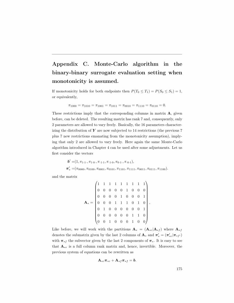
Appendix C. Monte-Carlo algorithm in the
binary-binary surrogate evaluation setting when
monotonicity is assumed.
If monotonicity holds for both endpoints then P (T0 T1) = P (S0 S1) = 1,or equivalently,
⇡1000 = ⇡1010 = ⇡1001 = ⇡1011 = ⇡0010 = ⇡1110 = ⇡0110 = 0.
These restrictions imply that the corresponding columns in matrix A, givenbefore, can be deleted. The resulting matrix has rank 7 and, consequently, only2 parameters are allowed to vary freely. Basically, the 16 parameters character-izing the distribution of Y are now subjected to 14 restrictions (the previous 7plus 7 new restrictions emanating from the monotonicity assumption), imply-ing that only 2 are allowed to vary freely. Here again the same Monte-Carloalgorithm introduced in Chapter 4 can be used after some adjustments. Let usfirst consider the vectors
b
0=(1,⇡1·1·,⇡1·0·,⇡·1·1,⇡·1·0,⇡0·1·,⇡·0·1),
⇡
0⇤ =(⇡0000,⇡0100,⇡0001,⇡0101,⇡1101,⇡1111,⇡0011,⇡0111,⇡1100).
and the matrix
A⇤ =
0
BBBBBBBBBBBBB@
1 1 1 1 1 1 1 1 1
0 0 0 0 0 1 0 0 0
0 0 0 0 1 0 0 0 1
0 0 0 1 1 1 0 1 0
0 1 0 0 0 0 0 0 1
0 0 0 0 0 0 1 1 0
0 0 1 0 0 0 1 0 0
1
CCCCCCCCCCCCCA
,
Like before, we will work with the partitions A⇤ = (A⇤r|A⇤f ) where A⇤f
denotes the submatrix given by the last 2 columns of A⇤ and ⇡0⇤ = (⇡
0⇤r|⇡⇤f 0
)
with ⇡⇤f the subvector given by the last 2 components of ⇡⇤. It is easy to seethat A⇤r is a full column rank matrix and, hence, invertible. Moreover, theprevious system of equations can be rewritten as
A⇤r⇡⇤r + A⇤f⇡⇤f = b.
175

Based on the previous developments the following version of the original al-gorithm can then be used
1. Select a grid of values G = {g1, g2, ..., gK} in (0, 1).
2. From k = 1 till K do
(a) Using the Randfixedsum algorithm, generate the 2 components of⇡⇤f uniformity on the line 10
⇡⇤f = gi.
(b) Calculate ⇡⇤r = A�1⇤r (b� A⇤f⇡⇤f ) and ⇡0
⇤ =
⇣⇡
0⇤r|⇡
0⇤f
⌘.
(c) Repeat steps 2a and 2b M times.
3. From these K ⇥M ⇡⇤ vectors select those with all components positive(the valid vectors ⇡⇤ > 0).
If monotonicity is assumed for only one endpoint then a similar strategy canbe followed.
176

Appendix D. Proof of Lemma 3.
Let us consider a general function : {�1, 0, 1} ! {�1, 0, 1}, we want to findthe function b that maximizes the probability
P [�T = (�S)] =
1X
i=�1
P (�T = i, (�S) = i) ,
=
1X
i=�1
X
j2 �1(i)
P (�T = i,�S = j) ,
=
1X
i=�1
X
j2 �1(i)
P (�T = i|�S = j)P (�S = j) ,
where �1(i) : {j 2 {�1, 0, 1} : (j) = i}. If P (�S = j) = 0 then
P (�T = i|�S = j) does not contribute to the probability P [�T = (�S)]
and, hence, one can focus only on the support of S. Without loss of general-ity, let us assume that P (�S = j) > 0 for all j. Basically, can be thoughtof as a correspondence between the column numbers and the row numbers ofthe distribution of �, i.e., between the column and row numbers of Table 4.1,where every column number j gets mapped into one and only one row numberi. Therefore, defining a function is equivalent to choosing 3 cells in Table4.1, each of them located in a different column. Consequently, maximizingP [�T = (�S)] is equivalent to maximizing the sum of the corresponding cellsprobabilities in each column or, in other words, maximizing P (�T = i|�S = j)
for j = �1, 0, 1 and, thus,
b(j) = arg max
ir(i, j) = arg max
iP (�T = i|�S = j) .
177

Appendix E. Proof of Lemma’s 4–5.
Proof of Lemma 4. In the following Lemma 4 will be proven.
1. R2 is invariant by bijective transformations of �T and S
The result follows from the fact that the mutual information I (�Tj ,S) isinvariant by bijective transformations of �T and S.
2. 0 R2 1
It is a direct consequence of R2 = maxt
hcorr
⇣�Tj , t
0S
⌘i2.
3. R2 = 0 if and only if �T0Sr = �T1Sr for all r = 1, 2 . . . p
Given that ⌃�1SS is positive-definite it follows from expression (4) in the
manuscript that R2 = 0 if and only if a1⌃TS = 0. Moreover a1⌃TS = 0 if and
only if �T0Sr = �T1Sr for all r = 1, 2 . . . p. Obviously, under homoscedasticity�T0Sr = �T1Sr for all r if and only if ⇢T0Sr = ⇢T1Sr for all r.
4. R2 = 1 if and only if there exists a deterministic relationship between �T
and S.From R2
= maxt
hcorr
⇣�Tj , t
0S
⌘i2it is clear that R2
= 1 if and only ifthere exists a t⇤.
Proof of Lemma 5. In the following Lemma 5 will be proven.
Notice that for every vector t 2 Rp there exists a t0 = (t, 0)0 2 Rp+1
so that corr⇣�Tj , t
0S
⌘= corr
⇣�Tj , t
0
0S⇤
⌘. Consequently,
R2 = max
t2Rp [corr (�Tj , t0§)]
2= max
t02Rp+1 [corr (�Tj , t00§⇤)]
2 max
t⇤2Rp+1 [corr (�Tj , t0⇤§⇤)]
2= R2
⇤
Proof of Lemma 6. In the following Lemma 6 will be proven.
To that end let us consider the following two cases
178

Case 1: Z = 0
T =�0 +
pX
k=1
↵kSk + ",
cov(T, Sr) = �T0Sr =
pX
k=1
↵kcov(Sk, Sr) =
pX
k=1
↵k�SkSr,
for all r = 1, 2 . . . p. Notice that to obtain the previous expression it wasassumed that Z?Sr for all r. Due to randomization, the assumption ofindependence Z?Sr will be often valid for any pretreatment predictor in aclinical trial context.
Case 2: Z = 1
T =�0 + �1 +
pX
k=1
↵kSk + ",
cov(T, Sr) = �T1Sr =
pX
k=1
(↵k + �k)cov(Sk, Sr),
=
pX
k=1
↵k�SkSr +
pX
k=1
�k�SkSr.
From cases 1 and 2 one has �T1Sr ��T0Sr =
Ppk=1 �k�SkSr for all r = 1, 2 . . . p.
This expressions conform a system of p linear equations in p covariatesthat can be rewritten in matrix form as a1⌃TS = �
0⌃SS and has solution�
0= a1⌃TS⌃
�1SS or, equivalently, � = ⌃�1
SS⌃STa01. Substituting this value in
expression 5.4 in the main thesis text leads to
R2 =
a1⌃TS�
��T=
a1⌃TS⌃�1SS⌃SS�
��T=
�
0⌃SS�
��T.
179

Appendix F. Delta-method based confidence in-
tervals for reliability.
When the most general model is considered (Model 3, see Section 7.3), then
R =
ZsDZ0
t + ⌧2 (Hi)stpZsDZ0
s + ⌧2 + �2pZtDZ
0t + ⌧2 + �2
,
with all components as defined in Chapter 7 and D =
d11 d12
d21 d22
!.
Letf (Z1, Z2, h, k) = Z1DZ
0
2 + ⌧2h+ �2k,
then
R = f (Zs, Zt, (Hi)st , 0) · f (Zs, Zs, 1, 1)�1/2
· f (Zt, Zt, 1, 1)�1/2
= g1 · g2 · g3
= f1 · f�1/22 · f
�1/23 .
Further,@R
@↵=
@g1@↵
· g2 · g3 + g1@g2@↵
g3 + g1 · g2@g3@↵
=
@f1@↵
· f�1/22 · f
�1/23 + f1
⇣�
12f
�3/22
⌘ @f2@↵
· f�1/23 + f1 · f
�1/22
⇣�
12f
�3/23
⌘ @f3@↵
,
with ↵ =
0
BBBBBBBBBB@
d11
d21
d12
d22
⌧2
�2
1
CCCCCCCCCCA
.
@f
@dl= Z1DlZ
0
2, with
180

D(11) =
1 0
0 0
!, D(12) =
0 1
1 0
!, D(22) =
0 0
0 1
!.
@f
@⌧2= h
@f
@�2= k
var⇣bR⌘⇠
=
✓@R
@↵
◆0
var(↵)@R
@↵.
The var(↵) can be obtained in e.g. SAS by using the asycov option in thePROC MIXED call.
181

182

Summary
It is sometimes not feasible to use the true endpoint (i.e., the most credibleindicator of the therapeutic response) in a clinical trial. For example, the trueendpoint may require a long follow-up time (e.g., survival time in oncology)and thus it would take a long time to evaluate the new therapy using thisendpoint. In such a situation, it can be an appealing strategy to substitute thetrue endpoint by another endpoint that can be measured earlier (e.g., changein tumour volume in oncology) and that can predict the treatment effect on thetrue endpoint. Such a replacement outcome for the true endpoint is referredto as a ‘surrogate endpoint’.
Before the candidate surrogate endpoint can replace the true endpoint, ithas to be formally evaluated. This is not a trivial task, and over the last decadesa number of statistical procedures to achieve this aim have been proposed.These methods can be classified along two dimensions, taking into account(i) whether they use information from a single or from multiple clinical trials,and (ii) whether they focus on individual or on expected causal effects. Whenthe focus is on individual causal effects, it is assumed that each patient j hastwo potential outcomes for the true endpoint T : an outcome T0j that wouldbe observed under the control treatment and an outcome T1j that would beobserved under the experimental treatment – and similarly for S. These arecalled ‘potential outcomes’, because they represent the outcomes that couldhave been observed if the patient had received the control treatment or theexperimental treatment. Individual causal effects can then be defined as �Tj =
T1j � T0j and �Sj = S1j � S0j . Expected causal treatment effects essentiallyrefer to the averaged individual causal treatment effects.
In Chapter 3, the conceptual frameworks that underlie the surrogate evalu-
183

ation methodology based on individual and expected causal effects in the single-and the multiple-trial settings is detailed for scenarios where both endpointsare normally distributed variables. Even though the causal inference paradigmis typically framed into the single-trial setting, it is shown that this methodo-logy can also be embedded in the multiple-trial setting. Further, new metricsof surrogacy based on individual causal effects in the single and multiple trialsettings are proposed – the so-called individual and meta-analytic individualcausal associations, respectively. Both metrics essentially quantify the accuracyby which the individual causal treatment effect on T can be predicted basedon the individual causal treatment effect on S. Simulation studies showed thatthe metrics of surrogacy based on individual and expected causal effects wererelated, but in a rather complex way.
In Chapter 4, the focus is on a surrogate evaluation scenario in the singletrial setting where both endpoints are binary. Two new metrics of surrogacybased on individual causal effects are proposed. Similarly to what is the casein the normal-normal scenario, the individual causal association quantifies theoverall accuracy by which the individual causal treatment effect on T can bepredicted based on the individual causal treatment effect on S. It has anappealing interpretation in terms of uncertainty reduction in the prediction of�Tj based on �Sj . The so-called ‘surrogate predictive function’ supplementsthis metric in the sense that it allows for a more fine-grained assessment of how�Tj and �Sj are related. This function basically allows us to determine whatthe most likely outcome of �Tj will be for a given outcome of �Sj . In this wayit allows for the evaluation of some important scientific questions that cannotbe explicitly addressed using the individual causal association. For example onemay be interested in quantifying the conditional probability that the treatmenthas a negative impact on T given that the treatment has a beneficial impact onS (i.e., the probability that the surrogate will produce a false positive result).
Several other topics that are related to surrogate evaluation methods arediscussed in the second part of this thesis. In Chapter 5, the focus is on‘personalized medicine’. Personalized medicine refers to the idea that a medicaltreatment should be tailored to the individual patients’ specific characteristics,as opposed to the practice where all patients who have the same disease receivethe same treatment (i.e., the treatment that works best ‘on average’ in thepopulation). It is argued that the commonly used correlational approaches to
184

identify predictors of treatment success are not sufficient to answer the relevantscientific question. A new metric that quantifies the extent to which therapeuticsuccess can be predicted based on pretreatment predictors is proposed, the so-called predictive causal association.
In the meta-analytic surrogate evaluation framework (which assesses sur-rogacy based on expected causal effects in a multi-trial setting), linear mixed-effects models are typically fitted to estimate the surrogacy metrics of interest.Unfortunately, in real-life surrogate evaluation settings, model convergenceproblems are prevalent. In Chapter 6, simulation studies are used to exam-ine the factors that affect model convergence and a multiple imputation-basedapproach to reduce model convergence issues is proposed.
In the meta-analytic surrogate evaluation approach, one of the metrics thatassesses surrogacy is the coefficient of individual-level surrogacy. This met-ric essentially quantifies the treatment- and trial-corrected correlation betweenS and T . A psychometric concept that is closely related to individual-levelsurrogacy is reliability. Reliability quantifies the reproducibility (or, predict-ability) of two or more outcomes that are repeatedly measured within the sameperson. In Chapter 7, some methods are proposed to estimate reliability in aflexible way using linear mixed-effects models.
The methodology that was developed in this thesis has been implemen-ted in three R packages, i.e., the Surrogate, EffectTreat, and CorrMixed pack-ages (available for download at CRAN). A detailed account on how the res-ults of the case study analyses that are described throughout this thesiscan be replicated using these R packages is available in an online Appendixthat accompanies this thesis. The online appendix can be downloaded athttps://dl.dropboxusercontent.com/u/8416806/PhD_Appendix.pdf.
185

186

Samenvatting
In klinische studies is het niet altijd mogelijk om de meest relevante indicatorvan behandelingssucces te gebruiken. Zo bestaat bijvoorbeeld de mogelijkheiddat het klinische eindpunt pas lange tijd na de start van de studie kan wordengemeten (bvb. overlevingstijd in oncologie). Gebruik van dit klinisch eindpuntzou dan ook impliceren dat de nieuwe behandeling pas na een lange tijd kanworden geëvalueerd. Als zulke situatie zich voordoet kan het interessant zijnom het klinisch eindpunt te vervangen door een zgn. ‘surrogaat eindpunt’. Ditis een eindpunt dat sneller kan worden gemeten dan het klinisch eindpunt, endat toelaat om het effect van de behandeling op het klinisch eindpunt accuraatte schatten. Een mogelijke surrogaat voor overlevingstijd in oncologie zou bvb.verandering van tumorvolume kunnen zijn.
Alvorens een klinisch eindpunt (K) kan worden vervangen door een surrog-aat eindpunt (S) is het noodzakelijk om empirisch te verifiëeren dat S hiervoor‘geschikt’ is, i.e., dat S toelaat om het effect van de behandeling op K ac-curaat in te schatten. De laatste 40 jaar zijn een groot aantal statistischeprocedures ontwikkeld om na te gaan of een kandidaat S werkelijk geschikt isom K te vervangen. Deze methoden verschillen m.b.t. twee belangrijke aspec-ten: (i) sommige methoden nemen aan dat de data van één klinische studiebeschikbaar is terwijl andere methoden aannemen dat de data van meerdereklinische studies beschikbaar zijn, en (ii) sommige methoden focussen op indi-viduele causale effecten terwijl andere methoden focussen op verwachtte causaleeffecten. Als de focus op individuele causale effecten ligt, wordt aangenomendat elke patiënt j twee mogelijke uitkomsten heeft voor K: een waarde K0j
die zou worden geobserveerd als de patiënt de controlebehandeling krijgt, eneen waarde K1j die zou worden geobserveerd als de patiënt de experimentele
187

behandeling krijgt (en idem voor S). Individuele causale effecten worden dangedefiniëerd als �Kj = K1j �K0j en �Sj = S1j � S0j .
In Hoofdstuk 3 worden de theoretische kaders besproken die gebruiktworden om surrogaten te evalueren op basis van individuele en verwachttecausale effecten in settings waar de data van één en meerdere klinische studiesbeschikbaar zijn. Er worden nieuwe indices voorgesteld die de accuraatheidvan een kandidaat S om K te voorspellen kwantificeren. Daarnaast wordenook simulatiestudies uitgevoerd, die aantonen dat surrogaat-indices gebaseerdop individuele en verwachtte causale effecten aan mekaar gerelateerd zijn.
Hoofdstuk 4 gaat dieper in op scenarios waar zowel S als K binaire uitkom-sten zijn. Twee nieuwe surrogaat-indices worden voorgesteld. Een eerste maat,de ‘individuele causale associatie’ kwantificeert de accuraatheid waarmee hetindividuele causale behandelingseffect op K kan worden voorspeld op basis vanhet individuele causale behandelingseffect op S. Een tweede maat, de ‘surrog-aat predictieve functie’ laat toe om op een meer fijnmazige manier de relatietussen �Kj en �Sj te bestuderen, i.c., om de meest waarschijnlijke uitkomstvoor �Kj gegeven �Sj te bekijken. Dit laat toe om belangrijke wetenschap-pelijke vragen te beantwoorden, bvb. de vraag hoe waarschijnlijk het is datde behandeling een negative impact op K zal hebben als de behandeling eenpositieve impact heeft op S, i.c., de waarschijnlijkheid dat de surrogaat eenvals-positief resultaat zal opleveren.
Diverse andere onderwerpen die gerelateerd zijn aan de evaluatie van sur-rogaten worden besproken in het tweede deel van deze thesis. In Hoofdstuk 5ligt de focus op ‘gepersonaliseerde geneeskunde’. Dit concept verwijst naar hetidee dat een behandeling idealitair op maat van de individuele patiënt zou mo-eten worden aangeboden, in tegenstelling tot het huidige dominante paradigmain de geneeskunde, waar alle patiënten met eenzelfde ziekte ook dezelfde behan-deling krijgen (i.c., de behandeling die ‘gemiddeld genomen’ het beste werktin de populatie). De huidige methoden die gebruikt worden om predictorenvan behandelingssucces op te sporen zijn gebaseerd op correlationele model-len. In hoofdstuk 5 wordt een alternatieve aanpak voorgesteld gebaseerd opindividuele causale modellen.
In situaties waar surrogaten moeten worden gëevalueerd op basis van meer-dere klinische studies (de zgn. ‘meta-analytische setting’) worden vaak mixed-effects modellen gebruikt om surrogacy te kwantificeren. Het fitten van dit
188

soort modellen is vaak niet evident, en convergentieproblemen komen frequentvoor. In Hoofdstuk 6 worden simulatiestudies gebruikt om na te gaan welkefactoren een invloed habben op de convergentie van de modellen. Er wordtook een methode die gebasseerd is op meervoudige imputatie voorgesteld omde convergentieproblemen te vermijden.
In de meta-analytische setting wordt de correlatie tussen S and K (gecorri-geerd voor mogelijke trial- en behandelingseffecten) vaakt gebruikt om de kwal-iteit van een kandidaat surrogaat te kwantificeren. Een psychometrisch conceptdat hieraan nauw aansluit is betrouwbaarheid. Betrouwbaarheid kwantificeertde herhaalbaarheid van twee of meer metingen binnen dezelde persoon. InHoofdstuk 7 worden enkele methoden voorgesteld om betrouwbaarheid op eenflexibele manier te schatten gebaseerd op mixed-effects modellen.
De methodologie die werd ontwikkeld in deze thesis is geïmplementeerdin drie R pakketten (i.c., de Surrogate, EffectTreat, en CorrMixed pakketten)die kunnen worden gedownload via CRAN. Alle voorbeeldanalyses die wordenbeschreven in deze thesis kunnen worden gerepliceerd met deze R pakketten.Meer details over hoe deze analyses kunnen worden uitgevoerd zijn te vinden ineen online Appendix, zie https://dl.dropboxusercontent.com/u/8416806/PhD_Appendix.pdf.
189

190

Bibliography
Alonso, A., and Van der Elst, W. (2016). Surrogate markers validation: Thecontinuous-binary setting from a causal inference perspective. Technical re-port.
Alonso, A., and Molenberghs, G. (2007). Surrogate marker evaluation from aninformation theoretic perspective. Biometrics, 63, 180–186.
Alonso, A., Van der Elst, W., Molenberghs, G., Buyse, M., and Burzykowski, T.(2015). On the relationship between the causal-inference and meta-analyticparadigms for the validation of surrogate endpoints. Biometrics, 71, 15–24.
Alonso, A. A., Bigirumurame, T., Burzykowski, T., Buyse, M., Molenberghs,G., Muchene, L., Perualila, N. J., Shkedy, Z., and Van der Elst, W. (2016).Applied surrogate endpoint evaluation methods with SAS and R.
Abrahams, E., and Silver, M. (2010). The History of Personalized Medicine. InE. Gordon and S. Koslow (Eds.), Integrative Neuroscience and PersonalizedMedicine, pp. 3-16. New York, NY: Oxford University Press.
American Psychiatric Association (2000). Diagnostic and Statistical Manual ofMental Diseases. Washington, DC: American Psychiatric Association.
Baker S. G., and Kramer B. S. (2015). Evaluating surrogate endpoints, pro-gnostic markers, and predictive markers: some simple themes. Clinical Trials,12, 299–308.
Banerjee, P., Choi, B., Shahine, L. K., Jun, S. H., O’Leary, K., Lathi, R. B.,Westphal, L. M., Wong, W. H., and Yao, M. W. (2010). Deep phenotyping
191

BIBLIOGRAPHY
to predict live birth outcomes in in vitro fertilization. Proceedings of theNational Academy of Sciences, 107, 13570–13575.
Burzykowski, T., Molenberghs, G., and Buyse, M. (2005). The Evaluation ofSurrogate Endpoints. New York: Springer-Verlag.
Buyse, M., and Molenberghs, G. (1998) The validation of surrogate endpointsin randomized experiments. Biometrics, 54, 1014–1029.
Buyse, M., Molenberghs, G., Burzykowski, T., Renard, D., and Geys, H.(2000). The validation of surrogate endpoints in meta-analyses of randomizedexperiments. Biostatistics, 1, 49–67.
Brockett, P. L., Charnes, A., and Cooper, W. W. (1980). MDI estimation viaunconstrained convex programming. Communications in Statistics, 9, 223–234.
The Cardiac Arrhythmia Suppression Trial Investigators (1989). PreliminaryReport: Effect of Encainide and Flecainide on Mortality in a RandomizedTrial of Arrhythmia Suppression after Myocardial Infarction. The New Eng-land Journal of Medicine, 321, 406-412.
Carpenter, J., and Kenward, M. G. (2014). Multiple Imputation and its Ap-plication. New York: John Wiley & Sons.
Conlon, A. S., Taylor, J. M. G., and Elliott, M. R. (2014). Surrogacy assess-ment using principal stratification when surrogate and outcome measures aremultivariate normal. Biostatistics, 15, 266–283.
Cortiñas Abrahantes, J., Molenberghs, G., Burzykowski, T., Shkedy, Z., andRenard D. (2004). Choice of units of analysis and modeling strategies inmultilevel hierarchical models. Computational Statistics and Data Analysis,47, 537–563.
Cortiñas Abrahantes, J., Shkedy, Z., and Molenberghs, G. (2004). Alternativemethods to evaluate trial-level surrogacy. Clinical Trials, 5, 194–208.
Daniels, M. J., and Hughes, M. D. (1997). Meta-analysis for the evaluation ofpotential surrogate markers. Statistics in Medicine, 16, 1515–1527.
192

BIBLIOGRAPHY
Daniels, M. J., Roy, J. A., Kim, C., Hogan, J. W., and Perri, M. G. (2012).Bayesian inference for the causal effect of mediation. Biometrics, 68, 1028–1036.
Dempster, A. P., Laird, N. M., and Rubin, D. B. (1977). Maximum likelihoodfrom incomplete data via the EM algorithm (with discussion). Journal of theRoyal Statistical Society Series B, 39, 1–38.
Edwin, T. J. (1982). On the rationale of maximum-entropy methods. Proceed-ings of the IEEE, 70, 939–952.
Elliott, M. R., Li, Y., and Taylor, J. M. G. (2013). Accommodating missingnesswhen assessing surrogacy via principal stratification. Clinical Trials, 10, 363–377.
Emberson, P., Stafford, R., and Davis, R. (2010). Techniques for the synthesisof multiprocessor tasksets. Paper presented at 1st International Workshopon Analysis Tools and Methodologies for Embedded and Real-time Systems,Brussels, July 6th, 6–11.
FDA (2013). Paving the way personalized medicine: FDA’s role in a new eraof medical product development. Retrieved fromhttp://www.fda.gov/downloads/ScienceResearch/SpecialTopics/PersonalizedMedicine/UCM372421.pdf
Fleiss, J. L. (1986). Design and analysis of clinical experiments. Wiley: NewYork.
Fleming, T. R., and DeMets, D. L. (1996). Surrogate end points in clinicaltrials: Are we being misled? Annals of Internal Medicine, 125, 605–613.
Frangakis, C. E., and Rubin, D. B. (2002). Principal stratification in causalinference. Biometrics, 58, 21–29.
Freedman, L. S. (2001). Confidence intervals and statistical power of the ‘valid-ation’ ratio for surrogate and intermediate endpoints. Journal of StatisticalPlanning and Inference, 96, 143–153.
Freedman. L. S., Graubard, B. I., and Schatzkin, A. (1992). Statistical valid-ation of intermediate endpoints for chronic diseases. Statistics in Medicine,11, 167–178.
193

BIBLIOGRAPHY
Gail, M. H., Pfeiffer, R., van Houwelingen, H. C., and Carroll, R. J. (2000). Onmeta-analytic assessment of surrogate outcomes. Biostatistics, 1, 231–246.
Gelman, A., and Hill, J. (2006). Data Analysis Using Regression and Multi-level/Hierarchical Models. Cambridge University Press.
Geys, H (2005). Validation using single-trial data: mixed binary and continuousoutcomes. In T. Burzykowski, G. Molenberghs, and M. Buyse (Eds.), Theevaluation of surrogate endpoints, (pp. 83–93). New York: Springer-Verlag.
Gilbert, P. B., and Hudgens, M. G. (2008). Evaluating candidate principalsurrogate endpoints. Biometrics, 64, 1146–1154.
Guy, W. (1976). Clinical Global Impression. In ECDEU assessment manual forpsychopharmacology (revised), (pp. 217–221). National Institute of MentalHealth.
Holland, P. W. (1986). Statistics and Causal Inference. Journal of the AmericanStatistical Association, 81, 945–960.
Jaynes, E. T. (1985). Where do we go from here? In C. R. Smith and J.W. T. Grandy (Eds.), Maximum-Entropy and Bayesian Methods in InverseProblems, pp. 21–58. Kluwer Academic Publishers.
Joe, H. (1989). Relative entropy measures of multivariate dependence. Journalof the American Statistical Association, 84, 157–164.
Joffe, M. M., and Greene, T. (2009). Related causal frameworks for surrogateoutcomes. Biometrics, 65, 530–538.
Kane, J., Honigfeld, G., Singer, J., and Meltzer, H. (1988). Clozapine for thetreatment-resistant schizophrenic. A double-blind comparison with chlorpro-mazine. Archives of General Psychiatry, 45, 789–796.
Laenen, A. (2008). Psychometric Validation of Continuous Rating Scales fromComplex Data. Unpublished PhD thesis. Retrieved fromhttp://ibiostat.be/publications/phd/annouschkalaenen.pdf
Lee, O. E., and Braun, T. (2012). Permutation tests for random effects in linearmixed models. Biometrics, 68, 486–493.
194

BIBLIOGRAPHY
Leucht, S., Kane, J. M., Kissling, W., Hamann, J., Etschel, E., and Engel,R. (2005). Clinical implications of the Brief Psychiatric Rating Scale Scores.British Journal of Psychiatry, 187, 366–371.
Li, Y., Taylor, J. M. G., and Elliott, M. R. (2010). A bayesian approach to sur-rogacy assessment using principal stratification in clinical trials. Biometrics,66, 523-531.
Li, Y., Taylor, J. M. G., Elliott, M. R., and Sargent, D. R. (2011). Causalassessment of surrogacy in a meta-analysis of colorectal clinical trials. Bios-tatistics, 12, 478–492.
Lin, D. Y., Fleming, T. R., and De Gruttola, V. (1997). Estimating the pro-portion of treatment effect explained by a surrogate marker. Statistics inMedicine, 16, 1515–1527.
Lindstrom, M. J., and Bates, D. M. (1988). Newton-Raphson and EM al-gorithms for linear mixed-effects models for repeated-measures data. Journalof the American Statistical Association, 83, 1014–1022.
Linfoot, E. H. (1957). An informational measure of correlation. Informationand Control, 1, 85–89.
Lord, F. M., and Novick, M. R. (1968). Statistical theories of mental test scores.Reading MA: Addison-Welsley Publishing Company.
Masao, H., Takayoshi, S., Tetsuro, S., Akito, S., Rika, H., Kuniaki, A., Tatsuya,Y., Yoshio, S., Taro, Y., Hikari, O., Kazuhisa, M., Mikiko, N., Eishiro, M.,and Shuichi, K. (2014). Hepatic interferon-stimulated genes are differentiallyregulated in the liver of chronic hepatitis C patients with different interleukin-28B genotypes. Hepatology, 59, 828–838.
Meng, X., and Rubin, D. B. (1992). Performing likelihood ratio tests withmultiply-imputed data sets. Biometrika, 79, 103–111.
Molenberghs, G., Abad, A. A., Van der Elst, W., Burzykowski, T., and Buyse,M. (2013). Surrogate endpoints: when should they be used? Clinical Invest-igation, 3, 1147–1155.
195

BIBLIOGRAPHY
Molenberghs, G., and Kenward, M. G. (2007). Missing Data in Clinical Studies.New York: John Wiley & Sons.
Mortimer, A. M. (2007). Symptom rating scales and outcome in schizophrenia.British Journal of Psychiatry, 191, s7–s14.
Musch, D. C., Lichter, P. R., Guire, K. E., Standari, C. L., and CIGTS Invest-igators (1999). The collaborative initial glaucoma treatment study: Studydesign, methods, and baseline characteristics of enrolled patients. Ophthal-mology, 43, 137-160.
Overall, J., and Gorham, D. (1962). The Brief Psychiatric Rating Scale. Psy-chological Reports, 10, 799–812.
Pharmacological Therapy for Macular Degeneration Study Group (1997). In-terferon ↵-IIA is ineffective for patients with choroidal neovascularizationsecondary to age-related macular degeneration. Results of a prospective ran-domized placebo-controlled clinical trial. Archives of Ophthalmology, 115,865–872.
Pikkemaat, R., Lundin, S., Stenqvist, O., Hilgers, R. D., and Leonhardt, S.(2014). Recent advances in and limitations of cardiac output monitoring bymeans of electrical impedance tomography. Anesthesia & Analgesia, 119(1),76–83.
Plackett, R. L. (1965). A class of bivariate distributions. Journal of the Amer-ican Statistical Association, 60, 516–522.
Renard, D., Geys, H., Molenberghs, G., Burzykowski, T., and Buyse, M.(2002). Validation of surrogate endpoints in multiple randomized clinicaltrials with discrete outcomes. Biometrical Journal, 44, 921–935.
Prentice, R. L. (1989). Surrogate endpoints in clinical trials: definitions andoperational criteria. Statistics in Medicine, 8, 431–440.
Rubin, D. B. (1976). Inference and missing data. Biometrika, 63, 581-592.
Rubin, D. B. (1986). Statistics and causal inference: Comment: which ifs havecausal answers. Journal of the American Statistical Association, 81, 961–962.
196

BIBLIOGRAPHY
Royston, P., and Altman, D. G. (1994). Regression using fractional polynomialsof continuous covariates: parsimonious parametric modelling (with discus-sion). Journal of the Royal Statistical Society. Series C (Applied Statistics),43(3), 429–467.
Schafer, J. L. (1997). Analysis of Incomplete Multivariate Data. New York:Chapman & Hall.
Shannon, C. (1948). A mathematical theory of communication. Bell SystemTechnical Journal, 27, 379–423 and 623–656.
Singh, M., and Kay, S. (1975). A comparative study of haloperidol and chlorpro-mazine in terms of clinical effects and therapeutic reversal with benztropinein schizophrenia. Theoretical implications for potency differences amongstneuroleptics. Psychopharmacologia, 43, 103–113.
Shin, L. M., Davis, F. C., Van Elzakker, M. B., Dahlgren, M. K., and Dubois,S. J. (2013). Neuroimaging predictors of treatment response in anxiety dis-orders. Biology of Mood & Anxiety Disorders, 3–15.
Spear, B. B., Heath-Chiozzi, M., and Huff, J. (2001). Clinical application ofpharmacogenetics. TRENDS in Molecular Medicine, 7, 201–204.
Spearman, C. (1904). The proof and measurement of association between twothings. The American Journal of Psychology, 15, 72–101.
Spielman, S. R., Schwartz, J. S., McCarthy, D. M., Horowitz, L. N., Greenspan,A. M., Sadowski, L. M., Josephson, M. E., and Waxman, H. L. (1983).Predictors of the success or failure of medical therapy in patients with chronicrecurrent sustained ventricular tachycardia: a discriminant analysis. Journalof the American College of Cardiology, 1, 401–408.
Stafford, R. (2006). Random vectors with fixed sum. [Online]. Retrieved fromhttp://www.mathworks.com/matlabcentral/fileexchange/9700
Taylor, J. M. G., Wang, Y., and Thiébaut, R. (2005). Counterfactual links tothe proportion of treatment effect explained by a surrogate marker. Biomet-rics, 61, 1102–1111.
197

BIBLIOGRAPHY
Tibaldi, F. S., Cortiñas Abrahantes, J., Molenberghs, G., Renard, D.,Burzykowski, T., Buyse, M., Parmar, M., Stijnen, T., and Wolfinger, R.(2003). Simplified hierarchical linear models for the evaluation of surrogateendpoints. Journal of Statistical Computation and Simulation, 73, 643–658.
Van der Elst, W., Molenberghs, G., Van Boxtel, M. P. J., and Jolles, J. (2013).Establishing normative data for repeated cognitive assessment: a comparisonof different statistical methods. Behavior Research Methods, 45, 1073-1086.
VanderWeele, T. J., Hernán, M. A., and Robins, J. M. (2008). Causal directedacyclic graphs and the direction of unmeasured confounding bias. Epidemi-ology, 19, 720–728.
VanderWeele, T. (2013). Surrogate measures and consistent surrogates. Bio-metrics, 69, 561–565.
Vangeneugden, T., Laenen, A., Geys, H., Renard, D., and Molenberghs, G.(2004). Applying linear mixed models to estimate reliability in clinical trialdata with repeated measurements. Controlled Clinical Trials, 25, 13–30.
Vangeneugden, T., Molenberghs, G., Laenen, A., Geys, H., Beunckens, C., andSotto, C. (2010). Marginal Correlation in Longitudinal Binary Data Basedon Generalized Linear Mixed Models. Communications in Statistics. Theoryand Methods, 39 (19), 3540–3557.
van Loendersloot L. L., van Wely, M., Limpens, J., Bossuyt, P. M. M., Repping,S., and van der Veen, F. (2010). Predictive factors in in vitro fertilization(IVF): a systematic review and meta-analysis. Human Reproduction Update,16, 577–589.
Verbeke, G., and Molenberghs, G. (2000). Linear Mixed Models for Longitud-inal Data. New York: Springer-Verlag.
West, B. T., Welch, K. B., and Galecki, A. T. (2015). Linear Mixed Models. Apractical guide using statistical software (2nd Ed.). New York: CRC Press,Taylor & Francis Group.
Zeller, D., Reiners, K., Brauninger, S., and Buttmann, M. (2013). Central mo-tor conduction time may predict response to fampridine in multiple sclerosispatients. Journal of Neurolology, Neurosurgery, & Psychiatry, 85, 707–709.
198
Online appendix to ‘Statistical Evaluation Methodology
for Surrogate Endpoints in Clinical Studies’
Wim Van der Elst

2
Contents
1 Evaluating surrogacy in the normal-normal setting 5
1.1 Introduction . . . . . . . . . . . . . . . . . . . . . . . . . . . . . . . . . . . . . . . 51.2 The dataset: five clinical trials in schizophrenia . . . . . . . . . . . . . . . . . . . 51.3 The single-trial setting . . . . . . . . . . . . . . . . . . . . . . . . . . . . . . . . . 7
1.3.1 The expected causal association (ECA) . . . . . . . . . . . . . . . . . . . 71.3.2 Individual causal association (ICA) . . . . . . . . . . . . . . . . . . . . . . 161.3.3 The plausibility of finding a good surrogate . . . . . . . . . . . . . . . . . 26
1.4 The multiple-trial setting . . . . . . . . . . . . . . . . . . . . . . . . . . . . . . . 321.4.1 Expected causal association (ECA) . . . . . . . . . . . . . . . . . . . . . 321.4.2 Meta-analytic individual causal association (MICA) . . . . . . . . . . . . 39
1.5 Accounting for the sampling variability in the estimation of ⇢S0T0 and ⇢S1T1 . . . 47
2 Evaluating surrogacy in the binary-binary setting 49
2.1 Introduction . . . . . . . . . . . . . . . . . . . . . . . . . . . . . . . . . . . . . . . 492.2 The dataset: a clinical trial in schizophrenia . . . . . . . . . . . . . . . . . . . . . 492.3 BPRS as a surrogate for PANSS . . . . . . . . . . . . . . . . . . . . . . . . . . . 51
2.3.1 Exploratory data analysis . . . . . . . . . . . . . . . . . . . . . . . . . . . 512.3.2 The individual causal association and surrogate predictive function . . . . 522.3.3 Impact of monotonicity assumptions on the results . . . . . . . . . . . . 62
2.4 BPRS as a surrogate for CGI . . . . . . . . . . . . . . . . . . . . . . . . . . . . . 69
3 Evaluating predictors of treatment success 71
3.1 Introduction . . . . . . . . . . . . . . . . . . . . . . . . . . . . . . . . . . . . . . . 713.2 The dataset: a clinical trial in opiate/heroin addiction . . . . . . . . . . . . . . . 713.3 The predictive causal association (PCA; R2
) . . . . . . . . . . . . . . . . . . . . 733.3.1 The relation between ⇢T0T1 and the predictive causal association (PCA; R2
) 763.3.2 Predicting �T based on a vector S in an individual patient j . . . . . . . 79
3.4 Regression-based approach . . . . . . . . . . . . . . . . . . . . . . . . . . . . . . . 86
3

CONTENTS
4 Estimating reliability 91
4.1 Introduction . . . . . . . . . . . . . . . . . . . . . . . . . . . . . . . . . . . . . . . 914.2 The dataset: a simulated study . . . . . . . . . . . . . . . . . . . . . . . . . . . . 914.3 Estimating reliability using linear mixed-effects models . . . . . . . . . . . . . . . 94
4.3.1 The mean structure of the model . . . . . . . . . . . . . . . . . . . . . . . 944.3.2 The covariance structure of the model . . . . . . . . . . . . . . . . . . . . 96
4

Chapter 1
Evaluating surrogacy in the normal-
normal setting: case study analysis
details
1.1 Introduction
In this chapter, the use of the R package Surrogate for the analysis of the case study discussedin Chapter 3 of Van der Elst (2016) is detailed. In Section 1.2, the dataset of the case studyis briefly introduced. In Sections 1.3 and 1.4, the data are analysed based on expected andindividual causal effects in the single- and multiple-trial settings, respectively.
1.2 The dataset: five clinical trials in schizophrenia
The schizophrenia dataset was described in detail in Section 2.2.1 of Van der Elst (2016). Briefly,the dataset combines the data that were collected in five clinical trials in which the efficacy ofrisperidone versus other anti-psychotic agents (such as haloperidol) was examined in a total of2, 128 schizophrenic patients. All patients were treated between four and eight weeks, and thePositive and Negative Syndrome Scale (PANSS; Singh and Kay, 1975), the Brief PsychiatricRating Scale (BPRS; Overall and Gorham, 1962), and the Clinical Global Impression (CGI;Guy, 1976) were administered to each patient at the start and the end of the treatment to assessthe change in severity of their symptoms.
Even though this is not a standard situation for surrogate evaluation due to the lack of a cleargold standard, two primary measures (true endpoints) are considered. First, the CGI, which isthe scale that has the clearest clinical interpretation. Second, the PANSS, which is arguably
5

CHAPTER 1. EVALUATING SURROGACY IN THE NORMAL-NORMAL SETTING
the most complete and reliable instrument. The main idea is to evaluate whether a simplerand easier to administer scale like the BPRS can be used as a substitute for the CGI (a scalethat requires medical expertise) and/or the PANSS (a scale that takes more time to administer).Thus, surrogacy analyses will be conducted to examine (i) whether the change in the BPRS scoreis a good surrogate for the change in the PANSS score, and (ii) whether the change in the BPRSscore is a good surrogate for the change in the CGI score. In the analyses below, these questionswill be addressed in both the single- and multiple-trial settings using expected and individualcausal associations. To simplify the exposition, the names of the endpoints (BPRS, PANSS andCGI) will be used to refer to the change in score between the beginning and the end of the studyfor each scale.
After installation of the Surrogate package in R (using the command install.packages(’Surrogate’)),the following code can be used to load the package and the schizophrenia dataset in memory forthe subsequent analyses.
> library(Surrogate) # load the Surrogate library> data(Schizo) # load the Schizophrenia dataset> head(Schizo) # have a look at the first rows of the dataset
# Generated output:
Id InvestId Treat CGI PANSS BPRS PANSS_Bin BPRS_Bin CGI_Bin1 1 180 -1 2 -80 -46 1 1 02 2 16 1 2 -42 -23 1 1 03 3 87 -1 4 -76 -52 1 1 14 4 16 -1 2 -49 -21 1 1 05 5 180 -1 4 -4 -4 0 0 16 6 16 -1 2 -76 -55 1 1 0
The following variables are included in the dataset:
• ‘Id’: the identification number of the patient.
• ‘InvestId’: the identification number of the investigator (psychiatrist) who treated thepatient.
• ‘Treat’: the treatment indicator, coded as �1: active control and 1: risperidone.
• ‘CGI’: the patient’s change in the CGI score (=posttreatment - baseline score) .
• ‘PANSS’: the patient’s change in the PANSS score.
• ‘BPRS’: the patient’s change in the BPRS score.
6

CHAPTER 1. EVALUATING SURROGACY IN THE NORMAL-NORMAL SETTING
• ‘PANSS_Bin’: a binary endpoint coded as 1 = clinically meaningful change on the PANSSscale occurred, and 0 = otherwise.
• ‘BPRS_Bin’: a binary endpoint coded as 1 = clinically meaningful change on the BPRSscale occurred, and 0 = otherwise.
• ‘CGI_Bin’: a binary endpoint coded as 1 = clinically meaningful change on the CGI scaleoccurred, and 0 = otherwise.
1.3 The single-trial setting
1.3.1 The expected causal association (ECA)
In the single-trial setting (STS), Buyse and Molenberghs (1998) introduced two quantities toassess surrogacy: the relative effect RE = �/↵, which is the ratio of the expected causal treatmenteffects on T and S, and the adjusted association � = corr(Tj , Sj | Zj), which quantifies theaccuracy by which T can be predicted based on S (taking treatment into account).
The function Single.Trial.RE.AA() of the Surrogate package provides estimates for ↵, �,RE and �. How this function can be used to analyse the data of the case study is illustrated inthe next two sections.
1.3.1.1 BPRS as a surrogate for PANSS
The following code can be used to estimate ↵, �, RE and � when S = BPRS and T = PANSS:
> STS_ECA_BPRS_PANSS <- Single.Trial.RE.AA(Dataset = Schizo,Surr = BPRS, True = PANSS, Treat = Treat, Pat.ID = Id,Seed = 1) # Seed is used for reproducibility
# The following warning is given:
Warning: There were outliers in the bootstrapped RE sample.The bootstrap-based standard error and/or confidence interval ofRE may not be trustworthy. The following observations (in thesample of bootstrapped RE values)are outliers (using abs(3.922337) as the critical value):
209 3385.952206 4.509580
7

CHAPTER 1. EVALUATING SURROGACY IN THE NORMAL-NORMAL SETTING
The fitted object STS_ECA_BPRS_PANSS (of class Single.Trial.RE.AA) is placed in the work-space1. A summary of the results can be obtained by applying the summary() function to thefitted object:
> summary(STS_ECA_BPRS_PANSS)
# Generated output:
Function call:
Single.Trial.RE.AA(Dataset = Schizo, Surr = BPRS, True = PANSS,Treat = Treat, Pat.ID = Id, Seed = 1)
# Data summary and descriptives#~~~~~~~~~~~~~~~~~~~~~~~~~~~~~~~~~~~~~~~~~~~~~~~~~~~~~~~~~~~~~~~Total number of patients: 2123Total number of patients in experimental treatment group: 1589Total number of patients in control treatment group: 534
Mean surrogate and true endpoint values in each treatment group:
Control.Treatment Experimental.treatmentSurrogate -6.6461 -8.9383True endpoint -11.4719 -16.0151
Var surrogate and true endpoint values in each treatment group:
Control.Treatment Experimental.treatment
1Notice that the function Single.Trial.RE.AA establishes confidence intervals for RE based on the Delta
method, Fieller’s theorem, and a bootstrap procedure. In the output, the warning is given that there are two
outliers in the bootstrapped RE sample (which contains 500 bootstrapped values by default). Cases 209 and 338
are marked as outliers because their studentized residuals exceeded the cut-off value of |3.9223| (the critical value
is determined as t(1� ↵/2n; n� 2), where n is the number of bootstrapped values and ↵ = 0.05 by default) (see
Kutner, Nachtsheim, Neter and Li, 2005). In the presence of outliers, the bootstrap-based confidence interval for
RE may not be trustworthy. This problem mainly occurs when the parameter estimate for ↵ is relatively close
to 0. In this situation, it is recommended to use the confidence intervals based on the Delta-method or Fieller’s
theorem. In the present analysis, the impact of the outliers on the established CI was minimal (see below).
8

CHAPTER 1. EVALUATING SURROGACY IN THE NORMAL-NORMAL SETTING
Surrogate 180.6831 180.9433True endpoint 544.3285 550.6597
Correlations between the true and surrogate endpoints in thecontrol (r_T0S0) and the experimental treatmentgroups (r_T1S1):
Estimate Standard Error CI lower limit CI upper limitr_T0S0 0.9597 0.0061 0.9562 0.9630r_T1S1 0.9644 0.0057 0.9613 0.9673
# Expected causal effects#~~~~~~~~~~~~~~~~~~~~~~~~~~~~~~~~~~~~~~~~~~~~~~~~~~~~~~~~~~~~~~~
Alpha:
Alpha Standard Error CI lower limit CI upper limit-1.1461 0.3364 -1.8058 -0.4865
Beta:
Beta Standard Error CI lower limit CI upper limit-2.2716 0.5860 -3.4209 -1.1223
# Relative effect#~~~~~~~~~~~~~~~~~~~~~~~~~~~~~~~~~~~~~~~~~~~~~~~~~~~~~~~~~~~~~~~
Delta method-based confidence interval:
RE Standard Error CI lower limit CI upper limit1.9820 0.1637 1.6610 2.3029
Fieller theorem-based confidence interval:
9

CHAPTER 1. EVALUATING SURROGACY IN THE NORMAL-NORMAL SETTING
RE Standard Error CI lower limit CI upper limit1.9820 0.1637 1.7121 2.5522
Bootstrap-based confidence interval:
RE Standard Error CI lower limit CI upper limit1.9820 0.2131 1.7009 2.5339
# Adjusted association (gamma)#~~~~~~~~~~~~~~~~~~~~~~~~~~~~~~~~~~~~~~~~~~~~~~~~~~~~~~~~~~~~~~~Fisher Z-based confidence interval:
AA (gamma) Standard Error CI lower limit CI upper limit0.9632 0.0058 0.9600 0.9662
Bootstrap-based confidence interval:
AA (gamma) Standard Error CI lower limit CI upper limit0.9632 0.0018 0.9594 0.9667
The output of the summary() function provides descriptive information such as the number ofpatients in both treatment groups, the estimated means and variances of S and T , and theestimated correlations between S and T in both treatment groups.
The estimated expected causal treatment effects, RE, and � are given below the descriptives.As can be seen, b↵ = �1.146 (CI95% [�1.806; �0.487]) and b� = �2.272 (CI95% [�3.421; �1.122]),yielding dRE = 1.982 with Delta method-based CI95% = [1.661; 2.303], Fieller theorem-basedCI95% = [1.712; 2.552], and bootstrap-based CI95% = [1.701; 2.534]). Notice that the bootstrap-based CI largely overlaps with the other CIs, indicating that the influence of the outliers onthe bootstrapped RE values was small. A graphical illustration of the results can be ob-tained by applying the plot() command to the fitted object STS_ECA_BPRS_PANSS using theTrial.Level=TRUE argument. The name of this argument refers to the fact that ↵ and � arequantities that pertain to the level of the trial (rather than to the level of the individual patients):
> plot(STS_ECA_BPRS_PANSS, Indiv.Level = FALSE, Trial.Level = TRUE)
# Generated output:
10

CHAPTER 1. EVALUATING SURROGACY IN THE NORMAL-NORMAL SETTING
●
−1.6 −1.4 −1.2 −1.0 −0.8
−3.0
−2.5
−2.0
−1.5
Relative Effect (RE)
Treatment effect on the surrogate endpoint (α)
Trea
tmen
t effe
ct o
n th
e tru
e en
dpoi
nt (β)
In this plot, the small circle shows the estimated expected causal treatment effects⇣b↵, b�
⌘. The
solid line depicts the so-called ‘constant RE assumption’, i.e., the assumption that the ratiobetween � and ↵ remains constant across clinical trials. This assumption is not verifiable in theSTS, but it is often made to allow for a prediction of the expected causal treatment effect on T
based on the expected causal treatment effect on S in a future clinical trial.The output of the summary() function furthermore shows that b� = 0.963, with Fisher-Z
based CI95% [0.960; 0.966] and bootstrap-based CI95% [0.960; 0.967]. The large b� indicatesthat a patient’s PANSS score can be accurately predicted based on his or her BPRS score andtreatment status. A graphical illustration of b� is provided when the plot() command is appliedto the fitted object STS_ECA_BPRS_PANSS, now using the Indiv.Level=TRUE argument. Theargument name refers to the fact that "Sj and "Tj pertain to the level of the individual patients:
> plot(STS_ECA_BPRS_PANSS, Indiv.Level = TRUE, Trial.Level = FALSE)
# Generated output:
11

CHAPTER 1. EVALUATING SURROGACY IN THE NORMAL-NORMAL SETTING
●●
●
●
● ●
●
●
●
●
●
●
●●
●
●
●
●
●
●
●
●
●
●●
●
●
●
●●
●
●
●
●
●●
●●
●
●
●
●
●
●
● ●
●
●
●
●
●
●
●
●
●
●
●
●
●
●
●
●
●
●
●
●
●
●
●●
●
●
●
●
●
●
●
●
●
●
●
●
●
●
●●
●
●
●
●
●
●
●
●
●
●
●●
●
●
●
●
●
●
●
●
●
●●●
●
●
●
●
●
●
●
●
●
●
●
●
●
●
●
●
●
●
●
●
●
●
●
●
●
●
●
●
● ●●
●
●
●
●●
●
●
●
●
●
●
●
●
●
●
●
●
●
●●
●
●
●
●
●●
●
●● ●
● ●
●●
●
●
●
●
●
●●
●
●
●
●●
●
●
●
●
●
●●
●
●
●
●
●
●
●
●
●●
●
●
●
●
●●
●
●
●
●
●
●●
●●
●●
●●
●
●●
●
●
●
●
●
●
●
●
●
●
●
●●
●
●
●
●
●
●
●
●
●
●
●
●
●
●
●
●
●
●
●
●
●● ●
●
●
●●●
●
●
●●
●
●
●
●
●
●
●
●
●
●●
●
●
●
●
●
●
●
●
●
●
●
●
●
●
●●
●
●
●
●
●
●
●
●
●
●
●
●
●
●
●
●
●
●
●
●
●
●
●
●
●
● ●
●●●
●
●
●
●●
●
●
●
●
●
●
●
●
●
●
●
●
●
●
●
●
●
●
●
●
●
●
●
●
●
●
●
●
●●
●
●
●
●
●
●
●
●
●
●●
●
●
●
●
●
●
●
●●
●
●
●
●
●
●
●
●
●
●
●
●
●
●
●●
●
●
●
●
●
●
●
●
●
●
●
●
●
●
●
●
●
●
●
●
●
●
●
●
●
●
●
●
●
●
●
●
●
●
●
●
●
●
●
●
●
●
●
●
●
●
●
●●
●
●
●
●
●
●
●
●
●
●
●●●
●
●
●
●
●
●
●
●
●
●
●
●
●
●
●
●
●
●
●
●
●
●
●
●
●
●
●●
●
●
●
●
●
●
●
●
●
●
●
●
●
●
●
●
●
●
●
●●
●
●
●
●
●
●
●●
●
●●
●
●
●
●
●●
●
●
●
●
●
●
●
●
●
●
●
●
●
●
●
●
●
●
●
●
●
●
●
●
●
●
●
●
●
●
●●
●
●
●
●
●
●
●
●
●●
●
●
●
●
●●
●
●
●
●
●●
●
●
●
●
●
●
●
●
●
●
●
●
●
●
●
●
●
●
●●
●
●●
●
●●
●
●
●
●●
●●●
●
●
●
●
●●
●
●
●
●
●
●
●
●
●
●
●●
●
●
●●
●
●
●
●
● ●
●
●
●
●
●
●
● ●
●
●
●●
●
●
●●●●
●
●
●
●
●
●
●
●
●●
●●
●
●
●
●
●
●
●
●
●
●
●
●
●
●●
●
●●
●
●●
●
●
●
●●
●
●
●
●
●
●
●
●
●
●●
●
●●
●●
●
●
●
●
●
●●
●
●
●
●
●●●
●
●
●
●
●
●●
●
●
●
●
●
●
●
●●
●
●
●
●
●
●
●
●
●
●
●
●
●
●
●
●
●
●
●
●
●
●
●●
●
●
●
●
●
●
●
●
●
●
●
●
●
●
●
●
●
●
●●●
●
●
●
●
●
●
●●
●
●
●
●
●
●
●
●
●
●
●●
●
●
●
●
●
●
●
●●
●
●
●
●
●●
●
●●
●
●
●
●
●
●
●
●
●
●●
●
●
●
● ●●
●
●
●
●
●
●
●
●
●
●
●
●
●
●
●
●
●
●
●
●
●●
●
●
●
●
●
●●
●
●
●
●
●●●
●
●●●
●
●
●
● ●●
●
●
●
●
●
●
●
●
●
●
●
●●
●
●●●●
●
●
●
●●
●
●
●●
●
●
●
●
●
●●
●
●
●
●
●
●
●
●
● ●
●
●
●
●
●
●
●
●
●
●
●
●
●●
●
●
●
●
●
●
●
●
●
●
●
●
●
●
●
●
●
●
●
●
●●
●
●●
●●
● ●●●
●●●
●
●●
●●
●
●
●
●
●
●
●
●
●
●
●
●
●
●
●
●●
●
●
●
●
●
●●
●
●
●
●
●
●
●
●●
●
●
●●
●
●
●
●
●
●
●
●
●
●
●
●
●
●
●
●
●
●
●
●
●
●●
●
●
●●
●●
●
●
●
●
●
●
●
●
●
●
●
●●
●
●
●
●
●
●
●
●
●
●
●
●
●
●
●
●
●
●
●●
●
●
●
●
●
●●
●●
●
● ●
●
●
●●
●
●
● ●
●
●●
●
●
●
●
●
●
●●
●
●
●
●
●
●
●
●●
●
●
●
●
●
●●
●
●
●
●
●
●
●
●
●
●
●
●
●
●●
●
●●
●
●
●●
●
●
●
●
●
●
●●
●
●
●
●
●
●
●
●
●
●
●
●
●
●
●
●
●
●
●
●
●
●●●
●
●●
●
●●
●
●●●
●
●
●
● ●
●
●
●
●
●
●●
●
●
●
●
●
●
●
●
●
●
●
●
●
●
●
●
●
●
●
●
●
●
●●
●
●
●
●
●
●
●
●
●
●
●
●
●
●
●
●
●
●
●
●
●
●
●
●
●
●
●
●
●
●
●
●
●
●
●
●
●
●
● ●●●
●
●●
●●●
●
●
●
●
●
●
●
●
●
●
●
●
●
●●
●●
●
●●
●
●
●
●
●
●
●
●●
●●●●●●
●
●●
●
●●
●
●
●
●
●
●
●
●
●●
●
●●
●
●
●
●
●
●●
●
●
●
●●
●
●
●●
●
●
●
●
●
●
●
●
●
●
●
●
●
●
●
●
●
●
●
●
●
●
●●
●
●●
●
●
●
●
●●
●
●
●
●
●
●
●●●
●
●
● ●
●
●
●
●
●
●
●●
●●
●
●
●
●
●
●
●
●
●
●●
●
●
●
●
●
●
●
●
●
●
●
●
●
●
●
●
●●
●
●
●
●●
●
●●
●
●●
●
●
●
●
●
●
●
●
●
●●●
●
●
●
●
●
●
●
●
●
●
●
●
●
●
●
●
●
●
●
●
●●
●
●
●
●
●
●
●
●
●
●
●
●
●
●●
●
●
●
●
● ●
●
●
●
●
●
● ●
●
●
●
●
●
●
● ●
●●
●
●
●
●
●
●
●
●
●
●
●
●
●
●
●
●
●
●
●
●
●●
●
●
●●
●● ●
●
●
●
●
●●
●●
●
●
●
●
●
●
●
●
●
●●
●
●
●
●
●
●
●
●
●
●
●
●
●
●
●
●
●●
●
●
●
●
●●
●
●
●
●●
●
●●
●
●
●
●●
●
●
●
●●
●
●
●
●
●
●
●
●
●
●
●
●
●
●
●
●
●
●●
●
●
●● ●●
●
●
●●
●
●
●
●
●
●●
●
●
●
●
●
●
●
●
●
●●
●
●
●
●
●
●
●●
●●
●
●
●
●
●
●
●
●●
●
●
●●
●
●●
●
●
●
●
●
●
●
●●
●
●
●
●
●
●
●
●
●
●
●
●
●
●●
●
●
●
●
●●
●●
●
●
●
●
●
●
●
●
●
●
●
●●
●
●
●
●
● ●
●
●
●
●
●
●
●
●
●
●
●
●
●
●
●
●
●
●
●
●
●
●
●
●
●
●
●
●
●
●
●
●
●
●
●
●
●
●
●
●
●
●
●
●
●
●
●
●
●
●
●
●
●
●
●●
●
●
●
●
●
●
●
●
●
●
●
●
●
●
●
●
●
●
●
●
●
●
●
●
●
●
● ●
●
●
●
●
●
●
●●
●
●
●
●●
●
●
●
●
●●
●●
●
●
●
●
●
●
●
●
●
●
●
●
●
●●
●●
●
●
●
●
●
●
●
●●
●
●
●
●
●
●
●
●
●
● ●●
●
●
●
●
●●
●
●
●
●
●
●
●
●
●
●
●
●●
●
●
●
●
●●●
●
●
●
●
●
●
●
●
●
●
●
●
●
●
● ●
●
●
●
●
●
●
●
●
●●
●
●
●
●
●●
●
●
●
●
●
●
●
●
●
●●
●
●
●
●
●
●
●
●
●●
●
●
●
●
●
●
●
●●●
●
●●
●
●
●
●
●
●
●
●
●
●
●
●
●
●
●
●
●
●●
●●
●
●●
●
●●
●
●
●
●
●
●
●
●
●
●
●
●
● ●
●●
●
●●
●●
●●
●
●
●
●
● ●
●
●
●
●
●●
●
●
●●
●
●
●
●
●
●
●
●
●
●●
● ●
●
●
●
●
●
●
●●
●
●
●
●●
●
●●
●
●
●●
●● ●
●● ●
●
●
●
●
●
●●
●
●
●
●●●
●
●●
●
●●
●
●
●
●
●
●
●
●
●
●
●
●
● ●
●
●
●●
●●●
●
●
●
● ● ●
●●
●
−40 −20 0 20 40
−50
050
100
Adjusted Assocation (ρZ)
Residuals for the surrogate endpoint (εSj)
Res
idua
ls fo
r the
true
end
poin
t (ε
Tj)
1.3.1.2 BPRS as a surrogate for CGI
The following code can be used to obtain estimates for ↵, �, RE and � using S = BPRS andT = CGI:
> STS_ECA_BPRS_CGI <- Single.Trial.RE.AA(Dataset = Schizo,Surr = BPRS, + True = CGI, Treat = Treat, Pat.ID = Id, Seed = 1)
# The following warning is given:
Warning: There were outliers in the bootstrapped RE sample.The bootstrap-based standard error and/or confidence interval of REmay not be trustworthy. The following observations (in the sample ofbootstrapped RE values) are outliers (using abs(3.922337) as thecritical value):
96 230 3543.956496 4.666514 11.955359
> summary(STS_ECA_BPRS_CGI)
# Generated output:
Function call:
12

CHAPTER 1. EVALUATING SURROGACY IN THE NORMAL-NORMAL SETTING
Single.Trial.RE.AA(Dataset = Schizo, Surr = BPRS, True = CGI,Treat = Treat, Pat.ID = Id, Seed = 1)
# Data summary and descriptives#~~~~~~~~~~~~~~~~~~~~~~~~~~~~~~~~~~~~~~~~~~~~~~~~~~~~~~~~~~~~~~~Total number of patients: 2118Total number of patients in experimental treatment group: 1588Total number of patients in control treatment group: 530
Mean surrogate and true endpoint values in each treatment group:
Control.Treatment Experimental.treatmentSurrogate -6.6981 -8.9477True endpoint 3.4396 3.2034
Var surrogate and true endpoint values in each treatment group:
Control.Treatment Experimental.treatmentSurrogate 181.0164 180.9166True endpoint 2.3527 2.1470
Correlations between the true and surrogate endpoints in the control(r_T0S0) and the experimental treatment groups (r_T1S1):
Estimate Standard Error CI lower limit CI upper limitr_T0S0 0.7343 0.0148 0.7141 0.7534r_T1S1 0.7394 0.0146 0.7195 0.7581
# Expected causal effects#~~~~~~~~~~~~~~~~~~~~~~~~~~~~~~~~~~~~~~~~~~~~~~~~~~~~~~~~~~~~~~~
Alpha:
13

CHAPTER 1. EVALUATING SURROGACY IN THE NORMAL-NORMAL SETTING
Alpha Standard Error CI lower limit CI upper limit-1.1248 0.3374 -1.7865 -0.4631
Beta:
Beta Standard Error CI lower limit CI upper limit-0.1181 0.0372 -0.1910 -0.0452
# Relative effect#~~~~~~~~~~~~~~~~~~~~~~~~~~~~~~~~~~~~~~~~~~~~~~~~~~~~~~~~~~~~~~~
Delta method-based confidence interval:
RE Standard Error CI lower limit CI upper limit0.1050 0.0234 0.0591 0.1509
Fieller theorem-based confidence interval:
RE Standard Error CI lower limit CI upper limit0.1050 0.0234 0.0594 0.1756
Bootstrap-based confidence interval:
RE Standard Error CI lower limit CI upper limit0.1050 0.0318 0.0589 0.1663
# Adjusted association (gamma)#~~~~~~~~~~~~~~~~~~~~~~~~~~~~~~~~~~~~~~~~~~~~~~~~~~~~~~~~~~~~~~~Fisher Z-based confidence interval:
AA (gamma) Standard Error CI lower limit CI upper limit0.7380 0.0147 0.7179 0.7568
Bootstrap-based confidence interval:
14

CHAPTER 1. EVALUATING SURROGACY IN THE NORMAL-NORMAL SETTING
AA (gamma) Standard Error CI lower limit CI upper limit0.7380 0.0110 0.7178 0.7601
As can be seen, b↵ = �1.125 (CI95% [�1.787; �0.463]) and b� = �0.118 (CI95% [�0.191; �0.045]).Notice that b↵ differs slightly from the estimated value that was obtained when S = BPRS andT = PANSS (see Section 1.3.1.1). The reason for this is that the data of n = 5 patients wereexcluded in the present analysis because of missing CGI scores.
The output furthermore shows that dRE = 0.105, with Delta method-based CI95% = [0.059; 0.151],Fieller method-based CI95% = [0.059; 0.176], and bootstrap-based CI95% = [0.059; 0.166].Thus the three CIs largely overlapped again. Further, b� = 0.738, with Fisher-Z based CI95%[0.718; 0.757] and bootstrap-based CI95% [0.718; 0.760]). This result indicates that a patient’sCGI score (T ) can be predicted with relatively poor accuracy based on the BPRS score (S) andtreatment status. A graphical illustration of the results can be obtained by applying the plot()command to the fitted object STS_ECA_BPRS_CGI:
> plot(STS_ECA_BPRS_CGI, Indiv.Level = FALSE, Trial.Level = TRUE)
# Generated output:
●
−1.6 −1.4 −1.2 −1.0 −0.8
−0.1
6−0
.14
−0.1
2−0
.10
−0.0
8
Relative Effect (RE)
Treatment effect on the surrogate endpoint (α)
Trea
tmen
t effe
ct o
n th
e tru
e en
dpoi
nt (β)
> plot(STS_ECA_BPRS_CGI, Indiv.Level = TRUE, Trial.Level = FALSE)
# Generated output:
15

CHAPTER 1. EVALUATING SURROGACY IN THE NORMAL-NORMAL SETTING
●
● ●
●
●
●
●
●
●
●
●
●
●●
●
●●
●
●
●
●
●
●
●
●
●
●
●
●●
●
●
●
●
●
●
●
●
●●
●
●
●
●
●
● ●
●
●
●
●
●
●
●
●
●●
●
●
●
●
●
●
●
●
●
●●
●
●
●
●●
●
●
●
●
●
●
●
●
●
●● ●
●
●
●
●
●
●
●
●
●
●
●
●
●●
●
●
●
●
●●
●
●
●
●
●
●
●
●
●●● ●
●●
●
●
●
●
●
●
●
●
● ●●
●●
●
●
●
●
●
●
●
●
●
●
●
● ●
●
●
●●
●
●
●
●
● ●
●
●●
●
●
●
●
●
●●
●
●
●
●
●
●
●
●
●
●
● ●●
●
●
●
● ●
●
●
●●
●
●
●
●
●
●
●
●
●
●
●
●
●
●
●
●
●
●
●
● ●
●
●
●●
●
●
●
● ●●●
●
●
●
●
●
●
●●
●
●
●
●
● ●
●
●
●
● ●
●
●●
●
●
●● ●
●
●
●
●
●
●
●
●
● ●
●● ●
●
●
●
●
●
●
●
●
●
●
●
●
●
●
●
●
●
●
●
●
●
●●
●
●
●
●
●
● ●
● ●●
●
●
●
●
●
●
●
●
●
● ●●
● ●
●
●
●
●
● ●
●
●
●
● ●
●
●
●
●
●
●
●
●
●
● ●
●
●
●
●
●
●
●
●
●
●
●
●●●
●
●
●
●●
●
●●●
●
●
●
● ●
●
●
●
●●
●
●
●
●
●
●●
●
●
●
●
●
●
●
●
●
●
●
●
●
●
●
●
●
●
●
●
●
●
● ●●
●
●
●
●
● ●
●
● ●
●
● ●
●
●
●
●
●
●
●
●●
●
●
●
●
●
●
●
●
●●
●●
●
●● ●
●
●
●
●
●
●
●
●
● ● ●
●
●
●●
●
●
●
●
● ●
●
●
●●●
●
●
●
●
●●
●
●●●
●
●
●
●
●
●
●
●
●
●
●
●
●
●
●
●
●
●
●
●
●
●
●
●
●
●
●
●
● ●
●●●
●
●
●
●
●
●
●
●
●
●
● ● ●●
● ●
●
●
●
●
●
●
●
● ●
●●●
●
●
●
●
●
●●
●●
●
● ●
●
●
●
●
●
●
●
●
●
●
●
●●
●
●
●
●●● ●
●
● ●
●
●
●
●
●
●●
●
●● ●
●●
●
●
●
●
●
●
●
●
●
●
●
●
●
●
●
●
●
●
●● ●
●
●
●
●●
●
●●
●
●
●
●
●
●
●
●
●
●●●
●
● ●
●●
●
●
●
●●
●
●
●
●
●
●●
●
●
● ●
●
●
●
●
●
●
●
●
●
●
●
●
●
●
●
●●●
● ●
●
●
●
●
●
●
●
● ●
●
●
●
●
●
●
●
●
●
●
●
●
●
●
● ●
●
●
●●
●●●
●
●
●
● ●●●
●
●
●
●●
●●
●
●
●
●●
●
●
● ●
●
●
●
●
●
●
●●
● ●
●
●
●●
●
●
●
●
●●
●
●
●
●
●
●
●
●
●
●
●
●
● ●●
●
●
● ●
●
●
●
●
●
●
●
●
●
●
●
●
●
●
●
●
●
●
●
●
●
●●
●
●
●
●
●
●
●
●
●
●●
●
●
●●
●
●
●
●●
●
●
●
●
●
●●
●
●●
●
●
●●
●
●
●
● ●
●
●●● ● ●
●
●
●
●●
●
●
●
● ●
●
●
●
●
●
●
●
●
●
●
●
●
●
● ● ● ●
● ●
●
●
●
●●
●
● ●
●
●
●
●
●
●
●
●●
●
●
●
●
●
●
●
●
●
●●
●
● ●
●
●
●
●●
●
●
●
●
●
●
●
●
●
●
●●
●
● ●
● ●
●
●
●
●●
●
●
●
●
●
●
●●
●
●
●●
●
●● ●
●
●
●
●
●
●
●
●
●●
●
●
●
●●
●
●
●●
● ●
●
●
●
●
●
●●
●
●
●●
●
●
●
●
●
●
●
●
●
●●
●
●
●
●
●
●
●
●
●
●●●
●
●
●●
●
●
●
●
●
●
●
●
●●
●
●
●
●
● ●
●
●
●●
●
●
●
●
●
●
●
●
●
●
●
●
●
●
●
●
●
●
●
●
●
●
●
●
●
●
●
●
●
●
●
●
●
●
●
●
●
●
●
●
●
●
●
●
●
●
●
●
●
●
●
●
●
●
●
●
●
●
●●
●
●
●
●
● ●
●
●
●
●
●
●
●
● ●●
●
●
●
●
●
●
●
●
●
●●
●
●
●
●
●
●
●
●
●
●
●
●
●●
●
●
●
●
●
●
●
●
●
●
●●
●
●
●●
●
●●
●●
●
●● ●
●
●●●
●
●
●
●
●
●
●
●
●
●
●
●
● ●
● ●
●●
●
●
●
●
●
●
●
●
●
●
●
●
●
●
●
●
● ●
●
●
●
●
●
●
●
●
● ●●
● ●
●
●
●
●
● ●●
● ●
●
●
●
●●
●
●●
●
●●
●
●
●
●
●
●
●
●
●
●
●
●
●
●
●
● ●
●
●
●
●
●●
●
●
●
●
●●
●
●
●
●
●
●
●●
●
●
●
●
●
●
●
●
●
●
●
●
●
●
●
●
●
●●
●
●
● ●
●
●
● ●
●
●
● ●
●
●●
●
●
●●●
●
●●
●
●●
● ●
●
●
●●● ●
●
●
●
● ●
●●
●
●
●
●
●
●
●
●
●
●
●
●
●
●
●●●●
●●
●
●●
●
●●
●
●
●
●
●
● ●●
●
●
●●
●
● ●
●
●
●
●●
●
●
●
●●
●
● ●●
●
●
●
●
●
●
●
●
●
●
●
●
●
●
●
●
● ●
●
●●
●
●
●●
●
●●
● ●
●
●
●
●
●
●
●
●
●
●
●
●
●
●
●
●
●
●
●
●
●
●
●
●
●
●
●
●
●
●
●
●
●
●
●
●
●
● ●
●
●
●
●
●●
●
●
●
●
● ●
●
● ●
●
●
●
●
●
●
●
●
●
●
●
●
●
●
●
●
●
●
●
●
●
●
●
●
●
●
●
●
●
●
●
●
●
●
●
●
●
●
●
●
●
●
●
●
●
●
●
●
● ●●
●
●
●
●
● ●
●
●
●●
●
●
●
●
● ●
●
●
●
●
●
●
●
●
●
●
●
●
●
●
●
●●
●
● ●
●
●
●
●
●
●
●
●
●
●
●
●
●
●
●
●
●
●●
●
●
●
●
●
●
●
●
●
●
●
●
●
●
●
●
●
●
●
●
●
●
●
●●
●
●
●
●
●
●
●●
●
●
●
●
●
●
●
●
●
●
●●
●
●
●
●
●
●
●
●
●
●
●
●● ●
●
●
●
●● ●
●
●
●●
●●
●
●
●
●
●
●
●
●
●
●
●
●
●
●
●
● ●
●
●
●
●
●
●
● ●
●
●
●
●
●● ●
●
●
●
●
●
●
●
●
●
●
● ●
●
●
●
●
●
●
●
●
●
●
●
●
●
● ●
●
●
●
●
●
●
●
●
●
●
●
●
●
●
●
●
●
●
● ●
●
●
●
●
●
●
●
●
●
●
●
●
●
●
●
●
●
●
● ●
●
●
● ●●
●
●
●
●
● ●
●
●● ●●
●
●
●
●
●
●
●
●
●
●
●
●
●
●
●
●
●
●
●
●●
●
●●
●
●
●
● ●●
●
●
●
●
●
●
●
●
●
●
●
●
●
●
●
●
●●
●
●
●
●
●
●
●
●
●
●
●
● ●
●
●
●
●
●
●
●
● ●
●
●
●
●
●
●
●
●
●●
●
●
●
●
●
●
●
●
●
●
●
●
●
●
●
●
●
●
●
●
●●
● ●
●
●
●
●
●
●
●
●
●
●
●
●
●
●
●
●
●
●●
●
●●
●
●
●
●
●
●
●
●
●
●
●
●
●
●
●
●
●
●
● ●
●
●
●
●
●●
●
●
●
●
●
●
●
● ●
●
●
●
●
●●
●
●
●
●
● ●
●
●
●
●
● ●
●
●
●
●
●
●
●
●
●
● ●
●
●
●
●
●
●
●
●
●
●
●
●
●
●
●
●
●
● ●
● ●●
●
●
●
●
● ●
●
●
●
●
●
●
●
●
●
●
●
●
●
●
●
●
●
●
●
●
●
●
●
●
●
●
●
●
●
●
●
●
●
●
●
●
●
●
●
● ●
●
●
●●
●
●
●
●
●
●●
●
●
●
●
●
●
●●
●
●●
●
●
●
●
●
●
●
●
●
●
●
●
●
●
●
●
●
●
●
●
●
●
●
●
●
●
●
●
●
●
●
●●
●
●
●
●
●
●
●
●
●
●
●
●
●
● ●
●●
●
●
●
●
●
● ●
●●
●
●
●
●
●
●
●●
●
●
●
●●●
●
●
●
●
● ●
●
●
●
●
●
●
●
●
●
●
●
●
●
●
●
●
●
●
●
●●
●
●
●
●
● ●
●
●
●
−40 −20 0 20 40
−2−1
01
23
4
Adjusted Assocation (ρZ)
Residuals for the surrogate endpoint (εSj)
Res
idua
ls fo
r the
true
end
poin
t (ε
Tj)
1.3.2 Individual causal association (ICA)
As detailed in Section 3.2.1 of Van der Elst (2016), the individual causal association (ICA; ⇢�)quantifies the association between the individual causal effects on S and T :
⇢� =
p�T0T0�S0S0⇢T0S0 +
p�T1T1�S1S1⇢T1S1 �
p�T1T1�S0S0⇢T1S0 �
p�T0T0�S1S1⇢T0S1q�
�T0T0 + �T1T1 � 2
p�T0T0�T1T1⇢T0T1
� ��S0S0 + �S1S1 � 2
p�S0S0�S1S1⇢S0S1
� , (1.1)
where ⇢XY denotes the correlation between X and Y , and �XX is the variance of X. The⇢� metric is conceptually appealing but its practical use is challenging because the correlationsbetween the counterfactuals ⇢S0T1 , ⇢S1T0 , ⇢T0T1 and ⇢S0S1 in expression (1.1) are not identifiablefrom the data.
The simulation-based sensitivity analysis presented in Section 3.2.4 of Van der Elst (2016) isimplemented in the function ICA.ContCont() of the Surrogate package. In the function call, theuser specifies the estimable quantities b�S0S0 , b�S1S1 , b�T0T0 , b�T1T1 , b⇢S0T0 and b⇢S1T1 , and the scalarsor vectors that should be considered for the unidentifiable correlations (⇢S0T1 , ⇢S1T0 , ⇢T0T1 and⇢S0S1). In the next sections, the ICA.ContCont() function is used to analyse the data of thecase study.
1.3.2.1 BPRS as a surrogate for PANSS
The estimates for the observable quantities in expression (1.1) can be obtained by applyingthe summary() function to the fitted object STS_ECA_BPRS_PANSS (see Section 1.3.1.1). Basedon these estimates (b�S0S0 = 180.683, b�S1S1 = 180.943, b�T0T0 = 544.329, b�T1T1 = 550.660,b⇢T0S0 = 0.960, and b⇢T1S1 = 0.964) and the grid of values G = {�1, �0.90, ..., 1} for thecorrelations between the counterfactuals, the following code can be used to obtain the estimatesof ⇢�:
16

CHAPTER 1. EVALUATING SURROGACY IN THE NORMAL-NORMAL SETTING
> STS_ICA_BPRS_PANSS <- ICA.ContCont(T0S0 = 0.96, T1S1 = 0.964,S0S0 = 180.683, S1S1 = 180.943, T0T0 = 544.329, T1T1 = 550.66,T0T1 = seq(-1, 1, by = 0.1), T0S1 = seq(-1, 1, by = 0.1),T1S0 = seq(-1, 1, by = 0.1), S0S1 = seq(-1, 1, by = 0.1))
The fitted object STS_ICA_BPRS_PANSS can subsequently be examined by applying the summary()and the plot() functions:
> summary(STS_ICA_BPRS_PANSS)
# Generated output:
Function call:
ICA.ContCont(T0S0 = 0.96, T1S1 = 0.964, T0T0 = 544.329, T1T1 = 550.66,S0S0 = 180.683, S1S1 = 180.943, T0T1 = seq(-1, 1, by = 0.1),T0S1 = seq(-1, 1, by = 0.1), T1S0 = seq(-1, 1, by = 0.1),S0S1 = seq(-1, 1, by = 0.1))
# Total number of matrices that can be formed by the specified vectors# and/or scalars of the correlations in the function call#~~~~~~~~~~~~~~~~~~~~~~~~~~~~~~~~~~~~~~~~~~~~~~~~~~~~~~~~~~~~~~~
194481
# Total number of positive definite matrices#~~~~~~~~~~~~~~~~~~~~~~~~~~~~~~~~~~~~~~~~~~~
343
# Causal-inference (ICA) results summary#~~~~~~~~~~~~~~~~~~~~~~~~~~~~~~~~~~~~~~~
Mean (SD) ICA: 0.9567 (0.0366) [min: 0.6200; max: 0.9935]Mode ICA: 0.9736
Quantiles of the ICA distribution:
17

CHAPTER 1. EVALUATING SURROGACY IN THE NORMAL-NORMAL SETTING
5% 10% 20% 50% 80% 90% 95%0.9010345 0.9278634 0.9449260 0.9679856 0.9764993 0.9789617 0.9816797
> plot(STS_ICA_BPRS_PANSS)
# Generated output:
ICA
ρ∆
Percentage
0.6 0.7 0.8 0.9 1.0
0.0
0.2
0.4
0.6
0.8
The output of the summary() function shows that a total of 194, 481 ⌃ matrices can be formed,of which 343 matrices were positive definite. These matrices are used to compute the vector of ⇢�estimates using expression (1.1). Most of the obtained ⇢� values were large (mean ⇢� = 0.957,SD = 0.037) with 95% of them � 0.901 (see also the plot). This indicates that the individualcausal effects on S = BPRS allow for an accurate prediction of the individual causal effects onT = PANSS. The relatively small SD and narrow range of ⇢� further confirms that the resultsare not sensitive to the assumptions regarding the unidentifiable correlations.
A useful argument of the plot() function is Labels=TRUE, which adds the percentages of ⇢�values that are equal to or larger than the midpoint values of each of the bins in the histogram:
> plot(STS_ICA_BPRS_PANSS, Labels = TRUE)
# Generated output:
18

CHAPTER 1. EVALUATING SURROGACY IN THE NORMAL-NORMAL SETTING
ICA
ρ∆
Percentage
0.6 0.7 0.8 0.9 1.0
0.0
0.2
0.4
0.6
0.8
99.71% 99.71% 99.71% 99.71% 97.67% 95.63%
90.38%
26.24%
Alternatively, the option Type=CumPerc can be used to show the cumulative distribution functionof ⇢�:
> plot(STS_ICA_BPRS_PANSS, Type = "CumPerc")
# Generated output:
0.7 0.8 0.9 1.0
0.0
0.2
0.4
0.6
0.8
1.0
ICA
ρ∆
Cum
ulat
ive p
erce
ntag
e
Causal diagrams The plots above show all ⇢� values that are compatible with the observabledata, but it can also be interesting to consider a subgroup of the results for closer inspec-tion. For example, one may want to evaluate which assumptions for the unidentified correl-ations typically lead to a particular range of ⇢� values. In this context, a useful function isCausalDiagramContCont(). This function shows a causal diagram that depicts the median cor-relations between the potential outcomes for a specified range of ⇢� values. For example, the
19

CHAPTER 1. EVALUATING SURROGACY IN THE NORMAL-NORMAL SETTING
following code provides such a diagram for ⇢� � 0.90:
> CausalDiagramContCont(STS_ICA_BPRS_PANSS, Min = 0.9, Max = 1)
# Generated output:
S0
S1
0
T0
T1
0
0
0.96
0.96
0
In this diagram, the two horizontal lines depict the observable correlations ⇢S0T0 = 0.96 and⇢S1T1 = 0.96 (see Section 1.3.1.1). The other four lines pertain to the unidentified correlations.The values that are shown are the medians of the unidentified correlations that lead to thespecified range of ⇢� values. The thickness of the lines in the diagram represents the strengthof the correlations, with thicker lines being used for correlations closer to |1|.
As can be seen in the causal diagram, ⇢� � 0.90 is typically associated with a scenariowhere the potential outcomes for S and T are zero-correlated, and similarly for the cross-overcorrelations between S and T .
A similar causal diagram for ⇢� 0.90 can be obtained using the following code:
> CausalDiagramContCont(STS_ICA_BPRS_PANSS, Min = -1, Max = 0.9)
# Generated output:
20

CHAPTER 1. EVALUATING SURROGACY IN THE NORMAL-NORMAL SETTING
S0
S1
0.8
T0
T1
0.8
0.8
0.96
0.96
0.8
As can be seen, ⇢� 0.90 is typically associated with a scenario where the potential outcomesfor S and T are strongly positively correlated (⇢S0S1 = ⇢T0T1 = 0.80), and similarly for thecross-over correlations between S and T (⇢S0T1 = ⇢S1T0 = 0.80).
Which of these two scenarios for the unidentified correlations (leading to ⇢� 0.90 or ⇢� �0.90) is more plausible cannot be determined based on the data alone. Nonetheless, subject-specific knowledge may be used to evaluate the plausibility of these two scenarios. For example,independence of the potential outcomes (⇢T0T1 = ⇢S0S1 = 0) and zero cross-correlations (⇢S0T1 =
⇢S1T0 = 0) seems less plausible based on substantive knowledge. Indeed, a patient’s responses onthe BPRS and PANSS under the active control may be expected to be positively correlated withthe patient’s responses on the BPRS and PANSS under the experimental treatment, because theBPRS and PANSS are closely related rating scales and the experimental and control treatmentsare similar (i.e., both are neuroleptic drugs).
Note also that when subject-specific knowledge is available, this information can directly betaken into account in the computation of ⇢�. For example, suppose that it can be reasonablyassumed that ⇢S0S1 � 0. This information can be used in the computation of ⇢� by replacingthe argument S0S1=seq(-1, 1, by=.1) in the ICA.ContCont() function call (see above) by theargument S0S1=seq(0, 1, by=.1)).
It may also be useful to examine which specific assumptions regarding the unidentified correl-ations between the counterfactuals lead to a particular ⇢� value. For example, the unidentifiedcorrelations between the counterfactuals that result in the highest and the lowest ⇢� values canbe obtained using the following code:
> tail(cbind(STS_ICA_BPRS_PANSS$Pos.Def, STS_ICA_BPRS_PANSS$ICA)[order(STS_ICA_BPRS_PANSS$ICA),])
21

CHAPTER 1. EVALUATING SURROGACY IN THE NORMAL-NORMAL SETTING
# Generated output:
T0T1 T0S0 T0S1 T1S0 T1S1 S0S1 STS_ICA_BPRS_PANSS$ICA184 0.4 0.96 0.2 0.2 0.964 0.0 0.9837381259 0.0 0.96 0.2 0.2 0.964 0.4 0.9837435209 0.5 0.96 0.3 0.3 0.964 0.1 0.9868505283 0.1 0.96 0.3 0.3 0.964 0.5 0.9868577234 0.6 0.96 0.4 0.4 0.964 0.2 0.9934823303 0.2 0.96 0.4 0.4 0.964 0.6 0.9934925
> head(cbind(STS_ICA_BPRS_PANSS$Pos.Def, STS_ICA_BPRS_PANSS$ICA)[order(STS_ICA_BPRS_PANSS$ICA),])
# Generated output:
T0T1 T0S0 T0S1 T1S0 T1S1 S0S1 STS_ICA_BPRS_PANSS$ICA343 0.9 0.96 0.9 0.9 0.964 0.9 0.6200344339 0.9 0.96 0.8 0.9 0.964 0.8 0.7910606342 0.8 0.96 0.8 0.9 0.964 0.9 0.7910932337 0.9 0.96 0.9 0.8 0.964 0.8 0.7928505341 0.8 0.96 0.9 0.8 0.964 0.9 0.7928831338 0.8 0.96 0.7 0.9 0.964 0.8 0.8087451
As can be seen, the highest ⇢� = 0.993 is obtained under the assumption that ⇢T0T1 = 0.20,⇢T0S1 = 0.40, ⇢T1S0 = 0.40, and ⇢S0S1 = 0.60, whereas the lowest ⇢� = 0.620 is obtained when⇢T0T1 = ⇢T0S1 = ⇢T1S0 = ⇢S0S1 = 0.90. Again, subject-specific knowledge may be available toevaluate the plausibility of different sets of assumptions.
1.3.2.2 BPRS as a surrogate for CGI
The estimates for the observable quantities in expression (1.1) can be obtained by applyingthe summary() function to the fitted object STS_ECA_BPRS_CGI (see Section 1.3.1.2). Basedon the obtained estimates (b�S0S0 = 181.016, b�S1S1 = 180.917, b�T0T0 = 2.353, b�T1T1 = 2.147,b⇢T0S0 = 0.734, and b⇢T1S1 = 0.739) and the grid of values for correlations between the potentialoutcomes G = {�1, �0.90, ..., 1}, the following code can be used to obtain the ⇢� estimates:
> STS_ICA_BPRS_CGI <- ICA.ContCont(T0S0 = 0.734, T1S1 = 0.739,S0S0 = 181.016, S1S1 = 180.917, T0T0 = 2.353, T1T1 = 2.147,
22
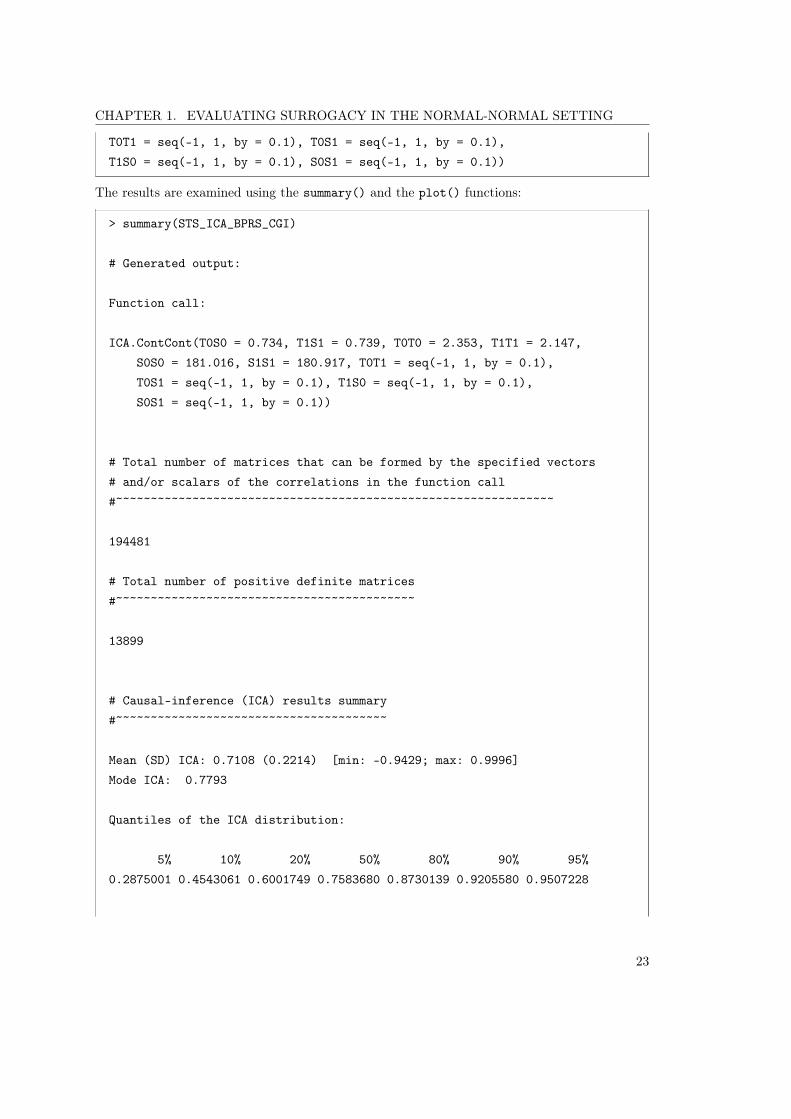
CHAPTER 1. EVALUATING SURROGACY IN THE NORMAL-NORMAL SETTING
T0T1 = seq(-1, 1, by = 0.1), T0S1 = seq(-1, 1, by = 0.1),T1S0 = seq(-1, 1, by = 0.1), S0S1 = seq(-1, 1, by = 0.1))
The results are examined using the summary() and the plot() functions:
> summary(STS_ICA_BPRS_CGI)
# Generated output:
Function call:
ICA.ContCont(T0S0 = 0.734, T1S1 = 0.739, T0T0 = 2.353, T1T1 = 2.147,S0S0 = 181.016, S1S1 = 180.917, T0T1 = seq(-1, 1, by = 0.1),T0S1 = seq(-1, 1, by = 0.1), T1S0 = seq(-1, 1, by = 0.1),S0S1 = seq(-1, 1, by = 0.1))
# Total number of matrices that can be formed by the specified vectors# and/or scalars of the correlations in the function call#~~~~~~~~~~~~~~~~~~~~~~~~~~~~~~~~~~~~~~~~~~~~~~~~~~~~~~~~~~~~~~~
194481
# Total number of positive definite matrices#~~~~~~~~~~~~~~~~~~~~~~~~~~~~~~~~~~~~~~~~~~~
13899
# Causal-inference (ICA) results summary#~~~~~~~~~~~~~~~~~~~~~~~~~~~~~~~~~~~~~~~
Mean (SD) ICA: 0.7108 (0.2214) [min: -0.9429; max: 0.9996]Mode ICA: 0.7793
Quantiles of the ICA distribution:
5% 10% 20% 50% 80% 90% 95%0.2875001 0.4543061 0.6001749 0.7583680 0.8730139 0.9205580 0.9507228
23

CHAPTER 1. EVALUATING SURROGACY IN THE NORMAL-NORMAL SETTING
> plot(STS_ICA_BPRS_CGI)
# Generated output:
ICA
ρ∆
Percentage
−1.0 −0.5 0.0 0.5 1.0
0.00
0.05
0.10
0.15
0.20
0.25
The output of the summary() function shows that a total of 194, 481 matrices can be formed, ofwhich 13, 899 were positive definite. Compared to the case where S = BPRS and T = PANSS,the mean value for the estimates of ⇢� is much lower now and the variability of the distribution islarger (M = 0.711, SD = 0.221, range [�0.943; 0.999]). Clearly, the results are highly sensitiveto the assumptions regarding the unidentifiable correlations. Consequently, the assessment ofthe appropriateness of �S = the individual causal treatment effect on the BPRS as a surrogatefor �T = the individual causal treatment effect on the CGI is largely a matter of unverifiableassumptions. Therefore, it may be concluded that the validity of the BPRS score as a surrogatefor the CGI score is not clearly established.
Causal diagrams To explore the typical assumptions regarding the unidentified correlationsthat are associated with a range of ⇢� values, the function CausalDiagramContCont() canagain be used. For example, the following codes provide causal diagrams that shows the mediancorrelations between the potential outcomes for ⇢� � 0.70 and ⇢� 0.70:
> CausalDiagramContCont(STS_ICA_BPRS_CGI, Min = 0.7, Max = 1)
# Generated output:
24
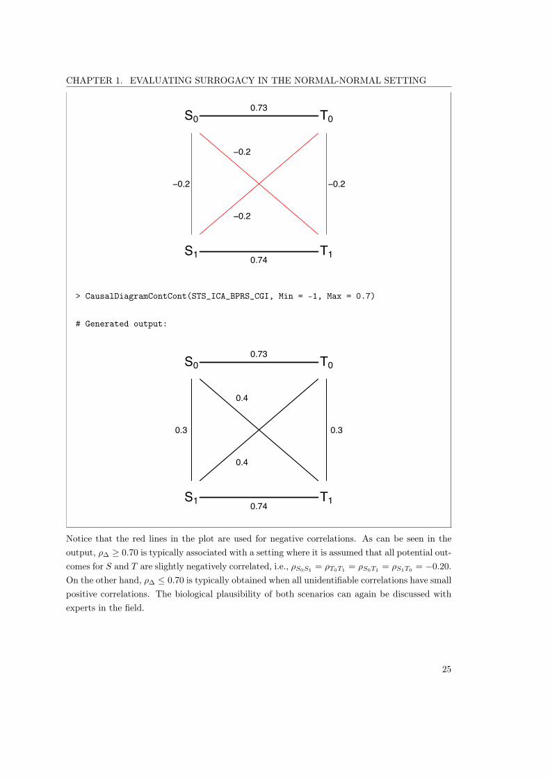
CHAPTER 1. EVALUATING SURROGACY IN THE NORMAL-NORMAL SETTING
S0
S1
−0.2
T0
T1
−0.2
−0.2
0.73
0.74
−0.2
> CausalDiagramContCont(STS_ICA_BPRS_CGI, Min = -1, Max = 0.7)
# Generated output:
S0
S1
0.3
T0
T1
0.4
0.4
0.73
0.74
0.3
Notice that the red lines in the plot are used for negative correlations. As can be seen in theoutput, ⇢� � 0.70 is typically associated with a setting where it is assumed that all potential out-comes for S and T are slightly negatively correlated, i.e., ⇢S0S1 = ⇢T0T1 = ⇢S0T1 = ⇢S1T0 = �0.20.On the other hand, ⇢� 0.70 is typically obtained when all unidentifiable correlations have smallpositive correlations. The biological plausibility of both scenarios can again be discussed withexperts in the field.
25

CHAPTER 1. EVALUATING SURROGACY IN THE NORMAL-NORMAL SETTING
1.3.3 The plausibility of finding a good surrogate
A lot of methodological work has been carried out to develop strategies to evaluate surrogatemarkers (for an overview, see Burzykowski, Molenberghs and Buyse, 2005), but the questionregarding the existence of a valid surrogate endpoint has been largely left unanswered. Indeed,given a clinically relevant true endpoint and a treatment of interest, one could wonder whetherthere exists a good surrogate marker in the first place.
As was detailed in Section 3.2.6 of Van der Elst (2016), the prediction mean squared error(PMSE) and ⇢2min can be used to assess the plausibility of finding a good surrogate given aparticular T . In the Surrogate package, the function ICA.ContCont() can be used to compute�, and MinSurrContCont() can be used to compute ⇢2min for a desired precision (a fixed valuefor �). This will be illustrated in the next sections using the data of the case study.
1.3.3.1 BPRS as a surrogate for PANSS
The function ICA.ContCont() can be used to compute the vector of values for � (PMSE). Usingthe fitted object STS_ICA_BPRS_PANSS (see Section 1.3.2.1), a plot that depicts the distributionof � across all plausible ‘realities’ can be obtained using the code:
> plot(STS_ICA_BPRS_PANSS, Good.Surr = TRUE, ICA = FALSE, breaks = 16)
# Generated output:
δ
Percentage
20 40 60 80
0.0
0.1
0.2
0.3
As can be seen, most � � 40. The 5
th percentile of the vector of � and its maximum value canbe obtained using the following code:
26

CHAPTER 1. EVALUATING SURROGACY IN THE NORMAL-NORMAL SETTING
> quantile(STS_ICA_BPRS_PANSS$GoodSurr$delta, c(0.05))
# Generated output:5%
37.1181
> max(STS_ICA_BPRS_PANSS$GoodSurr$delta)
# Generated output:[1] 83.939899
Thus 95% of the obtained � values lay between 37.118 and 83.940. This means that the individualcausal treatment effect on S allows for the prediction of the individual causal treatment effecton T with a PMSE that lies between about 6 and 9 points.
The function MinSurrContCont() can be used to compute ⇢2min for a fixed value of � (thedesired prediction precision) given the estimable variances b�T0T0 and b�T1T1 and a specified gridof values G for the unidentified parameter ⇢T0T1 . For example, the following code can be usedto obtain ⇢2min for � = 81 (corresponding with an average prediction error of 9 points), withb�T0T0 = 544.329 and b�T1T1 = 550.660 (see Section 1.3.2.1) and G = {�1, �0.90, ..., 1} for ⇢T0T1 :
> Rho2_min_BPRS_PANSS <- MinSurrContCont(T0T0 = 544.329, T1T1 = 550.66,Delta = 81, T0T1 = seq(-1, 1, by = 0.1))
A summary and histogram of the ⇢2min can be obtained using the codes:
> summary(Rho2_min_BPRS_PANSS)
# Generated output:
Function call:
MinSurrContCont(T0T0 = 544.329, T1T1 = 550.66, Delta = 81, T0T1 = seq(-1,1, by = 0.1))
# Rho2.Min results summary (Inf values are excluded)#~~~~~~~~~~~~~~~~~~~~~~~~~~~~~~~~~~~~~~~~~~~~~~~~~~~~~
27

CHAPTER 1. EVALUATING SURROGACY IN THE NORMAL-NORMAL SETTING
Mean (SD) Rho^2_min: 0.8669 (0.1653) [min: 0.2604; max: 0.9630]
Quantiles of the Rho2.Min distribution:
5% 10% 20% 50% 80% 90% 95%0.6116690 0.7411044 0.8446589 0.9293890 0.9543103 0.9591197 0.9611637
> plot(Rho2_min_BPRS_PANSS, main = (delta ~ "=81"))
# Generated output:
δ =81
ρmin2
Percentage
0.2 0.4 0.6 0.8 1.0
0.0
0.1
0.2
0.3
0.4
0.5
0.6
The output of the summary() function shows that the mean ⇢2min value was about 0.867, and⇢2min � 0.612 in 95% of the cases. Thus, a candidate S should produce a ⇢2� of about (at least)0.612 to achieve the desired average prediction error of 9 points in the prediction of the individualcausal treatment effects on T .
Obviously, the plausibility of finding a good surrogate is related to the desired prediction preci-sion. The previous analysis may help to find a reasonable balance between these two components.For example, suppose that we are willing to take more risk and use � = 225 (corresponding withan average prediction error of 15 points):
> Rho2_min_BPRS_PANSS_2 <- MinSurrContCont(T0T0 = 544.329,T1T1 = 550.66, Delta = 225, T0T1 = seq(-1, 1, by = 0.1))
The summary information and histogram of ⇢2min can be obtained using the commands:
28

CHAPTER 1. EVALUATING SURROGACY IN THE NORMAL-NORMAL SETTING
> summary(Rho2_min_BPRS_PANSS_2)
# Generated output:
Function call:
MinSurrContCont(T0T0 = 544.329, T1T1 = 550.66, Delta = 225, T0T1 = seq(-1,1, by = 0.1))
# Rho2.Min results summary (Inf values are excluded)#~~~~~~~~~~~~~~~~~~~~~~~~~~~~~~~~~~~~~~~~~~~~~~~~~~~~~
Mean (SD) Rho^2_min: 0.7191 (0.2377) [min: -0.0273; max: 0.8973]
Quantiles of the Rho2.Min distribution:
5% 10% 20% 50% 80% 90% 95%0.2808456 0.4520649 0.6301383 0.8131983 0.8745950 0.8870444 0.8923917
> plot(Rho2_min_BPRS_PANSS_2)
# Generated output:
29

CHAPTER 1. EVALUATING SURROGACY IN THE NORMAL-NORMAL SETTING
δ =225
ρmin2
Percentage
−0.2 0.0 0.2 0.4 0.6 0.8 1.0
0.0
0.1
0.2
0.3
0.4
0.5
The output now shows that the mean ⇢2min = 0.719, and ⇢2min � 0.281 in 95% of the settings.Thus a candidate S should produce a ⇢2� of about (at least) 0.281 to achieve the prediction ofthe individual causal treatment effects on T with an average prediction error of 15 points. Asexpected, this value is lower as compared to the value ⇢2min � 0.612 that was obtained when anaverage prediction error of 9 points was used.
1.3.3.2 BPRS as a surrogate for CGI
Using the fitted object STS_ICA_BPRS_CGI (see Section 1.3.2.2), a plot that depicts the distribu-tion of � across all plausible ‘realities’ can be obtained using the command:
> plot(STS_ICA_BPRS_CGI, Good.Surr = TRUE, ICA = FALSE, breaks = 9)
# Generated output:
30

CHAPTER 1. EVALUATING SURROGACY IN THE NORMAL-NORMAL SETTING
δ
Percentage
0 1 2 3 4
0.00
0.05
0.10
0.15
As can be seen, most � lay in the [0.5; 3.5] interval. Thus, the individual causal effect on theCGI can be predicted using the individual causal treatment effect on the BPRS with a predictionerror between about 0.7 and 1.9 points.
The function MinSurrContCont() can be used to compute ⇢2min for a fixed value of �. Forexample, the following code can be used to obtain ⇢2min for � = 1 (corresponding with an averageprediction error of 1 point on the 7-point CGI scale), with b�T0T0 = 2.353 and b�T1T1 = 2.147 (seeSection 1.3.2.2) and G = {�1, �0.90, ..., 1} for ⇢T0T1 :
> Rho2_min_BPRS_CGI <- MinSurrContCont(T0T0 = 2.353, T1T1 = 2.147,Delta = 1, T0T1 = seq(-1, 1, by = 0.1))
A summary and histogram of the ⇢2min can be obtained using the codes:
> summary(Rho2_min_BPRS_CGI)
# Generated output:Function call:
MinSurrContCont(T0T0 = 2.353, T1T1 = 2.147, Delta = 1, T0T1 = seq(-1,1, by = 0.1))
# Rho2.Min results summary (Inf values are excluded)#~~~~~~~~~~~~~~~~~~~~~~~~~~~~~~~~~~~~~~~~~~~~~~~~~~~~~
Mean (SD) Rho^2_min: 0.6966 (0.2561) [min: -0.1065; max: 0.8888]
31

CHAPTER 1. EVALUATING SURROGACY IN THE NORMAL-NORMAL SETTING
Quantiles of the Rho2.Min distribution:
5% 10% 20% 50% 80% 90% 95%0.2243130 0.4084667 0.6003414 0.7979605 0.8643237 0.8777851 0.8835676
> plot(Rho2_min_BPRS_CGI, main = (delta ~ "=1"))
# Generated output:
δ =1
ρmin2
Percentage
−0.2 0.0 0.2 0.4 0.6 0.8 1.0
0.0
0.1
0.2
0.3
0.4
The output shows that the mean ⇢2min value was 0.697, and ⇢2min � 0.224 in 95% of the cases.Thus, a candidate S should produce a ⇢2� of about (at least) 0.224 to achieve the desired levelof accuracy in the prediction of the individual causal treatment effects on T .
1.4 The multiple-trial setting
1.4.1 Expected causal association (ECA)
In the meta-analytic framework, two quantities are used to assess surrogacy. First, the individual-level surrogacy coefficient, which is defined as the treatment- and trial-corrected correlationbetween S and T . Second, the trial-level surrogacy coefficient, which is the correlation betweenthe expected causal treatment effects on S and T (ECA).
The function BifixedContCont() implements the two-stage bivariate fixed-effect modellingapproach (for details, see Tibaldi et al., 2003). The use of this function is illustrated in the next
32

CHAPTER 1. EVALUATING SURROGACY IN THE NORMAL-NORMAL SETTING
two sections.
1.4.1.1 BPRS as a surrogate for PANSS
The following code can be used to assess whether the BPRS is an appropriate surrogate forthe PANSS, based on expected causal effects using the reduced bivariate fixed-effect modellingapproach with treating psychiatrist (investigator) as the trial/clustering unit:
> MTS_ECA_BPRS_PANSS <- BifixedContCont(Dataset = Schizo, Surr = BPRS,True = PANSS, Treat = Treat, Pat.ID = Id, Trial.ID = InvestId,Model = "Reduced")
A summary of the results can be obtained with the following code:
> summary(MTS_ECA_BPRS_PANSS)
# Generated output:
Function call:
BifixedContCont(Dataset = Schizo, Surr = BPRS, True = PANSS,Treat = Treat, Trial.ID = InvestId, Pat.ID = Id, Model = "Reduced")
# Data summary and descriptives#~~~~~~~~~~~~~~~~~~~~~~~~~~~~~~~~~~~~~~~~~~~~~~~~~~~~~~~~~~~~~~~
Total number of trials: 150Total number of patients: 2020M(SD) patients per trial: 13.4667 (10.1165) [min: 2; max: 52]Total number of patients in experimental treatment group: 1497Total number of patients in control treatment group: 523
Mean surrogate and true endpoint values in each treatment group:
Control.Treatment Experimental.treatmentSurrogate -6.6577 -8.9873True endpoint -11.5277 -16.1222
33

CHAPTER 1. EVALUATING SURROGACY IN THE NORMAL-NORMAL SETTING
Var surrogate and true endpoint values in each treatment group:
Control.Treatment Experimental.treatmentSurrogate 182.8884 181.2518True endpoint 552.2727 549.4296
Correlations between the true and surrogate endpoints in thecontrol (r_T0S0)and the experimental treatment groups (r_T1S1):
Estimate Standard Error CI lower limit CI upper limitr_T0S0 0.9599 0.0062 0.9563 0.9632r_T1S1 0.9638 0.0059 0.9606 0.9668
# Meta-analytic results summary#~~~~~~~~~~~~~~~~~~~~~~~~~~~~~~~~~~~~~~~~~~~~~~~~~~~~~~~~~~~~~~~
R2 Trial Standard Error CI lower limit CI upper limit0.9199 0.0127 0.8951 0.9447
R2 Indiv Standard Error CI lower limit CI upper limit0.9276 0.0031 0.9215 0.9337
R Trial Standard Error CI lower limit CI upper limit0.9591 0.0233 0.9439 0.9702
R Indiv Standard Error CI lower limit CI upper limit0.9631 0.0060 0.9494 0.9732
The summary() function provides descriptive information such as the number of trials/clusters,the total number of patients, the mean number of patients per trial/cluster, and the means andvariances of S and T , as well as their correlations in both treatment groups. The surrogacyestimates bRtrial (ECA) and bRindiv are given at the end of the output.
As can be seen, the bRtrial estimate equalled 0.959 (CI95% = [0.944; 0.970]), indicating thatthere is a strong association between the expected causal treatment effects on S = BPRS and
34
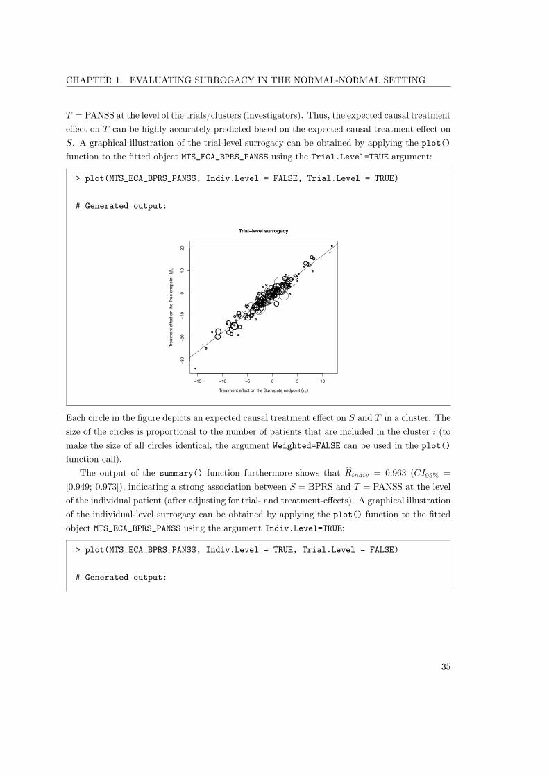
CHAPTER 1. EVALUATING SURROGACY IN THE NORMAL-NORMAL SETTING
T = PANSS at the level of the trials/clusters (investigators). Thus, the expected causal treatmenteffect on T can be highly accurately predicted based on the expected causal treatment effect onS. A graphical illustration of the trial-level surrogacy can be obtained by applying the plot()function to the fitted object MTS_ECA_BPRS_PANSS using the Trial.Level=TRUE argument:
> plot(MTS_ECA_BPRS_PANSS, Indiv.Level = FALSE, Trial.Level = TRUE)
# Generated output:
●
●
●
●
●●
●
●
●
●
●●
●
●
●
●
●
●
●
●
●
●
●
●
●
●
●
●
●
●
●
●
●●
●
●
●
●
●
●
●
●●
●
●
●
●●
●
●
●
●
●
●
●
●
●
●
●
●
●
●
●
●
●
●
●
●●
●
●
●
●●
●
●
●
●
●●
●
●
●
●
●
●
●
●
●
●
●
●
●
●
●
●●
●
●●
●
●●
●
●
●●
●
●
●
●●
●
●
●
●
●
●
●
●
●
●
●
●
●●
●
●
●
●
●
−15 −10 −5 0 5 10
−30
−20
−10
010
20
Trial−level surrogacy
Treatment effect on the Surrogate endpoint (αi)
Trea
tmen
t effe
ct o
n th
e Tr
ue e
ndpo
int (β
i)
Each circle in the figure depicts an expected causal treatment effect on S and T in a cluster. Thesize of the circles is proportional to the number of patients that are included in the cluster i (tomake the size of all circles identical, the argument Weighted=FALSE can be used in the plot()function call).
The output of the summary() function furthermore shows that bRindiv = 0.963 (CI95% =
[0.949; 0.973]), indicating a strong association between S = BPRS and T = PANSS at the levelof the individual patient (after adjusting for trial- and treatment-effects). A graphical illustrationof the individual-level surrogacy can be obtained by applying the plot() function to the fittedobject MTS_ECA_BPRS_PANSS using the argument Indiv.Level=TRUE:
> plot(MTS_ECA_BPRS_PANSS, Indiv.Level = TRUE, Trial.Level = FALSE)
# Generated output:
35

CHAPTER 1. EVALUATING SURROGACY IN THE NORMAL-NORMAL SETTING
●
●
●
●
●
●
●
●
●
●
●
●
●
●
●
●
●
●
●
●
●
●
●
●
●
●
●
●
●
●
●
●
●
●
●● ●
●
●●
●
●
●
●
●
●
●
●
●
●
●●
●
●
●
●
●
●
●
●
●
●
●
●
●
●
●
●
●
●
●
●
●
●
●
●
●●●
●
●● ●
●
●
●
●
●
●
●
●
●●
●
●●
●
●
●
●
●
●
●
●
●
●
●
●
●
●
●
●
●
●
●
●
●
●
●
●
●
●
●
●
●
●
●
●●
●
●
●
●●
●
●
●
●
●
●●
●
●
●
●
●
●
●
●
●
●
●
●
●
●
● ●
●
●
●
●
●
●
●
●
●
●
●
●●
●
●
●
●●
●
●
●●
●●●
●
●
●
●●
●
●
●
●
●
●●
●
●
●●●
●
●
●
●
●
●
●
●●
● ●
●
●
●
●
●
●
●
●
●
●●
●
●
●
●
●
●
●
●
●
●
●
●
●
●●
●
●
●
●
●
●
●
●●
●
●
●
●●●
●
●●
●●
●
●
●
●
●
●
●
●
●
●
●
●
●
●
●
●
●
●
●
●
●
●
●●
●
●●
●
●●
●
●
●
●
●
●
●●
●
●●
●
●
●
●●
●
●
●
●
●
●●
●
●
●
●
●
●
●
●
●
●●
●
●
●
●
●
●●
●
●
●
●
●
●
●
●
●
●
●
●
●
●
●
●
●
●
●●
●
●
●
●
● ●●
●
●
●●
●
●
●
●
●●
●
●●●
●
●
●
●
●●
●
●
●
●
●
●
●
●
●
●
●
●
●
●
●
●
●
●
●
●
●
●
●
●
●
●
●
●●
●
●
●
●
●●
●●
●
●
●
●
●
●
●
●
●
●
● ●
●
●
●
●
●
●
●
●●
●
●
●
●
●
●
●
●
●
●
●
●
●
●●
●●●
●
●●●
●
●
●
●
●
●
●
●
●●
●●
●
●●
●
●
●
●
●
●
●
●●●
●
●
●
●
●
●
●
●●
●
●●
●
●
●
●
●
●●
●
●
●
●●
●
●
●●
●
●
●
●
●
●
●●
● ●●●
●●
●
●●●
●
●
●
●
●
●
●
●
●
●
●
●●
●●●
●
●●
●
●
● ●
●
●
●
●
●
●
●
●
●
●●
●
●
●
●
●
●
●
●●
●
●
●
●
●
●
●●
●
●
●
●
●●
●
●
●●
●
●
●
●
●
●
●
●
●
●
●
●
●
●
●
●
●
●●
●
●
●●
●
●
●
●
●
●
●
●
●
●
●
●
●
●
●
●
●●
●
●●
●
●
●
●
●
●
●
●
●
●
●
●
●●
●
●
● ●
●
●
●
●
●
●●
●
●
●●
●
●
●
●
●
●
●
●
●
●
●
●
●●
●
●
●
●
●
●
●
●
●
●
●
●
●
●
●
●
●
●
●
●
●
●
●
●
●
●
●
●
●
●
●
●
●
●
●
●●
●●
●
●
●
●
●
●●
●
●
●
●
●
●
●
●
●
●
●
●●
●
●
●
●
●
●
●
●
●
●
●
●
●
●
●
●
●
●●●
●
●
●
●
●●
●
●
●
●
●
●●
●
●
●
●
●●
●
●
●
●
●
●
●
●
●
●
●
●
●
●
●
●
●
●●
●
●
●
●
●
●
●
●●
●
●
●●
●
●
●
●
●
●
●
●
●
●●
●
●
●
●
●
●
●
●
●
●
●
●
●
●●
●
●
●
●●
●
●
●
●
●
●
●
●
●●
●
●
●
●
●
●
●
●
●
●
●●
●●
●
●
●● ●
● ●
●
●
●
●
●
●
●
●
●
●
●
● ●
●●
●
●
●
●
●● ●
●
●
●
●
●
●
●
●
●
●●
●●
●●
●●
● ●
●
●
●●
●● ●
●
●
●
●●
●
●
●
●
●
●
●
●
●
●
●
●●
●
●
●
●
●
●●
●
●
●●
●
●
●●
●
●
●
●
●
●
●
●
●
●
●
●
●●
●
●
●●
●
●
●
●
●
●
●
●
●
●
●●
●
●
●
●
●
●
●
●
●
●
●●
●
●
●
●
●
●
● ●
●
●
●
●
●
●
●●
●
●●
●
●
●
●
●
●
●
●
●
●
●
●
●
●
●●
●
●
●●
●●
●
●
●
●●
●
●
●
●
●
●
●
●
●
●
●
●
●
●
●
●
●
●
●●
●
●
●●
●
●
●
●
●
●●●
●
●
●
●●
●
●
●
●
●
●●
●
●
●
●
●●
●
●
●●
●
●
●
●
●
●
●
●
●
●
●
●
●
●●
●
●
●
●
●
●
●
● ●
●
●
●●
●
●
●
●
●●
●●
●
●
●
●
●
●
●
●●●
●●
●
●
●
●
●
●
●
●
●
●
●
●
●
●
●
●
●●●
●
●
●
● ●
●
●
●
●●
●
●
●●
●
●●
●
●
●
●
●●●
●
●
●
●
●
●
●
●
●
●
●
●
●
●
●
●
●
●
●
●
●
●
●
●
●
●
●
●
●
●
●●
●
●
●
●
●
●
●
●
●
●
●
●●
●
●
●
●
●●
●
●
●
● ●
●
●
●
●
●
●
●
●
●●
●
●●
●
●
●
●●
●●●
●
●
●
●
●●●
●
●
●●
● ●●
●
●
●
●● ●
●●
●
●●
●
●
●
●●
●
●
●
●
●
●●●●
●
●
●
●●
●
●
●
●
●
●
●●
●
●
●
●
●
●
● ●
●●
●
●
●
●
●
●
● ●
●
●●●
●
●
●
● ●
●
●
●●
●
●
●
●
●
●
●
●
●
●
●●●
●
●
●
●
●
●
●
●
●
●
●
●
●
●●
●
●
●●●
●
●
●●
●
●
●●
●
● ●
●
●
●
●●
●
●●●●
●●
●
●●
●
●●
●
●
●●
●
●
●●
●
●
●
●
●
●
●
●●
●
●
●●
●
●
●
●
●
●
●●
●
●●
●
●
●●
●●
●
●
●
●
●
●
●
●
●●
●●●
●
●
●
● ● ●
●●
●
●
●
●
●
●
●
●
●
●
●
●
●●
●●
●
●
●
●
●
●
●
●
●
● ●
●
●
●
●●
●
●●
●
●
●
●
●
●
●
●●
●
●
●
●
●
●●●
●
●
●
●●
●●
●
●●
●
●
●
●
●
●
●
●
●
●
●
●
●
●●
●
●
●
●
●●
●●
●
●
●
●
●
● ●●
●
●
●●
●
●
●●
●●
●
●
● ●
●
●
●
●
●●
●
●●
●●
●
●
●●
●
●
●
●●
●
●
●●
●
●
●
●
●
●
●
●
●
●
●●
●
●
●
●
●
●
●
●
●●
●
●●
●
●
●●
●
●
●
●
●
●
●●
●
●●
●
●
●
●
●
●
●●
●
●
●
●
●
●
●
●●
●
●
●
●
●
●
●
●
●
● ●●
●
●
●
●
●
●
●
●
●
●
●
●
●
●
●
●
●
●
●
●●
●
●
●
●
●
●
●
●
●
●
●
●
●
●
●
●
●
●
●● ●
●
●●●●
●
●●
●
●
●
●
●
●
●
●
●
●
●
●
●
●
●
●
●
●
●
●
●
●
●
●
●●
●
●
●
●
●
●●
● ●
●
●
●
●
●
●
●●
●
●
●
●
●
●
●
●
●
●
●
●
●
●
●
●
●● ●
●
●
●
●
●
●
●
●
●
●
●
●
●
●
●
●
●
●
●
●
●
●
●
●
●
●●
●
●
●
●
●
●
●
●
●
●
●
●
●
●
●
●
●
●●
●●
●●
●●
●
●
●
●
●
●
●
●
●
●
●
●
●
●
●
●
●
●
●
●
●
●
●
●
●
●
●
●
●
●
●
●
●
●
●
●
●
●
●
●
●●
●
●
●
●●
●
●
●
●
●●
●●
●
●
●
●
●
●
●
●
●
●
●
●
●
●
●
●
●
●
●
●
●
●
●
●
●
●
●
●
●
●
●
●
●
●
●
●
●
●● ●●
●
●
●
●
●
●
●
●●
●●
●
●●
●
●
●
●●
●
●
●
●
●
●
●
●
●
●
●
●
●
●
●
●
●
●
●
●
●●
●
●
●●
●
●
●
●
●●
●
●
●
●
●
●
●
●
●
●
●
●
● ●
●
●●
●
●
●
●
●
●
●
●
●
●
●
● ●
●
●
●
●
●
●
●
●
●●●
●
●
●
●
●
●
●
●
−40 −20 0 20 40
−100
−50
050
100
Individual−level surrogacy
Residuals for the Surrogate endpoint (εSij)
Res
idua
ls fo
r the
Tru
e en
dpoi
nt (ε T
ij)
Overall, the analysis based on expected causal treatment effects in the MTS indicates that theBPRS score is an excellent surrogate for the PANSS score.
1.4.1.2 BPRS as a surrogate for CGI
The following code can be used to assess surrogacy based on expected causal effects (S = BPRS,T = CGI) in the MTS, using a weighted bivariate fixed-effect model with treating physician asthe clustering unit:
> MTS_ECA_BPRS_CGI <- BifixedContCont(Dataset = Schizo, Surr = BPRS,True = CGI, Treat = Treat, Pat.ID = Id, Trial.ID = InvestId,Model = "Reduced")
A summary of the results and a plot that depicts trial- and individual-level surrogacy can beobtained using the following code:
> summary(MTS_ECA_BPRS_CGI)
# Generated output:
Function call:
BifixedContCont(Dataset = Schizo, Surr = BPRS, True = CGI,Treat = Treat, Trial.ID = InvestId, Pat.ID = Id, Model = "Reduced")
# Data summary and descriptives
36

CHAPTER 1. EVALUATING SURROGACY IN THE NORMAL-NORMAL SETTING
#~~~~~~~~~~~~~~~~~~~~~~~~~~~~~~~~~~~~~~~~~~~~~~~~~~~~~~~~~~~~~~~
Total number of trials: 149Total number of patients: 2011M(SD) patients per trial: 13.4966 (10.0879) [min: 2; max: 52]Total number of patients in experimental treatment group: 1493Total number of patients in control treatment group: 518
Mean surrogate and true endpoint values in each treatment group:
Control.Treatment Experimental.treatmentSurrogate -6.6853 -8.9853True endpoint 3.4440 3.1936
Var surrogate and true endpoint values in each treatment group:
Control.Treatment Experimental.treatmentSurrogate 183.3727 181.0789True endpoint 2.3634 2.1589
Correlations between the true and surrogate endpoints in the control(r_T0S0) and the experimental treatment groups (r_T1S1):
Estimate Standard Error CI lower limit CI upper limitr_T0S0 0.7337 0.0152 0.7128 0.7532r_T1S1 0.7346 0.0151 0.7138 0.7541
# Meta-analytic results summary#~~~~~~~~~~~~~~~~~~~~~~~~~~~~~~~~~~~~~~~~~~~~~~~~~~~~~~~~~~~~~~~
R2 Trial Standard Error CI lower limit CI upper limit0.5159 0.0576 0.4031 0.6287
R2 Indiv Standard Error CI lower limit CI upper limit0.5412 0.0151 0.5117 0.5708
37

CHAPTER 1. EVALUATING SURROGACY IN THE NORMAL-NORMAL SETTING
R Trial Standard Error CI lower limit CI upper limit0.7183 0.0574 0.6302 0.7880
R Indiv Standard Error CI lower limit CI upper limit0.7357 0.0151 0.6520 0.8017
> plot(MTS_ECA_BPRS_CGI, Indiv.Level = FALSE, Trial.Level = TRUE)
# Generated output:
●
●
●
●
●●
●
●
●
●
●
●
●
●
●●
●
●
●●●
●
●
●
●●
●
●
●●
●
●
●
●
●
●●
●
●
●●
●●
●
●●
●
●●
●
●
●
●
●
●
●
●
●
●
●
●
●●
●
●
●
●
●
●
●
●● ●●
●●
●
●
●
●
●
●
●
●
●
●
●
●
●
●
●
●
●
●
●
●●
●
●
●
●●
●
●
●
●●
●
●
●
●
●
●
●
●
●
●
●
●
●
●
●
●
●
●
●
●
●
●
●
−15 −10 −5 0 5 10
−2.0
−1.5
−1.0
−0.5
0.0
0.5
1.0
1.5
Trial−level surrogacy
Treatment effect on the Surrogate endpoint (αi)
Trea
tmen
t effe
ct o
n th
e Tr
ue e
ndpo
int (β
i)
> plot(MTS_ECA_BPRS_CGI, Indiv.Level = TRUE, Trial.Level = FALSE)
# Generated output:
38

CHAPTER 1. EVALUATING SURROGACY IN THE NORMAL-NORMAL SETTING
●
●
●
●
●
●
●
●
●
●
●
●
●
●
●
●● ●
●
●●
●
●
●●
●
●
●
●
●
●
●
●●
●
●
●
●
●
●
●
● ●
●
●
●
●●
●
●
●
● ●
●
● ●
●
●
●
●
●
●
●●
● ●
●
●
●
●
●
●
●
●
●
●
●
●
●
●
●
●
●
●
●●
● ●
● ●
●●
●
●
●
●
●
●
●
●
● ●
●
●
●●
●●
●
●
●
●
●●
●
●
● ●
●
●●
●
●●
●
●
●
● ●
●
●
●●
●
●
●
●
●
●
●
●
●
●
●
●
●
●
●●● ●
●
●
●
●
●
● ●●
●
●
●
●
●
●
●
●
●
●
●
●
●
●●●
●
●
●●
●
●
●
●
●
●
●
●
●●
●● ●
●
●
●
●
●
●
●
●
● ●
●
●
●
●
●
●
●
●
●
●
●
●
●
● ●
●
●●
● ●
●
●
●
●
●●
●●
●
●
●
●
●●
●
●●
●
●
●
●
●
●
●
●●
● ●●
●
●
●
●
●
●
●
●
● ●●● ●
●
●
●
●
●
●
● ●
●
● ●
●
●
●
●
●
●
●
●
●
●
●
●
●
●
●
●
●
●
●
●
●
●
●
●
●
●
●
●
●
●
●
●
●
●
●
●
●
●
●
●
●
●
●
●
●
●
●
●
● ●●
●
●
●
●
●
●
●
●
●
●
●
●
●
●
●
●
● ●
●
●
●●
●
●
●
●
● ●
●
●
●
●
●
●
●
●
●
●●
●
●
● ●
●
●
●
●
●●
●●
●
●
●
●
●
●
●
●
●
●
●
●
●
● ●●
●
●
●
●
●
●
●
●
●
●●
●
●
●
●
●
●
●
●
●
●
●
●
●
●
●
●
●
●
●
● ●
●
●
●
●
●
●
●●●
●
●●
●
●
●
●
●
●
●
●●●
● ●
●
●
●
● ●
●●
●
● ●
●●
●●●
●
●
● ●●
●
●
●
●
●
●●
●
●
●
●
● ●●
●
● ●●●● ●
●
●
●
●●
●●
●
●●
●
● ●●
●
●
● ●
●
●●
●
●
●●●
●
●●
●
●●
● ●
●
●
●●
●
●
●
●
●
●
●
●
●
●
●●
●
●
●
●
●
●
●
●
●
●
●●●
●
●●
●
●●
●●
●
●● ●
●
●●●
●
●●●
●
●
●
●
●
●
●
●
●●
●
●
●
●
●
●
●
●
●
●●
●
●
●●
● ●
●
●
●
●
●
●●
●
●
●●
●
●
●
●
●
●
●
●
●
●●
●
●
●
●
●
●
●
●●
●
●
●
●
●
●
●●
●●
●
● ●
●
●
●●
●
●●●
● ●
●
●
●
●
●
●
●●
● ●●
●●
●
●
●
●
● ●
●
●
●
●
●
●
●
●
●
●
●
●
●
●
●
●
●
●
●
●
●
●
●
●
●
●
●
● ●
●
●
●
●
●
●
●
●
●
●
●
●
●
●●
●
●
● ●
●
●
●
●
●
●
●
●
●
●
●
●
●
●
●
● ●●
● ●
●
●
●
●
● ●●
● ●
●
●
●
●●
●
●
●
●
●
●
●
●
●
●
●
●
●●
●
●●
●
●
●●
●
●
●
●
●
●
●
●
●
●
●
●
●
●
●
●
●
●
●
●
●
●
●
●
●
●
●
●
●
●
●
●
●●●
●
●
●
●
●
●●
●●
●● ●
●
●●
●
●
●
●●
●
●
●
●
●
●●
●
●
●
● ● ●●
●
● ●
●
●
●
●●
●
●
●
●
●
●
●
●
●
●
●
●
●
●
●
●
●
●
●
●
● ●
●●
●
●
●
●
●
●
●
●●●
●
●
●
●
●
●
●
●
●●
●●
●
●
●
●
●
●
●
●
●
●
●
●
●
●
●
●
●
●
●●
●
●
●
●
●
●
●●
●
●
●
●
●
●
●●
●●
●
●
●●
●●
●
●
●
●●
●●
●
●●●
●●
●
●
●
●
●
●
●
●
●
●
●
●
●
● ●
●
●
● ●
●
●
●
●
●
●
●
●
●
●
●
●
●
●
●
●
●
●
●
●
●●
●
●
●
●●● ●
●
●
●
●
●
●
●
●
●
●
●
●
●
●
●
●●
●
●
●
●
●
●
●
●
●
●
●
●
●
●
●
●
●
●
●●
●
●
●
●
●●
●
●
●
●
●
●
●
●●
●
●
●
●
●●
●
●●
●
● ●●
●
●
●
●
●
●
●
●
●
●
●●
●
●●●
●
●
●
●
●
●
●
●
●
● ●
●
●
●
●● ●
●
●
●●
●
●
●
● ●
●
●
●
●
●
●
●
●
●
●
●
●
●
●
●
●
● ●
●
●
●●
●
●
●
●
●
●
●
●
●
●
●
●
●
●
●
●
●
●
● ●
●●
●
●●
●
● ●
●
●
●
●
●● ●
●
●
●
●
●
●
●
●
●
●
●●
●
●
●
●
●
●
●
●
●
●
●
●●●
●
●
●
●
●
●
●
●
●
●
●
●
●
●
●
●
●
●●
●
●
●
●● ●
●●
●
●
●
●
●
●
●
●
●
●●
●
●
●
●
●
●
● ●
●●
●
●
●
●
●●
●
●
●
●●●
●
● ●
●●●
●
●
●
●
●
●
●
●●
●
●
●
●
●
●● ●
●
●●
●
●
●
●
● ●
●
●●
●
●
●
●
●
●
●
●
●
●
●
●
●
●
● ●
●
●
●
●
●
●
●
●
●
●
●
●
●
● ●
●
●
●
●
●●●
●
●
●
●●
●
●
● ●●●
●
●
●
●●
●
●
●
●●
●
●
●
●●
●
●
●●
●
●●
●
●
●
●
●
●
●●
●
●●
●
●
● ●
●
● ●
●
●
●
●
●
●●
●
●●●●
●●
●
●●
●
●●
● ●
●
● ●
●
●
●
●
●●
●
●
●
●
●
●
●
●
●
●
●
●
●
●
●
●
●
● ●
●●
●
●
●
●
● ●
●
●
●
●
●
●
●
●
●
●
●
●●
●
●
●
●
● ●
●
●
● ●
● ●
●
●
●
●●
●
● ●
●●
●
●
●
●●
●
●●
●
●
●●
●
●●
●
●●
●
●
●
●
●
●
●●
●
●
● ●
●
●●
●
●
●
●
●
●
●
●
●
●
●
●
●
●
●
●
●
●
●
●●
●
● ●
●●●● ● ●
●
●
●
●
●
●
●
●
●
●
●
●●
●
●
●
●
●
●
●
●
● ● ●
●
● ●●
● ●
●
●
● ●
●
●● ●●
●
●
●
●
●
●
●
●
●
●●●
●
●●
●
●
●
● ●●
●
●
●
●
● ●
●
●
●
●●
●
●
●
● ●
●
●
●●
●
●
●
●
●
●
●
● ●●
●
●
●
● ●
●
●
●
●
●
●
● ●●
●
●
●
●
●
●
●
●
●
●
●
●
●
●
●
●
●
●
●
●
●
●
●●
●
●●
●
●
●
●
●
●
●
●
●
●
●
●
●
●
●
●
●
●
● ●
●●
●
● ●
●
●●
●
● ●●
●
●
●
●
● ●●
●
●
●
●
●
●
●
●
●
●
●
●
●
●
●
●
●
●
●●
●
●
●
●
●
●
●
●●
●
●
●
●
●
●
●
●
● ●
●
●
●
●
● ●
●
●
●
●
●
●
●
●
●
●
●
●●
●
●● ●● ●
●●
●
●
●
●
●
●
●
●
● ●
●●
●
● ●
●
●
●
●●
●
●
●
●
●
●
●
●
●
●
●
●
●
●
●
●●●●
●
●
●●
●●
●
●●
●
●
●
●
●
●
●
●
●
●
●●●
●
●
●
●
●
●
●
●●
●
●
●
●
●
●
●
●
●
●
●
● ●
●
●
●
●
●
●
●
●
●●
● ●
●
●
●
●
●
●
●
●
●
●
●
●●
●
●
●
●
● ●●
●
●●
●●
●
●
●
●
● ●
●
●
●
●
●
●
●
●
●
●
●●
●
●●
●
●
●
●
●
●
●
●
●
●
●
●
●
●
●
●
●
●
●
●●
●
●
● ●●
●
●
●
●
●
●
●
●
●
●
●
●
●
●
●
●
●
●
●
●
●
●
●
●●
●
●●●
●
●
●
●
●
●
●
●●●
●
●
●
●
●
●
●
●
●●
●
●
●
●
●
●
●
●
●
●
●
●●
●●
●
●
● ●
●
●
●
●
● ●
−40 −20 0 20 40
−20
24
Individual−level surrogacy
Residuals for the Surrogate endpoint (εSij)
Res
idua
ls fo
r the
Tru
e en
dpoi
nt (ε T
ij)
The output shows that bRtrial = 0.718 (CI95% [0.630; 0.788]), indicating that the accuracy bywhich the expected causal treatment effect on the T = CGI can be predicted based on theexpected causal treatment effect on S = BPRS is relatively low. Likewise, bRindiv = 0.736
(CI95% [0.652; 0.802]), indicating that the accuracy by which a patient’s T can be predicted asbased on S (after adjusting for cluster- and treatment-effects) is relatively low.
1.4.2 Meta-analytic individual causal association (MICA)
The Meta-Analytic Individual Causal Association (MICA; ⇢M ) is defined as the correlationbetween the individual causal treatment effects on S and T (for details, see Chapter 3 in Vander Elst, 2016):
⇢M =
pdbbdaaRtrial +
q��T0T0 + �T1T1 � 2
p�T0T0�T1T1⇢T0T1
� ��S0S0 + �S1S1 � 2
p�S0S0�S1S1⇢S0S1
�⇢�
q⇥dbb + �T0T0 + �T1T1 � 2
p�T0T0�T1T1⇢T0T1
⇤ ⇥daa + �S0S0 + �S1S1 � 2
p�S0S0�S1S1⇢S0S1
⇤ ,
(1.2)where daa and dbb are the variances of the expected causal treatment effects on S and T , Rtrial
is the correlation between the expected causal treatment effects on S and T (ECA), ⇢XY isthe correlation between X and Y , �XX is the variance of X, and ⇢� is the individual causalassociation (see Section 1.3.2).
As was also the case with the ICA, MICA is a conceptually appealing measure of surrogacybut its practical use is challenging because the correlations between the counterfactuals (i.e.,⇢S0T1 , ⇢S1T0 , ⇢T0T1 and ⇢S0S1) are not estimable from the data. To deal with this issue, thesimulation-based approach detailed in Van der Elst (2016) was implemented in the functionMICA.ContCont().
In the function call, the user specifies the estimable quantities ( bRtrial, bdaa, bdbb, b⇢S0T0 , b⇢S1T1 ,b�S0S0 , b�S1S1 , b�T0T0 and b�T1T1) and the scalars or vectors that should be considered for the
39

CHAPTER 1. EVALUATING SURROGACY IN THE NORMAL-NORMAL SETTING
unidentifiable parameters (⇢S0T1 , ⇢S1T0 , ⇢T0T1 and ⇢S0S1). The use of this function will beillustrated below for the cases where S = BPRS and T = PANSS, and S = BPRS and T = CGI.
1.4.2.1 BPRS as a surrogate for PANSS
The estimates for Rtrial, ⇢S0T0 , ⇢S1T1 , �S0S0 , �S1S1 , �T0T0 , and �T1T1 can be obtained by applyingthe summary() function to the fitted object MTS_ECA_BPRS_PANSS (see Section 1.4.1.1). Theestimated variances of the expected causal treatment effects on S and T (daa and dbb) can beobtained using the following code:
> MTS_ECA_BPRS_PANSS$D.Equiv
# Generated output:
Treatment.S Treatment.TTreatment.S 22.62958 38.75356Treatment.T 38.75356 71.28230
Using the obtained estimates and the grid of values G = {�1, �0.90, ..., 1} for the unidentifiedcorrelations, the ⇢M values can be obtained using the following code:
> MTS_MICA_BPRS_PANSS <- MICA.ContCont(Trial.R = 0.959, D.aa = 22.630,D.bb = 71.282, T0S0 = 0.96, T1S1 = 0.964, S0S0 = 182.888,S1S1 = 181.252, T0T0 = 552.273, T1T1 = 549.43,T0T1 = seq(-1, 1, by = 0.1), T0S1 = seq(-1, 1, by = 0.1),T1S0 = seq(-1, 1, by = 0.1), S0S1 = seq(-1, 1, by = 0.1))
A summary of the obtained ⇢M values can be obtained using the following commands:
> summary(MTS_MICA_BPRS_PANSS)
# Generated output:Function call:
MICA.ContCont(Trial.R = 0.959, D.aa = 22.63, D.bb = 71.282,T0S0 = 0.96, T1S1 = 0.964, T0T0 = 552.273, T1T1 = 549.43,S0S0 = 182.888, S1S1 = 181.252, T0T1 = seq(-1, 1, by = 0.1),T0S1 = seq(-1, 1, by = 0.1), T1S0 = seq(-1, 1, by = 0.1),S0S1 = seq(-1, 1, by = 0.1))
40

CHAPTER 1. EVALUATING SURROGACY IN THE NORMAL-NORMAL SETTING
# Total number of matrices that can be formed by the specified vectors# and/or scalars of the correlations in the function call#~~~~~~~~~~~~~~~~~~~~~~~~~~~~~~~~~~~~~~~~~~~~~~~~~~~~~~~~~~~~~~~
194481
# Total number of positive definite matrices#~~~~~~~~~~~~~~~~~~~~~~~~~~~~~~~~~~~~~~~~~~~
343
# Causal-inference (MICA) results summary#~~~~~~~~~~~~~~~~~~~~~~~~~~~~~~~~~~~~~~~
Mean (SD) MICA: 0.9577 (0.0285) [min: 0.7515; max: 0.9852]Mode MICA: 0.9731
Quantiles of the MICA distribution:
5% 10% 20% 50% 80% 90% 95%0.9086699 0.9277713 0.9456289 0.9668705 0.9755264 0.9780773 0.9793051
The output shows that a total of 194, 481 matrices can be formed based on the estimable cor-relations b⇢S0T0 and b⇢S1T1 and all possible combinations of the values in G for the unidentifiablecorrelations. Of these matrices, only 343 were positive definite. The mean of the ⇢M = 0.958,and 95% of the ⇢M values exceeded 0.909. The variability of ⇢M was small (SD = 0.029, range[0.752; 0.985]), indicating that the sensitivity of the results with respect to the assumptionsregarding the unidentifiable correlations was relatively small. Overall, the analyses based onindividual causal effects in the MTS indicate that the BPRS is an appropriate surrogate for thePANSS (in line with the results based on expected causal effects).
Notice that, in line with expectations, the SD and range of ⇢M is smaller than the SD andrange of ⇢� (see Section 1.3.2.1), because the trial-level information is taken into account in thecomputation of ⇢M .
A histogram of the distribution of ⇢M can be obtained by applying the plot() command tothe fitted object MTS_MICA_BPRS_PANSS (of class MICA.ContCont()):
> plot(MTS_MICA_BPRS_PANSS, MICA = TRUE, ICA = FALSE)
# Generated output:
41

CHAPTER 1. EVALUATING SURROGACY IN THE NORMAL-NORMAL SETTING
MICA
ρM
Percentage
0.75 0.80 0.85 0.90 0.95 1.00
0.0
0.1
0.2
0.3
0.4
0.5
0.6
Causal diagrams The function CausalDiagramContCont() provides a causal diagram thatshows the median correlations between the potential outcomes for a specified range of values for⇢M (similarly as was the case for ⇢�, see above). For example, the following codes provides suchdiagrams for ⇢M � 0.90 and ⇢M 0.90:
> CausalDiagramContCont(MTS_MICA_BPRS_PANSS, Min = 0.9, Max = 1)
# Generated output:
S0
S1
0
T0
T1
0
0
0.96
0.96
0
> CausalDiagramContCont(MTS_MICA_BPRS_PANSS, Min = -1, Max = 0.9)
42

CHAPTER 1. EVALUATING SURROGACY IN THE NORMAL-NORMAL SETTING
# Generated output:
S0
S1
0.8
T0
T1
0.8
0.8
0.96
0.96
0.8
As can be seen, the results are identical to those that were obtained for ⇢� (described in Section1.3.2.1).
1.4.2.2 BPRS as a surrogate for CGI
The estimates for Rtrial, ⇢S0T0 , ⇢S1T1 , and the variances of S and T that are needed as input forthe MICA.ContCont were provided earlier (see Section 1.4.1.2). Further, estimates of daa and dbb
are needed as input of the function. These can be obtained using the code:
> MTS_ECA_BPRS_CGI$D.Equiv # to obtain estimates for d_aa and d_bb
# Generated output:
Treatment.S Treatment.TTreatment.S 22.716329 2.0788811Treatment.T 2.078881 0.3212402
Using the obtained estimates and the grid of values G = {�1, �0.90, ..., 1} for the correla-tions between the potential outcomes, the ⇢M estimates can be obtained using the followingcommand:
> MTS_MICA_BPRS_CGI <- MICA.ContCont(Trial.R = 0.718, D.aa = 22.716,D.bb = 0.321, T0S0 = 0.734, T1S1 = 0.735, S0S0 = 183.373,S1S1 = 181.079, T0T0 = 2.363, T1T1 = 2.159,T0T1 = seq(-1, 1, by = 0.1), T0S1 = seq(-1, 1, by = 0.1),
43

CHAPTER 1. EVALUATING SURROGACY IN THE NORMAL-NORMAL SETTING
T1S0 = seq(-1, 1, by = 0.1), S0S1 = seq(-1, 1, by = 0.1))
A summary and histogram of the obtained ⇢M estimates can be obtained using the followingcommands:
> summary(MTS_MICA_BPRS_CGI)
# Generated output:
Function call:
MICA.ContCont(Trial.R = 0.718, D.aa = 22.716, D.bb = 0.321,T0S0 = 0.734, T1S1 = 0.735, T0T0 = 2.363, T1T1 = 2.159,S0S0 = 183.373, S1S1 = 181.079, T0T1 = seq(-1, 1, by = 0.1),T0S1 = seq(-1, 1, by = 0.1), T1S0 = seq(-1, 1, by = 0.1),S0S1 = seq(-1, 1, by = 0.1))
# Total number of matrices that can be formed by the specified vectors# and/or scalars of the correlations in the function call#~~~~~~~~~~~~~~~~~~~~~~~~~~~~~~~~~~~~~~~~~~~~~~~~~~~~~~~~~~~~~~~
194481
# Total number of positive definite matrices#~~~~~~~~~~~~~~~~~~~~~~~~~~~~~~~~~~~~~~~~~~~
14099
# Causal-inference (MICA) results summary#~~~~~~~~~~~~~~~~~~~~~~~~~~~~~~~~~~~~~~~
Mean (SD) MICA: 0.7128 (0.1898) [min: -0.4787; max: 0.9839]Mode MICA: 0.7736
Quantiles of the MICA distribution:
5% 10% 20% 50% 80% 90% 95%0.3403669 0.4765764 0.6055082 0.7517271 0.8584296 0.9027517 0.9314159
44

CHAPTER 1. EVALUATING SURROGACY IN THE NORMAL-NORMAL SETTING
> plot(MTS_MICA_BPRS_CGI)
# Generated output:
MICA
ρM
Percentage
−0.5 0.0 0.5 1.0
0.00
0.05
0.10
0.15
0.20
0.25
The output shows that the mean ⇢M was moderate (⇢M = 0.713) and the variability was large(SD = 0.190, range [�0.479; 0.984]). These results indicate that the impact of the assumptionsregarding the unidentified correlations on ⇢M was large. Thus, in some scenario’s there is astrong association between the individual causal effects on S and T , whilst in other scenarios theassociation is very weak. Notice again that the SD and range of ⇢M is smaller than the SD andrange of ⇢� (see Section 1.3.2.2), because the trial-level information is taken into account in thecomputation of ⇢M .
Causal diagrams To explore the typical assumptions regarding the unidentified correlationsthat are associated with a range of ⇢M values, the function CausalDiagramContCont() can againbe used. For example, the following codes provide causal diagrams with the median correlationsbetween the counterfactuals for ⇢M � 0.70 and ⇢M 0.70:
> CausalDiagramContCont(MTS_MICA_BPRS_CGI, Min = 0.70, Max = 1)
# Generated output:
45
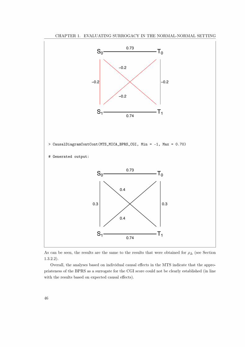
CHAPTER 1. EVALUATING SURROGACY IN THE NORMAL-NORMAL SETTING
S0
S1
−0.2
T0
T1
−0.2
−0.2
0.73
0.74
−0.2
> CausalDiagramContCont(MTS_MICA_BPRS_CGI, Min = -1, Max = 0.70)
# Generated output:
S0
S1
0.3
T0
T1
0.4
0.4
0.73
0.74
0.3
As can be seen, the results are the same to the results that were obtained for ⇢� (see Section1.3.2.2).
Overall, the analyses based on individual causal effects in the MTS indicate that the appro-priateness of the BPRS as a surrogate for the CGI score could not be clearly established (in linewith the results based on expected causal effects).
46

CHAPTER 1. EVALUATING SURROGACY IN THE NORMAL-NORMAL SETTING
1.5 Accounting for the sampling variability in the estima-
tion of ⇢S0T0 and ⇢S1T1
In the results that were detailed above, the sampling variability in the estimation of ⇢S0T0 and⇢S1T1 was not accounted for, e.g., in the analyses where S = BPRS and T = PANSS thesequantities were fixed as b⇢S0T0 = 0.960 and b⇢S1T1 = 0.964. To take the sampling variabilityin the estimation of ⇢S0T0 and ⇢S1T1 into account, ⇢S0T0 and ⇢S1T1 can be sampled from auniform distribution with (min, max) values equal to the upper and lower boundaries of the95% CIs of these correlations. The following command can be used to conduct such an analysisfor S = BPRS and T = PANSS in the single-trial setting, where CI95% = [0.956; 0.963] andCI95% = [0.961; 0.967] (and similarly for the other analyses):
> STS_ICA_BPRS_PANSS <- ICA.ContCont(T0S0 = runif(n = 200000, min = 0.956, max = 0.963),T1S1 = runif(n = 200000, min = 0.961, max = 0.967),S0S0 = 180.683, S1S1 = 180.943, T0T0 = 544.329, T1T1 = 550.66,T0T1 = seq(-1, 1, by = 0.1), T0S1 = seq(-1, 1, by = 0.1),T1S0 = seq(-1, 1, by = 0.1), S0S1 = seq(-1, 1, by = 0.1))
The results can be examined by using the summary() function:
> summary(STS_ICA_BPRS_PANSS)
# Generated output:Function call:
ICA.ContCont(T0S0 = runif(n = 2e+05, min = 0.956, max = 0.963),T1S1 = runif(n = 2e+05, min = 0.961, max = 0.967), T0T0 = 544.329,T1T1 = 550.66, S0S0 = 180.683, S1S1 = 180.943, T0T1 = seq(-1,
1, by = 0.1), T0S1 = seq(-1, 1, by = 0.1), T1S0 = seq(-1,1, by = 0.1), S0S1 = seq(-1, 1, by = 0.1))
# Total number of matrices that can be formed by the specified vectors# and/or scalars of the correlations in the function call#~~~~~~~~~~~~~~~~~~~~~~~~~~~~~~~~~~~~~~~~~~~~~~~~~~~~~~~~~~~~~~~
194481
47

CHAPTER 1. EVALUATING SURROGACY IN THE NORMAL-NORMAL SETTING
# Total number of positive definite matrices#~~~~~~~~~~~~~~~~~~~~~~~~~~~~~~~~~~~~~~~~~~~
346
# Causal-inference (ICA) results summary#~~~~~~~~~~~~~~~~~~~~~~~~~~~~~~~~~~~~~~~
Mean (SD) ICA: 0.9560 (0.0375) [min: 0.6021; max: 0.9930]Mode ICA: 0.9736
Quantiles of the ICA distribution:
5% 10% 20% 50% 80% 90% 95%0.8977303 0.9261374 0.9448691 0.9678203 0.9761053 0.9787146 0.9803783
As shown in the output, the ⇢� mean = 0.956, SD = 0.038, and range [0.602; 0.993], whereas the⇢� mean = 0.957, SD = 0.037, and range [0.620; 0.994] when the uncertainty in the estimationof ⇢S0T0 and ⇢S1T1 was not accounted for (see Section 1.3.2.1). The impact of accounting formeasurement error on the results was thus small. Similar results were obtained when samplinguncertainty was taken into account in the analysis of S = BPRS and T = CGI (data not shown).
48

Chapter 2
Evaluating surrogacy in the binary-
binary setting: case study analysis
details
2.1 Introduction
In this chapter, the use of the R package Surrogate for the analysis of the case study discussedin Chapter 4 of Van der Elst (2016) is detailed. In Section 2.2, the data are briefly described. InSection 2.3, the R2
H and SPF results are discussed for the analysis where S = clinically relevantchange on the BPRS and T = clinically relevant change on the PANSS. Section 2.4 focuses onthe analysis where S = clinically relevant change on the BPRS and T = clinically relevant changeon the CGI.
2.2 The dataset: a clinical trial in schizophrenia
In Section 2.1.1 of Van der Elst (2016), five clinical trials in schizophrenia were described. Here,a subset of this dataset is considered, i.e., the data of one of these clinical trial were used in theanalysis (recall that R2
H and SPF are metrics that were developed in the single-trial setting). Inthis trial, a total of 454 patients were treated for eight weeks. The endpoints of interest were thepresence or absence of clinically relevant changes in schizophrenic symptomatology as evaluatedby the BPRS/PANSS/CGI scales (see Section 2.1.1 of Van der Elst, 2016).
In the analyses below, it will be examined whether clinically meaningful change on the BPRS(a simpler and easier to administer scale to assess schizophrenic symptoms) is an appropriatesurrogate for clinically meaningful change on the PANSS (a more complex scale that requires
49

CHAPTER 2. EVALUATING SURROGACY IN THE BINARY-BINARY SETTING
more time and more skilled personnel for its administration). R code is also provided for theanalysis where it is examined whether clinically meaningful change on the BPRS is an appropriatesurrogate for clinically meaningful change on the CGI. To simplify the exposition, in the followingsections the names BPRS/PANSS/CGI will be used to refer to clinically meaningful change inthese scales.
The dataset (Schizo_Bin) is included in the Surrogate package. After installation of thepackage in R, the following code can be used to load the package and the schizophrenia datasetin memory for the subsequent analyses:
> library(Surrogate) # load the Surrogate library> data(Schizo_Bin) # load the data> head(Schizo_Bin) # have a look at the first observations
# Generated output:
Id InvestId BPRS_Bin PANSS_Bin CGI_Bin Treat1 1 1 1 1 0 12 2 2 1 1 0 13 3 2 0 0 1 -14 4 2 0 0 1 15 5 2 1 1 0 -16 6 3 1 1 0 1
The dataset contains six variables:
• ‘Id’: the identification number of the patient.
• ‘InvestId’: the identification number of the treating physician (investigator).
• ‘BPRS_Bin’: a binary endpoint coded as 1 = clinically meaningful change on the BPRSscale occurred, and 0 = otherwise.
• ‘PANSS_Bin’: a binary endpoint coded as 1 = clinically meaningful change on the PANSSscale occurred, and 0 = otherwise.
• ‘CGI_Bin’: a binary endpoint coded as 1 = clinically meaningful change on the CGI scaleoccurred, and 0 = otherwise.
• ‘Treat’: the treatment indicator, coded as �1 = control treatment (a dose of 10 mg. ofhaloperidol) and 1 = experimental treatment (a dose of 8 mg. of risperidone).
50

CHAPTER 2. EVALUATING SURROGACY IN THE BINARY-BINARY SETTING
2.3 BPRS as a surrogate for PANSS
2.3.1 Exploratory data analysis
The function MarginalProbs() can be used to obtain some descriptive summary measures ofthe data:
> MarginalProbs(Dataset = Schizo_Bin, Surr = BPRS_Bin,True = PANSS_Bin, Treat = Treat)
# Generated output:
$Theta_T0S0[1] 68.54167
$Theta_T1S1[1] 141.6104
$Freq.Cont
0 10 105 121 12 94
$Freq.Exp
0 10 94 71 11 116
$pi1_1_[1] 0.4215247
$pi0_1_[1] 0.05381166
$pi1_0_[1] 0.05381166
51
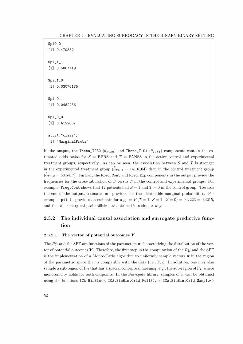
CHAPTER 2. EVALUATING SURROGACY IN THE BINARY-BINARY SETTING
$pi0_0_[1] 0.470852
$pi_1_1[1] 0.5087719
$pi_1_0[1] 0.03070175
$pi_0_1[1] 0.04824561
$pi_0_0[1] 0.4122807
attr(,"class")[1] "MarginalProbs"
In the output, the Theta_T0S0 (✓T0S0) and Theta_T1S1 (✓T1S1) components contain the es-timated odds ratios for S = BPRS and T = PANSS in the active control and experimentaltreatment groups, respectively. As can be seen, the association between S and T is strongerin the experimental treatment group (b✓T1S1 = 141.6104) than in the control treatment group(b✓T0S0 = 68.5417). Further, the Freq.Cont and Freq.Exp components in the output provide thefrequencies for the cross-tabulation of S versus T in the control and experimental groups. Forexample, Freq.Cont shows that 12 patients had S = 1 and T = 0 in the control group. Towardsthe end of the output, estimates are provided for the identifiable marginal probabilities. Forexample, pi1_1_ provides an estimate for ⇡1·1· = P (T = 1, S = 1 | Z = 0) = 94/223 = 0.4215,and the other marginal probabilities are obtained in a similar way.
2.3.2 The individual causal association and surrogate predictive func-
tion
2.3.2.1 The vector of potential outcomes Y
The R2H and the SPF are functions of the parameters ⇡ characterizing the distribution of the vec-
tor of potential outcomes Y . Therefore, the first step in the computation of the R2H and the SPF
is the implementation of a Monte-Carlo algorithm to uniformly sample vectors ⇡ in the regionof the parametric space that is compatible with the data (i.e., �D). In addition, one may alsosample a sub-region of �D that has a special conceptual meaning, e.g., the sub-region of �D wheremonotonicity holds for both endpoints. In the Surrogate library, samples of ⇡ can be obtainedusing the functions ICA.BinBin(), ICA.BinBin.Grid.Full(), or ICA.BinBin.Grid.Sample()
52

CHAPTER 2. EVALUATING SURROGACY IN THE BINARY-BINARY SETTING
(for details, see the Surrogate manual). Due to its better numerical performance, the functionICA.BinBin.Grid.Sample() is used here. The ICA.BinBin.Grid.Sample() function requiresthe user to specify the following main arguments:
• pi1_1_=, pi0_1_=, ..., pi_0_1=: the identifiable marginal probabilities that can be obtainedusing the MarginalProbs() function as shown earlier.
• Monotonicity=: the assumption that is made regarding monotonicity (for details, see theSurrogate package). In the current analysis, it is assumed that monotonicity (a strong andoften unverifiable assumption) does not hold. Such an analysis can be requested by usingthe Monotonicity=c("No") argument in the function call (the impact of monotonicity onthe results is examined in Section 2.3.3).
• M=: the number of runs that are conducted.
The following command can be used to request an analysis using M = 10, 000:
> ICA <- ICA.BinBin.Grid.Sample(pi1_1_=0.4215, pi0_1_=0.0538,pi1_0_=0.0538, pi_1_1=0.5088, pi_1_0=0.0307, pi_0_1=0.0482, Seed=1,Monotonicity=c("No"), M=10000) # Seed is used for reproducibility
The fitted object ICA contains the ⇡ vectors that are needed to compute R2H and SPF. These
vectors can be obtained using the command ICA$Pi.Vectors. For example, the following codegives the first ⇡ vector:
> ICA$Pi.Vectors[1:1,1:16]
# Generated output:
Pi_0000 Pi_0100 Pi_0010 Pi_0001 Pi_0101 Pi_10001 0.2834182 0.00165064 0.004011403 0.01415234 0.1716788 0.005595477
Pi_1010 Pi_1001 Pi_1110 Pi_1101 Pi_1011 Pi_11111 0.1192749 0.007882472 0.01047195 0.02701474 0.01546092 0.2762922
Pi_0110 Pi_0011 Pi_0111 Pi_11001 0.005270105 0.01070427 0.03381422 0.01330731
2.3.2.2 The individual causal association (R2H)
The computation of R2H using the Surrogate package is straightforward, as the aforementioned
ICA.BinBin.Grid.Sample() function (see Section 2.3.2.1) also computes this metric.
The summary() function can be applied to the fitted ICA object to obtain descriptive statisticsfor these metrics:
53

CHAPTER 2. EVALUATING SURROGACY IN THE BINARY-BINARY SETTING
> summary(ICA)
# Generated output (restricted):
Function call:
ICA.BinBin.Grid.Sample(pi1_1_ = 0.4215,pi1_0_ = 0.0538, pi_1_1 = 0.5088, pi_1_0 = 0.0307, pi0_1_ = 0.0538,pi_0_1 = 0.0482, Monotonicity = c("No"), M = 10000, Seed = 1)
# Total number of valid Pi vectors#~~~~~~~~~~~~~~~~~~~~~~~~~~~~~~~~~
86
# R2_H results summary#~~~~~~~~~~~~~~~~~~~~~~~~~~~~~~~~~
Mean (SD) R2_H: 0.5280 (0.0963) [min: 0.2352; max: 0.6951]Mode R2_H: 0.5654
Quantiles of the R2_H distribution:
5% 10% 20% 50% 80% 90% 95%0.3319 0.3910 0.4828 0.5475 0.5912 0.6291 0.6412
# R_H results summary#~~~~~~~~~~~~~~~~~~~~~~~~~~~~~~~~~
Mean (SD) R_H: 0.7231 (0.0720) [min: 0.4850; max: 0.8337]Mode R_H: 0.7519
Quantiles of the R_H distribution:
5% 10% 20% 50% 80% 90% 95%
54

CHAPTER 2. EVALUATING SURROGACY IN THE BINARY-BINARY SETTING
0.5761 0.6253 0.6948 0.7399 0.7689 0.7932 0.8007
# Theta_T results summary#~~~~~~~~~~~~~~~~~~~~~~~~~~~~~~~~~
Mean (SD) Theta_T: 5.6613 (12.0080) [min: 0.0278; max: 86.5034]Mode Theta_T: 0.6469
Quantiles of the Theta_T distribution:
5% 10% 20% 50% 80% 90% 95%0.05224 0.09916 0.16837 1.20480 6.08761 14.14089 27.62107
# Theta_S results summary#~~~~~~~~~~~~~~~~~~~~~~~~~~~~~~~~~
Mean (SD) Theta_S: 6.5233 (16.1188) [min: 0.0192; max: 117.6268]Mode Theta_S: 0.5267
Quantiles of the Theta_S distribution:
5% 10% 20% 50% 80% 90% 95%0.06388 0.09188 0.14532 1.21947 6.64230 14.02679 32.09758
The first part of the output shows the number of valid vectors ⇡ (vectors in �D) that areobtained in the analysis. As can be seen, the 10, 000 runs of the algorithm led to 86 vectors ⇡
that are compatible with the data. These valid vectors are subsequently used to compute R2H ,
RH , ✓T , and ✓S . Here, the focus is R2H . As can be seen, bR2
H mean = 0.5280, median = 0.5475,mode = 0.5654 (SD = 0.0963, range [0.2352; 0.6951]). These results indicate that the individualcausal treatment effect on the PANSS can be predicted with relatively low accuracy based onthe individual causal treatment effect on the BPRS – but the large range of R2
H values indicatethat the unverifiable assumptions regarding the unidentifiable probabilities ⇡ substantially affectR2
H .The density function for R2
H can be obtained using the following command:
> plot(ICA, ylim=c(0, 8))
# Generated output:
55

CHAPTER 2. EVALUATING SURROGACY IN THE BINARY-BINARY SETTING
0.2 0.3 0.4 0.5 0.6 0.7
01
23
45
6
RH2
Density
Causal diagrams The plot above shows the frequency density based on the vectors ⇡ that arecompatible with the data at hand. Therefore, based on the data alone one cannot discriminatebetween the scenarios in which relatively large values of R2
H received more support and otherscenarios in which smaller values of R2
H received more support.However, in some situations, expert knowledge may be available to evaluate the plausibility
of the different scenarios. The function CausalDiagramBinBin() may play an important rolein this context (see also the function CausalDiagramContCont() discussed in Chapter 1). Thisfunction shows a causal diagram that depicts the median of the informational coefficients ofassociation (r2h) or odds ratios, describing the association structure for the counterfactual vectorY = (T0, T1, S0, S1)
0. The function can also be used to describe the association structure of Yin a specified subgroup defined by the values of R2
H . The following arguments are needed whenthe function is called:
• x=: a fitted object of class ICA.BinBin.
• Values=: specifies whether the median informational coefficients of correlation (Values="Corrs")or the median odds ratios (Values="ORs") between the counterfactuals should be depicted.Default Values="Corrs".
56

CHAPTER 2. EVALUATING SURROGACY IN THE BINARY-BINARY SETTING
• Min=, Max=: the minimum and maximum values for bR2H that should be considered. Default
Min=0, Max=1.
For example, the following commands can be used to obtain causal diagrams that are compatiblewith R2
H � 0.50 and R2H 0.50, respectively:
> CausalDiagramBinBin(x=ICA, Min = 0.5, Max = 1)
# Generated output:
Note. The figure is based on 63 observations.
S0
S1
0.06
T0
T1
0.06
0.08
0.51
0.6
0.06
> CausalDiagramBinBin(x=ICA, Min = 0, Max = .5)
# Generated output:
Note. The figure is based on 23 observations.
57

CHAPTER 2. EVALUATING SURROGACY IN THE BINARY-BINARY SETTING
S0
S1
0.21
T0
T1
0.21
0.24
0.51
0.6
0.21
In these diagrams, the two horizontal lines depict the identifiable informational coefficientsof association between S and T in the two treatment conditions, i.e., br2h(S0, T0) = 0.51 andbr2h(S1, T1) = 0.60. Essentially, these coefficients quantify the strength of the association betweenS and T in both treatment groups.
The other four non-horizontal lines depict the medians of the unidentified informational coef-ficients of association between the counterfactuals. In the first causal diagram (for R2
H � 0.50),the median informational association between the potential outcomes for S and T are negligible,i.e., br2h(S0, S1) = br2h(T0, T1) = 0.06. This means that a patient’s outcome on BPRS/PANSS inthe active control condition (S0/T0) essentially conveys no information on the patient’s outcomeon BPRS/PANSS in the experimental treatment condition (S1/T1). Given that the treatmentsunder study are similar and S0, S1 (and also T0, T1) are repeated measurements in the samepatient, this independence is counter-intuitive. Further, the other median informational associ-ations br2h(S0, T1) = 0.06 and br2h(S1, T0) = 0.08 are also low. Since the BPRS is a sub-scale of themore complex PANSS scale, one would also expect a certain level of association between thesepotential outcomes and independence is again counter-intuitive.
In the second causal diagram (for R2H 0.50), the median informational associations between
the potential outcomes are no longer close to zero. Indeed, the median br2h(S0, S1) = br2h(T0, T1) =
br2h(S0, T1) = 0.21 and br2h(S1, T0) = 0.24. As was discussed in the previous paragraph, thispattern of association between the potential outcomes seems to be more compatible with ourbiological knowledge.
Clearly, there will always be subjectivity involved in this type of qualitative analysis. Non-etheless, expert opinion may be useful to interpret the previous diagrams and evaluate theirbiological plausibility.
58

CHAPTER 2. EVALUATING SURROGACY IN THE BINARY-BINARY SETTING
2.3.2.3 The surrogate predictive function (SPF)
The use of the SPF in conjunction with the R2H can help to assess the appropriateness of a
putative surrogate. Indeed, while R2H offers a general quantification of the surrogate predictive
capacity, SPF zooms in to offer a more detailed view on how �T and �S are related.The function SPF.BinBin() generates the SPF using the sensitivity-based approach. The
function requires the user to specify a fitted object of class ICA.BinBin (which contains the ⇡
vectors that are needed to compute SPF, see Section 2.3.2.1). The following commands can beused to compute SPF and explore the results:
> SPF <- SPF.BinBin(ICA)
> summary(SPF)
# Generated output:
Function call:
SPF.BinBin(x = ICA)
Total number of valid Pi vectors~~~~~~~~~~~~~~~~~~~~~~~~~~~~~~~~~86
SPF Descriptives~~~~~~~~~~~~~~~~r_min1_min1 Mean: 0.7484; Median: 0.82509; Mode: 0.87114;
SD: 0.21717; Min: 0.058457; Max: 0.97168;95% CI = [0.13888; 0.95012]
r_0_min1 Mean: 0.2033; Median: 0.13568; Mode: 0.1034;SD: 0.18458; Min: 0.00467; Max: 0.7679;95% CI = [0.028757; 0.72956]
r_1_min1 Mean: 0.048296; Median: 0.023475; Mode: 0.014946;SD: 0.083193; Min: 0.0001159; Max: 0.60665;95% CI = [0.00056563; 0.19158]
59

CHAPTER 2. EVALUATING SURROGACY IN THE BINARY-BINARY SETTING
r_min1_0 Mean: 0.078138; Median: 0.05819; Mode: 0.042112;SD: 0.056138; Min: 0.0059661; Max: 0.25208;95% CI = [0.0092982; 0.20547]
r_0_0 Mean: 0.85965; Median: 0.89062; Mode: 0.91531;SD: 0.087427; Min: 0.54755; Max: 0.97051;95% CI = [0.63161; 0.95874]
r_1_0 Mean: 0.062216; Median: 0.047302; Mode: 0.039454;SD: 0.048094; Min: 0.0037408; Max: 0.31073;95% CI = [0.0078327; 0.16727]
r_min1_1 Mean: 0.044326; Median: 0.030975; Mode: 0.022397;SD: 0.045417; Min: 0.00068337; Max: 0.23243;95% CI = [0.0012776; 0.17517]
r_0_1 Mean: 0.13028; Median: 0.11176; Mode: 0.079046;SD: 0.089613; Min: 0.0044017; Max: 0.42858;95% CI = [0.020308; 0.35413]
r_1_1 Mean: 0.8254; Median: 0.84728; Mode: 0.88384;SD: 0.099755; Min: 0.45564; Max: 0.97397;95% CI = [0.6032; 0.94632]
A histogram of the SPF can be obtained by applying the plot() function to the fitted objectSPF:
> plot(SPF)
# Generated output:
60

CHAPTER 2. EVALUATING SURROGACY IN THE BINARY-BINARY SETTING
r(−1, −1)
Frequency
0.0 0.4 0.8
05
1525
35
r(0, −1)
Frequency
0.0 0.4 0.8
05
1525
r(1, −1)
Frequency
0.0 0.4 0.8
020
4060
r(−1, 0)
Frequency
0.0 0.4 0.8
05
1525
35
r(0, 0)
Frequency
0.0 0.4 0.8
05
1020
r(1, 0)
Frequency
0.0 0.4 0.8
010
2030
40
r(−1, 1)
Frequency
0.0 0.4 0.8
010
3050
r(0, 1)
Frequency
0.0 0.4 0.8
05
1015
2025
r(1, 1)
Frequency
0.0 0.4 0.8
05
1015
20
The output of the summary() function shows descriptives like the mean, median, mode, andrange [min;max] for each of the r(i, j) = P (�T = i|�S = j). The output of the plot() functionshows histograms for each of the r(i, j). The bottom left figure in the plot suggests that theprobability of a false positive result is rather small, with mean r(�1, 1) = 0.0443. Further,the level of uncertainty with respect to the true r(�1, 1) is also small, as is evidenced by therelatively narrow range of r(�1, 1) values [0.0007; 0.2324]. The top right figure suggests thatthe probability of a false negative result is small as well, with mean r(1,�1) = 0.0483, but nowthe range of r(1,�1) values is much wider [0.0001; 0.6067]. Thus, there is a substantial levelof uncertainty with respect to the true r(1,�1). Further, the top left figure indicates that anegative individual causal treatment effect on the BPRS (i.e., �S = �1) typically leads to theprediction that the individual causal treatment effect on the PANSS is negative as well (i.e.,�T = �1), with r(�1,�1) = 0.7484 but there is again also a large level of uncertainty withrange [0.0585; 0.9717].
The results shown in the center figure offer some support for causal necessity (as defined byFrangakis and Rubin, 2002), with mean r(0, 0) = 0.8597 and a relatively wide range [0.5476; 0.9705].
61

CHAPTER 2. EVALUATING SURROGACY IN THE BINARY-BINARY SETTING
Thus, a lack of an individual causal treatment effect on the BPRS (i.e., �S = 0) seems to giveevidence of a lack of an individual causal treatment effect on PANSS (i.e., �T = 0). There is stillsome substantial uncertainty in this case, but it is smaller than the uncertainty in the predictionwhere the treatment has a negative impact on the BPRS. Similar results are obtained when thetreatment has a beneficial effect on the BPRS (bottom row of the figure).
Overall, r(i, i) is typically relatively high for all i (the main diagonal in the figure), with allmeans � 0.7484, all medians � 0.8251, and all modes � 0.8711. However, as the relatively lowR2
H and the previous figure indicate, there is also a substantial level of uncertainty regarding thetrue value of the probabilities r (i, j).
2.3.3 Impact of monotonicity assumptions on the results
2.3.3.1 The individual causal association R2H
In the analysis above, it was assumed that monotonicity for S and T did not hold. To evaluate theimpact of different monotonicity assumptions on the results, the Monotonicity=c("General")argument can be used in the ICA.BinBin.Grid.Sample() function call:
> ICA.Mono <- ICA.BinBin.Grid.Sample(pi1_1_=0.4215, pi0_1_=0.0538,pi1_0_=0.0538, pi_1_1=0.5088, pi_1_0=0.0307, pi_0_1=0.0482, Seed=1,Monotonicity=c("General"), M=10000) # Seed is used for reproducibility
When the summary() and plot functions are applied to the fitted ICA.Mono object, the followingoutput is obtained:
> summary(ICA.Mono)
# Generated output:
Function call:
ICA.BinBin.Grid.Sample(pi1_1_ = 0.4215, pi1_0_ = 0.0538,pi_1_1 = 0.5088, pi_1_0 = 0.0307, pi0_1_ = 0.0538,pi_0_1 = 0.0482, Monotonicity = c("General"),M = 10000, Seed = 1)
# Number of valid Pi vectors#~~~~~~~~~~~~~~~~~~~~~~~~~~~~~~~~~
Total: 8024
62

CHAPTER 2. EVALUATING SURROGACY IN THE BINARY-BINARY SETTING
In the different montonicity scenarios:No True Surr SurrTrue86 55 84 7799
# Summary of results obtained in different monotonicity scenarios#~~~~~~~~~~~~~~~~~~~~~~~~~~~~~~~~~~~~~~~~~~~~~~~~~~~~~~~~~~~~~~~~
# R2_H results summary~~~~~~~~~~~~~~~~~~~~~
Mean:No True Surr SurrTrue
0.5280 0.2411 0.2695 0.1304
Median:No True Surr SurrTrue
0.54752 0.24385 0.26325 0.08583
Mode:No True Surr SurrTrue
0.5654 0.2585 0.2718 0.01309
SD:No True Surr SurrTrue
0.09635 0.13093 0.13832 0.13484
Min:No True Surr SurrTrue
2.352e-01 3.396e-03 2.187e-02 3.086e-08
Max:No True Surr SurrTrue
0.6951 0.5599 0.6114 0.6322
# Theta_T results summary#~~~~~~~~~~~~~~~~~~~~~~~~
63

CHAPTER 2. EVALUATING SURROGACY IN THE BINARY-BINARY SETTING
Mean:No True Surr SurrTrue
5.661 Inf 73.820 Inf
Median:No True Surr SurrTrue
1.205 Inf 54.582 Inf
SD:No True Surr SurrTrue
12.01 NaN 61.57 NaN
Min:No True Surr SurrTrue
0.0278 Inf 18.5317 Inf
Max:No True Surr SurrTrue
86.5 Inf 378.8 Inf
# Theta_S results summary#~~~~~~~~~~~~~~~~~~~~~~~~
Mean:No True Surr SurrTrue
6.523 64.972 Inf Inf
Median:No True Surr SurrTrue
1.219 56.829 Inf Inf
SD:No True Surr SurrTrue
16.12 44.08 NaN NaN
Min:No True Surr SurrTrue
64

CHAPTER 2. EVALUATING SURROGACY IN THE BINARY-BINARY SETTING
0.01921 17.23491 Inf Inf
Max:No True Surr SurrTrue
117.6 232.8 Inf Inf
> plot(ICA.Mono)
# Generated output
0.0 0.2 0.4 0.6
02
46
8
RH2
Den
sity
No monotonicityMonotonicity SMonotonicity TMonotonicity S and T
The first part of the output shows the number of valid vectors ⇡ (vectors in �D) that wereobtained in the analysis. As it can be seen, the 40, 000 runs of the algorithm (i.e., 10, 000 runsfor each monotonicity scenario) led to 8, 024 vectors ⇡ that were compatible with the data.
65

CHAPTER 2. EVALUATING SURROGACY IN THE BINARY-BINARY SETTING
These valid vectors are subsequently used to compute R2H and other metrics of interest. Here,
the focus is on R2H . As can be seen, the means, medians, mode, SD, and min, max values for
R2H that were obtained under the different monotonicity scenarios are provided in the output
of the summary() function. The No, True, Surr, and SurrTrue labels in the output depict theresults that were obtained in the no monotonicity, monotonicity for T alone, monotonicity for Salone, and monotonicity for both S and T scenarios, respectively.
The largest estimates for the measures of central tendency of R2H were obtained when no
monotonicity was assumed, with bR2H mean = 0.5280, median = 0.5475, mode = 0.5654 (SD
= 0.0964, range [0.2352; 0.6951]). The lowest estimates were obtained when monotonicity wasassumed for both S and T , with bR2
H mean = 0.1304, median = 0.0858, mode = 0.0131 (SD =0.1348, range [0.0001; 0.6322]). When monotonicity was assumed for S alone and for T alone,the estimates of the measures of central tendency lied between the previous ones.
The plot shows the density functions for R2H under the different monotonicity scenarios. As
can be seen, small values for R2H are much more supported than large values when monotonicity
is assumed for both S and T (the blue line in the figure), whereas large values received moresupport than small values when monotonicity is not assumed (the black line in the figure).When monotonicity is assumed for only one endpoint, the frequency densities lie between theones obtained in the previous two cases and, here again, smaller values are more supported thanlarge ones.
As the previous analyses clearly show, the results are quite sensitive to the unverifiablemonotonicity assumptions. Causal diagrams may again be useful to evaluate the biologicalplausibility of these different scenarios (see Section 2.3.2.2).
2.3.3.2 The surrogate predictive function (SPF)
In Section 2.3.3.1 it was observed that monotonicity had a substantial impact on R2H , i.e., R2
H
tended to be substantially higher in the no monotonicity scenario compared to the scenarioswhere monotonicity was assumed for S alone, for T alone, and for both S and T .
In Section 2.3.2, the SPF results in the no monotonicity scenario were detailed. Here, theSPF results in the monotonicity for S scenario will be provided. The SPF results that wereobtained under the monotonicity for T and monotonicity for both S and T scenarios are notdetailed, because the results in the latter two scenarios are similar to those that were obtainedunder the monotonicity for S scenario.
To obtain the SPF results under the assumption of monotonicity for S, the following com-mands can be used:
> ICA.MonoS <- ICA.BinBin.Grid.Sample(pi1_1_=0.4215, pi0_1_=0.0538,pi1_0_=0.0538, pi_1_1=0.5088, pi_1_0=0.0307, pi_0_1=0.0482, Seed=1,Monotonicity=c("Surr.Endp"), M=10000)
66
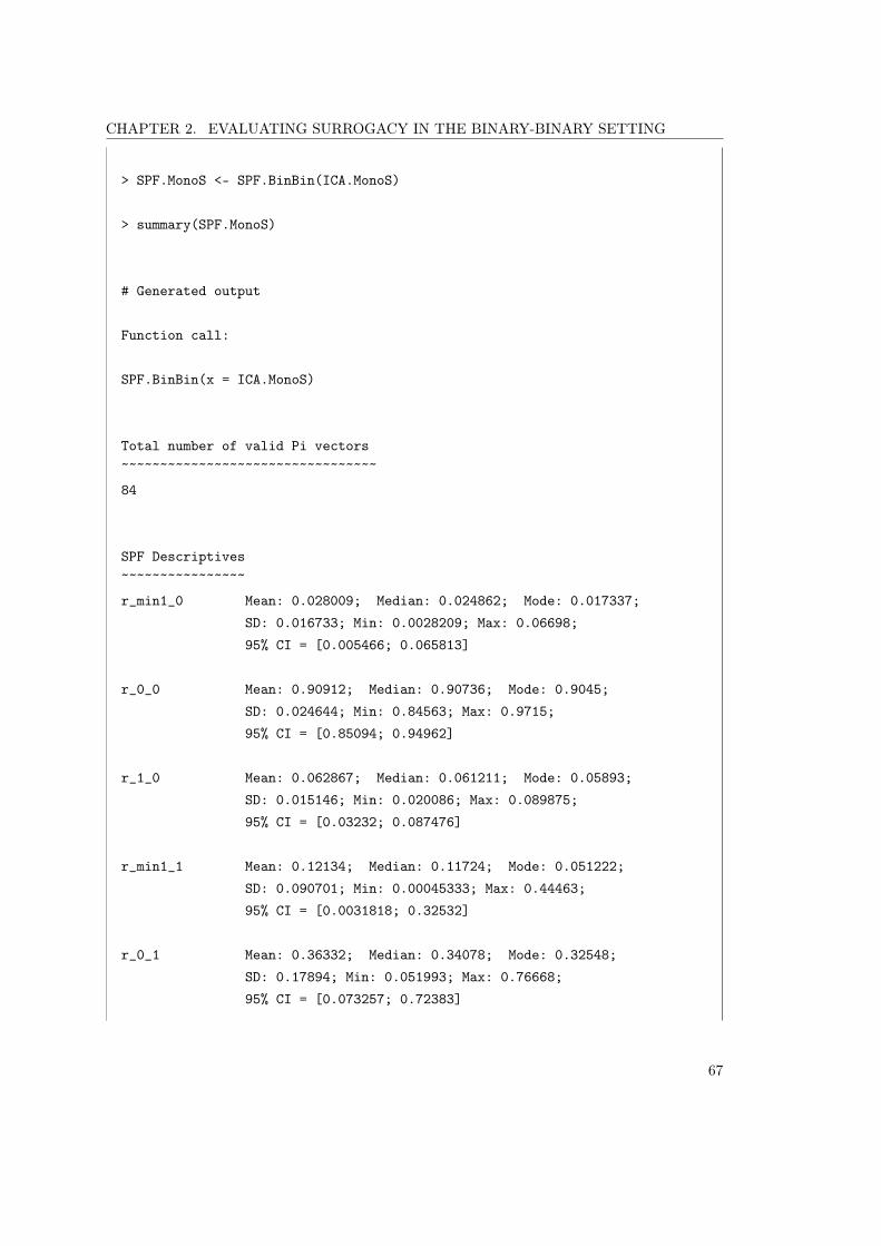
CHAPTER 2. EVALUATING SURROGACY IN THE BINARY-BINARY SETTING
> SPF.MonoS <- SPF.BinBin(ICA.MonoS)
> summary(SPF.MonoS)
# Generated output
Function call:
SPF.BinBin(x = ICA.MonoS)
Total number of valid Pi vectors~~~~~~~~~~~~~~~~~~~~~~~~~~~~~~~~~84
SPF Descriptives~~~~~~~~~~~~~~~~r_min1_0 Mean: 0.028009; Median: 0.024862; Mode: 0.017337;
SD: 0.016733; Min: 0.0028209; Max: 0.06698;95% CI = [0.005466; 0.065813]
r_0_0 Mean: 0.90912; Median: 0.90736; Mode: 0.9045;SD: 0.024644; Min: 0.84563; Max: 0.9715;95% CI = [0.85094; 0.94962]
r_1_0 Mean: 0.062867; Median: 0.061211; Mode: 0.05893;SD: 0.015146; Min: 0.020086; Max: 0.089875;95% CI = [0.03232; 0.087476]
r_min1_1 Mean: 0.12134; Median: 0.11724; Mode: 0.051222;SD: 0.090701; Min: 0.00045333; Max: 0.44463;95% CI = [0.0031818; 0.32532]
r_0_1 Mean: 0.36332; Median: 0.34078; Mode: 0.32548;SD: 0.17894; Min: 0.051993; Max: 0.76668;95% CI = [0.073257; 0.72383]
67

CHAPTER 2. EVALUATING SURROGACY IN THE BINARY-BINARY SETTING
r_1_1 Mean: 0.51534; Median: 0.50723; Mode: 0.47828;SD: 0.18378; Min: 0.1018; Max: 0.92469;95% CI = [0.18044; 0.88129]
> plot(SPF.MonoS)
# Generated output
r(−1, 0)
Frequency
0.0 0.4 0.8
05
1015
r(0, 0)
Frequency
0.0 0.4 0.8
05
1015
2025
30
r(1, 0)Frequency
0.0 0.4 0.8
05
1015
20
r(−1, 1)
Frequency
0.0 0.4 0.8
05
1015
20
r(0, 1)
Frequency
0.0 0.4 0.8
05
1015
r(1, 1)
Frequency
0.0 0.4 0.8
05
1015
Notice that the previous output does not show estimates for r(i, j = �1), as the probabilities ofthese events are 0 when monotonicity for S is assumed.
As can be seen in the top center figure of the plot, the mean br(0, 0) = 0.9091 (range[0.8456; 0.9715]) and, therefore, causal necessity is largely supported in this scenario. However,when there is a positive individual causal treatment effect on S (i.e., �S = 1), there is substan-tial uncertainty with respect to the individual causal treatment effect on T (i.e., �T ; see bottom
68

CHAPTER 2. EVALUATING SURROGACY IN THE BINARY-BINARY SETTING
figures in the plot). Indeed, the mean br(1, 1) = 0.5153 (range [0.1018; 0.9247]) whilst the meanbr(�1, 1) = 0.1213 (range [0.0005; 0.4446]) and mean br(0, 1) = 0.3633 (range [0.0520; 0.7667]).The (mean) probability of correctly predicting �T when �S = 1 is thus roughly equal to the(mean) probability of making an erroneous prediction, i.e., br (1, 1) ⇡ br (�1, 1) + br (0, 1) ⇡ 0.50.
Overall, the results in the monotonicity for S scenario indicate that the amount of informationthat �S conveys with respect to �T is quite low (relatively low R2
H). The SPF results indicatethat a lack of treatment effect on S strongly suggest a lack of treatment effect on T , but a positiveimpact of the treatment on S does not provide strong evidence that there will also be a positiveimpact on T .
2.4 BPRS as a surrogate for CGI
The following R code can be used to analyse whether S = clinically relevant change on the BPRSis a good surrogate for T = clinically relevant change on the PANSS (output not shown):
# Obtain marginal probs for S=BPRS, T=CGI> MarginalProbs(Dataset = Schizo_Bin, Surr = BPRS_Bin,
True = CGI_Bin, Treat = Treat)
# ICA, assume no monotonicity> ICA <- ICA.BinBin.Grid.Sample(pi1_1_=0.0179, pi0_1_=0.4574,pi1_0_=0.3049, pi_1_1=0.0351, pi_1_0=0.2895, pi_0_1=0.5219, Seed=1,Monotonicity=c("No"), M=10000) # Seed is used for reproducibility
# Examine results> summary(ICA)> plot(ICA)
# SPF> SPF <- SPF.BinBin(ICA)
# Examine results> summary(SPF)> plot(SPF)
# Explore impact of monotonicity assumptions
69

CHAPTER 2. EVALUATING SURROGACY IN THE BINARY-BINARY SETTING
# ICA> ICA_mono <- ICA.BinBin.Grid.Sample(pi1_1_=0.0179, pi0_1_=0.4574,pi1_0_=0.3049, pi_1_1=0.0351, pi_1_0=0.2895, pi_0_1=0.5219, Seed=1,Monotonicity=c("General"), M=5000000)
> plot(ICA_mono)> summary(ICA_mono)
# SPF> SPF_mono <- SPF.BinBin(ICA_mono)> summary(SPF_mono)> plot(SPF)
70

Chapter 3
Evaluating predictors of treatment suc-
cess: case study analysis details
3.1 Introduction
In personalized medicine one wants to know, for a given patient and his or her outcomes onpredictor variables, how likely it is that a given treatment will be more beneficial than an al-ternative one. The R package EffectTreat allows for quantifying the predictive causal association(PCA), i.e., the association between the vector of pretreatment predictors and the individualcausal effect of the treatment. Here, it is detailed how the case study analysis results detailed inChapter 5 of Van der Elst (2016) can be replicated using the EffectTreat package.
3.2 The dataset: a clinical trial in opiate/heroin addiction
The data come from a randomized clinical trial in which the clinical utility of buprenorphine/naloxone(experimental treatment) was compared to clonidine (control treatment) for a short-term (13-day) opiate/heroin detoxification treatment. Before and after the treatment, patients were as-sessed for relapse, withdrawal symptoms, and treatment satisfaction (for details, see Section 2.1.2
in Van der Elst, 2016).The vector of potential pretreatment predictors (S) contains craving at screening (S1), the
Clinical Opiate Withdrawal Scale (COWS) score at screening (S2), and heroin use in the 30 daysprior to screening (S3). Craving at screening was measured by means of a visual analogue scale(score range [0; 100]). The COWS is an 11-item interviewer-administered questionnaire designedto provide a description of the signs and symptoms of opiate withdrawal like, e.g., sweating,runny nose, etc; (score range [52; 200]). Higher craving and higher COWS scores are indicativefor more severe heroin addiction.
71

CHAPTER 3. EVALUATING PREDICTORS OF TREATMENT SUCCESS
Table 3.1: Correlations between S1 = craving at screening, S2 = COWS at screening, S3 =heroin use at screening and T = heroin use after treatment in the control (T0) and experimentaltreatment (T1) groups, and significance of the difference of the correlations.
T0 T1 Difference r(Sx, T0) and r(Sx, T1)
S1 �0.029 (p = 0.768) �0.087 (p = 0.190) p = 0.624
S2 �0.334 (p = 0.001) �0.326 (p = 0.001) p = 0.936
S3 0.148 (p = 0.130) 0.185 (p = 0.005) p = 0.749
The number of days that heroin was used in the 30 days prior to the second follow-up (thesecond follow-up took place 3 months after the start of the treatment) was used as the trueendpoint T .
The data are not included in the EffectTreat library as they are not in the public domain.Nonetheless, the data can be downloaded (after registration) from the National Institute on DrugAbuse website (https://www.drugabuse.gov; here, we analyze the combined data of studiesNIDA-CTN-0001 and NIDA-CTN-0002).
Data descriptives Data were available for 335 patients, of whom 106 received the activecontrol clonidine and 229 received the experimental treatment buprenorphine/naloxone. Studydrop-out was substantial: T was observed for 104 patients and missing for 231 patients. Themissing values for T were multiply imputed using M = 1, 000 imputations. The imputationmodel included treatment, the three pretreatment variables S1–S3, and T . The analysis beloware based on the multiply imputed data.
Table 3.1 shows the correlations between the different components of S and T in the activecontrol (T0) and experimental treatment (T1) conditions. The correlations between S1 and T0/T1
close to zero and not significant. The correlations between S2 and T0/T1 were significantlynegative, indicating that patients who had higher COWS scores tended to use less heroin inthe 30-day interval after the treatment in both treatment conditions. On the other hand, thecorrelations between S3 and T0/T1 were positive, which indicates that patients who used moreheroin in the 30-day interval prior to screening also tended to use more heroin in the 30-dayinterval after the treatment. Notice that the correlation between S3 and T was not significant inthe active control treatment group whilst it was significant in the experimental treatment group– albeit the difference between both correlation coefficients was not significant.
72

CHAPTER 3. EVALUATING PREDICTORS OF TREATMENT SUCCESS
3.3 The predictive causal association (PCA; R2
)
After installation of the EffectTreat package in R (using the install.packages(“EffectTreat”)command), the package can be loaded in memory using the command:
> library(EffectTreat)
The function Multivar.PCA.ContCont() implements the sensitivity-based approach to estimateR2 across a set of plausible values for the unidentified correlation ⇢T0T1 (for details, see Chapter
5 of Van der Elst, 2016). This function requires the user to specify the following main arguments:
• Sigma_TT=: the variance-covariance matrix of the true endpoints:
⌃TT =
�T0T0 �T0T1
�T0T1 �T1T1
!.
• Sigma_TS=: the matrix that contains the covariances �T0Sr, �T1Sr. For example, whenthere are 2 pretreatment predictors:
⌃TS =
�T0S1 �T0S2
�T1S1 �T1S2
!.
• Sigma_SS=: the variance-covariance matrix of the pretreatment predictors. For example,when there are 2 pretreatment predictors:
⌃SS =
�S1S1 �S1S2
�S1S2 �S2S2
!.
• T0T1=: a vector (or scalar) that specifies the correlation(s) between the (unidentifiable)counterfactuals T0 and T1 (⇢T0T1). Default seq(-1, 1, by=.01), i.e., the values �1,�0.99, �0.98, ..., 1.
In the opiate/heroin data set, the estimated relevant covariance matrices are:
⌃TT =
82.274 �T0T1
�T0T1 96.386
!,
⌃TS =
�7.266 �61.212 13.281
�25.196 �65.375 17.563
!,
and
⌃SS =
0
BB@
882.352 49.234 6.420
49.234 411.964 �26.205
6.420 �26.205 95.400
1
CCA .
The following command is used to conduct the analysis:
73

CHAPTER 3. EVALUATING PREDICTORS OF TREATMENT SUCCESS
# First define the covariance matrices to be used in the# Multivar.PCA.ContCont() function call> Sigma_TT = matrix(c(82.274, NA, NA, 96.386), byrow=TRUE, nrow=2)
> Sigma_TS = matrix(data = c(-7.266, -61.212, 13.281,-25.196, -65.375, 17.563), byrow = T, nrow = 2)
> Sigma_SS = matrix(data=c(882.352, 49.234, 6.420,49.234, 411.964, -26.205, 6.420, -26.205, 95.400),byrow = T, nrow = 3)
# Compute PCA> Results <- Multivar.PCA.ContCont(Sigma_TT = Sigma_TT,Sigma_TS = Sigma_TS, Sigma_SS = Sigma_SS)
A summary of the results can be obtained by applying the summary() function to the fittedResults object:
> summary(Results)
# Generated output:
Function call:
Multivar.PCA.ContCont(Sigma_TT = Sigma_TT, Sigma_TS = Sigma_TS,Sigma_SS = Sigma_SS)
# Total number of matrices that can be formed by the specified vectors# and/or scalars of the correlations in the function call#~~~~~~~~~~~~~~~~~~~~~~~~~~~~~~~~~~~~~~~~~~~~~~~~~~~~~~~~~~~~~~~~~~~~~~~~
201
# Total number of positive definite matrices#~~~~~~~~~~~~~~~~~~~~~~~~~~~~~~~~~~~~~~~~~~~
174
74

CHAPTER 3. EVALUATING PREDICTORS OF TREATMENT SUCCESS
# Predictive causal association (PCA; R^2_{psi}) results summary#~~~~~~~~~~~~~~~~~~~~~~~~~~~~~~~~~~~~~~~~~~~~~~~
Mean (SD) PCA: 0.0099 (0.0240) [min: 0.0019; max: 0.2470]Mode PCA: 0.0029
Quantiles of the PCA distribution:
5% 10% 20% 50% 80%0.001958460 0.002066354 0.002322228 0.003694800 0.009035708
90% 95%0.017440915 0.032640483
The output shows that out of the 201 matrices that can be formed (based on the specified⌃TT , ⌃TS , ⌃SS and the vector of plausible values for ⇢T0T1), 174 positive-definite matriceswere retained. The subsequent section in the output shows that the mean R2
= 0.0099, modeR2 = 0.0029, and median R2
= 0.0037. Further, 95% of the R2 values were 0.0326 and R2
wasat most 0.2470. These results show that in most ‘realities’ that are compatible with the observeddata, R2
is low. It can thus be concluded that the accuracy by which a patient’s individualcausal treatment effect on T can be predicted based on S is poor. This result exemplifies whatwas stated in Lemma 4 in Chapter 5 of Van der Elst (2016), i.e., that the presence of correlation(see Table 3.1 on page 72) does not guarantee the predictive validity of S with respect to �T .
The plot() function allows to further explore the behavior of estimates of R2 . For example,
plots of the relative frequencies (percentages) and cumulative frequencies can be requested byusing the Type=”Percent” and Type=”CumPerc” arguments in the plot() call:
> plot(Results, Type="Percent") #histogram with percentages
# Generated output:
75

CHAPTER 3. EVALUATING PREDICTORS OF TREATMENT SUCCESS
PCA
Rψ2
Percentage
0.00 0.05 0.10 0.15 0.20 0.25
0.0
0.2
0.4
0.6
0.8
> plot(Results, Type="CumPerc") #cumulative percentages
0.00 0.05 0.10 0.15 0.20 0.25
0.2
0.4
0.6
0.8
1.0
PCA
Rψ2
Cum
ulat
ive p
erce
ntag
e
These plots confirm the earlier claim that R2 is low in the large majority of realities that are
compatible with the observed data.
3.3.1 The relation between ⇢T0T1 and the predictive causal association
(PCA; R2 )
A plot that is useful to examine the impact of the assumptions regarding the unidentified cor-relations ⇢T0T1 on R2
can be obtained using the Effect.T0T1=TRUE argument in the plot()call:
76

CHAPTER 3. EVALUATING PREDICTORS OF TREATMENT SUCCESS
> plot(Results, EffectT0T1=TRUE)
# Generated output:
−0.5 0.0 0.5 1.0
0.00
0.05
0.10
0.15
0.20
0.25
ρT0T1
PCA
As can be seen, R2 increases as a function of ⇢T0T1. Nonetheless, even when ⇢T0T1 is close to 1
the R2 is only about 0.25. A table that contains the ⇢T0T1 and their corresponding R2
that leadto valid results (positive definite ⌃ matrices) can be obtained using the following commands:
> TableResults <- cbind(Results$T0T1, Results$PCA)[order(Results$PCA),]> colnames(TableResults) <- c("T0T1", "PCA")> head(TableResults) # Show lowest PCA values
# Generated output:
T0T1 PCA[1,] -0.74 0.001861259[2,] -0.73 0.001871999[3,] -0.72 0.001882863[4,] -0.71 0.001893853[5,] -0.70 0.001904973[6,] -0.69 0.001916224
> tail(TableResults) # Show highest PCA values
77

CHAPTER 3. EVALUATING PREDICTORS OF TREATMENT SUCCESS
# Generated output:
T0T1 PCA[169,] 0.94 0.05138932[170,] 0.95 0.06106092[171,] 0.96 0.07521695[172,] 0.97 0.09791763[173,] 0.98 0.14024349[174,] 0.99 0.24702061
> TableResults[TableResults[,1]==0] # Show PCA for rho_T0T1=0
# Generated output:
[1] 0.000000000 0.003234288
The output shows that e.g., the highest R2 = 0.2470 (obtained when ⇢T0T1 = 0.99) is about
130 times higher compared to the lowest R2 = 0.0019 (obtained when ⇢T0T1 = �0.74). The
unverifiable assumptions regarding ⇢T0T1 thus have a profound impact on R2 . As another
example, the output shows that R2 = 0.0032 when ⇢T0T1 = 0 (independence).
Given that ⇢T0T1 is not identifiable, based on the data alone one cannot distinguish betweenthese scenarios. Nonetheless, in some applications subject-specific information may be available.This subject-specific information can be easily incorporated into the analysis. For instance, letus assume that, based on expert opinion, ⇢T0T1 < 0.2 is considered to be biologically implausible.A plot of the R2
values that are obtained under ‘biologically plausible’ conditions (⇢T0T1 � 0.2)can be obtained using the commands:
# Make matrix with subgroup of more biologically plausible results
> BiolPlaus <- TableResults[TableResults[,1]>=0.20,]
# Plot PCA based on biologically more plausible assumptions> hist(BiolPlaus[,2], col="grey", xlab="PCA",main="Biologically more plausible results")
# Generated output:
78
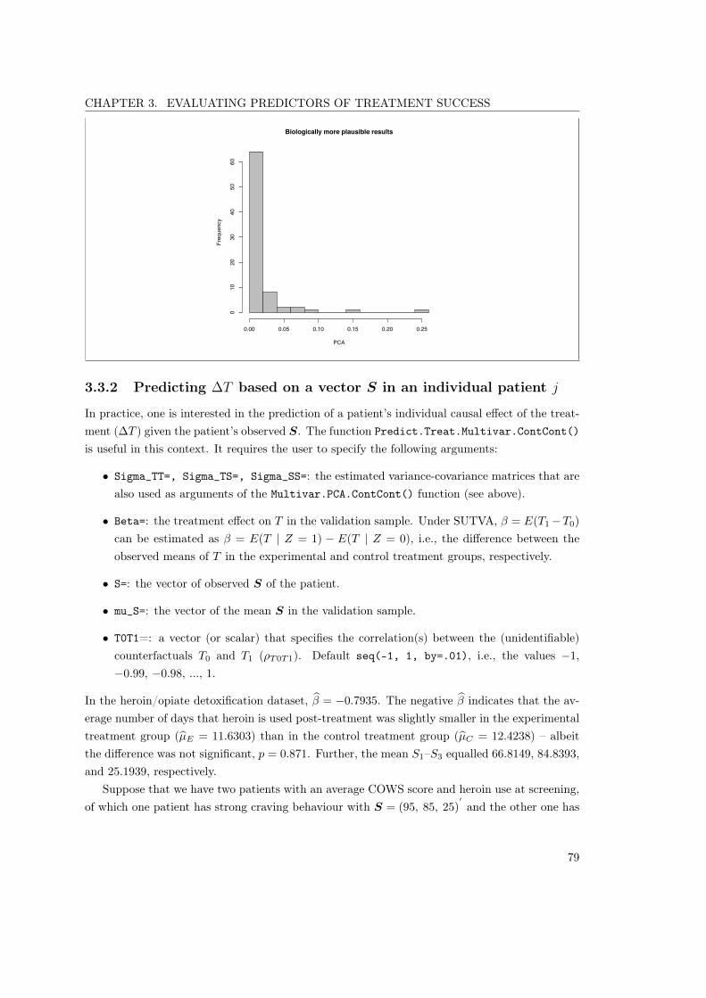
CHAPTER 3. EVALUATING PREDICTORS OF TREATMENT SUCCESS
Biologically more plausible results
PCA
Frequency
0.00 0.05 0.10 0.15 0.20 0.25
010
2030
4050
60
3.3.2 Predicting �T based on a vector S in an individual patient j
In practice, one is interested in the prediction of a patient’s individual causal effect of the treat-ment (�T ) given the patient’s observed S. The function Predict.Treat.Multivar.ContCont()is useful in this context. It requires the user to specify the following arguments:
• Sigma_TT=, Sigma_TS=, Sigma_SS=: the estimated variance-covariance matrices that arealso used as arguments of the Multivar.PCA.ContCont() function (see above).
• Beta=: the treatment effect on T in the validation sample. Under SUTVA, � = E(T1�T0)
can be estimated as � = E(T | Z = 1) � E(T | Z = 0), i.e., the difference between theobserved means of T in the experimental and control treatment groups, respectively.
• S=: the vector of observed S of the patient.
• mu_S=: the vector of the mean S in the validation sample.
• T0T1=: a vector (or scalar) that specifies the correlation(s) between the (unidentifiable)counterfactuals T0 and T1 (⇢T0T1). Default seq(-1, 1, by=.01), i.e., the values �1,�0.99, �0.98, ..., 1.
In the heroin/opiate detoxification dataset, b� = �0.7935. The negative b� indicates that the av-erage number of days that heroin is used post-treatment was slightly smaller in the experimentaltreatment group (bµE = 11.6303) than in the control treatment group (bµC = 12.4238) – albeitthe difference was not significant, p = 0.871. Further, the mean S1–S3 equalled 66.8149, 84.8393,and 25.1939, respectively.
Suppose that we have two patients with an average COWS score and heroin use at screening,of which one patient has strong craving behaviour with S = (95, 85, 25)
0and the other one has
79

CHAPTER 3. EVALUATING PREDICTORS OF TREATMENT SUCCESS
low craving behaviour with S = (5, 85, 25)0. The following code can be used to predict �T for
these patients:
> Beta <- -0.7935 # Specify the treatment effect
# Specify means S_1, S_2, and S_3> mu_S = matrix(c(66.8149, 84.8393, 25.1939), nrow=3)
# Specify the vector of S values for patient with strong craving> S_strong = matrix(c(95, 85, 25), nrow=3)
# Specify the vector of S values for patient with low craving> S_low = matrix(c(5, 85, 25), nrow=3)
# Predict Delta_T based on S# For patient with strong craving> Pred_S_strong <- Predict.Treat.Multivar.ContCont(Sigma_TT=Sigma_TT,Sigma_TS=Sigma_TS, Sigma_SS=Sigma_SS, Beta=Beta,S=S_strong, mu_S=mu_S, T0T1=seq(-1, 1, by=.01))
# For patient with low craving> Pred_S_low <- Predict.Treat.Multivar.ContCont(Sigma_TT=Sigma_TT,Sigma_TS=Sigma_TS, Sigma_SS=Sigma_SS, Beta=Beta, S=S_low, mu_S=mu_S,T0T1=seq(-1, 1, by=.01))
The results can be examined by applying the summary() function to the fitted objects Pred_S_strongand Pred_S_low:
# Results for patient with strong craving> summary(Pred_S_strong)
# Generated output:
Function call:
Predict.Treat.Multivar.ContCont(Sigma_TT = Sigma_TT,Sigma_TS = Sigma_TS, Sigma_SS = Sigma_SS, Beta = Beta,S = S_strong, mu_S = mu_S, T0T1 = seq(-1, 1, by = 0.01))
80

CHAPTER 3. EVALUATING PREDICTORS OF TREATMENT SUCCESS
# Predicted (Mean) Delta_T_j | S_j#~~~~~~~~~~~~~~~~~~~~~~~~~~~~~~~~~
-1.377375
# Variances and 95% support intervals of Delta_T_j | S_j for# different values of rho_T0T1#~~~~~~~~~~~~~~~~~~~~~~~~~~~~~~~~~~~~~~~~~~~~~~~~~~~~~~~~~~~~~~~
rho_T0T1 Var Delta_T_j 95% supp. int.| S_j around Delta_T_j | S_j
(min. value) -0.740 309.877 [-35.87928; 33.12453](max. value) 0.990 1.761 [-3.978588; 1.223839](median value) 0.125 155.819 [-25.84315; 23.0884](mean value) 0.125 155.819 [-25.84315; 23.0884]
# Proportion of 95% support intervals for Delta_T_j | S_jthat include 0, are < 0, and are > 0#~~~~~~~~~~~~~~~~~~~~~~~~~~~~~~~~~~~~~~~~~~~~~~~~~~~~~~~~
0 included in support interval: 1 (obtained for rho_T0T1values in range [-0.74; 0.99])
Entire support interval below 0: 0Entire support interval above 0: 0
# Results for patient with low craving> summary(Pred_S_low)
# Generated output:
Function call:
81

CHAPTER 3. EVALUATING PREDICTORS OF TREATMENT SUCCESS
Predict.Treat.Multivar.ContCont(Sigma_TT = Sigma_TT,Sigma_TS = Sigma_TS, Sigma_SS = Sigma_SS, Beta = Beta,S = S_low, mu_S = mu_S, T0T1 = seq(-1, 1, by = 0.01))
# Predicted (Mean) Delta_T_j | S_j#~~~~~~~~~~~~~~~~~~~~~~~~~~~~~~~~~
0.4567497
# Variances and 95% support intervals of Delta_T_j | S_j for# different values of rho_T0T1#~~~~~~~~~~~~~~~~~~~~~~~~~~~~~~~~~~~~~~~~~~~~~~~~~~~~~~~~~~~~~~~
rho_T0T1 Var Delta_T_j 95% supp. int.| S_j around Delta_T_j | S_j
(min. value) -0.740 309.877 [-34.04516; 34.95866](max. value) 0.990 1.761 [-2.144464; 3.057963](median value) 0.125 155.819 [-24.00902; 24.92252](mean value) 0.125 155.819 [-24.00902; 24.92252]
# Proportion of 95% support intervals for Delta_T_j | S_jthat include 0, are < 0, and are > 0#~~~~~~~~~~~~~~~~~~~~~~~~~~~~~~~~~~~~~~~~~~~~~~~~~~~~~~~~
0 included in support interval: 1 (obtained for rho_T0T1values in range [-0.74; 0.99])
Entire support interval below 0: 0Entire support interval above 0: 0
As can be seen in the output, the expected �T |S for the patients with strong and low cravingbehaviour equal �1.3774 and 0.4567, respectively. Thus, a patient with strong craving behaviouris expected to have about 1.5 more heroin-free days in the post-treatment interval with theexperimental treatment than with the control treatment, whereas the patient with low cravingbehaviour is expected to have about 0.5 more heroin-free days in the post-treatment intervalwith the control treatment compared to with the experimental treatment.
82

CHAPTER 3. EVALUATING PREDICTORS OF TREATMENT SUCCESS
On average, the experimental treatment thus appears to be more effective for patients withstrong craving behaviour whereas the control treatment appears to be more effective for patientswith low craving behaviour. In spite of the previous average predictions, the 95% supportinterval around �T |S for a patient with low craving is [�24.0090; 24.9225] when it is assumedthat ⇢T0T1 = 0.125 (the mean value of ⇢T0T1). Thus, the new treatment may still be a betteroption for some patients with low craving behaviour.
Notice further that the 95% support interval for �T |S narrows when ⇢T0T1 increases. Non-etheless, even when it is assumed that there is a nearly perfect correlation between T1 and T0,there remains a substantial amount of uncertainty in the prediction of the individual causaltreatment effect. For instance, assuming ⇢T0T1 = 0.990, the 95% support interval around �T |Sfor the patient with low craving behavior is [�2.1445; 3.0580]. This level of uncertainty is to beexpected given the negligible value of R2
.The final part of the output provides an overview of the proportion of support intervals for
�T |S that include 0 (inconclusive prediction), that lay entirely below 0 (the experimental treat-ment is more beneficial to the patient), and that lay entirely above 0 (the control treatment ismore beneficial to the patient). As can be seen, the 95% support intervals of �T |S included 0
in all cases for the patients with strong and low craving behavior.
The results can also be graphically depicted by applying the plot() function to the fitted objectsPred_S_strong and Pred_S_low. By default, the distribution of �T |S is shown for the median⇢T0T1 value, i.e., for ⇢T0T1 = 0.125. The following command can be used to obtain the plot forthe patient with strong craving behaviour:
> plot(Pred_S_strong) # Plot for patient with strong craving behaviour
# Generated output:
83

CHAPTER 3. EVALUATING PREDICTORS OF TREATMENT SUCCESS
−40 −20 0 20 40
0.00
0.01
0.02
0.03
0.04
0.05
0.06
∆Tj|Sj
ρT0T1= 0.125
The vertical black dashed line is the expected �T |S value, and the dashed green lines depict the95% support interval. In line with the earlier results, the 95% support interval for �T |S of thepatient with strong craving behaviour assuming ⇢T0T1 = 0.125 contains 0 and thus no significantdifferences between both treatments on T are expected for this patient.
It is also possible to request the 95% support interval for a particular value of ⇢T0T1 by usingthe Specific.T0T1= argument in the plot() call. For example, the 95% support interval around�T |S assuming ⇢T0T1 = 0.7 for the patient with strong craving behaviour can be requested usingthe following command:
> plot(Pred_S_strong, Specific.T0T1=.7) # Plot for patient with strong# craving, rho_T0T1=.7
# Generated output:
84
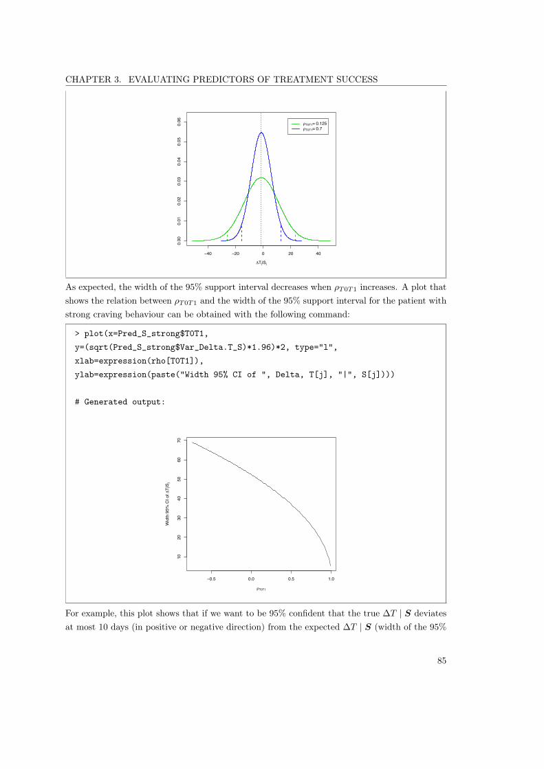
CHAPTER 3. EVALUATING PREDICTORS OF TREATMENT SUCCESS
−40 −20 0 20 40
0.00
0.01
0.02
0.03
0.04
0.05
0.06
∆Tj|Sj
ρT0T1= 0.125ρT0T1= 0.7
As expected, the width of the 95% support interval decreases when ⇢T0T1 increases. A plot thatshows the relation between ⇢T0T1 and the width of the 95% support interval for the patient withstrong craving behaviour can be obtained with the following command:
> plot(x=Pred_S_strong$T0T1,y=(sqrt(Pred_S_strong$Var_Delta.T_S)*1.96)*2, type="l",xlab=expression(rho[T0T1]),ylab=expression(paste("Width 95% CI of ", Delta, T[j], "|", S[j])))
# Generated output:
−0.5 0.0 0.5 1.0
1020
3040
5060
70
ρT0T1
Wid
th 9
5% C
I of ∆
T j|S
j
For example, this plot shows that if we want to be 95% confident that the true �T | S deviatesat most 10 days (in positive or negative direction) from the expected �T | S (width of the 95%
85

CHAPTER 3. EVALUATING PREDICTORS OF TREATMENT SUCCESS
support interval below 20), the assumption that ⇢T0T1 � 0.96 should be reasonable.
A user-friendly scoring sheet The Predict.Treat.Multivar.ContCont() function allowsfor the computation of the expected �T | S and 95% support interval, as illustrated above.However, not all practitioners may be familiar with R (e.g., a medical doctor who is decidingwhich treatment is best for his or her patient). To increase the user-friendliness and the use ofthe methodology in practice, it may be useful to make an Excel sheet (a well-known and widelyavailable software tool) available that conducts all the required computations automatically.
By means of illustration, consider the screen shot shown in Figure 3.12. Here, the user simplyfills-in the observed values for the pretreatment variables S of the patient and the assumedcorrelation ⇢T0T1 in the cells marked in blue. For example, suppose that S1 = 5, S2 = 85, andS3 = 25 (the patient with low craving behaviour in the example above) and it is assumed that⇢T0T1 = 0.125. After filling in these values in the Excel sheet, the output shows the expected�T | S = 0.4567 and 95% support interval [�24.0090; 24.9225]. Further, towards the end of thesheet, the conclusion of the analysis is explicitly stated, i.e., the expected �T for this patient ispositive and thus the control treatment is expected to be more beneficial than the experimentaltreatment though the difference between the treatments is not significant (the 95% supportinterval contains zero).
3.4 Regression-based approach
The methodology used in Section 3.3 of this online Appendix focussed on individual causaltreatment effects. Here, the focus will be on average causal treatment effects (for details, seeGelman and Hill, 2006).
By virtue of the randomisation procedure that was used in the opiate/heroin addiction studyand by assuming SUTVA (i.e., the treatment assignment for one individual does not affect theoutcome of other patients in the study), the average causal treatment effect can be estimated byfitting the following multiple linear regression model:
T = �0 + �1Z +
pX
k=1
↵kSk +
pX
k=1
�kSkZ + " (3.1)
where T is the true endpoint (number of days that a patient uses heroin post-treatment), Z isthe treatment indicator, and Sk are the pretreatment indicators (S1 = craving at screening, S2
= COWS at screening, and S3 = heroin use at screening).Table 3.2 shows the results when model (3.1) is fitted to the data. As can be seen, the
estimated average causal treatment effect is ECE (S) = �1.4429�0.006S1�0.002S2+0.045S3.A modified likelihood-ratio test based on the multiply-imputed datasets (Meng and Rubin, 1992)
2The Excel sheet can be downloaded at https://dl.dropboxusercontent.com/u/8416806/PredictDaysHeroin.xlsx.
86

CHAPTER 3. EVALUATING PREDICTORS OF TREATMENT SUCCESS
Figure 3.1: Excel sheet for user-friendly prediction of �T | S and its 95% support interval.
87

CHAPTER 3. EVALUATING PREDICTORS OF TREATMENT SUCCESS
was conducted to evaluate whether the S by treatment interaction was significant. This was notthe case (Dm = 0.1833, p = 0.908), indicating that S is a poor predictor of the average causaltreatment effect.
Table 3.2: Parameter estimates for regression model (3.1).� s.e. p
Intercept 22.519 6.385 0.001
Z �1.4429 7.134 0.840
S1: craving �0.008 0.040 0.838
S2: COWS �0.143 0.060 0.015
S3: heroin 0.010 0.113 0.378
Z by S1 interaction �0.006 0.046 0.899
Z by S2 interaction �0.002 0.063 0.970
Z by S3 interaction 0.045 0.131 0.729
As was discussed in Section 5.6 of Van der Elst (2016), R2 max and R2
min can be computed basedon � (with �
0= (�1, �2, · · · , �k)) and the variance components ⌃SS , �T0T0 and �T1T1. The
function Min.Max.Multivar.PCA() can be used to compute R2 max and R2
min. This functionrequires the user to specify the following arguments:
• gamma: the vector of the S by treatment interaction coefficients (see model (3.1)).
• Sigma_SS=: the variance-covariance matrix of the pretreatment predictors. For example,
when there are 2 pretreatment predictors, ⌃SS =
�S1S1 �S1S2
�S1S2 �S2S2
!.
• Sigma_T0T0, Sigma_T1T1=: the variances of T in the control and treatment conditions,respectively.
Applied to the heroin case study, the following commands can be used to obtain the results:
# Specify vector of S by treatment interaction coefficients> gamma <- matrix(data = c(-0.006, -0.002, 0.045), ncol=1)
# Specify variances> Sigma_SS = matrix(data=c(882.352, 49.234, 6.420, 49.234, 411.964,-26.205, 6.420, -26.205, 95.400), byrow = T, nrow = 3)Sigma_T0T0 <- 82.274Sigma_T1T1 <- 96.386
88

CHAPTER 3. EVALUATING PREDICTORS OF TREATMENT SUCCESS
# Compute R^2_{psi} min and max> Min.Max.Multivar.PCA(gamma=gamma, Sigma_SS=Sigma_SS,Sigma_T0T0=Sigma_T0T0, Sigma_T1T1=Sigma_T1T1)
# Generated output:
Min PCA: 0.0006419669
Max PCA: 0.4102911
$CallMin.Max.Multivar.PCA(gamma = gamma, Sigma_SS = Sigma_SS,Sigma_T0T0 = Sigma_T0T0, Sigma_T1T1 = Sigma_T1T1)
attr(,"class")[1] "Min.Max.Multivar.PCA"
In line with the results detailed in Section 3.3 (where the (min, max) PCA values were 0.0019
and 0.2470, respectively), R2 min = 0.0006 and R2
max = 0.4102.
89

CHAPTER 3. EVALUATING PREDICTORS OF TREATMENT SUCCESS
90

Chapter 4
Estimating reliability based on lin-
ear mixed-effects models: case study
analysis details
4.1 Introduction
In this chapter, it will be illustrated how the linear mixed-effects model (LMM)-based approachto estimate reliability (for details, see Chapter 7 of Van der Elst, 2016) can be carried-out inpractice using the R package CorrMixed.
In Chapter 7 of Van der Elst (2016), the data of cardiac output experiment (Pikkemaat,Lundin, Stenqvist, Hilgers, and Leonhardt, 2014) were analyzed. The data of the case study arenot in the public domain so they cannot be freely distributed. As an alternative, the data of ahypothetical study that has the same formal characteristics as the Pikkemaat, Lundin, Stenqv-ist, Hilgers, and Leonhardt (2014) study (i.e., the same number of animals, similar correlationstructures in the data, etc.) will be analysed here. Obviously, since we are using data that are
similar but different from the data analyzed in Chapter 7 of Van der Elst (2016), the resultswill also differ.
4.2 The dataset: a simulated study
The data of the fictitious study are included in the R package CorrMixed. The dataset contains360 observations on 5 variables:
• ‘Id’: the animal identifier. There are 10 animals in the dataset.
91

CHAPTER 4. ESTIMATING RELIABILITY
• ‘Cycle’: similarly to what was the case in the Pikkemaat, Lundin, Stenqvist, Hilgers,and Leonhardt (2014) study, the same experiment is repeated multiple times in the sameanimal. Cycle refers to the nth repetition of the experiment (min. = 1, max. = 4).
• ‘Condition’: the experimental condition under which the outcome was measured. Thereare at most 16 experimental conditions within a cycle (similar to the different levels ofPEEP in the Pikkemaat, Lundin, Stenqvist, Hilgers, and Leonhardt, 2014 study).
• ‘Time’: the time point at which the outcome was measured (min. = 1, max. = 47). It isassumed that the time between two successive measurement moments is the same.
• ‘Outcome’: a continuous outcome.
The data are in the ‘long’ format, which means that there are multiple rows for each animal, i.e.,one row for each time the outcome was measured. For example, the first three rows in the datafile look like this:
Id Cycle Condition Time Outcome
1 1 1 1 117.554
1 1 2 2 113.738
1 1 3 3 108.160... ... ... ... ...
After installation of the CorrMixed package in R (using the install.packages(’CorrMixed’)command), the following code is used to load the package and the data of the fictitious casestudy into memory:
> library(CorrMixed) # load the package> data(Example.Data) # load the data> Example.Data[1:5,] # have a look at the first five data rows
# Generated output:Id Cycle Condition Time Outcome
1 1 1 1 1 117.542 1 1 2 2 113.743 1 1 3 3 108.164 1 1 4 4 91.965 1 1 5 5 67.60
Exploratory data analysis A plot of the individual profiles for all animals and the meanevolution over time can be obtained using the Spaghetti.Plot() function of the CorrMixed
package. This function requires the following arguments:
92

CHAPTER 4. ESTIMATING RELIABILITY
• Dataset= : the name of the dataset.
• Outcome=, Id=, Time= : the names of the outcome, subject indicator (Id) and time variables.
By default, the individual profiles and the overall mean are provided. The following commandcan be used to obtain a spaghetti plot for the case study data:
> Spaghetti.Plot(Dataset=Example.Data, Outcome="Outcome", Id="Id",Time="Time")
# Generated output:
0 10 20 30 40
050
100
150
200
250
Time
Outcome
Other options are possible, for example, a plot that shows the median (rather than the mean)and no individual profiles can be requested using the command:
> Spaghetti.Plot(Dataset=Example.Data, Outcome="Outcome", Id="Id",Time="Time", Add.Profiles=FALSE, Add.Mean=FALSE, Add.Median=TRUE)
# Generated output:
93

CHAPTER 4. ESTIMATING RELIABILITY
0 10 20 30 40
050
100
150
200
250
Time
Outcome
4.3 Estimating reliability using linear mixed-effects models
4.3.1 The mean structure of the model
As was also the case with the ZSV outcome (see Chapter 7 in Van der Elst, 2016), the plotsindicate that the relation between time and the outcome is quite complex and cannot be modelledin a straightforward way by using e.g., linear or quadratic polynomials. Therefore, fractionalpolynomials will be considered. The function Fract.Poly() of the CorrMixed package is usefulin this respect. It requires the following arguments:
• Covariate=, Outcome=, Dataset= : the names of the covariate, outcome, and dataset.
• S=: the set that specifies the powers that will be considered in the different models. Bydefault, S = {�2, �1, �0.5, 0, 0.4, 1, 2, 3}.
• Max.M=: the maximum order to be considered for the fractional polynomials.
Here, we request an analysis using the standard set S and m = 3, i.e., fractional polynomials oforder 1, 2, and 3 will be considered:
> FP <- Fract.Poly(Covariate="Time", Outcome="Outcome",Dataset=Example.Data, S=c(-2,-1,-0.5,0,0.5,1,2,3), Max.M=3)
The results can be examined by applying the summary() function to the fitted object FP:
> summary(FP)
# Generated output:
94

CHAPTER 4. ESTIMATING RELIABILITY
Best fitting model for m=1:power1 AIC
-0.5 2715.0
Best fitting model for m=2:power1 power2 AIC
-2 -2 2714
Best fitting model for m=3:power1 power2 power3 AIC
3 3 2 2702
As can be seen, the model of order m = 3 is preferred based on the AIC (a lower AIC is indicativefor a better model fit). This model includes the powers p1 = 3, p2 = 3, and p3 = 2. Recall that�1tp1
+ �2tp1log(t) when p1 = p2. Thus, the mean relation between time and the outcome will
be modelled as �1t2 + �2t3 + �3t3 log(t) (with t = time) when the LMMs are fitted to estimatereliability. In addition, cycle and condition are added as covariates in all models (coded asdummies).
To examine the fit of the model graphically, the following commands can be used:
# Code the predictors for fractional poly (powers: 3, 3, 2)term1 <- Example.Data$Time**3term2 <- (Example.Data$Time**3) * log(Example.Data$Time)term3 <- Example.Data$Time**2
# Plot the mean outcome as function of time# (using the Spaghetti.Plot() function described above)Spaghetti.Plot(Dataset=Example.Data, Outcome="Outcome", Time="Time",Id="Id", Add.Profiles=FALSE, Lwd.Me=1, ylab="Mean Outcome")
# Fit the fractional poly of m=3Model <- lm(Outcome~term1+term2+term3, data=Example.Data)
# Code x=time for plot (for time points 1 -- 47; 47 is max. timein the dataset)time <- 1:47; term1 <- time**3term2 <- (time**3) * log(time)term3 <- time**2
# Predict the outcome at times 1--47 based on the model
95

CHAPTER 4. ESTIMATING RELIABILITY
pred <- Model$coef[1] + (Model$coef[2] * term1) +(Model$coef[3] * term2) + (Model$coef[4] * term3)
# Add the predicted values and a legend to the plotlines(x = 1:47, y=pred, lty=2)legend("topright", c("Observed", "Predicted"), lty=c(1, 2))
# Generated output:
0 10 20 30 40
050
100
150
200
250
Time
Mea
n O
utco
me
ObservedPredicted
4.3.2 The covariance structure of the model
As was also the case in Chapter 7 of Van der Elst (2016), three models with a different covariancestructure will be fitted to the example data to estimate the reliabilities R: (i) Model 1, which is arandom intercept model, (ii) Model 2, which is a random intercept model that includes Gaussianserial correlation, and (iii) Model 3, which is a model that contains a random intercept, slope,and serial correlation.
These models can be fitted in a straightforward way using the WS.Corr.Mixed() function,which has the following main arguments:
• Fixed.Part= : the fixed part of the LMM that has to be fitted to the data, i.e., a for-mula in the form of Outcome ~ Covariate_1 + ... + Covariate_n. The specificationof the argument should be in line with the requirements of the lme function (from thenlme package) that is used to fit the LMMs. To avoid problems with the lme functioncall, do not specify powers directly in the function call. For example, ratherthan specifying Fixed.Part=Outcome~ Time + Time**2 in the function call, first makethe new variable Time squared and add it to the dataset (e.g., Example.Data$TimeSq2 <-
96

CHAPTER 4. ESTIMATING RELIABILITY
Dataset$Time ** 2). Subsequently use the new variable TimeSq2 in the function call ofthe WS.Corr.Mixed() function (e.g., Fixed.Part=Outcome ~ Time + TimeSq).
• Random.Part= : the random part of the model (specified in line with the requirements ofthe lme function, see link provided above for more details).
• Correlation= : the serial correlation component (specified in line with the requirementsof the lme function, see link provided above for more details).
• Dataset=, Id= : the name of the dataset and the subject (Id) indicator.
• Number.Bootstrap= : the number of bootstrap samples that should be used to determinethe confidence interval for R.
• Alpha= : the ↵-level to be used in the bootstrap.
• Model= : the model that should be fitted (Model 1, 2, or 3).
• Time= : the time indicator, default Time=Time. In the current dataset, Time= does not hasto be specified because the time indicator is coded as the default.
4.3.2.1 Model 1
The following commands can be used to fit Model 1 (a random intercept model) to the exampledata (runtime about 5 seconds):
# First code the predictors for time (based on fractional poly# analyses above)> Example.Data$Time2 <- Example.Data$Time**2> Example.Data$Time3 <- Example.Data$Time**3> Example.Data$Time3_log <- (Example.Data$Time**3) *(log(Example.Data$Time))
# Fit Model 1Model1 <- WS.Corr.Mixed(Fixed.Part=Outcome ~ Time2 + Time3 +Time3_log + as.factor(Cycle) + as.factor(Condition),Random.Part = ~ 1|Id, Dataset=Example.Data, Model=1, Id="Id",Number.Bootstrap = 100, Seed = 12345) # Seed for reproducibility
The results can be explored by applying the summary() function to the fitted Model1 object:
> summary(Model1)
# Generated output:
97

CHAPTER 4. ESTIMATING RELIABILITY
Function call:
WS.Corr.Mixed(Dataset = Example.Data, Fixed.Part = Outcome ~Time2 + Time3 + Time3_log + as.factor(Cycle) +as.factor(Condition),
Random.Part = ~1 | Id, Id = "Id", Model = 1,Number.Bootstrap = 100, Seed = 12345)
Model 1, Random intercept=========================
Fitted variance components:---------------------------D: 851.9Sigma**2: 868.7
Estimated correlations R (r(time_j, time_k) constant):------------------------------------------------------R: 0.495195% confidence interval (bootstrap): [0.1594; 0.7331]
Model fit:----------LogLik: -1694AIC: 3436
The relevant variance components are shown at the top of the output, i.e., bd = 851.912 andc�2
= 868.672. Below that, the estimated reliability coefficient is provided. Model 1 assumesthat the reliability for measurements taken at any two measurements is constant, i.e., bR = 0.495
here. The bootstrap based 95% Confidence Interval (CI) is [0.159; 0.733], indicating that thereis substantial uncertainty in the estimated R (which is not surprising given the small amount ofsubjects). Towards the end of the output, model fit statistics are provided, i.e., log likelihood =�1694.042 and AIC = 3436.083. These quantities are useful to compare the fit of Models 1–3(see below below).
A plot of the results can be obtained by applying the plot() function to the fitted objectModel1. By default, the estimated bR (solid line) and 95% CI (dashed lines) is provided:
> plot(Model1)
98

CHAPTER 4. ESTIMATING RELIABILITY
# Generated output:
0 10 20 30 40
−1.0
−0.5
0.0
0.5
1.0
Model 1
Measurement moment
Rel
iabi
lity
4.3.2.2 Model 2
Model 2 adds a Gaussian serial correlation component to the random intercept model. Thefollowing command can be used to fit the model (runtime about 2 minutes):
> Model2 <- WS.Corr.Mixed(Fixed.Part=Outcome ~ Time2 + Time3 +Time3_log + as.factor(Cycle) + as.factor(Condition),Random.Part = ~ 1|Id, Correlation=corGaus(form= ~ Time,nugget = TRUE), Dataset=Example.Data,Model=2, Id="Id", Number.Bootstrap = 100, Seed = 12345)
The results can be explored by applying the summary() function to the fitted Model2 object(restricted output marked by (...)):
> summary(Model2)
# Generated output:
Function call:
WS.Corr.Mixed(Dataset = Example.Data, Fixed.Part = Outcome ~Time2 + Time3 + Time3_log + as.factor(Cycle) +
as.factor(Condition), Random.Part = ~1 | Id,Correlation = corGaus(form = ~Time, nugget = TRUE),Id = "Id", Model = 2, Number.Bootstrap = 100, Seed = 12345)
99

CHAPTER 4. ESTIMATING RELIABILITY
Model 2, Random intercept + serial corr (Gaussian)==================================================
Fitted variance components:---------------------------D: 501Sigma**2: 190.1Tau**2: 893Rho: 3.63
Estimated correlations R as a function of time lag:---------------------------------------------------[1] 0.8388 0.7324 0.6010 0.4837 0.4008 0.3530 0.3299 0.3206[9] 0.3175 0.3165 0.3163 0.3163 0.3163 0.3163 0.3163 0.3163
(...)[41] 0.3163 0.3163 0.3163 0.3163 0.3163 0.3163 0.3163
95% confidence intervals (bootstrap), lower bounds:---------------------------------------------------[1] 7.525e-01 5.786e-01 3.711e-01 2.033e-01 9.182e-02[6] 3.476e-02 1.105e-02 2.951e-03 6.609e-04 1.242e-04
(...)[46] 1.272e-08 1.272e-08
95% confidence intervals (bootstrap), upper bounds:---------------------------------------------------[1] 0.9128 0.8568 0.7866 0.7244 0.6809 0.6562 0.6445 0.6390[9] 0.6365 0.6356 0.6353 0.6353 0.6352 0.6352 0.6352 0.6352
(...)[41] 0.6352 0.6352 0.6352 0.6352 0.6352 0.6352 0.6352
Model fit:----------LogLik: -1567AIC: 3187
The fitted variance components are shown at the top of the output, i.e., bd = 500.966, c�2=
100

CHAPTER 4. ESTIMATING RELIABILITY
190.087, b⌧2 = 893.005, and b⇢ = 3.630. Based on these components, the reliabilities can beestimated as a function of time lag, i.e., bR (ukl). These estimated reliabilities and their bootstrap-based 95% CIs are provided below the variance components in the output (restricted output). Forexample, bR (ukl = 0) = 0.839 with corresponding CI95% = [0.753; 0.913] and bR (ukl = 1) = 0.732
with corresponding CI95% = [0.579; 0.857]. The results can be graphically shown by applyingthe plot() function to the fitted object Model2. By default, the estimated bR (u) (solid line) andthe corresponding 95% CIs (dashed lines) are shown:
> plot(Model2)
# Generated output:
0 10 20 30 40
−1.0
−0.5
0.0
0.5
1.0
Model 2
Time lag
Rel
iabi
lity
The plot shows (i) that bR (u) declines as a function of time lag until it remains essentially constantat about time lag ukl = 10, and (ii) that the CIs are more narrow for shorter time lags and widenfor larger time lags until they remain constant at about time lag ukl = 10.
The argument All.Individual = TRUE of the plot() function can be used to request theestimated R for all pairs of measurement moments (rather than as a function of time lag):
> plot(Model2, All.Individual = TRUE)
# Generated output:
101

CHAPTER 4. ESTIMATING RELIABILITY
0 10 20 30 40
−1.0
−0.5
0.0
0.5
1.0
Model 2
Measurement moment
Rel
iabi
lity
The utmost left line depicts the estimated reliabilities between t1 and all other measurementmoments, the line next to that one depicts the correlations between t2 and measurement moments2–45, etc. This plot illustrates that in Model 2 the estimated reliabilities indeed only depend ofthe time lag (all curves are parallel).
4.3.2.3 Model 3
In Model 3, a random slope for time is added to the LMM. The model can be fitted to the datausing the following command (runtime about 6 minutes):
> Model3 <- WS.Corr.Mixed(Fixed.Part=Outcome ~ Time2 + Time3 +Time3_log + as.factor(Cycle) + as.factor(Condition),Random.Part = ~ 1 + Time|Id,Correlation=corGaus(form= ~ Time, nugget = TRUE),Dataset=Example.Data, Model=3, Id="Id",Number.Bootstrap = 100, Seed = 12345)
Again, the results can be explored by applying the summary() function to the fitted objectModel3. However, Model 3 yields estimated reliabilities for each pair of measurement moments.In the current dataset, the estimated correlation matrix R (tk, tj) is very large because of thelarge number of measurement moments. To avoid large amounts of output, the summary()function is not used here and instead only selected output is requested.
A list with all the components in the fitted object Model3 can be obtained by applying thenames() function:
> names(Model3)
102

CHAPTER 4. ESTIMATING RELIABILITY
# Generated output:
[1] "Model" "D" "Tau2"[4] "Rho" "Sigma2" "AIC"[7] "LogLik" "R" "CI.Upper"
[10] "CI.Lower" "Alpha" "Coef.Fixed"[13] "Std.Error.Fixed" "Time" "Call"
The contents of these components is described in the CorrMixed manual. For example, thecomponents LogLik and AIC contain the model fit statistics. Here, we are primarily interestedin the variance components. These can be requested using the commands:
> Model3$D # D matrix
# Generated output:
[,1] [,2][1,] 1951.73 -62.578[2,] -62.58 2.462
> Model3$Sigma2 # Sigma**2
# Generated output:
[1] 187.5
> Model3$Tau2 # Tau**2
# Generated output:
[1] 578.8
> Model3$Rho # Rho
# Generated output:
[1] 3.18
103

CHAPTER 4. ESTIMATING RELIABILITY
As shown in the output, bD =
1951.732 �62.578
�62.578 2.462
!, c�2
= 187.503, b⌧2 = 578.818, and
b⇢ = 3.180. The estimated reliabilities between all measurement moments and their CIs canbe obtained using the Model3$R, Model3$CI.Upper, and Model3$CI.Lower commands. Forexample, the estimated reliabilities between measurement moments 1–5 and their 95% CIs canbe obtained using the commands:
> Model3$R[1:5,1:5] # Estimated reliabilities t_1 - t_5
# Generated output:
[,1] [,2] [,3] [,4] [,5][1,] 0.9278 0.9044 0.8471 0.7795 0.7222[2,] 0.9044 0.9243 0.8998 0.8398 0.7688[3,] 0.8471 0.8998 0.9207 0.8950 0.8321[4,] 0.7795 0.8398 0.8950 0.9169 0.8900[5,] 0.7222 0.7688 0.8321 0.8900 0.9129
> Model3$CI.Upper[1:5,1:5] # Upper bound CIs
# Generated output:[,1] [,2] [,3] [,4] [,5]
[1,] 0.9557 0.9419 0.9122 0.8775 0.8417[2,] 0.9419 0.9538 0.9383 0.9069 0.8701[3,] 0.9122 0.9383 0.9525 0.9344 0.9013[4,] 0.8775 0.9069 0.9344 0.9518 0.9313[5,] 0.8417 0.8701 0.9013 0.9313 0.9511
> Model3$CI.Lower[1:5,1:5] # Lower bound CIs
# Generated output:
[,1] [,2] [,3] [,4] [,5][1,] 0.8257 0.7618 0.5832 0.3736 0.2003[2,] 0.7618 0.8327 0.7618 0.5832 0.3736[3,] 0.5832 0.7618 0.8327 0.7634 0.5832
104
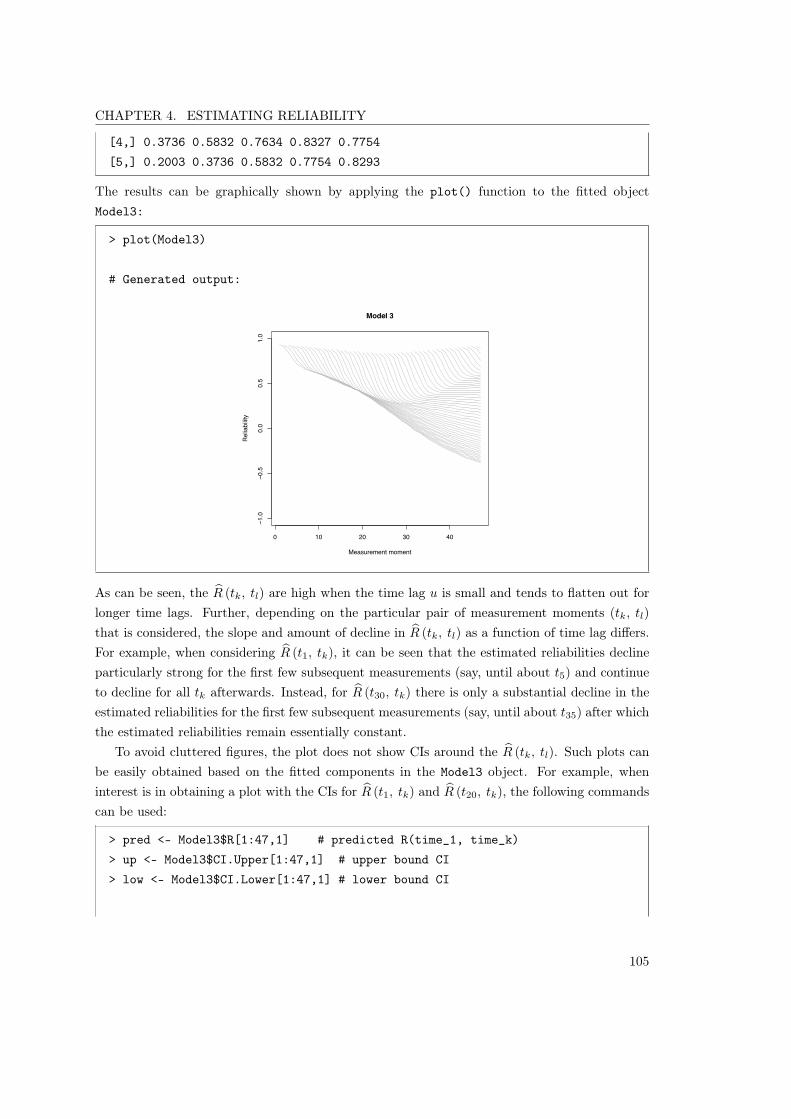
CHAPTER 4. ESTIMATING RELIABILITY
[4,] 0.3736 0.5832 0.7634 0.8327 0.7754[5,] 0.2003 0.3736 0.5832 0.7754 0.8293
The results can be graphically shown by applying the plot() function to the fitted objectModel3:
> plot(Model3)
# Generated output:
0 10 20 30 40
−1.0
−0.5
0.0
0.5
1.0
Model 3
Measurement moment
Rel
iabi
lity
As can be seen, the bR (tk, tl) are high when the time lag u is small and tends to flatten out forlonger time lags. Further, depending on the particular pair of measurement moments (tk, tl)
that is considered, the slope and amount of decline in bR (tk, tl) as a function of time lag differs.For example, when considering bR (t1, tk), it can be seen that the estimated reliabilities declineparticularly strong for the first few subsequent measurements (say, until about t5) and continueto decline for all tk afterwards. Instead, for bR (t30, tk) there is only a substantial decline in theestimated reliabilities for the first few subsequent measurements (say, until about t35) after whichthe estimated reliabilities remain essentially constant.
To avoid cluttered figures, the plot does not show CIs around the bR (tk, tl). Such plots canbe easily obtained based on the fitted components in the Model3 object. For example, wheninterest is in obtaining a plot with the CIs for bR (t1, tk) and bR (t20, tk), the following commandscan be used:
> pred <- Model3$R[1:47,1] # predicted R(time_1, time_k)> up <- Model3$CI.Upper[1:47,1] # upper bound CI> low <- Model3$CI.Lower[1:47,1] # lower bound CI
105

CHAPTER 4. ESTIMATING RELIABILITY
> plot(pred, col=0, ylim=c(-1, 1), xlab="Time", ylab="Reliability",main=expression(paste("Estimated R(", t[1], ", ", t[k], ")", sep="")))> lines(pred) # add predicted R(time_1, time_j)> lines(up, lty=2) # add upper bound CI> lines(low, lty=2) # add lower bound CI
# Generated output:
0 10 20 30 40
−1.0
−0.5
0.0
0.5
1.0
Estimated R(t1, tk)
Time
Rel
iabi
lity
> pred2 <- Model3$R[20:47,20] # predicted R(time_20, time_k)> up2 <- Model3$CI.Upper[20:47,20] # upper bound CI> low2 <- Model3$CI.Lower[20:47,20] # lower bound CI
> plot(pred, col=0, ylim=c(-1, 1), xlab="Time", ylab="Reliability",main=expression(paste("Estimated R(", t[20], ", ", t[k], ")", sep="")))> lines(pred2, x=c(20:47)) # add predicted R(time_20, time_j)> lines(up2, x=c(20:47), lty=2) # add upper bound CI> lines(low2, x=c(20:47), lty=2) # add lower bound CI# Generated output:
106

CHAPTER 4. ESTIMATING RELIABILITY
0 10 20 30 40
−1.0
−0.5
0.0
0.5
1.0
Estimated R(t20, tk)
Time
Rel
iabi
lity
4.3.2.4 Selecting the most appropriate model
The function Model.Fit() can be used to compare Models 1–3 using a likelihood ratio test(using a mixture of �2 distributions to compute the correct p-value when necessarily, for detailssee Verbeke & Molenberghs, 2000):
# compare models 1 and 2> Model.Fit(Model.1 = Model1, Model.2 = Model2)
# Generated output:
Compare Models:=================G2: 253.3003p-value: 9.920398e-56
# compare models 2 and 3> Model.Fit(Model.1 = Model3, Model.2 = Model3)
# Generated output:
Compare Models:=================G2: 14.76563
107

CHAPTER 4. ESTIMATING RELIABILITY
p-value: 0.0003717904
As shown, Model 2 fits the data significantly better than Model 1, and Model 3 fits the datasignificantly better than Model 2. Model 3 would thus be preferred if we would solely rely onstatistical arguments, but considerations of practical usefulness should also be taken into account.For example, in the paper that accompanies this Web Appendix Model 3 also had the best fitwith the data but Model 2 was nonetheless preferred because it provides a more parsimoniousresult.
108

Bibliography
Buyse, M., and Molenberghs, G. (1998). The validation of surrogate endpoints in randomizedexperiments. Biometrics, 54, 1014–1029.
Burzykowski, T., Molenberghs, G., and Buyse, M. (2005). The Evaluation of Surrogate End-
points. New York: Springer-Verlag.
Frangakis, C. E. and Rubin, D. B. (2002). Principal stratification in causal inference. Biometrics,
58, 21–29.
Gelman, A., and Hill, J. (2006). Data analysis using regression and multilevel/hierarchical models.Cambridge: Cambridge University Press.
Guy, W. (1976). ECDEU Assessment Manual for Psychopharmacology - Revised. Rockville, MD:U.S. Department of Health, Education, and Welfare.
Kane, J., Honigfeld, G., Singer, J., and Meltzer, H. (1988). Clozapine for the treatment-resistantschizophrenic. A double-blind comparison with chlorpromazine. Archives of General Psychi-
atry, 45, 789–796.
Kutner, M. H., Nachtsheim, C. J., Neter, J., and Li, W. (2005). Applied linear statistical models
(5th ed.). New York: McGraw Hill.
Leucht, S., Kane, J. M., Kissling, W., Hamann, J., Etschel, E., and Engel, R. (2005). Clinicalimplications of the Brief Psychiatric Rating Scale Scores. British Journal of Psychiatry, 187,366–371.
Meng, X., and Rubin, D. B. (1992). Performing likelihood ratio tests with multiply-imputed datasets. Biometrika, 79, 103-111.
Overall, J., and Gorham, D. (1962). The Brief Psychiatric Rating Scale. Psychological Reports,
10, 799–812.
109

BIBLIOGRAPHY
Pikkemaat, R., Lundin, S., Stenqvist, O., Hilgers, R. D., and Leonhardt, S. (2014). Recentadvances in and limitations of cardiac output monitoring by means of electrical impedancetomography. Anesthesia & Analgesia, 119(1), 76–83.
Singh, M., and Kay, S. (1975). A comparative study of haloperidol and chlorpromazine in termsof clinical effects and therapeutic reversal with benztropine in schizophrenia. Theoretical im-plications for potency differences among neuroleptics. Psychopharmacologia, 43, 103–113.
Tibaldi, F. S., Cortiñas Abrahantes, J., Molenberghs, G., Renard, D., Burzykowski, T., Buyse,M., Parmar, M., Stijnen, T., and Wolfinger, R. (2003). Simplified hierarchical linear modelsfor the evaluation of surrogate endpoints. Journal of Statistical Computation and Simulation,
73, 643–658.
Van der Elst, W. (2016). Statistical Evaluation Methodology for Surrogate Endpoints in Clinical
Studies and Related Topics. Unpublished doctoral dissertation.
Verbeke, G., and Molenberghs, G. (2000). Linear Mixed Models for Longitudinal Data. New York:Springer-Verlag.
110