statistical machine learning for nlppages.cs.wisc.edu/~jerryzhu/pub/zhuccfadl46.pdfstatistical...
TRANSCRIPT

Statistical Machine Learning for NLP
Xiaojin Zhu
[email protected] of Computer Sciences
University of Wisconsin–Madison, USA
CCF/ADL46 2013
Zhu (Univ. Wisconsin) Statistical Machine Learning for NLP CCF/ADL46 2013 1 / 125

Outline
1 Basics of Statistical LearningProbabilityStatistical EstimationRegularizationDecision Theory
2 Graphical ModelsDirected Graphical Models (Bayesian Networks)Undirected Graphical Models (Markov Random Fields)Factor GraphMarkov Chain Monte CarloBelief PropagationMean Field AlgorithmMaximizing Problems (Viterbi)
3 Bayesian Non-Parametric ModelsDirichlet Processes
Zhu (Univ. Wisconsin) Statistical Machine Learning for NLP CCF/ADL46 2013 2 / 125

Basics of Statistical Learning
Outline
1 Basics of Statistical LearningProbabilityStatistical EstimationRegularizationDecision Theory
2 Graphical ModelsDirected Graphical Models (Bayesian Networks)Undirected Graphical Models (Markov Random Fields)Factor GraphMarkov Chain Monte CarloBelief PropagationMean Field AlgorithmMaximizing Problems (Viterbi)
3 Bayesian Non-Parametric ModelsDirichlet Processes
Zhu (Univ. Wisconsin) Statistical Machine Learning for NLP CCF/ADL46 2013 3 / 125

Basics of Statistical Learning Probability
Outline
1 Basics of Statistical LearningProbabilityStatistical EstimationRegularizationDecision Theory
2 Graphical ModelsDirected Graphical Models (Bayesian Networks)Undirected Graphical Models (Markov Random Fields)Factor GraphMarkov Chain Monte CarloBelief PropagationMean Field AlgorithmMaximizing Problems (Viterbi)
3 Bayesian Non-Parametric ModelsDirichlet Processes
Zhu (Univ. Wisconsin) Statistical Machine Learning for NLP CCF/ADL46 2013 4 / 125

Basics of Statistical Learning Probability
Probability
The probability of a discrete random variable A taking the value a isP (A = a) ∈ [0, 1].
Sometimes written as P (a) when no danger of confusion.
Normalization∑
all a P (A = a) = 1.
Joint probability P (A = a,B = b) = P (a, b), the two events bothhappen at the same time.
Marginalization P (A = a) =∑
all b P (A = a,B = b), “summing outB”.
Conditional probability P (a|b) = P (a,b)P (b) , a happens given b happened.
The product rule P (a, b) = P (a)P (b|a) = P (b)P (a|b).
Zhu (Univ. Wisconsin) Statistical Machine Learning for NLP CCF/ADL46 2013 5 / 125

Basics of Statistical Learning Probability
Bayes Rule
Bayes rule P (a|b) = P (b|a)P (a)P (b) .
In general, P (a|b, C) = P (b|a,C)P (a|C)P (b|C) where C can be one or more
random variables.
Bayesian approach: when θ is model parameter, D is observed data,we have
p(θ|D) =p(D|θ)p(θ)p(D)
,
I p(θ) is the prior,I p(D|θ) the likelihood function (of θ, not normalized:
∫p(D|θ) dθ 6= 1),
I p(D) =∫p(D|θ)p(θ) dθ the evidence,
I p(θ|D) the posterior.
Zhu (Univ. Wisconsin) Statistical Machine Learning for NLP CCF/ADL46 2013 6 / 125

Basics of Statistical Learning Probability
Independence
The product rule can be simplified as P (a, b) = P (a)P (b) iff A andB are independent
Equivalently, P (a|b) = P (a), P (b|a) = P (b).
Zhu (Univ. Wisconsin) Statistical Machine Learning for NLP CCF/ADL46 2013 7 / 125

Basics of Statistical Learning Probability
Probability density
A continuous random variable x has a probability density function(pdf) p(x) ∈ [0,∞].
p(x) > 1 is possible! Integrates to 1.∫ ∞−∞
p(x) dx = 1
P (x1 < X < x2) =∫ x2x1p(x) dx
Marginalization p(x) =∫∞−∞ p(x, y) dy
Zhu (Univ. Wisconsin) Statistical Machine Learning for NLP CCF/ADL46 2013 8 / 125

Basics of Statistical Learning Probability
Expectation and Variance
The expectation (“mean” or “average”) of a function f under theprobability distribution P is
EP [f ] =∑a
P (a)f(a)
Ep[f ] =
∫xp(x)f(x) dx
In particular if f(x) = x, this is the mean of the random variable x.
The variance of f is
Var(f) = E[(f(x)− E[f(x)])2] = E[f(x)2]− E[f(x)]2
The standard deviation is std(f) =√
Var(f).
Zhu (Univ. Wisconsin) Statistical Machine Learning for NLP CCF/ADL46 2013 9 / 125

Basics of Statistical Learning Probability
Multivariate Statistics
When x, y are vectors, E[x] is the mean vector
Cov(x, y) is the covariance matrix with i, j-th entry beingCov(xi, yj).
Cov(x, y) = Ex,y[(x− E[x])(y − E[y])] = Ex,y[xy]− E[x]E[y]
Zhu (Univ. Wisconsin) Statistical Machine Learning for NLP CCF/ADL46 2013 10 / 125

Basics of Statistical Learning Probability
Some Discrete Distributions
Dirac or point mass distribution X ∼ δa if P (X = a) = 1
Binomial. n (number of trials) and p (head probability)
f(x) =
(nx
)px(1− p)n−x for x = 0, 1, . . . , n
0 otherwise
Bernoulli. Binomial with n = 1.
Multinomial p = (p1, . . . , pd)> (d-sided die)
f(x) =
(
nx1, . . . , xd
)∏dk=1 p
xkk if
∑dk=1 xk = n
0 otherwise
Zhu (Univ. Wisconsin) Statistical Machine Learning for NLP CCF/ADL46 2013 11 / 125

Basics of Statistical Learning Probability
More Discrete Distributions
Poisson. X ∼ Poisson(λ) if
f(x) = e−λλx
x!
for x = 0, 1, 2, . . ..
λ the rate or intensity parameter
mean: λ, variance: λ
If X1 ∼ Poisson(λ1) and X2 ∼ Poisson(λ2) thenX1 +X2 ∼ Poisson(λ1 + λ2).
This is a distribution on unbounded counts with a probability massfunction“hump” (mode at dλe − 1).
Zhu (Univ. Wisconsin) Statistical Machine Learning for NLP CCF/ADL46 2013 12 / 125

Basics of Statistical Learning Probability
Some Continuous Distributions
Gaussian (Normal): X ∼ N(µ, σ2) with parameters µ ∈ R (themean) and σ2 (the variance)
f(x) =1
σ√
2πexp
(−(x− µ)2
2σ2
).
σ is the standard deviation.
If µ = 0, σ = 1, X has a standard normal distribution.
(Scaling) If X ∼ N(µ, σ2), then Z = (X − µ)/σ ∼ N(0, 1)
(Independent sum) If Xi ∼ N(µi, σ2i ) are independent, then∑
iXi ∼ N(∑
i µi,∑
i σ2i
)
Zhu (Univ. Wisconsin) Statistical Machine Learning for NLP CCF/ADL46 2013 13 / 125

Basics of Statistical Learning Probability
Some Continuous Distributions
Multivariate Gaussian. Let x, µ ∈ Rd, Σ ∈ Sd+ a symmetric, positivedefinite matrix of size d× d. Then X ∼ N(µ,Σ) with PDF
f(x) =1
|Σ|1/2(2π)d/2exp
(−1
2(x− µ)>Σ−1(x− µ)
).
µ is the mean vector, Σ is the covariance matrix, |Σ| its determinant,and Σ−1 its inverse
Zhu (Univ. Wisconsin) Statistical Machine Learning for NLP CCF/ADL46 2013 14 / 125

Basics of Statistical Learning Probability
Marginal and Conditional of Gaussian
If two (groups of) variables x, y are jointly Gaussian:[xy
]∼ N
([µxµy
],
[A CC> B
])(1)
(Marginal) x ∼ N(µx, A)
(Conditional) y|x ∼ N(µy + C>A−1(x− µx), B − C>A−1C)
Zhu (Univ. Wisconsin) Statistical Machine Learning for NLP CCF/ADL46 2013 15 / 125

Basics of Statistical Learning Probability
More Continuous Distributions
The Gamma function (not distribution) is Γ(α) =∫∞
0 yα−1e−ydywith α > 0.
Generalizes factorial: Γ(n) = (n− 1)! when n is a positive integer.
Γ(α+ 1) = αΓ(α) for α > 0.
X has a Gamma distribution X ∼ Gamma(α, β) with shapeparameter α > 0 and scale parameter β > 0
f(x) =1
βαΓ(α)xα−1e−x/β, x > 0.
Conjugate prior for Poisson rate.
Zhu (Univ. Wisconsin) Statistical Machine Learning for NLP CCF/ADL46 2013 16 / 125
Basics of Statistical Learning Probability
More Continuous Distributions
Beta. X ∼ Beta(α, β) with parameters α, β > 0, if
f(x) =Γ(α+ β)
Γ(α)Γ(β)xα−1(1− x)β−1, x ∈ (0, 1).
A draw from a beta distribution can be thought of as generating a(biased) coin.
Beta(1, 1) is uniform in [0, 1].
Beta(α < 1, β < 1) has a U-shape.
Beta(α > 1, β > 1) is unimodal with mean α/(α+ β) and mode(α− 1)/(α+ β − 2).
Beta distribution is conjugate to the binomial and Bernoullidistributions. A draw from the corresponding Bernoulli distributioncan be thought of as a flip of that coin.
Zhu (Univ. Wisconsin) Statistical Machine Learning for NLP CCF/ADL46 2013 17 / 125

Basics of Statistical Learning Probability
More Continuous Distributions
Dirichlet. Multivariate version of beta. X ∼ Dir(α1, . . . , αd) withparameters αi > 0, if
f(x) =Γ(∑d
i αi)∏di Γ(αi)
d∏i
xαi−1i
where x = (x1, . . . , xd) with xi > 0,∑d
i xi = 1.
The support is called the open (d− 1) dimensional simplex.
Dirichlet is conjugate to multinomial.
Dice factory (Dirichlet) and die rolls (multinomial)
Modeling bag-of-word documents. Also in Dirichlet Processes.
Zhu (Univ. Wisconsin) Statistical Machine Learning for NLP CCF/ADL46 2013 18 / 125

Basics of Statistical Learning Statistical Estimation
Outline
1 Basics of Statistical LearningProbabilityStatistical EstimationRegularizationDecision Theory
2 Graphical ModelsDirected Graphical Models (Bayesian Networks)Undirected Graphical Models (Markov Random Fields)Factor GraphMarkov Chain Monte CarloBelief PropagationMean Field AlgorithmMaximizing Problems (Viterbi)
3 Bayesian Non-Parametric ModelsDirichlet Processes
Zhu (Univ. Wisconsin) Statistical Machine Learning for NLP CCF/ADL46 2013 19 / 125

Basics of Statistical Learning Statistical Estimation
Parametric Models
A statistical model H is a set of distributions.
In machine learning, we call H the hypothesis space.
A parametric model can be parametrized by a finite number ofparameters: f(x) ≡ f(x; θ) with parameter θ ∈ Rd:
H =f(x; θ) : θ ∈ Θ ⊂ Rd
where Θ is the parameter space.
Zhu (Univ. Wisconsin) Statistical Machine Learning for NLP CCF/ADL46 2013 20 / 125

Basics of Statistical Learning Statistical Estimation
Parametric Models
We denote the expectation
Eθ(g) =
∫xg(x)f(x; θ) dx
Eθ means Ex∼f(x;θ), not over different θ’s.
For parametric model H = N(µ, 1) : µ ∈ R, given iid datax1, . . . , xn, the optimal estimator of the mean is µ = 1
n
∑xi.
All (parametric) models are wrong. Some are more useful than others.
Zhu (Univ. Wisconsin) Statistical Machine Learning for NLP CCF/ADL46 2013 21 / 125
Basics of Statistical Learning Statistical Estimation
Nonparametric model
A nonparametric model cannot be parametrized by a fixed number ofparameters.
Model complexity grows indefinitely with sample size
Example: H = P : V arP (X) <∞.Given iid data x1, . . . , xn, the optimal estimator of the mean is againµ = 1
n
∑xi.
Nonparametric makes weaker model assumptions and thus ispreferred.
But parametric models converge faster and are more practical.
Zhu (Univ. Wisconsin) Statistical Machine Learning for NLP CCF/ADL46 2013 22 / 125
Basics of Statistical Learning Statistical Estimation
Estimation
Given X1 . . . Xn ∼ F ∈ H, an estimator θn is any function ofX1 . . . Xn that attempts to estimate a parameter θ.
This is the “learning” in machine learning!
Example: In classification Xi = (xi, yi) and θn is the learned model.
θn is a random variable because the training set is random.
An estimator is consistent if θnP→ θ.
Consistent estimators learn the correct model with more training dataeventually.
Zhu (Univ. Wisconsin) Statistical Machine Learning for NLP CCF/ADL46 2013 23 / 125

Basics of Statistical Learning Statistical Estimation
Bias
Since θn is a random variable, it has an expectation Eθ(θn)
Eθ is w.r.t. the joint distribution f(x1, . . . , xn; θ) =∏ni=1 f(xi; θ).
The bias of the estimator is
bias(θn) = Eθ(θn)− θ
An estimator is unbiased if bias(θn) = 0.
The standard error of an estimator is se(θn) =
√Varθ(θn)
Example: Let µ = 1n
∑i xi, where xi ∼ N(0, 1). Then the standard
deviation of xi is 1 regardless of n. In contrast, se(µ) = 1/√n = n−
12
which decreases with n.
Zhu (Univ. Wisconsin) Statistical Machine Learning for NLP CCF/ADL46 2013 24 / 125

Basics of Statistical Learning Statistical Estimation
MSE
The mean squared error of an estimator is
mse(θn) = Eθ(
(θn − θ)2)
Bias-variance decomposition
mse(θn) = bias2(θn) + se2(θn) = bias2(θn) + Varθ(θn)
If bias(θn)→ 0 and Varθ(θn)→ 0 then mse(θn)→ 0.
This implies θnP→ θ, so that θn is consistent.
Zhu (Univ. Wisconsin) Statistical Machine Learning for NLP CCF/ADL46 2013 25 / 125

Basics of Statistical Learning Statistical Estimation
Maximum Likelihood
Let x1, . . . , xn ∼ f(x; θ) where θ ∈ Θ.
The likelihood function is
Ln(θ) = f(x1, . . . , xn; θ) =
n∏i=1
f(xi; θ)
The log likelihood function is `n(θ) = logLn(θ).
The maximum likelihood estimator (MLE) is
θn = argmaxθ∈ΘLn(θ) = argmaxθ∈Θ`n(θ)
Zhu (Univ. Wisconsin) Statistical Machine Learning for NLP CCF/ADL46 2013 26 / 125

Basics of Statistical Learning Statistical Estimation
MLE examples
The MLE for p(head) from n coin flips is count(head)/n
The MLE for X1, . . . , XN ∼ N(µ, σ2) is µ = 1/n∑
iXi andσ2 = 1/n
∑(Xi − µ)2.
The MLE does not always agree with intuition. The MLE forX1, . . . , Xn ∼ uniform(0, θ) is θ = max(X1, . . . , Xn).
Zhu (Univ. Wisconsin) Statistical Machine Learning for NLP CCF/ADL46 2013 27 / 125

Basics of Statistical Learning Statistical Estimation
Properties of MLE
When H is identifiable, under certain conditions (see Wasserman
Theorem 9.13), the MLE θnP→ θ∗, where θ∗ is the true value of the
parameter θ. That is, the MLE is consistent.
Asymptotic Normality: Let se =
√V arθ(θn). Under appropriate
regularity conditions, se ≈√
1/In(θ) where In(θ) is the Fisherinformation, and
θn − θse
N(0, 1)
The MLE is asymptotically efficient (achieves the Cramer-Rao lowerbound), “best” among unbiased estimators.
Zhu (Univ. Wisconsin) Statistical Machine Learning for NLP CCF/ADL46 2013 28 / 125

Basics of Statistical Learning Statistical Estimation
Frequentist statistics
Probability refers to limiting relative frequency.
Data are random.
Estimators are random because they are functions of data.
Parameters are fixed, unknown constants not subject to probabilisticstatements.
Procedures are subject to probabilistic statements, for example 95%confidence intervals trap the true parameter value 95
Classifiers, even learned with deterministic procedures, are randombecause the training set is random.
PAC bound is frequentist. Most procedures in machine learning arefrequentist methods.
Zhu (Univ. Wisconsin) Statistical Machine Learning for NLP CCF/ADL46 2013 29 / 125

Basics of Statistical Learning Statistical Estimation
Bayesian statistics
Probability refers to degree of belief.
Inference about a parameter θ is by producing a probabilitydistributions on it.
Starts with prior distribution p(θ).
Likelihood function p(x | θ), a function of θ not x.
After observing data x, one applies the Bayes rule to obtain theposterior
p(θ | x) =p(θ)p(x | θ)∫p(θ′)p(x | θ′)dθ′
=1
Zp(θ)p(x | θ)
Z ≡∫p(θ′)p(x | θ′)dθ′ = p(x) is the normalizing constant or
evidence.
Prediction by integrating parameters out:
p(x | Data) =
∫p(x | θ)p(θ | Data)dθ
Zhu (Univ. Wisconsin) Statistical Machine Learning for NLP CCF/ADL46 2013 30 / 125

Basics of Statistical Learning Statistical Estimation
Frequentist vs Bayesian in machine learning
Frequentists produce a point estimate θ from Data, and predict withp(x | θ).
Bayesians keep the posterior distribution p(θ | Data), and predict byintegrating over θs.
Bayesian integration is often intractable, need either “nice”distributions or approximations.
The maximum a posteriori (MAP) estimate
θMAP = argmaxθp(θ | x)
is a point estimate and not Bayesian.
Zhu (Univ. Wisconsin) Statistical Machine Learning for NLP CCF/ADL46 2013 31 / 125

Basics of Statistical Learning Regularization
Outline
1 Basics of Statistical LearningProbabilityStatistical EstimationRegularizationDecision Theory
2 Graphical ModelsDirected Graphical Models (Bayesian Networks)Undirected Graphical Models (Markov Random Fields)Factor GraphMarkov Chain Monte CarloBelief PropagationMean Field AlgorithmMaximizing Problems (Viterbi)
3 Bayesian Non-Parametric ModelsDirichlet Processes
Zhu (Univ. Wisconsin) Statistical Machine Learning for NLP CCF/ADL46 2013 32 / 125
Basics of Statistical Learning Regularization
Regularization for Maximum Likelihood
Recall the MLE θn = argmaxθ∈Θ`n(θ)
Can overfit.
Regularized likelihood
θn = argminθ∈Θ − `n(θ) + λΩ(θ)
Ω(θ) is the regularizer, for example Ω(θ) = ‖θ‖2.
Coincides with MAP estimate with prior distributionp(θ) ∝ exp(−λΩ(θ))
Zhu (Univ. Wisconsin) Statistical Machine Learning for NLP CCF/ADL46 2013 33 / 125

Basics of Statistical Learning Regularization
Graph-based regularization
Nodes: x1 . . . xn, θ = f = (f(x1), . . . , f(xn))Edges: similarity weights computed from features, e.g.,
I k-nearest-neighbor graph, unweighted (0, 1 weights)I fully connected graph, weight decays with distancew = exp
(−‖xi − xj‖2/σ2
)I ε-radius graph
Assumption Nodes connected by heavy edge tend to have the samevalue.
x2
x3
x1
Zhu (Univ. Wisconsin) Statistical Machine Learning for NLP CCF/ADL46 2013 34 / 125

Basics of Statistical Learning Regularization
Graph energy
f incurs the energy ∑i∼j
wij(f(xi)− f(xj))2
smooth f has small energy
constant f has zero energy
Zhu (Univ. Wisconsin) Statistical Machine Learning for NLP CCF/ADL46 2013 35 / 125

Basics of Statistical Learning Regularization
An electric network interpretation
Edges are resistors with conductance wij
Nodes clamped at voltages specified by f
Energy = heat generated by the network in unit time
+1 volt
wijR =ij
1
1
0
Zhu (Univ. Wisconsin) Statistical Machine Learning for NLP CCF/ADL46 2013 36 / 125

Basics of Statistical Learning Regularization
The graph Laplacian
We can express the energy of f in closed-form using the graph Laplacian.
n× n weight matrix W on Xl ∪Xu
I symmetric, non-negative
Diagonal degree matrix D: Dii =∑n
j=1Wij
Graph Laplacian matrix ∆
∆ = D −W
The energy ∑i∼j
wij(f(xi)− f(xj))2 = f>∆f
Zhu (Univ. Wisconsin) Statistical Machine Learning for NLP CCF/ADL46 2013 37 / 125

Basics of Statistical Learning Regularization
Graph Laplacian as a Regularizer
Regression problem with training data xi ∈ Rd, yi ∈ R, i = 1 . . . n
Allow f(Xi) to be different from Yi, but penalize the difference witha Gaussian log likelihood
Regularizer Ω(f) = f>∆f
minf
n∑i=1
(f(xi)− yi)2 + λf>∆f
Equivalent to MAP estimate withI Gaussian likelihood yi = f(xi) + εi where εi ∼ N(0, σ2), andI Gaussian Random Field prior p(f) = 1
Z exp(−λf>∆f
)
Zhu (Univ. Wisconsin) Statistical Machine Learning for NLP CCF/ADL46 2013 38 / 125

Basics of Statistical Learning Regularization
Graph Spectrum and Regularization
Assumption: labels are “smooth” on the graph, characterized by the graphspectrum (eigen-values/vectors (λi, φi)ni=1 of the Laplacian L):
L =∑n
i=1 λiφiφi>
a graph has k connected components if and only if λ1 = . . . = λk = 0.
the corresponding eigenvectors are constant on individual connectedcomponents, and zero elsewhere.
any f on the graph can be represented as f =∑n
i=1 aiφi
graph regularizer f>Lf =∑n
i=1 a2iλi
smooth function f uses smooth basis (those with small λi)
Zhu (Univ. Wisconsin) Statistical Machine Learning for NLP CCF/ADL46 2013 39 / 125

Basics of Statistical Learning Regularization
Example graph spectrum
The graph
Eigenvalues and eigenvectors of the graph Laplacian
λ1=0.00 λ
2=0.00 λ
3=0.04 λ
4=0.17 λ
5=0.38
λ6=0.38 λ
7=0.66 λ
8=1.00 λ
9=1.38 λ
10=1.38
λ11
=1.79 λ12
=2.21 λ13
=2.62 λ14
=2.62 λ15
=3.00
λ16
=3.34 λ17
=3.62 λ18
=3.62 λ19
=3.83 λ20
=3.96
Zhu (Univ. Wisconsin) Statistical Machine Learning for NLP CCF/ADL46 2013 40 / 125

Basics of Statistical Learning Decision Theory
Outline
1 Basics of Statistical LearningProbabilityStatistical EstimationRegularizationDecision Theory
2 Graphical ModelsDirected Graphical Models (Bayesian Networks)Undirected Graphical Models (Markov Random Fields)Factor GraphMarkov Chain Monte CarloBelief PropagationMean Field AlgorithmMaximizing Problems (Viterbi)
3 Bayesian Non-Parametric ModelsDirichlet Processes
Zhu (Univ. Wisconsin) Statistical Machine Learning for NLP CCF/ADL46 2013 41 / 125
Basics of Statistical Learning Decision Theory
Comparing Estimators
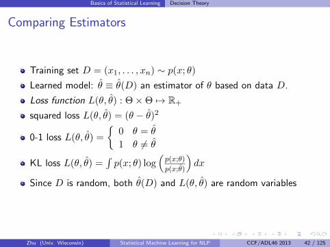
Training set D = (x1, . . . , xn) ∼ p(x; θ)
Learned model: θ ≡ θ(D) an estimator of θ based on data D.
Loss function L(θ, θ) : Θ×Θ 7→ R+
squared loss L(θ, θ) = (θ − θ)2
0-1 loss L(θ, θ) =
0 θ = θ
1 θ 6= θ
KL loss L(θ, θ) =∫p(x; θ) log
(p(x;θ)
p(x;θ)
)dx
Since D is random, both θ(D) and L(θ, θ) are random variables
Zhu (Univ. Wisconsin) Statistical Machine Learning for NLP CCF/ADL46 2013 42 / 125

Basics of Statistical Learning Decision Theory
Risk
The risk R(θ, θ) is the expected loss
R(θ, θ) = ED[L(θ, θ(D))]
ED averaged over training sets D sampled from the true θ
The risk is the “average training set” behavior of a learning algorithmwhen the world is θ
Not computable: we don’t know which θ the world is in.
Example: Let D = X1 ∼ N(θ, 1). Let θ1 = X1 and θ2 = 3.14.Assume squared loss. Then R(θ, θ1) = 1 (hint: variance),R(θ, θ2) = ED(θ − 3.14)2 = (θ − 3.14)2.
Smart learning algorithm θ1 and a dumb one θ2. However, for tasksθ ∈ (3.14− 1, 3.14 + 1) the dumb algorithm is better.
Zhu (Univ. Wisconsin) Statistical Machine Learning for NLP CCF/ADL46 2013 43 / 125

Basics of Statistical Learning Decision Theory
Minimax Estimator
maximum riskRmax(θ) = sup
θR(θ, θ)
The minimax estimator θminimax minimizes the maximum risk
θminimax = arg infθ
supθR(θ, θ)
The infimum is over all estimators θ.
The minimax estimator is the “best” in guarding against the worstpossible world.
Zhu (Univ. Wisconsin) Statistical Machine Learning for NLP CCF/ADL46 2013 44 / 125

Graphical Models
Outline
1 Basics of Statistical LearningProbabilityStatistical EstimationRegularizationDecision Theory
2 Graphical ModelsDirected Graphical Models (Bayesian Networks)Undirected Graphical Models (Markov Random Fields)Factor GraphMarkov Chain Monte CarloBelief PropagationMean Field AlgorithmMaximizing Problems (Viterbi)
3 Bayesian Non-Parametric ModelsDirichlet Processes
Zhu (Univ. Wisconsin) Statistical Machine Learning for NLP CCF/ADL46 2013 45 / 125

Graphical Models
The envelope quiz
Random variables E ∈ 1, 0, B ∈ r, bP (E = 1) = P (E = 0) = 1/2
P (B = r | E = 1) = 1/2, P (B = r | E = 0) = 0
We ask: P (E = 1 | B = b) ≥ 1/2?
P (E = 1 | B = b) = P (B=b|E=1)P (E=1)P (B=b) = 1/2×1/2
3/4 = 1/3
Switch.
The graphical model:
B
E
Zhu (Univ. Wisconsin) Statistical Machine Learning for NLP CCF/ADL46 2013 46 / 125

Graphical Models
Probabilistic Reasoning
The world is reduced to a set of random variables x1, . . . , xnI e.g. (x1, . . . , xn−1) a feature vector, xn ≡ y the class label
Inference: given joint distribution p(x1, . . . , xn), computep(XQ | XE) where XQ ∪XE ⊆ x1 . . . xn
I e.g. Q = n, E = 1 . . . n− 1, by the definition of conditional
p(xn | x1, . . . , xn−1) =p(x1, . . . , xn−1, xn)∑
v p(x1, . . . , xn−1, xn = v)
Learning: estimate p(x1, . . . , xn) from training data X(1), . . . , X(N),
where X(i) = (x(i)1 , . . . , x
(i)n )
Zhu (Univ. Wisconsin) Statistical Machine Learning for NLP CCF/ADL46 2013 47 / 125
Graphical Models
It is difficult to reason with uncertainty
joint distribution p(x1, . . . , xn)I exponential naıve storage (2n for binary r.v.)I hard to interpret (conditional independence)
inference p(XQ | XE)I Often can’t afford to do it by brute force
If p(x1, . . . , xn) not given, estimate it from dataI Often can’t afford to do it by brute force
Zhu (Univ. Wisconsin) Statistical Machine Learning for NLP CCF/ADL46 2013 48 / 125

Graphical Models
Graphical models
Graphical models: efficient representation, inference, and learning onp(x1, . . . , xn), exactly or approximately
Two main “flavors”:I directed graphical models = Bayesian Networks (often frequentist
instead of Bayesian)I undirected graphical models = Markov Random Fields
Key idea: make conditional independence explicit
Zhu (Univ. Wisconsin) Statistical Machine Learning for NLP CCF/ADL46 2013 49 / 125
Graphical Models Directed Graphical Models (Bayesian Networks)
Outline
1 Basics of Statistical LearningProbabilityStatistical EstimationRegularizationDecision Theory
2 Graphical ModelsDirected Graphical Models (Bayesian Networks)Undirected Graphical Models (Markov Random Fields)Factor GraphMarkov Chain Monte CarloBelief PropagationMean Field AlgorithmMaximizing Problems (Viterbi)
3 Bayesian Non-Parametric ModelsDirichlet Processes
Zhu (Univ. Wisconsin) Statistical Machine Learning for NLP CCF/ADL46 2013 50 / 125

Graphical Models Directed Graphical Models (Bayesian Networks)
Bayesian Network
Directed graphical models are also called Bayesian networks
A directed graph has nodes X = (x1, . . . , xn), some of themconnected by directed edges xi → xj
A cycle is a directed path x1 → . . .→ xk where x1 = xk
A directed acyclic graph (DAG) contains no cycles
A Bayesian network on the DAG is a family of distributions satisfying
p | p(X) =∏i
p(xi | Pa(xi))
where Pa(xi) is the set of parents of xi.
p(xi | Pa(xi)) is the conditional probability distribution (CPD) at xi
By specifying the CPDs for all i, we specify a particular distributionp(X)
Zhu (Univ. Wisconsin) Statistical Machine Learning for NLP CCF/ADL46 2013 51 / 125

Graphical Models Directed Graphical Models (Bayesian Networks)
Example: Alarm
Binary variables
P(A | B, E) = 0.95P(A | B, ~E) = 0.94P(A | ~B, E) = 0.29P(A | ~B, ~E) = 0.001
P(J | A) = 0.9P(J | ~A) = 0.05
P(M | A) = 0.7P(M | ~A) = 0.01
A
J M
B E
P(E)=0.002P(B)=0.001
P (B,∼ E,A, J,∼M)
= P (B)P (∼ E)P (A | B,∼ E)P (J | A)P (∼M | A)
= 0.001× (1− 0.002)× 0.94× 0.9× (1− 0.7)
≈ .000253
Zhu (Univ. Wisconsin) Statistical Machine Learning for NLP CCF/ADL46 2013 52 / 125

Graphical Models Directed Graphical Models (Bayesian Networks)
Example: Naive Bayes
y y
x x. . .1 d x
d
p(y, x1, . . . xd) = p(y)∏di=1 p(xi | y)
Used extensively in natural language processing
Plate representation on the right
Zhu (Univ. Wisconsin) Statistical Machine Learning for NLP CCF/ADL46 2013 53 / 125

Graphical Models Directed Graphical Models (Bayesian Networks)
No Causality Whatsoever
P(A)=aP(B|A)=bP(B|~A)=c
A
B
B
A
P(B)=ab+(1−a)cP(A|B)=ab/(ab+(1−a)c)P(A|~B)=a(1−b)/(1−ab−(1−a)c)
The two BNs are equivalent in all respects
Bayesian networks imply no causality at all
They only encode the joint probability distribution (hence correlation)
However, people tend to design BNs based on causal relations
Zhu (Univ. Wisconsin) Statistical Machine Learning for NLP CCF/ADL46 2013 54 / 125

Graphical Models Directed Graphical Models (Bayesian Networks)
Example: Latent Dirichlet Allocation (LDA)
θ
Ndw
D
αβT
zφ
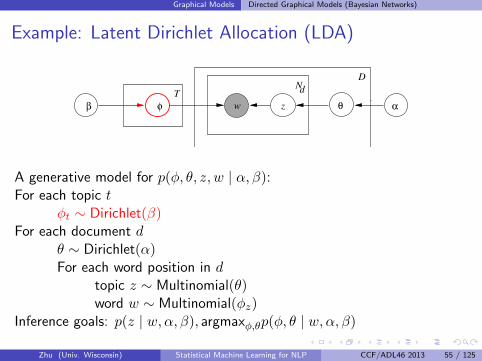
A generative model for p(φ, θ, z, w | α, β):For each topic t
φt ∼ Dirichlet(β)For each document d
θ ∼ Dirichlet(α)For each word position in d
topic z ∼ Multinomial(θ)word w ∼ Multinomial(φz)
Inference goals: p(z | w,α, β), argmaxφ,θp(φ, θ | w,α, β)
Zhu (Univ. Wisconsin) Statistical Machine Learning for NLP CCF/ADL46 2013 55 / 125

Graphical Models Directed Graphical Models (Bayesian Networks)
Example: Latent Dirichlet Allocation (LDA)
θ
Ndw
D
αβT
zφ
A generative model for p(φ, θ, z, w | α, β):For each topic t
φt ∼ Dirichlet(β)For each document d
θ ∼ Dirichlet(α)For each word position in d
topic z ∼ Multinomial(θ)word w ∼ Multinomial(φz)
Inference goals: p(z | w,α, β), argmaxφ,θp(φ, θ | w,α, β)
Zhu (Univ. Wisconsin) Statistical Machine Learning for NLP CCF/ADL46 2013 55 / 125

Graphical Models Directed Graphical Models (Bayesian Networks)
Example: Latent Dirichlet Allocation (LDA)
Ndw
D
αβT
zφ θ
A generative model for p(φ, θ, z, w | α, β):For each topic t
φt ∼ Dirichlet(β)For each document d
θ ∼ Dirichlet(α)For each word position in d
topic z ∼ Multinomial(θ)word w ∼ Multinomial(φz)
Inference goals: p(z | w,α, β), argmaxφ,θp(φ, θ | w,α, β)
Zhu (Univ. Wisconsin) Statistical Machine Learning for NLP CCF/ADL46 2013 55 / 125

Graphical Models Directed Graphical Models (Bayesian Networks)
Example: Latent Dirichlet Allocation (LDA)
θ
Ndw
D
αβT
zφ
A generative model for p(φ, θ, z, w | α, β):For each topic t
φt ∼ Dirichlet(β)For each document d
θ ∼ Dirichlet(α)For each word position in d
topic z ∼ Multinomial(θ)word w ∼ Multinomial(φz)
Inference goals: p(z | w,α, β), argmaxφ,θp(φ, θ | w,α, β)
Zhu (Univ. Wisconsin) Statistical Machine Learning for NLP CCF/ADL46 2013 55 / 125

Graphical Models Directed Graphical Models (Bayesian Networks)
Example: Latent Dirichlet Allocation (LDA)
θ
Ndw
D
αβT
zφ
A generative model for p(φ, θ, z, w | α, β):For each topic t
φt ∼ Dirichlet(β)For each document d
θ ∼ Dirichlet(α)For each word position in d
topic z ∼ Multinomial(θ)word w ∼ Multinomial(φz)
Inference goals: p(z | w,α, β), argmaxφ,θp(φ, θ | w,α, β)
Zhu (Univ. Wisconsin) Statistical Machine Learning for NLP CCF/ADL46 2013 55 / 125

Graphical Models Directed Graphical Models (Bayesian Networks)
Some Topics by LDA on the Wish Corpus
p(word | topic)
“troops” “election” “love”
Zhu (Univ. Wisconsin) Statistical Machine Learning for NLP CCF/ADL46 2013 56 / 125

Graphical Models Directed Graphical Models (Bayesian Networks)
Conditional Independence
Two r.v.s A, B are independent if P (A,B) = P (A)P (B) orP (A|B) = P (A) (the two are equivalent)
Two r.v.s A, B are conditionally independent given C ifP (A,B | C) = P (A | C)P (B | C) or P (A | B,C) = P (A | C) (thetwo are equivalent)
This extends to groups of r.v.s
Conditional independence in a BN is precisely specified byd-separation (“directed separation”)
Zhu (Univ. Wisconsin) Statistical Machine Learning for NLP CCF/ADL46 2013 57 / 125

Graphical Models Directed Graphical Models (Bayesian Networks)
d-Separation Case 1: Tail-to-Tail
C
A B
C
A B
A, B in general dependent
A, B conditionally independent given C (observed nodes are shaded)
An observed C is a tail-to-tail node, blocks the undirected path A-B
Zhu (Univ. Wisconsin) Statistical Machine Learning for NLP CCF/ADL46 2013 58 / 125

Graphical Models Directed Graphical Models (Bayesian Networks)
d-Separation Case 2: Head-to-Tail
A C B A C B
A, B in general dependent
A, B conditionally independent given C
An observed C is a head-to-tail node, blocks the path A-B
Zhu (Univ. Wisconsin) Statistical Machine Learning for NLP CCF/ADL46 2013 59 / 125

Graphical Models Directed Graphical Models (Bayesian Networks)
d-Separation Case 3: Head-to-Head
A B A B
C C
A, B in general independent
A, B conditionally dependent given C, or any of C’s descendants
An observed C is a head-to-head node, unblocks the path A-B
Zhu (Univ. Wisconsin) Statistical Machine Learning for NLP CCF/ADL46 2013 60 / 125
Graphical Models Directed Graphical Models (Bayesian Networks)
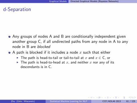
d-Separation
Any groups of nodes A and B are conditionally independent givenanother group C, if all undirected paths from any node in A to anynode in B are blocked
A path is blocked if it includes a node x such that eitherI The path is head-to-tail or tail-to-tail at x and x ∈ C, orI The path is head-to-head at x, and neither x nor any of its
descendants is in C.
Zhu (Univ. Wisconsin) Statistical Machine Learning for NLP CCF/ADL46 2013 61 / 125

Graphical Models Directed Graphical Models (Bayesian Networks)
d-Separation Example 1
The undirected path from A to B is unblocked by E (because of C),and is not blocked by F
A, B dependent given C
A
C
B
F
E
Zhu (Univ. Wisconsin) Statistical Machine Learning for NLP CCF/ADL46 2013 62 / 125
Graphical Models Directed Graphical Models (Bayesian Networks)
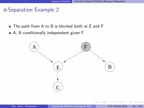
d-Separation Example 2
The path from A to B is blocked both at E and F
A, B conditionally independent given F
A
B
F
E
C
Zhu (Univ. Wisconsin) Statistical Machine Learning for NLP CCF/ADL46 2013 63 / 125

Graphical Models Undirected Graphical Models (Markov Random Fields)
Outline
1 Basics of Statistical LearningProbabilityStatistical EstimationRegularizationDecision Theory
2 Graphical ModelsDirected Graphical Models (Bayesian Networks)Undirected Graphical Models (Markov Random Fields)Factor GraphMarkov Chain Monte CarloBelief PropagationMean Field AlgorithmMaximizing Problems (Viterbi)
3 Bayesian Non-Parametric ModelsDirichlet Processes
Zhu (Univ. Wisconsin) Statistical Machine Learning for NLP CCF/ADL46 2013 64 / 125

Graphical Models Undirected Graphical Models (Markov Random Fields)
Markov Random Fields
Undirected graphical models are also called Markov Random Fields
The efficiency of directed graphical model (acyclic graph, locallynormalized CPDs) also makes it restrictive
A clique C in an undirected graph is a fully connected set of nodes(note: full of loops!)
Define a nonnegative potential function ψC : XC 7→ R+
An undirected graphical model is a family of distributions satisfyingp | p(X) =
1
Z
∏C
ψC(XC)
Z =∫ ∏
C ψC(XC)dX is the partition function
Zhu (Univ. Wisconsin) Statistical Machine Learning for NLP CCF/ADL46 2013 65 / 125

Graphical Models Undirected Graphical Models (Markov Random Fields)
Example: A Tiny Markov Random Field
x x1 2
C
x1, x2 ∈ −1, 1A single clique ψC(x1, x2) = eax1x2
p(x1, x2) = 1Z e
ax1x2
Z = (ea + e−a + e−a + ea)
p(1, 1) = p(−1,−1) = ea/(2ea + 2e−a)
p(−1, 1) = p(1,−1) = e−a/(2ea + 2e−a)
When the parameter a > 0, favor homogeneous chains
When the parameter a < 0, favor inhomogeneous chains
Zhu (Univ. Wisconsin) Statistical Machine Learning for NLP CCF/ADL46 2013 66 / 125

Graphical Models Undirected Graphical Models (Markov Random Fields)
Log Linear Models
Real-valued feature functions f1(X), . . . , fk(X)
Real-valued weights w1, . . . , wk
p(X) =1
Zexp
(−
k∑i=1
wifi(X)
)
Zhu (Univ. Wisconsin) Statistical Machine Learning for NLP CCF/ADL46 2013 67 / 125
Graphical Models Undirected Graphical Models (Markov Random Fields)
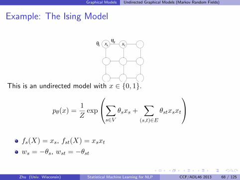
Example: The Ising Model
θsθ
xs xtst
This is an undirected model with x ∈ 0, 1.
pθ(x) =1
Zexp
∑s∈V
θsxs +∑
(s,t)∈E
θstxsxt
fs(X) = xs, fst(X) = xsxt
ws = −θs, wst = −θst
Zhu (Univ. Wisconsin) Statistical Machine Learning for NLP CCF/ADL46 2013 68 / 125

Graphical Models Undirected Graphical Models (Markov Random Fields)
Example: Image Denoising
[From Bishop PRML] noisy image argmaxXP (X|Y )
pθ(X | Y ) =1
Zexp
∑s∈V
θsxs +∑
(s,t)∈E
θstxsxt
θs =
c ys = 1−c ys = 0
Zhu (Univ. Wisconsin) Statistical Machine Learning for NLP CCF/ADL46 2013 69 / 125

Graphical Models Undirected Graphical Models (Markov Random Fields)
Example: Gaussian Random Field
p(X) ∼ N(µ,Σ) =1
(2π)n/2|Σ|1/2exp
(−1
2(X − µ)>Σ−1(X − µ)
)
Multivariate Gaussian
The n× n covariance matrix Σ positive semi-definite
Let Ω = Σ−1 be the precision matrix
xi, xj are conditionally independent given all other variables, if andonly if Ωij = 0
When Ωij 6= 0, there is an edge between xi, xj
Zhu (Univ. Wisconsin) Statistical Machine Learning for NLP CCF/ADL46 2013 70 / 125

Graphical Models Undirected Graphical Models (Markov Random Fields)
Conditional Independence in Markov Random Fields
Two group of variables A, B are conditionally independent givenanother group C, if:
A, B become disconnected by removing C and all edges involving C
AC
B
Zhu (Univ. Wisconsin) Statistical Machine Learning for NLP CCF/ADL46 2013 71 / 125

Graphical Models Factor Graph
Outline
1 Basics of Statistical LearningProbabilityStatistical EstimationRegularizationDecision Theory
2 Graphical ModelsDirected Graphical Models (Bayesian Networks)Undirected Graphical Models (Markov Random Fields)Factor GraphMarkov Chain Monte CarloBelief PropagationMean Field AlgorithmMaximizing Problems (Viterbi)
3 Bayesian Non-Parametric ModelsDirichlet Processes
Zhu (Univ. Wisconsin) Statistical Machine Learning for NLP CCF/ADL46 2013 72 / 125

Graphical Models Factor Graph
Factor Graph
For both directed and undirected graphical models
Bipartite: edges between a variable node and a factor node
Factors represent computation
A B
C
(A,B,C)ψ
A B
C
A B
C
(A,B,C)ψf
A B
C
fP(A)P(B)P(C|A,B)
Zhu (Univ. Wisconsin) Statistical Machine Learning for NLP CCF/ADL46 2013 73 / 125

Graphical Models Markov Chain Monte Carlo
Outline
1 Basics of Statistical LearningProbabilityStatistical EstimationRegularizationDecision Theory
2 Graphical ModelsDirected Graphical Models (Bayesian Networks)Undirected Graphical Models (Markov Random Fields)Factor GraphMarkov Chain Monte CarloBelief PropagationMean Field AlgorithmMaximizing Problems (Viterbi)
3 Bayesian Non-Parametric ModelsDirichlet Processes
Zhu (Univ. Wisconsin) Statistical Machine Learning for NLP CCF/ADL46 2013 74 / 125

Graphical Models Markov Chain Monte Carlo
Inference by Monte Carlo
Consider the inference problem p(XQ = cQ | XE) whereXQ ∪XE ⊆ x1 . . . xn
p(XQ = cQ | XE) =
∫1(xQ=cQ)p(xQ | XE)dxQ
If we can draw samples x(1)Q , . . . x
(m)Q ∼ p(xQ | XE), an unbiased
estimator is
p(XQ = cQ | XE) ≈ 1
m
m∑i=1
1(x
(i)Q =cQ)
The variance of the estimator decreases as O(1/m)
Inference reduces to sampling from p(xQ | XE)
We discuss two methods: forward sampling and Gibbs sampling
Zhu (Univ. Wisconsin) Statistical Machine Learning for NLP CCF/ADL46 2013 75 / 125

Graphical Models Markov Chain Monte Carlo
Forward Sampling: Example
P(A | B, E) = 0.95P(A | B, ~E) = 0.94P(A | ~B, E) = 0.29P(A | ~B, ~E) = 0.001
P(J | A) = 0.9P(J | ~A) = 0.05
P(M | A) = 0.7P(M | ~A) = 0.01
A
J M
B E
P(E)=0.002P(B)=0.001
To generate a sample X = (B,E,A, J,M):
1 Sample B ∼ Ber(0.001): r ∼ U(0, 1). If (r < 0.001) then B = 1 elseB = 0
2 Sample E ∼ Ber(0.002)
3 If B = 1 and E = 1, sample A ∼ Ber(0.95), and so on
4 If A = 1 sample J ∼ Ber(0.9) else J ∼ Ber(0.05)
5 If A = 1 sample M ∼ Ber(0.7) else M ∼ Ber(0.01)
Zhu (Univ. Wisconsin) Statistical Machine Learning for NLP CCF/ADL46 2013 76 / 125

Graphical Models Markov Chain Monte Carlo
Inference with Forward Sampling
Say the inference task is P (B = 1 | E = 1,M = 1)
Throw away all samples except those with (E = 1,M = 1)
p(B = 1 | E = 1,M = 1) ≈ 1
m
m∑i=1
1(B(i)=1)
where m is the number of surviving samples
Can be highly inefficient (note P (E = 1) tiny)
Does not work for Markov Random Fields
Zhu (Univ. Wisconsin) Statistical Machine Learning for NLP CCF/ADL46 2013 77 / 125

Graphical Models Markov Chain Monte Carlo
Gibbs Sampler: Example P (B = 1 | E = 1,M = 1)
Gibbs sampler is a Markov Chain Monte Carlo (MCMC) method.
Directly sample from p(xQ | XE)
Works for both graphical models
Initialization:I Fix evidence; randomly set other variablesI e.g. X(0) = (B = 0, E = 1, A = 0, J = 0,M = 1)
P(A | B, E) = 0.95P(A | B, ~E) = 0.94P(A | ~B, E) = 0.29P(A | ~B, ~E) = 0.001
P(J | A) = 0.9P(J | ~A) = 0.05
P(M | A) = 0.7P(M | ~A) = 0.01
A
J
B
P(E)=0.002P(B)=0.001
E=1
M=1
Zhu (Univ. Wisconsin) Statistical Machine Learning for NLP CCF/ADL46 2013 78 / 125

Graphical Models Markov Chain Monte Carlo
Gibbs UpdateFor each non-evidence variable xi, fixing all other nodes X−i,resample its value xi ∼ P (xi | X−i)This is equivalent to xi ∼ P (xi | MarkovBlanket(xi))For a Bayesian network MarkovBlanket(xi) includes xi’s parents,spouses, and children
P (xi | MarkovBlanket(xi)) ∝ P (xi | Pa(xi))∏
y∈C(xi)
P (y | Pa(y))
where Pa(x) are the parents of x, and C(x) the children of x.For many graphical models the Markov Blanket is small.For example, B ∼ P (B | E = 1, A = 0) ∝ P (B)P (A = 0 | B,E = 1)
P(A | B, E) = 0.95P(A | B, ~E) = 0.94P(A | ~B, E) = 0.29P(A | ~B, ~E) = 0.001
P(J | A) = 0.9P(J | ~A) = 0.05
P(M | A) = 0.7P(M | ~A) = 0.01
A
J
B
P(E)=0.002P(B)=0.001
E=1
M=1
Zhu (Univ. Wisconsin) Statistical Machine Learning for NLP CCF/ADL46 2013 79 / 125

Graphical Models Markov Chain Monte Carlo
Gibbs Update
Say we sampled B = 1. ThenX(1) = (B = 1, E = 1, A = 0, J = 0,M = 1)
Starting from X(1), sample A ∼ P (A | B = 1, E = 1, J = 0,M = 1)to get X(2)
Move on to J , then repeat B,A, J,B,A, J . . .
Keep all later samples. P (B = 1 | E = 1,M = 1) is the fraction ofsamples with B = 1.
P(A | B, E) = 0.95P(A | B, ~E) = 0.94P(A | ~B, E) = 0.29P(A | ~B, ~E) = 0.001
P(J | A) = 0.9P(J | ~A) = 0.05
P(M | A) = 0.7P(M | ~A) = 0.01
A
J
B
P(E)=0.002P(B)=0.001
E=1
M=1
Zhu (Univ. Wisconsin) Statistical Machine Learning for NLP CCF/ADL46 2013 80 / 125
Graphical Models Markov Chain Monte Carlo
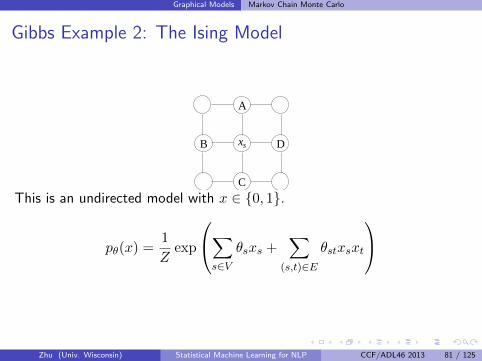
Gibbs Example 2: The Ising Model
xs
A
B
C
D
This is an undirected model with x ∈ 0, 1.
pθ(x) =1
Zexp
∑s∈V
θsxs +∑
(s,t)∈E
θstxsxt
Zhu (Univ. Wisconsin) Statistical Machine Learning for NLP CCF/ADL46 2013 81 / 125

Graphical Models Markov Chain Monte Carlo
Gibbs Example 2: The Ising Model
xs
A
B
C
D
The Markov blanket of xs is A,B,C,D
In general for undirected graphical models
p(xs | x−s) = p(xs | xN(s))
N(s) is the neighbors of s.
The Gibbs update is
p(xs = 1 | xN(s)) =1
exp(−(θs +∑
t∈N(s) θstxt)) + 1
Zhu (Univ. Wisconsin) Statistical Machine Learning for NLP CCF/ADL46 2013 82 / 125

Graphical Models Markov Chain Monte Carlo
Gibbs Sampling as a Markov Chain
A Markov chain is defined by a transition matrix T (X ′ | X)
Certain Markov chains have a stationary distribution π such thatπ = Tπ
Gibbs sampler is such a Markov chain withTi((X−i, x
′i) | (X−i, xi)) = p(x′i | X−i), and stationary distribution
p(xQ | XE)
But it takes time for the chain to reach stationary distribution (mix)I Can be difficult to assert mixingI In practice “burn in”: discard X(0), . . . , X(T )
I Use all of X(T+1), . . . for inference (they are correlated); Do not thin
Zhu (Univ. Wisconsin) Statistical Machine Learning for NLP CCF/ADL46 2013 83 / 125

Graphical Models Markov Chain Monte Carlo
Collapsed Gibbs Sampling
In general, Ep[f(X)] ≈ 1m
∑mi=1 f(X(i)) if X(i) ∼ p
Sometimes X = (Y,Z) where Z has closed-form operations
If so,
Ep[f(X)] = Ep(Y )Ep(Z|Y )[f(Y,Z)]
≈ 1
m
m∑i=1
Ep(Z|Y (i))[f(Y (i), Z)]
if Y (i) ∼ p(Y )
No need to sample Z: it is collapsed
Collapsed Gibbs sampler Ti((Y−i, y′i) | (Y−i, yi)) = p(y′i | Y−i)
Note p(y′i | Y−i) =∫p(y′i, Z | Y−i)dZ
Zhu (Univ. Wisconsin) Statistical Machine Learning for NLP CCF/ADL46 2013 84 / 125

Graphical Models Markov Chain Monte Carlo
Example: Collapsed Gibbs Sampling for LDA
θ
Ndw
D
αβT
zφ
Collapse θ, φ, Gibbs update:
P (zi = j | z−i,w) ∝n
(wi)−i,j + βn
(di)−i,j + α
n(·)−i,j +Wβn
(di)−i,· + Tα
n(wi)−i,j : number of times word wi has been assigned to topic j,
excluding the current position
n(di)−i,j : number of times a word from document di has been assigned
to topic j, excluding the current position
n(·)−i,j : number of times any word has been assigned to topic j,
excluding the current position
n(di)−i,·: length of document di, excluding the current position
Zhu (Univ. Wisconsin) Statistical Machine Learning for NLP CCF/ADL46 2013 85 / 125

Graphical Models Markov Chain Monte Carlo
Summary: Markov Chain Monte Carlo
Forward sampling
Gibbs sampling
Collapsed Gibbs sampling
Not covered: block Gibbs, Metropolis-Hastings, etc.
Unbiased (after burn-in), but can have high variance
Zhu (Univ. Wisconsin) Statistical Machine Learning for NLP CCF/ADL46 2013 86 / 125

Graphical Models Belief Propagation
Outline
1 Basics of Statistical LearningProbabilityStatistical EstimationRegularizationDecision Theory
2 Graphical ModelsDirected Graphical Models (Bayesian Networks)Undirected Graphical Models (Markov Random Fields)Factor GraphMarkov Chain Monte CarloBelief PropagationMean Field AlgorithmMaximizing Problems (Viterbi)
3 Bayesian Non-Parametric ModelsDirichlet Processes
Zhu (Univ. Wisconsin) Statistical Machine Learning for NLP CCF/ADL46 2013 87 / 125

Graphical Models Belief Propagation
The Sum-Product Algorithm
Also known as belief propagation (BP)
Exact if the graph is a tree; otherwise known as “loopy BP”,approximate
The algorithm involves passing messages on the factor graph
Alternative view: variational approximation (more later)
Zhu (Univ. Wisconsin) Statistical Machine Learning for NLP CCF/ADL46 2013 88 / 125

Graphical Models Belief Propagation
Example: A Simple HMM
The Hidden Markov Model template (not a graphical model)
π = π = 1/21 2
P(x | z=1)=(1/2, 1/4, 1/4) P(x | z=2)=(1/4, 1/2, 1/4)
1 2
1/4 1/2
R G B R G B
Zhu (Univ. Wisconsin) Statistical Machine Learning for NLP CCF/ADL46 2013 89 / 125

Graphical Models Belief Propagation
Example: A Simple HMM
Observing x1 = R, x2 = G, the directed graphical model
z1
x =G2
z2
x =R1
Factor graphz1f 1 z2f 2
P(z )P(x | z ) P(z | z )P(x | z )1 1 1 2 1 2 2
Zhu (Univ. Wisconsin) Statistical Machine Learning for NLP CCF/ADL46 2013 90 / 125

Graphical Models Belief Propagation
Messages
A message is a vector of length K, where K is the number of valuesx takes.
There are two types of messages:1 µf→x: message from a factor node f to a variable node xµf→x(i) is the ith element, i = 1 . . .K.
2 µx→f : message from a variable node x to a factor node f
Zhu (Univ. Wisconsin) Statistical Machine Learning for NLP CCF/ADL46 2013 91 / 125

Graphical Models Belief Propagation
Leaf Messages
Assume tree factor graph. Pick an arbitrary root, say z2
Start messages at leaves.
If a leaf is a factor node f , µf→x(x) = f(x)
µf1→z1(z1 = 1) = P (z1 = 1)P (R|z1 = 1) = 1/2 · 1/2 = 1/4
µf1→z1(z1 = 2) = P (z1 = 2)P (R|z1 = 2) = 1/2 · 1/4 = 1/8
If a leaf is a variable node x, µx→f (x) = 1
z1f 1 z2f 2
P(z )P(x | z ) P(z | z )P(x | z )1 1 1 2 1 2 2
π = π = 1/21 2
P(x | z=1)=(1/2, 1/4, 1/4) P(x | z=2)=(1/4, 1/2, 1/4)
1 2
1/4 1/2
R G B R G B
Zhu (Univ. Wisconsin) Statistical Machine Learning for NLP CCF/ADL46 2013 92 / 125
Graphical Models Belief Propagation
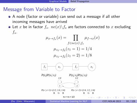
Message from Variable to FactorA node (factor or variable) can send out a message if all otherincoming messages have arrivedLet x be in factor fs. ne(x)\fs are factors connected to x excludingfs.
µx→fs(x) =∏
f∈ne(x)\fs
µf→x(x)
µz1→f2(z1 = 1) = 1/4
µz1→f2(z1 = 2) = 1/8
z1f 1 z2f 2
P(z )P(x | z ) P(z | z )P(x | z )1 1 1 2 1 2 2
π = π = 1/21 2
P(x | z=1)=(1/2, 1/4, 1/4) P(x | z=2)=(1/4, 1/2, 1/4)
1 2
1/4 1/2
R G B R G B
Zhu (Univ. Wisconsin) Statistical Machine Learning for NLP CCF/ADL46 2013 93 / 125

Graphical Models Belief Propagation
Message from Factor to Variable
Let x be in factor fs. Let the other variables in fs be x1:M .
µfs→x(x) =∑x1
. . .∑xM
fs(x, x1, . . . , xM )
M∏m=1
µxm→fs(xm)
In this example
µf2→z2(s) =
2∑s′=1
µz1→f2(s′)f2(z1 = s′, z2 = s)
= 1/4P (z2 = s|z1 = 1)P (x2 = G|z2 = s)
+1/8P (z2 = s|z1 = 2)P (x2 = G|z2 = s)
We get µf2→z2(z2 = 1) = 1/32, µf2→z2(z2 = 2) = 1/8
z1f 1 z2f 2
P(z )P(x | z ) P(z | z )P(x | z )1 1 1 2 1 2 2
Zhu (Univ. Wisconsin) Statistical Machine Learning for NLP CCF/ADL46 2013 94 / 125

Graphical Models Belief Propagation
Up to Root, Back Down
The message has reached the root, pass it back down
µz2→f2(z2 = 1) = 1
µz2→f2(z2 = 2) = 1
z1f 1 z2f 2
P(z )P(x | z ) P(z | z )P(x | z )1 1 1 2 1 2 2
π = π = 1/21 2
P(x | z=1)=(1/2, 1/4, 1/4) P(x | z=2)=(1/4, 1/2, 1/4)
1 2
1/4 1/2
R G B R G B
Zhu (Univ. Wisconsin) Statistical Machine Learning for NLP CCF/ADL46 2013 95 / 125

Graphical Models Belief Propagation
Keep Passing Down
µf2→z1(s) =∑2
s′=1 µz2→f2(s′)f2(z1 = s, z2 = s′)= 1P (z2 = 1|z1 = s)P (x2 = G|z2 = 1)
+ 1P (z2 = 2|z1 = s)P (x2 = G|z2 = 2).
We getµf2→z1(z1 = 1) = 7/16µf2→z1(z1 = 2) = 3/8
z1f 1 z2f 2
P(z )P(x | z ) P(z | z )P(x | z )1 1 1 2 1 2 2
π = π = 1/21 2
P(x | z=1)=(1/2, 1/4, 1/4) P(x | z=2)=(1/4, 1/2, 1/4)
1 2
1/4 1/2
R G B R G B
Zhu (Univ. Wisconsin) Statistical Machine Learning for NLP CCF/ADL46 2013 96 / 125

Graphical Models Belief Propagation
From Messages to Marginals
Once a variable receives all incoming messages, we compute itsmarginal as
p(x) ∝∏
f∈ne(x)
µf→x(x)
In this example
P (z1|x1, x2) ∝ µf1→z1 · µf2→z1 =( 1/4
1/8
)·( 7/16
3/8
)=( 7/64
3/64
)⇒(
0.70.3
)P (z2|x1, x2) ∝ µf2→z2 =
( 1/321/8
)⇒(
0.20.8
)One can also compute the marginal of the set of variables xs involvedin a factor fs
p(xs) ∝ fs(xs)∏
x∈ne(f)
µx→f (x)
Zhu (Univ. Wisconsin) Statistical Machine Learning for NLP CCF/ADL46 2013 97 / 125

Graphical Models Belief Propagation
Handling Evidence
Observing x = v,I we can absorb it in the factor (as we did); orI set messages µx→f (x) = 0 for all x 6= v
Observing XE ,I multiplying the incoming messages to x /∈ XE gives the joint (notp(x|XE)):
p(x,XE) ∝∏
f∈ne(x)
µf→x(x)
I The conditional is easily obtained by normalization
p(x|XE) =p(x,XE)∑x′ p(x′, XE)
Zhu (Univ. Wisconsin) Statistical Machine Learning for NLP CCF/ADL46 2013 98 / 125

Graphical Models Belief Propagation
Loopy Belief Propagation
So far, we assumed a tree graph
When the factor graph contains loops, pass messages indefinitely untilconvergence
But convergence may not happen
But in many cases loopy BP still works well, empirically
Zhu (Univ. Wisconsin) Statistical Machine Learning for NLP CCF/ADL46 2013 99 / 125

Graphical Models Mean Field Algorithm
Outline
1 Basics of Statistical LearningProbabilityStatistical EstimationRegularizationDecision Theory
2 Graphical ModelsDirected Graphical Models (Bayesian Networks)Undirected Graphical Models (Markov Random Fields)Factor GraphMarkov Chain Monte CarloBelief PropagationMean Field AlgorithmMaximizing Problems (Viterbi)
3 Bayesian Non-Parametric ModelsDirichlet Processes
Zhu (Univ. Wisconsin) Statistical Machine Learning for NLP CCF/ADL46 2013 100 / 125

Graphical Models Mean Field Algorithm
Example: The Ising Model
θsθ
xs xtst
The random variables x take values in 0, 1.
pθ(x) =1
Zexp
∑s∈V
θsxs +∑
(s,t)∈E
θstxsxt
Zhu (Univ. Wisconsin) Statistical Machine Learning for NLP CCF/ADL46 2013 101 / 125

Graphical Models Mean Field Algorithm
The Conditional
θsθ
xs xtst
Markovian: the conditional distribution for xs is
p(xs | x−s) = p(xs | xN(s))
N(s) is the neighbors of s.
This reduces to (recall Gibbs sampling)
p(xs = 1 | xN(s)) =1
exp(−(θs +∑
t∈N(s) θstxt)) + 1
Zhu (Univ. Wisconsin) Statistical Machine Learning for NLP CCF/ADL46 2013 102 / 125
Graphical Models Mean Field Algorithm
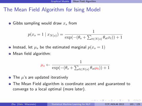
The Mean Field Algorithm for Ising Model
Gibbs sampling would draw xs from
p(xs = 1 | xN(s)) =1
exp(−(θs +∑
t∈N(s) θstxt)) + 1
Instead, let µs be the estimated marginal p(xs = 1)
Mean field algorithm:
µs ←1
exp(−(θs +∑
t∈N(s) θstµt)) + 1
The µ’s are updated iteratively
The Mean Field algorithm is coordinate ascent and guaranteed toconverge to a local optimal (more later).
Zhu (Univ. Wisconsin) Statistical Machine Learning for NLP CCF/ADL46 2013 103 / 125

Graphical Models Maximizing Problems (Viterbi)
Outline
1 Basics of Statistical LearningProbabilityStatistical EstimationRegularizationDecision Theory
2 Graphical ModelsDirected Graphical Models (Bayesian Networks)Undirected Graphical Models (Markov Random Fields)Factor GraphMarkov Chain Monte CarloBelief PropagationMean Field AlgorithmMaximizing Problems (Viterbi)
3 Bayesian Non-Parametric ModelsDirichlet Processes
Zhu (Univ. Wisconsin) Statistical Machine Learning for NLP CCF/ADL46 2013 104 / 125

Graphical Models Maximizing Problems (Viterbi)
Maximizing ProblemsRecall the HMM example
π = π = 1/21 2
P(x | z=1)=(1/2, 1/4, 1/4) P(x | z=2)=(1/4, 1/2, 1/4)
1 2
1/4 1/2
R G B R G B
There are two senses of “best states” z1:N given x1:N :1 So far we computed the marginal p(zn|x1:N )
I We can define “best” as z∗n = arg maxk p(zn = k|x1:N )I However z∗1:N as a whole may not be the bestI In fact z∗1:N can even have zero probability!
2 An alternative is to find
z∗1:N = arg maxz1:N
p(z1:N |x1:N )
I finds the most likely state configuration as a wholeI The max-sum algorithm solves this, generalizes the Viterbi algorithm
for HMMsZhu (Univ. Wisconsin) Statistical Machine Learning for NLP CCF/ADL46 2013 105 / 125

Graphical Models Maximizing Problems (Viterbi)
Intermediate: The Max-Product Algorithm
Simple modification to the sum-product algorithm: replace∑
with max inthe factor-to-variable messages.
µfs→x(x) = maxx1
. . .maxxM
fs(x, x1, . . . , xM )
M∏m=1
µxm→fs(xm)
µxm→fs(xm) =∏
f∈ne(xm)\fs
µf→xm(xm)
µxleaf→f(x) = 1
µfleaf→x(x) = f(x)
Zhu (Univ. Wisconsin) Statistical Machine Learning for NLP CCF/ADL46 2013 106 / 125

Graphical Models Maximizing Problems (Viterbi)
Intermediate: The Max-Product Algorithm
As in sum-product, pick an arbitrary variable node x as the root
Pass messages up from leaves until they reach the root
Unlike sum-product, do not pass messages back from root to leaves
At the root, multiply incoming messages
pmax = maxx
∏f∈ne(x)
µf→x(x)
This is the probability of the most likely state configuration
Zhu (Univ. Wisconsin) Statistical Machine Learning for NLP CCF/ADL46 2013 107 / 125

Graphical Models Maximizing Problems (Viterbi)
Intermediate: The Max-Product Algorithm
To identify the configuration itself, keep back pointers:
When creating the message
µfs→x(x) = maxx1
. . .maxxM
fs(x, x1, . . . , xM )
M∏m=1
µxm→fs(xm)
for each x value, we separately create M pointers back to the valuesof x1, . . . , xM that achieve the maximum.
At the root, backtrack the pointers.
Zhu (Univ. Wisconsin) Statistical Machine Learning for NLP CCF/ADL46 2013 108 / 125

Graphical Models Maximizing Problems (Viterbi)
Intermediate: The Max-Product Algorithm
z1f 1 z2f 2
P(z )P(x | z ) P(z | z )P(x | z )1 1 1 2 1 2 2
π = π = 1/21 2
P(x | z=1)=(1/2, 1/4, 1/4) P(x | z=2)=(1/4, 1/2, 1/4)
1 2
1/4 1/2
R G B R G B
Message from leaf f1
µf1→z1(z1 = 1) = P (z1 = 1)P (R|z1 = 1) = 1/2 · 1/2 = 1/4µf1→z1(z1 = 2) = P (z1 = 2)P (R|z1 = 2) = 1/2 · 1/4 = 1/8
The second messageµz1→f2(z1 = 1) = 1/4µz1→f2(z1 = 2) = 1/8
Zhu (Univ. Wisconsin) Statistical Machine Learning for NLP CCF/ADL46 2013 109 / 125

Graphical Models Maximizing Problems (Viterbi)
Intermediate: The Max-Product Algorithm
z1f 1 z2f 2
P(z )P(x | z ) P(z | z )P(x | z )1 1 1 2 1 2 2
π = π = 1/21 2
P(x | z=1)=(1/2, 1/4, 1/4) P(x | z=2)=(1/4, 1/2, 1/4)
1 2
1/4 1/2
R G B R G B
µf2→z2(z2 = 1)
= maxz1
f2(z1, z2)µz1→f2(z1)
= maxz1
P (z2 = 1 | z1)P (x2 = G | z2 = 1)µz1→f2(z1)
= max(1/4 · 1/4 · 1/4, 1/2 · 1/4 · 1/8) = 1/64
Back pointer for z2 = 1: either z1 = 1 or z1 = 2
Zhu (Univ. Wisconsin) Statistical Machine Learning for NLP CCF/ADL46 2013 110 / 125

Graphical Models Maximizing Problems (Viterbi)
Intermediate: The Max-Product Algorithm
z1f 1 z2f 2
P(z )P(x | z ) P(z | z )P(x | z )1 1 1 2 1 2 2
π = π = 1/21 2
P(x | z=1)=(1/2, 1/4, 1/4) P(x | z=2)=(1/4, 1/2, 1/4)
1 2
1/4 1/2
R G B R G B
The other element of the same message:
µf2→z2(z2 = 2)
= maxz1
f2(z1, z2)µz1→f2(z1)
= maxz1
P (z2 = 2 | z1)P (x2 = G | z2 = 2)µz1→f2(z1)
= max(3/4 · 1/2 · 1/4, 1/2 · 1/2 · 1/8) = 3/32
Back pointer for z2 = 2: z1 = 1
Zhu (Univ. Wisconsin) Statistical Machine Learning for NLP CCF/ADL46 2013 111 / 125
Graphical Models Maximizing Problems (Viterbi)
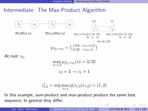
Intermediate: The Max-Product Algorithm
z1f 1 z2f 2
P(z )P(x | z ) P(z | z )P(x | z )1 1 1 2 1 2 2
π = π = 1/21 2
P(x | z=1)=(1/2, 1/4, 1/4) P(x | z=2)=(1/4, 1/2, 1/4)
1 2
1/4 1/2
R G B R G B
µf2→z2 =( 1/64 →z1=1,2
3/32 →z1=1
)At root z2,
maxs=1,2
µf2→z2(s) = 3/32
z2 = 2→ z1 = 1
z∗1:2 = arg maxz1:2
p(z1:2|x1:2) = (1, 2)
In this example, sum-product and max-product produce the same bestsequence; In general they differ.
Zhu (Univ. Wisconsin) Statistical Machine Learning for NLP CCF/ADL46 2013 112 / 125

Graphical Models Maximizing Problems (Viterbi)
From Max-Product to Max-SumThe max-sum algorithm is equivalent to the max-product algorithm, butwork in log space to avoid underflow.
µfs→x(x) = maxx1...xM
log fs(x, x1, . . . , xM ) +
M∑m=1
µxm→fs(xm)
µxm→fs(xm) =∑
f∈ne(xm)\fs
µf→xm(xm)
µxleaf→f(x) = 0
µfleaf→x(x) = log f(x)
When at the root,
log pmax = maxx
∑f∈ne(x)
µf→x(x)
The back pointers are the same.
Zhu (Univ. Wisconsin) Statistical Machine Learning for NLP CCF/ADL46 2013 113 / 125

Bayesian Non-Parametric Models
Outline
1 Basics of Statistical LearningProbabilityStatistical EstimationRegularizationDecision Theory
2 Graphical ModelsDirected Graphical Models (Bayesian Networks)Undirected Graphical Models (Markov Random Fields)Factor GraphMarkov Chain Monte CarloBelief PropagationMean Field AlgorithmMaximizing Problems (Viterbi)
3 Bayesian Non-Parametric ModelsDirichlet Processes
Zhu (Univ. Wisconsin) Statistical Machine Learning for NLP CCF/ADL46 2013 114 / 125

Bayesian Non-Parametric Models
Stochastic Process
Infinite collection of random variables indexed by a set x.x ∈ R for “time”
More generally, x ∈ Rd (e.g., space and time).
Zhu (Univ. Wisconsin) Statistical Machine Learning for NLP CCF/ADL46 2013 115 / 125

Bayesian Non-Parametric Models Dirichlet Processes
Outline
1 Basics of Statistical LearningProbabilityStatistical EstimationRegularizationDecision Theory
2 Graphical ModelsDirected Graphical Models (Bayesian Networks)Undirected Graphical Models (Markov Random Fields)Factor GraphMarkov Chain Monte CarloBelief PropagationMean Field AlgorithmMaximizing Problems (Viterbi)
3 Bayesian Non-Parametric ModelsDirichlet Processes
Zhu (Univ. Wisconsin) Statistical Machine Learning for NLP CCF/ADL46 2013 116 / 125

Bayesian Non-Parametric Models Dirichlet Processes
Base Distribution
Let H be a base distribution over a probability space Θ.
Example: Θ = Rd.
An element θ ∈ Rd is an index to the stochastic process
H = N(0,Σ) is a base distribution over Θ, but not a stochasticprocess.
H(θ) = N(θ; 0,Σ) is not a random variable (it is a fixed value for agiven θ)
Zhu (Univ. Wisconsin) Statistical Machine Learning for NLP CCF/ADL46 2013 117 / 125

Bayesian Non-Parametric Models Dirichlet Processes
Stick-Breaking Construction of Dirichlet Process
βk ∼ Beta(1, α)
πk = βk
k−1∏i=1
(1− βi)
θ∗k ∼ H
G =
∞∑k=1
πkδθ∗k
δz is the point mass function on z
π1, π2, . . . are stick fragments which tend to (but not always) getsmaller. Sum to 1.
Each fragment is associated with an index θ∗k sampled from the basedistribution H
G is a sample from a Dirichlet Process G ∼ DP (α,H)
Zhu (Univ. Wisconsin) Statistical Machine Learning for NLP CCF/ADL46 2013 118 / 125

Bayesian Non-Parametric Models Dirichlet Processes
Properties of G
G is a probability measure on Θ (naturally normalized), similar to thebase distribution H.
With probability one, G is a discrete measure (true even if H is acontinuous measure, e.g. Gaussian).
θ’s drawn from G have repeats. Useful to model clusters.
Zhu (Univ. Wisconsin) Statistical Machine Learning for NLP CCF/ADL46 2013 119 / 125

Bayesian Non-Parametric Models Dirichlet Processes
More Properties of Dirichlet Process
G ∼ DP (α,H)
Marginals of G are Dirichlet-distributed: Let A1, . . . , Ar be any finitemeasurable partition of Θ, then
(G(A1), . . . , G(Ar)) ∼ Dirichlet(αH(A1), . . . , αH(Ar))
For any measurable A ⊆ Θ,
E[G(A)] = H(A) V[G(A)] =H(A)(1−H(A))
1 + α
As α→∞, G(A)→ H(A) for any measurable A.
Zhu (Univ. Wisconsin) Statistical Machine Learning for NLP CCF/ADL46 2013 120 / 125
Bayesian Non-Parametric Models Dirichlet Processes
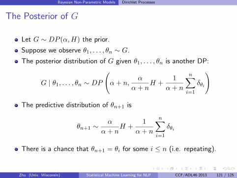
The Posterior of G
Let G ∼ DP (α,H) the prior.
Suppose we observe θ1, . . . , θn ∼ G.
The posterior distribution of G given θ1, . . . , θn is another DP:
G | θ1, . . . , θn ∼ DP
(α+ n,
α
α+ nH +
1
α+ n
n∑i=1
δθi
)
The predictive distribution of θn+1 is
θn+1 ∼α
α+ nH +
1
α+ n
n∑i=1
δθi
There is a chance that θn+1 = θi for some i ≤ n (i.e. repeating).
Zhu (Univ. Wisconsin) Statistical Machine Learning for NLP CCF/ADL46 2013 121 / 125

Bayesian Non-Parametric Models Dirichlet Processes
The Blackwell-MacQueen Urn Scheme
Assume samples from H do not repeat (e.g. Gaussian)
Let θ∗1 . . . θ∗m be the unique values in θ1 . . . θn
Let nk =∑n
i=1 1θi=θ∗k for k = 1 . . .m.
θn+1 is generated with the following procedure:1 With probability α/(α+ n), draw a new value from H and assign it toθn+1;
2 Otherwise, reuse value θ∗k with probability nk/n.3 We add θn+1 to the samples, and repeat this process.
Zhu (Univ. Wisconsin) Statistical Machine Learning for NLP CCF/ADL46 2013 122 / 125

Bayesian Non-Parametric Models Dirichlet Processes
The Chinese Restaurant Process
The equality relationship in θ1 . . . θn defines a partition of n items.
The first customer sits at the first table.
With probability α/(α+ n) the (n+ 1)-th customer sits at a newtable; otherwise he joins an existing table with probabilityproportional to the number of people already sitting there.
Chinese Restaurant Process (CRP) defines a distribution overpartitions of items.
CRP + (for a new table draw a dish θ ∼ H; all customers sitting onthis table eat the dish) = DP
Zhu (Univ. Wisconsin) Statistical Machine Learning for NLP CCF/ADL46 2013 123 / 125

Bayesian Non-Parametric Models Dirichlet Processes
Dirichlet Process Mixture Models (DPMMs)
Infinite mixture models: unlimited number of clusters
G ∼ DP (α,H)
θi ∼ G
xi ∼ F (θ)
where F (θ) is an appropriate distribution parametrized by θ (e.g.multinomial).
Each observation xi has its own parameter θi.
Many of the θi’s are identical, naturally inducing a clusteringstructure over x.
Given x1 . . .xn, α,H, F , use MCMC to infer θ1 . . . θn
Zhu (Univ. Wisconsin) Statistical Machine Learning for NLP CCF/ADL46 2013 124 / 125

Bayesian Non-Parametric Models Dirichlet Processes
References
Bishop, Pattern Recognition and Machine Learning. Springer 2006.
Hastie, Tibshirani, Friedman. The Elements of Statistical Learning:Data Mining, Inference, and Prediction. Second Edition, 2009.
Koller & Friedman, Probabilistic Graphical Models. MIT 2009.
Murphy, Machine Learning: a Probabilistic Perspective, 2012.
Wasserman, All of Statistics: A Concise Course in StatisticalInference. Springer 2003.
Zhu (Univ. Wisconsin) Statistical Machine Learning for NLP CCF/ADL46 2013 125 / 125