statistical performance provisioning and energy …
TRANSCRIPT

STATISTICAL PERFORMANCE
PROVISIONING AND ENERGY EFFICIENCY
IN DISTRIBUTED COMPUTING SYSTEMS
Nikzad Babaii Rizvandi
Supervisors: Prof.Albert Y.Zomaya
Prof. Aruna Seneviratne 1

OUTLINE
Introduction
Background
Our research direction
Part 1 - Energy efficiency in Hardware using DVFS
Background
Multiple frequencies selection algorithm
Observations and mathematical proofs
Part 2 - Statistical performance provisioning for jobs
on MapReduce framework
Background
Statistical pattern matching for finding similarity between
MapReduce applications grouping/ classification
Statistical learning for performance analysis and
provisioning of MapReduce jobs modeling
2

World data centres used*
1% of the total world electricity consumption in 2005
equivalent to about seventeen 1000MW power plants
growth of around 76% in five years period (2000-2005,
2005-2010)
Improper usage of 44 million servers in the world **
Produce 11.8 million tons of carbon dioxide
Equivalent of 2.1 million cars
INTRODUCTION
* Koomey, J.G. ,”Worldwide electricity used in data centres”, Environ.Res. Lett. , 2008
** Alliance to Save Energy (ASE) and 1E, "Server Energy and Efficiency Report," 2009 3
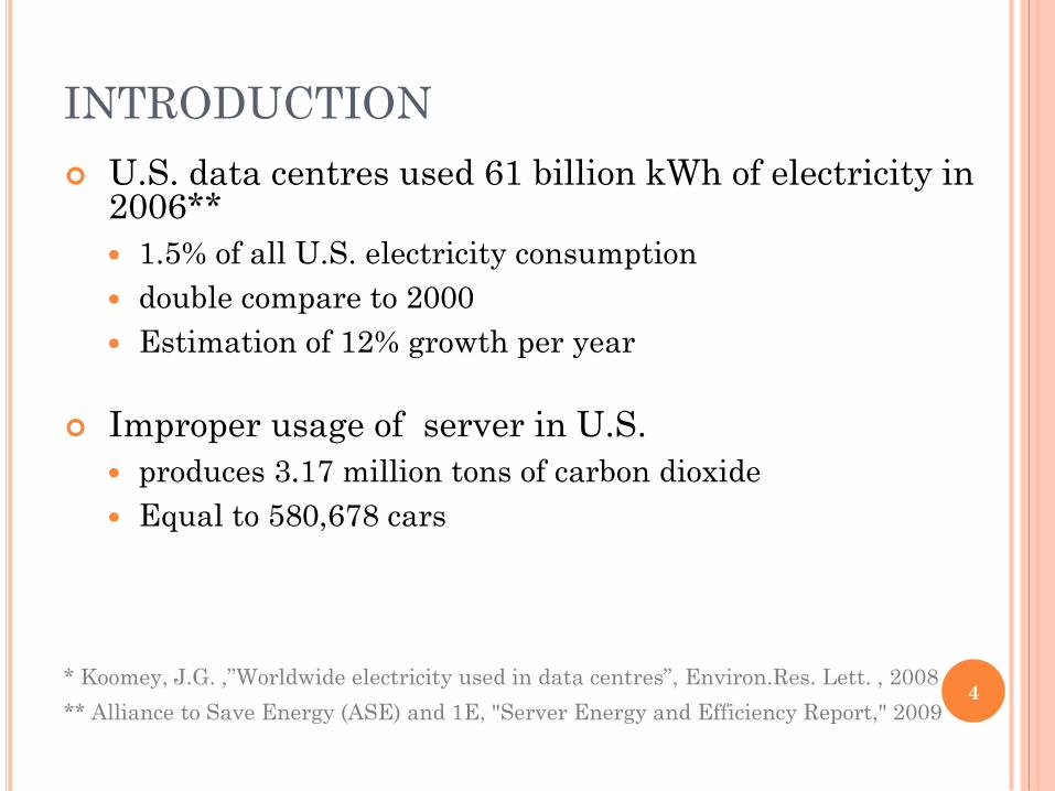
U.S. data centres used 61 billion kWh of electricity in 2006**
1.5% of all U.S. electricity consumption
double compare to 2000
Estimation of 12% growth per year
Improper usage of server in U.S.
produces 3.17 million tons of carbon dioxide
Equal to 580,678 cars
INTRODUCTION
* Koomey, J.G. ,”Worldwide electricity used in data centres”, Environ.Res. Lett. , 2008
** Alliance to Save Energy (ASE) and 1E, "Server Energy and Efficiency Report," 2009
4

ENERGY CONSUMPTION IN DISTRIBUTED
SYSTEMS
5
6
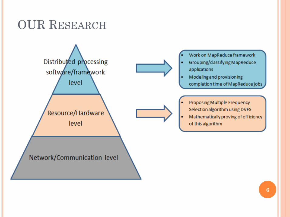
OUR RESEARCH

PART 1 - ENERGY EFFICIENCY IN
DISTRIBUTED COMPUTING SYSTEMS USING
DVFS
7

In CMOS circuits: 𝐸 = 𝑘𝑓𝑣2𝑡
𝑓 ∝ 𝑣⇒ 𝐸 ∝ 𝑓3𝑡
Example:
𝑓 ⟶ 𝑓′ =𝑓
2⇒
𝑡′ = 2𝑡
𝐸′ = 𝑘(𝑓′)2𝑡′ = 𝑘 𝑓3
82𝑡 =
𝐸
4
BACKGROUND – Dynamic Voltage
Frequency Scaling
8

BACKGROUND – Dynamic Voltage
Frequency Scaling
Each task has a maximum time restriction.
In hypothetical world
processors has continuous frequency.
For 𝑘𝑡ℎ task, Optimum Continuous Frequency (𝑓𝑜𝑝𝑡𝑖𝑚𝑢𝑚(𝑘)
)
is a frequency that uses the maximum time restriction of
the task. 9

BACKGROUND – Dynamic Voltage
Frequency Scaling
In reality
processors has a discrete set of frequencies
𝑓1 > ⋯ > 𝑓𝑁 .
The best frequency is slightly over 𝑓𝑜𝑝𝑡𝑖𝑚𝑢𝑚(𝑘)
.
10
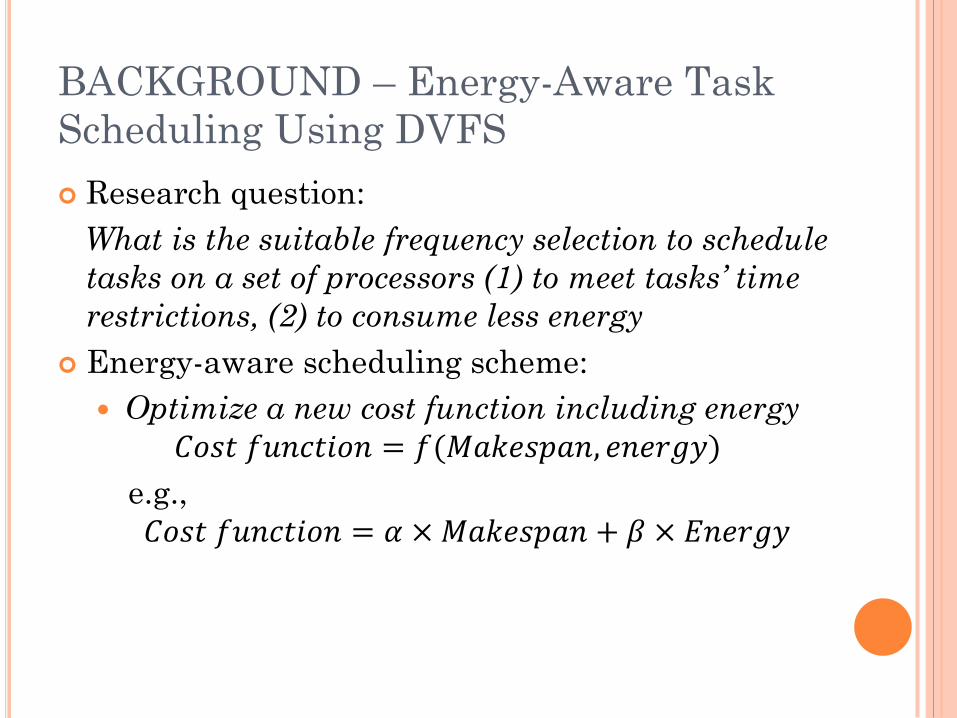
Research question:
What is the suitable frequency selection to schedule
tasks on a set of processors (1) to meet tasks’ time
restrictions, (2) to consume less energy
Energy-aware scheduling scheme:
Optimize a new cost function including energy
𝐶𝑜𝑠𝑡 𝑓𝑢𝑛𝑐𝑡𝑖𝑜𝑛 = 𝑓(𝑀𝑎𝑘𝑒𝑠𝑝𝑎𝑛, 𝑒𝑛𝑒𝑟𝑔𝑦)
e.g.,
𝐶𝑜𝑠𝑡 𝑓𝑢𝑛𝑐𝑡𝑖𝑜𝑛 = 𝛼 ×𝑀𝑎𝑘𝑒𝑠𝑝𝑎𝑛 + 𝛽 × 𝐸𝑛𝑒𝑟𝑔𝑦
BACKGROUND – Energy-Aware Task
Scheduling Using DVFS
11

Slack reclamation
On top of scheduled tasks
Any slack on processors is used to reduce the speed of running
task
BACKGROUND – Energy-Aware Task
Scheduling Using DVFS
12

OUR WORK – Multiple Frequency Selection
(MFS-DVFS) for Slack Reclamation
Current scheme: use one frequency for a task (RDVFS
algorithm)
Our idea: use linear combination of all processor’s
frequencies for each task.
13
OUR WORK - Optimization Problem in
MFS-DVFS
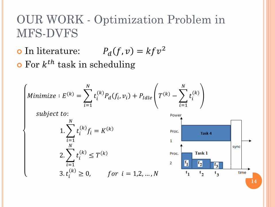
In literature: 𝑃𝑑 𝑓, 𝑣 = 𝑘𝑓𝑣2
For 𝑘𝑡ℎ task in scheduling
𝑀𝑖𝑛𝑖𝑚𝑖𝑧𝑒 ∶ 𝐸(𝑘) = 𝑡𝑖(𝑘)
𝑃𝑑 𝑓𝑖 , 𝑣𝑖 + 𝑃𝐼𝑑𝑙𝑒 𝑇(𝑘) − 𝑡𝑖(𝑘)
𝑁
𝑖=1
𝑁
𝑖=1
𝑠𝑢𝑏𝑗𝑒𝑐𝑡 𝑡𝑜:
1. 𝑡𝑖𝑘𝑓𝑖
𝑁
𝑖=1
= 𝐾 𝑘
2. 𝑡𝑖𝑘
≤ 𝑇 𝑘
𝑁
𝑖=1
3. 𝑡𝑖𝑘
≥ 0, 𝑓𝑜𝑟 𝑖 = 1,2, … , 𝑁
14

MFS-DVFS – Algorithm
Input: the scheduled tasks on a set of P processors
1. For 𝑘𝑡ℎ task (𝐴(𝑘)) scheduled on processor 𝑃𝑗
2. Solve optimization problem by linear programming
3. end for
4. return (the voltages and frequencies of optimal
execution of the task)
15

In literature: 𝑃𝑑 𝑓, 𝑣 = 𝑘𝑓𝑣2
Generalization: 𝑃𝑑 𝑓, 𝑣
If 𝑓𝑖 , 𝑣𝑖 < 𝑓𝑗 , 𝑣𝑗 then 𝑃𝑑 𝑓𝑖 , 𝑣𝑖 < 𝑃𝑑 𝑓𝑗 , 𝑣𝑗
Observation #1
In hypothetical world, the cont. frequency that uses
maximum time restriction of 𝑘𝑡ℎ task gives the
optimum energy saving (𝑓𝑜𝑝𝑡𝑖𝑚𝑢𝑚(𝑘)
)
Observation #2
For 𝑘𝑡ℎ task, always up to two voltage-frequencies
are involved in optimal energy consumption (𝑓𝑖 < 𝑓𝑗)
Proof: theorem 1, 2
OBSERVATION – Mathematical Proofs*
* N.B.Rizvandi, et al., “Some observations on optimal frequency selection in DVFS-
based energy consumption minimization”, J. Parallel Distrib. Comput. 71(8): 1154-
1164 (2011)
16

Observation #3
𝑓𝑖 < 𝑓𝑜𝑝𝑡𝑖𝑚𝑢𝑚(𝑘)
< 𝑓𝑗
Proof: lemma 1, 2
Observation #4
The associated time for these frequencies (𝑡𝑖 , 𝑡𝑗) is
𝑡𝑖(𝑘)
=𝐾(𝑘)−𝑇(𝑘)𝑓𝑖
𝑓𝑗−𝑓𝑖
𝑡𝑗(𝑘)
=𝑇(𝑘)𝑓𝑗−𝐾
(𝑘)
𝑓𝑗−𝑓𝑖
Proof: Corollary 1
OBSERVATION – Mathematical Proofs*
* N.B.Rizvandi, et al., “Some observations on optimal frequency selection in DVFS-
based energy consumption minimization”, J. Parallel Distrib. Comput. 71(8): 1154-
1164 (2011)
17

Observation #5
The consumed energy of processor for this task
associated with these two voltage-frequencies is
𝐸(𝑘) =𝑇 𝑘 𝑓𝑗−𝐾
𝑘
𝑓𝑗−𝑓𝑖𝑃𝑑 𝑓𝑖 , 𝑣𝑖 +
𝐾(𝑘)−𝑇(𝑘)𝑓𝑖
𝑓𝑗−𝑓𝑖𝑃𝑑 𝑓𝑗 , 𝑣𝑗
Proof: Corollary 2
Observation #6
Using less time to execute the task results in more
energy consumption
Proof: theorem 3
OBSERVATION – Mathematical Proofs*
* N.B.Rizvandi, et al., “Some observations on optimal frequency selection in DVFS-
based energy consumption minimization”, J. Parallel Distrib. Comput. 71(8): 1154-
1164 (2011)
18

In a simplified version, 𝑓 ∝ 𝑣 then 𝑃𝑑 𝑓, 𝑣 = 𝜆𝑓3
Observation #7
These two frequencies are neighbors. i.e., two
immediate frequencies around 𝑓𝑜𝑝𝑡𝑖𝑚𝑢𝑚(𝑘)
Proof: theorem 4, 5
OBSERVATION – Mathematical Proofs*
* N.B.Rizvandi, et al., “Some observations on optimal frequency selection in DVFS-
based energy consumption minimization”, J. Parallel Distrib. Comput. 71(8): 1154-
1164 (2011)
19

MFS-DVFS – New Algorithm
Input: the scheduled tasks on a set of P processors
1. For 𝑘𝑡ℎ task (𝐴(𝑘)) scheduled on processor 𝑃𝑗
2. Calculate 𝑓𝑜𝑝𝑡𝑖𝑚𝑢𝑚(𝑘)
3. Select the neighbour frequencies in the
processor’s frequency set before and after
𝑓𝑜𝑝𝑡𝑖𝑚𝑢𝑚(𝑘)
. These frequencies are 𝑓𝑅𝐷(𝑘)
and 𝑓𝑅𝐷−1(𝑘)
.
4. Calculate associated times and energy consumption.
5. Select 𝑓𝑅𝐷(𝑘)
, 𝑓𝑅𝐷−1(𝑘)
associated to the lowest
energy for this task
6. end for
return (individual frequencies pair for execution of each
task)
20

Simulation settings
Scheduler
List scheduler
List scheduler with Longest Processing Time First (LPT)
List scheduler with Shortest Processing Time First (SPT)
Processor power model *
Transmeta Crusoe
Intel Xscale
Two synthetic processors
EXPERIMENTAL RESULTS - Simulator
21

Task graphs (DAG)
Random
LU-decomposition
Gauss-Jordan
Assumption: switching time between frequencies can be ignored
compare to task execution time
Experimental parameters
EXPERIMENTAL RESULTS - Simulator
Parameter Value
# of tasks 100, 200, 300, 400, 500
# of processors 2, 4, 8, 16, 32
22
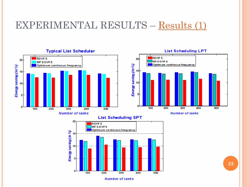
EXPERIMENTAL RESULTS – Results (1)
23

EXPERIMENTAL RESULTS – Results (2)
24
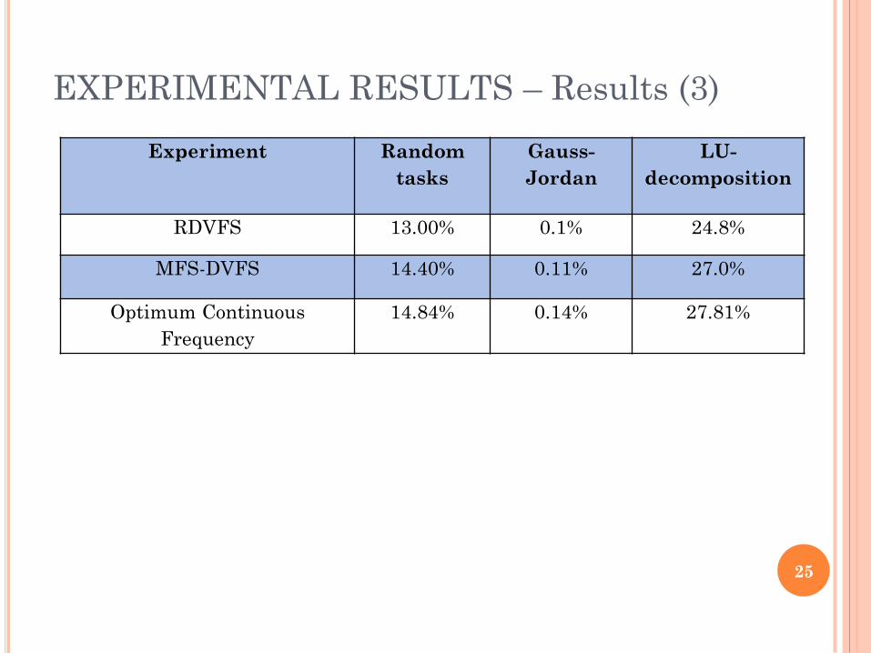
Experiment Random
tasks
Gauss-
Jordan
LU-
decomposition
RDVFS 13.00% 0.1% 24.8%
MFS-DVFS 14.40% 0.11% 27.0%
Optimum Continuous
Frequency
14.84% 0.14% 27.81%
EXPERIMENTAL RESULTS – Results (3)
25

PART 2 – PERFORMANCE ANALYSIS AND
PROVISIONING IN MAPREDUCE CLUSTERS
26

A parametric distributed processing framework for
processing large data sets.
Introduced by Google in 2004.
Typically used for distributed computing on clusters
of computers.
Widely used in Google, Yahoo, Facebook and
LinkedIn.
Hadoop is famous open source version of
MapReduce developed by Apache
BACKGROUND – MapReduce
27

Many users have job completion time goals
There is strong correlation between completion time and values of configuration parameters
No support from current service providers, e.g. Amazon Elastic MapReduce
Sole responsibility of user to set values for these parameters.
Our research work
Calculate similarity between MapReduce applications. It is too likely similar applications show similar performance for the same values of configuration parameters.
Estimate a function to model the dependency between completion time and configuration parameters by using Machine Learning techniques on historical data.
MOTIVATION
28

Classification
Two MapReduce applications belong to the same group if
they have similar CPU utilization pattern for several
identical jobs.
An identical job in two applications means they run with
the same values for configuration parameters
the same size of small input data.
hypothesis
Similar Applications share the same optimal values for
the configuration parameters.
obtain the optimal values of configuration parameters for one
application and use for others in the same group.
CLASSIFICATION
29
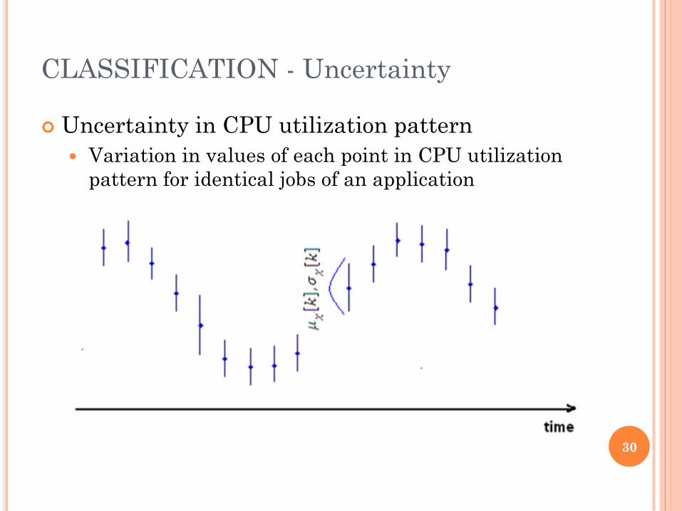
Uncertainty in CPU utilization pattern
Variation in values of each point in CPU utilization
pattern for identical jobs of an application
CLASSIFICATION - Uncertainty
30

High similarity is equal to low distance
Current scheme
Average values of each point in patterns
Apply Dynamic Time Warping (DTW) on average CPU
patterns patterns become the same length
Calculate Euclidean distance between two average
patterns (i.e., 𝜑𝑎𝑣𝑟. and 𝜒𝑎𝑣𝑟.)
(𝜑𝑎𝑣𝑟. 𝑖 − 𝜒𝑎𝑣𝑟. [𝑖])2
𝑁
𝑖=1
≤ 𝑟
𝑟 predefined distance threshold
CLASSIFICATION – Similarity (1)
31

Our idea*
Comes from computational finance background.
Each point in the pattern has a Gaussian distribution.
After DTW between two patterns 𝜑𝑢 , 𝜒𝑢, use uncertain
Euclidean distance as
P 𝐷𝑆𝑇 𝜑𝑢 , 𝜒𝑢 = (𝜑𝑢 𝑖 − 𝜒𝑢 𝑖 )2𝑁
𝑖=1
≤ 𝑟 ≥ 𝜏
𝜑𝑢 𝑖 = ℕ(𝑚𝑒𝑎𝑛(𝜑𝑢 𝑖 )𝜑𝑐 𝑖
, 𝑣𝑎𝑟(𝜑𝑢 𝑖 ))𝑒𝜑
𝑗
𝜒𝑢 𝑗 = ℕ(𝑚𝑒𝑎𝑛(𝜒𝑢[𝑗])𝜒𝑐[𝑗]
+ 𝑣𝑎𝑟(𝜒𝑢[𝑗])𝑒𝜒
𝑗
)
0 < 𝜏 ≤ 1 is predefined probability threshold
CLASSIFICATION – Similarity (2)
* N.B.Rizvandi, et al., “A Study on Using Uncertain Time Series Matching Algorithms
in Map-Reduce Applications”, Concurrency and Computation: Practice and Experience,
2012
32

Calculate 𝑟𝑏𝑜𝑢𝑛𝑑𝑟𝑦 as
𝑟𝑏𝑜𝑢𝑛𝑑𝑟𝑦 =𝑟𝑏𝑜𝑢𝑛𝑑𝑟𝑦,𝑛𝑜𝑟𝑚2 − 𝐸(𝐷2[𝑖])𝑁
𝑖=1
𝑉𝑎𝑟 𝐷2 𝑖𝑁𝑖=1
𝑟𝑏𝑜𝑢𝑛𝑑𝑟𝑦,𝑛𝑜𝑟𝑚 = 2 × erf−1(2𝜏 − 1)
If choose r ≤ 𝑟𝑏𝑜𝑢𝑛𝑑𝑟𝑦, this guarantees that
P 𝐷𝑆𝑇 𝜑𝑢 , 𝜒𝑢 ≤ 𝑟𝑏𝑜𝑢𝑛𝑑𝑟𝑦 ≥ 𝜏
So, 𝑟𝑏𝑜𝑢𝑛𝑑𝑟𝑦 is the minimum distance between two
patterns with probability 𝜏
P 𝐷𝑆𝑇 𝜑𝑢 , 𝜒𝑢 = 𝑟𝑏𝑜𝑢𝑛𝑑𝑟𝑦 = 𝜏
CLASSIFICATION – Similarity (3)
* N.B.Rizvandi, et al., “A Study on Using Uncertain Time Series Matching Algorithms
in Map-Reduce Applications”, Concurrency and Computation: Practice and Experience,
2012
33

CLASSIFICATION – technique
* N.B.Rizvandi, et al., “A Study on Using Uncertain Time Series Matching Algorithms
in Map-Reduce Applications”, Concurrency and Computation: Practice and Experience,
2012
34
Hadoop cluster settings
Five servers, dual-core
Xen Cloud Platform (XCP)
Xen-API to measure performance statistics
10 Virtual machines
Application settings
Four legacy applications: WordCount, TeraSort, Exim
Mainlog parsing, Distributed Grep
Input data size
5GB, 10GB, 15GB, 20GB
# of map/reduce tasks
4, 8, 12, 16, 20, 24, 28, 32
Total number of runs in our experiments
8 × 8 × 5 × 4 × 10 × 4 = 51200
EXPERIMENTAL RESULTS – Setting
35
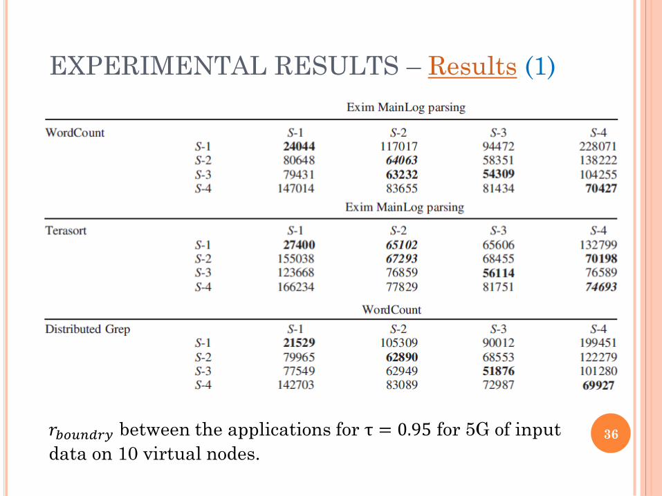
EXPERIMENTAL RESULTS – Results (1)
𝑟𝑏𝑜𝑢𝑛𝑑𝑟𝑦 between the applications for τ = 0.95 for 5G of input
data on 10 virtual nodes. 36

EXPERIMENTAL RESULTS – Results (2)
The size of input data vs. 𝑟𝑏𝑜𝑢𝑛𝑑𝑟𝑦 for 𝜏 = 0.95 for 5G, 10G,
15G and 20G of input data on 10 virtual nodes.
0
50000
100000
150000
200000
250000
5 10 15 20
WordCount vs Exim Mainlog parsing
Set-1 Set-2 Set-3 Set-4
Set-5 Set-6 Set-7 Set-8
0
50000
100000
150000
200000
250000
300000
5 10 15 20
Terasort vs. Exim Mainlog parsing
Set-1 Set-2 Set-3 Set-4
Set-5 Set-6 Set-7 Set-8
37
HOW TO USE THIS TECHNIQUE
For frequent running jobs (e.g., Indexing, Sorting,
Searching), run jobs with different values of conf.
parameters
For a new job, try to find most similar application
in DB (using this algorithm). Then use its optimal
values of parameters for running the new job.
38

Many users have job completion time goals
There is strong correlation between completion time and values of configuration parameters
No support from current service providers, e.g. Amazon Elastic MapReduce
Sole responsibility of user to set values for these parameters.
Our research work
Calculate similarity between MapReduce applications. It is too likely similar applications show similar performance for the same values of configuration parameters.
Estimate a function to model the dependency between completion time and configuration parameters by using Machine Learning techniques on historical data.
MOTIVATION
39

Profiling historical data
Run applications for different values of configuration
parameters (i.e., # of map tasks, # of reduce tasks, input
data size)
Profile completion time
Model selection (completion time vs. parameters)
polynomial regression has been widely used in
literature.
It estimates a global function which may not be accurate
enough at many points.
Suffers from over-fitting and under-fitting
Needs user observation of data to find the suitable polynomial
fit function
PERFORMANCE MODELLING AND
PROVISIONING – Our idea (1)
Cholesterol level (y-axis) vs. Age (x-axis)
40

We use a combination of K-NN and regression to
improve accuracy
K neighbours of a point are chosen.
A linear regression function is used to fit on data.
Generally higher accuracy than regression.
Can be chosen automatically.
PERFORMANCE MODELLING AND
PROVISIONING – Our idea (2)
Cholesterol level (y-axis) vs. Age (x-axis)
41

Prediction accuracy
Mean Absolute Percentage Error (MAPE)
𝑀𝐴𝑃𝐸 =
𝑡𝑒𝑥𝑐.
(𝑖) − 𝑡𝑒𝑥𝑐. (𝑖)
𝑡𝑒𝑥𝑐.(𝑖)
𝑀𝑖=1
𝑀
𝑅2 prediction accuracy
𝑅2 = 1 − (𝑡𝑒𝑥𝑐.
(𝑖) − 𝑡𝑒𝑥𝑐.(𝑖) )2𝑀
𝑖=1
(𝑡𝑒𝑥𝑐.(𝑖) −
𝑡𝑒𝑥𝑐.(𝑟)
𝑀𝑀𝑟=1 )2𝑀
𝑖=1
PERFORMANCE MODELLING AND
PROVISIONING – Our idea (3)
42

Hadoop cluster settings
Five servers, dual-core
SysStat to measure performance statistics
Hadoop 0.20.0
Application settings
Three applications: WordCount, TeraSort, Exim Mainlog
Input data size
3GB, 6GB, 8GB, 10GB
# of map/reduce tasks
80 number randomly chosen between 4 to 100
56 experiments for model estimation, rest for model testing
EXPERIMENTAL RESULTS – Setting
43
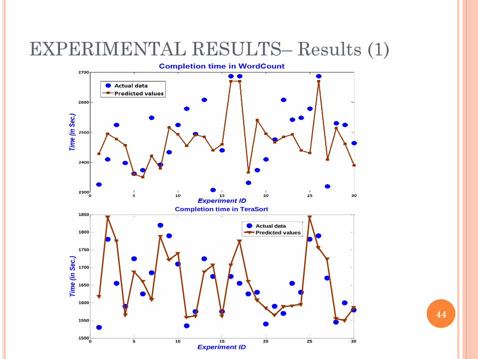
EXPERIMENTAL RESULTS– Results (1)
0 5 10 15 20 25 301500
1550
1600
1650
1700
1750
1800
1850
Experiment ID
Tim
e (
in S
ec.)
Completion time in TeraSort
Actual data
Predicted values
44

EXPERIMENTAL RESULTS– Results (3)
MAPE 𝑹𝟐 prediction accuracy
WordCount 1.51% 0.83
Exim MainLog
parsing
3.1% 0.76
TeraSort 2.33% 0.79
45
HOW TO USE THESE TECHNIQUES
For frequent running jobs (e.g., Indexing, Sorting,
Searching), run jobs with different values of conf.
parameters
Fit a model (based on second technique) and
calculate the optimal values of parameters which
minimizes completion time.
Put this application + optimal values into DB
For a new job, try to find most similar application
in DB (using first technique). Then use its optimal
values of parameters for running the new job.
Reducing completion time indirectly reduces
energy consumption.
46

References 1) Koomey, J.G. ,”Worldwide electricity used in data centres”, Environ.Res. Lett. ,
2008
2) Alliance to Save Energy (ASE) and 1E, "Server Energy and Efficiency Report,"
2009
3) Nikzad Babaii Rizvandi, et.al, "Multiple Frequency Selection in DVFS-Enabled
Processors to Minimize Energy Consumption," in Energy Efficient Distributed
Computing, 2011, John Wiley Publisher
4) Nikzad Babaii Rizvandi, et.al, “Some observations on Optimal Frequency Selection
in DVFS–based Energy Consumption Minimization in Clusters," Journal of
Parallel and Distributed Computing (JPDC), 2011.
5) Nikzad Babaii Rizvandi, et.al, "Linear Combinations of DVFS-enabled Processor
Frequencies to Modify the Energy-Aware Scheduling Algorithms," CCGrid 2010
6) Nikzad Babaii Rizvandi, et.al, “A Study on Using Uncertain Time Series Matching
Algorithms in Map-Reduce Applications”, Concurrency and Computation: Practice
and Experience, 2012
7) Nikzad Babaii Rizvandi, et.al, “Network Load Analysis and Provisioning for
MapReduce Applications”, PDCAT-2012
8) “Data-Intensive Workload Consolidation on Hadoop Distributed File System”,
Grid’12
9) Nikzad Babaii Rizvandi, et.al, "On Modelling and Prediction of Total CPU
Utilization for MapReduce Applications”, ICA3PP 2012
47