statistics and econometrics using xlispstat · 2009-05-28 · statistics and econometrics using...
TRANSCRIPT

STATISTICS AND ECONOMETRICSUSING XLISPSTAT
John E. FloydUniversity of Toronto
May 27, 2009

Contents
1 Introduction 1
2 Working with XLispStat 52.1 Using XLispStat as a Calculator . . . . . . . . . . . . . . . . 62.2 Defining Objects and Working with Lists . . . . . . . . . . . 82.3 Writing Lisp Functions . . . . . . . . . . . . . . . . . . . . . . 162.4 Working with Matrices . . . . . . . . . . . . . . . . . . . . . . 192.5 Reading and Writing Data Files . . . . . . . . . . . . . . . . . 262.6 Transforming Data . . . . . . . . . . . . . . . . . . . . . . . . 322.7 Error Messages . . . . . . . . . . . . . . . . . . . . . . . . . . 46
3 Descriptive Statistics 49
4 Hypothesis Tests 634.1 Probability Densities and Quantiles . . . . . . . . . . . . . . . 634.2 Plotting Probability Distributions . . . . . . . . . . . . . . . . 684.3 Generating Random Data . . . . . . . . . . . . . . . . . . . . 714.4 Tests of the Mean and Standard Deviation . . . . . . . . . . . 734.5 Tests of the Difference Between Two Means . . . . . . . . . . 754.6 Tests of Goodness of Fit . . . . . . . . . . . . . . . . . . . . . 80
5 Linear Regression Analysis 855.1 Using Matrix Calculations . . . . . . . . . . . . . . . . . . . . 865.2 Using the Regression-Model Function . . . . . . . . . . . . . . 905.3 Heteroskedasticity . . . . . . . . . . . . . . . . . . . . . . . . 935.4 Time Series: Autocorrelated Residuals . . . . . . . . . . . . . 955.5 Multicollinearity . . . . . . . . . . . . . . . . . . . . . . . . . 1025.6 Some Improved Linear Regression Functions . . . . . . . . . . 107
5.6.1 A Basic OLS-Regression Function . . . . . . . . . . . 1085.6.2 Regressions on Cross-Sectional Data . . . . . . . . . . 113
i

ii CONTENTS
5.6.3 Time-Series Regressions . . . . . . . . . . . . . . . . . 1145.6.4 Adjusting the Lengths of Time-Series and Setting up
Lagged Values . . . . . . . . . . . . . . . . . . . . . . 118
6 Regression Analysis of Panel Data 1196.1 Differences Estimation . . . . . . . . . . . . . . . . . . . . . . 1226.2 Entity Demeaned Fixed Effects Regression . . . . . . . . . . . 1256.3 Using Fixed-Effects Dummy Variables . . . . . . . . . . . . . 1266.4 Reorganisation of Panel Data Sets . . . . . . . . . . . . . . . 137
7 Instrumental Variables Regression 1417.1 Two-Stage Least Squares . . . . . . . . . . . . . . . . . . . . 1427.2 Estimation Using Ordinary Least Squares . . . . . . . . . . . 1447.3 First Stage TSLS Estimation . . . . . . . . . . . . . . . . . . 1467.4 Second Stage TSLS Estimation . . . . . . . . . . . . . . . . . 1477.5 An Application to Panel Data . . . . . . . . . . . . . . . . . . 152
8 Probit, Logit and Nonlinear Regression 1598.1 The Linear Probability Model . . . . . . . . . . . . . . . . . . 1598.2 Probit and Logit Models . . . . . . . . . . . . . . . . . . . . . 1618.3 Nonlinear Least Squares Estimation . . . . . . . . . . . . . . 1638.4 Maximum Likelihood Estimation . . . . . . . . . . . . . . . . 167
9 Spurious Regression and Cointegration 1819.1 Checking for Stationarity . . . . . . . . . . . . . . . . . . . . 181
9.1.1 Dickey-Fuller Tests . . . . . . . . . . . . . . . . . . . . 1829.1.2 Phillips-Perron Tests . . . . . . . . . . . . . . . . . . . 1879.1.3 The Problem of Low Power . . . . . . . . . . . . . . . 192
9.2 Testing for Cointegration . . . . . . . . . . . . . . . . . . . . 1929.2.1 Tests of Regression Residuals for Cointegration . . . . 1939.2.2 Johansen Cointegration Tests . . . . . . . . . . . . . . 199
10 Further Topics in Regression Analysis 21510.1 Joint Hypotheses Tests . . . . . . . . . . . . . . . . . . . . . . 21510.2 Non-Nested Hypotheses Tests . . . . . . . . . . . . . . . . . . 237
10.2.1 F-Tests . . . . . . . . . . . . . . . . . . . . . . . . . . 23710.2.2 J-Tests . . . . . . . . . . . . . . . . . . . . . . . . . . . 23910.2.3 Complete Parameter Encompassing Tests . . . . . . . 242
10.3 Generalised Least Squares . . . . . . . . . . . . . . . . . . . . 24510.3.1 The Nature of GLS . . . . . . . . . . . . . . . . . . . . 245

CONTENTS iii
10.3.2 Quasi-Differencing . . . . . . . . . . . . . . . . . . . . 24610.3.3 Seemingly Unrelated Regression Techniques . . . . . . 263
11 Vector Autoregression Analysis 27111.1 Standard-Form Estimation . . . . . . . . . . . . . . . . . . . 27411.2 Moving Average Representation . . . . . . . . . . . . . . . . . 28511.3 Identification . . . . . . . . . . . . . . . . . . . . . . . . . . . 289
11.3.1 Choleski Decompositions . . . . . . . . . . . . . . . . 29011.3.2 Structural Decompositions . . . . . . . . . . . . . . . . 30611.3.3 Blanchard-Quah Decompositions . . . . . . . . . . . . 336
11.4 Bootstrapping Confidence Intervals . . . . . . . . . . . . . . . 343
12 Forecasting 36112.1 Trend Projections . . . . . . . . . . . . . . . . . . . . . . . . . 36112.2 ARIMA Forecasts . . . . . . . . . . . . . . . . . . . . . . . . 36512.3 OLS Forecasts . . . . . . . . . . . . . . . . . . . . . . . . . . 38612.4 Near-VAR Forecasts . . . . . . . . . . . . . . . . . . . . . . . 391

iv CONTENTS

Chapter 1
Introduction
The purpose of this manual is to show the reader how to use the free programXLispStat to do basic statistical and econometric analysis. It has evolvedinto somewhat of a tutorial for those interested in learning basic statisticsand econometrics. A small amount of Lisp programming, which a diligentreader will learn how to do in a few hours, will be required. For studentsand other beginners, this will provide a good background for subsequentlylearning how to cope with commercial statistical and computer programsthat one often eventually needs to use. For day-to-day work, and evento learn the basics, the reader can work through the small manual I havewritten and the exercises and examples there referred to, consulting this bigmanual for details and deeper and more sophisticated issues.
XLispStat is a wonderful rich platform for statistical computing writtenby Luke Tierney at the University of Minnesota. Its depth far exceedswhat is utilised here. Those who, having worked through this manual, wantto really get serious about XLispStat are advised to get Luke Tierney’sbook.1 I believe that one could program in XLispStat routines equivalentin purpose and result to virtually anything commonly found in commercialeconometrics software. Functions are already present for non-linear leastsquares, maximisation and maximum likelihood estimation and Bayesiancomputations along with object-oriented methods for data handling andgraphics. So most of the work required would involve adapting these existingresources to the needs at hand. And one of the best ways to develop anunderstanding of statistical and econometric techniques is to program the
1Luke Tierney, Lisp-Stat: An Object-Oriented Environment for Statistical Computingand Dynamic Graphics, Wiley Series in Probability and Mathematical Statistics, JohnWiley & Sons, 1990.
1

2 CHAPTER 1. INTRODUCTION
routines oneself. Indeed, what follows would not have been written but formy inclination to try to find out what is really happening when my favouritecommercial program, RATS, is performing its calculations. Nearly all of theactual econometrics functions used here, as well as many data handlingroutines, were written by me and are available from my web-site in the fileaddfuncs.lsp. That file must be loaded into the workspace after loadingXLispStat before working through any material presented in this manual.Readers are free to work through and modify any of the materials in thatfile and add new ones as desired, thereby making the program their own.
An MS-Windows version of XLispStat can be obtained by following theappropriate links on my web-site www.economics.utoronto.ca/floyd. Youwill need the self-extracting zip files wxls32zp.exe, which contains the pro-gram itself, and xlispdf.exe, which contains the data referred to in thismanual and exexamp.exe which contains some exercises and example pro-grams. And the addfuncs.lsp must, of course, also be obtained along withthe XLispStat file maximize.lsp that will be needed for maximum likelihoodestimation. A version of XLispStat for Apple computers can be obtained bysearching the Web as can Linux versions for most distributions. The dataused here are made available for Linux versions in the files xlispdf.tar.gzand the exercise and example files are in the file exeamp.tar.gz.
The next chapter provides a simple guide to working with and writingprograms in XLispStat. Everything you would need to program all functionscreated here is explained. Chapter 3 sets out the procedures that enable usto describe properly the data we are working with and Chapter 4 focuses onhypothesis testing, beginning with a discussion of probability distributions.
Chapter 5 introduces regression analysis, starting with a discussion ofhow to run regressions using matrix calculations. The XLispStat functioncalled regression-model is explored next. This function is important be-cause it is used repeatedly in all functions I wrote that use OLS regressioncalculations although, used alone, its output presentation is too crude forday-to-day work. Heteroskedastic and autocorrelated residuals are then dis-cussed followed by the problem of multicollinearity. Finally, three new func-tions to perform OLS regressions on cross-sectional and time-series data arethen presented, along with some additional functions to simplify the processof adjusting the lengths of time-series and setting up lagged values.
Chapters 6, 7, and 8 deal respectively with panel-data analysis, instru-mental variables, and logit and probit estimation. Of these issues, onlyinstrumental variables estimation has been used in my own research, so theother two chapters contain only very rudimentary analyses. All three chap-ters are based on the introductory textbook by Stock and Watson and data

3
sets there referred to.2 More sophisticated extensions dealing with panel-data and logit and probit analysis await my finding a joint author whosemain research uses these techniques.
My own focus on time-series analysis accounts for the intensive exami-nation in Chapter 9 of how to test for stationarity and cope with problemsof spurious regression. I find my functions dealing with these issues, partic-ularly the tests for stationarity and cointegration, more useful for my pur-poses than those in most commercial programs. Students working throughthis chapter, and the references to the textbooks by Enders and Hamilton,should find the effort helpful in understanding the basics of cointegrationanalysis.3
Chapter 10 deals with a number of additional topics in regression analysisthat have been important in my own work. These are joint hypothesistests, non-nested hypothesis tests and generalised least squares estimationof seemingly-unrelated regressions.
An extensive treatment of vector autoregression analysis is the subject ofChapter 11, again reflecting the importance of this area in my own empiricalwork. Students should find these materials, and the references on whichthey are based, useful in developing an understanding of the basics in thisarea. And the functions I present can do all types of VARs, along withbootstrapped confidence intervals, though admittedly not as elegantly asRATS.
The final chapter deals in a rudimentary way with forecasting time series.There is no pretension of competing with business software, but the func-tions provided are useful in making pseudo (in-sample) forecasts of agents’expected levels of variables from which unanticipated shocks to these vari-ables can be calculated and used in econometric analysis. The forecastingof variables beyond the period for which data are available is also brieflydiscussed.
The last chapter is followed by a bibliography, an index of functionsand a set of statistical tables that give the critical values of those statisticsnot based on standard distributions for which P-values can be calculated inXLispStat.
2James H. Stock and Mark W. Watson, Introduction to Econometrics, Addison-WesleySeries in Economics, 2003.
3Walter Enders, Applied Econometric Time Series, Wiley Series in Probability andMathematical Statistics, John Wiley & Sons, 1995, and James D. Hamilton, Time SeriesAnalysis, Princeton University Press, 1994.

4 CHAPTER 1. INTRODUCTION

Chapter 2
Working with XLispStat
When XLispStat is loaded it presents you with the prompt
>
This prompts you to type an expression which the Lisp Interpreter will thenevaluate. To keep a record of the current session in a text file called, say,dribfile.lou, enter the command (including the brackets)
> (dribble "dribfile.lou")
Keep in mind that any already existing file having the name you give willbe overwritten.
If, rather than loading XLispStat and working interactively, you writethe commands you intend to give it with a text editor in a batch file, herecalled infile.lsp, you can simply execute XLispStat in Linux and all Unix-based systems using the command
> xlispstat infile.lsp > outfile.lou
and the output of the session will be saved in outfile.lou. In MS-Windowsyou would first load the output file by clicking on ‘file’ and then ‘dribble’on the menu along the top of the screen. Then click on ‘load’ to load thebatch file. When working like this in batch mode instead of interactively,however, the output you obtain will be limited to that printed automaticallyby various functions you use plus material you actually tell XLispStat ininfile.lsp to print.
To get out of the program, use the command
> (exit)
5
6 CHAPTER 2. WORKING WITH XLISPSTAT
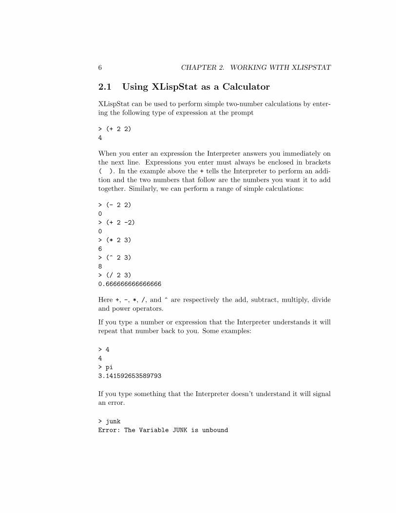
2.1 Using XLispStat as a Calculator
XLispStat can be used to perform simple two-number calculations by enter-ing the following type of expression at the prompt
> (+ 2 2)4
When you enter an expression the Interpreter answers you immediately onthe next line. Expressions you enter must always be enclosed in brackets( ). In the example above the + tells the Interpreter to perform an addi-tion and the two numbers that follow are the numbers you want it to addtogether. Similarly, we can perform a range of simple calculations:
> (- 2 2)0> (+ 2 -2)0> (* 2 3)6> (^ 2 3)8> (/ 2 3)0.666666666666666
Here +, -, *, /, and ^ are respectively the add, subtract, multiply, divideand power operators.
If you type a number or expression that the Interpreter understands it willrepeat that number back to you. Some examples:
> 44> pi3.141592653589793
If you type something that the Interpreter doesn’t understand it will signalan error.
> junkError: The Variable JUNK is unbound

2.1. USING XLISPSTAT AS A CALCULATOR 7
A number of additional operators that the Interpreter understands take,respectively, the natural logarithm, the exponent (ex) and the square rootof a number:
> (log 10)2.32585092994046> (exp 2)7.38905609893065> (sqrt 2)1.4142135623730951
In the above expressions log, exp and sqrt are functions that operate onthe numbers included to the right of them in the brackets. Also, the absolutevalue of a number can be obtained using the abs function as follows:
> (abs -3)3
The operators +, -, * and / can be applied to a sequence of numbers asfollows:
> (+ 1 2 3 4 5)15> (- 1 2 3 4 5)-13> (* 1 2 3 4 5)120> (/ 1 2 3).16666666666666
Notice that when we perform the operations +, -, * and / on a sequence ofnumbers the Interpreter performs the operation in sequence. For example,in the case of the subtract operator it subtracts the second number from thefirst, then subtracts the third number from what it obtained by subtractingthe second number from the first, then subtracts the fourth number fromthe number obtained in the previous subtraction, and so forth. In the caseof (/ 1 2 3), for example, it first divided 1 by 2 to get .5 and then divided.5 by 3 to get .16666666666.
The first principle of Lisp programing should now be clearly evident.When you send the XLispStat Interpreter a command asking it to do some-thing, the command must take the form of a set of brackets containing, inorder, the function you want the program to execute and the parametricinformation it needs to execute that function—that is

8 CHAPTER 2. WORKING WITH XLISPSTAT
(+ 2 3 1 4 5)
represents the statement
(<add><first number><second number><third number> ... etc.)
These operations can be nested. If we give the Interpreter the expression
> (+ 4 (/ 4 2))6
it first evaluates the expression in the nested brackets (/ 4 2), dividing thenumber 4 by the number 2, and then executes the + function in the mainbrackets to add that number to the number 4. We will henceforth refer tothe words or numbers that must be entered within the brackets after thefunction-name as the function’s arguments. The + function thus takes as itsarguments the numbers to be added together.
2.2 Defining Objects and Working with Lists
You can define objects using the def function in the following manner1
> (def num0 21)NUM0
> (def num1 (/ 4 2))NUM1
> (def num2 (+ 4 (/ 4 2)))NUM2
> (def word1 "junk")WORD1
To find out what objects present in the work space you simply apply thevariables function by executing the command
> (variables)NUM0 NUM1 NUM2 WORD1
1Actually, def is not really a function but a macro in ‘Lisp-speak’ but this need notconcern us.

2.2. DEFINING OBJECTS AND WORKING WITH LISTS 9
And to remind yourself of what an object is, simply type its name withoutsurrounding brackets and press return
> WORD1"junk"
Most of the work you will do with XLispStat will involve data taking theform of lists—indeed, the Lisp programming language, which is the basis ofXLispStat and of which Xlisp is a dialect, gets its name from its focus onLIStProcessing. We can define—that is, create—lists using the list functionas follows:
> (def numlist (list 1 2 -3 -4 5))NUMLIST> (def wrdlist (list "bob" "tom" "beatrice" "harry"))WRDLIST
To check the contents of these lists we would enter the commands
> numlist(1 2 -3 -4 5)> wrdlist("bob" "tom" "beatrice" "harry")
When we add, subtract, multiply or divide a number and a list, thatnumber is added to, subtracted from, multiplied by or divided by everynumber in the list—for example
> (+ 2 numlist)(3 4 -1 -2 7)> (- 2 numlist)(-1 0 -5 -6 3)> (* 2 numlist)(2 3 -6 -8 10)> (/ 2 numlist)(.5 1 -1.5 -2 2.5)
The same is true if we apply the abs, log or exp functions to a list—forexample 2
2The first command that follows is necessary because we cannot take the logarithm ofa negative number.

10 CHAPTER 2. WORKING WITH XLISPSTAT
> (def newlist (abs numlist))NEWLIST> (log newlist)(0.0 0.6931471805599453 1.0986122886681098 1.38629436111989061.6094379124341003)> (exp numlist)(2.718281828459045 7.38905609893065 0.049787068367863944 0.01831563888873418148.4131591025766)> (log (exp numlist))(1.0 2.0 -3.0 -4.0 5.0)
Other important functions produce from a list a single number. Amongthese are the functions sum, prod, max and min. For example,
> (def smallist (list 1 2 3 4))SMALLIST> smallist(1 2 3 4)> (sum smallist)10> (prod smallist)24> (max smallist)4> (min smallist)1
If we add, subtract, multiply or divide two lists, both of which must havethe same number of elements, we obtain a new list whose elements are thesum, difference, product or quotient of the corresponding elements of thetwo lists—for example
> newlist(1 2 3 4 5)> numlist(1 2 -3 -4 5)> (+ newlist numlist)(2 4 0 0 10)> (- newlist numlist)(0 0 6 8 0)
2.2. DEFINING OBJECTS AND WORKING WITH LISTS 11
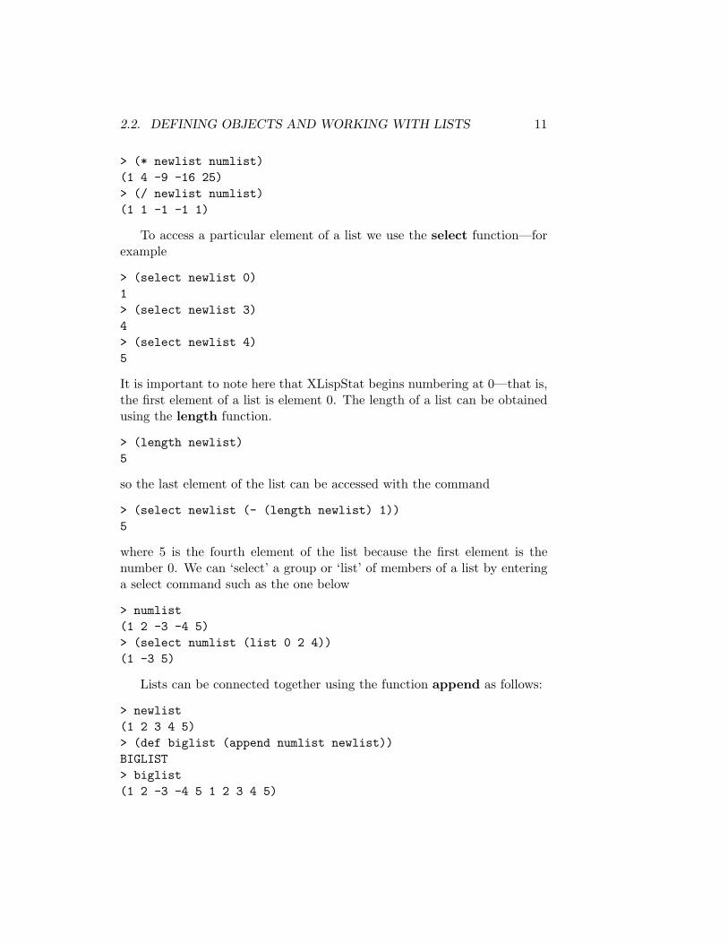
> (* newlist numlist)(1 4 -9 -16 25)> (/ newlist numlist)(1 1 -1 -1 1)
To access a particular element of a list we use the select function—forexample
> (select newlist 0)1> (select newlist 3)4> (select newlist 4)5
It is important to note here that XLispStat begins numbering at 0—that is,the first element of a list is element 0. The length of a list can be obtainedusing the length function.
> (length newlist)5
so the last element of the list can be accessed with the command
> (select newlist (- (length newlist) 1))5
where 5 is the fourth element of the list because the first element is thenumber 0. We can ‘select’ a group or ‘list’ of members of a list by enteringa select command such as the one below
> numlist(1 2 -3 -4 5)> (select numlist (list 0 2 4))(1 -3 5)
Lists can be connected together using the function append as follows:
> newlist(1 2 3 4 5)> (def biglist (append numlist newlist))BIGLIST> biglist(1 2 -3 -4 5 1 2 3 4 5)
12 CHAPTER 2. WORKING WITH XLISPSTAT
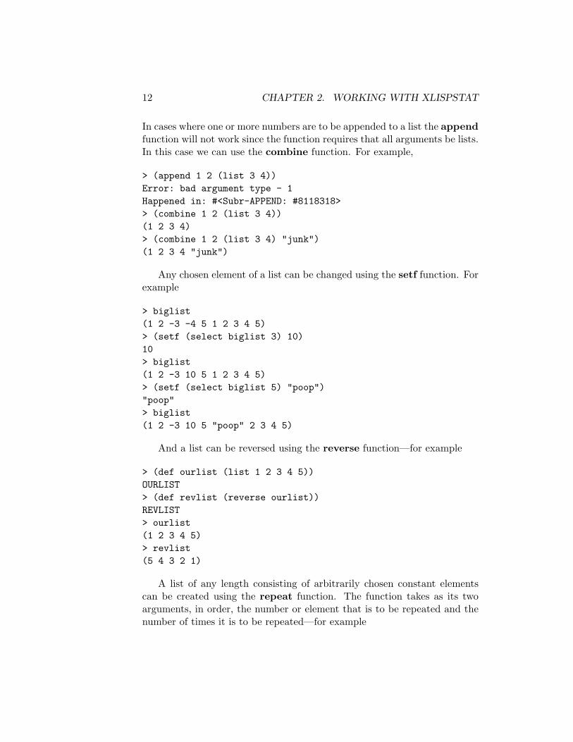
In cases where one or more numbers are to be appended to a list the appendfunction will not work since the function requires that all arguments be lists.In this case we can use the combine function. For example,
> (append 1 2 (list 3 4))Error: bad argument type - 1Happened in: #<Subr-APPEND: #8118318>> (combine 1 2 (list 3 4))(1 2 3 4)> (combine 1 2 (list 3 4) "junk")(1 2 3 4 "junk")
Any chosen element of a list can be changed using the setf function. Forexample
> biglist(1 2 -3 -4 5 1 2 3 4 5)> (setf (select biglist 3) 10)10> biglist(1 2 -3 10 5 1 2 3 4 5)> (setf (select biglist 5) "poop")"poop"> biglist(1 2 -3 10 5 "poop" 2 3 4 5)
And a list can be reversed using the reverse function—for example
> (def ourlist (list 1 2 3 4 5))OURLIST> (def revlist (reverse ourlist))REVLIST> ourlist(1 2 3 4 5)> revlist(5 4 3 2 1)
A list of any length consisting of arbitrarily chosen constant elementscan be created using the repeat function. The function takes as its twoarguments, in order, the number or element that is to be repeated and thenumber of times it is to be repeated—for example
2.2. DEFINING OBJECTS AND WORKING WITH LISTS 13
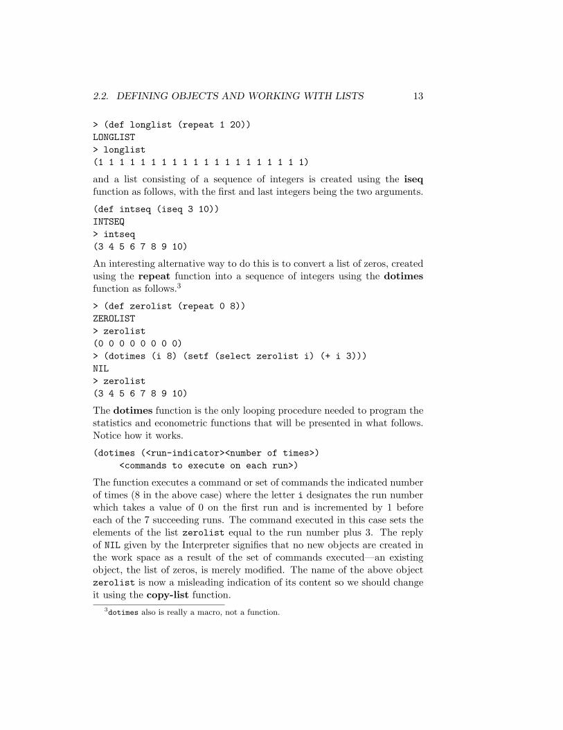
> (def longlist (repeat 1 20))LONGLIST> longlist(1 1 1 1 1 1 1 1 1 1 1 1 1 1 1 1 1 1 1 1)
and a list consisting of a sequence of integers is created using the iseqfunction as follows, with the first and last integers being the two arguments.
(def intseq (iseq 3 10))INTSEQ> intseq(3 4 5 6 7 8 9 10)
An interesting alternative way to do this is to convert a list of zeros, createdusing the repeat function into a sequence of integers using the dotimesfunction as follows.3
> (def zerolist (repeat 0 8))ZEROLIST> zerolist(0 0 0 0 0 0 0 0)> (dotimes (i 8) (setf (select zerolist i) (+ i 3)))NIL> zerolist(3 4 5 6 7 8 9 10)
The dotimes function is the only looping procedure needed to program thestatistics and econometric functions that will be presented in what follows.Notice how it works.
(dotimes (<run-indicator><number of times>)<commands to execute on each run>)
The function executes a command or set of commands the indicated numberof times (8 in the above case) where the letter i designates the run numberwhich takes a value of 0 on the first run and is incremented by 1 beforeeach of the 7 succeeding runs. The command executed in this case sets theelements of the list zerolist equal to the run number plus 3. The replyof NIL given by the Interpreter signifies that no new objects are created inthe work space as a result of the set of commands executed—an existingobject, the list of zeros, is merely modified. The name of the above objectzerolist is now a misleading indication of its content so we should changeit using the copy-list function.
3dotimes also is really a macro, not a function.
14 CHAPTER 2. WORKING WITH XLISPSTAT
> (def intlist1 (copy-list zerolist))INTLIST1
And we can now delete zerolist from the workspace using the undef func-tion
> (undef ’zerolist)ZEROLIST
The quotation mark ’ in front of the name zerolist tells the Interpreternot to perform any operation on the actual elements of the list—otherwise itwould expect the first element of the list to be a function and the remainingelements parameters required by that function.
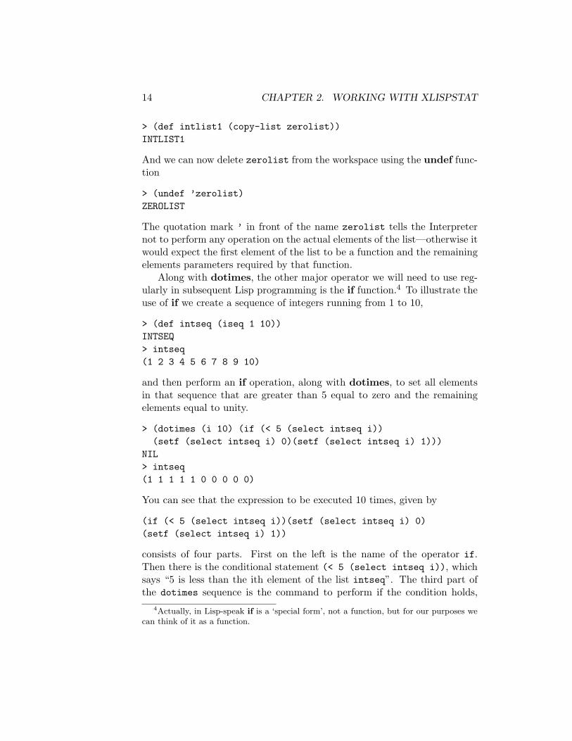
Along with dotimes, the other major operator we will need to use reg-ularly in subsequent Lisp programming is the if function.4 To illustrate theuse of if we create a sequence of integers running from 1 to 10,
> (def intseq (iseq 1 10))INTSEQ> intseq(1 2 3 4 5 6 7 8 9 10)
and then perform an if operation, along with dotimes, to set all elementsin that sequence that are greater than 5 equal to zero and the remainingelements equal to unity.
> (dotimes (i 10) (if (< 5 (select intseq i))(setf (select intseq i) 0)(setf (select intseq i) 1)))
NIL> intseq(1 1 1 1 1 0 0 0 0 0)
You can see that the expression to be executed 10 times, given by
(if (< 5 (select intseq i))(setf (select intseq i) 0)(setf (select intseq i) 1))
consists of four parts. First on the left is the name of the operator if.Then there is the conditional statement (< 5 (select intseq i)), whichsays “5 is less than the ith element of the list intseq”. The third part ofthe dotimes sequence is the command to perform if the condition holds,
4Actually, in Lisp-speak if is a ‘special form’, not a function, but for our purposes wecan think of it as a function.

2.2. DEFINING OBJECTS AND WORKING WITH LISTS 15
(setf (select intseq i) 0), which tells the Interpreter to set the ithelement equal to zero. And the fourth part of the statement is the commandto perform if the condition does not hold—set the ith element equal to unity.If we leave off the fourth part of the expression we get the following.
> (dotimes (i 10) (if (< 5 (select intseq i))(setf (select intseq i) 0)))
NIL> intseq(1 2 3 4 5 0 0 0 0 0)
Those elements that do not satisfy the condition are left unchanged. If wehad wanted to select the elements that are greater than or equal to 5 wewould have written the conditional statement as (<= 5 (select intseq i)).If we had wanted to set the condition to select the numbers 2 and 4, we wouldhave written the conditional statement as(if (or (= 2 (select intseq i))(= 4 (select intseq i)))).We could use and instead of or in the above but in that case no objectswould be selected.
Finally, we can also set up lists of lists. For example,
> (def triplist (list (list 1 3 4)(list 2 5 6)(list 7 0 7)))TRIPLIST> triplist((1 3 4) (2 5 6) (7 0 7))
Operations involving a single number and a list of lists, or taking the loga-rithm or exponent of a list of lists, perform the operation on every elementin the list of lists—for example
> (* 2 triplist)((2 6 8) (4 10 12) (14 0 14))
and an object in a particular list, say observation 2 of list 1, can be obtainedusing the select function in nested form—
> (select (select triplist 1) 2)6
In our econometric work we need to be able to examine portions of liststo make sure that the list we are accessing or using is the one we think weare using. Doing this with the select function is awkward. We also need tobe able to delete portions of lists. To perform these operations we need towrite our own Lisp functions, a task to which we now turn.
16 CHAPTER 2. WORKING WITH XLISPSTAT
2.3 Writing Lisp Functions
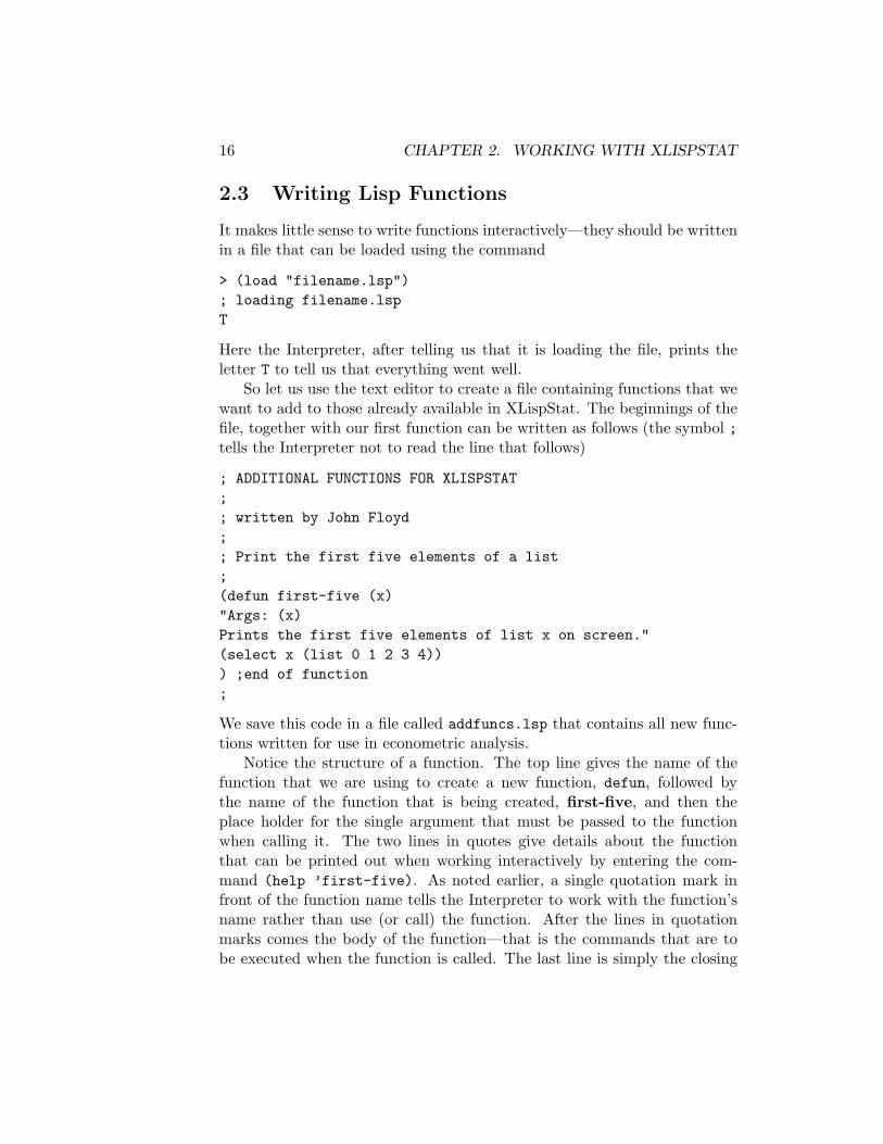
It makes little sense to write functions interactively—they should be writtenin a file that can be loaded using the command
> (load "filename.lsp"); loading filename.lspT
Here the Interpreter, after telling us that it is loading the file, prints theletter T to tell us that everything went well.
So let us use the text editor to create a file containing functions that wewant to add to those already available in XLispStat. The beginnings of thefile, together with our first function can be written as follows (the symbol ;tells the Interpreter not to read the line that follows)
; ADDITIONAL FUNCTIONS FOR XLISPSTAT;; written by John Floyd;; Print the first five elements of a list;(defun first-five (x)"Args: (x)Prints the first five elements of list x on screen."(select x (list 0 1 2 3 4))) ;end of function;
We save this code in a file called addfuncs.lsp that contains all new func-tions written for use in econometric analysis.
Notice the structure of a function. The top line gives the name of thefunction that we are using to create a new function, defun, followed bythe name of the function that is being created, first-five, and then theplace holder for the single argument that must be passed to the functionwhen calling it. The two lines in quotes give details about the functionthat can be printed out when working interactively by entering the com-mand (help ’first-five). As noted earlier, a single quotation mark infront of the function name tells the Interpreter to work with the function’sname rather than use (or call) the function. After the lines in quotationmarks comes the body of the function—that is the commands that are tobe executed when the function is called. The last line is simply the closing
2.3. WRITING LISP FUNCTIONS 17
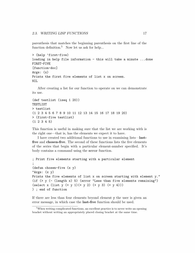
parenthesis that matches the beginning parenthesis on the first line of thefunction definition.5 Now let us ask for help...
> (help ’first-five)loading in help file information - this will take a minute ...doneFIRST-FIVE[function-doc]Args: (x)Prints the first five elements of list x on screen.NIL
After creating a list for our function to operate on we can demonstrateits use.
(def testlist (iseq 1 20))TESTLIST> testlist(1 2 3 4 5 6 7 8 9 10 11 12 13 14 15 16 17 18 19 20)> (first-five testlist)(1 2 3 4 5)
This function is useful in making sure that the list we are working with isthe right one—that is, has the elements we expect it to have.
I have created two additional functions to use in examining lists—last-five and chosen-five. The second of these functions lists the five elementsof the series that begin with a particular element-number specified. It’sbody contains a command using the error function.
; Print five elements starting with a particular element;(defun chosen-five (x y)"Args: (x y)Prints the five elements of list x on screen starting with element y."(if (> y (- (length x) 5) (error "Less than five elements remaining")(select x (list y (+ y 1)(+ y 2) (+ y 3) (+ y 4)))) ; end of function
If there are less than four elements beyond element y the user is given anerror message, in which case the last-five function should be used.
5When writing complicated functions, an excellent practice is to never write an openingbracket without writing an appropriately placed closing bracket at the same time.

18 CHAPTER 2. WORKING WITH XLISPSTAT
It is also convenient at times to shorten lists by removing elements at thebeginning or end, or even a particular element in the middle. Accordingly,I have written a series of five functions to do this. They are remove-first-element, remove-last-element, remove-first, remove-last andremove-selected-element. The first two of these functions take as theirsingle argument the list being modified. The second two functions take twoarguments: first, the number of elements to be removed, and second, the listfrom which they are to be removed. The last function takes as argumentsthe number of the element to be removed (numbering starts at zero) andthe list from which it is to be removed. To illustrate,
> testlist(1 2 3 4 5 6 7 8 9 10 11 12 13 14 15 16 17 18 19 20)> (remove-first-element testlist)(2 3 4 5 6 7 8 9 10 11 12 13 14 15 16 17 18 19 20)> (remove-last-element testlist)(1 2 3 4 5 6 7 8 9 10 11 12 13 14 15 16 17 18 19)> (remove-first 4 testlist)(5 6 7 8 9 10 11 12 13 14 15 16 17 18 19 20)> (remove-last 4 testlist)(1 2 3 4 5 6 7 8 9 10 11 12 13 14 15 16)> (remove-selected-element 10 testlist)(1 2 3 4 5 6 7 8 9 10 12 13 14 15 16 17 18 19 20)
With respect to the last case, where a selected element is removed, rememberthat in XLispStat numbering starts with the number zero.
To finish our discussion of the very basics of Lisp programing needed forour work we turn to the creation and manipulation of matrices.
2.4. WORKING WITH MATRICES 19
2.4 Working with Matrices
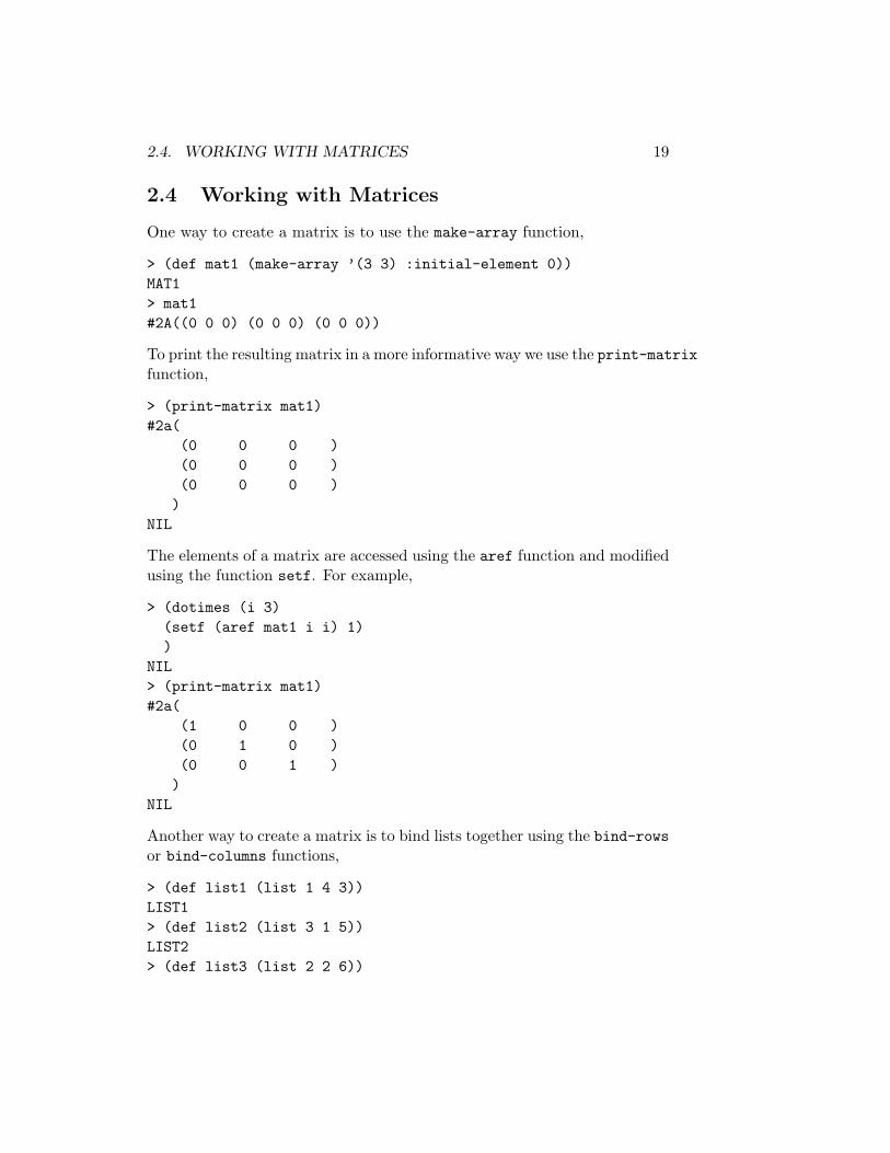
One way to create a matrix is to use the make-array function,
> (def mat1 (make-array ’(3 3) :initial-element 0))MAT1> mat1#2A((0 0 0) (0 0 0) (0 0 0))
To print the resulting matrix in a more informative way we use the print-matrixfunction,
> (print-matrix mat1)#2a(
(0 0 0 )(0 0 0 )(0 0 0 )
)NIL
The elements of a matrix are accessed using the aref function and modifiedusing the function setf. For example,
> (dotimes (i 3)(setf (aref mat1 i i) 1))
NIL> (print-matrix mat1)#2a(
(1 0 0 )(0 1 0 )(0 0 1 )
)NIL
Another way to create a matrix is to bind lists together using the bind-rowsor bind-columns functions,
> (def list1 (list 1 4 3))LIST1> (def list2 (list 3 1 5))LIST2> (def list3 (list 2 2 6))

20 CHAPTER 2. WORKING WITH XLISPSTAT
LIST3> (def list4 (list 1 5 2))LIST4> (def mat2 (bind-columns list1 list2 list3 list4))MAT2> (def mat3 (bind-rows list1 list2 list3 list4))MAT3> (print-matrix mat2)#2a(
(1 3 2 1 )(4 1 2 5 )(3 5 6 2 ))
NIL
> (print-matrix mat3)#2a(
(1 4 3 )(3 1 5 )(2 2 6 )(1 5 2 ))
NIL
The use of the diagonal function with a matrix as its argument returns thediagonal of that matrix
> (diagonal mat1)(1 1 1)> (diagonal mat2)(1 1 6)> (diagonal mat3)(1 1 6)
while the use of that function with a list as the argument produces a squarediagonal matrix with the list elements as the diagonal.

2.4. WORKING WITH MATRICES 21
> (def mat4 (diagonal (list 2 3 1)))MAT4> (print-matrix mat4)#2a(
(2 0 0 )(0 3 0 )(0 0 1 )
)NIL
Of the several ways to create an identity matrix, the easiest is to use theidentity-matrix function,
> (def identmat (identity-matrix 4))IDENTMAT> (print-matrix identmat)#2a(
(1 0 0 0 )(0 1 0 0 )(0 0 1 0 )(0 0 0 1 )
)NIL
A vector can be made by creating a list and coercing it into a vector usingthe coerce function,
> (def vec1 (coerce list5 ’vector))VEC1> vec1#(1 2 3 4)
or by simply using the vector function,
> (def vec2 (vector 2 3 1 4))VEC2> vec2#(2 3 1 4)
Vectors can be bound together in rows or columns to create matrices in thesame way as is done for lists. And matrices, too, can be bound together inthe same fashion—for example,
22 CHAPTER 2. WORKING WITH XLISPSTAT
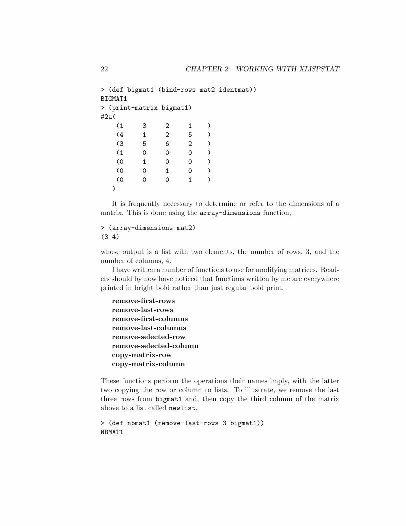
> (def bigmat1 (bind-rows mat2 identmat))BIGMAT1> (print-matrix bigmat1)#2a(
(1 3 2 1 )(4 1 2 5 )(3 5 6 2 )(1 0 0 0 )(0 1 0 0 )(0 0 1 0 )(0 0 0 1 ))
It is frequently necessary to determine or refer to the dimensions of amatrix. This is done using the array-dimensions function,
> (array-dimensions mat2)(3 4)
whose output is a list with two elements, the number of rows, 3, and thenumber of columns, 4.
I have written a number of functions to use for modifying matrices. Read-ers should by now have noticed that functions written by me are everywhereprinted in bright bold rather than just regular bold print.
remove-first-rowsremove-last-rowsremove-first-columnsremove-last-columnsremove-selected-rowremove-selected-columncopy-matrix-rowcopy-matrix-column
These functions perform the operations their names imply, with the lattertwo copying the row or column to lists. To illustrate, we remove the lastthree rows from bigmat1 and, then copy the third column of the matrixabove to a list called newlist.
> (def nbmat1 (remove-last-rows 3 bigmat1))NBMAT1

2.4. WORKING WITH MATRICES 23
> (print-matrix nbmat1)#2a(
(1 3 2 1 )(4 1 2 5 )(3 5 6 2 )(1 0 0 0 )
)
> (def newlist (copy-matrix-column 2 nbmat1))NEWLIST> newlist(2 2 6 0)
All these functions take two arguments. The first is the number of rows orcolumns or the row or column number, as the case may be, and the secondis the name of the matrix. Keep in mind that numbering always starts withrow zero, so that a request to copy or remove row 10 from a matrix actuallyleads to the copying or removal of the 11th row since the first row is rowzero.
Now we turn to the operations that can be performed on matrices. If twomatrices have the same dimensions, they can be added, subtracted, multi-plied and divided by each other in the same fashion as lists. For example
> (def bigmat2 (make-array ’(7 4) :initial-element 2))BIGMAT2> (print-matrix bigmat2)#2a(
(2 2 2 2 )(2 2 2 2 )(2 2 2 2 )(2 2 2 2 )(2 2 2 2 )(2 2 2 2 )(2 2 2 2 )
)NIL> (def bigmat3 (+ bigmat1 bigmat2))BIGMAT3

24 CHAPTER 2. WORKING WITH XLISPSTAT
> (print-matrix bigmat3)#2a(
(3 5 4 3 )(6 3 4 7 )(5 7 8 4 )(3 2 2 2 )(2 3 2 2 )(2 2 3 2 )(2 2 2 3 ))
NIL> (def bigmat4 (* bigmat1 bigmat2))BIGMAT4
> (print-matrix bigmat4)#2a(
( 2 6 4 2 )( 8 2 4 10 )( 6 10 12 4 )( 2 0 0 0 )( 0 2 0 0 )( 0 0 2 0 )( 0 0 0 2 ))
NIL
The latter operations are element-by-element.Standard multiplication of two conformable matrices is done using the
matmult function,
> (def mat5 (matmult mat2 mat3))MAT5> (print-matrix mat2)#2a(
(1 3 2 1 )(4 1 2 5 )(3 5 6 2 ))
NIL
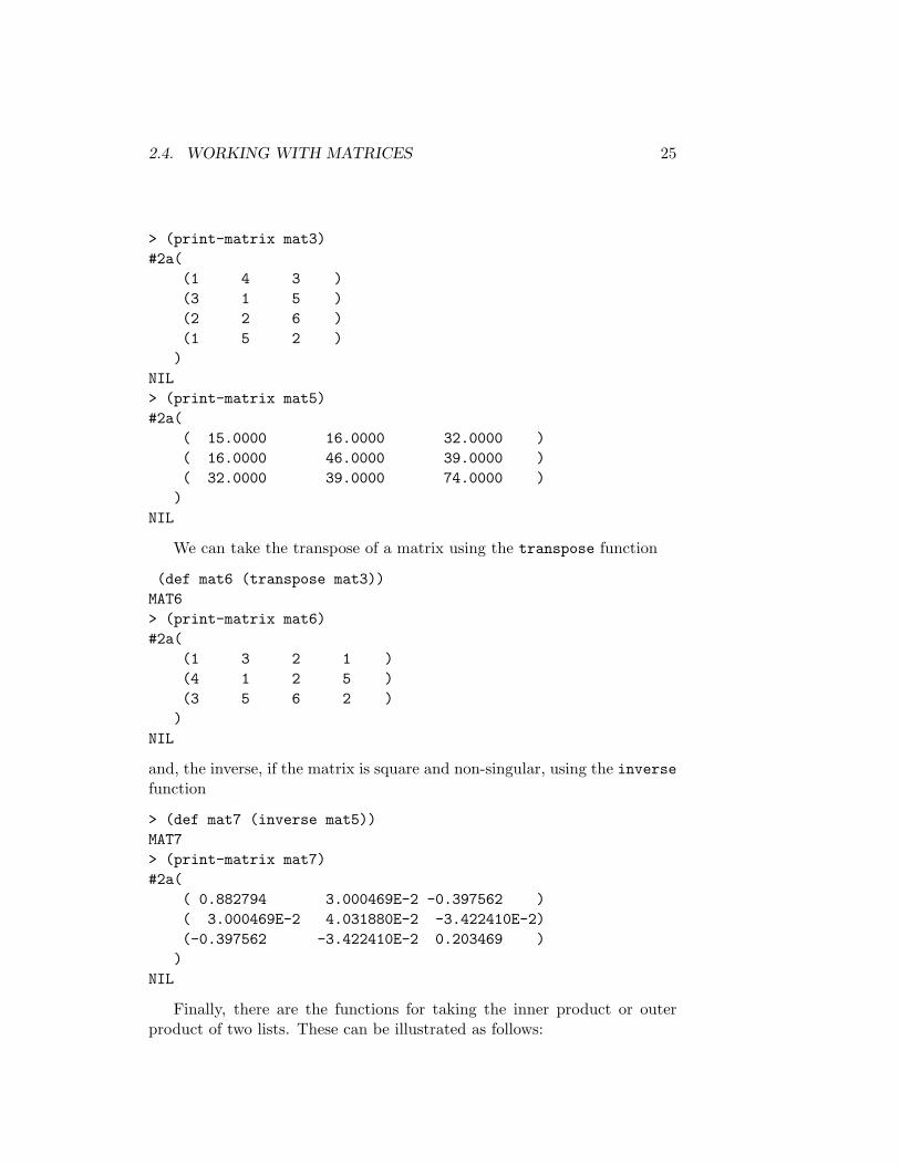
2.4. WORKING WITH MATRICES 25
> (print-matrix mat3)#2a(
(1 4 3 )(3 1 5 )(2 2 6 )(1 5 2 )
)NIL> (print-matrix mat5)#2a(
( 15.0000 16.0000 32.0000 )( 16.0000 46.0000 39.0000 )( 32.0000 39.0000 74.0000 )
)NIL
We can take the transpose of a matrix using the transpose function
(def mat6 (transpose mat3))MAT6> (print-matrix mat6)#2a(
(1 3 2 1 )(4 1 2 5 )(3 5 6 2 )
)NIL
and, the inverse, if the matrix is square and non-singular, using the inversefunction
> (def mat7 (inverse mat5))MAT7> (print-matrix mat7)#2a(
( 0.882794 3.000469E-2 -0.397562 )( 3.000469E-2 4.031880E-2 -3.422410E-2)(-0.397562 -3.422410E-2 0.203469 )
)NIL
Finally, there are the functions for taking the inner product or outerproduct of two lists. These can be illustrated as follows:
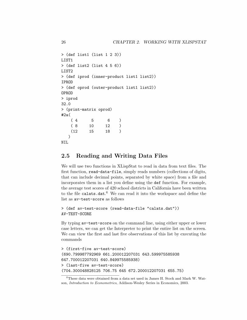
26 CHAPTER 2. WORKING WITH XLISPSTAT
> (def list1 (list 1 2 3))LIST1> (def list2 (list 4 5 6))LIST2> (def iprod (inner-product list1 list2))IPROD> (def oprod (outer-product list1 list2))OPROD> iprod32.0> (print-matrix oprod)#2a(
( 4 5 6 )( 8 10 12 )(12 15 18 ))
NIL
2.5 Reading and Writing Data Files
We will use two functions in XLispStat to read in data from text files. Thefirst function, read-data-file, simply reads numbers (collections of digits,that can include decimal points, separated by white space) from a file andincorporates them in a list you define using the def function. For example,the average test scores of 420 school districts in California have been writtento the file calats.dat.6 We can read it into the workspace and define thelist as av-test-score as follows
> (def av-test-score (read-data-file "calats.dat"))AV-TEST-SCORE
By typing av-test-score on the command line, using either upper or lowercase letters, we can get the Interpreter to print the entire list on the screen.We can view the first and last five observations of this list by executing thecommands
> (first-five av-test-score)(690.799987792969 661.200012207031 643.599975585938647.700012207031 640.849975585938)> (last-five av-test-score)(704.300048828125 706.75 645 672.200012207031 655.75)
6These data were obtained from a data set used in James H. Stock and Mark W. Wat-son, Introduction to Econometrics, Addison-Wesley Series in Economics, 2003.
2.5. READING AND WRITING DATA FILES 27
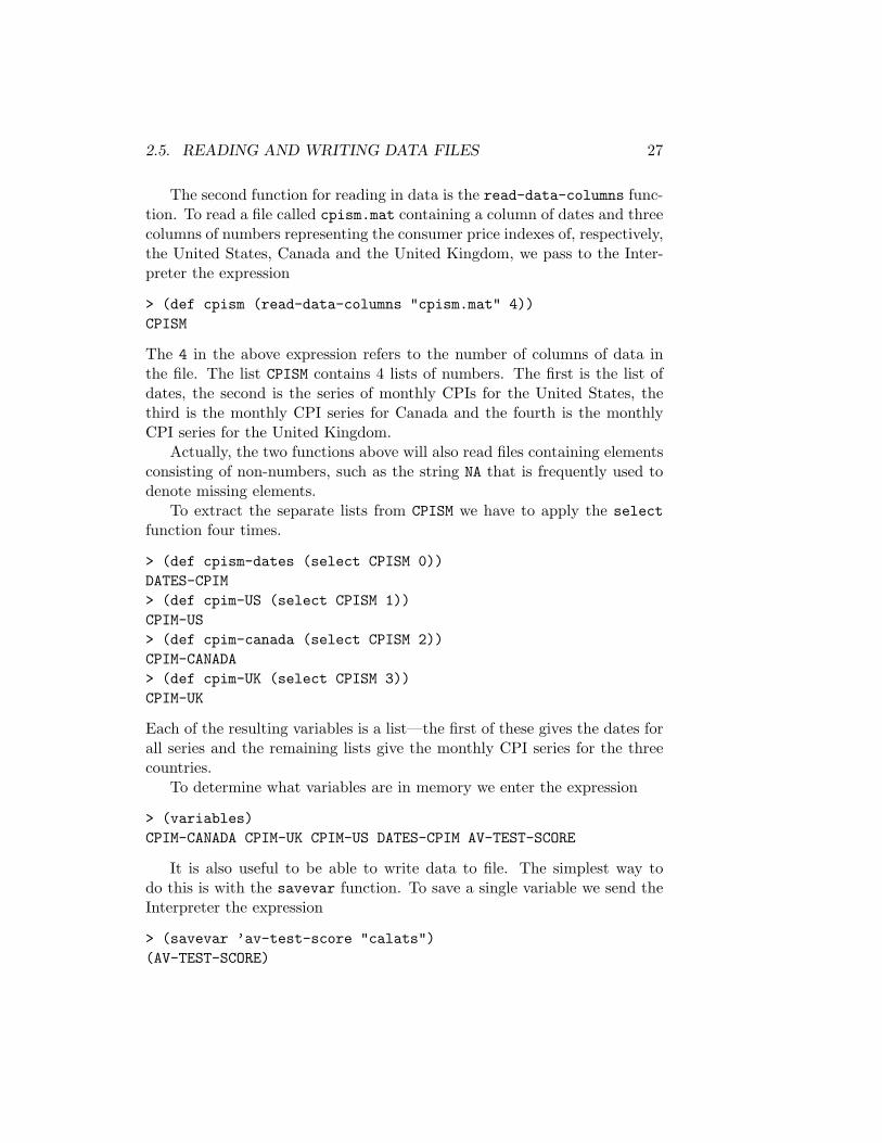
The second function for reading in data is the read-data-columns func-tion. To read a file called cpism.mat containing a column of dates and threecolumns of numbers representing the consumer price indexes of, respectively,the United States, Canada and the United Kingdom, we pass to the Inter-preter the expression
> (def cpism (read-data-columns "cpism.mat" 4))CPISM
The 4 in the above expression refers to the number of columns of data inthe file. The list CPISM contains 4 lists of numbers. The first is the list ofdates, the second is the series of monthly CPIs for the United States, thethird is the monthly CPI series for Canada and the fourth is the monthlyCPI series for the United Kingdom.
Actually, the two functions above will also read files containing elementsconsisting of non-numbers, such as the string NA that is frequently used todenote missing elements.
To extract the separate lists from CPISM we have to apply the selectfunction four times.
> (def cpism-dates (select CPISM 0))DATES-CPIM> (def cpim-US (select CPISM 1))CPIM-US> (def cpim-canada (select CPISM 2))CPIM-CANADA> (def cpim-UK (select CPISM 3))CPIM-UK
Each of the resulting variables is a list—the first of these gives the dates forall series and the remaining lists give the monthly CPI series for the threecountries.
To determine what variables are in memory we enter the expression
> (variables)CPIM-CANADA CPIM-UK CPIM-US DATES-CPIM AV-TEST-SCORE
It is also useful to be able to write data to file. The simplest way todo this is with the savevar function. To save a single variable we send theInterpreter the expression
> (savevar ’av-test-score "calats")(AV-TEST-SCORE)
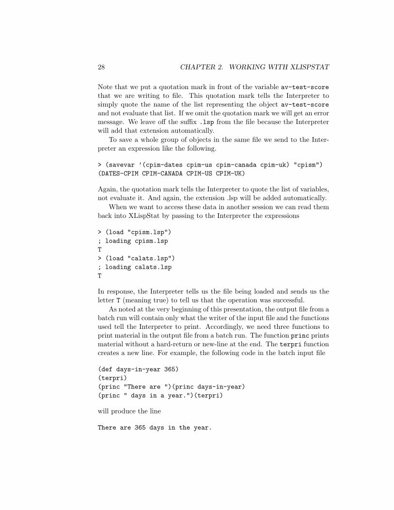
28 CHAPTER 2. WORKING WITH XLISPSTAT
Note that we put a quotation mark in front of the variable av-test-scorethat we are writing to file. This quotation mark tells the Interpreter tosimply quote the name of the list representing the object av-test-scoreand not evaluate that list. If we omit the quotation mark we will get an errormessage. We leave off the suffix .lsp from the file because the Interpreterwill add that extension automatically.
To save a whole group of objects in the same file we send to the Inter-preter an expression like the following.
> (savevar ’(cpim-dates cpim-us cpim-canada cpim-uk) "cpism")(DATES-CPIM CPIM-CANADA CPIM-US CPIM-UK)
Again, the quotation mark tells the Interpreter to quote the list of variables,not evaluate it. And again, the extension .lsp will be added automatically.
When we want to access these data in another session we can read themback into XLispStat by passing to the Interpreter the expressions
> (load "cpism.lsp"); loading cpism.lspT> (load "calats.lsp"); loading calats.lspT
In response, the Interpreter tells us the file being loaded and sends us theletter T (meaning true) to tell us that the operation was successful.
As noted at the very beginning of this presentation, the output file from abatch run will contain only what the writer of the input file and the functionsused tell the Interpreter to print. Accordingly, we need three functions toprint material in the output file from a batch run. The function princ printsmaterial without a hard-return or new-line at the end. The terpri functioncreates a new line. For example, the following code in the batch input file
(def days-in-year 365)(terpri)(princ "There are ")(princ days-in-year)(princ " days in a year.")(terpri)
will produce the line
There are 365 days in the year.

2.5. READING AND WRITING DATA FILES 29
on a new line with a hard-return at the end of that line. The third functionwe will use in presenting data is the format function. It is used in a functionwrite-matrix that I have written to write a matrix of numbers on the screenwithout the brackets that appear in the output from the print-matrixfunction.
;(defun write-matrix (x)"Args: (x)Prints a matrix on screen with format 12,3f."(def rcnum (array-dimensions x))(dotimes (i (select rcnum 0))(dotimes (j (select rcnum 1))(format t "~12,3f" (aref x i j))
) ; end dotimes j(terpri)) ; end dotimes i) ; end of function
In the expression (format t "~12,3f" (aref x i j)) the letter t tellsthe format function to print to the screen. The expression in quotations"~12,3f" is the control string containing a format directive (indicated bythe character ~) to create a field 12 characters long containing numbers indecimal notation (indicated by the trailing letter f) with 3 places to the rightof the decimal point. The final element (aref x i j) gives the number tobe placed in the 12 character field, namely the element of the ith row andjth column of the matrix x. A hard-return is not given by the formatcommand—the elements of the ith row of the matrix are printed in turnalong a line. After the ith row is completed the command (terpri) imposesa hard-return and dotimes i is then applied to row (i + 1) with j runningfrom zero to the number of columns of the matrix less 1.
More generally, the format function can be used to create a line ofnumbers without the use of dotimes. For example,
> (def num1 125)NUM1> (def num2 1)NUM2> (def num3 481.4563453)NUM3

30 CHAPTER 2. WORKING WITH XLISPSTAT
> (format t "~10,3f ~5,d ~15,e" num1 num2 num3)125.000 1 4.814563453E+2
NIL
The control string specifies that three numbers be printed, one a real numberwith 3 decimal places (10,3f) allocated 10 character-spaces, the second aninteger allocated five spaces (5,d) and the third using scientific notationallocated 15 spaces (15,e). The numbers follow the control string in theorder specified.
A data matrix can be augmented by creating a list of variable namesconsisting of a variable "obs" (or, alternatively, "date") plus the names ofthe variables in the columns of the matrix. Then the list of dates or a listof observation numbers created by the iseq function can be bound to thematrix
> (load "cpism.lsp"); loading cpism.lspT> (def varnames (list "DATE" "CPIUS" "CPICA" "CPIUK"))VARNAMES> (def datmat (bind-columns cpim-US cpim-Canada cpim-UK))DATMAT> (def newmat (bind-columns cpism-dates datmat))NEWMAT> (def cpidata (bind-rows varnames newmat))DATA> (write-matrix cpidata)DATE CPIUS CPICA CPIUK
1957.000 16.670 7.900 18.1401957.083 16.700 7.900 18.2201957.167 16.700 7.850 18.2601957.250 16.760 7.900 18.310
.. .. .. ..
.. .. .. ..
.. .. .. ..2002.750 115.630 119.350 118.9802002.833 115.920 119.550 118.9802002.917 115.540 119.750 118.710
NIL
The write-matrix function, when given strings (i.e., words), automaticallywrites them, left-justified, in place of numbers.

2.5. READING AND WRITING DATA FILES 31
In order to make data generated in XLispStat transferable to other pro-grams, I have written a write-matrix-to-file function, the code for whichis as follows:
(defun write-matrix-to-file (x y)"Args: (x y)Writes the matrix x to the file y."(setf f (open y :direction :output))(def rcnum (array-dimensions x))(dotimes (i (select rcnum 0))
(dotimes (j (select rcnum 1))(format f "~12,3f" (aref x i j))
) ; end dotimes j(terpri f)) ; end dotimes i(close f)) ; end of function
This differs from the write-matrix function in four respects. First the line(setf f (open y :direction :output)) opens a file called f within thefunction but given the name specified by y in the working directory to whichit is written, where the code-words :direction :output specify that we aregoing to be writing material to the file rather than reading from it. Second,the letter t immediately after the word format is changed to f to tell theInterpreter to write to the file rather than to the screen. Third, the command(terpri f) is used rather than just (terpri) to instruct the Interpreterto send the new line directive to the file rather than to the screen. And thecommand (close f) tells the Interpreter to close the file. The contents ofthe file will be exactly the same as what appears on the screen in responseto our using the write-matrix function. One could pretty-up the resultingfile with a text editor by adjusting the position of the labels. Alternatively,one could specify the labels in the varnames list with sufficient white spacebetween the initial quotation mark and the first letter of the variable nameto make the last character in each label the 12th character, thereby right-justifying the variable names. Without these modifications, however, the filecan be easily imported into a spreadsheet program or into another statisticalprogram.

32 CHAPTER 2. WORKING WITH XLISPSTAT
2.6 Transforming Data
Sometimes data have missing elements and contain numbers that are clearlyerroneous. These problems have to be fixed before we can proceed with ourwork. The obvious way to deal with these problems is in the spreadsheetfile from which we write the text matrix file that we subsequently readinto the workspace using the aforementioned read-data-columns function.Sometimes, however, it may be easier to use XLispStat, sometimes combinedwith our text editor, to handle some of these issues.
To illustrate we load in a data file on home mortgages used in Chap-ter 9 of the introductory econometrics text written by James Stock andMark Watson.7 The ultimate purpose is to use these data to determinewhether blacks are discriminated against in the granting of home mortgagesin Boston, U.S.A. The raw data were first organised in the spreadsheetfile hmdata.xls, then the block of numbers was written to the text matrixfile hmdata.mat and the list of variable names was written to the text filehmdata.lab and data descriptions were written to the text file hmdata.cat.The spreadsheet file was imported from a file of comma-separated-values,obtained from the Internet. For modern MS-Windows operating systems,as well as Linux, the free spreadsheet program Gnumeric, which is a clone ofMS-Excel, is available. This program reads files of comma-separated-valuesand can write spreadsheets to text matrix files. These data are described inhmdata.cat as follows.
OBS –Observation NumberRESULT –Decision (= 1 or 2 if approved, = 3 if denied (no other integers)AMT –Loan amount in ($ thousands)PROPVAL –Property Value in ($ thousands)RTDINC –Total debt payment obligations as percent of incomeRHDINC –Housing expense as percent of incomeCCSCORE –Consumer credit score (higher is worse)MCSCORE –Mortgage credit score (higher is worse)PUBBREC –Public bad record (1 if had past credit problems, 0 otherwise)DENMINS –Denied mortgage insurance (1 if denied, 0 otherwise)SELFEMP –Self employment status (= 1 if self-employed, zero otherwise)SINGLE –Martial status (= 1 if married, 2 if single and 3 if separated)SCHOOL –Years of schoolingUNRATE –Unemployment rate in applicants industryCONDO –Condominium (= 1, 2 = single family, 3 = families)RACE –Applicant’s race (black = 3, white = 5, no other integers)
7James H. Stock and Mark W. Watson, Introduction to Econometrics, Addison-Wesley,2003.
2.6. TRANSFORMING DATA 33
To reproduce the Stock and Watson presentation we need a variable, callit DENY, which will take a value of 1 if the mortgage application is denied and0 otherwise. The corresponding variable in the above dataset, RESULT, takesvalues of 1 and 2 if approved and 3 if denied. The martial status variable cantake three integer values, whereas Stock and Watson refer to it as 1 if marriedand 0 otherwise. The variable SCHOOL gives years of schooling whereas Stockand Watson use an alternative variable that takes a value of 1 if the persongraduated from high school and 0 otherwise. Similarly, the CONDO variabletakes three values where Stock and Watson have it taking only two, 1 if theresidence being mortgaged is a condominium and 0 otherwise. Finally, wewant the race variable to take a value of 1 if the person is black and 0 ifhe/she is white, rather than the above values of 3 if black and 5 if white.
Given the difficulty of fishing through a spreadsheet containing over 2300observations on 16 variables, the easiest way to fix all the above problemsis to read the data into the XLispStat workspace and then save it as a Lispfile, which is a text file that will appear in a correctly configured text editoras a list of horizontal lines of data, one line per variable, each extending farbeyond the right-most edge of the screen. The data can then be modifiedusing the text editor and then read back in to the workspace and furthermodified and re-saved. We work here in batch mode, which is the easiestway to do what has to be done.

34 CHAPTER 2. WORKING WITH XLISPSTAT
(def datlist (read-data-columns "hmdata.mat" 16))(def OBS (select datlist 0))(def RESULT (select datlist 1))(def AMT (select datlist 2))(def PROPVAL (select datlist 3))(def RTDINC (select datlist 4))(def RHDINC (select datlist 5))(def CCSCORE (select datlist 6))(def MCSCORE (select datlist 7))(def PUBREC (select datlist 8))(def DENMINS (select datlist 9))(def SELFEMP (select datlist 10))(def SINGLE (select datlist 11))(def SCHOOL (select datlist 12))(def UNRATE (select datlist 13))(def CONDO (select datlist 14))(def RACE (select datlist 15));(savevar ’(OBS RESULT AMT PROPVAL RTDINC RHDINC CCSCOREMCSCORE PUBREC DENMINS SELFEMP SINGLE SCHOOL UNRATECONDO RACE) "hmdatraw")
The Lisp file hmdatraw.lsp is a text file which when loaded into a text editorconfigured with no wrap-around will appear as follows, where the data offthe screen to the right can be viewed by pressing the right arrow key.
(DEF OBS (QUOTE (1 2 3 4 5 6 7 8 9 10 11 12 13 14 15 16 17 18(DEF RESULT (QUOTE (1 1 1 1 1 1 1 1 3 1 1 1 3 1 1 1 1 1 1 1 3(DEF AMT (QUOTE (88.0 118.0 185.0 185.0 330.0 97.0 56.0 187.0(DEF PROPVAL (QUOTE (110.0 128.0 201.0 215.0 550.0 190.0 75.0(DEF RTDINC (QUOTE (22.1 26.5 37.2 32.0 36.0 24.0 35.0 28.0 3(DEF RHDINC (QUOTE (22.1 26.5 24.8 25.0 35.0 17.0 29.0 22.0 2(DEF CCSCORE (QUOTE (5 2 1 1 1 1 1 2 2 2 1 1 1 1 1 2 1 2 2 2(DEF MCSCORE (QUOTE (2 2 2 2 1 1 2 2 2 1 2 2 2 1 1 1 1 1 2 2(DEF PUBREC (QUOTE (0 0 0 0 0 0 0 0 0 0 0 0 0 0 0 0 0 0 0 0 1(DEF DENMINS (QUOTE (0 0 0 0 0 0 0 0 1 0 0 0 1 0 0 0 0 0 0 0(DEF SELFEMP (QUOTE (0 0 0 0 0 0 0 0 0 0 0 0 0 0 0 0 0 0 0 0(DEF SINGLE (QUOTE (1 2 1 1 1 1 2 1 1 2 2 2 1 1 1 1 1 1 1 2 1(DEF SCHOOL (QUOTE (15 18 12 12 20 16 14 16 12 16 14 16 18 18(DEF UNRATE (QUOTE (3.9 3.2 3.2 4.3 3.2 3.9 3.9 1.8 3.1 3.9 3(DEF CONDO (QUOTE (2 2 2 2 2 2 1 2 2 2 1 2 2 2 2 2 2 2 2 2 2(DEF RACE (QUOTE (5 5 5 5 5 5 5 5 5 5 5 5 5 5 5 5 5 5 5 5 5 5

2.6. TRANSFORMING DATA 35
We can then use our text editor to search for and replace the relevant num-bers in the file. Each variable that needs to be operated on can be movedto the bottom line of the file and a search and replace done on it until allthe elements are appropriately 1 or 0. The next variable that needs actioncan then be moved to the bottom and the procedure repeated as appropri-ate. This procedure will not work, however, with the SCHOOL variable, whichtakes values ranging from 18 or more downward. But we can easily cleanup this variable as follows (again in batch mode) after reading the abovemodified data, now renamed hmdatadj.lsp back into the workspace andassuming that to complete high-school one must have at least 12 years ofschooling.
(load "hmdatadj")(dotimes (i (length school))(if (< (select school i) 12)(setf (select school i) 0)(setf (select school i) 1)) ; end if) ; end dotimes i
Upon further investigation, other problems appear. First, Stock and Watsonexpress the ratios of payments to income RTDINC and RHDINC as the frac-tions of income spent monthly on total debt-obligations and housing-debtobligations, respectively, whereas the data here are in percentages. This caneasily be taken care of using the following code.
(def rhdinc (/ rhdinc 100))(def rtdinc (/ rtdinc 100))
Then, it turns out, some of the values of the above two series exceed unity,implying that some people are spending much more than their income onhousing and/or total monthly debt charges! Since we have no way of findingout what is happening in these cases (the observed figures may be typos!)the best solution is to eliminate these observations from the data set. Theeasiest way to do this is to save the variables to a temporary Lisp file
> (savevar ’(RTDINC RHDINC) "tempvars")(RTDINC RHDINC)
and then, again using the text editor, replace all elements whose first twocharacters are the integer 1 plus a decimal point with the letters NA. Thenwe can read the revised data back into the workspace with the code

36 CHAPTER 2. WORKING WITH XLISPSTAT
> (load "tempvars"); loading tempvars.lspT
Now we have to eliminate from our data set all observations for whichone or more of the variables are NA. We do this using my find-NA-in-matrix function which takes as its sole argument the name of the matrixbeing searched. We must first bind all our variables together into a matrixusing bind-columns.
> (def datmat1 (bind-columns OBS AMT CCSCORE CONDO DENMINSMCSCORE PROPVAL PUBREC RACE RESULT RHDINC RTDINC SCHOOLSELFEMP SINGLE UNRATE))DATMAT1> (find-NA-in-matrix datmat1)
Missing valuerow column193 12210 12366 12411 12422 12458 12580 12599 12620 11692 12693 12693 14834 121094 101094 111106 121114 121140 121143 121144 121145 121148 121252 121320 111494 121619 12

2.6. TRANSFORMING DATA 37
1623 121631 121927 101927 111928 101928 112208 14
NIL
We need to delete the relevant rows, so we are only interested in the left-most column of numbers. And note that sometimes a row number appearstwice in the list! So we cut the above data from our XLispStat output fileusing the mouse and paste it in a temporary text file and then delete theright-most column and everything but the relevant row numbers with ourtext editor.8 Then we arrange the row numbers remaining after eliminatingduplications in the following list,
193 210 366 411 422 458 580 599 620 692 693 834 1094 1106 11141140 1143 1144 1145 1148 1252 1320 1494 1619 1623 1631 19271928 2208
and cut and paste them back into our batchfile and embed them in thefollowing code.
(def templist (list 193 210 366 411 422 458 580 599 620 692 693834 1094 1106 1114 1140 1143 1144 1145 1148 1252 1320 1494 16191623 1631 1927 1928 2208))(def nalist (reverse templist))(def newmat datmat1)(dotimes (i (length nalist))(remove-selected-row (select nalist i) newmat)) ; end dotimes i
It is important to note that we reverse the order of numbers before usingthem as an index of rows to be deleted from the renamed matrix newmat.If we were to proceed without reversing templist, deletion of element 193would cause the next NA element, 210, to now be the element 211 of theoriginal list! So we must delete the highest numbers first—changes in the
8The editor Joe, which is freely available for DOS and Linux, is one editor that candelete columns of numbers in a text file. The freely available Crimson Editor will do thisjob in modern MS-Windows operating systems.

38 CHAPTER 2. WORKING WITH XLISPSTAT
element numbers above the number of the element deleted then will not af-fect subsequent deletions. Finally, we have to extract into lists the variablesfrom the matrix newmat using the copy-matrix-column function and savethem in a Lisp file.
(def obs-adj (copy-matrix-column 0 newmat))(def amt (copy-matrix-column 1 newmat))(def ccscore (copy-matrix-column 2 newmat))(def condo (copy-matrix-column 3 newmat))(def denmins (copy-matrix-column 4 newmat))(def mcscore (copy-matrix-column 5 newmat))(def propval (copy-matrix-column 6 newmat))(def pubrec (copy-matrix-column 7 newmat))(def black (copy-matrix-column 8 newmat))(def deny (copy-matrix-column 9 newmat))(def rhdinc (copy-matrix-column 10 newmat))(def rtdinc (copy-matrix-column 11 newmat))(def school (copy-matrix-column 12 newmat))(def selfemp (copy-matrix-column 13 newmat))(def single (copy-matrix-column 14 newmat))(def unrate (copy-matrix-column 15 newmat))(savevar ’(OBS-ADJ DENY AMT PROPVAL RTDINC RHDINC CCSCOREMCSCORE PUBREC DENMINS SELFEMP SINGLE SCHOOL UNRATECONDO RACE) "hmdata")
In the process we rename the variable RESULT as DENY, consistent withthe terminology used by Stock and Watson. The variable OBS is renamedOBS-ADJ to take into account the fact that the deleted observation numberswill be missing from that list. This data set is now ready for the analysisthat will be the subject of Chapter 8.
When working with time-series data we need to incorporate dates for theseries. As should be evident from the monthly data above, my conventionis to enumerate quarterly data as, for example,
1990.00 1990.25 1990.50 1990.75and monthly data as
1990.000 1990.083 1990.167 1990.250 1990.333 1990.4171990.500 1990.583 1990.667 1990.750 1990.833 1990.917
with the dates for annual data, of course, consisting entirely of integers.When it is inconvenient to construct in our spreadsheet program a datelist
consisting of real numbers of the sort above we can simply save the ma-trix of variables, ignoring the dates, as a text file and read it into the

2.6. TRANSFORMING DATA 39
XLispStat workspace using read-data-columns and then construct thedatelist in XLispStat using my setdates function. This function takes threearguments—in order, the series for which the datelist is to be created (anyvariable in the original matrix will do), the date of the first observation, andthe frequency, which will be 1 for annual data, 4 for quarterly data and 12for monthly data. To illustrate this and some additional useful functions forworking with time series, we read in the file uscpim.lsp, which contains asits only variable the monthly U.S. consumer price index. The file alreadyincludes a datelist but, for illustrative purposes, we construct a new one.The first observation is for March 1962—we have to know this fact to makea datelist.
> (load "uscpim.lsp"); loading uscpim.lsp"T> (load "addfuncs.lsp"); loading addfuncs.lspT>(variables)(DATESMO USCPIM)> (def newdates (setdates uscpim 1962.167 12))NEWDATES> (Variables)(DATELIST DATESMO NEWDATES USCPIM)> (first-five newdates)(1962.167 1962.2503333333332 1962.3336666666667 1962.4171962.5003333333332)> (first-five datesmo)(1962.167 1962.25 1962.333 1962.417 1962.5)> (first-five datelist)(1962.167 1962.2503333333332 1962.3336666666667 1962.4171962.5003333333332)> (last-five newdates)(2005.5836666666667 2005.667 2005.75033333333322005.8336666666667 2005.917)> (last-five datesmo)(2005.583 2005.667 2005.75 2005.833 2005.917)> (last-five datelist)(2005.5836666666667 2005.667 2005.75033333333322005.8336666666667 2005.917)
40 CHAPTER 2. WORKING WITH XLISPSTAT
The variable DATELIST in the workspace is left there by the setdates func-tion. Assigning this generic name to a datelist in our research runs the riskthat it will subsequently be over-written when that function is called again.Another frequent requirement is to change the base of a series. Suppose,
for example, that we want to change the base of uscpim to 1963-66 = 100.We use my base function, which takes four arguments—first, the time-serieslist being put on a new base, then the datelist to which the series conforms,then the beginning date of the new base period, and finally, the number ofperiods in the new base period.
> (def cpim (base uscpim newdates 1963.0 48))CPIM
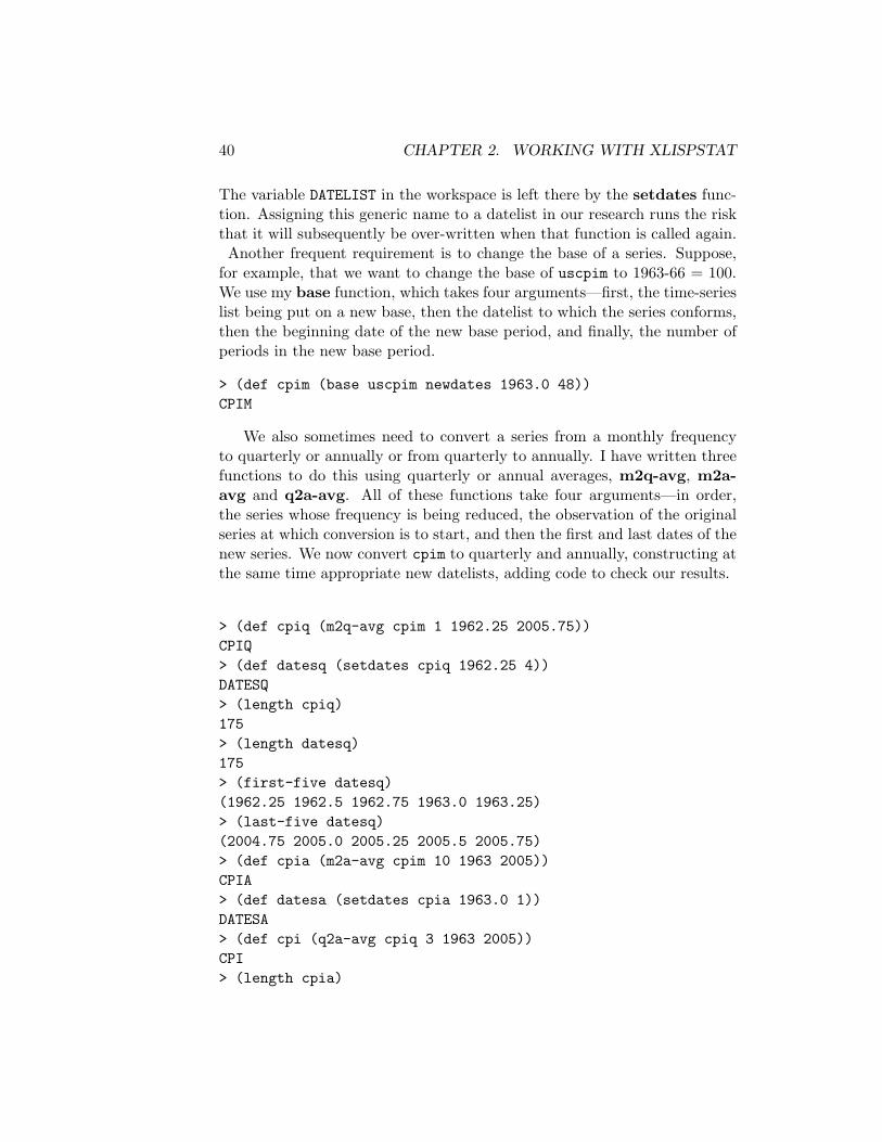
We also sometimes need to convert a series from a monthly frequencyto quarterly or annually or from quarterly to annually. I have written threefunctions to do this using quarterly or annual averages, m2q-avg, m2a-avg and q2a-avg. All of these functions take four arguments—in order,the series whose frequency is being reduced, the observation of the originalseries at which conversion is to start, and then the first and last dates of thenew series. We now convert cpim to quarterly and annually, constructing atthe same time appropriate new datelists, adding code to check our results.
> (def cpiq (m2q-avg cpim 1 1962.25 2005.75))CPIQ> (def datesq (setdates cpiq 1962.25 4))DATESQ> (length cpiq)175> (length datesq)175> (first-five datesq)(1962.25 1962.5 1962.75 1963.0 1963.25)> (last-five datesq)(2004.75 2005.0 2005.25 2005.5 2005.75)> (def cpia (m2a-avg cpim 10 1963 2005))CPIA> (def datesa (setdates cpia 1963.0 1))DATESA> (def cpi (q2a-avg cpiq 3 1963 2005))CPI> (length cpia)
2.6. TRANSFORMING DATA 41
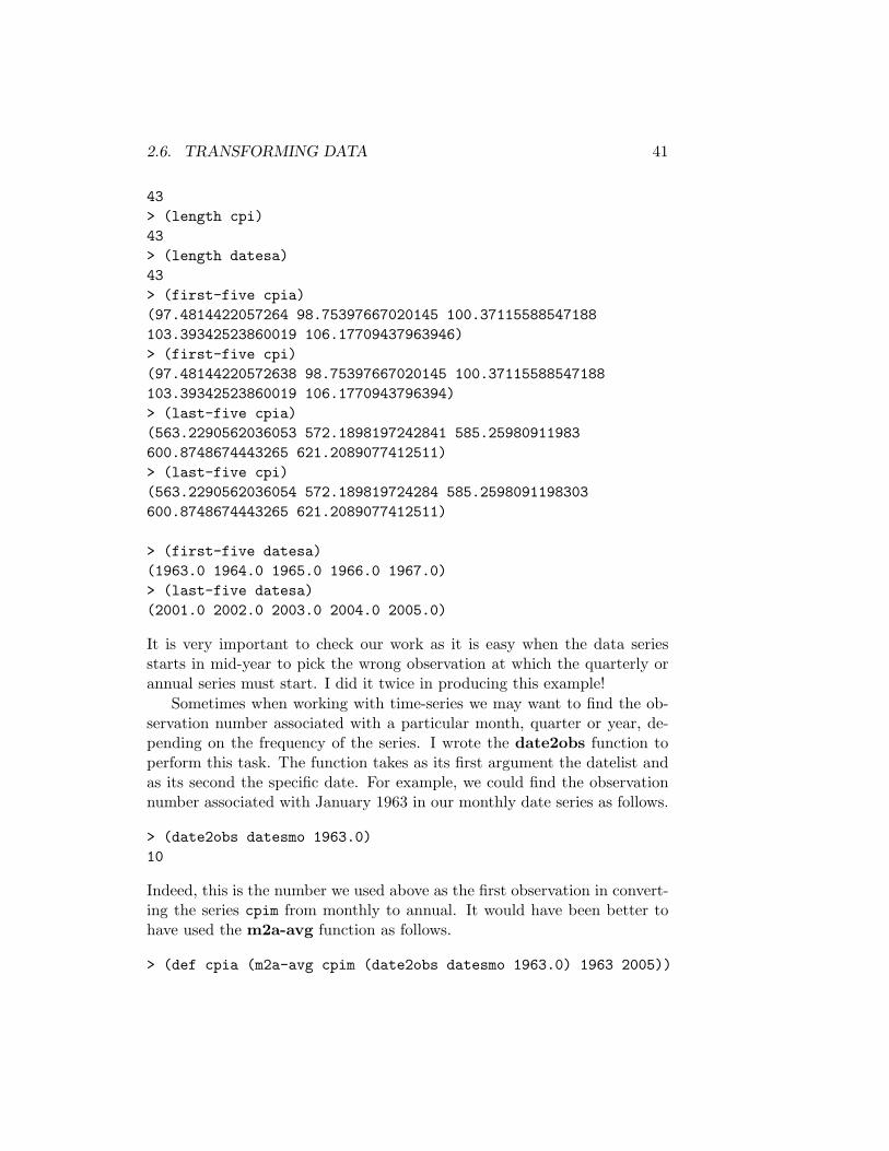
43> (length cpi)43> (length datesa)43> (first-five cpia)(97.4814422057264 98.75397667020145 100.37115588547188103.39342523860019 106.17709437963946)> (first-five cpi)(97.48144220572638 98.75397667020145 100.37115588547188103.39342523860019 106.1770943796394)> (last-five cpia)(563.2290562036053 572.1898197242841 585.25980911983600.8748674443265 621.2089077412511)> (last-five cpi)(563.2290562036054 572.189819724284 585.2598091198303600.8748674443265 621.2089077412511)
> (first-five datesa)(1963.0 1964.0 1965.0 1966.0 1967.0)> (last-five datesa)(2001.0 2002.0 2003.0 2004.0 2005.0)
It is very important to check our work as it is easy when the data seriesstarts in mid-year to pick the wrong observation at which the quarterly orannual series must start. I did it twice in producing this example!
Sometimes when working with time-series we may want to find the ob-servation number associated with a particular month, quarter or year, de-pending on the frequency of the series. I wrote the date2obs function toperform this task. The function takes as its first argument the datelist andas its second the specific date. For example, we could find the observationnumber associated with January 1963 in our monthly date series as follows.
> (date2obs datesmo 1963.0)10
Indeed, this is the number we used above as the first observation in convert-ing the series cpim from monthly to annual. It would have been better tohave used the m2a-avg function as follows.
> (def cpia (m2a-avg cpim (date2obs datesmo 1963.0) 1963 2005))
42 CHAPTER 2. WORKING WITH XLISPSTAT
Another frequent task is detrending a time-series. We can do this withmy detrend function which takes as its single argument the series-list tobe detrended, generates the resulting detrended series detseries and alsoleaves in memory the trend of the series as the list trendfit. We detrendour cpiq series, and check our results, using the following code.
> (def detcpiq (detrend cpiq))DETCPIQ> (def trndcpiq trendfit)TRNDCPIQ
> (def diftrnd (difference trndcpiq))DIFTRND> (first-five diftrnd)(3.383710504582993 3.383710504582993 3.3837105045829933.383710504582993 3.383710504582993)> (last-five diftrnd)(3.383710504583064 3.3837105045829503 3.3837105045830643.3837105045829503 3.3837105045829503)> (plot-lines (- datesq 1900) detcpiq)#<Object: 82cd128, prototype = SCATTERPLOT-PROTO>
We take the first-difference of the resulting trend and plot the detrendedseries to make sure we did not make a coding error.
When working with time series it is often necessary to make many leadsand lags of a variable. I have written two functions for this purpose, block-lead and block-lag. Both functions take two arguments—first, the seriesfor which leads or lags are to be obtained, and second, the number of leadsor lags. The block-lag leaves two objects in the workspace, laglist andlagmat. The former is a list of the current and lagged series, in that order,and the latter is a matrix of the lagged series with the one-period lag in theleft-most column and the maximum lag requested in the right-most column.The latter object is returned by the function in the sense that one can writethe code
> (def lagged-cpiq (block-lag cpiq 10))LAGGED-INFCA
to give the matrix a name other than lagmat. To give a name other thanlaglist to the list of current and lagged series one has to use the copy-listfunction. The objects in the workspace will be overwritten on the next occa-sion that the function is used or when another unrelated function happens
2.6. TRANSFORMING DATA 43
to leave objects having those names in the workspace. The block-leadfunction also leaves two objects in the workspace, leadlist and leadmat.The former is a list of the leads and current series while the latter, which isreturned by the function, is a matrix of lead series. These objects have themaximum lead of the series on the extreme-left of the list or matrix and thecurrent value of the series as the right-most list or matrix column.
To conveniently set up time-series variables for OLS regression analysis,I wrote the set-time-series function which takes four arguments in thefollowing order—the series being prepared for future regressions, the datelistto which that series conforms, the beginning date at which subsequent OLS-regressions will begin, the date at which those regressions will end, and thenumber of lags of the series to be included. Where the number of lagsspecified exceeds zero the function calls the block-lag function discussedabove and returns the matrix of lagged values created by that function,leaving it in the workspace along with the list of current and lagged valuescalled laglist. The function also leaves in the workspace a datelist calledadjdates which conforms to the rows of the matrix of lagged values and thelists contained in laglist.
> (def cpilmat (set-time-series cpiq datesq 1974.0 2000.75 8))CPILMAT> (array-dimensions cpilmat)(108 8)> (length laglist)9> (def row1 (copy-matrix-row 0 cpilmat))ROW1> row1(146.1293743372216 142.5238600212089 139.7667020148462136.90349946977727 134.78260869565216 133.4040296924708132.34358430540826 131.4952279957582)> (first-five (select laglist 0))(150.4772004241781 154.50689289501588 158.85471898197238163.73276776246018 167.23223753976666)> (first-five (select laglist 1))(146.1293743372216 150.4772004241781 154.50689289501588158.85471898197238 163.73276776246018)> (first-five (select laglist 2))(142.5238600212089 146.1293743372216 150.4772004241781154.50689289501588 158.85471898197238)
44 CHAPTER 2. WORKING WITH XLISPSTAT
> (first-five (select laglist 3))(139.7667020148462 142.5238600212089 146.1293743372216150.4772004241781 154.50689289501588)> (first-five adjdates)(1974.0 1974.25 1974.5 1974.75 1975.0)> (last-five adjdates)(1999.75 2000.0 2000.25 2000.5 2000.75)
The lengths of all these lists equal the number of rows in the matrix of laggedvalues and they all conform to the datelist adjdates which represents theperiod over which the regression will be run. The series that represents thefirst argument in the function is not modified by the function although thefirst series in laglist is a modified version of it. A modification of the seriesthat will make it equivalent to the first list in laglist can be performed byusing the set-time-series function specifying 0 lags.
> (def newcpiq (set-time-series cpiq datesq 1974.0 2000.75 0))NEWCPIQ> (first-five newcpiq)(150.4772004241781 154.50689289501588 158.85471898197238163.73276776246018 167.23223753976666)
In this case the function returns a list rather than a matrix. If a non-contiguous set of lags is to be included in an OLS regression, we simplyextract from laglist and bind together the particular lags we want toinclude.
An alternative way to lag a series is simply to delete elements from theend of it and make the original series conform to the lagged one by deletingan equivalent number of elements from its beginning. For example, supposewe want to calculate monthly the year-over-year U.S. CPI inflation rate. Wecreate a 12-month lag of the series by deleting the last 12 observations andthen shorten the original series to conform to the 12-month lagged one bydeleting its first 12 observations. We then make a new datelist by deletingthe first 12 observations from the original date list. Finally, we calculate thepercentage excess of the adjusted original series over the 12-month laggedversion.
> (def cpi-12 (remove-last 12 uscpim))CPI-12> (def adjcpi (remove-first 12 uscpim))ADJCPI
2.6. TRANSFORMING DATA 45
> (def adjdates (remove-first 12 datesmo))ADJDATES> (first-five datesmo)(1962.167 1962.25 1962.333 1962.417 1962.5)> (first-five adjdates)(1963.167 1963.25 1963.333 1963.417 1963.5)> (def infyy (* 100 (/ (- adjcpi cpi-12) cpi-12)))INFYY> (first-five infyy)(0.9933774834437109 0.9933774834437109 0.99337748344371091.3245033112582854 1.6556291390728477)
> (last-five infyy)(3.590285110876443 4.69161834475488 4.3501048218029253.451882845188296 3.3995815899581596)
An alternative way to calculate the year-over-year inflation rate would be totake 100 times the difference in the logarithms of the adjusted current and12-month lagged series.
> (def altinfyy (* 100 (- (log adjcpi)(log cpi-12))))ALTINFYY> (first-five altinfyy)(0.9884759232542173 0.9884759232542173 0.98847592325421731.3158084577511442 1.6420730212327594)> (last-five altinfyy)(3.5273366379285243 4.584887467010379 4.2581452055964423.3936418571311577 3.3430729559270844)
The results are slightly different, reflecting the fact that relative differencesare not precisely equal to the difference of the logarithms.
Finally, we occasionally need to create monthly or quarterly seasonaldummy variables to cope with seasonality in our data. I have written twofunctions to do this, seasdums-M and seasdums-Q. Both of these func-tions take two arguments. The first is the datelist to which the variablesconform and the second is the number of the month (starting from 1 forJanuary or for the first quarter) which will be given by the first observationin the datelist. For example, to create monthly seasonal dummies for ouruscpim series we would first check the datelist to determine the month ofthe first observation and then apply the seasdums-M function.

46 CHAPTER 2. WORKING WITH XLISPSTAT
> (first-five datesmo)(1962.167 1962.25 1962.333 1962.417 1962.5)> (seasdums-M datesmo 3)MD11
The function leaves eleven seasonal dummies in the workspace.MD1 MD2 MD3 MD4 MD5 MD6 MD7 MD8 MD9 MD10 MD11
The dummy for December is missing and the seasonal for that month will beincorporated in the constant term of the regressions in which these dummyvariables are included. To construct quarterly dummies we execute the lineof code
> (seasdums-Q datesq 2)QD3
which leaves the three quarterly dummies QD1, QD2 and QD3 in the workspace.The seasonal effect associated with the fourth dummy will be incorporatedinto the constant term in regressions in which these dummy variables arepresent.
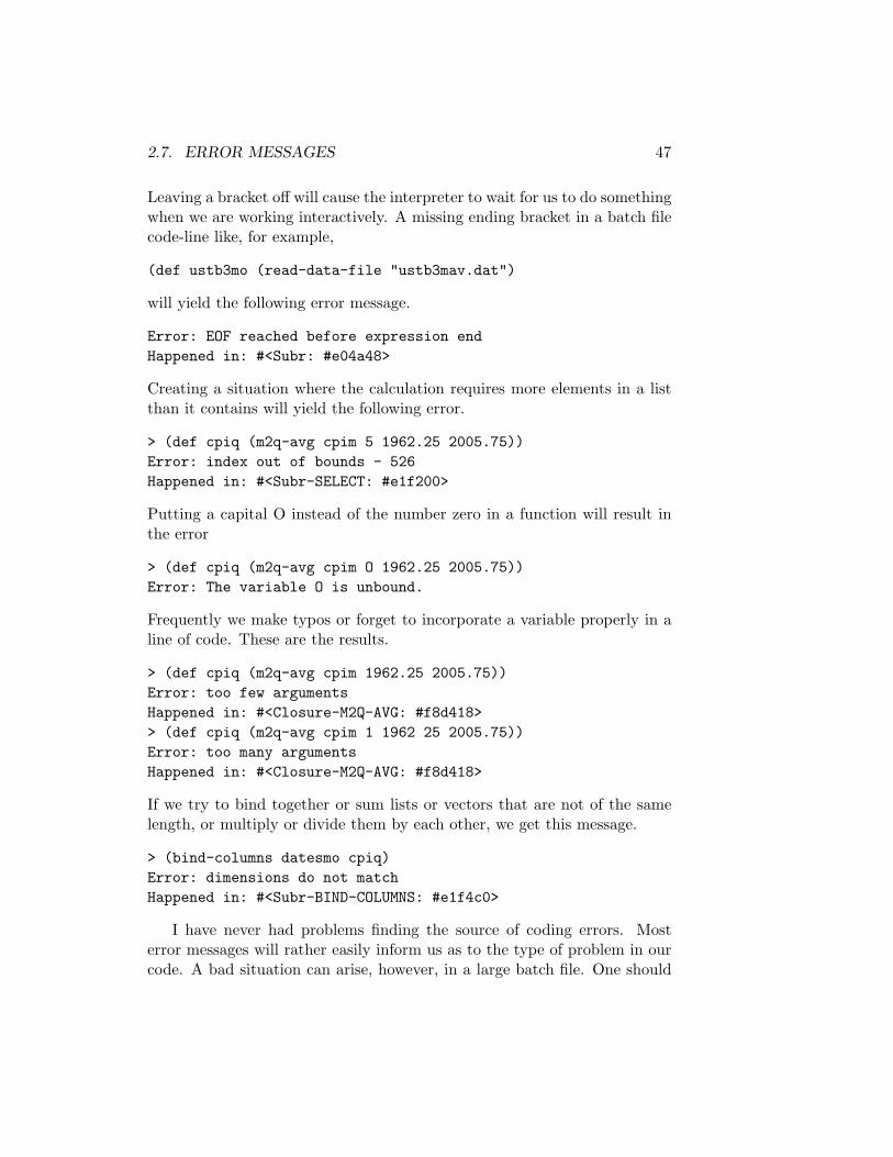
2.7 Error Messages
In ending this chapter it is important to examine the types of error messagesone is likely to receive when writing XLispStat code. Leaving brackets off acommand that requires them will yield the following error.
> variablesError: The variable VARIABLES is unbound.
The Interpreter does not recognise a function when the brackets are left off.Alternatively, if we put brackets around a variable that the Interpreter doesrecognise, it will think that it is a function.
> (uscpim)Error: The function USCPIM is not defined.
If we put an extra bracket on the end of an expression we will get thefollowing error message.
> (def adjcpi (remove-first 12 uscpim)))ADJCPI>Error: misplaced close parenHappened in: #<Subr: #e04a28>
2.7. ERROR MESSAGES 47
Leaving a bracket off will cause the interpreter to wait for us to do somethingwhen we are working interactively. A missing ending bracket in a batch filecode-line like, for example,
(def ustb3mo (read-data-file "ustb3mav.dat")
will yield the following error message.
Error: EOF reached before expression endHappened in: #<Subr: #e04a48>
Creating a situation where the calculation requires more elements in a listthan it contains will yield the following error.
> (def cpiq (m2q-avg cpim 5 1962.25 2005.75))Error: index out of bounds - 526Happened in: #<Subr-SELECT: #e1f200>
Putting a capital O instead of the number zero in a function will result inthe error
> (def cpiq (m2q-avg cpim O 1962.25 2005.75))Error: The variable O is unbound.
Frequently we make typos or forget to incorporate a variable properly in aline of code. These are the results.
> (def cpiq (m2q-avg cpim 1962.25 2005.75))Error: too few argumentsHappened in: #<Closure-M2Q-AVG: #f8d418>> (def cpiq (m2q-avg cpim 1 1962 25 2005.75))Error: too many argumentsHappened in: #<Closure-M2Q-AVG: #f8d418>
If we try to bind together or sum lists or vectors that are not of the samelength, or multiply or divide them by each other, we get this message.
> (bind-columns datesmo cpiq)Error: dimensions do not matchHappened in: #<Subr-BIND-COLUMNS: #e1f4c0>
I have never had problems finding the source of coding errors. Mosterror messages will rather easily inform us as to the type of problem in ourcode. A bad situation can arise, however, in a large batch file. One should

48 CHAPTER 2. WORKING WITH XLISPSTAT
never write more than a few lines of code without processing the batch file tocheck for errors. Make sure that each little section of code is correct beforeproceeding. And any time a line or two of code in the middle of a batch fileis changed, check that the programming is correct by processing the file. Aterrible situation arises when there is an error somewhere in a big file, withlittle indication as to its location. Should this happen, the best procedureis not to go through the file line-by-line to try to find the error. Rather, oneshould simply insert one’s favourite profanity at some point in the file andprocess it. If the Interpreter hangs up on your profanity, the error in the fileis below it. Move the profanity down a few lines and try again. When theerror appears before the objection to your profanity you will know that it isabove the point where the profanity was inserted.
Always keep backups of function files and batch files that work properly.Then, if a character is accidentally inserted somewhere in the file when youare working on it you can always simply replace the file with its backup.
I have been rather sloppy in allowing the functions I have created to leaveobjects in the workspace. The danger is that these objects may overwritean object of the same name that we want to maintain intact for futurereference. But, as yet, I have never had this problem. The reason, I believe,is that I never use generic names for variables in my batch code files, likevar1 or lastvar or newvar, and I never allow any functions I write to leavevariables with names containing characters with economic meaning like, forexample, cpi or gdp, in the workspace. The descriptions surrounded byquotation marks in the function definitions in the file addfuncs.lsp, whichare accessible by looking in the file with a text editor or by applying the helpfunction in an XLispStat session, note any objects required in the workspaceby each particular function and list any variables each function leaves in theworkspace. If there is any question about whether a variable of importanceis likely to be over-written, one should check there.
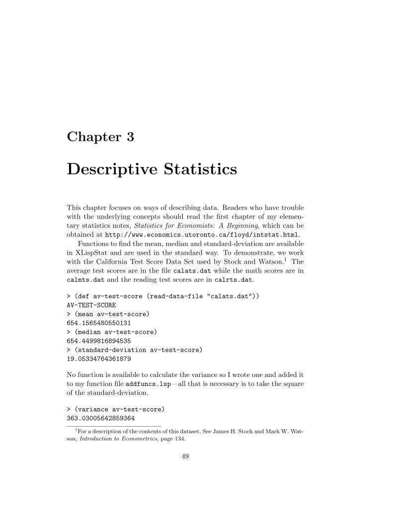
Chapter 3
Descriptive Statistics
This chapter focuses on ways of describing data. Readers who have troublewith the underlying concepts should read the first chapter of my elemen-tary statistics notes, Statistics for Economists: A Beginning, which can beobtained at http://www.economics.utoronto.ca/floyd/intstat.html.
Functions to find the mean, median and standard-deviation are availablein XLispStat and are used in the standard way. To demonstrate, we workwith the California Test Score Data Set used by Stock and Watson.1 Theaverage test scores are in the file calats.dat while the math scores are incalmts.dat and the reading test scores are in calrts.dat.
> (def av-test-score (read-data-file "calats.dat"))AV-TEST-SCORE> (mean av-test-score)654.1565480550131> (median av-test-score)654.4499816894535> (standard-deviation av-test-score)19.05334764361879
No function is available to calculate the variance so I wrote one and added itto my function file addfuncs.lsp—all that is necessary is to take the squareof the standard-deviation.
> (variance av-test-score)363.03005642859364
1For a description of the contents of this dataset, See James H. Stock and Mark W. Wat-son, Introduction to Econometrics, page 134.
49
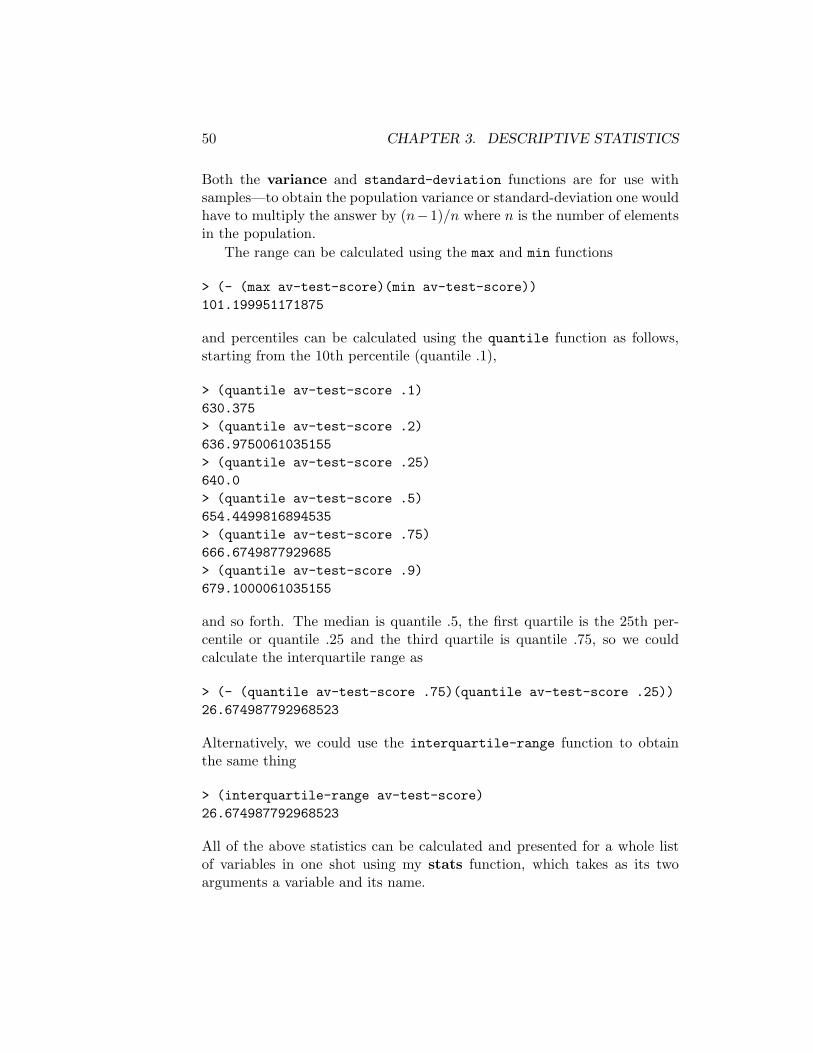
50 CHAPTER 3. DESCRIPTIVE STATISTICS
Both the variance and standard-deviation functions are for use withsamples—to obtain the population variance or standard-deviation one wouldhave to multiply the answer by (n−1)/n where n is the number of elementsin the population.
The range can be calculated using the max and min functions
> (- (max av-test-score)(min av-test-score))101.199951171875
and percentiles can be calculated using the quantile function as follows,starting from the 10th percentile (quantile .1),
> (quantile av-test-score .1)630.375> (quantile av-test-score .2)636.9750061035155> (quantile av-test-score .25)640.0> (quantile av-test-score .5)654.4499816894535> (quantile av-test-score .75)666.6749877929685> (quantile av-test-score .9)679.1000061035155
and so forth. The median is quantile .5, the first quartile is the 25th per-centile or quantile .25 and the third quartile is quantile .75, so we couldcalculate the interquartile range as
> (- (quantile av-test-score .75)(quantile av-test-score .25))26.674987792968523
Alternatively, we could use the interquartile-range function to obtainthe same thing
> (interquartile-range av-test-score)26.674987792968523
All of the above statistics can be calculated and presented for a whole listof variables in one shot using my stats function, which takes as its twoarguments a variable and its name.
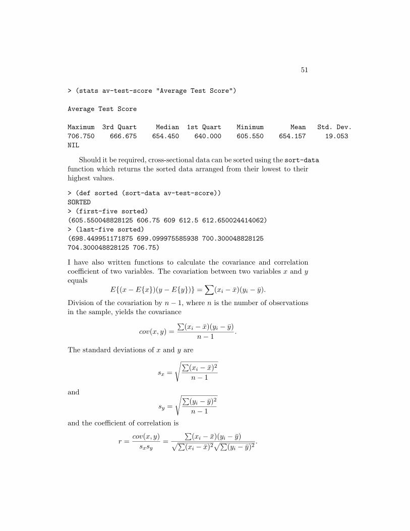
51
> (stats av-test-score "Average Test Score")
Average Test Score
Maximum 3rd Quart Median 1st Quart Minimum Mean Std. Dev.706.750 666.675 654.450 640.000 605.550 654.157 19.053NIL
Should it be required, cross-sectional data can be sorted using the sort-datafunction which returns the sorted data arranged from their lowest to theirhighest values.
> (def sorted (sort-data av-test-score))SORTED> (first-five sorted)(605.550048828125 606.75 609 612.5 612.650024414062)> (last-five sorted)(698.449951171875 699.099975585938 700.300048828125704.300048828125 706.75)
I have also written functions to calculate the covariance and correlationcoefficient of two variables. The covariation between two variables x and yequals
E(x− Ex)(y − Ey) =∑
(xi − x)(yi − y).
Division of the covariation by n− 1, where n is the number of observationsin the sample, yields the covariance
cov(x, y) =∑
(xi − x)(yi − y)n− 1
.
The standard deviations of x and y are
sx =
√∑(xi − x)2
n− 1
and
sy =
√∑(yi − y)2
n− 1
and the coefficient of correlation is
r =cov(x, y)
sxsy=
∑(xi − x)(yi − y)√∑
(xi − x)2√∑
(yi − y)2.

52 CHAPTER 3. DESCRIPTIVE STATISTICS
The covariance and correlation functions can be demonstrated using theCalifornia district reading and math test scores, the average of which pro-duced the average test score data used previously.
> (def math-test-score (read-data-file "calmts.dat"))MATH-TEST-SCORE> (def read-test-score (read-data-file "calrts.dat"))READ-TEST-SCORE> (covariance math-test-score read-test-score)348.0346025684739> (correlation math-test-score read-test-score)0.9229014922799678
The characteristics of cross-section data can be observed very easily usingthe boxplot.
> (boxplot av-test-score)#<Object: 81c6358, prototype = SCATTERPLOT-PROTO>
It turns out that XLispStat creates an object represented by the window inwhich the boxplot appears and the line returned by the Interpreter can beused to identify the window containing the plot at a later stage, although thisis a feature we will not be making use of. The top of the box represents theupper quartile and the bottom represents the lower quartile. The horizontalline through the middle of the box denotes the median. The upper whiskergives the maximum value and the lower whisker gives the minimum value.The plot is shown in Figure 1.
An alternative way of looking at cross-sectional data is to plot them ina histogram. XLispStat has a histogram function that also generates anobject in memory. A histogram of the average test score data is generatedbelow and is shown in Figure 2. For future use we give the object a name.
> (def histplot (histogram av-test-score))HISTPLOT
Histogram plots can be used as a sneaky way of obtaining a frequency dis-tribution. We can send HISTPLOT, which is stored as an object in memory,a message asking it for the counts in the bins as follows.
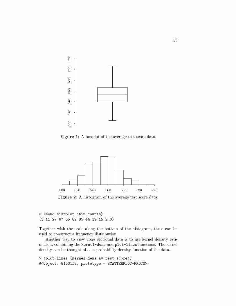
53
Figure 1: A boxplot of the average test score data.
Figure 2: A histogram of the average test score data.
> (send histplot :bin-counts)(3 11 27 67 65 82 85 44 19 15 2 0)
Together with the scale along the bottom of the histogram, these can beused to construct a frequency distribution.
Another way to view cross sectional data is to use kernel density esti-mation, combining the kernel-dens and plot-lines functions. The kerneldensity can be thought of as a probability density function of the data.
> (plot-lines (kernel-dens av-test-score))#<Object: 81531f8, prototype = SCATTERPLOT-PROTO>

54 CHAPTER 3. DESCRIPTIVE STATISTICS
As in the case of the other plotting functions the plot-lines function cre-ates an object in memory. The resulting kernel density is shown in Figure 3.
Figure 3: A kernel-density plot of the average test score data.
The relation between two variables can be visualized using the functionplot-points which, like the other plotting functions, creates an object inmemory.
> (def xyplot (plot-points math-test-score read-test-score))XYPLOT> (send xyplot :variable-label 0 "math test score")"math test score"> (send xyplot :variable-label 1 "reading test score")"reading test score"
The resulting plot is shown in Figure 4. Notice the messages sent to theobject xyplot to label the axes.
Time-series data present a special problem in that they must be orderedaccording to date. Accordingly, to meaningfully work with these data wemust insure that each series has a corresponding dates-list that conformsto it. Appropriate dates can be added in the spreadsheet program beforesaving the data as a matrix to read into XLispStat. The dates must berepresented as a column of real numbers. And, as noted in the previouschapter, my setdates function can be used to create a date-list for a series

55
Figure 4: A scatter plot of the math and reading test scores.
that does not yet have one and my date2obs function can be used to findthe observation number (starting at 0) associated with any given date in thedatelist conforming to a particular time series of interest.
Time-series can be plotted using the following commands, which we il-lustrate using the data set contained in the file cpism.lsp created in theprevious chapter.
> (def plotdates (- dates-cpim 1900))PLOTDATES> (def tsplot (plot-lines plotdates cpius))TSPLOT> (send tsplot :add-lines plotdates cpica)NIL> (send tsplot :add-points plotdates cpius)NIL> (send tsplot :variable-label 1 "Index: 1995 = 100")"Index: 1995 = 100"
In order for avoid the dates being in scientific notation along the bottomof the plot, it is necessary to shorten the individual dates by subtracting1900 from the date list. We next create the plot using the plot-linesfunction to plot the U.S. CPI, then send it an :add-lines message to plot

56 CHAPTER 3. DESCRIPTIVE STATISTICS
the Canadian CPI and then an add-points message to impose points on theU.S. series to distinguish it from the Canadian one. After a label is addedto the vertical axis, the plot is saved as Figure 5, with the description atthe bottom indicating that the thick line is the U.S. CPI and the thin lineis the Canadian CPI. Because the dates do not print properly, XLispStattime series plots are not of publishable quality—to obtain publishable plots,we simply write a matrix consisting of the date-list and the variables to beplotted to a file and create a encapsulated post-script file using Gnuplot.
Figure 5: Consumer price indexes: U.S. (thick line) andCanada (thin line).
It is freqently desirable to take the first-difference of a time series. Wecan do this using the difference function. The first differences of thelogarithms of the Canadian and U.S. CPI series, multiplied by 100, give thecountries’ month-to-month inflation rates.
> (def infmca (* 100 (difference (log cpim-canada))))INFMCA> (def infmus (* 100 (difference (log cpim-us))))INFMUS> (def dates-infm (remove-first-element dates-cpim))DATES-INFM

57
Notice that we must also create a new shorter datelist to conform to thenew month-to-month inflation series.
It is also useful to calculate the year-over-year inflation rate. As notedearlier, this requires that we create 12 period lagged CPI series by droppingthe last 12 observations and then shorten the unlagged series by droppingthe first 12 observations.
> (def cpimus-12 (remove-last 12 cpim-us))CPIMUS-12> (def cpimca-12 (remove-last 12 cpim-canada))CPIMCA-12> (def cpimus (remove-first 12 cpim-us))CPIMUS> (def cpimca (remove-first 12 cpim-canada))CPIMCA> (def infyus (* 100 (- (log cpimus)(log cpimus-12))))INFYUS> (def infyca (* 100 (- (log cpimca)(log cpimca-12))))INFYCA> (def dates-infy (remove-first 12 cpim-dates))DATES-INFY
Let us now use Gnuplot to create publication quality time series graphsof these U.S. and Canadian inflation rates. First we write the month-to-month and year-to-year inflation rates, along with their date lists to matrixfiles.
> (write-matrix-to-file (bind-columns dates-infm infmus infmca)"infm.mat")
T> (write-matrix-to-file (bind-columns dates-infy infyus infyca)"infy.mat")
T
Then we modify the file plottser.plt, contained in xlispdf.exe andxlispdf.tar.gz, to yield the following.2
2The approach adopted here is more sophisticated but much simpler than that in mylittle Gnuplot mini-manual that can be obtained off my web-page.
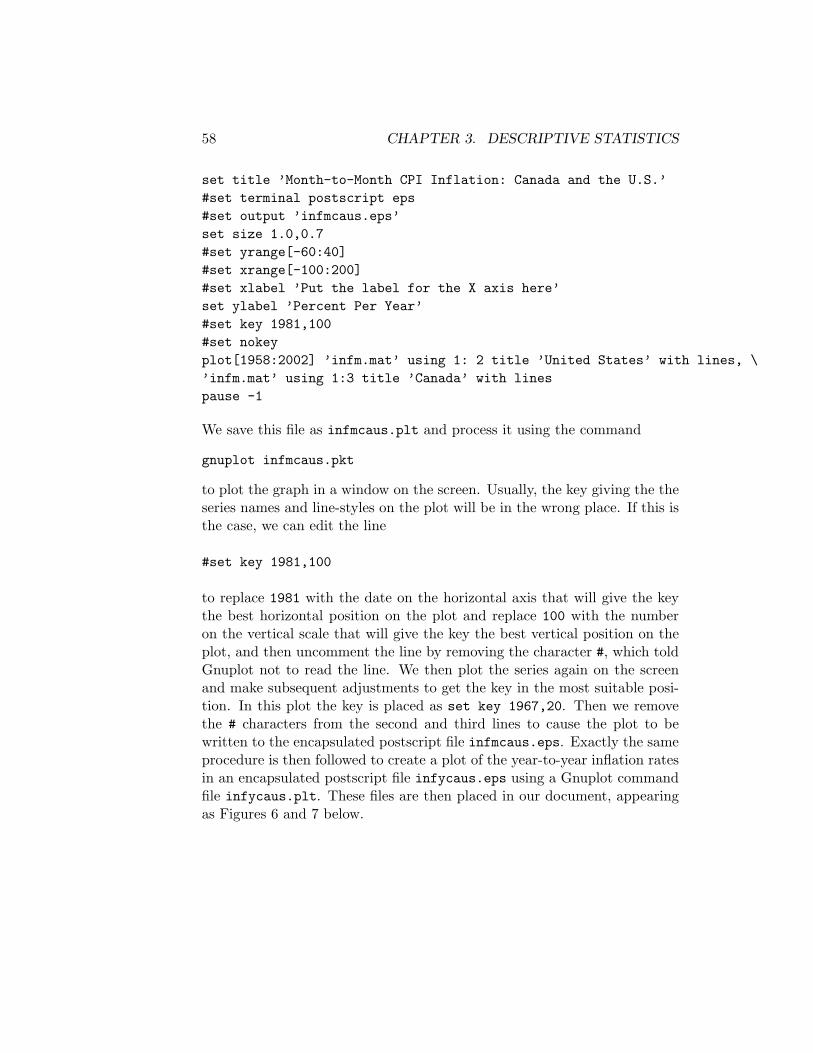
58 CHAPTER 3. DESCRIPTIVE STATISTICS
set title ’Month-to-Month CPI Inflation: Canada and the U.S.’#set terminal postscript eps#set output ’infmcaus.eps’set size 1.0,0.7#set yrange[-60:40]#set xrange[-100:200]#set xlabel ’Put the label for the X axis here’set ylabel ’Percent Per Year’#set key 1981,100#set nokeyplot[1958:2002] ’infm.mat’ using 1: 2 title ’United States’ with lines, \’infm.mat’ using 1:3 title ’Canada’ with linespause -1
We save this file as infmcaus.plt and process it using the command
gnuplot infmcaus.pkt
to plot the graph in a window on the screen. Usually, the key giving the theseries names and line-styles on the plot will be in the wrong place. If this isthe case, we can edit the line
#set key 1981,100
to replace 1981 with the date on the horizontal axis that will give the keythe best horizontal position on the plot and replace 100 with the numberon the vertical scale that will give the key the best vertical position on theplot, and then uncomment the line by removing the character #, which toldGnuplot not to read the line. We then plot the series again on the screenand make subsequent adjustments to get the key in the most suitable posi-tion. In this plot the key is placed as set key 1967,20. Then we removethe # characters from the second and third lines to cause the plot to bewritten to the encapsulated postscript file infmcaus.eps. Exactly the sameprocedure is then followed to create a plot of the year-to-year inflation ratesin an encapsulated postscript file infycaus.eps using a Gnuplot commandfile infycaus.plt. These files are then placed in our document, appearingas Figures 6 and 7 below.

59
-15
-10
-5
0
5
10
15
20
25
30
35
1960 1965 1970 1975 1980 1985 1990 1995 2000
Per
cent
Per
Yea
r
United StatesCanada
Figure 6: Month-to-month CPI inflation rates: United States and Canada.
-2
0
2
4
6
8
10
12
14
1960 1965 1970 1975 1980 1985 1990 1995 2000
Per
cent
Per
Yea
r
United StatesCanada
Figure 7: Year-to-year CPI inflation rates: United States and Canada.
I have written two additional functions that are useful in examining timeseries data. They are the standard autocorrelation and partial autocorrela-tion functions, acf and pacf. They are applied to the Canadian CPI andCPI-inflation rate series as follows, where UCL and LCL refer to the upperand lower confidence limits.3
3Readers whose understanding of the time-series concepts underlying these functionsshould read my “Note on Time-Series Basics”, available at the same site as my StatisticsFor Economists: A Beginning.
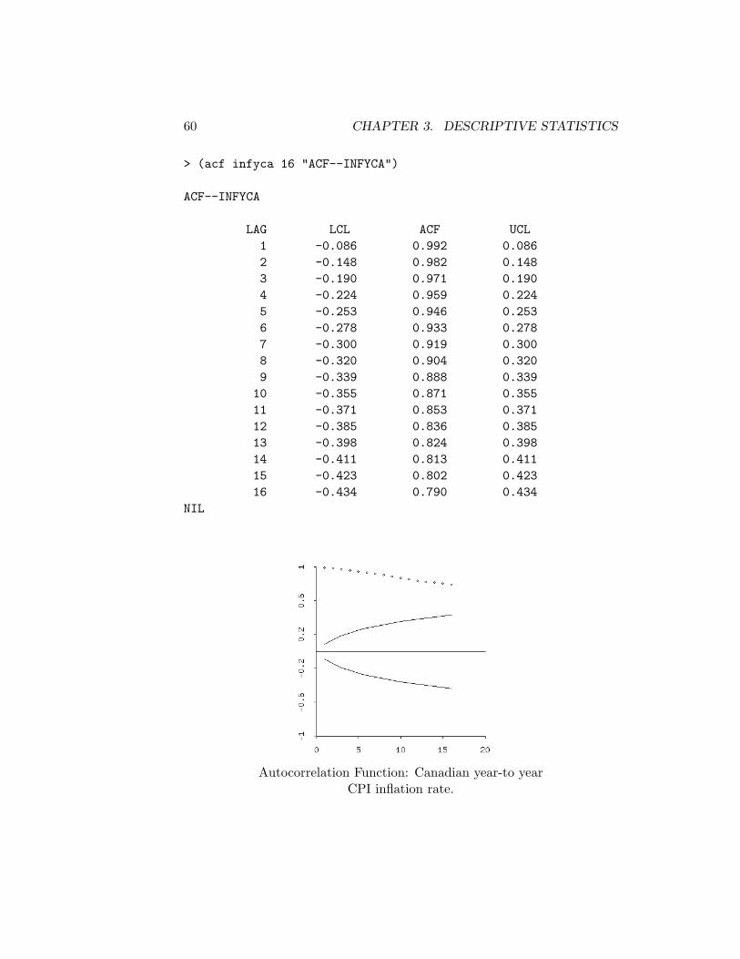
60 CHAPTER 3. DESCRIPTIVE STATISTICS
> (acf infyca 16 "ACF--INFYCA")
ACF--INFYCA
LAG LCL ACF UCL1 -0.086 0.992 0.0862 -0.148 0.982 0.1483 -0.190 0.971 0.1904 -0.224 0.959 0.2245 -0.253 0.946 0.2536 -0.278 0.933 0.2787 -0.300 0.919 0.3008 -0.320 0.904 0.3209 -0.339 0.888 0.33910 -0.355 0.871 0.35511 -0.371 0.853 0.37112 -0.385 0.836 0.38513 -0.398 0.824 0.39814 -0.411 0.813 0.41115 -0.423 0.802 0.42316 -0.434 0.790 0.434
NIL
Autocorrelation Function: Canadian year-to yearCPI inflation rate.
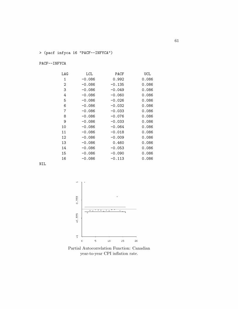
61
> (pacf infyca 16 "PACF--INFYCA")
PACF--INFYCA
LAG LCL PACF UCL1 -0.086 0.992 0.0862 -0.086 -0.135 0.0863 -0.086 -0.049 0.0864 -0.086 -0.060 0.0865 -0.086 -0.026 0.0866 -0.086 -0.032 0.0867 -0.086 -0.033 0.0868 -0.086 -0.076 0.0869 -0.086 -0.033 0.086
10 -0.086 -0.064 0.08611 -0.086 -0.018 0.08612 -0.086 -0.009 0.08613 -0.086 0.460 0.08614 -0.086 -0.053 0.08615 -0.086 -0.090 0.08616 -0.086 -0.113 0.086
NIL
Partial Autocorrelation Function: Canadianyear-to-year CPI inflation rate.
62 CHAPTER 3. DESCRIPTIVE STATISTICS
The autocorrelations portrayed in the corresponding table and plot arethe simple correlations between the current level of the variable and each ofthe 16 past levels in turn. The partial autocorrelations are the correlationsbetween the current level of the variable and each of the 16 past levels holdingthe remaining 15 lagged levels constant. From an examination of the plotof the autocorrelations, one cannot rule out the possibility that the secondlag of the variable is correlated with is current level simply because it iscorrelated with the first lag which is correlated with the current level. As canbe clearly seen from the plot of the partial autocorrelations, the current leveland one lag are highly correlated, but the current level and most subsequentlags are completely uncorrelated once the correlation between the currentlevel and first lag is accounted for.

Chapter 4
Hypothesis Tests
This chapter is devoted to issues surrounding the testing of hypothesis.Readers needing background should read Chapter 2 of the Stock and Watsontextbook,1 or for a more elementary treatment, Chapters 2 through 7 of myelementary statistics notes cited at the beginning of the previous chapter.2
4.1 Probability Densities and Quantiles
XLispStat can be used, of course, to calculate probability densities andquantiles of the commonly used probability distributions. Take first thestandard-normal distribution. We use the normal-cdf function to cal-culate the fraction of the cumulative probability density lying to the left ofsome selected quantile z.
> (normal-cdf -3)0.00135> (normal-cdf -2)0.02275> (normal-cdf -1)0.15865> (normal-cdf 0)0.5> (normal-cdf 1)0.84134
1James H. Stock and Mark W. Watson, Introduction to Econometrics2Statistics for Economists: A Beginning.
63
64 CHAPTER 4. HYPOTHESIS TESTS
> (normal-cdf 2)0.97725> (normal-cdf 3)0.99865
Using calculations like these we can confirm that
> (* (normal-cdf -1) 2)0.31731> (* (normal-cdf -2) 2)0.04550
or nearly 32 percent of the distribution lies outside one standard deviationfrom the mean and somewhat less than 5 percent of the distribution liesoutside two standard deviations. It follows that about 68 percent of thedistribution lies within one standard deviation from the mean and somewhatmore than 95 percent of it lies within two standard deviations from the mean.
We can also find the z-value or quantile associated with any cumulativeprobability or quantile using the normal-quant function.
> (normal-quant .95)1.6446> (normal-quant .975)1.95996
confirms that approximately 1.645 is the critical value of z to the left ofwhich 95 percent of the density lies, and to the right of which 5 percent ofthe density lies, and approximately 1.96 is the z-value to the left of which.975 of the distribution lies and to the right of which only .025 or 2.5 percentof the density lies. And the z-value beyond which only 1 percent of thedistribution lies is
> (normal-quant .99)2.32635
Now consider the t-distribution. Both the t-cdf and t-quant func-tions take two arguments—first the quantile or cumulative density and sec-ond the degrees of freedom. With 5 degrees of freedom, the percentage ofthe probability density falling to the left of +2 and +1 standard deviations,respectively, are
> (t-cdf 2 5)0.94903
4.1. PROBABILITY DENSITIES AND QUANTILES 65
> (t-cdf 1 5)0.81839
Note that the above cumulative densities are smaller than would be obtainedusing (normal-cdf 2) and (normal-cdf 1) because the t-distribution hasflatter tails. The t-value or quantile to the left of which 95 percent of thedensity lies can be calculated as
> (t-quant .95 3)2.35336
which is more standard deviations from the mean than the 95th quantile ofthe normal distribution. Here we used only 3 degrees of freedom.
Turn now to the binomial distribution, the cumulative densities ofwhich are obtained using the binomial-cdf function which takes threearguments—in order, the number of occurrences, the number of tries andthe probability of a success. Thus, the probability of getting 6 or less headsin 10 flips of a fair coin is
> (binomial-cdf 6 10 .5)0.828125
And the probability of getting 5 or less heads in 10 tosses is
> (binomial-cdf 5 10 .5)0.623047
So the probability of obtaining 6 heads in 10 tosses is
> (- (binomial-cdf 6 10 .5)(binomial-cdf 5 10 .5))0.205078
and the probability of getting 5 heads in 10 tosses is
> (- (binomial-cdf 5 10 .5)(binomial-cdf 4 10 .5))0.246094
When the probability of success is .5 the binomial distribution is symmetri-cal, so the probability of obtaining 4 heads in 10 tosses
> (- (binomial-cdf 4 10 .5)(binomial-cdf 3 10 .5))0.205078
is the same as the probability of obtaining 6 heads in 10 tosses. In this casethe probability of obtaining either 0 heads or 10 heads in 10 tosses is thusequal to

66 CHAPTER 4. HYPOTHESIS TESTS
> (- (binomial-cdf 10 10 .5)(binomial-cdf 9 10 .5))9.765625E-4
or .0009765625.
Next consider the poisson distribution. Suppose that the f-word is heard3 times per minute on average on the front steps of a particular high-school.Using the poisson-cdf function we can calculate the probability that it willbe heard twice or less in a given minute as
> (poisson-cdf 2 3)0.423190
and the probability it would be said three times or less would be
> (poisson-cdf 3 3)0.647232
so the probability it would be said three times is
> (- (poisson-cdf 3 3)(poisson-cdf 2 3))0.224042
Here, the left-most argument in the poisson-cdf function is the specifiednumber of occurrences and the other argument is the mean number of oc-currences.
Turning now to the F-distribution, suppose we have a value of theF-statistic of 3.07 with 3 degrees of freedom in the numerator and 7 in thedenominator. The probability of obtaining a value of the statistic less than3.07 is obtained using the f-cdf function as
> (f-cdf 3.07 3 7)0.899755
or approximately .9 and the probability of obtaining a larger value is thusapproximately equal to .1. The 10% critical value of F can be obtained fromthe f-quant function as follows.
> (f-quant .9 3 7)3.074072
Notice that unity minus the chosen critical probability is entered in thef-quant function in the left-most position, followed by the degrees of free-dom in the numerator and denominator respectively. Appropriately modi-fied versions of the last expression above can thus be passed to the Inter-preter to obtain any chosen critical value of F.

4.1. PROBABILITY DENSITIES AND QUANTILES 67
The critical values of the chi-square distribution can be found using thechisq-quant function.
> (chisq-quant .95 10)18.307038
where, as in the case of the F-distribution, the left-most number (.95) isunity minus the chosen critical probability, and the right-most number isthe degrees of freedom. The probability that a Chi-square statistic willbe below some particular level—say, 10.52—when there are 25 degrees offreedom is obtained using the chisq-cdf function.
> (chisq-cdf 10.52 25)0.005001
This gives the mass in (or area of) the lower tail of the distribution below10.52. This area is small because the mean of the distribution, which equalsthe degrees of freedom, is 25. Consider, alternatively, the probability thatthe statistic will be below some value above the mean, say 50.
> (chisq-cdf 50 25)0.997869
The probability mass in the corresponding upper tail is
> (- 1 (chisq-cdf 50 25))0.003131
A distribution of interest for which XLispStat does not have cumula-tive density and quantile functions is the exponential distribution. Thisdistribution applies to the amount of time between occurrences. The prob-ability that the waiting time X will be above some number x is
P (X ≥ x) = e−λx
where λ is the reciprocal of the mean waiting time. We can calculate thisprobability using XLispStat as follows when the mean waiting time is 4hours (λ = .25) and x is 6 hours:
> (exp (* -.25 6))0.223130
The probability of having to wait longer than the mean will be
> (exp (* -.25 4))0.367879
68 CHAPTER 4. HYPOTHESIS TESTS
4.2 Plotting Probability Distributions
To plot probability distributions we need the probability densities ratherthan the cumulative probability densities. And we need a range of valuesfor which the densities are to be plotted.
It is often useful to compare kernel densities with the normal distributionto make a guess as to whether a particular variable is in fact normallydistributed. Consider, for example, the kernel-density of the average testscore plotted in Figure 3. To compare it to a normal distribution we needto standardise the variable. Taking the deviation of the average test scoresfrom their mean and dividing by the standard deviation of the average testscore, we create the new variable z-ats.
> (def z-ats (/ (- av-test-score (mean av-test-score))(standard-deviation av-test-score)))Z-ATS
Next, we calculate the kernel-density of this new standardised average-test-score variable.
> (def kd-ats (kernel-dens z-ats))KD-ATS
The kernel-dens function produces a list-object containing two lists—alist of 30 evenly-spaced levels of the standardised average test score runningfrom minimum to maximum with zero in the middle (representing the x-axisin a kernel-density plot), and a list giving the density of the kernel at each ofthese average test scores. The former list can be obtained from the kd-atsobject using the select function.
> (def zval (select kd-ats 0))ZVAL
A plot object kdplot is created
> (def kdplot (plot-lines kd-ats))KDPLOT
and then sent an add-lines message to add a standard normal densityfunction.
> (send kdplot :add-lines zval (normal-dens zval))NIL

4.2. PLOTTING PROBABILITY DISTRIBUTIONS 69
The result is shown in Figure 8—the approximation is obviously poor towardthe center of the kernel.3
Figure 8: Standardized kernel-density of average test scorescompared with normal-density.
To enable one to visualize the shapes of the various distributions fordifferent values of their parameters, I have constructed a number of demo-plot functions. These will load automatically with addfuncs.lsp and thecode for them can be examined by loading that file into an editor. Thesefunctions are as follows: plot-binomial
> (plot-binomial n p)
takes the two parameters n and p, where n is the number of tries and p is theprobability of success. These can be chosen at will for illustrating variousshapes of the distribution.
3Actually, four types of kernels are supported. In Figure 8 the default, B
(bisquare), is used. The others are G (Gaussian), T (triangular) and U (uniform).To use, say, the Gaussian kernel we would rewrite the expression defining z-ats as(def kd-ats (kernel-dens z-ats :type ’g)).
70 CHAPTER 4. HYPOTHESIS TESTS
plot-poisson
> (plot-poisson r m)
plots the Poisson distribution using the two parameters r and m, where ris the right-most point in the range along which the distribution is to beplotted (the left-most point is, of course, zero) and m is the mean.
plot-chisq
> (plot-chisq v)
plots the Chi-square distribution for a chosen degrees of freedom parameterv.
plot-F
> (plot-F r dfn dfd)
plots the F-distribution, where r is the right-most point of the range ofpositive values over which the function is to be plotted and dfn and dfdrepresent the degrees of freedom in the numerator and denominator.
plot-t
> (plot-t v)
plots the t-distribution using the one parameter v representing the degreesof freedom.
plot-standard-normal
> (plot-standard-normal)
plots the standard normal distribution—the function takes no parameters.
plot-t-on-normal
> (plot-t-on-normal v)
plots a t-distribution with chosen degrees of freedom v on top of a standardnormal distribution that has already been plotted using the plot-standard-normal function. Successive application of this function will enable you tovisualise how the t-distribution approaches the standard normal distributionas the degrees of freedom increase.
plot-normal-on-t
> (plot-normal-on-t)
plots a standard normal distribution on top of a t-distribution that has beenpreviously plotted using the plot-t function. No parameters are required.

4.3. GENERATING RANDOM DATA 71
4.3 Generating Random Data
We can generate a set (list) of independent random numbers distributeduniformly between zero and 1 using the function
> (def nums (uniform-rand 2000))NUMS
This generates 2000 numbers. By multiplying every number in the list byan appropriate constant n we can transform the list into a list of randomnumbers uniformly distributed between 0 and n. Letting n = 5 we have
> (def newnums (* nums 5))NEWNUMS
To convince ourselves that the distribution of these numbers could havereasonably come from a uniform distribution between 0 and 5 we plot itskernel-density in Figure 9.
> (plot-lines (kernel-dens newnums))#<Object: 81a23e8, prototype = SCATTERPLOT-PROTO>
The list can be transformed to shift the range to, say, between 1 and 6 byadding 1 to each element in it.
To select a sample of, say 10, random integers between 2 and 50 we sendthe Interpreter the expression
> (def sampnums (sample (iseq 2 50) 10))SAMPNUMS> sampnums(24 15 10 37 13 21 42 31 35 36)
The sampling is without replacement—no number can be selected twice.To select a sample with replacement, we send the following message to theInterpreter, placing a t in position after the number specifying the size ofsample.
> (sample (iseq 2 4) 10 t)(2 4 3 2 4 3 2 3 3 3)
To draw a sample of 100 from a standard normal distribution we send themessage
> (def normvars (normal-rand 100)))NORMVARS

72 CHAPTER 4. HYPOTHESIS TESTS
Figure 9: Kernel-density of uniformily distributed randomnumbers between 0 and 5.
We could make this sample come from a normal distribution with meanµ = 10 and standard deviation σ = 3 by simply transforming NORMVARS,multiplying each of the numbers in that list by the standard deviation andadding the mean—this simply transforms a z-value into an x-value where zis the standardised value of x.
> (def newnormvars (+ (* normvars 3) 10))NEWNORMVARS
To select a list of three samples of 100 from the standard normal distributionwe execute the command
> (def normlist (normal-rand (list 100 100 100)))NORMLIST
Similarly, to select samples of 10 from a t- Chi-square or F-distribution, usethe commands
> (def tnums (t-rand 10 4))TNUMS> (def csnums (chisq-rand 10 4))CSNUMS
4.4. TESTS OF THE MEAN AND STANDARD DEVIATION 73
> (def fnums (f-rand 10 2 5))FNUMS
choosing degrees of freedom equal to 4 in the case of the t- and Chi-squaredistributions and 2 degrees of freedom in the numerator and 5 degrees offreedom in the denominator in the case of the F-distribution.
4.4 Tests of the Mean and Standard Deviation
Suppose that we are interested in whether the mean California district av-erage test score exceeds 650. Our null-hypothesis then becomes µ = 650,the alternative hypothesis is µ > 650, and our point estimate of µ is X, thesample mean. We need to calculate the mean of the average test scores, thesample size and the sample standard deviation.
> (def av-test-score (read-data-file "calats.dat"))AV-TEST-SCORE> (def meanats (mean av-test-score))MEANATS> meanats654.1565480550131> (def n (length av-test-score))N> n420> (def stdats (standard-deviation av-test-score))STDATS> stdats19.05334764361879
Since the variance of the mean is
σ2m =
σ2
n
we calculate a point estimate of the standard deviation of the mean usingthe sample standard deviation and the sample size as follows,
> (def std-meanats (/ stdats (sqrt n)))STD-MEANATS> std-meanats0.929708167766067
74 CHAPTER 4. HYPOTHESIS TESTS
The t-value is then
> (def trat (/ (- meanats 650) std-meanats))TRAT> trat4.470809442279713
and the P-Value of the test, which here gives the probability that samplemean could be greater than its observed value if the null-hypothesis is true,is
> (def pv (- 1 (normal-cdf trat)))PV> pv.000003896205348130621
so we can reject the null-hypothesis at the 1% level. A 1% confidence intervalfor the population mean of the average test score data, µ, can be calculatedas follows, starting with the half-width for the confidence interval.
> (def hw (* std-meanats (normal-quant .99)))HW> hw2.162824619560995> (def lci (- meanats hw))LCI> (def uci (+ meanats hw))UCI> lci651.9937234354521> uci656.3193726745741
so that 651.99 < µ < 656.32.Now let us test the hypothesis that the standard deviation of the pop-
ulation is equal to σ0 = 20. The sum of squares of n − 1 standardisedindependent normal variates is distributed as Chi-Square with n−1 degreesof freedom. That is
n∑
i=1
Z 2i =
n∑
i=1
(Xi − X) 2
σ2= χ 2 (n− 1)
4.5. TESTS OF THE DIFFERENCE BETWEEN TWO MEANS 75
where σ2 is the population variance and the use of X instead of µ in thecalculation reduces the number of independent summed squares, the degreesof freedom, by 1. Combining this with the formula for the sample variance,
s 2 =n∑
i=1
(Xi − X) 2
n− 1
we obtain(n− 1) s 2
σ2= χ 2 (n− 1).
Substituting σ20 = 20 2 = 400 and s 2 = stdats2 = 19.05334764361879 2 into
this expression yields
> (def chsqvar (* (- n 1)(/ (variance av-test-score) 400)))CHSQVAR> chsqvar380.2739841089518> (def pv (- 1 (chisq-cdf chsqvar (- n 1))))PV> pv0.9127908699966177
There is almost a 92% chance that the observed sample value of s of around19.05 could occur by random chance if the true value of σ were 20. Thenull-hypothesis cannot be rejected. It should be kept in mind that theformulae on which this conclusion is based incorporate an assumption thatthe average test scores are normally distributed. We will rigorously examinethis assumption below.
4.5 Tests of the Difference Between Two Means
Now let us turn to hypotheses about the difference in means. Consider, forexample, the mean rates of year-over-year CPI inflation in Canada and theUnited States. The data are in the file infcaus.lsp.
> (load "infcaus.lsp"); loading infcaus.lspT> (variables)(DATES-INF INFMMCA INFMMUS INFYYCA INFYYUS)

76 CHAPTER 4. HYPOTHESIS TESTS
The means are
> (mean infyyca)4.248020425852652> (mean infyyus)4.124029449387656
and the Canadian mean inflation rate is larger than the U.S. one by
> (def difmeans (- (mean infyyca)(mean infyyus)))DIFMEANS> difmeans0.12399097646499602
As a factual matter it is unquestionable that the year-over-year inflationrate was higher in Canada than in the U.S. over the period 1958 through2002.
Can we infer from this that the economic and political realities in Canadaas compared to the U.S. are such that there is a greater tendency for inflationto occur in the former country? This is a question about the differencesbetween the underlying process of inflation generation in the two countries,of which the data for the years 1958-2002 represent a sample. It focuseson the underlying population mean rather than the sample mean. Whatcan we infer about the difference between the population means from thedifference in the sample means? Let the null-hypothesis be that the politicaland governmental process in Canada generates the same rate of year-over-year inflation as the corresponding process in the U.S. Can we reject thisnull-hypothesis?
The difference between the sample means is a point estimate of thedifference between the population means—that is,
Eµca − µus = Xca − Xus
where Xca and Xus represent the year-over-year inflation rates of the twocountries. The variance of the difference in the sample means, where thesample means are independently distributed, is
s2dm =
s2ca
n+
s2us
n
where s2ca and s2
us are the variances of the two countries’ year-over-yearinflation rates and n is the number of months in the sample. We can thuscalculate the standard deviation of the difference in the sample means asfollows.
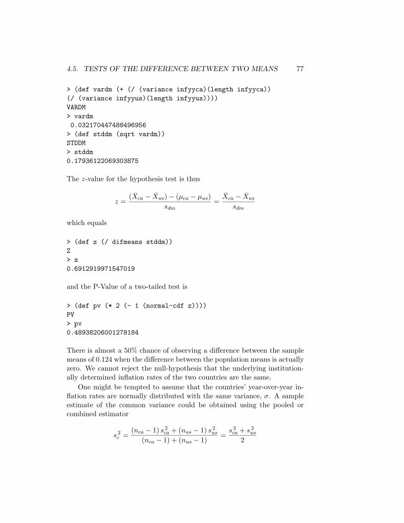
4.5. TESTS OF THE DIFFERENCE BETWEEN TWO MEANS 77
> (def vardm (+ (/ (variance infyyca)(length infyyca))(/ (variance infyyus)(length infyyus))))VARDM> vardm0.032170447488496956
> (def stddm (sqrt vardm))STDDM> stddm0.17936122069303875
The z-value for the hypothesis test is thus
z =(Xca − Xus)− (µca − µus)
sdm=
Xca − Xus
sdm
which equals
> (def z (/ difmeans stddm))Z> z0.6912919971547019
and the P-Value of a two-tailed test is
> (def pv (* 2 (- 1 (normal-cdf z))))PV> pv0.48938206001278184
There is almost a 50% chance of observing a difference between the samplemeans of 0.124 when the difference between the population means is actuallyzero. We cannot reject the null-hypothesis that the underlying institution-ally determined inflation rates of the two countries are the same.
One might be tempted to assume that the countries’ year-over-year in-flation rates are normally distributed with the same variance, σ. A sampleestimate of the common variance could be obtained using the pooled orcombined estimator
s 2c =
(nca − 1) s 2ca + (nus − 1) s 2
us
(nca − 1) + (nus − 1)=
s 2ca + s 2
us
2

78 CHAPTER 4. HYPOTHESIS TESTS
where the sample sizes are the same for both countries.4 The variance ofthe difference in the means would then become
s 2Xca − Xus = s 2c
[1
nca+
1nus
]=
2 s 2c
n=
s 2ca + s 2
us
n
where ncs = nus = n. Before going this route, however, we should plotthe year-over-year inflation rate series to see if they could reasonably beregarded as normally distributed.
> (def infplot (plot-lines (kernel-dens infyyus)))INFPLOT> (send infplot :add-lines (kernel-dens infyyca))NIL> (send infplot :add-points (kernel-dens infyyus))NIL
It is obvious from the presentation of this plot in Figure 10 that normalitycan be rejected.
Figure 10: Kernel-densities of the U.S. and Canadian year-over-yearinflation rates.
4Essentially, we are taking weighted average of the two variances with the weights beingthe countries’ (in this case equal) contributions to the total degrees of freedom.
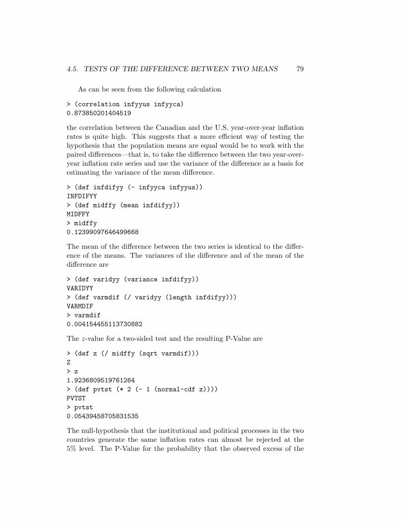
4.5. TESTS OF THE DIFFERENCE BETWEEN TWO MEANS 79
As can be seen from the following calculation
> (correlation infyyus infyyca)0.873850201404519
the correlation between the Canadian and the U.S. year-over-year inflationrates is quite high. This suggests that a more efficient way of testing thehypothesis that the population means are equal would be to work with thepaired differences—that is, to take the difference between the two year-over-year inflation rate series and use the variance of the difference as a basis forestimating the variance of the mean difference.
> (def infdifyy (- infyyca infyyus))INFDIFYY> (def midffy (mean infdifyy))MIDFFY> midffy0.12399097646499668
The mean of the difference between the two series is identical to the differ-ence of the means. The variances of the difference and of the mean of thedifference are
> (def varidyy (variance infdifyy))VARIDYY> (def varmdif (/ varidyy (length infdifyy)))VARMDIF> varmdif0.004154455113730882
The z-value for a two-sided test and the resulting P-Value are
> (def z (/ midffy (sqrt varmdif)))Z> z1.9236809519761264> (def pvtst (* 2 (- 1 (normal-cdf z))))PVTST> pvtst0.05439458705831535
The null-hypothesis that the institutional and political processes in the twocountries generate the same inflation rates can almost be rejected at the5% level. The P-Value for the probability that the observed excess of the
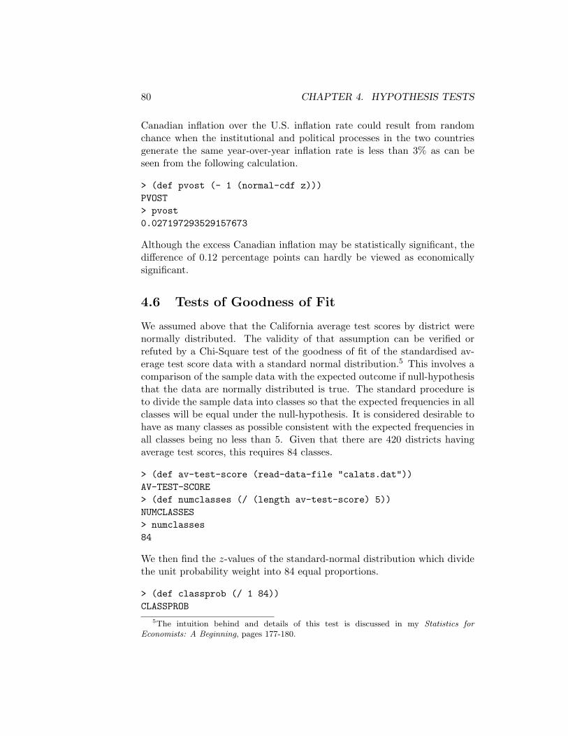
80 CHAPTER 4. HYPOTHESIS TESTS
Canadian inflation over the U.S. inflation rate could result from randomchance when the institutional and political processes in the two countriesgenerate the same year-over-year inflation rate is less than 3% as can beseen from the following calculation.
> (def pvost (- 1 (normal-cdf z)))PVOST> pvost0.027197293529157673
Although the excess Canadian inflation may be statistically significant, thedifference of 0.12 percentage points can hardly be viewed as economicallysignificant.
4.6 Tests of Goodness of Fit
We assumed above that the California average test scores by district werenormally distributed. The validity of that assumption can be verified orrefuted by a Chi-Square test of the goodness of fit of the standardised av-erage test score data with a standard normal distribution.5 This involves acomparison of the sample data with the expected outcome if null-hypothesisthat the data are normally distributed is true. The standard procedure isto divide the sample data into classes so that the expected frequencies in allclasses will be equal under the null-hypothesis. It is considered desirable tohave as many classes as possible consistent with the expected frequencies inall classes being no less than 5. Given that there are 420 districts havingaverage test scores, this requires 84 classes.
> (def av-test-score (read-data-file "calats.dat"))AV-TEST-SCORE> (def numclasses (/ (length av-test-score) 5))NUMCLASSES> numclasses84
We then find the z-values of the standard-normal distribution which dividethe unit probability weight into 84 equal proportions.
> (def classprob (/ 1 84))CLASSPROB
5The intuition behind and details of this test is discussed in my Statistics forEconomists: A Beginning, pages 177-180.

4.6. TESTS OF GOODNESS OF FIT 81
> classprob0.011904761904761904> (def ncbound (repeat 0 83))NCBOUND> (setf (select ncbound 0)(normal-quant classprob))-2.260188991329375> (dotimes (i 82)(setf (select ncbound (+ i 1))(normal-quant (* classprob (+ i 2)))))> (first-five ncbound)(-2.260188991329375 -1.9807523966472789 -1.8027430907391901-1.668391193947079 -1.5587835495029951)
> (last-five ncbound)(1.558783549502995 1.6683911939470786 1.80274309073918881.9807523966472784 2.2601889913293727)> (chosen-five ncbound 40)(-0.059717099785322886 -0.02984524291923956 0.0 0.029845242919239420.0597170997853226)
These quantiles can then be used to obtain the corresponding boundariesfor the standardised average test score data. The data are standardised asfollows.
> (def meanats (mean av-test-score))MEANATS> meanats654.1565480550131> (def stdats (standard-deviation av-test-score))STDATS> stdats19.05334764361879> (def datbound (+ (* stdats ncbound) meanats))DATBOUND> (length ncbound)83> (length datbound)83> (first-five datbound)(611.0923814629344 616.4165840457614 619.8082572350276622.3681106311872 624.4565031851785)
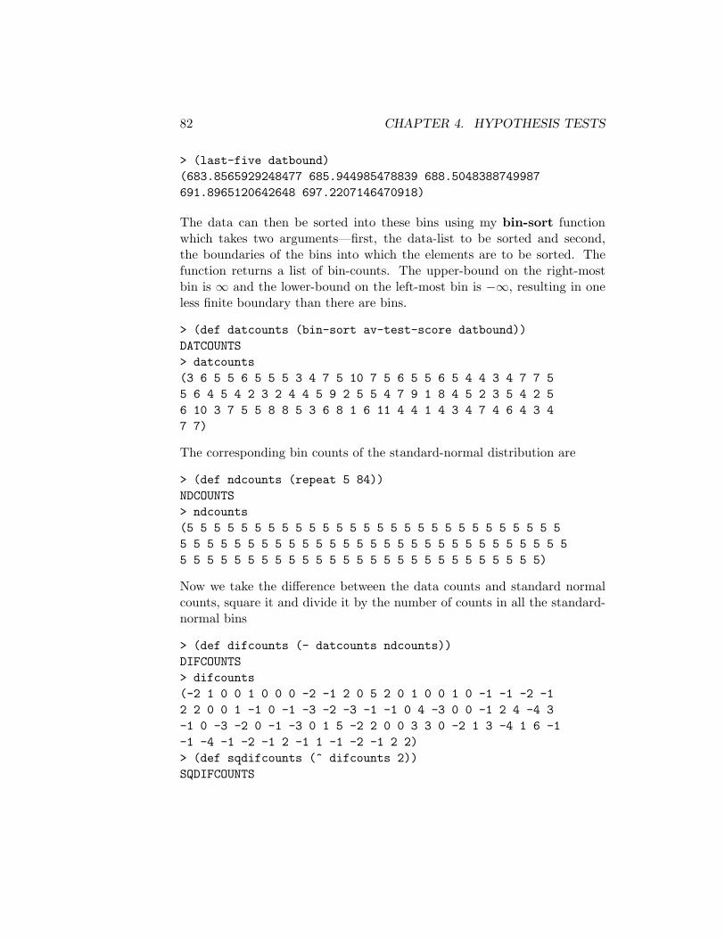
82 CHAPTER 4. HYPOTHESIS TESTS
> (last-five datbound)(683.8565929248477 685.944985478839 688.5048388749987691.8965120642648 697.2207146470918)
The data can then be sorted into these bins using my bin-sort functionwhich takes two arguments—first, the data-list to be sorted and second,the boundaries of the bins into which the elements are to be sorted. Thefunction returns a list of bin-counts. The upper-bound on the right-mostbin is ∞ and the lower-bound on the left-most bin is −∞, resulting in oneless finite boundary than there are bins.
> (def datcounts (bin-sort av-test-score datbound))DATCOUNTS> datcounts(3 6 5 5 6 5 5 5 3 4 7 5 10 7 5 6 5 5 6 5 4 4 3 4 7 7 55 6 4 5 4 2 3 2 4 4 5 9 2 5 5 4 7 9 1 8 4 5 2 3 5 4 2 56 10 3 7 5 5 8 8 5 3 6 8 1 6 11 4 4 1 4 3 4 7 4 6 4 3 47 7)
The corresponding bin counts of the standard-normal distribution are
> (def ndcounts (repeat 5 84))NDCOUNTS> ndcounts(5 5 5 5 5 5 5 5 5 5 5 5 5 5 5 5 5 5 5 5 5 5 5 5 5 5 5 55 5 5 5 5 5 5 5 5 5 5 5 5 5 5 5 5 5 5 5 5 5 5 5 5 5 5 5 55 5 5 5 5 5 5 5 5 5 5 5 5 5 5 5 5 5 5 5 5 5 5 5 5 5 5)
Now we take the difference between the data counts and standard normalcounts, square it and divide it by the number of counts in all the standard-normal bins
> (def difcounts (- datcounts ndcounts))DIFCOUNTS> difcounts(-2 1 0 0 1 0 0 0 -2 -1 2 0 5 2 0 1 0 0 1 0 -1 -1 -2 -12 2 0 0 1 -1 0 -1 -3 -2 -3 -1 -1 0 4 -3 0 0 -1 2 4 -4 3-1 0 -3 -2 0 -1 -3 0 1 5 -2 2 0 0 3 3 0 -2 1 3 -4 1 6 -1-1 -4 -1 -2 -1 2 -1 1 -1 -2 -1 2 2)> (def sqdifcounts (^ difcounts 2))SQDIFCOUNTS
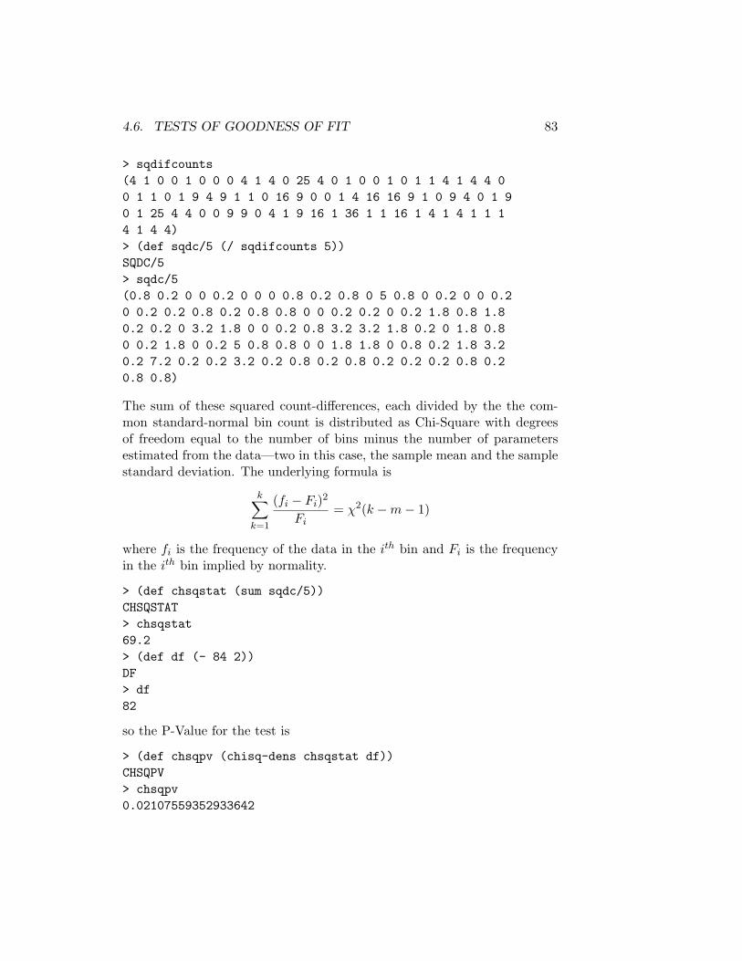
4.6. TESTS OF GOODNESS OF FIT 83
> sqdifcounts(4 1 0 0 1 0 0 0 4 1 4 0 25 4 0 1 0 0 1 0 1 1 4 1 4 4 00 1 1 0 1 9 4 9 1 1 0 16 9 0 0 1 4 16 16 9 1 0 9 4 0 1 90 1 25 4 4 0 0 9 9 0 4 1 9 16 1 36 1 1 16 1 4 1 4 1 1 14 1 4 4)> (def sqdc/5 (/ sqdifcounts 5))SQDC/5> sqdc/5(0.8 0.2 0 0 0.2 0 0 0 0.8 0.2 0.8 0 5 0.8 0 0.2 0 0 0.20 0.2 0.2 0.8 0.2 0.8 0.8 0 0 0.2 0.2 0 0.2 1.8 0.8 1.80.2 0.2 0 3.2 1.8 0 0 0.2 0.8 3.2 3.2 1.8 0.2 0 1.8 0.80 0.2 1.8 0 0.2 5 0.8 0.8 0 0 1.8 1.8 0 0.8 0.2 1.8 3.20.2 7.2 0.2 0.2 3.2 0.2 0.8 0.2 0.8 0.2 0.2 0.2 0.8 0.20.8 0.8)
The sum of these squared count-differences, each divided by the the com-mon standard-normal bin count is distributed as Chi-Square with degreesof freedom equal to the number of bins minus the number of parametersestimated from the data—two in this case, the sample mean and the samplestandard deviation. The underlying formula is
k∑
k=1
(fi − Fi)2
Fi= χ2(k −m− 1)
where fi is the frequency of the data in the ith bin and Fi is the frequencyin the ith bin implied by normality.
> (def chsqstat (sum sqdc/5))CHSQSTAT> chsqstat69.2> (def df (- 84 2))DF> df82
so the P-Value for the test is
> (def chsqpv (chisq-dens chsqstat df))CHSQPV> chsqpv0.02107559352933642
84 CHAPTER 4. HYPOTHESIS TESTS
We have to reject the null-hypothesis that the average test score data arenormally distributed at slightly above the 2% level. This calls into questionour hypothesis test concerning the magnitude of the standard deviation ofthese data. In real-world analysis we would have tested for normality beforedoing that particular hypothesis test.

Chapter 5
Linear Regression Analysis
This chapter focuses on the mechanics of OLS regression analysis. Readershaving difficulty with the material can obtain appropriate background byreading Chapters 4, 5, and 16 of the Stock and Watson textbook. Thosewho have difficulty with that material can first read Chapters 8, 9 and 10 ofmy Statistics for Economists: A Beginning. For background on matrix alge-bra, read Chapter 4 of Alpha Chiang’s mathematical economics textbook,1
or alternatively, Appendix A of the econometrics textbook by Johnston andDiNardo.2 We begin by working through the analysis using matrix calcu-lations. Then we show how to use the regression-model object provided byXLispStat. Issues regarding heteroskedasticity and serial correlation in theresiduals and the problem of multicollinearity are then discussed. And fi-nally, three new OLS regression functions useful for day-to-day econometricanalysis, together with some supporting functions, are presented.
1Alpha C. Chiang, Fundamental Methods of Mathematical Economics, Third Edition,McGraw-Hill, 1984, pages 54-88.
2Jack Johnston and John DiNardo, Econometric Methods, McGraw-Hill, 1997, pages455-67.
85
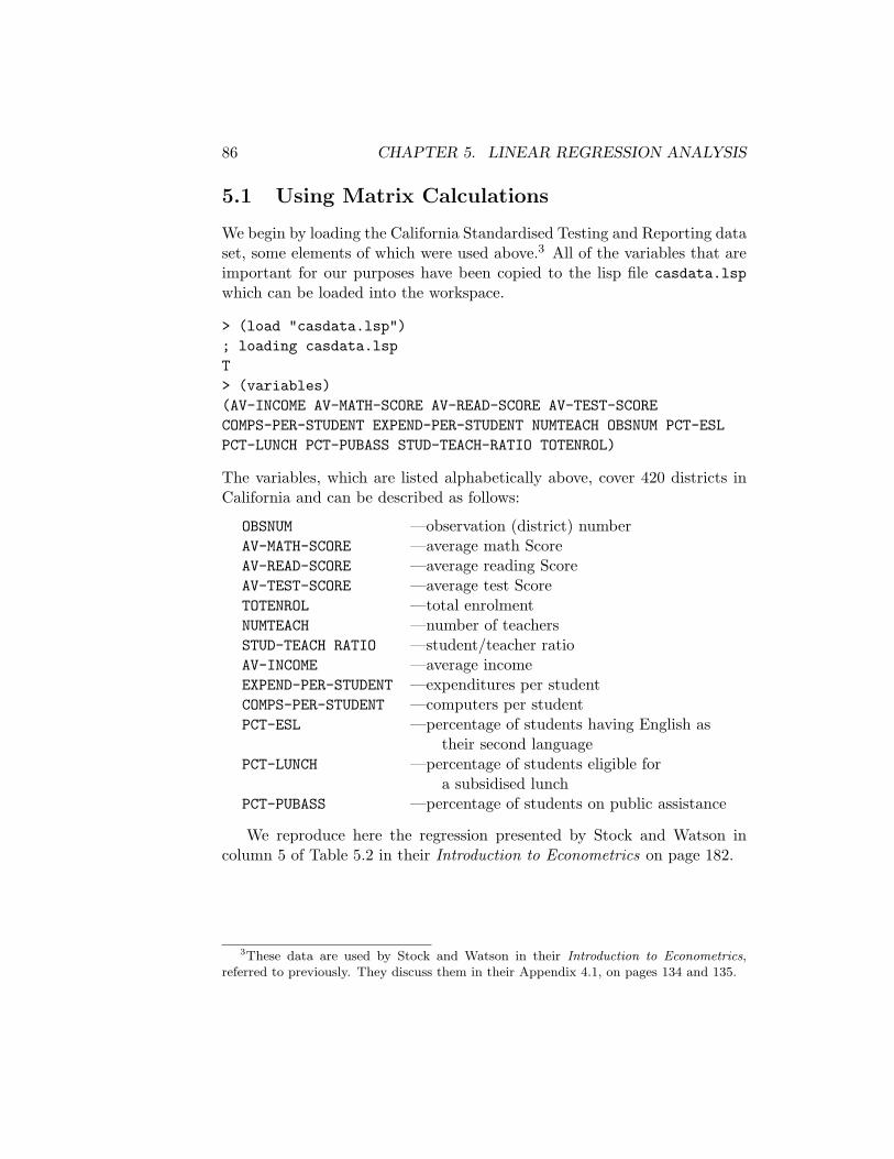
86 CHAPTER 5. LINEAR REGRESSION ANALYSIS
5.1 Using Matrix Calculations
We begin by loading the California Standardised Testing and Reporting dataset, some elements of which were used above.3 All of the variables that areimportant for our purposes have been copied to the lisp file casdata.lspwhich can be loaded into the workspace.
> (load "casdata.lsp"); loading casdata.lspT> (variables)(AV-INCOME AV-MATH-SCORE AV-READ-SCORE AV-TEST-SCORECOMPS-PER-STUDENT EXPEND-PER-STUDENT NUMTEACH OBSNUM PCT-ESLPCT-LUNCH PCT-PUBASS STUD-TEACH-RATIO TOTENROL)
The variables, which are listed alphabetically above, cover 420 districts inCalifornia and can be described as follows:
OBSNUM —observation (district) numberAV-MATH-SCORE —average math ScoreAV-READ-SCORE —average reading ScoreAV-TEST-SCORE —average test ScoreTOTENROL —total enrolmentNUMTEACH —number of teachersSTUD-TEACH RATIO —student/teacher ratioAV-INCOME —average incomeEXPEND-PER-STUDENT —expenditures per studentCOMPS-PER-STUDENT —computers per studentPCT-ESL —percentage of students having English as
their second languagePCT-LUNCH —percentage of students eligible for
a subsidised lunchPCT-PUBASS —percentage of students on public assistance
We reproduce here the regression presented by Stock and Watson incolumn 5 of Table 5.2 in their Introduction to Econometrics on page 182.
3These data are used by Stock and Watson in their Introduction to Econometrics,referred to previously. They discuss them in their Appendix 4.1, on pages 134 and 135.

5.1. USING MATRIX CALCULATIONS 87
To begin, we need an X matrix of independent variables, with the con-stant attached as the left-most column and a Y vector containing the de-pendent variable. We create Y using the coerce function, a vector of onesusing the repeat function and X using the bind-columns function.
> (def Y (coerce av-test-score ’vector))Y> (def const (repeat 1 (length Y)))CONST> (def X (bind-columns const stud-teach-ratio pct-esl pct-lunchpct-pubass))X
The formula for the vector of coefficients is
b = (X′X)−1X′Y
We program it using the transpose, matmult and inverse functions.
> (def xtr (transpose x))XTR> (def xtrx (matmult xtr x))XTRX> (def xtrxinv (inverse xtrx))XTRXINV> (def xtry (matmult xtr y))XTRY(def coeffs (matmult xtrxinv xtry))COEFFS> coeffs#(700.3942701828369 -1.0144897057204252 -0.1298071233417179-0.5286162083894679 -0.04786851798742055)
The residuals aree = Y −Xb
> (def resids (- y (matmult x coeffs)))RESIDS
and the sum of squared residuals is equal to e′e which is calculated usingthe inner-product function. The outer-product function would be usedto obtain ee′.
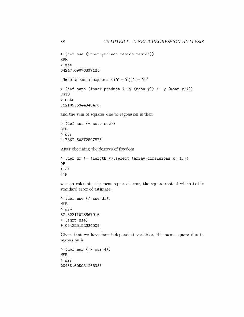
88 CHAPTER 5. LINEAR REGRESSION ANALYSIS
> (def sse (inner-product resids resids))SSE> sse34247.09076897185
The total sum of squares is (Y − Y)(Y − Y)′
> (def ssto (inner-product (- y (mean y)) (- y (mean y))))SSTO> ssto152109.5944940476
and the sum of squares due to regression is then
> (def ssr (- ssto sse))SSR> ssr117862.50372507575
After obtaining the degrees of freedom
> (def df (- (length y)(select (array-dimensions x) 1)))DF> df415
we can calculate the mean-squared error, the square-root of which is thestandard error of estimate.
> (def mse (/ sse df))MSE> mse82.52311028667916> (sqrt mse)9.084223152624508
Given that we have four independent variables, the mean square due toregression is
> (def msr ( / ssr 4))MSR> msr29465.625931268936

5.1. USING MATRIX CALCULATIONS 89
and the F-statistic for significance of the regression is
> (def fstat (/ msr mse))FSTAT> fstat357.0590811338489
The R2 is the ratio of the ‘explained variance’ to the total variance.
> (def rsq (/ ssr ssto))RSQ> rsq0.7748525273314563
To obtain the standard errors of the coefficient estimates we need the vari-ance covariance matrix of the coefficients which is
σ2(X′X)−1
> (def vcv (* mse xtrxinv))VCV
and which we can print out using the print-matrix function.
> (print-matrix vcv)#2a(
( 22.0701 -1.10682 2.051239E-2 -4.689474E-3 -1.879010E-2)( -1.10682 5.747246E-2 -8.080991E-4 -5.756423E-4 1.246380E-3)( 2.051239E-2 -8.080991E-4 1.155845E-3 -7.013666E-4 6.407913E-4)( -4.689474E-3 -5.756423E-4 -7.013666E-4 1.036224E-3 -1.454744E-3)( -1.879010E-2 1.246380E-3 6.407913E-4 -1.454744E-3 3.717387E-3)
)NIL
The slickest way to obtain the standard-errors of the coefficients is to createa list of zeros and then use the dotimes function to extract the diagonalelements of VCV and insert them in that vector using the select and setffunctions. This will produce a list giving the variances of the coefficients.
> (def varcoefs (repeat 0 (length coeffs)))VARCOEFS> varcoefs(0 0 0 0 0)

90 CHAPTER 5. LINEAR REGRESSION ANALYSIS
> (dotimes (i (length varcoefs))(setf (select varcoefs i)(aref vcv i i)))NIL> varcoefs(22.07009306717356 0.057472455848983015 0.00115584488736129560.0010362236138833243 0.00371738710011723)
The standard-errors of the coefficients can then be calculated by taking thesquare root of the list of variances.
> (def stdcoefs (sqrt varcoefs))STDCOEFS> stdcoefs(4.697881763856298 0.23973413576081112 0.0339977188552599150.032190427364098856 0.06097037887464068)
Finally, the t-ratios can be obtained by dividing coeffs by stdcoefs.
> (def trat (/ coeffs stdcoefs))TRAT> trat#(149.08724940065585 -4.231728212175038 -3.8181127355735796-16.42153434033062 -0.7851110468878918)
5.2 Using the Regression-Model Function
Of course there is an easier way to perform the above calculations—we cansimply use the regression-model function that comes with XLispStat.
> (regression-model (list stud-teach-ratio pct-esl pct-lunchpct-pubass) av-test-score)Least Squares Estimates:
Constant 700.394 (4.69788)Variable 0 -1.01449 (0.239734)Variable 1 -0.129807 (3.399772E-2)Variable 2 -0.528616 (3.219043E-2)Variable 3 -4.786852E-2 (6.097038E-2)
R Squared: 0.774853Sigma hat: 9.08422Number of cases: 420Degrees of freedom: 415
#<Object: 82c9520, prototype = REGRESSION-MODEL-PROTO>
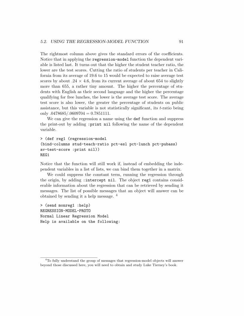
5.2. USING THE REGRESSION-MODEL FUNCTION 91
The rightmost column above gives the standard errors of the coefficients.Notice that in applying the regression-model function the dependent vari-able is listed last. It turns out that the higher the student teacher ratio, thelower are the test scores. Cutting the ratio of students per teacher in Cali-fornia from its average of 19.6 to 15 would be expected to raise average testscores by about .24 × 4.6, from its current average of about 654 to slightlymore than 655, a rather tiny amount. The higher the percentage of stu-dents with English as their second language and the higher the percentagequalifying for free lunches, the lower is the average test score. The averagetest score is also lower, the greater the percentage of students on publicassistance, but this variable is not statistically significant, its t-ratio beingonly .0478685/.0609704 = 0.7851111.
We can give the regression a name using the def function and suppressthe print-out by adding :print nil following the name of the dependentvariable.
> (def reg1 (regression-model(bind-columns stud-teach-ratio pct-esl pct-lunch pct-pubass)av-test-score :print nil))REG1
Notice that the function will still work if, instead of embedding the inde-pendent variables in a list of lists, we can bind them together in a matrix.
We could suppress the constant term, running the regression throughthe origin, by adding :intercept nil. The object reg1 contains consid-erable information about the regression that can be retrieved by sending itmessages. The list of possible messages that an object will answer can beobtained by sending it a help message. 4
> (send monreg1 :help)REGRESSION-MODEL-PROTONormal Linear Regression ModelHelp is available on the following:
4To fully understand the group of messages that regression-model objects will answerbeyond those discussed here, you will need to obtain and study Luke Tierney’s book.
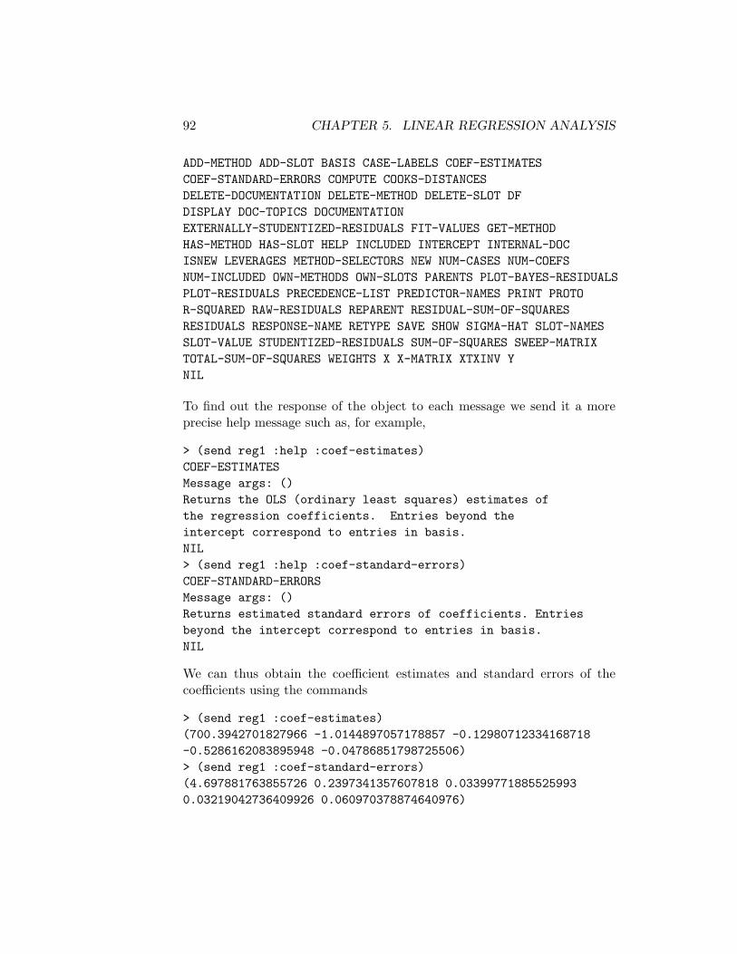
92 CHAPTER 5. LINEAR REGRESSION ANALYSIS
ADD-METHOD ADD-SLOT BASIS CASE-LABELS COEF-ESTIMATESCOEF-STANDARD-ERRORS COMPUTE COOKS-DISTANCESDELETE-DOCUMENTATION DELETE-METHOD DELETE-SLOT DFDISPLAY DOC-TOPICS DOCUMENTATIONEXTERNALLY-STUDENTIZED-RESIDUALS FIT-VALUES GET-METHODHAS-METHOD HAS-SLOT HELP INCLUDED INTERCEPT INTERNAL-DOCISNEW LEVERAGES METHOD-SELECTORS NEW NUM-CASES NUM-COEFSNUM-INCLUDED OWN-METHODS OWN-SLOTS PARENTS PLOT-BAYES-RESIDUALSPLOT-RESIDUALS PRECEDENCE-LIST PREDICTOR-NAMES PRINT PROTOR-SQUARED RAW-RESIDUALS REPARENT RESIDUAL-SUM-OF-SQUARESRESIDUALS RESPONSE-NAME RETYPE SAVE SHOW SIGMA-HAT SLOT-NAMESSLOT-VALUE STUDENTIZED-RESIDUALS SUM-OF-SQUARES SWEEP-MATRIXTOTAL-SUM-OF-SQUARES WEIGHTS X X-MATRIX XTXINV YNIL
To find out the response of the object to each message we send it a moreprecise help message such as, for example,
> (send reg1 :help :coef-estimates)COEF-ESTIMATESMessage args: ()Returns the OLS (ordinary least squares) estimates ofthe regression coefficients. Entries beyond theintercept correspond to entries in basis.NIL> (send reg1 :help :coef-standard-errors)COEF-STANDARD-ERRORSMessage args: ()Returns estimated standard errors of coefficients. Entriesbeyond the intercept correspond to entries in basis.NIL
We can thus obtain the coefficient estimates and standard errors of thecoefficients using the commands
> (send reg1 :coef-estimates)(700.3942701827966 -1.0144897057178857 -0.12980712334168718-0.5286162083895948 -0.04786851798725506)> (send reg1 :coef-standard-errors)(4.697881763855726 0.2397341357607818 0.033997718855259930.03219042736409926 0.060970378874640976)

5.3. HETEROSKEDASTICITY 93
And we can calculate the t-ratios by manipulating the Interpreter’s answersto expressions sent to the regression-model object.
> (def t-ratios (/ (send reg1 :coef-estimates)(send reg1 :coef-standard-errors)))T-RATIOS> t-ratios(149.08724940066543 -4.231728212164962 -3.8181127355726745-16.421534340334357 -0.7851110468851737)
If the degrees of freedom are sufficient, say 30 or more, a t-ratio in excessof 2 will indicate the presence of a statistically significant relationship. Ofcourse the exact P-Value can be found using the t-cdf function.
5.3 Heteroskedasticity
Standard regression analysis assumes that the regression residuals have aconstant variance—that is, are homoskedastic. This assumption is oftenviolated with the regression residuals being, in fact, heteroskedastic. Theresiduals from the regression above are plotted as follows.
> (send reg1 :plot-residuals)#<Object: 82e66a0, prototype = SCATTERPLOT-PROTO>
and shown in Figure 11. The fitted values of the dependent variable arealong the horizontal axis.
A formal test for heteroskedasticity is the Breusch-Pagan test, whichinvolves OLS estimation of
e2i = α + β1X1i + β2X2i + ... + ui
where the ei are the regression residuals, the X1i, X2i ... etc. are some orall of the independent variables in the original regression, and the ui are theresiduals of the Breusch-Pagan regression.5 The test can be implementedusing the following code.
> (def resids (send reg1 :residuals))RESIDS> (def residssq (^ resids 2))RESIDSSQ
5T. S. Breusch and A. R. Pagan, “A Simple Test for Heteroskedasticity and RandomCoefficient Variation,” Econometrica, Vol. 47, 1979, pages 1287-1294.

94 CHAPTER 5. LINEAR REGRESSION ANALYSIS
Figure 11: Regression residuals plotted against fitted values
> (def reg2 (regression-model(list stud-teach-ratio pct-esl pct-lunch pct-pubass)residssq))
Least Squares Estimates:
Constant 251.339 (69.3074)Variable 0 -7.55048 (3.53677)Variable 1 -0.194234 (0.501565)Variable 2 -0.139801 (0.474902)Variable 3 -0.920295 (0.899490)
R Squared: 2.638079E-2Sigma hat: 134.019Number of cases: 420Degrees of freedom: 415
REG2> (def RSQ (send reg2 :R-squared))RSQ

5.4. TIME SERIES: AUTOCORRELATED RESIDUALS 95
> (def chisqstat (* (length resids) RSQ))CHISQSTAT> chisqstat11.079932837242543> (def Pval (- 1 (chisq-cdf chisqstat 4)))PVAL> pval0.025680216026914393
The null-hypothesis of homoskedasticity can be rejected at the 5% level. Ihave written a Breusch-Pagan function to calculate the Breusch-Paganstatistic. The function’s first argument is the name of the regression-modelthat generated the residuals being tested. Its second argument is a namedmatrix containing some or all of the independent variables, and its thirdargument is set to 1 to print the results or to 0 to forego printing. Thefunction is applied as follows.
> (def indepvars (bind-columns stud-teach-ratio pct-esl pct-lunchpct-pubass)INDEPVARS> (Breusch-Pagan reg1 indepvars 1)
Breusch-Pagan test on the ResidualsChi-Square Statistic = 11.079932837242543P-Value = 0.025680216026914393
If one wants to use all the independent variables in the Breusch-Pagan test,the indepvars variable can constructed and used in the original regression.Of course, a constant is automatically added to all regressions we run unlesswe specify otherwise.
5.4 Time Series: Autocorrelated Residuals
Regressions involving time series often suffer from serial correlation in theresiduals. This violates the standard OLS requirement that the regres-sion residuals be independently distributed. To deal with these issues weutilise a data set containing numerous Canadian macroeconomic variablesto estimate that country’s demand function for money. More series thanwe actually use are included in the dataset, which is contained in the filecamoinpr.lsp, so that the reader can experiment using alternative regres-sions and other statistical calculations.
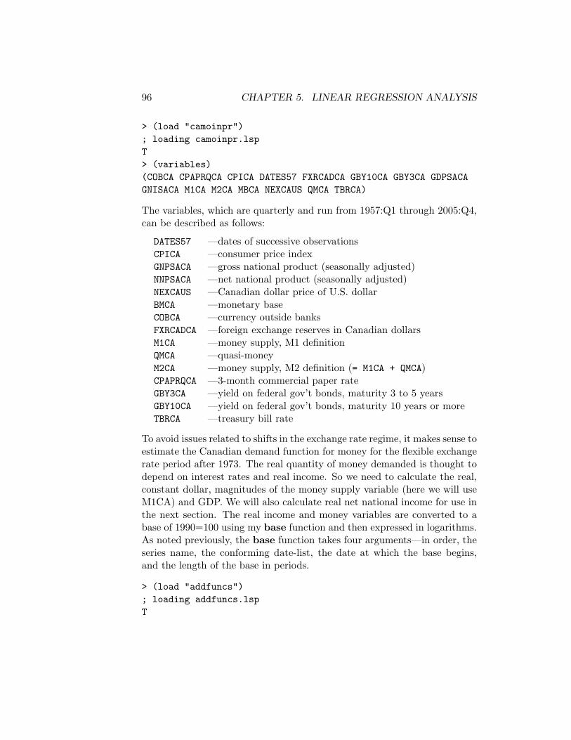
96 CHAPTER 5. LINEAR REGRESSION ANALYSIS
> (load "camoinpr"); loading camoinpr.lspT> (variables)(COBCA CPAPRQCA CPICA DATES57 FXRCADCA GBY10CA GBY3CA GDPSACAGNISACA M1CA M2CA MBCA NEXCAUS QMCA TBRCA)
The variables, which are quarterly and run from 1957:Q1 through 2005:Q4,can be described as follows:
DATES57 —dates of successive observationsCPICA —consumer price indexGNPSACA —gross national product (seasonally adjusted)NNPSACA —net national product (seasonally adjusted)NEXCAUS —Canadian dollar price of U.S. dollarBMCA —monetary baseCOBCA —currency outside banksFXRCADCA —foreign exchange reserves in Canadian dollarsM1CA —money supply, M1 definitionQMCA —quasi-moneyM2CA —money supply, M2 definition (= M1CA + QMCA)CPAPRQCA —3-month commercial paper rateGBY3CA —yield on federal gov’t bonds, maturity 3 to 5 yearsGBY10CA —yield on federal gov’t bonds, maturity 10 years or moreTBRCA —treasury bill rate
To avoid issues related to shifts in the exchange rate regime, it makes sense toestimate the Canadian demand function for money for the flexible exchangerate period after 1973. The real quantity of money demanded is thought todepend on interest rates and real income. So we need to calculate the real,constant dollar, magnitudes of the money supply variable (here we will useM1CA) and GDP. We will also calculate real net national income for use inthe next section. The real income and money variables are converted to abase of 1990=100 using my base function and then expressed in logarithms.As noted previously, the base function takes four arguments—in order, theseries name, the conforming date-list, the date at which the base begins,and the length of the base in periods.
> (load "addfuncs"); loading addfuncs.lspT

5.4. TIME SERIES: AUTOCORRELATED RESIDUALS 97
> (def rm1ca (/ m1ca cpica))RM1CA> (def rgdpca (/ gdpsaca cpica))RGDPCA> (def rgnica (/ gnisaca cpica))RGNICA> (def rm1ca (log (base rm1ca dates57 1990.0 4)))RM1CA> (def rgdpca (log (base rgdpca dates57 1990.0 4)))RGDPCA> (def rgnica (log (base rgnica dates57 1990.0 4)))RGNICA
Since we are going to run regressions on the data following 1973, we needto remove the prior years from the data series and date list.
> (def obs2del (date2obs dates57 1974))OBS2DEL> (def newdate (remove-first obs2del dates57))NEWDATE> (first-five newdate)(1974.0 1974.25 1974.5 1974.75 1975.0)> (last-five newdate)(2004.75 2005.0 2005.25 2005.5 2005.75)> (def rm1ca (remove-first obs2del rm1ca))RM1CA> (def rgdpca (remove-first obs2del rgdpca))RGDPCA> (def rgnica (remove-first obs2del rgnica))RGNICA> (def cpaprqca (remove-first obs2del cpaprqca))CPAPRQCA
As indicated by the last command above, the interest rate being used is the3-month commercial paper rate.
Since the M1 variable is not seasonally adjusted, we should incorpo-rate seasonal dummy-variables (each taking a value of 1 for a particularquarter and zero for all other quarters) in the analysis. My two functionsseasdums-Q and seasdums-M both take two arguments—in order, thedate list to which the seasonal dummy-variables must conform, and the
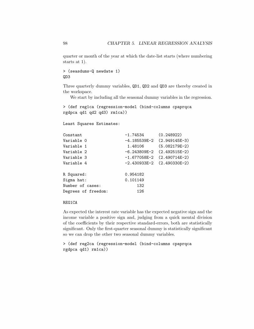
98 CHAPTER 5. LINEAR REGRESSION ANALYSIS
quarter or month of the year at which the date-list starts (where numberingstarts at 1).
> (seasdums-Q newdate 1)QD3
Three quarterly dummy variables, QD1, QD2 and QD3 are thereby created inthe workspace.
We start by including all the seasonal dummy variables in the regression.
> (def reg1ca (regression-model (bind-columns cpaprqcargdpca qd1 qd2 qd3) rm1ca))
Least Squares Estimates:
Constant -1.74534 (0.248922)Variable 0 -4.185539E-2 (2.949145E-3)Variable 1 1.48106 (5.082179E-2)Variable 2 -6.243809E-2 (2.492515E-2)Variable 3 -1.677058E-2 (2.490714E-2)Variable 4 -2.430933E-2 (2.490330E-2)
R Squared: 0.954182Sigma hat: 0.101149Number of cases: 132Degrees of freedom: 126
REG1CA
As expected the interest rate variable has the expected negative sign and theincome variable a positive sign and, judging from a quick mental divisionof the coefficients by their respective standard-errors, both are statisticallysignificant. Only the first-quarter seasonal dummy is statistically significantso we can drop the other two seasonal dummy variables.
> (def reg2ca (regression-model (bind-columns cpaprqcargdpca qd1) rm1ca))

5.4. TIME SERIES: AUTOCORRELATED RESIDUALS 99
Least Squares Estimates:
Constant -1.76207 (0.247243)Variable 0 -4.185308E-2 (2.937437E-3)Variable 1 1.48172 (5.061157E-2)Variable 2 -4.873644E-2 (2.027082E-2)
R Squared: 0.953819Sigma hat: 0.100753Number of cases: 132Degrees of freedom: 128
REG2CA> (plot-lines (- newdate 1900)(send reg2ca :residuals))#<Object: 81447f8, prototype = SCATTERPLOT-PROTO>> ; saving postscript image to file resca1.ps...done
As can be seen from the plot of the residuals in Figure 12, serial correlationis clearly present—if the residual in a particular period takes a high value,the residual in the next period also tends to take a high value.
Figure 12: Residuals from regression reg2ca residualsplotted against time

100 CHAPTER 5. LINEAR REGRESSION ANALYSIS
We need a test for the presence of serial correlation in the residualsof a regression. Historically, the standard approach has been to calculatethe Durbin-Watson statistic, but this test is imprecise. Instead, we usea Lagrange-Multiplier-based test which involves regressing the residuals ofthe regression on themselves lagged and the X matrix and then testing thenull-hypothesis that the coefficient of the lagged residuals is zero.6
et = Xβ + ρ et−1 + ut
where the matrix X is the matrix of independent variables, including theconstant term, and et is the vector of residuals, from the original regression.The null-hypothesis is that ρ equals zero. Additional lags of the residualscan be added to test for higher order serial correlation. In that case, thenull-hypothesis is that the coefficients of all the lagged residuals are zero.To perform this test, we use my LMSC-test function which takes three argu-ments, the name of the regression whose residuals are being tested followedby the number of lagged error terms (i.e., the order of the test), followed bya 1 if we want the output to be printed and zero otherwise.7 A first-ordertest of the residuals of regression reg3ca yields the following.
> (LMSC-test reg2ca 1 1)LM-Based Test for Serial Correlation in Residuals:Order = 1 Chisq-stat = 507.5464949337206 P-Value = 0.0NIL
The Chi-square test statistic here is based upon the calculation of an F-statistic in a manner that will be discussed at the end of the next sectiondealing with multicollinearity.
To test for higher-order serial correlation in the residuals, we simply addlags to the above test.
> (LMSC-test reg2ca 2 1)LM-Based Test for Serial Correlation in Residuals:Order =< 2 Chisq-stat = 480.44135388615615 P-Value = 0.0
6The origins of this test go back to work by Breusch and Godfrey in the 1970s. SeeT. S. Breusch, “Testing for Autocorrelation in Dynamic Linear Models,” Australian Eco-nomic Papers, Vol. 17, 1978, pp. 334-355, and L. G. Godfrey, “Testing for Higher Order Se-rial Correlation in Regression Equations When the Regressors Include Lagged DependentVariables,” Econometrica, Vol. 46, pp. 1303-1310. The nature of the Lagrange-Multiplierprinciple is beyond the depth of discussion here.
7The only time we would not want the output printed would be when we are embeddingthe function inside another function that uses its output.

5.4. TIME SERIES: AUTOCORRELATED RESIDUALS 101
> (LMSC-test reg2ca 5 1)LM-Based Test for Serial Correlation in Residuals:Order =< 5 Chisq-stat = 373.66268475177554 P-Value = 0.0
> (LMSC-test reg2ca 10 1)LM-Based Test for Serial Correlation in Residuals:Order =< 10 Chisq-stat = 238.34777770689487 P-Value = 0.0
> (LMSC-test reg2ca 15 1)LM-Based Test for Serial Correlation in Residuals:Order =< 15 Chisq-stat = 156.01194523891323 P-Value = 0.0
> (LMSC-test reg2ca 20 1)LM-Based Test for Serial Correlation in Residuals:Order =< 20 Chisq-stat = 140.13010399933057 P-Value = 0.0
Actually, one need only apply the function until a lag is reached at which theabsence of serial correlation can be rejected since once the null hypothesiscan be rejected at a given lag, it will necessarily be rejected at higher lags.The hypothesis of no serial correlation in the above residuals can be easilyrejected—the above P-Values are so small that the XLispStat Interpretercannot distinguish them from zero.
The observed serial correlation may result either from the omission ofserially correlated variables affecting the demand for money or from a mis-specification of the form of the regression function. It is generally believedthat serial correlation of the residuals from demand function for money es-timation arises because the process of adjustment of the real money supplyto a shift in the quantity of nominal money involves changes in the pricelevel that occur only slowly—until the price level has adjusted the residualsof the regression will remain close to each other and only gradually declinetoward their mean of zero.
To perform a test for autocorrelation in time series other than the resid-uals from a regression, we can use the Ljung-Box Q test. The formula is
Q = T (T + 2)k=s∑
k=1
r2k/(T − k)
where r2k is the kth autocorrelation, T is the sample size, and s is the lag
length, equal to no more than T/4 rounded down to the next integer.8 Fordoing this test, I wrote a function LBQ that takes three arguments—inorder, the name of the time series being tested, the number of lags, and a
8For a discussion of this formula, see pages 86-87 of the textbook by Walter Endersreferred to earlier.

102 CHAPTER 5. LINEAR REGRESSION ANALYSIS
degrees-of-freedom adjustment which for present purposes should be fixedat zero.9
5.5 Multicollinearity
Suppose that a researcher is estimating the demand function for money forCanada using annual data from 1974 to 1996 and does a dumb thing—usesboth real GDP and real GNI as dependent variables! To demonstrate whatwill happen, we need to convert the relevant quarterly series to an annualaverage bases using my q2a-avg function and reduce their length so thatthey start in 1974 and stop at 1996.
> (def rm1ca (remove-last 8 (q2a-avg (remove-first 4 rm1ca)0 1974 2004)))RM1CA> (def rgdpca (remove-last 8 (q2a-avg (remove-first 4 rgdpca)0 1974 2004)))RGDPCA> (def rgnica (remove-last 8 (q2a-avg (remove-first 4 rgnica)0 1974 2004)))RGNICA> (def cpaprqca (remove-last 8 (q2a-avg (remove-first 4cpaprqca) 0 1974 2004)))CPAPRQCA> (def anndates (setdates rm1ca 1974 1))ANNDATES
As noted earlier, the q2a-avg and m2q-avg functions take four arguments—in order, the series list being transformed, the observation of the originalseries at which to start the transformation, the first date of the resultingtransformed series and the last date of the transformed series.
The regression the researcher runs is then
9This degrees of freedom adjustment parameter is set above zero when the residualsfrom an auto-regressive-moving-average process are being tested.
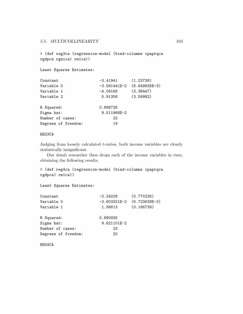
5.5. MULTICOLLINEARITY 103
> (def reg3ca (regression-model (bind-columns cpaprqcargdpca rgnica) rm1ca))
Least Squares Estimates:
Constant -3.41941 (1.23738)Variable 0 -3.581441E-2 (6.649835E-3)Variable 1 -4.09166 (3.38447)Variable 2 5.91358 (3.59982)
R Squared: 0.898726Sigma hat: 9.511968E-2Number of cases: 23Degrees of freedom: 19
REG3CA
Judging from loosely calculated t-ratios, both income variables are clearlystatistically insignificant.
Our dumb researcher then drops each of the income variables in turn,obtaining the following results.
> (def reg4ca (regression-model (bind-columns cpaprqcargdpca) rm1ca))
Least Squares Estimates:
Constant -2.24029 (0.770226)Variable 0 -3.603321E-2 (6.723639E-3)Variable 1 1.56613 (0.166739)
R Squared: 0.890935Sigma hat: 9.621101E-2Number of cases: 23Degrees of freedom: 20
REG4CA
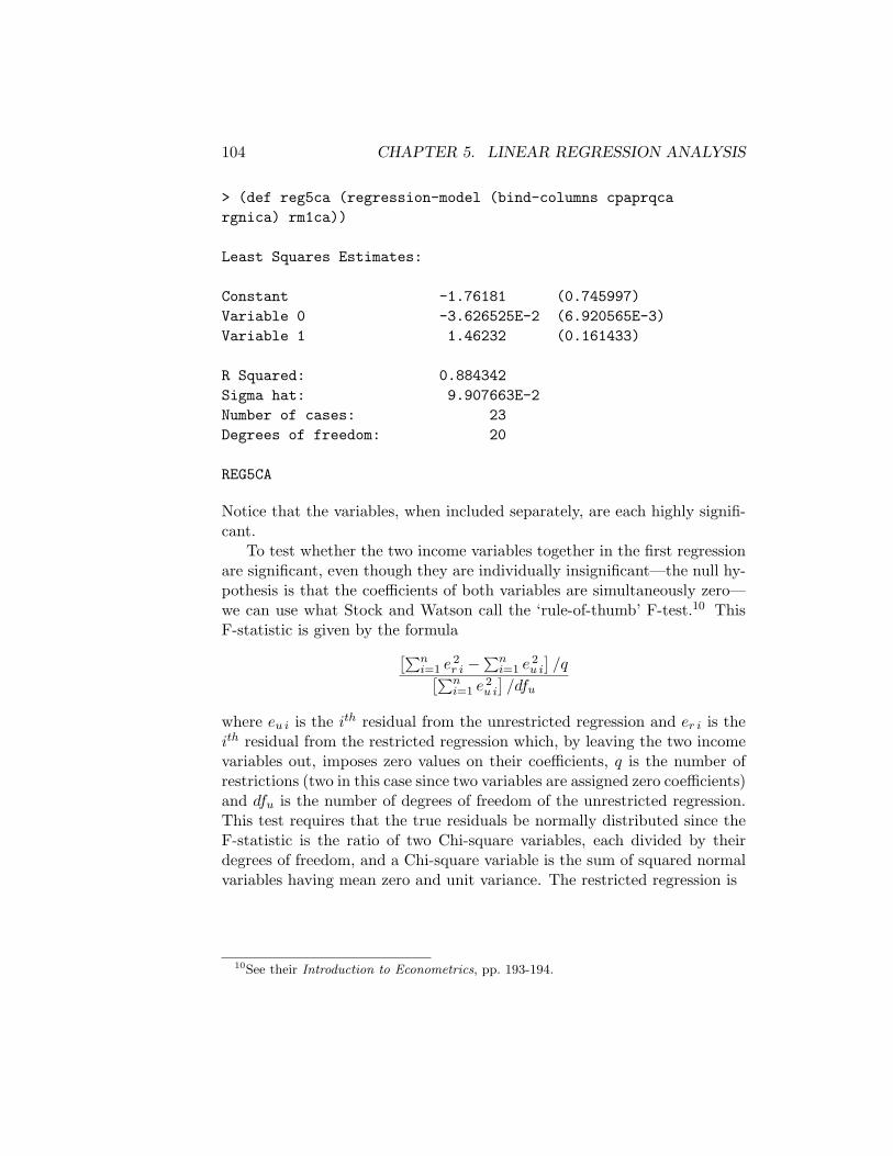
104 CHAPTER 5. LINEAR REGRESSION ANALYSIS
> (def reg5ca (regression-model (bind-columns cpaprqcargnica) rm1ca))
Least Squares Estimates:
Constant -1.76181 (0.745997)Variable 0 -3.626525E-2 (6.920565E-3)Variable 1 1.46232 (0.161433)
R Squared: 0.884342Sigma hat: 9.907663E-2Number of cases: 23Degrees of freedom: 20
REG5CA
Notice that the variables, when included separately, are each highly signifi-cant.
To test whether the two income variables together in the first regressionare significant, even though they are individually insignificant—the null hy-pothesis is that the coefficients of both variables are simultaneously zero—we can use what Stock and Watson call the ‘rule-of-thumb’ F-test.10 ThisF-statistic is given by the formula
[∑ni=1 e 2
r i −∑n
i=1 e 2u i
]/q[∑n
i=1 e 2u i
]/dfu
where eu i is the ith residual from the unrestricted regression and er i is theith residual from the restricted regression which, by leaving the two incomevariables out, imposes zero values on their coefficients, q is the number ofrestrictions (two in this case since two variables are assigned zero coefficients)and dfu is the number of degrees of freedom of the unrestricted regression.This test requires that the true residuals be normally distributed since theF-statistic is the ratio of two Chi-square variables, each divided by theirdegrees of freedom, and a Chi-square variable is the sum of squared normalvariables having mean zero and unit variance. The restricted regression is
10See their Introduction to Econometrics, pp. 193-194.
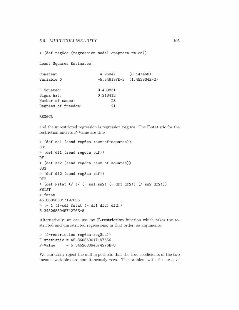
5.5. MULTICOLLINEARITY 105
> (def reg6ca (regression-model cpaprqca rm1ca))
Least Squares Estimates:
Constant 4.96847 (0.147468)Variable 0 -5.546137E-2 (1.452334E-2)
R Squared: 0.409831Sigma hat: 0.218412Number of cases: 23Degrees of freedom: 21
REG6CA
and the unrestricted regression is regression reg3ca. The F-statistic for therestriction and its P-Value are thus
> (def ss1 (send reg6ca :sum-of-squares))SS1> (def df1 (send reg6ca :df))DF1> (def ss2 (send reg3ca :sum-of-squares))SS2> (def df2 (send reg3ca :df))DF2> (def Fstat (/ (/ (- ss1 ss2) (- df1 df2)) (/ ss2 df2)))FSTAT> fstat45.860563017197656> (- 1 (f-cdf fstat (- df1 df2) df2))5.345268394574276E-8
Alternatively, we can use my F-restriction function which takes the re-stricted and unrestricted regressions, in that order, as arguments.
> (f-restriction reg6ca reg3ca))F-statistic = 45.860563017197656P-Value = 5.345268394574276E-8
We can easily reject the null-hypothesis that the true coefficients of the twoincome variables are simultaneously zero. The problem with this test, of

106 CHAPTER 5. LINEAR REGRESSION ANALYSIS
course, is that it assumes that the true residuals are independently nor-mally distributed, and we have every reason to believe that they are not.Nevertheless, we have learned how to run a ‘rule of thumb’ F-test. And wecan more easily determine if multicollinearity exists without running thistest. If each variable is significant when included by itself in the regression,the two together must be jointly significant when both are included—theproblem is that each variable is, in effect, waiting for the other one to relateto the dependent variable with the result that neither are significant.
Multicollinearity arises because two variables are so highly correlatedwith each other that the difference between them has no effect on the de-pendent variable, making it impossible, when both are included, for themto separately explain it—each is insignificant once the other is included.To visualise this, run my multicollinearity function, which takes no ar-guments. Two graphs will appear, one on top of the other. Imagine Y asthe dependent variable, and click repeatedly on the yaw buttons of the twographs. You will observe a clear regression plane in the X,Z dimension on theno multicollinearity graph while no such plane can be clearly defined onthe multicollinearity graph.
Our Lagrange Multiplier-based test for serial correlation discussed in theprevious section also uses the above ‘rule of thumb’ F-statistic to test thesignificance of the group of coefficients of the lagged values of the error term.That test is a ‘large sample’ test—that is, it’s accuracy is only precise whenthe sample size is very large. To compensate for situations in which thesample is not large, the test calculates the P-Value under the assumptionthat the degrees of freedom in the denominator of the F-statistic are infinite.This will tend to make the P-Value smaller than it would be if we were touse the degrees of freedom of the unrestricted regression in the denominator,making us compensate for the small sample size by rejecting more often thenull-hypothesis of no serial correlation. It turns out that when the degreesof freedom in the denominator of the F-statistic are infinite, the F-statisticmultiplied by the number of restrictions (which will equal the degrees offreedom in its numerator) is distributed as Chi-Square with degrees of free-dom equal to that number of restrictions. We therefore used the Chi-Squaredistribution to calculate the P-Value in the LMSC-test function, settingthe test statistic equal to the number of restrictions times the F-statistic.

5.6. SOME IMPROVED LINEAR REGRESSION FUNCTIONS 107
5.6 Some Improved Linear Regression Functions
Our first task here is to be able to adjust the standard-errors of the re-gression coefficients to compensate, where necessary, for the presence ofheteroskedasticity and autocorrelation in the residuals. When the residualsare homoskedastic, the variance-covariance matrix of the coefficients is
V = s 2(X′X)−1
where s 2 =∑T
t=1 u 2t /(T − k − 1) is our point estimate of the variance of
the error-term ut, T is the number of observations, and k is the number ofparameters estimated, given by the number of columns in the matrix X.
When the residuals are heteroskedastic, but serially uncorrelated, we cal-culate this variance-covariance matrix using a formula developed by White11
V =
[T∑
t=1
xtx′t
]−1 [T∑
t=1
u2txtx′t
] [T∑
t=1
xtx′t
]−1
where the xt are the rows of X and, therefore,
[T∑
t=1
xtx′t
]−1
= (X′X)−1
When the error terms are homoskedastic, the ut and xt are uncorrelated andthis expression for V reduces to the previous one for V when the sample sizeis large. When there is serial correlation in the residuals, we follow Neweyand West, calculating the variance-covariance matrix of the coefficients as12
V =
[T∑
t=1
xtx′t
]−1 [T∑
t=1
u2txtx′t
+q∑
v=1
[1− v
q + 1
] T∑
t=v+1
(xtutut−vx′t + xt−vut−vutx′t)
[T∑
t=1
xtx′t
]−1
where q is the number of lags beyond which no serial correlation is present.Following Stock and Watson, we routinely set q equal to .75 T 1/3, rounded
11Halbert White, ”A Heteroskedasticity-Consistent Covariance Matrix Estimator and aDirect Test for Heteroskedasticity,” Econometrica, Vol. 48, 1980, pp. 827-838. See pages124-129 and 613-614 of the Stock and Watson book, Introduction to Econometrics, for adiscussion and the formula.
12Whitney Newey and Kenneth West, “A Simple Positive Semi-Definite, Heteroskedasticand Autocorrelation Consistent Covariance Matrix,” Econometrica, Vol. 55, 1987, pp. 703-708. See pages 502-507 of the book by Stock and Watson for a discussion, and equation10.5.21 on page 283 in Hamilton’s Time Series Analysis for the formula.

108 CHAPTER 5. LINEAR REGRESSION ANALYSIS
down to the nearest integer. If serial correlation is not present in the resid-uals, and we therefore set q = 0, the term [1 - v/(q + 1)] goes to zero andthe expression reverts to the previous one.
To perform the above calculations I have written a HAC-stderrs func-tion which takes two arguments—first the name of the regression object andsecond the number of lags. Setting the number of lags equal to zero resultsin an heteroskedasticity-only test. The function leaves a number of generi-cally named variables in the workspace, overwriting any previous variableshaving these names. Of particular interest are the variables stderrs andtratios.
5.6.1 A Basic OLS-Regression Function
To facilitate the incorporation of heteroskedasticity-and-autocorrelation-con-sistent standard errors in our regression analysis and to produce a muchbetter print-out of regression results, I have written some new functions.The first is the OLS-basic function which calculates and prints out a re-gression for which the user can decide whether to adjust the coefficientstandard-errors for heteroskedasticity and autocorrelation. It takes four ar-guments. The first is the name of the dependent variable and the second isa matrix of independent variables excluding the constant term. The thirdargument must be set to 0 to suppress the inclusion of a constant term andto 1 otherwise. The fourth argument is to be set equal to -1 if the resid-uals are to be treated as homoskedastic, to 0 if the errors are assumed tobe heteroskedastic, and to the magnitude of the highest lag for which theresiduals are assumed to be autocorrelated if the coefficient standard-errorsare to be made autocorrelation-consistent. In this case, I normally set thetruncation lag equal to the magnitude suggested above by Stock and Wat-son. This function also requires that the workspace contain a string objectcalled regressand consisting of the name of the dependent variable and alist of strings called regressors containing the names of the independentvariables.
To test this function, we first run the previously presented Stock-Watsonregression to test for heteroskedasticity.
> (load "addfuncs"); loading addfuncs.lspT> (load "casdata"); loading casdata.lsp

5.6. SOME IMPROVED LINEAR REGRESSION FUNCTIONS 109
T> (def regressand "Average Test Score")REGRESSAND> (def regressors (list "Constant" "Studs/Teach" "Pct. ESL""Pct. Free Lunch" "Pct. PubAss"))REGRESSORS> (OLS-basic av-test-score (bind-columns stud-teach-ratio pct-esl pct-lunchpct-pubass) 1 -1)
LINEAR REGRESSION
Dependent Variable: Average Test Score
Coefficient Std. Error T-stat P-Val
Constant 700.394 4.698 149.087 0.000Studs/Teach -1.014 0.240 -4.232 0.000Pct. ESL -0.130 0.034 -3.818 0.000Pct. Free Lunch -0.529 0.032 -16.422 0.000Pct. PubAss -0.048 0.061 -0.785 0.433
Number of Observations: 420Degrees of Freedom: 415R-Squared: 0.7748525273314566Adjusted R-Squared: 0.7726824312093502Sum of Squared Errors: 34247.090768971764LMSC -- Chi-Square: 42.26483384247289P-Value: 7.971312498966654E-11
Breusch-Pagan -- Chi-Square: 11.079932837242543P-Value: 0.025680216026914393
Regression F-Statistic: 357.0590811338497P-Value: 0.0
NIL
> (OLS-basic av-test-score (bind-columns stud-teach-ratio pct-esl pct-lunchpct-pubass) 1 0)
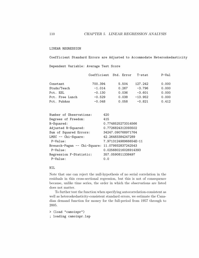
110 CHAPTER 5. LINEAR REGRESSION ANALYSIS
LINEAR REGRESSION
Coefficient Standard Errors are Adjusted to Accommodate Heteroskedasticity
Dependent Variable: Average Test Score
Coefficient Std. Error T-stat P-Val
Constant 700.394 5.504 127.242 0.000Studs/Teach -1.014 0.267 -3.796 0.000Pct. ESL -0.130 0.036 -3.601 0.000Pct. Free Lunch -0.529 0.038 -13.952 0.000Pct. PubAss -0.048 0.058 -0.821 0.412
Number of Observations: 420Degrees of Freedom: 415R-Squared: 0.7748525273314566Adjusted R-Squared: 0.7726824312093502Sum of Squared Errors: 34247.090768971764LMSC -- Chi-Square: 42.26483384247289P-Value: 7.971312498966654E-11Breusch-Pagan -- Chi-Square: 11.079932837242543P-Value: 0.025680216026914393Regression F-Statistic: 357.0590811338497P-Value: 0.0
NIL
Note that one can reject the null-hypothesis of no serial correlation in theresiduals in this cross-sectional regression, but this is not of consequencebecause, unlike time series, the order in which the observations are listeddoes not matter.
To further test the function when specifying autocorrelation-consistent aswell as heteroskedasticity-consistent standard errors, we estimate the Cana-dian demand function for money for the full-period from 1957 through to2005.
> (load "camoinpr"); loading camoinpr.lsp

5.6. SOME IMPROVED LINEAR REGRESSION FUNCTIONS 111
T> (seasdums-Q dates57 1)QD3> (def rm1ca (/ m1ca cpica))RM1CA> (def rgdpca (/ gdpsaca cpica))RGDPCA> (def regressand "Real M1")REGRESSAND> (def regressors (list "Constant" "Interest Rate" "Real GDP" "QD1"))REGRESSORS> (OLS-basic (log rm1ca)(bind-columns cpaprqca (log rgdpca) qd1) 1 -1)
LINEAR REGRESSION
Dependent Variable: Real M1
Coefficient Std. Error T-stat P-Val
Constant -1.762 0.037 -47.179 0.000Interest Rate -0.053 0.003 -19.930 0.000Real GDP 1.149 0.019 60.751 0.000QD1 -0.050 0.021 -2.332 0.021
Number of Observations: 196Degrees of Freedom: 192R-Squared: 0.9519513327510103Adjusted R-Squared: 0.9512005723252449Sum of Squared Errors: 3.1922765543898275LMSC -- Chi-Square: 749.547934062187P-Value: 0.0
Breusch-Pagan -- Chi-Square: 5.235738897501776P-Value: 0.1553269691544128
Regression F-Statistic: 1267.9828345779094P-Value: 0.0
NIL

112 CHAPTER 5. LINEAR REGRESSION ANALYSIS
> (OLS-basic (log rm1ca)(bind-columns cpaprqca (log rgdpca) qd1) 1 4)
LINEAR REGRESSION
Coefficient Standard Errors are Adjusted to AccommodateHeteroskedasticity and Autocorrelation -- Truncation Lag = 4
Dependent Variable: Real M1
Coefficient Std. Error T-stat P-Val
Constant -1.762 0.058 -30.301 0.000Interest Rate -0.053 0.004 -13.455 0.000Real GDP 1.149 0.029 39.240 0.000QD1 -0.050 0.011 -4.637 0.000
Number of Observations: 196Degrees of Freedom: 192R-Squared: 0.9519513327510103Adjusted R-Squared: 0.9512005723252449Sum of Squared Errors: 3.1922765543898275LMSC -- Chi-Square: 749.547934062187P-Value: 0.0Breusch-Pagan -- Chi-Square: 5.235738897501776P-Value: 0.1553269691544128Regression F-Statistic: 1267.9828345779094P-Value: 0.0
NIL
In all the above print-outs the LMSC test is for first-order serial corre-lation in the residuals. Traditionally, the Durbin-Watson statistic has beenused for this purpose. It can be calculated using my Durbin-Watson func-tion which takes as its single argument the name of the regression.
> (Durbin-Watson lastreg)
Durbin-Watson Statistic: 0.21784795614596983NIL
The object lastreg is left in the workspace by the OLS-basic function.

5.6. SOME IMPROVED LINEAR REGRESSION FUNCTIONS 113
I have also written two slightly more sophisticated versions of this func-tion, called OLS-cross-section and OLS-time-series. The former auto-matically determines whether the residuals are heteroskedastic at a signif-icance level of 10% and, if that is the case, calculates heteroskedasticity-consistent coefficient-standard-errors and t-ratios. The second checks forboth heteroskedasticity and autocorrelation, and if either are significant atthe 10% level, calculates heteroskedasticity-and-autocorrelation-consistent(HAC) standard errors and corresponding t-ratios.
5.6.2 Regressions on Cross-Sectional Data
The OLS-cross-section function takes only the first three arguments re-quired by the OLS-Basic function—the specification with regard to het-eroskedasticity occurs automatically as the situation requires.
> (def regressand "Average Test Score")REGRESSAND> (def regressors (list "Constant" "Studs/Teach" "Pct. ESL""Pct. Free Lunch" "Pct. PubAss"))REGRESSORS
> (OLS-cross-section av-test-score (bind-columns stud-teach-ratio pct-eslpct-lunch pct-pubass) 1)LINEAR REGRESSION
Dependent Variable: Average Test Score
Coefficient Std. Error T-stat P-Val
Constant 700.394 4.698 149.087 0.000Studs/Teach -1.014 0.240 -4.232 0.000Pct. ESL -0.130 0.034 -3.818 0.000Pct. Free Lunch -0.529 0.032 -16.422 0.000Pct. PubAss -0.048 0.061 -0.785 0.433
Number of Observations: 420Degrees of Freedom: 415R-Squared: 0.7748525273314566Adjusted R-Squared: 0.7726824312093502
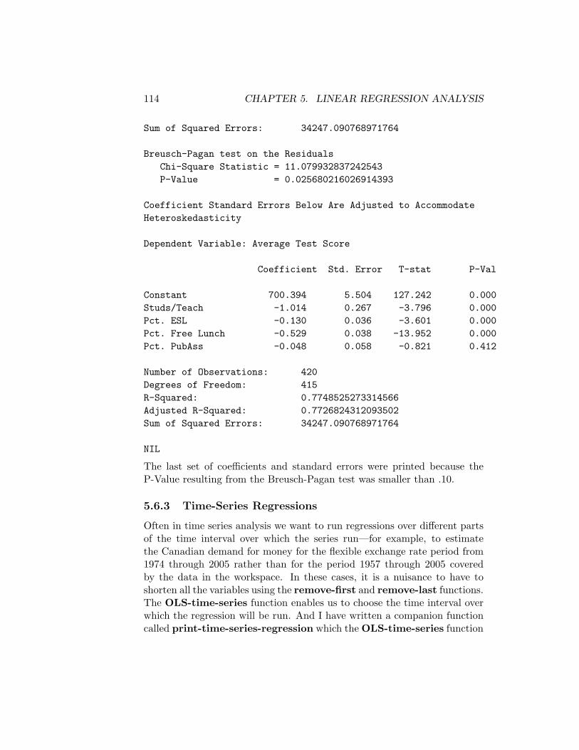
114 CHAPTER 5. LINEAR REGRESSION ANALYSIS
Sum of Squared Errors: 34247.090768971764
Breusch-Pagan test on the ResidualsChi-Square Statistic = 11.079932837242543P-Value = 0.025680216026914393
Coefficient Standard Errors Below Are Adjusted to AccommodateHeteroskedasticity
Dependent Variable: Average Test Score
Coefficient Std. Error T-stat P-Val
Constant 700.394 5.504 127.242 0.000Studs/Teach -1.014 0.267 -3.796 0.000Pct. ESL -0.130 0.036 -3.601 0.000Pct. Free Lunch -0.529 0.038 -13.952 0.000Pct. PubAss -0.048 0.058 -0.821 0.412
Number of Observations: 420Degrees of Freedom: 415R-Squared: 0.7748525273314566Adjusted R-Squared: 0.7726824312093502Sum of Squared Errors: 34247.090768971764
NIL
The last set of coefficients and standard errors were printed because theP-Value resulting from the Breusch-Pagan test was smaller than .10.
5.6.3 Time-Series Regressions
Often in time series analysis we want to run regressions over different partsof the time interval over which the series run—for example, to estimatethe Canadian demand for money for the flexible exchange rate period from1974 through 2005 rather than for the period 1957 through 2005 coveredby the data in the workspace. In these cases, it is a nuisance to have toshorten all the variables using the remove-first and remove-last functions.The OLS-time-series function enables us to choose the time interval overwhich the regression will be run. And I have written a companion functioncalled print-time-series-regression which the OLS-time-series function

5.6. SOME IMPROVED LINEAR REGRESSION FUNCTIONS 115
automatically calls when instructed to print the regression results. TheOLS-time-series function takes seven arguments in the following order.—the name of the dependent variable—a matrix of the independent variables, excluding the constant—the datelist to which all the time series being used conform—the date at which the regression is to begin—the date at which the regression is to end— 1 if a constant is to be included, 0 otherwise— 1 if the results are to be printed, 0 otherwiseThe function is used as follows, where the we first need to reset the Canadiandata.
> (load "addfuncs"); loading addfuncs.lspT> (load "camoinpr"); loading camoinpr.lspT> (seasdums-Q dates57 1)QD3> (def rm1ca (/ m1ca cpica))RM1CA> (def rgdpca (/ gdpsaca cpica))RGDPCA> (def rm1ca (base rm1ca dates57 1963.0 16))RM1CA> (def rgdpca (base rgdpca dates57 1963 16))RGDPCA> (def regressand "Log Real M1")REGRESSAND> (def regressors (list "Constant" "Interest Rate" "Log Real GDP" "QD1"))REGRESSORS> (def canreg (OLS-time-series (log rm1ca)(bind-columns cpaprqca (log rgdpca)QD1) dates57 1974.0 2005.75 1 1))
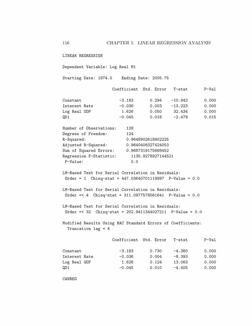
116 CHAPTER 5. LINEAR REGRESSION ANALYSIS
LINEAR REGRESSION
Dependent Variable: Log Real M1
Starting Date: 1974.0 Ending Date: 2005.75
Coefficient Std. Error T-stat P-Val
Constant -3.183 0.294 -10.842 0.000Interest Rate -0.036 0.003 -13.223 0.000Log Real GDP 1.626 0.050 32.434 0.000QD1 -0.045 0.018 -2.479 0.015
Number of Observations: 128Degrees of Freedom: 124R-Squared: 0.9648902618902225Adjusted R-Squared: 0.9640408327424053Sum of Squared Errors: 0.9687319175668452Regression F-Statistic: 1135.9278927144521P-Value: 0.0
LM-Based Test for Serial Correlation in Residuals:Order = 1 Chisq-stat = 447.03640701119997 P-Value = 0.0
LM-Based Test for Serial Correlation in Residuals:Order =< 4 Chisq-stat = 311.0977578561641 P-Value = 0.0
LM-Based Test for Serial Correlation in Residuals:Order =< 32 Chisq-stat = 202.9411344027211 P-Value = 0.0
Modified Results Using HAC Standard Errors of Coefficients:Truncation lag = 4
Coefficient Std. Error T-stat P-Val
Constant -3.183 0.730 -4.360 0.000Interest Rate -0.036 0.004 -8.393 0.000Log Real GDP 1.626 0.124 13.063 0.000QD1 -0.045 0.010 -4.405 0.000
CANREG

5.6. SOME IMPROVED LINEAR REGRESSION FUNCTIONS 117
Note that this function allows us to run a regression over any contigu-ous set of dates within the datelist dates57 to which the Canadian datawe loaded conforms. Obviously, the beginning and ending dates must bein the datelist and the beginning date must precede the ending date. Thefunction requires that the previously noted regressand and regressor ob-jects, which consist of the names assigned to the dependent and indepen-dent variables in the print-out, be in the workspace. In the above case wecalled the OLS-time-series function so that the regression-object it pro-duces will have the name CANREG, separate from the name LASTREG, whichwill be overwritten by regressions we subsequently choose to run. Both ob-jects were produced by the regression-model function (called within OLS-time-series) and are uncontaminated by HAC coefficient standard-errorcalculations. They are left in the workspace along with the list newdates,the datelist to which the regression conforms. Every object used in sub-sequent calculations regarding this regression must be obtained by sendinga message to canreg. The object LASTREG will be overwritten when thenext regression is run, as will any associated generically named object. TheLM serial correlation test is done for three different orders—1, .75T 1/3 andT/4, where the latter two expressions are rounded to the nearest integer.13
Rejection of the null-hypothesis of no serial correlation for the highest or-der combined with a failure to reject for the two lowest orders would be anindication that the HAC calculations above are insufficient, requiring fur-ther application of the LMSC-test function to identify the highest order ofautocorrelation and subsequent estimation using the OLS-basic functionwith that order imposed.
One can run a regression with the print argument set to 0, and thensubsequently call the print-time-series-regression function, which takesas its single argument the name of the regression-model object, to performall the tests for heteroskedasticity and autocorrelation and calculate theHAC standard-errors of the coefficients if heteroskedasticity and/or serialcorrelation cannot be rejected at the 10% level, and to print out the results.This latter function uses no variables already in the workspace other thanthe regression-model object it is given and regressand and regressors.
13The order T/4, appropriately rounded, is the maximum order conventionally used forthe LBQ statistic when testing for serial correlation in regression residuals. The order.75 T 1/3 is the guideline truncation parameter for HAC estimators suggested by Stock andWatson on page 504 of their Introduction to Econometrics.

118 CHAPTER 5. LINEAR REGRESSION ANALYSIS
5.6.4 Adjusting the Lengths of Time-Series and Setting upLagged Values
Another cause of complexity in time series analysis is the creation of laggedvalues of various series that one might want to include in a time seriesregression. Also, all series involved must be made to conform to the datelistspecified in the OLS-time-series function. My function set-time-series,which was introduced in section 6 of Chapter 2, simplifies these tasks. Thefunction takes five arguments:—the name of the list representing the series to be modified—the datelist to which the series conforms—the date at which the adjusted series is to begin—the date at which the adjusted series is to end—the number of lags of the series that are to be createdIf the number of lags created exceeds zero, the function creates an appro-priate block-lag matrix with smallest lags to the left and no current levelof the series included. Setting the number of lags at zero produces a listcontaining the date-adjusted unlagged version of the series specified. Thefunction leaves a list of lists called laglist in the workspace containing thecurrent series and all lags requested with the element number, starting atzero, giving the lag. To construct a matrix of selected lagged levels, one canextract the particular lags desired from laglist and bind them together,including the current level if desired, into an appropriately named matrix.All matrices of independent variables created in this way must be boundtogether using the bind-columns function for use as the appropriate argu-ment in the OLS-time-series function. For example, suppose we want towant to use the current level of the money supply along with a two quarterand a four quarter lag as independent variables in a regression. We wouldcreate the relevant matrix as follows.
(def tempm1mat (set-time-series m1ca dates57 1960.0 2005.75 4))(def m1ca (select laglist 0))(def m1ca-L2 (select laglist 2))(def m1ca-L4 (select laglist 4))(def m1mat (bind-columns m1ca m1ca-L2 m1ca-L4))
The calculations involving laglist must be done before the set-time-series function is called again because that object will be overwritten. Notealso that the above code overwrites the list m1ca with a shorter versionconforming to a datelist running from the first quarter of 1960 to the lastquarter of 2005. That datelist is called adjdates which is also left in theworkspace, and will be overwritten the next time the function is called.

Chapter 6
Regression Analysis of PanelData
A panel (or longitudinal) data set consists of observations of variables for agroup of entities for more than one period in time. Here, we will deal withpanel data sets structured in either of two ways:
Stacked Time-Series Stacked Cross-SectionsObs Ent Time Var1 Var2 Obs Ent Time Var1 Var21 1 1982 25 192 1 1 1982 25 1922 1 1983 31 161 2 2 1982 5 553 1 1984 18 89 3 1 1983 31 1614 2 1982 5 55 4 2 1983 21 245 2 1983 21 24 5 1 1984 18 896 2 1984 14 91 6 2 1984 14 91
As an example, we use a portion of the panel data set on traffic fatalitiesanalysed by Stock and Watson in Chapter 8 of their introductory book.This chapter is a useful read for someone trying to become familiar withpanel-data methods. These data are stacked time-series running annuallyfrom 1982 through 1988 and have been copied to the file fataldat.lsp.
> (load "addfuncs"); loading addfuncs.lspT> (load "fataldat"); loading fataldat.lspT
119

120 CHAPTER 6. REGRESSION ANALYSIS OF PANEL DATA
> (variables)(BEERTAX COMSERD ENTITY-FAT JAILD MLDA MRALL OBSNUM-FAT PERINCUNRATE VMILES YEAR-FAT)
The variables OBSNUM-FAT, ENTITY-FAT, and YEAR-FAT refer respectively tothe observation numbers, the entities (48 states, numbered 1 through 48)and the years (1982 through 1988). The suffix -FAT is added to the namesOBSNUM, ENTITY and YEAR to ensure that they will not be overwritten byfunctions that commonly use the latter object-names. The other variables,one observation per year per state, are
BEERTAX —Tax on a Case of BeerCOMSERD —Mandatory Community Service Sentence on ConvictionJAILD —Mandatory Jail Sentence on ConvictionMLDA —Minimum Legal Drinking AgePERINC —Real Per Capita IncomeUNRATE —Unemployment RateMRALL —Vehicle Fatality RateVMILES —Average Miles Driven per Driver
With the objective of determining whether an increase in the beer tax hasa negative effect on traffic fatalities, we start by regressing MRALL on BEERTAXusing our OLS-cross-section function after multiplying the fatality rateMRALL by 1000 so the regression coefficients will be big enough to show upon the print-out. In doing so, we rename that variable FATRATE.
> (first-five mrall)(2.1284E-4 2.3485E-4 2.3364E-4 2.1935E-4 2.6691E-4)> (def fatrate (* mrall 1000))FATRATE> (first-five fatrate)(2.1284 2.3485 2.3364 2.1935 2.6691)> (def regressand "Fatality Rate")REGRESSAND> (def regressors (list "Constant" "Beer Tax"))REGRESSORS> (def fatreg1 (OLS-cross-section fatrate (bind-columns beertax) 1))
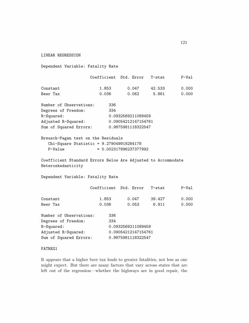
121
LINEAR REGRESSION
Dependent Variable: Fatality Rate
Coefficient Std. Error T-stat P-Val
Constant 1.853 0.047 42.533 0.000Beer Tax 0.036 0.062 5.861 0.000
Number of Observations: 336Degrees of Freedom: 334R-Squared: 0.0932569211089459Adjusted R-Squared: 0.09054212147154761Sum of Squared Errors: 0.9875981118322547
Breusch-Pagan test on the ResidualsChi-Square Statistic = 9.279049918284178P-Value = 0.002317896237377992
Coefficient Standard Errors Below Are Adjusted to AccommodateHeteroskedasticity
Dependent Variable: Fatality Rate
Coefficient Std. Error T-stat P-Val
Constant 1.853 0.047 39.427 0.000Beer Tax 0.036 0.053 6.911 0.000
Number of Observations: 336Degrees of Freedom: 334R-Squared: 0.0932569211089459Adjusted R-Squared: 0.09054212147154761Sum of Squared Errors: 0.9875981118322547
FATREG1
It appears that a higher beer tax leads to greater fatalities, not less as onemight expect. But there are many factors that vary across states that areleft out of the regression—whether the highways are in good repair, the

122 CHAPTER 6. REGRESSION ANALYSIS OF PANEL DATA
proportion of total driving that occurs in rural areas where traffic is lessdense, the social acceptability of drinking and driving, and so forth.
6.1 Differences Estimation
If we can assume that left out factors like the above remain constant overtime in individual states, a way to get around the missing variable problemis to compare the change in the fatality rate over time with the change inthe beer tax over time—factors remaining fixed over time in each state willcancel out. To do this, however, we have to extract and collect together allthe observations associated with individual years. We can do this using mypanel-collect-obsnums function. This function takes three arguments—in this case, the name of the time list (YEAR-FAT), the name of the entitylist (ENTITY-FAT) and the point in time for which we want to collect theobservation numbers.
> (def obslist-82 (panel-collect-obsnums year-fat entity-fat1982))OBSLIST-82> (def obslist-88 (panel-collect-obsnums year-fat entity-fat1988))OBSLIST-88> obslist-82(0 7 14 21 28 35 42 49 56 63 70 77 84 91 98 105 112 119 126 133 140147 154 161 168 175 182 189 196 203 210 217 224 231 238 245 252 259266 273 280 287 294 301 308 315 322 329)> obslist-88(6 13 20 27 34 41 48 55 62 69 76 83 90 97 104 111 118 125 132 139146 153 160 167 174 181 188 195 202 209 216 223 230 237 244 251 258265 272 279 286 293 300 307 314 321 328 335)
These two observation lists give the observation numbers in the panel asso-ciated with the respective years 1982 and 1988. We can now use them toselect the elements of each of the variables associated with the first and lastyears in the panel.
> (def fatrate-82 (select fatrate obslist-82))FATRATE-82> (def fatrate-88 (select fatrate obslist-88))FATRATE-88> (def beertax-82 (select beertax obslist-82))
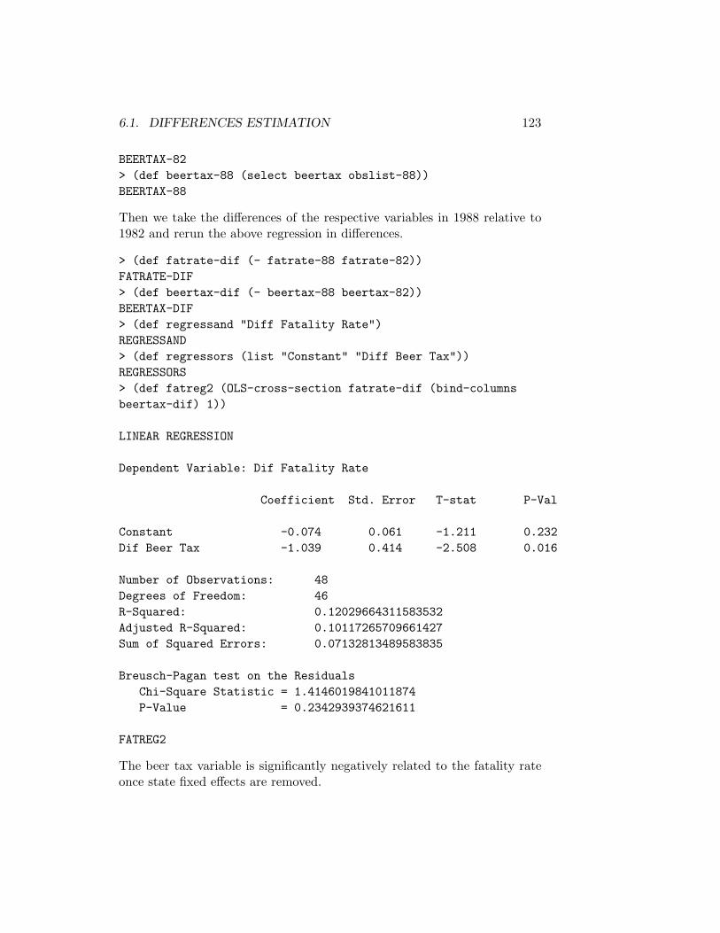
6.1. DIFFERENCES ESTIMATION 123
BEERTAX-82> (def beertax-88 (select beertax obslist-88))BEERTAX-88
Then we take the differences of the respective variables in 1988 relative to1982 and rerun the above regression in differences.
> (def fatrate-dif (- fatrate-88 fatrate-82))FATRATE-DIF> (def beertax-dif (- beertax-88 beertax-82))BEERTAX-DIF> (def regressand "Diff Fatality Rate")REGRESSAND> (def regressors (list "Constant" "Diff Beer Tax"))REGRESSORS> (def fatreg2 (OLS-cross-section fatrate-dif (bind-columnsbeertax-dif) 1))
LINEAR REGRESSION
Dependent Variable: Dif Fatality Rate
Coefficient Std. Error T-stat P-Val
Constant -0.074 0.061 -1.211 0.232Dif Beer Tax -1.039 0.414 -2.508 0.016
Number of Observations: 48Degrees of Freedom: 46R-Squared: 0.12029664311583532Adjusted R-Squared: 0.10117265709661427Sum of Squared Errors: 0.07132813489583835
Breusch-Pagan test on the ResidualsChi-Square Statistic = 1.4146019841011874P-Value = 0.2342939374621611
FATREG2
The beer tax variable is significantly negatively related to the fatality rateonce state fixed effects are removed.
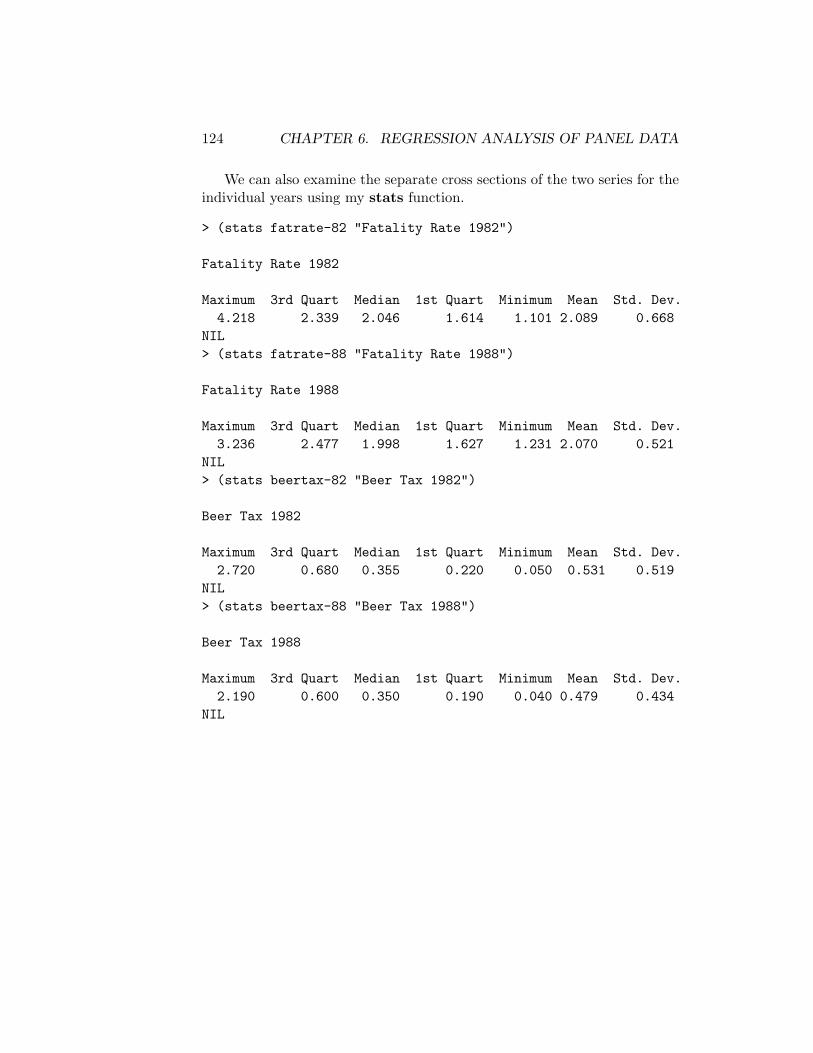
124 CHAPTER 6. REGRESSION ANALYSIS OF PANEL DATA
We can also examine the separate cross sections of the two series for theindividual years using my stats function.
> (stats fatrate-82 "Fatality Rate 1982")
Fatality Rate 1982
Maximum 3rd Quart Median 1st Quart Minimum Mean Std. Dev.4.218 2.339 2.046 1.614 1.101 2.089 0.668
NIL> (stats fatrate-88 "Fatality Rate 1988")
Fatality Rate 1988
Maximum 3rd Quart Median 1st Quart Minimum Mean Std. Dev.3.236 2.477 1.998 1.627 1.231 2.070 0.521
NIL> (stats beertax-82 "Beer Tax 1982")
Beer Tax 1982
Maximum 3rd Quart Median 1st Quart Minimum Mean Std. Dev.2.720 0.680 0.355 0.220 0.050 0.531 0.519
NIL> (stats beertax-88 "Beer Tax 1988")
Beer Tax 1988
Maximum 3rd Quart Median 1st Quart Minimum Mean Std. Dev.2.190 0.600 0.350 0.190 0.040 0.479 0.434
NIL

6.2. ENTITY DEMEANED FIXED EFFECTS REGRESSION 125
6.2 Entity Demeaned Fixed Effects Regression
An alternative way of handling the problem of state fixed effects that utilisesall years in the panel is to de-mean the data for each state—that is, to sub-tract from the level of every variable for each state the respective statemean. To do this I have written a function called panel-entity-demeanwhich takes two arguments—first the variable and second the entity-list(ENTITY-FAT). This function also requires that the panel data be organ-ised in stacked time-series form so that the observations for each entity arecontiguous.
> (def fatrate-dmn (panel-entity-demean fatrate entity-fat))FATRATE-DMN> (def beertax-dmn (panel-entity-demean beertax entity-fat))BEERTAX-DMN> (def regressand "Fatality Rate (All Variables are De-meaned)")REGRESSAND> (def regressors (list "Constant" "Beer Tax"))REGRESSORS> (def fatreg3 (OLS-cross-section fatrate-dmn (bind-columnsbeertax-dmn) 1))
LINEAR REGRESSION
Dependent Variable: Fatality Rate (All Variables are De-meaned)
Coefficient Std. Error T-stat P-Val
Constant 0.000 0.001 0.000 1.000Beer Tax -0.666 0.173 -3.849 0.000
Number of Observations: 336Degrees of Freedom: 334R-Squared: 0.04247439357535032Adjusted R-Squared: 0.03960755044234254Sum of Squared Errors: 0.10326636882938052
Breusch-Pagan test on the ResidualsChi-Square Statistic = 0.05941602778135291P-Value = 0.8074213242407234
FATREG3

126 CHAPTER 6. REGRESSION ANALYSIS OF PANEL DATA
Notice how we extended the definition of the regressand to include a state-ment that all variables are de-meaned—this was necessary because otherwisethe name of the beer tax variable would be too long and the presentationwould be messed up.
6.3 Using Fixed-Effects Dummy Variables
A third way of allowing for missing state fixed effects variables is to set updummy variables, one for each state in this case, that take a value of 1 forobservations pertaining to the entity or state in question and 0 for obser-vations pertaining to all other entities. To prevent perfect multicollinearity,we omit the dummy for either the first state or the last—the regression con-stant term becomes, in effect, the dummy for that particular entity and theother dummy variables measure the fixed effects for those entities relativeto that for the omitted entity. Further, we can also construct time-fixed-effects dummy variables, one for each unit of time in the sample, where eachof these dummies takes a value of 1 for the time-unit it pertains to and avalue of 0 for all other time-units. And again, we have to omit the timedummy of one of the time-units, usually the first or the last, to preventperfect multicollinearity—all the remaining dummies measure the effect oftheir particular time-units relative to the omitted time-unit, whose effectis embedded in the constant term along with that of the missing entity-dummy. Just as the entity-fixed-effect dummies capture the effects of miss-ing variables that vary across entities but are constant through time, thetime-fixed-effect dummies capture the effects of missing variables that varythrough time but are constant across entities.
We can set up the fixed-effects dummies using the panel-set-fixed-effects function I wrote for the purpose. This function takes as its singleargument either the entity list (ENTITY-FAT) or the time list (YEAR-FAT).Both of these lists must take the form of contiguous integer units startingwith 1. The function returns a matrix containing fixed-effects dummies forall entities or time-fixed-effects dummies for all units of time. We then haveto delete either the first or the last column of each of these matrices.
> (def efemat (panel-set-fixed-effects entity-fat))EFEMAT> (def year-units (- year-fat 1981))YEAR-UNITS> (def tfemat (panel-set-fixed-effects year-units))TFEMAT

6.3. USING FIXED-EFFECTS DUMMY VARIABLES 127
> (def efemat (remove-first-columns 1 efemat))EFRMAT> (def tfemat (remove-first-columns 1 tfemat))TFEMAT
For doing regression analyses of panel data with dummy variables forentity and time fixed effects I have written the OLS-panel function. Thisfunction takes five arguments—in order, the list representing the dependentvariable, a matrix of independent variables excluding fixed-effects dummies,the matrix of entity fixed-effects dummy variables, the matrix of time-fixed-effects dummy variables, and the number 1 if a constant is to be included or 0otherwise. The function performs four sets of OLS-regression calculations—the first including both entity and time fixed-effects dummies, the secondincluding only time fixed effects, the third including only entity fixed effects,and the final one including no fixed effects at all.
We now redo the above regression analysis using the OLS-panel func-tion.
> (def regressand "Fatality Rate")REGRESSAND(def regressors (list "Constant" "Beer Tax"))REGRESSORS> (OLS-panel fatrate (bind-columns beertax) efemat tfemat 1)
LINEAR REGRESSION WITH ENTITY AND TIME FIXED EFFECTS
Dependent Variable: Fatality Rate
Coefficient Std. Error T-stat P-Val
Constant 3.536 0.331 10.691 0.000Beer Tax -0.655 0.196 -3.336 0.001
Entity Fixed Effects:F-statistic = 53.32628637864364P-Value = 0.0
Time Fixed Effects:F-statistic = 2.0268785384373054P-Value = 0.06219892621491452
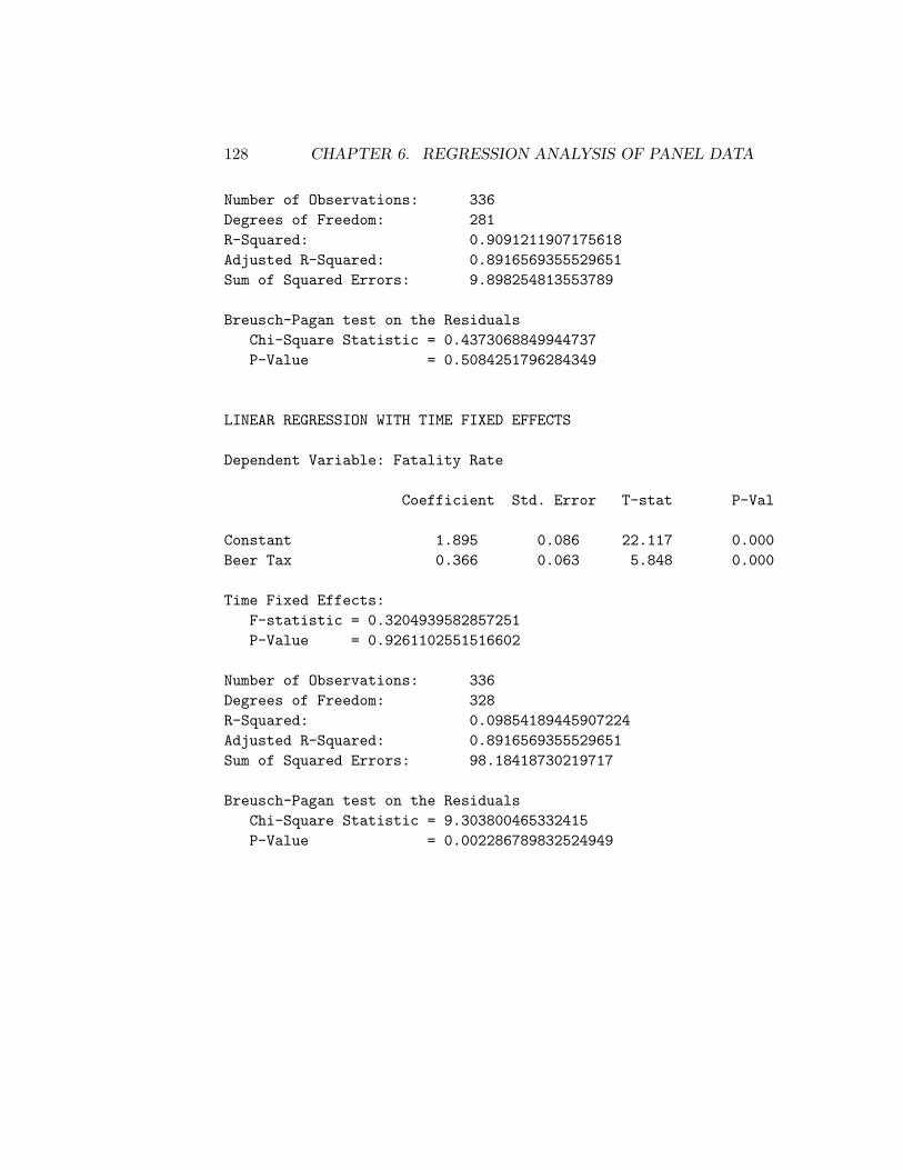
128 CHAPTER 6. REGRESSION ANALYSIS OF PANEL DATA
Number of Observations: 336Degrees of Freedom: 281R-Squared: 0.9091211907175618Adjusted R-Squared: 0.8916569355529651Sum of Squared Errors: 9.898254813553789
Breusch-Pagan test on the ResidualsChi-Square Statistic = 0.4373068849944737P-Value = 0.5084251796284349
LINEAR REGRESSION WITH TIME FIXED EFFECTS
Dependent Variable: Fatality Rate
Coefficient Std. Error T-stat P-Val
Constant 1.895 0.086 22.117 0.000Beer Tax 0.366 0.063 5.848 0.000
Time Fixed Effects:F-statistic = 0.3204939582857251P-Value = 0.9261102551516602
Number of Observations: 336Degrees of Freedom: 328R-Squared: 0.09854189445907224Adjusted R-Squared: 0.8916569355529651Sum of Squared Errors: 98.18418730219717
Breusch-Pagan test on the ResidualsChi-Square Statistic = 9.303800465332415P-Value = 0.002286789832524949
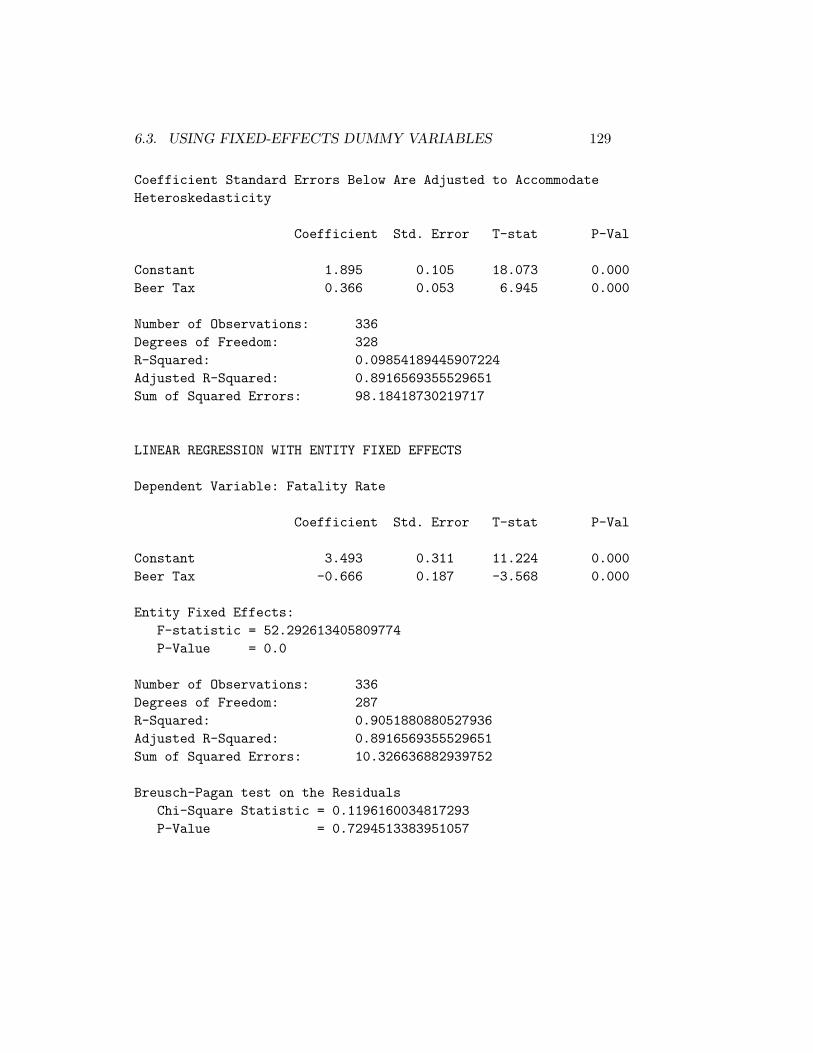
6.3. USING FIXED-EFFECTS DUMMY VARIABLES 129
Coefficient Standard Errors Below Are Adjusted to AccommodateHeteroskedasticity
Coefficient Std. Error T-stat P-Val
Constant 1.895 0.105 18.073 0.000Beer Tax 0.366 0.053 6.945 0.000
Number of Observations: 336Degrees of Freedom: 328R-Squared: 0.09854189445907224Adjusted R-Squared: 0.8916569355529651Sum of Squared Errors: 98.18418730219717
LINEAR REGRESSION WITH ENTITY FIXED EFFECTS
Dependent Variable: Fatality Rate
Coefficient Std. Error T-stat P-Val
Constant 3.493 0.311 11.224 0.000Beer Tax -0.666 0.187 -3.568 0.000
Entity Fixed Effects:F-statistic = 52.292613405809774P-Value = 0.0
Number of Observations: 336Degrees of Freedom: 287R-Squared: 0.9051880880527936Adjusted R-Squared: 0.8916569355529651Sum of Squared Errors: 10.326636882939752
Breusch-Pagan test on the ResidualsChi-Square Statistic = 0.1196160034817293P-Value = 0.7294513383951057
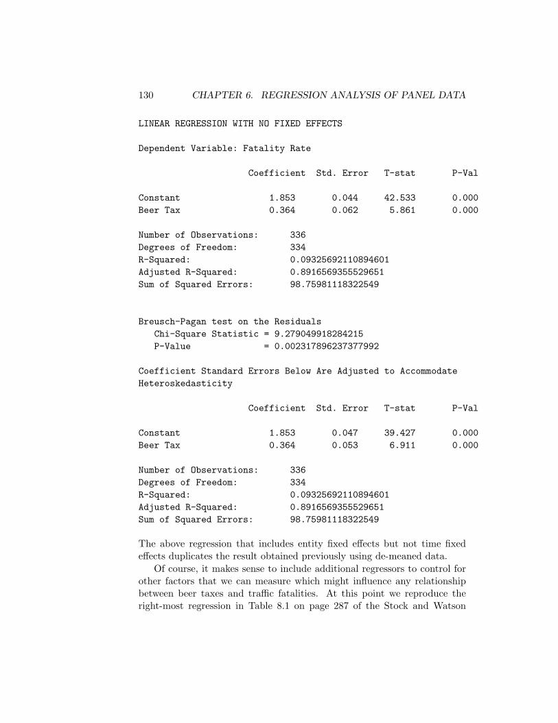
130 CHAPTER 6. REGRESSION ANALYSIS OF PANEL DATA
LINEAR REGRESSION WITH NO FIXED EFFECTS
Dependent Variable: Fatality Rate
Coefficient Std. Error T-stat P-Val
Constant 1.853 0.044 42.533 0.000Beer Tax 0.364 0.062 5.861 0.000
Number of Observations: 336Degrees of Freedom: 334R-Squared: 0.09325692110894601Adjusted R-Squared: 0.8916569355529651Sum of Squared Errors: 98.75981118322549
Breusch-Pagan test on the ResidualsChi-Square Statistic = 9.279049918284215P-Value = 0.002317896237377992
Coefficient Standard Errors Below Are Adjusted to AccommodateHeteroskedasticity
Coefficient Std. Error T-stat P-Val
Constant 1.853 0.047 39.427 0.000Beer Tax 0.364 0.053 6.911 0.000
Number of Observations: 336Degrees of Freedom: 334R-Squared: 0.09325692110894601Adjusted R-Squared: 0.8916569355529651Sum of Squared Errors: 98.75981118322549
The above regression that includes entity fixed effects but not time fixedeffects duplicates the result obtained previously using de-meaned data.
Of course, it makes sense to include additional regressors to control forother factors that we can measure which might influence any relationshipbetween beer taxes and traffic fatalities. At this point we reproduce theright-most regression in Table 8.1 on page 287 of the Stock and Watson
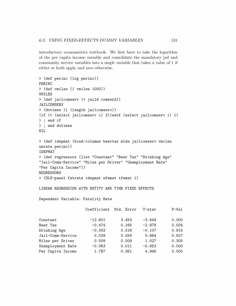
6.3. USING FIXED-EFFECTS DUMMY VARIABLES 131
introductory econometrics textbook. We first have to take the logarithmof the per capita income variable and consolidate the mandatory jail andcommunity service variables into a single variable that takes a value of 1 ifeither or both apply and zero otherwise.
> (def perinc (log perinc))PERINC> (def vmiles (/ vmiles 1000))VMILES> (def jailcomserv (+ jaild comserd))JAILCOMSERV> (dotimes (i (length jailcomserv))(if (= (select jailcomserv i) 2)(setf (select jailcomserv i) 1)) ; end if) ; end dotimesNIL
> (def idepmat (bind-columns beertax mlda jailcomserv vmilesunrate perinc))IDEPMAT> (def regressors (list "Constant" "Beer Tax" "Drinking Age""Jail-Comm-Service" "Miles per Driver" "Unemployment Rate""Per Capita Income"))REGRESSORS> (OLS-panel fatrate idepmat efemat tfemat 1)
LINEAR REGRESSION WITH ENTITY AND TIME FIXED EFFECTS
Dependent Variable: Fatality Rate
Coefficient Std. Error T-stat P-Val
Constant -12.601 3.453 -3.649 0.000Beer Tax -0.474 0.165 -2.878 0.004Drinking Age -0.002 0.018 -0.107 0.915Jail-Comm-Service 0.039 0.059 0.664 0.507Miles per Driver 0.009 0.009 1.027 0.305Unemployment Rate -0.063 0.011 -5.653 0.000Per Capita Income 1.787 0.361 4.946 0.000

132 CHAPTER 6. REGRESSION ANALYSIS OF PANEL DATA
Entity Fixed Effects:F-statistic = 47.635527799478346P-Value = 0.0
Time Fixed Effects:F-statistic = 19.548913853023127P-Value = 0.0
Number of Observations: 336Degrees of Freedom: 276R-Squared: 0.9393650302557469Adjusted R-Squared: 0.9264032070133159Sum of Squared Errors: 6.604184032335501
Breusch-Pagan test on the ResidualsChi-Square Statistic = 11.632497706504546P-Value = 0.07068778606103288
Coefficient Standard Errors Below Are Adjusted to AccommodateHeteroskedasticity
Coefficient Std. Error T-stat P-Val
Constant -12.601 3.941 -3.197 0.002Beer Tax -0.474 0.198 -2.389 0.018Drinking Age -0.002 0.016 -0.121 0.904Jail-Comm-Service 0.039 0.076 0.518 0.605Miles per Driver 0.009 0.007 1.260 0.209Unemployment Rate -0.063 0.010 -5.965 0.000Per Capita Income 1.787 0.410 4.358 0.000
Number of Observations: 336Degrees of Freedom: 276R-Squared: 0.9393650302557469Adjusted R-Squared: 0.9264032070133159Sum of Squared Errors: 6.604184032335501

6.3. USING FIXED-EFFECTS DUMMY VARIABLES 133
LINEAR REGRESSION WITH TIME FIXED EFFECTS
Dependent Variable: Fatality Rate
Coefficient Std. Error T-stat P-Val
Constant 15.880 2.177 7.294 0.000Beer Tax 0.102 0.056 1.835 0.067Drinking Age -0.011 0.029 -0.386 0.700Jail-Comm-Service 0.274 0.052 5.268 0.000Miles per Driver 0.129 0.018 7.245 0.000Unemployment Rate 0.001 0.014 0.099 0.921Per Capita Income -1.546 0.210 -7.366 0.000
Time Fixed Effects:F-statistic = 0.8267459319549197P-Value = 0.5498357636865194
Number of Observations: 336Degrees of Freedom: 323R-Squared: 0.44750342524478237Adjusted R-Squared: 0.9264032070133159Sum of Squared Errors: 60.17631528981331
Breusch-Pagan test on the ResidualsChi-Square Statistic = 126.5800386028212P-Value = 0.0
Coefficient Standard Errors Below Are Adjusted to AccommodateHeteroskedasticity
Coefficient Std. Error T-stat P-Val
Constant 15.880 2.782 5.708 0.000Beer Tax 0.102 0.050 2.025 0.044Drinking Age -0.011 0.026 -0.424 0.672Jail-Comm-Service 0.274 0.058 4.715 0.000Miles per Driver 0.129 0.076 1.701 0.090Unemployment Rate 0.001 0.015 0.088 0.930Per Capita Income -1.546 0.239 -6.456 0.000
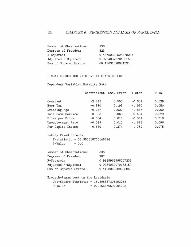
134 CHAPTER 6. REGRESSION ANALYSIS OF PANEL DATA
Number of Observations: 336Degrees of Freedom: 323R-Squared: 0.44750342524478237Adjusted R-Squared: 0.9264032070133159Sum of Squared Errors: 60.17631528981331
LINEAR REGRESSION WITH ENTITY FIXED EFFECTS
Dependent Variable: Fatality Rate
Coefficient Std. Error T-stat P-Val
Constant -2.243 3.555 -0.631 0.529Beer Tax -0.380 0.193 -1.970 0.050Drinking Age -0.037 0.020 -1.887 0.060Jail-Comm-Service -0.033 0.069 -0.484 0.629Miles per Driver -0.004 0.010 -0.361 0.718Unemployment Rate -0.019 0.012 -1.672 0.096Per Capita Income 0.669 0.374 1.789 0.075
Entity Fixed Effects:F-statistic = 32.955518766148494P-Value = 0.0
Number of Observations: 336Degrees of Freedom: 282R-Squared: 0.9135965998207236Adjusted R-Squared: 0.9264032070133159Sum of Squared Errors: 9.410806308805885
Breusch-Pagan test on the ResidualsChi-Square Statistic = 15.508837306993268P-Value = 0.0166476692094093
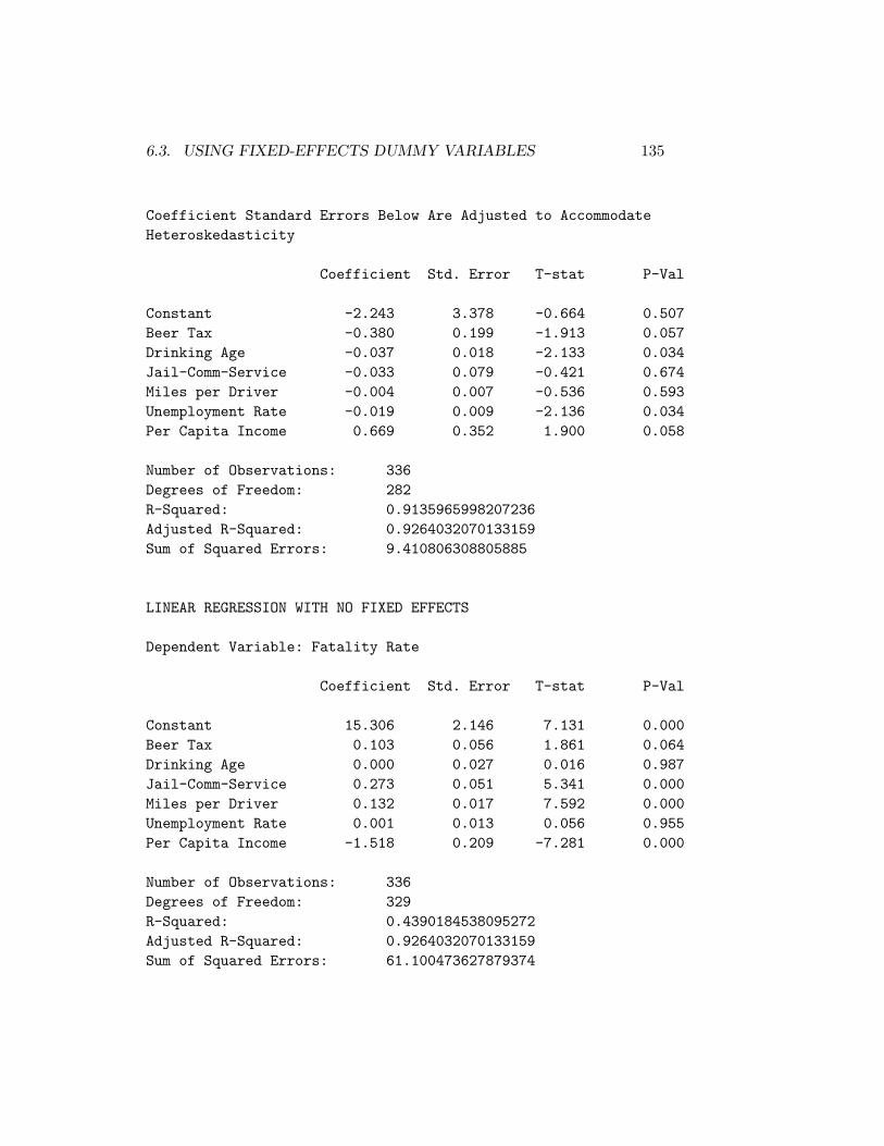
6.3. USING FIXED-EFFECTS DUMMY VARIABLES 135
Coefficient Standard Errors Below Are Adjusted to AccommodateHeteroskedasticity
Coefficient Std. Error T-stat P-Val
Constant -2.243 3.378 -0.664 0.507Beer Tax -0.380 0.199 -1.913 0.057Drinking Age -0.037 0.018 -2.133 0.034Jail-Comm-Service -0.033 0.079 -0.421 0.674Miles per Driver -0.004 0.007 -0.536 0.593Unemployment Rate -0.019 0.009 -2.136 0.034Per Capita Income 0.669 0.352 1.900 0.058
Number of Observations: 336Degrees of Freedom: 282R-Squared: 0.9135965998207236Adjusted R-Squared: 0.9264032070133159Sum of Squared Errors: 9.410806308805885
LINEAR REGRESSION WITH NO FIXED EFFECTS
Dependent Variable: Fatality Rate
Coefficient Std. Error T-stat P-Val
Constant 15.306 2.146 7.131 0.000Beer Tax 0.103 0.056 1.861 0.064Drinking Age 0.000 0.027 0.016 0.987Jail-Comm-Service 0.273 0.051 5.341 0.000Miles per Driver 0.132 0.017 7.592 0.000Unemployment Rate 0.001 0.013 0.056 0.955Per Capita Income -1.518 0.209 -7.281 0.000
Number of Observations: 336Degrees of Freedom: 329R-Squared: 0.4390184538095272Adjusted R-Squared: 0.9264032070133159Sum of Squared Errors: 61.100473627879374
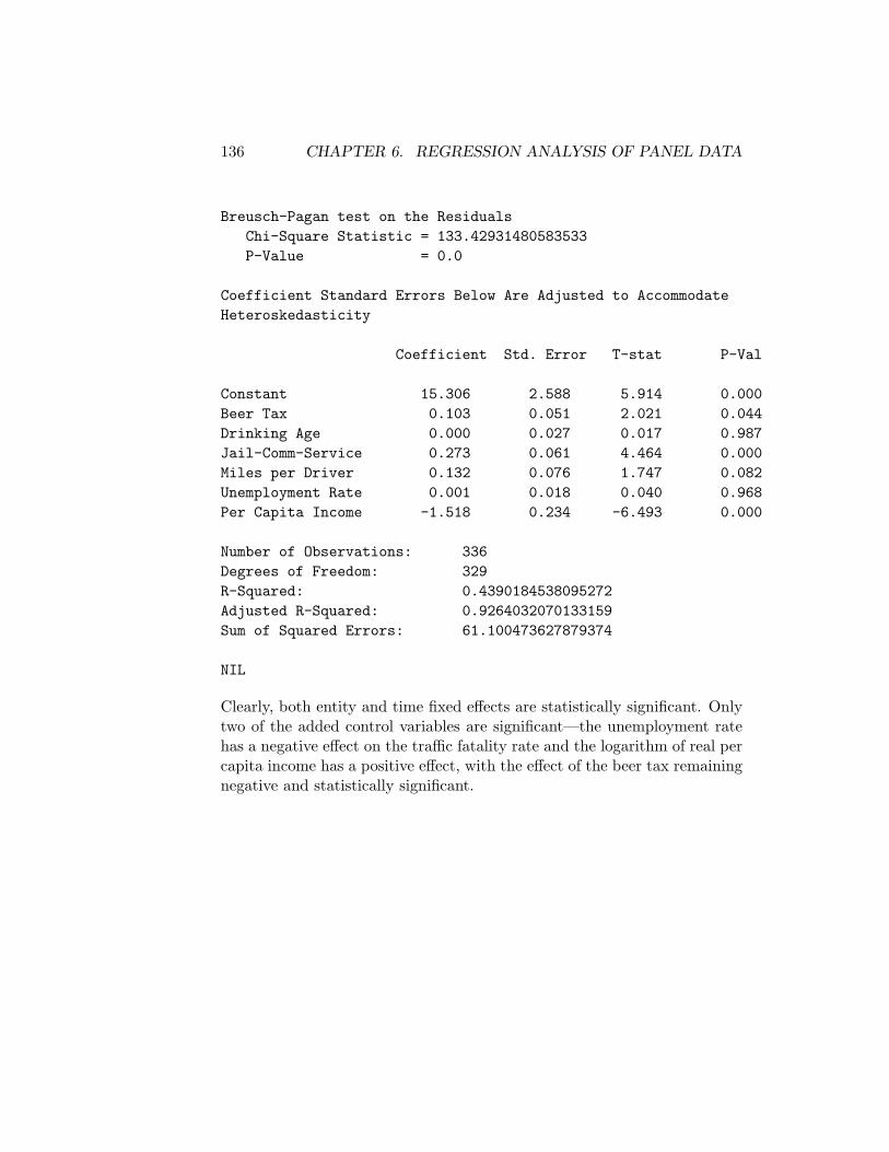
136 CHAPTER 6. REGRESSION ANALYSIS OF PANEL DATA
Breusch-Pagan test on the ResidualsChi-Square Statistic = 133.42931480583533P-Value = 0.0
Coefficient Standard Errors Below Are Adjusted to AccommodateHeteroskedasticity
Coefficient Std. Error T-stat P-Val
Constant 15.306 2.588 5.914 0.000Beer Tax 0.103 0.051 2.021 0.044Drinking Age 0.000 0.027 0.017 0.987Jail-Comm-Service 0.273 0.061 4.464 0.000Miles per Driver 0.132 0.076 1.747 0.082Unemployment Rate 0.001 0.018 0.040 0.968Per Capita Income -1.518 0.234 -6.493 0.000
Number of Observations: 336Degrees of Freedom: 329R-Squared: 0.4390184538095272Adjusted R-Squared: 0.9264032070133159Sum of Squared Errors: 61.100473627879374
NIL
Clearly, both entity and time fixed effects are statistically significant. Onlytwo of the added control variables are significant—the unemployment ratehas a negative effect on the traffic fatality rate and the logarithm of real percapita income has a positive effect, with the effect of the beer tax remainingnegative and statistically significant.
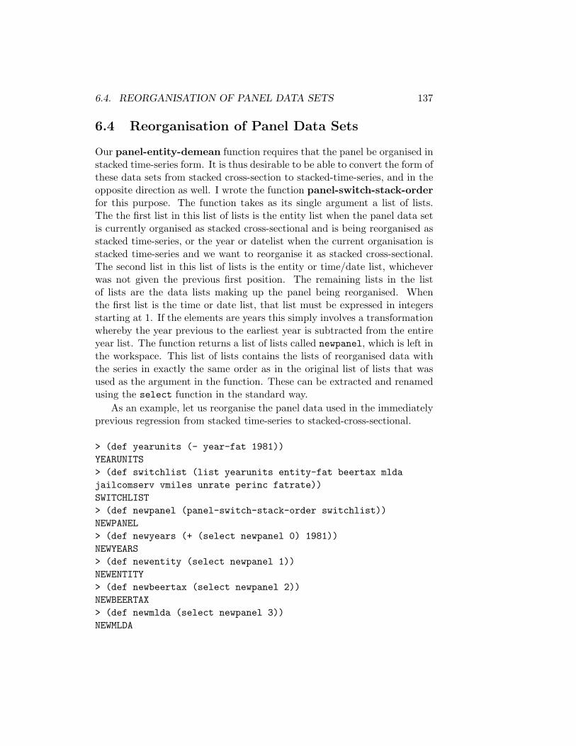
6.4. REORGANISATION OF PANEL DATA SETS 137
6.4 Reorganisation of Panel Data Sets
Our panel-entity-demean function requires that the panel be organised instacked time-series form. It is thus desirable to be able to convert the form ofthese data sets from stacked cross-section to stacked-time-series, and in theopposite direction as well. I wrote the function panel-switch-stack-orderfor this purpose. The function takes as its single argument a list of lists.The the first list in this list of lists is the entity list when the panel data setis currently organised as stacked cross-sectional and is being reorganised asstacked time-series, or the year or datelist when the current organisation isstacked time-series and we want to reorganise it as stacked cross-sectional.The second list in this list of lists is the entity or time/date list, whicheverwas not given the previous first position. The remaining lists in the listof lists are the data lists making up the panel being reorganised. Whenthe first list is the time or date list, that list must be expressed in integersstarting at 1. If the elements are years this simply involves a transformationwhereby the year previous to the earliest year is subtracted from the entireyear list. The function returns a list of lists called newpanel, which is left inthe workspace. This list of lists contains the lists of reorganised data withthe series in exactly the same order as in the original list of lists that wasused as the argument in the function. These can be extracted and renamedusing the select function in the standard way.
As an example, let us reorganise the panel data used in the immediatelyprevious regression from stacked time-series to stacked-cross-sectional.
> (def yearunits (- year-fat 1981))YEARUNITS> (def switchlist (list yearunits entity-fat beertax mldajailcomserv vmiles unrate perinc fatrate))SWITCHLIST> (def newpanel (panel-switch-stack-order switchlist))NEWPANEL> (def newyears (+ (select newpanel 0) 1981))NEWYEARS> (def newentity (select newpanel 1))NEWENTITY> (def newbeertax (select newpanel 2))NEWBEERTAX> (def newmlda (select newpanel 3))NEWMLDA
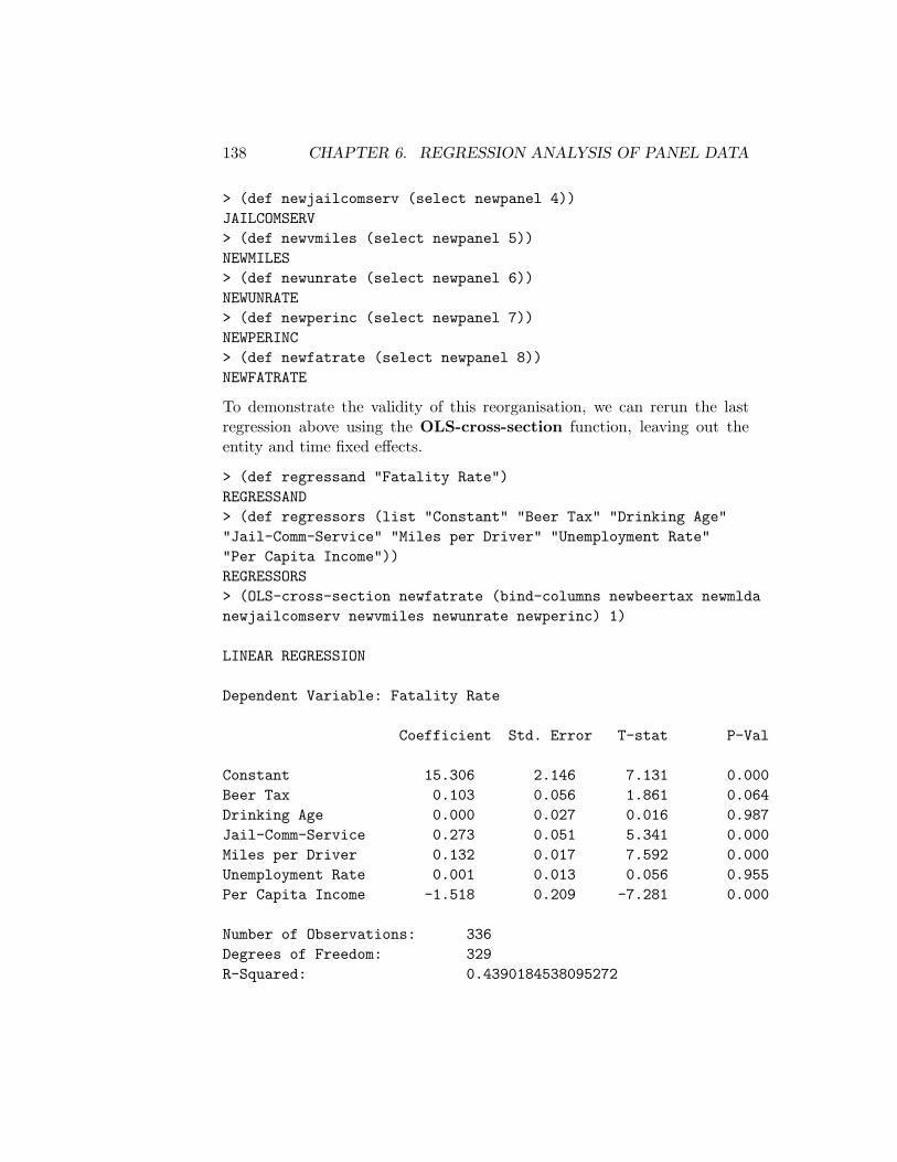
138 CHAPTER 6. REGRESSION ANALYSIS OF PANEL DATA
> (def newjailcomserv (select newpanel 4))JAILCOMSERV> (def newvmiles (select newpanel 5))NEWMILES> (def newunrate (select newpanel 6))NEWUNRATE> (def newperinc (select newpanel 7))NEWPERINC> (def newfatrate (select newpanel 8))NEWFATRATE
To demonstrate the validity of this reorganisation, we can rerun the lastregression above using the OLS-cross-section function, leaving out theentity and time fixed effects.
> (def regressand "Fatality Rate")REGRESSAND> (def regressors (list "Constant" "Beer Tax" "Drinking Age""Jail-Comm-Service" "Miles per Driver" "Unemployment Rate""Per Capita Income"))REGRESSORS> (OLS-cross-section newfatrate (bind-columns newbeertax newmldanewjailcomserv newvmiles newunrate newperinc) 1)
LINEAR REGRESSION
Dependent Variable: Fatality Rate
Coefficient Std. Error T-stat P-Val
Constant 15.306 2.146 7.131 0.000Beer Tax 0.103 0.056 1.861 0.064Drinking Age 0.000 0.027 0.016 0.987Jail-Comm-Service 0.273 0.051 5.341 0.000Miles per Driver 0.132 0.017 7.592 0.000Unemployment Rate 0.001 0.013 0.056 0.955Per Capita Income -1.518 0.209 -7.281 0.000
Number of Observations: 336Degrees of Freedom: 329R-Squared: 0.4390184538095272

6.4. REORGANISATION OF PANEL DATA SETS 139
Adjusted R-Squared: 0.4287877873136523Sum of Squared Errors: 61.100473627879325
Breusch-Pagan test on the ResidualsChi-Square Statistic = 133.42931480583323P-Value = 0.0
Coefficient Standard Errors Below Are Adjusted to AccommodateHeteroskedasticity
Dependent Variable: Fatality Rate
Coefficient Std. Error T-stat P-Val
Constant 15.306 2.588 5.914 0.000Beer Tax 0.103 0.051 2.021 0.044Drinking Age 0.000 0.027 0.017 0.987Jail-Comm-Service 0.273 0.061 4.464 0.000Miles per Driver 0.132 0.076 1.747 0.082Unemployment Rate 0.001 0.018 0.040 0.968Per Capita Income -1.518 0.234 -6.493 0.000
Number of Observations: 336Degrees of Freedom: 329R-Squared: 0.4390184538095272Adjusted R-Squared: 0.4287877873136523Sum of Squared Errors: 61.100473627879325
These regression results are identical with the previous ones that incorpo-rated neither entity nor time fixed effects.
When reorganising the panel from stacked cross-sectional to stackedtime-series it is not necessary to transform the year or date variable intointeger units that start at 1. In that case the year list enters the list of liststhat becomes the argument in the panel-switch-stack-order function inthe second position with the entity list taking first position.

140 CHAPTER 6. REGRESSION ANALYSIS OF PANEL DATA
Chapter 7
Instrumental VariablesRegression
A major problem arises in regression analysis when the error term is corre-lated with one or more of the independent variables. This can occur becausea variable that is correlated with these independent variables is left out of theregression. It also occurs when there is simultaneous causality—for example,left-out factors may shift the demand curve, resulting in shifts in the priceand or quantity as a result of movements along the supply curve. This willlead to correlation between the error term and whichever of price or quantityis being used as the independent variable in estimating the demand curve.The obvious remedy of including the left-out variable in the regression maynot be available because of lack of data. Independent variables that are cor-related with the error term in the equation are called endogenous variablesand those uncorrelated with the error term are called exogenous.
Under these circumstances an instrumental variables approach may beuseful. An excellent introduction to the basics of this topic is Chapter 10of the Stock and Watson introductory econometrics book, from which datasets are used in the exposition here. The basic idea is to find variables thatare correlated with the endogenous independent variable but not the errorterm, and use them as ‘instruments’ to cleanse the endogenous variable ofits correlation with the error term. To be useful, an instrumental variablemust satisfy two conditions: a) it must be relevant—that is, correlated withthe endogenous variable, and b) it must be exogenous—that is, uncorrelatedwith the error term.
141

142 CHAPTER 7. INSTRUMENTAL VARIABLES REGRESSION
7.1 Two-Stage Least Squares
The usual approach to instrumental variable estimation proceeds, using OLSmethods, in two stages—hence its name, two-stage least squares. The firststage simply involves regressing each endogenous variable in one’s ideal basicestimating equation (the equation one would run if there was no correlationof the independent variables with the error term) on one or more instru-mental variables together with all exogenous variables that would ordinarilyappear in that ideal equation, and then extracting the respective series offitted values. These fitted values have the property that they are inde-pendent of the residuals of the first-stage regression but correlated with theendogenous variable in question (if the instruments are relevant). Hopefully,they should thereby be purged of any correlation with the factors that willdetermine the residuals of the ideal basic estimating equation. The secondstage then simply applies OLS to this ideal equation where the endogenousvariables are replaced by their fitted values from the first-stage regressions.The coefficients of the fitted series should be free of the bias that would bepresent if the actual series were used in their place.
Since the purpose is to obtain appropriate fitted values of the endogenousvariables, the first-stage regression can best be run using our OLS-basicfunction with the right-most argument set to -1 to impose the assumptionthat the residuals are homogeneous. It is important that the instrumentsbe strongly related to the endogenous regressor being used as the dependentvariable in the first stage—this requires that they be statistically significant.A useful rule-of-thumb when there is a single endogenous regressor is thatthe first-stage F-statistic must exceed 10.
As an example, we can use some data on the U.S. commercial bank-loan market from G. S. Maddala’s introductory econometrics text.1 The filecontaining the data is loandata.lsp. The task is to measure the supplyand demand elasticities in that market.2
> (load "addfuncs"); loading addfuncs.lspT> (load "loandata"); loading loandata.lspT
1G. S. Maddala, Introduction to Econometrics, MacMillan, 1988.2This econometric exercise should not be taken seriously as a test of economic theory
because the data are for a short period many years ago.

7.1. TWO-STAGE LEAST SQUARES 143
> (variables)(CBNDRATE DATE7984 INDPROD PRIMRATE QLOANS TBRATE TOTBDEP)
The series run from January 1979 through December 1984 and can be de-scribed as follows:
QLOANS —Quantity of Commercial Loans Made by BanksPRIMRATE —Bank’s Prime Rate on Commercial LoansCBNDRATE —Interest Rate on Corporate BondsTBRATE —30-Day Treasury Bill RateINDPROD —Industrial ProductionTOTDEP —Total Bank Deposits
Appropriate structural equations representing the demand and supplyof commercial bank loans are:
Demand
QLOANS = β0 + β1 PRIMRATE + β2 CBNDRATE + β3 INDPROD
Supply
QLOANS = δ0 + δ1 PRIMRATE + δ2 TBRATE + δ3 TOTDEP
where β1 and δ2 are negative and all the other coefficients are positive.This says that banks will expand their supply of loans in response to ahigher prime rate, greater deposits, and a lower rate of return on alternativeinvestments in treasury bills, and that commercial enterprises will increasetheir demand for loans in response to a fall in the prime rate, a rise inthe cost of funding through corporate bond issues and an increase in theiroutput.
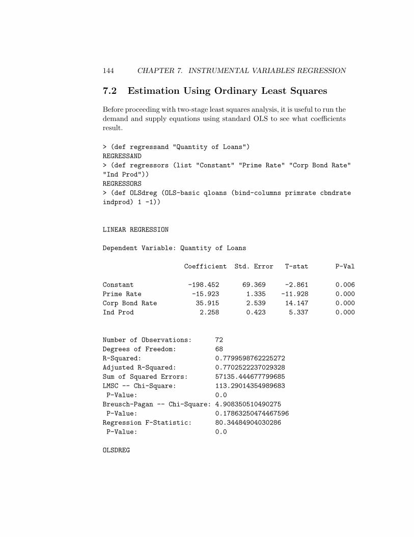
144 CHAPTER 7. INSTRUMENTAL VARIABLES REGRESSION
7.2 Estimation Using Ordinary Least Squares
Before proceeding with two-stage least squares analysis, it is useful to run thedemand and supply equations using standard OLS to see what coefficientsresult.
> (def regressand "Quantity of Loans")REGRESSAND> (def regressors (list "Constant" "Prime Rate" "Corp Bond Rate""Ind Prod"))REGRESSORS> (def OLSdreg (OLS-basic qloans (bind-columns primrate cbndrateindprod) 1 -1))
LINEAR REGRESSION
Dependent Variable: Quantity of Loans
Coefficient Std. Error T-stat P-Val
Constant -198.452 69.369 -2.861 0.006Prime Rate -15.923 1.335 -11.928 0.000Corp Bond Rate 35.915 2.539 14.147 0.000Ind Prod 2.258 0.423 5.337 0.000
Number of Observations: 72Degrees of Freedom: 68R-Squared: 0.7799598762225272Adjusted R-Squared: 0.7702522237029328Sum of Squared Errors: 57135.444677799685LMSC -- Chi-Square: 113.29014354989683P-Value: 0.0Breusch-Pagan -- Chi-Square: 4.908350510490275P-Value: 0.17863250474467596Regression F-Statistic: 80.34484904030286P-Value: 0.0
OLSDREG

7.2. ESTIMATION USING ORDINARY LEAST SQUARES 145
> (def regressors (list "Constant" "Prime Rate" "T-Bill Rate""Bank Deposits"))REGRESSORS> (def OLSsreg (OLS-basic qloans (bind-columns primrate tbratetotbdep) 1 -1))
LINEAR REGRESSION
Dependent Variable: Quantity of Loans
Coefficient Std. Error T-stat P-Val
Constant -77.469 11.234 -6.896 0.000Prime Rate 2.424 0.828 2.927 0.005T-Bill Rate -1.903 1.071 -1.777 0.080Bank Deposits 0.332 0.006 51.318 0.000
Number of Observations: 72Degrees of Freedom: 68R-Squared: 0.9767416046419778Adjusted R-Squared: 0.975715498964418Sum of Squared Errors: 6039.256561301388LMSC -- Chi-Square: 80.02576052366551P-Value: 0.0
Breusch-Pagan -- Chi-Square: 6.327661775518827P-Value: 0.09671258232287316
Regression F-Statistic: 951.89182362267P-Value: 0.0
OLSSREG
The variables have the expected signs since CBNDRATE and INDPROD stabilisethe demand curve and TBRATE and TOTBDEP stabilise the supply curve so thatchanges in PRIMRATE trace out estimated curves with the correctly signedslopes. Of course, these slope coefficients are biased because of missingfactors affecting the supply and demand curves.

146 CHAPTER 7. INSTRUMENTAL VARIABLES REGRESSION
7.3 First Stage TSLS Estimation
In the first stage of our two-stage analysis, it makes sense to use CBNDRATEand INDPROD as instruments for the supply equation and TBRATE and TOTBDEPas instruments for the demand equation because they obviously are relatedto PRIMRATE and their inclusion strips the fitted PRIMRATE series of corre-lation with the portions of the error terms they are responsible for in therespective supply and demand equations. Since the independent variablesin the first stage are the instruments plus the exogenous variables, we have asingle first-stage regression that determines the fitted values of PRIMRATE toinclude, in place of the actual PRIMRATE series, in both second-stage equa-tions.
> (def regressand "Prime Rate")REGRESSAND> (def regressors (list "Constant" "Corp Bond Rate" "Ind Prod""T-Bill Rate" "Bank Deposits"))REGRESSORS> (def tslsfsreg (OLS-basic primrate (bind-columns cbndrateindprod tbrate totbdep) 1 -1))
LINEAR REGRESSION
Dependent Variable: Prime Rate
Coefficient Std. Error T-stat P-Val
Constant 1.998 3.014 0.663 0.510Corp Bond Rate 0.758 0.177 4.281 0.000Ind Prod 0.007 0.022 0.314 0.754T-Bill Rate 0.774 0.116 6.665 0.000Bank Deposits -0.005 0.002 -3.449 0.001
Number of Observations: 72Degrees of Freedom: 67R-Squared: 0.8682436231443796Adjusted R-Squared: 0.8603775707947904Sum of Squared Errors: 94.37302512953541LMSC -- Chi-Square: 53.49847382282727P-Value: 2.58792987040124E-13
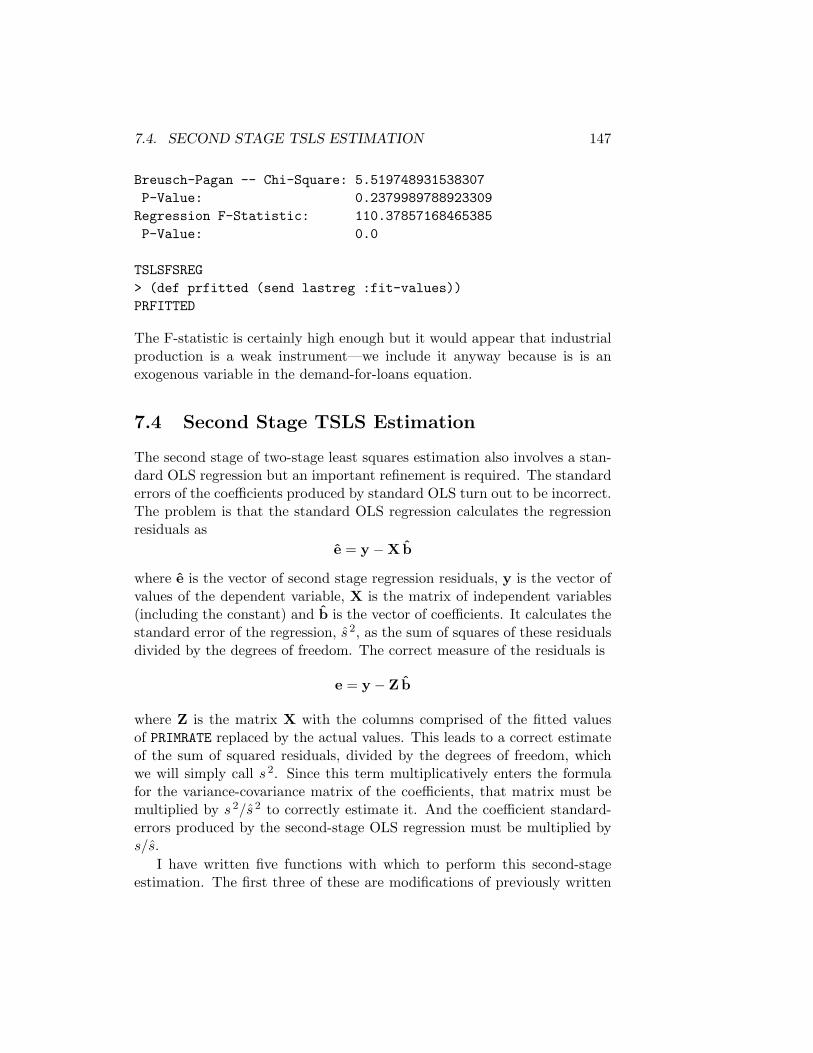
7.4. SECOND STAGE TSLS ESTIMATION 147
Breusch-Pagan -- Chi-Square: 5.519748931538307P-Value: 0.2379989788923309
Regression F-Statistic: 110.37857168465385P-Value: 0.0
TSLSFSREG> (def prfitted (send lastreg :fit-values))PRFITTED
The F-statistic is certainly high enough but it would appear that industrialproduction is a weak instrument—we include it anyway because is is anexogenous variable in the demand-for-loans equation.
7.4 Second Stage TSLS Estimation
The second stage of two-stage least squares estimation also involves a stan-dard OLS regression but an important refinement is required. The standarderrors of the coefficients produced by standard OLS turn out to be incorrect.The problem is that the standard OLS regression calculates the regressionresiduals as
e = y −Xb
where e is the vector of second stage regression residuals, y is the vector ofvalues of the dependent variable, X is the matrix of independent variables(including the constant) and b is the vector of coefficients. It calculates thestandard error of the regression, s 2, as the sum of squares of these residualsdivided by the degrees of freedom. The correct measure of the residuals is
e = y − Z b
where Z is the matrix X with the columns comprised of the fitted valuesof PRIMRATE replaced by the actual values. This leads to a correct estimateof the sum of squared residuals, divided by the degrees of freedom, whichwe will simply call s 2. Since this term multiplicatively enters the formulafor the variance-covariance matrix of the coefficients, that matrix must bemultiplied by s 2/s 2 to correctly estimate it. And the coefficient standard-errors produced by the second-stage OLS regression must be multiplied bys/s.
I have written five functions with which to perform this second-stageestimation. The first three of these are modifications of previously written
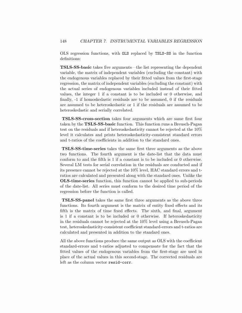
148 CHAPTER 7. INSTRUMENTAL VARIABLES REGRESSION
OLS regression functions, with OLS replaced by TSLS-SS in the functiondefinitions:
TSLS-SS-basic takes five arguments—the list representing the dependentvariable, the matrix of independent variables (excluding the constant) withthe endogenous variables replaced by their fitted values from the first-stageregression, the matrix of independent variables (excluding the constant) withthe actual series of endogenous variables included instead of their fittedvalues, the integer 1 if a constant is to be included or 0 otherwise, andfinally, -1 if homoskedastic residuals are to be assumed, 0 if the residualsare assumed to be heteroskedastic or 1 if the residuals are assumed to beheteroskedastic and serially correlated.
TSLS-SS-cross-section takes four arguments which are same first fourtaken by the TSLS-SS-basic function. This function runs a Breusch-Pagantest on the residuals and if heteroskedasticity cannot be rejected at the 10%level it calculates and prints heteroskedasticity-consistent standard errorsand t-ratios of the coefficients in addition to the standard ones.
TSLS-SS-time-series takes the same first three arguments as the abovetwo functions. The fourth argument is the date-list that the data mustconform to and the fifth is 1 if a constant is to be included or 0 otherwise.Several LM tests for serial correlation in the residuals are conducted and ifits presence cannot be rejected at the 10% level, HAC standard errors and t-ratios are calculated and presented along with the standard ones. Unlike theOLS-time-series function, this function cannot be applied to sub-periodsof the date-list. All series must conform to the desired time period of theregression before the function is called.
TSLS-SS-panel takes the same first three arguments as the above threefunctions. Its fourth argument is the matrix of entity fixed effects and itsfifth is the matrix of time fixed effects. The sixth, and final, argumentis 1 if a constant is to be included or 0 otherwise. If heteroskedasticityin the residuals cannot be rejected at the 10% level using a Breusch-Pagantest, heteroskedasticity-consistent coefficient standard-errors and t-ratios arecalculated and presented in addition to the standard ones.
All the above functions produce the same output as OLS with the coefficientstandard-errors and t-ratios adjusted to compensate for the fact that thefitted values of the endogenous variables from the first-stage are used inplace of the actual values in this second-stage. The corrected residuals areleft as the column vector resid-corr.
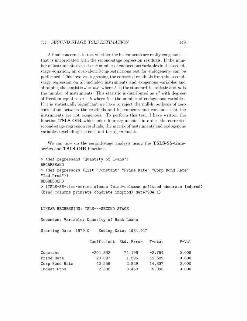
7.4. SECOND STAGE TSLS ESTIMATION 149
A final concern is to test whether the instruments are really exogenous—that is uncorrelated with the second-stage regression residuals. If the num-ber of instruments exceeds the number of endogenous variables in the second-stage equation, an over-identifying-restrictions test for endogeneity can beperformed. This involves regressing the corrected residuals from the second-stage regression on all included instruments and exogenous variables andobtaining the statistic J = mF where F is the standard F-statistic and m isthe number of instruments. This statistic is distributed as χ2 with degreesof freedom equal to m − k where k is the number of endogenous variables.If it is statistically significant we have to reject the null-hypothesis of zerocorrelation between the residuals and instruments and conclude that theinstruments are not exogenous. To perform this test, I have written thefunction TSLS-OIR which takes four arguments—in order, the correctedsecond-stage regression residuals, the matrix of instruments and exdogenousvariables (excluding the constant term), m and k.
We can now do the second-stage analysis using the TSLS-SS-time-series and TSLS-OIR functions.
> (def regressand "Quantity of Loans")REGRESSAND> (def regressors (list "Constant" "Prime Rate" "Corp Bond Rate""Ind Prod"))REGRESSORS> (TSLS-SS-time-series qloans (bind-columns prfitted cbndrate indprod)(bind-columns primrate cbndrate indprod) date7984 1)
LINEAR REGRESSION: TSLS---SECOND STAGE
Dependent Variable: Quantity of Bank Loans
Starting Date: 1979.0 Ending Date: 1984.917
Coefficient Std. Error T-stat P-Val
Constant -204.332 74.196 -2.754 0.008Prime Rate -20.097 1.596 -12.589 0.000Corp Bond Rate 40.556 2.829 14.337 0.000Indust Prod 2.306 0.453 5.095 0.000

150 CHAPTER 7. INSTRUMENTAL VARIABLES REGRESSION
Number of Observations: 72Degrees of Freedom: 68R-Squared: 0.9061881342923508Adjusted R-Squared: 0.902049375511131Sum of Squared Errors: 24359.11492524487Regression F-Statistic: 218.9516669597422P-Value: 0.0
LM-Based Test for Serial Correlation in Residuals:Order = 1 Chisq-stat = 99.49112458999178 P-Value = 0.0
LM-Based Test for Serial Correlation in Residuals:Order =< 3 Chisq-stat = 112.22572656626016 P-Value = 0.0
LM-Based Test for Serial Correlation in Residuals:Order =< 18 Chisq-stat = 105.37237073901618 P-Value =2.275957200481571E-14
Modified Results Using HAC Standard Errors of Coefficients:Truncation lag = 3
Coefficient Std. Error T-stat P-Val
Constant -204.332 124.899 -1.636 0.106Prime Rate -20.097 2.148 -9.358 0.000Corp Bond Rate 40.556 4.142 9.792 0.000Indust Prod 2.306 0.695 3.317 0.001
NIL> (TSLS-OIR (copy-matrix-column 0 resids-corr)(bind-columns cbndrateindprod tbrate totbdep) 2 1)
Test of Over-identifying RestrictionsJ = 14.544083005422333P-Value = 1.3691796589743177E-4
NIL
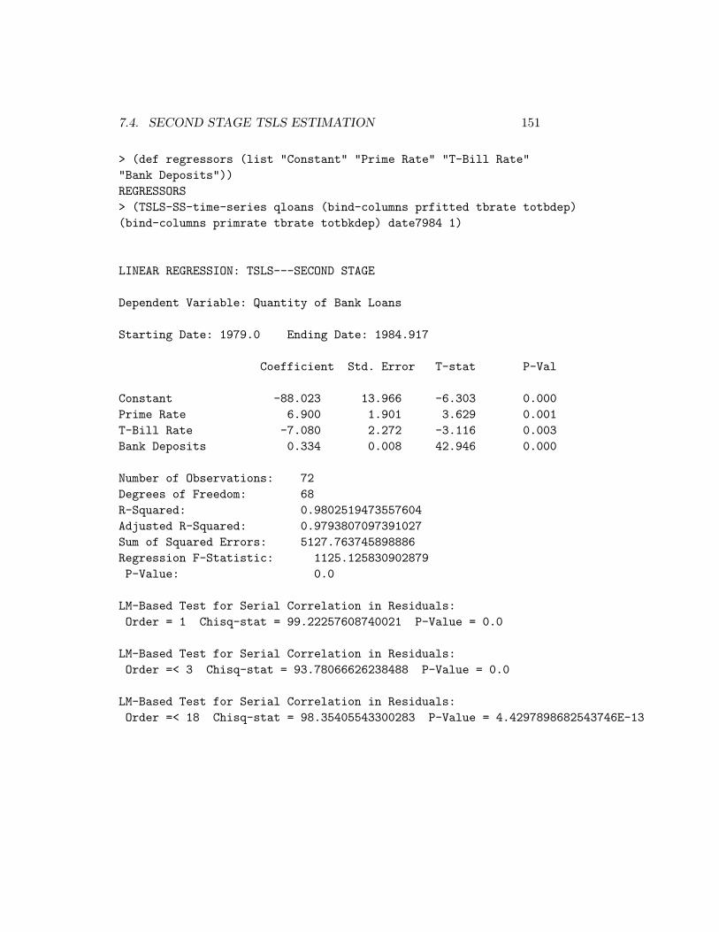
7.4. SECOND STAGE TSLS ESTIMATION 151
> (def regressors (list "Constant" "Prime Rate" "T-Bill Rate""Bank Deposits"))REGRESSORS> (TSLS-SS-time-series qloans (bind-columns prfitted tbrate totbdep)(bind-columns primrate tbrate totbkdep) date7984 1)
LINEAR REGRESSION: TSLS---SECOND STAGE
Dependent Variable: Quantity of Bank Loans
Starting Date: 1979.0 Ending Date: 1984.917
Coefficient Std. Error T-stat P-Val
Constant -88.023 13.966 -6.303 0.000Prime Rate 6.900 1.901 3.629 0.001T-Bill Rate -7.080 2.272 -3.116 0.003Bank Deposits 0.334 0.008 42.946 0.000
Number of Observations: 72Degrees of Freedom: 68R-Squared: 0.9802519473557604Adjusted R-Squared: 0.9793807097391027Sum of Squared Errors: 5127.763745898886Regression F-Statistic: 1125.125830902879P-Value: 0.0
LM-Based Test for Serial Correlation in Residuals:Order = 1 Chisq-stat = 99.22257608740021 P-Value = 0.0
LM-Based Test for Serial Correlation in Residuals:Order =< 3 Chisq-stat = 93.78066626238488 P-Value = 0.0
LM-Based Test for Serial Correlation in Residuals:Order =< 18 Chisq-stat = 98.35405543300283 P-Value = 4.4297898682543746E-13

152 CHAPTER 7. INSTRUMENTAL VARIABLES REGRESSION
Modified Results Using HAC Standard Errors of Coefficients:Truncation lag = 3
Coefficient Std. Error T-stat P-Val
Constant -88.023 19.403 -4.537 0.000Prime Rate 6.900 2.532 2.725 0.008T-Bill Rate -7.080 3.060 -2.314 0.024Bank Deposits 0.334 0.014 24.279 0.000
NIL
> (TSLS-OIR (copy-matrix-column 0 resids-corr)(bind-columns cbndrateindprod tbrate totbdep) 2 1)
Test of Over-identifying RestrictionsJ = 2.2886547103520276P-Value = 0.13032283784027232
We have to conclude that one or both instruments are not exogenous in theestimation of the demand function for loans, although both appear to beexogenous in the estimation of the supply function.
7.5 An Application to Panel Data
Another interesting instrumental variables problem is presented by Stockand Watson in Chapter 10 of the textbook referred to earlier. They examinea annual panel data set dealing with cigarette consumption and the factorsaffecting it in 48 U.S. states during the years 1985 and 1995. The objectis to determine whether an increase in the price of cigarettes will reducecigarette consumption by an economically significant amount—that is, tomeasure the elasticity of demand for cigarettes. The dataset, which hasbeen copied to the file cigdata.lsp contains the following variables.
PACKPC —Packages of Cigarettes Consumed Per CapitaAVGPRS —Average Price of a Package of CigarettesTAX —Taxes on CigarettesTAXS —General Sales TaxCPI —U.S. Consumer Price IndexINCOME —IncomePOP —PopulationENTITY —Entity Code – (1, 2, 3, .... 48)YEAR —Year – (1985, 1995)
All prices and general sales taxes are measured in cents per package.

7.5. AN APPLICATION TO PANEL DATA 153
> (load "addfuncs"); loading addfuncs.lspT> (load "cigdata"); loading cigdata.lspT> (variables)(AVGPRS CPI ENTITY INCOME PACKPC POP TAX TAXS YEAR)
Because of variations in the supply curve, the price per package will almostsurely be correlated with the error term in an OLS estimate of the demandcurve. Useful instruments appear to be the cigarette tax and sales taxvariables since they should both be positively correlated with the price perpackage and should be exogenous with respect to the error term in the OLSestimated demand curve.
Our first step, after converting income into per-capita terms, expressingall prices in real terms (deflating by the CPI) and taking logarithms, is toconvert the data into 1995-1985 differences as a way of eliminating entityfixed effects.
> (def income (/ income pop))INCOME> (def income (log (/ income cpi)))INCOME> (def avgprs (log (/ avgprs cpi)))AVGPRS> (def tax (log (/ tax cpi)))TAX> (def taxs (log (/ taxs cpi)))TAXS> (def packpc (log packpc))PACKPC> (def obslist-85 (panel-collect-obsnums year entity 1985))OBSLIST-85> (def obslist-95 (panel-collect-obsnums year entity 1995))OBSLIST-95> (def packpc-85 (select packpc obslist-85))PACKPC-85> (def packpc-95 (select packpc obslist-95))PACKPC-95> (def income-85 (select income obslist-85))INCOME-85

154 CHAPTER 7. INSTRUMENTAL VARIABLES REGRESSION
> (def income-95 (select income obslist-95))INCOME-95> (def tax-85 (select tax obslist-85))TAX-85> (def tax-95 (select tax obslist-95))TAX-95> (def taxs-85 (select taxs obslist-85))TAXS-85> (def taxs-95 (select taxs obslist-95))TAXS-95> (def avgprs-85 (select avgprs obslist-85))AVGPRS-85> (def avgprs-95 (select avgprs obslist-95))AVGPRS-95> (def quant-dif (- packpc-95 packpc-85))QUANT-DIF> (def income-dif (- income-95 income-85))INCOME-DIF> (def price-dif (- avgprs-95 avgprs-85))PRICE-DIF> (def cigtax-dif (- tax-95 tax-85))CIGTAX-DIF> (def salestax-dif (- taxs-95 taxs-85))SALESTAX-DIF
Next, we can estimate the demand curve by OLS to see what the biasedcoefficients will be.
> (def regressand "quant-dif")REGRESSAND> (def regressors (list "Constant" "price-dif" "income-dif"))REGRESSORS> (def reg0 (OLS-basic quant-dif (bind-columns price-difincome-dif) 1 -1))

7.5. AN APPLICATION TO PANEL DATA 155
LINEAR REGRESSION
Dependent Variable: quant-dif
Coefficient Std. Error T-stat P-Val
Constant -0.085 0.059 -1.453 0.153price-dif -1.056 0.149 -7.081 0.000income-dif 0.498 0.304 1.636 0.109
Number of Observations: 48Degrees of Freedom: 45R-Squared: 0.5559789872632931Adjusted R-Squared: 0.5362447200305506Sum of Squared Errors: 0.3669425174766015LMSC -- Chi-Square: 1.6365558452394362P-Value: 0.20079867559105202
Breusch-Pagan -- Chi-Square: 0.7546624898846197P-Value: 0.6856889052919959
Regression F-Statistic: 28.173277512976448P-Value: 1.1656797971326682E-8
REG0
Now we can run the first stage of our two-stage least squares analysis usingthe OLS-basic function with the cigarette and general sales taxes as in-struments and per capita income included as the exogenous regressor. TheF-statistic in excess of 24 indicates that the instruments are relevant.
> (def regressand "price-dif")REGRESSAND> (def regressors (list "Constant" "cigtax-dif" "salestax-dif""income-dif"))REGRESSORS> (def regfs (OLS-basic price-dif (bind-columns cigtax-difsalestax-dif income-dif) 1 -1))
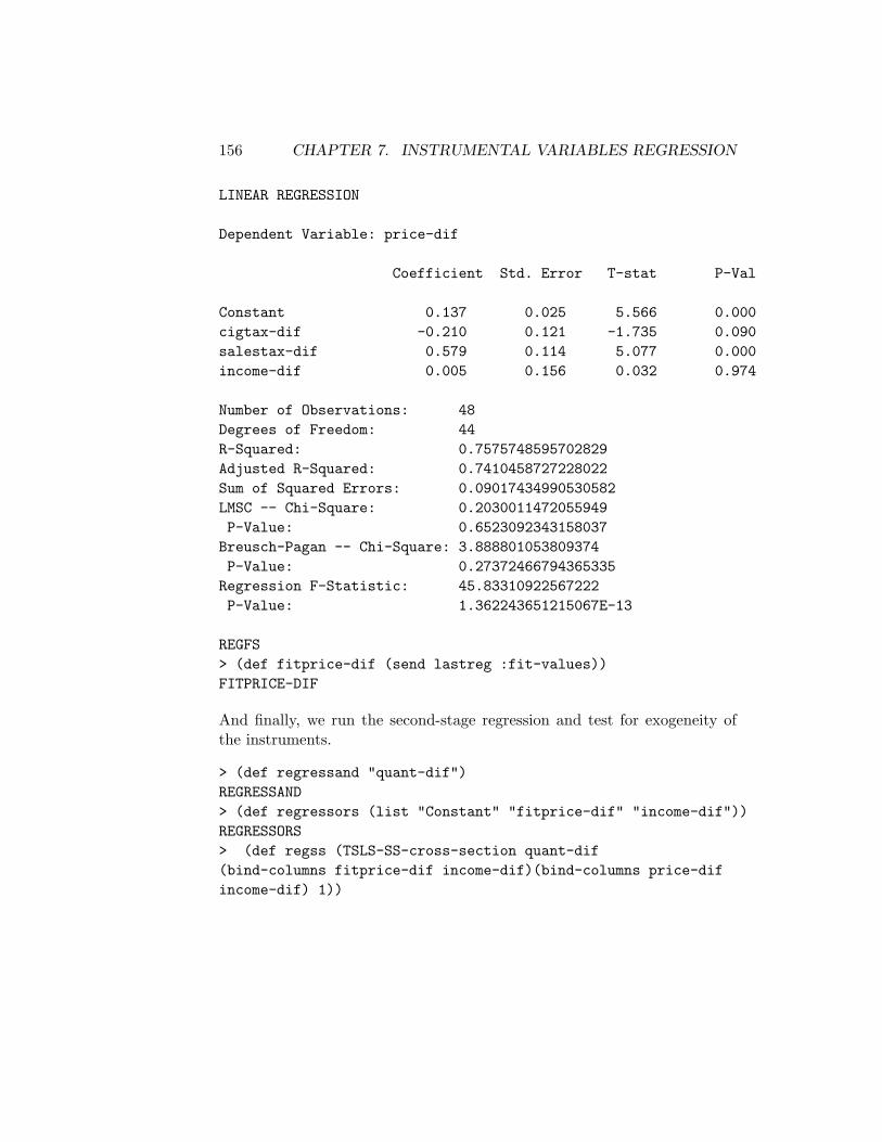
156 CHAPTER 7. INSTRUMENTAL VARIABLES REGRESSION
LINEAR REGRESSION
Dependent Variable: price-dif
Coefficient Std. Error T-stat P-Val
Constant 0.137 0.025 5.566 0.000cigtax-dif -0.210 0.121 -1.735 0.090salestax-dif 0.579 0.114 5.077 0.000income-dif 0.005 0.156 0.032 0.974
Number of Observations: 48Degrees of Freedom: 44R-Squared: 0.7575748595702829Adjusted R-Squared: 0.7410458727228022Sum of Squared Errors: 0.09017434990530582LMSC -- Chi-Square: 0.2030011472055949P-Value: 0.6523092343158037Breusch-Pagan -- Chi-Square: 3.888801053809374P-Value: 0.27372466794365335Regression F-Statistic: 45.83310922567222P-Value: 1.362243651215067E-13
REGFS> (def fitprice-dif (send lastreg :fit-values))FITPRICE-DIF
And finally, we run the second-stage regression and test for exogeneity ofthe instruments.
> (def regressand "quant-dif")REGRESSAND> (def regressors (list "Constant" "fitprice-dif" "income-dif"))REGRESSORS> (def regss (TSLS-SS-cross-section quant-dif(bind-columns fitprice-dif income-dif)(bind-columns price-difincome-dif) 1))

7.5. AN APPLICATION TO PANEL DATA 157
LINEAR REGRESSION: TSLS--SECOND STAGE
Dependent Variable: quant-dif
Coefficient Std. Error T-stat P-Val
Constant -0.048 0.063 -0.759 0.452fitprice-dif -1.200 0.173 -6.918 0.000income-dif 0.463 0.308 1.502 0.140
Number of Observations: 48Degrees of Freedom: 45R-Squared: 0.5433378444067236Adjusted R-Squared: 0.523041748602578Sum of Squared Errors: 0.377389259073314
Breusch-Pagan test on the ResidualsChi-Square Statistic = 0.9141069794299526P-Value = 0.633146472332637
REGSS> (TSLS-OIR (copy-matrix-column 0 resids-corr)(bind-columns cigtax-dif salestax-dif income-dif) 2 1)
Test of Over-identifying RestrictionsJ = 5.372354636942074P-Value = 0.020458342334803037
NIL
The demand elasticity has the correct sign and is somewhat larger thanwhen the function was estimated by ordinary OLS. The over-identifying-restrictions test indicates that at least one of the two instruments is notexogenous. It turns out that when Stock and Watson redo the calculationsusing each instrument alone in turn they obtain correctly signed demandelasticities that bracket the one above. Unfortunately, with only one instru-ment there is no way of testing it for exogeneity.3
3The coefficient standard-errors differ here from those reported by Stock and Watsonbecause our TSLS-SS-cross-section function did not use HAC coefficient standard er-rors, given that the Breusch-Pagan test indicates no statistically significant heteroskedas-

158 CHAPTER 7. INSTRUMENTAL VARIABLES REGRESSION
It is interesting to note that both our two-stage least squares estimatesof demand functions in this chapter suffered from evident lack of instrumentexogeneity. In view of the fact that the standard OLS estimates of thedemand functions yielded correctly signed elasticities, do we gain anythingby basing our conclusions on the instrumental variables estimates instead?
ticity in the second-stage regression residuals. Stock and Watson routinely report onlyHAC coefficient standard-errors. They also routinely report HAC regression F-statisticswhereas all functions thus-far used in this work produce only the standard ones. Whilethe constants differ in magnitude between our results and those of Stock and Watson, thisfact is of little consequence as the difference most likely depends on a different scaling ofthe variables.

Chapter 8
Probit, Logit and NonlinearRegression
Another set of issues arise when the dependent variable is binary—that is,takes a value of zero or unity. An example is the problem of determiningwhether, other things equal, blacks are more often denied residential mort-gages than whites in the Boston area. A data set for analysing this problem,which forms the basis for the analysis of Stock and Watson in Chapter 9of their introductory econometrics textbook, was obtained and refined inChapter 2 of this manual. The Stock and Watson Chapter is an excellentreference for those needing to upgrade their understanding of the basics.The dependent variable is the variable DENY, which takes a value of 1 if theindividual is denied a mortgage and 0 otherwise. Here, we are interested inonly two independent variables, the ratio of total monthly debt obligationsto income, denoted by RTDINC and the variable BLACK, which takes a valueof 1 if the applicant is black and 0 if the applicant is white. Readers can usethe remaining data for refining the results presented here.
8.1 The Linear Probability Model
One way of analysing this issue is simply to regress DENY on the two variablesRTDINC and BLACK, together with a constant term. Using our OLS-Basicfunction, we proceed as follows, ending with a plot of the fitted values againstthe ratio of total payments to income.
> (load "addfuncs.lsp"); loading addfuncs.lsp
159

160 CHAPTER 8. PROBIT, LOGIT AND NONLINEAR REGRESSION
T
> (load "hmdata"); loading hmdata.lspT> (variables)(AMT BLACK CCSCORE CONDO DENMINS DENY HSGRAD MCSCORE OBS-ADJPROPVAL PUBREC RHDINC RTDINC SELFEMP SINGLE UNRATE)> (def regressand "Probability of Denial")REGRESSAND> (def regressors (list "Constant" "Payments/Income" "Black"))REGRESSORS> (def reg0 (OLS-basic deny (bind-columns rtdinc black) 1 -1))
LINEAR REGRESSION
Dependent Variable: Probability of Denial
Coefficient Std. Error T-stat P-Val
Constant -0.121 0.027 -4.504 0.000Payments/Income 0.653 0.080 8.201 0.000Black 0.176 0.019 9.522 0.000
Number of Observations: 2351Degrees of Freedom: 2348R-Squared: 0.0704528991455754Adjusted R-Squared: 0.06966112137653424Sum of Squared Errors: 229.27510542044902LMSC -- Chi-Square: 148.12782736404145P-Value: 0.0Breusch-Pagan -- Chi-Square: 102.49402936375255P-Value: 0.0Regression F-Statistic: 88.98064823275585P-Value: 0.0
REG0
8.2. PROBIT AND LOGIT MODELS 161
> (def fitt0 (send lastreg :fit-values))FITTED> (def plt0 (plot-points rtdinc deny))PLT0NIL> (send plt0 :add-points rtdinc fitt0)NIL> (send plt0 :variable-label 0 "All Payments / Income")NIL> (send plt0 :variable-label 1 "Probability of Denial")NIL
The fitted values, which give the probability of denial at each ratio of totaldebt payments to income appear along the two upward-sloping lines in theplot in Figure 13. The lower line gives the fitted values for individuals whoare white and the upper line gives the fitted values for blacks. The P-Valueof the coefficient of BLACK in the regression print-out above indicates clearlythat the variable is positive and statistically significant—the plot gives avisual indication of the magnitude. The probability that a black home buyerwill be denied a mortgage will always be higher than the probability thata white buyer will be denied at every given level of the ratio of total debtpayments to income.
The problem is that when the ratio of total debt payments to income isless than 0.2, the fitted values are negative—an impossible situation sincethe probability of an occurrence can never be negative. The reason is thatthe true relationship between the probability of denial and the payments-to-income ratio is non-linear and our linear probability model is making alinear approximation to that non-linear relationship.
8.2 Probit and Logit Models
It obviously makes sense to use models in which the probability of the de-pendent variable taking a value of unity ranges between 0 and 1. Probitand logit models are based on cumulative distribution functions, which havethis characteristic. The probit regression model uses the standard normalc.d.f. and the logit regression model uses the logistic c.d.f. The probit re-gression model can be written as
Pr(Y = 1|X1, X2) = Pr(Z) = Φsn(Z)

162 CHAPTER 8. PROBIT, LOGIT AND NONLINEAR REGRESSION
Figure 13: Plot of probability of denial (fitted) against the ratioof total payments to income. The horizontal lines arethe actual levels of DENY and RTDINC.
where Φsn(Z) gives the standard normal cumulative probability at the quan-tile Z with
Z = β0 + β1X1 + β2X2
where X1 and X2 are the independent variables, RTDINC and BLACK, in theexample above, with Y being the variable DENY.
The logit regression model differs from the probit model above in thatΦsn(Z) is replaced by Φlo(Z), the logistic cumulative probability of Z, whichequals
Φlo(Z) =1
e−Z=
1e−(β0+β1X1+β2X2)
.

8.3. NONLINEAR LEAST SQUARES ESTIMATION 163
8.3 Nonlinear Least Squares Estimation
Probit estimation by nonlinear least squares involves choosing the values ofthe β coefficients above that will minimise
Yt − Φsn(β0 + β1X1 + β2X2)
The first step is to set up the function that is to be fitted to the data.Operating in batch mode, our function is
(def idepvars (list rtdinc black))(defun nllsfunc (beta)(def sumterm (select beta 0))(dotimes (i (length idepvars))(def sumterm (+ sumterm (* (select beta (+ i 1))(select idepvars i))))) ; end dotimes(normal-cdf sumterm)) ; end of function
The first line says that the function arguments consist of the list beta, whichis assigned a length and values in subsequent code-lines. Line two sets upthe constant term as the beginning of a sum of terms. The dotimes functionthen loops through the elements of the list idepvars, which contains theindependent variables other than the constant term, multiplying each listby the relevant element of the list beta. The line (normal-cdf sumterm)takes the cumulative normal density of the resulting sum. We then set up alist of initial guesses as to the elements in the coefficient-list beta. A usefulguess is that the constant is zero and the coefficients of the other variablesequal their means.
(def initvals (list 0 (mean rtdinc)(mean black)))
Then, after making sure that the function file maximize.lsp is in theworkspace, we can use the nreg-model function provided in XLispStat asfollows.
(load "maximize")(def nllsreg (nreg-model #’nllsfunc deny initvals))Residual sum of squares: 677.032Residual sum of squares: 236.694Residual sum of squares: 225.974Residual sum of squares: 225.014Residual sum of squares: 224.926Residual sum of squares: 224.918Residual sum of squares: 224.917

164 CHAPTER 8. PROBIT, LOGIT AND NONLINEAR REGRESSION
Least Squares Estimates:
Parameter 0 -2.95899 (0.166013)Parameter 1 4.66769 (0.414271)Parameter 2 0.699485 (6.828708E-2)
R Squared: 8.812298E-2Sigma hat: 0.309501Number of cases: 2351Degrees of freedom: 2348
The resulting object, to which we have assigned the name nllsreg, canbe sent messages to retrieve all of the variables that can be retrieved fromthe regression-model function plus a few more. We can find out exactlywhat these are by inserting our favourite profanity (which XLispStat, beingof high moral tone, will not recognise) causing the execution to stop withan error message. Then we can enter a help message to obtain the list ofmessages our nllsreg object will respond to.
Error: The variable SHIT is unbound.> (send nllsreg :help)NREG-MODEL-PROTONormal Linear Regression ModelHelp is available on the following:
ADD-METHOD ADD-SLOT BASIS CASE-LABELS COEF-ESTIMATESCOEF-STANDARD-ERRORS COMPUTE COOKS-DISTANCES COUNT-LIMITDELETE-DOCUMENTATION DELETE-METHOD DELETE-SLOT DF DISPLAYDOC-TOPICS DOCUMENTATION EPSILON EXTERNALLY-STUDENTIZED-RESIDUALSFIT-VALUES GET-METHOD HAS-METHOD HAS-SLOT HELP INCLUDED INTERCEPTINTERNAL-DOC ISNEW LEVERAGES MEAN-FUNCTION METHOD-SELECTORSNEW NEW-INITIAL-GUESS NUM-CASES NUM-COEFS NUM-INCLUDEDOWN-METHODS OWN-SLOTS PARAMETER-NAMES PARENTS PLOT-BAYES-RESIDUALSPLOT-RESIDUALS PRECEDENCE-LIST PREDICTOR-NAMES PRINT PROTOR-SQUARED RAW-RESIDUALS REPARENT RESIDUAL-SUM-OF-SQUARESRESIDUALS RESPONSE-NAME RETYPE SAVE SHOW SIGMA-HAT SLOT-NAMESSLOT-VALUE STUDENTIZED-RESIDUALS SUM-OF-SQUARES SWEEP-MATRIXTHETA-HAT TOTAL-SUM-OF-SQUARES VERBOSE WEIGHTS X X-MATRIXXTXINV YNIL

8.3. NONLINEAR LEAST SQUARES ESTIMATION 165
For a clearer presentation of the results, I have written the function NLLSwhich takes three arguments in the following order—the name of the de-pendent variable list, a list containing the independent variables lists ex-cluding the constant, and a list of initial guesses as to the coefficients of allvariables including the constant. An appropriate function called nllsfuncmust previously have been written and be present in the workspace. And, aswith all the other regression functions, a string-object called regressand,giving the name assigned to the dependent variable, and a list of stringscalled regressors, giving the names of the independent variables includingthe constant term, must be present in the work-space when the function iscalled. A regression-model object called nllsreg is left in the workspacealong with the variables coefs, stderrs, tratios, df, nobs, SSE, TSS andMSE. Using the NLLS function in the above case, we obtain the followingresults.
> (def reg1 (NLLS deny idepvars initvals))
MINIMIZING THE SUM OF SQUARES IN NON-LINEAR REGRESSION
REGRESSION RESULTS
Dependent Variable: Probability of Denial
Coefficient Std. Error T-stat P-Val
Constant -2.959 0.166 -17.824 0.000All Payts/Inc 4.668 0.414 11.267 0.000Black 0.699 0.068 10.243 0.000
Number of Observations: 2351Degrees of Freedom: 2348Standard Error 0.09579077311734745R-Squared: 0.08812298295825427
REG1
We can then extract the fitted values from the object reg1 and plot thesein the form that appears in Figure 14.
> (def fitt1 (send reg1 :fit-values))FITT1
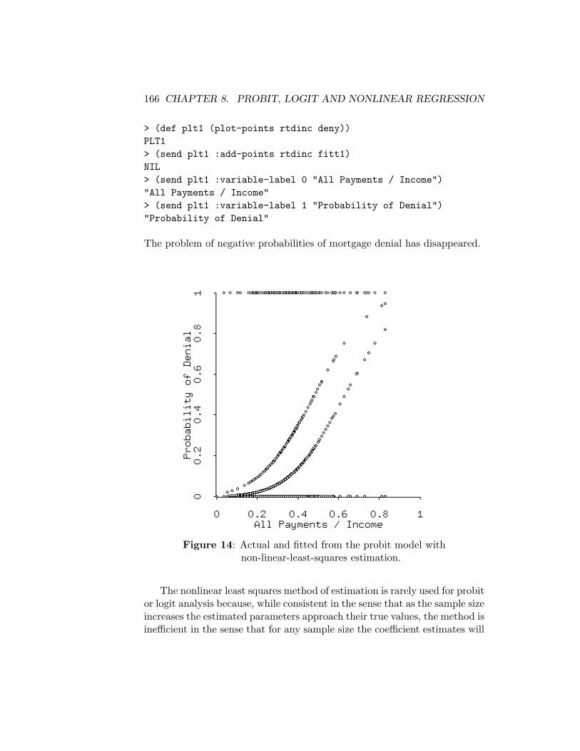
166 CHAPTER 8. PROBIT, LOGIT AND NONLINEAR REGRESSION
> (def plt1 (plot-points rtdinc deny))PLT1> (send plt1 :add-points rtdinc fitt1)NIL> (send plt1 :variable-label 0 "All Payments / Income")"All Payments / Income"> (send plt1 :variable-label 1 "Probability of Denial")"Probability of Denial"
The problem of negative probabilities of mortgage denial has disappeared.
Figure 14: Actual and fitted from the probit model withnon-linear-least-squares estimation.
The nonlinear least squares method of estimation is rarely used for probitor logit analysis because, while consistent in the sense that as the sample sizeincreases the estimated parameters approach their true values, the method isinefficient in the sense that for any sample size the coefficient estimates will

8.4. MAXIMUM LIKELIHOOD ESTIMATION 167
have a larger variance than when an alternative, the method of maximumlikelihood estimation is used.
My purpose in using nonlinear least squares here was simply to demon-strate how the method works so that the reader can apply it, where appro-priate, to other situations where the function being estimated is nonlinear.All that is required is to modify appropriately the nllsfunc to correctlyrepresent the function being estimated and, with that object present in theworkspace, construct an appropriate list of initial values and call the NLLSfunction.
8.4 Maximum Likelihood Estimation
Maximum likelihood estimation involves choosing the β coefficients so asto maximize the logarithm of the likelihood function, which for the probitmodel is
L =n∑
i=1
Yi ln(Φsn) +n∑
i=1
(1− Yi) ln(1− Φsn)
and, for the logit model
L =n∑
i=1
Yi ln(Φlo) +n∑
i=1
(1− Yi) ln(1− Φlo)
where Φsn and Φlo are defined in exactly the same way as in the case ofnonlinear least squares estimation.1
We begin by writing appropriate code for the function to be maximized,probfunc, which will appear in batch file mode as follows.
(def const (repeat 1 (length deny)))(def variables (list const rtdinc black));(defun probfunc (theta)(def z 0)(dotimes (i (length variables))(setf z (+ z (* (select variables i)(select theta i))))) ; end dotimes i
1A discussion of how the likelihood function is derived can be found on page 326 of theStock and Watson book.
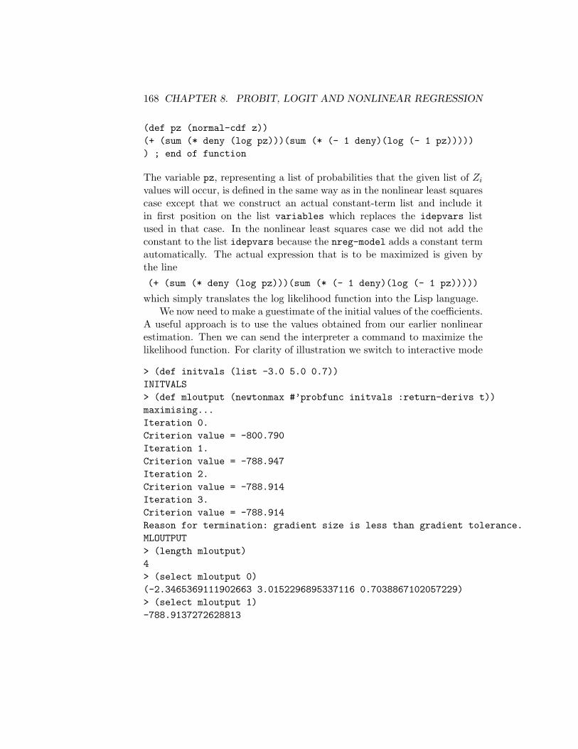
168 CHAPTER 8. PROBIT, LOGIT AND NONLINEAR REGRESSION
(def pz (normal-cdf z))(+ (sum (* deny (log pz)))(sum (* (- 1 deny)(log (- 1 pz)))))) ; end of function
The variable pz, representing a list of probabilities that the given list of Zi
values will occur, is defined in the same way as in the nonlinear least squarescase except that we construct an actual constant-term list and include itin first position on the list variables which replaces the idepvars listused in that case. In the nonlinear least squares case we did not add theconstant to the list idepvars because the nreg-model adds a constant termautomatically. The actual expression that is to be maximized is given bythe line(+ (sum (* deny (log pz)))(sum (* (- 1 deny)(log (- 1 pz)))))
which simply translates the log likelihood function into the Lisp language.We now need to make a guestimate of the initial values of the coefficients.
A useful approach is to use the values obtained from our earlier nonlinearestimation. Then we can send the interpreter a command to maximize thelikelihood function. For clarity of illustration we switch to interactive mode
> (def initvals (list -3.0 5.0 0.7))INITVALS> (def mloutput (newtonmax #’probfunc initvals :return-derivs t))maximising...Iteration 0.Criterion value = -800.790Iteration 1.Criterion value = -788.947Iteration 2.Criterion value = -788.914Iteration 3.Criterion value = -788.914Reason for termination: gradient size is less than gradient tolerance.MLOUTPUT> (length mloutput)4> (select mloutput 0)(-2.3465369111902663 3.0152296895337116 0.7038867102057229)> (select mloutput 1)-788.9137272628813
8.4. MAXIMUM LIKELIHOOD ESTIMATION 169
> (select mloutput 2)(-5.600921040393025E-7 -1.4739872449923207E-7 -1.0818945488287528E-8)> (print-matrix (select mloutput 3))#2a(
( -816.345 -282.119 -184.784 )( -282.119 -103.456 -66.0983 )( -184.784 -66.0983 -184.784 )
)NIL
The newtonmax function maximizes the log likelihood function using New-ton’s method. Its output, which we have defined as the object mloutputconsists of a list. The first element is the list of coefficients, the secondis the maximized value of the log-likelihood, the third is the gradient, andthe fourth is the hessian matrix. The standard-errors of the coefficients canbe found by multiplying the hessian matrix by -1, taking the inverse, andthen extracting the square roots of the resulting diagonal elements. If thenewtonmax function cannot find a maximum, we can use the Nelder-Meadsimplex method via the nelmeadmax function by entering the following com-mand line.
> (def mloutput (nelmeadmax #’probfunc initvals :return-derivs t))Value = -800.7899312386357Value = -800.7899312386357Value = -800.7899312386357Value = -800.7899312386357Value = -800.7899312386357
..............
..............
..............
Value = -788.9137274028564Value = -788.9137274028564Value = -788.9137274028564Value = -788.9137273503475MLOUTPUT
Unfortunately, the output returned by this function consists only of the threecoefficients, leaving no prospect of calculating their standard-errors. Thetrick, then, is to use this function to obtain the coefficient values when thenewtonmax function fails to find a maximum and then feed these coefficient-

170 CHAPTER 8. PROBIT, LOGIT AND NONLINEAR REGRESSION
values as initial guesses to the newtonmax function. To obtain a full pre-sentation, I have constructed a function called probit which takes as itsarguments in the following order, the dependent variable list, a string objectgiving the name of the dependent variable, the list of independent variablescalled variables which should be in the workspace when the function iscalled, a list of strings called varnames comprising the names of all indepen-dent variables including the constant, and a list giving the initial guesses asto the magnitudes of the parameters. This function, which also calculatesthe log likelihood to be maximized, yields the following result.
> (probit deny "Probability of Denial" variables varnamesinitvals)
DETAILS OF PROBIT LOG LIKELIHOOD MAXIMIZATIONmaximizing...Iteration 0.Criterion value = -800.790Iteration 1.Criterion value = -788.947Iteration 2.Criterion value = -788.914Iteration 3.Criterion value = -788.914Reason for termination: gradient size is less than gradient tolerance.
PROBIT REGRESSION RESULTS
Dependent Variable: Probability of Denial
Coefficient Std. Error T-stat P-Val Elasticity
Constant -2.347 0.146 -16.066 0.004All Payts/Inc 3.015 0.411 7.339 0.004 1.734Black 0.704 0.084 8.391 0.018 0.170
Log Likelihood with all variables included = -788.9137272628813Log Likelihood with constant term only = -858.4076312800587The Pseudo-R-Square = 0.08095676399515228Likelihood Ratio Statistic for regression = 138.98780803435488
P-Value = 0.0

8.4. MAXIMUM LIKELIHOOD ESTIMATION 171
Number with predicted > .5 that are 1 = 8Total number that are 1 = 280Number with predicted < .5 that are 0 = 2067Total number that are 0 = 2071Number of correct predictions = 2075Total number of cases = 2351Fraction correctly predicted = 0.8826031475967673
NIL> (def plmax1 likemax)PLMAX1
In addition to the coefficient estimates, the function calculates their stan-dard errors and P-Values (in the limit these are normally distributed) andthe elasticities of response of the probability that the dependent variable willbe 1 to a change in the actual values of the independent variables (changein the mean value in the case of binary variables like BLACK) evaluated attheir mean values. The output from the function also includes a pseudo-R-Square, using McFadden’s method of calculation, and a likelihood ratiostatistic to test the null-hypothesis that all the coefficients but the constantterm are zero, together with its P-Value.2
Finally the output supplies us with information about the predictiveaccuracy of the model culminating in an estimate of the fraction correctlypredicted—that is, the fraction of observations of the dependent variablethat were 1 when the probability of them being 1 exceeded 0.5 or 0 whenthe probability of them being 1 fell short of 0.5. After the probit functiondid its thing, the maximum of the log likelihood function was then saved foruse in further tests that will be discussed later.
We can now plot the actual and fitted values. The latter are left in theworkspace as the list fitted by the probit function.
> (def plt2 (plot-points rtdinc deny))PLT2> (send plt2 :add-points rtdinc fitted)NIL> (send plt2 :variable-label 0 "All Payments / Income")"All Payments / Income"> (send plt2 :variable-label 1 "Probability of Denial")"Probability of Denial"
2D. McFadden, “The Measurement of Urban Travel Demand,” Journal of PoliticalEconomy, Vol. 93, 1974, pp. 417-425. The formula for the pseudo-R-Square is R2 =1−L0/Lβ where Lβ is the value of the log likelihood when all variables are included andL0 is the value with the constant term only. The Likelihood Ratio Statistic, which isdistributed as χ2 with degrees of freedom equal to the number of independent variablesexcluding the constant, is LR = 2(Lβ − L0).
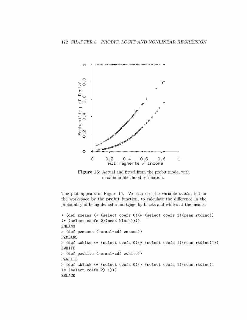
172 CHAPTER 8. PROBIT, LOGIT AND NONLINEAR REGRESSION
Figure 15: Actual and fitted from the probit model withmaximum-likelihood estimation.
The plot appears in Figure 15. We can use the variable coefs, left inthe workspace by the probit function, to calculate the difference in theprobability of being denied a mortgage by blacks and whites at the means.
> (def zmeans (+ (select coefs 0)(* (select coefs 1)(mean rtdinc))(* (select coefs 2)(mean black))))ZMEANS> (def pzmeans (normal-cdf zmeans))PZMEANS> (def zwhite (+ (select coefs 0)(* (select coefs 1)(mean rtdinc))))ZWHITE> (def pzwhite (normal-cdf zwhite))PZWHITE> (def zblack (+ (select coefs 0)(* (select coefs 1)(mean rtdinc))(* (select coefs 2) 1)))ZBLACK
8.4. MAXIMUM LIKELIHOOD ESTIMATION 173
> (def pzblack (normal-cdf zblack))PZBLACK> pzmeans0.10449309629778049> pzwhite0.08735003022819859> pzblack0.2567592964344873
At the means of the independent variables the mean probability of beingdenied mortgage finance is slightly above .1. At the mean value of the ratioof total payments obligations to income, which is about .33, the probabilityof a white person being denied is nearly .09 while the probability of a blackperson being denied is over .25. This represents the vertical distance betweenthe two lines in Figure 15 at the .33 position along the horizontal axis.
Estimation of the logit regression is essentially the same. All that differsis the likelihood function we ask the newtonmax function to maximize. Thecode for this function is as follows.
(defun logitcalc (theta)(def z 0)(dotimes (i (length variables))(setf z (+ z (* (select variables i)(select theta i))))) ; end dotimes i(def pz (/ 1 (+ 1 (exp (* -1 z)))))(+ (sum (* deny (log pz)))(sum (* (- 1 deny)(log (- 1 pz)))))) ; end of function logitcalc
As in the case of the maximum likelihood estimation of the probit function,this function is automatically created by the logit function I wrote to cal-culate and present the results which follow. This function takes exactly thesame arguments as the probit function.
> (logit deny "Probability of Denial" variables varnames initvals)
DETAILS OF LOGIT LOG LIKELIHOOD MAXIMIZATIONmaximizing...Iteration 0.Criterion value = -895.975Iteration 1.Criterion value = -792.901
174 CHAPTER 8. PROBIT, LOGIT AND NONLINEAR REGRESSION
Iteration 2.Criterion value = -786.632Iteration 3.Criterion value = -786.565Iteration 4.Criterion value = -786.565Reason for termination: gradient size is less than gradient tolerance.
LOGIT REGRESSION RESULTS
Dependent Variable: Probability of Denial
Coefficient Std. Error T-stat P-Val Elasticity
Constant -4.352 0.291 -14.940 0.004All Payts/Inc 6.051 0.794 7.622 0.004 1.806Black 1.262 0.147 8.584 0.017 0.158
Log Likelihood with all variables included = -786.5654230654864Log Likelihood with constant term only = -858.4076312800587The Pseudo-R-Square = 0.08369241558051055Likelihood Ratio Statistic for regression = 143.68441642914468
P-Value = 0.0
Number with predicted > .5 that are 1 = 12Total number that are 1 = 280Number with predicted < .5 that are 0 = 2066Total number that are 0 = 2071Number of correct predictions = 2078Total number of cases = 2351Fraction correctly predicted = 0.8838792003402808
NIL> (def llmax1 likemax)LLMAX1
The output consists of the same details that are presented by the probitfunction. We also save the maximum of the log likelihood, under the namellmax1. Using code essentially the same as was used in the probit maximi-sation, we also produce a plot of the actual and fitted shown in Figure 16.

8.4. MAXIMUM LIKELIHOOD ESTIMATION 175
Figure 16: Actual and fitted from the logit model withmaximum-likelihood estimation.
We can now expand the analysis using some additional variables thatStock and Watson consider, a binary variable taking a value of 1 if the indi-vidual has completed high school and 0 otherwise, HSGRAD, another dummycalled SINGLE that takes a value of 1 if the applicant is single and 0 otherwiseand, finally, the U.S. unemployment rate, UNRATE. We run both the probitand logit functions using these additional independent variables, saving themaximums of the log likelihoods as plmax2 and llmax2 respectively. We setthe initial guestimates of the coefficients of the added variables at zero.
> (def variables (list const rtdinc black single hsgrad unrate))VARIABLES> (def varnames (list "Constant" "All Payts/Inc" "Black" "Single""HSchool" "Unemprate"))VARNAMES

176 CHAPTER 8. PROBIT, LOGIT AND NONLINEAR REGRESSION
> (def initvals (list -2.0 5.15 0.71 0.0 0.0 0.0))INITVALS
> (probit deny "Probability of Denial" variables varnames initvals)
DETAILS OF PROBIT LOG LIKELIHOOD MAXIMIZATIONCriterion value = -1384.38Iteration 1.Criterion value = -798.647Iteration 2.Criterion value = -779.969Iteration 3.Criterion value = -779.796Iteration 4.Criterion value = -779.796Reason for termination: gradient size is less than gradient tolerance.
PROBIT REGRESSION RESULTS
Dependent Variable: Probability of Denial
Coefficient Std. Error T-stat P-Val Elasticity
Constant -2.143 0.282 -7.602 0.001All Payts/Inc 2.977 0.414 7.190 0.001 1.723Black 0.696 0.085 8.184 0.001 0.169Single 0.201 0.071 2.817 0.000 0.136HSchool -0.452 0.230 -1.964 0.037 -0.769Unemprate 0.043 0.016 2.648 0.107 0.284
Log Likelihood with all variables included = -779.7961520433254Log Likelihood with constant term only = -858.4076312800587The Pseudo-R-Square = 0.09157826232218813Likelihood Ratio Statistic for regression = 393.0573961836666
P-Value = 0.0
Number with predicted > .5 that are 1 = 10Total number that are 1 = 280Number with predicted < .5 that are 0 = 2068Total number that are 0 = 2071

8.4. MAXIMUM LIKELIHOOD ESTIMATION 177
Number of correct predictions = 2078Total number of cases = 2351Fraction correctly predicted = 0.8838792003402808
NIL> (def plmax2 likemax)PLMAX2> (logit deny "Probability of Denial" variables varnames initvals)
DETAILS OF LOGIT LOG LIKELIHOOD MAXIMIZATIONmaximizing...Iteration 0.Criterion value = -1429.47Iteration 1.Criterion value = -823.675Iteration 2.Criterion value = -780.815Iteration 3.Criterion value = -778.434Iteration 4.Criterion value = -778.421Iteration 5.Criterion value = -778.421Reason for termination: gradient size is less than gradient tolerance.
LOGIT REGRESSION RESULTS
Dependent Variable: Probability of Denial
Coefficient Std. Error T-stat P-Val Elasticity
Constant -3.999 0.514 -7.781 0.001All Payts/Inc 5.909 0.800 7.391 0.001 1.767Black 1.245 0.150 8.286 0.001 0.156Single 0.357 0.135 2.647 0.000 0.125HSchool -0.775 0.403 -1.924 0.046 0.681Unemprate 0.078 0.030 2.587 0.112 0.265
Log Likelihood with all variables included = -778.4208810486587Log Likelihood with constant term only = -858.4076312800587

178 CHAPTER 8. PROBIT, LOGIT AND NONLINEAR REGRESSION
The Pseudo-R-Square = 0.09318038111115545Likelihood Ratio Statistic for regression = 399.9337511570002
P-Value = 0.0
Number with predicted > .5 that are 1 = 16Total number that are 1 = 280Number with predicted < .5 that are 0 = 2065Total number that are 0 = 2071Number of correct predictions = 2081Total number of cases = 2351Fraction correctly predicted = 0.8851552530837942
NIL> (def llmax2 likemax)LLMAX2
Finally we can perform likelihood ratio tests of the null-hypothesis thatthe added variables all have zero coefficients. The relevant likelihood ratiostatistics in the probit and logit cases are respectively
LR = 2 (plmax1 - plmax2) and LR = 2 (llmax1 - llmax2).
I have written the function LogProb-LRtest to make the calculations andpresent the results. The function takes two arguments—first the maximumlog likelihood in the restricted case, where the coefficients of the variablesin question are zero (they are not in the model) and second, the maximumlog likelihood in the unrestricted case where the variables in question areincluded in the model for which the likelihood is being maximized. Theresulting likelihood ratio statistic is distributed as χ2 with degrees of freedomequal to the number of restrictions—three in this case. The results are
> (LogProb-LRtest plmax1 plmax2 3)
Likelihood-Ratio Test of Added VariablesChi-square Statistic = 27.352725658667623P-Value = 4.9654400989807E-6
NIL

8.4. MAXIMUM LIKELIHOOD ESTIMATION 179
> (LogProb-LRtest llmax1 llmax2 3)
Likelihood-Ratio Test of Added VariablesChi-square Statistic = 24.433626049812915P-Value = 2.027834783413507E-5
NIL
Clearly, the the null-hypothesis that all the added variables have zero coef-ficients must be rejected.
From all appearances, black people are being discriminated against inthe Boston home mortgage market. Our analysis, however, has been rathercursory as the main interest is with econometric rather than economic is-sues. The reader is invited to further explore the dataset using the toolsdeveloped here. A much more extensive analysis, based on the same data,can be found in an article by Alicia H. Munnell, Geoffrey M. B. Tootell,Lynne E. Browne, and James McEneaney, researchers at the Federal Re-serve Bank of Boston, “Mortgage Lending in Boston: Interpreting HMDAData,” American Economic Review, 1996, pp 25-53.

180 CHAPTER 8. PROBIT, LOGIT AND NONLINEAR REGRESSION
Chapter 9
Spurious Regression andCointegration
We must now address the problem of spurious regression and how to dealwith it. Readers lacking background should read my note “Some Basicsof Time-Series Analysis,” available from my website and then pages 211through 224 of the previously cited textbook by Walter Enders. The problemof spurious regression was brought to the profession’s attention by CliveGranger and Paul Newbold.
It turns out that if one were to run an OLS regression of a non-stationary,random walk or unit root variable on one or more totally unrelated vari-ables that have the same time series structure, statistically significant coef-ficients, using standard t-tests, and substantial R-square statistics would befrequently obtained. Without knowing that results such as these are spuri-ous, one would easily conclude that significant relationships exist when noneare present. Our task is to make sure that this does not happen.
9.1 Checking for Stationarity
Since apparently significant but spurious results will not occur if the under-lying variables are stationary, we must always check our time series variablesfor stationarity. Here we use Dickey-Fuller Tests designed by David Dickeyand Wayne Fuller and Phillips-Perron tests designed by Peter Phillips andPierre Perron.
181

182 CHAPTER 9. SPURIOUS REGRESSION AND COINTEGRATION
9.1.1 Dickey-Fuller Tests
A basic Dickey-Fuller unit-root or stationarity test of the time series yt
involves running three regressions.
∆yt = α + βt t + δ yt−1 + β1 ∆yt−1 + β2 ∆yt−2 + β3 ∆yt−3 + ..... + εt
∆yt = α + δ yt−1 + β1 ∆yt−1 + β2 ∆yt−2 + β3 ∆yt−3 + ..... + εt
∆yt = δ yt−1 + β1 ∆yt−1 + β2 ∆yt−2 + β3 ∆yt−3 + ..... + εt
where ∆yt = yt−yt−1, t = t0, t1, ...., T is time, and the error or shock termsεt are statistically independent with constant variance. The null-hypothesisis that δ ≥ 0 in which case yt will wander without limit and, as time passes,not necessarily ever return to any initial or other particular level. Thealternative hypothesis, that δ < 0, implies that yt will eventually returnto some average or trend level. Levels of yt−1 above that average or trendlevel will have a negative effect on ∆yt while levels below average or trendwill have a positive influence. The average or trend level will be definedby the terms α + β t. This trend will be deterministic in that it occursindependently of the εt shocks. A positive or negative value of α will imposea positive or negative deterministic trend while a positive or negative valueof β will cause that trend to increase or decrease at some rate through time.If β is zero the deterministic trend will be constant and if α is also zero therewill be no deterministic trend. If δ is zero, trends will appear in the data asa result of runs of primarily positive or negative εt shocks—these stochastictrends will be additional to any deterministic trends. To determine if yt
is stationary around a deterministic trend—and there is thus no stochastictrend—we must test for the statistical significance of any deviations of α andβ from zero as well as negative values of δ. In all cases, a sufficiently negativevalue of δ allows us to reject the null-hypothesis of non-stationarity, althoughstationarity may be around a deterministic trend rather than around zero.
Doing this test is simply a matter of running the above three regressionsto obtain the t-values of α, β and δ and F-Statistics for the null-hypothesisthat both δ and α or all three of these parameters are zero. It turns out,however, that under the null-hypothesis that δ = 0, the t- and F-statisticsare not distributed according to their standard distributions. As a result aspecial set of statistical tables, developed by Dickey and Fuller have to beused in determining statistical significance. These tables can be found atthe end of this document.
The above equations assume that the data-generating process containsonly autoregressive lags. What if it also contains moving-average lags? Itturns out that any autoregressive moving-average can be transformed intoan autoregressive process with an infinite number of lags. In addition, Said

9.1. CHECKING FOR STATIONARITY 183
and Dickey have shown that any such process can be well approximated byan autoregression containing no more than T 1/3 lags, where T is the samplesize.1 How do we determine the number of lags to use? One way is to runthe test with the maximum conceivable number of lags to begin with andthen successively reduce that number by one and run the test again untilthe longest lag becomes statistically significant. Another option is to use theAkaike information criterion (AIC) and Schwartz Bayesian criterion (SBC),calculated as
AIC = T ln(sse) + 2 n
SBC = T ln(sse) + n ln(T )
where T is the number of observations, ln(sse) is the natural logarithm ofthe sum of the squared residuals and n is the number of restrictions includ-ing the constant term. In creating lagged variables some lags are lost. Thenumber of observations used in the regression, and hence T , must be thesame for all regressions being compared—the T used for the regression withthe maximum number of lags must therefore be used for the regressions hav-ing less lags when comparing the regressions’ AIC and SBC. The numberof lags chosen should be that which minimises one or both of these criteria(both criteria can be negative). The SBC will always select a more parsi-monious model than the AIC, and has superior large sample properties. Myfunction aicsbc calculates the AIC and SBC. It takes three arguments—inorder, the series, the number of parameters calculated, and the number ofobservations.
I have written a function called dfunit for performing Dickey-Fuller unitroot tests. The function takes four arguments. The first is the series beingtested. The second is a string object giving the name of that series. Thethird is the number of lags to include, and the fourth is the observationnumber at which the test is to start (counting from 1). This observationnumber must be at least one greater than the number of lags. An examplewhere we test the Canada/US real exchange rate for stationarity follows.This series, along with corresponding series for a number of other countrieshave been saved in the file rexmdata.lsp.
> (load "addfuncs"); loading addfuncs.lspT> (load "rexmdata"); loading rexmdata.lspT
1S. Said and David Dickey, “Testing for a Unit Root in Autoregressive-Moving-AverageModels with Unknown Order,” Biometrika, Vol. 71, 1984, pp. 599-607.
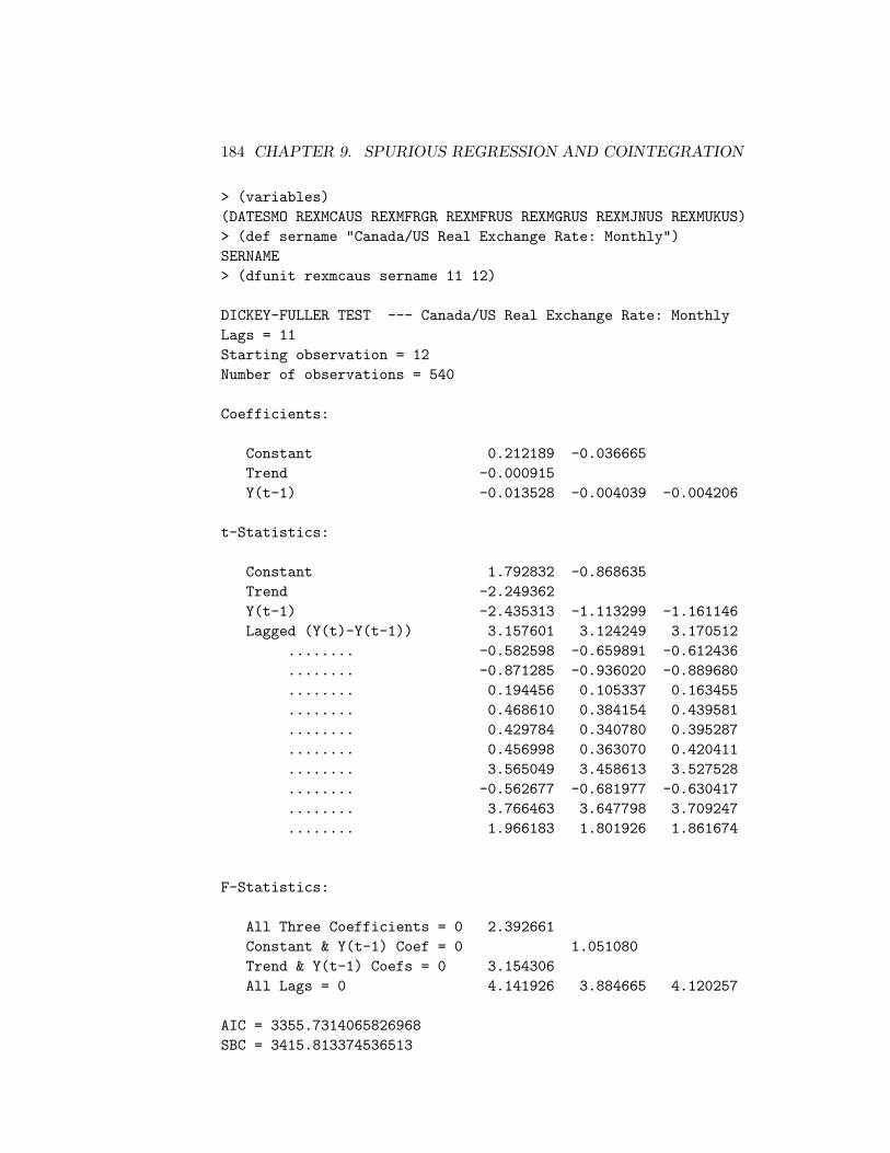
184 CHAPTER 9. SPURIOUS REGRESSION AND COINTEGRATION
> (variables)(DATESMO REXMCAUS REXMFRGR REXMFRUS REXMGRUS REXMJNUS REXMUKUS)> (def sername "Canada/US Real Exchange Rate: Monthly")SERNAME> (dfunit rexmcaus sername 11 12)
DICKEY-FULLER TEST --- Canada/US Real Exchange Rate: MonthlyLags = 11Starting observation = 12Number of observations = 540
Coefficients:
Constant 0.212189 -0.036665Trend -0.000915Y(t-1) -0.013528 -0.004039 -0.004206
t-Statistics:
Constant 1.792832 -0.868635Trend -2.249362Y(t-1) -2.435313 -1.113299 -1.161146Lagged (Y(t)-Y(t-1)) 3.157601 3.124249 3.170512
........ -0.582598 -0.659891 -0.612436
........ -0.871285 -0.936020 -0.889680
........ 0.194456 0.105337 0.163455
........ 0.468610 0.384154 0.439581
........ 0.429784 0.340780 0.395287
........ 0.456998 0.363070 0.420411
........ 3.565049 3.458613 3.527528
........ -0.562677 -0.681977 -0.630417
........ 3.766463 3.647798 3.709247
........ 1.966183 1.801926 1.861674
F-Statistics:
All Three Coefficients = 0 2.392661Constant & Y(t-1) Coef = 0 1.051080Trend & Y(t-1) Coefs = 0 3.154306All Lags = 0 4.141926 3.884665 4.120257
AIC = 3355.7314065826968SBC = 3415.813374536513
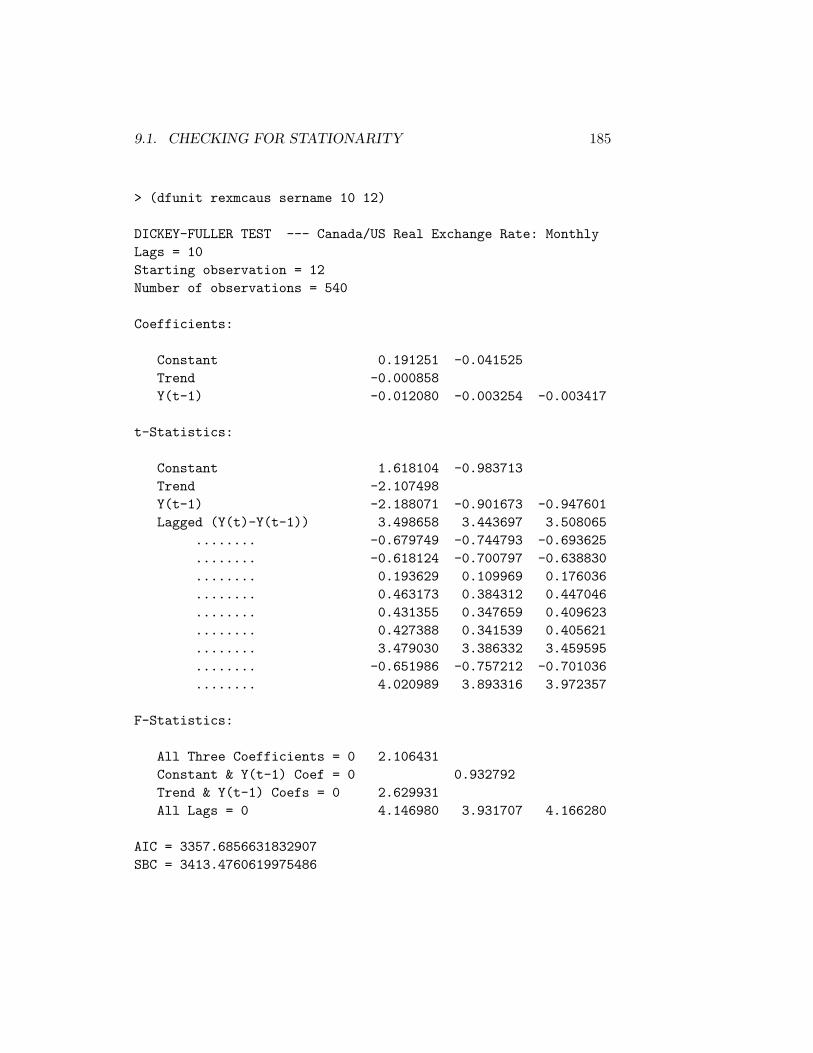
9.1. CHECKING FOR STATIONARITY 185
> (dfunit rexmcaus sername 10 12)
DICKEY-FULLER TEST --- Canada/US Real Exchange Rate: MonthlyLags = 10Starting observation = 12Number of observations = 540
Coefficients:
Constant 0.191251 -0.041525Trend -0.000858Y(t-1) -0.012080 -0.003254 -0.003417
t-Statistics:
Constant 1.618104 -0.983713Trend -2.107498Y(t-1) -2.188071 -0.901673 -0.947601Lagged (Y(t)-Y(t-1)) 3.498658 3.443697 3.508065
........ -0.679749 -0.744793 -0.693625
........ -0.618124 -0.700797 -0.638830
........ 0.193629 0.109969 0.176036
........ 0.463173 0.384312 0.447046
........ 0.431355 0.347659 0.409623
........ 0.427388 0.341539 0.405621
........ 3.479030 3.386332 3.459595
........ -0.651986 -0.757212 -0.701036
........ 4.020989 3.893316 3.972357
F-Statistics:
All Three Coefficients = 0 2.106431Constant & Y(t-1) Coef = 0 0.932792Trend & Y(t-1) Coefs = 0 2.629931All Lags = 0 4.146980 3.931707 4.166280
AIC = 3357.6856631832907SBC = 3413.4760619975486

186 CHAPTER 9. SPURIOUS REGRESSION AND COINTEGRATION
> (dfunit rexmcaus sername 9 12)
DICKEY-FULLER TEST --- Canada/US Real Exchange Rate: MonthlyLags = 9Starting observation = 12Number of observations = 540
Coefficients:
Constant 0.153780 -0.053071Trend -0.000763Y(t-1) -0.009520 -0.001708 -0.001881
t-Statistics:
Constant 1.286792 -1.243797Trend -1.852385Y(t-1) -1.711465 -0.469770 -0.517454Lagged (Y(t)-Y(t-1)) 3.363956 3.320112 3.395934
........ -0.164186 -0.237186 -0.159239
........ -0.627448 -0.700211 -0.621127
........ 0.178872 0.105620 0.189116
........ 0.475189 0.405479 0.485185
........ 0.390381 0.317902 0.395404
........ 0.287053 0.215457 0.293284
........ 3.352378 3.275144 3.362117
........ -0.173654 -0.280887 -0.197184
F-Statistics:
All Three Coefficients = 0 1.751580Constant & Y(t-1) Coef = 0 0.907533Trend & Y(t-1) Coefs = 0 1.826514All Lags = 0 2.732765 2.614381 2.797887
AIC = 3372.0037974689067SBC = 3423.5026271436063
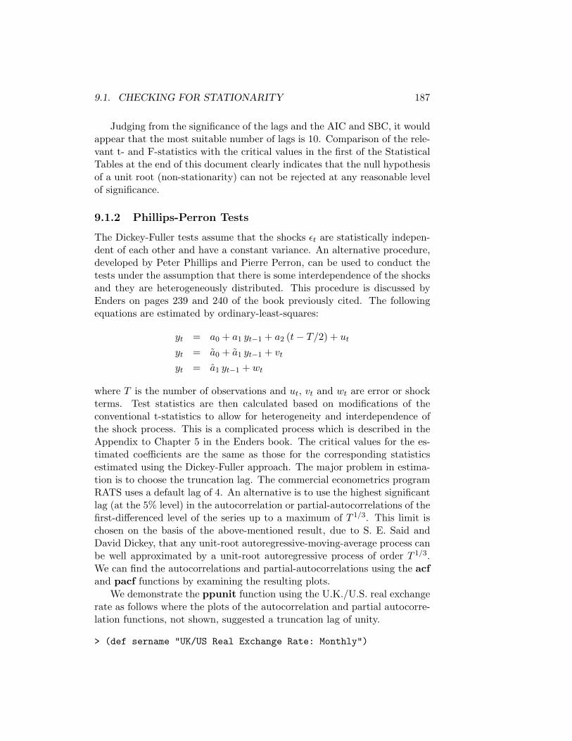
9.1. CHECKING FOR STATIONARITY 187
Judging from the significance of the lags and the AIC and SBC, it wouldappear that the most suitable number of lags is 10. Comparison of the rele-vant t- and F-statistics with the critical values in the first of the StatisticalTables at the end of this document clearly indicates that the null hypothesisof a unit root (non-stationarity) can not be rejected at any reasonable levelof significance.
9.1.2 Phillips-Perron Tests
The Dickey-Fuller tests assume that the shocks εt are statistically indepen-dent of each other and have a constant variance. An alternative procedure,developed by Peter Phillips and Pierre Perron, can be used to conduct thetests under the assumption that there is some interdependence of the shocksand they are heterogeneously distributed. This procedure is discussed byEnders on pages 239 and 240 of the book previously cited. The followingequations are estimated by ordinary-least-squares:
yt = a0 + a1 yt−1 + a2 (t− T/2) + ut
yt = a0 + a1 yt−1 + vt
yt = a1 yt−1 + wt
where T is the number of observations and ut, vt and wt are error or shockterms. Test statistics are then calculated based on modifications of theconventional t-statistics to allow for heterogeneity and interdependence ofthe shock process. This is a complicated process which is described in theAppendix to Chapter 5 in the Enders book. The critical values for the es-timated coefficients are the same as those for the corresponding statisticsestimated using the Dickey-Fuller approach. The major problem in estima-tion is to choose the truncation lag. The commercial econometrics programRATS uses a default lag of 4. An alternative is to use the highest significantlag (at the 5% level) in the autocorrelation or partial-autocorrelations of thefirst-differenced level of the series up to a maximum of T 1/3. This limit ischosen on the basis of the above-mentioned result, due to S. E. Said andDavid Dickey, that any unit-root autoregressive-moving-average process canbe well approximated by a unit-root autoregressive process of order T 1/3.We can find the autocorrelations and partial-autocorrelations using the acfand pacf functions by examining the resulting plots.
We demonstrate the ppunit function using the U.K./U.S. real exchangerate as follows where the plots of the autocorrelation and partial autocorre-lation functions, not shown, suggested a truncation lag of unity.
> (def sername "UK/US Real Exchange Rate: Monthly")

188 CHAPTER 9. SPURIOUS REGRESSION AND COINTEGRATION
SERNAME> (ppunit rexmukus sername 1)
PHILLIPS-PERRON TEST --- UK/US Real Exchange Rate: MonthlyLags Truncated at 1
Least Squares Estimates:
Constant 4.827510E-2 (9.500181E-2)Trend 1.207029E-3 (7.880230E-4)Lagged Y 0.978297 (8.871178E-3)
R Squared: 0.975210Sigma hat: 2.22998Number of cases: 551Degrees of freedom: 548
Standard t-ratios:
Constant 0.5081492680757081Trend 1.5317175364171403Lagged Y = 0 110.27812390482883Lagged Y = 1 -2.4464792798134205
Least Squares Estimates:
Constant 4.907684E-2 (9.511677E-2)Lagged Y 0.987161 (6.731916E-3)
R Squared: 0.975104Sigma hat: 2.23271Number of cases: 551Degrees of freedom: 549
Standard t-ratios:
Constant 0.5159640885651551Lagged Y = 0 146.6389373657781Lagged Y = 1 -1.9071874981089139

9.1. CHECKING FOR STATIONARITY 189
Least Squares Estimates:
Lagged Y 0.987155 (6.727415E-3)
R Squared: 0.975092Sigma hat: 2.23122Number of cases: 551Degrees of freedom: 550
Standard t-ratios:
Lagged Y = 0 146.73622095274848Lagged Y = 1 -1.9092805580788528
PP t-ratio for Coefficient of Lagged Y = 1:-2.781617384738435
PP t-ratio for Constant = 0:0.44550728543536067
PP t-ratio for Trend Coefficient = 0:0.9339088799071322
PP Statistic for Coefficients of Trend = 0 and Lagged Y = 1:3.3165591198878333
PP t-ratio for Coefficient of Lagged Y = 1 in regression without trend:-2.154592593819233
PP t-ratio for Coefficient of Lagged Y = 1 in regression withneither constant nor trend:
-2.158242131639434
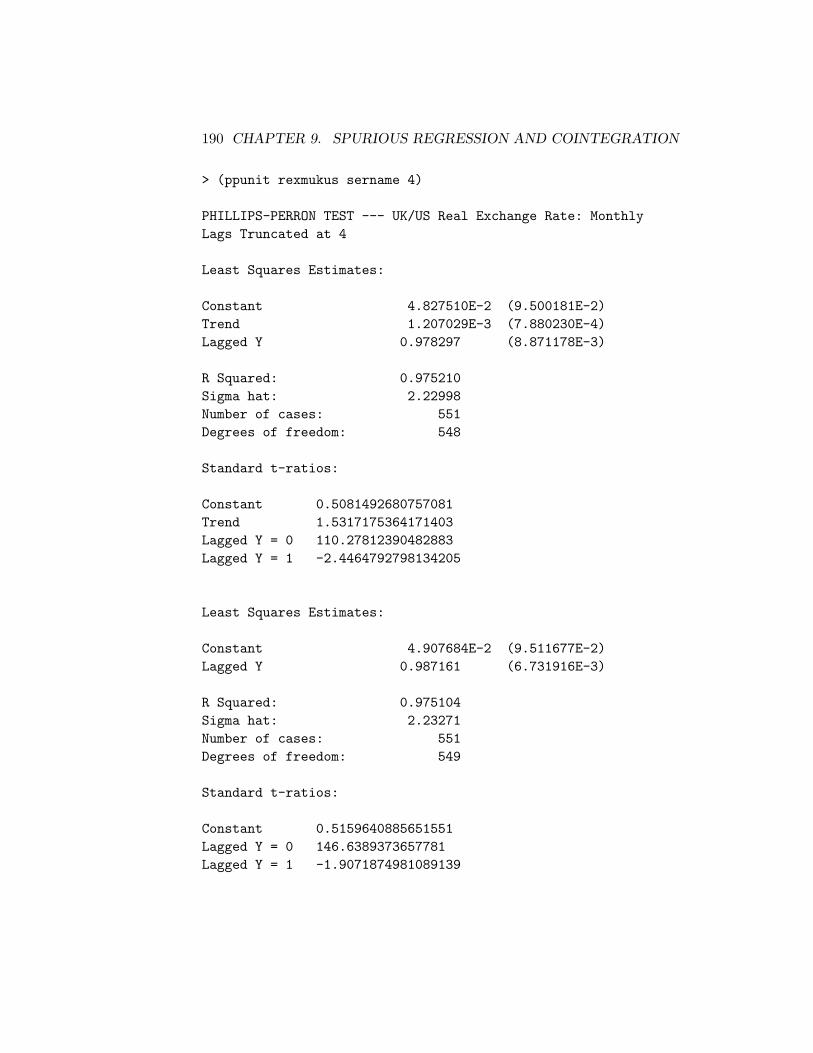
190 CHAPTER 9. SPURIOUS REGRESSION AND COINTEGRATION
> (ppunit rexmukus sername 4)
PHILLIPS-PERRON TEST --- UK/US Real Exchange Rate: MonthlyLags Truncated at 4
Least Squares Estimates:
Constant 4.827510E-2 (9.500181E-2)Trend 1.207029E-3 (7.880230E-4)Lagged Y 0.978297 (8.871178E-3)
R Squared: 0.975210Sigma hat: 2.22998Number of cases: 551Degrees of freedom: 548
Standard t-ratios:
Constant 0.5081492680757081Trend 1.5317175364171403Lagged Y = 0 110.27812390482883Lagged Y = 1 -2.4464792798134205
Least Squares Estimates:
Constant 4.907684E-2 (9.511677E-2)Lagged Y 0.987161 (6.731916E-3)
R Squared: 0.975104Sigma hat: 2.23271Number of cases: 551Degrees of freedom: 549
Standard t-ratios:
Constant 0.5159640885651551Lagged Y = 0 146.6389373657781Lagged Y = 1 -1.9071874981089139
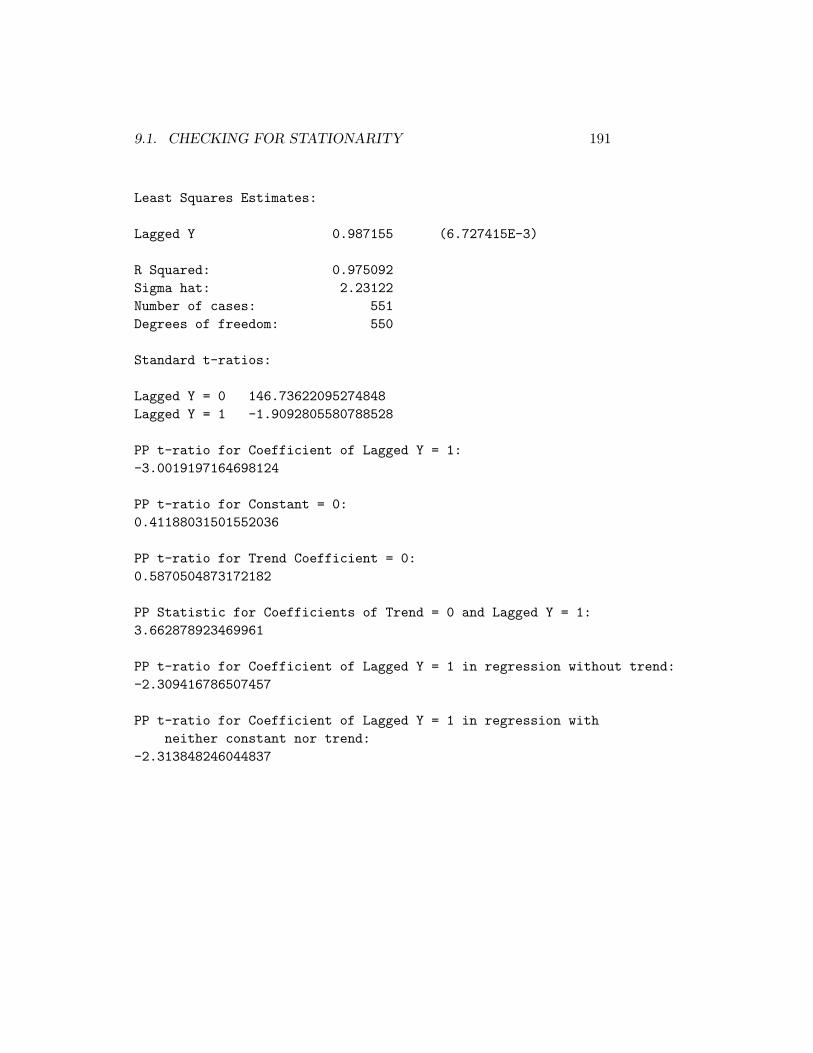
9.1. CHECKING FOR STATIONARITY 191
Least Squares Estimates:
Lagged Y 0.987155 (6.727415E-3)
R Squared: 0.975092Sigma hat: 2.23122Number of cases: 551Degrees of freedom: 550
Standard t-ratios:
Lagged Y = 0 146.73622095274848Lagged Y = 1 -1.9092805580788528
PP t-ratio for Coefficient of Lagged Y = 1:-3.0019197164698124
PP t-ratio for Constant = 0:0.41188031501552036
PP t-ratio for Trend Coefficient = 0:0.5870504873172182
PP Statistic for Coefficients of Trend = 0 and Lagged Y = 1:3.662878923469961
PP t-ratio for Coefficient of Lagged Y = 1 in regression without trend:-2.309416786507457
PP t-ratio for Coefficient of Lagged Y = 1 in regression withneither constant nor trend:
-2.313848246044837

192 CHAPTER 9. SPURIOUS REGRESSION AND COINTEGRATION
9.1.3 The Problem of Low Power
A problem with the above unit-root tests is that they have low power—thatis, they tend to accept the null-hypothesis of non-stationarity too frequentlywhen it is false. For example, suppose that the true coefficient of yt−1 isequal to -.01 in the Dickey-Fuller regressions and .99 in the Phillips-Perronregressions. It will turn out that the corresponding statistics of yt−1 willexceed their 1%, 5%, and 10% critical values only slightly more than 1%,5%, and 10% of the time, respectively. We will reject the null-hypothesisvery rarely, even though it is false. The situation does not get all thatbetter when the respective coefficients of yt−1 are -.05 and -.95, or even -.15 and .85. There will almost surely be a tendency to conclude that theseries in question is non-stationary on occasions, very common in practice,in which it is stationary with very slow mean reversion. This has to be keptin mind when making decisions about whether a series is non-stationary orstationary.
9.2 Testing for Cointegration
Some years ago, it was fashionable to routinely take the first-differences ofnon-stationary series, and then second-differences if the first-difference turnsout to be non-stationary, and then to work with the differenced series. Itis now well-known that such a procedure is inappropriate—by differencingseries, one is throwing away information provided by their levels. Instead,one should check to see if the relevant time series are cointegrated, in whichcase we can do our analysis using OLS regressions of the undifferenced series.
Two or more non-stationary series are cointegrated if a linear combina-tion of them is stationary. For example, consumption and income may bothbe non-stationary but if consumption tends to be a more-or-less constantproportion of income, the two variables are cointegrated—the difference be-tween consumption and income (measured in real terms) or the ratio ofconsumption to income will be stationary processes.2 More generally, aregression of a non-stationary time series on other non-stationary time se-ries will not be spurious if those time series are cointegrated. If they arecointegrated the error-term of the regression will be stationary.
If a non-stationary variable is regressed on stationary variables in ad-dition to non-stationary ones, the coefficients of the stationary variables
2An excellent discussion of these issues can be found on pages 571, 572, and the firsthalf of 573, of James Hamilton’s book Time Series Analysis referenced earlier.

9.2. TESTING FOR COINTEGRATION 193
will always be statistically insignificant if the non-stationary variables arenot cointegrated. But if the non-stationary variables are cointegrated, thestationary variables may well be statistically significant—it will depend onwhether they are correlated with the residual from a linear relationship be-tween the non-stationary variables. If a stationary variable is regressed onnon-stationary variables and the latter are statistically significant, it must bethat those non-stationary variables are cointegrated—the stationary resid-ual from a linear relationship between them is correlated with the stationarydependent variable.
9.2.1 Tests of Regression Residuals for Cointegration
The most obvious way of determining whether a OLS-regression result isspurious is to run a unit-root test on the regression residuals using either orboth of the dfunit or ppunit functions. It turns out that the t-statisticsfrom these regressions follow neither the standard t-distribution nor thedistribution for which Dickey and Fuller calculated the critical values shownin the first table in the Statistical Tables at the end of this document. Theappropriate critical values, calculated by Engle and Yoo and Phillips andOuliaris, can be found in the second table in the Statistical Tables at theend of this document.
These residuals-based cointegration tests are demonstrated below usinga regression of the logarithm of the Canada/United States real exchange rateon the two real variables (of several tried) that survive when HAC coefficient-standard-errors are obtained—the logarithm of an index of U.S. dollar com-modity prices divided by an index of the U.S. dollar prices of U.S. tradedgoods, and the difference between the Canadian and U.S. net capital inflows(calculated as the negatives of the respective trade balances) measured aspercentages of their respective GDPs. The real exchange rate and net capi-tal inflow variables can be shown to be non-stationary using the dfunit andppunit functions while the commodity price variable can be shown to bestationary. The basic regression result is obtained as follows after loadingthe relevant data which is contained in the file rexmdata.lsp.
> (load "addfuncs"); loading addfuncs.lspT> (load "rexqdata"); loading rexqdata.lspT> (variables)(BCOMPXEN DATES72 NGDPCA NGDPUS PCRUDUS PEXPUS PIMPUS REXCAUSTABGSCA TABGSUS)
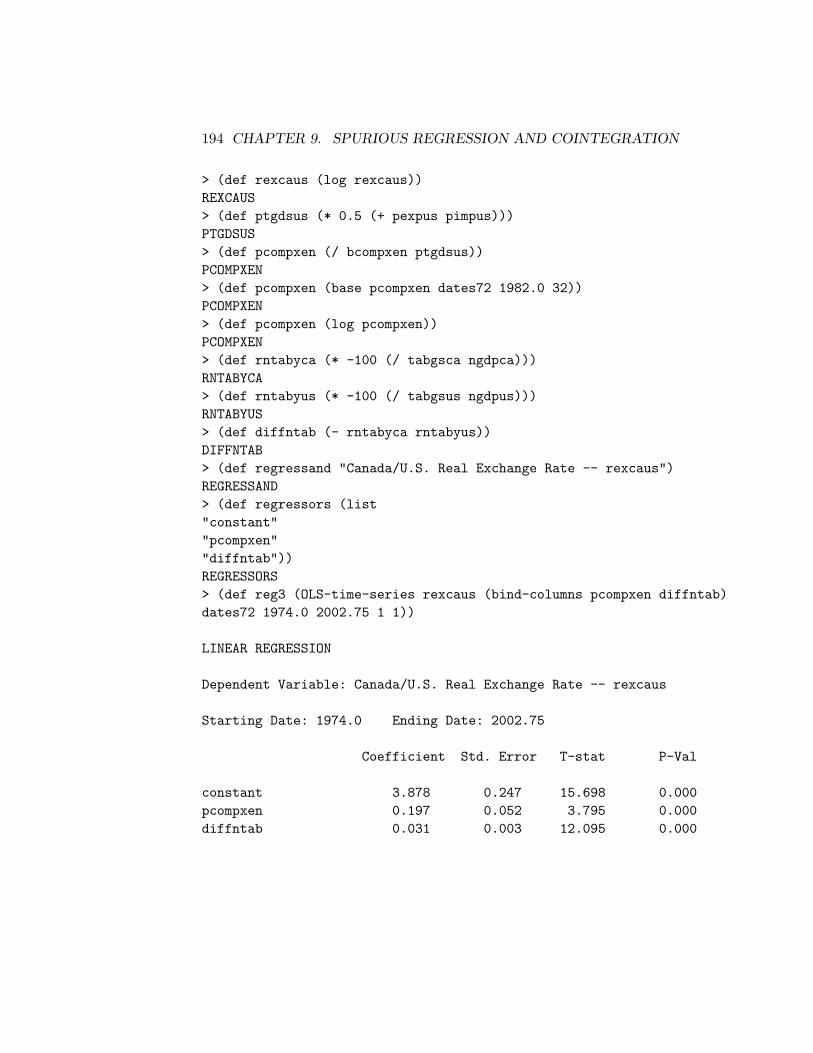
194 CHAPTER 9. SPURIOUS REGRESSION AND COINTEGRATION
> (def rexcaus (log rexcaus))REXCAUS> (def ptgdsus (* 0.5 (+ pexpus pimpus)))PTGDSUS> (def pcompxen (/ bcompxen ptgdsus))PCOMPXEN> (def pcompxen (base pcompxen dates72 1982.0 32))PCOMPXEN> (def pcompxen (log pcompxen))PCOMPXEN> (def rntabyca (* -100 (/ tabgsca ngdpca)))RNTABYCA> (def rntabyus (* -100 (/ tabgsus ngdpus)))RNTABYUS> (def diffntab (- rntabyca rntabyus))DIFFNTAB> (def regressand "Canada/U.S. Real Exchange Rate -- rexcaus")REGRESSAND> (def regressors (list"constant""pcompxen""diffntab"))REGRESSORS> (def reg3 (OLS-time-series rexcaus (bind-columns pcompxen diffntab)dates72 1974.0 2002.75 1 1))
LINEAR REGRESSION
Dependent Variable: Canada/U.S. Real Exchange Rate -- rexcaus
Starting Date: 1974.0 Ending Date: 2002.75
Coefficient Std. Error T-stat P-Val
constant 3.878 0.247 15.698 0.000pcompxen 0.197 0.052 3.795 0.000diffntab 0.031 0.003 12.095 0.000

9.2. TESTING FOR COINTEGRATION 195
Number of Observations: 116Degrees of Freedom: 113R-Squared: 0.7438335246515728Adjusted R-Squared: 0.7392996047339017Sum of Squared Errors: 0.47521761052226746Regression F-Statistic: 164.0596962801281P-Value: 0.0
LM-Based Test for Serial Correlation in Residuals:Order = 1 Chisq-stat = 496.26092143729045 P-Value = 0.0
LM-Based Test for Serial Correlation in Residuals:Order =< 4 Chisq-stat = 515.5116078230459 P-Value = 0.0
LM-Based Test for Serial Correlation in Residuals:Order =< 29 Chisq-stat = 488.9337042721325 P-Value = 0.0
Modified Results Using HAC Standard Errors of Coefficients:Truncation lag = 4
Coefficient Std. Error T-stat P-Val
constant 3.878 0.341 11.372 0.000pcompxen 0.197 0.071 2.787 0.006diffntab 0.031 0.004 8.605 0.000
REG3
We then extract the residuals and perform dfunit and ppunit on them.Since, in Dickey-Fuller unit-root regressions the AIC and SBC were min-imised with no lagged change in residuals, and lagged changes in residualswere statistically insignificant when included, we show below the test withzero lags. The autocorrelation functions and partial autocorrelation func-tions (not shown) indicated no evidence of autocorrelations of the differencedresiduals, we run a Phillips-Perron test for illustrative purposes with one lag.
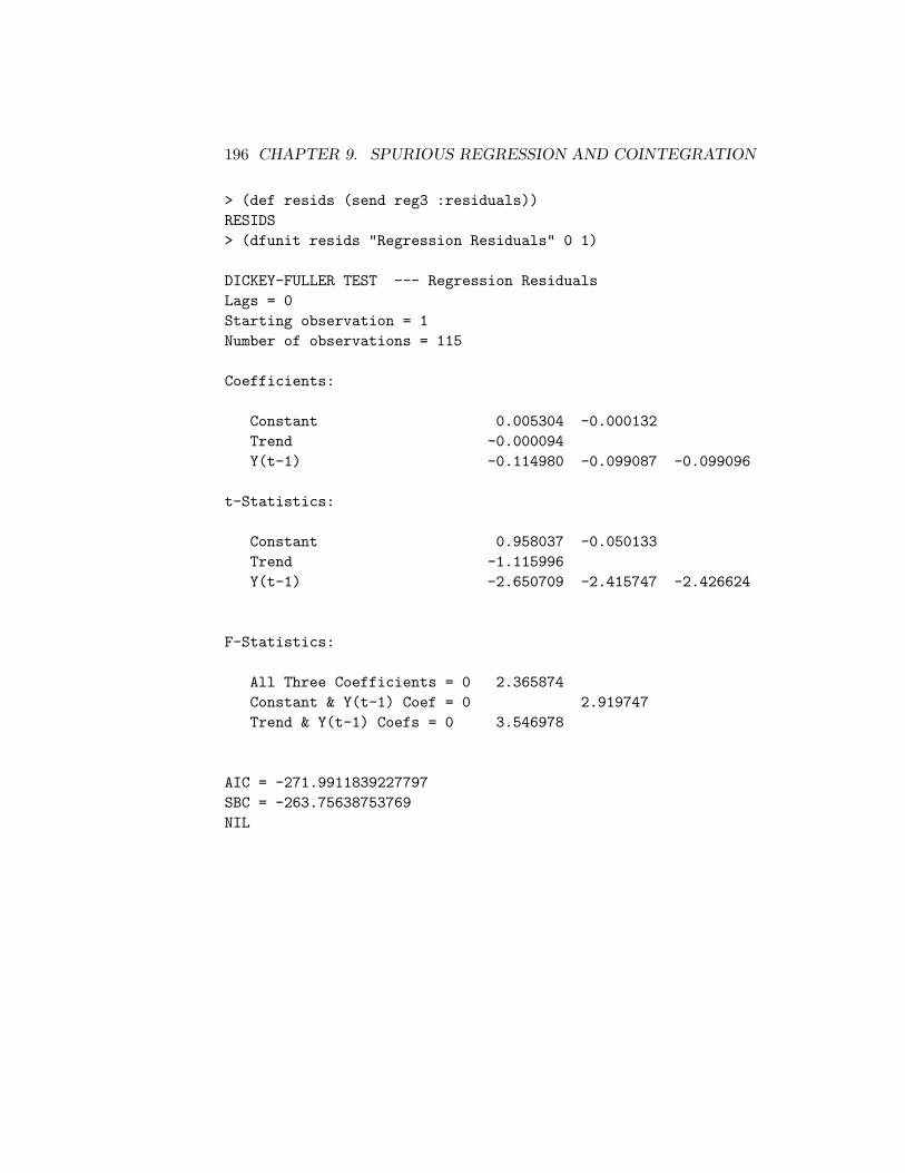
196 CHAPTER 9. SPURIOUS REGRESSION AND COINTEGRATION
> (def resids (send reg3 :residuals))RESIDS> (dfunit resids "Regression Residuals" 0 1)
DICKEY-FULLER TEST --- Regression ResidualsLags = 0Starting observation = 1Number of observations = 115
Coefficients:
Constant 0.005304 -0.000132Trend -0.000094Y(t-1) -0.114980 -0.099087 -0.099096
t-Statistics:
Constant 0.958037 -0.050133Trend -1.115996Y(t-1) -2.650709 -2.415747 -2.426624
F-Statistics:
All Three Coefficients = 0 2.365874Constant & Y(t-1) Coef = 0 2.919747Trend & Y(t-1) Coefs = 0 3.546978
AIC = -271.9911839227797SBC = -263.75638753769NIL
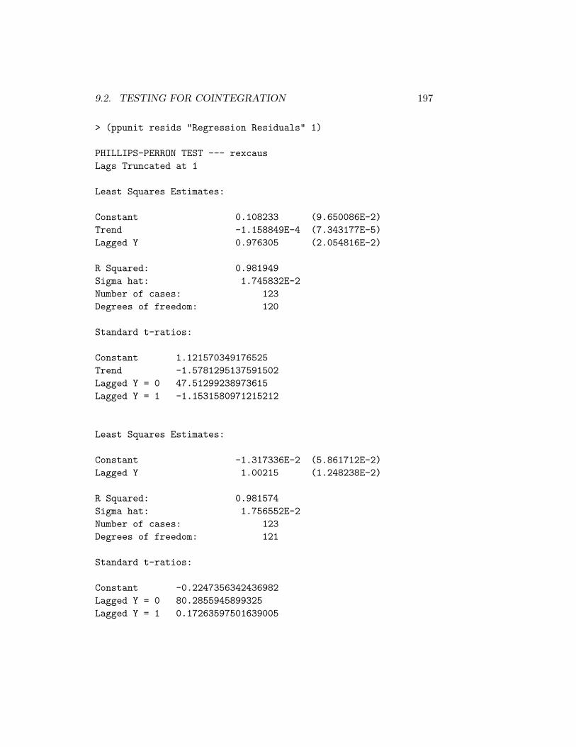
9.2. TESTING FOR COINTEGRATION 197
> (ppunit resids "Regression Residuals" 1)
PHILLIPS-PERRON TEST --- rexcausLags Truncated at 1
Least Squares Estimates:
Constant 0.108233 (9.650086E-2)Trend -1.158849E-4 (7.343177E-5)Lagged Y 0.976305 (2.054816E-2)
R Squared: 0.981949Sigma hat: 1.745832E-2Number of cases: 123Degrees of freedom: 120
Standard t-ratios:
Constant 1.121570349176525Trend -1.5781295137591502Lagged Y = 0 47.51299238973615Lagged Y = 1 -1.1531580971215212
Least Squares Estimates:
Constant -1.317336E-2 (5.861712E-2)Lagged Y 1.00215 (1.248238E-2)
R Squared: 0.981574Sigma hat: 1.756552E-2Number of cases: 123Degrees of freedom: 121
Standard t-ratios:
Constant -0.2247356342436982Lagged Y = 0 80.2855945899325Lagged Y = 1 0.17263597501639005
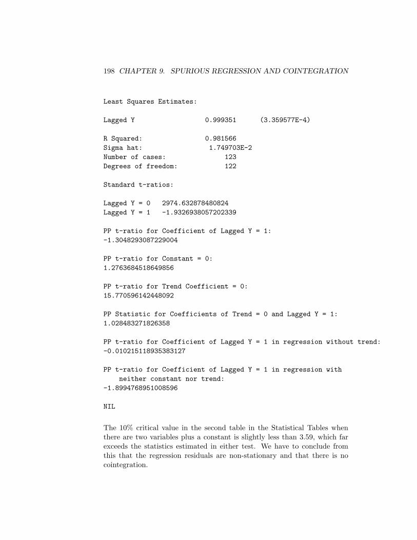
198 CHAPTER 9. SPURIOUS REGRESSION AND COINTEGRATION
Least Squares Estimates:
Lagged Y 0.999351 (3.359577E-4)
R Squared: 0.981566Sigma hat: 1.749703E-2Number of cases: 123Degrees of freedom: 122
Standard t-ratios:
Lagged Y = 0 2974.632878480824Lagged Y = 1 -1.9326938057202339
PP t-ratio for Coefficient of Lagged Y = 1:-1.3048293087229004
PP t-ratio for Constant = 0:1.2763684518649856
PP t-ratio for Trend Coefficient = 0:15.770596142448092
PP Statistic for Coefficients of Trend = 0 and Lagged Y = 1:1.028483271826358
PP t-ratio for Coefficient of Lagged Y = 1 in regression without trend:-0.010215118935383127
PP t-ratio for Coefficient of Lagged Y = 1 in regression withneither constant nor trend:
-1.8994768951008596
NIL
The 10% critical value in the second table in the Statistical Tables whenthere are two variables plus a constant is slightly less than 3.59, which farexceeds the statistics estimated in either test. We have to conclude fromthis that the regression residuals are non-stationary and that there is nocointegration.

9.2. TESTING FOR COINTEGRATION 199
9.2.2 Johansen Cointegration Tests
The problem with the above tests is that they have low power when there issignificant serial correlation, and hence slow mean-reversion, in stationaryregression residuals. An alternative test, developed by Soren Johansen, iscapable of finding cointegration where residual-based tests cannot.3 It isalso capable of finding more than one cointegrating vector with the resultthat the test for cointegration will not hinge on which variable one choosesto be the dependent variable in the cointegrating regression. Johansen’sapproach allows the number of cointegrating relationships equal to as manyas one less than the number of non-stationary variables being analysed.4
The n variables under consideration are expressed as an (n × 1) vectoryt with each variable in the vector expressed as a linear function of laggedvalues of itself and the other variables. The system is written in the form
∆yt = α + ξ0 yt−1 + ξ1 ∆yt−1 + ξ2 ∆yt−1 + · · ·· · ·+ ξp−1 ∆yt−p+1 + εt (9.1)
where α is an n-element column vector of constants, ξ0, ξ1, ξ2, etc., are n×nmatrices of coefficients, and εt is an n-element column vector of residuals.
The number of independent cointegrating vectors is equal to the rank ofthe matrix ξ0 which is in turn equal to the number of its characteristic rootsor eigenvalues that differ from zero.
In performing a Johansen test, the first step is to estimate two sets ofOLS regressions. The first regresses ∆yt on constant terms plus p − 1 ofown lags.
∆yt = φ + Φ1∆yt−1 + Φ2∆yt−2 + · · · · · ·+ Φp−1∆yt−p+1 + ut (9.2)
where the Φi are (n×n) matrices of coefficients and ut is the (n×1) columnvector of OLS residuals. The second set regresses yt on a constant and thesame (p− 1) lags as in the previous regression
yt−1 = θ + Θ1Θyt−1 + Θ2∆yt−2 + · · · · · ·+ Θp−1∆yt−p+1 + vt (9.3)3See Soren Johansen, “Statistical Analysis of Cointegration Vectors,” Journal of Eco-
nomic Dynamics and Control, Vol. 12, 1988, pp. 231-54.4His approach involves full-information maximum likelihood estimation (FIML) of a
system of equations written in vector-autoregressive form. Here we program the cal-culations following the explanation of James Hamilton in Chapter 20 of his previouslyreferenced book Time Series Analysis. For an excellent discussion of the issues involvedin Johansen tests, read pages 385 through 405 of the Enders book Applied Economic TimeSeries referenced earlier. An appropriate review of the basic mathematics issues can befound in the Appendix to the chapter that includes those pages.
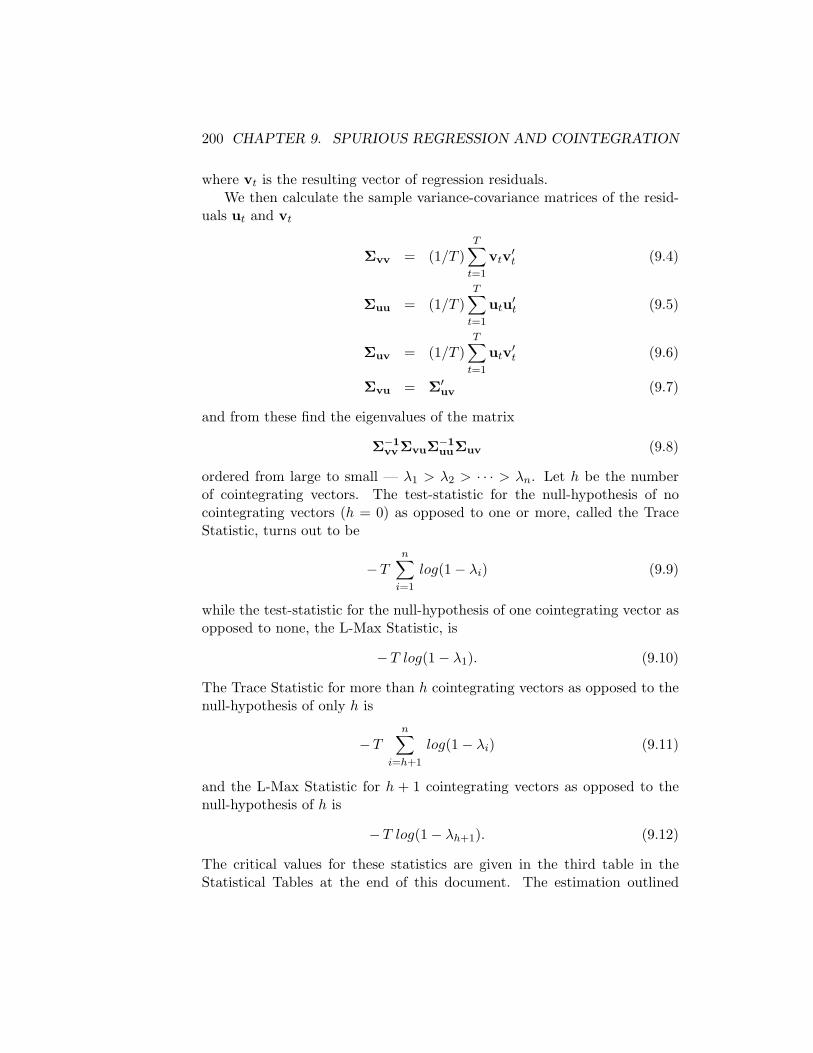
200 CHAPTER 9. SPURIOUS REGRESSION AND COINTEGRATION
where vt is the resulting vector of regression residuals.We then calculate the sample variance-covariance matrices of the resid-
uals ut and vt
Σvv = (1/T )T∑
t=1
vtv′t (9.4)
Σuu = (1/T )T∑
t=1
utu′t (9.5)
Σuv = (1/T )T∑
t=1
utv′t (9.6)
Σvu = Σ′uv (9.7)
and from these find the eigenvalues of the matrix
Σ−1vvΣvuΣ−1
uuΣuv (9.8)
ordered from large to small — λ1 > λ2 > · · · > λn. Let h be the numberof cointegrating vectors. The test-statistic for the null-hypothesis of nocointegrating vectors (h = 0) as opposed to one or more, called the TraceStatistic, turns out to be
−Tn∑
i=1
log(1− λi) (9.9)
while the test-statistic for the null-hypothesis of one cointegrating vector asopposed to none, the L-Max Statistic, is
−T log(1− λ1). (9.10)
The Trace Statistic for more than h cointegrating vectors as opposed to thenull-hypothesis of only h is
−Tn∑
i=h+1
log(1− λi) (9.11)
and the L-Max Statistic for h + 1 cointegrating vectors as opposed to thenull-hypothesis of h is
−T log(1− λh+1). (9.12)
The critical values for these statistics are given in the third table in theStatistical Tables at the end of this document. The estimation outlined

9.2. TESTING FOR COINTEGRATION 201
above allows α to be non-zero so that it is fully compatible with deterministictrend-drift in the data. One could, in addition, restrict the estimation torule out the possibility of deterministic trend-drift, forcing α to be zero.In the above case of unrestricted estimation, the critical values depend onwhether or not there are really deterministic trends in the data—if thereare, the critical values are given in the top panel of the table while if thereare not, the critical values are given in the middle panel.
We can restrict the estimation to exclude deterministic trends by re-peating the above calculations with the constant terms eliminated from thesystem of auxiliary regressions given by equations (9.2) and (9.3).
An alternative restricted estimation is to exclude deterministic trendsfor all the variables but allow constant terms in the cointegrating relations.In this case we have to estimate three auxiliary equations instead of two inthe previous cases. First we estimate equation (9.2) without the constantvector α. Then we regress a constant term on the (p− 1) lags of ∆yt
1 = ω ′1∆yt−1 + ω ′
2∆yt−2 + · · · · · ·+ ω ′p−1∆yt−p+1 + wt. (9.13)
Finally we estimate equation (9.3) without the constant vector θ. Let theresiduals from the first and third regressions be u and v. Then we constructa vector wt equal to the column vector vt with wt added on top of it.
We then calculate the variance-covariance matrices of the residuals
Σww = (1/T )T∑
t=1
wtw′t (9.14)
Σuu = (1/T )T∑
t=1
utu′t (9.15)
Σuw = (1/T )T∑
t=1
utw′t (9.16)
Σwu = Σ′uw (9.17)
and from these find the eigenvalues of the matrix
Σ−1wwΣwuΣ−1
uuΣuw (9.18)
ordered from large to small — λ1 > λ2 > · · · > λn. The Trace and L-Maxstatistics are obtained in the same way as before. In this case, the criticalvalues are in the bottom panel of the third table in the Statistical Tables.They assume that the data conforms to the estimation—that is, no trenddrift but a constant in any cointegrating vector.
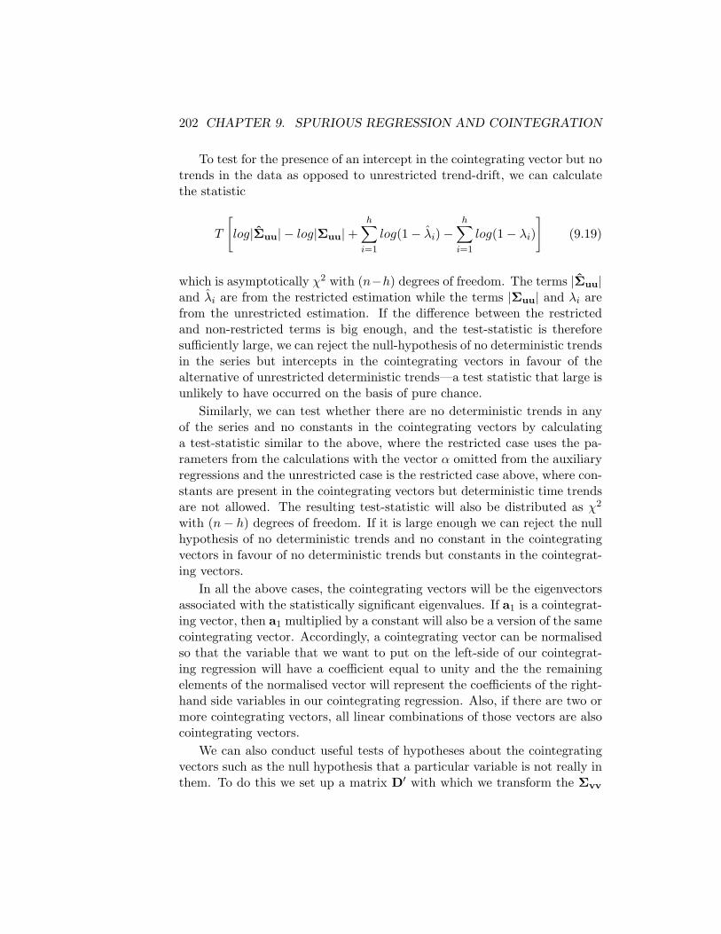
202 CHAPTER 9. SPURIOUS REGRESSION AND COINTEGRATION
To test for the presence of an intercept in the cointegrating vector but notrends in the data as opposed to unrestricted trend-drift, we can calculatethe statistic
T
[log|Σuu| − log|Σuu|+
h∑
i=1
log(1− λi)−h∑
i=1
log(1− λi)
](9.19)
which is asymptotically χ2 with (n−h) degrees of freedom. The terms |Σuu|and λi are from the restricted estimation while the terms |Σuu| and λi arefrom the unrestricted estimation. If the difference between the restrictedand non-restricted terms is big enough, and the test-statistic is thereforesufficiently large, we can reject the null-hypothesis of no deterministic trendsin the series but intercepts in the cointegrating vectors in favour of thealternative of unrestricted deterministic trends—a test statistic that large isunlikely to have occurred on the basis of pure chance.
Similarly, we can test whether there are no deterministic trends in anyof the series and no constants in the cointegrating vectors by calculatinga test-statistic similar to the above, where the restricted case uses the pa-rameters from the calculations with the vector α omitted from the auxiliaryregressions and the unrestricted case is the restricted case above, where con-stants are present in the cointegrating vectors but deterministic time trendsare not allowed. The resulting test-statistic will also be distributed as χ2
with (n− h) degrees of freedom. If it is large enough we can reject the nullhypothesis of no deterministic trends and no constant in the cointegratingvectors in favour of no deterministic trends but constants in the cointegrat-ing vectors.
In all the above cases, the cointegrating vectors will be the eigenvectorsassociated with the statistically significant eigenvalues. If a1 is a cointegrat-ing vector, then a1 multiplied by a constant will also be a version of the samecointegrating vector. Accordingly, a cointegrating vector can be normalisedso that the variable that we want to put on the left-side of our cointegrat-ing regression will have a coefficient equal to unity and the the remainingelements of the normalised vector will represent the coefficients of the right-hand side variables in our cointegrating regression. Also, if there are two ormore cointegrating vectors, all linear combinations of those vectors are alsocointegrating vectors.
We can also conduct useful tests of hypotheses about the cointegratingvectors such as the null hypothesis that a particular variable is not really inthem. To do this we set up a matrix D′ with which we transform the Σvv
9.2. TESTING FOR COINTEGRATION 203
(or Σww) and Σuv (or Σuw) terms as follows,
Σvv = D′ΣvvD (9.20)Σuv = ΣuvD, (9.21)
before combining these and the appropriate Σuu term to calculate the eigen-values. D′ is simply the identity matrix with the row corresponding to thevariable alleged to be missing from the cointegrating vectors deleted. Wethen plug the above-modified matrices and the unrestricted ones into anequivalent of equation (9.19). The resulting test-statistic is χ2 with (n− h)degrees of freedom. If it is high enough, we can reject the null-hypothesisthat the variable in question is not in the cointegrating vector.
To test a relationship between the coefficients of the first and only coin-tegrating vector—for example, that the second two coefficients are both thenegative of the first—we can follow the same procedure as above except thatD′ takes the form (1 -1 -1). This statistic is distributed as χ2 with (n− 1)degrees of freedom. Here, the presence of more than one cointegrating vec-tor would make no sense—we are postulating a specific relationship amongthe variables.
One further issue must be faced before we can proceed to do Johansentests—we must figure out how many lags to include in the basic system(9.1). The common procedure is to estimate the system in the levels (usingundifferenced data) with various lag lengths
yt = a + b1 yt−1 + b2 yt−2 + b3 yt−2 + · · · · · ·+ et (9.22)
and then calculate test-statistics for a Likelihood Ratio test of the form,suggested by Chris Sims,
(T − c)(log|ΣR| − log|ΣU |)
where T is the number of observations, c is the number of parameters inthe unrestricted system (the one including the most lags) and log|ΣR| andlog|ΣU | are the logarithms of determinants of the variance-covariance ma-trices of the residuals in the respective restricted and unrestricted systems.This statistic is distributed as χ2 with degrees of freedom equal to the num-ber of coefficient restrictions. In this case, each lag has n2 coefficients (nlags of n variables) so the number of coefficients will equal m × n2 wherem is the difference in the number of lags of the restricted as opposed tothe unrestricted system. Alternatively, we can select the lag length that
204 CHAPTER 9. SPURIOUS REGRESSION AND COINTEGRATION
minimises the following multivariate generalisation of AIC or SBC.5
AIC = T log|Σ|+ N
SBC = T log|Σ|+ N log(T )
where |Σ| is the variance-covariance matrix of the residuals and N is thenumber of parameters estimated in all equations. The same sample periodmust be used for all systems compared.
To enable a proper choice of lag-length, I have written a function calledVAR-lag-length that takes six arguments in the following order:
—the list of variables—a list of strings giving the names of the above variables—the maximum lag-length—the datelist for the data—the starting date (which must be in the datelist)—the ending date (which must be in the datelist)
The maximum lag-length must not be greater than the excess of the startingdate over the first date in the datelist. This function calculates the statisticalsignificance of each lag in turn, starting from the largest, and calculatesAIC and SBC for each lag-length. All results are printed out. For example,consider the problem of choosing the lag-length for the above analysis of theCanada/U.S. real exchange rate.
> (def varlist (list rexcaus diffntab))VARLIST> (def varnames (list "rexcaus" "diffntab"))VARNAMES
5For a discussion of these issues, see pages 296, 297 and 315 of the Enders book.

9.2. TESTING FOR COINTEGRATION 205
> (VAR-lag-length varlist varnames 8 dates72 1974.0 2002.75)
LAG SELECTION INFORMATION
Variables are (rexcaus diffntab)
Degrees of Freedom Data Points Less LR-TestLag Per Equation All Parameters PVal AIC BIC
8 99 198 -974.58 -880.967 101 202 0.157 -978.23 -895.636 103 206 0.058 -979.70 -908.115 105 210 0.256 -984.63 -924.054 107 214 0.424 -990.73 -941.173 109 218 0.001 -984.56 -946.012 111 222 0.188 -989.00 -961.461 113 226 0.005 -986.06 -969.54
The P-Value is for the restriction of removing the previous lag.
When doing Johansen cointegration tests 2 additional degreesof freedom per equation will be lost, reducing the datapoints minus total parameters estimated by 4
NIL
On the basis of the Likelihood Ratio tests and the AIC, it would appearthat at most 4 lags, and possibly as few as 2, would be appropriate.
We are now in a position to test whether the two non-stationary vari-ables are cointegrated using my Johansen-coint function, which takes thefollowing seven arguments:
—the list of variables—a list of strings giving the names of the above variables—the lag-length—the datelist for the data—the starting date (which must be in the datelist)—the ending date—1 if results are to be printed to screen, 0 otherwise
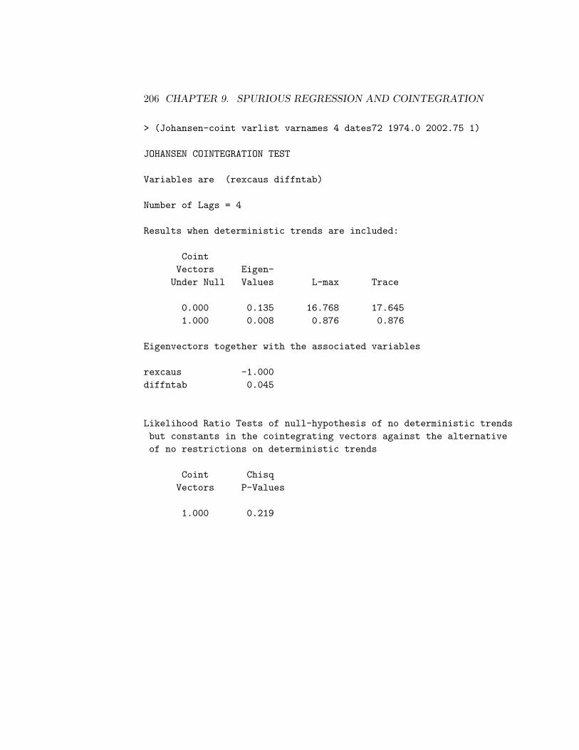
206 CHAPTER 9. SPURIOUS REGRESSION AND COINTEGRATION
> (Johansen-coint varlist varnames 4 dates72 1974.0 2002.75 1)
JOHANSEN COINTEGRATION TEST
Variables are (rexcaus diffntab)
Number of Lags = 4
Results when deterministic trends are included:
CointVectors Eigen-Under Null Values L-max Trace
0.000 0.135 16.768 17.6451.000 0.008 0.876 0.876
Eigenvectors together with the associated variables
rexcaus -1.000diffntab 0.045
Likelihood Ratio Tests of null-hypothesis of no deterministic trendsbut constants in the cointegrating vectors against the alternativeof no restrictions on deterministic trends
Coint ChisqVectors P-Values
1.000 0.219

9.2. TESTING FOR COINTEGRATION 207
Results when deterministic trends are not included and aconstant is present in the cointegrating relationships:
CointVectors Eigen-
Under Null Values L-max Trace
0.000 0.135 16.799 19.1901.000 0.020 2.391 2.391
Eigenvectors together with the associated variables
rexcaus -1.000constant 4.857diffntab 0.045
Likelihood Ratio Tests of null hypothesis of no deterministictrends and no constants in the cointegrating relationshipsversus the alternative of no deterministic trends withconstants in the cointegrating relationships
Coint ChisqVectors P-Values
1.000 0.000

208 CHAPTER 9. SPURIOUS REGRESSION AND COINTEGRATION
Results when deterministic trends are not included and noconstant is present in the cointegrating relationship:
CointVectors Eigen-Under Null Values L-max Trace
0.000 0.027 3.137 3.6961.000 0.005 0.559 0.559
Eigenvectors together with the associated variables
rexcaus -1.000diffntab -0.823
NIL
We can conclude that there are either trends in the data or a constant inthe cointegrating vector, rejecting the null-hypothesis of no trends and noconstant. We cannot reject the presence of a constant in the cointegratingvector with no trends in the data at a reasonable significance level as com-pared to the alternative of unrestricted estimation. In the case where norestrictions are imposed, the Trace statistic of 17.645 and L-max statistic of16.768 both indicate cointegration at the 5% significance level with one coin-tegrating vector if we allow for trend drift in the data. When the estimationrules out trend drift in the data but includes a constant in the cointegratingvector, the Trace and L-max statistics of 19.190 and 16.799, respectively,indicate the presence of one cointegrating vector at about the 5% level. Thenull-hypothesis of no trend-drift in the data and no constant in the cointe-grating vector can clearly be rejected. The issue of whether the individualvariables are present in the cointegrating vector is not of concern—were theynot present, there would be no vector, let alone a cointegrating one.

9.2. TESTING FOR COINTEGRATION 209
As an example of Johansen cointegration tests where hypotheses aretested about the nature of the cointegrating vector, we test the stationarityof the real exchange rate and purchasing-power-parity using Canadian andU.S. monthly data from 1957 through 2002. I wrote the function Johansen-cointvector-test for this purposes. The function takes two arguments—first the D matrix defined above and second, 1 if the result is to be printed or0 otherwise. Three variables enter the test—the Canadian CPI, the nominalexchange rate expressed as the U.S. dollar price of the Canadian dollar andthe U.S. CPI. The data are in the files nexmdata.lsp and cpimdata.lsp.Stationarity of the real exchange rate requires that these three variables becointegrated, and purchasing-power-parity requires that the logarithms ofthe three variables enter the cointegrating vector with coefficients propor-tional to 1, -1 and 1, respectively. The results are as follows.
> (load "addfuncs"); loading addfuncs.lspT> (load "nexmdata"); loading nexmdata.lspT> (load "cpimdata"); loading cpimdata.lspT> (variables)(CPIMCA CPIMFR CPIMGR CPIMJN CPIMUK CPIMUS DATESMO NEXMCANEXMFR NEXMGR NEXMJN NEXMUK)> (def nexmca (/ 1 nexmca))NEXMCA> (def cpica (log cpimca))CPICA> (def cpius (log cpimus))CPIUS> (def nexca (log nexmca))NEXCA> (def varlist (list cpica nexca cpius))VARLIST> (def varnames (list "cpica" "nexca" "cpius"))VARNAMES

210 CHAPTER 9. SPURIOUS REGRESSION AND COINTEGRATION
> (VAR-lag-length varlist varnames 30 datesmo 1960.0 2002.915)
LAG SELECTION INFORMATION
Variables are (cpica nexca cpius)
Degrees of Freedom Data Points Less LR-TestLag Per Equation All Parameters PVal AIC BIC
30 425 1275 -17026.88 -15867.6929 428 1284 0.002 -17027.26 -15906.2928 431 1293 0.192 -17039.54 -15956.7927 434 1302 0.001 -17037.16 -15992.6226 437 1311 0.056 -17046.15 -16039.8225 440 1320 0.041 -17054.41 -16086.3024 443 1329 0.000 -17049.81 -16119.9123 446 1338 0.250 -17063.03 -16171.3522 449 1347 0.021 -17069.78 -16216.3121 452 1356 0.004 -17072.55 -16257.3020 455 1365 0.100 -17083.42 -16306.3919 458 1374 0.017 -17089.91 -16351.0818 461 1383 0.016 -17096.25 -16395.6417 464 1392 0.290 -17110.06 -16447.6616 467 1401 0.002 -17111.09 -16486.9115 470 1410 0.012 -17116.95 -16530.9814 473 1419 0.007 -17121.64 -16573.9013 476 1428 0.003 -17124.41 -16614.8812 479 1437 0.000 -17082.48 -16611.1611 482 1446 0.000 -17069.93 -16636.8210 485 1455 0.000 -17056.79 -16661.909 488 1464 0.000 -17044.39 -16687.728 491 1473 0.000 -17040.97 -16722.527 494 1482 0.013 -17047.58 -16767.346 497 1491 0.057 -17057.73 -16815.705 500 1500 0.000 -17047.68 -16843.864 503 1509 0.000 -17043.64 -16878.043 506 1518 0.000 -17035.67 -16908.292 509 1527 0.000 -17016.27 -16927.101 512 1536 0.000 -16772.36 -16721.41
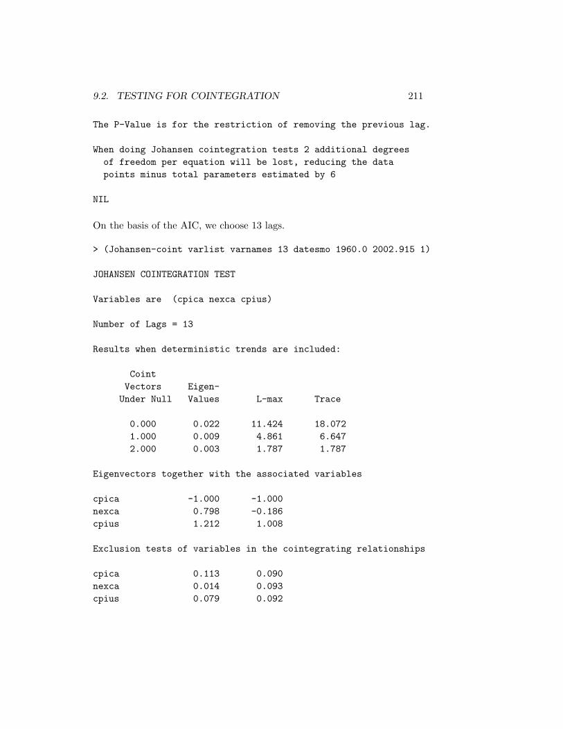
9.2. TESTING FOR COINTEGRATION 211
The P-Value is for the restriction of removing the previous lag.
When doing Johansen cointegration tests 2 additional degreesof freedom per equation will be lost, reducing the datapoints minus total parameters estimated by 6
NIL
On the basis of the AIC, we choose 13 lags.
> (Johansen-coint varlist varnames 13 datesmo 1960.0 2002.915 1)
JOHANSEN COINTEGRATION TEST
Variables are (cpica nexca cpius)
Number of Lags = 13
Results when deterministic trends are included:
CointVectors Eigen-
Under Null Values L-max Trace
0.000 0.022 11.424 18.0721.000 0.009 4.861 6.6472.000 0.003 1.787 1.787
Eigenvectors together with the associated variables
cpica -1.000 -1.000nexca 0.798 -0.186cpius 1.212 1.008
Exclusion tests of variables in the cointegrating relationships
cpica 0.113 0.090nexca 0.014 0.093cpius 0.079 0.092

212 CHAPTER 9. SPURIOUS REGRESSION AND COINTEGRATION
Likelihood Ratio Tests of null hypothesis of no deterministic trendsbut constants in the cointegrating vectors against the alternativeof no restrictions on deterministic trends
Coint ChisqVectors P-Values
1.000 0.1222.000 0.153
Results when deterministic trends are not included and con-stants are present in the cointegrating relationships:
CointVectors Eigen-Under Null Values L-max Trace
0.000 0.023 12.230 23.0841.000 0.014 7.022 10.8542.000 0.007 3.831 3.831
Eigenvectors together with the associated variables
cpica -1.000 -1.000constant -0.724 -0.372nexca 0.986 0.063cpius 1.242 1.080
Exclusion tests of variables in the cointegrating relationships
constant 0.075 0.087cpica 0.239 0.115nexca 0.023 0.106cpius 0.187 0.103

9.2. TESTING FOR COINTEGRATION 213
Likelihood Ratio Tests of null hypothesis of no deterministictrends and no constants in the cointegrating relationshipsversus the alternative of no deterministic trends withconstants in the cointegrating relationships
Coint ChisqVectors P-Values
1.000 0.0012.000 0.002
Results when deterministic trends are not included and noconstant is present in the cointegrating relationship:
CointVectors Eigen-
Under Null Values L-max Trace
0.000 0.017 9.068 13.4581.000 0.008 4.096 4.3902.000 0.001 0.294 0.294
Eigenvectors together with the associated variables
cpica -1.000 -1.000nexca -1.207 -0.072cpius 0.882 0.995
Exclusion tests of variables in the cointegrating relationships
cpica 0.452 0.059nexca 0.034 0.420cpius 0.499 0.059
NIL

214 CHAPTER 9. SPURIOUS REGRESSION AND COINTEGRATION
> (def D (bind-columns (list 1 -1 1)))D> (Johansen-cointvector-test D 1)
D matrix
1.000-1.0001.000
Chisquare Statistic = 9.293670058789424
P-Value = 0.009591912059625507
NIL
It is obvious from a glance at the third row of any of the three panels in thethird of our Statistical Tables that no cointegrating relationship holds, im-plying what we knew previously—that the Canadian real exchange rate withrespect to the United States is non-stationary. And, not surprisingly, thenull-hypothesis implying purchasing-power-parity is clearly rejected. Wereit not for purposes of illustration, there would have been no point in runningthe Johansen-cointvector-test function.

Chapter 10
Further Topics in RegressionAnalysis
We now explore a number of further issues in the application of regressionanalysis to economics. First, we extend the testing of joint hypotheses be-yond the ‘rule of thumb’ F-tests outlined in the multicollinearity section ofChapter 5. Then we outline some non-nested hypotheses tests that can en-able us to distinguish between two competing theories explaining observedbehaviour of economic variables. Our third topic is generalised least squares,which we introduce with an analysis of traditional ways of dealing with serialcorrelation in time-series residuals. Finally, we apply these GLS principlesto the use of seemingly unrelated regression techniques in analysing a systemof equations.
10.1 Joint Hypotheses Tests
In Chapter 5 we showed that a general hypothesis about the coefficientsin a linear regression can be tested by running the regression with andwithout imposing the implied constraints and then running an F-test onthe difference between the sum-of-squared residuals in the two cases. Theresulting F-statistic was
F =(SSER− SSEU)/q
SSEU/DFU
where SSER and SSEU are the restricted and unrestricted sum of squaredregression residuals, q is the number of restrictions (degrees of freedom in thenumerator) and DFU is the degrees of freedom in the unrestricted regression
215
216 CHAPTER 10. FURTHER TOPICS IN REGRESSION ANALYSIS
(and in the denominator). One of the difficulties with this ‘rule of thumb’F-test is that it does not accommodate adjustment for heteroskedasticityand autocorrelation in the regression residuals.
An alternative approach is to express the restriction or set of joint re-strictions in the following matrix form
Rβ = r
where R is a matrix whose rows are represented by the individual restrictionsand whose columns equal the number of regressors including the constant,r is a column vector equal in length to the number of restrictions and,hence to the number of rows in R, and β is the vector of coefficients of theunrestricted regression. The F-statistic, identical to the one above in thecases where the errors are homoskedastic, can then be expressed as
F = (Rβ − r)′[RΣR′]−1(Rβ − r)/q
where Σ is the variance-covariance matrix of the coefficients in the unre-stricted regression. These variances and covariances may or may not beadjusted to accommodate heteroskedasticity and autocorrelation in the re-gression residuals, as the situation requires. In the case where the regressionresiduals are homoskedastic, Σ = σ2I, where I is the identity matrix andthe denominator becomes identical to that in the previous ‘rule of thumb’F-statistic. The numerators are also identical, but that fact is not obvious.
When the restriction being tested is simply that the coefficient of thesecond variable is zero in a regression that has, say, three variables plus aconstant term, R and r become
R = [0 1 0 0] and r = 0
and in the case where the restriction is that the second and third coefficientsare equal they become
R = [0 1 -1 0] and r = 0.
In a test of the significance of the regression—that is, of the null-hypothesisthat all coefficients except that of the constant term are jointly zero—R andr become
R =
0 1 0 00 0 1 00 0 0 1
and r =
000
.

10.1. JOINT HYPOTHESES TESTS 217
The null-hypothesis is that R post-multiplied by the four-element columnvector β equals r—that is, β2 = 0 in the first case above, β2 = β3 in thesecond case and in the last case, β2 = β3 = β4 = 0.
To apply the above methods we use a data set collected by my latecolleague Trevor Dick, used in our joint working paper “Capital Imports andthe Jacksonian Economy: A New View of the Balance of Payments” whichstudied the operation of the bi-metallic gold/silver and gold standards in theUnited States during the period 1820 through 1860.1 The data, containedin the file antbdata.lsp, can be described as follows, where ROW refers tothe rest of the world:2
YEAR — 1820 through 1860USTOTN —US terms of trade, 1850 = 100USROWRN —US/ROW non-traded goods price index, 1850 = 1000USCPIBDS —US CPI, 1850 = 100ROWPL —Rest of world price level, 1850 = 100
(ROW = UK, France, Germany and Sweden)NPRUSROW —US/ROW price level USCPIBDS/ROWPL
equals a real exchange rate estimateREXUSROW —US/ROW price level and real exchange rate
based on USIPDB/ROWPLROWRGNP —Rest of world real GNPUSNGNPB —US nominal GNPUSRGNPB —US real GNPUSRGNPBI —US real GNP – Index 1850 = 100USIPDB —US implicit GNP deflator, 1850 = 100USRDSB —US real debt service balance – using USCPIBDSUSRPLS —US real public land sales in thous. of 1850 dollarsUSRCANI —US real canal investment in mill. of 1850 dollarsUSRRMP —US railroad mileage – = zero to 1830USTBN —US balance of trade in goods and services in mill. curr. $USSERV —US service balance excluding services of capitalUSTBNGS —US balance of trade in goods and services excluding
the services of capital – mill. current $USTBRGS —US real balance of trade in goods and services
excluding the services of capital –mill. 1850 $
1The on-line version of this paper can be obtained athttp://www.economics.utoronto.ca/ecipa/archive/UT-ECIPA-FLOYD-01-01.html.
2These data are a subset of the full data set available, along with other data collectedby Trevor Dick, at
http://www.economics.utoronto.ca/floyd/dick.html .

218 CHAPTER 10. FURTHER TOPICS IN REGRESSION ANALYSIS
USNCIDSB —US real net capital inflow plus DSB = USTBNGS/USIPDBmillions of 1850 dollars
UKOMDR —UK open market discount rateUKCONSOL —UK consol rateUSSINT —US short-term interest rate – based on several seriesINTDIF —US/UK interest rate differential — USSINT/UKOMDRUSSPTC —Specie stock in US in millions of current dollarsNRESFLOW —Nominal flow of reserves into the US – USSPTC(T)-USSPTC(T-1)RRESFLOW —Real flow of reserves into the US evaluated at T-1
prices – = 100*NRESFLOW(T)/USCPIBDS(T-1)USMONT —US money stock in millions of current dollarsUSRMON —US real money stock in 1850 dollars — USMONT/USCPIBDSUSRSPRES —US real stock of specie reserves – millions 1850 $
= 100* USSPTC/USCPIBDSUSMM —US money multiplier – USMONT/USSPTCUSRNCIXS —US real net capital imports less specie exportsUSSPECXP —US specie exports – mill. of current dollarsUSUKMPO —US dollar / Sterling mint parity in $ per poundUSUKEXRB —Anglo-American nominal exchange rate – estimate 1USUKEXRP —Anglo-American nominal exchange rate – estimate 2
We can now bring these data into the XLispStat workspace.
> (load "addfuncs.lsp"); loading addfuncs.lspT> (load "antbdata.lsp"); loading antbdata.lspT> (variables)(INTDIF NPRUSROW NRESFLOW REXUSROW ROWPL ROWRGNP RRESFLOWUKCONSOL UKOMDR USCPIBDS USIPDB USMM USNCIDSB USNGNPBUSNMONT USRCANI USRDSB USRGNPB USRGNPBI USRMON USRNCIXSUSROWRN USRPLS USRRMP USRSPRES USSERV USSINT USSPECXP USSPTCUSTBN USTBNGS USTBRGS USTOTN USUKEXRB USUKEXRP USUKMPO YEAR)
We begin the analysis by setting up a reduced form estimating equationto explain movements in the U.S. real balance of trade in goods and servicesduring the period. The obvious explanatory variables are real incomes inthe U.S. and the rest of the world and the U.S. real exchange rate withrespect to the rest of the world. Additional potential regressors are the debt
10.1. JOINT HYPOTHESES TESTS 219
service balance, changes in which will cause U.S. relative to foreign incomesto change in ways that might not entirely be captured by our U.S. andrest-of-world real income variables, and various factors affecting long-termreal net capital inflows which we proxy by real public land sales, real canalinvestment and railroad mileage. Of course, these real net capital inflowswill only cause the real trade balance to change at a given real exchangerate if they happen to be accompanied by shifts in the supply relative tothe demand of actual real capital goods—otherwise, the real exchange ratewill adjust until the current account deficit equals the net capital inflow.The estimated equation is a reduced form because, although it might bereasonable to expect a negative relationship between the real trade balanceand the real exchange rate, the observed relationship will undoubtedly sufferfrom simultaneity bias and need not even be negative. The reason is thatswings in the demand for U.S. exports relative to imports will cause realexchange rate movements that may be unrelated to changes in the realtrade balance, since the latter must be equal to the negative of the real netcapital inflow, which will change only if there are changes in U.S. investmentrelative to savings.3
We use a measure of the real exchange rate that, given the fixed nom-inal exchange rate implied by the fixing of the values of the domestic andforeign currencies in terms of silver and gold, matches the movement of theU.S. implicit GNP deflator relative to the rest-of-world price level. Thiscontrasts with the working paper where the U.S. consumer price index wasused instead of the GNP deflator. The change is made because it favoursthe theory which the working paper cited and our analysis here ultimatelyrejects.
> (def regressand "Real Trade Balance")REGRESSAND> (def regressors (list "Constant " "Real Exch Rate" "US Real Income""ROW Real Income" "Pub Land Sales" "Canal Inv" "Rail Mileage" "Net RepEarn"))REGRESSORS> (def idepvars (bind-columns rexusrow usrgnpbi rowrgnp usrpls usrcaniusrrmp usrdsb))IDEPVARS
3For a discussion of the important analytical economic issues involved here, see sectionfour of the Dick-Floyd working paper cited above.
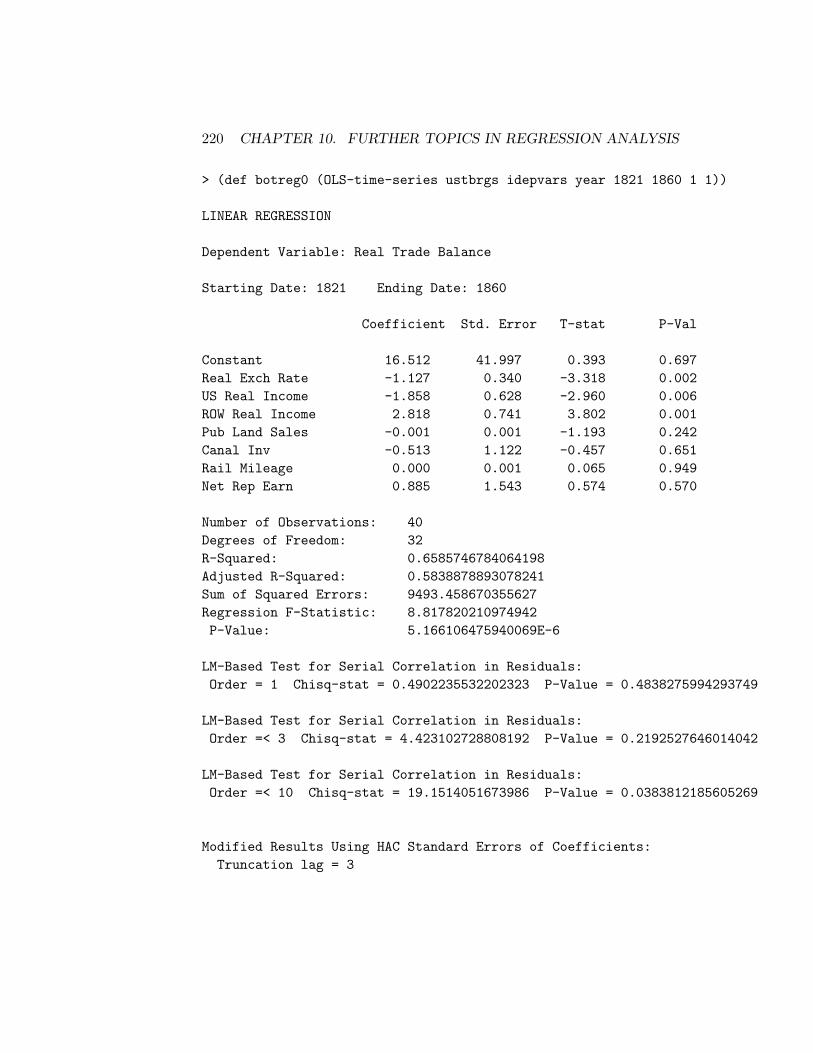
220 CHAPTER 10. FURTHER TOPICS IN REGRESSION ANALYSIS
> (def botreg0 (OLS-time-series ustbrgs idepvars year 1821 1860 1 1))
LINEAR REGRESSION
Dependent Variable: Real Trade Balance
Starting Date: 1821 Ending Date: 1860
Coefficient Std. Error T-stat P-Val
Constant 16.512 41.997 0.393 0.697Real Exch Rate -1.127 0.340 -3.318 0.002US Real Income -1.858 0.628 -2.960 0.006ROW Real Income 2.818 0.741 3.802 0.001Pub Land Sales -0.001 0.001 -1.193 0.242Canal Inv -0.513 1.122 -0.457 0.651Rail Mileage 0.000 0.001 0.065 0.949Net Rep Earn 0.885 1.543 0.574 0.570
Number of Observations: 40Degrees of Freedom: 32R-Squared: 0.6585746784064198Adjusted R-Squared: 0.5838878893078241Sum of Squared Errors: 9493.458670355627Regression F-Statistic: 8.817820210974942P-Value: 5.166106475940069E-6
LM-Based Test for Serial Correlation in Residuals:Order = 1 Chisq-stat = 0.4902235532202323 P-Value = 0.4838275994293749
LM-Based Test for Serial Correlation in Residuals:Order =< 3 Chisq-stat = 4.423102728808192 P-Value = 0.2192527646014042
LM-Based Test for Serial Correlation in Residuals:Order =< 10 Chisq-stat = 19.1514051673986 P-Value = 0.0383812185605269
Modified Results Using HAC Standard Errors of Coefficients:Truncation lag = 3

10.1. JOINT HYPOTHESES TESTS 221
Coefficient Std. Error T-stat P-Val
Constant 16.512 31.234 0.529 0.601Real Exch Rate -1.127 0.216 -5.205 0.000US Real Income -1.858 0.590 -3.150 0.004ROW Real Income 2.818 0.617 4.567 0.000Pub Land Sales -0.001 0.000 -2.554 0.016Canal Inv -0.513 0.646 -0.793 0.434Rail Mileage 0.000 0.001 0.080 0.936Net Rep Earn 0.885 1.456 0.608 0.548
BOTREG0
It is interesting to note that the test routine of our OLS-time-series func-tion found evidence of only high-order serial correlation in the regressionresiduals. The results also indicate that the debt service balance (net repa-triated earnings) and all the proxies for long-term real capital growth exceptpublic land sales are individually not statistically significant. We thereforedo a joint hypothesis test of whether they are significant as a group. Firstwe create the R matrix and the column vector r and then use the joint-hypothesis-test function that I wrote to use these objects along with thevariance-covariance matrix of the coefficients to calculate the F-statistic.The function takes only two arguments, the regression-model object and acoefficient that determines whether HAC standard errors are used. It takesa value of -1 in the homoskedastic case, 0 when there is adjustment for het-eroskedasticity alone and a positive value equal to the number of lags whenthe adjustment is for autocorrelation as well as heteroskedasticity. The num-ber of restrictions, q, is automatically obtained from the length of the vectorr. In the homoskedastic case the function delivers an F-statistic while withHAC coefficient standard errors it produces a χ2 statistic, which is equal toq times the Fq,∞ statistic.
> (def bigr (bind-rows (list 0 0 0 0 0 1 0 0)))BIGR> (def bigr (bind-rows bigr (list 0 0 0 0 0 0 1 0)))BIGR> (def bigr (bind-rows bigr (list 0 0 0 0 0 0 0 1)))BIGR> (def litr (bind-columns (repeat 0 3)))LITR

222 CHAPTER 10. FURTHER TOPICS IN REGRESSION ANALYSIS
> (joint-hypothesis-test botreg0 -1)
Joint Hypothesis Significance Test
R =0.000 0.000 0.000 0.000 0.000 1.000 0.000 0.0000.000 0.000 0.000 0.000 0.000 0.000 1.000 0.0000.000 0.000 0.000 0.000 0.000 0.000 0.000 1.000
r =0.0000.0000.000
F-Statistic = 0.2812963619298308P-Value = 0.8384901630007598
NIL
It turns out that the above variables plus public land sales are as a group alsoinsignificant except when HAC coefficient standard errors are incorporated.
> (def bigr (bind-rows (list 0 0 0 0 1 0 0 0)))BIGR> (def bigr (bind-rows bigr (list 0 0 0 0 0 1 0 0)))BIGR> (def bigr (bind-rows bigr (list 0 0 0 0 0 0 1 0)))BIGR> (def bigr (bind-rows bigr (list 0 0 0 0 0 0 0 1)))BIGR> (def litr (bind-columns (repeat 0 4)))LITR> (joint-hypothesis-test botreg0 -1)
Joint Hypothesis Significance Test
R =0.000 0.000 0.000 0.000 1.000 0.000 0.000 0.0000.000 0.000 0.000 0.000 0.000 1.000 0.000 0.0000.000 0.000 0.000 0.000 0.000 0.000 1.000 0.0000.000 0.000 0.000 0.000 0.000 0.000 0.000 1.000

10.1. JOINT HYPOTHESES TESTS 223
r =0.0000.0000.0000.000
F-Statistic = 0.8103204407983537P-Value = 0.5278954330345068
NIL> (joint-hypothesis-test botreg0 3)
Joint Hypothesis Significance Test
R =0.000 0.000 0.000 0.000 1.000 0.000 0.000 0.0000.000 0.000 0.000 0.000 0.000 1.000 0.000 0.0000.000 0.000 0.000 0.000 0.000 0.000 1.000 0.0000.000 0.000 0.000 0.000 0.000 0.000 0.000 1.000
r =0.0000.0000.0000.000
Chisquare Statistic = 14.47502000468472P-Value = 0.005923594186175163
NIL
When rerun the regression including Public Land Sales but omitting theother insignificant variables, the Public Land Sales variable turns out to bestatistically insignificant with no serial correlation present in the residuals.Accordingly, we then drop that variable as well.4
4All these results are programmed in the batch file JHTbatch.lsp.
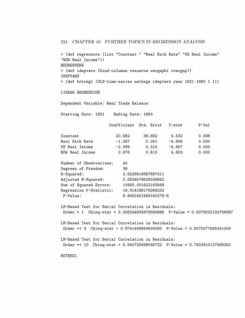
224 CHAPTER 10. FURTHER TOPICS IN REGRESSION ANALYSIS
> (def regressors (list "Constant " "Real Exch Rate" "US Real Income""ROW Real Income"))REGRESSORS> (def idepvars (bind-columns rexusrow usrgnpbi rowrgnp))IDEPVARS> (def botreg1 (OLS-time-series ustbrgs idepvars year 1821 1860 1 1))
LINEAR REGRESSION
Dependent Variable: Real Trade Balance
Starting Date: 1821 Ending Date: 1860
Coefficient Std. Error T-stat P-Val
Constant 20.682 38.882 0.532 0.598Real Exch Rate -1.267 0.261 -4.858 0.000US Real Income -2.099 0.315 -6.657 0.000ROW Real Income 2.976 0.613 4.853 0.000
Number of Observations: 40Degrees of Freedom: 36R-Squared: 0.6239916887697411Adjusted R-Squared: 0.5926576628338862Sum of Squared Errors: 10455.051622163568Regression F-Statistic: 19.914188175089233P-Value: 8.848164156916027E-8
LM-Based Test for Serial Correlation in Residuals:Order = 1 Chisq-stat = 0.008244934976584888 P-Value = 0.9276502193756687
LM-Based Test for Serial Correlation in Residuals:Order =< 3 Chisq-stat = 0.9741448859630093 P-Value = 0.8075077845041004
LM-Based Test for Serial Correlation in Residuals:Order =< 10 Chisq-stat = 6.840725699046722 P-Value = 0.7403910127566262
BOTREG1
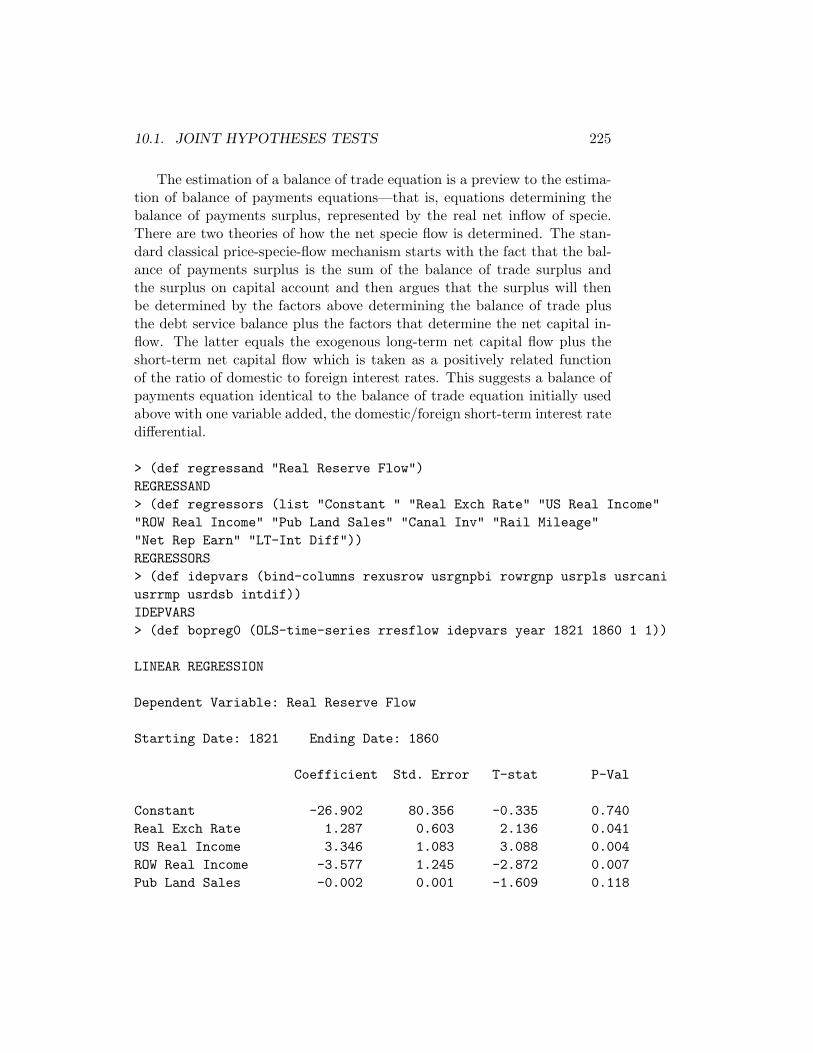
10.1. JOINT HYPOTHESES TESTS 225
The estimation of a balance of trade equation is a preview to the estima-tion of balance of payments equations—that is, equations determining thebalance of payments surplus, represented by the real net inflow of specie.There are two theories of how the net specie flow is determined. The stan-dard classical price-specie-flow mechanism starts with the fact that the bal-ance of payments surplus is the sum of the balance of trade surplus andthe surplus on capital account and then argues that the surplus will thenbe determined by the factors above determining the balance of trade plusthe debt service balance plus the factors that determine the net capital in-flow. The latter equals the exogenous long-term net capital flow plus theshort-term net capital flow which is taken as a positively related functionof the ratio of domestic to foreign interest rates. This suggests a balance ofpayments equation identical to the balance of trade equation initially usedabove with one variable added, the domestic/foreign short-term interest ratedifferential.
> (def regressand "Real Reserve Flow")REGRESSAND> (def regressors (list "Constant " "Real Exch Rate" "US Real Income""ROW Real Income" "Pub Land Sales" "Canal Inv" "Rail Mileage""Net Rep Earn" "LT-Int Diff"))REGRESSORS> (def idepvars (bind-columns rexusrow usrgnpbi rowrgnp usrpls usrcaniusrrmp usrdsb intdif))IDEPVARS> (def bopreg0 (OLS-time-series rresflow idepvars year 1821 1860 1 1))
LINEAR REGRESSION
Dependent Variable: Real Reserve Flow
Starting Date: 1821 Ending Date: 1860
Coefficient Std. Error T-stat P-Val
Constant -26.902 80.356 -0.335 0.740Real Exch Rate 1.287 0.603 2.136 0.041US Real Income 3.346 1.083 3.088 0.004ROW Real Income -3.577 1.245 -2.872 0.007Pub Land Sales -0.002 0.001 -1.609 0.118
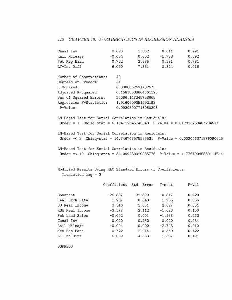
226 CHAPTER 10. FURTHER TOPICS IN REGRESSION ANALYSIS
Canal Inv 0.020 1.862 0.011 0.991Rail Mileage -0.004 0.002 -1.738 0.092Net Rep Earn 0.722 2.575 0.281 0.781LT-Int Diff 6.060 7.351 0.824 0.416
Number of Observations: 40Degrees of Freedom: 31R-Squared: 0.3308652691782573Adjusted R-Squared: 0.15818533864361395Sum of Squared Errors: 25086.147245758668Regression F-Statistic: 1.9160609351292193P-Value: 0.09308907718050308
LM-Based Test for Serial Correlation in Residuals:Order = 1 Chisq-stat = 6.194712545745048 P-Value = 0.012813253407204517
LM-Based Test for Serial Correlation in Residuals:Order =< 3 Chisq-stat = 14.746748575585531 P-Value = 0.002046371879090625
LM-Based Test for Serial Correlation in Residuals:Order =< 10 Chisq-stat = 34.099430920955776 P-Value = 1.77670045580114E-4
Modified Results Using HAC Standard Errors of Coefficients:Truncation lag = 3
Coefficient Std. Error T-stat P-Val
Constant -26.887 32.890 -0.817 0.420Real Exch Rate 1.287 0.648 1.985 0.056US Real Income 3.346 1.651 2.027 0.051ROW Real Income -3.577 2.112 -1.693 0.100Pub Land Sales -0.002 0.001 -1.938 0.062Canal Inv 0.020 0.982 0.020 0.984Rail Mileage -0.004 0.002 -2.743 0.010Net Rep Earn 0.722 2.014 0.359 0.722LT-Int Diff 6.059 4.533 1.337 0.191
BOPREG0
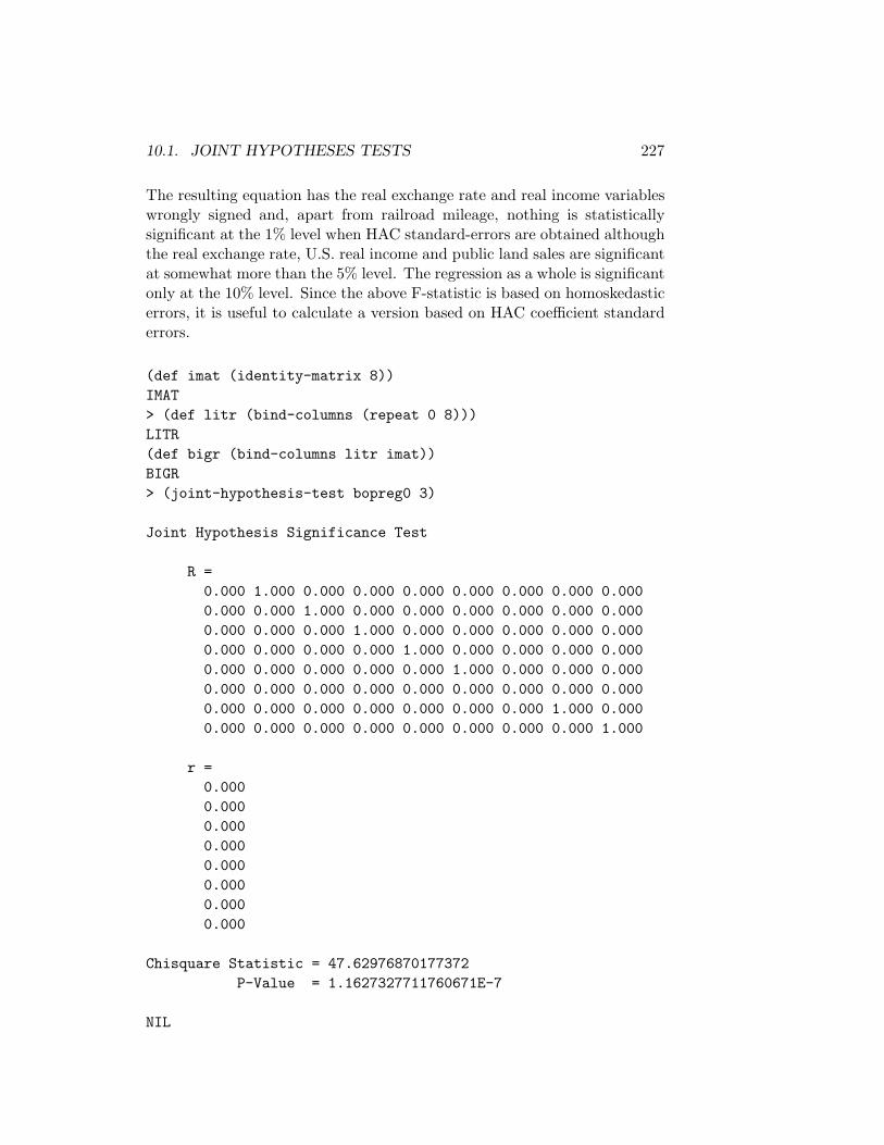
10.1. JOINT HYPOTHESES TESTS 227
The resulting equation has the real exchange rate and real income variableswrongly signed and, apart from railroad mileage, nothing is statisticallysignificant at the 1% level when HAC standard-errors are obtained althoughthe real exchange rate, U.S. real income and public land sales are significantat somewhat more than the 5% level. The regression as a whole is significantonly at the 10% level. Since the above F-statistic is based on homoskedasticerrors, it is useful to calculate a version based on HAC coefficient standarderrors.
(def imat (identity-matrix 8))IMAT> (def litr (bind-columns (repeat 0 8)))LITR(def bigr (bind-columns litr imat))BIGR> (joint-hypothesis-test bopreg0 3)
Joint Hypothesis Significance Test
R =0.000 1.000 0.000 0.000 0.000 0.000 0.000 0.000 0.0000.000 0.000 1.000 0.000 0.000 0.000 0.000 0.000 0.0000.000 0.000 0.000 1.000 0.000 0.000 0.000 0.000 0.0000.000 0.000 0.000 0.000 1.000 0.000 0.000 0.000 0.0000.000 0.000 0.000 0.000 0.000 1.000 0.000 0.000 0.0000.000 0.000 0.000 0.000 0.000 0.000 0.000 0.000 0.0000.000 0.000 0.000 0.000 0.000 0.000 0.000 1.000 0.0000.000 0.000 0.000 0.000 0.000 0.000 0.000 0.000 1.000
r =0.0000.0000.0000.0000.0000.0000.0000.000
Chisquare Statistic = 47.62976870177372P-Value = 1.1627327711760671E-7
NIL

228 CHAPTER 10. FURTHER TOPICS IN REGRESSION ANALYSIS
By this measure the regression as a whole turns out to be statistically sig-nificant but we must keep in mind that this F-test is asymptotically validand we have here only 31 degrees of freedom. Indeed, it is interesting to testthe null-hypothesis that the regression is, in fact, spurious. Phillips-Perrontests on the residuals of the regression yield the following result.
> (def bopresids (send bopreg0 :residuals))BOPRESIDS> (ppunit bopresids "BOP Residuals" 1)
PHILLIPS-PERRON TEST --- BOP ResidualsLags Truncated at 1
Least Squares Estimates:
Constant 1.19076 (3.89816)Trend 0.150196 (0.350802)Lagged Y -0.459965 (0.181064)
R Squared: 0.152049Sigma hat: 24.2283Number of cases: 39Degrees of freedom: 36
Standard t-ratios:
Constant 0.3054661233514375Trend 0.42814886486135173Lagged Y = 0 -2.540347806411093Lagged Y = 1 -8.063263863475918
Least Squares Estimates:
Constant 1.23641 (3.85346)Lagged Y -0.445585 (0.175947)
R Squared: 0.147731Sigma hat: 23.9594Number of cases: 39Degrees of freedom: 37

10.1. JOINT HYPOTHESES TESTS 229
Standard t-ratios:
Constant 0.3208564808157305Lagged Y = 0 -2.5324967921016355Lagged Y = 1 -8.21602611939811
Least Squares Estimates:
Lagged Y -0.440307 (0.173096)
R Squared: 0.145360Sigma hat: 23.6749Number of cases: 39Degrees of freedom: 38
Standard t-ratios:
Lagged Y = 0 -2.5437109552948645Lagged Y = 1 -8.320845831058989
PP t-ratio for Coefficient of Lagged Y = 1:-8.182562762648711
PP t-ratio for Constant = 0:0.27433122076451394
PP t-ratio for Trend Coefficient = 0:0.4842965671890996
PP Statistic for Coefficients of Trend = 0 and Lagged Y = 1:34.05700309671205
PP t-ratio for Coefficient of Lagged Y = 1 in regression without trend:-8.344304386352
PP t-ratio for Coefficient of Lagged Y = 1 in regression withneither constant nor trend:
-8.431710306208258

230 CHAPTER 10. FURTHER TOPICS IN REGRESSION ANALYSIS
> (ppunit bopresids "BOP Residuals" 5)
PHILLIPS-PERRON TEST --- BOP ResidualsLags Truncated at 5
Least Squares Estimates:
Constant 1.19076 (3.89816)Trend 0.150196 (0.350802)Lagged Y -0.459965 (0.181064)
R Squared: 0.152049Sigma hat: 24.2283Number of cases: 39Degrees of freedom: 36
Standard t-ratios:
Constant 0.3054661233514375Trend 0.42814886486135173Lagged Y = 0 -2.540347806411093Lagged Y = 1 -8.063263863475918
Least Squares Estimates:
Constant 1.23641 (3.85346)Lagged Y -0.445585 (0.175947)
R Squared: 0.147731Sigma hat: 23.9594Number of cases: 39Degrees of freedom: 37
Standard t-ratios:
Constant 0.3208564808157305Lagged Y = 0 -2.5324967921016355Lagged Y = 1 -8.21602611939811

10.1. JOINT HYPOTHESES TESTS 231
Least Squares Estimates:
Lagged Y -0.440307 (0.173096)
R Squared: 0.145360Sigma hat: 23.6749Number of cases: 39Degrees of freedom: 38
Standard t-ratios:
Lagged Y = 0 -2.5437109552948645Lagged Y = 1 -8.320845831058989
PP t-ratio for Coefficient of Lagged Y = 1:-9.01676806716786
PP t-ratio for Constant = 0:0.1866501290724194
PP t-ratio for Trend Coefficient = 0:0.6952444241484584
PP Statistic for Coefficients of Trend = 0 and Lagged Y = 1:42.93694292645266
PP t-ratio for Coefficient of Lagged Y = 1 in regression without trend:-9.405545541990548
PP t-ratio for Coefficient of Lagged Y = 1 in regression withneither constant nor trend:
-9.459314068000017
While the number of variables exceeds that covered by the relevant tablein our Statistical Tables, the magnitudes of the statistics obtained suggeststhat the regression is probably not spurious.
The alternative theory of balance of payments adjustment is a portfolio-based theory which takes into account that individuals were free to buy and

232 CHAPTER 10. FURTHER TOPICS IN REGRESSION ANALYSIS
sell assets in exchange for gold across international boundaries. Accordingto this theory, the balance of trade and balance of payments equilibriumshould be unrelated to each other. The real exchange rate adjusts until thebalance of trade equals the net capital outflow. Given the fixed nominalexchange rate, this determines the U.S. price level relative to the price levelabroad. Domestic and foreign residents then buy or sell existing assets inreturn for gold until the world gold stock has been optimally distributedbetween countries. It is changes in the demand or supply of gold alone in acountry that determine its net gold inflow and balance of payments surplus.Accordingly, Trevor Dick and I set up an equation that explains the realreserve flow, or balance of payments surplus, on the basis of changes in thefactors which cause the demand for real money balances to change—namely,the change in domestic real income and domestic interest rates.
Equality of the demand and supply of gold reserves, denoted by G, im-plies that
G = P L(r, Y,m, b) (10.1)
where L(...) is the demand function for gold, P is the general price level (theprice of output in terms of gold), r is the nominal interest rate, Y is thelevel of real income, m is the money multiplier, or the ratio of the quantityof paper money in circulation to the stock of gold, and b is the debt servicebalance which equals interest and dividends received from abroad minusinterest and dividends paid to foreigners. Taking relative changes of thisequation yields
∆G
G=
∆P
P+
∆L(r, Y, m, b)L(r, Y, m, b)
=∆P
P+ η ∆r + ε
∆Y
Y+ µ
∆m
m+ ϑ
∆b
b(10.2)
where η is the interest semi-elasticity of demand for gold, ε is the incomeelasticity of demand for gold, and µ and ϑ are the elasticities of demandfor gold with respect to the money multiplier and the debt service balance.5
Multiplication of both sides by G/P produces
∆G
P=
[G
P
]∆P
P+
[η G
P
]∆r +
[εG
P
]∆Y
Y
+[µG
P
]∆m
m+
[ϑG
P
]∆b
b(10.3)
5I follow a convention here of working with the absolute change rather than the relativechange in the interest rate, which explains why η is the interest semi-elasticity of demandfor gold rather than the actual interest elasticity of demand.
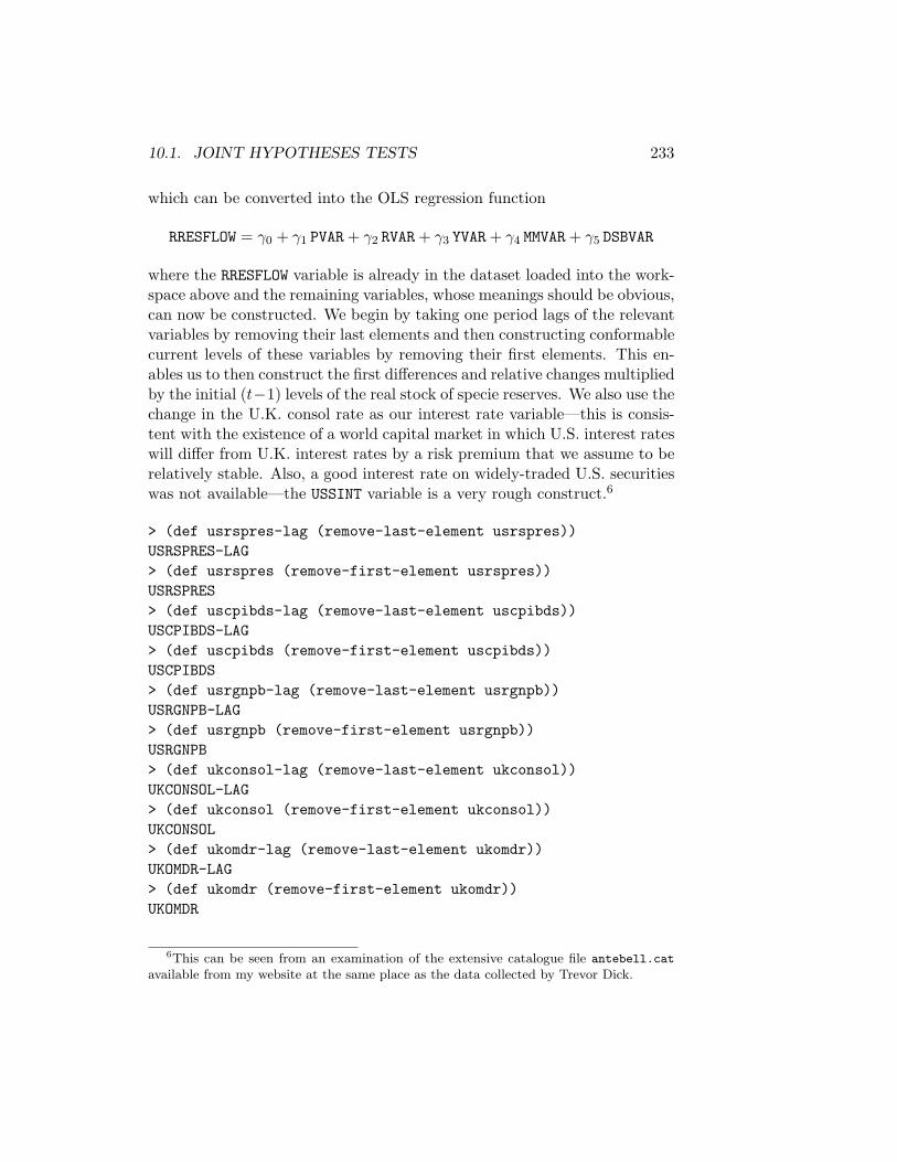
10.1. JOINT HYPOTHESES TESTS 233
which can be converted into the OLS regression function
RRESFLOW = γ0 + γ1 PVAR + γ2 RVAR + γ3 YVAR + γ4 MMVAR + γ5 DSBVAR
where the RRESFLOW variable is already in the dataset loaded into the work-space above and the remaining variables, whose meanings should be obvious,can now be constructed. We begin by taking one period lags of the relevantvariables by removing their last elements and then constructing conformablecurrent levels of these variables by removing their first elements. This en-ables us to then construct the first differences and relative changes multipliedby the initial (t−1) levels of the real stock of specie reserves. We also use thechange in the U.K. consol rate as our interest rate variable—this is consis-tent with the existence of a world capital market in which U.S. interest rateswill differ from U.K. interest rates by a risk premium that we assume to berelatively stable. Also, a good interest rate on widely-traded U.S. securitieswas not available—the USSINT variable is a very rough construct.6
> (def usrspres-lag (remove-last-element usrspres))USRSPRES-LAG> (def usrspres (remove-first-element usrspres))USRSPRES> (def uscpibds-lag (remove-last-element uscpibds))USCPIBDS-LAG> (def uscpibds (remove-first-element uscpibds))USCPIBDS> (def usrgnpb-lag (remove-last-element usrgnpb))USRGNPB-LAG> (def usrgnpb (remove-first-element usrgnpb))USRGNPB> (def ukconsol-lag (remove-last-element ukconsol))UKCONSOL-LAG> (def ukconsol (remove-first-element ukconsol))UKCONSOL> (def ukomdr-lag (remove-last-element ukomdr))UKOMDR-LAG> (def ukomdr (remove-first-element ukomdr))UKOMDR
6This can be seen from an examination of the extensive catalogue file antebell.cat
available from my website at the same place as the data collected by Trevor Dick.
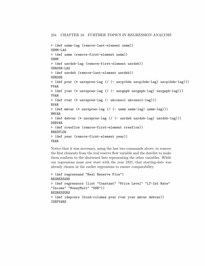
234 CHAPTER 10. FURTHER TOPICS IN REGRESSION ANALYSIS
> (def usmm-lag (remove-last-element usmm))USMM-LAG> (def usmm (remove-first-element usmm))USMM> (def usrdsb-lag (remove-first-element usrdsb))USRDSB-LAG> (def usrdsb (remove-last-element usrdsb))USRDSB> (def pvar (* usrspres-lag (/ (- uscpibds uscpibds-lag) uscpibds-lag)))PVAR> (def yvar (* usrspres-lag (/ (- usrgnpb usrgnpb-lag) usrgnpb-lag)))YVAR> (def rvar (* usrspres-lag (- ukconsol ukconsol-lag)))RVAR> (def mmvar (* usrspres-lag (/ (- usmm usmm-lag) usmm-lag)))MMVAR> (def dsbvar (* usrspres-lag (/ (- usrdsb usrdsb-lag) usrdsb-lag)))DSBVAR> (def rresflow (remove-first-element rresflow))RRESFLOW> (def year (remove-first-element year))YEAR
Notice that it was necessary, using the last two commands above, to removethe first elements from the real reserve flow variable and the datelist to makethem conform to the shortened lists representing the other variables. Whileour regressions must now start with the year 1821, that starting-date wasalready chosen in the earlier regressions to ensure comparability.
> (def regressand "Real Reserve Flow")REGRESSAND> (def regressors (list "Constant" "Price Level" "LT-Int Rate""Income" "MoneyMult" "DSB"))REGRESSORS> (def idepvars (bind-columns pvar rvar yvar mmvar dsbvar))IDEPVARS
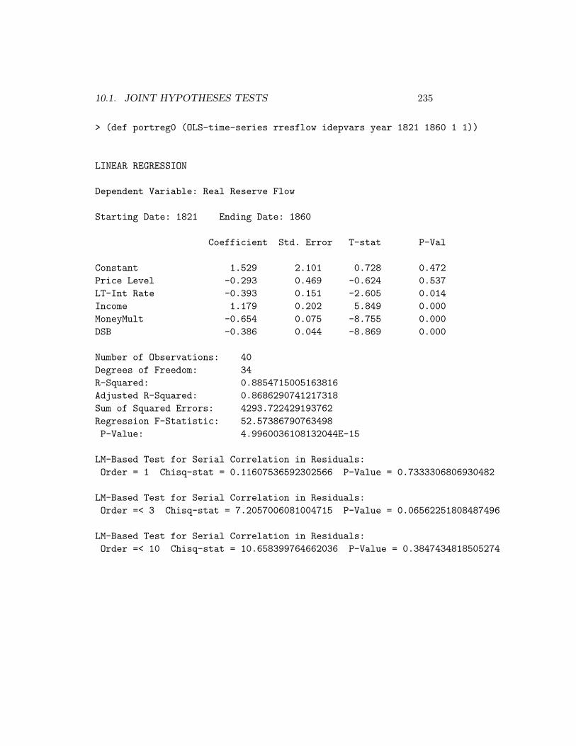
10.1. JOINT HYPOTHESES TESTS 235
> (def portreg0 (OLS-time-series rresflow idepvars year 1821 1860 1 1))
LINEAR REGRESSION
Dependent Variable: Real Reserve Flow
Starting Date: 1821 Ending Date: 1860
Coefficient Std. Error T-stat P-Val
Constant 1.529 2.101 0.728 0.472Price Level -0.293 0.469 -0.624 0.537LT-Int Rate -0.393 0.151 -2.605 0.014Income 1.179 0.202 5.849 0.000MoneyMult -0.654 0.075 -8.755 0.000DSB -0.386 0.044 -8.869 0.000
Number of Observations: 40Degrees of Freedom: 34R-Squared: 0.8854715005163816Adjusted R-Squared: 0.8686290741217318Sum of Squared Errors: 4293.722429193762Regression F-Statistic: 52.57386790763498P-Value: 4.9960036108132044E-15
LM-Based Test for Serial Correlation in Residuals:Order = 1 Chisq-stat = 0.11607536592302566 P-Value = 0.7333306806930482
LM-Based Test for Serial Correlation in Residuals:Order =< 3 Chisq-stat = 7.2057006081004715 P-Value = 0.06562251808487496
LM-Based Test for Serial Correlation in Residuals:Order =< 10 Chisq-stat = 10.658399764662036 P-Value = 0.3847434818505274

236 CHAPTER 10. FURTHER TOPICS IN REGRESSION ANALYSIS
Modified Results Using HAC Standard Errors of Coefficients:Truncation lag = 3
Coefficient Std. Error T-stat P-Val
Constant 1.529 1.681 0.910 0.369Price Level -0.293 0.362 -0.809 0.424LT-Int Rate -0.393 0.167 -2.349 0.025Income 1.179 0.173 6.797 0.000MoneyMult -0.654 0.047 -13.878 0.000DSB -0.386 0.016 -23.417 0.000
PORTREG0
Since serial correlation in the residuals was found for less than three lags atthe 10% level and not at all for less than 10 lags, we should pay attentiononly to the results with non-HAC coefficient standard errors. Contrary towhat would have been expected, the price variable is not only less than unitybut also negative. Upon reflection, it would appear that this is due to thefact that our price variable represents the level of current inflation which notonly increases the quantity of specie that would have to be held to keep thereal stock of specie constant, but also increases the alternative opportunitycost of holding specie—this cost would be incorporated in a U.S. interest ratevariable but not in the U.K. consol rate. The relative change in the debtservice balance was included because Trevor and I found it to be significantin similar Canadian and Australian regressions.7 I suspect that this variable,which is negative and increases in size over the period, captures the increasein the demand for specie reserves associated with the development of theU.S. economy over the period—it is really a proxy for the net capital inflowwhich increased over the period. Since that imported capital was ownedabroad, it’s return did not form part of U.S. GNP but its growth increasedthe volume of transactions that had to be made in the U.S. economy. Incomparison to the classical specie-flow regression, the results here indicate ahigh degree of statistical significance of all but the price level variable with
7See Trevor J. O. Dick and John E. Floyd, Canada and the Gold Standard, CambridgeUniversity Press, 1992, and T. J. O. Dick, John E. Floyd and David Pope, “Balance ofPayments Adjustment Under Gold Standard Policies: Canada and Australia Compared,”in T. Bayoumi, B. Eichengreen and M. Taylor, eds. Modern Perspectives on the GoldStandard, Cambridge University Press, 1996.
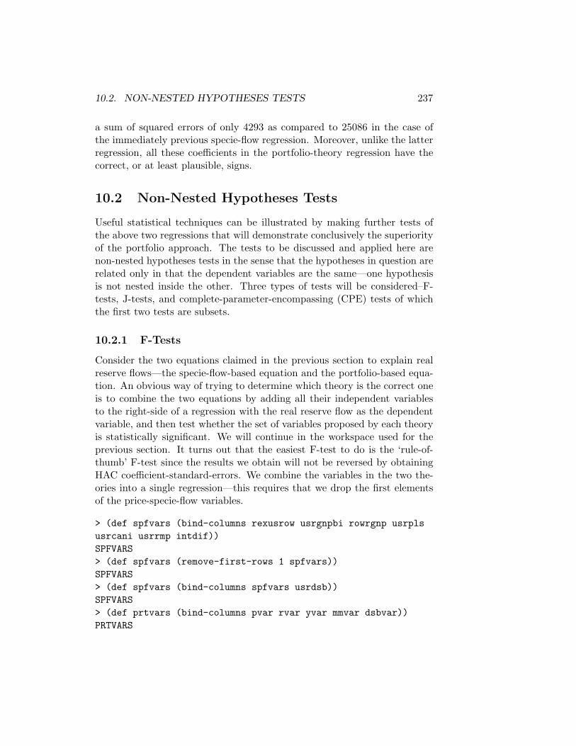
10.2. NON-NESTED HYPOTHESES TESTS 237
a sum of squared errors of only 4293 as compared to 25086 in the case ofthe immediately previous specie-flow regression. Moreover, unlike the latterregression, all these coefficients in the portfolio-theory regression have thecorrect, or at least plausible, signs.
10.2 Non-Nested Hypotheses Tests
Useful statistical techniques can be illustrated by making further tests ofthe above two regressions that will demonstrate conclusively the superiorityof the portfolio approach. The tests to be discussed and applied here arenon-nested hypotheses tests in the sense that the hypotheses in question arerelated only in that the dependent variables are the same—one hypothesisis not nested inside the other. Three types of tests will be considered–F-tests, J-tests, and complete-parameter-encompassing (CPE) tests of whichthe first two tests are subsets.
10.2.1 F-Tests
Consider the two equations claimed in the previous section to explain realreserve flows—the specie-flow-based equation and the portfolio-based equa-tion. An obvious way of trying to determine which theory is the correct oneis to combine the two equations by adding all their independent variablesto the right-side of a regression with the real reserve flow as the dependentvariable, and then test whether the set of variables proposed by each theoryis statistically significant. We will continue in the workspace used for theprevious section. It turns out that the easiest F-test to do is the ‘rule-of-thumb’ F-test since the results we obtain will not be reversed by obtainingHAC coefficient-standard-errors. We combine the variables in the two the-ories into a single regression—this requires that we drop the first elementsof the price-specie-flow variables.
> (def spfvars (bind-columns rexusrow usrgnpbi rowrgnp usrplsusrcani usrrmp intdif))SPFVARS> (def spfvars (remove-first-rows 1 spfvars))SPFVARS> (def spfvars (bind-columns spfvars usrdsb))SPFVARS> (def prtvars (bind-columns pvar rvar yvar mmvar dsbvar))PRTVARS
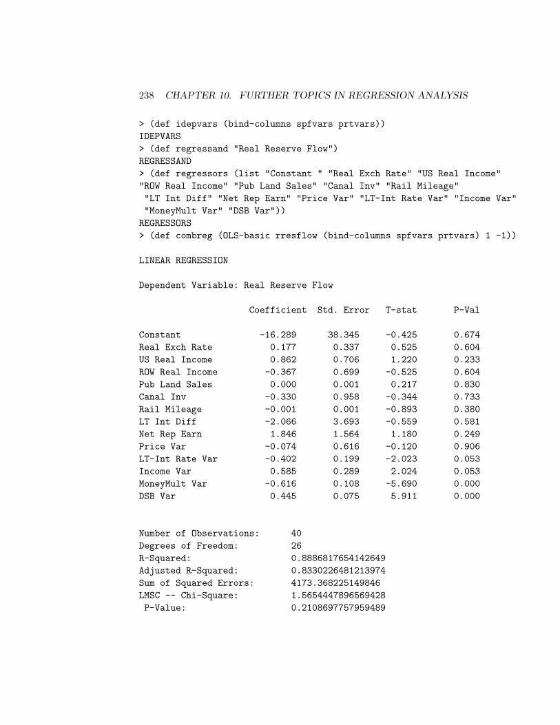
238 CHAPTER 10. FURTHER TOPICS IN REGRESSION ANALYSIS
> (def idepvars (bind-columns spfvars prtvars))IDEPVARS> (def regressand "Real Reserve Flow")REGRESSAND> (def regressors (list "Constant " "Real Exch Rate" "US Real Income""ROW Real Income" "Pub Land Sales" "Canal Inv" "Rail Mileage""LT Int Diff" "Net Rep Earn" "Price Var" "LT-Int Rate Var" "Income Var""MoneyMult Var" "DSB Var"))REGRESSORS> (def combreg (OLS-basic rresflow (bind-columns spfvars prtvars) 1 -1))
LINEAR REGRESSION
Dependent Variable: Real Reserve Flow
Coefficient Std. Error T-stat P-Val
Constant -16.289 38.345 -0.425 0.674Real Exch Rate 0.177 0.337 0.525 0.604US Real Income 0.862 0.706 1.220 0.233ROW Real Income -0.367 0.699 -0.525 0.604Pub Land Sales 0.000 0.001 0.217 0.830Canal Inv -0.330 0.958 -0.344 0.733Rail Mileage -0.001 0.001 -0.893 0.380LT Int Diff -2.066 3.693 -0.559 0.581Net Rep Earn 1.846 1.564 1.180 0.249Price Var -0.074 0.616 -0.120 0.906LT-Int Rate Var -0.402 0.199 -2.023 0.053Income Var 0.585 0.289 2.024 0.053MoneyMult Var -0.616 0.108 -5.690 0.000DSB Var 0.445 0.075 5.911 0.000
Number of Observations: 40Degrees of Freedom: 26R-Squared: 0.8886817654142649Adjusted R-Squared: 0.8330226481213974Sum of Squared Errors: 4173.368225149846LMSC -- Chi-Square: 1.5654447896569428P-Value: 0.2108697757959489
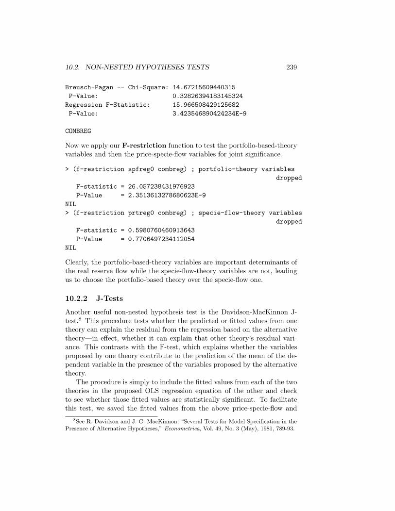
10.2. NON-NESTED HYPOTHESES TESTS 239
Breusch-Pagan -- Chi-Square: 14.67215609440315P-Value: 0.32826394183145324
Regression F-Statistic: 15.966508429125682P-Value: 3.423546890424234E-9
COMBREG
Now we apply our F-restriction function to test the portfolio-based-theoryvariables and then the price-specie-flow variables for joint significance.
> (f-restriction spfreg0 combreg) ; portfolio-theory variablesdropped
F-statistic = 26.057238431976923P-Value = 2.3513613278680623E-9
NIL> (f-restriction prtreg0 combreg) ; specie-flow-theory variables
droppedF-statistic = 0.5980760460913643P-Value = 0.7706497234112054
NIL
Clearly, the portfolio-based-theory variables are important determinants ofthe real reserve flow while the specie-flow-theory variables are not, leadingus to choose the portfolio-based theory over the specie-flow one.
10.2.2 J-Tests
Another useful non-nested hypothesis test is the Davidson-MacKinnon J-test.8 This procedure tests whether the predicted or fitted values from onetheory can explain the residual from the regression based on the alternativetheory—in effect, whether it can explain that other theory’s residual vari-ance. This contrasts with the F-test, which explains whether the variablesproposed by one theory contribute to the prediction of the mean of the de-pendent variable in the presence of the variables proposed by the alternativetheory.
The procedure is simply to include the fitted values from each of the twotheories in the proposed OLS regression equation of the other and checkto see whether those fitted values are statistically significant. To facilitatethis test, we saved the fitted values from the above price-specie-flow and
8See R. Davidson and J. G. MacKinnon, “Several Tests for Model Specification in thePresence of Alternative Hypotheses,” Econometrica, Vol. 49, No. 3 (May), 1981, 789-93.
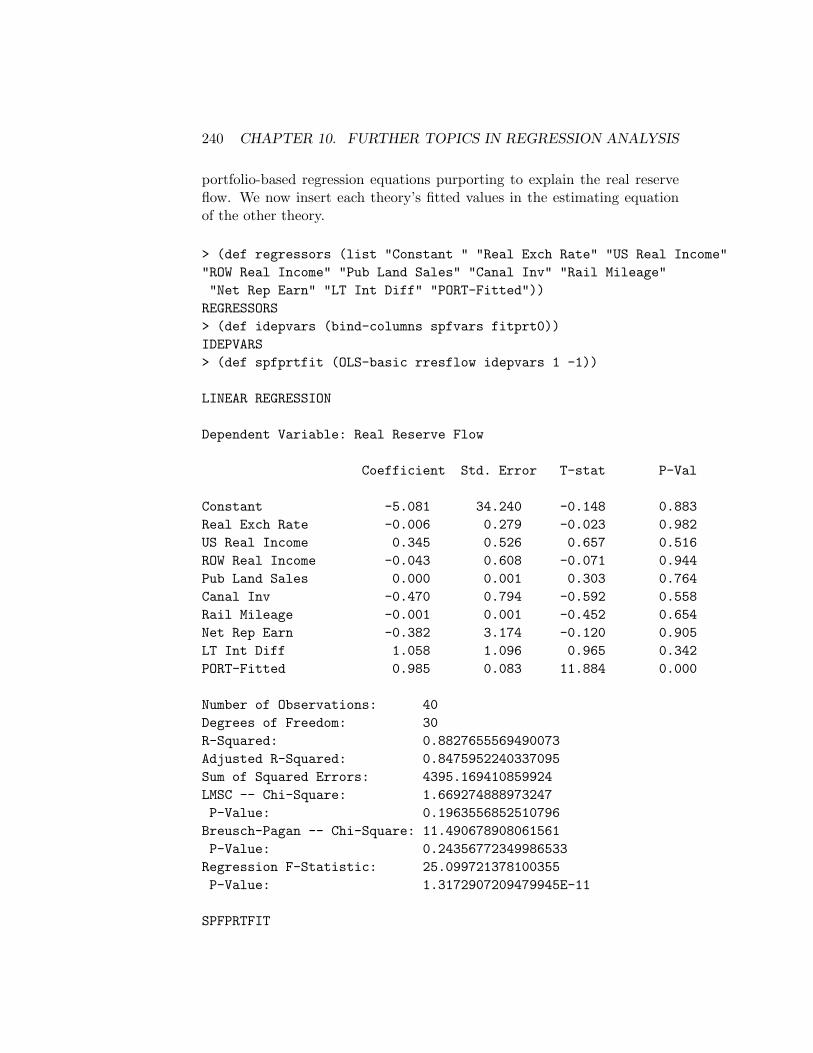
240 CHAPTER 10. FURTHER TOPICS IN REGRESSION ANALYSIS
portfolio-based regression equations purporting to explain the real reserveflow. We now insert each theory’s fitted values in the estimating equationof the other theory.
> (def regressors (list "Constant " "Real Exch Rate" "US Real Income""ROW Real Income" "Pub Land Sales" "Canal Inv" "Rail Mileage""Net Rep Earn" "LT Int Diff" "PORT-Fitted"))REGRESSORS> (def idepvars (bind-columns spfvars fitprt0))IDEPVARS> (def spfprtfit (OLS-basic rresflow idepvars 1 -1))
LINEAR REGRESSION
Dependent Variable: Real Reserve Flow
Coefficient Std. Error T-stat P-Val
Constant -5.081 34.240 -0.148 0.883Real Exch Rate -0.006 0.279 -0.023 0.982US Real Income 0.345 0.526 0.657 0.516ROW Real Income -0.043 0.608 -0.071 0.944Pub Land Sales 0.000 0.001 0.303 0.764Canal Inv -0.470 0.794 -0.592 0.558Rail Mileage -0.001 0.001 -0.452 0.654Net Rep Earn -0.382 3.174 -0.120 0.905LT Int Diff 1.058 1.096 0.965 0.342PORT-Fitted 0.985 0.083 11.884 0.000
Number of Observations: 40Degrees of Freedom: 30R-Squared: 0.8827655569490073Adjusted R-Squared: 0.8475952240337095Sum of Squared Errors: 4395.169410859924LMSC -- Chi-Square: 1.669274888973247P-Value: 0.1963556852510796Breusch-Pagan -- Chi-Square: 11.490678908061561P-Value: 0.24356772349986533Regression F-Statistic: 25.099721378100355P-Value: 1.3172907209479945E-11
SPFPRTFIT
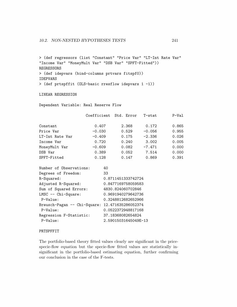
10.2. NON-NESTED HYPOTHESES TESTS 241
> (def regressors (list "Constant" "Price Var" "LT-Int Rate Var""Income Var" "MoneyMult Var" "DSB Var" "SPFT-Fitted"))REGRESSORS> (def idepvars (bind-columns prtvars fitspf0))IDEPVARS> (def prtspffit (OLS-basic rresflow idepvars 1 -1))
LINEAR REGRESSION
Dependent Variable: Real Reserve Flow
Coefficient Std. Error T-stat P-Val
Constant 0.407 2.368 0.172 0.865Price Var -0.030 0.529 -0.056 0.955LT-Int Rate Var -0.409 0.175 -2.336 0.026Income Var 0.720 0.240 3.002 0.005MoneyMult Var -0.609 0.082 -7.471 0.000DSB Var 0.389 0.052 7.514 0.000SPFT-Fitted 0.128 0.147 0.869 0.391
Number of Observations: 40Degrees of Freedom: 33R-Squared: 0.8711451333742724Adjusted R-Squared: 0.8477169758059583Sum of Squared Errors: 4830.824060702846LMSC -- Chi-Square: 0.9691940279642736P-Value: 0.3248812682652966
Breusch-Pagan -- Chi-Square: 12.471635286052374P-Value: 0.0522372948817168
Regression F-Statistic: 37.18368082654824P-Value: 2.59015031645049E-13
PRTSPFFIT
The portfolio-based theory fitted values clearly are significant in the price-specie-flow equation but the specie-flow fitted values are statistically in-significant in the portfolio-based estimating equation, further confirmingour conclusion in the case of the F-tests.
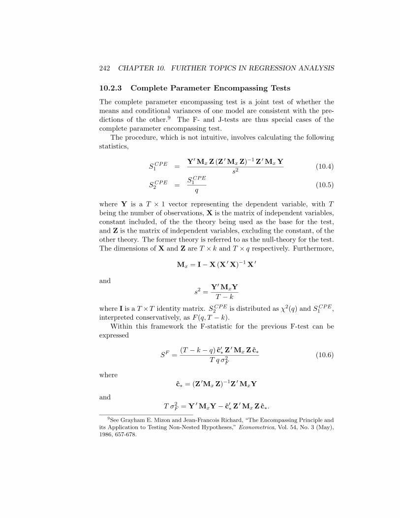
242 CHAPTER 10. FURTHER TOPICS IN REGRESSION ANALYSIS
10.2.3 Complete Parameter Encompassing Tests
The complete parameter encompassing test is a joint test of whether themeans and conditional variances of one model are consistent with the pre-dictions of the other.9 The F- and J-tests are thus special cases of thecomplete parameter encompassing test.
The procedure, which is not intuitive, involves calculating the followingstatistics,
S CPE1 =
Y′Mx Z (Z ′Mx Z)−1 Z ′Mx Ys2
(10.4)
S CPE2 =
S CPE1
q(10.5)
where Y is a T × 1 vector representing the dependent variable, with Tbeing the number of observations, X is the matrix of independent variables,constant included, of the the theory being used as the base for the test,and Z is the matrix of independent variables, excluding the constant, of theother theory. The former theory is referred to as the null-theory for the test.The dimensions of X and Z are T × k and T × q respectively. Furthermore,
Mx = I−X (X ′X)−1 X ′
and
s2 =Y′MxYT − k
where I is a T ×T identity matrix. S CPE2 is distributed as χ2(q) and S CPE
1 ,interpreted conservatively, as F (q, T − k).
Within this framework the F-statistic for the previous F-test can beexpressed
SF =(T − k − q) c′∗ Z ′Mx Z c∗
T q σ2F
(10.6)
wherec∗ = (Z ′Mx Z)−1Z ′MxY
andT σ2
F = Y ′MxY − c′∗ Z′Mx Z c∗.
9See Grayham E. Mizon and Jean-Francois Richard, “The Encompassing Principle andits Application to Testing Non-Nested Hypotheses,” Econometrica, Vol. 54, No. 3 (May),1986, 657-678.

10.2. NON-NESTED HYPOTHESES TESTS 243
This F-statistic has q degrees of freedom in the numerator and T − k − qdegrees of freedom in the denominator. After we add a constant term to thematrix Z, the F-statistic for the J-test is
SJ =(T − k − 1) u2 γ ′ Z ′Mx Z γ
T σ2J
(10.7)
whereγ = (Z ′ Z)−1Z ′Y
u = (γ ′ Z ′Mx Z γ)−1 γ ′ Z ′MxY
andT σ2
J = Y ′MxY − u2 γ ′ Z ′Mx Z γ.
This F-statistic has q degrees of freedom in the numerator and T −k degreesof freedom in the denominator.
I have written the function CPE-test to perform the above calculations.The function takes four arguments—in order, the dependent variable list,the matrix of independent variables for the null-theory and the matrix ofindependent variables for the alternative theory, excluding the constant inboth cases and, finally, a string expression giving an appropriate name forthe null-theory. We now apply this function in the XLispStat workspaceabove.
> (CPE-test rresflow spfvars prtvars "Price-Specie-Flow Theory")
COMPLETE PARAMETER ENCOMPASSING TEST OF REGRESSORS
Null theory (null-hypothesis --> no effects of other theory):
===> Price-Specie-Flow Theory
F-test F-statistic = 26.057238431977044P-Value = 2.3513613278680623E-9
J-test F-statistic = 141.22989969697537P-Value = 0.0
CPE Chisq-statistic = 25.84279456258403P-Value = 9.572338076979658E-5
CPE F-statistic = 5.168558912516806P-Value = 0.0014580336808481809
NIL
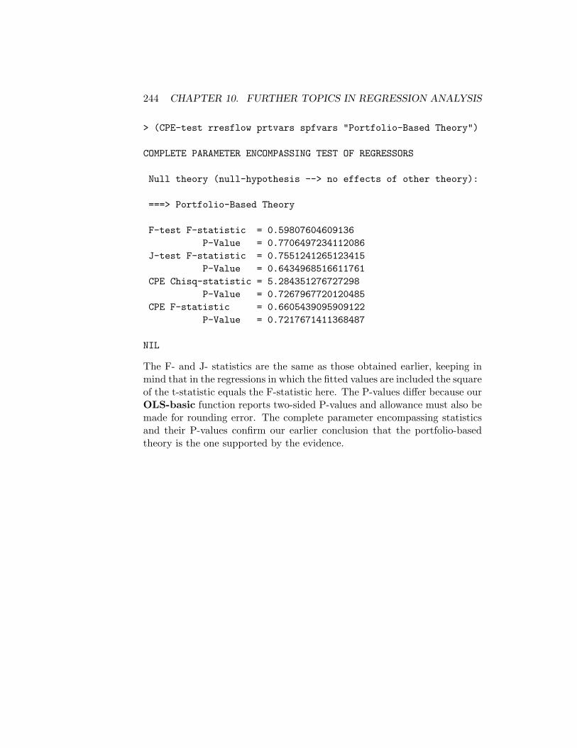
244 CHAPTER 10. FURTHER TOPICS IN REGRESSION ANALYSIS
> (CPE-test rresflow prtvars spfvars "Portfolio-Based Theory")
COMPLETE PARAMETER ENCOMPASSING TEST OF REGRESSORS
Null theory (null-hypothesis --> no effects of other theory):
===> Portfolio-Based Theory
F-test F-statistic = 0.59807604609136P-Value = 0.7706497234112086
J-test F-statistic = 0.7551241265123415P-Value = 0.6434968516611761
CPE Chisq-statistic = 5.284351276727298P-Value = 0.7267967720120485
CPE F-statistic = 0.6605439095909122P-Value = 0.7217671411368487
NIL
The F- and J- statistics are the same as those obtained earlier, keeping inmind that in the regressions in which the fitted values are included the squareof the t-statistic equals the F-statistic here. The P-values differ because ourOLS-basic function reports two-sided P-values and allowance must also bemade for rounding error. The complete parameter encompassing statisticsand their P-values confirm our earlier conclusion that the portfolio-basedtheory is the one supported by the evidence.

10.3. GENERALISED LEAST SQUARES 245
10.3 Generalised Least Squares
As demonstrated by the many regression results above, heteroskedasticityand autocorrelation in the residuals is a widespread problem. One way ofdealing with it is to calculate HAC coefficient standard errors. Another wayis using generalised least squares instead of standard OLS.
10.3.1 The Nature of GLS
The basic assumption of ordinary least squares analysis is that the residualshave constant variance and are uncorrelated. This implies that the variancecovariance matrix of the residuals will equal σ2I, where I is a T ×T identitymatrix with T being the number of observations. The estimated coefficientsare given by
b = (X′X)−1
= (X′ (σ2 I)−1 X)−1 X′ (σ2 I)−1 Y (10.8)
and the variance-covariance matrix of the coefficients is equal to
V = σ2 (X′X)−1 = (X′ (σ2 I)−1 X)−1. (10.9)
When the residuals are heteroskedastic, σ2 I is replaced by a matrix Ω whichhas unequal diagonal elements with off-diagonal elements equal to zero. Andwhen the residuals are autocorrelated, at least some of the off-diagonal ele-ments of Ω will be non-zero. When we have an estimate of this symmetricmatrix, call it Ω, the above two estimating equations become
b = (X′ Ω−1 X)−1 X′ Ω−1 Y (10.10)V = (X′ Ω−1 X)−1. (10.11)
An example in the case of heteroskedasticity alone is a situation wherethe σ2
i happen to be proportional to the square of a variable zi, (i = 1....T ),which may or may not actually be an independent variable in the regression.In this case,
Ω =
σ2z21 0 0 · · · · · · 0
0 σ2z22 0 · · · · · · 0
0 0 σ2z23 · · · · · · 0
· · · · · · · · · · · · · · · 0· · · · · · · · · · · · · · · 00 0 0 0 0 σ2z2
T
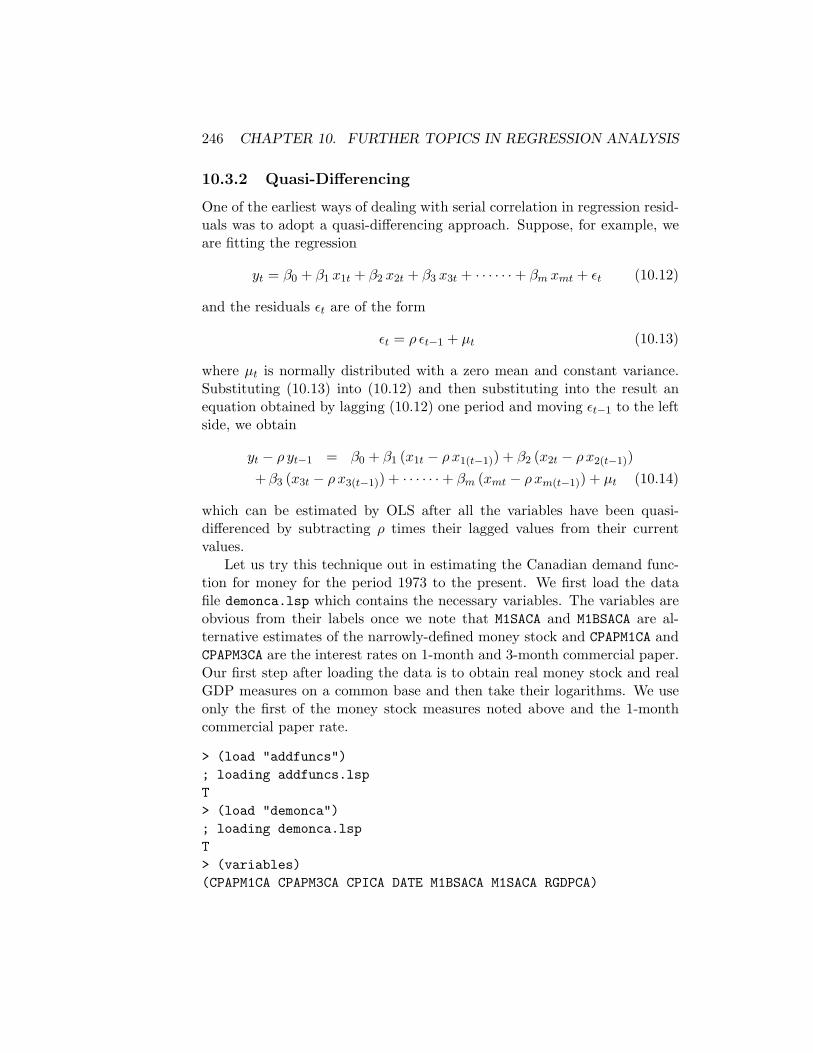
246 CHAPTER 10. FURTHER TOPICS IN REGRESSION ANALYSIS
10.3.2 Quasi-Differencing
One of the earliest ways of dealing with serial correlation in regression resid-uals was to adopt a quasi-differencing approach. Suppose, for example, weare fitting the regression
yt = β0 + β1 x1t + β2 x2t + β3 x3t + · · · · · ·+ βm xmt + εt (10.12)
and the residuals εt are of the form
εt = ρ εt−1 + µt (10.13)
where µt is normally distributed with a zero mean and constant variance.Substituting (10.13) into (10.12) and then substituting into the result anequation obtained by lagging (10.12) one period and moving εt−1 to the leftside, we obtain
yt − ρ yt−1 = β0 + β1 (x1t − ρ x1(t−1)) + β2 (x2t − ρ x2(t−1))+β3 (x3t − ρ x3(t−1)) + · · · · · ·+ βm (xmt − ρ xm(t−1)) + µt (10.14)
which can be estimated by OLS after all the variables have been quasi-differenced by subtracting ρ times their lagged values from their currentvalues.
Let us try this technique out in estimating the Canadian demand func-tion for money for the period 1973 to the present. We first load the datafile demonca.lsp which contains the necessary variables. The variables areobvious from their labels once we note that M1SACA and M1BSACA are al-ternative estimates of the narrowly-defined money stock and CPAPM1CA andCPAPM3CA are the interest rates on 1-month and 3-month commercial paper.Our first step after loading the data is to obtain real money stock and realGDP measures on a common base and then take their logarithms. We useonly the first of the money stock measures noted above and the 1-monthcommercial paper rate.
> (load "addfuncs"); loading addfuncs.lspT> (load "demonca"); loading demonca.lspT> (variables)(CPAPM1CA CPAPM3CA CPICA DATE M1BSACA M1SACA RGDPCA)
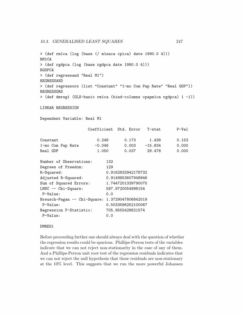
10.3. GENERALISED LEAST SQUARES 247
> (def rm1ca (log (base (/ m1saca cpica) date 1990.0 4)))RM1CA> (def rgdpca (log (base rgdpca date 1990.0 4)))RGDPCA> (def regressand "Real M1")REGRESSAND> (def regressors (list "Constant" "1-mo Com Pap Rate" "Real GDP"))REGRESSORS> (def dmreg1 (OLS-basic rm1ca (bind-columns cpapm1ca rgdpca) 1 -1))
LINEAR REGRESSION
Dependent Variable: Real M1
Coefficient Std. Error T-stat P-Val
Constant 0.248 0.173 1.438 0.1531-mo Com Pap Rate -0.046 0.003 -15.834 0.000Real GDP 1.050 0.037 28.478 0.000
Number of Observations: 132Degrees of Freedom: 129R-Squared: 0.9162832942178732Adjusted R-Squared: 0.9149853607948946Sum of Squared Errors: 1.7447201339790075LMSC -- Chi-Square: 597.9720054998154P-Value: 0.0
Breusch-Pagan -- Chi-Square: 1.3729047806842019P-Value: 0.5033586252100067
Regression F-Statistic: 705.9555428621574P-Value: 0.0
DMREG1
Before proceeding further one should always deal with the question of whetherthe regression results could be spurious. Phillips-Perron tests of the variablesindicate that we can not reject non-stationarity in the case of any of them.And a Phillips-Perron unit root test of the regression residuals indicates thatwe can not reject the null hypothesis that these residuals are non-stationaryat the 10% level. This suggests that we run the more powerful Johansen
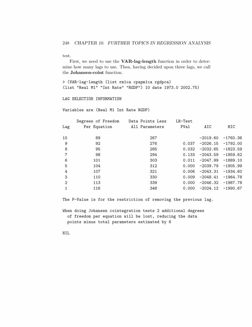
248 CHAPTER 10. FURTHER TOPICS IN REGRESSION ANALYSIS
test.First, we need to use the VAR-lag-length function in order to deter-
mine how many lags to use. Then, having decided upon three lags, we callthe Johansen-coint function.
> (VAR-lag-length (list rm1ca cpapm1ca rgdpca)(list "Real M1" "Int Rate" "RGDP") 10 date 1973.0 2002.75)
LAG SELECTION INFORMATION
Variables are (Real M1 Int Rate RGDP)
Degrees of Freedom Data Points Less LR-TestLag Per Equation All Parameters PVal AIC BIC
10 89 267 -2019.60 -1760.369 92 276 0.037 -2026.15 -1792.008 95 285 0.032 -2032.65 -1823.597 98 294 0.133 -2043.59 -1859.626 101 303 0.011 -2047.99 -1889.105 104 312 0.000 -2039.79 -1905.994 107 321 0.006 -2043.31 -1934.603 110 330 0.009 -2048.41 -1964.782 113 339 0.000 -2046.32 -1987.781 116 348 0.000 -2024.12 -1990.67
The P-Value is for the restriction of removing the previous lag.
When doing Johansen cointegration tests 2 additional degreesof freedom per equation will be lost, reducing the datapoints minus total parameters estimated by 6
NIL

10.3. GENERALISED LEAST SQUARES 249
> (Johansen-coint (list rm1ca cpapm1ca rgdpca)(list "Real M1" "IntRate" "RGDP") 1 date 1973.0 2002.75 1)
JOHANSEN COINTEGRATION TEST
Variables are (Real M1 IntRate RGDP)
Number of Lags = 3
Results when deterministic trends are included:
CointVectors Eigen-
Under Null Values L-max Trace
0.000 0.159 20.791 34.7301.000 0.110 13.921 13.9392.000 0.000 0.018 0.018
Eigenvectors together with the associated variables
Real M1 -1.000 -1.000IntRate -0.117 -0.044RGDP 0.215 1.504
Exclusion tests of variables in the cointegrating relationships
Real M1 0.153 0.001IntRate 0.023 0.000RGDP 0.805 0.000
Likelihood Ratio Tests of null hypothesis of no deterministic trendsbut constants in the cointegrating vectors against the alternativeof no restrictions on deterministic trends
Coint ChisqVectors P-Values
1.000 0.0072.000 0.004

250 CHAPTER 10. FURTHER TOPICS IN REGRESSION ANALYSIS
Results when deterministic trends are not included and con-stants are present in the cointegrating relationships:
CointVectors Eigen-Under Null Values L-max Trace
0.000 0.210 28.350 52.2661.000 0.123 15.784 23.9152.000 0.066 8.131 8.131
Eigenvectors together with the associated variables
Real M1 -1.000 -1.000constant 10.984 0.160IntRate -0.180 -0.066RGDP -0.857 1.111
Exclusion tests of variables in the cointegrating relationships
constant 0.001 0.595Real M1 0.449 0.007IntRate 0.062 0.006RGDP 0.582 0.018
Likelihood Ratio Tests of null hypothesis of no deterministictrends and no constants in the cointegrating relationshipsversus the alternative of no deterministic trends withconstants in the cointegrating relationships
Coint ChisqVectors P-Values
1.000 0.0002.000 0.000
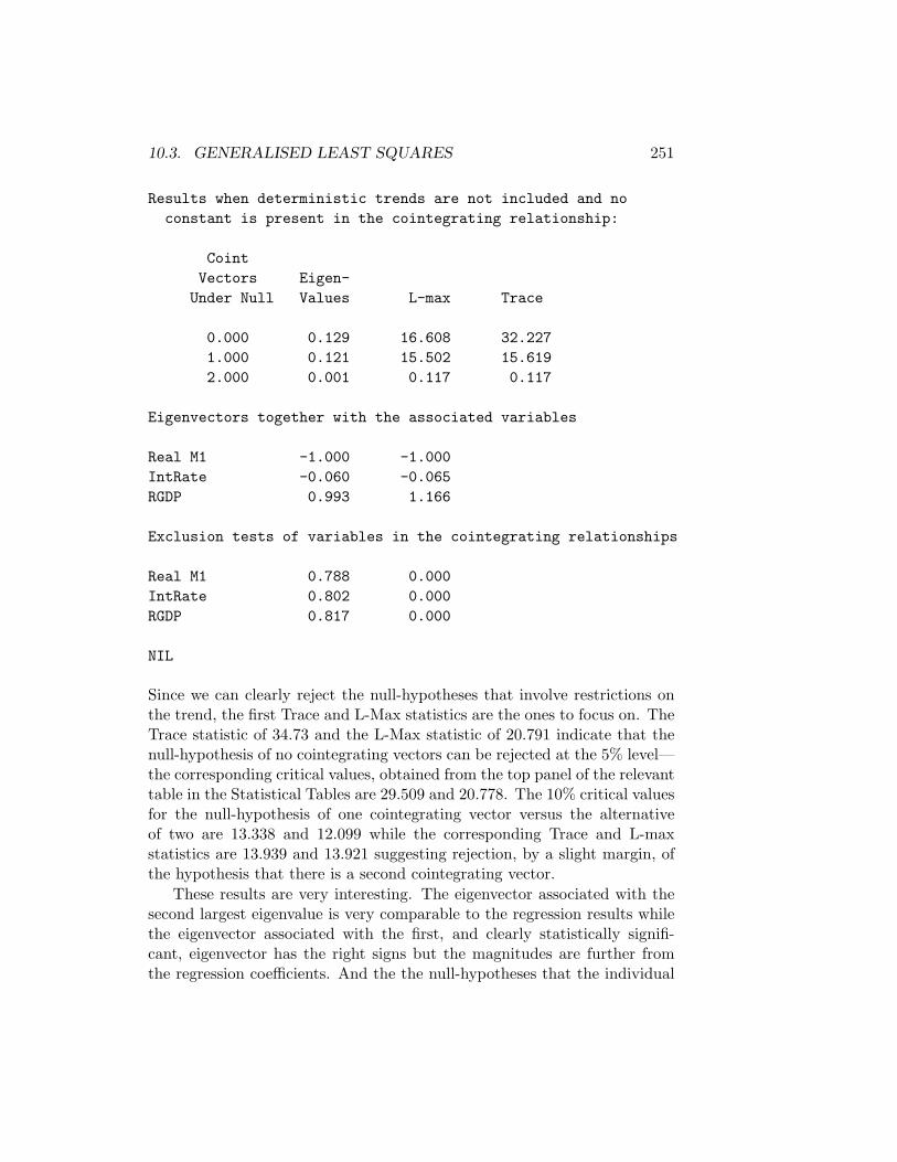
10.3. GENERALISED LEAST SQUARES 251
Results when deterministic trends are not included and noconstant is present in the cointegrating relationship:
CointVectors Eigen-
Under Null Values L-max Trace
0.000 0.129 16.608 32.2271.000 0.121 15.502 15.6192.000 0.001 0.117 0.117
Eigenvectors together with the associated variables
Real M1 -1.000 -1.000IntRate -0.060 -0.065RGDP 0.993 1.166
Exclusion tests of variables in the cointegrating relationships
Real M1 0.788 0.000IntRate 0.802 0.000RGDP 0.817 0.000
NIL
Since we can clearly reject the null-hypotheses that involve restrictions onthe trend, the first Trace and L-Max statistics are the ones to focus on. TheTrace statistic of 34.73 and the L-Max statistic of 20.791 indicate that thenull-hypothesis of no cointegrating vectors can be rejected at the 5% level—the corresponding critical values, obtained from the top panel of the relevanttable in the Statistical Tables are 29.509 and 20.778. The 10% critical valuesfor the null-hypothesis of one cointegrating vector versus the alternativeof two are 13.338 and 12.099 while the corresponding Trace and L-maxstatistics are 13.939 and 13.921 suggesting rejection, by a slight margin, ofthe hypothesis that there is a second cointegrating vector.
These results are very interesting. The eigenvector associated with thesecond largest eigenvalue is very comparable to the regression results whilethe eigenvector associated with the first, and clearly statistically signifi-cant, eigenvector has the right signs but the magnitudes are further fromthe regression coefficients. And the the null-hypotheses that the individual
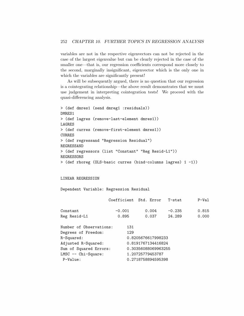
252 CHAPTER 10. FURTHER TOPICS IN REGRESSION ANALYSIS
variables are not in the respective eigenvectors can not be rejected in thecase of the largest eigenvalue but can be clearly rejected in the case of thesmaller one—that is, our regression coefficients correspond more closely tothe second, marginally insignificant, eigenvector which is the only one inwhich the variables are significantly present!
As will be subsequently argued, there is no question that our regressionis a cointegrating relationship—the above result demonstrates that we mustuse judgement in interpreting cointegration tests! We proceed with thequasi-differencing analysis.
> (def dmres1 (send dmreg1 :residuals))DMRES1> (def lagres (remove-last-element dmres1))LAGRES> (def curres (remove-first-element dmres1))CURRES> (def regressand "Regression Residual")REGRESSAND> (def regressors (list "Constant" "Reg Resid-L1"))REGRESSORS> (def rhoreg (OLS-basic curres (bind-columns lagres) 1 -1))
LINEAR REGRESSION
Dependent Variable: Regression Residual
Coefficient Std. Error T-stat P-Val
Constant -0.001 0.004 -0.235 0.815Reg Resid-L1 0.895 0.037 24.289 0.000
Number of Observations: 131Degrees of Freedom: 129R-Squared: 0.8205676617998233Adjusted R-Squared: 0.8191767134416824Sum of Squared Errors: 0.30356088069963255LMSC -- Chi-Square: 1.20725779453787P-Value: 0.2718758894595398

10.3. GENERALISED LEAST SQUARES 253
Breusch-Pagan -- Chi-Square: 0.32955957761872334P-Value: 0.565918539873963
Regression F-Statistic: 589.9339518949264P-Value: 0.0
RHOREG> (def rho (select (send rhoreg :coef-estimates) 1))> rho0.8951609929007297RHO> (def lagrm1 (remove-last-element rm1ca))LAGRM1> (def rm1 (remove-first-element rm1ca))RM1> (def drm1 (- rm1 (* rho lagrm1)))DRM1> (def lagrgdp (remove-last-element rgdpca))LAGRGDP> (def rgdp (remove-first-element rgdpca))RGDP> (def drgdp (- rgdp (* rho lagrgdp)))DRGDP> (def lagintr (remove-last-element cpapm1ca))LAGINTR> (def intr (remove-first-element cpapm1ca))INTR> (def dintr (- intr (* rho lagintr)))DINTR> (def regressand "Quasi-Difference of M1")REGRESSAND> (def regressors (list "Constant" "Quasi-Diff Intr" "Quasi-Diff RGDP"))REGRESSORS

254 CHAPTER 10. FURTHER TOPICS IN REGRESSION ANALYSIS
> (def GLSreg (OLS-basic drm1 (bind-columns dintr drgdp) 1 -1))
LINEAR REGRESSION
Dependent Variable: Quasi-Difference of M1
Coefficient Std. Error T-stat P-Val
Constant -0.153 0.044 -3.496 0.001Quasi-Diff Intr -0.015 0.002 -6.588 0.000Quasi-Diff RGDP 1.372 0.092 14.965 0.000
Number of Observations: 131Degrees of Freedom: 128R-Squared: 0.6856741695333268Adjusted R-Squared: 0.6807628284322851Sum of Squared Errors: 0.1204414962061645LMSC -- Chi-Square: 1.330055538584672P-Value: 0.24879533765399853Breusch-Pagan -- Chi-Square: 6.276881534139337P-Value: 0.04335033850785619Regression F-Statistic: 139.61037432075022P-Value: 0.0
QDREG
The coefficients of this regression have the expected signs and are highlystatistically significant. And there is no longer first-order serial correlationin the residuals. This implies that a non-spurious relationship between thereal money stock, interest rates and real income along lines suggested byeconomic theory surely exists—it is difficult to imagine that residuals con-taining no first-order autocorrelation could be non-stationary. As a matterof interest, however, we do a Phillips-Perron test on these regression resid-uals.

10.3. GENERALISED LEAST SQUARES 255
> (def qdres (send qdreg :residuals))QDRES> (ppunit qdres "QD-residuals" 1)
PHILLIPS-PERRON TEST --- QD-residualsLags Truncated at 1
Least Squares Estimates:
Constant -7.451810E-5 (2.682737E-3)Trend 4.510634E-5 (7.159764E-5)Lagged Y 9.740360E-2 (8.827513E-2)
R Squared: 1.319918E-2Sigma hat: 3.058516E-2Number of cases: 130Degrees of freedom: 127
Standard t-ratios:
Constant -0.027776893933704135Trend 0.6299976196924618Lagged Y = 0 1.1034092509913784Lagged Y = 1 -10.224809280151813
Least Squares Estimates:
Constant -5.189249E-5 (2.676170E-3)Lagged Y 0.100558 (8.792519E-2)
R Squared: 1.011526E-2Sigma hat: 3.051302E-2Number of cases: 130Degrees of freedom: 128
Standard t-ratios:
Constant -0.019390583804669008Lagged Y = 0 1.143671243141247Lagged Y = 1 -10.229633979287446
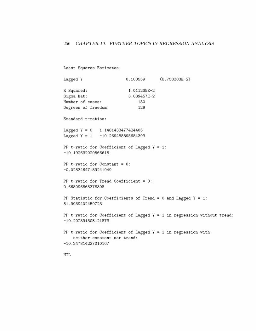
256 CHAPTER 10. FURTHER TOPICS IN REGRESSION ANALYSIS
Least Squares Estimates:
Lagged Y 0.100559 (8.758383E-2)
R Squared: 1.011235E-2Sigma hat: 3.039457E-2Number of cases: 130Degrees of freedom: 129
Standard t-ratios:
Lagged Y = 0 1.1481433477424405Lagged Y = 1 -10.269488895684393
PP t-ratio for Coefficient of Lagged Y = 1:-10.192632020566615
PP t-ratio for Constant = 0:-0.02834647189241949
PP t-ratio for Trend Coefficient = 0:0.668096865378308
PP Statistic for Coefficients of Trend = 0 and Lagged Y = 1:51.9939402459723
PP t-ratio for Coefficient of Lagged Y = 1 in regression without trend:-10.202391305121873
PP t-ratio for Coefficient of Lagged Y = 1 in regression withneither constant nor trend:
-10.247814227010167
NIL

10.3. GENERALISED LEAST SQUARES 257
> (ppunit qdres "QD-residuals" 5)
PHILLIPS-PERRON TEST --- QD-residualsLags Truncated at 5
Least Squares Estimates:
Constant -7.451810E-5 (2.682737E-3)Trend 4.510634E-5 (7.159764E-5)Lagged Y 9.740360E-2 (8.827513E-2)
R Squared: 1.319918E-2Sigma hat: 3.058516E-2Number of cases: 130Degrees of freedom: 127
Standard t-ratios:
Constant -0.027776893933704135Trend 0.6299976196924618Lagged Y = 0 1.1034092509913784Lagged Y = 1 -10.224809280151813
Least Squares Estimates:
Constant -5.189249E-5 (2.676170E-3)Lagged Y 0.100558 (8.792519E-2)
R Squared: 1.011526E-2Sigma hat: 3.051302E-2Number of cases: 130Degrees of freedom: 128
Standard t-ratios:
Constant -0.019390583804669008Lagged Y = 0 1.143671243141247Lagged Y = 1 -10.229633979287446
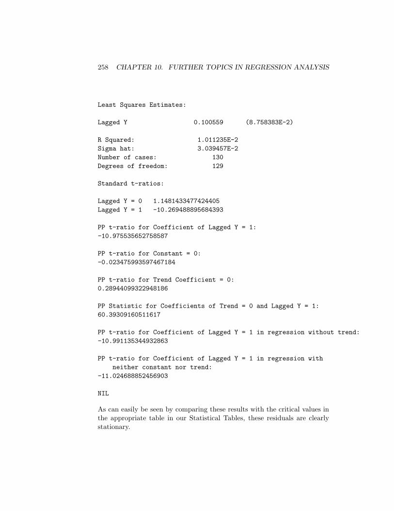
258 CHAPTER 10. FURTHER TOPICS IN REGRESSION ANALYSIS
Least Squares Estimates:
Lagged Y 0.100559 (8.758383E-2)
R Squared: 1.011235E-2Sigma hat: 3.039457E-2Number of cases: 130Degrees of freedom: 129
Standard t-ratios:
Lagged Y = 0 1.1481433477424405Lagged Y = 1 -10.269488895684393
PP t-ratio for Coefficient of Lagged Y = 1:-10.975535652758587
PP t-ratio for Constant = 0:-0.023475993597467184
PP t-ratio for Trend Coefficient = 0:0.28944099322948186
PP Statistic for Coefficients of Trend = 0 and Lagged Y = 1:60.39309160511617
PP t-ratio for Coefficient of Lagged Y = 1 in regression without trend:-10.991135344932863
PP t-ratio for Coefficient of Lagged Y = 1 in regression withneither constant nor trend:
-11.024688852456903
NIL
As can easily be seen by comparing these results with the critical values inthe appropriate table in our Statistical Tables, these residuals are clearlystationary.

10.3. GENERALISED LEAST SQUARES 259
The above procedure is, in fact, generalised least squares—it involvesspecification of the nature of the regression residuals and running a regres-sion based on that specification. Accordingly, essentially the same resultscan be obtained by defining the variance-covariance matrix of the residualsas
Ω = σ2
1 ρ ρ 2 ρ 3 · · · ρT−1
ρ 1 ρ · · · · · · ρT−2
ρ 2 ρ 1 · · · · · · ρT−3
ρ 3 · · · · · · · · · · · · · · ·· · · · · · · · · · · · · · · · · ·ρT−1 ρT−2 ρT−3 · · · · · · 1
where we can replace σ2 with σ2µ/(1− ρ2) with σ2
µ being the mean-squared-error of µt, the quasi-differenced-regression residual.10 We can reproducethe quasi-difference results to a close approximation using the calculationsin equations (10.10) and (10.11) and extensions thereof, with the mean-squared error from QDREG being our estimate of σ2
µ.Using ρ = 0.895, the value obtained from RHOREG above, we can use
the GLS function that I have written to obtain the result below. TheGLS function takes three arguments—in order, the dependent variable, thematrix of independent variables including the constant if one is desired andthe matrix Ω calculated using the above values assigned to ρ and σ2
µ. Ourfirst task is to construct an estimate of Ω. We continue to work in theprevious XLispStat workspace.
> (def reg1df (send dmreg1 :df))REG1DF> (def reg1mse (/ (sum (^ dmres1 2)) reg1df))REG1MSE> (def bigT (length rm1ca))BIGT> (def OMEG (identity-matrix bigT))OMEG> (dotimes (i bigT)(dotimes (j (- bigT i))(setf (aref OMEG i (+ j i))(^ rho j))) ; end dotimes j) ; end dotimes iNIL
10This result can be obtained by simply taking the variance of equation (10.13), keepingin mind that the current and lagged residuals must have the same variance.

260 CHAPTER 10. FURTHER TOPICS IN REGRESSION ANALYSIS
> (dotimes (i bigT)(setf (aref OMEG i i) 0.5)) ; end dotimes iNIL> (def OMEGA (* (/ Qdifmse (- 1 (^ rho 2)))(+ (transpose OMEG) OMEG)))OMEGA> (def regressand "Real M1")REGRESSAND> (def regressors (list "Constant" "1-mo Com Pap Rate" "Real GDP"))REGRESSORS> (def const (repeat 1 bigT))CONST> (def Xmat (bind-columns const cpapm1ca rgdpca))XMAT> (GLS rm1ca Xmat omega)
GENERALISED LEAST SQUARES REGRESSION
Dependent Variable: Real M1
Coefficient Std. Error T-stat P-Val
Constant -0.228 0.317 -0.720 0.4721-mo Com Pap Rate -0.015 0.002 -6.682 0.000Real GDP 1.107 0.071 15.654 0.000
Number of Observations: 132Degrees of Freedom: 129R-Squared: 0.8366306285697146
NIL
The coefficient of the interest rate is the same as in the quasi-differencedregression while the coefficient of real income is about 20 percent smaller.Both are highly significant.
The usual procedure at this point is to optimise the result by tryingvalues of RHO ranging between 0 and 1 and picking the value that minimisesthe sum of squared errors of the quasi-differenced regression—our use of theabove GLS regression is purely illustrative. The first step is to use the RHO

10.3. GENERALISED LEAST SQUARES 261
values [.1 .2 .3 .4 .5 .6 .7 .8 .9] and then, having selected the value thatgives the minimum sum of squared error, iterate more finely in differencesof .01 and .001 with in a range of .2 around that maximum to zero-in ona more exact maximum value of RHO.11 In our case, it turns out that theminimum sum of squared errors occurs at .9 in the first round and thendiminishes as the selected RHO value is increased above that level. Themaximum occurs when RHO = 1 that is when we run first-differences insteadof quasi-differences. This implies that the error term in our initial (DMREG1)regression has a unit root, a result that conforms to our cointegration test onthe residuals of that regression and is not grossly violated by our Johansencointegration test. To ensure that this result is not due to programmingerrors, I ran the test in the commercial program SHAZAM using exactlythe same data. Using maximum likelihood estimation, SHAZAM settledupon a value of RHO of .99122 and using a Cochrane-Orcutt approach theoptimum value was .99653. We obtain very similar values for the coefficientsto those obtained by SHAZAM for both of these RHO values. Our result forRHO = .99122 is
> (GLS rm1ca Xmat omega)
GENERALISED LEAST SQUARES REGRESSION
Dependent Variable: Real M1
Coefficient Std. Error T-stat P-Val
Constant 0.817 0.811 1.008 0.3141-mo Com Pap Rate -0.011 0.002 -5.050 0.000Real GDP 0.893 0.180 4.961 0.000
Number of Observations: 132Degrees of Freedom: 129R-Squared: 0.6204408078922425
NIL
11This approach goes back to the work of Clifford Hildreth and John Y. Lu, DemandRelations with Autocorrelated Disturbances, Agriculture Experiment Station TechnicalBulletin 276, Michigan State University, East-Lansing, Michigan, 1960. An alternativeapproach, due to D. Cochrane and Guy H. Orcutt, “Application of Least-Squares Regres-sion to Relationships Containing Auto-correlated Error Terms,” Journal of the AmericanStatistical Association, Vol. 44, No. 1 (1949), 32-61, involves interaction around the ini-tial value of RHO obtained in our regression RHOREG above. Of these two approaches, theHildreth-Lu approach is probably best because there is less chance of ending up at a localrather than global maximum.
262 CHAPTER 10. FURTHER TOPICS IN REGRESSION ANALYSIS
The corresponding coefficients obtained by SHAZAM were 0.83252 for theconstant, -0.010737 for the interest rate and 0.88998 for real GDP. SHAZAMcannot settle on a value of RHO as large as 1 because the variance of theresidual of the counterpart to our DMREG1 will become infinite—that is, theresidual becomes a random walk.
One has to conclude that, apart from the fact that the signs of the co-efficients are correct, the above results are essentially nonsense! It makesno sense for the residual of the demand function for money to be a randomwalk, since that would imply that holding the interest rate, real incomeand the nominal quantity of money constant, the price level can eventu-ally approach zero or infinity! The fact that the signs of the interest rateand income variables are the expected ones and those variables are signifi-cant in quasi-differenced and first-differenced regressions suggests that theremust be a stable demand function for money having the conventionally ex-pected characteristics. Thus, while the above results illustrate how one cancalculate the statistics we obtain, it makes no sense to use this analyticaltechnique for analysing the demand for money.
Indeed, as Jack Carr showed many years ago, the practice of using thesetechniques to rid the residuals of a model of serial correlation focuses on thewrong issues.12 The residuals are serially correlated because autocorrelatedvariables are left out of the regression or because the form of the regressionfunction is incorrect. The focus should therefore be on finding the correctexplanatory variables or adopting a different, perhaps non-linear, regressionfunction. It is not clear that our estimates of the regression coefficients willbe more accurate when we quasi-difference for first-order serial correlation(or similarly handle higher-order serial correlation) in the regression resid-uals than if we go with the original coefficient estimates—in the case ofleft-out variables, it will depend on the direction of the correlation of thesevariables with the regression residual, with the included variables and withthe dependent variable. The best bet when confronted by serial correlationin regression residuals arising from an unknown source, or one that cannotbe dealt with, is probably to adopt HAC coefficient-standard-errors and livewith the observed coefficients as rough estimates.
Indeed, there is a literature that attempts to provide an economic expla-nation the observed serial correlation in demand-function-for-money resid-uals. The problem is that a change in the nominal stock of money willsignificantly affect prices, and hence the real money stock, only after some
12See Jack Carr, “A Suggestion for the Treatment of Serial Correlation: A Case inPoint,” Canadian Journal of Economics, Vol. 2, May 1972, 301-306.

10.3. GENERALISED LEAST SQUARES 263
time has elapsed. Serial correlation in the residuals will therefore be a con-sequence of this adjustment process. The way to deal with this serial cor-relation is therefore to incorporate into the regression equation a model ofthe adjustment process.13
10.3.3 Seemingly Unrelated Regression Techniques
One use of generalised least squares for which there is often substantial sup-port from economic theory involves systems estimation that uses seeminglyunrelated regression techniques. Suppose our model consists of two equa-tions the can be represented in a form suitable for OLS estimation. Becausethey are part of the same model the residuals of these two estimating equa-tions may be correlated—left out variables can affect both equations. If thisis the case, we can take advantage of this fact to increase the efficiency ofour estimates.
Suppose that the two equations are
y1 = X1 β1 + ε1 (10.15)y2 = X2 β2 + ε2 (10.16)
where y1 and y2 are T × 1 column vectors, T being the number of obser-vations, X1 and X1 are m1 × T and m2 × T matrices, with m1 and m2
being the number of independent variables including the constant in thetwo equations, β1 and β1 are the m1 × 1 and m2 × 1 vectors of coefficientsand ε1 and ε2 are the T × 1 vectors of residuals. The matrices X1 and X2
may contain many of the same variables, but cannot be identical.14 Whenwe stack these equations as follows
[y1
y2
]=
[X1 00 X2
] [β1
β2
]+
[ε1
ε2
](10.17)
and estimate them by OLS as a system, it may be inappropriate to assume,even when homoskedasticity holds, that the variance-covariance matrix ofthe true vector of errors is of the form[
σ 21 I 00 σ 2
2 I
]
13For analysis along these lines, see Jack Carr and Michael R. Darby, “The Role ofMoney Supply Shocks in the Short-run Demand for Money,” Journal of Monetary Eco-nomics, Vol. 8, No. 2 (September), 1981, 183-199.
14If the independent variables are the same in the two equations, nothing will be gainedby using the techniques applied here—the equations can just as well be estimated sepa-rately by OLS.
264 CHAPTER 10. FURTHER TOPICS IN REGRESSION ANALYSIS
where σ 21 and σ 2
2 are residual variances of the two equations,
ε ′1 ε1
T −m1and
ε ′2 ε2
T −m2.
It is probably the case that σ12 is non-zero.Accordingly, it is appropriate to obtain estimates of σ 2
1 , σ 22 and σ12 in
the usual fashion after estimating the two equations separately using OLS,and construct the matrix
Ω =
[s 21 I s12 I
s12 I s 22 I
]
and estimate the two-equation system by GLS, calculating (10.10) and (10.11)and related statistics with our GLS function.
It is useful to apply these techniques to the issues outlined in the firstsection of this chapter—the problem of whether the classical price-specie-flow theory or a modern portfolio approach best describes the operation ofthe commodity standard in the U.S. during the years 1820 to 1860. It wasnoted there that the price-specie-flow mechanism assumes that the balanceof payments surplus is additively determined by the balance of trade andthe net capital flow, where the latter treated as positively related to theratio of the U.S. to the rest-of-world interest rate. It should therefore bethe case that the effects of changes in the real exchange rate and U.S. andforeign incomes on the balance of payments should be identical to the effectsof these variables on the balance of payments.
First we load the data and run the two equations separately using OLS.Following our earlier results, we estimate the balance of trade as a functionof the real exchange rate and U.S. and rest-of-world incomes and the balanceof payments as a function of these same variables plus several proxies forthe long-term net capital inflow into the U.S., the real debt service balanceand the ratio of U.S. to foreign interest rates.
> (load "addfuncs.lsp"); loading addfuncs.lspT> (load "antbdata.lsp"); loading antbdata.lspT

10.3. GENERALISED LEAST SQUARES 265
> (variables)(INTDIF NPRUSROW NRESFLOW REXUSROW ROWPL ROWRGNP RRESFLOW UKCONSOLUKOMDR USCPIBDS USIPDB USMM USNCIDSB USNGNPB USNMONT USRCANI USRDSBUSRGNPB USRGNPBI USRMON USRNCIXS USROWRN USRPLS USRRMP USRSPRESUSSERV USSINT USSPECXP USSPTC USTBN USTBNGS USTBRGS USTOTN USUKEXRBUSUKEXRP USUKMPO YEAR)> (def consterm (repeat 1 41))CONSTERM> (def idepvarbot (bind-columns consterm rexusrow usrgnpbi rowrgnp))IDEPVARBOT> (def idepvarbop (bind-columns consterm rexusrow usrgnpbi rowrgnpusrpls usrcani usrrmp usrdsb intdif))IDEPVARBOP> (def ustbrgs (remove-first-element ustbrgs))USTBRGS> (def rresflow (remove-first-element rresflow))RRESFLOW> (def regressand "Real Trade Balance")REGRESSAND> (def regressors (list "Constant " "Real Exch Rate" "US Real Income""ROW Real Income"))REGRESSORS> (def botreg0 (OLS-basic ustbrgs idepvarbot 0 -1))
LINEAR REGRESSION
Dependent Variable: Real Trade Balance
Coefficient Std. Error T-stat P-Val
Constant 20.682 38.882 0.532 0.598Real Exch Rate -1.267 0.261 -4.858 0.000US Real Income -2.099 0.315 -6.657 0.000ROW Real Income 2.976 0.613 4.853 0.000
Number of Observations: 40Degrees of Freedom: 36R-Squared: 0.6239916887697452

266 CHAPTER 10. FURTHER TOPICS IN REGRESSION ANALYSIS
Adjusted R-Squared: 0.5926576628338907Sum of Squared Errors: 10455.051622163453LMSC -- Chi-Square: 0.008244934976584888P-Value: 0.9276502193756687Breusch-Pagan -- Chi-Square: 4.728292600020851P-Value: 0.31632912615677045Regression F-Statistic: 19.914188175089578P-Value: 8.848164156916027E-8
BOTREG0> (def regressand "Real Reserve Flow")REGRESSAND> (def regressors (list "Constant " "Real Exch Rate" "US Real Income""ROW Real Income" "Pub Land Sales" "Canal Inv" "Rail Mileage""Net Rep Earn" "ST Int Diff"))REGRESSORS> (def bopreg0 (OLS-basic rresflow idepvarbop 0 -1))
LINEAR REGRESSION
Dependent Variable: Real Reserve Flow
Coefficient Std. Error T-stat P-Val
Constant -26.887 80.357 -0.335 0.740Real Exch Rate 1.287 0.603 2.136 0.041US Real Income 3.346 1.083 3.088 0.004ROW Real Income -3.577 1.245 -2.872 0.007Pub Land Sales -0.002 0.001 -1.608 0.118Canal Inv 0.020 1.862 0.011 0.992Rail Mileage -0.004 0.002 -1.738 0.092Net Rep Earn 0.722 2.575 0.281 0.781ST Int Diff 6.059 7.351 0.824 0.416
Number of Observations: 40Degrees of Freedom: 31R-Squared: 0.3308652691782614Adjusted R-Squared: 0.15818533864361928
10.3. GENERALISED LEAST SQUARES 267
Sum of Squared Errors: 25086.14724575851LMSC -- Chi-Square: 6.194712545745064P-Value: 0.012813253407204406
Breusch-Pagan -- Chi-Square: 18.43904085444853P-Value: 0.03040834955072791
Regression F-Statistic: 1.9160609351292557P-Value: 0.09308907718049675
BOPREG0
We use the OLS-basic function here because we are not interested in pro-ducing HAC coefficient standard errors. Next, we calculate the variancesand covariances of the residuals of the two equations and use these to con-struct our Ω, which we will call SUROMEGA.
> (def resbot0 (send botreg0 :residuals))RESBOT0> (def resbop0 (send bopreg0 :residuals))RESBOP0> (def covbtp (covariance resbot0 resbop0))COVBTP> (def varbt (variance resbot0))VARBT> (def varbp (variance resbop0))VARBP> (def upleft (* varbt (identity-matrix 40)))UPLEFT> (def lorite (* varbp (identity-matrix 40)))LORITE> (def offdiag (* covbtp (identity-matrix 40)))OFFDIAG> (def topSUROMEGA (bind-columns upleft offdiag))TOPSUROMEGA> (def botSUROMEGA (bind-columns offdiag lorite))BOTSUROMEGA> (def SUROMEGA (bind-rows topSUROMEGA botSUROMEGA))SUROMEGA
Then we calculate the stacked y-vector and X-matrix and apply the GLSfunction.
268 CHAPTER 10. FURTHER TOPICS IN REGRESSION ANALYSIS
> (def zeromatt (make-array ’(40 9) :initial-element 0))ZEROMATT> (def topmat (bind-columns idepvarbot zeromatt))TOPMAT> (def zeromatp (make-array ’(40 4) :initial-element 0))ZEROMATP> (def botmat (bind-columns zeromatp idepvarbop))BOTMAT> (def SURXmat (bind-rows topmat botmat))SURXMAT> (def SURYvar (append ustbrgs rresflow))SURYVAR> (def regressand "SUR: Real Trade Balance (Top) // Real Net CapitalInflow")REGRESSAND> (def regressors (list "Constant" "Real Exch Rate" "US Real Income""ROW Real Income" "Constant" "Real Exch Rate" "US Real Income""ROW Real Income" "Pub Land Sales" "Canal Inv" "Rail Mileage" "Net Rep Earn""ST Int Diff"))REGRESSORS> (GLS SURYvar SURXmat SUROMEGA)
GENERALISED LEAST SQUARES REGRESSION
Dependent Variable: SUR: Real Trade Balance (Top) // Real Net CapitalInflow
Coefficient Std. Error T-stat P-Val
Constant 20.682 37.356 0.554 0.580Real Exch Rate -1.267 0.251 -5.057 0.000US Real Income -2.099 0.303 -6.929 0.000ROW Real Income 2.976 0.589 5.051 0.000Constant -23.786 71.569 -0.332 0.740Real Exch Rate 1.256 0.536 2.341 0.019US Real Income 3.297 0.964 3.421 0.001ROW Real Income -3.573 1.109 -3.221 0.001Pub Land Sales -0.002 0.001 -1.718 0.086Canal Inv 0.093 1.656 0.056 0.955Rail Mileage -0.004 0.002 -1.918 0.055
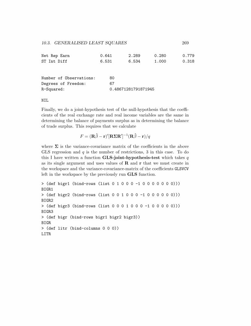
10.3. GENERALISED LEAST SQUARES 269
Net Rep Earn 0.641 2.289 0.280 0.779ST Int Diff 6.531 6.534 1.000 0.318
Number of Observations: 80Degrees of Freedom: 67R-Squared: 0.48671281791871945
NIL
Finally, we do a joint-hypothesis test of the null-hypothesis that the coeffi-cients of the real exchange rate and real income variables are the same indetermining the balance of payments surplus as in determining the balanceof trade surplus. This requires that we calculate
F = (Rβ − r)′[RΣR′]−1(Rβ − r)/q
where Σ is the variance-covariance matrix of the coefficients in the aboveGLS regression and q is the number of restrictions, 3 in this case. To dothis I have written a function GLS-joint-hypothesis-test which takes qas its single argument and uses values of R and r that we must create inthe workspace and the variance-covariance-matrix of the coefficients GLSVCVleft in the workspace by the previously run GLS function.
> (def bigr1 (bind-rows (list 0 1 0 0 0 -1 0 0 0 0 0 0 0)))BIGR1> (def bigr2 (bind-rows (list 0 0 1 0 0 0 -1 0 0 0 0 0 0)))BIGR2> (def bigr3 (bind-rows (list 0 0 0 1 0 0 0 -1 0 0 0 0 0)))BIGR3> (def bigr (bind-rows bigr1 bigr2 bigr3))BIGR> (def litr (bind-columns 0 0 0))LITR
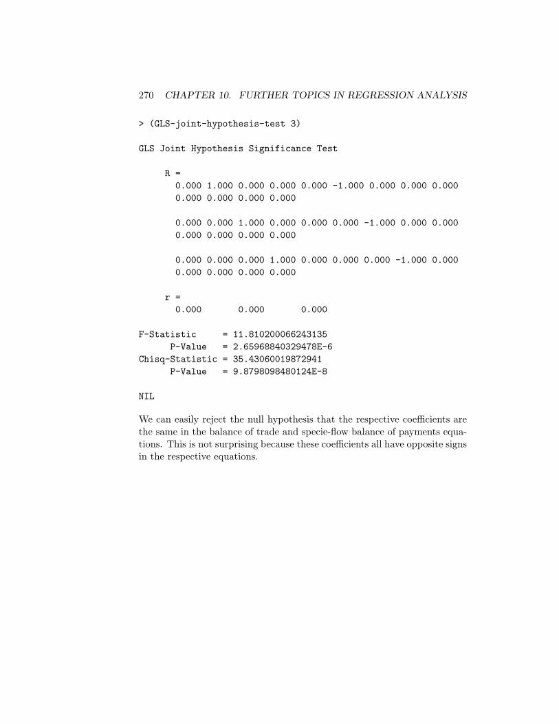
270 CHAPTER 10. FURTHER TOPICS IN REGRESSION ANALYSIS
> (GLS-joint-hypothesis-test 3)
GLS Joint Hypothesis Significance Test
R =0.000 1.000 0.000 0.000 0.000 -1.000 0.000 0.000 0.0000.000 0.000 0.000 0.000
0.000 0.000 1.000 0.000 0.000 0.000 -1.000 0.000 0.0000.000 0.000 0.000 0.000
0.000 0.000 0.000 1.000 0.000 0.000 0.000 -1.000 0.0000.000 0.000 0.000 0.000
r =0.000 0.000 0.000
F-Statistic = 11.810200066243135P-Value = 2.65968840329478E-6
Chisq-Statistic = 35.43060019872941P-Value = 9.8798098480124E-8
NIL
We can easily reject the null hypothesis that the respective coefficients arethe same in the balance of trade and specie-flow balance of payments equa-tions. This is not surprising because these coefficients all have opposite signsin the respective equations.

Chapter 11
Vector AutoregressionAnalysis
We now turn to vector autoregression analysis. For background, readersshould work through pages 291-353 of the Enders textbook, and pages 257-372 of the Hamilton book. They should also read sections of a book byHelmut Lutkepohl.1 A vector autoregression (VAR) is a set of regressions ofeach series in a vector of time series on lagged values both of itself and theother series in that vector. Consider the following economic model with twovariables, y1 and y2, each of which depends on itself lagged, on the currentand lagged values of the other variable and on a iid error term:
y1(t) = v10 + v12 y2(t) + a11 y1(t−1) + a12 y2(t−2) + e1(t) (11.1)
y2(t) = v20 + v21 y1(t) + a21 y1(t−1) + a22 y2(t−2) + e2(t) (11.2)
This system can be written in matrix notation as[
y1(t)
y2(t)
]=
[v10
v20
]+
[0 v12
v21 0
] [y1(t)
y2(t)
]
+
[a11 a12
a21 a22
] [y1(t−1)
y2(t−1)
]+
[e1(t)
e2(t)
](11.3)
or, in general matrix notation with m variables and p lags we would write
1See Helmut Lutkepohl Introduction to Multiple Time Series Analysis, Springer-Verlag,1991, pages 9-27, 43-58 and 97-117.
271

272 CHAPTER 11. VECTOR AUTOREGRESSION ANALYSIS
yt = v + A0 yt + A1 yt−1 + A2 yt−2 + A3 yt−3 + · · ·+ · · ·+ Ap yt−p + et (11.4)
where yt, v and et are m × 1 column vectors and A0, A1, A2, · · · Ap arem×m matrices of coefficients. The vector et is a m-element vector of whitenoise residuals that satisfies Eetet
′ = D, where D is a diagonal matrix. Anappropriate scaling of the elements of y would make D an identity matrix.
Equations (11.1) and (11.2), which are called a structural VAR or aprimitive system, can be solved simultaneously to yield the reduced form orstandard form of the VAR:
y1(t) = b10 + b11 y1(t−1) + b12 y2(t−2) + u1(t) (11.5)y2(t) = b20 + b21 y1(t−1) + b22 y2(t−2) + u2(t) (11.6)
or[
y1(t)
y2(t)
]=
[b10
b20
]+
[b11 b12
b21 b22
] [y1(t−1)
y2(t−1)
]+
[u1(t)
u2(t)
](11.7)
where
b10 =v10 + v12 v20
1− v12 v21
b11 =v12 a11 + a21
1− v12 v21
b12 =a12 + v12 a22
1− v12 v21
b20 =v20 + v21 v10
1− v12 v21
b21 =a21 + v21 a11
1− v12 v21
b22 =v21 a12 + a22
1− v12 v21
and
u1(t) =1
1− v12 v21
[e1(t) + v12 e2(t)
]
u2(t) =1
1− v12 v21
[v21 e1(t) + e2(t)
].

273
In the general m variable case with p lags we have
(I−A0)yt = v + A1 yt−1 + A2 yt−2 + A3 yt−3 + · · ·· · ·+ AP yt−p + et (11.8)
which reduces to
yt = (I−A0)−1v + (I−A0)−1A1 yt−1 + (I−A0)−1A2 yt−2
+(I−A0)−1A3 yt−3 + · · ·+ (I−A0)−1AP yt−p
+(I−A0)−1et. (11.9)
Letting b = (I − A0)−1v, B1 = (I − A0)−1A1, B2 = (I − A0)−1A2, · · ·etc., and ut = (I−A0)−1 et we can write the VAR in standard form in thegeneral case as
yt = b + B1 yt−1 + B2 yt−2 + B3 yt−3 + · · ·· · ·+ BP yt−p + ut. (11.10)
All this assumes, of course, that the matrix (I−A0) has an inverse. Giventhat Eetet
′ = D, the variance-covariance matrix of the vector of residualsut equals
Ω = Eutut′
= E[(I−A0)−1et][(I−A0)−1et]′= E[(I−A0)−1]etet
′[(I−A0)−1]′= [(I−A0)−1]Eetet
′[(I−A0)−1]′
= [(I−A0)−1]D [(I−A0)−1] ′.
The equations in (11.10) can be estimated by ordinary least squares—because the independent variables in all equations are the same, there is noefficiency gain by estimating these equations as a system using the seeminglyunrelated regression technique.
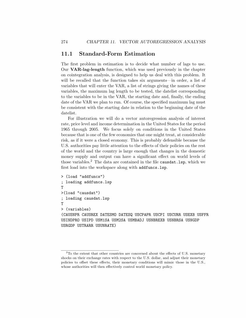
274 CHAPTER 11. VECTOR AUTOREGRESSION ANALYSIS
11.1 Standard-Form Estimation
The first problem in estimation is to decide what number of lags to use.Our VAR-lag-length function, which was used previously in the chapteron cointegration analysis, is designed to help us deal with this problem. Itwill be recalled that the function takes six arguments—in order, a list ofvariables that will enter the VAR, a list of strings giving the names of thesevariables, the maximum lag length to be tested, the datelist correspondingto the variables to be in the VAR, the starting date and, finally, the endingdate of the VAR we plan to run. Of course, the specified maximum lag mustbe consistent with the starting date in relation to the beginning date of thedatelist.
For illustration we will do a vector autoregression analysis of interestrate, price level and income determination in the United States for the period1965 through 2005. We focus solely on conditions in the United Statesbecause that is one of the few economies that one might treat, at considerablerisk, as if it were a closed economy. This is probably defensible because theU.S. authorities pay little attention to the effects of their policies on the restof the world and the country is large enough that changes in the domesticmoney supply and output can have a significant effect on world levels ofthose variables.2 The data are contained in the file causdat.lsp, which wefirst load into the workspace along with addfuncs.lsp.
> (load "addfuncs"); loading addfuncs.lspT>(load "causdat"); loading causdat.lspT> (variables)(CAUSNPR CAUSREX DATESMO DATESQ USCPAPR USCPI USCURR USEXB USFFRUSINDPRO USIPD USM1SA USM2SA USMBADJ USNBREXB USNBRSA USNGDPUSRGDP USTRARR USUNRATE)
2To the extent that other countries are concerned about the effects of U.S. monetaryshocks on their exchange rates with respect to the U.S. dollar, and adjust their monetarypolicies to offset these effects, their monetary conditions will mimic those in the U.S.,whose authorities will then effectively control world monetary policy.
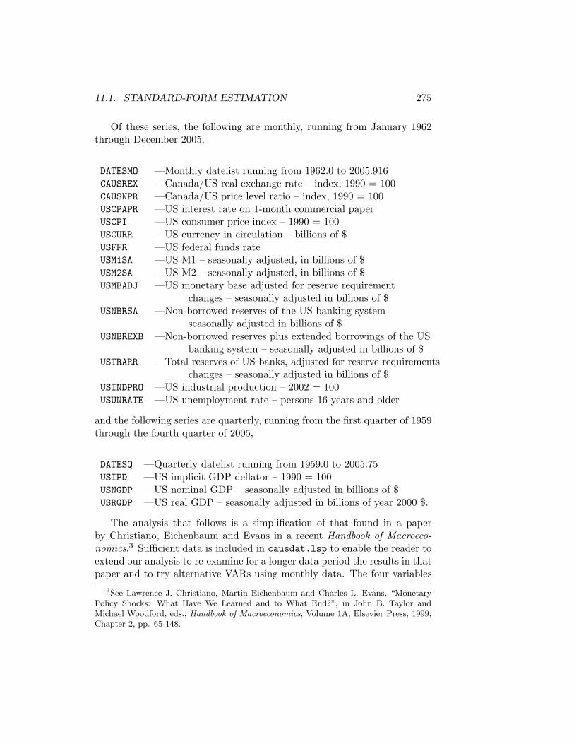
11.1. STANDARD-FORM ESTIMATION 275
Of these series, the following are monthly, running from January 1962through December 2005,
DATESMO —Monthly datelist running from 1962.0 to 2005.916CAUSREX —Canada/US real exchange rate – index, 1990 = 100CAUSNPR —Canada/US price level ratio – index, 1990 = 100USCPAPR —US interest rate on 1-month commercial paperUSCPI —US consumer price index – 1990 = 100USCURR —US currency in circulation – billions of $USFFR —US federal funds rateUSM1SA —US M1 – seasonally adjusted, in billions of $USM2SA —US M2 – seasonally adjusted, in billions of $USMBADJ —US monetary base adjusted for reserve requirement
changes – seasonally adjusted in billions of $USNBRSA —Non-borrowed reserves of the US banking system
seasonally adjusted in billions of $USNBREXB —Non-borrowed reserves plus extended borrowings of the US
banking system – seasonally adjusted in billions of $USTRARR —Total reserves of US banks, adjusted for reserve requirements
changes – seasonally adjusted in billions of $USINDPRO —US industrial production – 2002 = 100USUNRATE —US unemployment rate – persons 16 years and older
and the following series are quarterly, running from the first quarter of 1959through the fourth quarter of 2005,
DATESQ —Quarterly datelist running from 1959.0 to 2005.75USIPD —US implicit GDP deflator – 1990 = 100USNGDP —US nominal GDP – seasonally adjusted in billions of $USRGDP —US real GDP – seasonally adjusted in billions of year 2000 $.
The analysis that follows is a simplification of that found in a paperby Christiano, Eichenbaum and Evans in a recent Handbook of Macroeco-nomics.3 Sufficient data is included in causdat.lsp to enable the reader toextend our analysis to re-examine for a longer data period the results in thatpaper and to try alternative VARs using monthly data. The four variables
3See Lawrence J. Christiano, Martin Eichenbaum and Charles L. Evans, “MonetaryPolicy Shocks: What Have We Learned and to What End?”, in John B. Taylor andMichael Woodford, eds., Handbook of Macroeconomics, Volume 1A, Elsevier Press, 1999,Chapter 2, pp. 65-148.

276 CHAPTER 11. VECTOR AUTOREGRESSION ANALYSIS
in our VAR are real GDP, the implicit GDP deflator, the 1-month corporatepaper interest rate, and the stock of M1, with all but the interest rate inlogarithms and the interest rate expressed as a fraction of unity rather thanin annual percentage terms. As a preliminary step, we must be convert themoney and interest rate series to quarterly averages and shorten the quar-terly series to be consistent with the monthly ones. All the calculations thatfollow can be found in the batch file VARbatch.lsp.
> (def uscpapr (m2q-avg uscpapr 0 1962.0 2005.75))USCPAPR> (def usm1 (m2q-avg usm1sa 0 1962.0 2005.75))USM1> (def usrgdp (remove-first 12 usrgdp))USRGDP> (def usipd (remove-first 12 usipd))USIPD> (def datesq (remove-first 12 datesq))DATESQ> (def logrgdp (remove-first 4 (log usrgdp)))LOGRGDP> (def logm1 (remove-first 4 (log usm1)))
LOGM1> (def logipd (remove-first 4 (log usipd)))LOGIPD> (def intrate (/ (remove-first 4 (copy-list uscpapr)) 100))INTRATE> (def newdates (remove-first 4 datesq))NEWDATES
Our four variables, LOGRGDP, INTRATE, LOGIPD and LOGM1 now begin at date1963.0. We now apply the VAR-lag-length function.
> (def varlist (list logrgdp logipd intrate logm1))VARLIST> (def varnames (list "LOGRGDP" "LOGIPD" "INTRATE" "LOGM1"))VARNAMES> (VAR-lag-length varlist varnames 8 newdates 1965.0 2005.75)

11.1. STANDARD-FORM ESTIMATION 277
LAG SELECTION INFORMATION
Variables are (LOGRGDP LOGIPD INTRATE LOGM1)
Degrees of Freedom Data Points Less LR-TestLag Per Equation All Parameters PVal AIC BIC
8 131 524 -6676.32 -6267.147 135 540 0.001 -6685.92 -6326.336 139 556 0.012 -6702.32 -6392.335 143 572 0.000 -6686.08 -6425.694 147 588 0.000 -6680.62 -6469.833 151 604 0.000 -6670.53 -6509.332 155 620 0.000 -6642.52 -6530.921 159 636 0.000 -6443.18 -6381.18
When doing Johansen cointegration tests 2 additional degreesof freedom per equation will be lost, reducing the datapoints minus total parameters estimated by 8
NIL
The BIC suggests that 2 lags are appropriate, the AIC suggests 6 lags and theLR-test suggests even more than 6 lags. For simplicity, we follow Christiano,Eichenbaum and Evans and settle on 4 lags.
I have written two functions that can be used to estimate a standard-formVAR. The first, VAR-setup, sets up and runs the VAR and leaves a numberof important objects in the workspace for subsequent use. The second VAR-run-standard-form calls the previous function and writes relevant resultsto the screen along with tests of the significance of the lagged values of eachof the variables in each equation. This latter function enables us to observeand analyse the standard-form results. Both of the above functions take thesame arguments—(1) a list of the variables ordered appropriately for anysubsequent Choleski decomposition, (2) the number of lags, (3) the datelistto which the variables conform, (4) the beginning date of the VAR, and (5)the ending date. Obviously, the beginning and ending dates and the numberof lags must be consistent with the datelist.
The VAR-setup function leaves some very important variables in theworkspace. First, it leaves a list of the lists that represent the variables in

278 CHAPTER 11. VECTOR AUTOREGRESSION ANALYSIS
the VAR, called xlists. Second, it leaves a list of matrices of the laggedvalues of the variables, called xmats. Third, it leaves a list containing thelists of coefficients of the constant and the lagged values of the variablesproduced by the standard-form regressions, called coefslists, a list calledVCVcoefslist giving the variance-covariance matrices of the coefficients,and three additional aptly-named objects, nobs, numlags, numvars anddates. The latter is a datelist representing the dates over which the VAR isrun. The function also leaves a list of the lists of residuals from the regres-sions, residslists. And, finally, it leaves a list called lagslists whichcontains lists of the lagged values of the variables associated with the firstobservations of the series in the VAR. The elements of all the above listshave the same ordering as the ordering in the list of variables given as anargument in the function. Most of these lists will ultimately be required insubsequent bootstrapping used to obtain confidence limits. This functionprints nothing to the screen or to file—its purpose is to leave objects in theworkspace that can be used by subsequent functions.
The VAR-run-standard-form function calls the VAR-setup function(as previously noted, it takes the same arguments as that function) and usesthe resulting objects in the workspace to run the standard-form regressionsusing the OLS-basic function, printing out the results. It requires thatthree additional objects be present in the workspace, a list of strings calledregressands giving the names of the variables in the VAR, a list of stringscalled regressors giving the names of the regressors, including the constantand the lagged values of each variable in the correct order (this list willbe the same for all the standard-form regressions), and a list of stringscalled varnames giving shortened names for the regressands that are eightor less capitalised characters long. No adjustments for heteroskedasticityand autocorrelation in the residuals are made. Finally, the function doesF-tests of the significance of the blocks of lags of each variable in eachequation. To do this, it calls my VAR-block-lag-significance function,which takes no arguments. In situations where we are not interested in theactual coefficients of the standard form regressions but only in whether theblocks of lags of the variables are statistically significant, we can simply runthe VAR-setup function followed by the VAR-block-lag-significancefunction, bypassing the VAR-run-standard-form function and requiringonly varnames in the workspace.
Continuing in the above workspace, we now run the VAR-run-standard-form function after setting up the lists of variable names it requires.
> (def regressands (list "Log RGDP" "Log Price Level" "Interest Rate""Log of M1"))REGRESSANDS
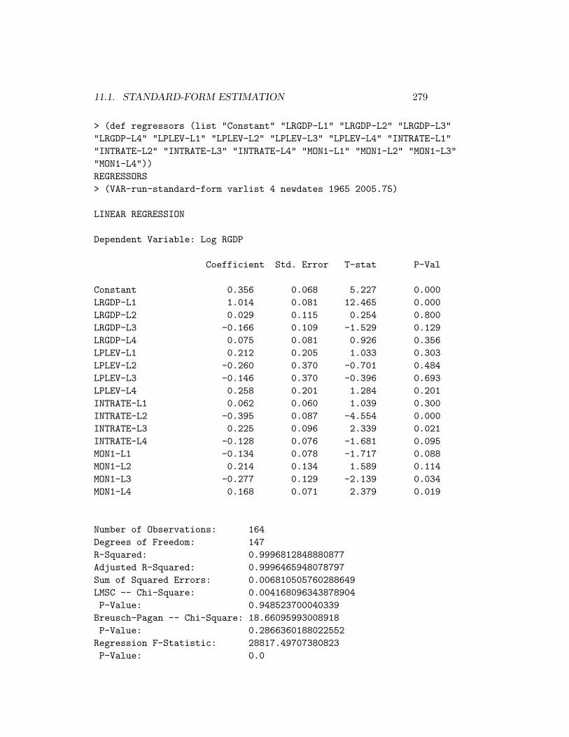
11.1. STANDARD-FORM ESTIMATION 279
> (def regressors (list "Constant" "LRGDP-L1" "LRGDP-L2" "LRGDP-L3""LRGDP-L4" "LPLEV-L1" "LPLEV-L2" "LPLEV-L3" "LPLEV-L4" "INTRATE-L1""INTRATE-L2" "INTRATE-L3" "INTRATE-L4" "MON1-L1" "MON1-L2" "MON1-L3""MON1-L4"))REGRESSORS> (VAR-run-standard-form varlist 4 newdates 1965 2005.75)
LINEAR REGRESSION
Dependent Variable: Log RGDP
Coefficient Std. Error T-stat P-Val
Constant 0.356 0.068 5.227 0.000LRGDP-L1 1.014 0.081 12.465 0.000LRGDP-L2 0.029 0.115 0.254 0.800LRGDP-L3 -0.166 0.109 -1.529 0.129LRGDP-L4 0.075 0.081 0.926 0.356LPLEV-L1 0.212 0.205 1.033 0.303LPLEV-L2 -0.260 0.370 -0.701 0.484LPLEV-L3 -0.146 0.370 -0.396 0.693LPLEV-L4 0.258 0.201 1.284 0.201INTRATE-L1 0.062 0.060 1.039 0.300INTRATE-L2 -0.395 0.087 -4.554 0.000INTRATE-L3 0.225 0.096 2.339 0.021INTRATE-L4 -0.128 0.076 -1.681 0.095MON1-L1 -0.134 0.078 -1.717 0.088MON1-L2 0.214 0.134 1.589 0.114MON1-L3 -0.277 0.129 -2.139 0.034MON1-L4 0.168 0.071 2.379 0.019
Number of Observations: 164Degrees of Freedom: 147R-Squared: 0.9996812848880877Adjusted R-Squared: 0.9996465948078797Sum of Squared Errors: 0.006810505760288649LMSC -- Chi-Square: 0.004168096343878904P-Value: 0.948523700040339
Breusch-Pagan -- Chi-Square: 18.66095993008918P-Value: 0.2866360188022552
Regression F-Statistic: 28817.49707380823P-Value: 0.0

280 CHAPTER 11. VECTOR AUTOREGRESSION ANALYSIS
LINEAR REGRESSION
Dependent Variable: Log Price Level
Coefficient Std. Error T-stat P-Val
Constant -0.038 0.027 -1.389 0.167LRGDP-L1 -0.033 0.033 -1.002 0.318LRGDP-L2 0.030 0.046 0.641 0.522LRGDP-L3 0.032 0.044 0.726 0.469LRGDP-L4 -0.021 0.033 -0.643 0.521LPLEV-L1 1.485 0.083 17.999 0.000LPLEV-L2 -0.359 0.149 -2.409 0.017LPLEV-L3 0.070 0.149 0.467 0.641LPLEV-L4 -0.199 0.081 -2.459 0.015INTRATE-L1 0.069 0.024 2.859 0.005INTRATE-L2 -0.040 0.035 -1.135 0.258INTRATE-L3 -0.017 0.039 -0.436 0.664INTRATE-L4 -0.001 0.031 -0.021 0.983MON1-L1 0.020 0.031 0.628 0.531MON1-L2 -0.036 0.054 -0.664 0.508MON1-L3 0.047 0.052 0.895 0.372MON1-L4 -0.032 0.028 -1.131 0.260
Number of Observations: 164Degrees of Freedom: 147R-Squared: 0.9999748960802404Adjusted R-Squared: 0.9999721636808108Sum of Squared Errors: 0.0011030293589719025LMSC -- Chi-Square: 8.886876603194301P-Value: 0.0028722766819196943Breusch-Pagan -- Chi-Square: 36.57057664130322P-Value: 0.0024092577978486185Regression F-Statistic: 365969.5157455311P-Value: 0.0

11.1. STANDARD-FORM ESTIMATION 281
LINEAR REGRESSION
Dependent Variable: Interest Rate
Coefficient Std. Error T-stat P-Val
Constant -0.039 0.093 -0.417 0.677LRGDP-L1 0.304 0.111 2.724 0.007LRGDP-L2 0.047 0.157 0.300 0.765LRGDP-L3 -0.348 0.149 -2.341 0.021LRGDP-L4 -0.001 0.111 -0.011 0.991LPLEV-L1 0.710 0.281 2.529 0.012LPLEV-L2 -0.363 0.508 -0.715 0.476LPLEV-L3 -0.813 0.507 -1.605 0.111LPLEV-L4 0.449 0.276 1.630 0.105INTRATE-L1 1.044 0.082 12.781 0.000INTRATE-L2 -0.567 0.119 -4.768 0.000INTRATE-L3 0.709 0.132 5.371 0.000INTRATE-L4 -0.230 0.104 -2.205 0.029MON1-L1 -0.072 0.107 -0.678 0.499MON1-L2 0.110 0.184 0.597 0.552MON1-L3 0.112 0.177 0.630 0.530MON1-L4 -0.135 0.097 -1.395 0.165
Number of Observations: 164Degrees of Freedom: 147R-Squared: 0.9191641039093563Adjusted R-Squared: 0.910365639028742Sum of Squared Errors: 0.012780655335275127LMSC -- Chi-Square: 0.29345478769501226P-Value: 0.588015079581959
Breusch-Pagan -- Chi-Square: 56.105966203984394P-Value: 2.337418282816195E-6
Regression F-Statistic: 104.46869043423216P-Value: 0.0

282 CHAPTER 11. VECTOR AUTOREGRESSION ANALYSIS
LINEAR REGRESSION
Dependent Variable: Log of M1
Coefficient Std. Error T-stat P-Val
Constant 0.111 0.072 1.546 0.124LRGDP-L1 -0.147 0.086 -1.709 0.090LRGDP-L2 0.056 0.121 0.462 0.645LRGDP-L3 0.139 0.115 1.206 0.230LRGDP-L4 -0.056 0.086 -0.653 0.515LPLEV-L1 0.063 0.217 0.290 0.772LPLEV-L2 0.173 0.392 0.443 0.659LPLEV-L3 -0.563 0.391 -1.439 0.152LPLEV-L4 0.375 0.213 1.764 0.080INTRATE-L1 -0.400 0.063 -6.353 0.000INTRATE-L2 0.440 0.092 4.792 0.000INTRATE-L3 -0.210 0.102 -2.062 0.041INTRATE-L4 0.080 0.080 1.000 0.319MON1-L1 1.451 0.082 17.635 0.000MON1-L2 -0.353 0.142 -2.485 0.014MON1-L3 -0.109 0.137 -0.799 0.426MON1-L4 -0.024 0.075 -0.318 0.751
Number of Observations: 164Degrees of Freedom: 147R-Squared: 0.9999042573960518Adjusted R-Squared: 0.9998938364323567Sum of Squared Errors: 0.007615018419883402LMSC -- Chi-Square: 0.12096269224351269P-Value: 0.7279927086616176Breusch-Pagan -- Chi-Square: 20.701149446228996P-Value: 0.19028616284157995Regression F-Statistic: 95951.22741589398P-Value: 0.0

11.1. STANDARD-FORM ESTIMATION 283
BLOCK SIGNIFICANCE OF LAGGED VARIABLES IN THE VAR REGRESSIONS
DEPENDENT VARIABLE: LOGRGDPVARIABLES:
LOGRGDPF-Statistic = 2084.055621672752P-Value = 0.0
LOGIPDF-Statistic = 5.727482623035133P-Value = 2.597686944233457E-4
INTRATEF-Statistic = 12.647095677807318P-Value = 7.184948302985106E-9
LOGM1F-Statistic = 4.09272400662194P-Value = 0.003564192340450578
DEPENDENT VARIABLE: LOGIPDVARIABLES:
LOGRGDPF-Statistic = 1.4980953404379063P-Value = 0.20572872071571946
LOGIPDF-Statistic = 9071.412558881657P-Value = 0.0
INTRATEF-Statistic = 2.538059184806069P-Value = 0.04244181168910077
LOGM1F-Statistic = 0.8589336440201597P-Value = 0.49027316087667505

284 CHAPTER 11. VECTOR AUTOREGRESSION ANALYSIS
DEPENDENT VARIABLE: INTRATEVARIABLES:
LOGRGDPF-Statistic = 4.607304439245293P-Value = 0.0015597354293287458
LOGIPDF-Statistic = 3.5399415429494914P-Value = 0.008651163920694982
INTRATEF-Statistic = 118.32820734275121P-Value = 0.0
LOGM1F-Statistic = 0.9775788873314419P-Value = 0.42174878177457287
DEPENDENT VARIABLE: LOGM1VARIABLES:
LOGRGDPF-Statistic = 1.0787944757740493P-Value = 0.3692071858571786
LOGIPDF-Statistic = 3.3598967856234205P-Value = 0.011538539958598548
INTRATEF-Statistic = 11.776077766341993P-Value = 2.5248844237601986E-8
LOGM1F-Statistic = 2220.107133049346P-Value = 0.0
NIL

11.2. MOVING AVERAGE REPRESENTATION 285
Had we used the VAR-setup function followed by the VAR-block-lag-significance function, only the above material giving the results ofF-tests of the block lags would have appeared and the regressands andregressors objects would not have had to be in the workspace.
11.2 Moving Average Representation
The standard form system given by (11.10) can be manipulated to expressthe current value of each variable as a function solely of the vector of resid-uals ut. This is called its moving average representation—yt is a movingaverage of the current and past values of ut.
yt = C0 ut + C1 ut−1 + C2 ut−2 + · · ·+ Cs ut−s + y0 (11.11)
where y0 is some initial value of yt.To see how we can do this, suppose for the moment that we have only
one lag of each variable in the VAR (i.e., a VAR(1) process). Under thisassumption, (11.10) reduces to
yt = b + Byt−1 + ut. (11.12)
Lagging (11.12) n times, we obtain
yt−1 = b + Byt−2 + ut−1
yt−2 = b + Byt−3 + ut−2
yt−3 = b + Byt−4 + ut−3
· · ·· · ·· · ·· · ·
yt−s = b + Byt−s + ut−s−1
Successive substitution into (11.12) yields
yt = [1 + B + B2 + B3 + B4 + · · ·+ Bs]b+ ut + But−1 + B2 ut−2 + B3 ut−3 + · · · · · ·+ Bs ut−s
= (1−B)−1 b + ut + But−1 + B2 ut−2
+B3 ut−3 + · · · · · ·+ Bs ut−s. (11.13)

286 CHAPTER 11. VECTOR AUTOREGRESSION ANALYSIS
In terms of (11.11) this yields y0 = (1−B)−1 b and Ck = Bk, k = 0 · · · s.When there are p > 1 lags, we first convert the VAR(p) system into a
VAR(1) system of the form
yt
yt−1
yt−2
yt−3.........
yt−p+1
=
b000.........0
+
B1 B2 B3 · · · BP−1 BP
Im 0 0 · · · 0 00 Im 0 · · · 0 00 0 Im · · · 0 0...
......
......
......
......
......
......
......
......
...0 0 0 · · · Im 0
yt−1
yt−2
yt−3
yt−4.........
yt−p
+
ut
000.........0
which can be expressed more simply as
Yt = Υ + BYt−1 + Ψt. (11.14)
Here, Yt, Υ, and Ψt are mp×1 column vectors and B is an mp×mp matrix.This system is formed by taking the expression (11.10) as the first equation(more correctly, set of equations) and adding the p − 1 equations (sets ofequations)
yt−1 = yt−1
yt−2 = yt−2
yt−3 = yt−3
· · ·· · ·· · ·
yt−p+2 = yt−p+2
yt−p+1 = yt−p+1
sequentially below.By analogy with equation (11.13), the moving average representation of
(11.14) is seen to be
Yt = [Imp − B]−1 Υ + Ψt + BΨt−1 + B 2 Ψt−2
+B 3 Ψt−3 + · · · · · ·+ B n Ψt−s (11.15)
where Imp is an mp×mp identity matrix.

11.2. MOVING AVERAGE REPRESENTATION 287
It turns out that the moving average representation of our original VAR(p)system is represented by selected parts of the top m equations of the sys-tem (11.15). We can strip off these terms by operating on (11.15) with them×mp matrix
J = [Im 0 0 0 · · · 0].
We thereby obtain (11.11), reproduced below,
yt = C0 ut + C1 ut−1 + C2 ut−2 + · · ·+ Cs ut−s + y0. (11.11)
where
y0 = J ΥC0 = JB 0J ′ = J Imp J ′
C1 = JB 1J ′ = JBJ ′
C2 = JB 2J ′
C3 = JB 3J ′
· · ·· · ·· · ·Cs = JB sJ ′
I have written the function VAR-MA-representation to perform theabove calculations. It takes the list objects xlists and lagmats producedand left in the workspace by the VAR-setup function and reruns the VAR,calculating and leaving in the work space an object called mairlist whichis a list of the matrices Ci in the equation (11.11) above. That equationgives the responses of the series in the yt vector in the current and all futureperiods to a shock u0 in an initial period. The function leaves a second objectcalled omega in the workspace. This object is the variance-covariance matrixof the series in the vector given by ut. Finally, a variable called initlevs,giving the initial levels of the variables, is also left in the workspace forfuture use. The function takes as its single parameter the number of Ci
matrices we wish to calculate—conventionally referred to as the number ofsteps and denoted by s in the above equation. In the present illustration, itwould seem reasonable to calculate five years (twenty quarters) of responsesto current shocks.
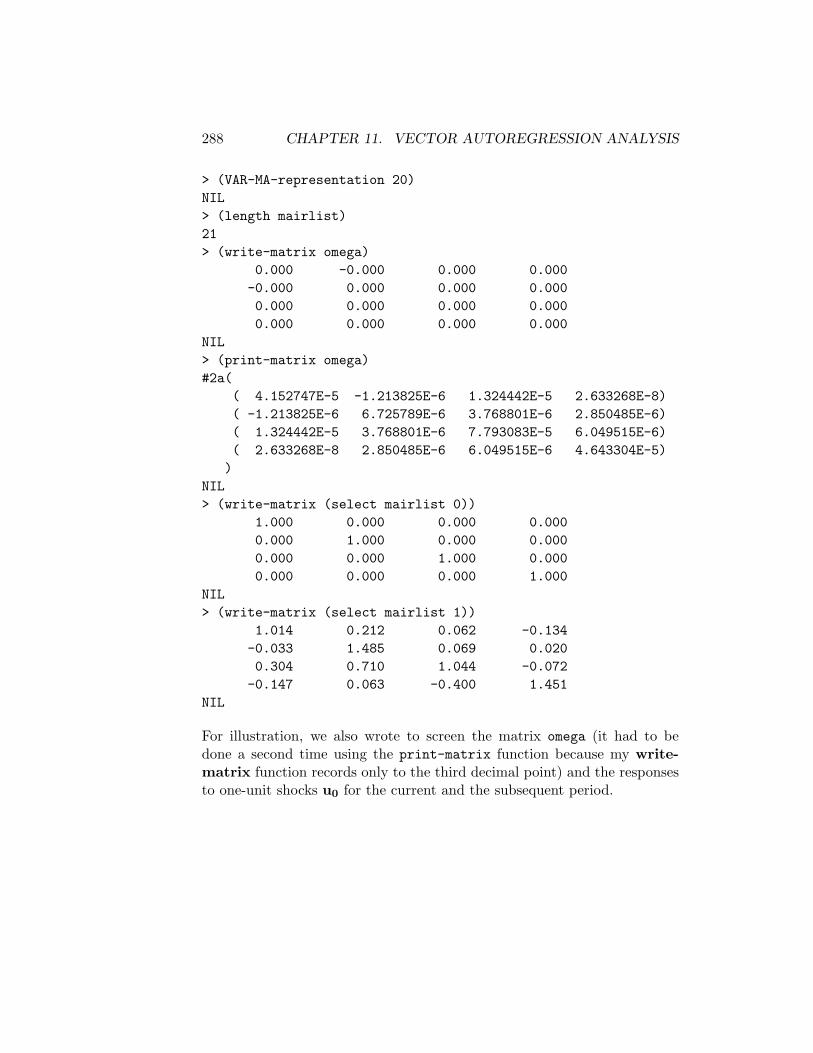
288 CHAPTER 11. VECTOR AUTOREGRESSION ANALYSIS
> (VAR-MA-representation 20)NIL> (length mairlist)21> (write-matrix omega)
0.000 -0.000 0.000 0.000-0.000 0.000 0.000 0.0000.000 0.000 0.000 0.0000.000 0.000 0.000 0.000
NIL> (print-matrix omega)#2a(
( 4.152747E-5 -1.213825E-6 1.324442E-5 2.633268E-8)( -1.213825E-6 6.725789E-6 3.768801E-6 2.850485E-6)( 1.324442E-5 3.768801E-6 7.793083E-5 6.049515E-6)( 2.633268E-8 2.850485E-6 6.049515E-6 4.643304E-5))
NIL> (write-matrix (select mairlist 0))
1.000 0.000 0.000 0.0000.000 1.000 0.000 0.0000.000 0.000 1.000 0.0000.000 0.000 0.000 1.000
NIL> (write-matrix (select mairlist 1))
1.014 0.212 0.062 -0.134-0.033 1.485 0.069 0.0200.304 0.710 1.044 -0.072
-0.147 0.063 -0.400 1.451NIL
For illustration, we also wrote to screen the matrix omega (it had to bedone a second time using the print-matrix function because my write-matrix function records only to the third decimal point) and the responsesto one-unit shocks u0 for the current and the subsequent period.

11.3. IDENTIFICATION 289
11.3 Identification
The moving average representation (11.11) does not give a proper indicationof how the system responds to shocks to the individual structural equations.The problem is that the shocks to the equations contained in the vector ut
are correlated with each other. We therefore cannot determine what theeffects on the m variables of a shock to an individual structural equationalone would be—an observed ut will represent the combined shocks to anumber of equations. This can be seen from the fact that from (11.9)
ut = (I−A0)−1 et.
In order to determine the effects of a shock to an individual structural equa-tion of the system we have to be able to solve the system for A0 and therebyobtain (I −A0)−1. This will enable us to operate on (11.11) to transformthe ut−j ’s in into et−j ’s. In the process, of course, the matrices Cj will alsobe transformed into a useful representation of the impulse-responses.
One way to obtain the matrix A0 is to statistically estimate the struc-tural model (11.4). Were we to do this, we would not be running a VAR.Indeed, the reason for VAR analysis is to avoid multi-equation structuralmodels.
The approach used to identify A0 in VAR analysis is to find the matrixthat will orthogonalize the errors—i.e., transform the ut−j series into theet−j series, the elements of which will be uncorrelated with each other.
Given any matrix G that has an inverse, equation (11.11) can be rewrit-ten
yt = C0 GG−1 ut + C1 GG−1 ut−1 + C2 GG−1 ut−2
+ · · · · · ·+ Cs GG−1 ut−s + y0. (11.16)
Our task is to find the G for which
G = (I−A0)−1.
Then
yt = Z0 et + Z1 et−1 + Z2 et−2
+ · · · · · ·+ Zs et−s + y0 (11.17)
whereZj = Cj G
andet−j = G−1 ut−j ==⇒ ut−j = Get−j

290 CHAPTER 11. VECTOR AUTOREGRESSION ANALYSIS
11.3.1 Choleski Decompositions
Suppose that the matrix A0 takes the following form:
0 0 0 · · · · · · · · · · · · 0 0a0
21 0 0 · · · · · · · · · · · · 0 0a0
31 a032 0 · · · · · · · · · · · · 0 0
a041 a0
42 a043 · · · · · · · · · · · · 0 0
......
......
......
......
......
......
......
......
......
......
......
......
......
...a0
m1 a0m2 a0
m3 · · · · · · · · · · · · a0m(m−1) 0
This will mean that the structural equations will take the form:
y1t = a111 y1(t−1) + a1
12 y2(t−1) · · · · · · · · · · · · · · · · · · · · · · · · · · · · · · · · · · · ·y2t = a0
21 y1t + a121 y1(t−1) + a1
22 y2(t−1) · · · · · · · · · · · · · · · · · · · · · · · · · · ·y3t = a0
31 y1t + a032 y2t + a1
31 y1(t−1) + a132 y2(t−1) · · · · · · · · · · · · · · · · · ·
y4t = a041 y1t + a0
42 y2t + a043 y3t + a1
41 y1(t−1) + a142 y2(t−1) · · · · · · · · ·
· · · = · · · · · · · · · · · · · · · · · · · · · · · · · · · · · · · · · · · · · · · · · · · · · · · · · · · · · · · · ·· · · = · · · · · · · · · · · · · · · · · · · · · · · · · · · · · · · · · · · · · · · · · · · · · · · · · · · · · · · · ·· · · = · · · · · · · · · · · · · · · · · · · · · · · · · · · · · · · · · · · · · · · · · · · · · · · · · · · · · · · · ·
None of the current year values of y2, y3, y4, · · · · · · · · · , ym enter into thedetermination of the current year level of y1. The current year level of y1
enters into the determination of the current year level of y2 and both thecurrent levels of y1 and y2 enter into the determination of the current levelof y3, the current levels of y1, y2 and y3 enter into the determination of thecurrent level of y4, and so forth. This system is a recursive system.
The standard approach to identifying the elements of A0 in VAR analysisis to decompose the matrix of reduced form residuals
ut u′t = Ω = Get(Get)′ = Gete′t G′ = GDG′.
If we choose implicit units of measurement for the variables for which thestandard deviations of the structural errors are unity, D = I, and our prob-lem is to choose the matrix G for which
GG′ = Ω.

11.3. IDENTIFICATION 291
This simply involves doing a Choleski Decomposition of the matrix Ω. Wethus obtain
(I− A0)−1 = G
and, hence,A0 = I−G−1
where A0 is a representation of A0 after scaling of the variables to renderD = I. Using the matrix G so obtained we can obtain the Zj matrices inequation (11.17) with the errors et having unit variance.
The upper-left-corner element of Z0 gives the response of y1 to a onestandard-deviation shock to the first equation in the current period. Thesum of the upper-left-corner elements of Z0 and Z1 gives the response ofy1 to a one standard-deviation shock to the first equation in the previousperiod. And sum of the of the upper-left-corner elements of Z0,Z1 and Z2
gives the response of that variable to a one standard-deviation shock to thefirst equation two periods previously, and so forth. The response of thefirst variable to a one-standard-deviation shock to the second variable in thecurrent and previous periods is given by the second elements from the leftin the top rows of the Zj matrices. And the response of the second variableto orthogonal one-standard-deviation shocks to the other variables is givenby the elements of the second rows of the Zj matrices, and so forth. Thesematrices are called impulse-response functions.
It is important to emphasize that this decomposition of Ω and theimpulse-response functions that are obtained from it are critically dependenton the ordering of the variables in the VAR. Had we ordered the variablesdifferently, putting the fourth variable first and the first variable fourth, forexample, the Choleski decomposition would have led to different impulse-response functions.4 Economic theory has to be used to decide which order-ing of the variables to use. In many cases, no such ordering is acceptablebecause the theoretical system that the VAR is being used to analyse is notrecursive.
The impulse responses for our United States VAR are calculated withthe following ordering as specified in the ordering of the variables in theobject varlist—the log of RGDP, the log of the implicit GDP deflator,the interest rate on 1-month commercial paper (measured as a fraction ofunity), and the logarithm of M1.
4This assumes that the error terms in the equations of the standard-form representationare correlated with each other so that the off-diagonal elements of Ω are non-zero. If theseoff-diagonal terms are zero, the impulse-response functions obtained from all the differentorderings will be the same.
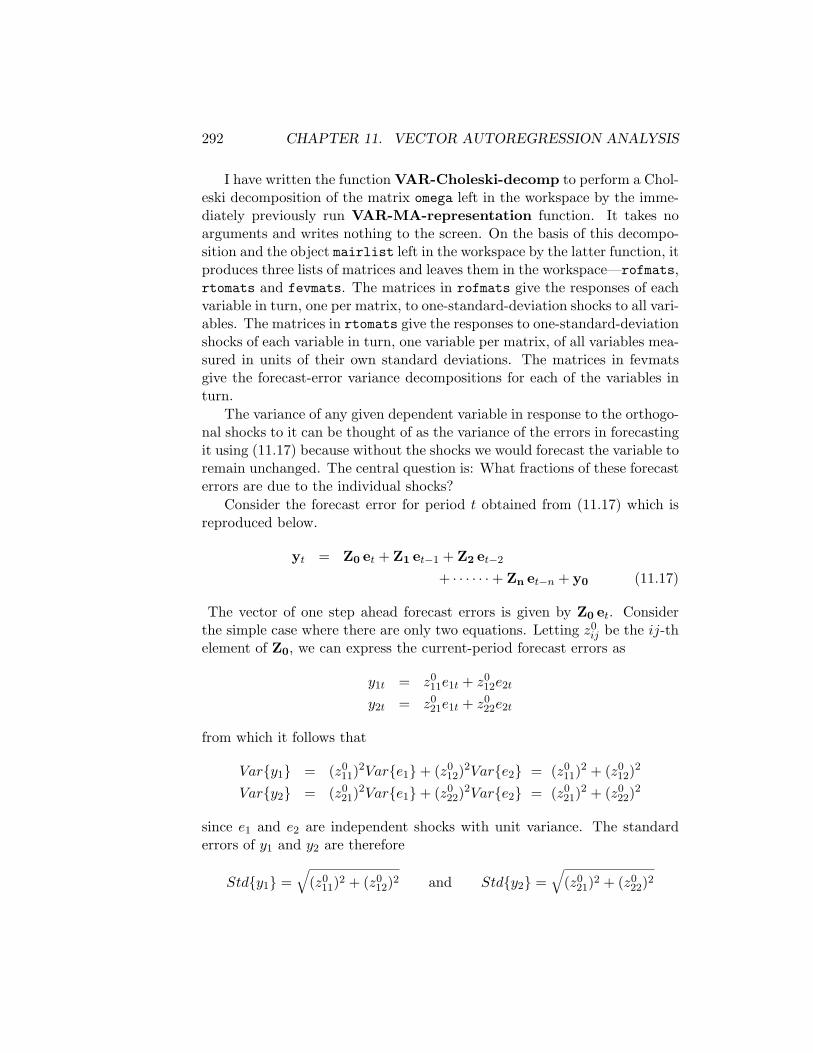
292 CHAPTER 11. VECTOR AUTOREGRESSION ANALYSIS
I have written the function VAR-Choleski-decomp to perform a Chol-eski decomposition of the matrix omega left in the workspace by the imme-diately previously run VAR-MA-representation function. It takes noarguments and writes nothing to the screen. On the basis of this decompo-sition and the object mairlist left in the workspace by the latter function, itproduces three lists of matrices and leaves them in the workspace—rofmats,rtomats and fevmats. The matrices in rofmats give the responses of eachvariable in turn, one per matrix, to one-standard-deviation shocks to all vari-ables. The matrices in rtomats give the responses to one-standard-deviationshocks of each variable in turn, one variable per matrix, of all variables mea-sured in units of their own standard deviations. The matrices in fevmatsgive the forecast-error variance decompositions for each of the variables inturn.
The variance of any given dependent variable in response to the orthogo-nal shocks to it can be thought of as the variance of the errors in forecastingit using (11.17) because without the shocks we would forecast the variable toremain unchanged. The central question is: What fractions of these forecasterrors are due to the individual shocks?
Consider the forecast error for period t obtained from (11.17) which isreproduced below.
yt = Z0 et + Z1 et−1 + Z2 et−2
+ · · · · · ·+ Zn et−n + y0 (11.17)
The vector of one step ahead forecast errors is given by Z0 et. Considerthe simple case where there are only two equations. Letting z0
ij be the ij-thelement of Z0, we can express the current-period forecast errors as
y1t = z011e1t + z0
12e2t
y2t = z021e1t + z0
22e2t
from which it follows that
Vary1 = (z011)
2Vare1+ (z012)
2Vare2 = (z011)
2 + (z012)
2
Vary2 = (z021)
2Vare1+ (z022)
2Vare2 = (z021)
2 + (z022)
2
since e1 and e2 are independent shocks with unit variance. The standarderrors of y1 and y2 are therefore
Stdy1 =√
(z011)2 + (z0
12)2 and Stdy2 =√
(z021)2 + (z0
22)2

11.3. IDENTIFICATION 293
and the fraction of the error variance attributable to the shock to the firstand second equations are, respectively,
(z011)
2
(z011)2 + (z0
12)2and
(z012)
2
(z011)2 + (z0
12)2.
Now consider the two step ahead forecast. In this case the forecast errorsin response to the two period’s shocks are
y1t = z011e1t + z0
12e2t + z111e1(t−1) + z1
12e2(t−1)
y2t = z021e1t + z0
22e2t + z121e1(t−1) + z1
22e2(t−1)
where z1ij is the ij-th element of Z1. The variances of the respective two-
period forecast errors are
(z011)
2 + (z012)
2 + (z111)
2 + (z112)
2
and(z0
21)2 + (z0
22)2 + (z0
21)2 + (z0
22)2
and the standard errors of the two-period forecasts are√
(z011)2 + (z0
12)2 + (z111)2 + (z1
12)2
and √(z0
21)2 + (z022)2 + (z0
21)2 + (z022)2.
The fraction of the two-step ahead forecast error variance of y1 attributableto the shock to the first shock is
(z011)
2 + (z111)
2
(z011)2 + (z0
12)2 + (z111)2 + (z1
12)2
and the fraction attributable to the second shock is
(z012)
2 + (z112)
2
(z011)2 + (z0
12)2 + (z111)2 + (z1
12)2
And the fractions of the two-step ahead forecast error variance of y2 at-tributable to the respective shocks are
(z021)
2 + (z121)
2
(z021)2 + (z0
22)2 + (z121)2 + (z1
22)2

294 CHAPTER 11. VECTOR AUTOREGRESSION ANALYSIS
and(z0
22)2 + (z1
22)2
(z021)2 + (z0
22)2 + (z121)2 + (z1
22)2.
The derivations of the forecast error variances and the fractions attributableto the two shocks for forecasts greater than two-steps ahead are straight-forward extensions of the calculations above.
As follow-ups to the VAR-Choleski-decomp function, I have writ-ten a number of functions to print the results to screen and plot them ongraphs. The function VAR-print-impulse-responses prints the matricesin rofmats and rtomats to the screen. To print the forecast-error-variance-decompositions to the screen, I wrote the function VAR-print-forecast-error-variance-decompositions and to print them to a LATEXfile I wrotethe function VAR-write-fev-decomps-to-LaTeX-file. The two functionsVAR-plot-impulse-responses-of and VAR-plot-impulse-responses-toplot rofmats and rtomats, respectively, to the screen. Each of these latterfunctions will send m2 plots to the screen, where m is the number of vari-ables, with each plot containing the response of a single variable to a shockto another variable. All these functions take as their single argument a listof strings giving the names of the variables—the varnames object requiredearlier can be used as the argument. The print-to-screen functions yield thefollowing results.
> (VAR-choleski-decomp)NIL> (VAR-print-impulse-responses varnames)
Responses of LOGRGDP to one-standard-deviation shocks to
Step LOGRGDP LOGIPD INTRATE LOGM10 0.00644418 0.00000000 0.00000000 0.000000001 0.00662420 0.00050002 0.00045479 -0.000895642 0.00655329 0.00034005 -0.00174511 -0.000778103 0.00518368 -0.00089579 -0.00312284 -0.002058564 0.00416718 -0.00173739 -0.00355574 -0.002564045 0.00327178 -0.00252315 -0.00500637 -0.003392576 0.00246164 -0.00307182 -0.00609400 -0.003909227 0.00172531 -0.00366446 -0.00641680 -0.004199858 0.00115625 -0.00397119 -0.00684735 -0.004513289 0.00077554 -0.00411592 -0.00720284 -0.0047247510 0.00049694 -0.00423856 -0.00719111 -0.00479430

11.3. IDENTIFICATION 295
11 0.00032502 -0.00422380 -0.00713198 -0.0048060312 0.00023368 -0.00411133 -0.00708591 -0.0047727013 0.00018060 -0.00398541 -0.00692205 -0.0046695114 0.00015516 -0.00382599 -0.00673150 -0.0045318915 0.00014850 -0.00363319 -0.00657588 -0.0043777416 0.00014366 -0.00344445 -0.00640549 -0.0042006217 0.00013547 -0.00326000 -0.00623229 -0.0040129818 0.00012477 -0.00307362 -0.00608561 -0.0038268519 0.00010901 -0.00289639 -0.00594815 -0.0036418720 0.00008837 -0.00272964 -0.00581354 -0.00346134
Responses of LOGIPD to one-standard-deviation shocks to
Step LOGRGDP LOGIPD INTRATE LOGM10 -0.00018836 0.00258656 0.00000000 0.000000001 -0.00035018 0.00397350 0.00058834 0.000131842 -0.00032374 0.00511017 0.00105526 0.000142483 -0.00002894 0.00654274 0.00133369 0.000338414 0.00019242 0.00773483 0.00170874 0.000601045 0.00036937 0.00878545 0.00201931 0.000850746 0.00053788 0.00973613 0.00218462 0.001036287 0.00068250 0.01053297 0.00232162 0.001186128 0.00080816 0.01119964 0.00241274 0.001285409 0.00092202 0.01177020 0.00242851 0.00131971
10 0.00102598 0.01223910 0.00241586 0.0012991211 0.00112547 0.01261918 0.00238617 0.0012243312 0.00122789 0.01293216 0.00232737 0.0010962213 0.00133464 0.01318393 0.00225410 0.0009237514 0.00144598 0.01338210 0.00217571 0.0007141515 0.00156280 0.01353770 0.00208712 0.0004719716 0.00168401 0.01365593 0.00199052 0.0002041817 0.00180763 0.01374031 0.00188962 -0.0000825118 0.00193203 0.01379565 0.00178214 -0.0003832719 0.00205530 0.01382482 0.00166721 -0.0006932420 0.00217540 0.01382931 0.00154589 -0.00100783
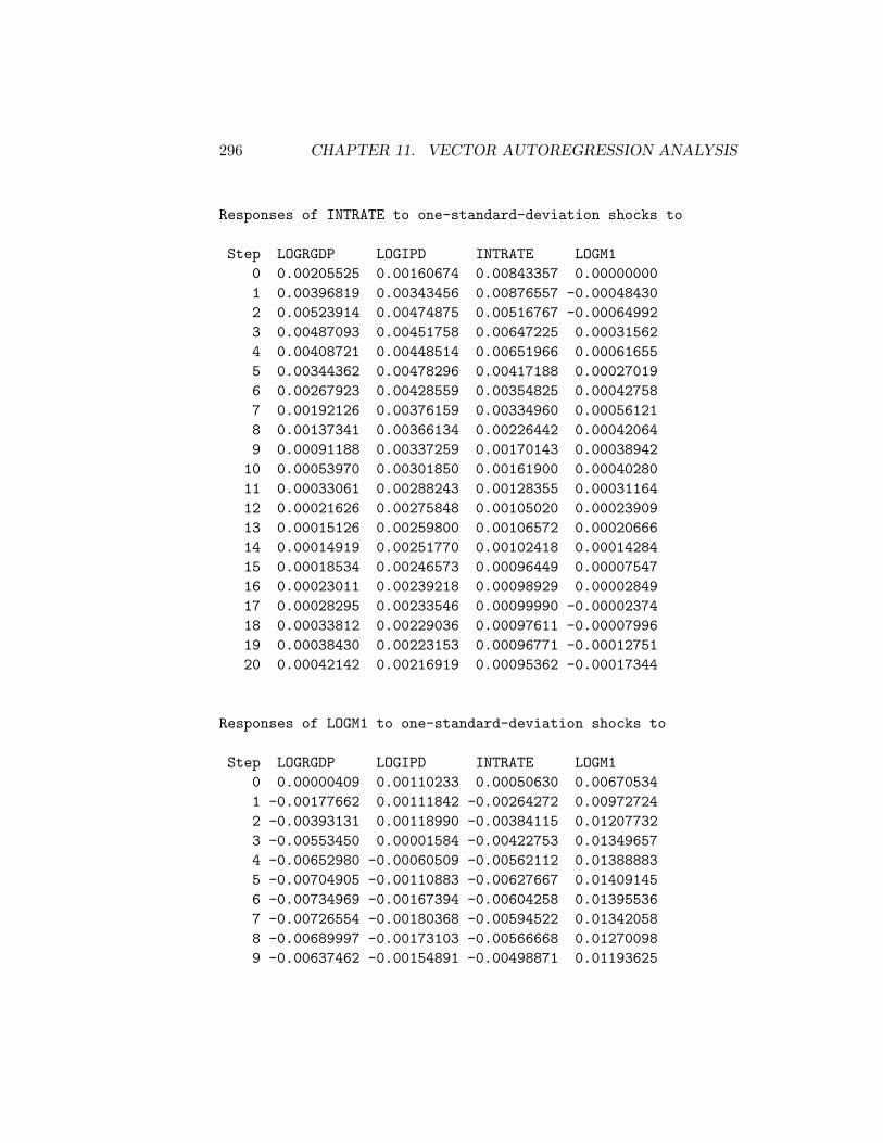
296 CHAPTER 11. VECTOR AUTOREGRESSION ANALYSIS
Responses of INTRATE to one-standard-deviation shocks to
Step LOGRGDP LOGIPD INTRATE LOGM10 0.00205525 0.00160674 0.00843357 0.000000001 0.00396819 0.00343456 0.00876557 -0.000484302 0.00523914 0.00474875 0.00516767 -0.000649923 0.00487093 0.00451758 0.00647225 0.000315624 0.00408721 0.00448514 0.00651966 0.000616555 0.00344362 0.00478296 0.00417188 0.000270196 0.00267923 0.00428559 0.00354825 0.000427587 0.00192126 0.00376159 0.00334960 0.000561218 0.00137341 0.00366134 0.00226442 0.000420649 0.00091188 0.00337259 0.00170143 0.0003894210 0.00053970 0.00301850 0.00161900 0.0004028011 0.00033061 0.00288243 0.00128355 0.0003116412 0.00021626 0.00275848 0.00105020 0.0002390913 0.00015126 0.00259800 0.00106572 0.0002066614 0.00014919 0.00251770 0.00102418 0.0001428415 0.00018534 0.00246573 0.00096449 0.0000754716 0.00023011 0.00239218 0.00098929 0.0000284917 0.00028295 0.00233546 0.00099990 -0.0000237418 0.00033812 0.00229036 0.00097611 -0.0000799619 0.00038430 0.00223153 0.00096771 -0.0001275120 0.00042142 0.00216919 0.00095362 -0.00017344
Responses of LOGM1 to one-standard-deviation shocks to
Step LOGRGDP LOGIPD INTRATE LOGM10 0.00000409 0.00110233 0.00050630 0.006705341 -0.00177662 0.00111842 -0.00264272 0.009727242 -0.00393131 0.00118990 -0.00384115 0.012077323 -0.00553450 0.00001584 -0.00422753 0.013496574 -0.00652980 -0.00060509 -0.00562112 0.013888835 -0.00704905 -0.00110883 -0.00627667 0.014091456 -0.00734969 -0.00167394 -0.00604258 0.013955367 -0.00726554 -0.00180368 -0.00594522 0.013420588 -0.00689997 -0.00173103 -0.00566668 0.012700989 -0.00637462 -0.00154891 -0.00498871 0.01193625
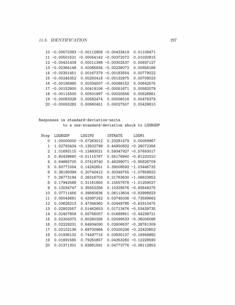
11.3. IDENTIFICATION 297
10 -0.00572383 -0.00112858 -0.00433419 0.0110847111 -0.00501521 -0.00054142 -0.00372072 0.0102081512 -0.00431409 0.00011398 -0.00302537 0.0093712713 -0.00364148 0.00085934 -0.00238072 0.0085616614 -0.00301451 0.00167379 -0.00183554 0.0077902215 -0.00245352 0.00250418 -0.00132875 0.0070802316 -0.00195985 0.00334507 -0.00088152 0.0064257517 -0.00152800 0.00419106 -0.00051671 0.0058207918 -0.00115500 0.00501997 -0.00020556 0.0052686119 -0.00083328 0.00582474 0.00006016 0.0047637920 -0.00055282 0.00660451 0.00027507 0.00429810
Responses in standard-deviation-unitsto a one-standard-deviation shock to LOGRGDP
Step LOGRGDP LOGIPD INTRATE LOGM10 1.00000000 -0.07263012 0.23281479 0.000599671 1.02793434 -0.13502799 0.44950832 -0.260723562 1.01693115 -0.12483021 0.59347927 -0.576930173 0.80439660 -0.01115767 0.55176940 -0.812203104 0.64665700 0.07419740 0.46299071 -0.958267095 0.50771054 0.14242651 0.39008592 -1.034467326 0.38199399 0.20740412 0.30349755 -1.078588227 0.26773194 0.26316703 0.21763630 -1.066238528 0.17942568 0.31161855 0.15557678 -1.012590279 0.12034747 0.35552256 0.10329576 -0.93549275
10 0.07711456 0.39560836 0.06113604 -0.8399882311 0.05043681 0.43397242 0.03745036 -0.7359966212 0.03626213 0.47346360 0.02449785 -0.6331047513 0.02802557 0.51462653 0.01713476 -0.5343973514 0.02407809 0.55756057 0.01689951 -0.4423872115 0.02304375 0.60260256 0.02099533 -0.3600608616 0.02229231 0.64934090 0.02606637 -0.2876130917 0.02102136 0.69700984 0.03205238 -0.2242385218 0.01936132 0.74497715 0.03830137 -0.1694988219 0.01691565 0.79250857 0.04353260 -0.1222859020 0.01371301 0.83881591 0.04773776 -0.08112853

298 CHAPTER 11. VECTOR AUTOREGRESSION ANALYSIS
Responses in standard-deviation-unitsto a one-standard-deviation shock to LOGIPD
Step LOGRGDP LOGIPD INTRATE LOGM10 0.00000000 0.99735894 0.18200792 0.161770491 0.07759171 1.53214974 0.38905948 0.164131452 0.05276918 1.97044392 0.53792901 0.174621553 -0.13900833 2.52282916 0.51174176 0.002324274 -0.26960582 2.98249225 0.50806787 -0.088798225 -0.39153924 3.38760314 0.54180346 -0.162723516 -0.47668149 3.75417661 0.48546263 -0.245656017 -0.56864574 4.06143062 0.42610528 -0.264695168 -0.61624357 4.31849446 0.41474951 -0.254033129 -0.63870331 4.53849923 0.38203970 -0.2273065910 -0.65773438 4.71930283 0.34192933 -0.1656226811 -0.65544381 4.86586018 0.32651558 -0.0794551412 -0.63799168 4.98654308 0.31247539 0.0167261813 -0.61845038 5.08362377 0.29429573 0.1261107814 -0.59371164 5.16003396 0.28519968 0.2456339715 -0.56379409 5.22003409 0.27931300 0.3674948716 -0.53450585 5.26562125 0.27098140 0.4908989917 -0.50588272 5.29815656 0.26455662 0.6150502618 -0.47695990 5.31949679 0.25944683 0.7366942219 -0.44945755 5.33074473 0.25278278 0.8547976420 -0.42358217 5.33247517 0.24572141 0.96923054
Responses in standard-deviation-unitsto a one-standard-deviation shock to INTRATE
Step LOGRGDP LOGIPD INTRATE LOGM10 0.00000000 0.00000000 0.95533784 0.074301631 0.07057410 0.22686046 0.99294609 -0.387826132 -0.27080324 0.40689915 0.58538334 -0.563699803 -0.48459865 0.51426015 0.73316372 -0.620402284 -0.55177493 0.65887513 0.73853383 -0.824914485 -0.77688195 0.77863175 0.47258237 -0.921118736 -0.94565892 0.84237088 0.40193850 -0.886765657 -0.99575040 0.89519827 0.37943587 -0.87247706
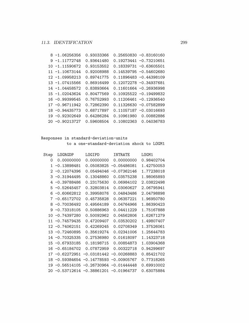
11.3. IDENTIFICATION 299
8 -1.06256356 0.93033366 0.25650830 -0.831601609 -1.11772748 0.93641480 0.19273441 -0.73210651
10 -1.11590672 0.93153552 0.18339731 -0.6360550111 -1.10673144 0.92008988 0.14539795 -0.5460268012 -1.09958213 0.89741775 0.11896483 -0.4439810913 -1.07415566 0.86916499 0.12072278 -0.3493768114 -1.04458572 0.83893664 0.11601664 -0.2693699815 -1.02043624 0.80477569 0.10925522 -0.1949983216 -0.99399545 0.76752993 0.11206461 -0.1293654017 -0.96711942 0.72862390 0.11326630 -0.0758289918 -0.94435773 0.68717897 0.11057187 -0.0301669319 -0.92302649 0.64286284 0.10961980 0.0088288620 -0.90213727 0.59608504 0.10802363 0.04036783
Responses in standard-deviation-unitsto a one-standard-deviation shock to LOGM1
Step LOGRGDP LOGIPD INTRATE LOGM10 0.00000000 0.00000000 0.00000000 0.984027041 -0.13898481 0.05083825 -0.05486081 1.427500532 -0.12074396 0.05494046 -0.07362146 1.772380183 -0.31944495 0.13048860 0.03575238 1.980658934 -0.39788486 0.23175630 0.06984102 2.038224985 -0.52645457 0.32803814 0.03060627 2.067959416 -0.60662812 0.39958076 0.04843486 2.047988987 -0.65172702 0.45735828 0.06357221 1.969507808 -0.70036492 0.49564189 0.04764966 1.863904239 -0.73318105 0.50886963 0.04411229 1.75167888
10 -0.74397280 0.50092962 0.04562806 1.6267127911 -0.74579435 0.47209407 0.03530202 1.4980740712 -0.74062151 0.42269245 0.02708349 1.3752606113 -0.72460895 0.35619274 0.02341006 1.2564478314 -0.70325335 0.27536980 0.01618097 1.1432371815 -0.67933185 0.18198715 0.00854873 1.0390436816 -0.65184702 0.07872959 0.00322718 0.9429969717 -0.62272951 -0.03181442 -0.00268883 0.8542170218 -0.59384654 -0.14778593 -0.00905767 0.7731826519 -0.56514105 -0.26730964 -0.01444448 0.6991000220 -0.53712614 -0.38861201 -0.01964737 0.63075884

300 CHAPTER 11. VECTOR AUTOREGRESSION ANALYSIS
NIL> (VAR-print-forecast-error-variance-decompositions varnames)
Forecast-Error-Variance-Decomposition of LOGRGDP
Step LOGRGDP LOGIPD INTRATE LOGM10 100.00000000 0.00000000 0.00000000 0.000000001 98.54727191 0.28847958 0.23865752 0.925591002 96.23215905 0.27414602 2.43834480 1.055350133 88.67824158 0.66732843 7.42931413 3.225115864 80.40751143 1.95050623 11.94898908 5.692993255 68.31995409 3.93344169 18.90192075 8.844683486 56.32132964 5.94554228 26.12962656 11.603501537 46.74776317 8.12240755 31.36049272 13.769336568 39.06276177 9.92117548 35.48114942 15.534913339 33.06524174 11.25531586 38.77088821 16.9085542010 28.58668990 12.35873774 41.07676801 17.9778043511 25.19856281 13.19795195 42.77441918 18.8290660612 22.57642156 13.78150908 44.13544052 19.5066288513 20.54032704 14.21209290 45.20295942 20.0446206414 18.93463538 14.52280790 46.07015911 20.4723976115 17.63961199 14.72357771 46.83096135 20.8058489416 16.58175491 14.84916958 47.51084741 21.0582281017 15.70627926 14.92075457 48.12996292 21.2430032418 14.96954646 14.94567003 48.71450002 21.3702834919 14.34179525 14.93561022 49.27334940 21.4492451320 13.80148315 14.90016893 49.80929340 21.48905452
Forecast-Error-Variance-Decomposition of LOGIPD
Step LOGRGDP LOGIPD INTRATE LOGM10 0.52751349 99.47248651 0.00000000 0.000000001 0.68740653 97.73207005 1.50494725 0.075576162 0.52213773 96.50406807 2.89895390 0.074840313 0.27747217 96.15547799 3.40692479 0.160125054 0.19012436 95.59264654 3.89266911 0.324559995 0.18192737 95.04404581 4.25921387 0.514812956 0.21290292 94.71179918 4.39805828 0.67723963

11.3. IDENTIFICATION 301
7 0.25951090 94.49161959 4.43966083 0.809208688 0.31119868 94.36181278 4.42140864 0.905579909 0.36424548 94.33482146 4.33992598 0.96100707
10 0.41720128 94.37882999 4.22451392 0.9794548011 0.47038693 94.46956946 4.09405660 0.9659870212 0.52538578 94.59623069 3.95205327 0.9263302613 0.58353828 94.74338202 3.80495398 0.8681257114 0.64586266 94.89651333 3.65836181 0.7992622015 0.71327971 95.04599825 3.51359136 0.7271306816 0.78638110 95.18335231 3.37157541 0.6586911917 0.86538084 95.30115435 3.23334128 0.6001235318 0.95023617 95.39414060 3.09898564 0.5566375819 1.04065382 95.45849169 2.96839602 0.5324584720 1.13610477 95.49144161 2.84164499 0.53080863
Forecast-Error-Variance-Decomposition of INTRATE
Step LOGRGDP LOGIPD INTRATE LOGM10 5.42027252 3.31268819 91.26703930 0.000000001 10.94019004 7.87636609 81.05495437 0.128489502 18.26134257 14.22130426 67.26436138 0.252991793 20.57444357 16.58123863 62.62552945 0.218788364 20.64631724 18.20284256 60.88370028 0.267139925 20.87207637 21.00209886 57.87260109 0.253223686 20.71329240 23.00174184 56.01511678 0.269848977 20.27446248 24.35718115 55.05529534 0.313061038 19.86995618 25.83928816 53.95782506 0.332930599 19.49161766 27.11811083 53.03998794 0.35028358
10 19.14044993 28.09659076 52.39252887 0.3704304511 18.83630836 29.00001813 51.78338966 0.3802838512 18.57278746 29.82503342 51.21803562 0.3841435013 18.33843917 30.53077430 50.74468203 0.3861045014 18.12493824 31.17910672 50.31117022 0.3847848215 17.92906949 31.79053540 49.89898627 0.3814088316 17.74856096 32.34774326 49.52617601 0.3775197717 17.58196584 32.86314409 49.18108967 0.3738004018 17.42966915 33.34736365 48.85179916 0.3711680419 17.29159181 33.79429320 48.54390188 0.3702131120 17.16715560 34.20513951 48.25621211 0.37149279
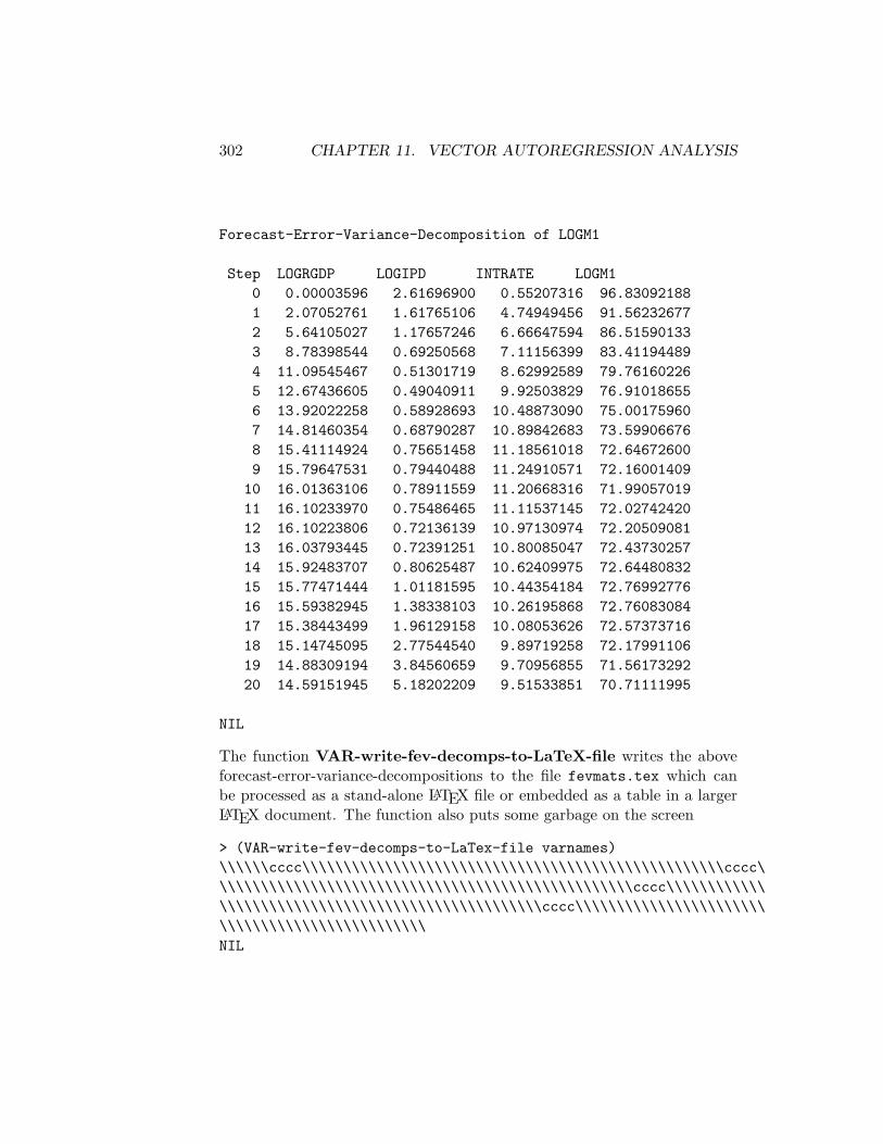
302 CHAPTER 11. VECTOR AUTOREGRESSION ANALYSIS
Forecast-Error-Variance-Decomposition of LOGM1
Step LOGRGDP LOGIPD INTRATE LOGM10 0.00003596 2.61696900 0.55207316 96.830921881 2.07052761 1.61765106 4.74949456 91.562326772 5.64105027 1.17657246 6.66647594 86.515901333 8.78398544 0.69250568 7.11156399 83.411944894 11.09545467 0.51301719 8.62992589 79.761602265 12.67436605 0.49040911 9.92503829 76.910186556 13.92022258 0.58928693 10.48873090 75.001759607 14.81460354 0.68790287 10.89842683 73.599066768 15.41114924 0.75651458 11.18561018 72.646726009 15.79647531 0.79440488 11.24910571 72.1600140910 16.01363106 0.78911559 11.20668316 71.9905701911 16.10233970 0.75486465 11.11537145 72.0274242012 16.10223806 0.72136139 10.97130974 72.2050908113 16.03793445 0.72391251 10.80085047 72.4373025714 15.92483707 0.80625487 10.62409975 72.6448083215 15.77471444 1.01181595 10.44354184 72.7699277616 15.59382945 1.38338103 10.26195868 72.7608308417 15.38443499 1.96129158 10.08053626 72.5737371618 15.14745095 2.77544540 9.89719258 72.1799110619 14.88309194 3.84560659 9.70956855 71.5617329220 14.59151945 5.18202209 9.51533851 70.71111995
NIL
The function VAR-write-fev-decomps-to-LaTeX-file writes the aboveforecast-error-variance-decompositions to the file fevmats.tex which canbe processed as a stand-alone LATEX file or embedded as a table in a largerLATEX document. The function also puts some garbage on the screen
> (VAR-write-fev-decomps-to-LaTex-file varnames)\\\\\\cccc\\\\\\\\\\\\\\\\\\\\\\\\\\\\\\\\\\\\\\\\\\\\\\\\\\\cccc\\\\\\\\\\\\\\\\\\\\\\\\\\\\\\\\\\\\\\\\\\\\\\\\\\\cccc\\\\\\\\\\\\\\\\\\\\\\\\\\\\\\\\\\\\\\\\\\\\\\\\\\\cccc\\\\\\\\\\\\\\\\\\\\\\\\\\\\\\\\\\\\\\\\\\\\\\\\NIL

11.3. IDENTIFICATION 303
The impulse-responses are shown in Figure 17 with the responses mea-sured in standard-deviation units of the responding variable. Note that thevertical scale on the upper right panel is greater than the common verticalscale on the remaining panels. The shocks are one unit shocks, equal to onestandard deviation of the relevant component of the vector et. These resultsmight give superficial encouragement to those that interpret U.S. monetarypolicy as operating through changes in the level at which the Federal Re-serve sets short-term interest rates. An upward shock to the interest rateon 1-month commercial paper the lower-left panel is associated with a sub-sequent negative response of both M1, over which the Fed has some control,and real GDP. While the Fed operates on the federal funds rate and not oncommercial paper rates, those two interest rates move very closely together.The argument would be that the Fed announces a tighter policy, causingshort-term rates to rise and then validates that announcement with a subse-quent decline in M1, resulting in a decline in real GDP. There are, however,some obvious difficulties with this interpretation. First, as can also be seenin the lower-left panel, the price level subsequently increases in response tothe positive shock to short-term interest rates at a time when real GDP isfalling. Furthermore, as is evident in the lower-right panel a positive shockto M1, while causing the price level to rise, leads to a subsequent fall in realGDP.
The crucial assumption underlying the results in Table 17 is that themodel is assumed to be recursive, with real GDP being unaffected by shocksto all the other variables in the current quarter, the implicit GDP deflatorbeing affected only by current-quarter real GDP shocks, along with shocksto itself, the interest rate being affected only by current-quarter shocks toreal GDP, the GDP deflator and itself, and the M1 variable being affected bycurrent-quarter shocks to itself and to all the other variables. This impliesthat the Fed, in setting monetary policy, pays attention to observed levelsof all of the other variables during the current quarter but its policies haveno current-quarter effects on any of those other variables. An alternativeassumption would be to order the variables in exactly the opposite fashion,with M1 shocks unaffected by current-quarter shocks to any of the the othervariables, interest rate shocks being affected by current-quarter shocks to it-self and to M1, price level being affected by current-quarter shocks to itself,interest rates and base money, and real GDP being affected by current-quarter shocks to all the variables, including itself. This ordering wouldhave the Fed basing its current policy only on what is observed in previousquarters but not on what is happening in the current quarter. Its inabilityto use within-quarter information about the other variables could be inter-

304 CHAPTER 11. VECTOR AUTOREGRESSION ANALYSIS
-1
-0.5
0
0.5
1
1.5
2
2.5
0 5 10 15 20
Response to RGDP Shock
RGDPIPD
INTRM1
-1
0
1
2
3
4
5
6
0 5 10 15 20
Response to Price Level Shock
RGDPIPD
INTRM1
-1
-0.5
0
0.5
1
1.5
2
2.5
0 5 10 15 20
Response to Interest Rate Shock
RGDPIPD
INTRM1
-1
-0.5
0
0.5
1
1.5
2
2.5
0 5 10 15 20
Response to M1
RGDPIPD
INTRM1
Figure 17: The responses of the four variables to first period shocks of each.These responses are measured in standard-deviation units of the respondingvariable. The decomposition of Choleski with the variables ordered left-to-right, top-to-bottom.

11.3. IDENTIFICATION 305
-1
-0.5
0
0.5
1
1.5
2
2.5
0 5 10 15 20
Response to M1 Shock
M1INTR
IPDRGDP
-1
-0.5
0
0.5
1
1.5
2
2.5
0 5 10 15 20
Response to Interest Rate Shock
M1INTR
IPDRGDP
-1
0
1
2
3
4
5
6
0 5 10 15 20
Response to Price Level Shock
M1INTR
IPDRGDP
-1
-0.5
0
0.5
1
1.5
2
2.5
0 5 10 15 20
Response to RGDP Shock
M1INTR
IPDRGDP
Figure 18: The responses of the four variables to first period shocks of each.These responses are measured in standard-deviation units of the respondingvariable. The decomposition is Choleski with the variables ordered left-to-right, top-to-bottom.

306 CHAPTER 11. VECTOR AUTOREGRESSION ANALYSIS
preted as resulting from the lag in the availability of statistics measuringthe levels of those variables.
Figure 18 plots the impulse-responses that arise when we use the reverseordering of the variables to that in Figure 17 in the Choleski decomposition.The results are hardly distinguishable from those in Figure 17 althoughit appears that a positive shock to the interest rate now has a strongerpositive effect on real GDP in the current quarter and the one that followsas compared to that in Figure 17.
It turns out that the impulse-responses will be identical for the twoorderings of the variables if the off-diagonal terms in the matrix Ω are zero.In fact, we have previously printed out that matrix for the initial orderingof variables and, for convenience, reproduce that print-out here.
RGDP IPD INTR M1RGDP 4.152747E-5 -1.213825E-6 1.324442E-5 2.633268E-8IPD -1.213825E-6 6.725789E-6 3.768801E-6 2.850485E-6INTR 1.324442E-5 3.768801E-6 7.793083E-5 6.049515E-6M1 2.633268E-8 2.850485E-6 6.049515E-6 4.643304E-5
It is interesting that the only off-diagonal element that exceeds in magnitudeany of the diagonal elements is the covariance of the log real GDP residualswith those of the interest rate. But this covariance still falls short of thevariances of the residuals of either of these variables.
11.3.2 Structural Decompositions
The problem with the above analyses is that the system we are trying tomodel may not be recursive, making a Choleski decomposition inappropri-ate. Sims5 and Bernanke6 model the innovations using economic analysisthat postulates non-recursive relationships between the variables.
As in the Choleski decomposition, the object is to extract the coefficientsof G from the variance-covariation matrix of the reduced-form system Ω.The latter matrix is symmetric with the variances of the shocks along thediagonal and the covariances in the off-diagonal elements. It thus containsonly (m2 + m)/2 distinct elements, m being the number of variables. Weare therefore able to identify the same number of elements of (I − A0)−1
in G. This is precisely the number of elements identified by the Choleski5“Christopher Sims, “Are Forecasting Models Usable for Policy Analysis?” Federal
Reserve Bank of Minneapolis Quarterly Review (Winter 1986), 3–16.6Ben Bernanke, “Alternative Explanations of Money-Income Correlation,” Carnegie-
Rochester Conference Series on Public Policy 25 (1986), 49–100.
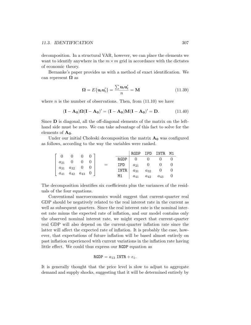
11.3. IDENTIFICATION 307
decomposition. In a structural VAR, however, we can place the elements wewant to identify anywhere in the m×m grid in accordance with the dictatesof economic theory.
Bernanke’s paper provides us with a method of exact identification. Wecan represent Ω as
Ω = Eutu′t =∑
utu′tn
= M (11.39)
where n is the number of observations. Then, from (11.10) we have
(I−A0)Ω(I−A0)′ = (I−A0)M(I−A0)′ = D. (11.40)
Since D is diagonal, all the off-diagonal elements of the matrix on the left-hand side must be zero. We can take advantage of this fact to solve for theelements of A0.
Under our initial Choleski decomposition the matrix A0 was configuredas follows, according to the way the variables were ranked.
0 0 0 0a21 0 0 0a31 a32 0 0a41 a42 a43 0
=
RGDP IPD INTR M1RGDP 0 0 0 0IPD a21 0 0 0INTR a31 a32 0 0M1 a41 a42 a43 0
The decomposition identifies six coefficients plus the variances of the resid-uals of the four equations.
Conventional macroeconomics would suggest that current-quarter realGDP should be negatively related to the real interest rate in the current aswell as subsequent quarters. Since the real interest rate is the nominal inter-est rate minus the expected rate of inflation, and our model contains onlythe observed nominal interest rate, we might expect that current-quarterreal GDP will also depend on the current-quarter inflation rate since thelatter will affect the expected rate of inflation. It is probably the case, how-ever, that expectations of future inflation will be based almost entirely onpast inflation experienced with current variations in the inflation rate havinglittle effect. We could thus express our RGDP equation as
RGDP = a13 INTR + ε1.
It is generally thought that the price level is slow to adjust to aggregatedemand and supply shocks, suggesting that it will be determined entirely by

308 CHAPTER 11. VECTOR AUTOREGRESSION ANALYSIS
what has happened in past quarters. Given the fact that prices in differentindustries adjust differently and at different times, there will be current-period random shocks to the price level.
IPD = ε2
The current-quarter interest rate will depend on that quarter’s demand forand supply of money. The quantity of money demanded depends on currentoutput (the volume of transactions), current inflation (which represents anaddition to the nominal volume of transactions) and the cost of holdingmoney, represented by the rate of interest. The supply of money dependson the quantity of base money supplied by the authorities together with amoney multiplier (ratio of M1 to base money) that will depend on all of ourother variables. The equation determining the interest rate will thus be ofthe form
INTR = a31 RGDP + a32 IPD + a33 INTR + a34 M1 + ε3.
The price level is relevant here because it affects the real stock of money.Finally, the authorities will try to set the stock of base money at a levelthat will produce output and price level stability around full-employmentlevels. In doing so, they will pay attention to the current inflation rate,the current interest rate, and the current deviation of output from its full-employment level. They will be able to observe current interest rate levelson a day-by-day basis and can estimate the inflation rate and price levelon a monthly basis. The current levels of the interest rate and prices willtherefore certainly be in their response function. Given the fact that outputgrowth can really only be estimated on a quarter-by-quarter basis, it wouldnot seem unreasonable to imagine that the authorities base their monetarypolicy on past levels of output rather than current levels that are impreciselymeasured. Under the assumption that M1 is indirectly controlled by theauthorities as a result of their monetary policy, the money equation willthen be
M1 = a42 IPD + a43 INTR + ε4
This implies the following A0 matrix.
RGDP IPD INTR M1RGDP 0 0 a13 0IPD 0 0 0 0INTR a31 a32 0 a34
M1 0 a42 a43 0

11.3. IDENTIFICATION 309
One might be tempted to add parameters to the above matrix, but thatwould result in the system being under-determined—all but six non-diagonalentries must be zero restrictions or we will not be able to solve the system.Imposing more zero restrictions would make the system over-identified. Asit stands, the system is just-identified with six aij ’s to be solved for.
Letting sij be the ij-th element of M in equation (11.40) and expanding(I−A0)M (I−A0)′, we obtain
1 0 −a13 00 1 0 0
−a31 −a32 1 −a34
0 −a42 −a43 1
s11 s21 s31 s41
s21 s22 s32 s42
s31 s32 s33 s43
s41 a42 s43 s44
1 0 −a31 −a41
0 1 −a32 −a42
−a13 0 1 00 0 −a34 1
=
g11 g12 g13 g14
g21 g22 g23 g24
g31 g32 g33 g34
g41 g42 g43 g44
1 0 −a31 00 1 −a32 −a42
−a13 0 1 −a43
0 0 −a34 1
where
g11 = s11 − a13s31
g12 = s21 − a13s32
g13 = s31 − a13s33
g14 = s41 − a13s43
g21 = s21
g22 = s22
g23 = s32
g24 = s42
g31 = −a31s11 − a32s21 + s31 − a34s41
g32 = −a31s21 − a32s22 + s32 − a34s42
g33 = −a31s31 − a32s32 + s33 − a34s43
g34 = −a31s41 − a32s42 + s43 − a34s44
g41 = −a42s21 − a43s31 + s41
g42 = −a42s22 − a43s32 + s42
g43 = −a42s32 − a43s33 + s43
g44 = −a42s42 − a43s43 + s44

310 CHAPTER 11. VECTOR AUTOREGRESSION ANALYSIS
Multiplying together the above two matrices, we then obtain
D =
d11 d12 d13 d14
d21 d22 d23 d24
d31 d32 d33 d34
d41 d42 d43 d44
where
d11 = g11 − g13a13
= s11 − a31s31 − a13s31 + a213s33 (11.41)
d22 = g22 = s22 (11.42)d33 = − a31g31 − a32g32 + g33 − g34a34
= a231s11 + a31a32s21 − a31s31 + a31a34s41
+ a32a31s21 + a232s22 − a32s32 + a32a34s42
− a31s31 − a32s32 + s33 − a34s43 + a34a31s41
+ a34a32s42 − a34s43 + a234s44 (11.43)
d44 = − a42g42 − a43g43 + g44
= + a242s22 + a42a43s32 − a42s42 + a43a42s32 + a2
43s33
− a42s42 − a43s43 + s44 (11.44)d12 = d21 = g12
= s21 − a13s32 = 0 (11.45)d13 = d31 = − a31g11 − a32g12 + g13 − a34g14
= − a31s11 + a31a13s31 − a32s21 + a32a13s32
+ s31 − a13s33 − a34s41 + a34a13s43 = 0 (11.46)d14 = d41 = −a42g12 − a43g13 + g14
= − a42s21 + a42a13s32 − a43s31 + a43a13s33
+ s41 − a13s43 = 0 (11.47)d23 = d32 = − a31g21 − a32g22 + g23 − a34g24
= −a31s21 − a32s22 + s32 − a34s42 = 0 (11.48)d24 = d42 = − a42g22 − a43g23 + g24
= − a42s22 − a43s32 + s42 = 0 (11.49)d34 = d43 = − a31g41 − a32g42 + g43 − a34g44
= a42a31s21 + a42a32s22 − a42s32 + a42a34s42 + a43a31s31
+ a43a32s32 − a43s33 + a43a34s43 − a31s41
− a32s42 + s43 − a34s44 = 0 (11.50)

11.3. IDENTIFICATION 311
The last six of these equations, (11.45) through (11.50) can be solved fora13, a31, a32, a34, a42 and a43. This gives us an estimate of the matrix A0
and, by matrix substitution, I −A0. These solutions for the aij can thenbe plugged into equations (11.41) through (11.44) to obtain the diagonalelements d11, d22, d33 and d44 and, hence, the matrix D.
Calculation of (I−A0) by itself is insufficient to obtain the matrix Gand the impulse-response functions. The matrix (I−A0) has to be scaled toreduce D to an identity matrix to ensure that the orthogonalized residualshave unit variance. Thus,
G = (I−A0)−1 D1/2
= (I− A0)−1 (11.51)
where A0 is the representation of A0 for which the et have unit variance.The task now at hand is to solve the above equations for the matrices
A0 and D. First, note from (11.45) that
a13 =s21
s32.
This value of a13 enables us to identify the magnitudes of g11, g12, g13 andg14. Equations (11.47) and (11.49) form the following two-equation systemin a42 and a43,
g12 a42 + g13 a43 = g14 (11.52)s22 a42 + s32 a43 = s42 (11.53)
When this system is solved for a41 and a42 we can then obtain the mag-nitudes of g41, g42, g43 and g44 which, when substituted along with theearlier-determined gij into (11.46) and (11.50) form with equation (11.48)the following three-equation system in a31, a32 and a33.
g11 a31 + g12 a32 + g14 a34 = g13 (11.54)s21 a31 + s22 a32 + s42 a34 = s32 (11.55)g41 a31 + g42 a32 + g44 a34 = g43 (11.56)
Once this system is solved, the solutions for d11, d22, d33 and d44 can beobtained by substitution.
To perform the structural-decomposition we have to write a functionthat makes the above calculations. Since each individual problem will re-quire a unique function, there is no point in copying our function to the

312 CHAPTER 11. VECTOR AUTOREGRESSION ANALYSIS
file addfuncs.lsp. Rather, we copy it to a separate file strucdec.lsp sothat it can be used as a template for calculating future functions to performother just-identified structural-decompositions. Of course, our function hasto be included a the batch file that contains the code for the particular VARanalysis we are performing. For the above problem, the function is shownbelow—we always name it VAR-calc-Gmat-just-identified so that it canbe called by that name in other functions included in addfuncs.lsp thatwill use it. There is no need to include in the function’s definition a descrip-tion of what the function does because it will never need to be accessed inresponse to a help command.
(defun VAR-calc-Gmat-just-identified( )(def A0mat (make-array ’(4 4) :initial-element 0))(setf (aref A0mat 0 2)(/ (aref omega 1 0)(aref omega 2 1)))(def a13 (/ (aref omega 1 0)(aref omega 2 1)))(def g11 (- (aref omega 0 0)(* a13 (aref omega 2 0))))(def g12 (- (aref omega 1 0)(* a13 (aref omega 2 1))))(def g13 (- (aref omega 2 0)(* a13 (aref omega 2 2))))(def g14 (- (aref omega 3 0)(* a13 (aref omega 3 2))));(def sys1 (make-array ’(2 2) :initial-element 0))(setf (aref sys1 0 0) g12)(setf (aref sys1 0 1) g13)(setf (aref sys1 1 0)(aref omega 1 1))(setf (aref sys1 1 1)(aref omega 2 1))(def con1 (bind-columns (list g14 (aref omega 3 1))));(def a4243 (matmult (inverse sys1) con1))(setf (aref A0mat 3 1)(aref a4243 0 0))(setf (aref A0mat 3 2)(aref a4243 1 0))(def a42 (aref a4243 0 0))(def a43 (aref a4243 1 0));(def g41 (- (aref omega 3 0)(* a42 (aref omega 1 0))(* a43 (aref omega 2 0))))(def g42 (- (aref omega 3 1)(* a42 (aref omega 1 1))(* a43 (aref omega 2 1))))(def g43 (- (aref omega 3 2)(* a42 (aref omega 2 1))(* a43 (aref omega 2 2))))(def g44 (- (aref omega 3 3)(* a42 (aref omega 3 1))(* a43 (aref omega 3 2))));

11.3. IDENTIFICATION 313
(def sys2 (make-array ’(3 3) :initial-element 0))(setf (aref sys2 0 0) g11)(setf (aref sys2 0 1) g12)(setf (aref sys2 0 2) g14)(setf (aref sys2 1 0)(aref omega 1 0))(setf (aref sys2 1 1)(aref omega 1 1))(setf (aref sys2 1 2)(aref omega 3 1))(setf (aref sys2 2 0) g41)(setf (aref sys2 2 1) g42)(setf (aref sys2 2 2) g44)(def con2 (bind-columns (list g13 (aref omega 2 1) g43)))(def a313234 (matmult (inverse sys2) con2));(setf (select A0mat 2 0)(select a313234 0 0))(setf (select A0mat 2 1)(select a313234 1 0))(setf (select A0mat 2 3)(select a313234 2 0));(def a31 (select A0mat 2 0))(def a32 (select A0mat 2 1))(def a34 (select A0mat 2 3));(def g31 (- (select omega 2 0)(* a31 (aref omega 0 0))(* a32 (aref omega 1 0))(* a34 (aref omega 3 0))))(def g32 (- (select omega 2 1)(* a31 (aref omega 1 0))(* a32 (aref omega 1 1))(* a34 (aref omega 3 1))))(def g33 (- (select omega 2 2)(* a31 (aref omega 2 0))(* a32 (aref omega 2 1))(* a34 (aref omega 3 2))))(def g34 (- (select omega 3 2)(* a31 (aref omega 3 0))(* a32 (aref omega 3 1))(* a34 (aref omega 3 3))));(def Dmat (make-array ’(4 4) :initial-element 0))(setf (aref Dmat 0 0)(- g11 (* g13 a13)))(setf (aref Dmat 1 1)(aref omega 1 1))(setf (aref Dmat 2 2)(- g33 (* a31 g31)(* a32 g32)(* a34 g34)))(setf (aref Dmat 3 3)(- g44 (* a42 g42)(* a43 g43)));(def Imat (identity-matrix 4))(def I-A0mat (- Imat A0mat))(def Gmat (matmult (inverse I-A0mat)(^ Dmat (/ 1 2))))) ; end function
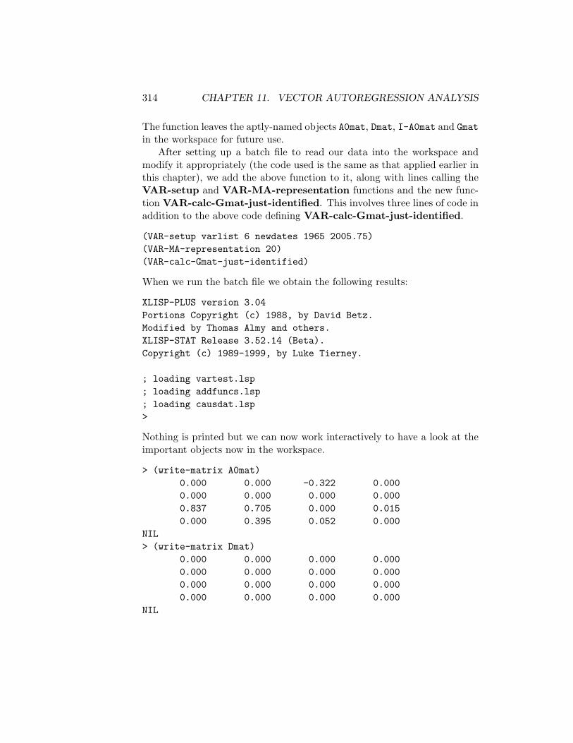
314 CHAPTER 11. VECTOR AUTOREGRESSION ANALYSIS
The function leaves the aptly-named objects A0mat, Dmat, I-A0mat and Gmatin the workspace for future use.
After setting up a batch file to read our data into the workspace andmodify it appropriately (the code used is the same as that applied earlier inthis chapter), we add the above function to it, along with lines calling theVAR-setup and VAR-MA-representation functions and the new func-tion VAR-calc-Gmat-just-identified. This involves three lines of code inaddition to the above code defining VAR-calc-Gmat-just-identified.
(VAR-setup varlist 6 newdates 1965 2005.75)(VAR-MA-representation 20)(VAR-calc-Gmat-just-identified)
When we run the batch file we obtain the following results:
XLISP-PLUS version 3.04Portions Copyright (c) 1988, by David Betz.Modified by Thomas Almy and others.XLISP-STAT Release 3.52.14 (Beta).Copyright (c) 1989-1999, by Luke Tierney.
; loading vartest.lsp; loading addfuncs.lsp; loading causdat.lsp>
Nothing is printed but we can now work interactively to have a look at theimportant objects now in the workspace.
> (write-matrix A0mat)0.000 0.000 -0.322 0.0000.000 0.000 0.000 0.0000.837 0.705 0.000 0.0150.000 0.395 0.052 0.000
NIL> (write-matrix Dmat)
0.000 0.000 0.000 0.0000.000 0.000 0.000 0.0000.000 0.000 0.000 0.0000.000 0.000 0.000 0.000
NIL

11.3. IDENTIFICATION 315
> (print-matrix Dmat)#2a(
( 5.814258E-5 0 0 0 )( 0 6.725789E-6 0 0 )( 0 0 8.132176E-5 0 )( 0 0 0 4.496747E-5)
)NIL> (write-matrix I-A0mat)
1.000 0.000 0.322 0.0000.000 1.000 0.000 0.000
-0.837 -0.705 1.000 -0.0150.000 -0.395 -0.052 1.000
NIL> (write-matrix Gmat)
0.006 -0.001 -0.002 -0.0000.000 0.003 0.000 0.0000.005 0.001 0.007 0.0000.000 0.001 0.000 0.007
NIL> (print-matrix Gmat)#2a(
( 6.005555E-3 -4.680417E-4 -2.289328E-3 -2.629827E-5)( 0.000000 2.593413E-3 0.000000 0.000000 )( 5.028605E-3 1.453221E-3 7.108125E-3 8.165341E-5)( 2.589743E-4 1.099125E-3 3.660700E-4 6.709984E-3)
)NIL
When there are suspiciously located zeros, or very small numbers, in a matrixprinted by the write-matrix function it is best to also print it using theprint-matrix function.
I have written a function called VAR-check-struct-decomp, whichtakes no arguments, to check the calculations above and similar calculationsfor other structural-decompositions. This function uses the Gmat object pro-duced above to recalculate Dmat using the omega object previously in mem-ory and then recalculates a new version of omega. The new and old Dmat andomega objects are printed on the screen—if they are not identical, calcula-tion errors were made in constructing the Var-calc-Gmat-just-identifiedfunction. We can now check our results.
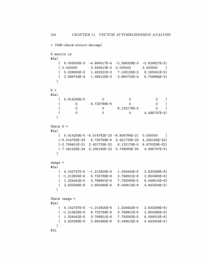
316 CHAPTER 11. VECTOR AUTOREGRESSION ANALYSIS
> (VAR-check-struct-decomp)
G matrix is#2a(
( 6.005555E-3 -4.680417E-4 -2.289328E-3 -2.629827E-5)( 0.000000 2.593413E-3 0.000000 0.000000 )( 5.028605E-3 1.453221E-3 7.108125E-3 8.165341E-5)( 2.589743E-4 1.099125E-3 3.660700E-4 6.709984E-3))
D =#2a(
( 5.814258E-5 0 0 0 )( 0 6.725789E-6 0 0 )( 0 0 8.132176E-5 0 )( 0 0 0 4.496747E-5))
Check D =#2a(
( 5.814258E-5 -5.014782E-23 -6.856784E-21 0.000000 )(-5.014782E-23 6.725789E-6 2.421733E-22 4.235165E-22)(-2.769401E-21 2.421733E-22 8.132176E-5 8.470329E-22)( 7.341228E-24 4.235165E-22 5.738565E-24 4.496747E-5))
omega =#2a(
( 4.152747E-5 -1.213825E-6 1.324442E-5 2.633268E-8)( -1.213825E-6 6.725789E-6 3.768801E-6 2.850485E-6)( 1.324442E-5 3.768801E-6 7.793083E-5 6.049515E-6)( 2.633268E-8 2.850485E-6 6.049515E-6 4.643304E-5))
Check omega =#2a(
( 4.152747E-5 -1.213825E-6 1.324442E-5 2.633268E-8)( -1.213825E-6 6.725789E-6 3.768801E-6 2.850485E-6)( 1.324442E-5 3.768801E-6 7.793083E-5 6.049515E-6)( 2.633268E-8 2.850485E-6 6.049515E-6 4.643304E-5))
NIL
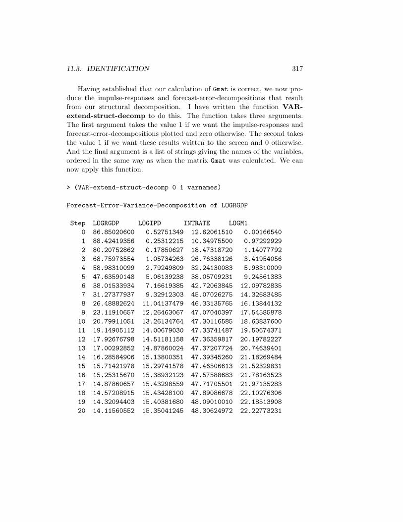
11.3. IDENTIFICATION 317
Having established that our calculation of Gmat is correct, we now pro-duce the impulse-responses and forecast-error-decompositions that resultfrom our structural decomposition. I have written the function VAR-extend-struct-decomp to do this. The function takes three arguments.The first argument takes the value 1 if we want the impulse-responses andforecast-error-decompositions plotted and zero otherwise. The second takesthe value 1 if we want these results written to the screen and 0 otherwise.And the final argument is a list of strings giving the names of the variables,ordered in the same way as when the matrix Gmat was calculated. We cannow apply this function.
> (VAR-extend-struct-decomp 0 1 varnames)
Forecast-Error-Variance-Decomposition of LOGRGDP
Step LOGRGDP LOGIPD INTRATE LOGM10 86.85020600 0.52751349 12.62061510 0.001665401 88.42419356 0.25312215 10.34975500 0.972929292 80.20752862 0.17850627 18.47318720 1.140777923 68.75973554 1.05734263 26.76338126 3.419540564 58.98310099 2.79249809 32.24130083 5.983100095 47.63590148 5.06139238 38.05709231 9.245613836 38.01533934 7.16619385 42.72063845 12.097828357 31.27377937 9.32912303 45.07026275 14.326834858 26.48882624 11.04137479 46.33135765 16.138441329 23.11910657 12.26463067 47.07040397 17.54585878
10 20.79911051 13.26134764 47.30116585 18.6383760011 19.14905112 14.00679030 47.33741487 19.5067437112 17.92676798 14.51181158 47.36359817 20.1978222713 17.00292852 14.87860024 47.37207724 20.7463940114 16.28584906 15.13800351 47.39345260 21.1826948415 15.71421978 15.29741578 47.46506613 21.5232983116 15.25315670 15.38932123 47.57588683 21.7816352317 14.87860657 15.43298559 47.71705501 21.9713528318 14.57208915 15.43428100 47.89086678 22.1027630619 14.32094403 15.40381680 48.09010010 22.1851390820 14.11560552 15.35041245 48.30624972 22.22773231
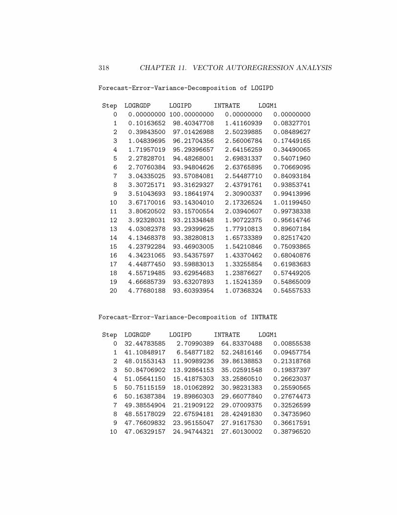
318 CHAPTER 11. VECTOR AUTOREGRESSION ANALYSIS
Forecast-Error-Variance-Decomposition of LOGIPD
Step LOGRGDP LOGIPD INTRATE LOGM10 0.00000000 100.00000000 0.00000000 0.000000001 0.10163652 98.40347708 1.41160939 0.083277012 0.39843500 97.01426988 2.50239885 0.084896273 1.04839695 96.21704356 2.56006784 0.174491654 1.71957019 95.29396657 2.64156259 0.344900655 2.27828701 94.48268001 2.69831337 0.540719606 2.70760384 93.94804626 2.63765895 0.706690957 3.04335025 93.57084081 2.54487710 0.840931848 3.30725171 93.31629327 2.43791761 0.938537419 3.51043693 93.18641974 2.30900337 0.9941399610 3.67170016 93.14304010 2.17326524 1.0119945011 3.80620502 93.15700554 2.03940607 0.9973833812 3.92328031 93.21334848 1.90722375 0.9561474613 4.03082378 93.29399625 1.77910813 0.8960718414 4.13468378 93.38280813 1.65733389 0.8251742015 4.23792284 93.46903005 1.54210846 0.7509386516 4.34231065 93.54357597 1.43370462 0.6804087617 4.44877450 93.59883013 1.33255854 0.6198368318 4.55719485 93.62954683 1.23876627 0.5744920519 4.66685739 93.63207893 1.15241359 0.5486500920 4.77680188 93.60393954 1.07368324 0.54557533
Forecast-Error-Variance-Decomposition of INTRATE
Step LOGRGDP LOGIPD INTRATE LOGM10 32.44783585 2.70990389 64.83370488 0.008555381 41.10848917 6.54877182 52.24816146 0.094577542 48.01553143 11.90989236 39.86138853 0.213187683 50.84706902 13.92864153 35.02591548 0.198373974 51.05641150 15.41875303 33.25860510 0.266230375 50.75115159 18.01062892 30.98231383 0.255905656 50.16387384 19.89860303 29.66077840 0.276744737 49.38554904 21.21909122 29.07009375 0.325265998 48.55178029 22.67594181 28.42491830 0.347359609 47.76609832 23.95155047 27.91617530 0.3661759110 47.06329157 24.94744321 27.60130002 0.38796520
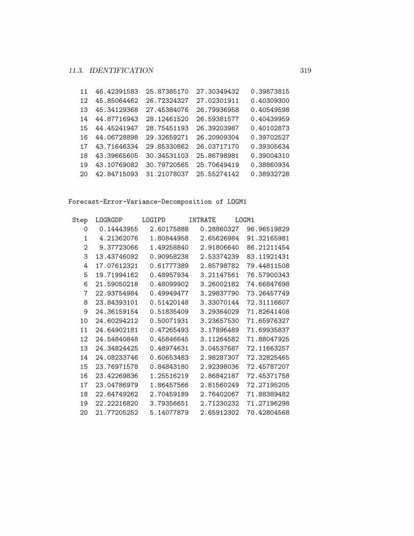
11.3. IDENTIFICATION 319
11 46.42391583 25.87385170 27.30349432 0.3987381512 45.85064462 26.72324327 27.02301911 0.4030930013 45.34129368 27.45384076 26.79936958 0.4054959814 44.87716943 28.12461520 26.59381577 0.4043995915 44.45241947 28.75451193 26.39203987 0.4010287316 44.06728898 29.32659271 26.20909304 0.3970252717 43.71646334 29.85330862 26.03717170 0.3930563418 43.39665605 30.34531103 25.86798981 0.3900431019 43.10769082 30.79720565 25.70649419 0.3886093420 42.84715093 31.21078037 25.55274142 0.38932728
Forecast-Error-Variance-Decomposition of LOGM1
Step LOGRGDP LOGIPD INTRATE LOGM10 0.14443955 2.60175888 0.28860327 96.965198291 4.21362076 1.80844958 2.65626984 91.321659812 9.37723066 1.49258840 2.91806640 86.212114543 13.43746092 0.90958238 2.53374239 83.119214314 17.07612321 0.61777389 2.85798782 79.448115085 19.71994162 0.48957934 3.21147561 76.579003436 21.59050218 0.48099902 3.26002182 74.668476987 22.93754984 0.49949477 3.29837790 73.264577498 23.84393101 0.51420148 3.33070144 72.311166079 24.36159154 0.51835409 3.29364029 71.82641408
10 24.60294212 0.50071931 3.23657530 71.6597632711 24.64902181 0.47265493 3.17896489 71.6993583712 24.54840848 0.45846645 3.11264582 71.8804792513 24.34824425 0.48974631 3.04537687 72.1166325714 24.08233746 0.60653483 2.98287307 72.3282546515 23.76971578 0.84843180 2.92398036 72.4578720716 23.42269836 1.25516219 2.86842187 72.4537175817 23.04786979 1.86457566 2.81560249 72.2719520518 22.64749262 2.70459189 2.76402067 71.8838948219 22.22216820 3.79356651 2.71230232 71.2719629820 21.77205252 5.14077879 2.65912302 70.42804568
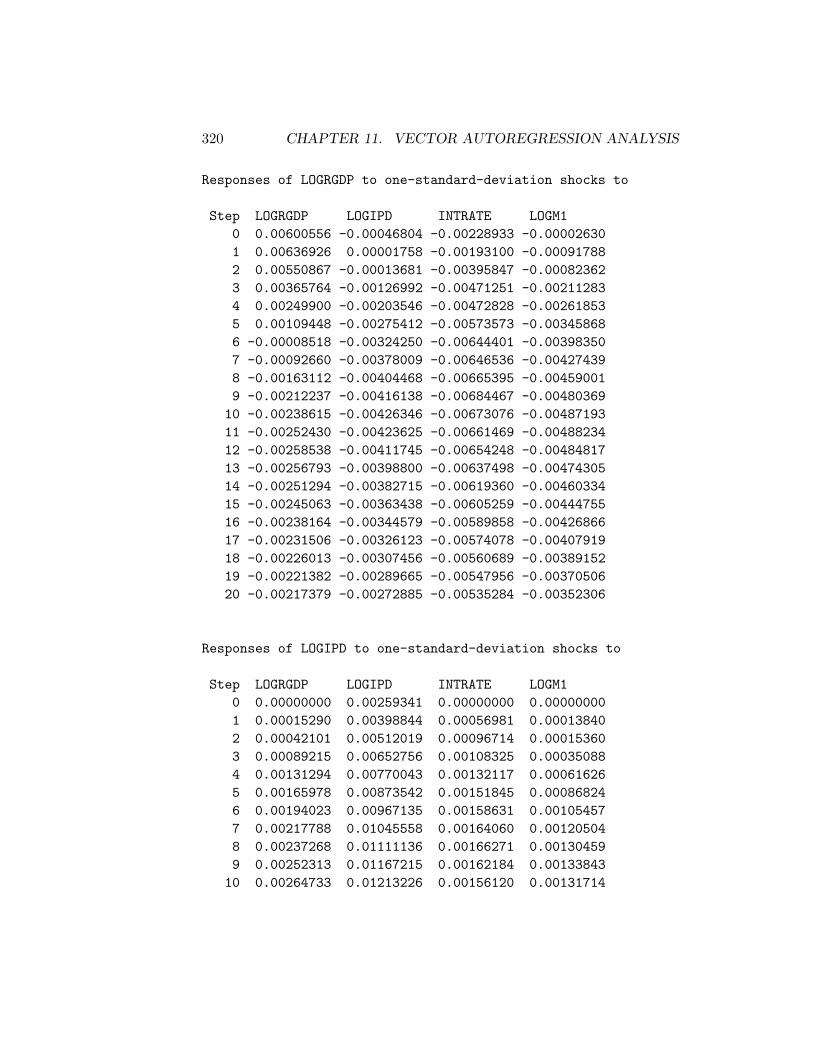
320 CHAPTER 11. VECTOR AUTOREGRESSION ANALYSIS
Responses of LOGRGDP to one-standard-deviation shocks to
Step LOGRGDP LOGIPD INTRATE LOGM10 0.00600556 -0.00046804 -0.00228933 -0.000026301 0.00636926 0.00001758 -0.00193100 -0.000917882 0.00550867 -0.00013681 -0.00395847 -0.000823623 0.00365764 -0.00126992 -0.00471251 -0.002112834 0.00249900 -0.00203546 -0.00472828 -0.002618535 0.00109448 -0.00275412 -0.00573573 -0.003458686 -0.00008518 -0.00324250 -0.00644401 -0.003983507 -0.00092660 -0.00378009 -0.00646536 -0.004274398 -0.00163112 -0.00404468 -0.00665395 -0.004590019 -0.00212237 -0.00416138 -0.00684467 -0.0048036910 -0.00238615 -0.00426346 -0.00673076 -0.0048719311 -0.00252430 -0.00423625 -0.00661469 -0.0048823412 -0.00258538 -0.00411745 -0.00654248 -0.0048481713 -0.00256793 -0.00398800 -0.00637498 -0.0047430514 -0.00251294 -0.00382715 -0.00619360 -0.0046033415 -0.00245063 -0.00363438 -0.00605259 -0.0044475516 -0.00238164 -0.00344579 -0.00589858 -0.0042686617 -0.00231506 -0.00326123 -0.00574078 -0.0040791918 -0.00226013 -0.00307456 -0.00560689 -0.0038915219 -0.00221382 -0.00289665 -0.00547956 -0.0037050620 -0.00217379 -0.00272885 -0.00535284 -0.00352306
Responses of LOGIPD to one-standard-deviation shocks to
Step LOGRGDP LOGIPD INTRATE LOGM10 0.00000000 0.00259341 0.00000000 0.000000001 0.00015290 0.00398844 0.00056981 0.000138402 0.00042101 0.00512019 0.00096714 0.000153603 0.00089215 0.00652756 0.00108325 0.000350884 0.00131294 0.00770043 0.00132117 0.000616265 0.00165978 0.00873542 0.00151845 0.000868246 0.00194023 0.00967135 0.00158631 0.001054577 0.00217788 0.01045558 0.00164060 0.001205048 0.00237268 0.01111136 0.00166271 0.001304599 0.00252313 0.01167215 0.00162184 0.0013384310 0.00264733 0.01213226 0.00156120 0.00131714

11.3. IDENTIFICATION 321
11 0.00275528 0.01250411 0.00148914 0.0012415212 0.00285102 0.01280883 0.00139119 0.0011122713 0.00294149 0.01305218 0.00128028 0.0009385214 0.00303078 0.01324173 0.00116475 0.0007275715 0.00311864 0.01338844 0.00103924 0.0004839416 0.00320522 0.01349755 0.00090594 0.0002146017 0.00329021 0.01357273 0.00076886 -0.0000736818 0.00337161 0.01361889 0.00062626 -0.0003761019 0.00344753 0.01363903 0.00047789 -0.0006878020 0.00351654 0.01363478 0.00032538 -0.00100416
Responses of INTRATE to one-standard-deviation shocks to
Step LOGRGDP LOGIPD INTRATE LOGM10 0.00502860 0.00145322 0.00710813 0.000081651 0.00705365 0.00313728 0.00669702 -0.000407402 0.00704564 0.00435569 0.00285175 -0.000617203 0.00715152 0.00415187 0.00419637 0.000363844 0.00643583 0.00417644 0.00451647 0.000668475 0.00501993 0.00452021 0.00254776 0.000299476 0.00405167 0.00407968 0.00224768 0.000453427 0.00323896 0.00361211 0.00234337 0.000588168 0.00233503 0.00355192 0.00152827 0.000438239 0.00168478 0.00329745 0.00117404 0.00040293
10 0.00128454 0.00297133 0.00123825 0.0004170511 0.00096095 0.00285080 0.00100367 0.0003231912 0.00076285 0.00273549 0.00083031 0.0002486413 0.00069691 0.00258015 0.00087242 0.0002167014 0.00067473 0.00250021 0.00083716 0.0001524715 0.00068364 0.00244576 0.00077066 0.0000843216 0.00072920 0.00236915 0.00078037 0.0000374617 0.00077837 0.00230875 0.00077358 -0.0000148518 0.00081825 0.00225975 0.00073357 -0.0000715419 0.00085430 0.00219772 0.00071138 -0.0001193520 0.00087965 0.00213285 0.00068716 -0.00016556
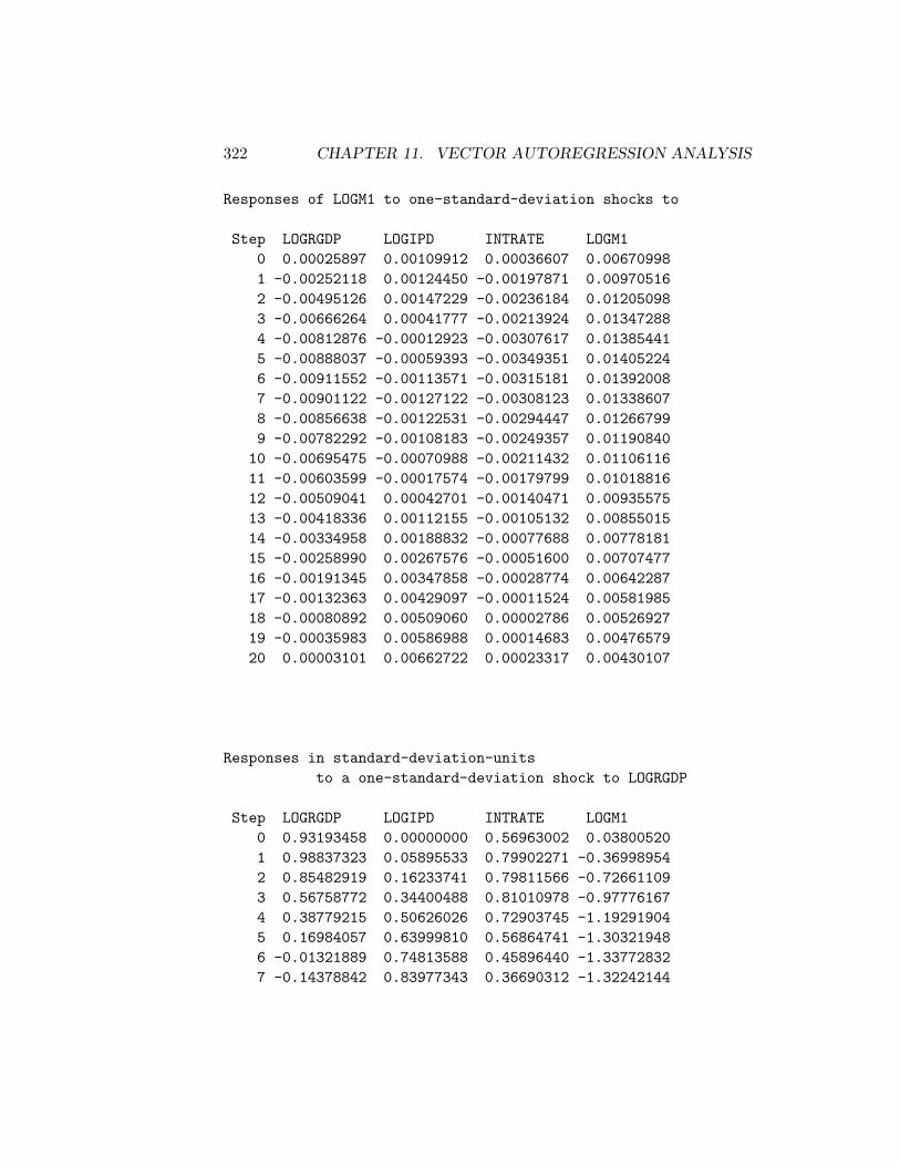
322 CHAPTER 11. VECTOR AUTOREGRESSION ANALYSIS
Responses of LOGM1 to one-standard-deviation shocks to
Step LOGRGDP LOGIPD INTRATE LOGM10 0.00025897 0.00109912 0.00036607 0.006709981 -0.00252118 0.00124450 -0.00197871 0.009705162 -0.00495126 0.00147229 -0.00236184 0.012050983 -0.00666264 0.00041777 -0.00213924 0.013472884 -0.00812876 -0.00012923 -0.00307617 0.013854415 -0.00888037 -0.00059393 -0.00349351 0.014052246 -0.00911552 -0.00113571 -0.00315181 0.013920087 -0.00901122 -0.00127122 -0.00308123 0.013386078 -0.00856638 -0.00122531 -0.00294447 0.012667999 -0.00782292 -0.00108183 -0.00249357 0.0119084010 -0.00695475 -0.00070988 -0.00211432 0.0110611611 -0.00603599 -0.00017574 -0.00179799 0.0101881612 -0.00509041 0.00042701 -0.00140471 0.0093557513 -0.00418336 0.00112155 -0.00105132 0.0085501514 -0.00334958 0.00188832 -0.00077688 0.0077818115 -0.00258990 0.00267576 -0.00051600 0.0070747716 -0.00191345 0.00347858 -0.00028774 0.0064228717 -0.00132363 0.00429097 -0.00011524 0.0058198518 -0.00080892 0.00509060 0.00002786 0.0052692719 -0.00035983 0.00586988 0.00014683 0.0047657920 0.00003101 0.00662722 0.00023317 0.00430107
Responses in standard-deviation-unitsto a one-standard-deviation shock to LOGRGDP
Step LOGRGDP LOGIPD INTRATE LOGM10 0.93193458 0.00000000 0.56963002 0.038005201 0.98837323 0.05895533 0.79902271 -0.369989542 0.85482919 0.16233741 0.79811566 -0.726611093 0.56758772 0.34400488 0.81010978 -0.977761674 0.38779215 0.50626026 0.72903745 -1.192919045 0.16984057 0.63999810 0.56864741 -1.303219486 -0.01321889 0.74813588 0.45896440 -1.337728327 -0.14378842 0.83977343 0.36690312 -1.32242144
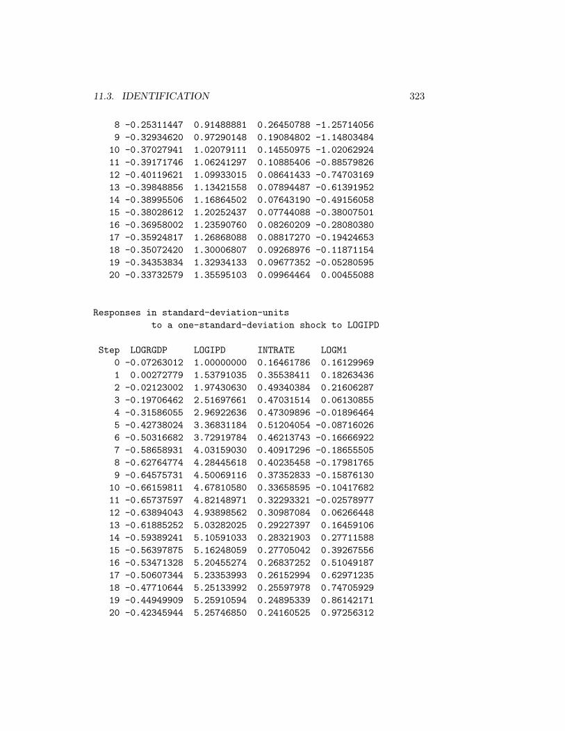
11.3. IDENTIFICATION 323
8 -0.25311447 0.91488881 0.26450788 -1.257140569 -0.32934620 0.97290148 0.19084802 -1.14803484
10 -0.37027941 1.02079111 0.14550975 -1.0206292411 -0.39171746 1.06241297 0.10885406 -0.8857982612 -0.40119621 1.09933015 0.08641433 -0.7470316913 -0.39848856 1.13421558 0.07894487 -0.6139195214 -0.38995506 1.16864502 0.07643190 -0.4915605815 -0.38028612 1.20252437 0.07744088 -0.3800750116 -0.36958002 1.23590760 0.08260209 -0.2808038017 -0.35924817 1.26868088 0.08817270 -0.1942465318 -0.35072420 1.30006807 0.09268976 -0.1187115419 -0.34353834 1.32934133 0.09677352 -0.0528059520 -0.33732579 1.35595103 0.09964464 0.00455088
Responses in standard-deviation-unitsto a one-standard-deviation shock to LOGIPD
Step LOGRGDP LOGIPD INTRATE LOGM10 -0.07263012 1.00000000 0.16461786 0.161299691 0.00272779 1.53791035 0.35538411 0.182634362 -0.02123002 1.97430630 0.49340384 0.216062873 -0.19706462 2.51697661 0.47031514 0.061308554 -0.31586055 2.96922636 0.47309896 -0.018964645 -0.42738024 3.36831184 0.51204054 -0.087160266 -0.50316682 3.72919784 0.46213743 -0.166669227 -0.58658931 4.03159030 0.40917296 -0.186555058 -0.62764774 4.28445618 0.40235458 -0.179817659 -0.64575731 4.50069116 0.37352833 -0.15876130
10 -0.66159811 4.67810580 0.33658595 -0.1041768211 -0.65737597 4.82148971 0.32293321 -0.0257897712 -0.63894043 4.93898562 0.30987084 0.0626644813 -0.61885252 5.03282025 0.29227397 0.1645910614 -0.59389241 5.10591033 0.28321903 0.2771158815 -0.56397875 5.16248059 0.27705042 0.3926755616 -0.53471328 5.20455274 0.26837252 0.5104918717 -0.50607344 5.23353993 0.26152994 0.6297123518 -0.47710644 5.25133992 0.25597978 0.7470592919 -0.44949909 5.25910594 0.24895339 0.8614217120 -0.42345944 5.25746850 0.24160525 0.97256312

324 CHAPTER 11. VECTOR AUTOREGRESSION ANALYSIS
Responses in standard-deviation-unitsto a one-standard-deviation shock to INTRATE
Step LOGRGDP LOGIPD INTRATE LOGM10 -0.35525505 0.00000000 0.80519380 0.053721811 -0.29964949 0.21971284 0.75862487 -0.290381652 -0.61427066 0.37292148 0.32304014 -0.346606473 -0.73128067 0.41769220 0.47535616 -0.313939004 -0.73372878 0.50943409 0.51161623 -0.451436955 -0.89006270 0.58550246 0.28860466 -0.512683056 -0.99997286 0.61166767 0.25461294 -0.462536497 -1.00328600 0.63260390 0.26545219 -0.452179348 -1.03255095 0.64112955 0.17311959 -0.432109359 -1.06214703 0.62537070 0.13299300 -0.3659386710 -1.04447081 0.60198483 0.14026669 -0.3102826611 -1.02645890 0.57420138 0.11369417 -0.2638607612 -1.01525429 0.53643376 0.09405569 -0.2061457113 -0.98926070 0.49366505 0.09882651 -0.1542844714 -0.96111524 0.44912054 0.09483130 -0.1140096315 -0.93923270 0.40072158 0.08729873 -0.0757237916 -0.91533446 0.34932403 0.08839882 -0.0422269917 -0.89084653 0.29646598 0.08762921 -0.0169119718 -0.87006963 0.24148170 0.08309707 0.0040892219 -0.85031138 0.18427148 0.08058336 0.0215475020 -0.83064718 0.12546274 0.07784053 0.03421884
Responses in standard-deviation-unitsto a one-standard-deviation shock to LOGM1
Step LOGRGDP LOGIPD INTRATE LOGM10 -0.00408093 0.00000000 0.00924953 0.984709091 -0.14243616 0.05336552 -0.04614985 1.424259002 -0.12780826 0.05922796 -0.06991545 1.768515533 -0.32786649 0.13529538 0.04121531 1.977183294 -0.40633970 0.23762363 0.07572273 2.033173645 -0.53671375 0.33478564 0.03392359 2.062206496 -0.61815517 0.40663355 0.05136288 2.04281079

11.3. IDENTIFICATION 325
7 -0.66329510 0.46465539 0.06662574 1.964443418 -0.71227239 0.50303946 0.04964149 1.859063429 -0.74543066 0.51608705 0.04564293 1.74759079
10 -0.75602008 0.50787787 0.04724236 1.6232558011 -0.75763483 0.47872126 0.03661039 1.4951418512 -0.75233294 0.42888253 0.02816572 1.3729832813 -0.73602073 0.36188714 0.02454686 1.2547584114 -0.71434040 0.28054716 0.01727140 1.1420029415 -0.69016595 0.18660238 0.00955213 1.0382423716 -0.66240478 0.08274759 0.00424286 0.9425741117 -0.63300404 -0.02841092 -0.00168238 0.8540791018 -0.60388051 -0.14502170 -0.00810370 0.7732806419 -0.57494615 -0.26521049 -0.01351975 0.6993936720 -0.54670350 -0.38719642 -0.01875449 0.63119354
NIL
The responses of all the variables, in own standard-deviation units, toshocks to each variable in turn are plotted in Figure 19. A careful comparisonof that figure with Figure 17 reveals that the two decompositions result inmuch the same pattern of impulse responses, the important exception beingthat in the initial period real GDP falls in response to an interest rate shockin Figure 19, whereas it is unaffected in the current period in Figure 17.
An alternative way of doing structural-decompositions that can producea satisfactory result even when the system is over-determined—implying, inour example above, more than 10 zero entries and less than six parameterentries in the A0 matrix—is to maximize the log likelihood function
log|I− A0|2 −m∑
i=1
log [(I− A0)M(I− A0)′]ii
where M is the matrix omega left in the workspace by the VAR-MA-representation function and A0 is the measure of A0 to be achieved bythe maximisation process.
To perform this estimation we need to write another function, which willagain be specific to the maximisation problem at hand, that can be usedwith either the newtonmax function or the nelmeadmax function provided inXLispStat. This function, which we will call varstd, is also saved as a tem-plate in the file strucdec.lsp from where it can be modified appropriatelyand used again in other situations.
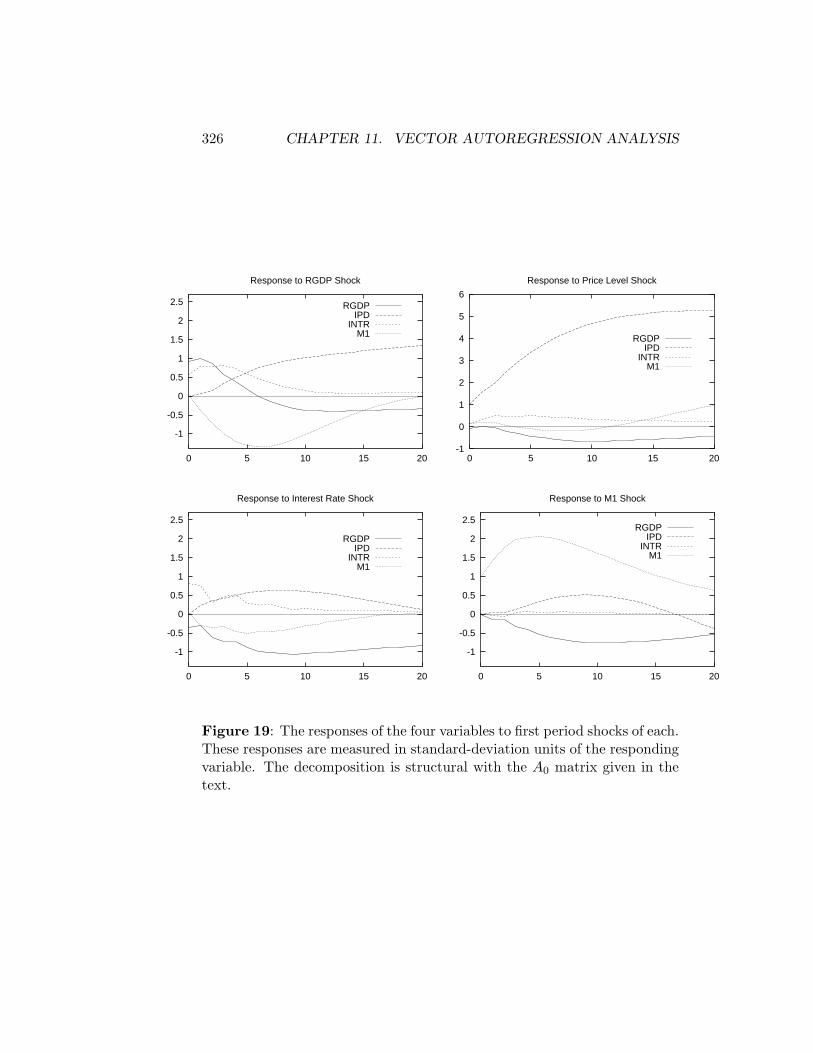
326 CHAPTER 11. VECTOR AUTOREGRESSION ANALYSIS
-1
-0.5
0
0.5
1
1.5
2
2.5
0 5 10 15 20
Response to RGDP Shock
RGDPIPD
INTRM1
-1
0
1
2
3
4
5
6
0 5 10 15 20
Response to Price Level Shock
RGDPIPD
INTRM1
-1
-0.5
0
0.5
1
1.5
2
2.5
0 5 10 15 20
Response to Interest Rate Shock
RGDPIPD
INTRM1
-1
-0.5
0
0.5
1
1.5
2
2.5
0 5 10 15 20
Response to M1 Shock
RGDPIPD
INTRM1
Figure 19: The responses of the four variables to first period shocks of each.These responses are measured in standard-deviation units of the respondingvariable. The decomposition is structural with the A0 matrix given in thetext.

11.3. IDENTIFICATION 327
(defun varstd (theta)(let* ((alf02 (select theta 0))
(alf20 (select theta 1))(alf21 (select theta 2))(alf23 (select theta 3))(alf31 (select theta 4))(alf32 (select theta 5))) ; first end of let*(def alfmat (make-array ’(4 4) :initial-element 0))(def idmat (identity-matrix numvars))(setf (aref alfmat 0 2) alf02)(setf (aref alfmat 2 0) alf20)(setf (aref alfmat 2 1) alf21)(setf (aref alfmat 2 3) alf23)(setf (aref alfmat 3 1) alf31)(setf (aref alfmat 3 2) alf32)(def thetmat (- idmat alfmat))
(- (log (^ (determinant thetmat) 2))(sum (log (diagonal (matmult thetmat omega (transpose thetmat))))))) ; second end of let*
) ; end of function varstd
We then call a function I wrote, called VAR-maxlike-calc-Gmat, whichcalls the above varstd function and requires in the workspace a list calledthetlist giving initial values of the A0 elements to be determined, orderedleft-to-right, row-by-row, top-to-bottom. To obtain this list from the objectA0mat left in the workspace by the just-identified structural-decompositionabove we call another function I wrote, VAR-calc-thetlist, which takesno arguments. The function VAR-maxlike-calc-Gmat takes a single ar-gument, zero if the newtonmax function is to be applied or unity if thenelmeadmax function is to be applied instead. The best procedure is to tryto find optimum first using the newtonmax function and resort to the otherfunction if these initial efforts fail.
> (VAR-calc-thetlist 0)THETLIST> THETLIST(-0.3220719938737918 0.8366593493548039 0.704798332039390.015448039667841666 0.3949559732790447 0.05150022412303335)
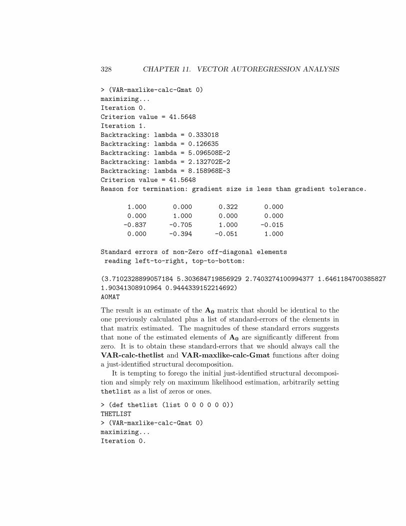
328 CHAPTER 11. VECTOR AUTOREGRESSION ANALYSIS
> (VAR-maxlike-calc-Gmat 0)maximizing...Iteration 0.Criterion value = 41.5648Iteration 1.Backtracking: lambda = 0.333018Backtracking: lambda = 0.126635Backtracking: lambda = 5.096508E-2Backtracking: lambda = 2.132702E-2Backtracking: lambda = 8.158968E-3Criterion value = 41.5648Reason for termination: gradient size is less than gradient tolerance.
1.000 0.000 0.322 0.0000.000 1.000 0.000 0.000
-0.837 -0.705 1.000 -0.0150.000 -0.394 -0.051 1.000
Standard errors of non-Zero off-diagonal elementsreading left-to-right, top-to-bottom:
(3.7102328899057184 5.303684719856929 2.7403274100994377 1.64611847003858271.90341308910964 0.9444339152214692)A0MAT
The result is an estimate of the A0 matrix that should be identical to theone previously calculated plus a list of standard-errors of the elements inthat matrix estimated. The magnitudes of these standard errors suggeststhat none of the estimated elements of A0 are significantly different fromzero. It is to obtain these standard-errors that we should always call theVAR-calc-thetlist and VAR-maxlike-calc-Gmat functions after doinga just-identified structural decomposition.
It is tempting to forego the initial just-identified structural decomposi-tion and simply rely on maximum likelihood estimation, arbitrarily settingthetlist as a list of zeros or ones.
> (def thetlist (list 0 0 0 0 0 0))THETLIST> (VAR-maxlike-calc-Gmat 0)maximizing...Iteration 0.

11.3. IDENTIFICATION 329
Criterion value = 41.4359Iteration 1.Criterion value = 41.5558Iteration 2.Backtracking: lambda = 0.259378Criterion value = 41.5620Iteration 3.Criterion value = 41.5642Iteration 4.Criterion value = 41.5648Iteration 5.Criterion value = 41.5648Iteration 6.Criterion value = 41.5648Reason for termination: gradient size is less than gradient tolerance.
1.000 0.000 0.322 0.0000.000 1.000 0.000 0.000-0.837 -0.705 1.000 -0.0150.000 -0.394 -0.051 1.000
Standard errors of non-Zero off-diagonal elementsreading left-to-right, top-to-bottom:
(#C(0.0 1.0343693636602518) #C(0.0 1.9575078619747457) 1.9446540242557864#C(0.0 3.3416950133122287) 1.6567713599448393 #C(0.0 1.9949100906025918))A0MAT
We get the correct values for the matrix elements, yet all but one of the stan-dard errors are imaginary numbers. Application of the nelmeadmax functionby using 1 instead of 0 as the argument in VAR-maxlike-calc-Gmat yieldsan identical result. Alternatively, if we initialise all the elements of thetlistat unity we get garbage with the newtonmax application, the iteration limithaving been exceeded.
> (def thetlist (list 1 1 1 1 1 1))THETLIST(VAR-maxlike-calc-Gmat 0)maximizing...Iteration 0.Criterion value = 39.1633

330 CHAPTER 11. VECTOR AUTOREGRESSION ANALYSIS
Iteration 1.Criterion value = 39.7078Iteration 2.Criterion value = 40.0347Iteration 3.Criterion value = 40.2609Iteration 4.Criterion value = 40.5031Iteration 5.Criterion value = 40.9342Iteration 6.Backtracking: lambda = 0.492226Criterion value = 41.1692Iteration 7.Criterion value = 41.3788Iteration 8.Criterion value = 41.4693..........Iteration 97.Criterion value = 41.5373Iteration 98.Criterion value = 41.5373Iteration 99.Criterion value = 41.5373Iteration 100.Criterion value = 41.5373Reason for termination: iteration limit exceeded.
1.000 0.000 -1377.261 0.0000.000 1.000 0.000 0.000
-5.445 -1.529 1.000 -0.0340.000 -0.389 -0.058 1.000
Standard errors of non-Zero off-diagonal elementsreading left-to-right, top-to-bottom:
(0.3249537545448562 0.4451422015073173 3.19260682787145540.46089240276344035 3.256804838519031 0.3375676002252116)NIL
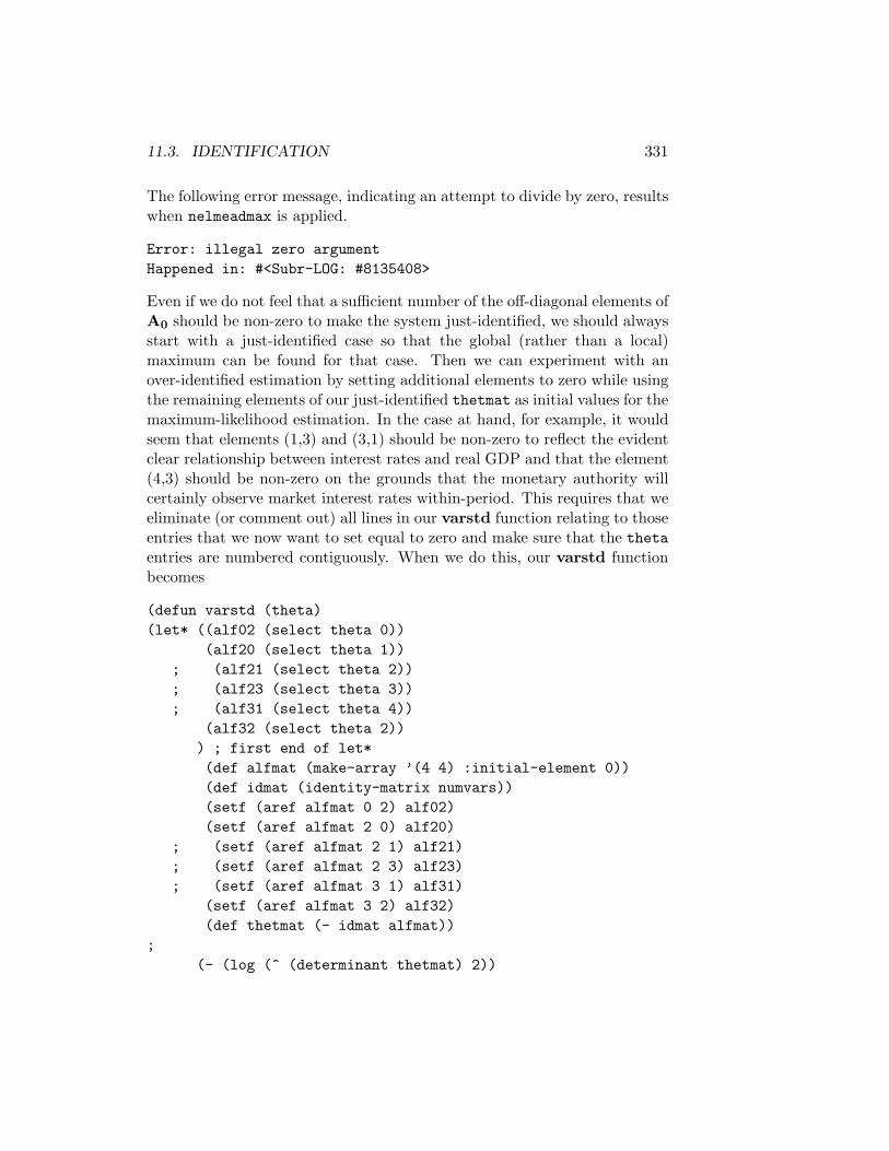
11.3. IDENTIFICATION 331
The following error message, indicating an attempt to divide by zero, resultswhen nelmeadmax is applied.
Error: illegal zero argumentHappened in: #<Subr-LOG: #8135408>
Even if we do not feel that a sufficient number of the off-diagonal elements ofA0 should be non-zero to make the system just-identified, we should alwaysstart with a just-identified case so that the global (rather than a local)maximum can be found for that case. Then we can experiment with anover-identified estimation by setting additional elements to zero while usingthe remaining elements of our just-identified thetmat as initial values for themaximum-likelihood estimation. In the case at hand, for example, it wouldseem that elements (1,3) and (3,1) should be non-zero to reflect the evidentclear relationship between interest rates and real GDP and that the element(4,3) should be non-zero on the grounds that the monetary authority willcertainly observe market interest rates within-period. This requires that weeliminate (or comment out) all lines in our varstd function relating to thoseentries that we now want to set equal to zero and make sure that the thetaentries are numbered contiguously. When we do this, our varstd functionbecomes
(defun varstd (theta)(let* ((alf02 (select theta 0))
(alf20 (select theta 1)); (alf21 (select theta 2)); (alf23 (select theta 3)); (alf31 (select theta 4))
(alf32 (select theta 2))) ; first end of let*(def alfmat (make-array ’(4 4) :initial-element 0))(def idmat (identity-matrix numvars))(setf (aref alfmat 0 2) alf02)(setf (aref alfmat 2 0) alf20)
; (setf (aref alfmat 2 1) alf21); (setf (aref alfmat 2 3) alf23); (setf (aref alfmat 3 1) alf31)
(setf (aref alfmat 3 2) alf32)(def thetmat (- idmat alfmat))
;(- (log (^ (determinant thetmat) 2))
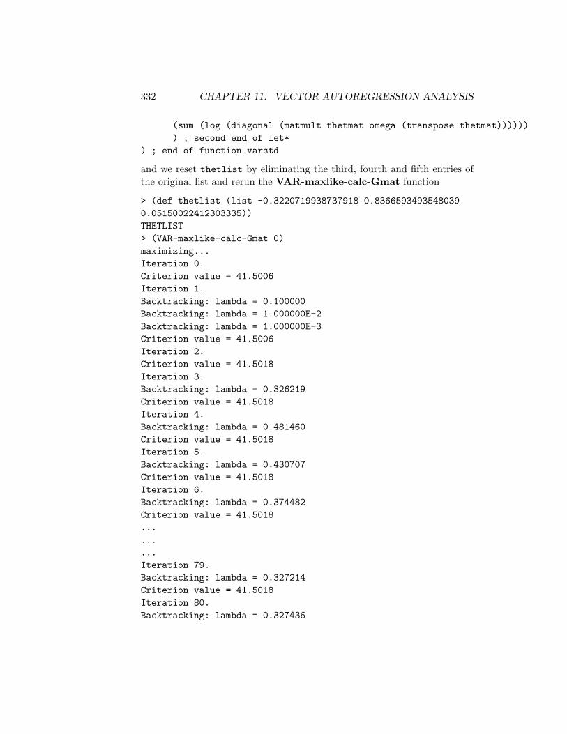
332 CHAPTER 11. VECTOR AUTOREGRESSION ANALYSIS
(sum (log (diagonal (matmult thetmat omega (transpose thetmat))))))) ; second end of let*
) ; end of function varstd
and we reset thetlist by eliminating the third, fourth and fifth entries ofthe original list and rerun the VAR-maxlike-calc-Gmat function
> (def thetlist (list -0.3220719938737918 0.83665934935480390.05150022412303335))THETLIST> (VAR-maxlike-calc-Gmat 0)maximizing...Iteration 0.Criterion value = 41.5006Iteration 1.Backtracking: lambda = 0.100000Backtracking: lambda = 1.000000E-2Backtracking: lambda = 1.000000E-3Criterion value = 41.5006Iteration 2.Criterion value = 41.5018Iteration 3.Backtracking: lambda = 0.326219Criterion value = 41.5018Iteration 4.Backtracking: lambda = 0.481460Criterion value = 41.5018Iteration 5.Backtracking: lambda = 0.430707Criterion value = 41.5018Iteration 6.Backtracking: lambda = 0.374482Criterion value = 41.5018.........Iteration 79.Backtracking: lambda = 0.327214Criterion value = 41.5018Iteration 80.Backtracking: lambda = 0.327436

11.3. IDENTIFICATION 333
Criterion value = 41.5018Iteration 81.Backtracking: lambda = 0.323776Criterion value = 41.5018Reason for termination: gradient size is less than gradient tolerance.
1.000 0.000 0.867 0.0000.000 1.000 0.000 0.000-1.523 0.000 1.000 0.0000.000 0.000 -0.077 1.000
Standard errors of non-Zero off-diagonal elementsreading left-to-right, top-to-bottom:
(#C(0.0 45.668017134873985) #C(0.0 66.60451111932105) 0.5439894547366717)
Two of the three standard errors are imaginary numbers! Using the nelmead-max function gives the same result.
If we impose zero restrictions on all coefficients except that giving theeffect of the interest rate on real GDP we get a maximum, again with a highstandard-error. The batch code is
(defun varstd (theta)(let* ((alf02 (select theta 0))
) ; first end of let*(def alfmat (make-array ’(4 4) :initial-element 0))(def idmat (identity-matrix numvars))(setf (aref alfmat 0 2) alf02)(def thetmat (- idmat alfmat))(- (log (^ (determinant thetmat) 2))(sum (log (diagonal (matmult thetmat omega(transpose thetmat))))))) ; second end of let*
) ; end of function varstd(def thetlist (list -0.3220719938737918))(VAR-maxlike-calc-Gmat 0)
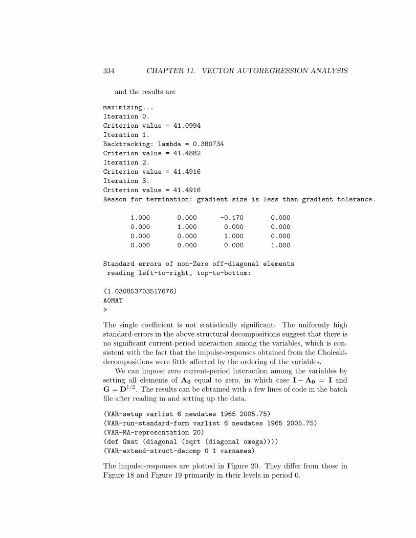
334 CHAPTER 11. VECTOR AUTOREGRESSION ANALYSIS
and the results are
maximizing...Iteration 0.Criterion value = 41.0994Iteration 1.Backtracking: lambda = 0.380734Criterion value = 41.4882Iteration 2.Criterion value = 41.4916Iteration 3.Criterion value = 41.4916Reason for termination: gradient size is less than gradient tolerance.
1.000 0.000 -0.170 0.0000.000 1.000 0.000 0.0000.000 0.000 1.000 0.0000.000 0.000 0.000 1.000
Standard errors of non-Zero off-diagonal elementsreading left-to-right, top-to-bottom:
(1.030853703517676)A0MAT>
The single coefficient is not statistically significant. The uniformly highstandard-errors in the above structural decompositions suggest that there isno significant current-period interaction among the variables, which is con-sistent with the fact that the impulse-responses obtained from the Choleski-decompositions were little affected by the ordering of the variables.
We can impose zero current-period interaction among the variables bysetting all elements of A0 equal to zero, in which case I−A0 = I andG = D1/2. The results can be obtained with a few lines of code in the batchfile after reading in and setting up the data.
(VAR-setup varlist 6 newdates 1965 2005.75)(VAR-run-standard-form varlist 6 newdates 1965 2005.75)(VAR-MA-representation 20)(def Gmat (diagonal (sqrt (diagonal omega))))(VAR-extend-struct-decomp 0 1 varnames)
The impulse-responses are plotted in Figure 20. They differ from those inFigure 18 and Figure 19 primarily in their levels in period 0.

11.3. IDENTIFICATION 335
-1
-0.5
0
0.5
1
1.5
2
2.5
0 5 10 15 20
Response to RGDP Shock
RGDPIPD
INTRM1
-1
0
1
2
3
4
5
6
0 5 10 15 20
Response to Price Level Shock
RGDPIPD
INTRM1
-1
-0.5
0
0.5
1
1.5
2
2.5
0 5 10 15 20
Response to Interest Rate Shock
RGDPIPD
INTRM1
-1
-0.5
0
0.5
1
1.5
2
2.5
0 5 10 15 20
Response to M1 Shock
RGDPIPD
INTRM1
Figure 20: The responses of the four variables to first period shocks ofeach. These responses are measured in standard-deviation units of the re-sponding variable. The decomposition is structural with all current-periodinteractions of the variables set equal to zero.

336 CHAPTER 11. VECTOR AUTOREGRESSION ANALYSIS
11.3.3 Blanchard-Quah Decompositions
For certain types of problems it is useful to decompose Ω by a method de-veloped by Blanchard and Quah.7 Their method assumes a two variableVAR with two equations and two types of shock, real and nominal, thatare statistically independent of each other and affect both equations. Herewe take the two variables to be the real and nominal exchange rates. ABlanchard-Quah decomposition identifies the real and nominal shocks un-der the assumption that one type of shock, in our case the nominal shock,has a temporary but no permanent effect on the level of one of the variables,in our case the real exchange rate, and a permanent effect on the level ofthe other variable, the nominal exchange rate. The other type of shock,a real shock, has permanent effects on the levels of both variables. Nei-ther the real nor the nominal shocks have permanent long-run effects on thefirst differences of either of the variables. Decomposition is accomplishedby imposing one restriction on the two-variable VAR—the restriction, inour case, that nominal shocks can have no permanent effects on the levelof the real exchange rate. In using the Blanchard-Quah method, our inter-est is directed more toward decomposition of the standard-form errors intoorthogonal structural errors than to obtaining the elements of the matrixA0.
We are still interested in the matrix G which will reduce the moving av-erage representation (11.16) to (11.17) and in particular enable us to obtainthe orthogonal errors
et−j = G−1ut−j .
Now, however, the identifying restriction is that the sum of the upper leftcorner elements of the (now 2 × 2) matrices Z0 = C0G, Z1 = C1G, Z2 =C2G, · · · · · · , Zn = CnG, be equal to zero. This assumes that the realexchange rate equation is the first equation and that the nominal shock isthe first shock. Had we wanted to assume that the nominal shock is thesecond shock the identifying restriction would have been that the sum ofthe upper right corner elements of the above matrices is zero. There is norequirement that the nominal shock be identified with the nominal exchangerate variable. The statistical results will be the same whether the nominalshock is the first or the second shock.
The sum of the matrices C0, C1, C2, · · · · · · , etc. can be obtainedby calculating the sum of the corresponding elements in equation (11.15)
7Olivier Jean Blanchard and Danny Quah, “The Dynamic Effects of Aggregate Demandand Supply Disturbances,” American Economic Review, 79, September 1989, 655–73.

11.3. IDENTIFICATION 337
using the relationship
S = Imp + B + B 2 + B 3 + B 4 + · · · · · · · · · · · ·= (Imp − B)−1. (11.57)
and stripping off the upper-left 2 × 2 matrix of elements from S using the(now 2×2p) matrix J used to obtain equation (11.11) from equation (11.17).We thus obtain
S = JSJ ′. (11.58)
The Blanchard-Quah condition is that the upper left element of the 2 × 2matrix SG (which is the sum of the upper-left elements of the Cj matricesafter each has been post-multiplied by G) be zero.
In addition, the G matrix must have the property GG′ = Ω. A Choleskidecomposition of Ω produces a matrix with this property, as does the trans-formation of (I−A)−1 by (11.51) we made in the structural VAR calcula-tions. It turns out that any orthogonal transformation of a matrix obtainedfrom a Choleski decomposition will also possess this property. The pro-cedure here is therefore to make a Choleski decomposition of Ω to obtainsome matrix E which we can then transform using some orthogonal matrixP to impose upon it the Blanchard-Quah condition and thereby obtain thedesired matrix G. The two requirements are that
GG′ = EP(EP)′
= EPP′E′
= EE′ = Ω (11.59)
since orthogonality of P implies PP′ = I, and that the upper left cornerelement of the (2× 2) matrix
SG = SEP = SEP = HP (11.60)
equal zero, where H = SE. Expanding the latter condition we have8
h11p11 + h12p21 = 0. (11.61)
8Were we to designate the second shock as the nominal shock, this condition wouldbecome
h11p21 + h12p22 = 0.

338 CHAPTER 11. VECTOR AUTOREGRESSION ANALYSIS
From the fact that PP′ = I we obtain[
p 211 + p 2
12 p11p21 + p12p22
p21p11 + p22p12 p 221 + p 2
22
]=
[1 00 1
]
which yields the three conditions
p 211 + p 2
12 = 1 (11.62)p11p21 = − p12p22 (11.63)
p 221 + p 2
22 = 1 (11.64)
Given the values of S and E and H, calculated from the data, the fourequations (11.61) through (11.64) solve for the four elements of P. Thelatter matrix can then be multiplied by E to obtain G. Using this matrix,the impulse-response functions can be calculated from (11.17).9
These calculations are illustrated using monthly data on the Canada/U.S.real and nominal exchange rates. The real exchange rate and ratio of Cana-dian to U.S. price levels data are contained in the file causdat.lsp. Fromthese, an appropriate nominal exchange rate series can can be obtained and,after putting all three series on a base of 1990 = 100, the logarithms of thetwo exchange rate series can be taken.
(def causnex (/ causrex causnpr))(def causrex (base causrex datesmo 1990.0 12))(def causnex (base causnex datesmo 1990.0 12))(def nex (log causnex))(def rex (log causrex))
9In calculating the elements of the matrix P it is useful to rearrange (11.61) to obtain
p11 = −h12
h11p21 = w p21
and then square both sides of this equation and substitute the resulting expression for p211
into the square of equation (11.63). From there it can be shown that
p12 = p21 =
√1
1 + w2,
which will be positive regardless of the sign of w. Multiplication of p21 by w then yieldsp11. Using these results along with (11.63), it can then be shown that
p22 = −p11.
11.3. IDENTIFICATION 339
Then we extract from these series-lists, using our set-time-series function,the portions that we will need later.
(def actser1 (set-time-series rex datesmo 1962.0 2005.9166 0))(def actser2 (set-time-series nex datesmo 1962.0 2005.9166 0))(def nprser (set-time-series causnpr datesmo 1974.0 2005.9166 0))
Next, we take the first differences of the series and adjust the datelist ac-cordingly.10
(def difdates (remove-first 1 datesmo))(def drex (difference rex))(def dnex (difference nex))(def dnpr (difference (log nprser)))
After constructing appropriate lists of variables and of their names, we at-tack the problem of determining the appropriate lag length using our VAR-lag-length function. Based on the resulting printout (not shown) we choosea lag-length of 18 months—the longest lag length supported by our tests ofthe first-differences and levels of the two series. The appropriate code is
(def varlstdca (list drex dnex))(def varnamesd (list "drex" "dnex"))(VAR-lag-length varlstdca varnamesd 24 difdates 1972.0 2005.9166)(def varlstlca (list rex nex))(def varnamesl (list "rex" "nex"))(VAR-lag-length varlstlca varnamesl 24 difdates 1972.0 2005.9166)
Before calling our VAR functions we need to put in the workspace some liststhat they will require.
(def varlist (list drex dnex))(def filelist (list "rexch" "nexch"))(def lablist (list "real exch rate" "nom exch rate"))(def shocklist (list "mon shk" "real shk"))(def histlabs (list "real exch rate -- money (pts) and real shocks""nom exch rate -- money (pts) and real shocks"))
Apart from varlist, which is a list of the lists of the two variables that willbe in our VAR, the above lists represent various labels that will be needed.
10The decision to use logarithms as well as first differences (which should always beused) follows from the work of Enders—see page 338 of the book previously cited.
340 CHAPTER 11. VECTOR AUTOREGRESSION ANALYSIS
The first list is a list of the file names, while the other three are labelsgiving appropriate names of the variables and shocks that will be usefullater on. The list filelist will not be used until we do bootstrappingto obtain confidence intervals. After running the batch file that we are, ineffect, constructing here it should be apparent why particular forms of labelswere chosen, although many possible alternative expressions could have beenused.
We can now run the VAR, starting as usual with the VAR-setupand VAR-MA-representation functions and adopting 20 steps for theimpulse-responses and forecast-error-variance decompositions. Next we callthe function I wrote to perform a Blanchard-Quah decomposition. Thisfunction VAR-BlanQuah-decomp, which takes no arguments, follows theanalytical framework presented above. It uses the variance-covariance ma-trix omega left in memory by the previous VAR functions as well as a matrixlitS which the previous functions will also have created. The first of the twoshocks is designated as the nominal shock. Three lists with the same namesas the corresponding lists produced by Choleski and structural decomposi-tions, rofmats, rtomats and fevmats, containing four matrices each, arealso left in the workspace. The same functions used to print out and plotour earlier VARs can also be used here.
(VAR-setup varlist 18 difdates 1974.0 2005.9166)(VAR-MA-representation 20)(VAR-BlanQuah-decomp)(VAR-print-forecast-error-variance-decompositions lablist)(VAR-print-impulse-responses lablist)(VAR-plot-impulse-responses-of lablist)(VAR-plot-impulse-responses-to lablist)
The printing and plotting functions draw on the matrices rofmats, rtomatsand fevmats, already in the workspace and take as their single argument thelist of labels lablist that we have already read into the workspace. Whenthese functions are used to print and plot results obtained by a Blanchard-Quah decomposition, they require a list of strings called shocklist thatgives the names of the shocks—this list was also previously read into theworkspace.
In addition to the impulse-responses and forecast-error-variance decom-positions, historical decompositions of the actual movements of the two vari-ables over the time-period being studied into portions caused by the separateshocks is also of interest in Blanchard-Quah VARs. I have written two func-tions, VAR-blanquah-history and bq-exch-rate-history to calculate,
11.3. IDENTIFICATION 341
print and plot the resulting time-series. The first of these functions takestwo arguments—the first is set at 1 or zero according to whether or not thehistorical decompositions are to be plotted on the screen, and the second isthe number of bootstrap runs if subsequent bootstrapping to obtain confi-dence intervals is to be undertaken. If bootstrapping is to take place and thenumber of bootstrap runs is therefore greater than zero, the historical de-compositions are automatically plotted. This function must always be calledprior to bootstrapping, before the initial Gmat matrix is overwritten. It pro-duces a list of historical decompositions of the variables called histlists,ordered by variable and for each variable by shock, first nominal and thenreal, giving the cumulative percentage variation of the variable around zeroresulting from the respective shocks. These are always written to the filebqhist.mat, which will be overwritten each time the function is called. Italso leaves in the workspace a number of objects that will be used by thesecond function bq-exch-rate-history, if it is called.
This second function, which is specific to Blanchard-Quah decomposi-tions involving real and nominal exchange rates of the sort we are doinghere, modifies the results of the previous function appropriately to incor-porate trends in the historical decompositions. All the trend in the realexchange rate is applied to the real shock and none of it to the correspond-ing monetary shock. In the case of the nominal exchange rate the differencebetween trends in the actual nominal and real exchange rates is assigned tothe monetary shock and the remaining movements of the nominal exchangerate are assigned to the real shock. All series are converted from the log-arithms back to their original scale and their average values are set equalto 100. If the function’s single argument is set equal to unity, they plottedon the screen. These series are always written to the file bqhist.mat, over-writing the file of the same name created by the function VAR-blanquah-history. This data file can be read by Gnuplot. The variables this filecontains are left in the workspace as the lists actrex, actnex (the actualseries), rexmonshk, rexrealshk, nexmonshk, nexrealshk and nprser. Thelast of these series, which is the domestic/foreign price-level ratio, is notused by either of the above functions, but must be present in the workspacebefore the functions are called—the bq-exch-rate-history function merelytakes it from the workspace and incorporates it in the output file. We cancall either the first or both of these functions in our batch file any time afterthe VAR-BlanQuah-decomp function but before any bootstrapping.
(VAR-blanquah-history 1 0)(bq-exch-rate-history 1)
The historical decompositions of the Canada/U.S. real exchange rates areshown in Figure 21.

342 CHAPTER 11. VECTOR AUTOREGRESSION ANALYSIS
70
80
90
100
110
120
130
140
150
1975 1980 1985 1990 1995 2000 2005
1974-2005 = 100
HISTORICAL DECOMPOSITION: REAL EXCHANGE RATE
Actual LevelDue to Money Shocks
Due to Real Shocks
70
80
90
100
110
120
130
140
150
1975 1980 1985 1990 1995 2000
1974-2005 = 100
HISTORICAL DECOMPOSITION: NOMINAL EXCHANGE RATE
Actual LevelDue to Money Shocks
Due to Real Shocks
Figure 21: Blanchard-Quah-VAR historical decompositions of Canada’sreal and nominal exchange rates with respect to the U.S. dollar into themovements attributable to real and money shocks.

11.4. BOOTSTRAPPING CONFIDENCE INTERVALS 343
11.4 Bootstrapping Confidence Intervals
Finally, we turn to the problem of calculating confidence intervals for ourimpulse-responses and forecast-error-variance decompositions. The stan-dard approach is to use bootstrapping. The residuals of the standard-form-VAR regressions are treated as draws from a population of random shocks.Repeated draws from the elements contained in this sample, replacing eachelement drawn to make it equally available in future draws, can be used tocreate alternative series of error-shocks to the variables in the VAR. Eachseries of draws can be used to recalculate the values of the series in theVAR based on based on the coefficients of the original VAR and the laggedvalues that determine the predicted levels of the first observations of thevariables—each observation on each variable is obtained by adding the errorterm to the predicted value obtained by applying the relevant original re-gression coefficients to the lagged values of all the variables, with the newlycalculated observations becoming the one-period lagged values to be usedin calculating the next observation. A new VAR result can then be ob-tained by running the VAR on these new representations of the variables.By doing this repeatedly, we can obtain a range of estimates of the impulse-responses and forecast-error-variance decompositions reflecting alternativepossible sets of draws from the underlying population. The upper and lower5% of these values for each step can then be used as our confidence limits.
I have written the function VAR-bootstrap-values, which takes no ar-guments, to create new values of the series-lists in the list-object xlists andthe lagged values in the lists of matrices lagmats based on the list-objectresidslists and the list of coefficients, coefslists. All of these objectswill have been left in the workspace by our VAR-standard-form function.Before calling this bootstrap function, however, we must create objects tohouse the impulse-response and forecast-error-variance-decomposition func-tions from the successive reruns of our VAR using the bootstrapped values.I wrote the function VAR-results-vectors to create matrices of successiverofmats, rtomats, or fevmats values to which the new matrices producedby successive runs of the VAR can be added. This function has to be appliedthree times, once for each of rofmats, rtomats, or fevmats, with its singleargument being one of these lists. The initial entries in these matrices arethe results from our original VAR calculation, with successive entries beingadded with each bootstrap run. The function produces the output objectirslists which can be appropriately named rofout, rtoout or fevout asthe situation requires. I wrote the VAR-add-results-vectors function toadd the successive bootstrap results to these matrices. This function takes
344 CHAPTER 11. VECTOR AUTOREGRESSION ANALYSIS
two arguments—the first is either rofmats, rtomats, or fevmats, and thesecond is the corresponding output object, named rofout, rtoout or fevoutabove.
After the bootstrapping is complete we need functions calculate the con-fidence intervals. I wrote VAR-calc-conf-limits to perform this task. Ittakes as its single argument rofout, rtoout or fevout and writes the objectcllists to be renamed climrof, climrto or climfev as the case may be.
Then we need to print and plot the confidence intervals. For this pur-pose I wrote the function VAR-plot-conf-limits. Because of the amountof data involved, it makes little sense to print the bootstrapped results tothe screen. Instead, my function VAR-write-conf-limits-to-file writesthem to file. Both of these functions take two arguments. The first is ei-ther climrof, climrto or climfev and the second is an integer— 1 if weare writing or plotting impulse-responses-of, 2 if we are writing or plot-ting impulse-responses-to, and 3 if we are writing or plotting forecast-error-variance-decompositions. Both functions require that a list of strings denot-ing the shocks, called shocklist be present in the workspace if a Blanchard-Quah decomposition is being used. And the function that writes the resultsto file requires that a list of strings, called filelist, be present in theworkspace, giving the first four characters of the names of the files to whichthe confidence limits will be written. The characters “rto”, “rof”, or “fev”is added to these file names to designate their contents and the suffix “.mat”is added to all of them to indicate that the file is a matrix. The strings infilelist place the variables in the same order as they appear in lablist.
None of the above functions are designed to be used interactively. Rather,they are to be called by the main comprehensive functions I wrote to cal-culate VARs quickly and simply. It is worthwhile to examine the code forthese functions to understand what is happening when we call them.
To run a VAR using a Choleski decomposition we call the function VAR-estimate-choleski which takes 10 arguments as indicated and described inits code presented below.
(defun VAR-estimate-choleski (x y l d b e s w p n)"Args: (x y l d b s w p n)Estimates a VAR involving y lags of the variables in the list xwith names in the list l using a Choleski-decomposition withordering by position in the lists. The starting and ending datesof the VAR are b and e on the date list d, to which x must conform.The number of steps for the impulse-responses and forecast errorvariance decompositions is indicated by s. All of the impulse-

11.4. BOOTSTRAPPING CONFIDENCE INTERVALS 345
responses and the forecast-error-variance-decompositions areprinted to screen. Set n equal to the number of bootstrap runsand to 0 to avoid bootstrapping. If n = 0, set p = 1 to plot theresponses, in turn, of each variable to shocks to all other variablesand the responses to shocks to each variable, in turn, of all othervariables. The latter responses are scaled by the standard deviationsof the responding variables. To forego the plots set p = 0. Ifn = 0, set w = 1 to write all impulse-responses and forecast-error-variance-decompositions to the screen and w = 0 otherwise. If n > 0,w and p are automatically set equal to zero regardless of whethertheir values are 0 or 1 on the command line. A list of names of thevariables, limited to 4 characters each, called filelist, must bepresent in the workspace if n > 0.";(def lablist (copy-list l))(VAR-setup x y d b e)(VAR-MA-representation s)(VAR-Choleski-decomp)(if (> n 0)(def w 0))(if (> n 0)(def p 0))(if (> w 0)(VAR-print-forecast-error-variance-decompositions l))(if (> w 0)(VAR-print-impulse-responses l))(if (> p 0)(VAR-plot-impulse-responses-of l))(if (> p 0)(VAR-plot-impulse-responses-to l))(if (> n 0)(def rtoout (VAR-results-vectors rtomats)))(if (> n 0)(def rofout (VAR-results-vectors rofmats)))(if (> n 0)(def fevout (VAR-results-vectors fevmats)))(if (> n 0)(dotimes (v n)(terpri)(princ "Bootstrap Run Number ")(princ v)(terpri)(VAR-bootstrap-values)

346 CHAPTER 11. VECTOR AUTOREGRESSION ANALYSIS
(VAR-MA-representation s)(VAR-Choleski-decomp)(def rtoout (VAR-add-results-vectors rtomats rtoout))(def rofout (VAR-add-results-vectors rofmats rofout))(def fevout (VAR-add-results-vectors fevmats fevout)))) ; end dotimes v(if (> n 0)(def climrto (VAR-calc-conf-limits rtoout)))(if (> n 0)(def climrof (VAR-calc-conf-limits rofout)))(if (> n 0)(def climfev (VAR-calc-conf-limits fevout)))(if (> n 0)(VAR-plot-conf-limits climrof 1))(if (> n 0)(VAR-plot-conf-limits climrto 2))(if (> n 0)(VAR-plot-conf-limits climfev 3))(if (> n 0)(VAR-write-conf-limits-to-file climrof 1))(if (> n 0)(VAR-write-conf-limits-to-file climrto 2))(if (> n 0)(VAR-write-conf-limits-to-file climfev 3));) ; end of function;
If we use this function to calculate our U.S. VAR, setting n > 0, the filesrofRGDP.mat, rtoRGDP.mat, fevRGDP.mat, rofPLEV.mat, rtoPLEV.mat,fevPLEV.mat, rofINTR.mat, rtoINTR.mat, fevINTR.mat, rofMON1.mat,rtoMON1.mat, and fevMON1.mat will appear, or be overwritten, on the harddisk. Of course, the list filelist must be created in the workspace usingthe command
(def filelist (list "RGDP" "PLEV" "INTR" "MON1"))
before the function is called.The graphs produced by XLispStat are not easy to incorporate in TEX
or LATEX documents. To create better graphs, using Gnuplot, I have writtenthe function write-graphs-to-TeXfile, which takes six arguments in the
11.4. BOOTSTRAPPING CONFIDENCE INTERVALS 347
following order, with the maximum number of variables in the VAR limitedto eight: 1) a list of strings giving the names of .mat files like the above,incorporating either the “rof”, “rto” or “fev” versions for all variables, 2)the list of strings called filelist above, 3) a list of full variable names thatallows the names to be longer than in filelist, 4) a single character, sur-rounded by quotation marks, that will designate the particular VAR whoseresults are being printed, 5) the number of steps, denoted by s in the VAR-estimate-choleski function, surrounded by quotation marks, and 6) theinteger 1, 2, or 3, not surrounded by quotation marks, according to whethera response of, response to, or forecast-error-decomposition is being plotted.This function writes a number of files to the hard disk. To illustrate, let usassume that we are running our U.S. VAR above and that we are writing theresponses of the variables to a TEX file. Since this is the first VAR we arerunning that will contain confidence intervals, let us assume that we desig-nate it with the single character ”1” in the fourth argument to the function.The function will first produce a number of gnuplot files equal to the squareof the number of variables in the VAR.
0roRGDP1.plt 1roRGDP1.plt 2roRGDP1.plt 3roRGDP1.plt0roINFL1.plt 1roINFL1.plt 2roINFL1.plt 3roINFL1.plt0roINTR1.plt 1roINTR1.plt 2roINTR1.plt 3roINTR1.plt0roBMON1.plt 1roBMON1.plt 2roBMON1.plt 3roBMON1.plt
Had we been plotting the ‘responses to’ instead of ‘responses of’ theletters ro in the above filenames would be replaced with the letters rt. And,alternatively, were we plotting the forecast-error-variance decompositions,these letters would be fe. The number 1 before the suffix in all the filenamesindicates that this is VAR1, our first VAR.
The function will also produce a script file named VARrof1.bat in theabove case. Simply typing this name in a command window in MS-Windowswill, assuming Gnuplot is installed, automatically run all sixteen gnuplotfiles, resulting in sixteen postscript files, equivalently named except that theywill have the suffix .eps. On unix-based machines this script must be madeexecutable and copied to a directory from which executable files can be run.Finally, the function produces a TEX file called, in this case, VARrof1.texwhich can be processed directly with TEX or edited and processed eitherwith TEX or LATEX. In its raw form, this file will produce a number of pagesof charts equal to the number of variables in the VAR and a full plottingof all the results will use up three times that number of pages. For theVAR above, the responses to one-standard-deviation shocks are presentedin Figure 22. Finally, the function also calculates a set of bootstrapped
348 CHAPTER 11. VECTOR AUTOREGRESSION ANALYSIS
confidence limits for the elements of the matrix A0 and writes them to thetext file conflims.txt. The contents of that file in the present example areas follows.
Dependent Variable: LOGRGDPLC-Limit Estimate UC-Limit
LOGRGDP 144.994 154.179 187.853LOGIPD 0.000 0.000 0.000INTRATE 0.000 0.000 0.000LOGM1 0.000 0.000 0.000
Dependent Variable: LOGIPDLC-Limit Estimate UC-Limit
LOGRGDP -14.583 11.300 39.839LOGIPD 371.240 385.613 456.747INTRATE -0.000 0.000 0.000LOGM1 0.000 0.000 0.000
Dependent Variable: INTRATELC-Limit Estimate UC-Limit
LOGRGDP -72.347 -39.970 -14.226LOGIPD -152.671 -73.656 1.462INTRATE 108.997 117.574 151.576LOGM1 0.000 0.000 0.000
Dependent Variable: LOGM1LC-Limit Estimate UC-Limit
LOGRGDP -20.537 1.066 22.002LOGIPD -112.782 -57.996 -15.268INTRATE -26.359 -8.953 14.117LOGM1 143.856 148.135 179.279
When these confidence limits bracket zero, they suggest that the relevantcoefficient is not significantly different from zero. The code for these andthe other results in this Chapter, and extensions of them, is contained inthe batch file VARbatch.lsp which can be examined and processed to learnmore about these procedures. To preserve the .mat files that provide thedata for the gnuplot files and the file conflims.txt it will be necessary tocopy them to new names that contain the label-character, 1 in this case, atthe ends of the root-file names, right before the decimal point.

11.4. BOOTSTRAPPING CONFIDENCE INTERVALS 349
All the above results, based on bootstrapping with 1000 repetitions, areproduced, once the data are set up, using the following lines of code.
(def varlist (list logrgdp logipd intrate logm1))(def varnames (list "LOGRGDP" "LOGIPD" "INTRATE" "LOGM1"))(def filelist (list "RGDP" "PLEV" "INTR" "MON1"));(VAR-estimate-choleski varlist 4 varnames newdates 1965 2005.75 201 1 1000);(def varnames (list "LOG REAL GDP" "LOG PRICE LEVEL" "INTEREST RATE""LOG M1"));(def roflist (list "rofRGDP.mat" "rofPLEV.mat" "rofINTR.mat" "rofMON1.mat"))(def rtolist (list "rtoRGDP.mat" "rtoPLEV.mat" "rtoINTR.mat" "rtoMON1.mat"))(def fevlist (list "fevRGDP.mat" "fevPLEV.mat" "fevINTR.mat" "fevMON1.mat"));(write-graphs-to-TeXfile roflist filelist varnames "1" "20" 1)(write-graphs-to-TeXfile rtolist filelist varnames "1" "20" 2)(write-graphs-to-TeXfile fevlist filelist varnames "1" "20" 3)
The varnames list was redefined in mid-stream to provide a more suitablepresentation of the printed output that followed.
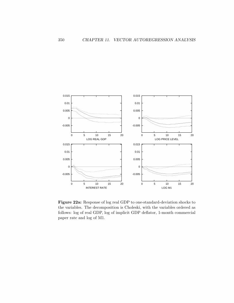
350 CHAPTER 11. VECTOR AUTOREGRESSION ANALYSIS
-0.005
0
0.005
0.01
0.015
0 5 10 15 20
LOG REAL GDP
-0.005
0
0.005
0.01
0.015
0 5 10 15 20
LOG PRICE LEVEL
-0.005
0
0.005
0.01
0.015
0 5 10 15 20
INTEREST RATE
-0.005
0
0.005
0.01
0.015
0 5 10 15 20
LOG M1
Figure 22a: Response of log real GDP to one-standard-deviation shocks tothe variables. The decomposition is Choleski, with the variables ordered asfollows: log of real GDP, log of implicit GDP deflator, 1-month commercialpaper rate and log of M1.
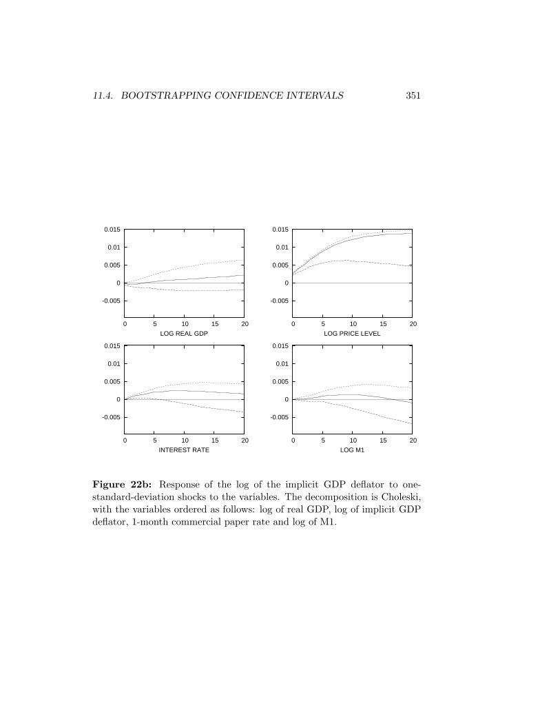
11.4. BOOTSTRAPPING CONFIDENCE INTERVALS 351
-0.005
0
0.005
0.01
0.015
0 5 10 15 20
LOG REAL GDP
-0.005
0
0.005
0.01
0.015
0 5 10 15 20
LOG PRICE LEVEL
-0.005
0
0.005
0.01
0.015
0 5 10 15 20
INTEREST RATE
-0.005
0
0.005
0.01
0.015
0 5 10 15 20
LOG M1
Figure 22b: Response of the log of the implicit GDP deflator to one-standard-deviation shocks to the variables. The decomposition is Choleski,with the variables ordered as follows: log of real GDP, log of implicit GDPdeflator, 1-month commercial paper rate and log of M1.

352 CHAPTER 11. VECTOR AUTOREGRESSION ANALYSIS
-0.005
0
0.005
0.01
0.015
0 5 10 15 20
LOG REAL GDP
-0.005
0
0.005
0.01
0.015
0 5 10 15 20
LOG PRICE LEVEL
-0.005
0
0.005
0.01
0.015
0 5 10 15 20
INTEREST RATE
-0.005
0
0.005
0.01
0.015
0 5 10 15 20
LOG M1
Figure 22c: Response of the 1-month commercial paper rate to one-standard-deviation shocks to the variables. The decomposition is Choleskiwith the variables ordered as follows: log of real GDP, log of implicit GDPdeflator, 1-month commercial paper rate and log of M1.
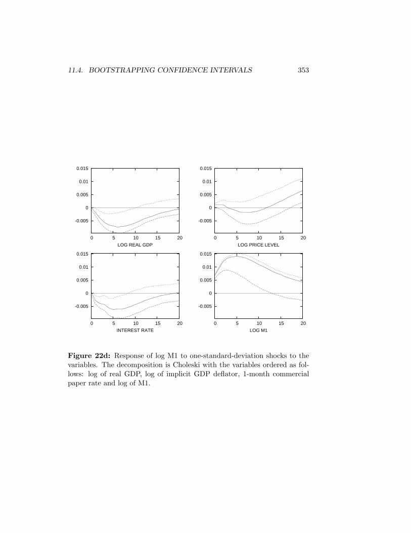
11.4. BOOTSTRAPPING CONFIDENCE INTERVALS 353
-0.005
0
0.005
0.01
0.015
0 5 10 15 20
LOG REAL GDP
-0.005
0
0.005
0.01
0.015
0 5 10 15 20
LOG PRICE LEVEL
-0.005
0
0.005
0.01
0.015
0 5 10 15 20
INTEREST RATE
-0.005
0
0.005
0.01
0.015
0 5 10 15 20
LOG M1
Figure 22d: Response of log M1 to one-standard-deviation shocks to thevariables. The decomposition is Choleski with the variables ordered as fol-lows: log of real GDP, log of implicit GDP deflator, 1-month commercialpaper rate and log of M1.

354 CHAPTER 11. VECTOR AUTOREGRESSION ANALYSIS
For bootstrapped estimation of structural VARs I have constructed thefunction VAR-estimate-structural. As in the case of VAR-estimate-choleski, by setting the number of bootstrap runs equal to zero, the functioncan also be used to simply estimate the VAR without bootstrapping. TheVAR-estimate-structural function takes twelve arguments which mustappear in the following order:
1. The list of variables.
2. The number of lags.
3. A list of the names of the variables.
4. An indicator variable equal to 1 if the system is over-identified and 0if it is just-identified.
5. An indicator variable equal to 0 if the newtonmax function is to beused in over-identified estimation and equal to 1 if the nelmeadmaxfunction is to be used.
6. The datelist to which the variables must all conform (this will be longerthan the interval over which the VAR will be run to accommodate lagsof the variables).
7. The beginning date of the VAR.
8. The ending date of the VAR.
9. The number of steps for the impulse-responses and forecast-error-variance decompositions.
10. An indicator variable equal 1 if the impulse-responses and forecast-error-variance decompositions are to be written to the screen and zerootherwise.
11. An indicator variable equal to 1 if the impulse-responses are to beplotted to the screen and zero otherwise.
12. The number of bootstrap runs.
As in the case of the VAR-estimate-choleski function, which takes allthe arguments above except 4) and 5), when the number of bootstrap runsexceeds zero the indicator variables specified in 10) and 11) are automati-cally set equal to zero, regardless of what is entered on the command line.
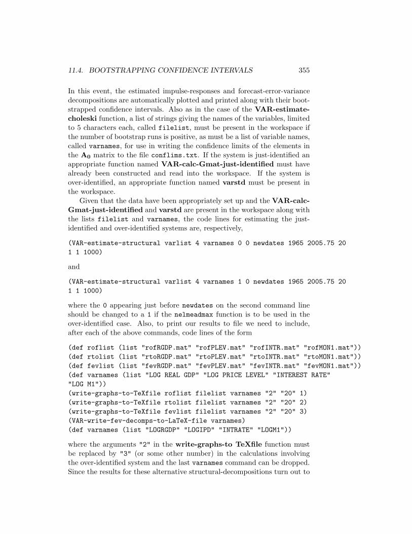
11.4. BOOTSTRAPPING CONFIDENCE INTERVALS 355
In this event, the estimated impulse-responses and forecast-error-variancedecompositions are automatically plotted and printed along with their boot-strapped confidence intervals. Also as in the case of the VAR-estimate-choleski function, a list of strings giving the names of the variables, limitedto 5 characters each, called filelist, must be present in the workspace ifthe number of bootstrap runs is positive, as must be a list of variable names,called varnames, for use in writing the confidence limits of the elements inthe A0 matrix to the file conflims.txt. If the system is just-identified anappropriate function named VAR-calc-Gmat-just-identified must havealready been constructed and read into the workspace. If the system isover-identified, an appropriate function named varstd must be present inthe workspace.
Given that the data have been appropriately set up and the VAR-calc-Gmat-just-identified and varstd are present in the workspace along withthe lists filelist and varnames, the code lines for estimating the just-identified and over-identified systems are, respectively,
(VAR-estimate-structural varlist 4 varnames 0 0 newdates 1965 2005.75 201 1 1000)
and
(VAR-estimate-structural varlist 4 varnames 1 0 newdates 1965 2005.75 201 1 1000)
where the 0 appearing just before newdates on the second command lineshould be changed to a 1 if the nelmeadmax function is to be used in theover-identified case. Also, to print our results to file we need to include,after each of the above commands, code lines of the form
(def roflist (list "rofRGDP.mat" "rofPLEV.mat" "rofINTR.mat" "rofMON1.mat"))(def rtolist (list "rtoRGDP.mat" "rtoPLEV.mat" "rtoINTR.mat" "rtoMON1.mat"))(def fevlist (list "fevRGDP.mat" "fevPLEV.mat" "fevINTR.mat" "fevMON1.mat"))(def varnames (list "LOG REAL GDP" "LOG PRICE LEVEL" "INTEREST RATE""LOG M1"))(write-graphs-to-TeXfile roflist filelist varnames "2" "20" 1)(write-graphs-to-TeXfile rtolist filelist varnames "2" "20" 2)(write-graphs-to-TeXfile fevlist filelist varnames "2" "20" 3)(VAR-write-fev-decomps-to-LaTeX-file varnames)(def varnames (list "LOGRGDP" "LOGIPD" "INTRATE" "LOGM1"))
where the arguments "2" in the write-graphs-to TeXfile function mustbe replaced by "3" (or some other number) in the calculations involvingthe over-identified system and the last varnames command can be dropped.Since the results for these alternative structural-decompositions turn out to
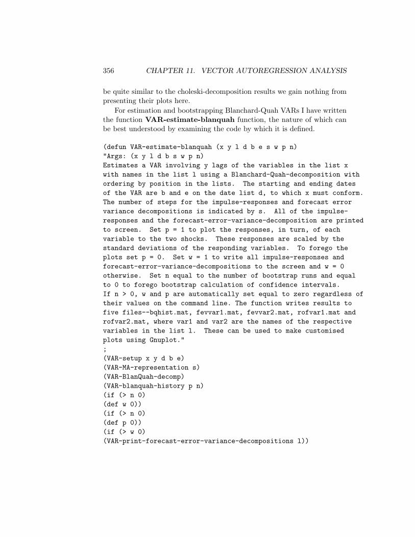
356 CHAPTER 11. VECTOR AUTOREGRESSION ANALYSIS
be quite similar to the choleski-decomposition results we gain nothing frompresenting their plots here.
For estimation and bootstrapping Blanchard-Quah VARs I have writtenthe function VAR-estimate-blanquah function, the nature of which canbe best understood by examining the code by which it is defined.
(defun VAR-estimate-blanquah (x y l d b e s w p n)"Args: (x y l d b s w p n)Estimates a VAR involving y lags of the variables in the list xwith names in the list l using a Blanchard-Quah-decomposition withordering by position in the lists. The starting and ending datesof the VAR are b and e on the date list d, to which x must conform.The number of steps for the impulse-responses and forecast errorvariance decompositions is indicated by s. All of the impulse-responses and the forecast-error-variance-decomposition are printedto screen. Set p = 1 to plot the responses, in turn, of eachvariable to the two shocks. These responses are scaled by thestandard deviations of the responding variables. To forego theplots set p = 0. Set w = 1 to write all impulse-responses andforecast-error-variance-decompositions to the screen and w = 0otherwise. Set n equal to the number of bootstrap runs and equalto 0 to forego bootstrap calculation of confidence intervals.If n > 0, w and p are automatically set equal to zero regardless oftheir values on the command line. The function writes results tofive files--bqhist.mat, fevvar1.mat, fevvar2.mat, rofvar1.mat androfvar2.mat, where var1 and var2 are the names of the respectivevariables in the list l. These can be used to make customisedplots using Gnuplot.";(VAR-setup x y d b e)(VAR-MA-representation s)(VAR-BlanQuah-decomp)(VAR-blanquah-history p n)(if (> n 0)(def w 0))(if (> n 0)(def p 0))(if (> w 0)(VAR-print-forecast-error-variance-decompositions l))
11.4. BOOTSTRAPPING CONFIDENCE INTERVALS 357
(if (> w 0)(VAR-print-impulse-responses l))(if (> p 0)(VAR-plot-impulse-responses-of l))(if (> n 0)(def rtoout (VAR-results-vectors rtomats)))(if (> n 0)(def rofout (VAR-results-vectors rofmats)))(if (> n 0)(def fevout (VAR-results-vectors fevmats)))(if (> n 0)(dotimes (v n)(terpri)(princ "Bootstrap Run Number ")(princ v)(terpri)(VAR-bootstrap-values)(VAR-MA-representation s)(VAR-BlanQuah-decomp)(def rtoout (VAR-add-results-vectors rtomats rtoout))(def rofout (VAR-add-results-vectors rofmats rofout))(def fevout (VAR-add-results-vectors fevmats fevout)))) ; end dotimes v(if (> n 0)(def climrto (VAR-calc-conf-limits rtoout)))(if (> n 0)(def climrof (VAR-calc-conf-limits rofout)))(if (> n 0)(def climfev (VAR-calc-conf-limits fevout)))(if (> n 0)(VAR-plot-conf-limits climrof 1))(if (> n 0)(VAR-plot-conf-limits climfev 3))(if (> n 0)(VAR-write-conf-limits-to-file climrof 1))(if (> n 0)(VAR-write-conf-limits-to-file climfev 3));) ; end of function
358 CHAPTER 11. VECTOR AUTOREGRESSION ANALYSIS
A careful examination will reveal that this function differs from the VAR-estimate-choleski and VAR-estimate-structural functions only in mi-nor details. In our Canada/U.S. real exchange rate VAR, the function writesfive files—bqhist.mat, fevrexch.mat, fevnexch.mat, rofrexch.mat androfnexch.mat which I have used to make, using Gnuplot, the customisedplots in Figure 23. To do this I created eight Gnuplot files, rofn2m.plt,rofn2r.plt, rofr2m, rofr2r.plt, fevn2m.plt, fevn2r.plt, fevr2m, andfevr2r.plt and the LATEX file stmlspf23.tex. These files are providedalong with this document for use as templates for use in analyses of othercountries’ real and nominal exchange rates. With minor modifications, theycan also be adapted to Blanchard-Quah VARs that do not involve real andnominal exchange rates.
After the data have been prepared, as was done above, our Blanchard-Quah real and nominal exchange rate VAR can be run using the followingcode.
(def varlist (list drex dnex))(def filelist (list "rexch" "nexch"))(def lablist (list "real exch rate" "nom exch rate"))(def shocklist (list "mon shk" "real shk"))(def histlabs (list "real exch rate (pts) and money shocks""real exch rate (pts) and real shocks""nom exch rate (pts) money shocks" "nom exch rate (pts) and real shocks"))(VAR-estimate-blanquah varlist 18 lablist difdates 1974.0 2005.9166 201 1 1000)
The impulse-responses and forecast-error-variance-decompositions are plot-ted in Figure 23. The historical decompositions were plotted in Figure21. The LATEX file stmlspf21.tex and the two Gnuplot files histnca.pltand histrca.plt used to create those plots are also provided along withthis document as templates. These Gnuplot files referenced the data filebqhistca.mat which is simply the file bqhist.mat renamed. That file wasproduced by the function VAR-blanquah-history which was called by theVAR-estimate-blanquah function above.
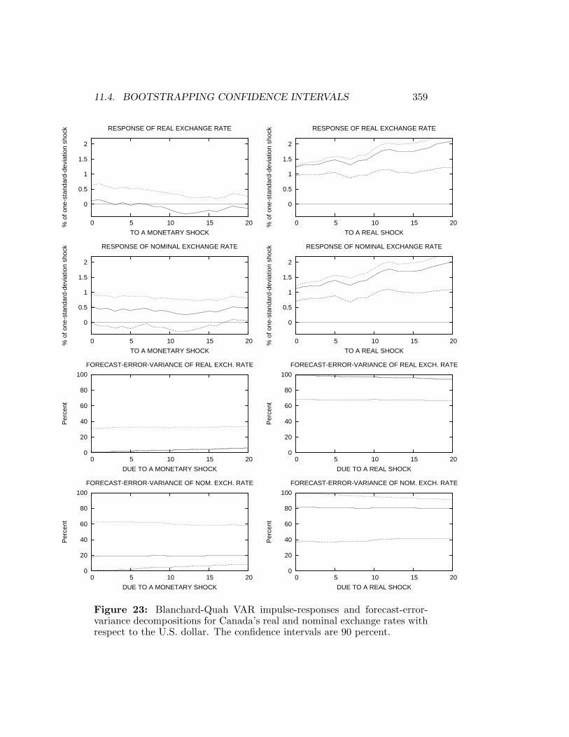
11.4. BOOTSTRAPPING CONFIDENCE INTERVALS 359
0
0.5
1
1.5
2
0 5 10 15 20% o
f one
-sta
ndar
d-de
viat
ion
shoc
k
TO A MONETARY SHOCK
RESPONSE OF REAL EXCHANGE RATE
0
0.5
1
1.5
2
0 5 10 15 20% o
f one
-sta
ndar
d-de
viat
ion
shoc
k
TO A REAL SHOCK
RESPONSE OF REAL EXCHANGE RATE
0
0.5
1
1.5
2
0 5 10 15 20% o
f one
-sta
ndar
d-de
viat
ion
shoc
k
TO A MONETARY SHOCK
RESPONSE OF NOMINAL EXCHANGE RATE
0
0.5
1
1.5
2
0 5 10 15 20% o
f one
-sta
ndar
d-de
viat
ion
shoc
k
TO A REAL SHOCK
RESPONSE OF NOMINAL EXCHANGE RATE
0
20
40
60
80
100
0 5 10 15 20
Per
cent
DUE TO A MONETARY SHOCK
FORECAST-ERROR-VARIANCE OF REAL EXCH. RATE
0
20
40
60
80
100
0 5 10 15 20
Per
cent
DUE TO A REAL SHOCK
FORECAST-ERROR-VARIANCE OF REAL EXCH. RATE
0
20
40
60
80
100
0 5 10 15 20
Per
cent
DUE TO A MONETARY SHOCK
FORECAST-ERROR-VARIANCE OF NOM. EXCH. RATE
0
20
40
60
80
100
0 5 10 15 20
Per
cent
DUE TO A REAL SHOCK
FORECAST-ERROR-VARIANCE OF NOM. EXCH. RATE
Figure 23: Blanchard-Quah VAR impulse-responses and forecast-error-variance decompositions for Canada’s real and nominal exchange rates withrespect to the U.S. dollar. The confidence intervals are 90 percent.

360 CHAPTER 11. VECTOR AUTOREGRESSION ANALYSIS

Chapter 12
Forecasting
Our final topic deals with econometric issues involved in forecasting eco-nomic time-series. Time-series forecasts must deal with the fact that theunderlying models on which forecasts are based inevitably change throughtime in a wide variety of dimensions as changes in the economic structureand economic policy occur and as agents learn about the magnitudes ofthose changes. In analytical work directed toward understanding how theeconomy functions, we often use pseudo-forecasts—that is, forecasts of pasteconomic changes whose results are now known—to model how agents mayhave predicted and reacted to those events. A good example is the problemof constructing an unanticipated money shock series to use in analysing thehistorical effects of unanticipated money shocks on interest rates, exchangerates, etc. Most of what follows deals with this type of forecast althoughsome minimal effort will be devoted to actually forecasting future, as yet un-known, levels of time-series. We begin with the crudest of forecasts—simpletrend projection.
12.1 Trend Projections
For making trend projections I wrote the function OLS-trend-projectionwhich takes the following five arguments in order—the series being projected,the datelist to which it conforms, the number of observations over which thetrend is to be calculated, the date of the first forecasted value, and thenumber of subsequent values to be forecasted. The function leaves a list ofthe predicted values, called predvals in the workspace. Using the USM1SAvariable in the data file causdat.lsp we illustrate by making a 12-monthprojection, starting at the beginning of 2005. We take the logarithm of
361

362 CHAPTER 12. FORECASTING
the M1 series, multiply it by 100 and then subtract the level of the firstobservation of the resulting series from all observations, thereby expressingeach period’s value as, roughly, the percent increase from January 1962. Thepredicted and actual values of the series from the beginning of 2000 onwardare plotted to the screen and written to file for plotting below as Figure 24using Gnuplot.
200
205
210
215
220
225
230
235
2000 2001 2002 2003 2004 2005 2006
Per
cent
age
Incr
ease
Sin
ce J
anua
ry 1
962
ActualForecasted
Figure 24: Actual and forecasted values of United States M1 for the year2005 based on a trend projection of 2004 levels.
> (load "causdat"); loading causdat.lspT> (load "addfuncs"); loading addfuncs.lspT> (variables)(CAUSNPR CAUSREX DATESMO DATESQ USCPAPR USCPI USCURR USEXB USFFR USIPDUSM1SA USM2SA USMBADJ USNBREXB USNBRSA USNGDP USRGDP USTRARR)> (def logm1 (* 100 (log usm1sa)))LOGM1> (def m1 (- logm1 (select logm1 0)))M1> (OLS-trend-projection m1 datesmo 12 2005.0 12)(225.29081744341556 225.7078925933587 226.12496774330185 226.542042893245226.95911804318814 227.37619319313131 227.79326834307446 228.2103434930176228.62741864296075 229.0444937929039 229.46156894284704 229.87864409279018)

12.1. TREND PROJECTIONS 363
> (def newm1 (remove-last 12 m1))NEWM1> (def newm1 (append newm1 predvals))NEWM1> (date2obs datesmo 2000.0)456> (def plotdates (- (remove-first 455 datesmo) 1900))PLOTDATES> (def plot1 (plot-lines plotdates (remove-first 455 m1)))PLOT1> (send plot1 :add-lines plotdates (remove-first 455 newm1))NIL> (write-matrix-to-file (bind-columns (remove-first 455 datesmo)(remove-first 455 m1)(remove-first 455 newm1)) "stmlspf24.mat")T
The forecast is terrible! For purposes of calculating the unanticipated moneyshock we need to make a running one-period ahead forecast. This can bedone using my function running-trend-projection, which takes, in or-der, the following five arguments—the series being projected, the datelistto which it conforms, the number of periods over which the trend is to becalculated, and the first and last periods forecasted, respectively. The re-sulting series, plotted in the bottom panel of Figure 25, and some usefulinformation about it is calculated using the following code, where runningfour-month trends are projected.
(running-trend-projection m1 datesmo 4 2000.0 2005.917)(def uasm1 (* 100 (/ (- actlist predlist) predlist)))(def msqfe (mean (/ (inner-product uasm1 uasm1)(length predlist))))(mean uasm1)(standard-deviation uasm1)(sqrt msqfe)
The mean of the unanticipated money shocks, taken as percentages of pre-dicted levels, is -0.015 for the period 2000-2005 and the standard-deviationis 0.453. The root-mean-square-forecast-error is 0.450. One will, of course,get a different measure of the unanticipated money shock for each possibleperiod-length over which the trend is estimated. And the ‘best length’ forany given period can only be known after the data for that period becomeavailable.

364 CHAPTER 12. FORECASTING
200
205
210
215
220
225
230
2000 2001 2002 2003 2004 2005 2006
ACTUAL AND PREDICTED M1 AS PERCENTAGES OF JANUARY 1962 LEVELS
ActualPredicted
-2.5
-2
-1.5
-1
-0.5
0
0.5
1
1.5
2
2000 2001 2002 2003 2004 2005 2006
UNANTICIPATED M1 SHOCKS AS PERCENTAGES OF PREDICTED LEVELS
Figure 25: Actual and predicted values of United States M1, and theimplied unanticipated M1 shocks, for the years 2000-2005, based on runningone-period trend projections of values for the previous four months.
A better method of estimating past anticipated M1 levels and forecastingit, or any other variable, in future periods would undoubtedly be to use OLSpredictions based not only on past data for the variable in question butpast data for other variables that are related to it. Such methods will beexplored later after we have dealt with more sophisticated ways of forecastingvariables using only their own past values.

12.2. ARIMA FORECASTS 365
12.2 ARIMA Forecasts
Autoregressive-integrated-moving-average time-series processes are conven-tionally expressed in the form ARIMA(p, d, q) where p is the number ofautoregressive lags, q is the number of moving average lags, and d is thenumber of times the series has to be differenced to produce a stationaryARMA(p, q) process.1
The first step in fitting an ARIMA process to our log U.S. M1 seriesis therefore to determine how many times the series must be differencedto make it stationary. Using the ppunit function, we obtain the followingresults.
PHILLIPS-PERRON TEST --- log USM1Lags Truncated at 1
Least Squares Estimates:
Constant 6.295173E-2 (0.250127)Trend -1.872048E-3 (9.996069E-4)Lagged Y 1.00298 (2.044931E-3)
R Squared: 0.999945Sigma hat: 0.553965Number of cases: 527Degrees of freedom: 524
Standard t-ratios:
Constant 0.2516791340876413Trend -1.8727836646422076Lagged Y = 0 490.47205571099784Lagged Y = 1 1.4579733047692311
1A useful discussion of the basics of this type of time-series modelling can be found inChapter 2 of the Enders book cited earlier.

366 CHAPTER 12. FORECASTING
Least Squares Estimates:
Constant 0.523269 (4.646994E-2)Lagged Y 0.999200 (3.252681E-4)
R Squared: 0.999944Sigma hat: 0.555286Number of cases: 527Degrees of freedom: 525
Standard t-ratios:
Constant 11.260379994808872Lagged Y = 0 3071.927789348678Lagged Y = 1 -2.4586942404249337
Least Squares Estimates:
Lagged Y 1.00233 (1.884707E-4)
R Squared: 0.999931Sigma hat: 0.618130Number of cases: 527Degrees of freedom: 526
Standard t-ratios:
Lagged Y = 0 5318.214607984291Lagged Y = 1 12.349961865121243
PP t-ratio for Coefficient of Lagged Y = 1:1.1405659035390487
PP t-ratio for Constant = 0:0.3605409345990346
PP t-ratio for Trend Coefficient = 0:-1.3860482568827504

12.2. ARIMA FORECASTS 367
PP Statistic for Coefficients of Trend = 0 and Lagged Y = 1:3.7300002111992048
PP t-ratio for Coefficient of Lagged Y = 1 in regression without trend:-2.1749722067422996
PP t-ratio for Coefficient of Lagged Y = 1 in regression withneither constant nor trend:
10.260606203027326
PHILLIPS-PERRON TEST --- log USM1Lags Truncated at 5
Least Squares Estimates:
Constant 6.295173E-2 (0.250127)Trend -1.872048E-3 (9.996069E-4)Lagged Y 1.00298 (2.044931E-3)
R Squared: 0.999945Sigma hat: 0.553965Number of cases: 527Degrees of freedom: 524
Standard t-ratios:
Constant 0.2516791340876413Trend -1.8727836646422076Lagged Y = 0 490.47205571099784Lagged Y = 1 1.4579733047692311
Least Squares Estimates:
Constant 0.523269 (4.646994E-2)Lagged Y 0.999200 (3.252681E-4)
R Squared: 0.999944Sigma hat: 0.555286
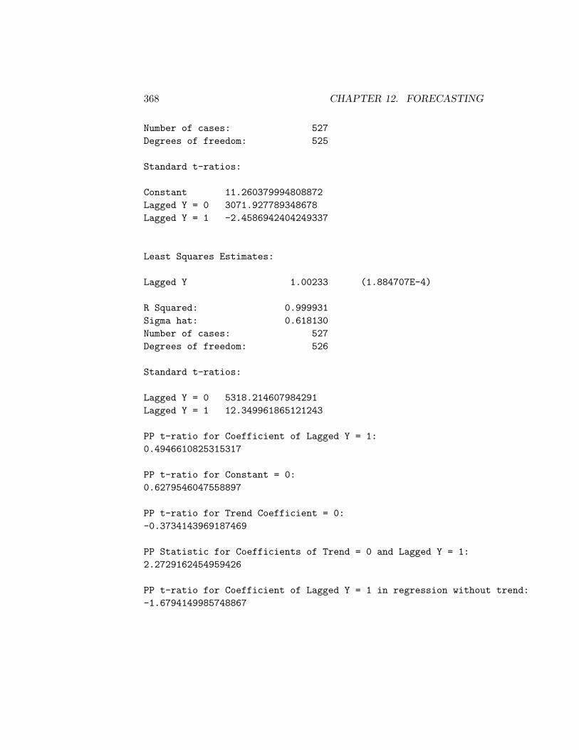
368 CHAPTER 12. FORECASTING
Number of cases: 527Degrees of freedom: 525
Standard t-ratios:
Constant 11.260379994808872Lagged Y = 0 3071.927789348678Lagged Y = 1 -2.4586942404249337
Least Squares Estimates:
Lagged Y 1.00233 (1.884707E-4)
R Squared: 0.999931Sigma hat: 0.618130Number of cases: 527Degrees of freedom: 526
Standard t-ratios:
Lagged Y = 0 5318.214607984291Lagged Y = 1 12.349961865121243
PP t-ratio for Coefficient of Lagged Y = 1:0.4946610825315317
PP t-ratio for Constant = 0:0.6279546047558897
PP t-ratio for Trend Coefficient = 0:-0.3734143969187469
PP Statistic for Coefficients of Trend = 0 and Lagged Y = 1:2.2729162454959426
PP t-ratio for Coefficient of Lagged Y = 1 in regression without trend:-1.6794149985748867

12.2. ARIMA FORECASTS 369
PP t-ratio for Coefficient of Lagged Y = 1 in regression withneither constant nor trend:
6.965254218198062
PHILLIPS-PERRON TEST --- 1st Diff log USM1Lags Truncated at 1
Least Squares Estimates:
Constant 0.293864 (2.912671E-2)Trend -3.087277E-4 (1.527266E-4)Lagged Y 0.309200 (4.166748E-2)
R Squared: 0.108078Sigma hat: 0.528428Number of cases: 526Degrees of freedom: 523
Standard t-ratios:
Constant 10.089148962701483Trend -2.0214398420996815Lagged Y = 0 7.420648629463743Lagged Y = 1 -16.578882593019177
Least Squares Estimates:
Constant 0.289623 (2.913648E-2)Lagged Y 0.318760 (4.151993E-2)
R Squared: 0.101109Sigma hat: 0.529982Number of cases: 526Degrees of freedom: 524

370 CHAPTER 12. FORECASTING
Standard t-ratios:
Constant 9.940216334967369Lagged Y = 0 7.677283110910276Lagged Y = 1 -16.407538489571188
Least Squares Estimates:
Lagged Y 0.570139 (3.586619E-2)
R Squared: 0.000000Sigma hat: 0.577243Number of cases: 526Degrees of freedom: 525
Standard t-ratios:
Lagged Y = 0 15.896288611793661Lagged Y = 1 -11.985120756173018
PP t-ratio for Coefficient of Lagged Y = 1:-16.420430011935018
PP t-ratio for Constant = 0:9.990662040856604
PP t-ratio for Trend Coefficient = 0:-3.0707337906872296
PP Statistic for Coefficients of Trend = 0 and Lagged Y = 1:134.9307485061046
PP t-ratio for Coefficient of Lagged Y = 1 in regression without trend:-16.24219008759896
PP t-ratio for Coefficient of Lagged Y = 1 in regression withneither constant nor trend:
-10.866713564263971

12.2. ARIMA FORECASTS 371
PHILLIPS-PERRON TEST --- 1st Diff log USM1Lags Truncated at 5
Least Squares Estimates:
Constant 0.293864 (2.912671E-2)Trend -3.087277E-4 (1.527266E-4)Lagged Y 0.309200 (4.166748E-2)
R Squared: 0.108078Sigma hat: 0.528428Number of cases: 526Degrees of freedom: 523
Standard t-ratios:
Constant 10.089148962701483Trend -2.0214398420996815Lagged Y = 0 7.420648629463743Lagged Y = 1 -16.578882593019177
Least Squares Estimates:
Constant 0.289623 (2.913648E-2)Lagged Y 0.318760 (4.151993E-2)
R Squared: 0.101109Sigma hat: 0.529982Number of cases: 526Degrees of freedom: 524
Standard t-ratios:
Constant 9.940216334967369Lagged Y = 0 7.677283110910276Lagged Y = 1 -16.407538489571188
372 CHAPTER 12. FORECASTING
Least Squares Estimates:
Lagged Y 0.570139 (3.586619E-2)
R Squared: 0.000000Sigma hat: 0.577243Number of cases: 526Degrees of freedom: 525
Standard t-ratios:
Lagged Y = 0 15.896288611793661Lagged Y = 1 -11.985120756173018
PP t-ratio for Coefficient of Lagged Y = 1:-17.472082294840195
PP t-ratio for Constant = 0:10.641817495663703
PP t-ratio for Trend Coefficient = 0:2.5945726259447213
PP Statistic for Coefficients of Trend = 0 and Lagged Y = 1:152.34439146210102
PP t-ratio for Coefficient of Lagged Y = 1 in regression without trend:-17.328491466577574
PP t-ratio for Coefficient of Lagged Y = 1 in regression withneither constant nor trend:
-12.836201904905057
From a comparison of the above statistics with the critical values in thefirst table in our Statistical Tables, it is clear that the null-hypothesis ofnon-stationarity cannot be rejected for the logarithm of U.S. M1 but thefirst-difference of this series is unquestionably stationary.
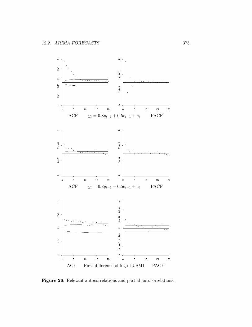
12.2. ARIMA FORECASTS 373
ACF yt = 0.8yt−1 + 0.5et−1 + et PACF
ACF yt = 0.8yt−1 − 0.5et−1 + et PACF
ACF First-difference of log of USM1 PACF
Figure 26: Relevant autocorrelations and partial autocorrelations.

374 CHAPTER 12. FORECASTING
The question then is how to decide upon the values of p and q to usein fitting an ARMA(p, q) process to the first-difference of the series. Thetop two panels in Figure 26 give the autocorrelations and partial autocorre-lations of specially constructed ARMA(1,1) series using a function I wrotecalled create-ARMA-series which takes two arguments—first, the lengthof the series and second, the number of lags of the autocorrelation and par-tial autocorrelation functions to print. The function also requires that twolists be in the workspace, a list of the AR coefficients called arlist and alist of the MA coefficients called malist. An AR or MA process can be con-structed by simply setting the coefficient of a single MA or AR lag to be zero.As noted by Enders, the autocorrelation function begins declining at lag qwhen p > 0 and the partial autocorrelation function begins declining at lag pwhen q > 0. If q = 0 (there being no moving average terms) and p = 1 (oneautoregressive lag) the autocorrelation function will decline continuouslywhen the coefficient of autoregressive term is positive. If that coefficient isnegative, the autocorrelation function will decline in absolute value but theautocorrelations will alternatively take negative and positive values. Thepartial autocorrelation function will consist of a single spike at lag 1. Al-ternatively, if p = 0 (no autoregressive lags) and q = 1 (one moving-averagelag) there will be a single spike at lag 1 in the autocorrelation function andthe partial autocorrelation function will decline continuously to thereafterin absolute value, with the first partial-autocorrelation being negative andthe subsequent partial-autocorrelations alternating in sign if the coefficientof the lagged error term is positive, and all partial-autocorrelations beingpositive if that coefficient is negative. When p > 1 the damping of thepartial autocorrelation function will begin after p lags and when q > 1 theautocorrelation function will begin to damp after q lags. As is clear fromthe top two panels, when both the autocorrelations and partial autocorre-lations are declining, p and q must both be greater than or equal to unity.It would therefore appear from the bottom panel of Figure 26 that there isperhaps one autoregressive lag and one or more moving-average lags withthe coefficient of the autoregressive lag being positive and that of the firstmoving-average lag being negative.
I have written three functions to fit these processes to data. But first,to set the exact time-period over which the process is to be fit to the se-ries, we have to call my ARMA-set-data function which takes as its fivearguments, in order, the name of the series, the datelist to which it con-forms, the maximum number of autoregressive lags, the beginning date forthe fitted process and the ending date. This function returns the series listnewy to be used in subsequent estimation and leaves both this list and a

12.2. ARIMA FORECASTS 375
new datelist called newdates in the workspace. To fit an AR process we usemy AR-estimate, which takes as its two arguments, the name of the seriesto which the process is being fitted and then the number of AR lags.
The batch code for the calculations underlying Figure 26, together withan AR(2) fit, is presented below along with the results.
(load "addfuncs")(load "maximize")(load "causdat");(def arlist (list 0.8))(def malist (list 0.5))(create-ARMA-series 1100 20);(def malist (list -0.5))(create-ARMA-series 1100 20);(def logm1 (* 100 (log usm1sa)))(def m1 (- logm1 (select logm1 0)));(ppunit m1 "log USM1" 1)(ppunit m1 "log USM1" 5);(def dm1 (difference m1));(ppunit dm1 "1st Diff log USM1" 1)(ppunit dm1 "1st Diff log USM1" 5);(def datesmo (remove-first-element datesmo))(ARMA-setdata dm1 dates 2 1974.0 2004.917)(acf newy 20 "ACF")(pacf newy 20 "PACF");(AR-estimate newy 2)
376 CHAPTER 12. FORECASTING
Estimation of AR Process:
Coefficient Std. Error T-Statistic P-Value
Constant 0.242 0.040 6.031 0.000AR(1) 0.259 0.051 5.069 0.000AR(2) 0.194 0.051 3.794 0.000
Sum of Squared Residuals = 123.81360386796065
Degrees of Freedom = 369
AIC = 1798.5851333028083SBC = 1810.3418148656278
Ljung-Box Q-statistics:LAG Q DF Pval4 6.703 1 0.0105 10.366 2 0.0066 14.699 3 0.0027 16.936 4 0.0028 21.492 5 0.001
.............................
.............................
.............................
89 104.945 86 0.08190 104.948 87 0.09291 105.315 88 0.10192 106.770 89 0.09793 108.298 90 0.092
It turns out that both lags are statistically significant, but the Ljung-Box Q-statistics indicate very substantial serial correlation remaining in the resid-uals.
For fitting MA processes, we use my MA-estimate function which takesas its three arguments, in order, the series to which the process is beingfitted, a guess list giving values of the parameters at which the maximum-

12.2. ARIMA FORECASTS 377
likelihood estimation is to start, and an indicator argument taking a value of0 if the newtonmax function is to be used and a value of 1 if the nelmeadmaxfunction is to be used. The parameter list is ordered as follows—constant,MA coefficient 1, MA coefficient 2, ....., true variance of residuals. When thenelmeadmax function is used there must be present in the workspace a listcalled sizelist giving each dimension of the initial simplex. For this list,I have gotten by using a list of 1’s or 0.5’s containing the same number ofelements as the number of parameters. One should always start by using thenewtonmax function, turning to the nelmeadmax function when a maximumcannot be found using newtonmax. If nelmeadmax yields silly results, likeimaginary numbers for standard-errors, the coefficients it produces shouldthen be used as the guess-list for using newtonmax. The batch code forfitting an MA(2) process to our series is as follows.
(def gueslist (list 0.5 0.5 0.5 1))(MA-estimate newy gueslist 0)(def sizelist (list .5 .5 .5 .5))(MA-estimate newy gueslist 1)(def gueslist (list 0.425 0.233 0.152 0.280))(MA-estimate newy gueslist 0)
Estimation was started using newtonmax. Since the results contained non-sense, sizelist was created and nelmeadmax was used. Given that thelatter function was unable to yield proper standard errors, the results itproduced were layed out in a new version of gueslist and the newtonmaxfunction was then successfully applied. I have written an additional functioncalled MA-residuals, that lurks in the background, to calculate the resid-uals for each MA representation of the series list to which the MA processis being fitted. The MA-estimate function calls this function repeatedlyin the course of attempting to find a maximum of the likelihood function.2
The results we end up with are
Estimation of MA Process:
maximizing...Iteration 0.Criterion value = -335.781Iteration 1.Criterion value = -331.659
2For background, see pages 127-134 of the textbook by Hamilton that was cited earlier.

378 CHAPTER 12. FORECASTING
Iteration 2.Criterion value = -331.301Iteration 3.Criterion value = -331.296Iteration 4.Criterion value = -331.296Reason for termination: gradient size is less than gradient tolerance.
Coefficient Std. Error T-statConstant 0.446 0.038 11.765Lag 1 0.236 0.047 5.040Lag 2 0.164 0.043 3.783Variance 0.344 0.017
Sum of Squared Residuals = 128.76861148372393
Degrees of Freedom = 371
AIC = 1822.8983895319911SBC = 1834.6711569242348
Ljung-Box Q-statistics:LAG Q DF Pval4 24.333 1 0.0005 32.401 2 0.0006 42.305 3 0.0007 48.848 4 0.0008 57.962 5 0.000
.............................
.............................
.............................
92 168.029 89 0.00093 169.549 90 0.00094 170.236 91 0.000
While both MA lags are statistically significant, the fitted residuals againcontain very high serial correlation.

12.2. ARIMA FORECASTS 379
Finally, we fit ARMA(1,1) and ARMA(1,2) processes to our series usingthe ARMA-estimate function I wrote for the purpose. This function takessix arguments in the following order—the series to which the process is beingfitted, the number of autoregressive lags, the number of moving average lags,a list of initial guesses as to the magnitudes of the parameters, the integer1 if a constant term is to be included or, alternatively, a 0 if no constantis to be included, and finally, a zero if the newtonmax function is to beused or the integer 1 if the nelmeadmax function is to be used. The initial-guess parameter list, of length p + q + c + 1, where c = 1 if a constant isto be included and c = 0 otherwise, must be ordered as follows—constant(if c = 1), AR coefficient 1, AR coefficient 2, ........, MA coefficient 1, MAcoefficient 2, ....., true variance of residuals. Again, if nelmeadmax is usedthere must be a list called sizelist already in the workspace containing oneelement for each element in the initial-guess parameter list. As in the casewhere MA processes are being fitted to a series, I have written a function thatremains in the background for the ARMA-estimate function to use. It iscalled ARMA-residuals and calculates the residuals for a particular set ofARMA parameters that the newtonmax or nelmeadmax will then calculatethe likelihood of during the maximisation process.3 The batch code forfitting ARMA(1,1) and ARMA(2,2) processes to the first-difference of logUnited States M1 is as follows.
(def gueslist (list 0.5 0.5 0.5 1))(ARMA-estimate (remove-first-element newy) 1 1 gueslist 1 0)(def sizelist (list 1 1 1 1))(ARMA-estimate (remove-first-element newy) 1 1 gueslist 1 1)(def gueslist (list 0.022 0.940 -0.780 0.253))(ARMA-estimate (remove-first-element newy) 1 1 gueslist 1 0)(def gueslist (list 0.022 0.940 -0.780 0 0.253))(ARMA-estimate (remove-first-element newy) 1 2 gueslist 1 0)
We first attempt to fit an ARMA(1,1) process using the newtonmax function.When that fails, we define sizelist and proceed to use the nelmeadmaxfunction. The results from that estimation are then fed as gueslist tothe newtonmax function. Then an ARMA(1,2) process is fit to the seriesusing the previous gueslist with a zero inserted as an initial guess for thesecond MA coefficient. In all these estimates we remove the first element ofnewy to make the series identical to the one to which the AR(2) process waspreviously fit so that when we compare the AIC and SBC statistics they
3See again the pages from the Hamilton book cited in the previous footnote.
380 CHAPTER 12. FORECASTING
will all pertain to exactly the same time period—otherwise, the ARMA(1,1)and ARMA(1,2) processes would be one observation longer than the AR(2)process, there being one rather than two autoregressive lags. The finalresults are as follows.
Estimation of ARMA Process:
maximizing...Iteration 0.Criterion value = -314.862Iteration 1.Criterion value = -310.706Iteration 2.Criterion value = -310.351Iteration 3.Criterion value = -310.347Iteration 4.Criterion value = -310.347Reason for termination: gradient size is less than gradient tolerance.
Coefficient Std. Error T-statConstant 0.023 0.012 1.878AR(1) 0.948 0.027 35.130MA(1) -0.791 0.049 -16.068Variance 0.311 0.015
Sum of Squared Residuals = 115.6677598908805
Degrees of Freedom = 369
AIC = 1773.2685626993753SBC = 1785.0252442621947
Ljung-Box Q-statistics:LAG Q DF Pval4 0.788 1 0.3755 0.859 2 0.6516 1.334 3 0.721
.............................
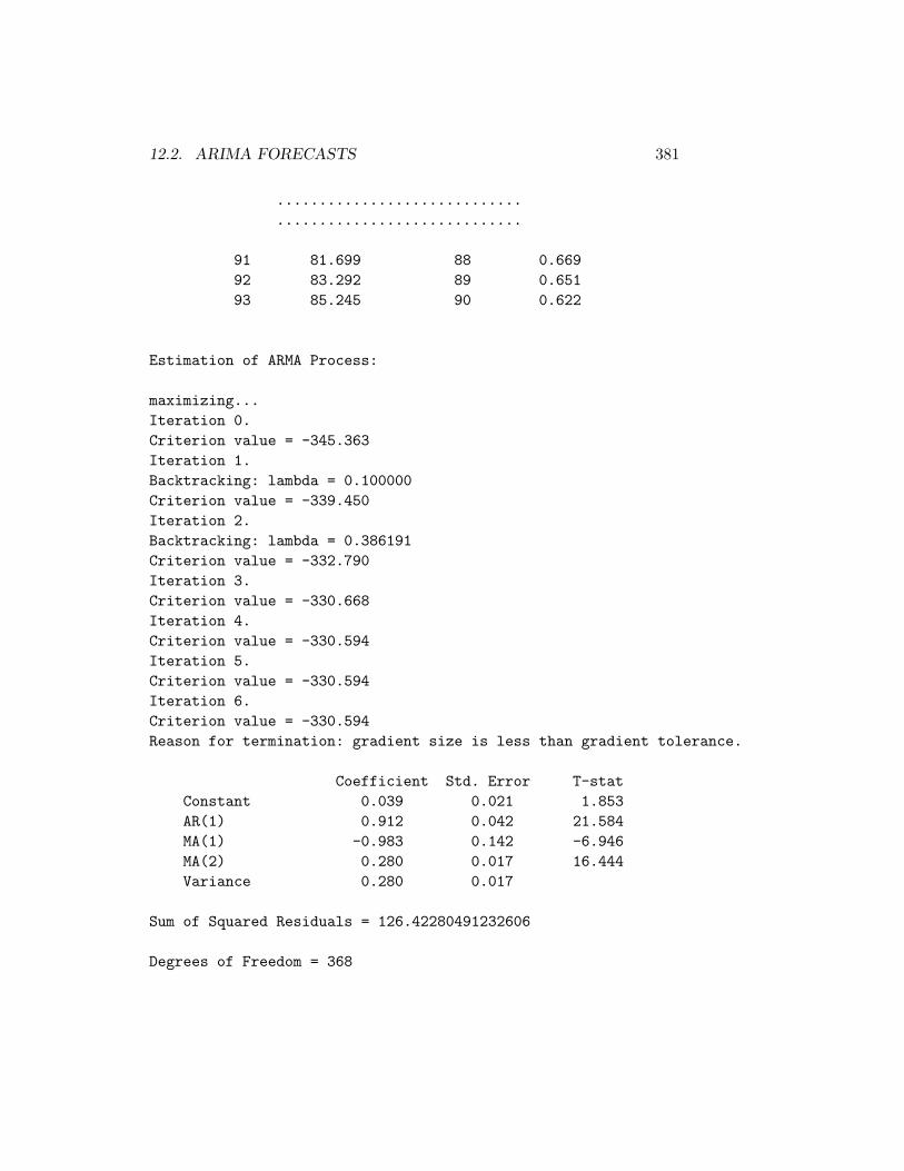
12.2. ARIMA FORECASTS 381
.............................
.............................
91 81.699 88 0.66992 83.292 89 0.65193 85.245 90 0.622
Estimation of ARMA Process:
maximizing...Iteration 0.Criterion value = -345.363Iteration 1.Backtracking: lambda = 0.100000Criterion value = -339.450Iteration 2.Backtracking: lambda = 0.386191Criterion value = -332.790Iteration 3.Criterion value = -330.668Iteration 4.Criterion value = -330.594Iteration 5.Criterion value = -330.594Iteration 6.Criterion value = -330.594Reason for termination: gradient size is less than gradient tolerance.
Coefficient Std. Error T-statConstant 0.039 0.021 1.853AR(1) 0.912 0.042 21.584MA(1) -0.983 0.142 -6.946MA(2) 0.280 0.017 16.444Variance 0.280 0.017
Sum of Squared Residuals = 126.42280491232606
Degrees of Freedom = 368

382 CHAPTER 12. FORECASTING
AIC = 1806.343060866396SBC = 1818.0997424292154
Ljung-Box Q-statistics:LAG Q DF Pval4 36.610 1 0.0005 37.240 2 0.0006 37.487 3 0.000
.............................
.............................
.............................
91 164.182 88 0.00092 166.179 89 0.00093 170.849 90 0.000
The ARMA(1,1) process clearly gives the best fit because it produces resid-uals that are not serially correlated and AIC and SBC statistics that aresmaller than the corresponding AIC and SBC statistics for the ARMA(1,2)process. These AIC and SBC statistics are also lower than those for theearlier fits of AR and MA processes. We should have also checked the fit ofan ARMA(2,2) process, but that is left as an exercise for the reader. All thecode for this section is contained in the file armach12.lsp and the importantresults, including those below, are in armach12.lou.
To forecast a variable a specific number of periods beyond the last periodfor which data are available I have written the function ARMA-forecast.It takes the following seven arguments in order—the series to be forecast,the number of autoregressive lags, the number of moving-average lags, a listof initial guesses regarding the parameter values, the integer 1 if a constantis to be included or 0 otherwise, the number of periods ahead to forecastand, finally, a zero if the newtonmax function is to be used or the integer1 if nelmeadmax is to be used. Again, the best procedure is to start withthe newtonmax function and, if that fails, use the nelmeadmax function toobtain parameter values that can be included in the guess list for final useof newtonmax. And again, a list called sizelist must be in the workspaceif nelmeadmax is used. The function returns a list of forecasted values calledpredval and leaves in the workspace, along with that list, lists called actual,fitted and resids giving the actual and fitted values and the residuals forthe data-period over which the ARMA process is fitted. The actual series

12.2. ARIMA FORECASTS 383
is simply the series used as the first argument when calling the function,shortened at its beginning by the number of autoregressive lags. Using theARMA(1,1) process fitted above, we construct a one-year ahead forecast ofthe log of U.S. M1 using the following code.
(def gueslist (list 0.023 0.948 -0.791 0.311))(ARMA-forecast (remove-first-element newy) 1 1 gueslist 1 12 0)(def dm1fut (remove-first (- (length dm1) 12) dm1))(def datesfut (remove-first (- (length datesmo) 12) datesmo))(def actual (combine actual dm1fut))(def fitted (combine fitted predval))(def dates (remove-first (- (length datesmo)(length actual)) datesmo))(def actual (undifference actual 0))(def actual (+ actual 59))(def fitted (undifference fitted 0))(def fitted (+ fitted 59))(def resids (- actual fitted))(def outmat (bind-columns dates actual fitted resids))(write-matrix-to-file outmat "armares1.mat")
The integer 59 was added to the final actual and fitted series to raise theirinitial values in 1974 from zero to the actual level in that year, taken as apercentage of the level in January 1962. We could have accomplished thesame thing by replacing the zero argument in the above undifference func-tion calls with the integer 59 or with the level of the series at 1974.0 on thedatelist, rounded to the nearest integer. My undifference function takes asits two arguments the series to be undifferenced or integrated and the initialstarting level. The actual and fitted values from the beginning of the year2000 to the end of 2005 are plotted in Figure 27. As can be clearly seen, theforecast for 2005 is no improvement over our earlier trend projection. Andduring the period 2000-2005 there are on occasion substantial differencesbetween actual and predicted.
I have also written an AR-forecast function to construct n-period aheadforecasts using autoregressive processes. This function will be demonstratedbelow in the section on OLS forecasting.
To obtain an unanticipated money shock series we need to be able tomake a series of one-period (pseudo) running-forecasts and subtract theseforecasted values from the actual values of each period. I have written thefunction ARMA-running-forecast to do this. The function takes the fol-lowing nine arguments, in order—the series being forecasted, the numberof autoregressive lags, the number of moving-average lags, the integer 1 if

384 CHAPTER 12. FORECASTING
200
205
210
215
220
225
230
2000 2001 2002 2003 2004 2005 2006
Per
cent
age
Incr
ease
Sin
ce J
anua
ry 1
962
ActualForecasted
Figure 27: Actual and predicted values of United States M1, for the years2000-2005 based on an ARIMA model fitted to the period 1974-2004.
a constant is to be included, 0 otherwise, the datelist to which the variablebeing forecasted conforms, the starting date of the running-forecast, theending date, the number of periods of data on which to base each period’sforecast, and the list providing guesses as to the initial values of the param-eters, organised in the same way as was done in the ARIMA-estimatefunction. The newtonmax function is always used. The nelmeadmax func-tion may have to be used initially in an application of ARIMA-estimateto obtain appropriate guesses as to the initial values of the parameters forthe first-period forecast. These can then be incorporated in a guess list foruse with newtonmax in ARMA-running-forecast. The code used to makea running forecast of the level of log U.S. M1 for the period 2000-2005 usingthe previous twenty years’ data for each month’s forecast is as follows.
(ARMA-setdata dm1 dates 1 1980.0 1999.917)(def sizelist (list .5 .5 .5 .5))(def gueslist (list 0.5 0.5 0.5 1))(ARMA-estimate newy 1 1 gueslist 1 0)(def gueslist (list 0.081 0.818 -0.358 0.220))(ARMA-estimate newy 1 1 gueslist 1 0)(ARMA-running-forecast dm1 1 1 1 datesmo 2000.0 2005.917 240 gueslist)(def predates (remove-first (- (length datesmo) 72) datesmo))(def actdm1 (remove-first (- (length dm1) 72) dm1))(def actm1 (undifference actdm1 0))(def actm1 (+ actm1 204))(def fitm1 (undifference predlist 0))

12.2. ARIMA FORECASTS 385
(def fitm1 (+ fitm1 204))(def fitm1 (- fitm1 (-(select fitm1 0)(select actm1 0))))(def resm1 (* 100 (/(- actm1 fitm1) fitm1)))(def meanerr (mean resm1))(def sqerr (inner-product resm1 resm1))(def msqerr (/ sqerr (length resm1)))(def rtmsqerr (sqrt msqerr))(princ "Mean Forecast Error = ")(princ meanerr)(terpri)(princ "Root Mean Square Error = ")(princ rtmsqerr)(terpri)(princ "Standard Deviation = ")(princ (standard-deviation resm1))(terpri)(terpri)(def rforcmat (bind-columns predates actm1 fitm1 resm1))(write-matrix-to-file rforcmat "armares2.mat")
The ARMA-running-forecast function calls repeatedly, for each period’sforecast, the ARMA-estimate function. After adjusting the levels of thefitted values to equal the actual in the first period, the integer 204 is addedto both the actual and fitted values to set their levels in January 2000 tothe percentage of the January 1962 level. The unanticipated money shock,resm1, is expressed as a percentage of that period’s fitted value, and its meanis calculated along with its standard deviation and the root-mean-square-forecast error. These are printed out to the screen and the resulting actual,fitted, and unanticipated log M1 shocks are written to the file armares2.mat.These results are
RUNNING ARIMA(1,1,1) FORECAST FOR 2000:1 to 20005:12
Mean Forecast Error = -0.8828606843913559Root Mean Square Error = 1.0287765908762225Standard Deviation = 0.5318524176337962
The actual and predicted values are plotted in Figure 28. The forecastsof log M1 are clearly worse than those obtained using a running 4-month-trend projection. This does not rule out, of course, the possibility thatsome alternative ARIMA process might have done better—not everythinghas been tried.
We should be able to do much better forecasting log M1 on the basis oflagged values not only of itself but of other variables that determine it. Thiscan be done with OLS forecasts.

386 CHAPTER 12. FORECASTING
200
205
210
215
220
225
230
2000 2001 2002 2003 2004 2005 2006Per
cent
age
Incr
ease
Sin
ce J
anua
ry 1
962
ACTUAL AND PREDICTED M1 AS PERCENTAGES OF 1962 LEVELS
ActualForecasted
-2
-1.5
-1
-0.5
0
0.5
1
1.5
2
2000 2001 2002 2003 2004 2005 2006
UNANTICIPATED M1 SHOCKS AS PERCENTAGES OF PREDICTED LEVELS
Figure 28: Actual and predicted values of United States M1, for the years2000-2005 in the top panel, based on running one-period ARIMA projectionsof values for twenty-four months preceeding each forecasted value.
12.3 OLS Forecasts
We begin with OLS forecasts based solely on lagged values of the series beingforecasted. This procedure uses my AR-forecast function which takes asits three arguments, in order, the series being forecasted, the number oflags, and the number of periods ahead that are to be forecasted. Afterexperimenting with autoregressive processes running from AR(1) throughAR(5), a 12-month-ahead forecast beginning in January 2005 was madeusing an AR(2) process. The batch code (which can be found along withthe code for the previous section in armach12.lsp) is as follows.

12.3. OLS FORECASTS 387
(def m1fut (remove-first (- (length m1) 12) m1))(def datesfut (remove-first (- (length datesmo) 12) datesmo))
(ARMA-setdata m1 dates 5 1974.0 2004.917);(AR-estimate (remove-first 4 newy) 1)(AR-estimate (remove-first 3 newy) 2)(AR-estimate (remove-first 2 newy) 3)(AR-estimate (remove-first 1 newy) 4)(AR-estimate newy 5);(AR-forecast (remove-first 3 newy) 2 12);(def actual (combine actual m1fut))(def fitted (combine fitted xpred))(def dates (remove-first (- (length datesmo)(length actual)) datesmo))(def outmat (bind-columns dates actual fitted))(write-matrix-to-file outmat "arres0.mat")
The results for the AR(2) case (the other results are in the file arres.lou)are as follows.
Estimation of AR Process:
Coefficient Std. Error T-Statistic P-Value
Constant 0.589 0.105 5.627 0.000AR(1) 1.293 0.050 25.986 0.000AR(2) -0.295 0.050 -5.942 0.000
Sum of Squared Residuals = 125.67741393649648
Degrees of Freedom = 369
AIC = 1804.1432511850771SBC = 1815.8999327478966
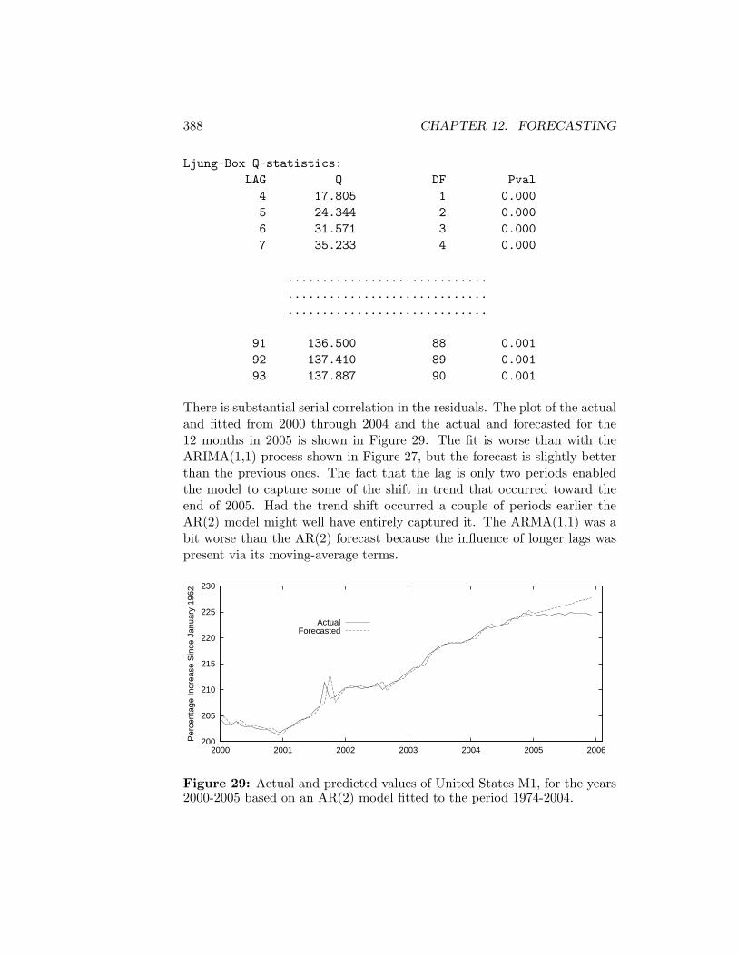
388 CHAPTER 12. FORECASTING
Ljung-Box Q-statistics:LAG Q DF Pval4 17.805 1 0.0005 24.344 2 0.0006 31.571 3 0.0007 35.233 4 0.000
.............................
.............................
.............................
91 136.500 88 0.00192 137.410 89 0.00193 137.887 90 0.001
There is substantial serial correlation in the residuals. The plot of the actualand fitted from 2000 through 2004 and the actual and forecasted for the12 months in 2005 is shown in Figure 29. The fit is worse than with theARIMA(1,1) process shown in Figure 27, but the forecast is slightly betterthan the previous ones. The fact that the lag is only two periods enabledthe model to capture some of the shift in trend that occurred toward theend of 2005. Had the trend shift occurred a couple of periods earlier theAR(2) model might well have entirely captured it. The ARMA(1,1) was abit worse than the AR(2) forecast because the influence of longer lags waspresent via its moving-average terms.
200
205
210
215
220
225
230
2000 2001 2002 2003 2004 2005 2006
Per
cent
age
Incr
ease
Sin
ce J
anua
ry 1
962
ActualForecasted
Figure 29: Actual and predicted values of United States M1, for the years2000-2005 based on an AR(2) model fitted to the period 1974-2004.

12.3. OLS FORECASTS 389
An advantage of OLS one-period-ahead forecasts is that they can bebased on lagged values of variables other than the one being forecasted. MyOLS-running-forecast function is designed to do these. It takes as itsarguments, in order—the series we want to forecast, the matrix of laggedvalues of the variables used to forecast the series (including its own pastvalues), the datelist to which these variables conform, the integer 1 if aconstant is to be included or 0 otherwise, the number of observations toinclude in the regression or, alternatively, the date in the datelist at whichall forecasting regressions are to begin (the date must contain a decimalpoint so as to not be interpreted as an integer), the starting date for the listof forecasted values, and finally, the ending date for the list of forecastedvalues. A list of forecasted values, called predlist, and a list giving theactual values for the forecast period, called actlist are left in the workspacealong with a corresponding datelist, called predates.
To illustrate we conduct an OLS-running forecast of the log of U.S. M1for the period 2000 through 20005 using data 25 years of data for eachforecast. One and three lags of the M1 variable are included along withthree lags of the logarithm of the product of the U.S. CPI and U.S. indus-trial production, to simulate a nominal GDP measure. The code for thesecalculations, which can be found in the file olsch12.lsp is as follows.
(load "addfuncs")(load "causdat")(load "maximize");(def logm1 (* 100 (log usm1sa)))(def m1 (- logm1 (select logm1 0)))(def logip (* 100 (log usindpro)))(def ip (- logip (select logip 0)))(def logcpi (* 100 (log uscpi)))(def cpi (- logcpi (select logcpi 0)))(def nip (+ ip cpi));(def usm1 (set-time-series m1 datesmo 1974.0 2005.917 0))(def m1lags (set-time-series m1 datesmo 1974.0 2005.917 3))(def m1lags (bind-columns (select laglist 1)(select laglist 3)))(def niplags (set-time-series nip datesmo 1974.0 2005.917 3))
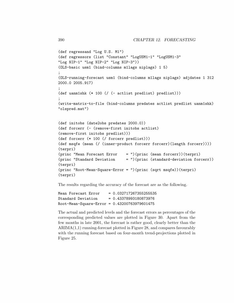
390 CHAPTER 12. FORECASTING
(def regressand "Log U.S. M1")(def regressors (list "Constant" "LogUSM1-1" "LogUSM1-3""Log NIP-1" "Log NIP-2" "Log NIP-3"))(OLS-basic usm1 (bind-columns m1lags niplags) 1 5);(OLS-running-forecast usm1 (bind-columns m1lags niplags) adjdates 1 3122000.0 2005.917);(def uanm1shk (* 100 (/ (- actlist predlist) predlist)));(write-matrix-to-file (bind-columns predates actlist predlist uanm1shk)"olspred.mat")
(def initobs (date2obs predates 2000.0))(def forcerr (- (remove-first initobs actlist)(remove-first initobs predlist)))(def forcerr (* 100 (/ forcerr predlist)))(def msqfe (mean (/ (inner-product forcerr forcerr)(length forcerr))))(terpri)(princ "Mean Forecast Error = ")(princ (mean forcerr))(terpri)(princ "Standard Deviation = ")(princ (standard-deviation forcerr))(terpri)(princ "Root-Mean-Square-Error = ")(princ (sqrt msqfe))(terpri)(terpri)
The results regarding the accuracy of the forecast are as the following.
Mean Forecast Error = 0.032717267355255535Standard Deviation = 0.43378993180873976Root-Mean-Square-Error = 0.43200763979601475
The actual and predicted levels and the forecast errors as percentages of thecorresponding predicted values are plotted in Figure 30. Apart from thefew months in late 2001, the forecast is rather good, clearly better than theARIMA(1,1) running-forecast plotted in Figure 28, and compares favourablywith the running forecast based on four-month trend-projections plotted inFigure 25.

12.4. NEAR-VAR FORECASTS 391
200
205
210
215
220
225
230
2000 2001 2002 2003 2004 2005 2006
Per
cent
age
Incr
ease
Sin
ce J
anua
ry 1
962
ActualForecasted
-2
-1.5
-1
-0.5
0
0.5
1
1.5
2
2000 2001 2002 2003 2004 2005 2006
UNANTICIPATED M1 SHOCKS AS PERCENTAGES OF PREDICTED LEVELS
Figure 30: Actual and predicted values of United States log M1, for theyears 2000-2005 in the top panel, based on running OLS one-period aheadforecasts based on one and three lags of log M1 and three lags of the log ofthe product of the U.S. consumer price index and U.S. industrial production.The forecasts are based on the preceeding twenty-five years of data.
12.4 Near-VAR Forecasts
In order to forecast ahead more than one period on the basis of currentlyavailable information using lags of variables other than the one being fore-casted, one must use a VAR in all variables—their predicted levels in eachperiod are added to that period’s data and new predicted levels are calcu-lated. Repeated calculations of this sort yield forecasts for as many periodsahead that one might choose. The problem is, however, that insignificantlagged variables in the VAR equations create excess random variability ofthe predicted results. A more appropriate procedure, therefore, is to use a

392 CHAPTER 12. FORECASTING
Near-VAR—that is a VAR in which insignificant lags of variables are omit-ted. This requires that seemingly-unrelated-regression techniques be usedinstead of OLS to obtain efficient coefficient estimates and, hence, forecastedvalues. To illustrate, we modify the basic U.S. VAR that we used in Chap-ter 10, involving the log real GDP, the log of the implicit GDP deflator, the1-month commercial paper rate and the log of M1. The estimation periodthere ran from 1965 through 2005. Here we will estimate for the period 1965through 2004 and forecast the values for the year 2005. Since the data arequarterly, this will involve forecasting one through four periods ahead.
First we must set up the data and determine which lags in the VARequations are statistically significant. Because this is an illustration and notan attempt at actual economic analysis, we will simply pick out the lags thatwere significant in the original VAR, re-estimate the four equations by OLSand then routinely drop any lags that are insignificant on re-estimation.It is important to note here that we require only that the model predictefficiently, not that it necessarily reflect channels of causation. The finalregression results for the period 1965 through 2004 are as follows (the batchcode from which these results were produced will be shown later).
LINEAR REGRESSION
Dependent Variable: Log Real GDP
Coefficient Std. Error T-stat P-Val
Constant 0.186 0.055 3.399 0.001LogRGDP-L1 0.972 0.010 100.977 0.000Intrate-L2 -0.258 0.056 -4.640 0.000Intrate-L3 0.138 0.056 2.469 0.015LogM1-L3 0.011 0.005 2.377 0.019
Number of Observations: 160Degrees of Freedom: 155R-Squared: 0.999557455376693Adjusted R-Squared: 0.9995460348702851Sum of Squared Errors: 0.008789311293886626LMSC -- Chi-Square: 5.829305158209041P-Value: 0.0157613476752545Breusch-Pagan -- Chi-Square: 9.326330323771614P-Value: 0.05344072356438134Regression F-Statistic: 87523.04141989283P-Value: 0.0

12.4. NEAR-VAR FORECASTS 393
LINEAR REGRESSION
Dependent Variable: Log Implicit GDP Deflator
Coefficient Std. Error T-stat P-Val
Constant 0.006 0.002 2.590 0.011LogPlev-L1 1.568 0.077 20.291 0.000LogPlev-L2 -0.417 0.112 -3.712 0.000LogPlev-L4 -0.153 0.039 -3.901 0.000
Number of Observations: 160Degrees of Freedom: 156R-Squared: 0.9999707950999939Adjusted R-Squared: 0.9999702334673015Sum of Squared Errors: 0.0012320831106580948LMSC -- Chi-Square: 1.0738481497725598P-Value: 0.3000778548158437
Breusch-Pagan -- Chi-Square: 25.034837433874806P-Value: 1.5183684072717085E-5
Regression F-Statistic: 1780471.131021227P-Value: 0.0
LINEAR REGRESSION
Dependent Variable: Interest Rate
Coefficient Std. Error T-stat P-Val
Constant 0.017 0.021 0.797 0.427LogRGDP-L1 0.225 0.068 3.307 0.001LogRGDP-L3 -0.227 0.068 -3.360 0.001Intrate-L1 1.120 0.076 14.723 0.000Intrate-L2 -0.506 0.110 -4.614 0.000Intrate-L3 0.651 0.113 5.772 0.000Intrate-L4 -0.308 0.074 -4.152 0.000

394 CHAPTER 12. FORECASTING
Number of Observations: 160Degrees of Freedom: 153R-Squared: 0.9065564884000686Adjusted R-Squared: 0.9028920369647773Sum of Squared Errors: 0.014366766923784245LMSC -- Chi-Square: 0.6341008864671108P-Value: 0.42585505980579075Breusch-Pagan -- Chi-Square: 36.03414748415517P-Value: 2.714819091087506E-6Regression F-Statistic: 247.3921416093136P-Value: 0.0
LINEAR REGRESSION
Dependent Variable: Log M1
Coefficient Std. Error T-stat P-Val
Constant 0.013 0.007 1.978 0.050Intrate-L1 -0.398 0.058 -6.915 0.000Intrate-L2 0.508 0.088 5.790 0.000Intrate-L3 -0.105 0.061 -1.709 0.089LogM1-L1 1.684 0.057 29.284 0.000LogM1-L2 -0.685 0.057 -11.954 0.000
Number of Observations: 160Degrees of Freedom: 154R-Squared: 0.9998803132804434Adjusted R-Squared: 0.9998764273479902Sum of Squared Errors: 0.009087992417913001LMSC -- Chi-Square: 6.865609076962485P-Value: 0.008787029300850069Breusch-Pagan -- Chi-Square: 12.84909623887291P-Value: 0.024834693104760386Regression F-Statistic: 257307.69264219378P-Value: 0.0

12.4. NEAR-VAR FORECASTS 395
The estimation of Near-VAR’s is a bit tricky so the code used will berather carefully exposited. First, we set up our data to run from 1965through 2005. The batch file containing all the code illustrated below isnvarch12.lsp and the results from processing this code are in nvarch12.lou.
(def uscpapr (m2q-avg uscpapr 0 1962.0 2005.75))(def usm1 (m2q-avg usm1sa 0 1962.0 2005.75));(def usipd (remove-first 16 usipd)) ; remove observations(def usrgdp (remove-first 16 usrgdp)) ; for 1959, 1960, 1961(def datesq (remove-first 16 datesq)) ; and 1962;(def logrgdp (log usrgdp)) ; take logarithms(def logipd (log usipd))(def logm1 (remove-first 4 (log usm1))) ; remove 1962 observation(def intrate (/ (remove-first 4 (copy-list uscpapr)) 100))
; convert interest rate from % to fraction
We then set aside the actual levels of the variables for the period 2000-2005which we will later plot along with our predicted values. After doing this,we eliminate the 2005 observations from the series that will be used in initialestimation and from the datelist that will be used.
(def actrgdp (remove-first (- (length logrgdp) 24)(copy-list logrgdp)))(def rgdp (copy-list (remove-last 4 logrgdp)))(def actplev (remove-first (- (length logipd) 24)(copy-list logipd)))(def plev (copy-list (remove-last 4 logipd)))(def actintr (remove-first (- (length intrate) 24)(copy-list intrate)))(def intr (copy-list (remove-last 4 intrate)))(def actmon1 (remove-first (- (length logm1) 24)(copy-list logm1)))(def mon1 (copy-list (remove-last 4 logm1)))(def dates (copy-list (remove-last 4 dates)))
Each time we set up the data for estimation using the set-time-series func-tion, the first eight observations of the current values of the four variableswe are using will be lopped off. We need to set these aside so that they canbe added after each of the four passes we will need to forecast four periodsahead. Then we can begin our dotimes loop.
(def begrgdp (remove-last (- (length logrgdp) 8) logrgdp))(def begplev (remove-last (- (length logipd) 8) logipd))(def begintr (remove-last (- (length intrate) 8) intrate))

396 CHAPTER 12. FORECASTING
(def begmon1 (remove-last (- (length logm1) 8) logm1));(dotimes (i 4)
After setting the code to print the run number at the beginning of eachrun, we instruct the interpreter to prepare four lagged values of each of thevariables along with its current value. Recall that the laglist object leftin the workspace by the set-time-series function gives a list of the currentand four lagged values of the series. We set the fourth argument in theset-time-series function to augment the ending date of estimation by onequarter after each run. Recall also that the four values of i will be 0, 1, 2and 3.
(terpri)(princ "RUN NUMBER= ")(princ i)(terpri)(terpri)(def rgdplags (set-time-series rgdp dates 1965.0 (+ 2004.75 (* .25 i)) 4))(def rgdp (select laglist 0))(def rgdp-1 (select laglist 1))(def rgdp-2 (select laglist 2))(def rgdp-3 (select laglist 3))(def rgdp-4 (select laglist 4))(def ipdlags (set-time-series plev dates 1965.0 (+ 2004.75 (* .25 i)) 4))(def plev (select laglist 0))(def plev-1 (select laglist 1))(def plev-2 (select laglist 2))(def plev-3 (select laglist 3))(def plev-4 (select laglist 4))(def intlags (set-time-series intr dates 1965.0 (+ 2004.75 (* .25 i)) 4))(def intr (select laglist 0))(def intr-1 (select laglist 1))(def intr-2 (select laglist 2))(def intr-3 (select laglist 3))(def intr-4 (select laglist 4))(def m1lags (set-time-series mon1 dates 1965.0 (+ 2004.75 (* .25 i)) 4))(def mon1 (select laglist 0))(def mon1-1 (select laglist 1))(def mon1-2 (select laglist 2))(def mon1-3 (select laglist 3))(def mon1-4 (select laglist 4))
We then run the four regressions and extract the residuals.
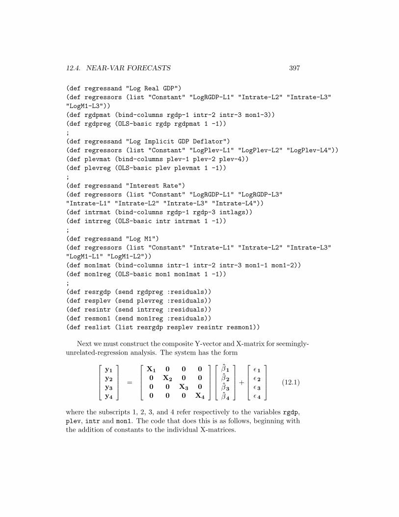
12.4. NEAR-VAR FORECASTS 397
(def regressand "Log Real GDP")(def regressors (list "Constant" "LogRGDP-L1" "Intrate-L2" "Intrate-L3""LogM1-L3"))(def rgdpmat (bind-columns rgdp-1 intr-2 intr-3 mon1-3))(def rgdpreg (OLS-basic rgdp rgdpmat 1 -1));(def regressand "Log Implicit GDP Deflator")(def regressors (list "Constant" "LogPlev-L1" "LogPlev-L2" "LogPlev-L4"))(def plevmat (bind-columns plev-1 plev-2 plev-4))(def plevreg (OLS-basic plev plevmat 1 -1));(def regressand "Interest Rate")(def regressors (list "Constant" "LogRGDP-L1" "LogRGDP-L3""Intrate-L1" "Intrate-L2" "Intrate-L3" "Intrate-L4"))(def intrmat (bind-columns rgdp-1 rgdp-3 intlags))(def intrreg (OLS-basic intr intrmat 1 -1));(def regressand "Log M1")(def regressors (list "Constant" "Intrate-L1" "Intrate-L2" "Intrate-L3""LogM1-L1" "LogM1-L2"))(def mon1mat (bind-columns intr-1 intr-2 intr-3 mon1-1 mon1-2))(def mon1reg (OLS-basic mon1 mon1mat 1 -1));(def resrgdp (send rgdpreg :residuals))(def resplev (send plevreg :residuals))(def resintr (send intrreg :residuals))(def resmon1 (send mon1reg :residuals))(def reslist (list resrgdp resplev resintr resmon1))
Next we must construct the composite Y-vector and X-matrix for seemingly-unrelated-regression analysis. The system has the form
y1
y2
y3
y4
=
X1 0 0 00 X2 0 00 0 X3 00 0 0 X4
β1
β2
β3
β4
+
ε1
ε2
ε3
ε4
(12.1)
where the subscripts 1, 2, 3, and 4 refer respectively to the variables rgdp,plev, intr and mon1. The code that does this is as follows, beginning withthe addition of constants to the individual X-matrices.

398 CHAPTER 12. FORECASTING
(def consterm (repeat 1 nobs))(def rgdpmat (bind-columns consterm rgdpmat))(def plevmat (bind-columns consterm plevmat))(def intrmat (bind-columns consterm intrmat))(def mon1mat (bind-columns consterm mon1mat));(def zeromat (make-array (array-dimensions rgdpmat) :initial-element 0))(def rgdpseg (bind-rows rgdpmat zeromat zeromat zeromat))(def zeromat (make-array (array-dimensions plevmat) :initial-element 0))(def plevseg (bind-rows zeromat plevmat zeromat zeromat))(def zeromat (make-array (array-dimensions intrmat) :initial-element 0))(def intrseg (bind-rows zeromat zeromat intrmat zeromat))(def zeromat (make-array (array-dimensions mon1mat) :initial-element 0))(def mon1seg (bind-rows zeromat zeromat zeromat mon1mat))(def SURXmat (bind-columns rgdpseg plevseg intrseg mon1seg));(def SURYvar (append rgdp plev intr mon1))
Then we have to create the matrix of system residuals, which takes thefollowing form.
Ω =
s 21 I s12 I s13 I s14 I
s12 I s 22 I s23 I s24 I
s13 I s23 I s 23 I s34 I
s14 I s24 I s34 I s 24 I
This is done as follows.
(def rgdprgdp (/ (inner-product resrgdp resrgdp) nobs))(def rgdpplev (/ (inner-product resrgdp resplev) nobs))(def rgdpintr (/ (inner-product resrgdp resintr) nobs))(def rgdpmon1 (/ (inner-product resrgdp resmon1) nobs));(def plevrgdp (/ (inner-product resplev resrgdp) nobs))(def plevplev (/ (inner-product resplev resplev) nobs))(def plevintr (/ (inner-product resplev resintr) nobs))(def plevmon1 (/ (inner-product resplev resmon1) nobs));(def intrrgdp (/ (inner-product resintr resrgdp) nobs))(def intrplev (/ (inner-product resintr resplev) nobs))(def intrintr (/ (inner-product resintr resintr) nobs))(def intrmon1 (/ (inner-product resintr resmon1) nobs))
12.4. NEAR-VAR FORECASTS 399
;(def mon1rgdp (/ (inner-product resmon1 resrgdp) nobs))(def mon1plev (/ (inner-product resmon1 resplev) nobs))(def mon1intr (/ (inner-product resmon1 resintr) nobs))(def mon1mon1 (/ (inner-product resmon1 resmon1) nobs));(def identmat (identity-matrix nobs));(def rgdpseg(bind-rows (* rgdprgdp identmat)(* rgdpplev identmat)(* rgdpintr identmat)(* rgdpmon1 identmat)))(def plevseg(bind-rows (* plevrgdp identmat)(* plevplev identmat)(* plevintr identmat)(* plevmon1 identmat)))(def intrseg(bind-rows (* intrrgdp identmat)(* intrplev identmat)(* intrintr identmat)(* intrmon1 identmat)))(def mon1seg(bind-rows (* mon1rgdp identmat)(* mon1plev identmat)(* mon1intr identmat)(* mon1mon1 identmat)));(def SURomega (bind-columns rgdpseg plevseg intrseg mon1seg))
We are now ready to estimate the system using GLS.
(def regressand "SUR: RGDP PLEV INTR MON1")(def regressors (list "Constant" "RGDP-L1" "INTR-L2" "INTR-L3" "MON1-L3""Constant" "PLEV-L1" "PLEV-L2" "PLEV-L4""Constant" "RGDP-L1" "RGDP-L3" "INTR-L1" "INTR-L2" "INTR-L3" "INTR-L4""Constant" "Intrate-L1" "Intrate-L2" "Intrate-L3" "LogM1-L1" "LogM1-L2"))(GLS SURYvar SURXmat SURomega)
Next we extract from GLScoefs, the list of coefficients left in the workspaceby the GLS function, the coefficients that relate to each of the four variables.
(def rgdpcoef (remove-last 17 GLScoefs)) ; leaves 5 rgdp coefs(def plevcoef (remove-first 5 GLScoefs)) ; removes 5 rgdp coefs(def plevcoef (remove-last 13 plevcoef)) ; removes intr and mon1 coefs(def intrcoef (remove-last 6 GLScoefs)) ; removes mon1 coefs(def intrcoef (remove-first 9 intrcoef)) ; removes rgdp and plev coefs(def mon1coef (remove-first 16 GLScoefs)) ; removes all but mon1 coefs

400 CHAPTER 12. FORECASTING
Then we construct lists of the relevant lagged values of the four variables thatdetermine the current value of each variable in turn, and then multiply theseby the relevant coefficients to obtain the predicted values of each variablefor the first quarter of 2005 and add it to the list of observations for thatvariable.
(def rgdplist (list 1.0(select rgdp (- (length rgdp) 1))(select intr (- (length intr) 2))(select intr (- (length intr) 3))(select mon1 (- (length mon1) 3))))(def rgdppred (inner-product rgdpcoef rgdplist))(def rgdp (append rgdp (list rgdppred)));(def plevlist (list 1.0(select plev (- (length plev) 1))(select plev (- (length plev) 2))(select plev (- (length plev) 4))))(def plevpred (inner-product plevcoef plevlist))(def plev (append plev (list plevpred)));(def intrlist (list 1.0(select rgdp (- (length rgdp) 1))(select rgdp (- (length rgdp) 3))(select intr (- (length intr) 1))(select intr (- (length intr) 2))(select intr (- (length intr) 3))(select intr (- (length intr) 4))))(def intrpred (inner-product intrcoef intrlist))(def intr (append intr (list intrpred)));(def mon1list (list 1.0(select intr (- (length intr) 1))(select intr (- (length intr) 2))(select intr (- (length intr) 3))(select mon1 (- (length mon1) 1))(select mon1 (- (length mon1) 2))))(def mon1pred (inner-product mon1coef mon1list))(def mon1 (append mon1 (list mon1pred)))
In order to check our results we print out the predicted level of each variable
12.4. NEAR-VAR FORECASTS 401
and then the last five values of the new list of observations for that variableto make sure that the last observation on the list is in fact the predictedvalue.
(terpri)(princ "Predicted RGDP = ")(princ rgdppred)(terpri)(princ "Last five RGDP = ")(terpri)(princ (last-five rgdp))(terpri);(terpri)(princ "Predicted PLEV = ")(princ plevpred)(terpri)(princ "Last five PLEV = ")(terpri)(princ (last-five plev))(terpri);(terpri)(princ "Predicted INTR = ")(princ intrpred)(terpri)(princ "Last five INTR = ")(terpri)(princ (last-five intr))(terpri);(terpri)(princ "Predicted MON1 = ")(princ mon1pred)(terpri)(princ "Last five MON1 = ")(terpri)(princ (last-five mon1))(terpri)
Finally, we add the first-quarter of 2005 to the datelist to be used as anargument in the set-time-series function in the next round and add thepre-1965 values back onto the lists representing the respective variables tobe used in establishing the relevant lags for estimating their 1965 levels.That then brings us to the end of our dotimes loop.
(def dates (append dates (list (+ (select dates (- (length dates) 1)) .25))))(def rgdp (append begrgdp rgdp))(def plev (append begplev plev))(def intr (append begintr intr))(def mon1 (append begmon1 mon1))) ; end dotimes i
The interpreter will now run through the loop three more times, calcu-lating the predicted values for the second, third and fourth quarters of 2005and adding them to the ends of the series for each variable.
The last step is to plot the results in XLispStat and write them to fileso that we can plot them using Gnuplot. We first remove all pre-2000observations from the actual levels of our variables saved above and fromthe series to which the predicted levels were added, and we then adjust bothto express all observations as percentages of their levels in the first quarterof 2000.

402 CHAPTER 12. FORECASTING
(def predrgdp (remove-first (- (length rgdp) 24) rgdp))(def predplev (remove-first (- (length plev) 24) plev))(def predintr (remove-first (- (length intr) 24) intr))(def predmon1 (remove-first (- (length mon1) 24) mon1))(def plotdates (remove-first (- (length datesq) 24) datesq));(def actrgdp (* 100 actrgdp))(def actrgdp (+ 100 (- actrgdp (select actrgdp 0))))(def predrgdp (* 100 predrgdp))(def predrgdp (+ 100 (- predrgdp (select predrgdp 0))))(def actplev (* 100 actplev))(def actplev (+ 100 (- actplev (select actplev 0))))(def predplev (* 100 predplev))(def predplev (+ 100 (- predplev (select predplev 0))))(def actmon1 (* 100 actmon1))(def actmon1 (+ 100 (- actmon1 (select actmon1 0))))(def predmon1 (* 100 predmon1))(def predmon1 (+ 100 (- predmon1 (select predmon1 0))))(def actintr (* 100 actintr))(def predintr (* 100 predintr));(write-matrix-to-file (bind-columns plotdates actrgdp predrgdpactplev predplev actintr predintr actmon1 predmon1) "stmlspf31.mat");(def plot1 (plot-lines (- plotdates 1900) actrgdp :title "RGDP"))(send plot1 :add-points (- plotdates 1900) actrgdp)(send plot1 :add-lines (- plotdates 1900) predrgdp)(def plot2 (plot-lines (- plotdates 1900) actplev :title "PLEV"))(send plot2 :add-points (- plotdates 1900) actplev)(send plot2 :add-lines (- plotdates 1900) predplev)(def plot3 (plot-lines (- plotdates 1900) actintr :title "INTR"))(send plot3 :add-points (- plotdates 1900) actintr)(send plot3 :add-lines (- plotdates 1900) predintr)(def plot4 (plot-lines (- plotdates 1900) actmon1 :title "MON1"))(send plot4 :add-points (- plotdates 1900) actmon1)(send plot4 :add-lines (- plotdates 1900) predmon1)
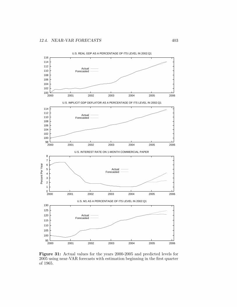
12.4. NEAR-VAR FORECASTS 403
100
102
104
106
108
110
112
114
116
2000 2001 2002 2003 2004 2005 2006
U.S. REAL GDP AS A PERCENTAGE OF ITS LEVEL IN 2002:Q1
ActualForecasted
98
100
102
104
106
108
110
112
114
2000 2001 2002 2003 2004 2005 2006
U.S. IMPLICIT GDP DEFLATOR AS A PERCENTAGE OF ITS LEVEL IN 2002:Q1
ActualForecasted
0
1
2
3
4
5
6
7
8
2000 2001 2002 2003 2004 2005 2006
Per
cent
Per
Yea
r
U.S. INTEREST RATE ON 1-MONTH COMMERCIAL PAPER
ActualForecasted
95
100
105
110
115
120
125
130
2000 2001 2002 2003 2004 2005 2006
U.S. M1 AS A PERCENTAGE OF ITS LEVEL IN 2002:Q1
ActualForecasted
Figure 31: Actual values for the years 2000-2005 and predicted levels for2005 using near-VAR forecasts with estimation beginning in the first quarterof 1965.
404 CHAPTER 12. FORECASTING
The resulting forecasts for the year 2005, together with the actual valuesare presented in Figure 31. The forecasts of real GDP and the price levelare quite good but, as with all previous forecasts, the trend-shift in M1 wasmissed. And a shift in trend that did not in fact occur was forecasted in thecase of the interest rate on commercial paper.
12.4. NEAR-VAR FORECASTS 405
References
Bernanke, Ben (1986), “Alternative Explanations of Money-Income Corre-lation,” Carnegie-Rochester Conference Series on Public Policy 25, 49–100.
Blanchard, Olivier Jean and Danny Quah (1989), “The Dynamic Effects ofAggregate Demand and Supply Disturbances,” American Economic Review,Vol. 79, 655-673.
Breusch, T. S. (1978), “Testing for Autocorrelation in Dynamic LinearModels,” Australian Economic Papers, Vol. 17, 334-355.
Breusch, T. S. and A. R. Pagan (1979), “A Simple Test for Heteroskedastic-ity and Random Coefficient Variation,” Econometrica, Vol. 47, 1287-1294.
Carr, Jack (1972), “A Suggestion for the Treatment of Serial Correlation:A Case in Point,” Canadian Journal of Economics, Vol. 2, 301-306.
Carr, Jack and Michael Darby (1981), “The Role of Money Supply Shocksin the Short-run Demand for Money,” 183-199.
Chiang, Alpha C. (1984) Fundamental Methods of Mathematical Economics,Third Edition, McGraw-Hill.
Christiano, Lawrence J., Martin Eichenbaum and Charles L. Evans (1999),“Monetary Policy Shocks: What Have We Learned and to What End?”, inJohn B. Taylor and Michael Woodford, eds., Handbook of Macroeconomics,Volume 1A, Elsevier Press, Chapter 2, 65-148.
Cochrane, D. and Guy H. Orcutt (1949), “Application of Least-Squares Re-gression to Relationships Containing Auto-correlated Error Terms,” Journalof the American Statistical Association, Vol. 44, 32-61.
Dickey, David A. and Wayne A. Fuller (1981), “Likelihood Ratio Statisticsfor Autoregressive time Series with a Unit Root,” Econometrica, Vol. 49,P. 1063.
Enders, Walter (1995), Applied Econometric Time Series, Wiley Series inProbability and Mathematical Statistics, John Wiley & Sons.
Engle, Robert F. and C. W. J. Granger (1983), “Co-Integration and Er-ror Correction: Representation, Estimation, and Testing,” Econometrica,Vol. 55, 251-276.

406 CHAPTER 12. FORECASTING
Engle, Robert F. and Byung Sam Yoo (1987), “Forecasting and Testing inCo-Integrated Systems,” Journal of Econometrics, Vol. 35, 143-159.
Fuller, Wayne A. (1976), Introduction to Statistical Time Series, Wiley.
Godfrey, L. G. (1978), “Testing for Higher Order Serial Correlation inRegression Equations When the Regressors Include Lagged DependentVariables,” Econometrica, Vol. 46, 1303-1310.
Hamilton, James D. (1994), Time Series Analysis, Princeton UniversityPress.
Hildreth, Clifford and John Y. Lu (1960), Demand Relations with Autocorre-lated Disturbances, Agriculture Experiment Station Technical Bulletin 276,Michigan State University, East-Lansing, Michigan.
Johansen, Soren (1988), “Statistical Analysis of Cointegration Vectors,”Journal of Economic Dynamics and Control, Vol. 12, 221-254.
Johnston, Jack and John DiNardo (1997), Econometric Methods, McGraw-Hill.
Maddala, G. S. (1988), Introduction to Econometrics, Macmillan.
McFadden, D. (1974), “The Measurement of Urban Travel Demand,”Journal of Political Economy, Vol. 93, 417-425.
Munnell, Alicia H. and Geoffrey M. B. Tootell, Lynne E. Browne and JamesMcEneaney (1996), “Mortgage Lending in Boston: Interpreting the HMDAData,” American Economic Review, Vol. 66, 25-53.
Newey, Whitney and Kenneth West (1987), “A Simple Positive Semi-Definite,Heteroskedastic and Autocorrelation Consistent Covariance Matrix,”Econometrica, Vol. 55, 703-708.
Phillips, P. C. B. (1987), “Understanding Spurious Regression inEconometrics,” Journal of Econometrics, Vol. 33, 311-340.
Phillips, P. C. B. and Pierre Perron (1988), “Testing for a Unit Root inTime Series Regression,” Econometrica, Vol. 75, 335-346.
Phillips, P. C. B. and S. Ouliaris (1990), “Asymptotic Properties of ResidualBased Tests for Cointegration,” Econometrica, Vol. 58, 189-190.
Said, S. and David A. Dickey (1984), “Testing for Unit Roots in Autoregressive-Moving-Average Models of Unknown Order,”Biometrika,Vol. 71, 599-607.

12.4. NEAR-VAR FORECASTS 407
Sims, Christopher (1986), “Are Forecasting Models Usable for Policy Analy-sis?” Federal Reserve Bank of Minneapolis Quarterly Review, Winter, 3–16.
Stock, James H. and Mark W. Watson (2003), Introduction to Econometrics,Addison-Wesley.
Tierney, Luke (1990), LISP-STAT: An Object-Oriented Environment forStatistical Computing, Wiley Series in Probability and Mathematical Statis-tics, John Wiley & Sons.
White, Halbert (1980), “A Heteroskedasticity-Consistent Covariance MatrixEstimator and a Direct Test for Heteroskedasticity,” Econometrica, Vol. 48,827-838.

Index
*, 6+, 6-, 6/, 6:add-lines, 55, 78:add-points, 55, 78:coef-estimates, 92:fit-values, 147:help, 91:help :coef-estimates, 92:intercept nil, 91:plot-residuals, 93:print nil, 91:residuals, 252:variable-label, 55
abs, 7, 9acf, 59, 61, 187, 375aicsbc, 183append, 11, 267, 401AR-estimate, 375AR-forecast, 383, 386AR-set-data, 375aref, 19, 29, 259ARMA-estimate, 379, 384ARMA-forecast, 382ARMA-residuals, 379ARMA-running-forecast, 383–385ARMA-set-data, 374array-dimensions, 22, 29, 43, 88
base, 39, 96
bin-sort, 82bind-columns, 19, 35, 47, 87, 118,
267, 399bind-rows, 19, 267, 399binomial-cdf, 65block-lag, 42block-lead, 42boxplot, 52bq-exch-rate-history, 341Breusch-Pagan, 95, 114
Chi-Square tests, 83chisq-cdf, 67chisq-dens, 83chisq-quant, 66chisq-rand, 72chosen-five, 17, 80close, 31coerce, 21, 87combine, 12copy-list, 13copy-matrix-column, 22, 37copy-matrix-row, 22correlation, 52, 79covariance, 52, 267CPE-test, 243create-ARMA-series, 374
date2obs, 41, 55, 97def, 8, 52, 91detrend, 41dfunit, 183, 187, 193, 195
408
INDEX 409
diagonal, 20, 334difference, 41, 56, 339dotimes, 13, 29, 35, 37, 89, 395dribble, 5Durbin-Watson, 112
error, 17exp, 7, 9exponential, 67
f-cdf, 66f-quant, 66f-rand, 72F-restriction, 105, 106find-NA-in-matrix, 35first-five, 16, 17, 39–41, 43, 44, 51format, 29, 30
GLS, 259, 264, 267, 399GLS-joint-hypothesis-test, 269
HAC-stderrs, 108help, 17histogram, 52
identity-matrix, 21, 259, 267if, 14, 131inner-product, 25, 87, 398interquartile-range, 50inverse, 25iseq, 13–15, 17, 30, 71
Johansen-coint, 205, 209Johansen-cointvector-test, 214joint-hypothesis-test, 221, 227
kernel density, 53kernel-dens, 53, 68, 71
last-five, 17, 39–41, 43, 44, 51LBQ, 102length, 11, 35, 37, 40, 43, 131
LMSC-test, 100, 106, 112, 117load, 16, 26, 28, 35log, 7, 9logit, 173, 178LogProb-LRtest, 178
m2a-avg, 40m2q-avg, 40, 47, 102, 276MA-estimate, 376, 377MA-residuals, 377make-array, 19, 23, 267matmult, 24, 87max, 10, 50mean, 49, 73, 76, 363median, 49, 50min, 10, 50multicollinearity, 106
nelmeadmax, 169, 325, 329, 354, 355,377, 380
newtonmax, 169, 173, 325, 328, 329,354, 355, 377, 380
NLLS, 165nllsreg, 164normal-cdf, 63normal-quant, 64, 80normal-rand, 72nreg-model, 163
OLS-basic, 108, 112, 117, 142, 144,155, 159, 240, 246, 252, 265,278
OLS-cross-section, 113, 114, 120, 138OLS-panel, 127OLS-running-forecast, 389OLS-time-series, 113, 115, 117, 118,
219OLS-trend-projection, 362open, 31outer-product, 25, 87

410 INDEX
pacf, 59, 61, 187, 375panel-collect-obsnums, 122panel-entity-demean, 125panel-set-fixed-effects, 126panel-switch-stack-order, 137, 139plot-binomial, 69plot-chisq, 70plot-F, 70plot-lines, 42, 53, 54, 78, 99plot-normal-on-t, 70plot-points, 54, 55plot-poisson, 70plot-standard-normal, 70plot-t, 70plot-t-on-normal, 70poisson-cdf, 66ppunit, 187, 193, 195, 228, 248, 254,
365, 372princ, 28print-matrix, 19, 23, 29, 89, 288, 315print-time-series, 115print-time-series-regression, 117probit, 170, 178prod, 10
q2a-avg, 40, 102quantile, 50
range, 50read-data-columns, 27, 32, 39read-data-file, 46, 73, 80regression-model, 90, 117remove-first, 18, 44, 46, 97, 276, 339remove-first-columns, 22remove-first-element, 18remove-first-rows, 22remove-last, 18, 44remove-last-columns, 22remove-last-element, 18remove-last-rows, 22
remove-selected element, 18remove-selected-column, 22remove-selected-row, 22, 37repeat, 12, 13, 87reverse, 12, 37running-trend-projection, 363
sample, 71savevar, 27, 34, 35, 37, 38seasdums-M, 45, 98seasdums-Q, 45, 98select, 11, 15, 27, 29, 35, 37, 43, 68,
88, 89, 122, 131, 137set-time-series, 43, 44, 118, 339, 389,
395setdates, 39, 40, 55setf, 12, 31, 89sort-data, 51sqrt, 7, 73standard-deviation, 49, 50, 73, 363stats, 50, 124sum, 10
t-cdf, 64t-quant, 64t-rand, 72terpri, 28, 31transpose, 25, 87, 259TSLS-OIR, 149, 152TSLS-panel, 148TSLS-SS-basic, 148TSLS-SS-cross-section, 148, 156TSLS-SS-time-series, 149TSLS-time-series, 148
undef, 14undifference, 383uniform-rand, 71
VAR-add-results-vectors, 343VAR-BlanQuah-decomp, 340, 341
INDEX 411
VAR-blanquah-history, 341, 358VAR-block-lag-significance, 278, 285VAR-bootstrap-values, 343VAR-calc-conf-limits, 344VAR-calc-Gmat-just-identified, 312, 314,
315, 355VAR-calc-thetlist, 327, 328VAR-check-struct-decomp, 315VAR-Choleski-decomp, 292, 294VAR-estimate-blanquah, 356, 358VAR-estimate-choleski, 344, 346, 347,
349VAR-estimate-structural, 354VAR-extend-struct-decomp, 317, 334VAR-lag-length, 204, 211, 248, 274,
276, 339VAR-MA-representation, 287, 288, 292,
314, 325, 334, 340VAR-maxlike-calc-Gmat, 327–329, 332VAR-plot-impulse-responses-of, 294,
340VAR-plot-impulse-responses-to, 294,
340VAR-print-forecast-error-variance-decompositions,
294, 340VAR-print-impulse-responses, 294, 340VAR-results-vectors, 343VAR-run-standard-form, 277, 278, 334VAR-setup, 277, 278, 285, 287, 314,
334, 340VAR-standard-form, 343VAR-write-fev-decomps-to-LaTeX-file,
294, 302variables, 8, 27, 46variance, 49, 75, 267varstd, 325, 327, 331, 355vector, 21
write-graphs-to-TeXfile, 346, 347, 349write-matrix, 29–31, 288, 315
write-matrix-to-file, 31, 389, 404

Statistical Tables
While the simplest way to calculate P-Values is to use the XLispStat cu-mulative density functions, the test-statistics for unit root and cointegrationtests do not follow standard distributions. Accordingly, the next three pagescontain the relevant statistical tables for Dickey-Fuller and Phillips-Perronunit root tests, for cointegration tests based on unit root tests of regressionresiduals, and for Johansen cointegration tests.
The critical values for the unit root tests in the table that follows werecalculated using Monte Carlo methods by David Dickey and Wayne A. Fullerand were obtained from their paper “Likelihood Ratio Statistics for Autore-gressive Time Series with a Unit Root,” Econometrica, Vol. 49, July 1981,pages 1062 and 1063, and from Walter Enders, Applied Econometric TimeSeries, Wiley Series in Probability and Mathematical Statistics, John Wi-ley & Sons, 1995, pages 223, 419 and 421, and from James D. Hamilton,Time Series Analysis, Princeton University Press, 1994, page 763. Thesecritical values are based on sample sizes of 100 and remain unchanged whenthe Dickey-Fuller estimating equations are augmented by inclusion of laggedvalues of ∆yt to improve the fit as indicated by the AIC and SBC. Largersample sizes will result in critical values that are slightly smaller in absolutevalue and smaller sample sizes will result in somewhat larger critical values.

STATISTICAL TABLES FOR UNIT ROOT TESTS
True Model Used to Generate the Data: yt = yt−1 + εt
1. Model Estimated: Dickey-Fuller ∆yt = a0 + a1yt−1 + a2t + εt
Phillips-Perron yt = a0 + a1yt−1 + a2(t− n/2) + εt
Hypothesis Test Statistic Critical Values10% 5% 1%
a1 = 0 , a1 = 1 t-based -3.15 -3.45 -4.04a0 = 0 , a0 = 0 t-based 2.73 3.11 3.78a2 = 0 , a2 = 0 t-based 2.38 2.79 3.53a1 = a2 = 0 , a1 = 1 & a2 = 0 F-based 5.47 6.49 8.73a0 = a1 = a2 = 0 , a0 = a2 = 0 & a1 = 1 F-based 4.16 4.88 6.50
2. Model Estimated: Dickey-Fuller ∆yt = a0 + a1yt−1 + εt
Phillips-Perron yt = a0 + a1yt−1 + εt
Hypothesis Test Statistic Critical Values10% 5% 1%
a1 = 0 , a1 = 1 t-based -2.58 -2.89 -3.51a0 = 0 , a0 = 0 t-based 2.17 2.54 3.22a0 = a1 = 0 , a0 = 0 & a1 = 1 F-based 3.86 4.71 6.70
3. Model Estimated: Dickey-Fuller ∆yt = a1yt−1 + εt
Phillips-Perron yt = a1yt−1 + εt
Hypothesis Test Statistic Critical Values10% 5% 1%
a1 = 0 , a1 = 1 t-based -1.61 -1.95 -2.60

CRITICAL VALUES FOR REGRESSION-RESIDUAL BASEDCOINTEGRATION TESTS
Estimated Cointegrating Regression Residual:
zt = yt − β0 − β1 x1t − β2 x2t − β3 x3t − . . . . . .− βN xNt
Number of Variables Sample Critical ValuesN + 1 Size 10% 5% 1%
2 50 3.28 3.67 4.32100 3.03 3.37 4.07200 3.02 3.37 4.00
3 50 3.73 4.11 4.84100 3.59 3.93 4.45200 3.47 3.78 4.35
4 50 4.02 4.35 4.94100 3.89 4.22 4.75200 3.89 4.18 4.70
5 50 4.42 4.76 5.41100 4.26 4.58 5.18200 4.18 4.48 5.02
6 500 4.43 4.71 5.28
Notes and Sources: Standard Dickey-Fuller and Phillips Perron unit-root tests are ap-plied to the regression residuals using the critical values above instead of those on theprevious page, focussing entirely on the coefficients of the lagged residual. Except forthe case of 6 variables, these critical values were calculated using Monte Carlo methodsby Robert F. Engle and Byung Sam Yoo and obtained from their paper “Forecastingand Testing in Co-Integrated Systems,” Journal of Econometrics, Vol. 35, 1987, page157. The critical values for the case of 6 variables using 500 observations were calculatedby Peter C. B. Phillips and S. Ouliaris, “Asymptotic Properties of Residual Based Testsfor Cointegration,” Econometrica, Vol. 58, 1990, 165-93, and were obtained from JamesD. Hamilton, Time Series Analysis, Princeton University Press, 1994, page 766, Case2. The complete set of Phillips-Ouliaris critical values distinguish between whether ornot a constant and trend are included in the cointegrating regression. These values areso similar in the three cases to the ones calculated by Engle and Yoo, based on theinclusion of a constant but not trend, that the complexities of including them here areavoided.
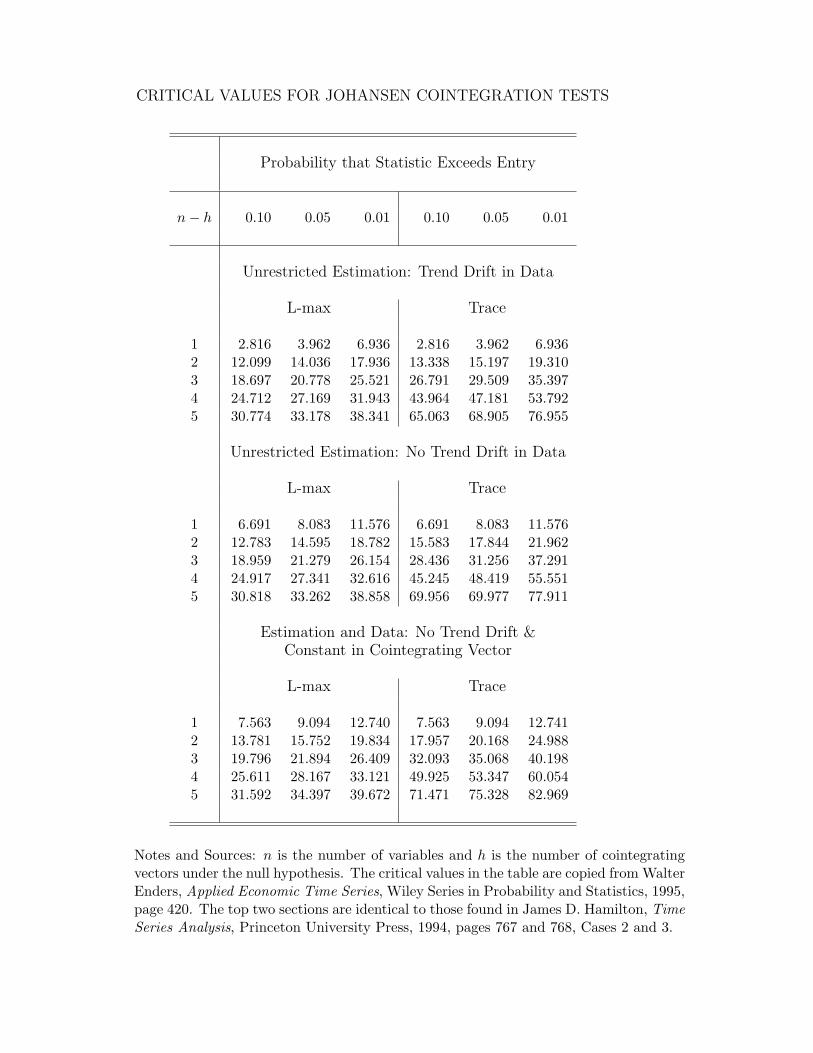
CRITICAL VALUES FOR JOHANSEN COINTEGRATION TESTS
Probability that Statistic Exceeds Entry
n− h 0.10 0.05 0.01 0.10 0.05 0.01
Unrestricted Estimation: Trend Drift in Data
L-max Trace
1 2.816 3.962 6.936 2.816 3.962 6.9362 12.099 14.036 17.936 13.338 15.197 19.3103 18.697 20.778 25.521 26.791 29.509 35.3974 24.712 27.169 31.943 43.964 47.181 53.7925 30.774 33.178 38.341 65.063 68.905 76.955
Unrestricted Estimation: No Trend Drift in Data
L-max Trace
1 6.691 8.083 11.576 6.691 8.083 11.5762 12.783 14.595 18.782 15.583 17.844 21.9623 18.959 21.279 26.154 28.436 31.256 37.2914 24.917 27.341 32.616 45.245 48.419 55.5515 30.818 33.262 38.858 69.956 69.977 77.911
Estimation and Data: No Trend Drift &Constant in Cointegrating Vector
L-max Trace
1 7.563 9.094 12.740 7.563 9.094 12.7412 13.781 15.752 19.834 17.957 20.168 24.9883 19.796 21.894 26.409 32.093 35.068 40.1984 25.611 28.167 33.121 49.925 53.347 60.0545 31.592 34.397 39.672 71.471 75.328 82.969
Notes and Sources: n is the number of variables and h is the number of cointegratingvectors under the null hypothesis. The critical values in the table are copied from WalterEnders, Applied Economic Time Series, Wiley Series in Probability and Statistics, 1995,page 420. The top two sections are identical to those found in James D. Hamilton, TimeSeries Analysis, Princeton University Press, 1994, pages 767 and 768, Cases 2 and 3.