Status of PSF Reconstruction at Lick

Mike Fitzgerald

Workshop on AO PSF ReconstructionMay 10-12, 2004

Quick Outline

● Recap Lick AO system's features● Reconstruction approach● Implementation issues● Calibration● Current performance● Future work

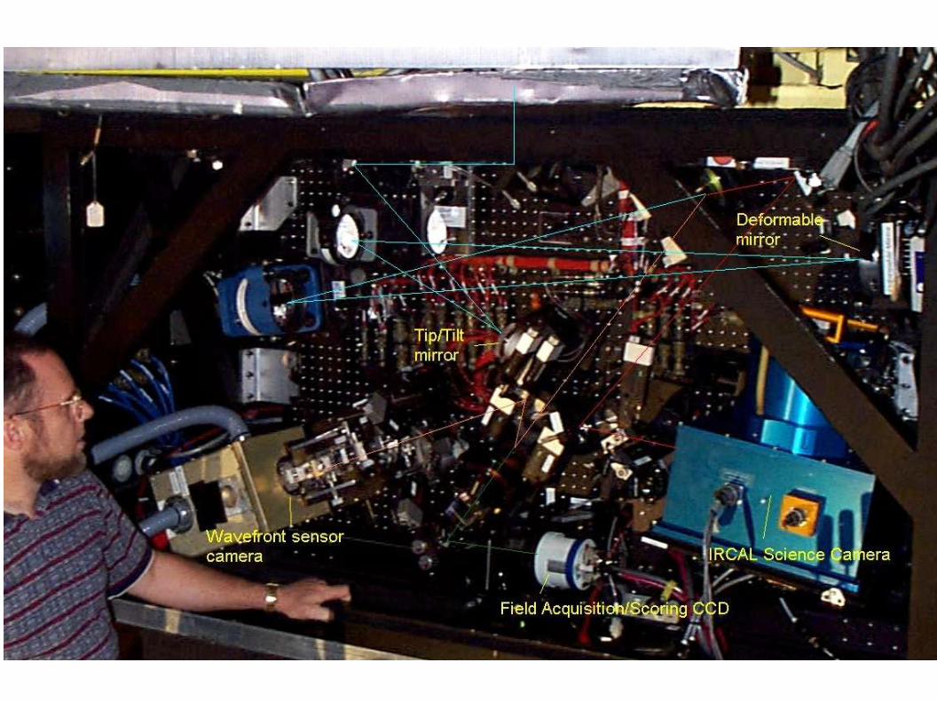
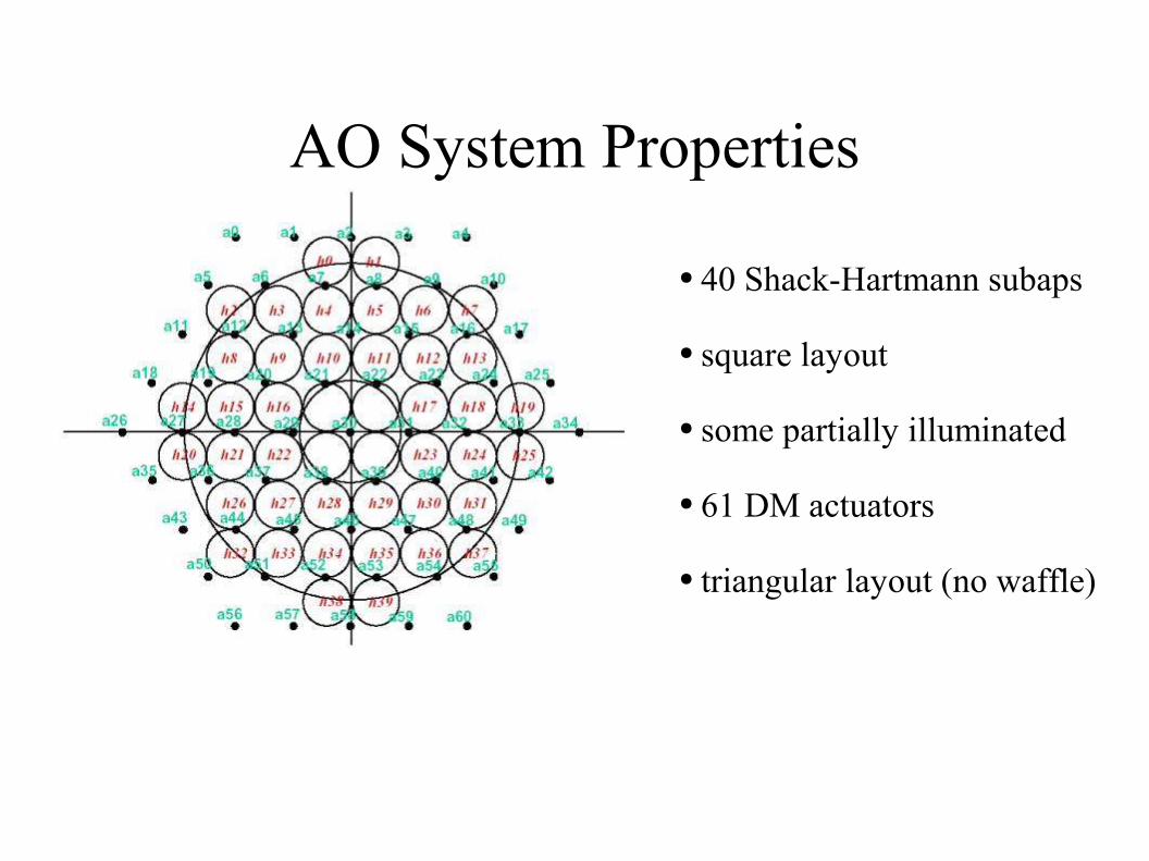
● 40 Shack-Hartmann subaps

● square layout

● some partially illuminated

● 61 DM actuators

● triangular layout (no waffle)

AO System Properties

AO System Properties

● Up to 1 kHz operation, 500 Hz typical

● Weighted-Least-Squares control matrix

● Laser Guide Star mode

● IRCAL camera Nyquist at 2.2 μm

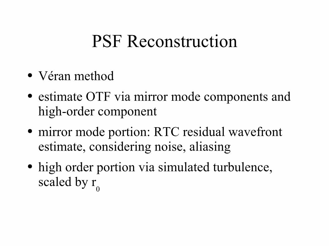
PSF Reconstruction

● Véran method● estimate OTF via mirror mode components and

high-order component● mirror mode portion: RTC residual wavefront

estimate, considering noise, aliasing● high order portion via simulated turbulence,

scaled by r0

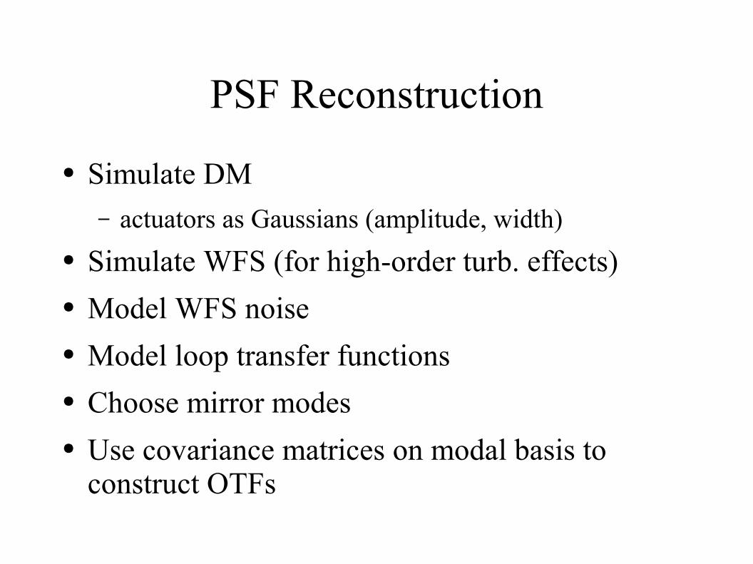
PSF Reconstruction

● Simulate DM– actuators as Gaussians (amplitude, width)

● Simulate WFS (for high-order turb. effects)● Model WFS noise● Model loop transfer functions● Choose mirror modes● Use covariance matrices on modal basis to

construct OTFs

More on Data Collection

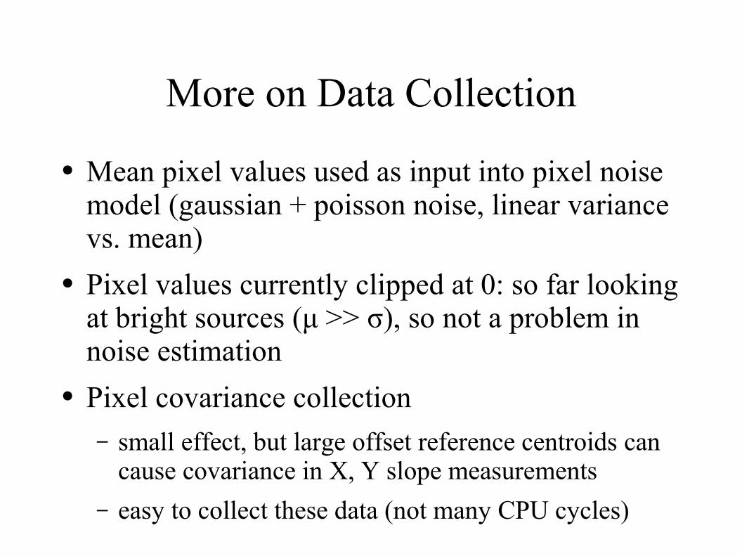
● Mean pixel values used as input into pixel noise model (gaussian + poisson noise, linear variance vs. mean)

● Pixel values currently clipped at 0: so far looking at bright sources (μ >> σ), so not a problem in noise estimation

● Pixel covariance collection– small effect, but large offset reference centroids can

cause covariance in X, Y slope measurements

– easy to collect these data (not many CPU cycles)

WFS Noise

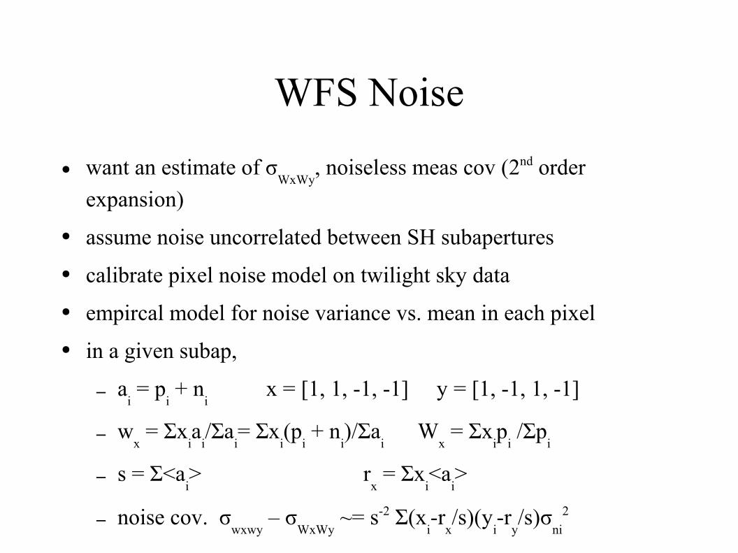
● want an estimate of σWxWy

, noiseless meas cov (2nd order

expansion)

● assume noise uncorrelated between SH subapertures

● calibrate pixel noise model on twilight sky data

● empircal model for noise variance vs. mean in each pixel

● in a given subap,

– ai = p

i + n

i x = [1, 1, -1, -1] y = [1, -1, 1, -1]

– wx = Σx

ia

i/Σa

i= Σx

i(p

i + n

i)/Σa

i W

x = Σx

ip

i /Σp

i

– s = Σ<ai> r

x = Σx

i<a

i>

– noise cov. σwxwy

– σWxWy

~= s-2 Σ(xi-r

x/s)(y

i-r

y/s)σ

ni

2

Mirror Mode Selection

● Wavefront basis functions orthonormal over pupil● Restrict to space of wavefronts produced by

mirror● Further restrict to space of wavefronts to which

the WFS is sensitive● Some subapertures are less sensitive (partial pupil

obscuration)...

Mirror Mode Selection

● D is system interaction matrix (push matrix)● SVD of DTWD gives WFS modes in actuator

basis● Remove low SV directions in actuator space to

which WFS is insensitive (invisible WFS modes)● Construct spatial representation of visible WFS

modes with simulated actuator influence functions

Mirror Mode Selection

● Construct matrix of wavefront inner products (over pupil) of WFS modes

● Eigenvectors of this matrix are the mirror modes

Simulations

● 1000 phase screens (D/r0=1)

● subtract mirror mode component● Use mirror mode component covariance as

emprical values of Kolmogorov model in modal basis

● Use high-order component for structure f'n calc● Use WFS response to high-order component to

extract aliasing covariance

Implementation Considerations

● code in IDL/C, system glue in Python

● Uij function storage

– for N modes, N(N+1)/2 unique functions

– for 1282 pupil grid, 2562 OTF grid

– want in RAM

Calibration: DM

● Ideally one would have a map of OPD● Currently simulate influence functions with

gaussians, fit parameters to system interaction matrix D– couples with WFS simulation

– partially-illuminated subaps?

● voltage response temp. dependent - timescales?● need to improve this calibration

Calibration: WFS

● WFS scale– set by angular size of WFS detector pixels

– bootstrap with science camera scale

Calibration: WFS

● WFS spot gain– larger spot size reduces tilt sensitivity of subaps

– scale RTC estimate of Cεε by g

spot

-2 – large effect!

– try to measure:● take open-loop and closed-loop temporal power spectra.

ratio will give the correction transfer function Hcor

(f, geff

)

(disturbance rejection)● inject small tip/tilt dither, synchronous phase with WFS

readout (but smaller than diffraction limit)● other?

Calibration

● Control loop dynamics– delay is main unknown

● profile RTC code

● fit as parameter in Hcor

measurement (power spectra ratio)

● Lick: about 1.4 ms; significant for 1 kHz operation

● Quasi-static OTF– internal source (doesn't get primary/secondary aberr.)

– well-corrected on-sky measurements

– what are the variation timescales?

Performance

● 10 sec exposures of bright binary stars (mV ~ 7)● 1.5 to 4 arcsec separations● narrow-band (Brγ)● extract image PSF with Starfinder; normalize

with box 4.8 arcsec on a side (64 pixels)● Static OTF from internal source only

Performance

● Calibration problems affecting reconstructed PSF

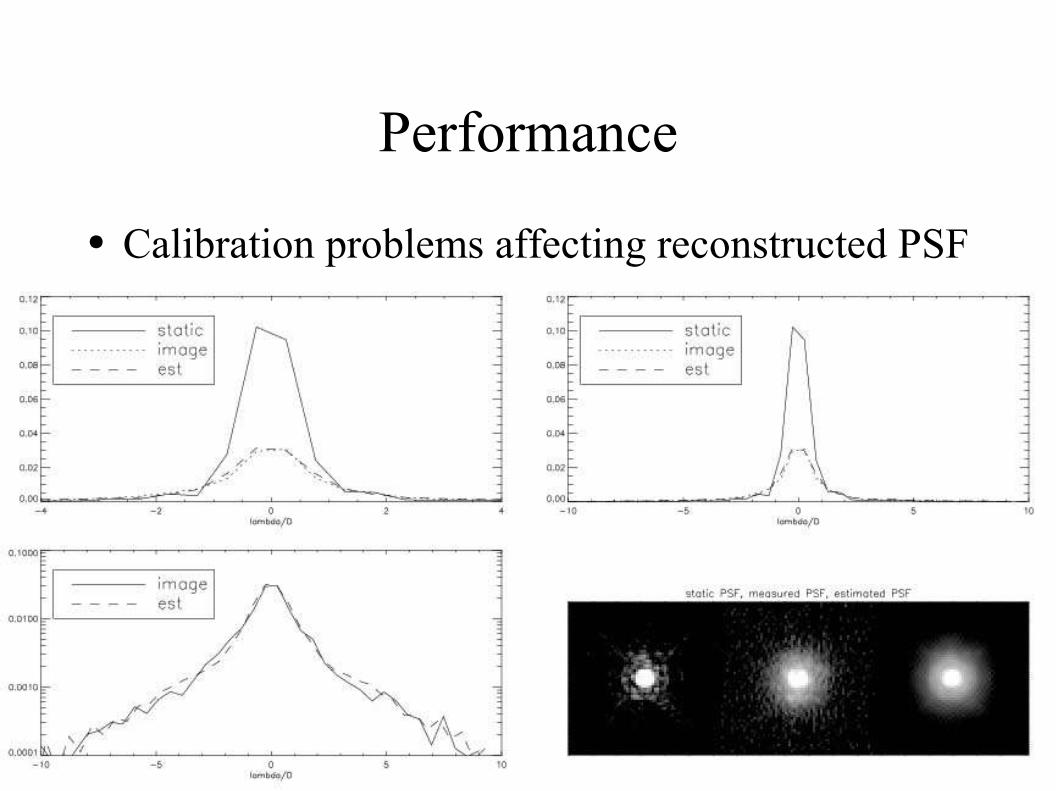
Performance

● Calibration problems affecting reconstructed PSF

Miscalibration

● How does miscalibration affect reconstructed PSF?

● Spot gain lowers estimate of residual phase from actual: overestimate Strehl

● DM scale affects r0 estimate. Bright sources have

aliasing as major component...

What's Next

● In-depth analysis of data set● How do we best calibrate our dominant error

sources?● Integrate other centroid routines (4x4,

correlation)● Integrate LGS mode TT sensor data