Stochastic Demand and Revealed Preference�

Richard Blundelly Dennis Kristensenz Rosa Matzkinx

This version: May 2010

Preliminary Draft

Abstract

This paper develops new techniques for the estimation and testing of stochastic consumer

demand models. For general non-additive stochastic demand functions, we demonstrate how

revealed preference inequality restrictions from consumer optimisation conditions can be utilized

to improve on the nonparametric estimation and testing of demand responses. We show how

bounds on demand reponses to price changes can be estimated nonparametrically, and derive

their asymptotic properties utilizing recent results on estimation and testing of parameters

characterized by moment inequalities. We also devise a test for rationality of the consumers.

An empirical application using data from the U.K. Family Expenditure Survey illustrates the

usefulness of the methods.

JEL: C20, D12

Keywords: micreconometrics, consumer behaviour, revealed preference, bounds, rationality.

�We would like to thank Ian Crawford and Roger Koenker for sharing Matlab code with us and helping with the

implementation. We also wish to thank participants at the Latin-American Meetings in Buenos Aires, the CAM

workshop at University of Copenhagen and at the Malinvaud Seminar for helpful comments and suggestions.yDepartment of Economcis, UCL. E-mail: r.blundell@ucl.ac.uk.zDepartment of Economics, Columbia University and CREATES. E-mail: dk2313@columbia.eduxDepartment of Economics, UCLA. E-mail: matzkin@econ.ucla.edu.

1

1 Introduction

This paper develops new nonparametric techniques for the estimation and prediction of consumer

demand responses. The objectives are two-fold: First, to impose minimum restrictions on how

unobserved heterogeneity enters the demand function of the individual consumer. Second, to utilize

restrictions arriving from choice theory to improve demand estimation and prediction.

Our analysis takes place in the commonly occurring empirical setting where only a relatively

small number of market prices are observed, but within each of those markets the demand responses

of a large number of consumers are reported. In this setting, it is not possible to point identify the

predicted demand response to a new, unobserved price. We will instead use restrictions derived

from revealed preference theory to establish bounds on the demand responses: If consumers behave

according to the axioms of revealed preference their vector of demands at each relative price will

satisfy certain well known inequalities (see Afriat, 1973 and Varian, 1982). If, for any individual,

these inequalities are violated then that consumer can be deemed to have failed to behave according

to the optimisation rules of revealed preference. In this paper, we will employ the results of

Blundell, Browning and Crawford (2003, 2008) who extend the analysis of Varian (1982) and

obtain �expansion path based bounds�(E-bounds) which are the tightest possible bounds, given the

data and the theory. These restrictions will be used to obtain improved quantile demand estimates

at observed prices, and to establish bounds on the predicted distribution of demands at new prices.

We �rst develop nonparametric sieve estimators of the stochastic demand functions at any given

set of observed prices, and show how revealed preferences can be imposed in the estimation. In the

estimation, we impose weak assumptions on how the unobserved heterogeneity enters the demand

function. In particular, we allow for non-additive heterogeneity which is in contrast to most of the

existing literature on the estimation of Engel curves. We show how the estimator can be formulated

as a constrained nonparametric quantile estimation problem, and derive its asymptotic properties.

The second part of the paper is concerned with predicting consumer demand responses to a new

relative price level that has not been previously observed. Given the limited price variation it is not

possible to nonparametrically point identify demand at new, previously unobserved, relative prices.

However, the revealed preference restrictions developed in Blundell, Browning and Crawford (2003,

2008) allow us to establish bounds on the demands for the nonseparable heterogeneity case that is

the focus here. We show how the demand functions estimated at observed prices, can be used to

recover these bounds nonparametrically. The estimation problem is non-standard and falls within

the framework of partially identi�ed models (see e.g. Manski, 1993). We employ the techniques

developed in, amongst others, Chernozhukov, Hong and Tamer (2003) to establish the properties

of the nonparametric demand bounds estimators. As in that part of the literature, the asymptotic

distribution is non-standard and con�dence bands can in general not be computed directly.

The estimation and prediction strategy outlined above heavily exploits revealed preference in-

equalities. In the third part of the paper, we develop a nonparametric test for this rationality

assumption. This testing problem is again non-standard since the testable restrictions take the

form of a set of inequality constraints. As such the testing problem is similar to one of estimation

2

and testing when the parameter is on the boundary of the parameter space as analyzed in, for

example, Andrews (1999, 2001) and Andrews and Guggenberger (2009). By importing the tech-

niques developed there, we derive the asymptotic properties of the test statistic. Again, this is

highly non-standard and requires the use of either simulations or resampling techniques.

Our empirical analysis is based on data from the U.K. Family Expenditure Survey where the

relative price variation occurs over time, and samples of consumers, each of a particular household

type, are observed at speci�c points in time in particular regional locations. Employing the devel-

oped methodology, we obtain demand function and E-bounds estimates for own- and cross-price

demand responses using these expansion paths. We �nd that it is indeed important to relax the

additive restriction normally imposed in empirical consumer demand analysis, and that the bounds

are informative.

A key ingredient of the analysis we conduct is the Engel curve which describes the expansion

path for demand as total expenditure changes. The modelling and estimation of this relationship has

a long history. Working (1943) and Leser (1963) suggested standard parametric regression models

where budget shares are linear functions of log total budget; the so-called Piglog-speci�cation.

This simple linear model has since then been generalised in various ways since empirical studies

suggested that higher order logarithmic expenditure terms are required for certain expenditure

share equations, see e.g. Hausman, Newey and Powell (1995), Lewbel (1991), Banks, Blundell and

Lewbel (1997). An obvious way to detect the presence of such higher order terms is non- and

semiparametric methods which have been widely used in the econometric analysis of Engel curves,

see for example Blundell, Chen and Kristensen (2007), Blundell and Duncan (1998) and Härdle

and Jerison (1988).

In most of these empirical studies it has been standard to simply impose an additive error

structure which greatly facilitates the econometric analysis since the demand model collapses to

a regression. This type of speci�cation allows relatively straightforward identi�cation and estima-

tion of the structural parameters. Additive heterogeneity on the other hand imposes very strong

assumptions on the class of underlying utility functions, see e.g. Lewbel (2001), and as such is in

general inconsistent with economic theory; see also Beckert (2007). In response to this problem

with existing empirical consumer demand models, we allow for non-additive heterogeneity struc-

tures thereby allowing for observed and unobserved characteristics to interact in a much more

involved manner compared to standard additive speci�cations. See Lewbel and Pendakur (2009)

for one of the few parametric speci�cation that allows non-additive interaction.

An early treatment of nonparametric identi�cation of non-additive models is Brown (1983)

whose results were extended in Roehrig (1988). Brown and Matzkin (1998, 2003) and Matzkin

(2003a,b) building on their work propose estimators. A number of other papers have addressed

identi�cation and estimation: Chesher (2001, 2002a, 2002b, 2003) consider quantile-driven identi�-

cation; Ma and Koenker (2003) make use of his results to construct parametric estimators; Imbens

and Newey (2009) and Chernozhukov, Imbens and Newey (2003) establish estimators which allow

for endogeneity. Our unconstrained demand function estimator is similar to the ones developed in

Imbens and Newey (2009).

3

An important feature of the estimation of Engel curve is the possible presence of endogeneity

in the total expenditure variable. In a parametric framework this can be dealt with using stan-

dard IV-techniques. In recent years, a range of di¤erent methods have been proposed to deal with

this problem in a nonparametric setting. The two main approaches proposed in the literature is

nonparametric IV (Ai and Chen (2003), Hall and Horowitz (2003), Darolles, Florens and Renault

(2002)) and control functions (Newey, Powell and Vella (1998)). Both these methods have been

applied in the empirical analysis of Engel curves (Blundell, Chen and Kristensen (2003) and Blun-

dell, Duncan and Pendakur (1998) respectively). We brie�y discuss how our estimators and tests

can be extended to handle endogeneity of explanatory variables by using recent results in Chen

and Pouzo (2009), Chernozhukov, Imbens and Newey (2007) and Imbens and Newey (2009).

Finally, we note that other papers have combined nonparametric techniques and economic

theory to estimate and test demand systems; see, for example, Haag, Hoderlein and Pendakur

(2009), Hoderlein (2008), Hoderlein and Stoye (2009), Lewbel (1995).

The remainder of the paper is organized as follows: In Section 2, we set up the basic econometric

framework. In Section 3-4, we develop estimators of the demand functions at observed prices. The

estimation of demand bounds is considered in Section 5, while a test for rationality is developed

in Section 6. In Sections 7 and 8, we discuss the implementation of the estimators and how to

compute con�dence bands. We brie�y discuss how to allow for endogenous explanatory variables

in Section 9. Section 10 contains an empirical application on British household data. We conclude

in Section 11. All proofs have been relegated to the Appendix.

2 The Framework

Suppose we have observed a consumers�market over T periods. Let p (t) be the set of prices for

the goods that all consumers face at time t = 1; :::; T . At each time point t, we draw a new random

sample of n � 1 consumers. For each consumer, we observe his demands and income level (and

potentially some other characteristics such as age, education etc.). Let qi (t) and xi (t) be consumer

i�s (i = 1; :::; n) vector of demand and income level at time t (t = 1; :::; T ). We stress that the data

fp (t) ;qi (t) ; xi (t)g, t = 1; :::; T and i = 1; :::; n, is not a panel data set since we do not observe thesame consumer over time.

We focus on the situation where there are only two goods in the economy such that q (t) =

(q1 (t) ; q2 (t))0 2 R2+ and p (t) = (p1 (t) ; p2 (t))

0 2 R2+.1 The demand for good 1 is assumed to arrivefrom the following demand function,

q1 (t) = d1 (x (t) ;p (t) ; " (t)) ;

where " (t) 2 R is an individual speci�c error term that may re�ect individual heterogeneity in

preferences (tastes). To ensure that the budget constraint is met, the demand for good two must

1By the end of the paper, we discuss extensions to general, multidimensional goods markets.

4

satisfy:

q2 (t) = d2 (x (t) ;p (t) ; " (t)) :=x (t)� p1 (t) d1 (x (t) ;p (t) ; " (t))

p2 (t):

We collect the two demand functions in d = (d1; d2). The demand function d should be thought of

as the solution to an underlying utility maximization problem that the individual consumer solves.

The demand function could potentially depend on other observable characteristics besides in-

come, but to keep the notation at a reasonable level we suppress such dependence in the following.

If additionally explanatory variables are present, all the following assumptions, arguments and

statements are implicitly made conditionally on those.

We here consider the often occurring situation where the time span T over which we have

observed consumers and prices is small (in the empirical application T = 6). In this setting, we do

not observe enough price variation to identify how these impact demand; thus, we are not able to

identify the mapping p 7! d (x;p; "). To emphasize this, we will in the following write

d (x (t) ; t; " (t)) := d (x (t) ;p (t) ; " (t)) :

So we have a sequence of T demand functions, fd (x; t; ")gTt=1.The unobserved heterogeneity " (t) is assumed (or normalized) to follow a uniform distribution,

" (t) � U [0; 1] and to be independent of x (t).2 This combined with the assumption that d1 is

invertible in " (t) implies that d1 (x; t; �) is identi�ed as the �th quantile of q1 (t) jx (t) = x (Matzkin,2003; Newey and Imbens, 2009):

d1 (x; t; �) = F�1q1(t)jx(t)=x (�) ; � 2 [0; 1] : (1)

3 Unrestricted Sieve Estimator

We here develop sieve estimators of the sequence of demand functions d (x; t; ") = (d1 (x; t; ") ; d2 (x; t; ")),

t = 1; :::; T .

As a starting point, we assume that for all t = 1; :::; T and all � 2 [0; 1], the function x 7!d1 (x; t; �) is situated in some known function space D1 which is equipped with some (pseudo-)norm k�k.3 We specify the precise form of D1 and k�k below. Given the function space D1, wechoose sieve spaces D1;n that are �nite-dimensional subsets of D. In particular, we will assumethat for any function d1 2 D1, there exists a sequence �nd1 2 D1;n such that k�nd1 � d1k ! 0 as

n!1. Most standard choices of the function space D1 can be written on the form

D1 =(d1 : d1 (x; t; �) =

Xk2K

�k (t; �)Bk (x) ; � (t; �) 2 RjKj);

2The independence assumption can be relaxed as discussed in Section 9.3The function space could without problems be allowed to depend on time, t, and the errors, � . For notational

simplicity, we maintain that the function space is the same across di¤erent values of (t; �).

5

for known (basis) functions fBkgk2K, and some (in�nite-dimensional) index set K; see Chen (2007,Section 2.3) for some standard speci�cations. A natural choice for sieve is then

D1;n =

8<:dn;1 : dn;1 (x; t; �) = Xk2Kn

�k (t; �)Bk (x) ; � (t; �) 2 RjKnj9=; ; (2)

for some sequence of (�nite-dimensional) sets Kn � K. Finally, we de�ne the space of vector

functions,

D =�d = (d1; d2) : d1 (x; t; �) 2 D1; d2 (t; x; �) :=

x� p1 (t) d1 (x; t; �)p2 (t)

�;

and with the associated sieve space Dn de�ned similarly to D1;n.Given the function space D and its associated sieve, we can construct a sieve estimator of the

function d (�; t; �). Given that d1 (x; t; �) is identi�ed as a conditional quantile for any given valueof x, c.f. eq. (1), we may employ standard quantile regression techniques to obtain the estimator:

Let

�� (z) = (I fz < 0g � �) z; � 2 [0; 1] ;

be the standard check function used in quantile estimation (see Koenker and Bassett, 1978). We

then propose to estimate d (x; t; �) by

d (�; t; �) = arg mindn2Dn

1

n

nXi=1

�� (q1;i (t)� dn;1 (xi (t) ; t; �)) ; (3)

for any t = 1; :::; T and � 2 [0; 1].The above estimator can be computed using standard numerical methods for linear quantile

regressions when the sieve space is on the form in Eq. (2): De�ne Wi (t) = fBk (xi (t)) : k 2 Kng 2RjKnj as the collection of basis functions spanning the sieve D1;n. Then the sieve estimator is givenby d1 (x; t; �) =

Pk2Kn �k (t; �)Bk (x), where

� (t; �) = arg min�2RjKnj

1

n

nXi=1

���q1;i (t)� �0Wi (t)

�; � 2 [0; 1] : (4)

That is, the estimator � (t; �) is simply the solution to a standard linear quantile regression problem.

Finally, the estimator of the demand function for the "residual" good is given by

d2 (x; t; �) =x� p1 (t) d1 (x; t; �)

p2 (t): (5)

To develop an asymptotic theory of the proposed sieve estimator, the following assumptions are

imposed on the model:

A.1 Income x (t) has bounded support, x (t) 2 X = [a; b] for �1 < a < b < +1, and isindependent of " � U [0; 1].

A.2 The demand function d1 (x; t; ") is invertible in " and is continuously di¤erentiable in (x; ").

6

These are fairly standard assumptions in the literature on nonparametric quantile estimation.

It would be desirable to weaken the restriction of bounded support, but the cost would be more

complicated conditions and proof so we maintain (A.1) (see e.g. Chen, Blundell and Kristensen,

2007 for results with unbounded support). The independence assumption rules out endogenous

income; in Section 9, we argue how this can be allowed for by adopting nonparametric IV or

control function approaches. We refer to Beckert (2007) and Beckert, and Blundell (2008) for more

primitive conditions in terms of the underlying utility-maximization problem for (A.2) to hold.

We restrict our attention to the case where either B-splines or polynomial splines are used to

construct the sieve space D1;n. For an introduction to these, we refer to Chen (2007, Section 2.3).All of the following results remain true with other linear sieve spaces after suitable modi�cations

of the conditions. We introduce the following L2- and sup-norms which will be used to state our

convergence rate results:

jjdjj2 =pE [kd (x; t; �)k]; jjdjj1 = sup

x2Xkd (x; t; �)k :

The function space D1 is then restricted to satisfy:

A.3 The function d1 (�; t; �) 2 D1, where D1 = Wm2 ([a; b]) and Wm

2 ([a; b]) is the Sobolev space of

all functions on [a; b] with L2-integrable derivatives up to order m � 0.

We now have the following result:

Theorem 1 Assume that (A.1)-(A.3) hold. Then for any t = 1; :::; T and � 2 [0; 1]:

jjd (�; t; �)� d0 (�; t; �) jj2 = OP (pkn=n) +OP

�k�mn

�In particular, with kn = O

�n1=(2m+1)

�,

jjd (�; t; �)� d0 (�; t; �) jj2 = OP�nm=(2m+1)

�:

The above convergence result is established in the L2-norm. For later use, we note that in the

sup-norm it holds that (see Chen and Liao, 2009):

jjd (�; t; �)� d0 (�; t; �) jj1 = OP (kn=pn) +OP

�k�mn

�:

This is helpful when developing the asymptotic properties of the constrained estimator.

To establish the asymptotic distribution of our sieve estimator, we employ the results of Chen

and Liao (2009) and obtain:

Theorem 2 Assume that (A.1)-(A.3) hold; the smallest eigenvalue of E�Bkn (x)Bkn (x)

0� is boundedand bounded away from zero; k4n=n = O (1) and k3m�1=2n =n = O (1). Then for any x (t) 2 X ,t = 1; :::; T , and � 2 [0; 1],

�1=2n (x; �)

0BB@d (x (1) ; 1; �)� d0 (x (1) ; 1; �)

...

d (x (T ) ; T; �)� d0 (x (T ) ; T; �)

1CCA!d N (0; I) ;

where �n (x; �) is given in Chen and Liao (2009).

7

A consistent estimator of �n (x; �) is

�n (x; �) = ::::

4 GARP-Restricted Sieve Estimator

We now wish to impose revealed preferences (GARP) restrictions on the function d in the esti-

mation. First, we brie�y introduce the concept of GARP; see Blundell, Browning and Crawford

(2003, 2008) for a more detailed introduction to GARP and its empirical implications.

Consider a given income level x (T ) at time T , and compute recursively for t = T �1; T �2; :::1,an income expansion path fx (t)g by

x (t) = p (t)0 d (x (t+ 1) ; t+ 1; �) :

We then require that the demand of a given consumer characterised by � 2 [0; 1] satis�es:

p (t)0 d (x (t) ; t; �) = x (t) � p (t)0 d (x (s) ; s; �) ; s < t, t = 2; :::; T: (6)

If the demand functions d (x; t; �), t = 1; :::; T , satisfy these inequalities for any given income level

x (T ) we say that "d satis�es GARP".

We expect that if indeed the consumers in our sample satisfy GARP, more precise estimates

of d (�; �; �) can be obtained by imposing this restriction. Furthermore, once a GARP restrictedestimator has been obtained, it can be used to test for GARP by comparing it with the unrestricted

estimator developed in the previous section. A GARP-restricted sieve estimator is easily obtained

in principle: First observe that the unrestricted estimator of fd (�; t; �)gTt=1 of the previous sectioncan be expressed as the solution to the following joint estimation problem.

fd (�; t; �)gTt=1 = arg minfdn(�;t;�)gTt=12DTn

1

n

TXt=1

nXi=1

�� (q1;i (t)� d1;n (t; xi (t))) ; � 2 [0; 1] ;

where DTn = Tt=1Dn and Dn is de�ned in the previous section. Since there are no restrictions acrossgoods and t, the above de�nition of fd (�; t; �)gTt=1 is equivalent to the unrestricted estimators ineqs. (3) and (5). In order to impose the GARP restrictions, we simply de�ne the constrained

function set as

DTC := DT \ fd (�; �; �) satis�es GARPg ; (7)

and similarly the constrained sieve as

DTC;n := DTn \ fdn (�; �; �) satis�es GARPg :

We de�ne the constrained estimator by:

fdC (�; t; �)gTt=1 = arg minfdn(�;t;�)gTt=12DTC;n

1

n

TXt=1

nXi=1

�� (q1;i (t)� d1;n (t; xi (t))) ; � 2 [0; 1] : (8)

8

Since GARP imposes restrictions across both goods (l = 1; 2) and time (t = 1; :::; T ), the above

estimation problem can no longer be split up into individual subproblems as in the unconstrained

case.

The proposed estimator shares some similarities with the ones considered in, for example,

Berestenau (2004), Gallant and Golub (1984), Mammen and Thomas-Agnan (1999) and Yatchew

and Bos (1997) who also consider constrained sieve estimators. However, they focus on least-

squares regression while ours is a least-absolute deviation estimator, and they furthermore restrict

themselves to linear constraints. There are some results for estimation of monotone quantiles and

other linear constraints, see Chernozhukov et al (2006), Koenker and Ng (2005) and Wright (1984),

but again their constraints are simpler to analyze and implement. These two issues, a non-smooth

criterion function and non-linear constraints, complicate the analysis and implementation of our

estimator, and we cannot readily import results from the existing literature.

In order to derive the convergence rate of the constrained sieve estimator, we employ the same

proof strategy as found elsewhere in the literature on nonparametric estimation under shape con-

straints, see e.g. Birke and Dette (2007), Mammen (1991), Mukerjee (1988): We �rst demonstrate

that as n ! 1, the unrestricted estimator, d, satis�es GARP almost surely. This implies thatfd (�; t; �)gTt=1 2 DTC;n with probability approaching one (w.p.a.1) which in turn means that d = dCw.p.a.1, since dC solves a constrained version of the minimization problem that d is a solution

to. We are now able to conclude that dC is asymptotically equivalent d, and all the asymptotic

properties of d are inherited by dC .

For the above argument to go through, we need to slightly change the de�nition of the con-

strained estimator though. We introduce the following generalized version of GARP: We say that

"d satis�es GARP(�)" for some ("small") � � 0 if for any income expansion path,

x (t) � p (t)0 d (x (s) ; s; �) + �; s < t, t = 2; :::; T:

The de�nition of GARP(�) is akin to Afriat (1973) who suggests a similar modi�cation of GARP

to allow for waste ("partial e¢ ciency"). We then de�ne the constrained function space and its

associated sieve as:

DTC (�) = DT \ fd (�; �; �) satis�es GARP (�)g ;

DTC;n (�) = DTn \ fdn (�; �; �) satis�es GARP (�)g :

We note that the constrained function space DTC as de�ned in eq. (7) satis�es DTC = DTC (0).Moreover, it should be clear that DTC (0) � DTC (�) and DTC:n (0) � DTC;n (�) since GARP(�), � > 0,imposes weaker restrictions on the demand functions.

We now re-de�ne our GARP constrained estimators to solve the same optimization problem as

before, but now the optimization takes place over DC;n (�). We let d�C denote this estimator, andnote that d0C = dC , where dC is given in Eq. (8). The assumption that fd0 (�; t; �)g

Tt=1 2 DTC (0)

implies that fd (�; t; �)gTt=1 2 DTC;n (�) w.p.a.1. Since d�C is a constrained version of d, this impliesthat d�C = d w.p.a.1. Similar assumptions and proof strategies have been employed in Birke

and Dette (2007) [Mammen (1991)]: They assume that the function being estimated is strictly

9

convex [monotone], such that the unconstrained estimator is convex [monotone] w.p.a.1. Since

DTC;n (0) � DTC;n (�), our new estimator will in general be less precise than the one de�ned as theoptimizer over DTC;n (0), but for small values of � > 0 the di¤erence should be negligible.

Theorem 3 Assume that (A.1)-(A.3) hold, and that d0 2 DTC (0). Then for any � > 0:

jjd�C (�; t; �)� d0 (�; t; �) jj1 = OP (kn=pn) +OP

�k�mn

�;

for t = 1; :::; T . Moreover, the estimator has the same asymptotic distribution as the unrestricted

estimator given in Theorem 2.

It should be noted that in terms of convergence rate our unconstrained and constrained esti-

mators are asymptotically equivalent. In terms of asymptotic convergence rate, we are not able

to show that our additional constraints lead to an improvement of the estimator. This is simi-

lar to other results in the literature on constrained nonparametric estimation. Kiefer (1982) and

Berestenau (2004) establish optimal nonparametric rates in the case of constrained densities and

regression functions respectively when the constraints are not binding. In both cases, the optimal

rate is the same as for the unconstrained one. However, as demonstrated both analytically and

through simulations in Mammen (1991) for monotone restrictions (see also Berestenau, 2004 for

simulation results for other restrictions), there may be signi�cant �nite-sample gains.

We conjecture that the above result will not in general hold for the estimator dC de�ned as

the minimizer over DTC;n (0). In this case the GARP constraints would be binding, and we canno longer ensure that the unconstrained estimator is situated in the interior of the constrained

function space. This in turn means that the unconstrained and constrained estimator most likely

are not asymptotically equivalent and very di¤erent techniques have to be used to analyze the con-

strained estimator. In particular, the rate of convergence and/or asymptotic distribution of it would

most likely be non-standard. This is, for example, demonstrated in Andrews (1999,2001), Anevski

and Hössjer (2006) and Wright (1981) who give results for inequality-constrained parametric and

nonparametric problems respectively.

Finally, we note that the above theorem is not speci�c to our particular quantile sieve estimator.

One can by inspection easily see that the arguments employed in our proof can be carried over

without any modi�cations to show that for any unconstrained demand function estimator, the

corresponding RP-constrained estimator will be asymptotically equivalent.

5 Estimation of Demand Bounds

Once an estimator of the demand function has been obtained, either unrestricted or restricted,

we can proceed to estimate the associated demand bounds. We will here utilize the machinery

developed in Chernozhukov, Hong and Tamer (2007) and use their results to develop the asymptotic

theory of the proposed demand bound estimators.

Consider a particular consumer characterized by some � 2 [0; 1] with associated sequence ofdemand functions d (x; t; �), t = 1; :::; T . Since we keep � �xed, we suppress the dependence of this

10

variable in the following. Suppose that the consumer faces a given new price p0 at an income level

x0. De�ne the consumer�s budget set as

Bp0;x0 =�q 2 R2+jp00q = x0

;

which is compact and convex. The closure of consumer�s so-called demand support set can then be

represented as follows:

Sp0;x0 =�q 2 Bp0;x0 jp (t)

0 q � p (t)0 d(x (t) ; t; �); t = 1; :::; T;

where fx (t)g solvesp00d(x (t) ; t; �) = x0; t = 1; :::; T:

A natural estimator is then to simply substitute the estimated demand functions for the unknown

ones. De�ne fx (t)g as the solution to

p00dC(x (t) ; t; �) = x0; t = 1; :::; T:

We then de�ne the estimator of the support set as

Sp0;x0 (c) =�q 2 Bp0;x0 jp (t)

0 q � p (t)0 dC(x (t) ; t; �)� c=n; t = 1; :::; T;

for some positive sequence c ! 1 with c=n ! 0. In order to do inference, we wish to choose a

(possibly data dependent) sequence c such that

P (Sp0;x0 � Sp0;x0 (c))! 1� �;

for some given con�dence level 1��. Here, we need to choose c > 0 to obtain the correct coverage,even if S (0) is consistent.

To derive the asymptotic properties of Sp0;x0 (c), we employ the general results of Chernozhukov,Hong and Tamer (2007). To see how our estimator �ts into their general framework, de�ne the

following set of "moments" m (q),

m (q) = �Pq+ b; m (q) = �Pq+ b;

where q 2 R2,P = [p (1) ; � � � ;p (T )]0 2 RT�2+ ; (9)

and

b =�p (1)0 d(x (1) ; 1; �); � � � ;p (T )0 d(x (T ) ; T; �)

�0; b =

hp (1)0 dC(x (1) ; 1; �); � � � ;p (T )0 dC(x (T ) ; T; �)

i0We can then express Sp0;x0 and Sp0;x0 (c) in terms of a set of moment inequalities:

Sp0;x0 = fq 2 Bp0;x0 jm (q) � 0g ; Sp0;x0 (c) = fq 2 Bp0;x0 jm (q) � c=ng :

11

The asymptotic results for Sp0;x0 (c) will be stated in terms of the Hausmann norm given by:

dH(A1;A2) = max(supy2A1

�(y;A2); supy2A2

�(y;A1)), � (y;A) = inf

x2Akx� yk ,

for any two sets A1;A2 2 R2. We impose the following additional condition:s are imposed on thedemand functions d and the observed prices p:

A.4 x (t) 7! d (x (t) ; t; �) is monotonically increasing, t = 1; :::; T .

A.5 The matrix P 2 RT�2+ de�ned in Eq. (9) has rank 2.

Theorem 4 Assume that (A.1(-(A.5) hold. Then for any sequence c / log (n),

dH(Sp0;x0 (c) ;Sp0;x0) = OP (plog (n) =rn):

Also,

P (Sp0;x0 � Sp0;x0 (c))! 1� �;

where c = c1��+OP (log (n)) with c1�� being an estimator of (1� �)th quantile of Qp0;x0 given by

Qp0;x0 := supq2Sp0;x0

kZ (y) + � (y)k2+ :

Here, q 7! Z (q) is a zero-mean Gaussian process with covariance matrix

� (q1;q2) =

q01 IT OT�T

OT�2T �IT

! O O

O

! q2 IT O2T�T

OT�T �IT

!;

with

= P (I2T ; I2T )� (x; �)0 (I2T ; I2T )

0 P 0;

where is given in Eq. (25), while � (q) = (�1 (q) ; :::; �T (q))0 is given by

�t (q) =

(�1; p (t)0 q > p (t)0 d(x (t) ; t; �)

0; p (t)0 q = p (t)0 d(x (t) ; t; �); t = 1; :::; T:

In order to employ the above result, one either have to simulate the asymptotic distribution

by Monte Carlo methods, or use resampling methods. In the latter case, one can either use the

modi�ed bootstrap procedures developed in Bugni (2009,2010) and Andrews and Soares (2010) or

the subsampling procedure of Chernozhukov, Hong and Tamer (2007); we discuss in more detail in

Section 8 how the bootstrap procedure of Bugni (2009,2010) can be implemented in our setting.

12

6 Testing for Rationality

In the previous two sections, we have developed estimators of the demand responses under revealed

preferences constraints. It is of interest to test whether the consumers in the data set indeed do

satisfy these restrictions: First, from an economic point of view it is highly relevant to test the

axioms underlying standard choice theory. Second, from an econometric point of view, we wish to

test whether the imposed constraints are actually satis�ed in data.

We here develop a test for whether the consumers satisfy the revealed preference aximom;

that is, are they rational? A natural way of testing this hypothesis would be to compare the

unrestricted and restricted demand function estimates, and rejecting if they are "too di¤erent"

from each other. Unfortunately, since we have only been able to develop the asymptotic properties

of the constrained estimator under the hypothesis that none of the inequalities are binding, the

unrestricted and restricted estimators are asymptotically equivalent under the null. Thus, any

reasonable test comparing the two estimates would have a degenerate distribution under the null.

Instead, we take the same approach as in Blundell et al (2008) and develop a minimum-distance

statistic. For given price and income levels p0 and x0, de�ne the associated intersection demands,

q (p0; x0; t; �) = d (x (t) ; t; �) 2 R2; (10)

where d is the unrestricted demand function estimator, and fx (t)g solves

p00d(x (t) ; t; �) = x0; t = 1; :::; T: (11)

We then introduce the following statistic to measure discrepancies between a given alternative set

of demands, q = (q (1) ; :::;q (T )) 2 R2T , and q:

MDn�qjp0; x0; �

�=

TXt=1

(q (t)� q (p0; x0; t; �))0Wt (q (t)� q (p0; x0; t; �)) ;

where Wt 2 R2�2 is some weighting matrix; it could for example be chosen as an estimator of theinverse of the asymptotic covariance matrix of q (p0; x0; t; �) as given in Theorem 2. We then de�ne

the projection of the unrestricted demand prediction as:

q� = arg minq2Sp0;x0

MDn�qjp0; x0; �

�;

where Sp0;x0 is the set of intersection demands that satisfy GARP. As demonstrated in Blundell etal (2008), this can be written as:

Sp0;x0 =�q 2 BTp0;x0

��9V > 0; � � 1 : Vt � Vs � �tp (t)0 (q (s)� q (t)) ; t = 1; :::; T ; (12)

where Bp0;x0 was de�ned in the previous section. The associated Wald-type statistic is given by

MD�n (p0; x0; �) =MDn�q�jp0; x0; �

�;

13

which will be used to test for rationality. The idea is that if indeed the consumer is rational, then

d (x (t) ; t; �), t = 1; :::; T , in the limit will be situated in Sp0;x0 and as such MD�n (p0; x0; �)!P 0.

Conversely, if the consumer is irrational, then limP MD�n (p0; x0; �) 6= 0. In other words, we are

testing the hypothesis that

q0:= d (p0; x0; t; �) = (d (x (1) ; 1; �) ; :::;d (x (T ) ; T; �)) ; (13)

satis�es q02 Sp0;x0 , where fx (t)g is given as

p00d(x (t) ; t; �) = x0; t = 1; :::; T: (14)

The asymptotics of MD�n (p0; x0; �) under the null hypothesis of rationality are non-standard

due to the fact that under the null, q0is situated on the boundary of Sp0;x0 . Thus, the problem falls

within the framework of Andrews (1999, 2001) who consider estimation and testing of a parameter

on the boundary of the (restricted) parameter space. We employ his general results to derive the

asymptotic distribution of MD�n (p0; x0; �). In the Appendix, we demonstrate that there exists

mappings V (q) and �(q) that takes a given demand and maps them into the corresponding utility

levels and marginal utilities. De�ning B(q) = fB(1)s;t (q); B(2)t (q)g1�s;t�T where

B(1)s;t (q) : = Vs(q)� Vt(q) + �t(q)p (t)0 (q (s)� q (t)) ;

B(2)t (q) = �y (t) ;

for s; t = 1; :::; T , we can then write the constrained set as Sp0;x0 = fqjB(q) � 0g, and de�ne thecone � by

� =

�v 2 R2T :

@B(q0)

@qv � 0

�; (15)

where @B(q)=@q =n@B

(1)s;t (q)=@q; @B

(2)t (q)=@q

o1�s;t�T

with

@B(1)s;t (q)

@q: =

@Vs(q)

@q�@Vt(q)

@q+@�t(q)

@qp (t)0�s;t;

@B(2)t (q)

@q= �1 if � = t and = 0 for � 6= t;

and �s;t = 1 if � = s, �s;t = �1 if � = t, and �s;t = 0 otherwise.

Theorem 5 Assume that (A.1)-(A.5) hold and Wn !P W > 0. Then

rnMD�n (p0; x0; �)!d inf

�2�(�� Z (p0; x0; �))0W (�� Z (p0; x0; �)) ;

where � is the convex cone given in Eq. (15) and Z (p0; x0; �) � N (0;� (p0; x0; �)). Here,

� (p0; x0; �) is the asymptotic variance matrix given in Theorem 2 with x = (x (1) ; :::; x (T )) de�ned

by Eq. (14).

14

Sometimes, it may also be of interest to draw inference regarding the constrained set of demands,

y�. Applying Andrews (1999, Theorem 3) we obtain under the null thatprn(y

� � y0)!d �� (p0; x0; �) ; �� (p0; x0; �) = arg inf�2�

(�� Z (p0; x0; �))0W (�� Z (p0; x0; �)) :

The distributions of the estimator and the test statistic are non-standard. Andrews, (1999,

Theorem 5) shows that the asymptotic distribution �� can be written as a linear projection of

Z (p0; x0). Alternatively, it may be simulated.

The proposed test only examines rationality for a particular income level, x0, and set of

prices, p0. A stronger test should examine rationality uniformly over incomes and prices would be

supp0;x0MD�n (p0; x0) where the sup is taken over some compact set. If d (p0; x0) is stochastically

equicontinuous and V (p0; x0) is continuous as functions of (p0; x0), the asymptotic distribution of

this test statistic would be

supp0;x0

MD�n (p0; x0; �)!d supp0;x0

inf�2�

(�� Z (p0; x0; �))0W (�� Z (p0; x0; �)) ;

c.f. Van der Vaart and Wellner (1996). Unfortunately, we have not been able to establish stochastic

equicontinuity of our sieve estimator of d (p0; x0; �).

7 Practical Implementation

In this section, we discuss in further detail how the unconstrained and constrained estimators can

be implemented in the leading class of sieves on the form of Eq. (2). In the following, we again

suppress the dependence on � since this is kept �xed throughout. Let dn 2 DTn be some givenfunction in the sieve space. This function can be represented by its corresponding set of basis

function coe¢ cients, � =�� (1)0 ; :::; � (T )0

�0 2 RjKnjT be a given set of parameter values.Also, choose (a large number of) M income "termination" values, x�m (T ), m = 1; :::;M . The

latter will be used to generated income paths. The idea is that as M ! 1, we cover all possibleincome paths in the limit.

We then �rst compute M SMP paths fx�m (t)g, m = 1; :::;M :

x�m (t) = p (t)0 dn(x

�m (t+ 1) ; t+ 1); (16)

where

d1;n(x; t) = � (t)0B (x) ; d2;n (x; t) =

x� p1 (t) d1;n (x; t)p2 (t)

:

Note that x� (t) implicitly depends on �. For any of these paths, say, fx� (t)g, we can rewrite therestriction in Eq. (16) as:

a (s; t; �)� (s) � b (s; t; �) ; s < t;

where

a (s; t; �) =

�p2 (t)

p2 (s)p1 (s)� p1 (t)

�B (x� (s))0 2 RjKnj; (17)

b (s; t; �) =p2 (t)

p2 (s)x� (s)� x� (t) 2 R;

15

for s < t. For the given set of M income paths, we collect these inequalities and write them on

matrix form,

A (�)� � b (�) ;

where

A (�) =�O1�(s�1)jKnj; am (s; t; �) ; O1�(T�s)jKnj;

�m=1;:::;M;s<t

; b = [bm (s; t; �)]m=1;:::;M;s<t :

Here, am (s; t; �) and bm (s; t; �) denote the coe¢ cients in Eq. (17) associated with the income path

fx�m (t)g, m = 1; :::;M . For example, with T = 3 and M = 1, we have264 a (1; 2; �) O1�jKnj O1�jKnj

a (1; 3; �) O1�jKnj O1�jKnj

O1�jKnj a (2; 3; �) O1�jKnj

375264 � (1)� (2)

� (3)

375 �264 b (1; 2; �)b (1; 3; �)

b (2; 3; �)

375 :We now see that the original estimation problem is an inequality constrained quantile estimation

problem:

�C = argmin�

1

n

TXt=1

nXi=1

���q1;i (t)� � (t)0Wi (t)

�s.t. A (�)� � b (�) : (18)

Unfortunately, A (�) and b (�) both depend on �; otherwise, the estimator would be a simple

linearly constrained quantile estimator as discussed in Koenker and Ng (2005).

In some cases, it may be simpler to compute an least-squares projection estimator instead:

�C = min�k� � �k s.t. A (�)� � b (�) ; (19)

where � is the unconstrained estimator of the coe¢ cients given in Eq. (4).

8 Bootstrap Inference

We here propose to employ bootstrap procedures to compute con�dence regions and critical values of

the estimators and tests developed in the previous sections. Since the estimators and test statistics

are non-standard in the sense that they su¤er from boundary problems (binding constraints) and/or

the population parameters are not point identi�ed, standard bootstrap procedures will not be valid.

Instead, we base our proposed bootstrap procedures on the ideas developed in Bugni (2009,2010) in

the context of moment inequalities. Both estimation problems in Sections 5 and 6 can be expressed

as a set of moment inequalities and as such �t into the framework of Bugni (2009,2010).

As an alternative to the proposed bootstrap procedure, one can employ "plug-in" methods,

where nuisance parameters appearing in the relevant asymptotic distributions are estimated from

the sample such that one can directly evaluate quantiles from the "estimated" asymptotic distrib-

ution (using simulations). These can then be used to obtain con�dence regions for the population

parameters of interest.

16

Below, we demonstrate that each of our estimators and test statistics �t into the framework of

Bugni (2009,2010), and describe how his bootstrap procedure can be used in our setting. First,

we brie�y summarize his procedure: Suppose we are given a set of "moments" , m (�) 2 Rq, thatde�nes the set of parameters through equality constraints,

�I := f� 2 � : m (�) � 0g :

This set may be a singleton such that we have point identi�cation. We have at our disposal a sample

estimator ofm (�), say m (�) 2 Rq, such that�prn(m (�)�m (�)) : � 2 �

has a well-de�ned, tight

weak limit. This is then used to de�ne the estimator of �I by

�I (cn) := f� 2 � : G (m (�)) � cn=prng ;

where cn is a slack variable satisfying cn=prn ! 0 and

plog log (rn)=cn ! 0, and G (z) is given by

either G (z) =Pqi=1wizi or G (z) = maxi=1;:::;q wizi, for some weights wi > 0. Bugni (20010) then

proposes the following bootstrap procedure given our estimator �I (cn):

1. For b = 1; ::::; B: Draw a bootstrap sample with replacement from the data and compute the

moment estimator based on the bootstrap sample, m�b(�).

2. Compute

e�b;i (�) :=prn(m

�b;i (�)� mi (�))� I fjmi (�)j � cn=

prng ; ; i = 1; :::; q;

and

��b := sup�2�I(cn)

G (e�b (�)) :

The empirical (1� �) quantile of f��b : b = 1; :::; Bg, c1��, is then used to estimate the (1� �)quantile of the statistic sup�2�I G (m (�)). Moreover, the (1� �) con�dence set of �I is estimatedby

�I(1� �) = f� 2 � : G (m (�)) � c1��=prng :

Bootstrapping RP-Restricted Demand Estimates: We here wish to bootstrap the con-

strained version of the demand function, d. We focus on the restricted least-squares estimator

given in Eq. (19). Let � (d) be the set of coe¢ cients corresponding to a given demand function d

situated in the function space D. De�ne

m1 (d) = d� d; m2 (d) = d� d; m3 (d) = A (� (d))� (d)� b (� (d)) :

We now have that DI = fd0g and DI (�) = fd�Cg, where DI (cn) =�� : m (d) � cn=

prn. We

then propose to use the following bootstrap procedure to obtain a con�dence region for the RP-

constrained demand functions:

17

1. For b = 1; ::::; B: Draw a bootstrap sample with replacement from the data,�Z�t;i (b) : i = 1; :::; n, t = 1; :::; T

:

Compute the unrestricted demand function estimator based on the bootstrap sample, d�,

2. With m�1 (d) = d� d� and m�

2 (d) = A (� (d))� (d)� b (� (d)), compute

e�b;i (d) :=prn(m

�i (d)� mi (d))� I fjmi (d)j � cn=

prng ; ; t = 1; :::; T;

and

��b := supd2DI(cn)

G (e�b (d)) :

We then compute the con�dence region of the demand function by

D(1� �) = fd 2 Dn : G (m (d)) � c1��=prng :

Bootstrapping Demand Bounds: De�ne

m(q) = Pq� a 2 RT ; m (y) = Pq� a 2 RT ;

where P is given in Assumption C.2, while a and a are given as

a (t) := p (t)0 d(x (t) ; t); a (t) := p (t)0 d(x (t) ; t); t = 1; :::; T:

Finally, note that B is the "parameter space." We now have that S = �I and S (c) = �I , and weuse the following bootstrap procedure to obtain a con�dence region for the demand bounds:

1. For b = 1; ::::; B: Draw a bootstrap sample with replacement from the data,�Z�t;i (b) : i = 1; :::; n, t = 1; :::; T

:

Compute the demand function estimator based on the bootstrap sample, d�b(x (t) ; t), and the

income path associated with (p0; x0), fx�b (t)g,

p00d�b(x

�b (t) ; t) = x0; t = 1; :::; T:

2. With m�b;t(q) = p (t)

0 q� p (t)0 d�b(x�b (t) ; t), compute

e�b;t(q) :=prn(m

�b;t(q)� mt(q))� I fjmt(q)j � cn=

prng ; ; t = 1; :::; T;

and

��b := supq2S(cn)

G (e�b(q)) :

18

We then compute the con�dence region of the bounds by

S(1� �) = fq 2 B : G(m(q)) � c1��=prng :

Bootstrapping RP Test: To translate the "moment" equalities used to test for rationality

into moment inequalities, we de�ne m(q) =�m1(q); m2(q); m3(q)

�2 R4T , where m1(q) = q �

d (p0; x0) 2 R2T , m2(q) = d (p0; x0) � q 2 R2T , and m3(q) = B(q), where B(q) is de�ned in

Section 7. Furthermore, we restrict the weighting matrix in the test statistic, Wn, to be diagonal,

Wn = diag fwtg. We then introduce the following set of RP-restricted demands:

SRP (cn) :=�q 2 S : G(m(q)) � cn=

prn;

and note that SRP (0) = fq�g while MDn(qjp0; x0) := supy2SRP(0)G(m(q)). Our bootstrap proce-dure now proceeds as follows:

1. For b = 1; ::::; B: Draw a bootstrap sample with replacement from the data,�Z�t;i (b) : i = 1; :::; n, t = 1; :::; T

:

Compute the demand function estimator based on the bootstrap sample,

d�b (p0; x0) = (d�b (x

�b (1) ; 1) ; :::; d

�b (x

�b (T ) ; T )) 2 R2T

where d�b is the unrestricted demand function estimator, and fx�b (t)g solves

p00d�b(x

�b (t) ; t) = x0; t = 1; :::; T:

2. With m�b(q) =

�m�b;1(q); m

�b;2(q)

�, where m�

b;1(q) = q� d�b (p0; x0), m�b;2(q) = d

�b (p0; x0)�q

and m�b;3(q) = B(q), compute

e�b;t (�) :=prn(m

�b;t (�)� mt (�))� I fjmt (�)j � cn=

prng ; ; t = 1; :::; 2T;

and

��b := supq2SRP(cn)

G(e�b(q)):

The (1� �) critical value ofMDn(qjp0; x0) is now estimated by the (1� �) quantile of f��b : b = 1; :::; Bg,c1��.

We unfortunately have no theoretical justi�cation for the above two bootstrap procedure when

the demand function estimators are nonparametric. The theoretical results in Bugni (20010) are

restricted to parametric estimation problems; in particular, the moments are based on i.i.d. av-

erages that converge withpn-rate and are unbiased. In contrast, our "moments" are based on

nonparametric estimators that converge with slower rates and are biased (in �nite samples). As

19

such, we can unfortunately not directly appeal to his theoretical results showing the validity of the

above bootstrap procedures. It is outside the scope of this paper to demonstrate that the bootstrap

procedures proposed here are in fact valid. It should be noted though that if we treat the sieve

estimator as a parametric estimator (keeping jKnj �xed), then Bugni�s results should apply.The �nite-sample biases of nonparametric estimators can lead to inferior performance of boot-

strap procedures if the same smoothing parameter is used for the estimator based on the actual

sample, and those based on the bootstrap samples, see Hall (1992, Section 4.5). As in Blundell

et al (2007), we handle this issue by computing the demand function estimators in Step 2 of the

bootstrap procedures with jKnj (and/or the penalization term) chosen slightly larger (smaller) thanfor the estimator based on the actual sample.

9 Endogenous Income

Suppose that income, x (t), is endogenous such that the independence assumption made in (A.2)

fails. The proposed sieve quantile estimator will in this case be inconsistent. One can instead then

employ the IV quantile estimators developed in Chen and Pouzo (2009) and Chernozhukov, Imbens

and Newey (2007). Alternatively, the control function approach taken in Imbens and Newey (2009)

can be used.

With the assumptions and results of either of these three papers replacing our assumptions

(A.1)-(A.3) and our Theorem 1, the remaining results of ours as stated in Theorems 2-5 remain

valid since these follow from the properties of the unconstrained estimator. Thus, all the results

stated in Theorems 2-5 go through except that the convergence rates and asymptotic distributions

have to be modi�ed to adjust for the use of another unrestricted estimator.

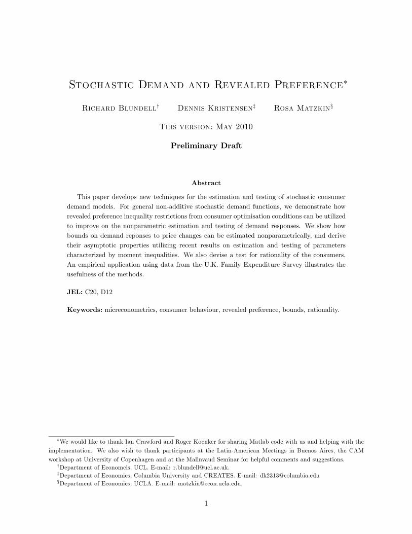
10 Empirical Application (to be completed)

In our application we apply the methodology for constructing demand bounds under revealed

preference restrictions to data from the U.K. Family Expenditure Survey. The data set contains

expenditure data and prices from UK households. We use the same sample selection as in Blundell

et al (2008) and we refer to that paper for a more detailed description. The distribution of relative

prices over the central period of the data is give in Figure 1. It shows periods of quite dense relative

prices, in the 1980s for example, and periods of sparse relative prices as in the 1970s.

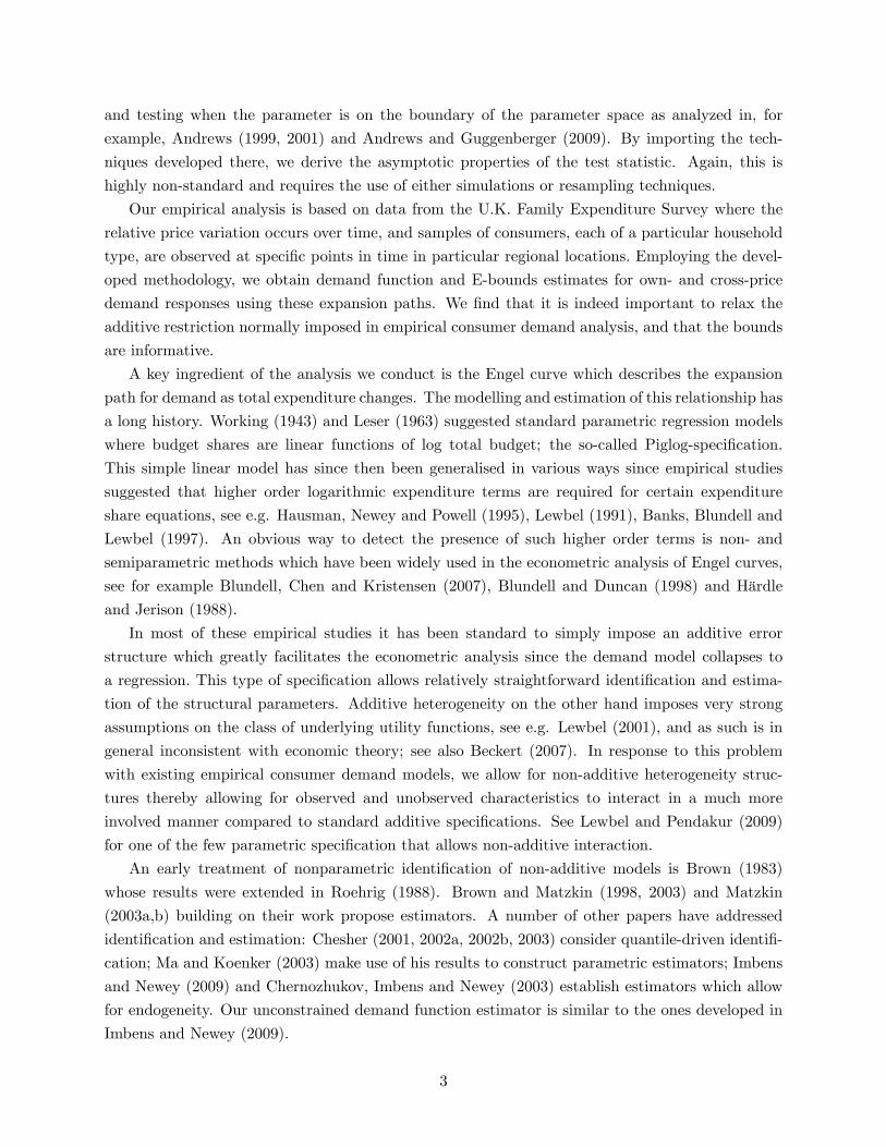
We choose food as our primary good, and then group the other goods together in this application.

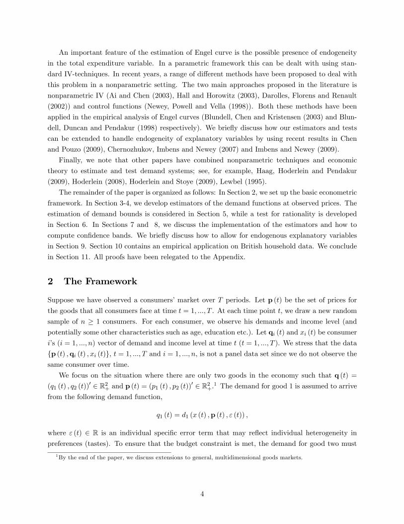
The basic distribution of the Engel curve data are described in Figures 2 and 3.

20

Figure 1: Relative prices in the UK FES: 1975 to 1999

0.92 0.94 0.96 0.98 1 1.02 1.04 1.06 1.080.75

0.8

0.85

0.9

0.95

1

1.05

1.1

1.15

1.2

1975

197619771978 1979

1980

1981

19821983 1984

198519861987

19881989

1990199119921993

1994 19951996

199719981999

Pric

e of

 ser

vice

sre

lativ

e to

 non

dura

bles

Price of foodrelative to nondurables

0.92 0.94 0.96 0.98 1 1.02 1.04 1.06 1.080.75

0.8

0.85

0.9

0.95

1

1.05

1.1

1.15

1.2

1975

197619771978 1979

1980

1981

19821983 1984

198519861987

19881989

1990199119921993

1994 19951996

199719981999

Pric

e of

 ser

vice

sre

lativ

e to

 non

dura

bles

Price of foodrelative to nondurables

Figure 2: The Engel Curve Distribution

3.5 4 4.5 5 5.5 60

0.1

0.2

0.3

0.4

0.5

0.6

Food Share

Log Expenditure

21

Figure 3: The Density of Log Consumption: UK FES

3.5 4 4.5 5 5.5 6 6.50

0.2

0.4

0.6

0.8

1

Log Expenditure

Density

kernel densitynormal density

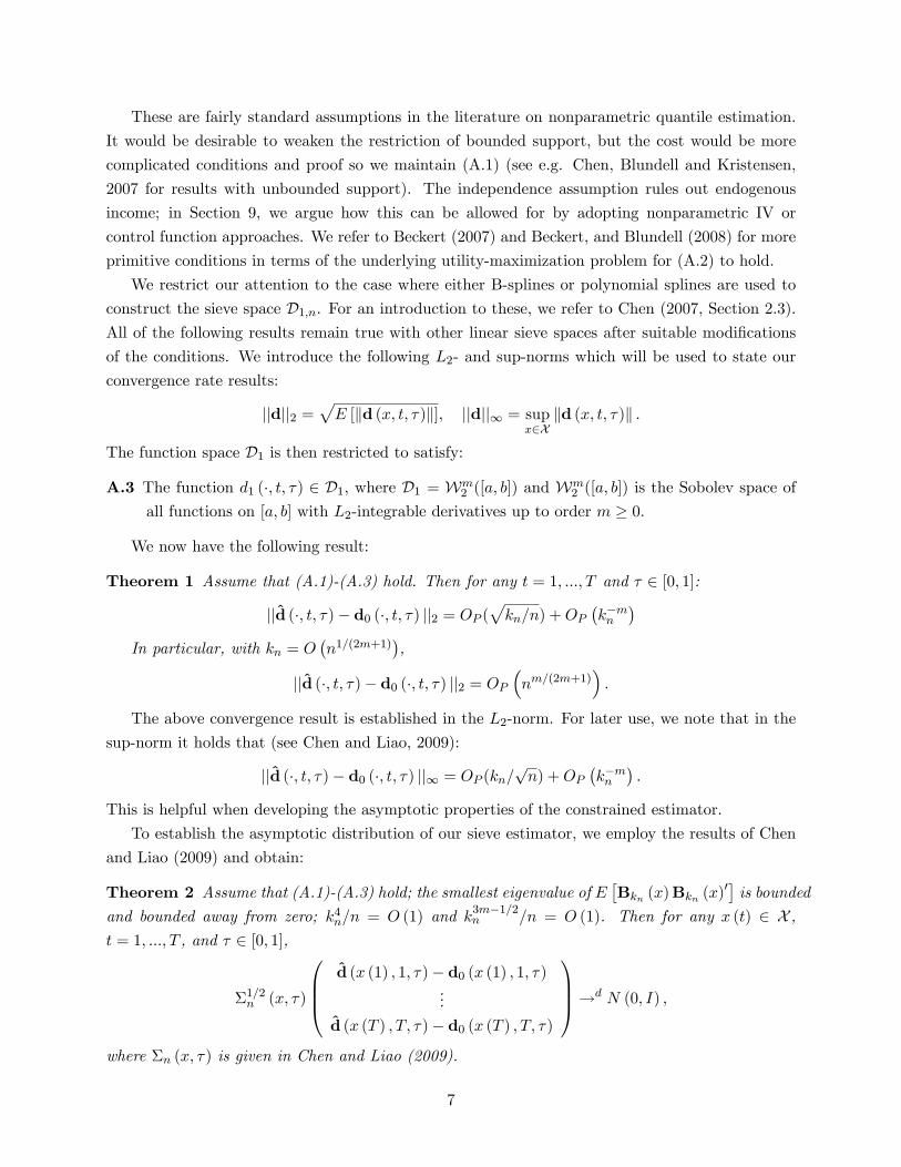
10.1 The Quantile Sieve Estimates of Expansion Paths

In the estimation, we use polynomial splines

d1;n(x; t; �) = � (t; �)0BKn(y)

0 =

qnXj=0

�j (t; �)xj +

rnXk=1

�qn+k (t; �) (x� �k (t))qn+ ; Kn = qn+ rn+1;

(20)

where qn � 1 is the order of the polynomial and �k, k = 1; :::; rn, are the knots. For a given choiceof rn, we place the knots according to the sample quantiles of xi (t), i = 1; :::; n, i.e., �k (t) was

chosen as the estimated k= (rn + 1)-th quantile of x (t) :

In the implementation of the quantile sieve estimator, a small penalization term was added to

the objective function to robustify the estimators (see Blundell, Chen and Kristensen, 2007 for a

similar approach). That is,

� (t; �) = arg min�2RjKnj

1

n

nXi=1

���q1;i (t)� �0Wi (t)

�+ �Q (�) ; � 2 [0; 1] ; (21)

where

Wi (t) =�1; xi (t) ; :::; xi (t)

q ; (x� �1 (t))qn+ ; :::; (x� �rn (t))qn+

�0;

and �Q (�) is an L1-penalty term. Here, Q (�) is the total variation of @dn;1 (x) = (@x),

Q (�) =

Z b

a

�����0@2B (x)@x2

���� dx 2 R+;while � > 0 is the penalization weight that controls the smoothness of the resulting estimator.

22

Figure 4: ��Quantile Expansion Paths for Food Shares

4 4.5 5 5.5 6 6.5 70

0.05

0.1

0.15

0.2

0.25

0.3

0.35

0.4

0.45

0.5

lnx

shar

e

τ = 0.05τ = 0.25τ = 0.50τ = 0.75τ = 0.95

4 4.5 5 5.5 6 6.5 70

0.05

0.1

0.15

0.2

0.25

0.3

0.35

0.4

0.45

0.5

lnx

shar

e

τ = 0.05τ = 0.25τ = 0.50τ = 0.75τ = 0.95

By following the arguments of Koenker, Ng and Portnoy (1994), the above estimation problem

can be formulated as a linear programming problem. The computation of the unrestricted estimator

was done using Matlab code kindly provided by Roger Koenker.

The restricted estimator is computed by solving the least-squares problem in Eq. (19). We

opted for this estimator instead of the quantile estimator proposed in Eq. (18) since numerically

we found it easier to solve the constrained least-squares problem.

In our application, we focus on the six year period 1983-1988. As in Blundell at al (2008) we

use a group of demographically homogeneous households and estimate conditional quantile spline

expansion paths using a 3rd order polynomial (qn = 3) with rn = 5 knots. The RP restrictions are

imposed at 100 x-points over the empirical support x (log total expenditure on non-durables and

services).

Each household is de�ned by a point in the distribution of log income and unobserved het-

erogeneity (x; "): For households at the median of the income (total expenditure) distribution the

unrestricted ��quantile expansion paths for food share are given in Figure 4.

10.2 Estimated Demand Bounds

The key parameter of interest in this study is the consumer response at some new relative price

p0 and income x or at some sequence of relative prices. The later de�nes the demand curve for

(x; "). The estimated (e-)bounds (support sets) using the revealed preference inequalities and our

FES data are given in Figures 5-8.

The Figures display the bounds on demand responses across the two dimensions of individual

23

Figure 5: Quantile (RP-Rest) e-Bounds on Demand (Median InC) � = :50

1 1.02 1.04 1.06 1.08 1.1 1.12 1.14 1.16 1.180

10

20

30

40

50

60Demand bounds, τ = 0.50

price, food

dem

and,

 food

heterogeneity - income and unobserved heterogeneity. For a given income we can look at demand

bounds for consumers with stronger or weaker preferences for food. Figure 5 shows the bounds on

demands at the median income for the 50th percentile (� = :5) of the unobserved taste distribution.

Notice that where the relative prices are quite dense the bounds are correspodngly narrow. Figure

6 contrasts this for a consumer at the 25% percentile of the heterogeneity distribution - a consumer

with much weaker taste for food. At all points demands are much lower and the price response

is somewhat less steep. Figure 7 considers a consumer with a strong taste for food - at the 75th

percentile of the taste distribution. Demand shifts up at all points. The bounds remain quite

narrow where the relative prices are dense. Finally, to illustrate the power of this approach, Figure

8 considers a higher income consumer but with median taste for food.

11 Conclusion

This paper has developed a nonparametric estimator of revealed-preference restricted demand

functions and their associated demand bounds for the case of nonseparable heterogeneity. The

asymptotic properties of the estimators were derived and the implementation discussed. A test for

rationality was proposed and its asymptotic properties analyzed.

24

Figure 6: Quantile (RP-Rest) e-Bounds on Demand (Median Inc) � = :25

1 1.02 1.04 1.06 1.08 1.1 1.12 1.14 1.16 1.180

10

20

30

40

50

60Demand bounds, τ = 0.25

price, food

dem

and,

 food

Figure 7: Quantile (RP-Rest) e-Bounds on Demand (Median Inc) � = :75

1 1.02 1.04 1.06 1.08 1.1 1.12 1.14 1.16 1.180

10

20

30

40

50

60Demand bounds, τ = 0.75

price, food

dem

and,

 food

25

Figure 8: Quantile (RP-Rest) e-Bounds on Demand (75% Inc)

1 1.02 1.04 1.06 1.08 1.1 1.12 1.14 1.16 1.180

10

20

30

40

50

60Demand bounds, τ = 0.50

price, food

dem

and,

 food

References

Afriat, S.N. (1973): "On a System of Inequalities in Demand Analysis: An Extension of the Classical

Method," International Economic Review 14, 460-472.

Anevski, D. and O. Hössjer (2006): "A General Asymptotic Scheme for Inference Under Order

Restrictions," Annals of Statistics 34, 1874-1930.

Andrews, D.W.K. (1997): "Estimation When a Parameter Is on a Boundary: Theory and Appli-

cations," Cowles Foundation Discussion Paper No. 1153.

Andrews, D.W.K. (1999): "Estimation When a Parameter Is on a Boundary," Econometrica 67,

1341-1383.

Andrews, D.W.K. (2001): "Testing When a Parameter Is on the Boundary of the Maintained

Hypothesis," Econometrica 69, 683-734.

Andrews, D.W.K. and P. Guggenberger (2009): "Validity of Subsampling and �Plug-in Asymptotic�

Inference for Parameters De�ned by Moment Inequalities," Econometric Theory 25, 669-709.

Andrews, D.W.K. and G. Soares (2010): "Inference for Parameters De�ned by Moment Inequalities

Using Generalized Moment Selection," forthcoming in Econometrica.

W Beckert (2007): "Speci�cation and Identi�cation of Stochastic Demand Models," Econometric

Reviews 26, 669-683.

26

Beckert, W. and R. Blundell (2008): "Heterogeneity and the nonparametric analysis of consumer

choice: conditions for invertibility," Review of Economic Studies 75, 1069-1080.

Beresteanu, A. (2006): "Nonparametric Estimation of Regression Functions under Restrictions on

Partial Derivatives," working paper, Duke University.

Birke, M. and H. Dette (2007): "Estimating a Convex Function in Nonparametric Regression,"

Scandinavian Journal of Statistics 34, 384-404.

Blundell, R., M. Browning and I. Crawford (2003): "Nonparametric Engel Curves and Revealed

Preference," Econometrica 71, 205-240.

Blundell, R., M. Browning and I. Crawford (2008): "Best Nonparametric Bounds on Demand

Responses," Econometrica 76, 1227-1262.

Blundell, R., X. Chen and D. Kristensen (2007): "Semi-Nonparametric IV Estimation of Shape-

Invariant Engel Curves," Econometrica 75, 1613-1669.

Brown, B.W. (1983): "The Identi�cation Problem in Systems Nonlinear in the Variables," Econo-

metrica, 51, 175-196.

Bugni, F. (2009): "Bootstrap Inference in Partially Identi�ed Models De�ned by Moment Inequal-

ities: Coverage of the Points of the Identi�ed Set," manuscript, Department of Economics,

Duke University.

Bugni, F. (2010): "Bootstrap Inference in Partially Identi�ed Models De�ned by Moment Inequal-

ities: Coverage of the Identi�ed Set," forthcoming in Econometrica.

Chen, X. (2007): "Large Sample Sieve Estimation of Semi-Nonparametric Models," in Handbook

of Econometrics, Vol. 6B (eds. J. Heckman and E. Leamer), 5549-5632. Amsterdam: North-

Holland.

Chen, X. and Z. Liao (2009): �On Limiting Distributions of Possibly Unbounded Functionals of

Linear Sieve M-Estimators,�Manuscript, Yale University.

Chen, X. and D. Pouzo (2007): "Estimation of Nonparametric Conditional Moment Models with

Possibly Nonsmooth Moments," Cowles Foundation Discussion Papers, No. 1650.

Chen, X. and X. Shen (1998): �Sieve Extremum Estimates for Weakly Dependent Data,�Econo-

metrica 66, 289-314.

Chernozhukov, V., I. Fernandez-Val and A. Galichon (2006): "Improving Point and Interval Esti-

mators of Monotone Functions by Rearrangement," Biometrika 96, 559�575.

Chernozhukov, V., G. Imbens and W.K. Newey (2007): "Instrumental Variable Estimation of

Nonseparable Models," Journal of Econometrics 139, Pages 4-14

27

Chernozhukov, V., H. Hong and E. Tamer (2007): "Estimation and Con�dence Regions for Para-

meter Sets in Econometric Models," Econometrica 75, 1243 - 1284.

Chesher, A. (2003): "Identi�cation in Nonseparable Models," Econometrica 71, 1405-1441.

Gallant, A. R. & Golub, G. H. (1984): "Imposing Curvature Restrictions on Flexible Functional

Forms," Journal of Econometrics 26, 295-321.

Haag, B.R., S. Hoderlein and K. Pendakur (2009): "Testing and imposing Slutsky symmetry in

nonparametric demand systems," Journal of Econometrics 153, 33-50.

Hall, P. (1992): The Bootstrap and Edgeworth Expansion. New York: Springer Verlag.

Hall, P. and J. Horowitz (2005): "Nonparametric Methods for Inference in the Presence of Instru-

mental Variables," Annals of Statistics 33, 2904-2929.

Hausman, J.A., W.K. Newey & J.L. Powell (1995): "Nonlinear Errors in Variables: Estimation of

Some Engel Curves," Journal of Econometrics 65, 205-233.

Hoderlein, S. (2008): "How Many Consumers are Rational?" Manuscript, Dep. of Economics,

Brown University.

Hoderlein, S. and J. Stoye (2009) "Revealed Preferences in a Heterogeneous Population," Manu-

script, Dep. of Economics, Brown University.

Imbens, G. and W.K. Newey (2009): "Identi�cation and Estimation of Triangular Simultaneous

Equations Models without Additivity," Econometrica 77, 1481-1512.

Kiefer, J. (1982): "Optimum Rates for Non-parametric Density and Regression Estimates under

Order Restrictions," in Statistics and Probability: Essays in Honor of C. R. Rao (eds. G.

Kallianpur , P.R. Krishnaiah & J.K. Ghosh), 419-428. Amsterdam: North-Holland.

Kim, M.-O. (2006) Quantile Regression with Shape-Constrained Varying Coe¢ cients. Sankhya 68,

369-391.

Klepper, S. and E.E. Learner (1984): "Consistent Sets of Estimates for Regressions with Errors in

All Variables," Econometrica 52, 163-184.

Koenker, R. and G. Bassett, Jr. (1978): "Regression Quantiles," Econometrica 46, 33-50.

Koenker, R. and P. Ng (2005): "Inequality Constrained Quantile Regression," Sankhya 67, 418-440.

Koenker, R., P. Ng and S. Portnoy (1994): "Quantile smoothing splines," Biometrika 81, 673-680.

Leser, C. E. V. (1963) Forms of Engel Functions. Econometrica, 31, 694-703.

Lewbel, A. (1991): "The Rank of Demand Systems: Theory and Nonparametric Estimation,"

Econometrica, 59, 711-730.

28

Lewbel, A. (1995): "Consistent nonparametric hypothesis tests with an application to Slutsky

symmetry," Journal of Econometrics 67, 379-401.

Lewbel, A. (2001): "Demand Systems With and Without Errors," American Economic Review 91,

611-618.

Lewbel, A. and K. Pendakur (2009): "Tricks With Hicks: The EASI Demand System," American

Economic Review 99, 827-863.

Mammen, E. (1991): "Estimating a Smooth Monotone Regression Function," Annals of Statistics

19, 724-740.

Mammen, E., J.S. Marron, B.A. Turlach and M.P. Wand (2001): "A General Projection Framework

for Constrained Smoothing," Statistical Science 16, 232�248.

Mammen, E. and C. Thomas-Agnan (1999): "Smoothing Splines and Shape Restrictions," Scandi-

navian Journal of Statistics 26, 239-252.

Matzkin, R.L. (2003): "Nonparametric Estimation of Nonadditive Random Functions," Economet-

rica, 71, 1339-1375.

Matzkin, R.L. (2005): "Identi�cation in Nonparametric Simultaneous Equations," Econometrica

76, 945 - 978

Mukerjee, H. (1988): "Monotone Nonparametric Regression," Annals of Statistics 16, 741-750.

Newey, W.K. & J. Powell (2003): "Instrumental Variables Estimation for Nonparametric Models,"

Econometrica, 71, 1565-1578.

Roehrig, C.S. (1988) Conditions for Identi�cation in Nonparametric and Parametric Models. Econo-

metrica, 56, 433-447.

Van de Geer, S. (2000): Empirical Processes in M-estimation. Cambridge University Press.

Van der Vaart, A. and J. Wellner (1996): Weak Convergence and Empirical Processes: With

Applications to Statistics. Springer-Verlag, New York.

Working, H. (1943): "Statistical Laws of Family Expenditure," Journal of the American Statistical

Association, 38, 43-56.

Wright, F.T. (1981): "The Asymptotic Behavior of Monotone Regression Estimates," Annals of

Statististics 9, 443-448.

Wright, F.T. (1984): "The Asymptotic Behavior of Monotone Percentile Regression Estimates,"

Canadian Journal of Statistics 12, 229-236.

Yatchew, A. and Bos, L. (1997): "Nonparametric Regression and Testing in Economic Models,"

Journal of Quantitative Economics 13, 81{131.

29

A Proofs of Section 2 and 3

Proof of Theorem 1. We suppress the dependence on t since it is kept �xed in the following.

Write the �rst demand equation as a quantile regression,

q1 = d1 (x; �) + e (�) ; (22)

where e is de�ned as the generalized residual, e (�) := d1 (x; ") � d1 (x; �). This formulation ofthe model for corresponds to the quantile regression considered in Chen (2007, Section 3.2.2). We

then wish to verify the conditions stated there. First, we show that the distribution of e (�) jx isdescribed by a density ft;� (ejx) that satis�es

0 < infx2X

f� (ejx) � supx2X

f� (ejx) <1; (23)

supx2X

jf� (ejx)� f� (0jx)j ! 0; jej ! 0: (24)

To see this, we �rst note that due to the independence between x and ", the invertibility and

di¤erentiability of " 7! d1 (x; "), and that " � U [0; 1],

f� (ejx) = I�0 � d�11 (x; e� d (x; �)) � 1

����@d�11 (x; e� d1 (x; �))@e

���� :From this expression it is easily seen that Eq. (23) holds since d1 (x; t; ") and its derivative w.r.t.

" are continuous in x and X is compact. Eq. (24) clearly holds pointwise due to the continuity of

" 7! d1 (x; "). This can be extended to uniform convergence since supx2X ;e2[0;1] f� (ejx) <1.Combining the above results with the arguments given in in the Proof of Chen (2007, Proposition

3.4), we now conclude that Chen (2007, Theorem 3.2) applies such that

jjd (�; t; �)� d0 (�; t; �) jj2 = OP (max f�n; k�nd1;0 (�; t; �)� d1 (�; t; �)kg)

where

�n = inf�2(0;1)

�1

pn�2

Z �

b�2

qH[] (w;Fn; k�k)dw � const.

�;

and �nd1;0 is an element in D1;n. Here, H[] (w;Fn (�) ; k�k2) = log�N[] (w;Fn (�) ; k�k2)

�with

N[] (w;Fn (�) ; k�k2) denoting the so-called L2-covering numbers with bracketing of the functionclass Fn (�), see Van der Vaart and Wellner (1996) and van de Geer (2000) for the precise de�n-itions. To complete the proof, we appeal to Chen and Shen (1998, p. 311) to obtain that in the

case of splines �n = O(pkn=n) and k�nd1;0 (�; t; �)� d1 (�; t; �)k = O (k�mn ).

Proof of Theorem 2. The result for T = 1 follows directly from Chen and Liao (2009) under

their Conditions 6.1-6.2, which we now verify. First, Condition 6.1 is shown to hold in the Proof

of Theorem 1. Second, Condition 6.2 holds since

jf� (e1jx)� f� (e2jx)j � C����@d�11 (x; e1 � d1 (x; �))

@e� @d

�11 (x; e2 � d1 (x; �))

@e

���� � C je1 � e2j ;30

where we have used that d1 is continuously di¤erentiable.

The extension to T > 1, follows by de�ning the functional

�� (d) = �01d0 (x (1) ; 1; �) + :::�

0Td0 (x (T ) ; T; �) ;

for any given � = (�1; :::; �T ). We can proceed as in Chen and Liao (2009) to show asymptotic

normality of ��(d)��� (d). Since this holds for any �, the claimed result now follows by the

Cramer-Wold device.

Proof of Theorem 3. Let rn = kn=pn + k�mn denote the uniform rate of the unrestricted

estimator, and let x0 (t) be a given income expansion path generated from d. We �rst note that

the expansion path based on the unconstrained demand function satis�es

x (T � 1) := p (T � 1)0 d (x (T ) ; t; �) = x0 (T � 1) +OP (rn) :

By recursion, we easily extend this to maxt=1;:::;T jx (t)� x0 (t)j = OP (rn). Thus,

x (t)� p (t)0 d (x (s) ; s; �) = fx (t)� x0 (t)g+ p (t)0nd0 (x0 (s) ; s; �)� d (x (s) ; s; �)

o+x0 (t)� p (t)0 d0 (x0 (s) ; s; �)

= OP (rn) :

Thus, as rn ! 0, x (t) � p (t)0 d (x (s) ; s; �) � � with probability approaching one (w.p.a.1) as

rn ! 0. This proves that d 2 DTC;n (�) w.p.a.1 such that d�C = d w.p.a.1 as rn ! 0. Since the

restricted and unrestricted estimators are asymptotically equivalent, they share convergence rates

and asymptotic distributions.

B Proof of Theorem 4

We here prove a more general version of Theorem 4 since we believe this has independent interest.

In particular, the general result takes as input any set of demand function estimators and derive the

asymptotic properties of the corresponding bounds. The result is stated in such a fashion that it

allows for both fully parametric, semi- and nonparametric �rst-step estimators. Let in the following

d (x; t) = (d1 (x; t) ; :::; dL (x; t))0 be any given set of demand function estimators for L � 2 goods.

We then assume that the following conditions are met:

C.1 x (t) 7! d0 (x (t) ; t) is montonically increasing.

C.2 The matrix P = [p (1) ; � � � ;p (T )]0 2 RT�L+ has rank L.

C.3 For some sequence rn !1, and for any vector x = (x (1) ; :::; x (T )) 2 RT+:

(i) maxt=1;:::;T d (x (t) ; t)� d0 (x (t) ; t) = OP �1=prn�.

31

(ii)

prn

0BB@d (x (1) ; 1)� d0 ((1) ; 1)

...

d (x (T ) ; T )� d0 (x (T ) ; T )

1CCA!d N (0;� (x)) ;

where � (x) 2 RLT�LT is the joint asymptotic variance of the sequence of demand

function estimators.

We then show the following result which includes our sieve estimator as a special case:

Theorem 6 Assume that (C.1)-(C.3) hold. Then the conclusions of Theorem 4 hold for the generaldemand estimator in (C.3).

To show this result, we �rst de�ne b and b by

bt = p (t)0 d0(x (t) ; t); bt = p (t)

0 d(x (t) ; t); t = 1; :::; T;

where

p00d0(t; x (t)) = p00d0(t; x (t)) = x0; t = 1; :::; T;

while A = P where P is given in Assumption C.2. The support set now takes the form considered

in Appendix C, and we verify Assumptions 1�2 and 4 of Theorem 10 stated there. It is easily seen

that Assumptions 1-2 hold, so we only have to verify Assumptions 4: We have

prn

�b� b

�= �P

prn

�D �D

�;

where D = (d(1; x (1))0; :::; d(T; x (T ))0)0 2 RLT , D = (d0(1; x (1))0; :::;d0(T; x (T ))0)0 2 RLT and

�P =

2666664p (1)0 0 � � � 0

0 p (2)0...

.... . . 0

0 � � � 0 p (T )0

3777775 2 RT�LT :

We write

D �D =nD � ~D

o+�~D �D

�;

where ~D = (d(1; x (1)); :::; d(T; x (T )))0. We then wish to derive the joint asymptotic distribution

of�D � ~D; ~D �D

�. We �rst derive the asymptotics of x (t) which is characterized by

0 = p00d(t; x (t))� x0

= p00d (t; x (t))� x0 + p00@d (t; x)

@x

�����x=x(t)

(x (t)� x (t))

= p00d (t; x (t))� x0 + p00

(@d (t; x)

@x

����x=x(t)

+ oP (1)

)(x (t)� x (t)) :

32

Thus, x = (x (1) ; :::; x (T ))0 satis�es

prn (x� x) = Q�10 �P0

prn

�~D �D

�+ oP (1) ;

where

�P0 =

2666664p00 0 � � � 0

0 p00...

.... . . 0

0 � � � 0 p00

3777775 2 RT�LT ; Q0 =

2666664p00

@d(x(1);1)@x(1) 0 � � � 0

0 p00@d(x(2);2)@x(2)

......

. . . 0

0 � � � 0 p00@d(x(T );T )@x(T )

3777775 2 RT�T :

Next, use this result to conclude that

prn

�d� ~d

�=

�@D

@x+ oP (1)

�prn (x� x) =

@D

@xQ�10

�P0prn

�~D �D

�+ oP (1) ;

where

@D

@x=

2666664@d(x(1);1)@x(1) 0 � � � 0

0 @d(x(2);2)@x(2)

......

. . . 0

0 � � � 0 @d(x(T );T )@x(T )

3777775 2 RLT�T :In total,

prn

D � ~D~D �D

!=

prn

�~D �D

�+ oP (1) ;

with

=

@d@xQ

�10�P0

ILT

!2 R2LT�LT : (25)

In conclusion,

prn

�b� b

�= �P (ILT ; ILT )

prn

D � ~D~D �D

!= �P (ILT ; ILT )

prn

�~D �D

�+ oP (1) ;

which is OP (1) under C.3(i) while under C.3(ii),

prn

�b� b

�!d N

�0; �P (ILT ; ILT )� (x)

0 (ILT ; ILT )0 �P0�:

C Proof of Theorem 5

As with Theorem 4, we here prove a more general version of the theorem that takes as input any

estimate of the demand system. As before, let d (x; t) = (d1 (x; t) ; :::; dL (x; t))0 be any given set of

demand function estimators for L � 2 goods, and let q (p0; x0) be the implied demands computedas in eqs. (10)-(11). We then show that Theorem 5 holds under the general assumptions C.1-C.3

stated in the previous section.

33

Theorem 7 Assume that (C.1)-(C.3) hold, and that Wn !P W > 0. Then the conclusions of

Theorem 5 hold for the general demand estimator in (C.3).

To prove this result, de�ne `n(q) = rnMDn(qjp0; x0) as the normalized version of the statistic,and let q be the unrestricted estimator, q = argminq2RTL+ `n(q). Clearly, q = q (p0; x0) and

`n(q) = 0. Also de�ne the restricted estimator q0by q

0= argminq2S `n(q) such that `n(q0) =

rnMD�n(p0; x0). Thus, our test can be written as

rnMD�n(p0; x0) =

n`n(q0)� `n(q0)

o�n`n(q)� `n(q0)

o; (26)

where q0= q

0(p0; x0) is given in Eq. (13). For convenience, let Z (x0;p0) = rn(q0 � d (x0;p0))

denote the normalized estimator such that Z (x0;p0) � N (0;� (x0;p0)) is its limit, Zn (x0;p0)!d

Z (x0;p0), c.f. (C.3.ii). In the following, we suppress all dependence on (x0;p0) since these are

kept �xed.

We �rst note that the second term in Eq. (26) follows a standard distribution since the criterion

function is smooth and q0is situated in the interior of RTL+ : The �rst and second order derivatives

are given by@`n(q)

@q= 2Wnrn(q� q (p0; x0));

@2`n(q)

@q@q0= 2rnWn;

and the third derivative being zero. Thus, by a third order Taylor expansion

`n(q0)� `n(q) =@`n(q)

@q(q0� q) + 1

2(q� q

0)0@2`n(q)

@q@q0(q� q

0) (27)

=prn(q (p0; x0)� q0)

0Wnprn(q (p0; x0)� q0)

= Z 0nWnZn:

The �rst term in Eq. (26) requires some more work since q0will be on the boundary of the

constrained set S as de�ned in Eq. (12). In order to deal with this, we employ the general results ofAndrews (2001) [A01]. Using his notation, the parameter of interest is � = q 2 RTL, the parameterspace is given by � = S and the objective function is given by `T (�) = `n(q) (A01 uses T for

sample size). A01�s norming matrix Bn is chosen as Bn =prn. We now verify Assumptions 1, 2 2

�,

3�, 5� and 6 in A01 for the constrained estimator such that we can appeal to his Theorem 1.

Assumptions 2 2�: We �rst note that S � q

0is a union of linear inequality constraints. Thus

Assumption 2 2�(a) holds with S+ = S \ B(q

0; �) for some (small) � > 0. Assumption 2 2

�(b) and

2 2�(c) clearly hold since `n(q) is three times di¤erentiable with B�2n @2`n(q)=(@q@q

0) = 2Wn !P

2W�1 > 0.

Assumptions 3 �: By (C.2.ii),

B�1n@`n(q0)

@q= 2Wn

prn�q� q (p0; x0)

�= 2WnZn !d 2W�1Z;

while B�2n @2`n(q)=(@q@q0)!P 2W�1 > 0 by (C.3).

34

Assumptions 5 � and 6: We wish to �nd a cone that is locally equal to S� q0. To this end, we

wish to write S on the form

S =�qjV �t (q)� V �s (q) � ��t (q)p (t)

0 (q (s)� q (t)); s; t = 1; :::; T;

for some functions V � : RLT+ 7! RT+ and �� : RLT+ 7! RT+ that takes any set of demands, q =�q (1) ; :::;q (T )

�and maps it into an associated set of unique utility levels and marginal utilities. For

q 2 S, the mapping can be constructed by, for example, Varian/Arifat�s algorithm. Alternatively,we may de�ne the two mappings as

(V (q); �(q)) = arg minV;�2RT

V 0V + �0�

s.t. Vt � Vs � �tp (t)0 (q (s)� q (t)) ; �t � 1; Vt > 0; t = 1; :::; T:

This convex optimization problem has a unique solution for any given value of q 2 S. However,this mapping is only de�ned for q 2 S - not outside of the set. And we need the mapping to bewell-de�ned and di¤erentiable in a small neighbourhood of q

0. If q

0lies on the boundary of S, this

implies that we need to extend the mapping to also be well-de�ned outside of S. For any q and(V; �) satisfying with

q� q� < � and (V; �)� (V (q�); �(q�)) < �, for some small � > 0, de�nee(q; V; �) as

e(q; V; �) = argmine�0

e2

s.t. Vt � Vs + e � �tp (t)0 (q (s)� q (t)) ; t = 1; :::; T:

This is a well-de�ned function, which is continuously di¤erentiable in a small neighbourhood of

(q�; V (q�); �(q�)). For any q with q� q� < �, we now rede�ne (V (q); �(q)) as

(V (q); �(q)) = argminV;�

V 0V + �0�

s.t. Vt � Vs + e(q; V; �) � �tp (t)0 (q (s)� q (t)) ; �t � 1; Vt > 0; t = 1; :::; T:

The solution mapping (V (q); �(q)) is di¤erentiable for q with q� q� < �, and we can restrict

our attention to this set since under the null, q� ! q�.With B(q) de�ned in Section 7, we can then

write the constrained set as S = fqjB(q) � 0g, and employ Andrews (1997, Lemma 2) to obtainthat the cone � is given as in Eq. (15).

It now follows by A01, (proof of) Theorem 1, that

`n(q0)� `n(q) = Z0nWZn � inf

�2�(�� Zn)0Wn (�� Zn) + oP (1) : (28)

Substituting Eqs. (27) and (28) back into Eq. (26) yields the desired result:

MD�n (x0) = inf�2�

(�� Zn)0 W + oP (1)!d inf�2�

(�� Z)0W�1 (�� Z) :

35

D Auxiliary Results

We here state a general result for a family of set estimators involving linear constraints. These

should have independent interest outside of demand bounds estimation. In particular, this seems

to be the �rst general treatment of linear two-step set estimators. We consider a compact and

convex parameter space � � Rd and de�ne the set of identi�ed parameters by

�I = f� 2 �jA� � bg ;

for some known function � : � 7! Rq and some unknown matrix A 2 Rp�q and unknown vectorb 2 Rp. Since A and b are unknown, we cannot compute �I , but suppose we are given preliminaryestimators, A = An 2 Rp�q and b = bn 2 Rp for some sample of size n � 1. A natural estimator of�I is then the following plug-in one,

�I =n� 2 �jA� � b

o:

However, in some situations, a di¤erent estimator has to be used to ensure that the estimator is

consistent and in order to construct con�dence sets, c.f. Section 3.

We note that by de�ning

m (�) = A� � b; m (�) = A� � b;

we can express �I and �I in terms of a set of moment inequalities: �I = f� 2 �jm (�) � 0g and�I = f� 2 �jm (�) � 0g.

As already demonstrated in Section 7, the demand bound estimator �ts into this framework.

Some other problems are:

Example 8 (OLS with Errors-in-Variables) Consider the regression model

Y = �0 + �01X + ";

where we only have contaminated observations of X 2 Rd,

Z = X + u:

Here, ut are the errors-in-variables. Assuming that u and X are independent with E [u] = 0 and

E [uu0] = D, we obtain by following e.g. Klepper and Leamer (1984) that �1 satis�es

r0b1 � r0�1 � Var (Y ) ;

where

b1 = Var (Z)�1Cov (Z; Y ) 2 Rd; r = Cov (Z; Y ) 2 Rd:

Here,

A = [r;�r]0 2 R2�d; b =�Var (Y ) ;�r0b1

�0 2 R2:36

Example 9 (Regression with Interval-Censored Outcomes) Consider the regression model

Y = �0X + ";

where X 2 fx1; :::; xLg is discrete and we don�t observe Y but only Ymin and Ymax where Y 2[Ymin; Ymax]. Then

E [YminjX = xi] � �0xi � E [YmaxjX = xi] ; i = 1; :::; L:

Here,

A =�x01; ::::; x

0L

�2 RL�d; b = (E [YminjX = x1] ; :::; E [YminjX = xL])

0 2 RL:

We derive the asymptotic properties of �I and construct con�dence sets for �I by utilizing the

general set of results found in Chernozukhov, Tamer and Hong (2007) [CHT07]. We will do so

under the following high-level assumptions:

Assumption 1 The parameter space � � Rd is compact and convex.

Assumption 2 The matrix A =�a01; :::; a

0p

�0 2 Rp�d, ai 2 Rd, has rank p.Assumption 3 The set

��"I = f� 2 �I jai� � bi � "; i = 1; :::; pg � �I

has a non-empty interior for some (su¢ ciently small) " > 0.

Assumption 4 For some sequence rn !1:

(i) jjA�Ajj = OP�1=prn�and jjb� bjj = OP

�1=prn�.

(ii)

prn

vec

�A�� vec (A)

b� b

!!d N

0;

AA Ab

bA bb

!!;

where V 2 Rp(d+1)�p(d+1) is the joint asymptotic variance.

Depending on whether Assumption 3 holds or not, we will use two di¤erent estimators of �I .

These can both be written on the form

�I(c) =

(� 2 �j sup

�2�Ijjm (�) jj2+ � c=rn

);

for some sequence c = cn � 0, and where jjxjj2+ = kmax fx; 0gk2. If Assumption 3 does not hold,

then int�I = ?, and we need to choose � / log (n) to obtain consistency. If it does hold, we maychoose � = 0 such that �I = �I (0) =

n� 2 �jA� � b

o.

In order to do inference, we wish to choose a (possibly data dependent) sequence � such that

P (�I � �I(�))! 1� �;

for some given con�dence level 1��. Here, we need to choose � > 0 to obtain the correct coverage,even if �I(0) is consistent.

37

Theorem 10 Assume that Assumptions 1-2 and 4(i) hold.

1. If Assumption 3 does not hold, we choose c / log (n), and obtain:

dH(�I (�) ;�I) = OP (plog (n) =rn):

2. If Assumption 3 does hold, we choose c = 0 and obtain:

dH(�I (0) ;�I) = OP (p1=rn):

3. If additionally Assumption 4(ii) hold then

sup�2�I

rnQn (�)!d Q := sup�2�I

kZ (�) + � (�)k2+ ;

where � 7! Z (�) is a zero-mean Gaussian process with covariance matrix

� (�1; �2) =

�01 Ip Op�p

Op�pd �Ip

! AA Ab

bA bb

! �2 Ip Opd�p

Op�p �Ip

!;

while � (�) =��1 (�) ; :::; �p (�)

�is given by

�i (�) =

(�1; ai� < bi

0; ai� = bi; i = 1; :::; p:

Let consistent estimator c1�� of the (1� �)th quantile of Q. We then have

P (�I � �I(�))! 1� �;

where � is given by

Assumption 3 does not hold : � = c1�� +OP (log (n)) ;

Assumption 3 does hold : � = c1��:

Proof. We verify conditions C.1-C.5 in CHT07 with Qn (�) = jjm (�) jj2+, m (�) = A� � b, andQ (�) = jjm (�) jj2+, m (�) = A� � b. This will yield the stated results.

Condition C.1: Given the de�nitions of Qn (�) and Q (�), this holds with an = rn and bn =prn

as an immediate consequence of Assumption 1 and Assumption 3(i).

Condition C.2: We show that this holds with = 1. Consider any � 2 �n�I : Let �� =argmin�02�I jj�� �

0jj be the unique point in �I which has minimum distance to �. Let �� = �� ��

be the di¤erence such that k��k = � (�;�I). We can decompose the rows of (A; b) into binding andnon-binding constraints respectively of ��. We write A =

�a01; :::; a

0p

�0, where ai 2 Rd is an individualrow of A. Let

�A(1); b(1)

�and

�A(2); b(2)

�, with A(1) =

ha(1)01 ; :::; a

(1)0p1

i0and b(1) = (b

(1)1 ; :::; b

(1)p1 )

0,

denote the set of rows which contain the binding and non-binding constraints respectively. That

38

is, m(1) (��) := A(1)�� � b(1) = 0 while m(2) (��) := A(2)�� � b(2) < 0. Let �min be the minimum

eigenvalue of AA0. Due to Assumption 1, �min > 0 and we have

�min k��k � A(1)�� � max

i=1;:::;p1ja(1)i �

�j:

Thus, there exists at least one i0 2 f1; :::; p1g such that either a(1)i0 �� � ��min k��k or �min k��k �

a(1)i0��. We then obtain

km (�)k2+ =

pXi=1

jai� � bij2+ ����a(1)i0 � � b(1)i� ���2+ = ���a(1)i� (�� + ��)� b(1)i� ���2+

=���a(1)i� �����2

+� �2min k��k

2 = �2min�2 (�;�I)

This establishes that Q (�) = km (�)k2+ � �2min�2 (�;�I). Following the same steps as in CHT07�sProof of Theorem 4.2(Step 1) this veri�es (C.2).

Condition C.3: Assume that Assumption 3 holds. Consider for any (small) " > 0, the con-

traction ��"I de�ned in Assumption 3. Note that we here do not use the same contraction as the

one considered in CHT07, Section 4.2. We then wish to verify their (C.3) with �n = ��"nI where

"n = OP�1=pan�. For any � 2 �n,

nQn (�) = n km (�)�m (�) +m (�)k2+

�pXi=1

j�pnmi (�)�m (�)

+pnm (�) j2+

=

pXi=1

jOP (1) +pnm (�) j2+

�pXi=1

jOP (1) +pan"nj2+

= 0:

Next, observe that, due to ��"I � �I with both being compact,

dH(��"I ;�I) = sup

�2�I�(�;��"I ) = sup

�2�Iinf

��2��"Ik�� � �k =

��� � �� ;for some �� 2 �I and ��� 2 ��"I . These optimizers must satisfy �� 2 @�I and ��

� 2 @��"I ; in particular,there exists i 2 f1; :::; pg such that mi(��

�) = 0. Thus, ��� � �� � �max ��mi(���)�mi(��)

�� = �max ��mi(���)�� � �max";

where �max is the maximum eigenvalue of AA0.

Condition C.4-C.5: We here follow the same arguments as in CHT07, Proof of Theorem 4.2

(Step 2-3), and verify their high-level conditions in M.2 for our speci�c choice of m. De�ne

�I = f� 2 �jai� = bi; i 2 T , ai� < bi; i 2 Icg ;

39

for any subindex I � f1; :::; pg with Ic = f1; :::; pg nI, which is convex as the intersection of twoconvex sets. Also, de�ne

V�n;I =n(�; �) 2 �I �B (0; �)j� =

pan (�I � �)

o;

V�1;I =n(�; �) 2 �I �B (0; �)j� =

pan0 (�I � �) for some n0 � 1

o:

Since �I � B (0; �) is convex, it follows that V�n;I " V�1;I montonically in the set-theoretic sense.Since V�n;I ;V�1;I � �I � B (0; �) where �I � B (0; �) is compact, this in turn implies convergencein the Hausdor¤ distance.

Re. convergence of m: We have

pan (m (�)�m (�)) =

pan(A�A)� �

pan(b� b)

=��0 Ip

�panvec(A�A)�

pan(b� b)

=

�0 Ip Op�p

Op�pd �Ip

!pan

vec(A�A)b� b

!:

Under Assumption 2(i), the last expression is OP (1) while under Assumption 2(ii) it converges

towards N (0;� (�; �)). This shows pointwise weak convergence, while the following inequality

demonstrates that � 7! pan fm (�)�m (�)g is stochastically equicontinuous:

jjpan fm (�1)�m (�1)g �pan fm (�2)�m (�2)g jj = jjpan

�A�A

�(�1 � �2) jj

� pan(A�A) k�1 � �2k

= OP (1)� k�1 � �2k :

In total, the stochastic process � 7! pan fm (�)�m (�)g weakly converges on the compact set �

towards a zero-mean Gaussian process Z (�) with Cov(Z (�1) ; Z (�2)) = � (�1; �2), c.f. Van der

Vaart and Wellner (2000, Example 1.5.10). We also note that r�m (�) = A is well-de�ned. In

conclusion,

`n (�; �) = rnQn (� + �=prn)!d `1 (�; �) = kZ (�) +A�k2+ :

In particular,

sup�2�I

rnQn (�) = sup(�;�)2V01

`n (�; �)!d �Q = sup�2�I

kZ (�) + � (�)k2+ :

40