stochastic model of template-directed elongation processes
TRANSCRIPT
1
Stochastic model of template-directed elongation processes in biology
Authors:
Maria J. Schilstra1,*
Chrystopher L. Nehaniv1,2
1 Biocomputation Research Group, Science & Technology Research Institute, and
2 Adaptive Systems Research
Group, School of Computer Science. University of Hertfordshire, College Lane, Hatfield AL10 9AB, UK
* Corresponding author:
Maria J. Schilstra
Biocomputation Research Group, STRI
University of Hertfordshire
College Lane
Hatfield AL10 9AB, UK
Email [email protected]
Tel +44 (0)1707 281376
Fax +44 (0)1707 284185
Summary
We present a novel modular, stochastic model for biological template-based linear chain elongation processes.
In this model, elongation complexes (ECs; DNA polymerase, RNA polymerase, or ribosomes associated with
nascent chains) that span a finite number of template units step along the template, one after another, with
semaphore constructs preventing overtaking. The central elongation module is readily extended with modules
that represent initiation and termination processes. The model was used to explore the effect of EC span on
motor velocity and dispersion, and the effect of initiation activator and repressor binding kinetics on the overall
elongation dynamics. The results demonstrate that 1) motors that move smoothly are able to travel at a greater
velocity and closer together than motors that move more erratically, and 2) the rate at which completed chains
are released is proportional to the occupancy or vacancy of activator or repressor binding sites only when
initiation or activator/repressor dissociation is slow in comparison with elongation.
Keywords
Replication, transcription, translation, initiation, elongation, termination, template-directed, Petri-net,
semaphore, stochastic, congestion, kinetics
2
Introduction
Replication, transcription, and translation are template-directed processes in which linear DNA, RNA, or
polypeptide (protein) chains are synthesized on the basis of the information stored in existing DNA (for
replication and transcription) or RNA (for translation). All three processes occur in three major stages: initiation,
elongation, and termination. During initiation, a polymerase, a molecular motor that catalyzes the
polymerization, is recruited to the initiation site on the template, and performs the first step in the synthesis of
new polymer chains. Each process requires its own kind of polymerase: DNA polymerase for replication, RNA
polymerase for transcription, and ribosomes for translation. Polymerases use some of the energy that is liberated
upon addition of a new unit to the nascent chain to move unidirectionally along the template.
Initiation may involve the binding of additional proteins called initiation factors (IFs) to specific sites in the
vicinity of the initiation site. There are many types of IFs, with different affinities for their specific binding sites
on the various templates, and different effects on initiation. Some have a stimulatory effect, increasing the
initiation rate; others act as repressors that slow down or block the initiation process.
In the elongation phase, the polymerase moves along the template, adding new units one by one to the nascent
chain. A polymerase-nascent chain complex that is moving along the template is called an elongation complex
(EC). Each polymerase step consists of (at least) two discernible sub-steps. The elongation reaction, in which a
new unit is attached to the end of the chain, is a multistep process that may take milliseconds to complete,
whereas the step that follows, translocation (the actual movement of the EC to the next unit on the template) is
over much more quickly. As a result, the EC appears to dwell for a finite amount of time in a particular position,
and then, almost instantaneously, moves forward to the next position. ECs (i.e. the polymerase-nascent chain
residing somewhere on the template) tend to be very stable, with lifetimes that may be measured in hours.
However, when an EC reaches a stop site --a specific nucleotide sequence-- the production process enters the
termination stage, in which the EC sheds the completed chain and the polymerase dissociates from the template.
Termination may require the help of proteins called termination factors, but in some cases the polymerase has
such a weak affinity for the stop site that the complex dissociates rapidly without further assistance (see e.g.
Lodish, 2004).
As IFs or IF complexes have finite affinities for their binding sites on the template, it is often assumed that the
level of activation or repression, and consequently the replication, transcription, or translation rates themselves,
are proportional to the average occupancy level (fractional saturation) of these sites (see e.g. Ackers, 1982,

3
Alon, 2006, Shea, 1985). Dynamic models based on these assumptions do not take into account that 1) IF-
template complexes have a finite lifetime, 2) polymerase recruitment and assembly1 takes time, and 3) can only
occur at vacant initiation sites; 4) ECs span several nucleotides, and 5) cannot overtake each other.
A much more sophisticated approach to the modelling of mRNA-directed protein synthesis was presented in the
late 1960s (MacDonald, 1968, MacDonald, 1969). This mean-field approach takes into consideration points 3,
4, and 5 above, and formed the basis for several in-depth analyses of template-directed processes (see e.g. Garai,
2009, Heinrich, 1980, Zouridis, 2007, and references therein).
Here, we present a discrete, stochastic model of biological linear template-directed processes that is capable of
taking into account all five conditions above. The basic model introduced here is in some respects less
comprehensive than some of the earlier models, but is easily extended to include more detail. Because of the
addition of semaphores (Dijkstra, 2002) to the basic particle-hopping scheme that describes the elongation
process, the model can be implemented quite straightforwardly in, for example, multi-purpose stochastic Petri-
net simulators, without the need for model-specific “hard-wiring” of conditional statements in software code.
We demonstrate the use of this model in the exploration of stochastic phenomena such as noise distribution and
dynamic effects that are beyond the reach of mean-field and other deterministic models.
Model
The model, shown in Figure 1, is depicted as a Petri net (Petri, 1962). The Petri net notation is eminently
suitable for representing biochemical reaction systems, as it emphasizes the discrete nature of molecular
interactions, and draws attention to the structure of, and dependencies within interaction networks. If the rules of
chemical kinetics are used to characterize dynamic tendencies within the network, the Petri net notation is
equivalent to the standard chemical reaction notation, and can be used to automatically derive the stoichiometry
and rate equations that are used to compute the temporal development of chemical reaction systems (see, e.g.,
Schilstra, 2009, Wilkinson, 2006).
The Petri net terminology is somewhat idiosyncratic, and fairly different from the standard vocabulary used to
describe chemical reaction systems. In brief, a Petri net is a bipartite directed graph, in which nodes usually
indicated as places are connected to nodes that are generally called transitions. Places that are connected to a
transition via input arcs, arcs pointing toward the transition, are referred to as the transition’s input places; arcs
1 Polymerases consist of several subunits that assemble at or near the initiation site to form a fully functional motor. After dissociation from
the termination site, the motor disassembles into its constituent subunits.
4
pointing toward places are output arcs that connect a transition’s output places. The nodes in Figure 1 are
grouped in layers whose sole function here is to facilitate interpretation of the model. Places are containers for
tokens, and represent the system’s state, whereas transitions are responsible for the system’s dynamics by firing
and changing the Petri-net’s marking (token distribution). When a transition fires, tokens are removed from its
input places, and new tokens deposited in its output places. Each arc has a weight that determines how many
tokens are removed and deposited into its associated place. A transition is enabled, i.e., allowed to fire, if and
only if the number of tokens in each of its input places is equal to or greater than the weights of their associated
input arcs. In the model presented here, all arc weights are 1. Thus, when the token distribution in the Petri net
model is as illustrated in Figure 1, transition tE4,5, is enabled as its input places E4 and T6 contain a token each,
whereas tE1,2 is disabled because E1 is empty. Place A1 and transition tIni form a self-loop: a place that is
connected to a transition via both an input and an output arc. Firing of tIni will therefore remove as well as
deposit a token in A1, leaving the state of A1 unchanged. However, tIni is enabled only if A1 contains a token.
A1, therefore, represents some condition that must be fulfilled for initiation to occur.
The model is interpreted as follows. The places in the T layer represent all positions on the template that can be
occupied by the EC, i.e. the track. Each track position contains at most one token; if the token is present, the
position is free, if not, the position is occupied by the EC. Transition tIni in layer A represents the entire
transcription initiation process, in which RNAp is assembled on, and released from the promoter. Note that tIni
is enabled only when places T1, T2, and A1 each contain a token. This means that an EC can only be assembled
and released if the first two positions on the track, T1 and T2, are vacant. Place A1 represents what we will refer
to as the activation condition, which must be fulfilled for transcription to be initiated. A0 and A1 may be
interpreted as the occupancy state of a regulatory site on the gene, and tA0,1 and tA1,0 as the processes in which
the activator or repressor molecule associate with or dissociate from the regulatory site. The transitions in layer
E symbolize the consecutive translocation steps in the elongation process, and the places in E represent nascent
transcripts of increasing lengths. Finally, transition tTerm, in layer C, represents the entire termination process,
in which the EC dissociates from the track and sheds its transcript. Place C0 merely acts as a counter for
completed transcription rounds (or finished transcripts).
Dynamics
The model structure and the initial token distribution constrain the total number of possible trajectories
(development of the system’s marking), whereas the firing rules or firing propensities associated with individual
5
transitions determine the likelihood that particular trajectories are followed. In the situation in which the track is
empty, and the activation condition fulfilled (one token in A1), only tIni and tA10 are enabled. Upon firing of
tIni, a token will appear in E1, representing the presence of an EC containing a nascent RNA chain of length 1.
Because tIni is connected to A1 via a self-loop, A1 regains its token and the activation condition remains
fulfilled, but the tokens in T1 and T2 disappear, as sites 1 and 2 on the track are now occupied. Because T1 and
T2 are empty, tIni is disabled, but tE12 is now enabled, as both of its input places, T3 and E1, contain a token.
The next transition that will fire is, therefore, tE12, and upon its firing the tokens in E1 and T3 will disappear, but
new tokens will appear in T1 and E2, and tE23 will become enabled. After tE23 has fired and its associated token
redistribution has taken place, T1 and T2 will both contain a token and tIni will becomes enabled once again.
This token movement is interpreted as the directed motion of one EC down the track. Once the first two
positions on the track have been vacated, two transitions (tIni and tE3,4) are enabled, and there is a choice of
two possible events: a new initiation, or an elongation step. Independent of the transition firing pattern that
results in the apparent motion of ECs, tA10 may also fire, thereby negating the activation condition, and
preventing tIni from firing at all, until the activation condition is restored by the firing of tA01. Firing of any
transition (but tTerm) will enable or disable other transitions, and advance the system. After some time, tokens
will begin to appear in C0, one by one, each registering the successful completion of a transcription round. Note
that the wiring of the nodes in layers E and T prevent deposition of new tokens in places that already contain
one. In fact, the places Tj+2 act as semaphores (Dijkstra, 2002), allowing ECs to “pass” position j one at a time,
preventing them from overtaking each other, and making them wait until the one in front has moved on.
Thus, Figure 1 depicts a situation in which three different elongation complexes are present on the template. The
oldest one occupies position N only, and is about to complete its run. The newest complex occupies positions 4
and 5, and can move to positions 5 and 6. Translocation of the second oldest complex, occupying positions N-2
and N-1, is blocked until the complex in position N has moved out of the way. The number of tokens in C0
indicates that three transcription rounds have already been completed.
Model extension
In the model shown in Figure 1 the track is 9 units long (N = 9), with each EC spanning two consecutive
positions (L = 2). The track length, N, and the EC span, L, in the basic model are changed by inserting or
deleting the required number of places and transitions in the T and E layers (to change N), and performing the
appropriate rewiring:
6
1. tIni - input from T1 to TL, output to E1
2. tTerm - input from EN, output to TN
3. tEj, j+1 (0 < j < N) - input from Ej, output to Ej+1 and Tj
4. tEj, j+1 (0 < j < (N - L)) - input from Tj+L, creating the semaphores
Because of its modular nature (Track/Elongation, Initiation, Termination), the model is readily extended to
incorporate phenomena not present in the basic model. For instance, to model the possibility of the EC
dissociating from the track prematurely, a set of new transitions, tDj, symbolizing EC dissociation from position
j on the template, may be wired via input arcs to Ej and via output arcs to Tj...Tj+L-1, so that whenever a token
appears in Ej, not only tEj,j+1, but also tDj gets enabled. Models in which m intermediate steps precede the
translocation in tEj,j+1 may be obtained by inserting linear chains of m [place-input arc-transition-output arc]
units between tEj,j+1 and Ej+1, connecting the first place in the chain via an output arc to tEj,j+1, and the last
output arc to Ej+1. Even though there is no restriction to the number of tokens in any of the places in such a
chain, again the wiring of the nodes surrounding it prevent the presence of more than one token inside the chain
at any time. More intricate initiation schemes may be realized by adding parallel initiation transitions, to mimic
regulation by alternative initiation complexes, or by including more detail in the initiation complex dynamics
(e.g. making its lifetime dependent on the concentrations of one or more initiation factors). The initiation
process itself, which, in the model used here, is represented by a single transition (tIni), and characterized by a
single rate constant (kIni) may be extended to include stages in the assembly of the polymerase. Likewise, the
termination process may be extended to include more intricate details of termination factor activity.
Dynamics simulation
In the approach discussed in this paper, transitions are allowed to fire stochastically at an average frequency
proportional to the product of the number of tokens in their input places (thus, the firing probability of a
disabled transition is zero). Each transition j is assigned a rate constant kj, and its firing propensity (or flux) Jj
computed as
jn
i
ijjj xkJ1
, (1)
7
Here i = 1 to nj enumerate all nj inputs to the jth
transition, and xj,i represents the number of tokens in its ith
input
place2. The development of the Petri net marking over time is simulated using a variant of Gillespie’s First
Reaction algorithm (Gillespie, 1977). In the First Reaction algorithm, a firing time interval tj is computed for
each transition j from its current flux Jj and a random number, pj , chosen from a uniform distribution between
zero and one (0 pj < 1) for each transition.
j
j
jJ
pt
)1ln( (2)
The transition for which the smallest time interval is obtained ( tmin) is selected to fire at time t + tmin, after
which the simulation time t is set to t + tmin. This process is repeated until a pre-set simulation time has been
exceeded or until no further token rearrangement is possible.
The dynamic behaviour of the model was assessed using NetBuilder’, an open-source package for simulation
(stochastic, deterministic, and hybrid) of biochemical reaction networks. NetBuilder’ includes graphical and
(Python) scripting interfaces for specifying the reaction networks as Petri-net models. To create the model
described here, the scripting interface was used because of its greater flexibility and expressive power. To
perform the simulations, NetBuilder’ converts the Petri-net model in rate and state vectors, and pre- and post-
incidence matrices, which are then used to advance the system, as described, for instance, in Wilkinson (2006,
chapter 2). NetBuilder’s stochastic simulator, which was used in the simulations described below, implements a
variant of Gillespie’s First Reaction algorithm, in which a priority queue of enabled transitions is constructed
from a state dependency matrix and maintained (the so-called Next Reaction Method, Gibson, 2000) to improve
efficiency.
In all simulations described here, the track N was 20 times the size of the EC span L (N = 20 × L). Each
simulation round was started with a token in A1 (activation condition fulfilled), and one token in each of E1...EN
(empty track). The values of the rate constants kEj,j+1 associated with the translocation transitions tEj,j+1 were all
given an identical value, kE. The value of L determined value assigned to kE: kE = L × 1.0 per time unit, so that,
in the absence of any hindrances and on average, the EC moves L positions in one time unit, takes 20 time units
to move down the full track.
2 In fact, Equation 1 represents the law of mass action

8
Results and Discussion
Effect of EC dispersion on the production rate In a system in which the activation condition is always
fulfilled (k10 = 0), and release of the assembled EC onto the track, determined by kI, is not limiting (here
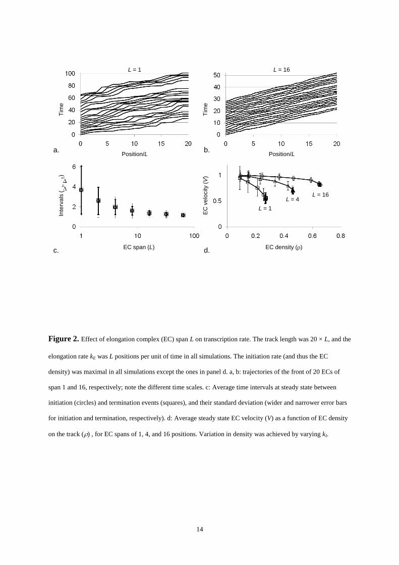
kI = 10.0), the rate at which new rounds start (the actual initiation rate) depends on the span L of the EC. Figure
2 compares the time trajectories of a group of 20 ECs, one group with L = 1, the other with L = 16, as they move
from down the track from position 1 to position 20 × L. In both cases, the first EC moves unhindered --albeit
somewhat erratically-- along an open track. However, owing to relatively slight random differences in velocity,
the next one occasionally runs into the one that was initiated first, and then has to wait until it can move
forward. This slows down its overall velocity, which has subsequent effects on the ECs that follow. It is
immediately clear, however, that the ECs with the larger span move much more smoothly: their dispersion
(deviation from a straight line) is significantly smaller. The difference in uniformity of motion is expected, as
movement over L is a single-step process for L = 1, but a 16-step sequential process if L spans 16 positions, with
time interval between individual steps exponentially distributed. The average time required for the EC to
complete L sequential steps with (equal) rate constants kE obeys a gamma distribution (Gibson, 2000) with a
mean of L/kE = 1.0 for both values of L, but a standard deviation of (L/kE2) equalling 1.0 for L = 1 (a gamma
distribution for L = 1 is an exponential distribution), but only 0.25 for L = 16. In all cases, a steady state, where
all ECs move at the same average velocity, appears to be reached quickly, but we routinely left the first 10
initiation and termination events out of the analysis to ensure that transient effects were not incorporated in the
statistics.
As a result of the difference in uniformity of motion, the average distance between the ECs on the track, and
therefore the average interval between consecutive initiation and termination events, I and T, is significantly
smaller for L = 16 than for L = 1: 1.4 0.2 (initiation) and 1.4 0.5 (termination) time units for L = 16 against
3.7 2.4 (initiation) and 3.7 2.6 (termination) time units for L = 1. Figure 2c shows that I and T, as well as
their variance I and T, decrease gradually to their limiting value of one time unit as L increases. The reciprocal
of T is the rate at which complete chains are produced (from here on referred to as the production rate, vP),
which is 0.3 0.2 per time unit for L = 1, and 0.9 0.2 for L = 64. Another measure for the efficiency of the
process is the average velocity V at which an EC completes an initiation-elongation-termination round,
computed from the time interval between its initiation and termination. If an EC has to wait frequently until its
forerunner has moved out of the way, its average velocity will be lower than when it can move unhindered.
9
Thus, V depends on the density of ECs on the track. The value of was varied by logarithmically increasing
the initiation frequency kI from 0.1 to 10.0, and computed from the termination frequency P ( = P/ Pmax
,
where Pmax
is the maximum value of P, 1.0). Figure 2d shows that V is close to its maximum value, 1.0, at low
densities ( < 0.1) but decreases for all values of L investigated, until a maximum density is reached. As
expected, ECs that move more smoothly achieve higher maximum densities and velocity.
Note that above we have compared ECs that, unhindered, travel their span L, rather than one position, in one
unit of time. It follows from Figure 2c that the maximum density of small ECs on a track of a particular length N
will always be greater than that of larger ones, irrespective of the level of congestion. However, results similar
to the above were obtained with models for which L = 1, but in which each translocation step (movement by one
position) consists of multiple consecutive reactions.
Relationship between activator or repressor binding site occupancy and production rate
As stated above, the activation condition may be interpreted as the instantaneous occupancy of the initiation
activator or repressor binding site (true indicates a bound activator, or unbound repressor). The average or
fractional occupancy over time of the binding site, , is modulated by keeping the firing rate of tA10, k10,
constant and varying that of tA01, k01:
R
d
A
d
A
d
KRKA
KA
kk
k
][1
1or
][1
][
1001
01Φ (3)
Thus, is dimensionless and varies between 0 (for k01 = 0) and 1 (for k10 = 0). Inside the brackets is a possible
interpretation of k01 and k10, where [A] and [R] are the concentrations of an activator A or repressor R, and KdA
and KdR are the dissociation equilibrium constants for the simplest possible activation or repression scenarios
(B + A AB (token in A1) or B + R AR (token in A0), where B is the binding site, and [A], [R] » 1). The
lifetime of the activated state (the average time it exists before becoming inactivated), A1, is equal to 1/k10, and
is changed, without affecting , by proportionally changing k01 and k10. To explore the relationship between
regulator site occupancy and production rate, we compare the dynamics of a system in which both kI and k10 are
fast with respect to the elongation rate kE with systems in which one is slow and the other fast. Systems in which
the value of kI is large (as compared with kE/L) have efficient initiation: provided the initiation condition remains
fulfilled, a new EC is ready to start elongating as soon as the previous one has moved out of the way. This is not
the case in systems in which kI is relatively small. Systems in which the lifetime of the activated state, 1/k10, is

10
short are responsive to changes in activator or repressor concentrations: when these concentrations change,
can adapt rapidly to the new condition. If the average lifetime of the activated state is long, adaptation will take
much longer.
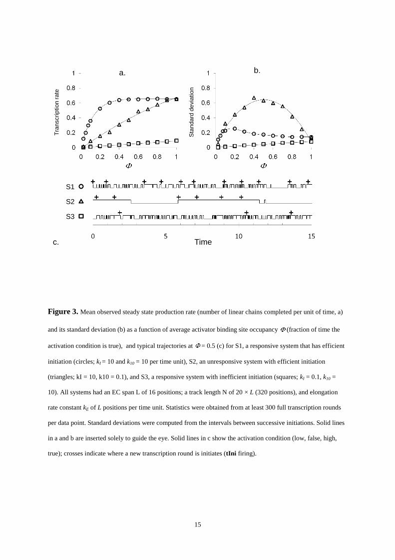
Figure 3 shows the results obtained for three extreme parameter sets, S1, S2, and S3. In S1, a responsive system
in which initiation is efficient, the observed production rate increases non-linearly with the regulatory site
occupancy, reaching a plateau at ≈ 0.4. When the plateau is reached, the standard deviation decreases to
approximately 30% as the intervals between successive initiations become more regular. The trajectory in panel
c, in which the activation state and tIni firing events are plotted over a period of 15 time units, reveals that, even
though the activation condition is only true for 50% of the time, the rapid alternation of “on” and “off” states
quickly creates new opportunities for new production rounds to begin once the previous EC has moved on.
However, if the activation complex is less dynamic, as in S2, or if the initiation system is not able to quickly
make use of opportunities to release a new EC, as in S3, the production rate becomes proportional to . In S2,
initiation is clustered inside the long periods in which the activation condition is true, and the completed linear
chains leave the track in bunches. Although owing to the high efficiency of the initiation process the intervals
between initiations within a cluster are regular, the intervals between the clusters are not, so that the overall
standard deviation on the observed production rate is very large (approaching 200% at = 0.5 in S2). In S3, on
the other hand, initiation is limiting and will only take a fraction of the opportunities that arise. As a result,
initiation events are exponentially distributed, and the observed production rate and its standard deviation have
the same value. Thus, S2 and S3 respond proportionally to changes in . Of course, the fact that, in most
activator or repressor binding scenarios, is non-linearly dependent on the actual activator or repressor
concentrations adds an extra layer of non-linearity. As the initiation process initiation is much more efficient in
S2 than in S3, S2 achieves the greater production rate. However, S2 cannot respond as rapidly to abrupt
“regime” changes, changes in activator or repressor concentrations in response to, e.g., received signals. Unless
a bound activator or repressor molecule is actively removed (which costs energy), the activated or repressed
state may extend unpredictably long into the new regime. S1, on the other hand, will respond rapidly, but is over
a large concentration range relatively insensitive to changes in activator or repressor concentrations.
Conclusion
Earlier models of template directed biological production processes are based on particle hopping schemes in
which the forward hopping probability is proportional to the average EC density on each position of the track.

11
The use of semaphores --which represent empty track positions and prevent EC from overtaking each other-- in
the model presented here simplifies the modelling procedure, and obviates the need for estimates of local
density. The visual nature of Petri-nets combined with the simple concept behind the stochastic First Reaction
method (Gillespie, 1977) help understanding the model and facilitate the interpretation of its complex dynamics.
These aspects may also encourage further analysis and the derivation of analytical expressions for observables
such as steady state flux and EC density, and comparison of the outcome with the results of earlier studies.
Acknowledgement
MJS thanks Prof. Wolfgang Marwan, Max Planck Institute for Dynamics of Complex Technical Systems,
Magdeburg, Germany, for introducing her to Petri-net modelling. This work was funded in part by a Wellcome
Trust Functional Genomics Development Initiative grant (ref. 072930/Z/03/Z).
References
Ackers, G.K., Johnson, A.D., Shea, M.A., 1982. Quantitative model for gene regulation by lambda phage
repressor. Proceedings of the National Academy of Sciences USA 79, 1129-1133.
Alon, U., 2006. An introduction to systems biology. Design principles of biological circuits, Chapman &
Hall/CRC, London.
Dijkstra, E.W. 2002 Cooperating sequential processes, in The origin of concurrent programming: from
semaphores to remote procedure calls, Springer-Verlag New York, Inc., pp 65-138.
Garai, A., Chowdhury, D., Ramakrishnan, T.V., 2009. Fluctuations in protein synthesis from a single RNA
template: Stochastic kinetics of ribosomes. Physical Review E 79, 011916-011916.
Gibson, M.A., Bruck, J., 2000. Efficient exact stochastic simulation of chemical systems with many species and
many channels. J. Phys. Chem. A. 104, 1876-1889.
Gillespie, D.T., 1977. Exact stochastic simulation of coupled chemical reactions. J. Phys. Chem. 81, 2340-2361.
Heinrich, R., Rapoport, T.A., 1980. Mathematical modelling of translation of mRNA in eucaryotes; steady
states, time-dependent processes and application to reticulocytest. Journal of Theoretical Biology 86,
279-313.
Lodish, H., Berk, A., Matsudaira, P., Kaiser, C.A., Krieger, M., Scott, M.P., Zipursky, S.L., Darnell, J., 2004.
Molecular Cell Biology, 5th ed., W. H. Freeman & Company, New York, NY.
MacDonald, C.T., Gibbs, J.H., Pipkin, A.C., 1968. Kinetics of biopolymerization on nucleic acid templates.
Biopolymers 6, 1-25.
MacDonald, C.T., Gibbs, J.H., 1969. Concerning the kinetics of polypeptide synthesis on polyribosomes.
Biopolymers 7, 707-725.
Petri, C.A., 1962 Kommunikation mit Automaten, Schriften des IIM Nr. 2, in Institut für Instrumentelle
Mathematik, Bonn
Schilstra, M.J., Martin, S.R. 2009 Simple Stochastic Simulation, in Methods in Enzymology (Michael, L.J.,
Ludwig, B., Eds.), Academic Press, pp 381-409.
Shea, M.A., Ackers, G.K., 1985. The OR control system of bacteriophage lambda : A physical-chemical model
for gene regulation. Journal of Molecular Biology 181, 211.
Wilkinson, D.J., 2006. Stochastic Modelling for Systems Biology, Chapman & Hall/CRC, London, UK.
Zouridis, H., Hatzimanikatis, V., 2007. A Model for Protein Translation: Polysome Self-Organization Leads to
Maximum Protein Synthesis Rates. Biophysical Journal 92, 717-730.
12
Figure Legends
Figure 1. Petri-net model of a biological template-directed linear production process, such as DNA replication
or transcription, or mRNA translation. Open circles, places; black or grey disks inside places, tokens; rectangles,
transitions (open: disabled, grey: enabled); arrows, arcs; rounded rectangles, layers. T, DNA template layer; E,
elongation layer; A, activation/initiation layer; C, completion (termination) layer. The N places in layers E and T
are numbered E1, E2, ...EN, and T1, T2, ...TN; the (unlabeled) transitions in E and A are identified as tE1,2, tE2,3,
...tEN-1,N, and tA0,1 and tA1,0, respectively. Rate constants associated with tIni, tTerm, tA0,1, tA1,0, and tEj,j+1 are
named kI, kT, k01, k10, and kEj,j+1, respectively.
Figure 2. Effect of elongation complex (EC) span L on transcription rate. The track length was 20 × L, and the
elongation rate kE was L positions per unit of time in all simulations. The initiation rate (and thus the EC
density) was maximal in all simulations except the ones in panel d. a, b: trajectories of the front of 20 ECs of
span 1 and 16, respectively; note the different time scales. c: Average time intervals at steady state between
initiation (circles) and termination events (squares), and their standard deviation (wider and narrower error bars
for initiation and termination, respectively). d: Average steady state EC velocity (V) as a function of EC density
on the track ( ) , for EC spans of 1, 4, and 16 positions. Variation in density was achieved by varying kI.
Figure 3. Mean observed steady state production rate (number of linear chains completed per unit of time, a)
and its standard deviation (b) as a function of average activator binding site occupancy (fraction of time the
activation condition is true), and typical trajectories at = 0.5 (c) for S1, a responsive system that has efficient
initiation (circles; kI = 10 and k10 = 10 per time unit), S2, an unresponsive system with efficient initiation
(triangles; kI = 10, k10 = 0.1), and S3, a responsive system with inefficient initiation (squares; kI = 0.1, k10 =
10). All systems had an EC span L of 16 positions; a track length N of 20 × L (320 positions), and elongation
rate constant kE of L positions per time unit. Statistics were obtained from at least 300 full transcription rounds
per data point. Standard deviations were computed from the intervals between successive initiations. Solid lines
in a and b are inserted solely to guide the eye. Solid lines in c show the activation condition (low, false, high,
true); crosses indicate where a new transcription round is initiates (tIni firing).

13
Figure 1. Petri-net model of a biological template-directed linear production process, such as DNA replication
or transcription, or mRNA translation. Open circles, places; black or grey disks inside places, tokens; rectangles,
transitions (open: disabled, grey: enabled); arrows, arcs; rounded rectangles, layers. T, DNA template layer; E,
elongation layer; A, activation/initiation layer; C, completion (termination) layer. The N places in layers E and T
are numbered E1, E2, ...EN, and T1, T2, ...TN; the (unlabeled) transitions in E and A are identified as tE1,2, tE2,3,
...tEN-1,N, and tA0,1 and tA1,0, respectively. Rate constants associated with tIni, tTerm, tA0,1, tA1,0, and tEj,j+1 are
named kI, kT, k01, k10, and kEj,j+1, respectively.
E
A CT
1 2 3 4 5 N-1 N
1
0
tIni
tTerm
N-2..........
14
Figure 2. Effect of elongation complex (EC) span L on transcription rate. The track length was 20 × L, and the
elongation rate kE was L positions per unit of time in all simulations. The initiation rate (and thus the EC
density) was maximal in all simulations except the ones in panel d. a, b: trajectories of the front of 20 ECs of
span 1 and 16, respectively; note the different time scales. c: Average time intervals at steady state between
initiation (circles) and termination events (squares), and their standard deviation (wider and narrower error bars
for initiation and termination, respectively). d: Average steady state EC velocity (V) as a function of EC density
on the track ( ) , for EC spans of 1, 4, and 16 positions. Variation in density was achieved by varying kI.
L = 1
L = 4L = 16
Tim
e
Tim
e
Position/L Position/L
L = 1 L = 16
EC span (L) EC density ( )
EC
ve
locity (
V)
Inte
rva
ls (
I, T)
a. b.
c. d.
15
Figure 3. Mean observed steady state production rate (number of linear chains completed per unit of time, a)
and its standard deviation (b) as a function of average activator binding site occupancy (fraction of time the
activation condition is true), and typical trajectories at = 0.5 (c) for S1, a responsive system that has efficient
initiation (circles; kI = 10 and k10 = 10 per time unit), S2, an unresponsive system with efficient initiation
(triangles; kI = 10, k10 = 0.1), and S3, a responsive system with inefficient initiation (squares; kI = 0.1, k10 =
10). All systems had an EC span L of 16 positions; a track length N of 20 × L (320 positions), and elongation
rate constant kE of L positions per time unit. Statistics were obtained from at least 300 full transcription rounds
per data point. Standard deviations were computed from the intervals between successive initiations. Solid lines
in a and b are inserted solely to guide the eye. Solid lines in c show the activation condition (low, false, high,
true); crosses indicate where a new transcription round is initiates (tIni firing).
Tra
nscri
ptio
n r
ate
Sta
nd
ard
de
via
tio
n
a. b.
c. Time
S1
S2
S3