stochastic reserving – case study using a bayesian … · stochastic reserving – case study...

Stochastic reserving – case study

using a Bayesian approach

Prepared by Bartosz Piwcewicz

Presented to the Institute of Actuaries of Australia 16th General Insurance Seminar 9-12 November 2008

Coolum, Australia

This paper has been prepared for the Institute of Actuaries of Australia’s (Institute) XVIth General Insurance Seminar 2008.

The Institute Council wishes it to be understood that opinions put forward herein are not necessarily those of the

Institute and the Council is not responsible for those opinions.

Bartosz Piwcewicz

The Institute will ensure that all reproductions of the paper acknowledge the Author/s as the author/s, and include the above copyright statement:

The Institute of Actuaries of Australia

Level 7 Challis House 4 Martin Place

Sydney NSW Australia 2000

Telephone: +61 2 9233 3466 Facsimile: +61 2 9233 3446

Email: [email protected] Website: www.actuaries.asn.au

Stochastic reserving – case study using a Bayesian approach

of 26

Abstract There are a number of quantitative approaches used for stochastic reserving, uncertainty assessment and risk margin modelling in general insurance. Australian actuaries are quite familiar with techniques such as bootstrapping, stochastic chain ladder or the Mack method. However, the Bayesian approach to stochastic reserving is not well as understood in the actuarial community. This approach is relatively new and has been extensively researched overseas. This paper aims to introduce the Bayesian approach to those unfamiliar with it in the context of stochastic reserving. The discussion is supported by a case study and suggestions on how the theory can be deployed in practice. Keywords: Bayesian approach, stochastic reserving; risk margins;


of 26

Table of Contents

1. Introduction.........................................................................................................................4 2. Overview of the theory .......................................................................................................5

2.1. General Bayesian modelling process......................................................................5 2.2. Mathematics of the Bayesian approach ..................................................................7 2.3. A non-reserving example ........................................................................................8 2.4. MCMC methods and the Gibbs sampler .................................................................9 2.5. Advantages and disadvantages ............................................................................11

3. Case study .......................................................................................................................13 3.1. Overview of implemented models and the modelling strategy..............................13 3.2. Data .......................................................................................................................16 3.3. Stochastic modelling results..................................................................................16

4. Summary and conclusions ...............................................................................................19 5. Acknowledgements ..........................................................................................................20 6. Appendix ..........................................................................................................................21 7. Bibliography......................................................................................................................25


of 26

1. Introduction

Actuaries recognised the difficulty involved in the estimation of general insurance liabilities a long time ago. The first actuarial research papers considering the uncertainty inherent in the general insurance reserving process were written in the early 1980s. In essence, stochastic reserving is an attempt to quantify this uncertainty and estimate the distribution underlying the reserves for a particular insurance portfolio. The scope of stochastic reserving is broader than for traditional reserving methods, which are generally concerned with the estimation of a central estimate (ie. the mean of the underlying distribution of outcomes). While discussing stochastic reserving, it is important to differentiate between a model and the approach which is used to implement this model. In this context, the model is a statistical model describing the underlying insurance claim process (e.g. the over-dispersed Poisson) and the approach is a method/technique used to deploy such a model in a particular reserving situation (e.g. assessing uncertainties inherent in the past data). Arguably there is no single model that suits all reserving problems. A robust approach should be flexible enough to accommodate any model and perform well in all reserving situations. In Australia, stochastic reserving has come under increased scrutiny following the 2002 APRA reforms and the introduction of a requirement to include a risk margin in the provision for insurance liabilities for regulatory purposes. Most recently, APRA has also released guidelines regarding internal economic capital models. This more recent development may encourage further research into and use of stochastic reserving techniques. The purpose of this paper is to present a stochastic reserving framework that uses Bayesian techniques (Bayesian stochastic reserving). Bayesian stochastic reserving has been extensively researched overseas but not in Australia. In particular, the paper will address the following main topics in the context of a reserving case study:

• an overview of the mechanics and theory underlying Bayesian stochastic reserving; and

• an illustration of how two reserving actuarial methods, the chain ladder and Bornhuetter-Ferguson methods, can be implemented using this approach.

Although the case study presents an implementation of the Bayesian approach in the context of outstanding claim liabilities, this approach can be equally used for premium (or unexpired risk) liabilities. The paper is essentially structured into two main parts. The first part gives an overview of key theoretical concepts underpinning Bayesian stochastic reserving. The second part presents an application of this approach to a reserving case study using the statistical software package WinBUGS. The paper is concluded with an Appendix showing the WinBUGS code used for the case study.


of 26

2. Overview of the theory

In the past, the implementation of Bayesian approaches has been limited by the lack of efficient computational/sampling methods. Developments in computing power and some significant advances in the understanding of sampling algorithms in the early 1990s led to an increase in the application of Bayesian approaches to a wide range of practical problems, including stochastic reserving. Since then a number of papers on Bayesian stochastic reserving have been written outlining Bayes’ theory and proposing various Bayesian models. I have included some of these papers in the Bibliography section. I encourage readers interested in obtaining a thorough understanding of Bayesian stochastic reserving to read the following papers: de Alba [6], England and Verrall [10], Ntzoufras and Dellaportas [17], Scollnik[22], Verrall [23] and Verrall and England [24]. I consider these papers to provide a good description of the theory and so I have limited my discussion in this section of the paper to a high-level outline of the key concepts and mechanisms and concluded with a discussion of the advantages and disadvantages of Bayesian stochastic reserving.

2.1. General Bayesian modelling process

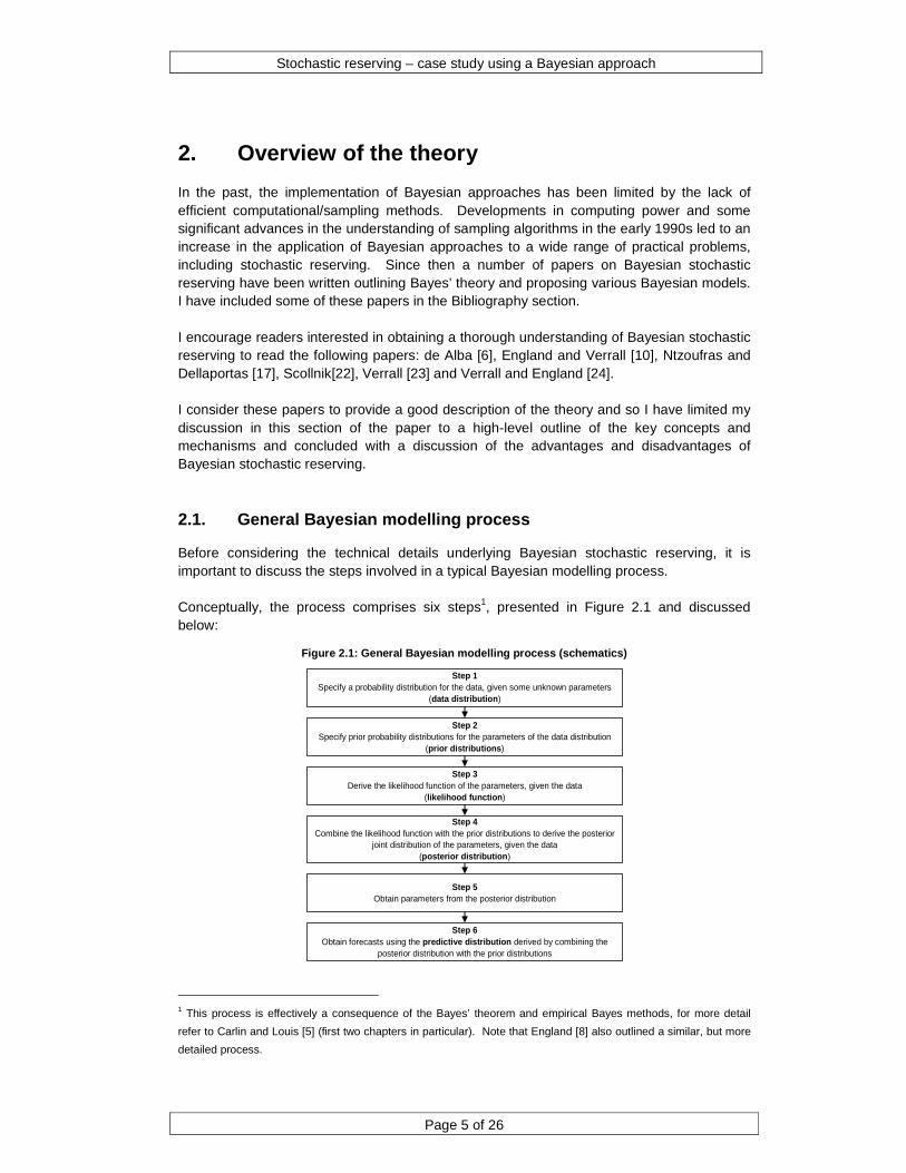
Before considering the technical details underlying Bayesian stochastic reserving, it is important to discuss the steps involved in a typical Bayesian modelling process. Conceptually, the process comprises six steps1, presented in Figure 2.1 and discussed below:

Figure 2.1: General Bayesian modelling process (schematics)

Step 1Specify a probability distribution for the data, given some unknown parameters

(data distribution)

Step 2Specify prior probability distributions for the parameters of the data distribution

(prior distributions)

Step 3Derive the likelihood function of the parameters, given the data

(likelihood function)

Step 4Combine the likelihood function with the prior distributions to derive the posterior

joint distribution of the parameters, given the data(posterior distribution)

Step 5Obtain parameters from the posterior distribution

Step 6Obtain forecasts using the predictive distribution derived by combining the

posterior distribution with the prior distributions

1 This process is effectively a consequence of the Bayes’ theorem and empirical Bayes methods, for more detail

refer to Carlin and Louis [5] (first two chapters in particular). Note that England [8] also outlined a similar, but more

detailed process.

of 26

The first two steps are concerned with the specification of a statistical model. An example of such a model could be the over-dispersed Poisson model (ODP model) implemented in the second part of this paper or any other statistical model defined in terms of steps 1 and 2. A detailed discussion of how to select an appropriate statistical model given a particular reserving situation is outside the scope of this paper. However this process would involve a degree of actuarial judgement and some goodness of fit testing. While the data distribution is likely to be completely defined by a particular statistical model (e.g. ODP distribution in the ODP model), the specification of prior distributions for the model parameters can be quite flexible. For example, one can use non-informative (or vague) prior distributions, where parameters have large variances and do not contribute any information to the posterior distribution. Alternatively, informative (or strong) prior distributions could be used for which parameters have small variances and so influence the shape of the posterior distribution. For some statistical models, it is also possible to assume different statistical distributions for prior distributions (e.g. Gamma, Normal, Lognormal etc.), further influencing the shape of the posterior distribution. Step 4 essentially leads to the estimation of the posterior distribution and arises from the application of Bayes’ theory. The key is that the posterior distribution is proportional to the product of the likelihood function and the prior distributions2. The complexity of step 5 depends on two main factors: the number of parameters underlying a particular statistical model and the shape of the posterior distribution. If there is only one parameter and the posterior distribution can be easily recognised as a standard statistical distribution the estimation of the parameter is fairly straightforward as shown in section 2.3. However, if there are multiple parameters and the posterior distribution is not recognisable, as is the case for the majority of actuarial statistical models, the derivation of the parameters requires a special sampling algorithm. Markov chain Monte Carlo (MCMC) methods have proven very useful in this context. Section 2.4 gives an overview of one such sampling technique, the Gibbs sampler. In the last step, the forecasts of new observations not included in the existing dataset are obtained, including parameter and process error. As for step 5, the complexity associated with forecasting varies considerably depending on whether the predictive distribution is recognisable. If the predictive distribution is recognisable, as in the example presented in section 2.3, the required parameters of the predictive distribution can be estimated directly and the new observations are straightforward to obtain. If however this distribution is not a standard statistical distribution it is necessary to simulate the new observations from the data distribution, conditional on the simulated (in step 5) parameters. This process requires a generic sampling algorithm such as Adaptive Rejection Sampling3 (ARS), which generates samples from non-standard statistical distributions. As an extension of step 6, it is also possible to assume a particular standard statistical distribution as the predictive distribution and use the output from a generic sampler to parameterise it. For example, England and Verrall [10] used the Gamma distribution as the predictive distribution in their implementation of the ODP model.

2 For more detail see http://en.wikipedia.org/wiki/Posterior_probability, and the expression of the Bayes' theorem in

terms of likelihood shown in http://en.wikipedia.org/wiki/Bayes%27_theorem 3 For more detail see Gilks and Wild [13]

of 26

2.2. Mathematics of the Bayesian approach

Bayes’ theory will be described here very briefly and my main focus is on its application to stochastic reserving. For a comprehensive discussion on Bayes’ theory and methods, the reader is referred to statistics textbooks (e.g. Berger [2], Bernardo and Smith [3] or Carlin and Louis [5]). In probability theory, Bayes' theorem considers the conditional and marginal probabilities of two random events and it can be stated in a number of different ways. For stochastic reserving, the most convenient presentation is in terms of probability distribution functions and the likelihood function. Let’s consider a simple reserving project shown in Table 2.1, where {Cij: i= 1, …, n; j= 1, …, n} are random variables representing claim payments or any other data commonly used in actuarial triangulation analysis.

Table 2.1: Example of a reserving project

1 2 3 … n

1 C 11 C 12 C 13 … C 1n

2 C 21 C 22 C 23 … C 2n

3 C 31 C 32 C 33 … C 3n

… … … … … …

n C n1 C n2 C n3 … C nn

Development periodOrigin Period

If we further note that c={Cij: i + j ≤ n + 1} is the upper-left triangle incorporating the observed payment (or other) data, the reserving problem is to estimate the unobserved values in the lower-right triangle. Using the notation of Bayes’ theory4 and the general step-by-step process introduced in section 2.1, this reserving problem can be approached as follows:

• Steps 1 to 2: Assume that each Cij (whether in the upper-left or lower-right triangle) follows a probability distribution f(Cij/θ), where θ denotes a vector of parameters describing a particular claim process generating Cij, and all parameters are distributed according to a prior distribution function π(θ).

• Steps 3: Calculate the likelihood function L(θ/c) for the parameters given the observed data:

( ) ( )∏ +≤+=

1//

nji ijCfL θcθ

• Steps 4: Given the data distribution and the prior distribution, the posterior distribution f(θ/c) is proportional to the product of the likelihood function and the prior distribution:

4 For example see http://en.wikipedia.org/wiki/Bayes_theorem and the bibliography referred to on this website

of 26

( ) ( ) ( )θcθcθ π/L/f ∝

• Steps 5: Parameters θ are obtained from f(θ/c) and used in the next step.

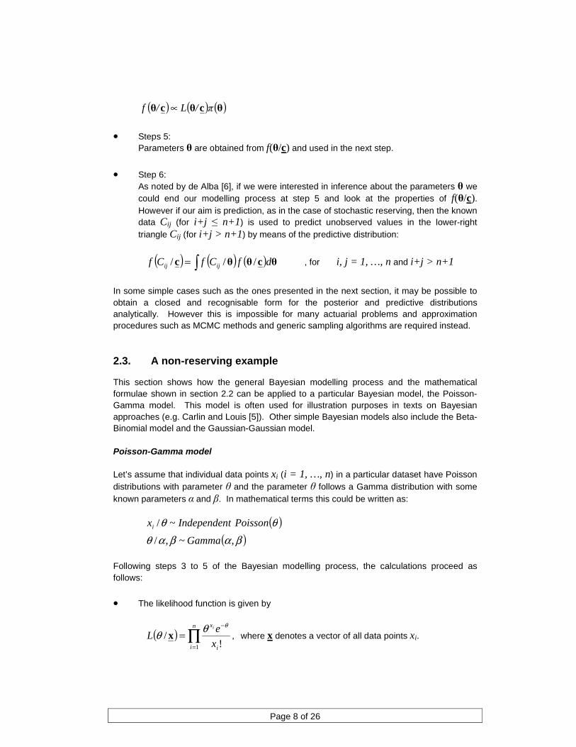
• Step 6: As noted by de Alba [6], if we were interested in inference about the parameters θ we could end our modelling process at step 5 and look at the properties of f(θ/c). However if our aim is prediction, as in the case of stochastic reserving, then the known data Cij (for i+j ≤ n+1) is used to predict unobserved values in the lower-right triangle Cij (for i+j > n+1) by means of the predictive distribution:

( ) ( ) ( )∫= θcθθc dfCfCf ijij /// , for i, j = 1, …, n and i+j > n+1

In some simple cases such as the ones presented in the next section, it may be possible to obtain a closed and recognisable form for the posterior and predictive distributions analytically. However this is impossible for many actuarial problems and approximation procedures such as MCMC methods and generic sampling algorithms are required instead.

2.3. A non-reserving example

This section shows how the general Bayesian modelling process and the mathematical formulae shown in section 2.2 can be applied to a particular Bayesian model, the Poisson-Gamma model. This model is often used for illustration purposes in texts on Bayesian approaches (e.g. Carlin and Louis [5]). Other simple Bayesian models also include the Beta-Binomial model and the Gaussian-Gaussian model. Poisson-Gamma model Let’s assume that individual data points xi (i = 1, …, n) in a particular dataset have Poisson distributions with parameter θ and the parameter θ follows a Gamma distribution with some known parameters α and β. In mathematical terms this could be written as:

( )( )βαβαθ

θθ,~,/

~/

Gamma

PoissontIndependenxi

Following steps 3 to 5 of the Bayesian modelling process, the calculations proceed as follows:

• The likelihood function is given by

( ) ∏=

−

=n

i i

x

x

eL

i

1 !/

θθθ x , where x denotes a vector of all data points xi.

of 26

• The posterior distribution is proportional to the product of this likelihood function and the prior distribution:

( ) ( )βθα

αθ

θα

βθβαθ −−

=

−

Γ

∝ ∏ e

x

ef

n

i i

xi1

1 !,,/ x ,

and this can be simplified as

( ) θβα

θβαθ )(1

1,,/ nx

ef

n

ii

+−−+∑

∝ =x .

• The simplified expression on the right hand side can be recognised as a Gamma distribution:

+∑+

=nxGamma

n

ii βαβαθ ,~,,/

1x

• In the final step we obtain the predictive distribution for forecasting x~ , new data points not included in the existing data set. This is achieved by integrating the product of the Poisson distribution for the data and the posterior Gamma distribution. The resulting predictive distribution is

( ) ( )( ) ( )

x

x

xxf

~

11

1

1

1

1

1

11~

~/~

1

+

++ΓΓ

+Γ=ββ

βα

αα

x ,

where ∑+==

n

iix

11 αα and n+= ββ1

This distribution can be recognised as a Negative Binomial distribution with parameters y and q

( )qynomialNegativeBix ,~~ , where 1α=y and 11

1

β+=q

2.4. MCMC methods and the Gibbs sampler

The discussion in this section largely follows Walsh [25], who gives a good and fairly detailed description of MCMC methods, including the Gibbs sampler5. My intention is to present here a high-level overview of the Gibbs sampling approach and illustrate it with a general example. As noted in section 2.1, Gibbs sampling could be used in step 5 of the general Bayesian modelling process. The key difficulty with the application of Bayesian methods is the ability to sample from a joint posterior distribution of parameters. This task becomes particularly complicated if there

5 The Gibbs sampler was initially developed in the context of image processing (Geman and Geman [11]). Gelfand

and Smith [12] then showed how the method could be applied to a wider range of Bayesian problems.

of 26

are multiple parameters and the distribution itself is non-standard. MCMC methods have been developed to tackle such practical implementation problems efficiently. In order to illustrate how the Gibbs sampler tackles this problem let us consider a bivariate joint distribution f(x,y), for which we wish to derive one or both marginal distributions, f(x) and f(y). The key to the Gibbs algorithm is that it only considers univariate conditional distributions (ie. f(x/y) and f(y/x)), which are far easier to compute than the marginal distributions via integration of the joint density (e.g. f(x) = ∫ f(x,y)dy). In other words, this

bivariate problem is broken up into a sequence of univariate problems. The sampler starts with some initial arbitrary value y0 for y and obtains x0 by generating a random variable from the conditional distribution f(x/y = y0). The sampler then uses x0 to generate a new value of y1, drawing from the conditional distribution based on the value x0, f(y/x = x0). If f(x/y) and f(y/x)) are standard statistical distributions (e.g. Gamma) then these draws are fairly straightforward to obtain. However, if these distributions are non-standard then Gibbs sampling is combined with a generic sampling algorithm such as ARS or more efficient Random Walk Metropolis algorithms6 to draw randomly from the conditional distributions. If this process runs for k iterations a k x 2 grid with values is populated, where the rows of the grid relate to iterations of the Gibbs sampler, and the columns relate to variables x and y. The sampling process is as follows:

( )1/~ −= ii yyxfx

( )ii xxyfy =/~

It is worth highlighting that at each iteration only the most recent information to date for the other variable is used, which is the same as in case of a Markov chain. Once a sufficient number of draws (so called “burn-in” sample) is simulated from the joint distribution, the Gibbs sequence converges to a stationary (equilibrium or target) distribution that is independent of the starting/initial values. In practice, it is common to run the sampler for an additional m simulations after the burn-in thus ensuring a random sample from the joint distribution. An alternative approach would be to generate several samples of length m each starting from a different initial value. There are a number of convergence diagnostics used to assess whether a Gibbs sample has converged. These include some formal tests such as the Geweke test or the Raftery-Lewis test7. However, one should always visually inspect parameter values generated by the Gibbs sampler plotted against the number of iterations and/or check the autocorrelation in the simulated sample of parameter values. It is worth noting that these and other tests are readily available within WinBUGS. The Gibbs sampler has been implemented in a statistical software WinBUGS developed by the MRC Biostatistics Unit at the University of Cambridge. The BUGS (Bayesian inference Using Gibbs Sampling) project started in 1989 and its key purpose has been to design a

6 E.g. Adaptive Rejection Metropolis Sampling (Gilks, Best and Tan [14]) 7 See Walsh [25] for a description of these tests

of 26

flexible software for the Bayesian analysis of complex statistical models using MCMC methods. The BUGS Project website is found at www.mrc-bsu.cam.ac.uk/bugs/ . The WinBUGS software is supplemented with an extensive manual including examples and tips on how a Bayesian model can be implemented within WinBUGS. In addition, there have been a number of papers discussing the use of WinBUGS in the context of various actuarial applications (e.g. Scollnik [21]). Although WinBUGS is a robust and fairly straightforward software to use, it is not free from some practical implementation issues e.g.:

• Standard statistical distributions and models are easy to implement within WinBUGS. For non-standard distributions some workaround is required using the so-called “zeros” or “ones” tricks.

• There can be considerable numerical overflow/underflow issues, slowing down the simulation process or in some cases making it impossible to run. It is often a good idea to scale down or up all numbers, so there are no very large or very small values handled by WinBUGS.

• The error messages are sometimes quite unhelpful.

2.5. Advantages and disadvantages

Concluding the theoretical part of the paper, it is important to consider some key properties of Bayesian stochastic reserving (both advantages and possible disadvantages). These are summarised in Table 2.2 below.

Table 2.2: Advantages and disadvantages of Bayesian stochastic reserving

Advantages Disadvantages

• Requires a completely specified statistical model, ensuring clarity of underlying assumptions

• Flexible in application and not limited to any particular model

• Allows explicit modelling of various sources of uncertainty

• Allows incorporation of adjustment for uncertainties not included in the past data

• Automatically produces full distribution of outcomes

• Does not generate pseudo data and so is not impacted by issues sometimes affecting bootstrapping (e.g. a limited set of combinations of residuals, the possibility of negative pseudo-data at the start of a triangle)

• Fairly easy to implement using either WinBUGS or a variety of programming languages, once the underlying theory is understood

• Theoretically more sophisticated approach

• The mechanism underlying the Bayesian approach is less open to manipulation than bootstrapping methods8

• Selection of prior distributions may be problematic

• May be seen as a “black box” approach

8 Note that this disadvantage could be also seen as an advantage, since it limits implementation errors.

of 26

The above table shows that Bayesian stochastic reserving offers some benefits compared to other stochastic reserving methods. In particular, this approach is more flexible than for example the bootstrapping approach. England and Verrall [10] showed that the Bayesian and bootstrapping approaches essentially produce the same results, when non-informative prior distributions are used within the Bayesian approach. However if one would like to incorporate judgement regarding parameters/parameter distributions underlying a particular statistical model or combine together several statistical models, the Bayesian approach is the preferred (or in most cases the only) option. Any stochastic reserving technique only incorporates uncertainties inherent in the past data and an allowance for any other uncertainties is often made separately. The key benefit of the Bayesian approach is that it provides a flexible and sound mechanism to allow for these other uncertainties. Actuarial judgement and external information regarding uncertainties not reflected in the past data can be allowed for within Bayesian stochastic reserving in a number of ways and there are papers that have shown some examples of such implementations e.g.:

• Verrall and England [24] showed how external information and actuarial judgement could be incorporated in the development factors for a particular Bayesian model (the Negative Binomial model) underlying the chain ladder method.

• Verrall [23] showed how external information and actuarial judgement about accident years could be incorporated into two Bayesian models (the Negative Binomial and Over-dispersed Poisson models) using the mechanism of the Bornhuetter-Ferguson method.

• Scollnik [22] also showed how the mechanism of the Bornhuetter-Ferguson method could be used to incorporate external information and actuarial judgement about accident years into the distribution of outstanding losses. Note that this method has been applied in the case study in the second part of this paper.

Although the above papers are quite comprehensive, I acknowledge that there is still more research to be conducted in this area. The key disadvantage of Bayesian stochastic reserving, which may discourage actuaries from choosing this approach, is its apparent complexity compared to other stochastic reserving methods. The mathematics looks quite complicated and the implementation may require some sophisticated sampling algorithms (e.g. MCMC methods or ARS). However, I believe that once some basic concepts from Bayes’ theory are understood, the implementation becomes fairly straightforward, especially when one uses WinBUGS or other software e.g. Igloo with ExtrEMB [16].


of 26

3. Case study

This part of the paper presents an application of the Bayesian approach in a stochastic reserving context. All modelling for the purpose of this case study has been conducted using WinBUGS. The WinBUGS code used is shown in the Appendix. The case study uses a triangulation of claim payments relating to Automatic Facultative General Liability (excluding Asbestos and Environmental) from the Historical Loss Development Study [15], previously used by other authors including England and Verrall [9] and Verrall [23]. In addition, I have created dummy earned premiums for each accident year. The triangle and earned premiums are shown in Table 3.1.

3.1. Overview of implemented models and the modelling strategy

This section essentially follows the general Bayesian modelling process discussed in section 2.1, unless noted otherwise. In order to present Bayesian stochastic reserving in the most accessible way, I have chosen a fairly straightforward statistical model underlying the chain ladder method. This model has then been extended using the mechanics of the Bornhuetter-Ferguson method incorporated within a Bayesian approach. The statistical chain ladder model is specified as an ODP model, defined by Renshaw and Verrall [19]. The Bayesian Bornhuetter-Ferguson extension (BF model) is based on an approach previously considered by Scollnik [22].

Over-Dispersed Poisson Chain Ladder Model

The key to the ODP model is the derivation of the over-dispersed Poisson distribution, which follows from an observation that if X ~ Poisson (µ), then Y=φX has the over-dispersed Poisson distribution, with mean φµ and variance φ2µ. φ is called the over-dispersion parameter and is generally greater than 1. The ODP model for the chain ladder method can be specified as follows:

~,,/ ϕyxijC independent over-dispersed Poisson, with mean xi yj, and ∑=

=n

jjy

1

1

~, ji yx independent non-informative Gamma distributions9

x and y are parameter vectors relating to the rows (origin years 1, …, n) and columns (development years 1, …, n), respectively, of the data triangle. The row parameters xi can be interpreted as expected ultimate claims cost for the i-th accident year and the column parameters yj as the proportion of ultimate claims emerging in the j-th development year. The above specification means that past and future incremental payments follow independent over-dispersed Poisson and the row and column parameters have non-informative prior distributions. For simplicity, the over-dispersion parameter φ is constant across all development periods and estimated outside the model using maximum likelihood estimation. As an alternative, one could assume φ varies by development year (as shown

9 Refer to the WinBUGS code for details

of 26

by England and Verrall [10]) and/or follows some prior distribution10 as is the case for the row and column parameters. Using the general Bayesian notation introduced in section 2.2 and consistent with steps 5 and 6 of the general Bayesian modelling process:

• The posterior distribution for the row and column parameters satisfies the following proportionality:

( ) ( ) ( ) ( )∏ +≤+∝

1,,/,/,

nji ijCff yxyxcyx ππϕϕ

• For the unobserved values in the lower-right triangle CLijC (for i+j > n+1), the

predictive distributions are:

( ) ( ) ( )∫∫= yxcyxyxc ddfCfCf ijCLij ϕϕϕ ,/,,,/,/

Since the posterior distribution f(x,y/c,φ) cannot be recognised as a standard statistical distribution and there are multiple parameters, it is necessary to implement this model in WinBUGS, where the Gibbs sampler along with ARS are used to generate random draws of row and column parameters from this distribution. The generated parameters are

incorporated into the ODP distributions for unobserved values CLijC to derive the distribution

of undiscounted outstanding claims11.

Bornhuetter-Ferguson Model

As already noted, the BF model is an extension of the chain ladder model. The basic mechanism to derive the ultimate claims cost for each i-th accident year is consistent with the Bornhuetter-Ferguson method (Bornhuetter and Ferguson [4]) and I assume that the reader is already familiar with this approach. The stochastic element is added to the Bornhuetter-Ferguson method via assumed ultimate loss ratios for each accident year. In addition, the proportions of the BF-based ultimate claims cost emerging in each j-th development year are derived from the chain ladder factors simulated as part of the ODP model.

The modelling process to obtain the unobserved values BFijC (for i+j > n+1) is slightly

different from the general Bayesian modelling process described in section 2.1. For this reason, I include here a more detailed explanation of the various steps of this process.

10 Such an approach was proposed by Scollnik (see Antonio, Beirlant and Hoedemakers [1]), where φ was treated

as the third parameter in the ODP model and followed a Gamma distribution. 11 For completeness, it is worth noting that the implementation in WinBUGS uses “a quasi-likelihood approach” so

that the observed and future payments are not restricted to positive integers. See Verrall [23] and England and

Verrall [10] for more discussion.

of 26

The prior parameters of the model are the initial ultimate loss ratios IniiLR based on some

external knowledge. The observed data are the ultimate loss ratios obtained using the ODP

model ODPiLR . The statistical model is specified as follows:

( )( )i

Inii

Inii

ODPi

iiInii

LRNormaltIndependenLRLR

NormaltIndependenLR

)2(

)1(

,~/

,~

σ

σµ12

Although the data distribution (of Inii

ODPi LRLR / ) assumes Normality, the ODP

iLR

unconditional on the IniiLR are derived from the ODP chain ladder model.

The posterior distribution ( )ODPi

Inii LRLRf / is obtained as follows:

( ) ( ) ( )Inii

ODPi

Inii

ODPi

Inii LRfLRLRLLRLRf // ∝

The specification of the model and the non-Normal distribution of ODPiLR unconditional on

IniiLR mean that this posterior distribution ( )ODP

iInii LRLRf / is complex and the Gibbs

sampler and ARS within WinBUGS are required to generate samples of the assumed ultimate loss ratios, ie. the initial ultimate loss ratios conditional on the ODP-based ultimate loss ratios. The simulated assumed ultimate loss ratios are applied to earned premiums to derive BF-

based ultimate claim costs across different accident years. The unobserved values BFijC (for

i+j > n+1) are then obtained by applying the chain ladder factors simulated as part of the

ODP model. It is worth noting that these factors are consistent with the ODPiLR used to

obtain the posterior distribution ( )ODPi

Inii LRLRf / .

It is also important to highlight a particular credibility mechanism implemented within the BF model. The relativity between standard deviations of the two normal distributions controls how much weight is given to the initial ultimate loss ratios and to the ODP-based ultimate

loss ratios.13 If standard deviations σ(2)i selected for the normal distribution of Inii

ODPi LRLR /

are relatively lower than σ(1)i the resulting assumed ultimate loss ratios are closer to the simulated ODP-based ultimate loss ratios.

12 For the purpose of the case study, I have arbitrarily assumed that standard deviations for both normal

distributions are equal to 7.1% and the mean of the distribution of initial ultimate loss ratios is 71% across all

accident years. This mean has been based on the total ultimate loss ratio implied by the deterministic chain ladder

(see Table 3.1). 13 Note that this relativity is expressed by the weight parameter in the WinBUGS code.

of 26

3.2. Data

Table 3.1 shows a triangle of incremental payments with reserves estimated using the deterministic chain ladder. Earned premiums, ultimate loss ratios and chain ladder factors are also shown.

Table 3.1: Case study – incremental claim payments and deterministic chain ladder results

1 2 3 4 5 6 7 8 9 10

1 5,012 3,257 2,638 898 1,734 2,642 1,828 599 54 172 0 28,975 65%2 106 4,179 1,111 5,270 3,116 1,817 -103 673 535 154 20,478 82%3 3,410 5,582 4,881 2,268 2,594 3,479 649 603 617 28,984 83%4 5,655 5,900 4,211 5,500 2,159 2,658 984 1,636 38,432 75%5 1,092 8,473 6,271 6,333 3,786 225 2,747 47,290 61%6 1,513 4,932 5,257 1,233 2,917 3,649 24,308 80%7 557 3,463 6,926 1,368 5,435 23,228 76%8 1,351 5,596 6,165 10,907 30,721 78%9 3,133 2,262 10,650 29,611 54%

10 2,063 16,339 29,407 63%

52,135 301,434 71%Chain ladder factors 2.9994 1.6235 1.2709 1.1717 1.1134 1.0419 1.0333 1.0169 1.0092

Ultimate loss ratio

Accident Year

Development Year Outstanding claims

Earned premium

The chain ladder factors in the above table were derived using the standard chain ladder approach incorporating all years of data. No judgement was applied to adjust any of these factors.

3.3. Stochastic modelling results

Table 3.2 presents the results from the two Bayesian models discussed in section 3.1, including the mean, standard deviation, coefficient of variation and 75th percentile. In addition, the mean initial, ODP and BF ultimate loss ratio are included for comparison.

Table 3.2: Results for the Bayesian Over-Dispersed Poisson and Bornhuetter-Ferguson models

MeanStandard Deviation

Coefficient of Variation

75 th

Percentile MeanStandard Deviation

Coefficient of Variation

75 th

Percentile InitialODP model BF model

1 0 NA NA NA 0 NA NA NA 71% 65% 65%2 164 619 378% 0 144 356 247% 107 71% 82% 82%3 641 1,201 187% 1,087 585 713 122% 799 71% 83% 83%4 1,688 1,892 112% 2,174 1,609 1,104 69% 2,124 71% 75% 75%5 2,815 2,343 83% 4,347 2,984 1,375 46% 3,711 71% 61% 62%6 3,707 2,553 69% 5,434 3,447 962 28% 4,009 71% 80% 79%7 5,521 3,233 59% 7,607 5,258 1,110 21% 5,916 71% 77% 76%8 11,070 5,266 48% 14,130 10,420 1,891 18% 11,540 71% 79% 77%9 10,800 6,293 58% 14,130 12,370 2,577 21% 13,780 71% 55% 60%

10 17,200 14,320 83% 23,910 17,720 6,413 36% 20,850 71% 66% 67%

Total 53,606 19,660 37% 64,120 54,538 9,626 18% 59,980 71% 71% 72%

Mean Ultimate Loss RatioODP model BF model

Accident Year

There are several important observations that can be made regarding the results of this analysis:

• The calculated total mean for the ODP model is higher than that obtained from the deterministic chain ladder presented in Table 3.1. There are several reasons for this difference including simulation error, choice of prior distributions for the row/column parameters and the model linking the parameters to the mean (Verrall [23]).

• The results from the ODP model are similar to the results obtained by England and Verrall [9] using the bootstrapping method for the same ODP model and the same

of 26

dataset. This is a consequence of the choice of non-informative prior distributions for the row and column parameters. In such a situation, the forecast future payments are driven by the data included in the triangle (through the likelihood function) and are not influenced by the prior distributions of parameters.

• The total mean from the BF model is higher than for the ODP model. This is driven by the last two accident years where the ODP-based ultimate loss ratios are lower than the corresponding initial ultimate loss ratios.

• The coefficient of variation for the BF model is lower than the coefficient of variation for the ODP model. This is due to the choice of fairly low standard deviations for the initial ultimate loss ratios.

• The last three columns show the mean initial, ODP-based and BF-based (or assumed) ultimate loss ratios. The BF-based ultimate loss ratio is always between the mean initial and ODP-based ultimate loss ratios. This is due to the mechanism of the Bayesian BF model implemented in the case study. The assumed ultimate loss ratios are initially based on the simulated initial ultimate loss ratios and then updated to reflect the simulated ODP-based ultimate loss ratios. The extent to which the mean BF-based ultimate loss ratio is closer to either the mean initial or the mean ODP-based ultimate loss ratio is controlled by the relativity between assumed standard deviations σ(1)i and σ(2)i , introduced in section 3.1.

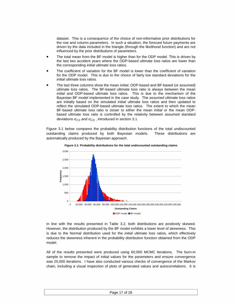
Figure 3.1 below compares the probability distribution functions of the total undiscounted outstanding claims produced by both Bayesian models. These distributions are automatically produced by the Bayesian approach.

Figure 3.1: Probability distributions for the total undiscounted outstanding claims

0

500

1,000

1,500

2,000

2,500

3,000

0 20,000 40,000 60,000 80,000 100,000 120,000 140,000 160,000 180,000 200,000 220,000 240,000

Outstanding Claims

Fre

qu

ency

ODP model BF model

In line with the results presented in Table 3.2, both distributions are positively skewed. However, the distribution produced by the BF model exhibits a lower level of skewness. This is due to the Normal distribution used for the initial ultimate loss ratios, which effectively reduces the skewness inherent in the probability distribution function obtained from the ODP model. All of the results presented were produced using 60,000 MCMC iterations. The burn-in sample to remove the impact of initial values for the parameters and ensure convergence was 25,000 iterations. I have also conducted various checks of convergence of the Markov chain, including a visual inspection of plots of generated values and autocorrelations. It is

of 26

worth noting that these and other tests are readily available through WinBUGS as part of the standard modelling output. The presented results were based on a particular specification of the two Bayesian models. It is however possible to make some further modifications to these models, including the introduction of informative prior distributions for the row and column parameters in the ODP model or changing standard deviations σ(1)i and σ(2)i in the BF model. More significant changes could also include:

• Introduction of a distribution for the over-dispersion parameter in the ODP model

• Choice of a non-normal distribution for the initial ultimate loss ratio in the BF model

• Choice of other than Gamma distributions for the row and column parameters in the ODP model


of 26

4. Summary and conclusions

The main purpose of this paper is to provide a high-level overview of the theory underlying the Bayesian approaches and to show how they could be applied in the context of stochastic reserving. In particular, the theoretical discussion is supported by a case study where two statistical models (underlying the chain ladder and Bornhuetter-Fergusson methods) have been implemented using Bayesian approaches. I acknowledge that these models have a number of limitations as highlighted by other researchers. In particular, the ODP model is not generally appropriate for data with negative incremental amounts (e.g. incurred cost data), while the Normal distribution assumed for the initial ultimate loss ratios in the BF model may not be suitable, given the positive skewness inherent in loss distributions observed in general insurance. It is however important to note that the presented models are fairly simple to apply and in my opinion quite adequate for illustration purposes in this paper. In practice, it may be more appropriate to incorporate modifications mentioned in sections 3.1 and 3.3 or to use a completely different Bayesian model. My experience is that Bayesian methods are not commonly used in stochastic reserving in Australia. I hope that this paper has highlighted some of the key benefits of these approaches and will encourage Australian actuaries to include these methods in their stochastic reserving toolkit. As noted in previous sections, I have included the WinBUGS code used for the case study in the Appendix. I would encourage practitioners to download a free copy of WinBUGS and experiment with this code. I have also included a comprehensive bibliography on Bayesian stochastic reserving for readers interested in further research, including some papers on the applications of WinBUGS in actuarial science. One of the key benefits of Bayesian stochastic reserving is its flexibility and, in particular, capability to incorporate actuarial judgement and external information into the stochastic reserving process. The case study also illustrated how a Bayesian BF model could be used to incorporate actuarial judgement/external information. In particular, my specification of this model led to a dramatic decrease in the volatility of simulated undiscounted outstanding claims compared to the results from the ODP model. Having said that, I believe that there is still more research required in the context of the implementation of actuarial judgement and external information into Bayesian stochastic reserving process.


of 26

5. Acknowledgements

I would like to express my gratitude and appreciation to the peer-reviewers of this paper Karl Marshall and Peter England. They have both provided valuable peer-review feedback and general support in writing this paper. I also would like to thank my employer, Quantium, for the support provided in writing this paper. Whilst, as the author, I have made every effort to provide accurate and current information I do not warrant that the information contained herein is in every respect accurate and complete. I expressly disclaim any responsibility for any errors or omissions or for any reliance placed on this paper. If you have any comments on or queries about the paper, please feel free to email me at: [email protected]


of 26

6. Appendix

This section presents WinBUGS code used in the case study. This code is based on the material previously presented by Verrall[23] and Scollnik[22]. There are several aspects of the existing code where further model extensions could be incorporated including:

• Replacing the ODP distribution with a Gamma distribution for future observations, so that forecast incremental payments look more realistic

• Incorporation of a full Bayesian approach for the over-dispersion parameter, as described by Sollnik in Antonio, Beirlant and Hoedemakers [1]

• Changes to the weight parameter and the distribution for initial and assumed ultimate loss ratios

• Choice of different prior distributions for the row and column parameters in the ODP model

It is important to note that if a different data set is used with the code below the following inputs will need to be changed or adjusted:

• Parameters a[1] and phi (England and Verrall [10] show formulas how phi can be estimated from the data)

• Scale and shape parameters of the Gamma prior distributions for parameters a and p1

• Initial values for a and p1 model { # ODP model for data: # x are row parameters # y are column parameters # phi is the over-dispersion or scale parameter and it is a plug-in estimate in the code below for( i in 1 : 55 ) { Z[i] <- C[i]/1000 log(mu[i]) <- x[row[i]] + y[col[i]] # Zeros trick to cope with non-positive integer data: zeros[i] <- 0 zeros[i] ~ dpois(PoissMean[i]) PoissMean[i] <- (mu[i] - Z[i]*log(mu[i]) + loggam(Z[i] + 1))/phi # MINUS log likelihood } # ODP model for future observations: for( i in 56 : 100 ) { mu2[i] <- mu[i]/phi C[i] ~ dpois(mu2[i]); log(mu[i]) <- x[row[i]] + y[col[i]] Z[i] <- phi*C[i] } for( i in 1 : 100 ) { fit[i] <- Z[i]*1000 } phi <- 1.08676 # as per Verrall [23] a[1] <- 18.834 # set equal to the incremental payment in the latest development year of the first accident year x[1] <- log(a[1])

of 26

# Prior distributions for row parameters: for (k in 2:10) { a[k] ~ dgamma(0.000001,0.0000001) x[k] <- log(a[k]) } # Prior distributions for column parameters: # p1 are intermediate parameters to derive incremental paid developments # p are incremental payout ratios for (k in 1:10) { p1[k] ~ dgamma(0.00001,0.0001) } s <- sum(p1[1:10]) for (k in 1:10) { p[k] <- p1[k]/s y[k] <- log(p[k]) } #Chain ladder factors required for the BF method # pc are cumulative payout ratios # CLfact are chain ladder factors # CumCLfact are cumulative chain ladder factors pc[1] <- p[1] for (k in 2:10) {pc[k] <- pc[k-1] + p[k]} for (k in 1:9) {CLFact[k] <- pc[k+1]/pc[k]} for (j in 1:9) { for (i in 1:10) {CLFactByAccYr[i,j] <- CLFact[j]} } for( i in 1 : 10 ) { for( j in 1 : 9 ) {CumCLfact[ i, j ] <- prod(CLFactByAccYr[ i, j : 9 ] )} } #Chain ladder ODP outstanding claims by accident year and in total: CLOS[1] <- 0 CLOS[2] <- fit[56] CLOS[3] <- sum(fit[57:58]) CLOS[4] <- sum(fit[59:61]) CLOS[5] <- sum(fit[62:65]) CLOS[6] <- sum(fit[66:70]) CLOS[7] <- sum(fit[71:76]) CLOS[8] <- sum(fit[77:83]) CLOS[9] <- sum(fit[84:91]) CLOS[10] <- sum(fit[92:100]) CLTotalOS <- sum(CLOS[2:10]) #BF model for future observations: # lossratio[ i, 1 ] are initial ultimate loss ratios # lossratio[ i, 2 ] are ODP ultimate loss ratios # lossratio[ i, 3 ] are intermediate step to achieve assumed loss ratios;

# note that the aim is actually to obtain # lossratio[ i, 3 ] ~ dnorm( lossratio[ i, 1 ], weight*tauLR [ i ] ); however this is not possible and # the zeros trick needs to be applied instead

# weight is a parameter that specifies how much weight is given to the initial ultimate loss ratio, # the lower it is the less weight is given to the ODP ultimate loss ratio

weight <- 1 for( i in 1 : 10 ) { lossratio[ i, 1 ] ~ dnorm( meanLR[ i ], tauLR [ i ] ) tauLR [ i ] <- 1 / pow(stdLR [ i ], 2) lossratio[ i, 2 ] <- (sum( CLOS[ i ] )+paidTodate [ i ]) / premium[ i ]

of 26

lossratio[ i, 3 ] <- cut( lossratio[ i, 2 ] ) # Use the zeros trick code below in place of line above in order to avoid defining # the lossratio[ i, 3 ] node twice.

zero[ i ] <- 0 zero[ i ] ~ dpois( phi2[ i ] ) phi2[ i ] <- weight * tauLR[ i ] * ( lossratio[ i, 3 ] - lossratio[ i, 1 ] ) *

( lossratio[ i, 3 ] - lossratio[ i, 1 ] ) * 0.5 ultimate[ i ] <- premium[ i ] * lossratio[ i, 1 ] } for( i in 1 : 10 ) { BFY[ i, 1 ] <- ultimate[ i ] * 1/CumCLfact[ i, 1 ] for( j in 2 : 9 ) {BFY[ i, j ] <- ultimate[ i ] * ( 1/CumCLfact[ i, j ] - 1/CumCLfact[ i, j - 1 ] )} BFY[ i, 10 ] <- ultimate[ i ] * ( 1 - 1/CumCLfact[ i, 9 ] ) } #BF outstanding claims by accident year and in total: BFOS[1] <- 0 for( i in 2 : 10 ) {BFOS[ i ] <- sum( BFY[ i, 10 + 2 - i : 10 ] )} BFTotalOS <- sum(BFOS[1:10]) } # DATA list( row = c(1,1,1,1,1,1,1,1,1,1, 2,2,2,2,2,2,2,2,2, 3,3,3,3,3,3,3,3, 4,4,4,4,4,4,4, 5,5,5,5,5,5, 6,6,6,6,6, 7,7,7,7, 8,8,8, 9,9, 10, 2, 3,3, 4,4,4, 5,5,5,5, 6,6,6,6,6, 7,7,7,7,7,7, 8,8,8,8,8,8,8, 9,9,9,9,9,9,9,9, 10,10,10,10,10,10,10,10,10), col = c(1,2,3,4,5,6,7,8,9,10, 1,2,3,4,5,6,7,8,9, 1,2,3,4,5,6,7,8, 1,2,3,4,5,6,7, 1,2,3,4,5,6, 1,2,3,4,5, 1,2,3,4, 1,2,3, 1,2, 1, 10, 9,10, 8,9,10, 7,8,9,10, 6,7,8,9,10, 5,6,7,8,9,10, 4,5,6,7,8,9,10, 3,4,5,6,7,8,9,10, 2,3,4,5,6,7,8,9,10), C = c(5012,3257,2638,898,1734,2642,1828,599,54,172, 106,4179,1111,5270,3116,1817,-103,673,535, 3410,5582,4881,2268,2594,3479,649,603, 5655,5900,4211,5500,2159,2658,984, 1092,8473,6271,6333,3786,225, 1513,4932,5257,1233,2917,

of 26

557,3463,6926,1368, 1351,5596,6165, 3133,2262, 2063, NA, NA,NA, NA,NA,NA, NA,NA,NA,NA, NA,NA,NA,NA,NA, NA,NA,NA,NA,NA,NA, NA,NA,NA,NA,NA,NA,NA, NA,NA,NA,NA,NA,NA,NA,NA, NA,NA,NA,NA,NA,NA,NA,NA,NA), paidTodate=c(18834,16704,23466,27067,26180,15852,12314,13112,5395,2063), premium=c(28975,20478,28984,38432,47290,24308,23228,30721,29611,29407), meanLR=c(0.71,0.71,0.71,0.71,0.71,0.71,0.71,0.71,0.71,0.71), stdLR=c(0.071,0.071,0.071,0.071,0.071,0.071,0.071,0.071,0.071,0.071)) # INITIAL VALUES

# Note that for the loss ratios in the BF model, the initial values need to be generated within WinBUGS. # Alternatively they could be add here as another vector

list( a = c(NA,20,20,20,20,20,20,20,20,20), p1 = c(0.1,0.1,0.1,0.1,0.1,0.1,0.1,0.1,0.1,0.1 ), C = c(NA,NA,NA,NA,NA,NA,NA,NA,NA,NA, NA,NA,NA,NA,NA,NA,NA,NA,NA, NA,NA,NA,NA,NA,NA,NA,NA, NA,NA,NA,NA,NA,NA,NA, NA,NA,NA,NA,NA,NA, NA,NA,NA,NA,NA, NA,NA,NA,NA, NA,NA,NA, NA,NA, NA, 0, 0,0, 0,0,0, 0,0,0,0, 0,0,0,0,0, 0,0,0,0,0,0, 0,0,0,0,0,0,0, 0,0,0,0,0,0,0,0,

0,0,0,0,0,0,0,0,0))


of 26

7. Bibliography

1. Antonio, K. , J. Beirlant and T. Hoedemakers (2005): “Discussion of papers already

published: ‘‘A Bayesian Generalized Linear Model for the Bornhuetter-Ferguson Method of Claims Reserving,’’ R. J. Verrall, July 2004”. North American Actuarial Journal. Available from: http://www.soa.org/library/journals/north-american-actuarial-journal/2005/july/naaj0503-8.pdf

2. Berger, J. O. (1985): “Statistical Decision Theory and Bayesian Analysis”. 2nd edition New York, Springer-Verlag

3. Bernardo, J. M. and A. F. M. Smith (1994): “Bayesian Theory”. New York, John Wiley & Sons

4. Bornhuetter, R. L. and R. E. Ferguson (1972): “The Actuary and IBNR”. Proceedings of the Casualty Actuarial Society 59: pages 181–95

5. Carlin B. P. and T. A. Louis (2000): “Bayes and Empirical Bayes Methods for Data Analysis: texts in statistical science”. 2nd edition, Chapman and Hall/CRC

6. de Alba, E. (2002): “Bayesian Estimation of Outstanding Claim Reserves,” North American Actuarial Journal 6 (4): pages 1-20

7. Dellaportas, P. and A. F. M. Smith (1993): “Bayesian inference for generalized linear and proportional hazards models via Gibbs sampling”. Applied Statistics, 42(3): pages 443-459

8. England, P. D. (2002): “Bayesian Stochastic Reserving: Background Statistics”. EMB presentation

9. England, P. D. and R. J. Verrall (2002): “Stochastic claims reserving in general insurance”. Institute of Actuaries and Faculty of Actuaries. Available from http://www.actuaries.org.uk/__data/assets/pdf_file/0014/31721/sm0201.pdf

10. England, P. D. and R. J. Verrall (2006): “Predictive distributions of outstanding claims in general insurance”. Annals of Actuarial Science, 1, II: pages 221-270

11. Geman, S. and D. Geman (1984): “Stochastic relaxation, Gibbs distribution and Bayesian restoration of images”. IEE Transactions on Pattern Analysis and Machine Intelligence 6: pages 721–741

12. Gelfand, A. E. and A. F. M. Smith (1990): “Sampling-based approaches to calculating marginal densities”. J. Am. Stat. Asso. 85: pages 398–409

13. Gilks, W. R. and P. Wild (1992): “Adaptive rejection sampling for Gibbs sampling”. Applied Statistics, 41(2): pages 337-348

14. Gilks, W. R., Best N. G. and K. K. C. Tan (1994): “Adaptive Rejection Metropolis Sampling within Gibbs Sampling”. Applied Statistics 44: pages 455–472

15. Historical Loss Development Study (1991). Reinsurance Association of America. Washington D.C.

16. Igloo Professional with ExtrEMB (2007). Igloo Professional with ExtrEMB v3.1.7. EMB Software Ltd, Epsom, U.K.

17. Ntzoufras, I. and P. Dellaportas (2002): “Bayesian modelling of outstanding liabilities incorporating claim count uncertainty”. North American Actuarial Journal, 6(1): pages 113-136

18. O’Dowd C., Smith A. and P. Hardy (2005): “A Framework for Estimating Uncertainty in Insurance Claims Cost”. Proceedings of the 15th General Insurance Seminar

19. Renshaw, A. E. and R. J. Verrall (1998): “A Stochastic Model Underlying the Chain Ladder Technique,” British Actuarial Journal 4(4): pages 903–23

of 26

20. Risk Margins Taskforce (2008): “A Framework for Assessing Risk Margins”. Institute of Actuaries Australia, 16th General Insurance Seminar

21. Scollnik, D. P. M. (2001): “Actuarial modelling with MCMC and BUGS”. North American Actuarial Journal, 5(2): pages 96-125

22. Scollnik, D.P.M. (2004): “Bayesian Reserving Models Inspired by Chain Ladder Methods and Implemented Using WinBUGS”. Available from: http://www.soa.org/library/proceedings/arch/2004/arch04v38n2_3.pdf

23. Verrall, R. J. (2004): “A Bayesian generalized linear model for the Bornhuetter-Ferguson method of claims reserving”. North American Actuarial Journal, 8(3)

24. Verrall, R. J. and P. D. England (2005): “Incorporating expert opinion into a stochastic model for the chain-ladder technique”. Insurance: Mathematics and Economics 37: pages 355–370

25. Walsh, B. (2004): “Markov Chain Monte Carlo and Gibbs Sampling”. Lecture Notes, Department of Statistics at Columbia University. Available from: http://www.stat.columbia.edu/~liam/teaching/neurostat-spr07/papers/mcmc/mcmc-gibbs-intro.pdf

stochastic reserving – case study using a bayesian … · stochastic reserving – case study...

Documents