stochastic reserving methods - actuaries institute · stochastic reserving methods advantages,...

Stochastic Reserving Methods

Advantages, Disadvantages, Key Issues and Lessons Learnt

byAndrew Smith & Mitchell Prevett

Agenda

1. Introduction

2. Case study

3. Summary

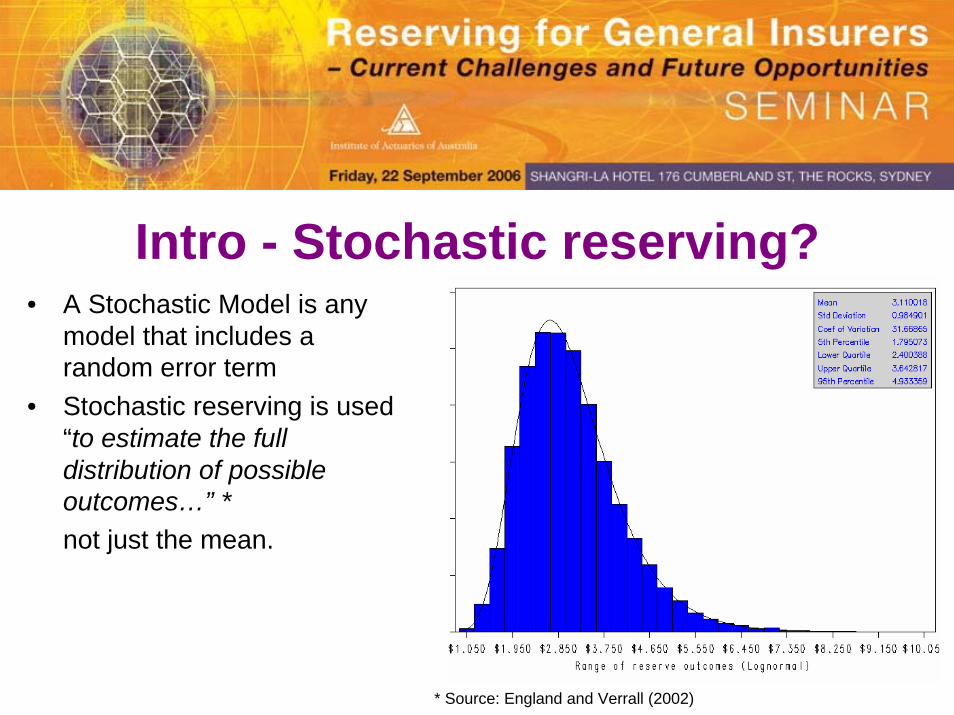
Intro - Stochastic reserving?• A Stochastic Model is any

model that includes a random error term

• Stochastic reserving is used “to estimate the full distribution of possible outcomes…” *not just the mean.

* Source: England and Verrall (2002)

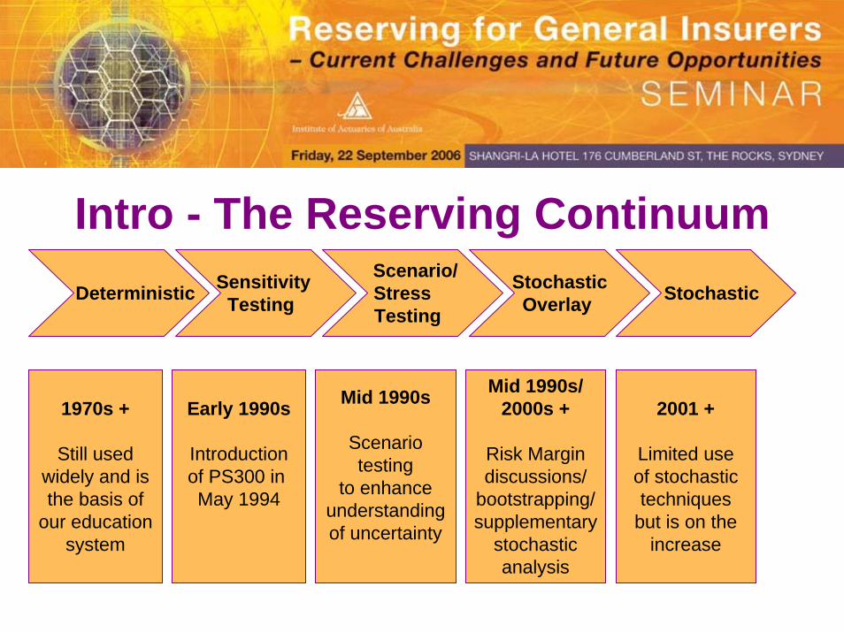
Intro - The Reserving ContinuumDeterministic Sensitivity

Testing

Scenario/StressTesting

StochasticOverlay Stochastic

1970s +

Still usedwidely and isthe basis of

our educationsystem

Early 1990s

Introductionof PS300 in May 1994

Mid 1990s

Scenariotesting

to enhanceunderstandingof uncertainty

Mid 1990s/2000s +

Risk Margindiscussions/

bootstrapping/supplementary

stochasticanalysis

2001 +

Limited useof stochastictechniques

but is on theincrease

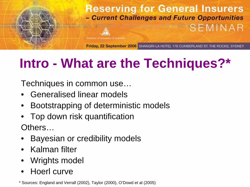
Intro - What are the Techniques?*Techniques in common use…• Generalised linear models• Bootstrapping of deterministic models• Top down risk quantificationOthers…• Bayesian or credibility models• Kalman filter• Wrights model• Hoerl curve

* Sources: England and Verrall (2002), Taylor (2000), O’Dowd et al (2005)

Case study – Weekly Comp PPAC GLMWhat?

Weekly compensation for a large accident compensation schemeWhy?

1. Superimposed inflation? Is it evident? What is the level?2. Better understand the uncertainties in the reserving?3. What insights can we derive to build into the main valuation?4. Estimation of risk margins

How?

E(Pmtsi,j) = Activesi,j-1 x E(ContRatej) x E(PPACj), where i = devqtr, j = accqtr

GLM1 – ContRatei,j = Activesi,j / Activesi,j-1 = f(i, j, i+j) + error

GLM2 – PPACi,j = Pmtsi,j / Activesi,j = f(i, j, i+j) + error

Fitted GLM• Short, medium and

long term rates are modelled separately

• Over-dispersed Poisson / Log GLM on Activei,j

• Offset - Log(Activei,j-1)• Binary and linear

segment transforms are used

Model Parameter Estimates - Short TermModel Predictor Formula Estimate Multiple

Intercept 0.0000Development Quarter = 1 (devqtr = 1) -0.1154 89%Development Quarter = 2 (devqtr = 2) -1.1367 32%Development Quarter = 3 (devqtr = 3) -0.4618 63%Development Quarter (linear 4 to 7) min(max(devqtr-4,0),7-4) 0.0498 105%Development Quarter (linear 11 to 15) min(max(devqtr-11,0),15-11) 0.0089 101%Development Quarter (linear from 15) max(devqtr-15,0) 0.0012 100%Development Quarter (greater than 3) (devqtr ge 4) -0.2958 74%Experience Quarter (step to 30 June XX) (expqtrdate lt '30junXX'd) 0.0233 102%(Development Quarter = 1) and Exp Qtr (prior to 30 June XX) 0.2132 124%(Development Quarter = 2) and Exp Qtr (prior to 30 June XX) -0.0708 93%

Model Parameter Estimates - Medium TermModel Predictor Formula Estimate Multiple

Intercept -0.0264Development Quarter (after 44) (devqtr ge 44) 0.0128 101%

Continuance rates GLM PPAC GLM Superimposed inflation

Full reserve distribution

GLM vs. Deterministic Model

1 4 7 10 13 16 19 22 25 28 31 34 37 40 43 46 49Development Quarter

Con

tinua

nce

Rat

e %

GLM GLM Low er Bound GLM Upper Bound Deterministic Model

Comparison to deterministic model

• GLM fitted rates compare well with the deterministic fitted rates

• Confidence limits can be calculated for the GLM fitted function (this assumes no correlations in estimates)

Confidence limits indicate more certainty parameter estimates

Greater uncertainty in parameter estimates



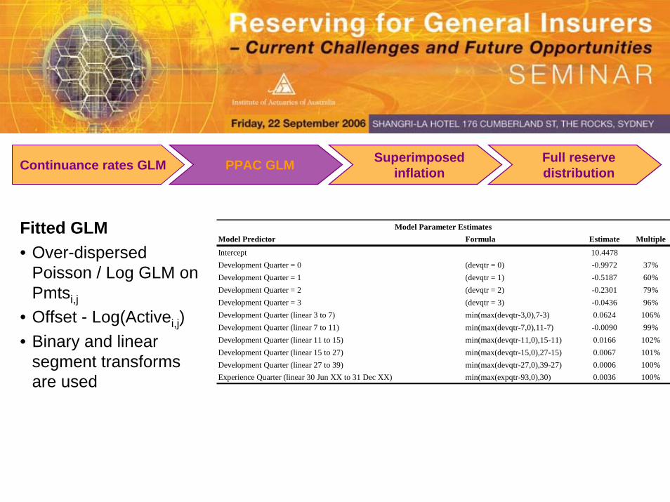
Fitted GLM• Over-dispersed

Poisson / Log GLM on Pmtsi,j

• Offset - Log(Activei,j)• Binary and linear

segment transforms are used

Model Parameter Estimates Model Predictor Formula Estimate Multiple

Intercept 10.4478Development Quarter = 0 (devqtr = 0) -0.9972 37%Development Quarter = 1 (devqtr = 1) -0.5187 60%Development Quarter = 2 (devqtr = 2) -0.2301 79%Development Quarter = 3 (devqtr = 3) -0.0436 96%Development Quarter (linear 3 to 7) min(max(devqtr-3,0),7-3) 0.0624 106%Development Quarter (linear 7 to 11) min(max(devqtr-7,0),11-7) -0.0090 99%Development Quarter (linear 11 to 15) min(max(devqtr-11,0),15-11) 0.0166 102%Development Quarter (linear 15 to 27) min(max(devqtr-15,0),27-15) 0.0067 101%Development Quarter (linear 27 to 39) min(max(devqtr-27,0),39-27) 0.0006 100%Experience Quarter (linear 30 Jun XX to 31 Dec XX) min(max(expqtr-93,0),30) 0.0036 100%



GLM vs. Deterministic Model

1 5 9 13 17 21 25 29 33 37 41 45 49Development Quarter

Paym

ents

Per

Act

ive

Cla

im (P

PAC

) $'s

GLM GLM Low er Bound GLM Upper Bound Deterministic Model

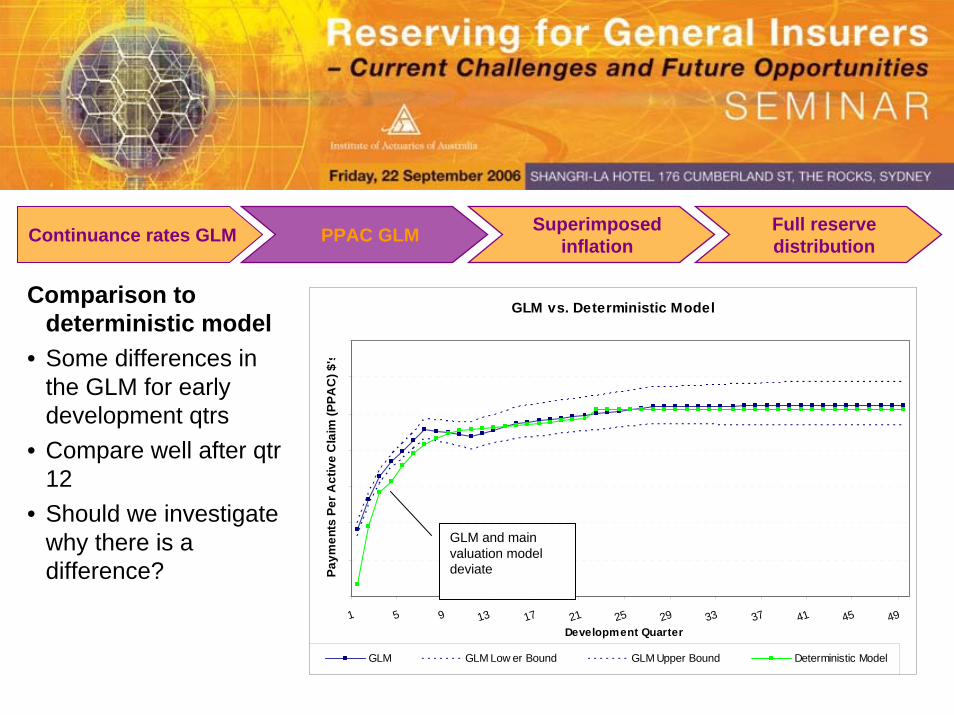
GLM and main valuation model deviate

Comparison to deterministic model

• Some differences in the GLM for early development qtrs

• Compare well after qtr 12

• Should we investigate why there is a difference?



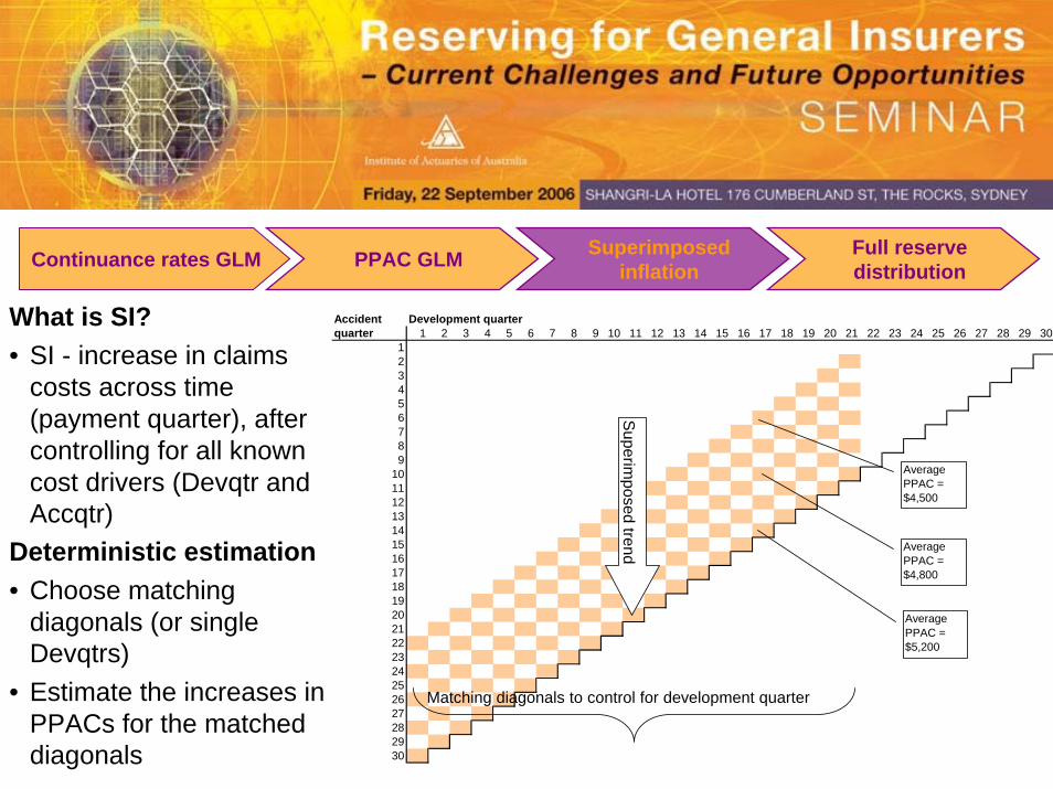
What is SI?• SI - increase in claims

costs across time (payment quarter), after controlling for all known cost drivers (Devqtr and Accqtr)

Deterministic estimation• Choose matching

diagonals (or single Devqtrs)

• Estimate the increases in PPACs for the matched diagonals



Accident Development quarterquarter 1 2 3 4 5 6 7 8 9 10 11 12 13 14 15 16 17 18 19 20 21 22 23 24 25 26 27 28 29 30

123456789

101112131415161718192021222324252627282930

Superim

posed trend

Matching diagonals to control for development quarter

Average PPAC = $5,200



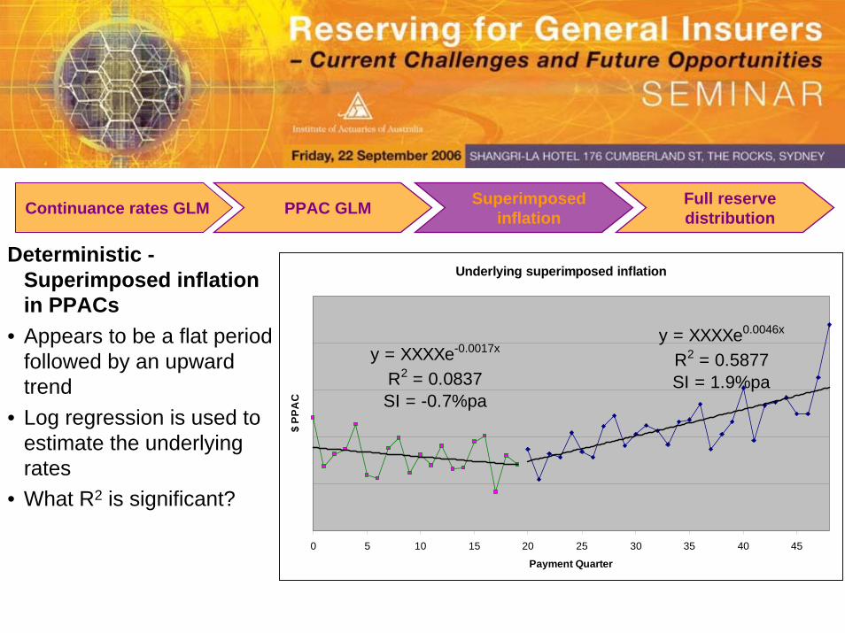
Deterministic -Superimposed inflation in PPACs

• Appears to be a flat period followed by an upward trend

• Log regression is used to estimate the underlying rates

• What R2 is significant?

Underlying superimposed inflation

y = XXXXe0.0046x

R2 = 0.5877SI = 1.9%pa

y = XXXXe-0.0017x

R2 = 0.0837SI = -0.7%pa

0 5 10 15 20 25 30 35 40 45

Payment Quarter

$ PP

AC



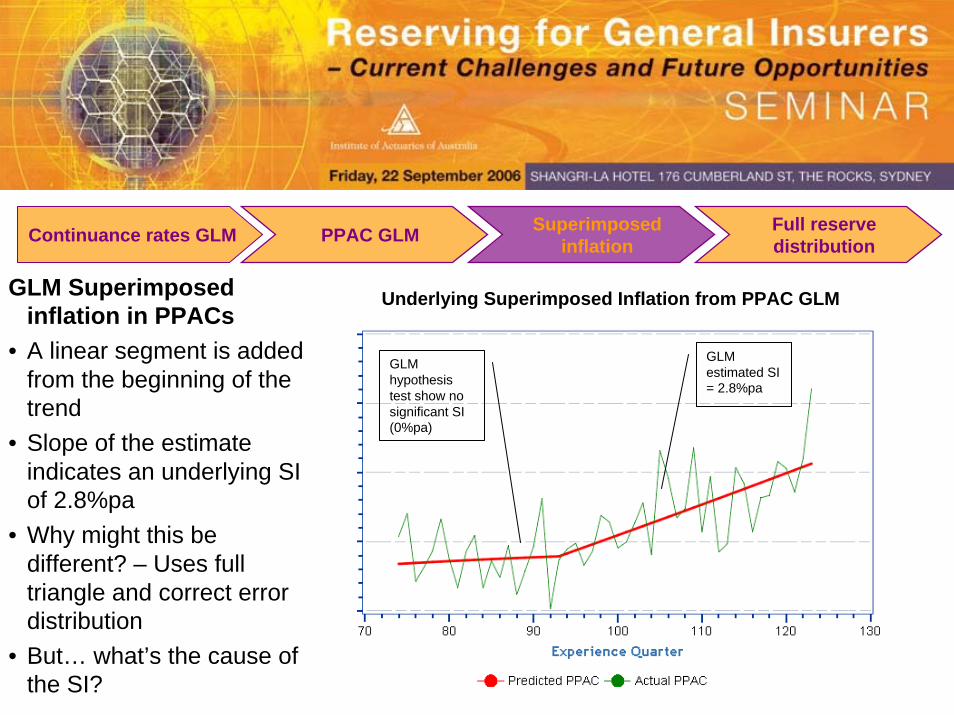
GLM estimated SI = 2.8%pa

GLM hypothesis test show no significant SI (0%pa)

GLM Superimposed inflation in PPACs

• A linear segment is added from the beginning of the trend

• Slope of the estimate indicates an underlying SI of 2.8%pa

• Why might this be different? – Uses full triangle and correct error distribution

• But… what’s the cause of the SI?

Underlying Superimposed Inflation from PPAC GLM



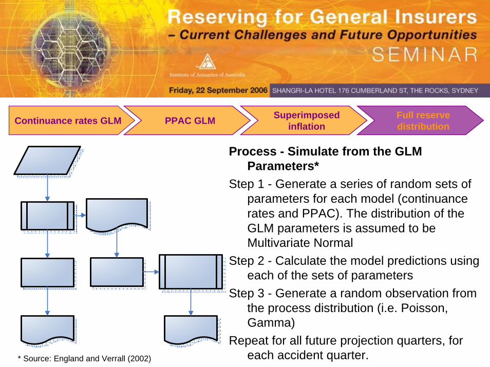
Process - Simulate from the GLM Parameters*

Step 1 - Generate a series of random sets of parameters for each model (continuance rates and PPAC). The distribution of the GLM parameters is assumed to be Multivariate Normal

Step 2 - Calculate the model predictions using each of the sets of parameters

Step 3 - Generate a random observation from the process distribution (i.e. Poisson, Gamma)

Repeat for all future projection quarters, for each accident quarter.



* Source: England and Verrall (2002)



Simulation of Active Claim Numbers

• A selected accident quarter’s projections are shown

• 5 simulations are displayed as well as the mean and 5th and 95th

percentiles• GLM simulated mean

compares well with the valuation for this accident period



Simulation of Active Claim Numbers and PPACs

• Simulated cash flows are projected for the liability as at the valuation date

• The mean and 5th and 95th

percentiles are calculated to show the implied the uncertainty

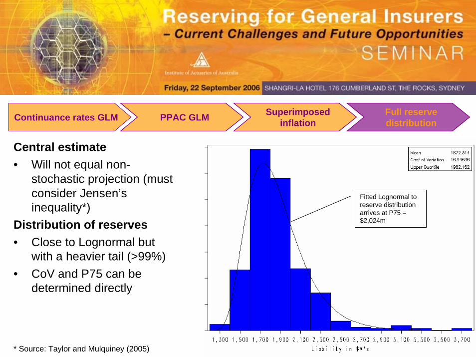
Central estimate• Will not equal non-

stochastic projection (must consider Jensen’s inequality*)

Distribution of reserves• Close to Lognormal but

with a heavier tail (>99%)• CoV and P75 can be

determined directly

Fitted Lognormal to reserve distribution arrives at P75 = $2,024m



* Source: Taylor and Mulquiney (2005)

Advantages of Stochastic Reserving1. Superimposed inflation and trends – statistical significance

can be used to determine if trends are “real”.2. Hypothesis testing – impact of legislative changes, benefit

changes, or any other claims administration changes3. Downside risk - through estimation of full distribution the

downside risk and hence risk margins can be estimated4. Individual claims modelling – stochastic models are suitable

for individual claims modelling5. Model update (control cycle) – testing recent experience

against the model we can determine if it needs to be updated

Disadvantages of Stochastic Reserving

1. Less transparent – can be harder to explain to management2. Reliable data – generally more reliable data is required to

construct a more sophisticated model3. Incorporating judgement – more complex to overlay

judgment based adjustments4. Costly and time consuming – can be difficult to articulate the

value5. Seen as the fix all - If traditional methods fail then SR is

unlikely to succeed…it’s not an automatic fix6. Model variability NOT risk – the past may not be a guide to

the future

Risk FrameworkEmpirical estimation of the claims distribution….• Workshop the key risk drivers• Use qualitative and quantitative methods to assess the range of

scenarios / outcomes due to a given risk driver.• Risk assessment phase likely to include stochastic analysis• Determine a distribution for each risk driver• Use stochastic simulation to combine the major sources of

uncertainty

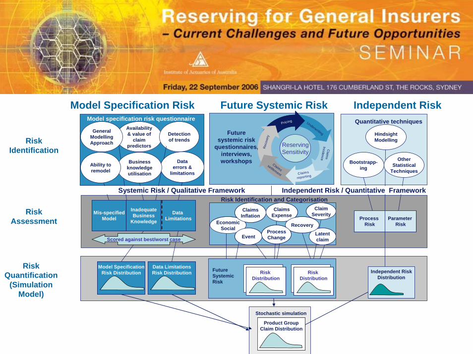
Model Specification Risk Future Systemic Risk Independent Risk

Risk Quantification

(SimulationModel)

RiskAssessment

RiskIdentification

Availability & value of

claim predictors

Detection of trends

Stochastic simulation

Data errors &

limitations

Model specification risk questionnaire

Future systemic risk

questionnaires, interviews, workshops

Quantitative techniques

Other Statistical

Techniques

Bootstrapp-ing

Independent RiskDistribution

Mis-specifiedModel

Data Limitations

InadequateBusiness

Knowledge

Mis-specifiedModel

Data Limitations

InadequateBusiness

Knowledge Parameter Risk

Process Risk

Parameter Risk

Process Risk

Risk Identification and Categorisation

Model SpecificationRisk Distribution

Model SpecificationRisk Distribution

Product GroupClaim Distribution

Product GroupClaim Distribution

Future Systemic Risk

Risk DistributionRisk

Distribution


DistributionRisk

Distribution

Data LimitationsRisk DistributionData LimitationsRisk Distribution

Scored against best/worst case

General Modelling Approach

Business knowledge utilisation

Ability to remodel

Hindsight Modelling

Systemic Risk / Qualitative Framework Independent Risk / Quantitative Framework

Latent claim

Economic Social

Claims Inflation

Claims Expense

Event

Claim Severity

RecoveryProcess Change

Latent claim

Economic Social

Claims Inflation

Claims Expense

Event

Claim Severity

RecoveryProcess Change


Distribution


DistributionRisk

Distribution

Pricing Underwriting

Claim

s Incidence

Claims

reporting

Claims settlement

Rec

over

y

ReservingSensitivity

Pricing Underwriting

Claim

s Incidence

Claims

reporting

Claims settlement

Rec

over

y

ReservingSensitivity

Summary• Stochastic techniques are continuing to gain favour –

part of tool suite

• They are not the magic answer but an important supplement / extension to current reserving practices

• Quantitative assessments should be combined with qualitative assessments to capture all aspects of risk

• Taylor G and Mulquiney P (2005). Modelling mortgage insurance as a multi-state process. UNSW Actuarial Studies Research Symposium

• England P and Verrall R (2002). Stochastic Claims Reserving in General Insurance. Presented to the Institute of Actuaries 28 Jan 02

• Taylor G (2000). Loss Reserving: An Actuarial Perspective. Kluwer Academic Publishers

• O’Dowd C, Smith A and Hardy P (2005). A Framework for Estimating Uncertainty in Insurance Claims Cost. Presented to XVth General Insurance Seminar.

References

Stochastic Reserving Methods

Advantages, Disadvantages, Key Issues and Lessons Learnt

byAndrew Smith & Mitchell Prevett

stochastic reserving methods - actuaries institute · stochastic reserving methods advantages,...

Documents