stochastic simulation with generative adversarial networks€¦ · conditioning of generative...
TRANSCRIPT
Stochastic Simulation with
Generative Adversarial Networks
Lukas Mosser, Olivier Dubrule, Martin J. Blunt

● Task: Draw (new) samples from unknown density given a set of samples
● Generative Adversarial Networks (GAN)○ Two competing Neural Networks
● Variational Autoencoders (VAE)○ Bayesian Graphical Model of data distribution
● Autoregression (Pixel-CNN)○ Conditional Distribution on every sample
○ Many More ...
(Deep) Generative Methods
1
Training Set
Generative
Model
Latent
Variables
Samples from Model
Main Problem: How to find the generative model?

(Goodfellow et. al. 2014)
𝑝𝑑𝑎𝑡𝑎 𝑥
Latent space z
Generator (z)Training Data 𝑥
Discriminator(x)
?
Gradient-based
Feedback
Noise prior
Generative Adversarial Networks – Toy Example
2

• Requirements:
• Training Set of data
• Generator – creates samples G(z)
• Discriminator – evaluates samples
• Cost function:
• GAN training – two step procedure in supervised way
• Discriminator training step – Generator fixed
• Train on real data samples
• Train on fake samples
• Generator training step – Discriminator fixed
• Push generator towards “real” images
Generative Adversarial Networks – Training
3

• Oolitic Limestone
• Intergranular pores
• Intragranular Micro-Porosity
• Ellipsoidal grains
• 99% Calcite
• Image Size:
- 𝟗𝟎𝟎^𝟑 voxels @ 26.7 𝝁𝒎
Extract Non-Overlapping
Training Images (𝟔𝟒𝟑 𝒗𝒐𝒙𝒆𝒍𝒔)
Training Set
Ketton Limestone Dataset and Preprocessing
5
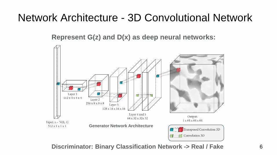
Discriminator: Binary Classification Network -> Real / Fake
Generator Network Architecture
Represent G(z) and D(x) as deep neural networks:
Network Architecture - 3D Convolutional Network
6

Intergranular Porosity
Moldic Features
Micro-Porosity
Training Time: 8 hours
Generation: 5 sec.
High visual quality
Needs quantitative measures
Reconstruction Quality – Unconditional Simulation
Ketton Training Image GAN generated sample
7

Statistical Properties
• Two-Point Probability Function 𝑺𝟐 𝒓
» Radial Average / Directional
Minkowski Functionals
• Porosity 𝝓
• Specific Surface Area 𝑺𝒗• Integral of Mean Curvature
• Specific Euler Characteristic 𝝌𝒗• Compute as function of image gray-level
=> Characteristic Curves
Flow Properties: Solve Stokes flow in pore domain
• Permeability + Velocity Distributions
Reconstruction Quality Criteria
8
3

Isotropic Covariance
Pronounced Oscillations -> “Hole-Effect”
• Captured by GAN model
Smaller Variance of GAN model
Ketton Comparison – Directional 𝑺𝟐 𝒓
9

Isotropic Permeability
Range of effective (flowing) porosity: Data (0.29- 0.37) GAN (0.31-0.33)
Same order of magnitude and ന𝒌 − 𝝓 relationship
Ketton Comparison – Permeability
10

Smaller Variance in GAN generated samples: Why?
𝑝𝑑𝑎𝑡𝑎 𝑥Latent space z
𝑝𝑔𝑒𝑛 𝑥
Generator can miss modes of the data distribution -> Mode-Collapse
What does the Generator learn?
Multi-scale Representation of pore space
Opening the GAN black box
11

Latent space z
Interpolation in latent space:
Shows that generator has
learned a meaningful representation in a
lower dimensional space!
Interpolation path visualization
Latent Space Interpolation
𝑧∗ = 𝛽 𝑧𝑠𝑡𝑎𝑟𝑡 + 1 − 𝛽 𝑧𝑒𝑛𝑑 , 𝛽 ∈ [0, 1]
12

Computational Effort
Main Computation cost training:
Amortizes with number of samples due to low per sample cost / runtime13

Image Inpainting (Yeh et al. 2016)
(Cat, Dog, Leopard, Dachshund)
Credit: Kyle Kastner𝑴 ∙ 𝒙 Human Artist 𝑳𝟐 𝑳𝒐𝒔𝒔 𝑳𝒄𝒐𝒏𝒕𝒆𝒏𝒕 + 𝑳𝒑𝒆𝒓𝒄
Optimize loss by gradient descent on latent vector z
15
Task: Restore missing details given a corrupted / masked image 𝑴 ∙ 𝒙
Use a generative model G(z) to find missing details, conditional to given information.
Contextual Loss: 𝑳𝒄𝒐𝒏𝒕𝒆𝒏𝒕 = 𝝀 𝑴 ∙ 𝑮 𝒛 −𝑴 ∙ 𝒙𝟐
Perceptual Loss: 𝑳𝒑𝒆𝒓𝒄 = 𝒍𝒐𝒈(𝟏 − 𝑫(𝑮 𝒛 )
Corresponds to likelihood
Regularization for prior
Stay close to “real” images

Conditioning – Pore Scale Example
Two-dimensional data at pore-scale more abundant e.g. thin-sections
Combine 3D generative model G(z) with 2D conditioning data
Generative Model: Ketton Limestone GAN (Part 1)
Mask: Three orthogonal cross-sections, honor 2D data in a 3D image
Contextual Loss: 𝑳𝒄𝒐𝒏𝒕𝒆𝒏𝒕 = 𝝀 𝑴 ∙ 𝑮 𝒛 −𝑴 ∙ 𝒙𝟐
on orthogonal cross-sections
Perceptual Loss: 𝑳𝒑𝒆𝒓𝒄 = 𝒍𝒐𝒈(𝟏 − 𝑫(𝑮 𝒛 ) on whole volumetric generated image G(z)
Optimize Total Loss, by modifying latent vector (GAN parameters fixed)
-> Many local minima at error threshold -> stochastic volumes that honor 2D data
16
𝑳𝑻𝒐𝒕𝒂𝒍 = 𝝀 𝑳𝒄𝒐𝒏𝒕𝒆𝒏𝒕 + 𝑳𝒑𝒆𝒓𝒄𝒆𝒑𝒕𝒖𝒂𝒍

Conditioning – Pore Scale Example
Conditioning Data
Ground Truth Volume
Stochastic Sample 1
Conditioned to Data
Stochastic Sample 2
Conditioned to Data
Same 2D conditioning data leads to varied realizations in 3D
17

Conditioning – Reservoir Scale Example
Maules Creek Training Image (Credit G. Mariethoz)
Pre-trained 3D-Generative Adversarial Network
Condition to single well (1D conditioning) from ground truth data:
Single Realization Mean (N=1000) Standard Dev. (N=1000)
No Variance
at Well
18

Conclusions:Generative Adversarial Networks are:
• Parametric – Latent Vector
• Differentiable – Allow for optimization
• Learned from training examples
That allow continuous reparametrizations of geological models.
• Can be conditioned to existing grid-block scale data.
Possibly very useful for solving stochastic inverse problems
Main Idea: Represent prior with a (deep) generative model
19
Unconditional Prior Two Acoustic Shots Single Vertical Well
Ground Truth Posterior Sample
arXiv preprint arXiv:1806.03720

Thank you!
19
References
Reconstruction of three-dimensional porous media using generative adversarial neural networks. Physical Review E, 96(4), 043309, Mosser, L., Dubrule, O., & Blunt, M. J. (2017).
Stochastic reconstruction of an oolitic limestone by generative adversarial networks. Transport in Porous Media, 1-23, Mosser, L., Dubrule, O., & Blunt, M. J. (2017).
Conditioning of Generative Adversarial Networks for Pore and Reservoir Scale Models, 80th EAGE Conference, Mosser L., Dubrule, O., & Blunt, M. J. (2018).
Stochastic seismic waveform inversion using generative adversarial networks as a geological prior. arXiv preprint arXiv:1806.03720, Mosser, L., Dubrule, O., & Blunt, M. J. (2018).