Stochastically Guaranteed Global Optima in

Multi-Dimensional QTL Searches

Carl Nettelblad, Sverker HolmgrenDivision of Scientific Computing

Department of Information TechnologyUppsala University

Sweden

February 26, 2010

Abstract

The problem of searching for multiple quantitative trait loci (QTL)in an experimental cross population of considerable size poses asignificant challenge, if general interactions are to be considered.Different global optimization approaches have been suggested, butwithout an analysis of the mathematical properties of the objectivefunction, it is hard to devise reasonable criteria for when the optimumfound in a search is truly global.

We reformulate the standard residual sum of squares objectivefunction for QTL analysis by a simple transformation, and show thatthe transformed function will be Lipschitz continuous in an infinite-size population, with a well-defined Lipschitz constant. We discuss thedifferent deviations possible in an experimental finite-size population,suggesting a simple bound for the minimum value found in the vicinityof any point in the model space.

Using this bound, we modify the DIRECT optimization algorithmto exclude regions where the optimum cannot be found according tothe bound. This makes the algorithm more attractive than previouslyrealized, since optimality is now in practice guaranteed. The conse-quences are realized in permutation testing, used to determine thesignificance of QTL results. DIRECT previously failed in attainingthe correct thresholds. In addition, the knowledge of a candidateQTL for which significance is tested allows spectacular increases inpermutation test performance, as most searches can be abandoned atan early stage.

1

1 Introduction

The rapid development of experimental techniques and off-the-shelftechnology for molecular genetics has resulted in that dense geneticmarker maps can be provided much easier and cheaper than before. Inaddition, most markers within such maps can be genotyped on largesets of individuals in short time with a limited use of resources. Thesedevelopments open new possibilities for detailed genetic analysis oflarge populations, where one highly interesting and challenging fieldis the genetic mapping of quantitative traits. Such traits exhibit acontinuous distribution and are affected by the environment as wellas the genetic composition. The underlying genetic architecture ofa quantitative trait can be described by identifying quantitative trait

loci (QTL) for a population and attributing effect values to these lociin a suitable model framework.

The standard approach for locating a single QTL is based oninterval mapping (IM) [13]. Evaluating the standard IM modelat a given position in the genome involves solving a maximum-likelihood problem based on genotype and phenotype frequencies forthe population studied. In a QTL search, the evaluation of themodel is repeated for a set of candidate positions in the genometo determine the QTL location that results in the best model fit.Some important lines of development of the initial IM approachinclude more computationally efficient linear approximations of theIM model [10] and windowing mechanisms attempting to take thegenetic background into account to increase the search power [11].

The result of a QTL analysis is only useful if a proper significancethreshold can be derived. Already when searching for a single QTL,traditional χ2 approximations have been shown to have a significantbias [3]. Therefore, randomization testing is frequently used [5],where permuted datasets (genotypes vs. phenotypes) are employedto empirically derive the distribution of the optimal model fit underthe null hypothesis of no QTL being present.

In general, it can be assumed that multiple QTL should be includedin a model to fully describe the genetic effect on a trait [7]. Evenunder the assumption that these QTL do not interact (i.e. the truepopulation effects are perfectly additive), the estimated QTL effectswill be more accurate if all putative loci are included in a single, multi-loci model. However, using a d-QTL model results in a d-dimensionalglobal optimization problem that has to be solved to locate the set ofQTL resulting in the best model fit. The standard approach for solvingQTL search problems is to use an exhaustive search over a denselattice covering the search space. This approach rapidly becomes

2

computationally intractable for multidimensional searches, and QTLmapping procedures involving true d-dimensional optimization haveso far not been widely used for d > 2. One popular approach whichavoids the multidimensional searches is the so called forward-selectionprocedure [2]. This scheme attempts to find the optimum locationin the d-dimensional search space by recursively performing one-dimensional searches and selecting the best single-locus models. Theinitial single-locus model is iteratively extended by adding additionalloci in a greedy manner, where the model of optimal explanationpower so far is the only one to be extended in the following iteration.A main problem with this approach is that the set of QTL mightpresent an interaction pattern that is not properly captured when onlyconsidering the loci one by one, leading to a non-optimal subset beingselected. The elementary unit in the extension step of the forwardselection process can be moved from single loci to pairs of loci tobetter account for interactions, although this comes at a significantcomputational cost and still will not uncover the true optimum inmore complex gene networks.

A more general and potentially more accurate approach for modelsinvolving d QTL is to consider the full, d-dimensional search problemand adapt known algorithms for such problems to the QTL analysissetting. Here, both stochastic methods such as genetic algorithms[4] and deterministic optimization algorithms such as e.g. DIRECT[12] have been suggested. When using a general global optimizationapproach, the problem of determining the set of QTL resulting in theoptimal model fit is separated from the evaluation of the model ofthe QTL effects. This implies that models based on e.g. both thelinear regression approximation and the standard interval mappingmaximum-likelihood model can be easily included in an optimizationframework. In this paper, we focus on linear regression models sincethese are much less computationally demanding and lend themselvesto the type of transformations that are exploited to derive the efficientand accurate search methods presented.

For native multidimensional search methods, it is possible todirectly transfer the methodology for single-QTL model permutationtests to higher dimensionality. However, performing tens of thousandsof permutation tests to get a significance threshold, where eachiteration itself contains a multidimensional QTL search, is of course avery computationally demanding task, even when an efficient globaloptimization scheme such as DIRECT is employed. Also, earlierresults [14] show that using DIRECT for the permutation tests canresult in a bias in the significance thresholds compared to those froman equivalent (but much more computationally demanding) exhaus-

3

tive search. The reason for this seems to be that the terminationcondition used in [14] was too restrictive in the very flat optimizationlandscape present in most permuted cases. The end result is thata putative 95% threshold instead would give 94.8% significance, asthe exhaustive search results in a few additional cases exceeding theoptimum found by DIRECT. Naturally, DIRECT can show no bias inthe other direction, any point found with this algorithm should alsohave been evaluated and detected in an exhaustive search. It shouldbe noted that no bias was detected in the DIRECT searches for non-permuted phenotype data, probably due to the more structured natureof these optimization landscapes.

In this paper, we revisit the use of the DIRECT algorithm forQTL analysis. We show that by transforming the objective functioncorresponding to the linear regression QTL model we can derive asignificantly improved scheme for multidimensional QTL searches.The basis for this new algorithm is that DIRECT relies on an implicitassumption of Lipschitz continuity of the objective function, i.e. abounded variation within a bounded distance from any combinationof loci where the model is evaluated. For QTL mapping problems weshow that, under some reasonable conditions, it is possible to derive abound on the Lipschitz constant for the transformed objective functioncorresponding to analysis of an ideal infinite-size population. Thisbound is then used to prune the search tree in DIRECT, resultingin that finite termination of the search at a global optimum can beachieved without examining all possible combinations of loci like in anexhaustive search scheme. These asymptotic results are then shownto correspond to a Lipschitz-like behavior also for finite-size data sets,and allow relevant empirical bounds to be constructed by adding astatistically motivated “safety distance” to the results for infinite-sizepopulations.

These insights in how DIRECT can be improved for QTL searchproblems are finally developed further to present a modified permu-tation test where the presence of a set of QTL candidate locationsis assumed. By using the Lipschitz bound and only performing thesearch in each permutation test iteration deep enough to determinewhich of the pre-existing candidates the current permutation wouldtend to prove/disprove, extensive performance gains are achievedcompared to using the corresponding exhaustive search algorithm.This also allows enough iterations to be performed in sensitive casesto remove the bias due to shallow searches found in the previousapplication of DIRECT for QTL permutation tests in [14]. The largeperformance gains for the permutation tests can be considered tobe the most important result in this paper, since it enables high-

4

confidence mapping of multiple QTL on a regular basis without theneed of massive computational resources.

2 The DIRECT Algorithm for QTL

Searches

The global optimization algorithm DIRECT [12] is based on a divide-and-conquer approach where the search space is successively dividedinto smaller and smaller boxes and the search effort is focused in themost promising regions. When applied to a QTL search, a set of QTLis defined as a point in a d-dimensional hypercube. In a traditionalexhaustive search, the residual sum of squares (RSS) of the linearregression model is evaluated at every point of a fine lattice in thishypercube (possibly excluding some points by exploiting symmetry,corresponding to the ordering of the QTL positions being irrelevant).If DIRECT is run to completion using a minimum resolution criterionmatching the step length in the exhaustive search lattice, it will haveexplored exactly the same points as the corresponding exhaustivesearch. However, as we will show in this paper, it is normally possibleto terminate the DIRECT process at a much earlier point, whilestill guaranteeing that the same global optimum is found as for theexhaustive search.

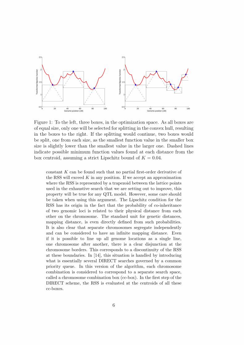
The original DIRECT algorithm initially creates a single searchbox covering the full search space, and the objective function, i.e.in our case the RSS, is evaluated in the center of this box. Thisbox is then split into three equally sized boxes along the majoringdimension. This trinary split results in the centroid of the originalbox coinciding with the centroid of one of the new boxes. Therefore,only two additional function evaluations are required for the threeresulting boxes. DIRECT then continues by iteratively splitting theboxes. At the end of each DIRECT iteration, the convex hull isdetermined among the remaining boxes, in a space of box radii vs.objective function values. This hull determines which boxes to splitin the following iteration. The selection is done based on the principleindicated above; if tracing along the box radii, the RSS value for thesequence of boxes is monotonously decreasing. Figure 1 illustrates afew iterations of DIRECT in a simple one-dimensional space. Thehull is “peeled off” when those boxes are split, making new boxesavailable in the next iteration. This process is repeated until a suitabletermination condition has been reached.

As has been remarked above, DIRECT implicitly assumes thatthe objective function is Lipschitz continuous. This means that a

5

0 20 40 60 80 1000.5

1

1.5

2

2.5

Genome position (cM)

Tra

nsfo

rmed

bje

ctiv

e fu

nctio

n

0 20 40 60 80 1000.5

1

1.5

2

2.5

Genome position (cM)

Tra

nsfo

rmed

bje

ctiv

e fu

nctio

n

Figure 1: To the left, three boxes, in the optimization space. As all boxes areof equal size, only one will be selected for splitting in the convex hull, resultingin the boxes to the right. If the splitting would continue, two boxes wouldbe split, one from each size, as the smallest function value in the smaller boxsize is slightly lower than the smallest value in the larger one. Dashed linesindicate possible minimum function values found at each distance from thebox centroid, assuming a strict Lipschitz bound of K = 0.04.

constant K can be found such that no partial first-order derivative ofthe RSS will exceed K in any position. If we accept an approximationwhere the RSS is represented by a trapezoid between the lattice pointsused in the exhaustive search that we are setting out to improve, thisproperty will be true for any QTL model. However, some care shouldbe taken when using this argument. The Lipschitz condition for theRSS has its origin in the fact that the probability of co-inheritanceof two genomic loci is related to their physical distance from eachother on the chromosome. The standard unit for genetic distances,mapping distance, is even directly defined from such probabilities.It is also clear that separate chromosomes segregate independentlyand can be considered to have an infinite mapping distance. Evenif it is possible to line up all genome locations as a single line,one chromosome after another, there is a clear disjunction at thechromosome borders. This corresponds to a discontinuity of the RSSat these boundaries. In [14], this situation is handled by introducingwhat is essentially several DIRECT searches governed by a commonpriority queue. In this version of the algorithm, each chromosomecombination is considered to correspond to a separate search space,called a chromosome combination box (cc-box). In the first step of theDIRECT scheme, the RSS is evaluated at the centroids of all thesecc-boxes.

6

If a bound on the Lipschitz constant K is known it is possible tocompute upper and lower bounds for the RSS within any box in thesearch space. However, when using the original DIRECT algorithm, Kis unknown. Note that it is still possible to impose a partial orderingof boxes; if a box A is both smaller and has a larger value of RSS thananother box B, then no value of K can result in a smaller minimumbound within A than within B.

DIRECT is part of the general family of Lipschitz optimizationschemes. Here, the more traditional schemes [19, 18, 8, 15] assumethat a bound of the Lipschitz constant is known. DIRECT deals withthe constant being unknown by always splitting the largest remainingbox, as a large enough value for K would allow the minimum pointto be located within the volume of that box. If a bound on K isknown when using DIRECT, known values of RSS in small boxes willalso enable exclusion of larger boxes, hereby introducing a pruning ofthe search tree. In contrast to the peeling effect of successive convexhulls in DIRECT, volumes excluded due to a Lipschitz criterion arepermanently irrelevant for further evaluation of the RSS.

The natural termination condition for such a modified DIRECTalgorithm is given by the finite resolution criterion corresponding tothe lattice in the underlying exhaustive search. This results in an errorbound of Kh on the value of the RSS, where h is the step length in thelattice. Thus, a bound on the Lipschitz constant K leads to improvedperformance (by more efficient exclusion), a well-defined error bound,and to a guarantee that the result is equivalent to the correspondingexhaustive search.

3 Linear Regression QTL Models

In this paper we consider QTL analysis for experimental populationswith known relations between individuals, and where the founderindividuals (the first generation in the pedigrees) have some origin-defining feature. This can be a matter of a known genetic relation (aset of common inbred or outbred lines) between the founders, or somefounders expressing a specific phenotype.

For ease of presentation, let us consider the typical case where wehave a F0 generation of individuals that can be considered to belongto either out of two lines, 0 and 1, so we consider each individual tocarry the genotype 00 or 11. If we make a cross of such individualsbetween the lines, we get a F1 generation. All those individuals willbe of 01 genotype (ordering aside), and so all variation between thoseindividuals would be environmental in nature.

From the F1 population, two other structures are commonly

7

considered. One is the backcross, where F1 individuals are crossedto F0 individuals from either line (say the 11s). This results in thatall individuals from that cross will be of 01/11 genotype, so thereare only two classes of individuals, allowing for considerable modelsimplicity. The other common structure results from crossing F1

individuals with each other, an intercross, yielding an F2 generationwith all genotypes 00/01/10/11 represented, in equal proportions (sohalf of all individuals will be of either heterozygote genotype).

If full genotype information is available the genotype informationat a specific locus can be expressed as an n×m indicator matrix Z, forn individuals and m possible genotypes. This mathematical formalismis consistent with the description in [1, 20]. The genetic effects arethen modeled as

G∗ = ZSE + ε. (1)

Here, the design matrix is the product of Z and S. The separationinto two matrices allows us to describe S independently of thespecific number of individuals in the population and their respectivegenotypes. The matrix S is ideally chosen to result in an orthogonalmodel, i.e. a model where independent estimates of variance can beassigned to the included effects (parameters), and where effects can beremoved from the model with no change to the estimated values andvariances for the remaining effects. To achieve this, the design matrixwill differ slightly between different loci, as the random sampling ofalleles in the analyzed population will not be perfectly uniform [16, 1].

The quality of a model can be determined by the portion of thetotal variance in the phenotype values that is explained by the model.A larger explained variance is equivalent to a smaller RSS for theregression, which is given by

∑ε2 in (1) above.

3.1 Explainable Variance as a Function of

Genetic Distance

We now consider several QTL search objective functions and examinetheir behavior at, and in the vicinity of, a QTL. The explainablegenetic variance is as such a natural objective function since theposition with minimum residual variance can be defined as thelocation of a putative QTL. The total phenotypic variance can thusbe decomposed as

Vtot = Vg + Vǫ. (2)

This definition assumes that all genetic variance is attributable

8

to the QTL. The residual variance, Vr, at the QTL position is thensimply Vr = Vǫ, or Vr = V − Vg. It is trivial to compute V , for anydata set, using only the phenotype observations. Hence, we can usethe function f(x) = V − Vr(x) as the objective function, just as wellas Vr(x) (which is proportional to the RSS) can be used directly. Theexpected value of Vr(x) can also be computed for any position x if weknow the recombination frequency p between the position denoted byx and the actual QTL, as well as the full variance Vg attributable tothe QTL.

Loci far apart on the same chromosome, or loci on differentchromosomes, will exhibit no linkage at all and any match will berandom. If, for simplicity, we assume a diallelic QTL in a backcrosspopulation with perfectly ideal allele frequencies, the probability p ofa second indicator matching an ideal indicator at the QTL will be 0.5.If the two indicators are identical (infinitely close), then p will be 1.0.All other situations are somewhere in between1.

If we now assume that the phenotype values for the two QTLgenotypes are 1 and 0, the variance with a null model (average only)will be 0.5(1−0.5)2+0.5(0−0.5)2 = 0.25. If we use an indicator of thereal genotype with accuracy p, we get two symmetrical classes, eachbeing a mixture of both actual genotypes. Below follows a derivationfor the residual variance of the “high” class (dominated by individualswith a 1 phenotype). Due to the symmetric structure, this is equal tothe total variance

Vr = p(1 − µ)2 + (1 − p)µ2 = p(1 − 2µ + µ2) + (1 − p)µ2, (3)

µ = 1.0(p) + 0.0(1 − p) = p,

Vr = p − p2.

Here, µ is the average value within the class as defined by theindicator. This is the “target” for the linear regression. As thevariance is 0.25 under the null hypothesis, the relative reduction invariance possible through the indicator is given by

V − Vr

V=

0.25 − Vr

0.25. (4)

In an actual genome with a known mapping distance x between theloci, p is equivalent to the complement to the recombination fraction.

1This assumes ignoring the possibility that some locus due to selection pressure actuallytends to show an inverted preferred heritage structure relative to the QTL. Furthermore,such a locus pair would not have a well-defined mapping distance, so this possibility isfrequently ignored at an earlier step in the experiment setup, i.e. the construction of themarker map.

9

If we assume no recombination interference, we can relate this tomapping distances through the Haldane mapping function[9], withx in cM (centimorgan)

p = 1 − 0.5(1 − e−2x100 ) = 0.5 + 0.5e−

2x100 . (5)

Inserting (5) for p in (3) and then inserting the result in (4), wearrive to a relative reduction in variance of

V − Vr(x)

V= e−

4x100 . (6)

The result will be similar if a different mapping function is used[13]. Thus, the variance at any point x, measured as the distance fromthe QTL defined in (2), is

Vr(x) = V − Vge− 4x

100 . (7)

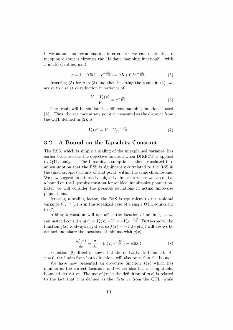
3.2 A Bound on the Lipschitz Constant

The RSS, which is simply a scaling of the unexplained variance, hasearlier been used as the objective function when DIRECT is appliedto QTL analysis. The Lipschitz assumption is then translated intoan assumption that the RSS is significantly correlated to the RSS inthe (macroscopic) vicinity of that point, within the same chromosome.We now suggest an alternative objective function where we can derivea bound on the Lipschitz constant for an ideal infinite-size population.Later we will consider the possible deviations in actual finite-sizepopulations.

Ignoring a scaling factor, the RSS is equivalent to the residualvariance Vr. Vr(x) is in this idealized case of a single QTL equivalentto (7).

Adding a constant will not affect the location of minima, so we

can instead consider g(x) = Vr(x)−V = −Vge−

|4x|100 . Furthermore, the

function g(x) is always negative, so f(x) = − ln(−g(x)) will always bedefined and share the locations of minima with g(x).

df(x)

dx=

d

dx− ln(Vge

−|4x|100 ) = ±0.04 (8)

Equation (8) directly shows that the derivative is bounded. Atx = 0, the limits from both directions will also be within the bound.

We have now presented an objective function f(x) which hasminima at the correct locations and which also has a computable,bounded derivative. The use of |x| in the definition of g(x) is relatedto the fact that x is defined as the distance from the QTL, while

10

a position in the chromosome can naturally be both upstream anddownstream from this position. It is possible to shift the functionby introducing the true QTL position y, resulting in f(x) = lnVg −0.04|x − y|.

We will now generalize the result above and demonstrate thatthe bound on K is maintained. First, we have assumed that allgenetic variance was attributable to a single locus (at y). We cannow assume a single-locus model for analysis, but that the trueQTL, with respective components of Vg are represented as a vectory = {y1, y2, ..., yn}, resulting in the following expression for theresidual variance (assuming all yi to be unlinked):

Vr(x) = V −

n∑

i=1

Vgie−

4|x−yi|

100 (9)

If all QTL are indeed unlinked, the positions yi relative to anyreference will be ±∞, except for at most one yj . Since linkage istransitive, the observation position x can at most be linked to a singleQTL. Thus, (9) reduces to

Vr(x) = V − Vgje

4|x−yj |

100 , (10)

and the derivative bound on (10) follows from the result in (8).The next extension is to make the search landscape itself multi-

dimensional, replacing the scalar x with a vector x = {x1, x2..., xm}.Assume that each xi is defined with a point of reference in linkage withthe corresponding QTL yi. Modeled locations not in linkage with anytrue QTL will result in no explainable variance, and therefore do notneed to be considered. As the numbering of both vectors is essentiallyarbitrary, all other cases are also symmetrical to this one. Using theearlier result, each xi will only have a term for the corresponding yi,as all other mapping distances |xi − yj | would be +∞. This results in

Vr(x) = V −n∑

i=1

Vgie−

4|xi−yi|

100 . (11)

We then have that

f(x) = − ln(−Vr(x) + V ), (12)

where the logarithm does not affect the location of minima.Equation (11) can be rewritten as

Vr(x) = V − Vgje−

4|xj−yj |

100 −n∑

i=1,i6=j

Vgie−

4|xi−yi|

100

︸ ︷︷ ︸

C

, (13)

11

for any arbitrary j ∈ N, j ≤ n. Based on (13), (12) becomes

f(x) = − ln(Vgje−

4|xj−yj |

100 + C). (14)

From basic calculus, we know that | ddx

ln(ekx + C)| = | kekx

ekx+C| ≤

ddx

ln(ekx) = kekxekx

= k for any C ∈ R, C ≥ 0. Hence, all partial

derivatives ∂f∂xj

are confined by the bound given for the single-

dimensional first derivative presented earlier. Thus, f(x) as definedabove will have a well-defined Lipschitz bound.

For a multi-locus case including interacting QTL (epistasis), theimportant observation to make is that the probability of a fully correctindication of the QTL genotype is pn (if assuming all xi approximatelyequal, or at least of the same order of magnitude), where p is again theprobability of a correct indication at a specific locus at a specific one-dimensional distance x. The logarithm is then approximately givenby

lnVG −4x1n

100. (15)

This results in a constant derivative of 0.04 for a single locus,0.08 for two interacting loci, 0.12 for three interacting loci, and soon. This is a very pessimistic approximation, basically assumingthere are no detectable main effects at all, all genetic variance beingattributable to the epistatic variance components when doing anorthogonal decomposition of variance [6].

For linked QTL, the picture is more complex. The effects fromdifferent QTL are, at least partially, confounded, as there is onlya single variable (the indicator position within the linkage group),relating back to both components. Among other things, this meansthat the total explainable variance can be 0 at some point in theregion between two linked QTL if the effects at the QTL have oppositesigns. However, outside of the interval between the linked QTL, thebehavior is completely identical to the presence of a single QTL atthe position of the closest QTL in the set, with an effect equivalent tothe combined average effect of all the linked QTL observed from thatposition. This can intuitively be understood from the memory-lessnature of the exponential function.

4 Using a practical bound

The bound derived does not apply directly to the derivative of theactual residual variance in the data, but to the expected value of

12

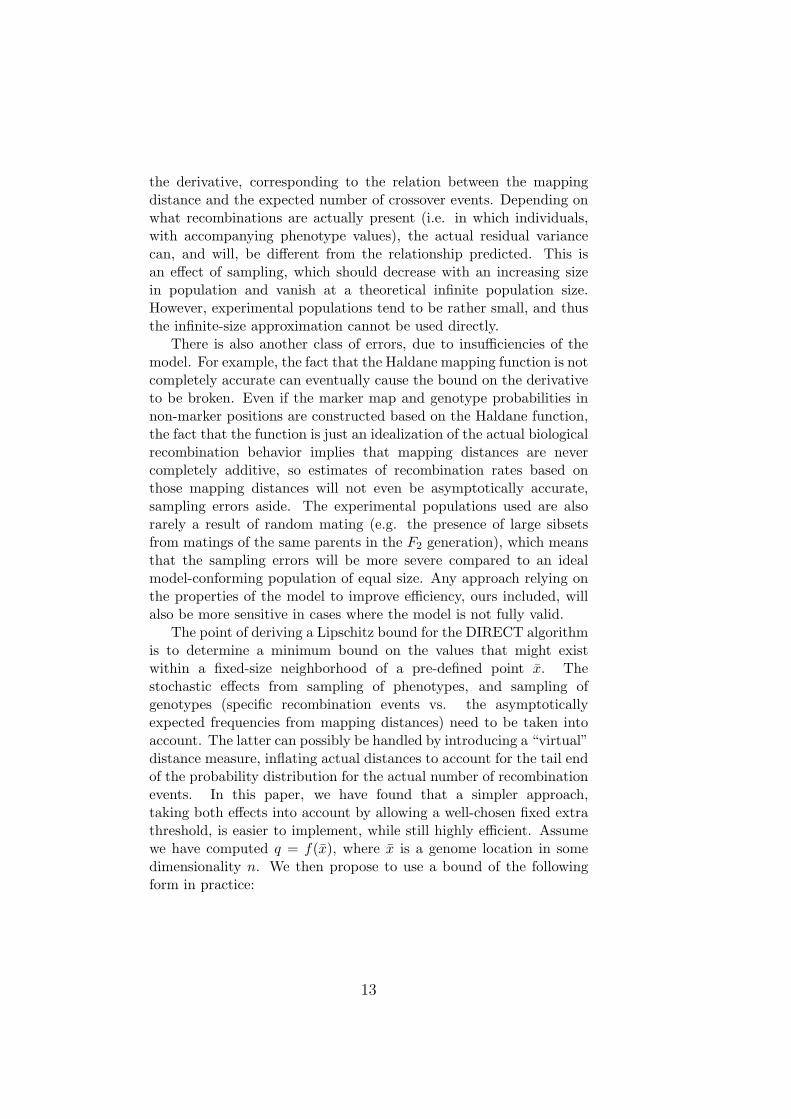
the derivative, corresponding to the relation between the mappingdistance and the expected number of crossover events. Depending onwhat recombinations are actually present (i.e. in which individuals,with accompanying phenotype values), the actual residual variancecan, and will, be different from the relationship predicted. This isan effect of sampling, which should decrease with an increasing sizein population and vanish at a theoretical infinite population size.However, experimental populations tend to be rather small, and thusthe infinite-size approximation cannot be used directly.

There is also another class of errors, due to insufficiencies of themodel. For example, the fact that the Haldane mapping function is notcompletely accurate can eventually cause the bound on the derivativeto be broken. Even if the marker map and genotype probabilities innon-marker positions are constructed based on the Haldane function,the fact that the function is just an idealization of the actual biologicalrecombination behavior implies that mapping distances are nevercompletely additive, so estimates of recombination rates based onthose mapping distances will not even be asymptotically accurate,sampling errors aside. The experimental populations used are alsorarely a result of random mating (e.g. the presence of large sibsetsfrom matings of the same parents in the F2 generation), which meansthat the sampling errors will be more severe compared to an idealmodel-conforming population of equal size. Any approach relying onthe properties of the model to improve efficiency, ours included, willalso be more sensitive in cases where the model is not fully valid.

The point of deriving a Lipschitz bound for the DIRECT algorithmis to determine a minimum bound on the values that might existwithin a fixed-size neighborhood of a pre-defined point x̄. Thestochastic effects from sampling of phenotypes, and sampling ofgenotypes (specific recombination events vs. the asymptoticallyexpected frequencies from mapping distances) need to be taken intoaccount. The latter can possibly be handled by introducing a “virtual”distance measure, inflating actual distances to account for the tail endof the probability distribution for the actual number of recombinationevents. In this paper, we have found that a simpler approach,taking both effects into account by allowing a well-chosen fixed extrathreshold, is easier to implement, while still highly efficient. Assumewe have computed q = f(x̄), where x̄ is a genome location in somedimensionality n. We then propose to use a bound of the followingform in practice:

13

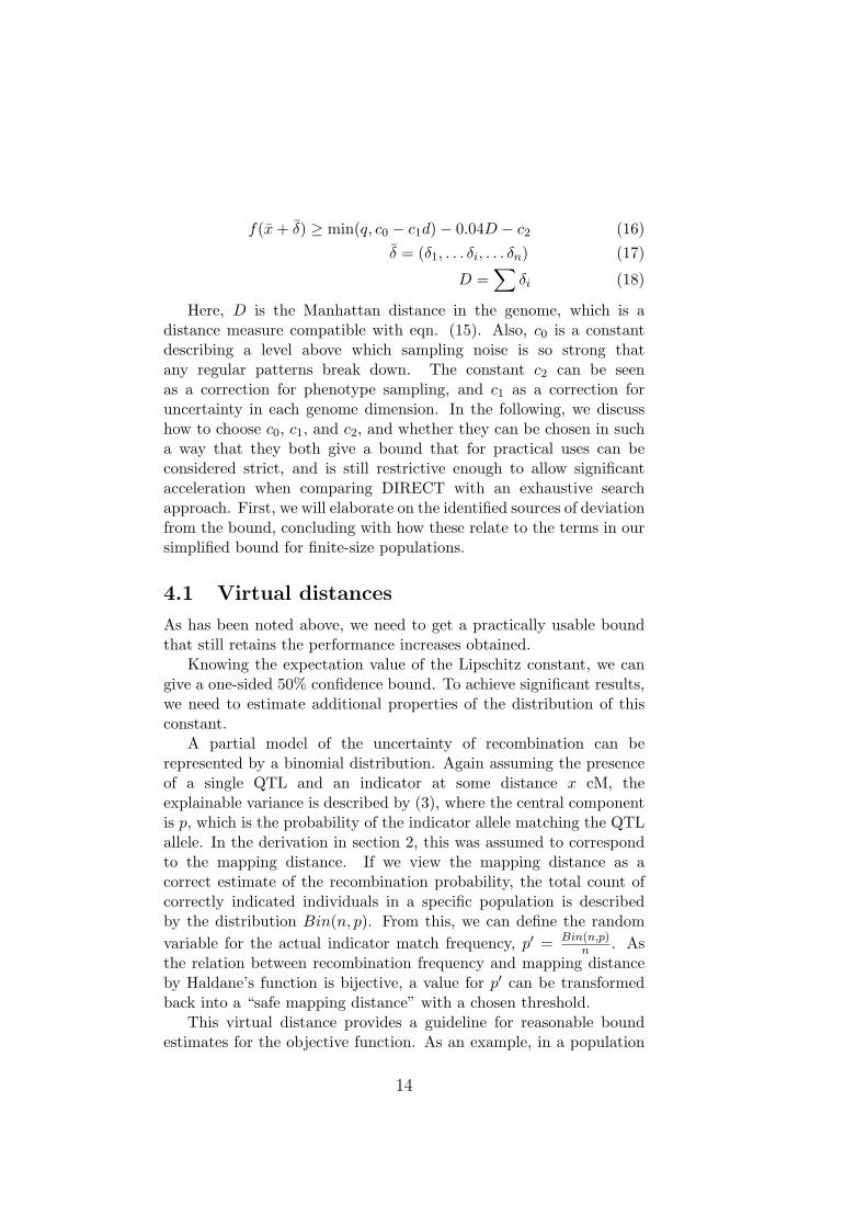
f(x̄ + δ̄) ≥ min(q, c0 − c1d) − 0.04D − c2 (16)

δ̄ = (δ1, . . . δi, . . . δn) (17)

D =∑

δi (18)

Here, D is the Manhattan distance in the genome, which is adistance measure compatible with eqn. (15). Also, c0 is a constantdescribing a level above which sampling noise is so strong thatany regular patterns break down. The constant c2 can be seenas a correction for phenotype sampling, and c1 as a correction foruncertainty in each genome dimension. In the following, we discusshow to choose c0, c1, and c2, and whether they can be chosen in sucha way that they both give a bound that for practical uses can beconsidered strict, and is still restrictive enough to allow significantacceleration when comparing DIRECT with an exhaustive searchapproach. First, we will elaborate on the identified sources of deviationfrom the bound, concluding with how these relate to the terms in oursimplified bound for finite-size populations.

4.1 Virtual distances

As has been noted above, we need to get a practically usable boundthat still retains the performance increases obtained.

Knowing the expectation value of the Lipschitz constant, we cangive a one-sided 50% confidence bound. To achieve significant results,we need to estimate additional properties of the distribution of thisconstant.

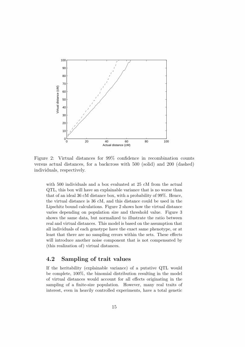
A partial model of the uncertainty of recombination can berepresented by a binomial distribution. Again assuming the presenceof a single QTL and an indicator at some distance x cM, theexplainable variance is described by (3), where the central componentis p, which is the probability of the indicator allele matching the QTLallele. In the derivation in section 2, this was assumed to correspondto the mapping distance. If we view the mapping distance as acorrect estimate of the recombination probability, the total count ofcorrectly indicated individuals in a specific population is describedby the distribution Bin(n, p). From this, we can define the random

variable for the actual indicator match frequency, p′ = Bin(n,p)n

. Asthe relation between recombination frequency and mapping distanceby Haldane’s function is bijective, a value for p′ can be transformedback into a “safe mapping distance” with a chosen threshold.

This virtual distance provides a guideline for reasonable boundestimates for the objective function. As an example, in a population

14

0 20 40 60 80 1000

10

20

30

40

50

60

70

80

90

100V

irtua

l dis

tanc

e (c

M)

Actual distance (cM)

Figure 2: Virtual distances for 99% confidence in recombination countsversus actual distances, for a backcross with 500 (solid) and 200 (dashed)individuals, respectively.

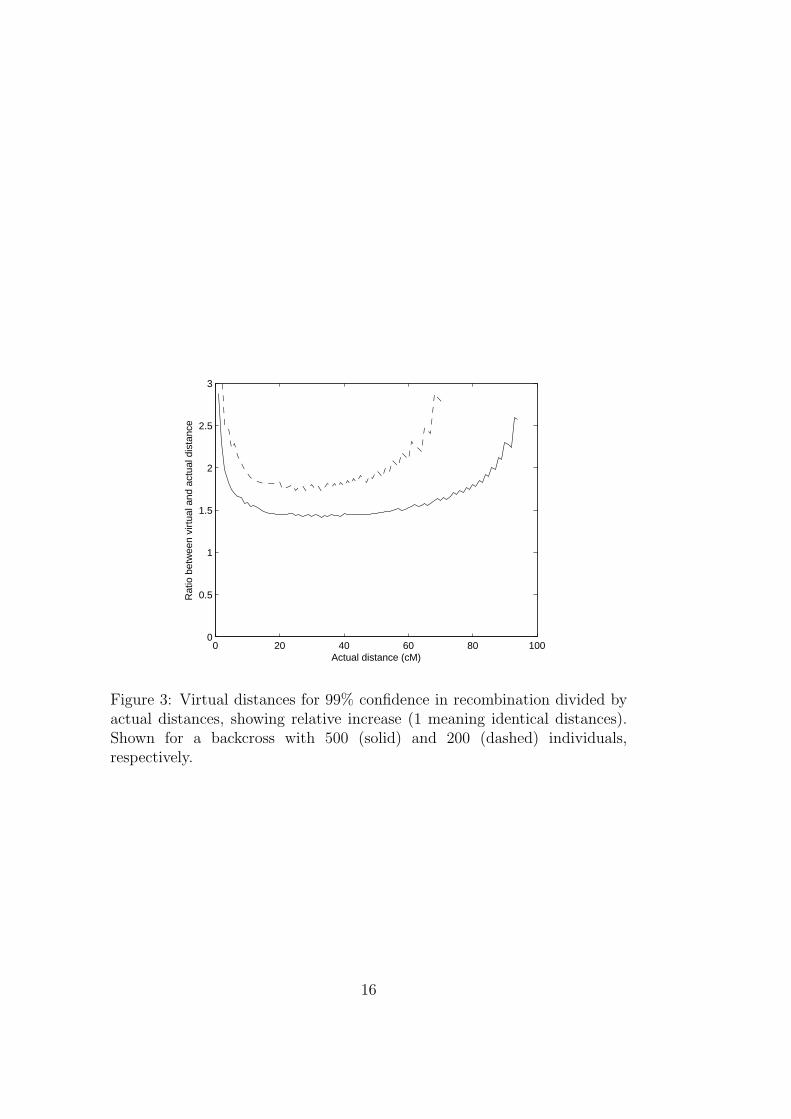
with 500 individuals and a box evaluated at 25 cM from the actualQTL, this box will have an explainable variance that is no worse thanthat of an ideal 36 cM distance box, with a probability of 99%. Hence,the virtual distance is 36 cM, and this distance could be used in theLipschitz bound calculations. Figure 2 shows how the virtual distancevaries depending on population size and threshold value. Figure 3shows the same data, but normalized to illustrate the ratio betweenreal and virtual distances. This model is based on the assumption thatall individuals of each genotype have the exact same phenotype, or atleast that there are no sampling errors within the sets. These effectswill introduce another noise component that is not compensated by(this realization of) virtual distances.

4.2 Sampling of trait values

If the heritability (explainable variance) of a putative QTL wouldbe complete, 100%, the binomial distribution resulting in the modelof virtual distances would account for all effects originating in thesampling of a finite-size population. However, many real traits ofinterest, even in heavily controlled experiments, have a total genetic

15

0 20 40 60 80 1000

0.5

1

1.5

2

2.5

3

Rat

io b

etw

een

virt

ual a

nd a

ctua

l dis

tanc

e

Actual distance (cM)

Figure 3: Virtual distances for 99% confidence in recombination divided byactual distances, showing relative increase (1 meaning identical distances).Shown for a backcross with 500 (solid) and 200 (dashed) individuals,respectively.

16

variance component of far less than 50%. Therefore, it is not enoughto consider what proportions of individuals correspond to the trueQTL genotype at a specific analyzed position. The recombinationprocess will introduce a shift in genotype in a random sample of theindividuals. The size of the sample is determined by the (virtual)recombination distance. However, the actual phenotype values of theindividuals shifted is also relevant. If the samples of individuals withinthe genotype groups (as defined by their true QTL genotype) havemeans that tend away from the other genotype, e.g. if the sampledindividuals are overrepresenting the tails of the total phenotypedistribution, the observed within-class means will get closer to eachother and thus the explainable variance will decrease further.

We can describe this by considering the set of all the populationto be P, of cardinality n. We once again consider the backcross, so wehave individuals in subsets P0,P1, reflecting their actual genotypeat some putative QTL. There is also observed genotype data atsome distance away, resulting in a division along another axis, in allresulting in subsets P00,P01,P10,P11. For each set Pi, there is acorresponding mean µi, cardinality ni and variance σ2

i . The geneticeffect is µ1−µ0 = a, and by translation we can assume µ0 = 0, µ1 = a.By scaling, we can assume the residual variance to be σ2

0 = σ21 = 1.

We can also assume the distribution at the locus itself to be ideal,n0 = n1 = n/2. The previously introduced recombination frequencyp can be used to determine the cardinality of the double-indexedsubsets, {n01, n10} = pn/2, {n00, n11} = (1 − p)n/2. In practice, thesymmetry in size n01 = n10 does not hold, due to the sampling effectsof recombination partially modeled through virtual distances.

The sampling of values will be directly manifested in the valuesof µ01 and µ10. In the expectation/median case, we will have simply{µ01, µ10} = {µ0, µ1}. According to the assumption that the residualvariance is normal, we want to know the distribution for the meanof a random sample of specific size n01 from a finite size normalpopulation of size n00. Thus, the normal distribution for the sample

mean is µ01 = N(

µ0,1

n01

n00

n0−1

)

, the second factor being the so-called

Finite Population Correction Factor. We can continue the assumptionn01 = n10 by assuming ∆µ = µ01 − µ0 = µ1 − µ10. The concept of anidentical ∆µ, and the value at all being a single constant, is naturallya simplification, but this theoretical modeling could be extended.The sampling effects for recombination frequency, and the samplingeffects due to varying phenotype means in the subsets of individualsactually showing recombinations over the distance considered, areclosely related. At this time we do not have a full analytical expressionfor these interactions.

17

4.3 Motivating our approximate bound

The critical observation to motivate the approximate bound 16 is thatthe sampling effects are expected to be strong for small sets, i.e. shortdistances. When few individuals are sampled, the freedom is muchgreater. For very short distances, this is true. The question can bewhether any recombination is occurring at all, and the change frome.g. 2 to 3 individual recombinations will affect the objective functionradically. The Lipschitz bound rather assumes recombinations to be acontinuous event, as would be the case in an infinite-size population.By including a constant threshold term in each dimension, we canaccount for both change in recombination counts, and an RSS-inflatingor RSS-deflating random sampling of the identity of the recombiningindividuals.

Furthermore, sampling effects are generally not expected to allgo in the same direction at the same time. The general safetythreshold applied at all points should not scale with the total numberof dimensions. This makes sense, since the real source of the trait valuesampling uncertainty is originating from the environmental variability,which is not specific to our model-dimension. A correction might beneeded for small population sizes, though.

Strong sampling effects due to small individual counts are notonly present in the case of short distances, but also very longdistances. The effects from a single individual recombining in thecorrect manner versus 50/50 proportions at unlinked positions can bedrastic. Therefore, we also include the upper bound q, which shouldbe chosen so that the explained variance found, compared to a modelwith no explainable variance (i.e. a +∞ objective function value), isexceeding a few individuals. The chance for such a division increaseswith a higher dimensionality, which is why the upper threshold shoulddecrease with the number of loci.

These three constants will need to be chosen based on populationsize, and population structure.

4.4 Application of the modified bound

With a higher genetic variance component, the global minimum willbe more extreme. This means that, once a minimum is found, there isa much greater opportunity of aggressive pruning in the search space,based on box sizes and the derivative bound. DIRECT will find thetrue global minimum, and fewer iterations will be needed for traitswith a higher heritability.

While attractive, this property also introduces a real problem,since the most frequent genome scan operation is often a run within a

18

random permutation test [5]. To get a significance threshold for 99%,it is prudent to do at least 2, 000 runs, compared to a single run forthe actual trait data. Since each permutation test run will include arandom permutation of the phenotype data, with unmodified genotypedata, the expected heritability in those runs is very close to 0. Indeed,the purpose of the test is to determine the expected “false” heritabilityin random data similar to that actually analyzed.

However, as the purpose of doing the random permutations is todetermine a significance threshold empirically, we will not need tolocate the exact QTL in the random data. Rather, it is enough toget one single boolean value out of each run: is it possible to finda QTL set in the permuted dataset with a residual variance belowthat of the actual trait set, or not? The process outlined belowcan also be adapted to handle the case of several candidate traitswith different variance levels. The distribution of outcomes is stillcompletely discrete: the random set may show a higher apparentheritability than all candidates, lie in the region between two of them,or be inferior to all of them (which is generally expected to be themost common result).

This results in one trivial termination condition, even without avalue of the Lipschitz constant K: if the residual variance detectedin a random set reaches a value below the known residual variancein the trait set, then immediate termination is possible, with a resultof true to the boolean test for that specific run. This scenario willbe relatively rare, however (5% of the tests if the trait might hit the95% threshold). Thanks to the value of K, we can also add the sameconstraint that was used in the search for the actual trait, i.e. boxeswhere the derivative bound precludes reaching a value below Vr (of theactual trait, not the random set) can be discarded. The only boxeswe need to explore are those that still might allow a lower residualvariance in the random data.

Thus, with the bound of K and the known Vr for the trait for whichwe are seeking significance, the same condition to discard boxes thatwere used in the end of the trait search can be applied from the start.This greatly accelerates the process, while simultaneously allowing ahigher number of iterations to be spent in those permuted sets thatactually might contain a random QTL above the intended threshold.This second observation is also important, since it might eliminate theproblem shown in some earlier studies regarding a bias for DIRECTin random permutation tests [14].

19

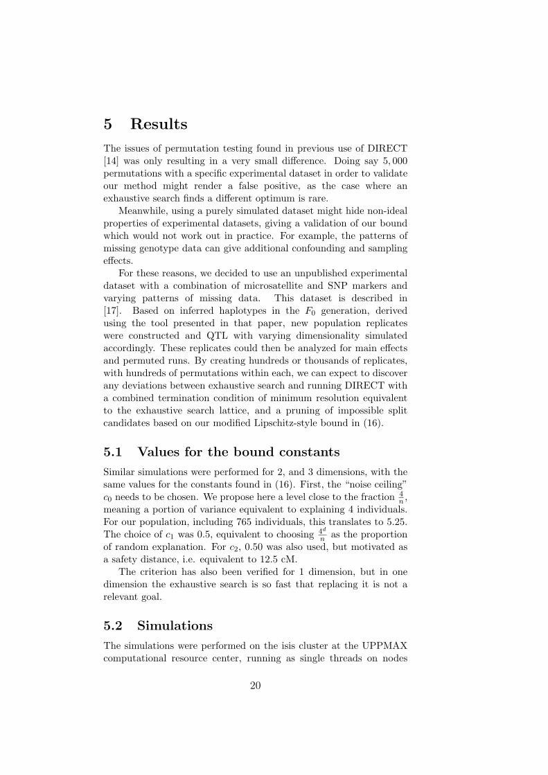
5 Results

The issues of permutation testing found in previous use of DIRECT[14] was only resulting in a very small difference. Doing say 5, 000permutations with a specific experimental dataset in order to validateour method might render a false positive, as the case where anexhaustive search finds a different optimum is rare.

Meanwhile, using a purely simulated dataset might hide non-idealproperties of experimental datasets, giving a validation of our boundwhich would not work out in practice. For example, the patterns ofmissing genotype data can give additional confounding and samplingeffects.

For these reasons, we decided to use an unpublished experimentaldataset with a combination of microsatellite and SNP markers andvarying patterns of missing data. This dataset is described in[17]. Based on inferred haplotypes in the F0 generation, derivedusing the tool presented in that paper, new population replicateswere constructed and QTL with varying dimensionality simulatedaccordingly. These replicates could then be analyzed for main effectsand permuted runs. By creating hundreds or thousands of replicates,with hundreds of permutations within each, we can expect to discoverany deviations between exhaustive search and running DIRECT witha combined termination condition of minimum resolution equivalentto the exhaustive search lattice, and a pruning of impossible splitcandidates based on our modified Lipschitz-style bound in (16).

5.1 Values for the bound constants

Similar simulations were performed for 2, and 3 dimensions, with thesame values for the constants found in (16). First, the “noise ceiling”c0 needs to be chosen. We propose here a level close to the fraction 4

n,

meaning a portion of variance equivalent to explaining 4 individuals.For our population, including 765 individuals, this translates to 5.25.The choice of c1 was 0.5, equivalent to choosing 4d

nas the proportion

of random explanation. For c2, 0.50 was also used, but motivated asa safety distance, i.e. equivalent to 12.5 cM.

The criterion has also been verified for 1 dimension, but in onedimension the exhaustive search is so fast that replacing it is not arelevant goal.

5.2 Simulations

The simulations were performed on the isis cluster at the UPPMAXcomputational resource center, running as single threads on nodes

20

Table 1: Size of validation tests for two and three dimensions. Time use for

validating exhaustive search runs limits the possible size for 3D. Permutations

were done per replicate.d Heritability (h2) Number of replicates Number of permutations2 0.09 500 10003 0.14 500 100

with AMD Optreon 2220 CPUs. The code is parallel, but since a veryhigh number of replicates were used, the serial version, with its highermemory locality and lack of synchronization overhead, was preferred.

For each run, first the non-permuted QTL model of specified sizewas fit, allowing all levels of interaction (each genotype-phenotypemean was a free parameter). Then, permutations were created. Forexhaustive search, all possible candidate loci sets were tried in a 1 cMlattice. For DIRECT, the minimum resolution was that same lattice,but in addition the bound was used to avoid splitting of some boxes,if it was definite that the values within that box could not improveon the minimum found in the original main run. The optimizationof terminating the full search when a minimum surpassing the onein the original was found, was not implemented. This occurrenceis supposed to be rare, but would reduce the maximum number offunction evaluations needed drastically. It would also be possible tostop after only a lower number of permutations, if it is already clearat that point that the original result will not be significant.

Table 1 presents the specific number of replicates, the simulatedbroad-sense heritability h2, and the number of permutations donefor each replicate. Table 2 presents average, minimum and mediannumber of function evaluations for complete sets of main run pluspermutations. Timings show that objective function evaluationsexceed 90% of the time used in the DIRECT version. For actualsignificance tests, a higher number of permutations would be prudent,but in order to properly validate the bound within reasonable time, ahigher number of replicates is supposed to contribute to a more variedtest set.

Out of our 500 simulations used in 2 dimensions, 34 were lessthan 99% significant. If these are removed from the computednumber of function evaluations, the average number of evaluationsdecreases to 7.78e5. Acceleration compared to exhaustive search isonly possible when the result from the main run rises above the noisefloor established by the constants in our bound.

21

Table 2: Number of function evaluations for two and three dimensions with

exhaustive search and DIRECT, respectively. Minimum, mean, median and

maximum number of function evaluations per full run of main QTL search

followed by the number of permutations given in Table 1 are reported. A very

low number of DIRECT runs resulted in full exhaustive searches. Note that

the 3-dimensional scan used a lower number of permutations.d Method Min Median Avg Maximum2

Exhaustive 7.88e6 7.88e6 7.88e6 7.88e6DIRECT 4.76e5 7.79e5 1.84e6 7.88e6

3Exhaustive 9.99e8 9.99e8 9.99e8 9.99e8DIRECT 2.81e5 1.21e6 2.76e6 3.98e7

6 Discussion

A hurdle against wide implementation of efficient global optimizationalgorithms for QTL searches have been the reluctance against methodswhich do not guarantee optimal results. The bound presented in thispaper, and the underlying theory, is a step towards providing suchguarantees.

Previous reported speedups for DIRECT in the QTL space havebeen several orders of magnitude. The work presented in this paperdoes not improve on those results. Instead, we provide an option forperforming the QTL scan where accuracy and guaranteed results areof higher importance. We do so by letting DIRECT continue executinguntil a full exhaustive search has in some sense been performed, butwith a pruning taking place removing boxes that are not possibleoptima. This allows DIRECT to be used not only for finding QTLcandidates, but also to be reliably used in permutation testing tofind the extreme end of the null hypothesis distribution. Thesecomputations can be used to compute significance thresholds as well asassessing the extreme value distribution, something which could forma basis for comparisons between models with different dimensionalityand parametrization.

We finally propose to use a derivative bound which is of ad-hocform, but this is based on a thorough analysis and reformulation of theobjective function. This reformulation accelerates the performance ofDIRECT, even when the pruning step is not added. The performanceimprovement is easily understood, as DIRECT will perform best ifthe function is linear (finding the top of a single triangle in only a few

22

iterations), and the transformation used will in general transform theobjective function to be almost piecewise linear. This understandingof the expected local form of the objective function, when full genotypeinformation is available, could also be used to better assess probableQTL locations in cases of partial and incomplete genetic information.We can also note that our empirically determined thresholds for c0, c1

correspond quite well to a correction for the number of degrees offreedom in the model. If this can be verified and mathematicallyproven, the general validity of the bound would be further ensured.The choice of c2 will still be complicated, as it is used to correct forthe non-ideal distribution of recombination events.

It should be noted that the performance for our version of DIRECTis dependent on the heritability. For a trait with no heritability atall, finding the true optimum can in principle only be done by anexhaustive search, as very limited correlations are expected in theobjective function between loci. Previous incarnations of DIRECTwould have failed in those cases, while our modified implementationis adaptive and will perform more function evaluations. If one knowsbeforehand that QTL with a heritability below some limit h2

min arenot relevant, then such information can be added to our pruning andgive better performance even in those cases.

If the goal is to establish the significance of a QTL with very highsignificance, then our approach will excel. If most null hypothesispermutations for a dataset have a minimum that is inferior to thatdetermined for the main model, the permuted DIRECT runs canexit after only a hundred or so function evaluations, even in multipledimensions. This allows doing runs equivalent to 100, 000 or morepermutations for loci where significance levels above 99.9% would berelevant.

References

[1] J. M. Alvarez-Castro and O. Carlborg. A Unified Modelfor Functional and Statistical Epistasis and Its Application inQuantitative Trait Loci Analysis. Genetics, 176(2):1151–1167,2007.

[2] M. Bogdan, J. K. Ghosh, and R. W. Doerge. Modifyingthe Schwarz Bayesian Information Criterion to Locate MultipleInteracting Quantitative Trait Loci. Genetics, 167(2):989–999,2004.

[3] E. A. Carbonell, T. M. Gerig, E. Balansard, and M. J. Asins.

23

Interval mapping in the analysis of nonadditive quantitative traitloci. Biometrics, 48(1):305–315, 1992.

[4] O. Carlborg, L. Andersson, and B. Kinghorn. The use of a ge-netic algorithm for simultaneous mapping of multiple interactingquantitative trait loci. Genetics, 155:2003–2010, 2000.

[5] G. Churchill and R. Doerge. Empirical threshold values forquantitative trait mapping. Genetics, 138:963–971, 1994.

[6] C. C. Cockerham. An extension of the concept of partitioninghereditary variance for analysis of covariances among relativeswhen epistasis is present. Genetics, 39(6):859–882, 1954.

[7] R. Doerge. Mapping and analysis of quantitative trait lociin experimental populations. Nature reviews-Genetics, 3:43–52,2002.

[8] E. Galerpin. The cubic algorithm. J of Mathematical Analysis

and Applications, pages 635–640, 1985.

[9] J. B. S. Haldane. The combination of linkage values, and thecalculation of distance between the loci of linked factors. J Genet,8:299–309, 1919.

[10] C. S. Haley and S. A. Knott. A simple regression method formapping quantitative trait loci in line crosses using flankingmarkers. Heredity, 69(4):315–24, 1992.

[11] R. C. Jansen. Interval Mapping of Multiple Quantitative TraitLoci. Genetics, 135(1):205–211, 1993.

[12] D. Jones, C. Perttunen, and B. Stuckman. Lipschitzian optimiza-tion without the lipschitz constant. J. Optimization Theory App,79:157–181, 1993.

[13] E. S. Lander and D. Botstein. Mapping Mendelian FactorsUnderlying Quantitative Traits Using RFLP Linkage Maps.Genetics, 121(1):185–199, 1989.

[14] K. Ljungberg, S. Holmgren, and O. Carlborg. Simultaneoussearch for multiple QTL using the global optimization algorithmDIRECT. Bioinformatics, 20(12):1887–1895, 2004.

[15] R. Mladineo. An algorithm for finding the global maximum of amultimodal, multivariate function. Mathematical Programming,pages 253–271, 1987.

24

[16] C. Nettelblad, O. Carlborg, and J. M. Alvarez-Castro. Efficientalgorithms for multi-dimensional global optimization in geneticmapping of complex traits. Technical report 2010-005, Divisionof Scientific Computing,Dept of IT, Uppsala University, 2010.

[17] C. Nettelblad, S. Holmgren, L. Crooks, and O. Carlborg. cnf2freq:Efficient determination of genotype and haplotype probabilitiesin outbred populations using markov models. In S. Rajasekaran,editor, BICoB 2008, volume 5462 of Lecture Notes in Computer

Science, pages 307–319. Springer, 2009.

[18] J. Pinter. Globally convergent methods for n-dimensional multi-extremal optimization. Optimization, 17:187–202, 1986.

[19] B. Shubert. A sequential method seeking the global maximumof a function. SIAM J. on Numerical Analysis, pages 379–388,1972.

[20] Z.-B. Zeng, T. Wang, and W. Zou. Modeling Quantitative TraitLoci and Interpretation of Models. Genetics, 169(3):1711–1725,2005.

25