stock annex: sardine (sardina pilchardus) in divisions 8.a ... reports/stock...

ICES Stock Annex | 1

Stock Annex: Sardine (Sardina pilchardus) in divisions 8.a–b and 8.d and in Subarea 7 (Bay of Biscay, southern Celtic Seas, and the English Channel)

Stock specific documentation of standard assessment procedures used by ICES.

Stock: Sardine

Working Group: Working Group on Anchovy and Sardine and Southern Horse Mackerel (WGHANSA)

Created:

Authors:

Last updated: 4-8 February 2013 (WKPELA)

Last updated by: E. Duhamel, L. Ibaibarriaga, J. Massé, L. Pawlowski, M. Santos and A. Uriarte

A. General

A.1. Stock definition

European sardine (Sardine pilchardus Walbaum, 1792) has a wide distribution extend-ing in the Northeast Atlantic from the Celtic Sea and North Sea in the north to Mauri-tania in the south. Populations of Madeira, the Azores and the Canary Islands are at the western limit of the distribution (Parrish et al., 1989). Sardine is also found in the Mediterranean and the Black Seas. Changing environmental conditions affect sardine distribution, with fish having been found as far south as Senegal during episodes of low water temperature (Corten and van Kamp, 1996; Binet et al., 1998).

Sardine in Celtic Seas (7.a,b,c,f,g,j,k), English Channel (7.d, 7.e, 7.h) and in Bay of Biscay (8.a,b,d) are considered to belong to the same stock from a genetic point of view. There-fore, the sardine stock in 8.a,b,d and 7. can be considered as a single stock unit but it is important to note that there should be some distinction within the stock structure to take account of some regional differences between fisheries as there are some locally important fisheries operating in some area.

The availability of data strongly differs between the northern (Celtic Seas, English Channel) and the southern component (Bay of Biscay). Additionally, each area presents different historical exploitation patterns. Therefore analysis and management advice between the areas may differ, even if the advice covers the whole stock.

A.2. Fishery

There are currently no management measures implemented for this stock. The fisheries appear to be regulated by market price. Some fisheries (e.g. French fleets in the Bay of Biscay) have set their own local management in order to sustain correct market prices which imply targeting fish of certain sizes and limit to the total amount of catch. The absence of TAC is currently not seen as a problem for the management of those fisher-ies as the demand of sardine is considered to be low.

| 2 ICES Stock Annex

Divisions 8.a,b,d (Bay of Biscay)

An update of the French and Spanish catch dataseries in Divisions 8.a and 8.b (from 1983 and 1996 for France and Spain, respectively) including 2011 catches was presented to this benchmark. Spanish catches are taken by purse seines from the Basque Country operating only in Division 8.b. Spanish landings peaked in 1998 and 1999 with almost 8 thousand tonnes but have decreased until 2010 to below 1 thousand tonnes. The Spanish fishery takes place mainly during March and April and in the fourth quarter of the year.

French catches have increased along the series, with values ranging from 4400 tonnes in 1983 to 23 000 tonnes in 2011 (Figure A.2.1). A total of 90% of the catches are taken by purse seiners while the remaining 10% is reported by pelagic trawlers (mainly pair trawlers). A substantial part of the French catches originates in Divisions 7.h and 7.e, but these catches have been assigned to Division 8.a due to their very concentrated location at the boundary between 8.a, 7.h and 7.e.

Spanish catches were unusually high prior 1989 where a strong drop occurs. The rea-son of this drop is unknown and likely to be related to some data aggregation issues which make any uses of landings prior this year uncertain.

Both purse seiners and pelagic trawlers target sardine in French waters. Average vessel length is about 18 m. Purse seiners operate mainly in coastal areas (<10 nautical miles) while trawlers are allowed to fish within 3 nautical miles from the coast. Both pair trawlers and purse seiners operate close to their base harbour when targeting sardine. The highest catches are taken in the summer months. Almost all the catches are taken in southwest Brittany.

While French catches in Divisions 8.a and 8.b are constituted by fish of a wide range of sizes with a peak at 20 cm length, sardine taken by Spanish vessels show a narrower range of sizes but with a peak at similar length size.

The Bay of Biscay sardine fisheries overlaps with 7.e and 7.h (statistical rectangle 25E4, 25E5). Catches in those rectangles are assumed to be of sardine from Bay of Biscay. Therefore landings in Bay of Biscay and English Channel are corrected to take account of this phenomenon by adding the catches in those rectangles to the Bay of Biscay land-ings time-series.


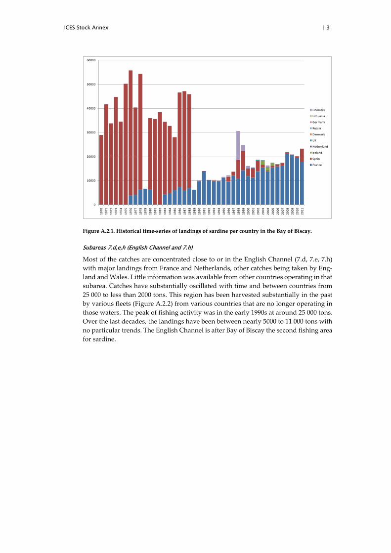
Figure A.2.1. Historical time-series of landings of sardine per country in the Bay of Biscay.

Subareas 7.d,e,h (English Channel and 7.h)

Most of the catches are concentrated close to or in the English Channel (7.d, 7.e, 7.h) with major landings from France and Netherlands, other catches being taken by Eng-land and Wales. Little information was available from other countries operating in that subarea. Catches have substantially oscillated with time and between countries from 25 000 to less than 2000 tons. This region has been harvested substantially in the past by various fleets (Figure A.2.2) from various countries that are no longer operating in those waters. The peak of fishing activity was in the early 1990s at around 25 000 tons. Over the last decades, the landings have been between nearly 5000 to 11 000 tons with no particular trends. The English Channel is after Bay of Biscay the second fishing area for sardine.

0

10000

20000

30000

40000

50000

60000

1970

1971

1972

1973

1974

1975

1976

1977

1978

1979

1980

1981

1982

1983

1984

1985

1986

1987

1988

1989

1990

1991

1992

1993

1994

1995

1996

1997

1998

1999

2000

2001

2002

2003

2004

2005

2006

2007

2008

2009

2010

2011

Denmark

Lithuania

Germany

Russia

Denmark

UK

Netherland

Ireland

Spain

France


Figure A.2.2. Historical time-series of landings of sardine per country in the English Channel and 7.h.

As mentioned for the Bay of Biscay, catches in rectangles 25E4, 25E5 are removed from the official landings and added to the catches in the Bay of Biscay to take account of the mixing at the borders of Division 8.a and 7.h and 7.e.

Subareas 7.a,b,c,f,g,j,k (Celtic Seas)

Catches in this area are very low.

A.3. Ecosystem aspects

Sardine is prey of a range of fish and marine mammal species which take advantage of its schooling behaviour and availability. Sardine has been found to be important in the diet of common dolphins (Delphinus delphis) in Galicia (NW Spain) (Santos et al., 2004), Portugal (Silva, 2003) and the Atlantic French coast (Meynier, 2004). Recent studies of consumption of common dolphins in Galician (Santos et al., 2011) waters give figures ranging from almost 6000 tons to more than 9000 tons of sardine, which represents a rather small proportion of the combined Spanish and Portuguese annual landings of sardine from ICES Areas 8.c and 9.a (6–7%).There are also other species feeding on sardine, although to a lesser extent, such as: harbour porpoise (Phocoena phocoena), bot-tlenose dolphin (Tursiops truncatus), striped dolphin (Stenella coeruleoalba), and white-sided dolphin (Lagenorhynchus acutus) (e.g. Santos et al., 2007).

B. Data

B.1. Commercial catches

Landings data have been available for since 1950 on various aggregation levels. Data are considered to be accurate for all countries starting 1989 within the whole area. Dis-cards were measured only in 2012 and were low based on the French Observers at sea program in the Bay of Biscay and hence not included in the assessment. In the past (late eighties and early nineties for the French Pelagic trawlers and sixties and seventies for

0

5000

10000

15000

20000

25000

30000

1970

1971

1972

1973

1974

1975

1976

1977

1978

1979

1980

1981

1982

1983

1984

1985

1986

1987

1988

1989

1990

1991

1992

1993

1994

1995

1996

1997

1998

1999

2000

2001

2002

2003

2004

2005

2006

2007

2008

2009

2010

2011

Denmark

Germany

Russia

Lithuania

Ireland

UK

Netherland

France


the Spanish Purse seine fleet) they seemed to be more relevant (according to disputes among fishermen), but were never quantified. Length distribution of discards are also available from Netherlands in the English Channel for 2011.

B.2. Biological

• Catches-at-length and catches-at-age are known since 1984 for Spain and since 2002 for France in the Bay of Biscay. Because of the availability of the datasets only the period starting in 2000 is used. They are obtained by ap-plying to the monthly Length distributions half year or quarterly ALKs. Bi-ological sampling of the catches has been generally sufficient, and useful to have a better knowledge of the age structure of the catches during the sec-ond semester in the North of the Bay of Biscay. Complete age composition and mean weight-at-age on half year basis, were each year reported in ICES (WGHANSA report, ICES 2012).

• Age reading is considered accurate. The most recent cross reading ex-changes and workshop between Spain and France (but other countries, too) took place in 2011 (WKARAS report, ICES 2011). The overall level of agree-ment and precision in sardine of the Bay of Biscay age reading determina-tions seems to be satisfactory: Most of the sardine otoliths were well classified by most of the readers during the 2011 workshop (with an average agreement 75% and a CV of 14%).

• Sardines are mature in their 1st year of life.

• Growth in weight and length are routinely obtained from surveys and from the monitoring of the fishery.

• Natural mortality is fixed at 0.33 based on the assessment for sardine in 8.c and 9.a. This parameter is considered to vary between years and ages, but it is assumed to be constant for the assessment of the stock.

B.3. Surveys

Relevant surveys are available for the Bay of Biscay only. Some sardines are caught during the various demersal surveys (e.g FR-IBTS) occuring each year in the Celtic Seas, Bay of Biscay and English Channel but those catches are not substantial enough to be considered as indicators of the stock status.

Some abundance indices are available every year for the Bay of Biscay through two spring surveys based on acoustic surveys (PELGAS) and DEPM (Daily egg production method - BIOMAN).

The population present in the Bay of Biscay is monitored by the two annual surveys carried out in spring on the spawning stock, namely, the Daily Egg Production Method and the Acoustics surveys (regularly since 1989, although surveys were also conducted in 1983, 1984 and some in the seventies) (Massé, 1988; 1994; 1996). Both surveys provide spawning biomass and population-at-age estimates.

This survey based monitoring system provides population estimates by the middle of the year, when a small part of the annual catches have been already taken.

B.3.1. Sardine acoustic indices (PELGAS survey)

Acoustic surveys are carried out every year in the Bay of Biscay in springon board the French research vessel Thalassa since 1997. The objective of PELGAS surveys is to study the abundance and distribution of pelagic fish in the Bay of Biscay.


These surveys are connected with Ifremer programmes on data collection for monitor-ing and management of fisheries and ecosystemic approach for fisheries. This task is formally included in the first priorities defined by the Commission regulation EU N° 199/2008 of 06 November 2008 establishing the minimum and extended Community programmes for the collection of data in the fisheries sector and laying down detailed rules for the application of Council Regulation (EC) No 1543/2000. These surveys must be considered in the frame of the Ifremer fisheries ecology action "resources variability" which is the French contribution to the international Globec programme. It is planned with Spain and Portugal in order to have most of the potential area to be covered from Gibraltar to Brest with the same protocol for sampling strategy. Data are available for the ICES working groups WGHANSA, WGWIDE and WGACEGG.

In 2003, survey data are considered less reliable because of unusual environmental con-ditions linked to the heat wave over Europe. Results this year were considered not representative of the true status of the stock.

B.3.1.1. PELGAS Method and sampling strategy

In the frame of an ecosystemic approach, the pelagic ecosystem is characterised at each trophic level. In this objective, to assess an optimum horizontal and vertical description of the area, two types of actions are combined:

• Continuous acquisition by storing acoustic data from five different frequen-cies and pumping seawater under the surface in order to evaluate the num-ber of fish eggs using a CUFES system (Continuous Under-water Fish Eggs Sampler); and

• Discrete sampling at stations (by trawls, plankton nets, CTD). Satellite im-agery (temperature and sea colour) and modelisation will be also used be-fore and during the cruise to recognise the main physical and biological structures and to improve the sampling strategy. Concurrently, a visual counting and identification of cetaceans and birds (from board) is carried out in order to characterise the higher level predators of the pelagic ecosys-tem.

Satellite imagery (temperature and sea colour) and modelisation are also used before and during the cruise to recognise the main physical and biological structures and to improve the sampling strategy.

The strategy of the survey is the same for the whole series (since 2000).

• Acoustic data were collected along systematic parallel transects perpendic-ular to the French coast (Figure B.3.1.1). The length of the ESDU (Elementary Sampling Distance Unit) was 1 mile and the transects were uniformly spaced by 12 nautical miles covering the continental shelf from 20 m depth to the shelf break.

• Acoustic data were collected only during the day because of pelagic fish be-haviour in this area. These species are usually dispersed very close to the surface during the night and so "disappear" in the blind layer for the echo sounder between the surface and 8 m depth.

Two echo-sounders are usually used during surveys (SIMRAD EK60 for vertical echo-sounding and MARPORT on the pelagic trawl). Since 2009 the SIMRAD ME70 is used for multibeam visualisation. Energies and samples provided by split beam transducers (six frequencies EK60, 18, 38, 70, 120, 200 and 333 kHz), simple beam (MARPORT) and


multibeam echosounder were simultaneously visualised, stored using the MOVIES+ software and at the same standard HAC format.

The calibration method is the same that the one described for the previous years (see W.D. 2001) with a tungsten sphere hanged up 20 m below the transducer and is gener-ally performed at anchorage in front of Machichaco Cap or in the Douarnenez Bay, on the west side of Brittany, in optimal meteorological conditions.

Acoustic data are collected by Thalassa along the totality of the daylight route from which about 2000 nautical miles on one way transect are usable for assessment. Fish are measured on board (for all species) and otoliths (for anchovy and sardine) are col-lected for age determinations.

Figure B.3.1.1. The acoustic transects network of the PELGAS survey.

B.3.1.2. Echoes scrutinizing

Most of the acoustic data along the transects are processed and scrutinised during the survey and are generally available one week after the end of the survey. Acoustic en-ergies (Sa) are cleaned by sorting only fish energies (excluding bottom echoes, para-sites, plankton, etc.) and classified into several categories of echotraces according to the year fish (species) structures.

D1 – energies attributed to mackerel, horse mackerel, blue whiting, various demersal fish, corresponding to cloudy schools or layers (sometimes small dis-persed points) close to the bottom or of small drops in a 10 m height layer close to the bottom.

D2 – energies attributed to anchovy, sprat, sardine and herring corresponding to the usual echo-traces observed in this area since more than 15 years, consti-tuted by schools well defined, mainly situated between the bottom and 50 me-ters above. These echoes are typical of clupeids in coastal areas and sometimes more offshore.


D3 – energies attributed to blue whiting, myctophids and boarfish offshore, just closed to the shelf-break and on the platform in the north.

D4 – energies attributed to sardine, mackerel and anchovy corresponding to small and dense echoes, very close to the surface.

D8 – energies attributed exclusively to sardine (big and very dense schools).

B.3.1.3. Data processing

The global area is split into several strata where coherent communities are observed (species associations) in order to minimise the variability due to the variable mixing of species. For each stratum, a mean energy is calculated for each type of echoes and the area measured. A mean haul for the strata is calculated to get the proportion of species into the strata. This is obtained by estimating the average of species proportions weighted by the energy surrounding haul positions. Energies are therefore converted into biomass by applying catch ratio, length distributions and TS relationships. The calculation procedure for biomass estimate and variance is described in Petitgas et al.,2003.

The TS relationships used since 2000 are still the same and as following:

Sardine, anchovy & sprat: TS = 20 Log L – 71.2

Horse mackerel: TS = 20 Log L – 68.7

Blue whiting: TS = 20 Log L – 67.0

Mackerel: TS = 20 Log L – 86.0

The mean abundance per species in a stratum (tons m.n.-2) is calculated as:

),(),()( kDXkDskM eD

Ae ∑=

and total biomass (tons) by: )()( kMekABk

e ∑=

where,

k : strata index

D : echo type

e : species

SA: Average SA (NASC) in the strata (m2/n.mi.2)

Xe : species proportion coefficient (weighted by energy around each haul) (tons m-2)

A : area of the strata (m.n.2)

Then variance estimate is:

),(.)],(var[)(.)],([),()(. 22 kDesunkDsXkchankDXVarkDskMVar AeeD

Ae +=∑

)(.)(. 2 kMeVarkABVark

e ∑=

BeBeVarcv .=

At the end, density in numbers and biomass by length and age are calculated for each species in each ESDU according to the nearest haul length composition. These numbers


and biomass are weighted by the biomass in each stratum and data are used for spatial distributions by length and age.

The detailed protocol for these surveys (strategy and processing) is described in Annex 6 of WGACEGG report (ICES 2009).

B.3.2. Anchovy Daily Egg Production Method (BIOMAN Survey)

B.3.2.1. The DEPM model

The sardine spawning–stock biomass estimates is derived according to Parker (1980) and Stauffer and Picquelle (1980) from the ratio between daily production of eggs in the sea and the daily specific fecundity of the adult population:

Equation 1 WSFRkAP

DFPSSB tot

⋅⋅⋅+⋅

== 0

Where,

SSB = Spawning–stock biomass in metric tons

Ptot= Total daily egg production in the sampled area

P0= daily egg production per surface unit in the sampled area

A+ = Spawning area, in sampling units

DF = Daily specific fecundity. W

SFRkDF ⋅⋅⋅=

W = Average weight of mature females in grams,

R = Sex ratio, fraction of population that are mature females, by weight.

F= Batch fecundity, numbers of eggs spawned per mature females per batch

S= Fraction of mature females spawning per day

k = Conversion factor from gram to metric tons (106)

An estimate of an approximate variance and bias for the biomass estimator derived using the delta method (Seber, 1982, in Stauffer and Picquelle, op. cit.) was also devel-oped by the latter authors.

Population estimates of numbers-at-age are derived as follows:

Equation 2 a

taa E

WSSBENN ⋅=⋅=

Where,

Na = Population estimate of numbers-at-age a.

N = Total spawning–stock estimate in numbers. tW

SSBN =

SSB = spawning–stock biomass estimate.

Wt= average weight of anchovies in the population.


Ea = Relative frequency (in numbers) of age a in the population.

Variance estimate of the sardine stock in numbers-at-age and total is derived applying the delta method.

B.3.2.2. Collection of plankton samples

Every year the area covered to collect the plankton samples is the southeast of the Bay of Biscay taking in advance the anchovy survey in the Bay of Biscay.

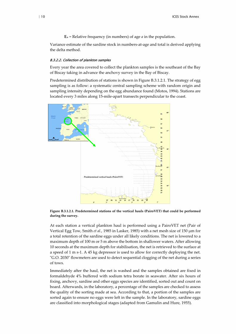
Predetermined distribution of stations is shown in Figure B.3.1.2.1. The strategy of egg sampling is as follow: a systematic central sampling scheme with random origin and sampling intensity depending on the egg abundance found (Motos, 1994). Stations are located every 3 miles along 15-mile-apart transects perpendicular to the coast.

Figure B.3.1.2.1. Predetermined stations of the vertical hauls (PairoVET) that could be performed during the survey.

At each station a vertical plankton haul is performed using a PairoVET net (Pair of Vertical Egg Tow, Smith et al., 1985 in Lasker, 1985) with a net mesh size of 150 µm for a total retention of the sardine eggs under all likely conditions. The net is lowered to a maximum depth of 100 m or 5 m above the bottom in shallower waters. After allowing 10 seconds at the maximum depth for stabilisation, the net is retrieved to the surface at a speed of 1 m s-1. A 45 kg depressor is used to allow for correctly deploying the net. "G.O. 2030" flowmeters are used to detect sequential clogging of the net during a series of tows.

Immediately after the haul, the net is washed and the samples obtained are fixed in formaldehyde 4% buffered with sodium tetra borate in seawater. After six hours of fixing, anchovy, sardine and other eggs species are identified, sorted out and count on board. Afterwards, in the laboratory, a percentage of the samples are checked to assess the quality of the sorting made at sea. According to that, a portion of the samples are sorted again to ensure no eggs were left in the sample. In the laboratory, sardine eggs are classified into morphological stages (adapted from Gamulin and Hure, 1955).

282930

27

3132333435

37

39

41424344454647

49

51

53

2523211917151311Bi

Bordeaux

SS

Arcachon

Santander

Nantes

47°

46°

45°

44°

6° 5° 4° 3° 2° 1°

48°

La Rochelle

0907

55

57

59

61

Predetermined vertical hauls (PairoVET)


The Continuous Underway Fish Egg Sampler (CUFES, Checkley et al., 1997) is used to record the eggs found at 3 m depth with a net mesh size of 350 µm. The CUFES system has a CTD to record simultaneously temperature and salinity at 3 m depth, a flowmeter to measure the volume of the filtered water, a fluorimeter and a GPS (Geographical Position System) to provide sampling position and time. All these data are registered at real time using the integrated EDAS (Environmental Data Acquisition System) with custom software.

During the survey, the anchovy, sardine and other eggs are recorded per PairoVET station and the area where sardine eggs occurred is quantified. Following the system-atic central sampling scheme (Cochran, 1977) each station is located in the centre of a rectangle. Egg Abundance found at a particular station is assumed to represent the abundance in the whole rectangle. The area represented by each station is measured. A standard station has a surface of 45 squared nautical miles (154 km2) = 3 (distance between two consecutive stations) x 15 (distance between two consecutive transects) nautical miles. Since sampling is adaptive, station area changed according to sampling intensity and the cut of the coast.

Sample depth, temperature, salinity and fluorescence profiles are obtained in every station using a CTD RBR-XR420 coupled to the PairoVET. In addition, surface temper-ature and salinity is recorded in each station with a manual termosalinometer WTW LF197.Moreover current data are obtained all along the survey with an ADCP (Acous-tic Doppler Current Profiles). In some point determinate previously to the survey, wa-ter is filtered from the surface to obtain chlorophyll samples to calibrate the chlorophyll data.

B.3.2.3. Collection of adult samples

Since 2008 each three years adults are being obtained from a research vessel with pe-lagic trawl taking in advance the anchovy survey.

The research vessel pelagic trawler covers the same area as the plankton vessel. When the plankton vessel encountered areas with sardine eggs, the pelagic trawler is directed to those areas to fish. In each haul 100 individuals of each species are measure. Imme-diately after fishing, sardine is sorted from the bulk of the catch and a sample is selected at random. A minimum of 60 anchovies are weighted, measured and sexed and from the mature females the gonads of 25 non-hydrated females (NHF) are preserved. If the target of 25 NHF is not completed 10 more anchovies are taken at random and process in the same manner. Sampling is stopped when 120 anchovies have to be sexed to achieve the target of 25 NHF. Otoliths are extracted on board and read in the laboratory to obtain the age composition per sample.

B.3.2.4. Total daily egg production estimates

Since 1999 the sardine eggs were counted but only were staged in years 1999, 2002, 2008 and 2011.

In years without egg stages it was considered the total abundances of eggs defined as the sum along all the stations of the sardine eggs in each station multiplied by the area each station represents.

In years when sardine eggs are sorted and staged (1999, 2002, 2008 and 2011), it is pos-sible to estimate total daily egg production (Ptot). This is calculated as the product be-tween the daily egg production (P0) and the spawning area (SA).

SAPPtot 0=


A standard sampling station represents a surface of 45 nm2 (i.e. 154 km2). Since the sampling was adaptive, area per station changes according to the sampling intensity and the cut of the coast. The total area is calculated as the sum of the area represented by each station. The spawning area (SA) is delimited with the outer zero sardine egg stations but it can contain some inner zero stations embedded. The spawning area is computed as the sum of the area represented by the stations within the spawning area.

The daily egg production per area unit (P0) was estimated together with the daily mor-tality rate (Z) from a general exponential decay mortality model of the form:

(2) ( )jiji aZPP ,0, exp −=

,

where Pi,j and ai,j denote respectively the number of eggs per unit area in cohort j in station i and their corresponding mean age. Let the density of eggs in cohort j in station i, Pi,j, be the ratio between the number of eggs Ni,j and the effective sea area sampled Ri (i.e. P i,j = N i,j / Ri). The model was written as a generalised linear model (GLM, McCullagh and Nelder, 1989; ICES, 2004) with logarithmic link function:

(3) ( ) ( ) jiiji aZPRNE ,0, log)log(][log −+=

,

where the number of eggs of daily cohort j in station i (Nij) was assumed to follow a negative binomial distribution. The logarithm of the effective sea surface area sampled (log(Ri)) was an offset accounting for differences in the sea surface area sampled and the logarithm of the daily egg production log(P0) and the daily mortality Z rates were the parameters to be estimated.

The eggs collected at sea and sorted into morphological stages had to be transformed into daily cohort frequencies and their mean age calculated in order to fit the above model. For that purpose the Bayesian ageing method described in ICES (2004), Stratou-dakis et al., (2006) and Bernal et al., (2011) was used. This ageing method is based on the probability density function (pdf) of the age of an egg f(age | stage, temp), which is constructed as:

(4) )(),|(),|( ageftempagestageftempstageagef ∝ .

The first term f(stage | age, temp) is the pdf of stages given age and temperature. It represents the temperature dependent egg development, which is obtained by fitting a multinomial model like extended continuation ratio models (Agresti, 1990) to data from temperature dependent incubation experiments (Ibaibarriaga et al., 2007, Bernal et al., 2008). The second term is the prior distribution of age. A priori the probability of an egg that was sampled at time τ of having an age is the product of the probability of an egg being spawned at time τ - age and the probability of that egg surviving since then (exp( -Z age)):

(5) ) exp( )()( ageZagespawnfagef −−=∝ τ .

The pdf of spawning time f(spawn=τ - age) allows refining the ageing process for spe-cies with spawning synchronicity that spawn at approximately certain times of the day (Lo, 1985a; Bernal et al., 2001). Sardine spawning time was assumed to be normally distributed with mean at 21:00h GMT and standard deviation of 3 (ICES, 2004). The peak of the spawning time was also used to define the age limits for each daily cohort (spawning time peak plus and minus 15 hours). Details on how the number of eggs in each cohort and the corresponding mean age are computed from the pdf of age are


given in Bernal et al. (2011). The incubation temperature considered was the one ob-tained from the CTD at 10 m in the way up.

Given that this ageing process depends on the daily mortality rate which is unknown, an iterative algorithm in which the ageing and the model fitting are repeated until con-vergence of the Z estimates was used (Bernal et al., 2001; ICES, 2004; Stratoudakis et al., 2006). The procedure is as follows:

Step 1. Assume an initial mortality rate value;

Step 2. Using the current estimates of mortality calculate the daily cohort fre-quencies and their mean age;

Step 3. Fit the GLM and estimate the daily egg production and mortality rates. Update the mortality rate estimate;

Step 4. Repeat steps (1)–(3) until the estimate of mortality converged (i.e. the difference between the old and updated mortality estimates was smaller than 0.0001).

Incomplete cohorts, either because the bulk of spawning for the day was not over at the time of sampling, or because the cohort was so old that its constituent eggs had started to hatch in substantial numbers, were removed in order to avoid any possible bias. At each station, younger cohorts were dropped if they were sampled before twice the spawning peak width after the spawning peak and older cohorts were dropped if their mean age plus twice the spawning peak width was over the critical age at which less than 99% eggs were expected to be still unhatched. Once the final model estimates were obtained the coefficient of variation of P0 was given by the standard error of the model intercept (log(P0)) (Seber, 1982) and the coefficient of variation of Z was ob-tained directly from the model estimates.

The analysis was conducted in R (www.r-project.org). The ”MASS” library was used for fitting the GLM with negative binomial distribution and the ”egg” library (http://sourceforge.net/projects/ichthyoanalysis/) for the ageing and the iterative algo-rithm.

B.3.2.5. Adult parameters, daily fecundity and SSB estimates

In 2008 and 2011 adult samples were collected within the same day as the egg sam-pling. These samples are used to obtain adult parameters to estimate the daily fecun-dity, i.e. batch fecundity, spawning fraction, average female weight and sex ratio.

These adult parameters are estimates as follows:

Sex Ratio (R): It is calculate as the average sample ratio between the average female weight and the sum of the average female and male weights of the anchovies in each of the samples.

Total weight of hydrated females is corrected for the increase of weight due to hydra-tion. Data on gonad-free-weight (Wgf) and correspondent total weight (W) of nonhy-drated females is fitted by a linear regression model. Gonad-free-weight of hydrated anchovies is then transformed to total weight by applying the following equation:

gfWbaW ∗+−=

For the Batch fecundity (F) estimates i.e. number of eggs laid per batch and female, the hydrated egg method was followed (Hunter et al, 1985). The number of hydrated oo-cytes in gonads of a set of hydrated females is counted. This number is deduced from

http://www.r-project.org/

http://sourceforge.net/projects/ichthyoanalysis/


a sub-sampling of the hydrated ovary: Three pieces of approximately 50 mg are re-moved from different parts of each ovary, weighted with precision of 0.1 mg and the number of hydrated oocytes counted. Sanz and Uriarte (1989) showed that three tissue samples per ovary are adequate to get good precision in the final batch fecundity esti-mate and the location of sub-samples within the ovary do not affect it. Finally the number of hydrated oocytes in the subsample is raised to the total gonad of the female according to the ratio between the weights of the gonad and the weight sub-sampled.

A linear regression between female weight and batch fecundity is established for the subset of hydrated females and used to calculate the batch fecundity of all mature fe-males. The average of the batch fecundity estimates for the females of each sample as derived from the gonad free weight–eggs per batch relationship is then used as the sample estimate of batch fecundity.

Moreover, an analysis is conducted to verify if there are differences in the batch fecun-dity if strata are defined to estimate SSB.

To estimate Spawning Frequency (S), i.e. the proportion of females spawning per day, was estimated from the incidence of postovulatory follicles 1 and 2 day old in the gon-ads of mature females (Hunter and Macewicz, 1985) (the number of females with Day-0 POF was corrected by the average number of females with Day-1 or Day-2 POF).

Mean and variance of the adult parameters are estimated following equations for clus-ter sampling (as suggested by Picquelle and Stauffer, 1985):

Equation 3

M

y M = Y

i

n

1=i

ii

n

1=i

∑

∑

Equation 4 1) - (n n M

Y) - y( M = Var(Y) 2

i2

i2

n

1=i∑

Where,

Yi is an estimate of whatever adult parameter from sample i and Mi is the size of the cluster corresponding to sample i. occasionally a station produced a very small catch, resulting in a small sub-sample size. To reflect the actual size of the station and its lower reliability, small samples were given less weight in the estimate. For the estima-tion of W, F and S, a weighting factor was used, which equalled to 1 when the number of mature females in station i (Mi) was 20 or greater and it equalled to Mi/20 otherwise. In the case of R when the total weight of the sample was less than 800 g then the weighting factor was equal to total weight of the sample divided by 800 g, otherwise it was set equal to 1. In summary for the estimation of the parameters of the Daily Fecun-dity we are using a threshold-weighting factor (TWF) under the assumption of homo-geneous fecundity parameters within each stratum.

The Spawning–Stock Biomass is estimates as the ratio between the total egg production (Ptot) and Daily Fecundity (DF).


B.3.2.6. Egg abundance estimates 1999–2012

Table B3.2.6.1. Sardine egg abundances in the Bay of Biscay from 1999 to 2012.

Ab.tot.Sp is the sum along all the stations of the sardine eggs in each station multiplied by the area each station represents. Pos.area is the positive area for sardine; tot area is the total area surveyed; %pos area is the percentage the positive area represents in relation to the total area and Ptot is the total egg production.

Figure B3.2.6.1. Total sardine egg abundance estimates from 1999 to 2012 in the Bay of Biscay.

Ab.tot_Sp pos area tot area % pos area Ab.tot/pos.area Ptot(egg/day) 1.3E+12 26,679 59,193 45 5.0E+07 7.8E+11 5.0E+12 40,139 52,212 77 1.2E+08 9.2E+11 14,547 51,629 28 6.3E+07 8.3E+12 39,112 50,951 77 2.1E+08 4.4.E+12 2.8E+12 22,878 47,927 48 1.2E+08 9.2E+12 37,289 49,446 75 2.5E+08 1.1E+13 38,979 50,202 78 2.8E+08 3.8E+12 23,376 45,413 51 1.6E+08 2.3E+12 16,710 45,499 37 1.4E+08 9.4E+12 20,235 46,501 44 4.6E+08 6.0.E+12 7.53E+12 34,746 60,733 57 2.2E+08 1.06.E+13 36,361 61,940 59 2.9E+08 4.50.E+12 22,851 98,405 23 2.0E+08 available 5.68E+12 20,054 80,381 25 2.8E+08

0.0E+001.0E+122.0E+123.0E+124.0E+125.0E+126.0E+127.0E+128.0E+129.0E+121.0E+131.1E+131.2E+13

1999 2000 2001 2002 2003 2004 2005 2006 2007 2008 2009 2010 2011 2012


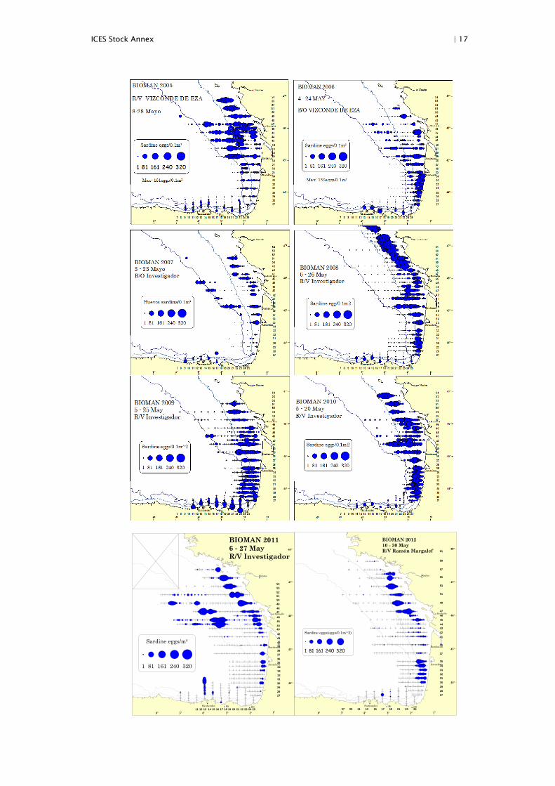
B.3.2.7 Historical series DEPM and acoustic surveys


282930

27

31323334353637383940414243444546

4748495051525354

252423222120191817161514131211Bi SS

Bordeaux

Arcachon

Santander

Nantes

47°

46°

45°

44°

6° 5° 4° 3° 2° 1°

48°

La Rochelle

BIOMAN 20116 - 27 MayR/V Investigador

Sardine eggs/m²

1 81 161 240 320

282930

27

3132333435

37

39

41424344454647

49

51

53

2523211917151311Bi

Bordeaux

SS

Arcachon

Santander

Nantes

47°

46°

45°

44°

6° 5° 4° 3° 2° 1°

48°

La Rochelle

0907

55

57

59

61

BIOMAN 201210 - 30 MayR/V Ramón Margalef

Sardine eggs(eggs/0.1m^2)

1 81 161 240 320


B.3.3. Sardine Daily Egg Production Method (SAREVA Survey) in the inner of the Bay of Biscay

B.3.3.1. Introduction

The Daily Egg Production Method (DEPM) is a well-established methodology to assess the spawning biomass (SSB) of fish species with indeterminate fecundity. The Sardine DEPM is based on the equation (Picquelle and Stauffer, 1985; Lasker, 1985):

RSFWPAreaSSB

***0*+

=

Where

P0: Daily egg production (eggs/m2/day)

Area +: Spawning area

W: Average weight of mature females in grams

F: Batch fecundity, number of eggs spawned per mature female per batch

S: Spawning fraction, fraction of mature females spawning per day

R: Sex Ratio is the fraction of the mature population that are females by weight.

The Daily Egg Production Method (DEPM) for sardine has been applied by Instituto Español de Oceanografía (IEO) to estimate the spawning–stock biomass of the North Atlanto-Iberian sardine stock since 1988 (García et al., 1992) and then repeated in 1990, 1997, 1999, 2002, 2005, 2008 and 2011. From 2000 onwards the surveys have been planned and conducted within the framework of ICES, on a triennial basis. Spring surveys for the application of the DEPM, consisting of ichthyoplankton, adults and hydrographic sampling, and since 1997 the sampling area was extended in order to reach the 45 degrees latitude North, covering the region from the northwestern (border Minho River), north Iberian Peninsula (north Spanish Atlantic and Cantabrian waters, ICES Division 9.a North and 8.c) and the inner part of the Bay of Biscay (from 42 ºN to 45°N, ICES Division 8.b).

This section provides a description of the sampling, laboratory analysis and estimation procedures used to obtain the sardine spawning–stock biomass estimate for the appli-cation of DEPM conducted by IEO from 1997 to present in the inner of the Bay of Biscay (ICES Division 8.b). Since 2002 extra effort was put in place in order to standardize methodologies for surveying, laboratorial and data analyses. These objectives were possible due to methodological developments and effective coordination undertaken first by the SGSBSA (ICES 2002–2004) and later by the WGACEGG (Stratoudakis et al., 2004; Stratoudakis et al., 2006; ICES, 2009; ICES, 2010; ICES, 2011).

Estimations for area delimitation (surveyed & spawning), egg ageing, mortality and model fitting for egg production (P0) are presented. Results from adults fishing sam-pling are showed and parameters from the mature fraction of the population (mean females weight, sex ratio, batch fecundity and spawning fraction) are calculated. Esti-mates were based on procedures and software adapted and developed during the WKRESTIM 2009 and modifications carried out subsequently for the revision of the sardine DEPM historical series (1988–2011) in Divisions 9.a and 8.c.

Sardine DEPM estimates in the inner of the Bay of Biscay (the inner part of Divisions 8.b until 45˚N) from 1997 until 2011, were presented in ICES Working Group on Acous-tic and Egg Surveys for Sardine and Anchovy in ICES Areas 8. and 9. (WGACEGG)


last November of 2012, in order to be considered as a contribution for the ICES WKPELA 2013 meeting for sardine in Subarea 7. and Divisions 8.a, b, d.

B.3.3.2. Methodology

B.3.3.2.1. Surveying

From 1997, six DEPM surveys were carried out by IEO (1997, 1999, 2002, 2005, 2008 and 2011). The Spanish surveys were undertaken using two vessels, RV Cornide de Saa-vedra for plankton sampling mainly and RV Thalassa to carry out the fishing hauls (in 2008 and 2011 some fishing hauls were carried out on RV Cornide de Saavedra). The surveys were designed to obtain an adequate spatial and temporal coverage during the spawning peak of sardine in the area. Due to the bad weather, in 2005 was not possible to complete the plankton sampling coverage, so no data for this year is presented in this work.

Plankton sampling

The main egg sampler for the DEPM is the PairoVET net that collects eggs through the water column at point stations. The PairoVET sampler (=double CalVET) includes two nets (Ø 25cm) with 150 µm mesh size; sampling covered the water column from bot-tom, or 100 m (beyond the 100 isobath) depth, to the surface. Vertical plankton hauls were carried out following a pre-defined grid (Figure 3.3.2.1.1) of sampling stations along transects perpendicular to the coast and spaced 8 miles from 2005 onwards. The inshore limit of the transects is determined by bottom depth (as close to shore as pos-sible) while the offshore extension was decided adaptively, based on the presence of eggs and covering the extension of the platform to the 200 m isobath.

From 2002, the Continuous Underway Fish Egg Sampler (CUFES) was used as an aux-iliary egg sampler, helping in defining the offshore extension of the transects and to modify adaptively the intensity of CalVET sampling. The outer limit of a transect was reached when two consecutive CUFES samples were negative beyond the 200 m depth.

From 1997 to 2005, a CTD (Sea Bird-25) profile (Temperature and Salinity) was carried out in each CalVET station. From 2008 to 2011 the Sea Bird-25 was used in each transect head and in alternate stations along the transects, meanwhile a CTD (Sea Bird-37) was coupled to the CalVET sampler. General Oceanics Flowmeters were used to record the towing length and estimate the sampled water volume (assuming a filtration efficiency of 100%).

After hauling, nets are washed from the outside with seawater under pressure and plankton samples from the two nets are preserved in formalin at 4% in distilled water and the two samples from each net stored in separate containers. Samples for one net are then sorted, and sardine, anchovy and other eggs are identified and counted. The total numbers of eggs from both plankton samplers, CalVET and CUFES, were counted onboard in order to obtain a preliminary data of sardine egg abundance and distribu-tion.


Figure 3.3.2.1.1. Sardine DEPM IEO surveys in the inner of the Bay of Biscay. Sardine egg distribu-tion (eggs/m2 from PairoVET sampler) and SST (ºC) by year.

Adult fish surveying

Fishing hauls were conducted by pelagic trawling following sardine schools detection by the echosounder (for RV Thalassa). The number of samples and its spatial distribu-tion was organized to ensure good and homogeneous coverage of the survey area (Fig-ure 3.3.2.1.2) in order to obtain a representation of the sardine population.

Onboard the RV, and for each haul, a minimum of 60 sardines were randomly selected and biologically sampled. These could also be complemented by additional fish in or-der to achieve a minimum of 30 females per haul for histology, and/or to obtain extra hydrated females for the fecundity estimations. The biological sampling was always carried out in fresh material, and ovaries were immediately collected and preserved in a formaldehyde buffered solution (4% diluted in distilled water) for posterior histolog-ical processing and analysis at the laboratory. Moreover, otoliths were extracted on board to obtain the age composition per sample in the laboratory.


Figure 3.3.2.1.2. Sardine DEPM IEO surveys in the inner of the Bay of Biscay. Spatial distribution of the positive fishing hauls by year.

B.3.3.2.2. Laboratorial analysis

Plankton samples

In the laboratory, all sardine eggs were sorted from PairoVET samples. The eggs from the vertical hauls (one net) were all counted and staged according to the eleven stages of development classification (adapted from Gamulin and Hure, 1955). Samples for the second net are used for plankton biomass quantification.

Adult fish samples

The preserved ovaries were weighted in laboratory and the obtained weights corrected by a conversion factor (between fresh and formaldehyde fixed material) established previously. These ovaries were processed for histology, first, they were embedded in resin (paraffin before 2005), the histological sections were stained with haematoxylin and eosin, and then the slides examined and scored for their maturity state, POF pres-ence and age assignment (Hunter and Macewicz, 1985; Pérez et al., 1992a; Ganias et al., 2007). Prior to fecundity estimation, hydrated ovaries were also processed histologi-cally in order to check for POF presence and thus avoid underestimating fecundity (Pérez et al., 1992b). The individual batch fecundity was then measured, by means of the gravimetric method applied to the hydrated oocytes, on 1–3 whole mount subsam-ples per ovary, weighting on average 50–150 mg (Hunter et al., 1985).

B.3.3.2.3. Data analysis

Databases with date, time, position, bottom depth and other variables registered dur-ing the sampling on board and in the laboratory, were merged in a common standard-ised dataset (eggs and adults data separately) and include all surveys undertaken in the period from 1997 to 2011. The dataset for eggs and adults include minor corrections (e.g. wrong geographical coordinates, duplicated points, ovary and total weights data,

-4º -3º -2º -1º

43º

44º

45º

19971999200220082011

Fishing hauls


etc.), that were observed as mistakes in a first exploration data. All estimations and statistical analysis were performed using the R software (www.r-projet.org).

Egg data

Calculations for area delimitation, egg ageing and model fitting for egg production (P0) estimation were carried out using the R packages (geofun, eggsplore and shachar) availa-ble within the open source project ichthyoanalysis (http://sourceforge.net/projects/ich-thyoanalysis). Some routines of the R packages used were updated since the 2008 versions.

The coastline and depth contour were imported from the GEBCO coastline, trans-formed into spatial objects to be used with the statistical software R. The limits of the survey area (sampled) and positive area (area with eggs), both offshore and coastal, were estimated using the library geofun, which mainly use the spatial analysis func-tionality provided by spatstat. To define the precision of the poligons to be selected, a 600x600 resolution was used in the spatstat function (spatstat.op-tions(npixel=c(600,600)).

To find the geographical limits of sampled and positive areas the findlimits.fun func-tion was used. The procedure includes an automated routine using neighbourhood distance, in km, between stations (minimum distance in ratio represented by each sta-tion). The routine thus generates circles around each sampling point and uses the in-tercepts between circles to define the sampling area. To estimate the limits of the sampled area, the argument dist was set to 15 km (findlimits.fun (data, dist = 15, plot = “limits”)) and all the sampled stations were used in the analysis.

The limits of the spawning area (positive area) were obtained using only those stations with eggs, the diameter of the circles was the same referred above (15 km) allowing embedment of negative stations fully surrounded by positive stations. After this initial delimitation of positive area, the function erode.owin (with diameter = 10 km) was used to reduce the external limits of the positive area, in order to limit the amount of negative (offshore) stations included in the positive area. With this trimming only the negative stations on the borders are excluded from the positive areas. The stations within that domain are flagged as positive and thereafter used in the analyses. Both the survey and total areas were afterwards corrected to avoid extrapolation to the coast, by computing the intercept between the areas estimated as above and the area delim-ited by the coastline.

To avoid high and low extremes values detected in the area represented by each sam-pled station, the parameter “area.range” was forced to the minimum and maximum values of 25 and 175 respectively (the extreme values usually occur on the borders of the survey area and therefore do not affect the estimation of the positive area). The area.range parameter was included in the estimate.sea.area function during the present analyses to avoid over estimation of the areas on the borders of the survey limits. The range 25–175 was selected to be a mean interval suitable for all the surveys, according to the distance between transect and stations (that varied in the initial years; from 2002 onwards it was fixed to be 8 nm between transects and 3 or 6 nm between stations, along transects).

The area represented by each station within the survey limits is estimated by a dirichlet tessellation of the survey stations, using the survey limits as estimated above. The pos-itive area is the sum of the areas of the individual stations included in the positive area (including also the negative stations embed in the positive area).

http://sourceforge.net/projects/ichthyoanalysis

http://sourceforge.net/projects/ichthyoanalysis


The model of egg development with temperature was derived from the incubationex-periment data available within the sardata R library. Egg ageing was achieved by amultinomial Bayesian approach described by Bernal et al. (2008) and using in situ SST.

depm.control function from egg package, controls some constants for DEPM as the as-sumption of spawning peak, the proportion of eggs that must still be unhatched (i.e. not transformed to larvae) at “2*sig” past the last cohort mean age (how.complete) and the distribution of the daily spawning cycle. For the present analyses the distribution of the daily spawning cycle was assumed as a normal (Gaussian) distribution, with a peak at 21:00 h GMT and a standard deviation of 3 h. (spawning period from 21-6 h to 21+6 hours). It is assumed that 0 time is at midnight and days are 24 hours long.

The upper age cutting limit was determined using a maximum age for the entire area considered and it is not dependent on the individual stations (upper.age=F). Older co-horts are dropped if their mean age plus 2* st-dev hours is over the critical age at which less than 5% of the eggs are expected to be still unhatched (how.complete=95%). The lower age cutting excluded the first cohort of stations in which the sampling time is included within the daily spawning period (lower.age=T).

The exponential model: E [P] = P0 e -Z age was fitted as a Generalized LinearModel (GLM) with negative binomial distribution and log link. For 1999 survey a model with-out mortality was applied since an estimate for mortality led to non-coherent mortality. Weights proportional to the relative area represented by each station (estimated using the dirichlet tessellation and divided by the mean area represented by a station) were used to account for increased sampling in areas of expected high egg densities.

Finally, the total egg production is calculated multiplying the daily egg production ratio (eggs per m2 and day) by the positive area (in m2).

Ptot =P0 *A+

Fish data

The adult parameters estimated for each fishing haul considered only the mature frac-tion of the population (determined by the fish macroscopic maturity data) and was based on the biological data collected from surveys. For the present estimations, a minimum sample criterion (n = 30) was introduced: a few hauls containing less than 30 fish sampled were excluded from the mean and variance calculations.

Before the estimation of the mean female weight per haul (W), the individual total weight (Wt) of the hydrated females was corrected by a linear regression between the total weight of non-hydrated females and their corresponding gonad-free weight (Wnov). The sex ratio (R) in weight per haul was obtained as the quotient between the total weight of females on the total weight of males and females.

The fraction of females spawning per day (S) was determined, for each haul, as the average number of females with Day-1 or Day-2 POF, divided by the total number of mature females (the number of females with Day-0 POF was corrected by the average number of females with Day-1 or Day-2 POF, and the hydrated females were not in-cluded).

In 1999 no histology samples were available to estimate spawning fraction (S) and a non-parametric bootstrap approach was performed using mean spawning fraction by each haul obtained along the all series and considering a single haul as the basic sam-pling unit. Hauls were resampling with replacement from the original dataset, leading to a new, artificial sample that was then used to estimate S parameter. By repeating this


procedure an adequate number of times (1000 in this application), we obtained an em-pirical probability distribution for the S parameter.

The expected individual batch fecundity (Fexp) for all mature females (hydrated and non-hydrated) was estimated by modelling the individual batch fecundity observed (Fobs) in the sampled hydrated females and their gonad-free weight (Wnov) by a GLM (with a negative binomial error distribution and an identity link). In 1999, 2002 and 2008, no hydrated o very few hydrated females were collected off the Inner of the Bay of Biscay (no one in 1999 and 2002, and n = 3 in 2008). For these years, F was modelled polling data from the inner Bay of Biscay and North Spanish coast, but F estimates were nevertheless calculated for the two areas separately.

The mean and variance of the adult parameters for all the samples collected was then obtained using the methodology from Picquelle and Stauffer, 1985 (weighted means and variances).

Spawning–stock biomass (SSB)

Spawning–stock biomass (SSB) is obtained based on the equation proposed by Pic-quelle and Stauffer (1985):

RSFWPAreaSSB

***0*+

=

For the calculation of the coefficient of variation, variance is estimated using the Delta method (Seber, 1982), in which the squared CV of the product of several parameters is equal to the sum of their squared CVs:

.)()()()()()( 222222 SCVFCVRCVWCVPCVBCV ++++=

B.3.3.3. Results

Eggs

Total transects and PairoVET stations that were sampled along the years are summa-rised on Table 3.3.3.1. In 1997 and 2011 the number of samples performed was higher than others years and 1999 was the year with less stations sampled. The percentage of stations with sardine eggs was higher than 63% for all years and has been increasing from the first survey (1997) until the last one (2011), reaching 85% in 2011. In total 6667 were sorted, staged and counted for the vertical tows in the area studied, of which 2764 were caught in 2011, around 1100 in 1997, 2002 and 2008, and 586 in 1999. The highest egg abundances per haul were 2332.1 (eggs/m2) and 2321.7 (eggs/m2) reached in 2008 and 2011 respectively. The lowest egg abundance per haul was 1185.4 (eggs/m2) in 1999 and with values ranged from 1185.5 to 1669.6 (eggs/m2) for 2002 and 1997 respec-tively.

Table 3.3.3.1.Sardine DEPM IEO surveys in the inner of the Bay of Biscay. General sampling for eggs.

SURVEY EGGS 1997 1999 2002 2008 2011

R/V Cornide de Saavedra

Date 27/03–02/04 03/04–05/04 06/04–12/04 20/04–24/04 09/04–15/04

Transects 12 11 10 8 10

PairoVET stations 140 48 75 97 134


Positive stations 89 (63.6) 37 (77.1) 55 (73.3) 74 (76.3) 114 (85.1)

Tot. Eggs 1123 586 1090 1104 2764

Max eggs/m2 1669.6 1185.4 1220.1 2332.1 2321.7

Temp (˚C) min/mean/max

12.8/14.1/15.3 12.5/12.7/13.3 12.1/12.9/13.9 12.6/13.1/13.9 13/14/14.7

CUFES stations - - 130 95 137

Positive CUFES stat.

- - 88(67.7) 84 (88.4) 124 (90.5)

Tot. Eggs CUFES - - 7108 13837 39798

Max eggs/m3 - - 83.6 215.5 97.3

For all the surveys, 99.2% of the sardine eggs have been classified into eleven stages according to the degree of embryonic development. It has been found sardine eggs in all the described stages (except stage I in 1999 and 2002). The most abundant develop-ment stages were II, V and VI. Very few eggs of stage I and XI (right after and before the spawning and hatching respectively) were found along the series.

Sardine egg distribution, obtained from the PairoVET sampler, for the whole area is presented in Figure 3.3.2.1.1. Almost the entire shelf (from coast to slope) was occupied by sardine eggs. For some years (1997, 2008 and 2011), two areas of spots with higher density occurred along the coast and offshore, namely in waters along the end of the continental slope (200 m depth), meanwhile some zones of weaker density in the dis-tribution were observed between both, coast and offshore waters.

The oceanographic setting during the period of the surveys for the region was showed in Figure 3.3.2.1.1 and Table 3.3.3.1. Minimum, mean and maximum measured SST ranged from 12.1 to 15.3˚C. The highest temperature values were observed in 1997 and 2011; meanwhile the lowest one was registered in 2002.

The estimates of both surveyed and spawning area, mortality, daily egg production and total egg production are given in Table 3.3.3.2.

The largest area sampled was reached in 1997, covering a total of 20 149 km2 (Table 3.3.3.2), while the smallest one was 6793 km2 in 1999. The spawning area was quite similar in 1997 and 2011 (12 755 km2 and 12 400 km2 respectively), smaller in 2002 and 2008 (9154 km2 and 8167 km2) and the lowest value was obtained in 1999 (5724 km2). The percentage of spawning area over the sampling area was all the years greater than 60%, reaching the 80% in 1999, 2008 and 2011.

Table 3.3.3.2. Sardine DEPM IEO surveys in the inner of the Bay of Biscay. Summary of the results for eggs.

PARAMETER YEAR

Eggs 1997 1999 2002 2008 2011

Survey area (Km2) 20 149 6793 11 888 10 187 14 091

Positive area (Km2) (%) 12 755(63) 5724(84) 9154(77) 8167(80) 12 400(88)

Z (hour-1)(CV%) -0.012(41) -0.006(89) -0.022(18) -0.019(26) -0.018(22)

Max age (hours) 66.8 81.6 81.6 78.6 68.8

Daily mortality rate (%) 25.3 13.7 41.7 37.3 35.6

P0 (eggs/m2/day)(CV%) 136.6(20) 78.7(13) 182.3(19) 171.4(23) 219.1(16)

P0 tot (eggs/day) (x1012) (CV%)

1.74(20) 0.45(13) 1.67(18) 1.4(23) 2.72(16)


Mortality values for the period between 2002 and 2011 are much higher than for the 1997 values. Mortality calculated for each one of the years surveyed (except 1999) shows negative and significantly different from zero values and was considered ac-ceptable for egg production estimation. For 1999 survey a model without mortality was applied since an estimate for mortality led to non-coherent (positive) mortality.

Daily egg production per m2 (eggs/m2/day) in 2011 (219) is the highest in the series, meanwhile the lowest (78.7) corresponds to 1999. Total egg production (eggs/day) es-timated by year is shown in Figure 3.3.3.1 and ranged between 0.45x1012 (1999) to 2.72x1012 (2011). Total egg production in 2011 was almost two times higher than 1997, 2002 and 2008 estimated.

Figure 3.3.3.1. Sardine DEPM IEO surveys in the inner of the Bay of Biscay. Time-series of total egg production (eggs/day x 1012) estimates. Vertical lines indicate confidence intervals.

Adults

On the whole DEPM series, 22 fishing hauls which caught sardines were performed during the surveys using pelagic trawling (Figure 3.3.2.1.2). The fishing effort and its spatial distribution were made to guarantee good and homogeneous level of sampling for the survey area.

In total, almost 1759 sardines were sampled (Table 3.3.3.3) and more than 500 ovaries were collected, preserved and analysed histologically. On the whole, a total of 749 oto-liths were removed for age determination in 1999, 2002, 2008 and 2011. A total of 71 hydrated females were caught for batch fecundity estimation, although ovaries from hydrated females caught in 1999 (12) and 2002 (2) were not preserved for histological analysis on the laboratory and not number of oocytes was obtained to estimate batch fecundity.

0

0.5

1

1.5

2

2.5

3

3.5

4

1997 1999 2002 2008 2011

Egg

s / D

ay (x

1012

)


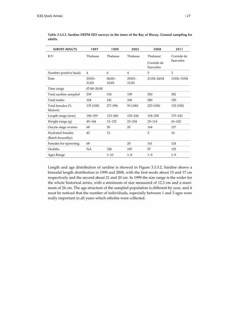
Table 3.3.3.3. Sardine DEPM IEO surveys in the inner of the Bay of Biscay. General sampling for adults.

SURVEY ADULTS 1997 1999 2002 2008 2011

R/V Thalassa Thalassa Thalassa Thalassa/

Cornide de Saavedra

Cornide de Saavedra

Number positive hauls 4 6 4 5 3

Date 29/03–31/03

06/03–10/03

29/03–31/03

21/04–24/04 13/04–15/04

Time range 07:00–20:00

Total sardine sampled 239 516 199 503 302

Total males 104 241 106 280 150

Total females (% Mature)

135 (100) 271 (98) 93 (100) 223 (100) 152 (100)

Length range (mm) 180–255 123–260 152–244 154–250 175–243

Weight range (g) 45–144 13–152 23–104 25–114 41–102

Oocyte stage ovaries 68 50 20 164 127

Hydrated females (Batch fecundity)

42 12 3 14

Females for spawning 68 20 161 124

Otoliths NA 328 195 97 129

Ages Range 1–10 1–8 1–9 1–9

Length and age distribution of sardine is showed in Figure 3.3.3.2. Sardine shows a bimodal length distribution in 1999 and 2008, with the first mode about 15 and 17 cm respectively and the second about 21 and 20 cm. In 1999 the size range is the wider for the whole historical series, with a minimum of size measured of 12.3 cm and a maxi-mum of 26 cm. The age structure of the sampled population is different by year, and it must be noticed that the number of individuals, especially between 1 and 3 ages were really important in all years which otholits were collected.


Figure 3.3.3.2. Sardine DEPM IEO surveys in the inner of the Bay of Biscay. Length (mm) and age distribution of sardine by year. No otoliths for age reading were available in 1997.

Final estimates of the mean female weight (W), batch fecundity (F), sex ratio (R), spawning frequency (S) and spawning–stock biomass (SSB) with their CVs are given in Table 3.3.3.4.

Table 3.3.3.4. Sardine DEPM IEO surveys in the inner of the Bay of Biscay. Summary of the results for eggs, adults and SSB estimates.

PARAMETER YEAR

Eggs 1997 1999 2002 2008 2011

Positive area (Km2) (%) 12 755(63) 5724(84) 9154(77) 8167(80) 12 400(88)

Z (hour-1)(CV%) -0.012(41) -0.006(89) -0.022(18) -0.019(26) -0.018(22)

P0 (eggs/m2/day)(CV%) 136.6(20) 78.7(13) 182.3(19) 171.4(23) 219.1(16)

P0 tot (eggs/day) (x1012) (CV%)

1.74(20) 0.45(13) 1.67(18) 1.4(23) 2.72(16)

Adults

Female Weight (g) (CV%) 74.5(11.8) 63.6(12.7) 62.9(5.6) 55.4(11.1) 61.3(9)

Batch Fecundity (CV%) 32 269(17) 32704(45) 24577 15849(29) 30 383(4)

Sex Ratio (CV%) 0.508(8.1) 0.535(10.7) 0.492(22.9) 0.483(8.9) 0.51(19.6)

Spawning Fraction (CV%) 0.131(9.7) 0.124(15.4) 0.143 0.137(24.4) 0.066(49.2)

Spawning Biomass (tons) (CV%)

60 332(31) 13 200(52) 60 720 73 942(47) 162 930(55)

The minimum mean weights by haul were observed in 1999 and the maximum 1997. Mean female weight (W) was similar for 1999, 2002 and 2011(63.6, 62.9 and 61.3, re-spectively) and considerably higher in 1997 (74.5). Mean females weights in 2008 sur-vey present the lowest value of the historical series (38.1). Concerning sex ratio estimates, mean values are quite homogeneous across the whole surveys.

Considering that few hydrated females (n=3) were collected in 2008 and no hydrated females were available in 1999 and 2002, the data from these three years were pooled

Age

020406080100

2 4 6 8 10

1997

020406080100

1999

020406080100

2002

020406080100

2005

020406080100

2008

020406080100

2011

Length (mm)

Num

ber

0

20

40

60

140 160 180 200 220 240

1997

0

20

40

60

1999

0

20

40

60

2002

0

20

40

60

2005

0

20

40

60

2008

0

20

40

60

2011


with data from North Atlantic Spanish coast, for the modelling of batch fecundity. Mean batch fecundity estimate (F) was considerably lower (15849 number of oocytes, 286 oocytes/gr) in 2008 according to the mean female weight estimated. On the contrary the first two surveys (1997 and 1999) presented the highest estimates (32 269, 433 oo-cytes/gr and 32 704, 514 oocytes/gr) of the historical series, though similar to the one obtained for the 2011(30 383, 495 oocytes/gr) survey. In particular, for 2002, although mean female weight was similar to the ones obtained during the 1999 and 2011 surveys, batch fecundity estimate was reduced to 24 577 (390 oocytes/gr) when compared to the values obtained these years.

Bootstrapped estimate of spawning fraction for 1999 was 0.124. Mean Spawning frac-tion estimate for 2011 survey was among the lowest (0.066) of the time-series. For the remaining surveyed years the values are generally quite high and homogeneous (be-tween 0.124 and 0.137).

SSB estimate

The whole survey-series DEPM-based SSB estimate is showed in Table 3.3.3.4. SSB in 2011 is the highest estimate of the time-series (162 930 tons), while 1999 is among the lowest of the time-series (13 200 tons). In 1997 and 2002 estimates are comparable (60 332 and 60 720 tons respectively) and in 2008 an increase in relation to the previous surveyed years was found (73 942 tons).

The lowest and highest SSB estimates found in 1999 and 2011 respectively are related to the egg production. Egg production estimate in the 1999 survey is the lowest of the time-series, probably due to the egg survey period has not covered the amount of spawning peak activity. By the contrary the large egg production estimate in 2011 is sustained by a combination of high egg production density (in eggs per day per square meter) and large spawning area. Moreover, the contribution of the lowest spawning fraction value (0.066) estimated in 2011 on the equation applied to estimate SSB, has largely increased the SSB value.

The estimates presented from DEPM application in the inner of the Bay of Biscay, are a priori considered provisionally. The way to obtain batch fecundity estimates for 1999, 2002 and 2008, modelling together with data from the North Atlantic Spanish coast, prevents to consider these preliminary results as definitely ones. Moreover, to solve the unreliable egg mortality estimated in 1999 an aggregated model similar to that used by Bernal et al., 2011, could be tried. All these issues require further analysis in terms of implications for the best estimation procedures and reliability of the results.

B.4. Commercial cpue

According to literature, cpue indices have been considered as not reliable indicators of abundance for small pelagic fishes (Ulltang, 1980; Csirke, 1988; Pitcher, 1995; Mackin-son et al., 1997). Commercial catch per unit of effort data are available at various levels of aggregation (subarea/gear/years) from official data, but these are not considered in-dicative of stock trends (see also information from the industry, below).

B.5. Other relevant data

Interviews with the French fishing industry operating in the Bay of Biscay highlighted a potential displacement of the stock further north. This could partly explain the in-crease of activity in the Celtic Sea over the last decade. According to fishermen, the main driver of the Bay of Biscay fishery is the market. Many fishers could catch more sardine as regards sardine availability, but this would not be suitable due to poor levels


of prices. Thus, the industry data should not directly be put in relation to variation of sardine abundance.

C. Assessment-data and method

From the modelling point of view, the lack of sampling, survey, biological information in the English Channel and Celtic Seas in contrast to the richness of the datasets avail-able for the Bay of Biscay does not allow the use of a single assessment method for the whole area. Therefore, for practical reasons related to the availability of data between the English Channel, Celtic Seas and Bay of Biscay, it was decided to divide this stock into two "data" regions: 8.a,b,d and 7..

The following indicators are considered relevant for the description of the stock in the different regions:

Subdivision 8.a,b,d

1 ) Trends in the Pelgas survey index; 2 ) Trends in the DEPM survey index.

Subdivision 7.

3 ) Trends in size (age?) distribution in catches (to be built up).

D. Short-term projection

No short-term projection method is currently set for this stock.

E. Medium-term projections

No medium-term projection method is currently set for this stock.

F. Long-term projections

No long-term projection method is currently set for this stock.

G. Biological reference points

No reference points are currently set for this stock. Given the differences of availability of data between the Celtic Seas, Bay of Biscay and English Channel, any set reference should take account of this or some regional reference points should be set accordingly.

Given the current lack of assessment, advices could be based on other indicators such as successive recruitment failure. These indicators are available from the current com-mercial and survey datasets.

H. Other issues

While the stock is considered to spread over Celtic Seas (7.a,b,c,f,j,k), Bay of Biscay (8.a,b,d) and English Channel (7.d,e,h), the critical lack of information in Celtic Seas and English Channel impairs the possibility of assessing this stock for the whole area.

H.1. Historical overview of previous assessment methods

2013 is the first year ICES is requested to give advice for sardine in 8.a,b,d and 7.. In previous years, exploratory assessments using TASACS were carried out during the working group on horse mackerel, anchovy and sardine (WGHANSA). Cohort track-ing analyses have also been conducted this year.


I. References Agresti, A. 1990. Categorical data analysis. John Wiley & Sons, Inc. New York.

Bernal, M., Borchers, D. L., Valde´s, L., Lago de Lanzo´ s, A., and Buckland, S. T. 2001. A new ageing method for eggs of fish species with daily spawning synchronicity. Canadian Journal of Fisheries and Aquatic Sciences, 58: 2330–2340.

Bernal, M., Ibaibarriaga, L., Lago de Lanzós, A., Lonergan, M., Hernández, C., Franco, C., Rasines, I., et al. 2008. Using multinomial models to analyse data fromsardine egg incubation experiments; a review of advances in fish egg incubation analysis techniques. ICES Journal of Marine Science, 65: 51–59.

Bernal M., Stratoudakis Y., Wood S., Ibaibarriaga L., Uriarte A., Valdés L., Borchers D. A revision of daily egg production estimation methods, with application to Atlanto-Iberian sardine. 1. Daily spawning synchronicity and estimates of egg mortality. ICES Journal of Marine Sci-ence 2011;68:519–527.

Binet D, Samb B, Sidi MT, Levenez JJ, Servain J. 1998. Sardine and other pelagic fisheries associ-ated with multi-year trade wind increases, pp. 212–233. Paris: ORSTOM.

Checkely D.M., Ortner P.B., Settle L.R., S.R. Cummings. 1997. A continuous, underway fish egg sampler. Fisheries Oceanography 6: 58–73.

Cochran, G. 1977. Sampling techniques, New York: Wiley and Sons.

Corten A, van de Kamp G. 1996. Variation in the abundance of southern fish species in the south-ern North Sea in relation to hydrography and wind. ICES J Mar. Sci. 53:1113–1119.

Csirke, J. 1988. Small shoaling pelagic fish stocks. In J.A. Gulland (Ed.). Fish population dynam-ics, pp. 271–302. 2nded. John Wiley & Sons, New York, 422 p.

Gamulin, T., and Hure, T. 1955. Contribution a la connaissance de l’ecologie de la ponte de la sardine, Sardina pilchardus (Walb.) dans l’Adriatique. Acta Adriatica, 70: 1–22.

Ganias, K., C. Nunes, and Y. Stratoudakis. 2007. Degeneration of postovulatory follicles in the Iberian sardine Sardina pilchardus: structural changes and factors affecting resorption. Fish. Bull. 105:131–139.

García, A., Pérez, N., Lo, N. C. H., Lago de Lanzos, A., and Sola, A. 1992. The Egg Production Method applied to the spawning biomass estimation of sardine, Sardina pil-chardus (Walb.) on the North Atlantic Spanish coast. Bo-letín del Instituto Español de Oceanografía, 8: 123–138.

Hunter, J.R. and Macewicz, B.J. 1985. Measurement of spawning frequency in multiple spawning fishes. In: An Egg Production Method for Estimating Spawning Biomass of Pelagic Fish: Application to the Northern Anchovy, Engraulis mordax (ed. R. Lasker ), NOAA Technical Report NMFS, US Department of Commerce, Springfield, VA, USA, 79–93.

Hunter, J. R., Lo, N. C. H., and Leong, J. H. 1985. Batch fecundity in multiple spawning fishes. In An Egg Produc-tion Method for Estimating Spawning Biomass of Pelagic Fish: Application to the Northern Anchovy, Engraulis mordax, pp. 67–77. Ed. by R. Lasker. NOAA Technical Report, NMFS 36.

Ibaibarriaga, L., Bernal, M., Motos, L., Uriarte, A., Borchers, D. L.,Lonergan, M., and Wood, S. 2007. Estimation of development properties of stage-classified biological processes using multinomial models: a case study of Bay of Biscay anchovy (Engraulis encrasicolus L.) egg development. Canadian Journal of Fisheries and Aquatic Sciences, 64: 539–553.

ICES. 2004. The DEPM estimation of spawning–stock biomass for sardine and anchovy. ICES Cooperative Research Report, 268. 91 pp.

ICES. WGACEGG. 2009. Report of the Working Group on Acoustic and Egg Surveys for Sardine and Anchovy in ICES Areas VIII and IX (WGACEGG), 16–20 November 2009, Lisbon, Por-tugal. ICES CM 2009/LRC:20. 181 pp.


ICES. WGACEGG. 2010. Report of the Working Group on Acoustic and Egg Surveys for Sardine and Anchovy in ICES Areas VIII and IX (WGACEGG), 22–26 November 2010. ICES CM 2010/SSGESST:24. 210 pp.

ICES. WGACEGG. 2011. Report of the Working Group on Acoustic and Egg Surveys for sardine and Anchovy in ICES Areas VIII and IX (WGACEGG), 21–25 November 2011, Barcelona, Spain. ICES CM 2011/SSGESST:20. 157 pp.

ICES. SGSBSA. 2002. Report of the Study Group on the estimation of spawning–stock biomass of sardine and anchovy. Lisbon, 22–25 October 2001. ICES CM 2002/G:01. 62 p.

ICES. 2011. Report of the workshop on Age reading of European Atlantic Sardine (WKARAS). ICES CM 2011/ACOM:42.91p.

ICES. 2012. Report of the Working Group on Southern Horse Mackerel, Anchovy and Sardine (WGHANSA), 23–28 June 2012, Azores (Horta), Portugal. ICES CM 2012/ACOM:16. 544pp.

ICES. 2016. Report of the Benchmark Workshop on Pelagic Stocks (WKPELA 2013), 4–8 February 2013, Copenhagen, Denmark. ICES CM 2013/ACOM:46.

Lasker, R. 1985. An Egg Production Method for Estimating Spawning Biomass of pelagic fish: Application to the Northern Anchovy, Engraulis mordax. NOAA Technical report NMFS 36:100p.

Lo, N.C.H. 1985a. A model for temperature-dependent northern anchovy egg development and an automated procedure for the assignment of age to staged eggs. In: An Egg Production Method for Estimating Spawning Biomass of Pelagic Fish: Application to the Northern An-chovy, Engraulis mordax (Ed. R. Lasker), NOAA Technical Report NMFS, US Department of Commerce, Springfield, VA, USA, 43–50.

Mackinson, S., Vasconcellos, M., Pitcher, T., and Walters, C. 1997. Ecosystem impacts of harvest-ing small pelagic fish in upwelling systems: using a dynamic mass-balance model. In Pro-ceedings of the Lowell Wakefield Symposium on Forage Fish in Marine Ecosystems, pp. 731–749. Alaska Sea Grant College Program, AS-SG-97-01.

Meynier, L. 2004. Food and feeding ecology of the common dolphin, Delphinus delphis in the Bay of Biscay: intra-specific dietary variation and food transfer modelling. MSc thesis, University of Aberdeen, Aberdeen, UK.

Motos, L. 1994. Estimación de la biomasa desovante de la población de anchoa del Golfo de Vizcaya Engraulis encrasicolus a partir de su producción de huevos. Bases metodológicas y aplicación. Ph. D. thesis UPV/EHU, Leioa.

Parker, K. 1980. A direct method for estimating northern anchovy, Engraulis mordax, spawning biomass. Fisheries. Bulletin., 78: 541–544.

Parrish RH, Serra R, Grant WS. 1989. The monotypic sardines, Sardina and Sardinops: their tax-onomy, stock structure, and zoogeography. Can. J. Fish. Aquat. Sci. 46: 2019–2036.

Pérez, N., Figueiredo, I., and Macewicz, B. J. 1992a. The spawning frequency of sardine, Sardina pilchardus (Walb.), off the Atlantic Iberian coast. Boletín del Institu-to Español de Oceano-grafía, 8: 175–189.

Pérez, N., Figueiredo, I., and Lo, N. C. H. 1992b. Batch fecundity of sardine, Sardina pilchardus (Walb.), off the Atlantic Iberian coast. Boletín del Instituto Español de Oceanografía, 8: 155–162 Petitgas et al.,2003.

Picquelle, S and G. Stauffer. 1985. Parameter estimation for an egg production method of an-chovy biomass assessment. In: R. Lasker (Ed.). An egg production method for estimating spawning biomass of pelagic fish: Application to the northern anchovy, Engraulis mordax, pp. 7–16. U.S. Dep. Commer.,NOAA Tech. Rep. NMFS 36.

Pitcher, T.J. 1995. The impact of pelagic fish behaviour on fisheries. Sci. Marina 59, pp. 295–306.

Santos, M.B, Pierce, G.J., López, A., Martínez, J.A., Fernández, M.T., Ieno, E., Mente, E., Porteiro, C., Carrera, P. and Meixide M. 2004. Variability in the diet of common dolphins (Delphinus


delphis) in Galician waters 1991–2003 and relationship with prey abundance. ICES CM 2004/Q:09.

Santos, A.M.P., Chícharo, A., Dos Santos, A., Miota, T., Oliveira, P.B., Peliz, A., and Ré, P. 2007. Physical-biological interactions in the life history of small pelagic fish in the Western Iberia Upwelling Ecosystem. Progress in Oceanography, 74: 192–209.

Santos M B, González-Quirós R, Riveiro I, Cabanas J M, Porteiro C, Pierce G J. 2011b. Cycles, trends, and residual variation in the Iberian sardine (Sardina pilchardus) recruitment series and their relationship with the environment. ICES Journal of Marine Science, doi:10.1093/icesjms/fsr186.

Sanz, A. and A. Uriarte. 1989. Reproductive cycle and batch fecundity of the Bay of Biscay an-chovy (Engraulis encrasicholus) in 1987. CalCOFI Rep., 30: 127–135.

Seber, G.A.F. The estimation of animal abundance and related parameters. Charles Griffin and Co., London, 2nd edition, 1982.

Silva, A. 2003. Morphometric variation among sardine (Sardina pilchardus) populations from the northeastern Atlantic and the western Mediterranean. ICES Journal of Marine Science, 60: 1352–1360.

Stratoudakis, Y., Coombs, S., Halliday, N., Conway, D., Smyth, T., Costas, G., Franco, C., Lago de Lanzo´ s, A., Bernal, M., Silva, A., Santos, M. B., Alvarez, P., and Santos, M. 2004. Sardine (Sardina pilchardus) spawning season in the North East Atlantic and relationships with sea surface temperature. ICES Document CM 2004/Q: 19. 19 pp.

Stratoudakis, Y., Bernal, M., Ganias, K., and Uriarte, A. 2006. The daily egg production methods: recent advances, current applications and future challenges. Fish and Fisheries, 7: 35–57.

Stauffer. G. D. and S J. Picquelle.1980. Estimates of the 1980 spawning biomass of the subpopu-lation of northern anchovy. Natl Mar Fish Sen, Southwest Fish Cent, La Jolla. CA. Admin Rep LJ-80.09. 41 p.

Ulltang, O. 1980. Factors effecting the reaction of pelagic fish stocks to exploitation and requiring a new approach to assessment and management. Rapport et P.V. des Reunions du Conseil International pour l’Exploration de la Mer, 177: 489–509.

stock annex: sardine (sardina pilchardus) in divisions 8.a ... reports/stock...

Documents