stock annex: sardine in division s 8abd

ICES WGHANSA REPORT 2019 | 1

Stock Annex: Sardine in divisions 8abd

Sardine (Sardina pilchardus) in divisions 8.a–b and 8.d (Bay of Biscay)

Stock specific documentation of standard assessment procedures used by ICES.

Stock Sardine

Working Group Working Group on Anchovy and Sardine and Southern Horse Mackerel (WGHANSA)

Created 25 February 2017(WKPELA)

Authors E. Duhamel, L. Citores, L. Ibaibarriaga, L. Pawlowski, I. Riveiro, M. Santos and A. Uriarte and the members of WKPELA 2017

Last updated 25 November 2019 (WGHANSA)

Last updated by E. Duhamel, L. Citores, L. Ibaibarriaga, L. Pawlowski, I. Riveiro, A. Uriarte

Sardine stock identity in divisions 8abd and Subarea 7 and approaches for assessment and management

European sardine (Sardine pilchardus Walbaum, 1792) has a wide distribution extend-ing in the Northeast Atlantic from the Celtic Sea and North Sea in the north to Mauri-tania in the south. Populations of Madeira, the Azores and the Canary Islands are at the western limit of the distribution (Parrish et al., 1989). Sardine is also found in the Mediterranean and the Black Seas. Changing environmental conditions affect sardine distribution, with fish having been found as far south as Senegal during episodes of low water temperature (Corten and van Kamp, 1996; Binet et al., 1998). Because of its continuous distribution in the Northeast Atlantic, it is likely that there is movement of fish between areas.

Microsatellite analyses revealed no significant genetic differentiation among sardines in Subareas 7 and 8 (Shaw et al., 2012). Recent genetic analyses conducted in the Celtic Seas and Western Channel show that no genetic differentiation has been detected be-tween the Bay of Biscay and Cornwall for the sardine stock (ICES, 2013). Therefore sardine in Celtic Seas (7.a,b,c,f,g,j,k), English Channel (7.d, 7.e, 7.h) and in Bay of Biscay (8.a,b,d) used to be considered to belong to the same stock from a genetic point of view. Therefore, it has been previously considered that the sardine stock in 8.a,b,d and 7.as a single stock unit. The assessment of this stock as a single unit has assumed that the trends derived from the observations made in the Bay of Biscay through the scientific surveys (PELGAS, Bioman) could be extended to the area 7.

Information from the ICES WKSAR workshop (ICES, 2016) suggests higher growth rates for the populations of the English Channel and Celtic sea than for the Bay of Bis-cay but it is unknown if this results from different oceanographic conditions or from population characteristics. Furthermore, there is no information on connectivity be-tween the Bay of Biscay and English Channel/Celtic Sea. Bordering catches in subarea 7 (statistical rectangles 25E4, 25E5) to the Bay of Biscay are generally considered to be taken from sardine populations in the Bay of Biscay. The recent PELTIC surveys (abun-dance of eggs, larvae, recruits and adults in the Channel) and results from the calorim-etry/growth analysis suggest that Channel/Celtic Sea can be a self-sustained

2 | ICES WGHANSA REPORT 2019

population. In fact, there are historical (Wallace and Pleasants, 1972) and recent evi-dences (Coombs et al., 2009) that a significant spawning takes place regularly in sub-area 7 and in a recent acoustic survey series in this area (Peltic surveys) relevant concentrations of all life stages (eggs, juveniles and adults) have been found as well (van der Kooij et al. Presentation to WKSAR report ICES CM 2016/ACOM:41). Further-more, the Cornish fisheries has been operating there for more than a century.

In terms of stock assessment, the availability of data strongly differs between the north-ern (Celtic Seas, English Channel) and the southern areas (Bay of Biscay). Additionally, each area presents different historical exploitation patterns. Therefore, analysis and management advice between the areas may differ.

The workshop concluded that in the absence of evidences of connectivity between the Bay of Biscay and Subarea 7 sardine populations, and taking into account the indica-tions of shelf sustained populations in each area (whereby all stages are found in sub-stantial amounts in both regions) it would be preferable to deal with the Bay of Biscay and Subarea 7 separately. Even in the case some connectivity would occur, dealing separately with them in a sustainable manner would be probably risk averse, as the potential northward emigrants from the Bay of Biscay to Subarea 7 would be com-prised in the natural mortality parameter estimated for the Bay of Biscay population.

For a better understanding of the Divisions within subareas 7 and 8 the ICES areas map can be seen below (Figure A.1.1).

Figure A.1.1. ICES Divisions in the Northeast Atlantic.


Fishery

There are currently no management measures implemented for this stock. The fisheries appear to be regulated by market price. Some fisheries (e.g. French fleets in the Bay of Biscay) have set their own local management in order to sustain correct market prices which imply targeting fish of certain sizes and limits to the total amount of catch.

An update of the French and Spanish catch data series in divisions 8.a and 8.b (from 1983 and 1996 for France and Spain, respectively) including 2015 catches was presented at WKPELA 2017. Spanish catches are taken by purse seines from the Basque Country operating mainly in Division 8.b. Spanish landings peaked in 1998 and 1999 with al-most 8 thousand tonnes but have until 2010 to below 1 thousand tons. In recent years (since 2011), the Spanish catches increased again, reaching 16 000 tons in 2014. The Spanish fishery takes place mainly between October and March. The strong increase of Spanish catches in 8.b is mainly due to an increase of the fishing effort, taking into account the low level of the Iberian sardine stock in 8c and some monthly closures of the southern fishery.

French catches have increased along the series, with values ranging from 4400 tonnes in 1983 to 23 000 tons in 2011 (Figure B.1.1). A total of 90% of the catches are taken by purse seiners while the remaining 10% is reported by pelagic trawlers (mainly pair trawlers). A substantial part of the French catches originates in divisions 7.h and 7.e, but these catches have been assigned to Division 8.a due to their very concentrated location at the boundary between 8.a, 7.h and 7.e.

When the ICES WGHANSA meeting was held in 2018, some substantial downward revision of the French catches had been done for 2016. Some investigations were car-ried out by Ifremer during the summer 2018, based on production data provided by the French fishing organisations. Some inconsistencies in catches were pointed out in some harbour on some quarter. It is unknown why the downward revision occurred in the official databases as data in WGHANSA 2017 had better matches with produc-tion data from the fishing organisations. Production data in 2016 were consistent with the official data used at WGHANSA 2017. Therefore, it was assumed that the produc-tion data reflected the actual catches and were included in the assessment with a revi-sion from 2013 to 2017. The revision has been applied since WGHANSA 2019.

Spanish catches were unusually high prior 1989 where a strong drop occurs. The rea-son of this drop is unknown but most likely related to some data area miss allocation issues which make any use of landings prior to this year uncertain.

For the French fleet, both purse seiners and pelagic trawlers target sardine in French waters. Average vessel length is about 18 m. Purse seiners operate mainly in coastal areas (<10 nautical miles) while trawlers are not allowed to fish within 3 nautical miles from the coast. Both pair trawlers and purse seiners operate close to their base harbour when targeting sardine. The highest catches are taken in the summer months. Almost all the catches are taken in southwest Brittany.

While French catches in divisions 8.a and 8.b are constituted by fish of a wide range of sizes with a peak at 20 cm length, sardine taken by Spanish vessels show a narrower range of sizes but with a peak at similar length size.


Figure B.1.1. Historical time-series of landings of sardine per country in the Bay of Biscay.

Ecosystem aspects

Sardine is prey of a range of fish and marine mammal species which take advantage of its schooling behaviour and availability. Sardine has been found to be important in the diet of common dolphins (Delphinus delphis) in Galicia (NW Spain) (Santos et al., 2004), Portugal (Silva, 2003) and the Atlantic French coast (Meynier, 2004). Recent studies of consumption of common dolphins in Galician (Santos et al., 2011) waters, give figures ranging from almost 6000 tons to more than 9000 tons of sardine, which represents a rather small proportion of the combined Spanish and Portuguese annual landings of sardine from ICES areas 8.c and 9.a (6–7%).There are also other species feeding on sar-dine, although to a lesser extent, such as: harbour porpoise (Phocoena phocoena), bottle-nose dolphin (Tursiops truncatus), striped dolphin (Stenella coeruleoalba), and white-sided dolphin (Lagenorhynchus acutus) (e.g. Santos et al., 2007).

Currently, no ecosystem driver has been considered in this assessment.

Data

Commercial catches

Landings data have been available for since 1950 on various aggregation levels. Data are considered to be accurate in the Bay of Biscay since 1989. Discards were measured only in 2012 and were low based on the French Observers at sea programme in the Bay of Biscay and hence not included in the assessment. In the past (late eighties and early nineties for the French Pelagic trawlers and sixties and seventies for the Spanish Purse seine fleet) they seemed to be more relevant (according to disputes among fishermen), but were never quantified. Bordering catches in Subarea 7 (statistical rectangles 25E4, 25E5) are considered belonging the Bay of Biscay area. Catches from those two statis-tical rectangles are therefore included in the total catches estimates used for the assess-ment.


Discards are considered negligible.

Biological

Catches-at-length and catches-at-age are known since 1984 for Spain and since 2002 for France in the Bay of Biscay. Because of the availability of the datasets, only the period starting in 2000 is used. They are obtained by applying to the monthly Length distri-butions half year or quarterly ALKs. Biological sampling of the catches has been gen-erally sufficient, and useful to have a better knowledge of the age structure of the catches. Complete age composition and mean weight-at-age on half-year basis, were yearly reported in ICES (WGHANSA report, ICES 2012).

Age reading is considered accurate. The most recent cross reading exchanges and workshop between Spain and France (but other countries, too) took place in 2011 (WKARAS report, ICES 2011). The overall level of agreement and precision in sardine of the Bay of Biscay age reading determinations seems to be satisfactory: Most of the sardine otoliths were well classified by most of the readers during the 2011 workshop (with an average agreement 75% and a CV of 14%).

Growth in weight and length are routinely obtained from surveys and from the moni-toring of the fishery. A declining trend in the weight and length-at-age has been ob-served throughout the series.

Maturity ogive is estimated every year since 2000 based on the PELGAS survey. Read-ings are considered accurate. Sardines mature in their first year of life. The proportion of mature individuals at a given age is declining through the time-series as a likely consequence of the decrease in length and weight. The current methodology considers all individuals of visual maturity stage 2 and beyond, are considered fully mature. In addition, maturity ogives can be obtained every three years from the adult sampling of the DEPM surveys.

Natural mortality are age-specific input values were deduced during WKPELA 2017 as the ones leading to the best fit of the observations in the assessment. This vector corresponds with values 90% of the Gislason’s expected M-at-age Vector-WKPELA2017 report):

Age 0 1 2 3 4 5 6+

M (year–1) 1.071 0.692 0.546 0.475 0.435 0.412 0.400

Surveys

Relevant surveys for the assessment are available for the Bay of Biscay only. Some sar-dines are caught during the various demersal surveys (e.g. FR-IBTS) occurring each year in the Celtic Seas, Bay of Biscay and English Channel but those catches are not substantial enough to be considered as indicators of the stock status.

The population present in the Bay of Biscay is monitored by the two surveys carried out in spring. On the one hand, the PELGAS acoustic surveys are conducted yearly and provide sardine estimates since 2000. On the other hand, BIOMAN DEPM surveys provide yearly a sardine egg abundance index since 1999, and every three years, to-gether with the SAREVA surveys, sardine spawning–stock biomass is estimated (since 2011).

This survey based monitoring system provides population estimates by the middle of the year, when a small part of the annual catches has been already taken.


Sardine acoustic indices (PELGAS survey)

Acoustic surveys are carried out every year in the Bay of Biscay in spring on board the French research vessel Thalassa since 2000. The objective of PELGAS surveys is to study the abundance and distribution of pelagic fish in the Bay of Biscay.

These surveys are connected with Ifremer programmes on data collection for monitor-ing and management of fisheries and ecosystemic approach for fisheries. This task is formally included in the first priorities defined by the Commission regulation EU N° 199/2008 of 06 November 2008 establishing the minimum and extended Commu-nity programmes for the collection of data in the fisheries sector, and laying down de-tailed rules for the application of Council Regulation (EC) No 1543/2000. These surveys must be considered in the frame of the Ifremer fisheries ecology action "resources var-iability" which is the French contribution to the international Globec programme. It is planned with Spain and Portugal in order to have most of the potential area to be cov-ered from Gibraltar to Brest (and Northern with the English survey PELTIC covering the Bristol Channel and the English waters of Western Channel since 2013) with the same sampling protocol. Data are available for the ICES working groups WGHANSA, WGWIDE and WGACEGG.

In 2003, survey data are considered less reliable because of unusual environmental conditions linked to the heat wave over Europe. Results this year were considered not representative of the true status of the stock.

PELGAS Method and sampling strategy

In the frame of an ecosystem approach, the pelagic ecosystem is characterised at each trophic level. In this objective, to assess an optimum horizontal and vertical description of the area, two types of actions are combined:

Continuous acquisition by storing acoustic data from three different echo-sounders (a multibean and multifrequency ME70, a singlebeam mul-tifrenquency ER60 and a singlebeam monofrequency lateral one)and pumping seawater under the surface in order to evaluate the number of fish eggs using a CUFES system (Continuous Under-water Fish Eggs Sampler);

Discrete sampling at stations (by trawls, plankton nets, CTD). Satellite imagery (temperature and sea colour) and modelisation will be also used before and during the cruise to recognise the main physical and biological structures and to improve the sampling strategy. Concurrently, a visual counting and identi-fication of cetaceans and birds (from board) is carried out in order to charac-terise the higher level predators of the pelagic ecosystem.

Satellite imagery (temperature and sea colour) and modelisation are also used before and during the cruise to recognise the main physical and biological structures and to improve the sampling strategy.

The strategy of the survey is the same for the whole series (since 2000).

Acoustic data were collected along systematic parallel transects perpendicular to the French coast (Figure B.3.3.1.1). The length of the ESDU (Elementary Sampling Distance Unit) was 1 mile and the transects were uniformly spaced by 12 nautical miles covering the continental shelf from 20 m depth to the shelf break.

Acoustic data were collected only during the day because of pelagic fish behaviour in this area. These species are usually dispersed very close to the surface during the night


and so "disappear" in the blind layer for the echo sounder between the surface and 8 m depth.

Two echo-sounders are usually used during surveys (SIMRAD EK60 for vertical echo-sounding and MARPORT on the pelagic trawl). Since 2009, the SIMRAD ME70 is used for multibeam visualisation. Energies and samples provided by split beam transducers (six frequencies EK60, 18, 38, 70, 120, 200 and 333 kHz), simple beam (MARPORT) and multibeam echo-sounder were simultaneously visualised, stored using the MOVIES+ software and at the same standard HAC format.

The calibration method is the same that the one described for the previous years (see WD 2001) with a tungsten sphere hanged up 20 m below the transducer and is gener-ally performed at anchorage in the Douarnenez Bay, on the west side of Brittany, dur-ing the very first day of the survey.

Acoustic data are collected by Thalassa along the totality of the daylight route from which about 2000 nautical miles on one way transect are usable for assessment. Fish are measured on board (for all species) and otoliths (for anchovy and sardine) are col-lected for age determinations.

Figure B.3.3.1.1. The acoustic transects network of the PELGAS survey.

Echoes scrutinizing

Most of the acoustic data along the transects are processed and scrutinised during the survey and are generally available one week after the end of the survey. Acoustic en-ergies (Sa) are cleaned by sorting only fish energies (excluding bottom echoes, para-sites, plankton, etc.) and classified into several categories of echo-traces according to the year fish (species) structures.

D1–energies attributed to mackerel, horse mackerel, blue whiting, and various demer-sal fish, corresponding to cloudy schools or layers (sometimes small dispersed points) close to the bottom or of small drops in a 10 m height layer close to the bottom.


D2–energies attributed to anchovy, sprat, sardine and herring corresponding to the usual echo-traces observed in this area since more than 15 years, constituted by schools well defined, mainly situated between the bottom and 50 meters above. These echoes are typical of clupeids in coastal areas and sometimes more offshore.

D3–energies attributed to blue whiting, myctophids and boarfish offshore, just closed to the shelf-break and on the platform in the north.

D4–energies attributed to sardine, mackerel and anchovy corresponding to small and dense echoes, very close to the surface.

D8–energies attributed exclusively to sardine (big and very dense schools).

Data processing

The global area is split into several strata where coherent communities are observed (species associations) in order to minimise the variability due to the variable mixing of species. For each stratum, a mean energy is calculated for each type of echoes and the area measured. A mean haul for the strata is calculated to get the proportion of species into the strata. This is obtained by estimating the average of species proportions weighted by the energy surrounding haul positions. Energies are therefore converted into biomass by applying catch ratio, length distributions and TS relationships. The calculation procedure for biomass estimate and variance is described in Petitgas et al., 2003.

The TS relationships used since 2000 are still the same and as following:

Sardine, anchovy & sprat: TS = 20 Log L – 71.2

Horse mackerel: TS = 20 Log L – 68.7

Blue whiting: TS = 20 Log L – 67.0

Mackerel: TS = 20 Log L – 86.0

The mean abundance per species in a stratum (tons m.n.-2) is calculated as:

),(),()( kDXkDskM eD

Ae ∑=

and total biomass (tons) by: )()( kMekABk

e ∑=

where,

k : strata index

D : echo type

e : species

SA: Average SA (NASC) in the strata (m2/n.mi.2)

Xe : species proportion coefficient (weighted by energy around each haul) (tons m-2)

A : area of the strata (m.n.2)

Then variance estimate is:

),(.)],(var[)(.)],([),()(. 22 kDesunkDsXkchankDXVarkDskMVar AeeD

Ae +=∑

)(.)(. 2 kMeVarkABVark

e ∑=


BeBeVarcv .= At the end, density in numbers and biomass by length and age are calculated for each species in each ESDU according to the nearest haul length composition. These numbers and biomass are weighted by the biomass in each stratum and data are used for spatial distributions by length and age.

The detailed protocol for these surveys (strategy and processing) is described in Annex 6 of WGACEGG report (ICES, 2009).

Sardine Daily Egg Production Method (BIOMAN-SAREVA Survey) and Egg Abundance Index

Collection of plankton samples and Egg abundance index and production estimates

Every year, the BIOMAN survey collects plankton samples in the southeast of the Bay of Biscay. Then, every three years, BIOMAN and SAREVA surveys are coordinated within WGACEGG to provide samples for the whole area. The annual coverage of the Bay of Biscay by Bioman is used to generate the Egg abundance index and the triennial coordinated surveys are used to implement the whole Daily Egg Production method to obtain biomass estimates.

In general, plankton samples in both surveys are obtained along a grid of parallel tran-sects perpendicular to the coast using a PairoVET equipped with 150 µm mesh net, until 100 m depth or 5 m to the bottom, (Pair of Vertical Egg Tow, Smith et al., 1985 in Lasker, 1985). Sardine, anchovy and other species eggs are sorted and counted. Since sampling is adaptive, the area represented by each station changes according to the sampling intensity and the survey limits.

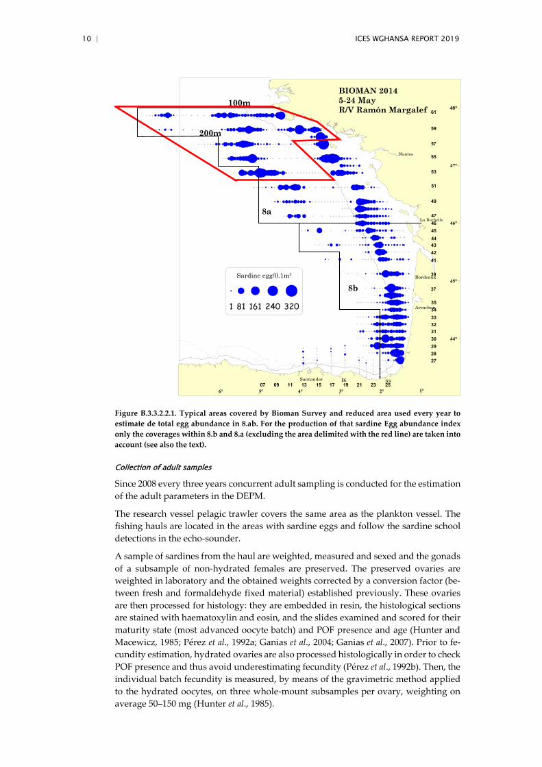
The Total sardine egg abundance index is obtained as the sum over the whole survey area of the product between the number of eggs found at each station and the area each station represents. This method (based on the total amount of sardine eggs in 8abd) is the one producing from BIOMAN the annual Egg abundance index used in the assess-ment. The standard area over which the Egg Abundance index is produced is pre-sented in Figure B3.3.2.2.1 (taking as example the survey in 2014), whereby coverages in 8.c and in the most northwestern area are removed (the latter because not every year the coverage of that northwest area is achieved). The few eggs in 8.c just close and continuing the spawning distribution from 8.b are always included within the index of Egg abundance for 8.abd.

For the application of the DEPM the egg abundances by stages and by samples are used to estimate the Daily Egg Production over the whole area following the proce-dures described below (in Section Total daily egg production estimates).

In these surveys, the Continuous Underway Fish Egg Sampler (CUFES, Checkley et al., 1997) is used as well to record the eggs found at 3–5 m depth with a net mesh size of 350 µm. Additional data, like oceanographic parameters, are also routinely obtained together with the plankton samples.


Figure B.3.3.2.2.1. Typical areas covered by Bioman Survey and reduced area used every year to estimate de total egg abundance in 8.ab. For the production of that sardine Egg abundance index only the coverages within 8.b and 8.a (excluding the area delimited with the red line) are taken into account (see also the text).

Collection of adult samples

Since 2008 every three years concurrent adult sampling is conducted for the estimation of the adult parameters in the DEPM.

The research vessel pelagic trawler covers the same area as the plankton vessel. The fishing hauls are located in the areas with sardine eggs and follow the sardine school detections in the echo-sounder.

A sample of sardines from the haul are weighted, measured and sexed and the gonads of a subsample of non-hydrated females are preserved. The preserved ovaries are weighted in laboratory and the obtained weights corrected by a conversion factor (be-tween fresh and formaldehyde fixed material) established previously. These ovaries are then processed for histology: they are embedded in resin, the histological sections are stained with haematoxylin and eosin, and the slides examined and scored for their maturity state (most advanced oocyte batch) and POF presence and age (Hunter and Macewicz, 1985; Pérez et al., 1992a; Ganias et al., 2004; Ganias et al., 2007). Prior to fe-cundity estimation, hydrated ovaries are also processed histologically in order to check POF presence and thus avoid underestimating fecundity (Pérez et al., 1992b). Then, the individual batch fecundity is measured, by means of the gravimetric method applied to the hydrated oocytes, on three whole-mount subsamples per ovary, weighting on average 50–150 mg (Hunter et al., 1985).

Sardine egg/0.1m²

1 81 161 240 320

200m

100m

282930

27

3132333435

37

39

41424344454647

49

51

53

2523211917151311Bi

Bordeaux

SS

Arcachon

Santander

Nantes

47°

46°

45°

44°

6° 5° 4° 3° 2° 1°

48°

La Rochelle

0907

55

57

59

61

BIOMAN 20145-24 MayR/V Ramón Margalef

8b

8a


Total daily egg production estimates

Every three years, the sardine eggs obtained jointly by the BIOMAN and SAREVA sur-veys are not only counted, but are further classified into eleven stages of development (adapted from Gamulin and Hure, 1955).

The total surveyed area is calculated as the sum of the area represented by each station and the spawning area is delimited with the outer zero sardine egg stations.

The eggs staged in the laboratory are transformed into daily cohort abundances using a multinomial model (Bayesian ageing method, Bernal et al., 2008). The Bayesian age-ing method requires a probability function of spawning time. Spawning time distribu-tion is assumed with a peak at 21:00 GMT. The upper age-cutting limit is the maximum age of unhatched eggs (at how. complete=0.99) for the whole strata corresponding with the percentile 95 of the incubation temperature of the eggs sampled in the strata, i.e. a value not dependent on the individual station. The lower age cutting excluded the first cohort of stations in which the sampling time is included within the daily spawning period.

Daily egg production (P0) and mortality (z) rates are estimated by fitting an exponential decay mortality model to the egg abundance by cohorts and corresponding mean age:

ageZePPE 0 ][ −=

The model is fitted as a generalized linear model (GLM) with negative binomial distri-bution and log link. Finally, the total egg production is calculated multiplying the daily egg production by the positive area.

+⋅= APPtot 0 The analysis is conducted in R (www.r-project.org) using the ”MASS” library for fitting the GLM and the libraries in http://sourceforge.net/projects/ichthyoanalysis/ for the egg ageing, calculation of the survey area and estimation of parameters.

Adult parameters, daily fecundity and SSB estimates

The adult parameters estimated for each fishing haul consider only the mature fraction of the population (determined by the fish macroscopic maturity data). Before the esti-mation of the mean female weight per haul (W), the individual total weight of the hy-drated females is corrected by a linear regression between the total weight of non-hydrated females and their corresponding gonad-free weight. The sex ratio (R) in weight per haul is obtained as the quotient between the total weight of females and the total weight of males and females. The expected individual batch fecundity (F)for all mature females (hydrated and non-hydrated) is estimated by the hydrated egg method (Hunter et al., 1985) i.e. by modelling the individual batch fecundity observed in the sample of hydrated females and their gonad free weight by a GLM and applying this subsequently to all mature females. The spawning fraction (S), the fraction of females spawning per day is determined for each haul, as the average number of females with Day-1 and Day-2 POF, divided by the total number of mature females. The hydrated females are not included due to possible oversampling of active spawning females close to the peak spawning time. In this case, the number of females with Day-0 POF (of the mature females) is corrected by the average number of females with Day-1 or Day-2 POF (Picquelle and Stauffer, 1985; Pérez et al., 1992a; Motos, 1994, Ganias et al., 2007).

http://www.r-project.org/

http://sourceforge.net/projects/ichthyoanalysis/


The mean and variance of the adult parameters for all the samples collected was then obtained using the methodology from Picquelle and Stauffer (1985) for cluster sam-pling (weighted means and variances).

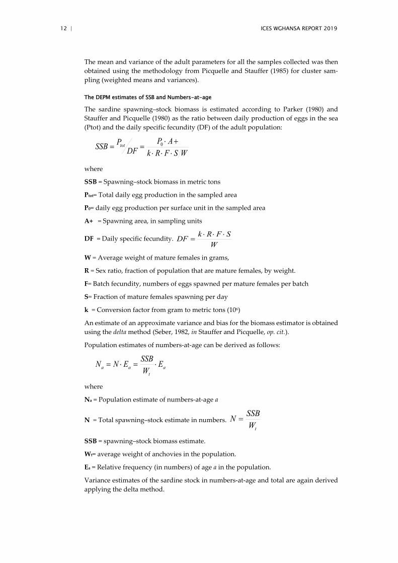
The DEPM estimates of SSB and Numbers-at-age

The sardine spawning–stock biomass is estimated according to Parker (1980) and Stauffer and Picquelle (1980) as the ratio between daily production of eggs in the sea (Ptot) and the daily specific fecundity (DF) of the adult population:

WSFRkAP

DFPSSB tot

⋅⋅⋅+⋅

== 0

where

SSB = Spawning–stock biomass in metric tons

Ptot= Total daily egg production in the sampled area

P0= daily egg production per surface unit in the sampled area

A+ = Spawning area, in sampling units

DF = Daily specific fecundity. W

SFRkDF ⋅⋅⋅=

W = Average weight of mature females in grams,

R = Sex ratio, fraction of population that are mature females, by weight.

F= Batch fecundity, numbers of eggs spawned per mature females per batch

S= Fraction of mature females spawning per day

k = Conversion factor from gram to metric tons (106)

An estimate of an approximate variance and bias for the biomass estimator is obtained using the delta method (Seber, 1982, in Stauffer and Picquelle, op. cit.).

Population estimates of numbers-at-age can be derived as follows:

at

aa EWSSBENN ⋅=⋅=

where

Na = Population estimate of numbers-at-age a

N = Total spawning–stock estimate in numbers. tW

SSBN =

SSB = spawning–stock biomass estimate.

Wt= average weight of anchovies in the population.

Ea = Relative frequency (in numbers) of age a in the population.

Variance estimates of the sardine stock in numbers-at-age and total are again derived applying the delta method.


Commercial cpue

According to literature, cpue indices have been considered as not reliable indicators of abundance for small pelagic fishes (Ulltang, 1980; Csirke, 1988; Pitcher, 1995; Mackin-son et al., 1997). Commercial catch per unit of effort data are available at various levels of aggregation (subarea/gear/years) from official data, but these are not considered in-dicative of stock trends (see also information from the industry, below).

Other relevant data

Interviews with the French fishing industry operating in the Bay of Biscay highlighted a potential displacement of the stock further north. This could partly explain the in-crease of activity in the Celtic Sea over the last decade. According to fishermen, the main driver of the Bay of Biscay fishery is the market. Many fishers could catch more sardine due to the high sardine availability, but this would not be suitable given the poor levels of prices. Thus, the industry data (landings) cannot be directly related to variations in sardine abundance.

Assessment-data and method

For the purposes of Assessment and Management the workshop concluded that in the absence of evidences of connectivity between the Bay of Biscay and Subarea 7 sardine populations, and taking into account the indications of shelf sustained populations in each area (whereby all stages are found in substantial amounts in both regions) it would be preferable to deal with the Bay of Biscay and Subarea 7 separately. Even in the case some connectivity would occur, dealing separately with the sardine in 8.abd and 7, in a sustainable manner, would be probably risk averse, as the potential north-ward emigrants from the Bay of Biscay to Subarea 7 would be comprised (assimilated) in the natural mortality parameter estimated for the Bay of Biscay population.

This assessment was considered by WKPELA2017 as indicative of trends only (laying it in category 2 stocks). Due to strong retrospective patterns, some investigations were carried out to improve the parameters settings of the model through the IBPsardine inter-benchmark in 2019. The retrospective patterns were strongly attenuated allowing the stock to be upgraded to category 1. The model now produces analytical estimates of biomass, recruitment and fishing pressure series, but the absolute levels are still lower than the surveys estimates.Estimated catchability for Pelgas biomass index (2.4), and for DEPM (1.8) have been perceived to be too high, because the acoustic and DEPM surveys are designed to estimate absolute biomass and because these catchabilities are quite different from those estimated for the southern sardine stock.


Assessment methods and settings

The data used for the assessment of sardine in divisions 8a,b,d are the following:

Type Name Year range Age range

Variable from year to year Yes/No

Caton Catch in tonnes 2000–onwards - Yes

Canum Catch-at-age in numbers

2002–onwards 0–6+ Yes

Weca Weight-at-age in the commercial catch


West Weight-at-age of the spawning stock at spawning time.


Mprop Proportion of natural mortality before spawning

2000–onwards 0–6+ No, equal to 0

Fprop Proportion of fishing mortality before spawning

2000–onwards 0–6+ No, equal to 0

Matprop Proportion mature at-age


Natmor Natural mortality at age

2000–onwards 0–6+ No

PELGAS acoustic survey

Biomass index and age structure

2000–onwards Yes

BIOMAN egg count

Egg count 2000–onwards Yes

DEPM SSB index 2011, 2014 Yes

Choice of stock assessment model

The model used is Stock Synthesis 3, version 3.24f (Methot, 2012). SS3 is a generalized age- and length-based model that is very flexible regarding the types of data that may be included, the functional forms that are used for various biological processes, the level of complexity and number of parameters that may be estimated. A description and discussion of the model can be found in Methot and Wetzel (2013).

Model used of basis for advice

The sardine assessment is an age-based assessment assuming a single area, a single fishery, a yearly season and genders combined. Input data include catch (in biomass), age composition of the catch, total abundance (in numbers) and age composition from an annual acoustic survey, total egg abundance and SSB from a triennial DEPM survey operating in the Bay of Biscay. Considering the current assessment calendar (annual assessment WG in June in year (y+1), the assessment includes fishery data up to year y and survey data up to year y+1. According to the ICES terminology, year y is the final year of the assessment and year y+1 is termed the interim year.


Assessment model configuration

The main model options are described below. A copy of the control file (sardine.ctl) including all model options is appended to the bottom of this Stock Annex.

Natural mortality are age-specific input values as listed in Section Ecosystem aspects.

Growth is not modelled explicitly. Weights-at-age and maturity-at-age at the begin-ning of the year are input values calculated using PELGAS survey data.

A Beverton–Holt stock–recruitment relationship, fixed steepness at 0.99, estimated es-timated sigmaR with Methot and Taylor bias correction.

Recruitment for the interim year of the assessment is assumed to be the historic geo-metric mean.

Fishing mortality is applied as the hybrid method. This method does a Pope’s approx-imation to provide initial values for iterative adjustment of the continuous F values to closely approximate the observed catch.

Total catch biomass by year is assumed to be accurate and precise. The F values are tuned to match this catch.

Both the acoustic survey, the total egg abundance index and the DEPM survey are as-sumed to be relative indices of abundance. The corresponding catchability coefficients are considered to be mean unbiased.

For DEPM and egg count surveys, selectivity is assumed to be fixed at 0 at age 0 and flat at 1 for ages 1 to 6+.

For Acoustic, selectivity was set to be flat between ages 2 and 6, with a value of 1 while selectivity for age 1. Age 6+ was estimated.

For the fishery selectivity, a flat shape was fixed for ages 3 to 6, with a value of 1, while for ages 1, 2 the selectivities were estimated.

Figure B.4.4.1. Selectivity-at-age for fisheries and surveys as estimated by WGHANSA2019.


The fishery selectivity is constant for the whole assessment period.

The model estimates population biomass in the beginning of the last assessment year (interim year). Data used for the interim year are the following: stock weights-at-age, catch biomass and catch weights-at-age are equal to those assumed for short-term pre-dictions (Section Short-term projection). The fishery age composition in the interim year is assumed to be equal to that in the previous year. The fishery age composition is included in the calculation of expected values, but excluded from the objective func-tion.

Initial estimates of data precision were as follows:

• Standard errors of biomass from PELGAS as estimated by the survey; • Standard error of 0.567 for DEPM SSB estimates; • Standard error of 0.448 for BIOMAN egg count index; • Sample size of PELGAS age structure: 40; • Sample size of fisheries age structure: 54.

Final model estimates were obtained after appropriate tuning of these values. Data precision values were changed iteratively until approximate convergence of the har-monic mean of expected sample size and the root mean squared error of the aggregated indices according to the model results.

• Indices of ageing imprecision is assumed to be constant for all ages and time: 0.1;

• The initial population is calculated by estimating an initial equilibrium pop-ulation modified by age composition data in the first year of the assessment (Methot and Wetzel, 2013). The initial equilibrium population was derived assuming an initial catch of 13 000 tons, the average of catches in 1990–1999.

Minimisation of the likelihood is implemented in phases using standard ADMB pro-cess. The phases in which estimation will begin for each parameter is shown in the control file appended to this section.

Variance estimates for all estimated parameters are calculated from the Hessian matrix.

The model estimates spawning–stock biomass (SSB) and summary biomass (B1+, bio-mass of age 1 and older) in the beginning of the year. The reference age range for out-put fishing mortality is 2–5 years.

Short-term projection

Model used: STF (fwd function from FLR Flash library)

Software used: FLR (Kell et al., 2007)

Initial stock size: the initial stock size corresponds to the assessment estimates for ages 1–6+ at the final year of the assessment.

Maturity: The maturity ogive is provided during the interim year by the PELGAS sur-vey.

F and M before spawning: Input values for the proportion of F and M before spawning are zero, which correspond to the beginning of the year when the SSB is estimated by the model.


Weight-at-age in the stock: Weights-at-age in the stock are provided during the interim year by the PELGAS survey.

Weight-at-age in the catch: Weights-at-age in the catch are calculated as the arithmetic mean value of the last three years of the assessment.

Exploitation pattern: The exploitation pattern is equal to the last year of the assessment.

Intermediate year assumptions: STF is set as catch constrained during the interim year. Preliminary catch are provided for quarter 1 to 3. Quarter 4 catches are estimated from the proportion of Q4 catches over total catches for the last three previous years of the assessment.

Stock–recruitment model used: Recruitment in the interim year and forecast year is set equal to the geometric mean of the time-series.

Medium-term projections

No medium-term projection method is currently set for this stock.

Long-term projections

No long-term projection method is currently set for this stock.

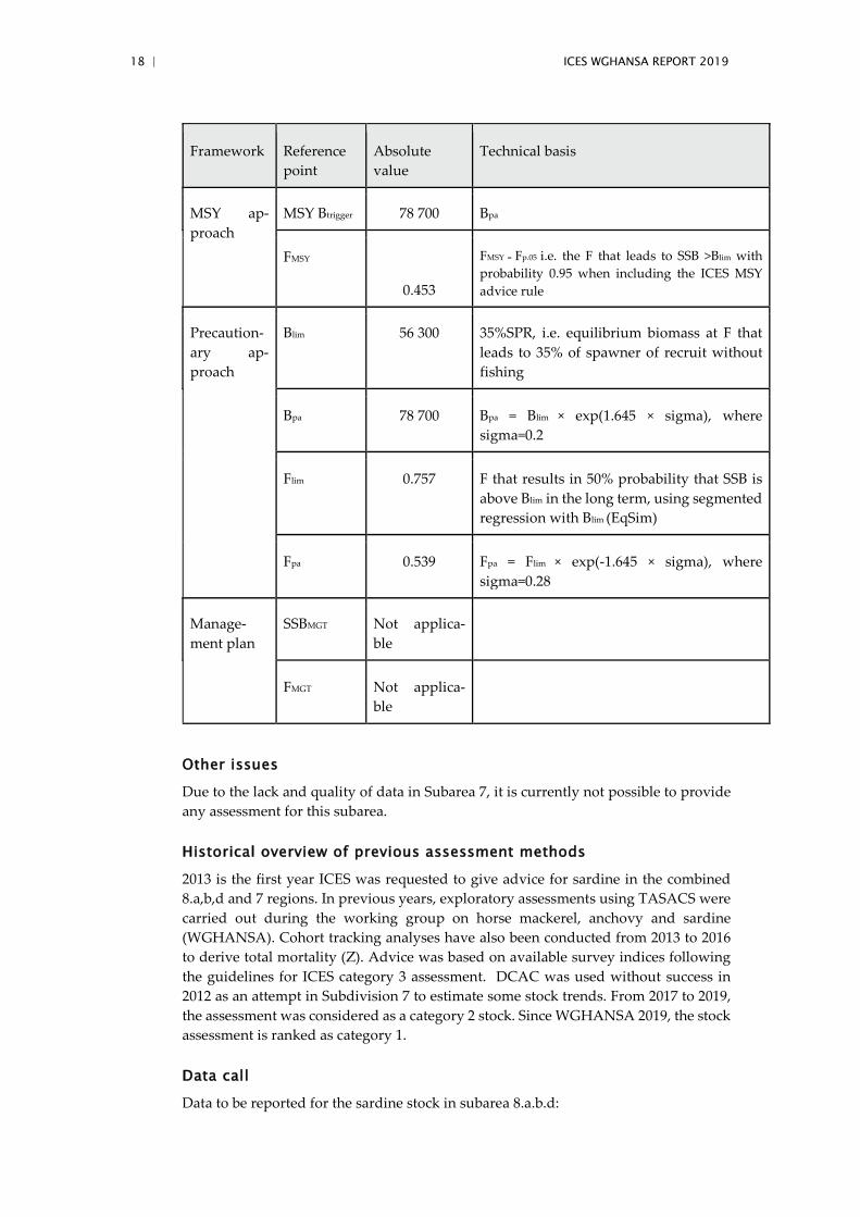
Biological reference points

Biological reference point were derived from the methodology set during the sardine inter-benchmark (ICES, 2019). It follows the ICES guideline to derive reference except Blim that serves as a starting point is not derived from Bloss but assumed to be 35%SPR, the equilibrium biomass at F that leads to 35% of spawner of recruit without fishing.


Framework Reference point

Absolute value

Technical basis

MSY ap-proach

MSY Btrigger 78 700 Bpa

FMSY

0.453

FMSY = Fp.05 i.e. the F that leads to SSB >Blim with probability 0.95 when including the ICES MSY advice rule

Precaution-ary ap-proach

Blim 56 300 35%SPR, i.e. equilibrium biomass at F that leads to 35% of spawner of recruit without fishing

Bpa 78 700 Bpa = Blim × exp(1.645 × sigma), where sigma=0.2

Flim 0.757 F that results in 50% probability that SSB is above Blim in the long term, using segmented regression with Blim (EqSim)

Fpa 0.539 Fpa = Flim × exp(-1.645 × sigma), where sigma=0.28

Manage-ment plan

SSBMGT Not applica-ble

FMGT Not applica-ble

Other issues

Due to the lack and quality of data in Subarea 7, it is currently not possible to provide any assessment for this subarea.

Historical overview of previous assessment methods

2013 is the first year ICES was requested to give advice for sardine in the combined 8.a,b,d and 7 regions. In previous years, exploratory assessments using TASACS were carried out during the working group on horse mackerel, anchovy and sardine (WGHANSA). Cohort tracking analyses have also been conducted from 2013 to 2016 to derive total mortality (Z). Advice was based on available survey indices following the guidelines for ICES category 3 assessment. DCAC was used without success in 2012 as an attempt in Subdivision 7 to estimate some stock trends. From 2017 to 2019, the assessment was considered as a category 2 stock. Since WGHANSA 2019, the stock assessment is ranked as category 1.

Data call

Data to be reported for the sardine stock in subarea 8.a.b.d:


1 ) Recent catch and biological data

France and Spain: time-series of length and age distribution of landings by quarter.

Other countries: catches in division 8.a.b.d. Time-series of length and age distribution when available.

2 ) Survey data

France: length distribution, numbers-at-age and weight-at-ages from the PELGAS sur-vey.

Spain: egg count and DEPM index from the BIOMAN survey.

References Agresti, A. 1990. Categorical data analysis. John Wiley & Sons, Inc. New York.

Ballón, M, Bertrand, B, Lebourges-Dhaussy, A, Gutiérrez, M, Ayón, P, Grados, D, and Gerlotto, F.2011. Is there enough zooplankton to feed forage fish populations off Peru? An acoustic (positive) answer. Progress in Oceanography 91, 2011, 360–381.

Bernal, M., Borchers, D. L., Valde´s, L., Lago de Lanzo´ s, A., and Buckland, S. T. 2001. A new ageing method for eggs of fish species with daily spawning synchronicity. Canadian Journal of Fisheries and Aquatic Sciences, 58: 2330–2340.

Bernal, M., Ibaibarriaga, L., Lago de Lanzós, A., Lonergan, M., Hernández, C., Franco, C., Rasines, I., et al. 2008. Using multinomial models to analyse data from sardine egg incuba-tion experiments; a review of advances in fish egg incubation analysis techniques. ICES Journal of Marine Science, 65: 51–59.

Bernal M., Stratoudakis Y., Wood S., Ibaibarriaga L., Uriarte A., Valdés L., Borchers D. 2011. A revision of daily egg production estimation methods, with application to Atlanto-Iberian sardine. 1. Daily spawning synchronicity and estimates of egg mortality. ICES Journal of Marine Science 2011: 68: 519–527.

Binet D, Samb B, Sidi MT, Levenez JJ, Servain J. 1998. Sardine and other pelagic fisheries associ-ated with multi-year trade wind increases, pp. 212–233. Paris: ORSTOM.

Checkely D.M., Ortner P.B., Settle L.R., S.R. Cummings. 1997. A continuous, underway fish egg sampler. Fisheries Oceanography 6: 58–73.

Coombs, S. H., Halliday, N. C., Conway, D. V. P., and Smyth, T. J. 2009. Sardine (Sardina pilchar-dus) egg abundance at station L4, Western English Channel, 1988–2008. J Plankton Res, 2010, 32 (5): 693–697. DOI: https://doi.org/10.1093/plankt/fbp052.

Cochran, G. 1977. Sampling techniques, New York: Wiley and Sons.

Corten A, van de Kamp G. 1996. Variation in the abundance of southern fish species in the south-ern North Sea in relation to hydrography and wind. ICES J Mar. Sci. 53:1113–1119.

Csirke, J. 1988. Small shoaling pelagic fish stocks. In J.A. Gulland (Ed.). Fish population dynam-ics, pp. 271–302. 2nded. John Wiley & Sons, New York, 422 pp.

Gamulin, T., and Hure, T. 1955. Contribution a la connaissance de l’ecologie de la ponte de la sardine, Sardina pilchardus (Walb.) dans l’Adriatique. Acta Adriatica, 70: 1–22.

Ganias, K., C. Nunes, and Y. Stratoudakis. 2007. Degeneration of postovulatory follicles in the Iberian sardine Sardina pilchardus: structural changes and factors affecting resorption. Fish. Bull. 105:131–139.

García, A., Pérez, N., Lo, N. C. H., Lago de Lanzos, A., and Sola, A. 1992. The Egg Production Method applied to the spawning biomass estimation of sardine, Sardina pilchardus (Walb.) on the North Atlantic Spanish coast. Boletín del Instituto Español de Oceanografía, 8: 123–138.


Hunter, J.R. and Macewicz, B.J. 1985. Measurement of spawning frequency in multiple spawning fishes. In: An Egg Production Method for Estimating Spawning Biomass of Pelagic Fish: Application to the Northern Anchovy, Engraulis mordax (ed. R. Lasker ), NOAA Technical Report NMFS, US Department of Commerce, Springfield, VA, USA, 79–93.

Hunter, J. R., Lo, N. C. H., and Leong, J. H. 1985. Batch fecundity in multiple spawning fishes. In An Egg Production Method for Estimating Spawning Biomass of Pelagic Fish: Application to the Northern Anchovy, Engraulis mordax, pp. 67–77. Ed. by R. Lasker. NOAA Technical Report, NMFS 36.

Ibaibarriaga, L., Bernal, M., Motos, L., Uriarte, A., Borchers, D. L.,Lonergan, M., and Wood, S. 2007. Estimation of development properties of stage-classified biological processes using multinomial models: a case study of Bay of Biscay anchovy (Engraulis encrasicolus L.) egg development. Canadian Journal of Fisheries and Aquatic Sciences, 64: 539–553.

ICES. 2004. The DEPM estimation of spawning–stock biomass for sardine and anchovy. ICES Cooperative Research Report, 268. 91 pp.

ICES. WGACEGG. 2009. Report of the Working Group on Acoustic and Egg Surveys for Sardine and Anchovy in ICES Areas VIII and IX (WGACEGG), 16–20 November 2009, Lisbon, Por-tugal. ICES CM 2009/LRC:20. 181 pp.

ICES. WGACEGG. 2010. Report of the Working Group on Acoustic and Egg Surveys for Sardine and Anchovy in ICES Areas VIII and IX (WGACEGG), 22–26 November 2010. ICES CM 2010/SSGESST:24. 210 pp.

ICES. WGACEGG. 2011. Report of the Working Group on Acoustic and Egg Surveys for sardine and Anchovy in ICES Areas VIII and IX (WGACEGG), 21–25 November 2011, Barcelona, Spain. ICES CM 2011/SSGESST:20. 157 pp.

ICES. SGSBSA. 2002. Report of the Study Group on the estimation of spawning–stock biomass of sardine and anchovy. Lisbon, 22–25 October 2001. ICES CM 2002/G:01. 62 pp.

ICES. 2011. Report of the workshop on Age reading of European Atlantic Sardine (WKARAS). ICES CM 2011/ACOM:42. 91 pp.

ICES. 2012. Report of the Working Group on Southern Horse Mackerel, Anchovy and Sardine (WGHANSA), 23–28 June 2012, Azores (Horta), Portugal. ICES CM 2012/ACOM:16. 544 pp.

ICES. 2019. Report of the Benchmark Workshop on Pelagic Stocks (WKPELA 2013), 4–8 February 2013, Copenhagen, Denmark. ICES CM 2013/ACOM:46.

ICES. 2019. Inter-benchmark process on sardine (Sardina pilchardus) in the Bay of Biscay (IBP-Sardine). ICES Scientific Reports. 1:80. 34 pp. http://doi.org/10.17895/ices.pub.5552.

Lasker, R. 1985. An Egg Production Method for Estimating Spawning Biomass of pelagic fish: Application to the Northern Anchovy, Engraulis mordax. NOAA Technical report NMFS 36:100 pp.

Lo, N.C.H. 1985a. A model for temperature-dependent northern anchovy egg development and an automated procedure for the assignment of age to staged eggs. In: An Egg Production Method for Estimating Spawning Biomass of Pelagic Fish: Application to the Northern An-chovy, Engraulis mordax (Ed. R. Lasker), NOAA Technical Report NMFS, US Department of Commerce, Springfield, VA, USA, 43–50.

Mackinson, S., Vasconcellos, M., Pitcher, T., and Walters, C. 1997. Ecosystem impacts of harvest-ing small pelagic fish in upwelling systems: using a dynamic mass-balance model. In Pro-ceedings of the Lowell Wakefield Symposium on Forage Fish in Marine Ecosystems, pp. 731–749. Alaska Sea Grant College Program, AS-SG-97-01.

Methot, R. M. 2012. User Manual for Stock Synthesis. Seattle, WA: NOAA Fisheries.

Methot R. D., Wetzel C. R. 2013. Stock synthesis: a biological and statistical framework for fish stock assessment and fishery management. Fisheries Research, 142:86–99.


Meynier, L. 2004. Food and feeding ecology of the common dolphin, Delphinus delphis in the Bay of Biscay: intra-specific dietary variation and food transfer modelling. MSc thesis, Univer-sity of Aberdeen, Aberdeen, UK.

Motos, L. 1994. Estimación de la biomasa desovante de la población de anchoa del Golfo de Viz-caya Engraulis encrasicolus a partir de su producción de huevos. Bases metodológicas y aplicación. PhD thesis UPV/EHU, Leioa.

Parker, K. 1980. A direct method for estimating northern anchovy, Engraulis mordax, spawning biomass. Fisheries Bulletin. 78: 541–544.

Parrish RH, Serra R, Grant WS. 1989. The monotypic sardines, Sardina and Sardinops: their tax-onomy, stock structure, and zoogeography. Can. J. Fish. Aquat. Sci. 46: 2019–2036.

Pérez, N., Figueiredo, I., and Macewicz, B. J. 1992a. The spawning frequency of sardine, Sardina pilchardus (Walb.), off the Atlantic Iberian coast. Boletín del Instituto Español de Oceanogra-fía, 8: 175–189.

Pérez, N., Figueiredo, I., and Lo, N. C. H. 1992b. Batch fecundity of sardine, Sardina pilchardus (Walb.), off the Atlantic Iberian coast. Boletín del Instituto Español de Oceanografía, 8: 155–162 Petitgas et al., 2003.

Picquelle, S and G. Stauffer. 1985. Parameter estimation for an egg production method of an-chovy biomass assessment. In: R. Lasker (Ed.). An egg production method for estimating spawning biomass of pelagic fish: Application to the northern anchovy, Engraulis mordax, pp. 7–16. U.S. Dep. Commer. NOAA Tech. Rep. NMFS 36.

Pitcher, T.J. 1995. The impact of pelagic fish behaviour on fisheries. Sci. Marina 59, pp. 295–306.

Santos, M.B, Pierce, G.J., López, A., Martínez, J.A., Fernández, M.T., Ieno, E., Mente, E., Porteiro, C., Carrera, P. and Meixide M. 2004. Variability in the diet of common dolphins (Delphinus delphis) in Galician waters 1991–2003 and relationship with prey abundance. ICES CM 2004/Q: 09.

Santos, A.M.P., Chícharo, A., Dos Santos, A., Miota, T., Oliveira, P.B., Peliz, A., and Ré, P. 2007. Physical-biological interactions in the life history of small pelagic fish in the Western Iberia Upwelling Ecosystem. Progress in Oceanography, 74: 192–209.

Santos M.B, González-Quirós R, Riveiro I, Cabanas J M, Porteiro C, Pierce G J. 2011b. Cycles, trends, and residual variation in the Iberian sardine (Sardina pilchardus) recruitment series and their relationship with the environment. ICES Journal of Marine Science, doi:10.1093/icesjms/fsr186.

Sanz, A. and A. Uriarte. 1989. Reproductive cycle and batch fecundity of the Bay of Biscay an-chovy (Engraulis encrasicholus) in 1987. CalCOFI Rep., 30: 127–135.

Seber, G.A.F. 1982. The estimation of animal abundance and related parameters. Charles Griffin and Co., London, 2nd edition, 1982.

Silva, A. 2003. Morphometric variation among sardine (Sardina pilchardus) populations from the Northeastern Atlantic and the western Mediterranean. ICES Journal of Marine Science, 60: 1352–1360.

Stratoudakis, Y., Coombs, S., Halliday, N., Conway, D., Smyth, T., Costas, G., Franco, C., Lago de Lanzo´ s, A., Bernal, M., Silva, A., Santos, M. B., Alvarez, P., and Santos, M. 2004. Sardine (Sardina pilchardus) spawning season in the North East Atlantic and relationships with sea surface temperature. ICES Document CM 2004/Q: 19. 19 pp.

Stratoudakis, Y., Bernal, M., Ganias, K., and Uriarte, A. 2006. The daily egg production methods: recent advances, current applications and future challenges. Fish and Fisheries, 7: 35–57.

Stauffer, G. D. and S. J. Picquelle. 1980. Estimates of the 1980 spawning biomass of the subpop-ulation of northern anchovy. Natl Mar Fish Sen, Southwest Fish Cent, La Jolla. CA. Admin Rep LJ-80.09. 41 pp.


Ulltang, O. 1980. Factors effecting the reaction of pelagic fish stocks to exploitation and requiring a new approach to assessment and management. Rapport et P.V. des Reunions du Conseil International pour l’Exploration de la Mer, 177: 489–509.

Wallace, P.D. and Pleasants. C.A. 1972. The distribution of eggs and larvae of some pelagic fish species in the English Channel and adjacent waters in 1967 and 1968. ICES CM. 1972/J: 8, 17 pp. (mimeo).


Appendix: Control file for sardine assessment in Bay of Biscay (8.a.b.d) only

#C Sardine in VIIIc and IXa : SPALY 2016

#C growth parameters are estimated spawner-recruitment bias adjustment Not tuned For optimality

#_data_and_control_files: sardine.dat // sardine.ctl

1 #_N_Growth_Patterns

1 #_N_Morphs_Within_GrowthPattern

#_Cond 1 #_Morph_between/within_stdev_ratio (no read if N_morphs=1)

#_Cond 1 #vector_Morphdist_(-1_in_first_val_gives_normal_approx)

#

#_Cond 0 # N recruitment designs goes here if N_GP*nseas*area>1

#_Cond 0 # placeholder for recruitment interaction request

#_Cond 1 1 1 # example recruitment design element for GP=1, seas=1, area=1

#

#_Cond 0 # N_movement_definitions goes here if N_areas > 1

#_Cond 1.0 # first age that moves (real age at begin of season, not integer) also cond on do_migration>0

#_Cond 1 1 1 2 4 10 # example move definition for seas=1, morph=1, source=1 dest=2, age1=4, age2=10

#

0 #_Nblock_Patterns

# 1 #_blocks_per_pattern

# begin and end years of blocks

# 1983 1990

#

0.5 #_fracfemale

3 #_natM_type:_0=1Parm; 1=N_breakpoints;_2=Lorenzen;_3=agespecific;_4=agespec_withseasinterpolate

1.0710 0.6912 0.5463 0.4752 0.4356 0.4122 0.3978 #_no additional input for selected M option; read 1P per morph

1 # GrowthModel: 1=vonBert with L1&L2; 2=Richards with L1&L2; 3=age_speciific_K; 4=not implemented

1 #_Growth_Age_for_L1

6 #_Growth_Age_for_L2 (999 to use as Linf)

0 #_SD_add_to_LAA (set to 0.1 for SS2 V1.x compatibility)

0 #_CV_Growth_Pattern: 0 CV=f(LAA); 1 CV=F(A); 2 SD=F(LAA); 3 SD=F(A); 4 logSD=F(A)


5 #_maturity_option: 1=length logistic; 2=age logistic; 3=read age-maturity matrix by growth_pattern; 4=read age-fecundity; 5=read fec and wt from wtatage.ss

#_placeholder for empirical age-maturity by growth pattern

1 #_First_Mature_Age

1 #_fecundity option:(1)eggs=Wt*(a+b*Wt);(2)eggs=a*L^b;(3)eggs=a*Wt^b; (4)eggs=a+b*L; (5)eggs=a+b*W

0 #_hermaphroditism option: 0=none; 1=age-specific fxn

1 #_parameter_offset_approach (1=none, 2= M, G, CV_G as offset from female-GP1, 3=like SS2 V1.x)

2 #_env/block/dev_adjust_method (1=standard; 2=logistic transform keeps in base parm bounds; 3=standard w/ no bound check)

#

#_growth_parms

#_LO HI INIT PRIOR PR_type SD PHASE env-var use_dev dev_minyr dev_maxyr dev_stddev Block Block_Fxn

6 17 13 0 -1 0 -2 0 0 0 0 0 0 0 # L_at_Amin_Fem_GP_1

19 28 23 0 -1 0 -4 0 0 0 0 0 0 0 # L_at_Amax_Fem_GP_1

0.2 0.8 0.4 0 -1 0 -4 0 0 0 0 0 0 0 # VonBert_K_Fem_GP_1

0.05 0.25 0.1 0 -1 0 -3 0 0 0 0 0 0 0 # CV_young_Fem_GP_1

0.05 0.25 0.1 0 -1 0 -3 0 0 0 0 0 0 0 # CV_old_Fem_GP_1

-3 3 2 0 -1 0 -3 0 0 0 0 0 0 0 # Wtlen_1_Fem

-3 4 3 0 -1 0 -3 0 0 0 0 0 0 0 # Wtlen_2_Fem

50 60 55 0 -1 0 -3 0 0 0 0 0 0 0 # Mat50%_Fem

-3 3 -0.25 0 -1 0 -3 0 0 0 0 0 0 0 # Mat_slope_Fem

-3 3 1 0 -1 0 -3 0 0 0 0 0 0 0 # Eggs/kg_inter_Fem

-3 3 0 0 -1 0 -3 0 0 0 0 0 0 0 # Eggs/kg_slope_wt_Fem

0 0 0 0 -1 0 -4 0 0 0 0 0 0 0 # RecrDist_GP_1

0 0 0 0 -1 0 -4 0 0 0 0 0 0 0 # RecrDist_Area_1

0 0 0 0 -1 0 -4 0 0 0 0 0 0 0 # RecrDist_Seas_1

0 0 0 0 -1 0 -4 0 0 0 0 0 0 0 # CohortGrowDev

#

#_Cond 0 #custom_MG-env_setup (0/1)

#_Cond -2 2 0 0 -1 99 -2 #_placeholder when no MG-environ parameters

#

#_Cond 0 #custom_MG-block_setup (0/1)

#_Cond -2 2 0 0 -1 99 -2 #_placeholder when no MG-block parameters

#_Cond No MG parm trends


#

#_seasonal_effects_on_biology_parms

0 0 0 0 0 0 0 0 0 0 #_femwtlen1,femwtlen2,mat1,mat2,fec1,fec2,Malewtlen1,malewtlen2,L1,K

#_Cond -2 2 0 0 -1 99 -2 #_placeholder when no seasonal MG parameters

#

#_Cond -4 #_MGparm_Dev_Phase

#

#_Spawner-Recruitment

3 #_SR_function: 2=Ricker; 3=std_B-H; 4=SCAA; 5=Hockey; 6=B-H_flattop; 7=survival_3Parm

#_LO HI INIT PRIOR PR_type SD PHASE

1 12 8.9 4.5 -1 5 1 # SR_LN(R0)

0.2 1 0.99 0.7 -1 0.05 -5 # Steepness

0.2 4 0.55 0.6 -1 0.8 4 # SR_sigmaR

-5 5 0.1 0 -1 1 -3 # SR_envlink

-5 5 0 0 -1 1 -4 # SR_R1_offset

0 0 0 0 -1 0 -99 # SR_autocorr

0 #_SR_env_link

0 #_SR_env_target_0=none;1=devs;_2=R0;_3=steepness

1 #do_recdev: 0=none; 1=devvector; 2=simple deviations

1996 # first year of main recr_devs; early devs can preceed this era

2018 # last year of main recr_devs; forecast devs start in following year

2 #_recdev phase

1 # (0/1) to read 13 advanced options

0 #_recdev_early_start (0=none; neg value makes relative to recdev_start)

-4 #_recdev_early_phase

-1 #_forecast_recruitment phase (incl. late recr) (0 value resets to maxphase+1)

1 #_lambda for Fcast_recr_like occurring before endyr+1

1985.3 #_last_early_yr_nobias_adj_in_MPD

1998.7 #_first_yr_fullbias_adj_in_MPD

2017.8 #_last_yr_fullbias_adj_in_MPD

2019.7 #_first_recent_yr_nobias_adj_in_MPD

0.9466 #_max_bias_adj_in_MPD (1.0 to mimic pre-2009 models)

0 #_period of cycles in recruitment (N parms read below)

-5 #min rec_dev


5 #max rec_dev

0 #_read_recdevs

#_end of advanced SR options

#

#_placeholder for full parameter lines for recruitment cycles

# read specified recr devs

#_Yr Input_value

#

# all recruitment deviations

#Fishing Mortality info

0.3 # F ballpark for tuning early phases

-2001 # F ballpark year (neg value to disable)

3 # F_Method: 1=Pope; 2=instan. F; 3=hybrid (hybrid is recommended)

2 # max F or harvest rate, depends on F_Method

# no additional F input needed for Fmethod 1

# if Fmethod=2; read overall start F value; overall phase; N detailed inputs to read

# if Fmethod=3; read N iterations for tuning for Fmethod 3

4 # N iterations for tuning F in hybrid method (recommend 3 to 7)

#

#_initial_F_parms

#_LO HI INIT PRIOR PR_type SD PHASE

0 2 0.3 0.3 -1 0.2 1 # InitF_1purse_seine

#

#_Q_setup

# Q_type options: <0=mirror, 0=median_float, 1=mean_float, 2=parameter, 3=parm_w_random_dev, 4=parm_w_randwalk, 5=mean_unbiased_float_assign_to_parm

#_for_env-var:_enter_index_of_the_env-var_to_be_linked

#_Den-dep env-var extra_se Q_type

0 0 0 0 # 1 purse_seine

0 0 0 2 # 2 Acoustic_survey

0 0 0 2 # 3 egg_survey

0 0 0 2 # 4 Depm_survey

#

#_Cond 0 #_If q has random component, then 0=read one parm for each fleet with random q; 1=read a parm for each year of index

#_Q_parms(if_any)


# LO HI INIT PRIOR PR_type SD PHASE

-7 5 0 0 -1 0.5 1 # Q_base_2_biomass_survey

-7 5 0 2 -1 2 1 # Q_base_3_egg_survey

-7 5 0 0 -1 0.5 1 # Q_base_4_depm

#

#_size_selex_types

#_Pattern Discard Male Special



30 0 0 0 # 3 egg_survey


#

#_age_selex_types

#_Pattern ___ Male Special



10 0 0 0 # 3 egg_survey


#_LO HI INIT PRIOR PR_type SD PHASE env-var use_dev dev_minyr dev_maxyr dev_stddev Block Block_Fxn

-999 -999 -999 -6 -1 0.1 -2 0 3 0 0 0.1 0 0 # AgeSel_1P_1_purse_seine

-5 9 0 0 -1 0.1 1 0 0 0 0 0.1 0 0 # AgeSel_1P_2_purse_seine

-5 9 0 0 -1 0.1 1 0 0 0 0 0.1 0 0 # AgeSel_1P_3_purse_seine

-0.01 9 0 0 -1 0.1 1 0 0 0 0 0.1 0 0 # AgeSel_1P_4_purse_seine

-5 0 0 0 -1 0.1 -1 0 0 0 0 0.1 0 0 # AgeSel_1P_5_purse_seine




-1000 -1000 -1000 -6 -1 0.1 -2 0 0 0 0 0 0 0 # AgeSel_2P_1_Acoustic_survey

-5 5 0 0 -1 0.1 1 0 0 0 0 0 0 0 # AgeSel_2P_2_Acoustic_survey

-0.01 9 0 0 -1 0.1 1 0 0 0 0 0 0 0 # AgeSel_2P_3_Acoustic_survey

-5 0 0 0 -1 0.1 -1 0 0 0 0 0 0 0 # AgeSel_2P_4_Acoustic_survey




#_Cond 0 #_custom_sel-env_setup (0/1)

#_Cond -2 2 0 0 -1 99 -2 #_placeholder when no enviro fxns

# #_custom_sel-blk_setup (0/1)

#_Cond No selex parm trends

4 #_selparmdev-phase

1 #_env/block/dev_adjust_method (1=standard; 2=logistic trans to keep in base parm bounds; 3=standard w/ no bound check)

#

# Tag loss and Tag reporting parameters go next

0 # TG_custom: 0=no read; 1=read if tags exist

#_Cond -6 6 1 1 2 0.01 -4 0 0 0 0 0 0 0 #_placeholder if no parameters

#

1 #_Variance_adjustments_to_input_values

#_fleet: 1 2 3 4

0 0 0 0 #_add_to_survey_CV

0 0 0 0 #_add_to_discard_stddev

0 0 0 0 #_add_to_bodywt_CV

0 0 0 0 #_mult_by_lencomp_N

1 1 1 1 #_mult_by_agecomp_N

1 1 1 1 #_mult_by_size-at-age_N

#

4 #_maxlambdaphase

1 #_sd_offset


#

4 # number of changes to make to default Lambdas (default value is 1.0)

# Like_comp codes: 1=surv; 2=disc; 3=mnwt; 4=length; 5=age; 6=SizeFreq; 7=sizeage; 8=catch;

# 9=init_equ_catch; 10=recrdev; 11=parm_prior; 12=parm_dev; 13=CrashPen; 14=Morphcomp; 15=Tag-comp; 16=Tag-negbin

#like_comp fleet/survey phase value sizefreq_method

9 1 1 1 1

4 2 2 1 1

4 2 3 1 1

4 2 4 1 1

#

# lambdas (for info only; columns are phases)

# 0 0 0 0 #_CPUE/survey:_1

# 1 1 1 1 #_CPUE/survey:_2

# 1 1 1 1 #_CPUE/survey:_3

# 1 1 1 1 #_agecomp:_1

# 1 1 1 1 #_agecomp:_2

# 0 0 0 0 #_agecomp:_3

# 1 1 1 1 #_init_equ_catch

# 1 1 1 1 #_recruitments

# 1 1 1 1 #_parameter-priors

# 1 1 1 1 #_parameter-dev-vectors

# 1 1 1 1 #_crashPenLambda

0 # (0/1) read specs for more stddev reporting

#0 2 -1 7 0 7 -1 2018 6 # placeholder for selex type, len/age, year, N selex bins, Growth pattern, N growth ages, NatAge_area(-1 for all), NatAge_yr, N Natages

#5 16 27 38 46 0 0 # vector with selex std bin picks (-1 in first bin to self-generate)

#1 2 14 26 40 0 0 # vector with growth std bin picks (-1 in first bin to self-generate)

#1 2 3 4 5 6 # vector with N-at-age std bin picks (-1 in first bin to self-generate)

999

stock annex: sardine in division s 8abd

Documents