1

Southern California Aerial Survey for Pacific Sardine (Sardinops sagax) and Northern Anchovy (Engraulis mordax)

Kirk Lynn1, Dianna Porzio, Trung Nguyen, Laura Ryley

California Department of Fish and Wildlife

8901 La Jolla Shores Drive1 La Jolla, CA 92037

EXECUTIVE SUMMARY

The Southern California Coastal Pelagic Species Survey (SCCPSS) is a joint aerial survey between the California Department of Fish and Wildlife (CDFW) and the California Wetfish Producers Association (CWPA) that provides data on nearshore abundance of Pacific sardine (Sardinops sagax) and northern anchovy (Engraulis mordax). Information used for management of these commercially valuable stocks is largely provided by research methods that do not adequately sample nearshore areas where significant biomass has been observed. The SCCPSS conducts daytime visual surveys biannually over waters of the Southern California Bight (SCB) in coastal areas of the mainland and the islands.

The SCCPSS proposes two projects that can inform sardine and anchovy stock assessments. Survey data collected since 2012 are applied to Project 1, a nearshore index of relative abundance based on density, defined as observed tons per area surveyed. Initiated in September 2016, Project 2 provides an inshore correction factor for the acoustic-trawl method (ATM) survey to account for nearshore areas not surveyed by ships due to operational constraints. In addition, boat sampling is conducted simultaneously with aerial observers to validate species identifications and obtain biological data from collected samples.

Survey results show decreases in observed biomass and density for both sardine and anchovy between 2012-2013 and 2015, with some signs of increase for both in 2016. Data collected to date for Project 2 have not been sufficient to calculate an inshore correction factor, as fish of the same species were not observed in both offshore and inshore areas. Boat sampling has shown strong survey observer accuracy in species identification, and has produced limited biological information.

Project 1 data from the SCCPSS can be used as an index of relative abundance, or as an estimate of nearshore minimum absolute abundance to be combined with ATM estimates. If sufficient data across area and replication are collected for Project 2, the results can be used to determine nearshore biomass and, combined with ATM estimates, produce a minimum estimate of abundance for the SCB area. Biological sampling can be enhanced and timed with aircraft and ship surveys to complement indices of abundance. Boat sampling efforts will continue with attempts to expand the range of operations and to improve sampling efficiency with trawl nets, which will help inform selectivity for integrated stock assessment models.

Agenda Item D.2.aCDFW Report

June 2017

2

Results from this survey are subject to several assumptions associated with the methods employed. Fish that are detectable from this method are assumed to be representative of the stock. Further studies can provide information on depth distribution and behavioral characteristics such as vertical and latitudinal movements, as well as environmental conditions affecting these patterns. Weather significantly impacts survey operations with unknown effects on the timing and location of transects. Use of habitat models to apportion results to the correct subpopulation of sardine is also an important consideration.

[Note: Project 2 was evaluated and not recommended by the review panel as a viable method for calculating nearshore abundance. For the purposes of this report, it will be described as it was presented at the review meeting.]

INTRODUCTION

The current stock assessment methods for coastal pelagic species (CPS) managed by the Pacific Fishery Management Council (PFMC) do not account for the abundance of the portion of the stock in the nearshore due to constraints on the ability of research vessels to access these shallow waters. Anecdotal information provided by industry and past research (MacCall 1990) indicate that a substantial portion of juvenile abundance and non-negligible portions of adult biomass reside in these waters, resulting in biased low estimates of abundance and potential under-projection of future abundance. The CDFW and CWPA have been jointly conducting a pilot aerial survey intended to provide data required to account for the biomass of CPS shoreward of the existing ATM survey transects conducted by the National Marine Fisheries Service (NMFS), Southwest Fisheries Science Center (SWFSC). Herein we provide background information for context, the methods employed in the aerial survey and results of the pilot study for consideration by the PFMC and Science and Statistical Committee (SSC) in this methodology review. These methods were applied to investigating abundance of two commercially important species off the U.S. Pacific Coast, the northern subpopulation of Pacific sardine (sardine) and the central subpopulation of northern anchovy (anchovy).

Once the largest fishery in North America, the sardine stock collapsed beginning in the late 1940s (Murphy 1966), but rebounded to rank among the top fisheries in California since the early 1990s (CDFG 2001). Two seasonally migrating subpopulations inhabit the waters of the California Current: a northern subpopulation ranges from Punta Eugenia, Mexico to southern Alaska, and a southern subpopulation is distributed from southern Baja California, Mexico to Point Conception, California (Félix-Uraga et al. 2004, 2005; Smith 2005). Sardine stock assessments are conducted annually, the results of which form the basis for management measures for the following fishing season in U.S. waters off Washington, Oregon, and California.

Northern anchovy ranges from Punta Baja, Mexico to San Francisco, California (PFMC 2016a), and has also been a major fishery in California, with historical peak landings dating from the late 1960s to the early 1980s (CDFG 2001). Anchovy reside in nearshore waters under both low and high population levles (MacCall 1990). The last stock assessment completed for the central subpopulation was two decades ago (Jacobson et al. 1995). Anchovy landings have recently increased since 2013 (CDFW 2015), due to the decline of sardine and the availability of other CPS fisheries. The lack of recent assessment

3

information combined with increased landings has resulted in renewed interest in anchovy research and management.

The sardine and anchovy fisheries have been federally managed since 2000 by the PFMC under the Coastal Pelagic Species Fishery Management Plan (PFMC 2016a). The sardine stock assessment develops a population model that incorporates various data sources, such as age, other biological information, and multiple research surveys. Surveys have included: daily/total egg production (DEPM/TEP) surveys conducted in the Spring by the SWFSC -NMFS in offshore waters within and around the SCB and off the central coast of California (Lasker 1985, Lo et al. 2011); SWFSC coastwide ATM surveys (Zwolinski et al. 2016); and an aerial survey in the Pacific Northwest conducted from 2009 -2012 by the northwest sardine fishing industry (NWSS, Jagielo et al. 2012). The sardine stock assessment has previously used aerial survey results from a spotter pilot logbook survey, which was flown from 1985-2005 and covered the area from central California to Baja California, Mexico; however, this survey was removed from the assessment in 2007 (Lo et al. 1992, Hill et al. 2007).

Recent fishery-independent data inputs for CPS assessments, including the seasonal DEP/TEP and ATM surveys, are focused only on offshore waters (>approximately two nautical miles [nm] from shore). Survey information from nearshore waters (<approximately two nm from shore) in existing CPS surveys is lacking – yet these areas are known habitat for CPS. As there has been ongoing PFMC interest in a current assessment of the abundance of the central subpopulation of northern anchovy, nearshore survey information may serve as a valuable data stream. It has been recognized that additional sampling efforts are needed to supplement current surveys to provide more data on the abundance of both species in nearshore waters (PFMC 2016b).

In 2012, the CDFW and CWPA began collaborating on the SCCPSS aerial survey project which includes nearshore areas, adapting recent aerial survey methods for use over Southern California waters (Jagielo et al. 2012). Since its inception and through the Summer 2016 field season, we have conducted daytime nearshore surveys off the SCB mainland and Channel Islands coastlines, from Point Conception to the U.S. – Mexico border (Figure 1). Past studies have shown professional fish spotters to be extremely accurate in tonnage estimates (Williams 1981, Squire 1993) and in their expertise in species identification (Taylor 2015). This has been corroborated by spotter pilot data used in this study compared with both landed tonnage and boat sampling. Squire (1993) found slightly more correlation between aerial index and anchovy biomass estimates than with acoustic survey estimates, and noted that given the nature of pelagic fish populations, the use of several approaches is important to reaching “…consensus for management action.”

An informal review and workshop of the SCCPSS was held at the SWFSC in La Jolla, CA on April 23, 2014. At that time,the survey was primarily focused on collecting data for sardine assessments. Attendees included members of the SSC, CSP stock assessment team, and SWFSC staff familiar with CPS research and other survey methods. Some of the recommendations from this meeting included: a focus on Spring surveys to capture recruitment of northern sardine stock, and on coastal areas, given that open water areas were problematic (detectability of fish at depth, expansion of data to estimates). Other suggestions that have subsequently been implemented include: (1) adding layers (bands) from the coast

4

to survey more nearshore area; (2) evaluation of transect widths (they seemed too wide); and (3) addressing species selectivity when using sabiki rigs for boat sampling.

Figure 1. Survey design for Project 1 consisting of mainland and island coastal transects for nearshore areas within 2 nm (orange lines).

Sampling nearshore waters is important for four principal reasons: (1) in contrast to sardine aggregations typically observed in offshore, or open, waters of Washington and Oregon, sardine in California waters are more often seen in aggregations along the coast where a significant portion of the commercial CPS fishery in Southern California occurs (Diane Pleschner-Steele, CWPA, personal communication); (2) the population center and recruitment of sardine is usually concentrated off California, although in recent warm water years spawning has shifted northward (Hill et al. 2016); (3) similar to sardine, young anchovy congregate in nearshore waters, suggesting that nearshore areas may provide important information on recent recruitment, and (4) no other survey that is used in a CPS stock assessment adequately covers the coastal nearshore area within the two nautical mile range from shore. By covering nearshore areas, this survey can supply otherwise unavailable information about nearshore sardine and anchovy abundance critical for accurate stock assessments.

The survey provides data on both species to develop a nearshore index of relative abundance and minimum estimates of absolute abundance (Project 1), and to calculate an inshore correction factor for

5

SCB ATM biomass estimates (Project 2). The SCCPSS work since 2012 has contributed to Project 1. The Project 1 goal of a nearshore index of relative abundance in Southern California waters based on an aerial survey provides information to corroborate and complement the estimates of sardine and anchovy biomass generated from other surveys conducted offshore. SCCPSS work towards Project 2 began in September 2016 during the fall ATM survey in SCB waters, and results supplement survey data from offshore ATM surveys. Project 2 addressed recommendations from the May 2016 CPS data-limited stock assessment workshop to: (1) use aerial surveys to estimate abundance and/or calculate inshore correction factors applicable to anchovy, and (2) collaborate between aerial and ATM surveys to estimate inshore correction factors (PFMC 2016b). Both projects should improve total stock biomass estimates for use in management of these species.

Nearshore CPS sampling from small boats is also an important part of the SCCPSS. Boat-based sampling in SCCPSS aerial survey areas has been conducted during the aerial survey flights each season, with sampling effort based on availability of staff and sampling vessels. Boat sampling methods have sought to validate aerial species identification and collect data on size and age composition of CPS observed, as well as environmental conditions including sea-surface temperature (SST), salinity, and temperature at depth.

METHODS

Project 1: Provide a nearshore index of relative abundance for sardine and anchovy within the SCB survey area.

Field Methods

The survey area covers coastal waters from Point Conception to the U.S. - Mexico border, as well as around each of the eight islands within the SCB. The area is surveyed by transects tracking the coastlines of the mainland and each of the islands within the SCB to visually estimate biomass of encountered schools extending out a few nm from shore (Figure 1). Surveys began in Summer 2012 and have continued with Spring and Summer field work in subsequent years, to roughly coincide with SWFSC CPS ship surveys. In Spring 2014, three bands were flown for each coastal transect, at 1, 2 and 3 nm from shore. This was a result of a recommendation from the April 2014 workshop to cover more area radiating outward from the shoreline. In Summer 2014, the outer bands were discontinued in the interest of efficient use of resources and because few observations were made in the outer bands. However, since the Summer 2015 season, an adjacent inshore and offshore band have been flown for the survey, each 1200 meters wide (0.65 nm). This was a result of again attempting to survey more area, and based on analysis of the effective detection distance of the observer (Appendix 1).

Survey dates and areas flown during a field season were dependent on weather conditions and availability of staff and aircraft. For a chosen flight day, the determination of which specific transects were flown was contingent on local weather conditions, military operations, and other airspace restrictions that day. For any specific area, acceptable conditions for conducting a survey were

6

maximum wind speed of 10-12 knots, and at least ~ 90% sunshine / clear of cloud cover. Strip transects were flown using a CDFW Partenavia P.68 aircraft with an experienced industry spotter pilot serving as observer looking to the right. For survey seasons through Spring 2014, transects were flown at 1000 feet altitude to maximize observer identification while still being able to detect smaller schools. Since the Summer 2014 season, surveys have been flown at 1500 feet. This change was made to standardize altitude of these coastal surveys with open water surveys that were flown at that time as part of this study. A summary of survey design and methods changes is shown in Table 1.

Table 1. Summary of SCCPSS design and methods changes by season.

When sardine (and other CPS including anchovy, beginning Summer 2013) were identified along the transect, the aircraft diverted from the transect to more closely examine the sighting to confirm identification and obtain species composition and tonnage estimates of schools. The aircraft then made passes directly overhead to take photographs using a Forward Motion Compensated (FMC, Aerial Imaging Solutions) Nikon D700 camera system oriented downward through the open belly port of the aircraft. Photographs were taken at 60 percent overlap during the Summer 2012 and Spring 2013 seasons, and at 80 percent overlap beginning with the Summer 2013 season. The camera system software was interfaced with a GPS unit to record time, location, speed, altitude and other information with each image taken.

We recorded the time and frame number of fish photographs, the observer-estimated number of schools and metric tonnage (including percent species composition of mixed schools), and other relevant comments such as weather, viewing conditions and aircraft actions (Figure 2). Photographs were used to supplement field notes for school location, size and count. After observed schools were documented and photographed, the aircraft returned to the transect flight line path and resumed the survey. Beginning in Summer 2013, at the conclusion of each flight day on which fish were observed, the photos were reviewed and matched with log sheet information based on time, location, and estimated

Coastal 1000 1Open Water 2000 1

Coastal 1000 1Open Water 2000 1

Coastal 1000 1Open Water 2000 1

Spring Coastal 1000 3Coastal 1500 1

Open Water 1500 1Spring

Summer Coastal 1500 2Spring Coastal 1500 2

Summer Coastal 1500 2

2014Summer

2015NO SURVEY

2016

2012 Summer

2013Spring

Summer

Year Season Transect Types

Altitude (ft) Coastal Bands

7

tonnages and numbers of schools (Figure 2). Additional schools seen on photos were added to field-collected data and included in analyses if verified by the observer. The FMC system software generates a datalog file for each flight day that includes system settings (% photo overlap) and GPS data (location, altitude, speed) for each photo taken (Figure 3).

Figure 2. Sample logsheet (L) completed during survey transects, and post-flight review sheet (R). These examples are for Project 1 from the Spring 2016 season.

8

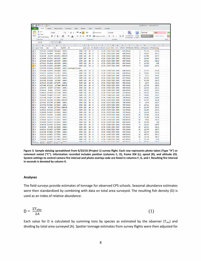
Figure 3. Sample datalog spreadsheet from 6/23/16 (Project 1) survey flight. Each row represents photo taken (Type “X”) or comment noted (“C”). Information recorded includes position (columns C, D), frame ID# (L), speed (R), and altitude (O). System settings to control camera fire interval and photo overlap code are listed in columns F, G, and I. Resulting fire interval in seconds is denoted by column K.

Analyses

The field surveys provide estimates of tonnage for observed CPS schools. Seasonal abundance estimates were then standardized by combining with data on total area surveyed. The resulting fish density (D) is used as an index of relative abundance.

D = ΣTobs ΣA

(1)

Each value for D is calculated by summing tons by species as estimated by the observer (Tobs) and dividing by total area surveyed (A). Spotter tonnage estimates from survey flights were then adjusted for

9

observer bias based on SCB point set data collected in 2010 by our current spotter as part of the NWSS effort (Jagielo et al. 2010, see below - Uncertainty for Biomass Estimates derived from 2010 Point Sets).

Actual area surveyed (A) is determined by GIS analyses of the survey transect flight paths multiplied by transect width (Appendix 2). A transect width of 1200 meters was determined in mid-2015 by examining plots of observed tonnage at a given distance from the plane for each altitude (Appendix 1). Plotting number of detections versus distance from transect line revealed 1200 meters as a reasonable average distance at which observer sightability was consistent for previous seasons flown at both 1000 and 1500 feet.

The area able to be searched varies, depending on conditions; the outer limit can be affected by glare from the sun or sea conditions. If the water is glassy, visibility is extended further, and the observer can see “breezers” further away (disturbances on surface indicative of fish schools); if it is windy, the whitecaps will obscure the view. Our observer noted that there is a blind spot of approximately 20 degrees angled from a line straight down from the plane to a distance off the transect line (equivalent to 166 meters @ 1500 feet altitude and 111 meters at 1000 feet). Since blind spot areas under the plane fuselage were not actively searched while on transect, they were subtracted from the 1200 m detection distance area.

In the case of schools straddling survey area boundaries (inside and outside of transect width), we included the estimated tons but not the additional area in our index calculations. We define Tobs as total tons observed and A as area effort (only the area surveyed).

Second replicate surveys were conducted for some seasons based on weather conditions and availability of resources. All replicates were treated as separate indices of abundance. Some replicates were not complete surveys, as specific areas may not have been surveyed due to persistent inclement weather conditions.

Index values (D) are calculated for each survey flown during a season. For each index, nearshore island observations are combined with mainland observations to obtain total nearshore estimates of abundance.

Uncertainty for Biomass Estimates derived from 2010 Point Sets

The West Coast Aerial Sardine Survey in 2010 included efforts to collect data in Southern California. Included in the protocol was at-sea point set sampling used to determine the relationship between individual school surface area and the biomass of individual fish schools (Jagielo et al. 2010). This sampling involved spotter aircraft working closely with fishing vessels to locate and completely wrap sardine schools. The lead spotter involved in identifying and quantifying sardine schools was the same individual as the sole observer for the SCCPSS.

This data set included spotter estimates from the air as well as landed tonnage, allowing for validation of tonnage estimate accuracy. School sizes (2.9 – 84.9 landed metric tons) encompassed the range of

10

individual-sized schools seen on SCCPSS surveys. SCCPSS raw tonnage estimates were adjusted with a correction factor (r = Σ Tons landed / Σ Tons observed) derived from the 2010 data.

Data from 29 of the point sets from the 2010 survey were used to determine observer accuracy and variance (Table 2). These point sets were chosen because data were available (observer-estimated tons, observer-estimated % wrap of the school, and actual landed tons) that would allow comparison of observer-estimated tons with landed tons. The observer estimates were adjusted for % wrap of the schools by multiplying observer-estimated tons by the % wrap of schools to get adjusted estimated tons (x), and then compared to landed tons (y).

Table 2. 2010 point set data (n=29) used to determine biomass estimate correction factor and variance for observer-estimated tonnage.

Landed Tonsi x y y/x rj-r0 wj [wj(rj-r0)]21 5 4.8 0.97 -0.133 0.00568 0.00000062 27 40.2 1.49 0.385 0.03069 0.00013963 22.5 25.7 1.14 0.041 0.02558 0.00000114 30 38.5 1.28 0.181 0.0341 0.00003825 5 10.1 2.02 0.919 0.00568 0.00002736 15 10.9 0.73 -0.377 0.01705 0.00004147 15 15.4 1.02 -0.079 0.01705 0.00000188 9.5 15.0 1.57 0.472 0.0108 0.00002599 5 6.7 1.35 0.242 0.00568 0.000001910 10.8 17.9 1.66 0.556 0.01228 0.000046611 10 2.8 0.28 -0.819 0.01137 0.000086712 10 9.6 0.96 -0.142 0.01137 0.000002613 9.5 14.9 1.56 0.460 0.0108 0.000024714 25 20.0 0.80 -0.302 0.02842 0.000073715 11.4 10.7 0.94 -0.161 0.01296 0.000004416 47.5 58.7 1.24 0.133 0.054 0.000051317 25 31.3 1.25 0.150 0.02842 0.000018118 35 44.0 1.26 0.153 0.03979 0.000036819 61.75 67.4 1.09 -0.012 0.07019 0.000000720 45 45.0 1.00 -0.103 0.05115 0.000027521 49.5 38.8 0.78 -0.319 0.05627 0.000322022 52.25 23.9 0.46 -0.645 0.0594 0.001467323 42.75 46.8 1.10 -0.008 0.0486 0.000000224 80 84.9 1.06 -0.042 0.09094 0.000014625 23.75 20.2 0.85 -0.253 0.027 0.000046826 50 64.2 1.28 0.181 0.05684 0.000105327 31.5 40.5 1.29 0.182 0.03581 0.000042328 50 76.8 1.54 0.433 0.05684 0.000604929 75 84.6 1.13 0.025 0.08526 0.0000044

Sum 879.70 970.55 1 0.0032586

r0 = Σy/Σx = 1.1033 0.003374998SE = 0.058094732

Adjusted Plane-Estimated Tons

V(r0 ) = [wj(rj-r0)]2 [n/n-1] =

11

From these data, we determined:

1) A correction r0, where

r0 = Σtons landed/Σtons estimated = Σy/Σx= Σ (wj∙rj) = 1.103.

The term r0 was applied to the survey observer tonnage estimates (C) to get adjusted biomass estimates.

2) Variance C2*V(r0), where

C = observer-estimated tons,

V(r0) = Σ (wj∙ (rj-r0)2) ∙ (n/n-1) = 0.00337, where

wj = weight (each estimate of adjusted tons/total adjusted estimated tons),

rj = each jth value of y/x.

This variance formula (see Cochran 1977) used weighted values of y/x and was applied to each adjusted biomass estimate from 1) above to determine variances of the biomass estimates. The tonnages and variances of individual observations were then summed to obtain total tonnage and relative error for each season’s survey(s).

Boat Sampling

Boat sampling was conducted to validate observer identification of species, and provide information on size and age structure of the observed fish. To date, boat sampling has been conducted for Project 1 work only. Separate flights from the transect flights were paired with boat-based sampling of CPS schools observed from the air. Boat surveys were guided to specific areas for sampling by aircraft observations of CPS. Waters off Santa Catalina Island and off the northern Orange County coast have been sampled (Figure 4). Underwater video and hook-and-line sampling methods were used to validate aerial observer identification of species, and collect samples to provide information on size, maturity and age of the observed fish. The 2012 sampling used a Deep Blue Pro Color tow camera and hook-and-line gear. Due to challenges from the tow camera disrupting fish behaviors and poor image quality, beginning in 2013 video sampling was conducted by divers. Hook-and-line samples were collected using sabiki rigs.

12

Figure 4. Locations of successful boat sampling efforts, 2012 – 2015.

In 2015, net sampling methods were first employed in an effort to increase sampling efficiency. The hook-and-line gear remained as an alternate method. A 50-foot length monofilament gill net with a mixed mesh of 1 ¼ to 2 ½-inches that was manually deployed and retrieved. This method was ineffective on moving schools of fish, and our sample size remained lower than with hook-and-line. In 2016, we attempted to manually deploy and retrieve a 200-foot variable mesh purse seine net off. This method proved ineffective as deployment was slow and cumbersome allowing the fish to avoid the net. No samples were collected with the purse seine net. With all methods, sampled fish were bagged, tagged according to school, and preserved on ice for lab work. Once in the lab, samples were processed and weight, length, sex, maturity and age data were recorded using methods consistent with CDFW CPS wetfish port sampling and ageing protocols (CDFW 2014, Yaremko 1996). Aerial species identifications were noted and compared with results of boat sampling (Table 3).

13

Table 3. Boat sampling results. Aerial identifications from observer (blue shading) were compared to boat sampling results. Matches defined as consistent with aerial observations, but may not include all species identified from the observer.

Species: PS = Pacific Sardine; PM = Pacific Mackerel; JM = Jack Mackerel; NA = Northern Anchovy

A Secchi disk was used to determine water clarity, and a Bio Marine model ABMTC refractometer was used to measure water specific gravity and salinity. Data on SST, school density depth, and water depth were collected from a Furuno® Nav-net display and DFF1 digital network echosounder (2,500-foot range with dual-frequency 50/200 kHz), and data on temperature and light intensity at depth obtained using an Onset HOBO Pendant Temperature/Light Data Logger.

Project 2: Develop an inshore correction factor to account for sardine and anchovy not sampled in offshore acoustic surveys

Since 2006, ATM surveys have provided information on CPS abundance off the Pacific coast of North America. Due to operational restrictions, these surveys have operated in waters deeper than approximately 40 meters in depth. This has led to concerns over CPS abundance missed in waters inshore of ATM transect lines. The May 2016 PFMC workshop recommendation led to SCCPSS initiating a

Aerial IDDive Tow Video Hook and Line Net* PS PM JM NA

PM, PS UNID PM, JM 5 PM, PS PM, JM PM, PS 1 2

PM, PS (mostly PM) UNID PM, JM 5 1 PM, PS PM?, PS? PM, JM, Blacksmith 9 1

PS, PM? (mostly PS) PM, PS PM PS, NA No video - turbid lizardfish, croaker, smelt

Mackerel (mixed?) PM, PS PS, PM PM, JM, Blacksmith PM, PS PS? PM, PS, JM PM, PS PM, PS PS? PM, PS, JM 2 4 1

PM, PS (mostly PM) PM, JM, PS PM, possibly JM PM, JM 2 2 Mostly PM PM, JM PM, possibly JM PM, JM 20 3

PS, PM PS, PM 2 4 NA NA 2

NA or PM PM, JM, smelt 3 2 PM, NA PM, JM, NA 2 2 1

NA NA 36 NA PM, JM 10 7NA PM 7

Summer 2014 PM, PS (mostly PM) PM 14 JM, PS PM 3

PS, PM PM, JM 7 1 PM PM 14

PS, NA, M

PS, MMix

Boat ID # Samples Taken Match

Summer 2012

Spring 2013

Summer 2013

Spring 2014

Summer 2015 *gill net

Summer 2016 *purse seine net

Season

14

pilot study in September 2016 to attempt to fly directly over ATM transects and continue to shore, with the goal of deriving inshore correction factors (PFMC 2016b).

Field Methods

The methods described above for Project 1 regarding fish sighting, identification, documentation, and tonnage estimate adjustment also apply to Project 2. In September 2016, the SCCPSS flew overflights of 5 acoustic trawl transect lines in the SCB (Figure 5). The survey aircraft conducted overflights of existing ship transects within the SCB to collect data to compare sightings between aircraft and ship while the ship ran its SCB survey. The study area was based on the 17 transect lines currently used by the ATM survey in the SCB (J. Zwolinski, pers. comm., Figure 5). SCCPSS staff coordinated with the ATM survey to conduct survey flights over the innermost 20-nautical mile segment of the ship transects on the same day as the ship surveys. The aircraft then continued from the most inshore point of the transect line all the way to shore to survey fish schools not surveyed by the ATM. Efforts were made to fly as many of these transects as possible while the ship surveyed the SCB. The 2016 flights flew three replicates for each line, but this will be reduced to a single replicate for future surveys to avoid potential double counting. Observed fish species and tonnages from the areas covered by both aircraft and ship can be compared to evaluate what was detected by each survey method. A correction factor (see Analyses below) can be developed from these data to account for fish in the nearshore area not sampled by the ATM survey. These results can be used to adjust ATM survey estimates to account for biomass inshore of the transect lines.

Figure 5. Project 2 ATM transect lines and overflight observations, September 2016.

15

Analyses

For Project 2, the goal is to provide an inshore correction factor for estimating total CPS abundance within the SCB. This can be done through development of an adjustment for the negative bias of ATM survey biomass estimate to account for fish shoreward of ATM transects. The correction is determined using proportionality of fish observed by the aircraft in both inshore and offshore areas; this ratio is applied to offshore estimates from the ATM survey in the SCB to obtain biomass estimates that account for nearshore fish. Figure 6 is a schematic of the areas around an ATM transect line pertinent to the calculation of the inshore correction factor.

Figure 6. Diagram of areas included in inshore correction factor calculation (see text for formula and explanation). Representative ATM transect line extends from label (“Transect line”), bounded by red vertical lines.

T = TA + (Σ TC / Σ TBp) * TBs (2)

T = total absolute biomass estimate within SCB (metric tons)

TA = metric tonnage represented by area A (A = total SCB area within ATM transect lines)

TC = metric tonnage represented by area C (C = area the aircraft surveyed on the transect line from the inshore end to beach

TBp = metric tonnage represented by area Bp (Bp = area of overlap on transect line where ship and aircraft both surveyed)

TBs = metric tonnage represented by area Bs for the expanded estimate of biomass for the area covered by the ATM survey (Bs = total area within ship-aircraft overlap for which ATM biomass estimates are produced in the SCB)

Alternatively, the SCCPSS data from Project 1 can be used as a minimum absolute abundance estimate for SCB nearshore waters, and added to ATM biomass estimates to obtain a total SCB minimum absolute estimate for the SCB.

16

RESULTS

Project 1

Sardine density indices of abundance for both summer and spring surveys have shown increases in recent years (Table 4, Figure 7). Summer indices were at the highest levels in 2012-2013, but sharply decreased for 2014-2015, and increased in 2016. Spring survey densities were low in 2013-2014, but the two most recent years have been the highest yet. The highest frequency and largest aggregations of sardine have been observed along the mainland coast with a smaller number of sightings off the islands (Figure 8). Large concentrations were observed off the Santa Barbara-Ventura, Pacific Palisades, and Orange County coastlines.

Table 4. Sardine and anchovy density indices by season. Note: anchovy included in survey beginning with the Summer 2013 season, and no survey was conducted in Spring 2015. Replicate surveys numbered.

Year Season DatesB (mt) D (mt/km2) RE (%) B (mt) D (mt/km2) RE (%)

2012 Summer 7/30 - 8/17 880 7225 8.21 2.8 - - -2013 Spring 4/22 - 5/21 831 1543 1.86 3.3 - - -

Summer 8/1 - 10/4 945 6278 6.64 3.3 15199 16.08 5.22014 Spring 5/13 - 6/20 2074 3859 1.86 4.2 7612 3.67 10.8

Summer 1 8/4 - 8/18 832 62 0.07 3.2 386 0.88 5.3Summer 2 8/25 - 8/26 370 0 0 - 568 1.54 5.1

2015 SpringSummer 1 8/7 - 8/29 1736 116 0.07 1.8 0 0 -Summer 2 10/1 - 10/6 1650 375 0.23 2.6 0 0 -

2016 Spring 1 4/16 - 5/2 1290 3364 2.61 1.5 1052 0.82 2.0Spring 2 5/23 - 6/23 798 7050 8.83 2.0 4224 5.29 3.9Summer 8/11 - 9/6 1679 7560 4.50 4.8 29 0.02 4.8

(km2)

NO SURVEY

Area Surveyed Sardine Anchovy

17

Figure 7. Density (D) indices of relative abundance by species and mean date of survey dates within summer and dpring seasons (see Table 3 for D values).

0.00

2.00

4.00

6.00

8.00

10.00

12.00

14.00

16.00

18.00

Jan-12 Jan-13 Jan-14 Jan-15 Jan-16 Jan-17

Sardine - Sum Sardine - SprAnchovy - Sum Anchovy - Spr

Den

sity

(mt/

km2 )

Mean Survey Date

18

Figure 8. Sardine observations for seasons Summer 2012 – Summer 2016. Note these are field estimates of tons.

Anchovy densities have generally decreased in both Spring and Summer from the start of the SCCPSS, with one notable exception being the second survey from Spring 2016 (Table 4, Figure 7). Anchovy were observed during the first three field seasons after being formally documented in the survey beginning with Summer 2013. For seasons Summer 2013 through Summer 2014, large numbers were seen off the Santa Barbara – Ventura coast (Figure 9). None were sighted in 2015, with no survey in Spring and none observed in the Summer. Both Spring 2016 surveys saw the highest abundance seen since Spring 2014 (again with large numbers seen off Santa Barbara-Ventura), and observed abundance declined again in Summer 2016.

19

Figure 9. Anchovy observations for seasons Summer 2013 – Summer 2016. Note these are field estimates of tons.

Boat Sampling

Samples were collected off the northern Orange County coastline and Santa Catalina Island (Figure 4). During the time periods of our study, more single-species and mixed schools of Pacific mackerel and northern anchovy were observed relative to sardine. Each season’s boat sampling results indicated accurate aerial identification of CPS. No samples were collected in 2016 due to logistical challenges with weather and boat/personnel availability, and unsuccessful testing of new gears.

Results from the boat sampling were generally consistent with CPS schools identified from the aircraft (Table 3). In some cases, positive identification of species was difficult due to poor video quality, or possibly insufficient sampling by hook-and-line and net methods.

20

Collected CPS samples for 2012-2015 seasons were heavily weighted towards mackerel species, especially Pacific mackerel (Table 5). This may be primarily due to use of sabiki rigs (hook and line) for capture, as Pacific mackerel may have outcompeted other CPS for hooks. The few (n=3) sardine samples collected in 2012 and 2013 were mature females, and anchovy samples from 2014 (n=39) were males and females of intermediate maturity. In the future tow nets or midwater nets may be deployed in attempts to improve the sample size.

Table 5. Biological data from collected boat samples, 2012-2015.

Project 2

Three Project 2 overflights were flown in conjunction with the ATM survey on 9/7/16, 9/14/16 and 9/15/2016 (Table 6, Figure 5).

Avg (g) SD Avg (mm) SD M F U Avg SD Avg SDPS 1 108 - 198 - 0 1 0 3 0 4 0

PM 21 61 29.3 176 18.5 1 0 20 1 0 0 0.3

JM 2 62 7.5 184 6.4 0 2 0 1 0 - -NA - - - - - - - - - - - -

PS 2 127 3.2 208 4.2 1 1 0 2 0 2.5 0.7

PM 4 270 101 266 50.9 2 2 0 2 0.8 1 0.8

JM 1 60 - 173 - 0 0 1 1 0 - -NA - - - - - - - - - - - -

PS - - - - - - - - - - - -

PM 22 131 67.3 222 26.6 2 6 14 1 0 0 0.3

JM 5 83 29.3 251 112.8 2 1 2 1.5 0.5 - -NA - - - - - - - - - - - -

PS 2 126 20.4 198 11.3 0 2 0 3.5 0.7 3 1.4

PM 26 121 20 219 10.5 6 18 2 1.9 0.05 0 0

JM 11 97 25.8 202 14.9 0 4 7 1.3 0.07 - -NA 39 14 4.2 103 11.3 23 15 1 2 0.3 1.4 1

PS - - - - - - - - - - - -

PM 14 207 44.7 255 18.8 5 9 0 1.6 0.5 1 0.4

JM - - - - - - - - - - - -NA - - - - - - - - - - - -

PS - - - - - - - - - - - -

PM 24 117 42.3 216 22.1 7 10 7 2 0.9 0 0.5

JM 1 88 - 195 - 0 0 1 1 0 - -NA - - - - - - - - - - - -

Length Maturity Stage Age in Years

Summer 2013

Spring 2014

Summer 2014

Summer 2015

Summer 2012

Spring 2013

Species # of Fish (n)

Sex CountWeight

Maturity Stages - anatomical classification system based on 3 stages for males and 4 stages for females: 1 = Clearly immature; 2 = Intermediate; 3 = Milt (M) or yolked oocytes (F) present; 4 = Hydrated oocytes present.

Species: PS = Pacific Sardine; PM = Pacific Mackerel; JM = Jack Mackerel; NA = Northern Anchovy

Sex: M = Male; F = Female; U = Unknown

21

Table 6. Project 2 results from September 2016 flights. ATM transect lines 112 and 113 were also flown but no fish were observed. Offshore refers to areas on ATM transect line, inshore refers to areas shoreward of the shoreward endpoint of ATM line. Observations on 9/14/16 (shaded yellow) were from an opportunistic survey extending transect line 111 due to sighting of R/V Reuben Lasker. The only inshore survey observations were sardine, and the only offshore observations were anchovy.

On 9/7/16 the survey flew over transect 103; low clouds caused a delay in the plane’s departure and necessitated flying below 1000 feet to see the water. One school of anchovy was seen on line 103.

For 9/14/16, the aircraft flew lines 111 and 112. Three schools of sardine ranging from 0.2 to 7 tons were seen about 20 nm offshore on the transect. The R/V was spotted as the last replicate was flown and an additional survey area starting at the vessel and about 5 nm in length was flown.

The flight on 9/15/16 covered lines 113 and 114. Anchovy were spotted on the overlap on line 114 and sardine near the coast. Similar to the flight on 9/14, conditions were favorable to begin the day, but winds picked up to 10 knots later on, making conditions less than ideal for the second lines flown those days (lines 112 and 114, respectively).

The proposed inshore correction factor equation can only generate a biomass estimate that accounts for nearshore fish if schools are observed in both inshore (TC) and offshore (TBp) areas. In Summer 2016 there were no transects where schools of the same species were observed both inshore and offshore. Therefore, a correction factor could not be calculated. The sardine observations made on 9/14/16 were part of an opportunistic survey that occurred greater than 20 nm offshore as a result of the R/V Reuben Lasker being spotted.

Sardine Anchovy Latitude Longitude9/7/2016 103 6 X 34.2798 -119.5077

9/14/2016 111 3 X 33.315 -118.24089/14/2016 111 7.2 X 33.3318 -118.2369/15/2016 114 4 X 33.1452 -117.37289/15/2016 114 4 X 33.1581 -117.37949/15/2016 114 4.5 X 33.1485 -117.37259/15/2016 114 11 X 33.0379 -117.58739/15/2016 114 3.5 X 33.133 -117.36189/15/2016 114 3.5 X 33.128 -117.3559/15/2016 114 3 X 33.1419 -117.35239/15/2016 114 2.5 X 33.1358 -117.36329/15/2016 114 0.5 X 33.0486 -117.5793

Biomass (mt) LocationDate Line Offshore Inshore

22

DISCUSSION

Proposed use of aerial survey data in CPS stock assessments

Project 1 data can be used to produce an index of abundance in biomass/unit area of transect within approximately two nautical miles of shore in the SCB that may be used as a measure of relative abundance in an integrated stock assessment. In addition, if the estimate from the aerial survey is treated as a census estimate of absolute abundance shoreward of the ATM survey transect lines and timed to coincide with the ATM survey, the estimate could be added to the estimate of abundance from the ATM survey to provide a complementary absolute estimate of abundance in the SCB. The latitudinal distribution of the current SCCPSS sampling program does not include portions of the range of CPS outside the SCB, which could be added in the future to provide more comprehensive coverage of each species range.

Project 2 may provide a means of expanding the offshore biomass estimated from the ATM survey to account for the biomass shoreward of the ATM survey lines within the SCB. The survey data may be used to calculate a ratio of onshore to offshore abundance along latitudinal transects. If data were collected at a sufficient interval and replication to provide a suitable precision to expand the ATM survey estimates to account for abundance shoreward of the ATM survey, the results would provide a total absolute estimate of abundance for the SCB. Expansion of the sampled range beyond the current pilot project to include transects northward would allow similar adjustments along the entire range of the species in question. Collaboration with the ATM survey to focus sampling on the range of focal species determined by the ecological distribution model in the case of sardine or the full distribution of the central subpopulation of northern anchovy would allow more comprehensive sampling of the entire population in the future.

The biological data from specimens collected by the vessels in the vicinity of schools identified in the course of the Project 1 in nearshore waters can be used to inform sex ratio, length/age composition and maturity of the schools in the vicinity. The timing of sampling of Project 2 to coincide with the ATM survey would allow offshore samples collected by the ATM survey to provide opportunistic, but representative samples of the age composition of the fish identified in the aerial survey. Sampling shoreward of the ATM transects during Project 2 can provide representative sampling along the remainder of the transect line. The biological data collected can be used to complement indices of abundance in an integrated assessment.

Assumptions

There are several assumptions concerning the use of the collected data. One is that the survey method (including detection and range coverage) results in data that accurately and consistently represents the abundance of the sardine and anchovy stocks. The survey is a daytime visual survey that assumes fish within approximately the upper 10 meters of the water column are detected. The fish that inhabit those depths during the day serve as the index for the entire stock; additional studies of depth-dependent abundance in these waters would need to be undertaken to verify this. Thus, the index value may be

23

affected by variation in the detection probability given environmental conditions should they prevent schools from being observed over the course of a transect.

Some of the schools may not be visible given their depth distribution or environmental conditions, thus use of the results from Project 1 as a census of abundance inshore of the ATM survey should be treated as estimates of minimum abundance. For Project 2 that is less the case, as the depths increase and the chances of missing fish at depth may increase if they are distributed in deeper depths than are observable by the spotter. Even though the specific transects and study areas are chosen for each survey day according to weather and ocean conditions, such factors may affect the results of both surveys. Survey flights were conducted only when skies were clear and winds calm; this serves to standardize to a large extent variations in sighting conditions. However, there were still occasions where conditions were not ideal, as the aircraft passed through localized weather patterns, or conditions changed as the survey proceeded.

The Project 2 method and formula to determine inshore abundance assumes that an equal proportion of the biomass that is present offshore and nearshore is visible to the spotter. The proportion of the biomass visible in each area may vary based on depth distribution of the school and visibility. If the proportion visible is greater offshore, the ratio will be biased low. If the proportion visible is greater inshore it will be biased high. If the proportion of the biomass in each area that is visible to the spotter is equal, it should be unbiased, all other things being equal. More field studies are necessary to collect sufficient data to adequately evaluate the effects of differences in detection probability in each area on the results of this method.

Weather was a primary factor behind SCCPSS seasons ultimately surveying different parts of the study area. The density indices calculations included all data for all survey seasons without regard to specific areas actually surveyed for each survey season. The assumption was that the density across all areas, either mainland or island, would be unbiased. An alternative method would standardize these calculations for area type, perhaps by only considering survey data from commonly surveyed areas (i.e., mainland areas). In addition, the chance of double counting the same fish on separate sampling days or surveys is not accounted for in the index calculations.

During the spring, the southern range of the northern subpopulation of sardine includes the SCB, but with summer and warmer waters is shifted northward out of the SCB, while the southern subpopulation also shifts north into the SCB (Felix-Uraga et al. 2004, 2005). Therefore, spring survey estimates are believed to belong to the northern subpopulation, and data from the spring sampling period would be the pertinent dataset on which to base an index for management. Habitat models can provide detailed information on differentiation of subpopulations at specific locations and time periods. For both sardine and anchovy, the complete range of these stocks extends north (for both species) and south (for anchovy) of the study area.

Boat Sampling

Aerial and boat-based species identification of fish were consistent (Table 4). Additional sampling for single-species sardine and anchovy schools would be useful to validate aerial identification accuracy for

24

these species. Along with exploration of other methods to increase sample size, a more varied range of geographical boat sampling, such as off the SCB north coast or the northern Channel Islands, as logistics allow, would provide improved validation of species identification and data on representative length/age composition. Further attempts to collect sardine and anchovy samples across the study area would better describe the demographics of these stocks at the time of the survey, and inform size and age selectivity within assessment models used for management.

Biological information from CPS samples was also limited by the relative inefficiency of collection methods (Tables 5 and 6). Attempts to increase sample size using gill and purse seine nets were difficult and inefficient given the lack of experience with methods and equipment. In our efforts, gill nets were more manageable than the purse seine net, but it is not the preferred method for capturing CPS in the SCB. A small midwater trawl net is being considered for the next season that could be more effective in collecting samples. There is a trade-off required, where the boat needs to be fast and maneuverable enough to set on schools located by the aircraft, as well as being capable of safely operating in ocean waters and hauling gear. Video and hook-and-line gear remain the simplest alternative methods to help validate species identification while different net options continue to be explored to provide biological samples for length and age composition data.

25

Responses to April 17-18, 2017 Review Panel Requests

The following are from the review panel report, with additional CDFW comments in bold.

A. Request: Update Tables 1 and 2 from the report of the June 2009 Methodology Panel on the Northwest Aerial Survey (PFMC: Agenda Item H.2.A. Attachment 3, June 2009). Rationale: The Panel wished to have a single summary of the key sources of uncertainty, how the estimates of biomass were likely to be impacted by each source, and whether it would be possible to address each uncertainty, and estimate its magnitude. Response: Table 1 lists the sources of uncertainty associated with species identification, school detection and biomass estimation. It also lists the likely direction of bias and data / methods to overcome each source of uncertainty. The primary sources of uncertainty/bias in Table 1 not currently addressed by the survey are schools too deep and surveyor bias (with regard to both species misidentification and biomass estimation). One way to address schools deeper than visual detection limits is to compare total nearshore biomass from acoustic studies with observed biomass from aerial observations. Currently the survey uses one surveyor. CDFW will be considering using alternate surveyors and appropriate calibration studies to account for multiple surveyor observations.

B. Request: Show the variance estimates and how they are calculated. Ideally, quantified uncertainty would account for within-transect error (replicate sampling) that might indicate depth variation and movement in schools plus surveyor error. Between-transect variance and the variance estimator for the biomass estimate were requested. There also appears to be rounding since there appears to be an improbable set of numbers divisible by five given the numbers presented. Would that contribute to the variance? Is there an estimate of surveyor bias or survey condition bias? A table listing the sources of variance, how they are calculated, and how they are combined to estimate biomass estimation error would be helpful. Rationale: The estimates of variance of total Coastal Pelagic Species (CPS) biomass included in the documentation accounted only for survey bias error derived from the point set data. Response: The Panel and proponents agreed that the current approach to quantifying uncertainty is inadequate. Appendix 2 outlines a generic approach for quantifying uncertainty for Project 1 estimates. Variance estimation is discussed further in Section 6.2. See Appendices 2 and 3, and Table 5 of panel report. CDFW aerial survey staff will work with internal statistical staff to develop a variance estimator that is appropriate to the survey. C. Request: Define the standard for “synoptic” needed to reduce the risk of double counting schools from the ATM survey or vice versa. Optimally, it would be good to see comparisons (aerial to aerial and aerial to acoustic) for overlapping data with increasing time gaps between results. If the comparisons between methods worsen over time, that information might be useful for estimating method error. Rationale: The effect of fish movement, whether lateral or vertical, has not been accounted for in the survey analysis. Schools of sardine or anchovy can travel 10 nm during 24 hours, which can bias estimates from combined aerial-acoustic survey data. The probability of counting the same schools twice may increase with the time interval between the aerial and ATM surveys.

26

Response: The proponents highlighted that aerial surveys are generally conducted very quickly (1-2 days), and attempts are made to conduct aerial surveys synoptically with the ATM survey. The Panel supports the strategy adopted by the proponents.

The degree to which the timing between sampling segments of the coast covered in the aerial survey and the acoustic trawl survey transect coverage are sufficiently synoptic to mitigate the potential for double counting depends on the rate of lateral movement of schools between sampled areas. Mobility of the species, strength of currents and potential for overlap in sampling efforts between sampled areas will all contribute to the potential for schools to move between sampling areas and be observed twice. Some degree of double counting would result in error that falls within the variance generated by other aspects of sampling error from observation error (unobserved fish deeper than are visible or shallower than are detectable in the ATM survey) and measurement error (backscatter or spotter estimates/rounding vs actual abundance). Given sufficient time, large schools could move from one sampling frame to another and enough of them counted twice across areas to result in a significant overestimate of biomass.

Fish residing in nearshore areas are generally thought to be subject to less movement due to currents as a result of the friction presented by bottom structure (referred to as “sticky water” by Wolanski (1994)). These areas also offer the opportunity for fish to use vertical migrations to maintain their position. Smaller fish may be less capable of making directed movements than larger fish and northern anchovy are not as strong of swimmers as Pacific sardine, which can move more rapidly (Blaxter and Hunter 1982). As a result, the time frame over which movement between sampling areas becomes a factor depends on a combination of considerations. The time frame over which stationarity in the pattern of distribution can degrade depends on a combination of circumstances, making it unpredictable.

Examination of repeated sampling over the same transect can provide some indication of the time over which stationarity in the pattern of observed distribution degrades. This may not relate directly to the potential for double counting, but rather differences in depth distribution resulting in the school residing in depths greater than are observable by the spotter as well as lateral movement to outside the transect area. Optimally, it would be good to see comparisons (aerial to aerial and aerial to acoustic) for overlapping data with increasing time gaps between results. If the comparisons between methods worsen over time, that information might be useful in estimating method error. Unfortunately, only limited data from replicates conducted offshore with a lag of only a few minutes are available, which is an insufficient duration to provide a meaningful analysis. Additional research examining lags of minutes, hours and one or more days between replicates would be more informative.

In the absence of definitive time frames over which the potential for double counting increases, timing between sampling of separate areas during the course of the aerial survey or ATM survey should be minimized to mitigate the possibility. The forecasts for the next few days can be reviewed to ensure that sampling of the entire survey area can be completed before beginning sampling. In addition, if the direction of movement of the species is known, sampling against the direction of

27

movement will minimize the potential for double counting. Such consideration should be borne in mind when coordinating and conducting sampling.

D. Request: Explain the relationship between the estimates obtained during the Spring and Summer surveys and which subpopulations of anchovy and sardine are observed during those surveys. Rationale: The Panel was concerned that the Summer estimates of biomass likely pertain to the Southern Subpopulation of Pacific sardine. Response: Table 2 suggests that most of the Summer surveys were not conducted in environmental conditions consistent with the presence of the Northern Subpopulation of Pacific sardine. The Southern California Bight is an area of overlap for the two subpopulations, and the Summer data would not provide usable information on the northern subpopulation. Sampling could, however, be shifted northward according to the distribution of the northern subpopulation from the model of Demer and Zwolinski to focus minimum abundance estimates away from the region of sympatry in the summer months. Northern anchovy may occur in the Southern California Bight in summer, thus surveying in the Bight is still worthwhile to provide an estimate of minimum abundance therein, but estimation of Pacific sardine could not be used for management purposes until the latitude of distribution of the northern population is reached. [CDFW comment included in Response] E. Request: Plot (a) the point set data and (b) the ratio data vs. pilot-estimated tons (Table 2 of the survey report). Assess the variance structure of the ratio data to determine whether it matches the assumptions of the analyses or whether another analysis provides a better match. Update the analysis based on most appropriate approach for representing variance. Rationale: The estimate of “r” (and its variance) depends on how the ratio data are weighted. Response: An initial regression suggested that variance is independent of the pilot estimate of biomass. However, it was noticed that the observer biomass estimates rather than the boat-based biomass estimates were corrected, i.e. the observer estimates of school biomass were reduced to better match the actual portion of the school captured, but the relationship which should be explored is that of the observer estimates to the true size of the school, as measured by capture, so the capture amounts should be scaled up instead. See Request K. See plots included in panel report and comment for Request K.

F. Request: Consider and analyze potential stratifications (e.g., coastal vs. island) to reduce bias in the index/estimate when areas are missed during the survey. Rationale: The Panel was interested in knowing whether densities differed spatially. Response: Results indicate that the nearshore (<40m depth) densities around the islands are substantially smaller than those by the coast. No anchovy were seen in any of the surveys around the islands. This indicates that conducting the aerial survey around the islands is unlikely to yield useful results in Summer. In Spring, when the Northern Subpopulation of Pacific sardine is present, the island areas could be surveyed and treated as a separate stratum from the coastal areas. CDFW is considering the relative benefits of surveying island areas, given the relative lack of observations and data. Resources may be better used towards replicates of mainland areas.

28

G. Request: Describe how a recruitment index would be developed given (the lack of) compositional data? Rationale: There is very little age-composition data for Pacific sardines and northern anchovy. However, young-of-year anchovy, as opposed to sardine, do aggregate in the nearshore or other areas, and a coast-wide nearshore aerial survey with directed net sampling may be able to provide an index. Response: The proponents agree that it is currently infeasible to construct an index of recruitment. The nearshore areas are nursery grounds for young of year Pacific sardine and northern anchovy thus the aerial survey was considered as a source of data informing a recruitment index. Complicating direct use of the data from the aerial survey for this purpose is the utilization of the nearshore areas sampled by the survey as foraging grounds for older age classes. Parsing the biomass estimated from the aerial survey to age classes requires biological sampling from the boat-based aspect of the survey to provide length or age composition data. The boat-based survey has not yet developed a sampling method that can efficiently provide an adequate number of samples with which to represent the age composition of fish encountered in the aerial survey. In addition, the selectivity of the gear would need to be determined in order to adjust the sampled catch to better reflect the composition of the sampled school. The sampling frequency and stratification to which the sampled schools could be applied, if only a subset of schools can be sampled, would need to be determined. While use of the aerial survey to provide a recruitment index may be a possibility in the future, the efficiency of sampling methods, frequency of boat based sampling, selectivity and stratification would need to be considered and addressed before a representative index is derived from the survey. The SWFSC YOY rockfish survey provides useful information regarding recruitment and adult abundance using bongo and midwater trawl sampling, sampling closer to shore than the ATM survey. Given the challenges facing the current survey and cost considerations, as well as the availability of this alternative data source, intensified boat based sampling in pursuit of a recruitment index from the aerial survey may be forgone to focus efforts on expansion of the survey area to cover a larger portion of the coast. There is still value in pursuing boat-based biological sampling providing data on the size/age composition of the catch to inform composition of schools encountered during the course of the survey. The sample sizes provided by the ATM survey offshore are lower than may be desirable and may not provide data representative of the composition of fish in the nearshore waters given the greater prevalence of younger year classes. Even without development of a recruitment index, intensified boat based sampling in the nearshore with more efficient sampling methods may be worthwhile for the purpose of biomass projections.

H. Request: Provide more information on species/amounts for split schools to estimate the proportion of schools with mixed species Rationale: The Panel wished to assess the extent to which it is necessary to estimate the precision associated with estimates of species composition by school. Response: Table 3 lists the breakdown of the observations (sampling events that consist of multiple schools) by whether the observation is of a single species or mixed species. It also shows the number of schools within the single-species or mixed-species observations and the corresponding biomass that is from single-species or mixed-species observations. The Panel noted that interpretation of these data is complicated because of the way mixed species schools and biomass are defined. However, there is evidence that mixed species cannot be ignored, when computing measures of precision. Row 3 of the table shows a small number of observations leading to a large number of schools, contributing the

29

dominant tonnage of mixed schools. This could indicate anomalous conditions affecting interpretation of these few observations. The data suggest that observations with large numbers of schools or tonnage may require different consideration of uncertainty associated with biomass estimates. Additional boat sampling would help in acquiring data to be compared with aerial observations to analyze this question. Note that “observations”, as defined by SCCPSS staff, can also mean single schools; they are sighting events.

I. Request: Exactly how are transects flown? Does the pilot always circle and descend to observe schools? Document the criteria used by the surveyor to identify species. Rationale: The Panel wished to better understand the survey protocol. Response: The technical team noted “Distinguishing CPS schools from the aircraft is based on structure, color, shine, and movement of schools. For sardine, they’re black-greenish, with a little twinkle. Schools can be either long and stringy or frequently boomerang-shaped (especially when moving) and also balls; often hard-edged. Anchovy are a generic brown color without much shine, and schools are dull-shaped (rounded) of any shape, often blotchy. Mackerel schools are shinier, and individual fish in the school can be detected (especially with binoculars). The big Pacific or blue mackerels can look silver, the smaller Spanish or jack mackerels brownish-green. The shapes of schools are similar to sardine. Large Pacific mackerel are obvious, but it’s hard to distinguish between jack and smaller Pacific mackerel. Also, mackerels break the surface more often than other species, and schools move much faster.” Yes, the aircraft is directed to suspected schools, and circles to verify species and to make tonnage estimates. These actions are frequently at lower altitude, but not always. See pp. 5-7 of this report, under “Field Methods”. J. Request: Explain where fish are if they are not seen by the surveyor on nearshore transects (to consider bias). For example, are they (a) too dispersed in nearshore waters shallower than 40 m to be detected (b) to deep in nearshore waters to be detected, or (c) deeper than 40m (i.e., not in the nearshore zone, and therefore not in this survey)? Rationale: The Panel wished to better understand the survey protocol because of the apparent relationship between the number of schools in a cluster and the percentage of schools identified as sardine versus anchovy. Species identification should not be density-dependent. As with the overcounting risk resulting from lateral fish movement, vertical fish movement can lead to undercounting bias for aerial estimates. Response: Sampling error can be examined using repeated surveys and by repeating transects. The magnitude of bias due to dispersed schools and fish deeper than 10m could be consequential (negative bias), but there are currently no data to estimate the magnitude of this bias. The Panel did not consider fish deeper than 40m and offshore a major concern because the nearshore is a strip survey. Agreed; if not observed, the fish are either too dispersed or too deep to be detected. Future surveys will attempt at least 3 replicates of survey areas to inform magnitude of sampling error.

K. Request: Re-plot (a) the point set data and (b) the ratio data vs. pilot-estimated tons, but adjusting the boat-based landed tons rather the pilot (observer) based biomass estimates. Rationale: The data used for analysis should be adjusted landed tons to pilot total school biomass estimates, as the goal is to quantify the relationship between the surveyor-based estimates of entire school biomass and the estimates estimated using point sets, accounting for proportion captured.

30

Response: The analysts adjusted to the data to reflect the recommendation of the panel. The panel noted that 3 of the point sets were estimated to have caught only half of the observed school, while all others were estimated to have caught at least 90% of the school. Since these two points represented extreme outliers either in the ratio or both in estimated biomass and size of the residual, the panel ultimately recommended removing them from the data set, leaving 26 data points. Figures 1 and 2, which plot the remaining 26 data points, confirm the need to conduct a regression through the origin and also that assuming constant coefficient of variation (CV) is not supported by the data. Constant variance or a relationship between observer estimated biomass and variance that is intermediate between constant variance and constant CV should be used when estimating the total variance of the resultant biomass index or estimate. Appendix 3 [of panel report] outlines one method for estimating the variance of biomass from the surveys. The proponents will consider the approach outlined by the panel and will develop a revised variance estimator to be applied to survey data.

L. Request: Estimate the extent of between-island variance in density Rationale: The amount of between-islands variance in density is needed to estimate the variance of density for unsampled areas. Response: There was insufficient information from previous surveys to evaluate consistency in densities among the island areas. See comment for Request F.

M. Request: Provide synoptic, transect-specific acoustic data to compare with the aerial data. Rationale: There is considerable variation among transects and the overall variance of any correction factor depends on the variance of the ATM-based estimates of biomass. Response: Dr. Juan Zwolinski (SWFSC) provided acoustic data for transects that overlap with the aerial survey. However, direct comparisons are difficult to make because the aerial observations occur in the upper 10 m while this represents a “dead zone” with no observations for the acoustic survey. Plots of ATM density and aerial survey biomass for the transects surveyed during 2016 also confirmed that the variation is very high. Agreed, the two surveys are not sampling the same vertical areas, and application of this method for estimating nearshore abundance based on the relative survey abundances from common horizontal transects would be problematic. The only case where this would be valid would be if the vertical distributions between aerial and acoustic surveys were the same for both offshore and inshore areas. This assumption is currently unsupported and would require field studies to validate.

31

ACKNOWLEDGMENTS

We are grateful to a number of individuals for their part in this survey. We thank the CWPA and their executive director, Diane Pleschner-Steele, for their collaboration on this project. CWPA provided the services of our observer and loaned the FMC camera system. Collaborative Fisheries Research West generously supported CWPA for the observer and imaging software for two field seasons from 2013-2014. Tom Evans, Gary Shales and Kevin Kintz of CDFW Air Services ably piloted the survey aircraft on all aerial operations, and Devin Reed was vital in identifying and describing fish in the field. Bill Miller was instrumental in the initial design and planning of this survey, and Marci Yaremko provided support and guidance. We also thank the CDFW Office of Spill Prevention and Response for the use of their boat and staff for their contributions to the boat sampling work: Christian Corbo, Mark Crossland, Sean Moe, and Sau Garcia. In addition, Alex Kesaris, Kenin Greer, Paul Ton, Michelle Horeczko, Elizabeth Hellmers, Dan Averbuj, Kimberli Boone, Ben Chubak, Rachael McLellan, Lindsay Hornsby, Kathryn Johnson, Jeannette Miller, Roy Kim, Julianne Taylor and Mia Roberts assisted in the field and lab work for this study. Joe Weinstein and Phil Law furnished valuable comments on statistical and design aspects of this project. Finally, we acknowledge the helpful discussions and comments from the CDFW aerial survey team and staff: Briana Brady, John Budrick, Chelsea Protasio, Anna Holder, and Michelle Horeczko; and NMFS staff: Emmanis Dorval, Kevin Hill, Juan Zwolinski, David Demer, Nancy Lo, Paul Crone, Richard Parrish and Mark Lowry.

32

LITERATURE CITED

Blaxter, J.H.S., and Hunter, J.R. 1982. The biology of the clupeoid fishes. In: Advances in Marine Biology, Vol. 20, ed. J.H.S. Blaxter, F.S. Russell, M. Yonge, pp. 1–223. London: Academic Press.

California Department of Fish and Game (CDFG). 2001. California’s living resources: a status report. 592 p.

California Department of Fish and Wildlife (CDFW). 2014. Laboratory procedures for processing wetfish. 2 p.

California Department of Fish and Wildlife. 2015. California Department of Fish and Wildlife Report on Recent Coastal Pelagic Species Landings. PFMC, November 2015 Briefing Book, Agenda Item H.3.a, Supplemental CDFW Report. 3 p.

Cochran, W. G. 1977. Sampling techniques (3rd ed.). New York: John Wiley & Sons.

Feilx-Uraga, R., V. M. Gomez-Munoz, C. Quinonez-Velazquez, F. N. Melo-Barrera, and W. Garcia-Franco. 2004. On the existence of Pacific sardine groups off the west coast of the Baja California Peninsula and southern California. California Cooperative Oceanic Fisheries Investigations Reports 45:146 –151.

Felix-Uraga, R., C. Quinonez-Velazquez, K. T. Hill, V. M. Gomez-Munoz, F. N. Melo-Barrera, and W. Garcia-Franco. 2005. Pacific sardine (Sardinops sagax) stock discrimination off the west coast of Baja California and southern California using otolith morphometry. California Cooperative Oceanic Fisheries Investigations Reports 46:113–121.

Hill, K. T., E. Dorval, N. C. H. Lo, B. J. Macewicz, C. Show, and R. Felix-Uraga. 2007. Assessment of the Pacific sardine resource in 2007 for U.S. management in 2008. NOAA Tech. Memo. NOAA-TM-NMFS-SWFSC-413. 178 p.

Hill, K. T., P. R. Crone, N. C. H. Lo, E. Dorval, and B. J. Macewicz. 2016. Assessment of the Pacific sardine resource in 2016 for U.S. management in 2016-17. Pacific Fishery Management Council, April 2016 Briefing Book, Agenda Item H.1.a. 171 p.

Jacobson, L.D., N.C. Lo, S.F. Herrick, and T. Bishop. 1995. Spawning biomass of the northern anchovy in 1995 and status of the coastal pelagic species fishery during 1994. NMFS, SWFSC, Admin. Rep. LJ-95-11.

Jagielo, T. H., Hanan, D., Howe, R., and M. Mikesell. 2010. West Coast Aerial Sardine Survey. Sampling Results in 2010. Prepared for Northwest Sardine Survey and the California Wetfish Producers Association. Pacific Fishery Management Council, Portland, OR, October 15, 2010. 51p.

Jagielo, T. H., R. Howe, and M. Mikesell. 2012. Northwest Aerial Sardine Survey. Sampling Results in 2012. Prepared for Northwest Sardine Survey, LLC. Pacific Fishery Management Council, Nov 2012 Briefing Book, Agenda Item G.3.a. 82 p.

33

Lasker, R. (Ed). 1985. An egg production method for estimating spawning biomass of pelagic fish: application to the northern anchovy (Engraulis mordax). NOAA Technical Report, NMFS 36. 99 pp.

Lo, N. C. H., B. J. Macewicz, and D. A. Griffith. 2011. Spawning biomass of Pacific sardine (Sardinops sagax) off U.S. in 2011. PFMC, Nov 2011 Briefing Book, Agenda Item F.2.b, Attachment 2. 38 p.

Lo, N.C.H., L.D. Jacobson, J.L. Squire. 1992. Indices of relative abundance from fish spotter data based on delta-lognormal models. Can. J. fish. Aquat. Sci. 49(12):2515-2526.

MacCall, A.D. 1990. Dynamic Geography of Marine Fish Populations. University of Washington Press, Seattle, Washington. 153 p.

Murphy, G. I. 1966. Population biology of the Pacific sardine (Sardinops caerulea). Proc. Calif. Acad. Sci. Vol. 34 (1): 1-84.

Pacific Fishery Management Council (PFMC). 2016a. Coastal pelagic species fishery management plan: as amended through Amendment 15. Pacific Fishery Management Council, Portland, OR. 49 p. http://www.pcouncil.org/wp-content/uploads/2016/05/CPS_FMP_as_Amended_thru_A15.pdf

Pacific Fishery Management Council (PFMC). 2016b. Report of the NOAA Southwest Fisheries Science Center & Pacific Fishery Management Council Workshop on CPS Assessments. Pacific Fishery Management Council, September 2016 Briefing Book, Agenda Item E.2.a. 38 p.

Smith, P. E. 2005. A history of proposals for subpopulation structure in the Pacific sardine (Sardinops sagax) population off western North america. California Cooperative Oceanic Fisheries Investigations Reports 46:75-82.

Squire, J.L., Jr. 1993. Relative abundance of pelagic resources utilized by the California purse-seine fishery: results of an airborne monitoring program, 1962–90. Fishery Bulletin 93: 348–361.

Taylor, P.R. 2015. Investigating a multi-purpose aerial method for surveying inshore pelagic finfish species in New Zealand. New Zealand Fisheries Assessment Report 2015/36. 92 p.

Williams, K. 1981. Aerial surveys of pelagic fish resources off southeast Australia 1973-1977. CSIRO, Div. Fish.Ocean., Rep. 130.

Wolanski, E., 1994. Physical oceanographic processes of the Great Barrier Reef. CRC Press, Boca Raton, Florida. 194 p.

Yaremko, M. L. 1996. Age determination in Pacific sardine, Sardinops sagax. NOAA Tech. Mem. NOAA-TM-NMFS-SWFSC-223. 33p.

Zwolinski, J., D. A. Demer, B. J. Macewicz, G. R. Cutter, Jr., B. Elliot, S. Mau, D. Murfin, J. S. Renfree, T. S. Sessions, and K. Stierhoff. 2016. Acoustic-trawl estimates of northern-stock Pacific sardine biomass during 2015. Department of Commerce. NOAA Tech. Memo. NMFS-SWFSC-559, 18 p.

34

APPENDICES

Appendix 1 - Detection Distance

Estimation of observer maximum detection distance

The aircraft’s point location is recorded at regular intervals as part of the automated flight data log. ArcMap software was used to plot point locations that represent the aircraft’s flight path using the latitude and longitude fields in the flight data log. The SCCPSS procedure is for the aircraft to fly a circle around a school after the observer has made the initial detection so that photos of the school can be acquired. Therefore, the point at which the flight path deviates off of the transect line to begin a circle of the observed school can be used to estimate the location at which the observer detected the school. The flight path point GIS feature classes for each survey date were visually inspected to determine the point locations at which the aircraft deviated from the transect line. Then the FMC photos were inspected to find the photo that captured an image of the fish school or group of schools closest to the location from which the aircraft’s flight path deviated from the transect. A line feature was created in GIS that connected the point at which the aircraft deviated from the flight path and the closest point at which the school was observed. The ArcGIS “Calculate Geometry” functionality was used to determine the length of this line in meters using the NAD 1983 California Teale Albers projected coordinate system. Line length results were summarized and plotted to determine an estimate of maximum distance at which the observer can detect a school. A value of 1200 meters was chosen as the estimate of the observer’s maximum detection distance for all survey years for both altitudes that were flown for coastal areas (Figures A1, A2). Note that these analyses could only be performed on observations that could be paired with a point where it was obvious where the aircraft’s flight path deviated from the transect.

35

Figure A1. Numbers of fish observations (detections) plotted against distance from transect line for coastal surveys flown at 1500 feet altitude (beginning with Summer 2014 season).

Figure A2. Numbers of fish observations (detections) plotted against distance from transect line for coastal surveys flown at 1000 feet altitude (Summer 2012 – Spring 2014 seasons).

0

5

10

15

20

25

0 500 1000 1500

Coun

t of d

etec

tions

Distance from Transect Line (100-m bins)

Detections x Distance - 1500 feet

0

5

10

15

20

25

0 500 1000 1500 2000

Coun

t of d

etec

tions

Distance from Transect Line (100-m bins)

Detections x Distance - 1000 feet

36

Appendix 2 – Area Surveyed

Determination of survey area used in relative abundance density values

The aircraft’s point location was recorded at regular intervals as part of the automated flight data log. ArcMap software was used to plot point locations that represent the aircraft’s flight path for each survey date using the latitude and longitude fields in the flight data log. The ArcGIS Points to Line tool creates a linear representation of the flight path. Portions of the flight path line that represent travel to and from a survey location as opposed to the actual survey transects were identified. Portions of the flight path line that represent circling of schools to take photos are also identified. Segments of the flight path line that represent survey transects (i.e., with transit and circling removed) were buffered by 1200 meters using the ArcGIS buffer tool to create an initial representation of area surveyed. A buffer distance of 1200 meters was chosen since this is the estimate of observer’s maximum detection distance determined from our detection distance analyses. The buffer was only applied to the right side of the line due to the fact that the observer always observes out of the right side of the aircraft. The flight line was then buffered by 166 meters (Summer 2014 to present) or 111 meters (Summer 2012 to Spring 2014) to account for the observer’s blind spot beneath the aircraft.

The blind spot buffer was then used to clip the blind spot area from the 1200 meter buffer. Next, the ArcGIS Merge tool was used to aggregate all of the flight data lines that made up a survey period into one feature class. There are occasional instances where the buffer of one day’s flight path overlaps another day’s buffer. The ArcGIS Dissolve tool is used to merge areas of overlap so that areas of overlap are not double counted when calculating total area surveyed. Then the flight path area is clipped by a coastline feature so that portions of the polygons that overlay land are removed. Finally, the ArcGIS “Calculate Geometry” functionality is used to determine the survey area in km2.

37

Appendix 3 – FMC Camera System

The following are excerpts from the Forward Motion Compensated camera system operations manual from Aerial Imaging Solutions.

38

39

40

41

42

43