1 

Agenda Item C.5 Attachment 1

Full Version Electronic Only April 2018

ASSESSMENT OF THE PACIFIC SARDINE RESOURCE IN 2018 FOR U.S. MANAGEMENT IN 2018-19

Kevin T. Hill1, Paul R. Crone1, Juan P. Zwolinski1,2

1Fisheries Resources Division Southwest Fisheries Science Center

NOAA National Marine Fisheries Service 8901 La Jolla Shores Drive La Jolla, CA 92037, USA

2Institute of Marine Sciences University of California Santa Cruz Earth and Marine Sciences Building

Santa Cruz, CA 95064, USA (affiliated with SWFSC)

Post-SSC CPS Subcommittee Review Draft

Disclaimer: This information is distributed solely for the purpose of pre-dissemination peer review under applicable information quality guidelines. It has not been formally disseminated by NOAA-National Marine Fisheries Service. It does not represent and should not be construed to represent any agency determination or policy.

 

2  

THIS PAGE IS INTENTIONALLY BLANK

 

3  

TABLE OF CONTENTS ACRONYMS AND DEFINITIONS ............................................................................................. 6 PREFACE ...................................................................................................................................... 7 EXECUTIVE SUMMARY ........................................................................................................... 8 INTRODUCTION ....................................................................................................................... 18

Distribution, Migration, Stock Structure, Management Units ............................................... 18 Life History Features Affecting Management ....................................................................... 19 Ecosystem Considerations ..................................................................................................... 19 Abundance, Recruitment, and Population Dynamics ............................................................ 20 Relevant History of the Fishery and Important Features of the Current Fishery ................... 20 Recent Management Performance ......................................................................................... 21

ASSESSMENT DATA ................................................................................................................ 21

Biological Parameters ............................................................................................................ 21 Stock structure ................................................................................................................. 21 Growth ............................................................................................................................. 21 Maturity ............................................................................................................................ 22 Natural mortality ............................................................................................................. 23 Fishery-dependent Data ......................................................................................................... 23 Overview .......................................................................................................................... 23 Landings ........................................................................................................................... 24 Age compositions ............................................................................................................. 24 Ageing error ..................................................................................................................... 25 Fishery-independent Data ...................................................................................................... 25 Overview .......................................................................................................................... 25 Acoustic-trawl survey ....................................................................................................... 25

ASSESSMENT – ACOUSTIC-TRAWL SURVEY ................................................................... 26

Overview ................................................................................................................................. 26 Merits of AT survey-based assessment ............................................................................. 26 Drawbacks of model-based assessment ............................................................................ 26 Additional assessment considerations .............................................................................. 27 Methods................................................................................................................................... 27 Results ..................................................................................................................................... 29 Areas of Improvement for AT Survey .................................................................................... 29

ASSESSMENT – MODEL .......................................................................................................... 30

History of Modeling Approaches ........................................................................................... 30 Changes between Model ALT (2017-18) and the 2014-16 Assessment Model .................... 30 Overview ........................................................................................................................... 30 Time period and time step ................................................................................................. 31 Surveys .............................................................................................................................. 31

 

4  

Fisheries ............................................................................................................................ 31 Longevity and natural mortality ....................................................................................... 32 Growth .............................................................................................................................. 32 Stock-recruitment relationship .......................................................................................... 32 Selectivity .......................................................................................................................... 32 Catchability ....................................................................................................................... 32 Model Description ................................................................................................................. 33 Assessment program with last revision date .................................................................... 33 Definitions of fleets and areas ......................................................................................... 33 Likelihood components and model parameters ............................................................... 33 Initial population and fishing conditions .......................................................................... 34 Growth ............................................................................................................................. 34 Stock-recruitment relationship .......................................................................................... 34 Selectivity ......................................................................................................................... 35 Catchability ....................................................................................................................... 36 Convergence criteria and status ...................................................................................... 36 Changes to the update model (ALT 2018) ........................................................................36 Results ..................................................................................................................................... 36 Likelihoods and derived quantities of interest ................................................................. 36 Parameter estimates and errors ....................................................................................... 36 Growth estimates .............................................................................................................. 37 Selectivity estimates and fits to fishery and survey age-composition time series ............. 37 Fit to survey index of abundance ..................................................................................... 37 Stock-recruitment relationship ......................................................................................... 37 Population number- and biomass-at-age estimates ......................................................... 37 Spawning stock biomass .................................................................................................. 37 Recruitment ...................................................................................................................... 37 Stock biomass for PFMC management ............................................................................ 38 Fishing and exploitation rates ......................................................................................... 38 Uncertainty Analyses ............................................................................................................. 38 Retrospective analysis ...................................................................................................... 38 Convergence tests ............................................................................................................ 38 Historical analysis ........................................................................................................... 39

HARVEST CONTROL RULES FOR THE 2018-19 MANAGEMENT CYCLE ....................... 39

Harvest Guideline .................................................................................................................. 39 OFL and ABC ......................................................................................................................... 39

REGIONAL MANAGEMENT CONSIDERATIONS ................................................................ 40 RESEARCH AND DATA NEEDS ............................................................................................. 40 ACKNOWLEDGMENTS ........................................................................................................... 41 LITERATURE CITED ................................................................................................................ 42

 

5  

TABLES ...................................................................................................................................... 48 FIGURES ..................................................................................................................................... 65 APPENDICES ............................................................................................................................. 99

Appendix A. SS input files for model ALT. .......................................................................... 99

 

6  

ACRONYMS AND DEFINITIONS

ABC acceptable biological catch ALT alternative stock assessment model AT Acoustic-trawl survey BC British Columbia (Canada) CA California CalCOFI California Cooperative Oceanic Fisheries Investigations CCA Central California fishery CDFW California Department of Fish and Wildlife CDFO Canada Department of Fisheries and Oceans CICIMAR Centro Interdisciplinario de Ciencias Marinas CONAPESCA National Commission of Aquaculture and Fishing (México) CPS Coastal Pelagic Species CPSAS Coastal Pelagic Species Advisory Subpanel CPSMT Coastal Pelagic Species Management Team CY Calendar year DEPM Daily egg production method ENS Ensenada (México) FMP fishery management plan HG harvest guideline INAPESCA National Fisheries Institute (México) Model Year July 1 (year) to June 30 (year+1) mt metric tons mmt million metric tons MEXCAL southern fleet based on ENS, SCA, and CCA fishery data NMFS National Marine Fisheries Service NSP Northern subpopulation of Pacific sardine, as defined by satellite oceanography data NOAA National Oceanic and Atmospheric Administration ODFW Oregon Department of Fish and Wildlife OFL overfishing limit OR Oregon PNW northern fleet based on OR, WA, and BC fishery data PFMC Pacific Fishery Management Council SAFE Stock Assessment and Fishery Evaluation SCA Southern California fishery SCB Southern California Bight (Pt. Conception, CA to northern Baja California) SS Stock Synthesis model SSB spawning stock biomass SSC Scientific and Statistical Committee SST sea surface temperature STAR Stock Assessment Review STAT Stock Assessment Team SWFSC Southwest Fisheries Science Center TEP Total egg production VPA Virtual Population Analysis WA Washington WDFW Washington Department of Fish and Wildlife

 

7  

PREFACE

The Pacific sardine resource is assessed each year in support of the Pacific Fishery Management Council (PFMC) process of stipulating annual harvest specifications for the U.S. fishery. Presently, the assessment/management schedule for Pacific sardine is based on a full assessment conducted every three years, with an update assessment conducted in the interim years. A full stock assessment was conducted in 2017 (Hill et al. 2017; STAR 2017). The following report serves as a stock assessment update for purposes of advising management for the 2018-19 fishing year. The update assessment model (ALT) included final landings from 2016, preliminary landings from 2017, and one new AT-based biomass and age composition from the summer 2017 survey. The following report includes three primary sections: first, a timeline with background information concerning fishery operations and management associated with the Pacific sardine resource (Introduction); second, summaries for various sources of sample data used in the assessments (Data); and third, methods/models used to conduct the assessments (Assessment). The Assessment section includes two parts based on the assessment approach (survey and model). In this context, readers should first consult the section ‘Assessment – Acoustic-trawl Survey, Overview,’ which serves as the basis of the report, i.e., justifications regarding the STAT’s preferred assessment approach. The two assessment approaches were evaluated at the formal stock assessment review (STAR) in February 2017. Readers should refer to STAR (2017) for details regarding merits and drawbacks of the assessments highlighted during the review, and final decisions from the Panel concerning both short- and long-term recommendations for adopting an assessment approach for advising management in the future. That is, while the survey-based assessment was viewed as the better long-term approach by both the STAT and STAR Panel, the Panel identified a notable shortcoming of the survey-based assessment in the short-term, given the need to forecast stock biomass one full year after the last survey observation. Both the STAT and STAR Panel agreed that the preferred survey-based assessment could be effectively implemented by shifting the fishery start date several months to minimize the time lag between the most recent survey and the official start date of the fishery, e.g., moving the start of the fishery from July 1st to January 1st would accomplish this goal. To summarize, model ALT presently represents the recommended assessment approach to adopt for the upcoming fishing year (2018-19), with a survey-based assessment that accommodates a more workable projection period recommended for subsequent fishing years. Finally, field, laboratory, and analytical work conducted in support of the ongoing Pacific sardine assessment is the responsibility of the SWFSC and its staff, including: principal investigators (K. T. Hill, P. R. Crone, J. P. Zwolinski); and collaborators (D.A. Demer, E. Dorval, B. J. Macewicz, D. Griffith, and Y. Gu). Principal investigators are responsible for developing assessments, presenting relevant background information, and addressing the merits/drawbacks of the two assessment approaches in the context of meeting the management goal (current estimate of stock biomass each year), which is needed for implementing an established harvest control rule policy for Pacific sardine. An inclusive list of individuals and institutions that have provided information for carrying out the Pacific sardine assessment is presented in ‘Acknowledgements’.

 

8  

EXECUTIVE SUMMARY The following Pacific sardine assessment update was conducted to inform U.S. fishery management for the cycle that begins July 1, 2018 and ends June 30, 2019. Two assessment approaches were reviewed at the STAR Panel in February 2017: an AT survey-based approach (preferred by the STAT); and a model-based assessment (model ALT). Given forecasting issues highlighted in the review (see STAR 2017 and ‘Unresolved Problems and Major Uncertainties’ below), the Panel ultimately recommended that management advice be based on model ALT for the 2017-18 fishing year. The following update of model ALT represents the final base model from the February 2017 STAR (Hill et al. 2017, STAR 2017) with the addition of updated/new landings (2016-17), one AT-based biomass estimate and age composition from the SWFSC’s summer 2017 survey, along with one additional recruitment deviation for estimation of the 2017 year class. Stock This assessment focuses on the northern subpopulation of Pacific sardine (NSP) that ranges from northern Baja California, México to British Columbia, Canada and extends up to 300 nm offshore. In all assessments before 2014, the default approach has been to assume that all catches landed in ports from Ensenada (ENS) to British Columbia (BC) were from the northern subpopulation. There is now general scientific consensus that catches landed in the Southern California Bight (SCB, i.e., Ensenada and southern California) likely represent a mixture of the southern subpopulation (warm months) and northern subpopulation (cool months) (Felix-Uraga et al. 2004, 2005; Garcia-Morales 2012; Zwolinski et al. 2011; Demer and Zwolinski 2014). Although the ranges of the northern and southern subpopulations can overlap within the SCB, the adult spawning stocks likely move north and south in synchrony each year and do not occupy the same space simultaneously to any significant extent (Garcia-Morales 2012). Satellite oceanography data (Demer and Zwolinski 2014) were used to partition catch data from Ensenada (ENS) and southern California (SCA) ports to exclude both landings and biological compositions attributed to the southern subpopulation. Catches The assessment includes sardine landings (mt) from six major fishing regions: Ensenada (ENS), southern California (SCA), central California (CCA), Oregon (OR), Washington (WA), and British Columbia (BC). Total and NSP landings for each region over the modeled years/seasons follow:

 

9  

Data and Assessment The integrated assessment model was developed using Stock Synthesis (SS version 3.24aa), and includes fishery and survey data collected from mid-2005 through December 2017. The model is based on a July-June biological year (aka ‘model year’), with two semester-based seasons per year (S1=Jul-Dec and S2=Jan-Jun). Catches and biological samples for the fisheries off ENS, SCA, and CCA were pooled into a single MEXCAL fleet (fishery), for which selectivity was modeled separately in each season (S1 and S2). Catches and biological samples from OR, WA, and BC were modeled by season as a single PNW fleet (fishery). A single AT survey index of abundance from ongoing SWFSC surveys (2006-2017) was included in the model. The update assessment model (ALT) included final landings from 2016, preliminary landings from 2017, one new AT-based biomass and age composition from the summer 2017 survey, along with one additional recruitment deviation for estimation of the 2017 year class. Model ALT incorporates the following specifications: NSP catches for the MEXCAL fleet computed using an environmental-based optimal habitat

index; two seasons (semesters, Jul-Dec=S1 and Jan-Jun=S2) for each model year (2005-17); sexes were combined; ages in population=10, with nine age bins (ages 0-8+);

Calendar Yr-Sem

Model Yr-Seas ENS Total ENS NSP SCA Total SCA NSP CCA OR WA BC

2005-2 2005-1 37,999.5 4,396.7 16,615.0 1,581.4 7,824.9 44,316.2 6,605.0 3,231.42006-1 2005-2 17,600.9 11,214.6 18,290.5 17,117.0 2,032.6 101.7 0.0 0.02006-2 2006-1 39,636.0 0.0 18,556.0 5,015.7 15,710.5 35,546.5 4,099.0 1,575.42007-1 2006-2 13,981.4 13,320.0 27,546.0 20,567.0 6,013.3 0.0 0.0 0.02007-2 2007-1 22,865.5 11,928.2 22,047.2 5,531.2 28,768.8 42,052.3 4,662.5 1,522.32008-1 2007-2 23,487.8 15,618.2 25,098.6 24,776.6 2,515.3 0.0 0.0 0.02008-2 2008-1 43,378.3 5,930.0 8,979.6 123.6 24,195.7 22,939.9 6,435.2 10,425.02009-1 2008-2 25,783.2 20,244.4 10,166.8 9,874.2 11,079.9 0.0 0.0 0.02009-2 2009-1 30,128.0 0.0 5,214.1 109.3 13,935.1 21,481.6 8,025.2 15,334.32010-1 2009-2 12,989.1 7,904.2 20,333.5 20,333.5 2,908.8 437.1 510.9 421.72010-2 2010-1 43,831.8 9,171.2 11,261.2 699.2 1,397.1 20,414.9 11,869.6 21,801.32011-1 2010-2 18,513.8 11,588.5 13,192.2 12,958.9 2,720.1 0.1 0.0 0.02011-2 2011-1 51,822.6 17,329.6 6,498.9 182.5 7,359.3 11,023.3 8,008.4 20,718.82012-1 2011-2 10,534.0 9,026.1 12,648.6 10,491.1 3,672.7 2,873.9 2,931.7 0.02012-2 2012-1 48,534.6 0.0 8,620.7 929.9 568.7 39,744.1 32,509.6 19,172.02013-1 2012-2 13,609.2 12,827.9 3,101.9 972.8 84.2 149.3 1,421.4 0.02013-2 2013-1 37,803.5 0.0 4,997.3 110.3 811.3 27,599.0 29,618.9 0.0

2014-1 2013-2 12,929.7 412.5 1,495.2 809.3 4,403.3 0.0 908.0 0.0

2014-2 2014-1 77,466.3 0.0 1,600.9 0.0 1,830.9 7,788.4 7,428.4 0.0

2015-1 2014-2 14,452.4 0.0 1,543.2 0.0 727.7 2,131.3 62.6 0.0

2015-2 2015-1 18,379.7 0.0 1,420.9 0.0 6.1 0.1 66.1 0.0

2016-1 2015-2 22,290.2 0.0 423.4 184.8 1.1 1.4 0.0 0.0

2016-2 2016-1 36,445.5 0.0 964.5 49.4 234.1 2.7 85.2 0.02017-1 2016-2 28,170.1 7,936.4 523.1 144.7 0.1 0.1 0.0 0.02017-2 2017-1 74,574.7 0.0 1,161.7 0.0 378.2 1.2 0.0 0.0

 

10  

two fleets (MEXCAL and PNW), with an annual selectivity pattern for the PNW fleet and seasonal selectivity patterns (S1 and S2) for the MEXCAL fleet; o MEXCAL fleet: dome-shaped, age-based selectivity (one parameter per age) o PNW fleet: asymptotic, age-based selectivity; o age compositions with effective sample sizes calculated by dividing the number of fish

sampled by 25 (externally); Beverton-Holt stock-recruitment relationship, with virgin recruitment (R0), steepness (h), and

initial equilibrium recruitment offset (R1) estimated, and average recruitment variability fixed (σR=0.75);

M was fixed (0.6 yr-1); recruitment deviations estimated from 2005-16; initial fishing mortality (F) was estimated for the MEXCAL_S1 fishery and fixed=0 for

MEXCAL_S2 and PNW fisheries; single AT survey index of abundance (2006-17) that includes seasonal (spring and summer)

observations in some years, and catchability (Q) estimated; o age compositions with effective sample sizes set (externally) to 1 per trawl cluster; o selectivity was assumed to be uniform (fully selected) for age 1+ and zero for age 0; and

no additional data weighting via variance adjustment factors or lambdas was implemented. Spawning Stock Biomass and Recruitment Time series of estimated spawning stock biomass (SSB, mmt) and associated 95% confidence intervals are displayed in the figure and table below. The virgin level of SSB was estimated to be 86,431 mt. The SSB has continually declined since 2005-06, reaching low levels in recent years (2014-present). The SSB was projected to be 36,651 mt (SD=15,867 mt) in January 2019. Time series of estimated recruitment (age-0, billions) abundance is presented in the figure and table below. The virgin level of recruitment (R0) was estimated to be 1.22 billion age-0 fish. As indicated for SSB above, recruitment has largely declined since 2005-06, with the exception of a brief period of modest recruitment success from 2009-10. In particular, the 2011-16 year classes have been among the weakest in recent history. A small increase in recruitment was observed in 2017, albeit a highly uncertain estimate (CV=77%) based on limited data.

 

11  

 

12  

Stock Biomass for PFMC Management in 2018-19 Stock biomass, used for calculating annual harvest specifications, is defined as the sum of the biomass for sardine ages one and older (age 1+) at the start of the management year. Time series of estimated stock biomass (mmt) from model ALT and the AT survey are presented in the figure below. As discussed above for both SSB and recruitment, a similar trend of declining stock biomass has been observed since 2005-06, peaking at 1.8 mmt in 2006, and plateauing at recent low levels since 2014. Model ALT stock biomass is projected to be 52,065 mt in July 2018.

Calendar Yr-Sem

Model Yr-Seas SSB (mt)

SSB Std Dev

Year class abundance

(1,000s)YC Std

Dev--- VIRG-1 --- --- 1,219,430 352,606--- VIRG-2 86,431 24,992 --- ------ INIT-1 --- --- 8,485,550 3,887,180--- INIT-2 310,016 85,120 --- ---

2005-2 2005-1 --- --- 24,961,200 ---2006-1 2005-2 1,059,660 77,048 --- ---2006-2 2006-1 --- --- 7,690,170 899,8412007-1 2006-2 1,204,400 77,125 --- ---2007-2 2007-1 --- --- 6,872,620 759,1792008-1 2007-2 1,022,610 64,721 --- ---2008-2 2008-1 --- --- 3,390,450 510,5662009-1 2008-2 764,224 47,354 --- ---2009-2 2009-1 --- --- 6,490,380 649,3862010-1 2009-2 530,481 33,318 --- ---2010-2 2010-1 --- --- 7,248,050 773,3732011-1 2010-2 389,116 26,270 --- ---2011-2 2011-1 --- --- 571,079 141,4982012-1 2011-2 323,330 25,503 --- ---2012-2 2012-1 --- --- 133,399 47,9502013-1 2012-2 190,005 22,097 --- ---2013-2 2013-1 --- --- 176,326 61,9042014-1 2013-2 95,658 16,040 --- ---2014-2 2014-1 --- --- 958,161 279,8482015-1 2014-2 54,402 11,186 --- ---2015-2 2015-1 --- --- 403,227 183,4152016-1 2015-2 46,439 9,326 --- ---2016-2 2016-1 --- --- 469,733 178,1632017-1 2016-2 42,441 8,317 --- ---2017-2 2017-1 --- --- 1,180,820 911,4422018-1 2017-2 35,075 8,394 --- ---

 

13  

Exploitation Status Exploitation rate is defined as the calendar year NSP catch divided by the total mid-year biomass (July-1, ages 0+). Based on model ALT estimates, the U.S. exploitation rate has averaged about 11% since 2005, peaking at 35% in 2013. The U.S. rate was 1% in 2017. The U.S. and total exploitation rates for the NSP, calculated from model ALT, are presented in the figure and table below.

 

14  

Ecosystem Considerations Pacific sardine represent an important forage base in the California Current Ecosystem (CCE). At times of high abundance, Pacific sardine can compose a substantial portion of biomass in the CCE. However, periods of low recruitment success driven by prevailing oceanographic conditions can lead to low population abundance over extended periods of time. Readers should consult PFMC (1998), PFMC (2017), and NMFS (2016a,b) for comprehensive information regarding environmental processes generally hypothesized to influence small pelagic species that inhabit the CCE. Harvest Control Rules Harvest guideline The annual harvest guideline (HG) is calculated as follows:

HG = (BIOMASS – CUTOFF) • FRACTION • DISTRIBUTION; where HG is the total U.S. directed harvest for the period July 1, 2018 to June 30, 2019, BIOMASS is the stock biomass (ages 1+, mt) projected as of July 1, 2018, CUTOFF (150,000 mt) is the lowest level of biomass for which directed harvest is allowed, FRACTION (EMSY bounded 0.05-0.20) is the percentage of biomass above the CUTOFF that can be harvested, and DISTRIBUTION (87%) is the average portion of BIOMASS assumed in U.S. waters. Based on results from model ALT, estimated stock biomass is projected to be below the 150,000 mt threshold and thus, the HG for 2018-19 would be 0 mt. OFL and ABC On March 11, 2014, the PFMC adopted the use of CalCOFI sea-surface temperature (SST) data for specifying environmentally-dependent EMSY each year. The EMSY is calculated as,

EMSY = -18.46452+3.25209(T)-0.19723(T2)+0.0041863(T3),

Calendar Year México USA Canada Total2005 0.9% 4.4% 0.2% 5.5%2006 0.6% 4.3% 0.1% 5.0%2007 1.7% 7.1% 0.1% 8.8%2008 1.9% 7.2% 0.9% 10.1%2009 2.5% 8.0% 1.9% 12.4%2010 2.6% 9.0% 3.4% 15.1%2011 5.4% 7.9% 3.9% 17.1%2012 2.6% 27.4% 5.6% 35.7%2013 7.5% 35.3% 0.0% 42.8%2014 0.5% 26.1% 0.0% 26.5%2015 0.0% 4.4% 0.0% 4.4%2016 0.0% 0.9% 0.0% 0.9%2017 15.2% 1.0% 0.0% 16.2%

 

15  

where T is the three-year running average of CalCOFI SST, and EMSY for OFL and ABC is bounded between 0 to 0.25. Based on the recent warmer conditions in the CCE, the average temperature for 2015-17 increased to 16.6425 °C, resulting in EMSY=0.25. Harvest estimates for model ALT are presented in the following table. Estimated stock biomass in July 2018 was 52,065 mt. The overfishing limit (OFL, 2018-19) associated with that biomass was 11,324 mt. The SSB was projected to be 36,651 mt (SD=15,867 mt; CV=43.3%) in January 2019, so the corresponding Sigma for calculating P-star buffers is 0.415 rather than the default value (0.36) for Tier 1 assessments. Acceptable biological catches (ABC, 2018-19) for a range of P-star values (σ=0.415; Tier 2 σ=0.72) associated with model ALT are presented in the following table. Harvest control rules for updated model ALT:

OFL = BIOMASS * E MSY * DISTRIBUTION; where E MSY is bounded 0.00 to 0.25

ABCP-star = BIOMASS * BUFFERP-star * E MSY * DISTRIBUTION; where E MSY is bounded 0.00 to 0.25

HG = (BIOMASS - CUTOFF) * FRACTION * DISTRIBUTION; where FRACTION is E MSY bounded 0.05 to 0.20

BIOMASS (ages 1+, mt) 52,065P-star 0.45 0.40 0.35 0.30 0.25 0.20 0.15 0.10 0.05

ABC Buffer(Sigma 0.415) 0.94924 0.90030 0.85237 0.80462 0.75609 0.70548 0.65074 0.58787 0.50568

ABC BufferTier 2 0.91350 0.83326 0.75773 0.68553 0.61531 0.54555 0.47415 0.39744 0.30596

CalCOFI SST (2015-2017) 16.6435E MSY 0.25

FRACTION 0.20CUTOFF (mt) 150,000

DISTRIBUTION (U.S.) 0.87

OFL = 11,324

ABCTier 1 = 10,749 10,195 9,652 9,112 8,562 7,989 7,369 6,657 5,726

ABCTier 2 = 10,345 9,436 8,581 7,763 6,968 6,178 5,369 4,501 3,465

HG = 0

Harvest Control Rule Values (MT)

Harvest Control Rule Formulas

Harvest Formula Parameters

 

16  

Management Performance The U.S. HG/ACL values and catches since the onset of federal management are presented in the figure below.

Unresolved Problems and Major Uncertainties As indicated in the Preface above, the survey-based assessment remains the STAT’s preferred approach for advising management regarding Pacific sardine abundance in the future. However, the STAR Panel identified a notable shortcoming of the survey-based assessment that would need to be addressed before adopting this approach for purposes of advising management in the future. Specifically, the issue is related to a need to forecast stock biomass one full year after the last survey observation, i.e., a time lag exists between obtaining the final estimate of stock biomass from the summer AT survey and the start date of the fishery the following year. In particular, it is inherently difficult to reliably estimate the strength of the most recent cohort (age-0 fish) from the previous summer that would be expected to contribute substantially to the age-1+ biomass the following year (e.g., projecting the 2017 year-class size/biomass into July 2018). It is important to note, recent recruitment strength will continue to represent a considerable area of uncertainty, regardless of species or assessment approach (i.e., survey- or model-based), particularly, for coastal pelagic species (e.g., sardine and anchovy) that exhibit highly variable recruitment success in any given year given their high rates of natural mortality. Both the STAT and STAR Panel agreed that uncertainty associated with the forecast needed in the survey-based assessment would be effectively minimized by simply shifting the fishery start date to reduce the time lag between the most recent survey and start date for the fishery (e.g., from July 1st to January 1st). The STAT continues to support this approach.

 

17  

The STAR Panel ultimately recommended using results from model ALT for sardine management in 2017-18 and onward. The Panel identified a number of areas of uncertainty in model ALT, including: 1) best treatment of empirical weight-at-age data from the fisheries and AT survey; 2) treatment of population weight-at-age (time varying vs. time-invariant); 3) use of time-invariant age-length keys to convert AT length compositions to age compositions; 4) selectivity parameterization for the AT survey; 5) lack of empirical justification for increasing natural mortality from 0.4 to 0.6 yr-1; and 6) ongoing concerns about acoustic species identification, target strength estimation, and boundary zone (sea floor, surface, and shore) observations associated with the AT survey (readers should consult sections 3 and 5 in STAR (2017) for further details). Research and Data Needs Research and data for improving stock assessments of the Pacific sardine resource in the future address three major areas of need, including AT survey operations, biological data sampling from fisheries, and laboratory-based biology studies (see Research and Data Needs below for further discussion regarding areas of improvement).

 

18  

INTRODUCTION Distribution, Migration, Stock Structure, Management Units Information regarding Pacific sardine (Sardinops sagax caerulea) biology and population dynamics is available in Clark and Marr (1955), Ahlstrom (1960), Murphy (1966), MacCall (1979), Leet et al. (2001), as well as references cited below. The Pacific sardine has at times been the most abundant fish species in the California Current Ecosystem (CCE). When the population is large, it is abundant from the tip of Baja California (23oN latitude) to southeastern Alaska (57oN latitude) and throughout the Gulf of California. Occurrence tends to be seasonal in the northern extent of its range. When abundance was low during the 1960-70s, sardines did not generally occur in significant quantities north of Baja California. There is a longstanding consensus in the scientific community that sardines off the west coast of North America represent three subpopulations (see review by Smith 2005). A northern subpopulation (‘NSP’; northern Baja California to Alaska; Figure 1), a southern subpopulation (‘SSP’; outer coastal Baja California to southern California), and a Gulf of California subpopulation were distinguished on the basis of serological techniques (Vrooman 1964) and in studies of oceanography as pertaining to temperature-at-capture (Felix-Uraga et al., 2004, 2005; Garcia-Morales et al. 2012; Demer and Zwolinski 2014). An electrophoretic study (Hedgecock et al. 1989) showed, however, no genetic variation among sardines from central and southern California, the Pacific coast of Baja California, or the Gulf of California. Although the ranges of the northern and southern subpopulations can overlap within the Southern California Bight, the adult spawning stocks likely move north and south in synchrony and do not occupy the same space simultaneously to a significant extent (Garcia-Morales 2012). The northern subpopulation (NSP) is exploited by fisheries off Canada, the U.S., and northern Baja California (Figure 1), and represents the stock included in the CPS Fishery Management Plan (CPS-FMP; PFMC 1998). The 2014 assessment (Hill et al. 2014) addressed the above stock structure hypotheses in a more explicit manner, by partitioning southern (ENS and SCA ports) fishery catches and composition data using an environment-based approach described by Demer and Zwolinski (2014) and in the following sections. The same subpopulation hypothesis is carried forward in the following assessment. Pacific sardine migrate extensively when abundance is high, moving as far north as British Columbia in the summer and returning to southern California and northern Baja California in the fall. Early tagging studies indicated that the older and larger fish moved farther north (Janssen 1938; Clark & Janssen 1945). Movement patterns were probably complex, and the timing and extent of movement were affected by oceanographic conditions (Hart 1973) and stock biomass levels. During the 1950s to 1970s, a period of reduced stock size and unfavorably cold sea-surface temperatures together likely caused the stock to abandon the northern portion of its range. In recent decades, the combination of increased stock size and warmer sea-surface temperatures resulted in the stock re-occupying areas off Central California, Oregon, Washington, and British Columbia, as well as distant offshore waters off California. During a cooperative U.S.-U.S.S.R. research cruise for jack mackerel in 1991, several tons of sardine were

 

19  

collected 300 nm west of the Southern California Bight (SCB) (Macewicz and Abramenkoff 1993). Resumption of seasonal movement between the southern spawning habitat and the northern feeding habitat has been inferred by presence/absence of size classes in focused regional surveys (Lo et al. 2011) and measured directly using the acoustic-trawl method (Demer et al. 2012). Life History Features Affecting Management Pacific sardines may reach 41 cm in length (Eschmeyer et al. 1983), but are seldom longer than 30 cm in fishery catches and survey samples. The heaviest sardine on record weighed 0.323 kg. Oldest recorded age of sardine is 15 years, but fish in California commercial catches are usually younger than five years and fish in the PNW are less than 10 years old. Sardine are typically larger and two to three years older in regions off the Pacific Northwest than observed further south in waters off California. There is evidence for regional variation in size-at-age, with size increasing from south to north and from inshore to offshore (Phillips 1948, Hill 1999). McDaniel et al. (2016) analyzed recent fishery and survey data and found evidence for age-based (as opposed to size-based) movement from inshore to offshore and from south to north. Historically, sardines fully recruited to the fishery when they were ages three and older (MacCall 1979). Recent fishery data indicate that sardines begin to recruit to the SCA fishery at age zero during the late winter-early spring. Age-dependent availability to the fishery depends upon the location of the fishery, with young fish unlikely to be fully available to fisheries located in the north and older fish less likely to be fully available to fisheries south of Point Conception. Sardines spawn in loosely aggregated schools in the upper 50 meters of the water column. Sardines are oviparous, multiple-batch spawners, with annual fecundity that is indeterminate, and age- or size-dependent (Macewicz et al. 1996). Spawning of the northern subpopulation typically begins in January off northern Baja California and ends by August off the Pacific Northwest (Oregon, Washington, and Vancouver Island), typically peaking off California in April. Sardine eggs are most abundant at sea-surface temperatures of 13 to 15 oC, and larvae are most abundant at 13 to 16 oC. The spatial and seasonal distribution of spawning is influenced by temperature. During warm ocean conditions, the center of sardine spawning shifts northward and spawning extends over a longer period of time (Butler 1987; Ahlstrom 1960; Dorval et al. 2016, 2017). Spawning is typically concentrated in the region offshore and north of Point Conception (Lo et al. 1996, 2005) to areas off San Francisco. However, during April 2015 and 2016 spawning was observed in areas north of Cape Mendocino to central Oregon (Dorval et al. 2016; Dorval et al. 2017 in Appendix A). Ecosystem Considerations Pacific sardine represent an important forage base in the California Current Ecosystem (CCE). At times of high abundance, Pacific sardine can compose a substantial portion of biomass in the CCE. However, periods of low recruitment success driven by prevailing oceanographic conditions can lead to low population abundance over extended periods of time. Readers should consult PFMC (1998), PFMC (2017), and NMFS (2016a,b) for comprehensive information

 

20  

regarding environmental processes generally hypothesized to influence small pelagic species that inhabit the CCE. Abundance, Recruitment, and Population Dynamics Extreme natural variability is characteristic of clupeid stocks, such as Pacific sardine (Cushing 1971). Estimates of sardine abundance from as early as 300 AD through 1970 have been reconstructed from the deposition of fish scales in sediment cores from the Santa Barbara basin off SCA (Soutar and Issacs 1969, 1974; Baumgartner et al. 1992; McClatchie et al. 2017). Sardine populations existed throughout the period, with abundance varying widely on decadal time scales. Both sardine and anchovy populations tend to vary over periods of roughly 60 years, although sardines have varied more than anchovies. Declines in sardine populations have generally lasted an average of 36 years and recoveries an average of 30 years. Pacific sardine spawning biomass (age 2+), estimated from virtual population analysis methods, averaged 3.5 mmt from 1932 through 1934, fluctuated from 1.2 to 2.8 mmt over the next ten years, then declined steeply from 1945 to 1965, with some short-term reversals following periods of strong recruitment success (Murphy 1966; MacCall 1979). During the 1960s and 1970s, spawning biomass levels were as low as 10,000 mt (Barnes et al. 1992). The sardine stock began to increase by an average annual rate of 27% in the early 1980s (Barnes et al. 1992). As exhibited by many members of the small pelagic fish assemblage of the CCE, Pacific sardine recruitment is highly variable, with large fluctuations observed over short timeframes. Analyses of the sardine stock-recruitment relationship have resulted in inconsistent findings, with some studies showing a strong density-dependent relationship (production of young sardine declines at high levels of spawning biomass) and others, concluding no relationship (Clark and Marr 1955; Murphy 1966; MacCall 1979). Jacobson and MacCall (1995) found both density-dependent and environmental factors to be important, as was also agreed during a sardine harvest control rule workshop held in 2013 (PFMC 2013). The current U.S. harvest control rules for sardine couple prevailing SST to exploitation rate (see Harvest Control Rules section). Relevant History of the Fishery and Important Features of the Current Fishery The sardine fishery was first developed in response to demand for food during World War I. Landings increased rapidly from 1916 to 1936, peaking at over 700,000 mt. Pacific sardine supported the largest fishery in the western hemisphere during the 1930s and 1940s, with landings in Mexico to Canada. The population and fishery soon declined, beginning in the late 1940s and with some short-term reversals, to extremely low levels in the 1970s. There was a southward shift in catch as the fishery collapsed, with landings ceasing in the Pacific Northwest in 1947 through 1948 and in San Francisco, from 1951 through 1952. The San Pedro fishery closed in the mid-1960s. Sardines were primarily reduced to fish meal, oil, and canned food, with small quantities used for bait. In the early 1980s, sardines were taken incidentally with Pacific and jack mackerel in the SCA mackerel fishery. As sardine continued to increase in abundance, a directed purse-seine fishery was re-established. The incidental fishery for sardines ceased in 1991 when the directed fishery

 

21  

was offered higher quotas. The renewed fishery initiated in ENS and SCA, expanded to CCA, and by the early 2000s, substantial quantities of Pacific sardine were landed at OR, WA, and BC. Volumes have reduced dramatically in the past several years. Harvest by the Mexican (ENS) fishery is not currently regulated by quotas, but there is a minimum legal size limit of 150 mm SL. The Canadian fishery failed to capture sardine in summer 2013, and has been under a moratorium since summer 2015. The U.S. directed fishery has been subject to a moratorium since July 1, 2015. Recent Management Performance Management authority for the U.S. Pacific sardine fishery was transferred to the PFMC in January 2000. The Pacific sardine was one of five species included in the federal CPS-FMP (PFMC 1998). The CPS-FMP includes harvest control rules intended to prevent Pacific sardines from being overfished and to maintain relatively high and consistent, long-term catch levels. Harvest control rules for Pacific sardine are described at the end of this report. A thorough description of PFMC management actions for sardines, including HG values, may be found in the most recent CPS SAFE document (PFMC 2017). U.S. harvest specifications and landings since 2000 are displayed in Table 1 and Figure 2. Harvests in major fishing regions from ENS to BC are provided in Table 2 and Figure 3.

ASSESSMENT DATA Biological Parameters Stock structure We presume to model the NSP that, at times, ranges from northern Baja California, México to British Columbia, Canada. As mentioned above, there is general consensus that catches landed in ENS and SCA likely represent a mixture of SSP (during warm months) and NSP (cool months) (Felix-Uraga et al. 2004, 2005; Garcia-Morales 2012; Zwolinski et al. 2011; Demer and Zwolinski 2014) (Figure 1). The approach involves analyzing satellite oceanographic data to objectively partition monthly catches and biological compositions from ENS and SCA ports to exclude data from the SSP (Demer and Zwolinski 2014). This approach was adopted in the 2014 full assessment (Hill et al. 2014; STAR 2014), in the 2015 and 2016 update assessments (Hill et al. 2015, 2016), the 2017 full assessment (Hill et al. 2017), and is carried forward in the following update. Growth Previous analysis of size-at-age from fishery samples (1993-2013) provided no indication of sexual dimorphism related to growth (Figure 4; Hill et al. 2014), so combined sexes were included in the present assessment model with a sex ratio of 50:50. Past Pacific sardine stock assessments conducted with the CANSAR and ASAP statistical catch-at-age frameworks accounted for growth using empirical weight-at-age time series as fixed model inputs (e.g. Hill et al. 1999; Hill et al. 2006). Stock synthesis models used for management from 2007 through 2016 estimated growth internally using conditional age-at-

 

22  

length compositions and a fixed length-weight relationship (e.g., Hill et al. 2016). Disadvantages to estimating growth internally within the stock assessment include: 1) inability to account for regional differences in age-at-size due to age-based movements (McDaniel et al. 2016); 2) difficulty in modeling cohort-specific growth patterns; 3) potential model interactions between growth estimation and selectivity; and 4) models using conditional age-at-length data are data-heavy, requiring more estimable model parameters than the empirical weight-at-age approach. For these reasons, the model ALT was constructed to bypass growth estimation internally in SS, instead opting for a return to the use of empirical weights-at-age. Empirical weight-at-age data were included as fixed inputs in model ALT. Fleet- and survey-specific empirical weight-at-age estimates were compiled for each model year and semester. Fishery mean weight-at-age estimates were calculated for seasons with greater than two samples available. Growth patterns were examined by cohort and were smoothed as needed. Specifically, fish of the same cohort were not allowed to shrink in subsequent time steps, and negative deviations were substituted by interpolation. Likewise, missing values were substituted through interpolation. Further details regarding empirical weight-at-age time series for the AT survey are provided in the section ‘Fishery-Independent Data \ Acoustic-trawl survey’. All fishery and AT survey weight-at-age vectors are displayed in Figures 5-7. During the STAR Panel (Feb 2017), it was discovered that PNW weight-at-age had not been smoothed by cohort as described above, but instead were input as nominal estimates of weight-at-age. A sensitivity run based on cohort-smoothed PNW data resulted in a negligible impact (<1%) on population estimates, i.e., revised weight-at-age matrix was not included in the final model ALT. Empirical weight-at-age models require population weight-at-age vectors to convert population number-at-age to biomass-at-age. Model ALT population weight-at-age vectors were derived from the last assessment model (T_2016) after it had been updated with newly available maturity, catch, and survey data (T_2017). Model T_2017 was run once to derive estimates of population weight-at-age at the beginning and middle of each semester. A fecundity*maturity-at-age vector, used to calculate SSB-at-age, was also derived from model T_2017 (see ‘Maturity’ below). Population- and SSB-at-age vectors are displayed in Figure 8. Maturity Maturity was modeled using a fixed vector of fecundity*maturity by age (Figure 8). The vector was derived from the 2016 assessment model after it was updated with newly available information (T_2017). In addition to other data sources, model T_2017 was updated with new parameters for the logistic maturity-at-length function using female sardine sampled from survey trawls conducted from 1994 to 2016 (n=4,561)(Hill et al. 2017). Reproductive state was primarily established through histological examination, although some immature individuals were simply identified through gross visual inspection. Parameters for the logistic maturity function were estimated using,

Maturity = 1/(1+exp(slope*L-Linflexion)); where slope = -0.9051 and inflexion = 16.06 cm-SL. Maturity-at-length parameters were fixed in the updated assessment model (T_2017) and fecundity was fixed at 1 egg/gram body weight.

 

23  

Once model T_2017 was run, the fecundity*maturity-at-age vector was extracted for use in the current alternative assessment model (ALT) (Figure 8). Natural mortality Age-specific mortality estimates are available for the entire suite of life history stages (Butler et al. 1993). Mortality is high at the egg and yolk sac larvae stages (instantaneous rates in excess of 0.66 d-1). The adult natural mortality rate has been estimated to be M=0.4-0.8 yr-1 (Murphy 1966; MacCall 1979) and 0.51 yr-1 (Clark and Marr 1955). Zwolinski and Demer (2013) studied natural mortality using trends in abundance from the acoustic-trawl method (ATM) surveys (2006-2011), accounting for fishery removals, and estimated M=0.52 yr-1. Murphy’s (1966) virtual population analysis of the Pacific sardine used M=0.4 yr-1 to fit data from the 1930s and 1940s, but M was doubled to 0.8 yr-1 from 1950 to 1960 to better fit the trend in CalCOFI egg and larval data (Murphy 1966). Early natural mortality estimates may not be as applicable to the present population, given the significant increase in predator populations since the historic era (Vetter and McClatchie, in review). Until 2017, Pacific sardine stock assessments for PFMC management used M=0.4 yr-1. For reasons explained subsequently, the present alternative assessment (model ALT) was conducted using M=0.6 yr-1. An instantaneous M rate of 0.6 yr-1 translates to an annual M rate of 45% of the adult sardine stock dying each year from natural causes. Fishery-dependent Data Overview Available fishery data include commercial landings and biological samples from six regional fisheries: Ensenada (ENS); Southern California (SCA); Central California (CCA); Oregon (OR); Washington (WA); and British Columbia (BC). Standard biological samples include individual weight (kg), standard length (cm), sex, maturity, and otoliths for age determination (not in all cases). A complete list of available port sample data by fishing region, model year, and season is provided in Table 3. All fishery catches and compositions were compiled based on the sardine’s biological year (‘model year’) to match the July 1st birth-date assumption used in age assignments. Each model year is labeled with the first of two calendar years spanned (e.g., model year ‘2005’ includes data from July 1, 2005 through June 30, 2006). Further, each model year has two six-month seasons, including ‘S1’=Jul-Dec and ‘S2’=Jan-Jun. Major fishery regions were pooled to represent a southern ‘MEXCAL’ fleet (ENS+SCA+CCA) and a northern ‘PNW’ fleet (OR+WA+BC). The MEXCAL fleet was treated with semester-based selectivities (‘MEXCAL_S1’ and ‘MEXCAL_S2’). Rationale for this fleet design is provided in Hill et al. (2011). The 2018 update model was modified to include final landings from 2016 and preliminary landings from 2017 (Tables 3 and 4). No changes were made to fishery age compositions because the directed fishery remained closed and the live bait fishery was not sampled for size or age.

 

24  

Landings Ensenada monthly landings from 2003-14 were taken from CONAPESCA’s web archive of Mexican fishery yearbook statistics (CONAPESCA 2015). ENS monthly landings for 2015-2017 were provided by INAPESCA (Concepción Enciso-Enciso, pers. comm.). California (SCA and CCA) commercial landings were obtained from the PacFIN database (2005-2016) and CDFW’s ‘Wetfish Tables’ (2017). Given California’s live bait industry is currently the only active sector in the U.S. sardine fishery, live bait landings were also included in this assessment. California live bait landings are recorded on ‘Live Bait Logbooks’ provided to the CDFW on a voluntary basis. The CDFW compiles estimates of catch weight based on a conversion of scoop number to kg (Kirk Lynn, CDFW, pers. comm.). Monthly live bait landings were pooled with other commercial catches in the MEXCAL fleet. Oregon (OR) and Washington (WA) landings (2005-17) were obtained from PacFIN. British Columbia (BC) monthly landing statistics (2005-12) were provided by CDFO (Linnea Flostrand and Jordan Mah, pers. comm.). Sardine were not landed in Canada during 2013-17. The BC landings were pooled with OR and WA as part of the PNW fleet. Available information concerning bycatch and discard mortality of Pacific sardine, as well as other members of the small pelagic fish assemblage of the California Current Ecosystem, is presented in PFMC (2017). Limited information from observer programs implemented in the past indicated minimal discard of Pacific sardine in the commercial purse seine fishery that targets the small pelagic fish assemblage off the USA Pacific coast. As stated above, satellite oceanography data were used to characterize ocean climate (SST) within typical fishing zones off Ensenada and Southern California and attribute monthly catch for each fishery to either the southern (SSP) or northern subpopulation (NSP). The NSP landings by model year-season for each fishing region (ENS and SCA) are presented in Table 2 and Figure 3. The current Stock Synthesis model aggregates regional fisheries into a southern ‘MEXCAL’ fleet and a northern ‘PNW’ fleet (Figure 1). Landings aggregated by model year-season and fleet are presented in Table 4 and Figure 9. Age compositions Age compositions for each fleet and season were the sums of catch-weighted age observations, with monthly landings within each port and season serving as the weighting unit. As indicated above, environmental criteria used to assign landings to subpopulations were also applied to monthly port samples to categorize NSP-based biological compositions. Age-composition data were partitioned into 9 age bins, representing ages 0 through 8+. Total numbers for ages observed in each fleet-semester stratum were divided by the typical number of fish collected per sampled load (25 fish per sample) to set the sample sizes for compositions included in the assessment model. Seasons with fewer than three samples were excluded from the model. Age compositions were input as proportions. Age-composition time series are presented in Figures 10-12.

 

25  

Oregon and Washington fishery ages from season 2 (S2, Jan-Jun), were omitted from all models due to inter-laboratory inconsistencies in the application of birth-date criteria during this semester (noting that OR and WA landings and associated samples during S2 are typically trivial). Age data were not available for the BC or ENS fisheries, so PNW and MEXCAL fleet compositions only represent catch-at-age by the OR-WA and CA fisheries, respectively. Ageing error Sardine ageing using otolith methods was first described by Walford and Mosher (1943) and extended by Yaremko (1996). Pacific sardines are routinely aged by fishery biologists in CDFW, WDFW, and SWFSC using annuli enumerated in whole sagittae. A birth date of July 1st is assumed when assigning ages. Ageing-error vectors for fishery data were unchanged from Hill et al. (2011-2017). Ageing error vectors (SD at true age) were linked to fishery-specific age-composition data (Figure 13). For complete details regarding age-reading data sets, model development and assumptions, see Hill et al. (2011, Appendix 2), as well as Dorval et al. (2013). Fishery-independent Data Overview This assessment uses a single time series of biomass based on the SWFSC’s acoustic-trawl (AT) survey. This survey and estimation methods were vetted through a formal methodology review process in February 2011 and January 2018 (PFMC 2011, Simmonds 2011; PFMC in preparation). Acoustic-trawl survey The AT time series is based on SWFSC surveys conducted along the Pacific coast since 2006 (Cutter and Demer 2008; Zwolinski et al. 2011, 2012, 2014, 2016, Demer et al. 2012, and Zwolinski et al. in preparation). The AT survey and estimation methods were reviewed by a panel of independent experts in February 2011 (PFMC 2011) and January 2018 (PFMC 2018 in preparation) and the results from these surveys have been included in the assessment since 2011 (Hill et al. 2011-2017). One new AT-based biomass estimate and age composition from the summer 2017 survey spanning northern Vancouver Island, Canada, to San Diego, California, was included in this assessment update. The biomass estimate and associated size distributions from the 2017 summer survey are described in the following section ‘Assessment – Acoustic Trawl Survey’ and Zwolinski et al. (in preparation). The biomass estimate from the summer 2017 survey, 36,644 (CV=30.1%) mt was approximately 50% lower than estimates from 2016 (Table 5, Figure 17). The time series of AT biomass estimates is presented in Table 5 and Figure 17. In order to comply with the model ALT formulation, estimates of abundance at length (Figure 12a) were converted into abundance-at-age (Figure 12a) using seasonal (spring/summer) age-length keys constructed from survey data from 2006 to the present. Age-length keys were constructed for each survey season using the function ‘multinom’ from the R package ‘nnet’. The ‘nnet’ function

 

26  

fits a multinomial log-linear model using neural networks. The response is a discrete probability distribution of age-at-length. The AT survey biomass estimates (2006-2017) were used as a single time-series, with q being estimated. Age compositions were fit using asymptotic age-selectivity (ages 1+ fully selected; SS age selectivity option 10) which was fixed for the entire time series. Empirical weight-at-age time series (Figure 7) were calculated for every survey using the following process: 1) The AT-derived abundance-at-length was converted to biomass-at-length using a time-invariant length-to-weight relationship. 2) The biomass- and numbers-at-length were converted to biomass-at-age and numbers-at-age, respectively, using the above-mentioned age-length key. 3) mean weights-at-age were calculated by dividing biomass-at-age by the respective numbers-at-age.

ASSESSMENT – ACOUSTIC-TRAWL SURVEY Overview Current management of the Pacific sardine population inhabiting the California Current of the northeast Pacific Ocean relies on an estimate of stock biomass (age-1+ fish in mt), which is needed for implementing an established harvest control rule policy for this species on an annual basis. It is important to note that the stock assessment team (STAT) recommended that the preferred assessment approach for meeting the management goal was to use results from the acoustic-trawl (AT) survey alone, i.e., not results from an integrated population dynamics model (see Preface above). For purposes of conducting the formal stock assessment review (STAR) in February 2017, methods and results from both the survey-based (AT) and model-based (ALT) approaches were presented in the assessment report distributed for review purposes at the meeting. The assessment report presented here is similar to the 2017 assessment, including the STAT’s criteria for choosing an assessment approach for advising management of Pacific sardine in the future, as well as data, parameterizations, and results associated with the two assessment approaches. Merits of AT survey-based assessment The AT survey employs objective sampling methods based on state-of-the-art echosounder equipment and an expansive data collection design in the field (Zwolinski et al. 2014). Stock assessments since 2011 indicate that the survey produces the strongest signal of Pacific sardine biomass available for assessing absolute abundance of the stock on an annual basis (i.e., management goal, see Overview above). The survey design is based on an optimal habitat index (Zwolinski et al. 2011), established catchability (Q≈1.0), and commitment to long-term support. Biomass estimates produced by the survey are primarily subjected to random sampling variability and not affected by uncertainty surrounding poorly understood population processes that must be addressed to varying degrees when fitting population dynamics models, simple or complex. Drawbacks of model-based assessment In the context of meeting the management goal, a model-based assessment includes considerable additional uncertainty in recent estimated stock biomass of Pacific sardine, given the need to explicitly model critical stock parameters in the assessment that is unnecessary using a survey-

 

27  

based assessment approach. For example, uncertainty surrounding natural mortality (M), recruitment variability (stock-recruitment relationship), biology (longevity, maturity, and growth), and particularly, selectivity, which can substantially influence bottom-line results useful to management. That is, the model-based assessment necessarily includes additional structural and process error, given varying degrees of bias associated with sample data and parameter misspecifications in the model. Further, addressing potential improvements to the AT survey methods and/or design over time (e.g., varying catchability, Q) is less straightforward and more problematic in a model-based assessment approach than basing the formal assessment on the estimate of stock biomass produced from the AT survey each year. Finally, including additional sources of data necessarily degrades the influence of the highest quality data available in the integrated model (AT survey abundance index) for determining recent stock biomass. Additional assessment considerations Employing a survey-based assessment approach requires projecting estimated stock biomass from the AT survey to the beginning of the new management year (also required for the model-based approach), given the survey/assessment/review/management schedule. Currently, management stipulations are set roughly one year following the last year of sample data available for assessing the stock. The Pacific sardine stock assessment reviews (STAR) are conducted early in the year (e.g., February 2017) for applying new management stipulations for the upcoming ‘fishing year’ (2017-18). Thus, under the current system, the AT survey biomass estimated in the most recent summer would either need to be projected one full year ahead to the following summer, or the management cycle could be returned to a January start date to negate the need for predicting strength of the most recent year class (see Preface above). Second, the integrated model (e.g., model ALT) should be maintained along with the survey-based assessment to evaluate stock parameters of interest, including the stock-recruitment relationship and recent estimates of recruitment, age/length structure of the population, catches and fishing intensity, etc., to use in the unlikely event that the AT survey is unable to be conducted in a particular year. Methods A summary of the results of the most recent AT survey cruise conducted in summer 2017 are presented in this report. Methods for this survey can be found in Stierhoff et al. (2018). Methods and sampling designs in the field have been generally similar since the survey was first employed in 2006 (model year 2005), noting that changes to areas surveyed occurred seasonally and annually, given the environmental-based optimal habitat index used to select actual transect lines each year. Readers should consult Zwolinski et al. (2014) and Zwolinski et al. (2016) for survey cruises conducted in past years. The 2017 summer survey was conducted onboard the NOAA Fisheries Survey Vessel (FSV) Reuben Lasker. Sampling from Lasker was augmented with echosounder and sonar sampling from Fishing Vessel (FV) Lisa Marie in nearshore waters off Washington and Oregon. Acoustic data were collected during the day to allow sampling of fish schools aggregated throughout the surface mixed layer. Trawling was conducted during the night to sample fish dispersed near the surface (Mais 1974). The summer survey occurred over 53 days (19 June through 11 August

 

28  

2017), and transects spanned the west coast of the U.S. and Canada, from the northern end of Vancouver Island to Morro Bay (Figure 14). Further details on echosounder calibrations, survey design, and sampling protocols are detailed in Stierhoff et al. (2018). Acoustic data from each transect were processed using estimates of sound speed and absorption coefficients calculated with contemporary data from Conductivity-Temperature-Depth (CTD) probes. Echoes from schooling CPS were identified with a semi-automated data processing algorithm as described in Demer et al. (2012). The CPS backscatter was integrated within an observational range of 10 m below the sea surface to the bottom of the surface mixed layer or, if the seabed was shallower, to 3 m above the estimated acoustic dead zone (Demer et al. 2009). The vertically integrated backscatter was averaged along 100-m intervals, and the resulting nautical area backscattering coefficients (sA; m2 nm-2) were apportioned based on the proportion of the various CPS found in the nearest trawl cluster. The sA were converted to biomass and numerical densities using species- and length-specific estimates of weight and individual backscattering properties (see details in Demer et al. 2012 and Zwolinski et al. 2014).

Survey data were post-stratified to account for spatial heterogeneity in sampling effort and sardine density. Total biomass in the survey area was estimated as the sum of the biomasses in each individual stratum. Sampling variance in each stratum was estimated from the inter-transect variance calculated using bootstrap methods (Efron 1981), and total sampling variance was calculated as the sum of the variances across strata (see Demer et al. 2012; Zwolinski et al. 2012; and references therein for details). The 95% confidence intervals (CIs) were estimated as the 0.025 and 0.975 percentiles of the distribution of 1,000 bootstrap biomass estimates. Coefficient of variation (CV) for each of the mean values was obtained by dividing the bootstrapped standard errors by the point estimates (Efron 1981). For each stratum, estimates of abundance were broken down to 1-cm standard length (SL) classes. These abundance-at-length estimates were obtained by raising the length-frequency distribution from each cluster to the abundance assigned to the respective distribution based on the acoustic backscatter. Age-length keys by season were constructed using age and length data from surveys conducted since 2006 (Figure 12b). New age estimates from the summer 2017 AT survey were highly inconsistent with the aggregate summer age-length key (Figure 12b), so these data were not used for the update, i.e. the summer 2017 length composition was converted to an age composition using the same age-length key as Hill et al. (2017). In conjunction with a time-invariant weight-length relationship, the number-at-length estimates from the AT survey were transformed into estimates of number-at-age and biomass-at-age for each year. Mean weight-at-age vectors were constructed by dividing the biomass-at-age vectors by the respective vectors of number-at-age. During the STAR Panel (Feb 2017), the STAT was asked to recompile AT weight-at-age matrices using the cohort-smoothing approach applied to fishery samples (see ‘Biological Parameters \ Growth’). As noted above, and in STAR (2017), results based on this approach were negligibly different (<1% change in biomass, and one likelihood point improvement) and thus, not included in final model ALT.

 

29  

Results The 2017 summer survey totaled 3313 nm of daytime east-west tracklines and 83 night-time surface trawls combined into 36 trawl clusters. Post-cruise strata were defined, considering transect spacing, echoes or catches of CPS, and sardine eggs in the Continuous Underway Fish Egg Sampler (CUFES; Figures 14 and 15). Complete survey results will be provided in Zwolinski et al. (in preparation). At the time of the beginning of the summer survey, the sardine potential habitat extended beyond the north of Vancouver Island (http://swfscdata.nmfs.noaa.gov/AST/sardineHabitat/habitat.asp). Nonetheless, despite the availability of suitable habitat, sardine were only found south of Vancouver Island. The stock was somewhat fragmented and observed in small abundances (Figure 15). The entire survey area included an estimated 36,644 mt of Pacific sardine (CI95%=19,359 to 61,076 mt, CV=30.1%, Table 6), with stratum 3 containing almost 90% of the biomass (Figure 15). The distribution of abundance-at-length was bimodal (Table 7), but the bulk of the biomass was concentrated in sardine larger than 16 cm SL (Figure 16). Strata 4-6 are contained in the nearshore region sampled by FV Lisa Marie, and contained less than 2% of the sardine estimated biomass. Areas of Improvement for AT Survey Presently, the AT survey with Q=1.0 is considered to generally provide unbiased measurements of the sardine population (see ‘Changes between Model ALT (2017-18) and the 2014-16 Assessment Model \ Catchability’). Despite this assertion of quality, continued refinement and verification of the survey assumptions will continue in the future. In particular, it is essential that the survey design in the field continues to encompass the entire range of the stock in any given year, as well as expanding areas surveyed by using ancillary sampling tools in situations where the research vessel may have difficulty operating. Combined efforts with state fishery agencies to complement acoustic sampling with optical observations are already underway. Additionally, starting this spring, the SWFSC will begin testing the use of Unmanned Aerial Systems (UAS) to expand its survey capabilities in real time. Besides providing information about the presence of CPS in unnavigable areas, UAS will supplement the use of acoustic sensor to monitor the presence of fish schools near the surface. Further improvement will continue both in the study of species’ target strength (TS), a central parameter to convert acoustic backscatter to numerical densities, and in the improvement of the survey design, particularly in the use of more aggressive adaptive rules that will allow increasing sampling effort in areas with unusually large concentrations of CPS. The use of adaptive sampling procedures will likely reduce the uncertainty of both biomass, species composition, and demography of target species. Also, see ‘Assessment Model – Acoustic-trawl Survey / Overview / Additional assessment considerations’ above and ‘Research and Data Needs’ below.

 

30  

ASSESSMENT – MODEL History of Modeling Approaches The population’s dynamics and status of Pacific sardine prior to the collapse in the mid-1900s was first modeled by Murphy (1966). MacCall (1979) refined Murphy’s virtual population analysis (VPA) model using additional data and prorated portions of Mexican landings to exclude the southern subpopulation. Deriso et al. (1996) modeled the recovering population (1982 forward) using CANSAR, a modification of Deriso’s (1985) CAGEAN model. The CANSAR was subsequently modified by Jacobson (Hill et al. 1999) into a quasi, two-area model CANSAR-TAM to account for net losses from the core model area. The CANSAR and CANSAR-TAM models were used for annual stock assessments and management advice from 1996 through 2004 (e.g., Hill et al. 1999; Conser et al. 2003). In 2004, a STAR Panel endorsed the use of an Age Structured Assessment Program (ASAP) model for routine assessments. The ASAP model was used for sardine assessment and management advice from 2005 to 2007 (Conser et al. 2003, 2004; Hill et al. 2006a, 2006b). In 2007, a STAR Panel reviewed and endorsed an assessment using Stock Synthesis (SS) 2 (Methot 2005, 2007), and the results were adopted for management in 2008 (Hill et al. 2007), as well as an update for 2009 management (Hill et al. 2008). The sardine model was transitioned to SS version 3.03a in 2009 (Methot 2009) and was again used for an update assessment in 2010 (Hill et al. 2009, 2010). Stock Synthesis version 3.21d was used for the 2011 full assessment (Hill et al. 2011), the 2012 update assessment (Hill et al. 2012), and the 2013 catch-only projection assessment (Hill 2013). The 2014 sardine full assessment (Hill et al. 2014), 2015 update assessment (Hill et al. 2015), and 2016 update assessment (Hill et al. 2016) were based on SS version 3.24s. The 2017 full assessment and the following update assessment were based on SS version 3.24aa. SS version 3.24aa corrected errors associated with empirical weight-at-age models having multiple seasons. Changes between Model ALT (2017-18) and the 2014-16 Assessment Model Overview General differences between the current assessment model (ALT), reviewed and adopted in 2017, and the previous assessment model (T_2016) used to advise management, as well as model T_2017 that represents an updated T_2016 model are presented in Table 8. Model T_2017 was parameterized similarly as T_2016, with newly available sample information (e.g., catch, composition, and abundance data). As indicated in recent assessments conducted in the past, selectivity estimation continued to result in problematic scaling in model T_2017, with updated length-composition data associated with the AT survey once again resulting in unrealistic estimates of total stock biomass (Hill et al. 2017). The AT length-composition time series has continually been poorly fit in the model, with estimated selectivity curves sensitive to even minor additions of new length data. Estimated selectivity of very small, young sardines (6-9 cm, age-0 fish) in the AT survey is low (i.e., in most years, the AT survey does not encounter such sizes/age), so that when small fish are observed occasionally in the survey in limited numbers, selection probabilities translate to implausibly high numbers of young fish estimated in the population (see Hill et al. 2017, STAR 2017). As addressed in past reviews, omitting new length data in the updated assessment alleviated suspect scaling issues and resulted in a more robust model (e.g., minimized potential for generating retrospective errors generally associated with

 

31  

highly variable terminal estimates of abundance). Given drawbacks of the length-based model above, as well as other data and parameterization considerations noted below, the STAT’s proposed model-based assessment in 2017 was model ALT. In general, model ALT was developed around the highest quality source of data available for assessing the status of Pacific sardine, i.e., the focus of model ALT is fitting to the AT survey abundance time series. Further details regarding differences/similarities between model ALT (2017 & 2018) and past models T_2016 and T_2017 follow (see Table 8). In general, model ALT was developed around the most relevant and highest quality source of data available for assessing the status of Pacific sardine, i.e., the focus of model ALT is fitting to the AT survey abundance time series. Finally, it is important to note that model ALT represents the proposed model-based assessment for advising management, but the preferred assessment is a survey-based approach as discussed above (see ‘Preface’ and ‘Assessment – Acoustic-trawl survey \ Overview’). Further details regarding differences/similarities between model ALT (2017 & 2018) and T_2016/T_2017 follow (see accompanying Table 8). Time period and time step The modeled timeframe has been shortened by roughly one decade, with the first year in model ALT being 2005, rather than 1993. Time steps in model ALT are treated similarly as in past assessments, being based on two, six-month semester blocks for each fishing year (semester 1=July-December and semester 2=January-June). The need for an extended time period in the model is not supported by the management goal, given that years prior to the start of the AT survey time series provide limited additional information for evaluating terminal stock biomass in the integrated model. Further, although a longer time series of catch may be helpful in a model for accurately determining scale in estimated quantities of interest, estimated trend and scale were not sensitive to changes in start year for model ALT. Finally, Pacific sardine biology (relatively few fish >5 years old observed in fisheries or surveys) further negates the utility of an extended time period in a population dynamics model employed for estimating terminal stock biomass of a short-lived species. Surveys Model ALT includes only an acoustic-trawl survey index of abundance, omitting abundance time series used in past assessments associated with eggs/larvae surveys (daily egg production method – DEPM, and total egg production – TEP). Justification for removing eggs/larvae data from ALT model is described in Hill et al. (2017). Fisheries Fishery structure in model ALT is similar to past assessments. Three fisheries are included in the model, including two Mexico-California fleets separated into semesters (MEXCAL_S1 and MEXCAL_S2) and one fleet representing Pacific Northwest fisheries (Canada-WA-OR, PNW). Also, because the California live bait industry currently reflects the only active sector in the U.S. sardine fishery, minor amounts of live bait landings were included in the current assessment based on model ALT.

 

32  

Longevity and natural mortality Biology assumptions for Pacific sardine in model ALT were revised in 2017, including decreasing longevity and increasing natural mortality (M). Justification for revised assumptions for longevity (15 to 10 years) and M (0.4 to 0.6 yr-1) follow: recommended in past assessment reviews; biological parameters are now consistent with observed length and age data collected from the fisheries and surveys (limited numbers of fish >5 years old observed in composition time series since 2000); supportive evidence from mortality studies from AT survey research (Zwolinski and Demer 2013), as well as from general research addressing underlying correlation between maximum lifespan and mortality (Hoenig 1983); and finally, higher M estimates (0.55-0.65 yr-1) were consistent with other estimated parameters associated with the highest priority data in the model, e.g., assumption that AT survey catch rates are applicable to the entire population in any given year (Q≈1), see Natural mortality profile below. Also, see ‘Assessment Data \ Biological Parameters \ Natural mortality’ above and ‘Natural mortality profile’ below. Growth A matrix of empirical weight-at-age estimates by year/semester is now used in model ALT to translate derived numbers-at-age into biomass-at-age, rather than estimating growth internally in the model as conducted previously in past assessments. Treatment of growth using empirical weight-at-age matrices associated with the fisheries, survey, and population greatly simplifies the overall assessment, while also allowing growth to vary across time and minimizing potential conflicts with selectivity parameterization. Stock-recruitment relationship Beverton-Holt stock-recruitment (S-R) parameters are estimated in model ALT, including both virgin recruitment (logR0) and steepness (h). Selectivity Selectivity in model ALT is based on age compositions and age-based selectivity, rather than length compositions and length-based selectivity as used in recently conducted past assessments. Primary justification for changing how selectivity is treated in the integrated model is based on the overriding goal to develop a parsimonious model that includes the most efficient parameterizations in the age-structured modeling platform (SS). Further, results from recent assessments have been particularly sensitive to minor changes (updates) to length-composition time series, which has been highlighted as a problematic area over the last few years in the ongoing assessment (Hill et al. 2014, 2015, 2016; STAR 2014). Also, see ‘Model Description \ Selectivity’ below. Catchability Catchability (Q) is freely estimated for the AT survey in model ALT, which is a major change from past assessments that have assumed Q=1.0 for the primary index of abundance in the assessment. That is, model ALT illustrates that a critical assumption underlying the survey-based assessment approach (i.e., AT survey methods and design allow efficient sampling within the stock’s range in any given year, or Q≈1) is supported using a relatively simple integrated assessment model that includes other ancillary sources of data (e.g., catch and composition data), is based on realistic assumptions/parameterizations (e.g., M, growth, and stock-recruitment), is internally consistent (data conflicts are minimized), and generates robust results.

 

33  

Model Description Important parameterizations in model ALT are described below. Information for particular parameterizations is also presented under ‘Changes between Model ALT (2017-18) and the 2014-16 Assessment Model’ above. Assessment program with last revision date In 2014, the stock assessment team (STAT) transitioned from Stock Synthesis (SS) version 3.21d to version 3.24s (Methot 2013, Methot and Wetzel 2013), which was used for all assessments through 2016. In 2017, the SS model received some additional minor revisions and recompiled (version 3.24aa) to accommodate empirical weight-at-age data in a semester-based model. The SS model is comprised of three sub-models: (1) a population dynamics sub-model, where abundance, mortality, and growth patterns are incorporated to create a synthetic representation of the true population; (2) an observation sub-model that defines various processes and filters to derive expected values for different types of data; and (3) a statistical sub-model that quantifies the difference between observed data and their expected values and implements algorithms to search for the set of parameters that maximizes goodness of fit. The modeling framework allows for the full integration of both population size and age structure, with explicit parameterization both spatially and temporally. The model incorporates all relevant sources of variability and estimates goodness of fit in terms of the original data, allowing for final estimates of precision that accurately reflect uncertainty associated with the sources of data used as input in the modeling effort. Definitions of fleets and areas Data from major fishing regions are aggregated to represent southern and northern fleets (fisheries). The southern ‘MEXCAL’ fleet includes data from three major fishing areas at the southern end of the stock’s distribution: northern Baja California (Ensenada, Mexico), southern California (Los Angeles to Santa Barbara), and central California (Monterey Bay). Fishing can occur throughout the year in the southern region. However, availability-at-size/age changes due to migration. Selectivity for the southern MEXCAL fleet was therefore modeled separately for seasons 1 and 2 (semesters, S1 and S2). The ‘PNW’ fleet (fishery) includes data from the northern range of the stock’s distribution, where sardine are typically abundant between late spring and early fall. The PNW fleet includes aggregate data from Oregon, Washington, and Vancouver Island (British Columbia, Canada). The majority of fishing in the northern region typically occurs between July and October (S1). Likelihood components and model parameters A complete list of model parameters for model ALT is presented in Table 10. The total objective function was based on the following individual likelihood components: 1) fits to catch time series; 2) fits to the AT survey abundance index; 3) fits to age compositions from the three fleets and AT survey; 4) deviations about the stock-recruitment relationship; and 5) minor contributions from soft-bound penalties associated with particular estimated parameters.

 

34  

Initial population and fishing conditions Given the Pacific sardine stock has been exploited since the early 20th Century (i.e., well before the start year used in model ALT), further information is needed to address equilibrium assumptions related to starting population dynamics calculations in the assessment model. One approach is to extend the modeled time period backwards in time to the start of the small pelagic fisheries off the U.S. west coast and in effect, ensure no fishing occurred prior to the start year in the model. In an integrated model, this method can be implemented by: 1) extending the catch time series back in time and confirming that harvest continues to decline generally as the onset of the fishery is approached; or 2) estimating additional parameters regarding initial population and fishing conditions in the model. Given assumptions regarding initial equilibrium for Pacific sardine (a shorter-lived species with relatively high intrinsic rates of increase) are necessarily difficult to support regardless of when the modeled time period begins, as well as the extreme length of an extended catch time series (early 1900s) that would be needed in this case, the approach above was adopted in this assessment, as conducted in all previous assessments to date. The initial population was defined by estimating ‘early’ recruitment deviations from 1999-04, i.e., six years prior to the start year in the model. Initial fishing mortality (F) was estimated for the MEXCAL_S1 fishery and fixed=0 for MEXCAL_S2 and PNW fisheries, noting that results were robust to different combinations of estimated vs. fixed initial F for the three fisheries. In effect, the initial equilibrium age composition in the model is adjusted via application of early recruitment deviations prior to the start year of the model, whereby the model applies the initial F level to an equilibrium age composition to get a preliminary number-at-age time series, then applies the recruitment deviations for the specified number of younger ages in this initial vector. If the number of estimated ages in the initial age composition is less than the total number of age groups assumed in the model (as is the case here), then the older ages will retain their equilibrium levels. Because the older ages in the initial age composition will have progressively less information from which to estimate their true deviation, the start of the bias adjustment was set accordingly (see Methot 2013; Methot and Wetzel 2013). Ultimately, this parsimonious approach reflects a non-equilibrium analysis or rather, allows for a relaxed equilibrium assumption of the virgin (unfished) age structure at the start of the model as implied by the assumed natural mortality rate (M). Finally, an equilibrium ‘offset’ from the stock-recruitment relationship was estimated and along with the early recruitment deviation estimates allowed the most flexibility for matching the population age structure to the initial age-composition data at the start of the modeled time period. Growth See ‘Changes between Model ALT (2017-18) and the 2014-16 Assessment Model \ Growth’ above. Stock-recruitment relationship Pacific sardines are believed to have a broad spawning season, beginning in January off northern Baja California and ending by July off the Pacific Northwest. In the semester-based model ALT, spawning stock biomass (SSB) is calculated at the beginning of S2 (January). Recruitment was specified to occur in S1 of the following model year (consistent with the July 1st birth-date assumption). In past assessments, a Ricker stock-recruitment (S-R) relationship had been

 

35  

assumed following Jacobson and MacCall (1995), however, following recommendations from past reviews, a Beverton-Holt S-R has been implemented in all assessments since 2014. Virgin recruitment (R0), initial equilibrium recruitment offset (R1), and steepness (h) were estimated. Following recommendations from past assessments, the estimate of average recruitment variability (σR) assumed in the S-R relationship was set to 0.75 since 2014. Recruitment deviations were estimated as separate vectors for the early and main data periods in the overall model. Early recruitment deviations for the initial population were estimated from 1999-04 (six years before the start of the model). A recruitment bias adjustment ramp (Methot and Taylor 2011) was applied to the early period and bias-adjusted recruitment estimated in the main period of the model (Figure 27). Main period recruitment deviations were advanced one year from that used in the last assessment, i.e., estimated from 2005-16 (S2 of each model year), which translates to the 2017 year class being freely estimated (albeit poorly) from the 2017 data available in the model. It is important to note that there exists little information in the assessment to directly evaluate recent recruitment strength (e.g., absolute numbers of age-0, 6-9 cm fish in the most recent year), with the exception of age data from the southern fisheries, which have caught these juveniles infrequently in past years in low volume during their first semester of life (S1), but in greater amounts during their second semester (MEXCAL_S2). Age-0 recruits are rarely observed in the PNW fishery. Age-0 fish are not typically encountered by the AT survey, except for limited occurrences in particular years and in relatively high numbers observed in one cruise (summer 2015). Selectivity Age-composition time series from the MEXCAL and PNW fisheries were modeled using age-based selectivity. The MEXCAL compositions were fit based on each age as a random walk from the previous age, which resulted in domed-shaped selectivity similar to fits from a double-normal selectivity form as used in past assessments, i.e., supporting the assumption that older/larger fish are not generally available to the southern fisheries, both historically and presently. Selectivity for the MEXCAL fleet was estimated by semester (S1 and S2) to better account for both seasonal- and decadal-scale shifts in sardine availability to the southern region. The PNW fishery age compositions were fit using asymptotic selectivity (two-parameter logistic form), given this stock’s biology and strong evidence that larger, older sardines typically migrate to more northern feeding habitats each summer. A simple asymptotic selectivity form was used for the AT survey, whereby age-0 fish were assumed to be unavailable and age 1+ fish fully selected. Justifications for a simplified selectivity form for the AT survey follow: the survey is based on sound technical methods and an expansive sampling operation in the field using an optimal habitat index for efficiently encountering all adult fish in the stock (Demer and Zwolinski 2014); observations of age-1 fish in length- and age-composition time series, to some degree, in every year; recognition of some level of ageing bias in the laboratory that may confound explicit interpretation of estimated age compositions, e.g., low probability of selection of age-1 fish in a particular year may be attributed to incorrectly assigned ages for age-0 or age-2 fish; and minor constraints to selectivity estimation, which typically reflects a sensitive parameterization that can substantially impact model results, supports the overriding goal of the assessment, i.e., parsimonious model that is developed around the AT survey abundance index.

 

36  

Finally, in addition to potential biases associated with the trawling and ageing processes, the age-1+ selectivity assumption recognizes the vulnerability of adult sardine with fully-developed swim bladders to echosounder energy in the acoustic sampling process. That is, there are three selectivity components to consider with the acoustic-trawl method: 1) fish availability with regard to the actual area surveyed each year; 2) vulnerability of fish to the acoustic sampling gear; and 3) vulnerability of fish to the mid-water trawl (avoidance and/or extrusion). No evidence exists that sardine with fully-developed swim bladders (i.e., greater than age 0) are missed by the acoustic equipment, further supporting the assumption that age-1+ fish are fully-selected by the survey in any given year. Catchability See ‘Changes between Model ALT (2017-18) and the 2014-16 Assessment Model \ Catchability’ above. Convergence criteria and status The iterative process for determining numerical solutions in the model was continued until the difference between successive likelihood estimates was <0.00001. The total likelihood and final gradient estimates for model ALT were 343.9 and 4.5e-06, respectively. Changes to the update model (ALT 2018) The final model adopted for the 2017-18 management cycle (Hill et al. 2017) was modified and appended in the following manner for the 2018 update:

1) Landings for 2016 were updated using final data from each port region; 2) Landings for 2017 were updated/appended using preliminary data for each region; 3) The habitat model was applied to ascribe NSP to 2017 landings; 4) One new biomass estimate from the summer 2017 AT survey; 5) One new age composition from the summer 2017 AT survey; 6) One additional recruitment deviation was estimated in the model (i.e. 2017 YC estimated

from 2016-2 SSB) and bias adjustment ramps were changed accordingly. Results The following results pertain to model ALT updated for 2018. Estimates for important parameterizations and derived quantities useful to management are presented in Tables 9-15. Likelihoods and derived quantities of interest Model likelihoods and derived quantities of interest for the update are provided in Table 9. Population estimates from the update model (ALT 2018) scaled slightly lower than the final model from 2017. A bridging model (ALT 2018a), which omitted the summer 2017 AT age composition, was run to identify the cause of lower scaling in the update (i.e., the new AT biomass vs. AT age composition). Like ALT 2018, model ALT 2018a scaled lower than the 2017 model, indicating that the low summer 2017 AT biomass was the primary source of change in the update (Table 9). Parameter estimates and errors Parameter estimates and standard errors (SE) for model ALT are presented in Table 10.

 

37  

Growth estimates Growth parameters were not estimated in model ALT, rather, empirical weight-at-age estimates by year were used to convert estimated numbers into weight of fish for calculating important biomass quantities useful to management (Figures 5-7). Selectivity estimates and fits to fishery and survey age-composition time series Age-based selectivity estimates (ogives) for the three fisheries and AT survey are presented in Figure 18. Model fit displays to fishery and AT survey age compositions (including observed and effective sample sizes) and associated Pearson residual plots are presented in Figures 19-22. The fishery (MEXCAL_S1, MEXCAL_S2, and PNW) age-composition time series were fit relatively well in most years, but poor fits were observed in some years, particularly, for the most recent years in the time series (Figures 19-21). Poor fits to the AT survey age-composition time series were indicated in most years (Figure 22). Fit to survey index of abundance Model fits to the AT survey abundance index in arithmetic and log scale are presented in Figure 23. The predicted fit to the survey index was generally good (near mean estimates and within error bounds), particularly, for the most recent years of the time series (Figure 23). As illustrated in past assessments, the notable exception in the fitted time series was for the initial survey year 2005 (spring 2006 cruise), which was under-estimated and outside the estimated confidence interval. Estimated catchability (Q) for the AT survey was 1.15 (Table 10). Stock-recruitment relationship Recruitment was modeled using a Beverton-Holt stock-recruitment (S-R) relationship (Figure 24). The assumed level of underlying recruitment deviation error was fixed (σR=0.75), virgin (unfished) recruitment was estimated (logR0=14.0139), and steepness was estimated (h=0.322) (Table 10). Recruitment deviations for the early (1999-04), main (2005-16), and forecast (2017-18) periods in the model are presented in Figure 25). Asymptotic standard errors for recruitment deviations are displayed in Figure 26 and the recruitment bias adjustment plot for early, main, and forecast periods in model ALT is shown in Figure 27. Population number- and biomass-at-age estimates Population number-at-age estimates for model ALT are presented in Table 11. Corresponding estimates of population biomass-at-age, total biomass (age-0+ fish, mt) and stock biomass (age-1+ fish, mt) are shown in Table 12. On average, age 0-3 fish have comprised roughly 69% of the total population biomass in each year from 2005-18. Spawning stock biomass Time series of estimated spawning stock biomass (SSB, mmt) and associated 95% confidence intervals are presented in Table 13 and Figure 28. The virgin level of SSB was estimated to be 86,431 mt. The SSB has continually declined since 2005-06, reaching historically low levels in recent years (2014-present). Recruitment Time series of estimated recruitment (age 0, billions) abundance is presented in Tables 11 and 13, and Figure 30. The virgin level of recruitment (R0) was estimated to be 1.22 billion age-0

 

38  

fish. As indicated for SSB above, recruitment has largely declined since 2005-06, with the exception of a brief period of modest recruitment success from 2009-10. In particular, the 2011-16 year classes have been among the weakest in recent history. A small increase in recruitment was observed in 2017, albeit a highly uncertain estimate (CV=77%) based on limited data. Stock biomass for PFMC management Stock biomass, used for calculating annual harvest specifications, is defined as the sum of the biomass for sardine ages one and older (age 1+) at the start of the management year. Time series of estimated stock biomass are presented Table 12 and Figure 29. As discussed above for both SSB and recruitment, a similar trend of declining stock biomass has been observed since 2005-06, plateauing at recent low levels since 2014. Model ALT stock biomass is projected to be 52,065 mt in July 2018. Fishing and exploitation rates Estimated fishing mortality (F) time series by fishery are presented in Figure 31. Fishing mortality has been generally less than 0.4 yr-1 since 2005-06, with the exception of the PNW fishery in 2005 and from 2012-13, with F estimates above 1.0 yr-1. Exploitation rate is defined as the calendar year northern sub-population (NSP) catch divided by the total mid-year biomass (July 1st, ages 0+). The U.S. and total exploitation rates for the NSP are shown in Figure 32. The U.S. exploitation rate was less than 10% from 2005-11, increased sharply from 2012-14 to over 25%, and dropped again to under 5% recent years. U.S. exploitation was 11% over the entire modeled period. The total exploitation rate time series followed a similar trend, with exploitation rates less than 17% from 2005-11, increasing to 43% by 2013, and 15.4% across all modeled years. Uncertainty Analyses Retrospective analysis Retrospective analysis provides another means of examining model properties and characterizing uncertainty. A retrospective analysis was performed for model ALT, whereby data were incrementally removed from the terminal year (2018) backwards in time to 2013. Estimated stock biomass time series from this analysis are presented in Figure 33. For the most part, no notable retrospective pattern was indicated by the analysis, i.e., no systematic bias of overestimating biomass in the terminal year was illustrated through sequentially removing data from the model backwards in time. A slight retrospective bias was indicated as data were removed four or more years back in time. It is important to note that some degree of retrospective bias would be expected from a stock assessment of short-lived, productive species like Pacific sardine, given little information is available in the integrated model for estimating recruitment that typically is highly variable in any given year based on immediate oceanographic conditions. Convergence tests Convergence properties of model ALT were tested to ensure the model represented an optimal solution. Model ALT was run with a wide range of initial starting values for R0 (13.2 to 15.1). For each run, phase order for estimating parameter components (e.g., R0, R1, steepness, initial F,

 

39  

selectivity, and AT survey Q) was randomized from 1 to 5, and all parameters were jittered by 20% (Table 14). All models converged to the same total negative log likelihood estimate (343.9) and had identical final estimates of R0 (14.0139). Model ALT appeared to have converged to a global minimum. Historical analysis Estimates of stock biomass (age-1+ fish, mt) and recruitment (age-0 fish, billions) for model ALT were compared to recently conducted assessments in Figure 34. Full and updated stock assessments since 2009 (Hill et al. 2009-16) are included in the comparison. Stock biomass and recruitment trends were generally similar, with notable differences in scale between particular years. It is important to note that all previous assessments (since 2009) were structured very similarly (e.g., similar model dimensions, data, assumptions, and parameterizations). Whereas, the newly developed ALT model reflects a much simpler version of past assessments models necessarily confounding direct comparisons between results from this year’s model with past assessments.

HARVEST CONTROL RULES FOR THE 2018-19 MANAGEMENT CYCLE Harvest Guideline The annual harvest guideline (HG) is calculated as follows:

HG = (BIOMASS – CUTOFF) • FRACTION • DISTRIBUTION; where HG is the total U.S. directed harvest for the period July 2018 to June 2019, BIOMASS is the stock biomass (ages 1+, mt) projected as of July 1, 2018, CUTOFF (150,000 mt) is the lowest level of biomass for which directed harvest is allowed, FRACTION (EMSY bounded 0.05-0.20) is the percentage of biomass above the CUTOFF that can be harvested, and DISTRIBUTION (87%) is the average portion of BIOMASS assumed in U.S. waters. Based on results from model ALT, estimated stock biomass is projected to be below the 150,000 mt threshold and thus, the HG for 2018-19 would be 0 mt. Harvest estimates for model ALT are presented in Table 15. OFL and ABC On March 11, 2014, the PFMC adopted the use of CalCOFI sea-surface temperature (SST) data for specifying environmentally-dependent EMSY each year. The EMSY is calculated as,

EMSY = -18.46452+3.25209(T)-0.19723(T2)+0.0041863(T3), where T is the three-year running average of CalCOFI SST (Table 16, Figure 35), and EMSY for OFL and ABC is bounded between 0 to 0.25 (Figure 35). Based on the recent warmer conditions in the CCE, the average temperature for 2015-17 increased to 16.6425 °C, resulting in EMSY=0.25.

 

40  

Estimated stock biomass in July 2018 for model ALT was 52,065 mt (Table 15). The overfishing limit (OFL, 2018-19) associated with that biomass was 11,324 mt (Table 15). The SSB was projected to be 36,651 mt (SD=15,867 mt; CV=43.3%) in January 2019, so the corresponding Sigma for calculating P-star buffers is 0.415 rather than the default value (0.36) for Tier 1 assessments. Acceptable biological catches (ABC, 2018-19) for a range of P-star values (σ=0.415; Tier 2 σ=0.72) associated with model ALT are presented in Table 15.

REGIONAL MANAGEMENT CONSIDERATIONS Pacific sardine, as well as other species considered in the CPS FMP, are not managed formally on a regional basis within the USA, due primarily to the extensive distribution and annual migration exhibited by these small pelagic stocks. A form of regional (spatial/temporal) management has been adopted for Pacific sardine, whereby seasonal allocations are stipulated in attempts to ensure regional fishing sectors have at least some access to the directed harvest each year (PFMC 2014).

RESEARCH AND DATA NEEDS

Research and data needed for improving stock assessments of the Pacific sardine resource in the future address three major areas that are presented in descending order of importance below. First and foremost, the most important area of focus should be improvements associated with the highest priority data available for assessing recent stock biomass on an annual basis, namely, the acoustic-trawl (AT) survey index of abundance (see ‘Assessment – Acoustic-trawl Survey \ Overview’ above). This is the case whether future management will be based directly on the AT survey or via an integrated model. The AT survey methods and design are founded currently on objective scientific bases, however, the need for continual improvement for specific areas include: 1) Target-strength estimation for local species; 2) determine potential biases due to the non-sampling of near-surface waters and shallow regions on the east end of the transects; and 3) implications of the time-lag between acoustic observations and trawl sampling operations (see ‘Assessment – Acoustic-trawl Survey \ Areas of Improvement for the AT Survey’ above). Additionally, improved relations with neighboring countries that also commercially target the northern sub-population of Pacific sardine (particularly, Mexico) are needed to establish a broader survey boundary than possible presently (e.g., Baja California, Mexico to Vancouver Island, Canada), which would allow stock structure hypotheses for this species to be evaluated more objectively. Finally, long-term support and commitment to the AT survey will benefit more than Pacific sardine alone, given these data represent the highest quality information available for determining recent stock biomass for all members of the small pelagic fish assemblage of the California Current ecosystem, including northern anchovy (northern and central sub-stocks), as well as mackerel populations (e.g., Pacific and jack)—noting that further attention is needed surrounding catchability issues that remain unresolved for these transboundary stocks and the extent to which a species’ range in any given year may be outside the survey design’s boundaries.

 

41  

Second, maintaining a high quality (accurate and precise) composition time series, both age and size (length and weight), is critical for either assessment approach, but particularly, for using an integrated model for assessing the status of the stock. Data collection of biological samples by the three state fishery agencies (CDFW, ODFW, and WDFW) is adequate presently, but obtaining such data from Canada and particularly Mexico, has been somewhat problematic in the past. Further, multiple ageing operations are relied on currently, which would benefit from further coordination that ensures samples are efficiently processed in a timely manner and related ageing bias is minimized across laboratories. In this context, a major change that warrants further consideration would be to revisit the merits and drawbacks of using multiple ageing laboratories vs. trying to better centralize ageing operations under a single laboratory. Third, a schedule should be adopted for conducting biology-related studies for informing critical biological parameters in a model-based assessment. For example, revisiting assumed maturity schedules currently used for Pacific sardine (this is done every year when the DEPM data are processed), as well as periodically evaluating growth parameters applicable to the stock, even though growth is no longer an estimated parameter in the model-based assessment. That is, it is important that data for generally informing biology parameters applicable to the stock continue to be collected and processed according to an efficient schedule that allows both the survey- and particularly, model-based assessment to be updated systematically. For example, an ideal schedule for conducting (coastwide) biology projects related to Pacific sardine would be every 5-7 years.

ACKNOWLEDGMENTS The annual sardine assessment depends, in large part, on the diligence of many colleagues and the timely receipt of their data products. Port samples for the Ensenada, México fishery were collected by INAPESCA (Ensenada). Recent landings data from the Ensenada fishery were kindly provided by Concepción Enciso-Enciso (INAPESCA-Ensenada). Port samples and ageing data for the California fishery were provided by CDFW Marine Region personnel in Monterey (Chelsea Protasio, Laura Ryley, Anna Holder, Nichole Rodriguez, Ciera Cross, and Abril Zarate), Los Alamitos (Dianna Porzio, Mandy Lewis, Trung Nguyen, and Roy Kim), and Santa Barbara (Erica Hadley and David Gottesman). Thanks also go to the staffs of ODFW (Jill Smith, Nick Wilsman, Dean Headlee, Cyreis Schmitt) and WDFW (Carol Henry, Kristen Hinton, Bob Le Goff, and Lorna Wargo) for collecting and processing biological samples from the fisheries off the Pacific Northwest. All ODFW and WDFW otolith samples were aged by Sandy Rosenfield and Jennifer Topping of WDFW-Olympia. We thank Alan Sarich of the Quinault Indian Nation for providing sample data from their fishery during June and July of 2015. Monthly landings and size data for the British Columbia fishery were collected by D&D Pacific Fisheries Ltd which is a 3rd party contracted service (dockside validation, at sea sampling, catch and sample data entry and management) funded by the Canadian Pacific Sardine Association and First Nations Sardine Association. DFO-Canada staff are custodians and users of the data, and Linnea Flostrand, Vanessa Hodes, Sean MacConnachie, and Jordan Mah kindly provided the data as used in this assessment. Numerous staff from the SWFSC assisted in the ongoing collection and processing of ichthyoplankton samples, mid-water trawl samples, and acoustic data used in this assessment. We thank Richard Methot (NWFSC) for developing and

 

42  

continuously improving the Stock Synthesis code, and thank Ian Taylor (NWFSC) for maintaining the R4SS package that allows SS outputs to be efficiently summarized and displayed.

LITERATURE CITED Ahlstrom, E. H. 1960. Synopsis on the biology of the Pacific sardine (Sardinops caerulea). Proc.

World Sci. Meet. Biol. Sardines and Related Species, FAO, Rome, 2: 415-451. Barnes, J. T., L. D. Jacobson, A. D. MacCall, and P. Wolf. 1992. Recent population trends and

abundance estimates of the Pacific sardine (Sardinops sagax). CalCOFI Rep. 33: 60-75. Baumgartner, T., A. Soutar, and V. Ferriera-Bartrina. 1992. Reconstruction of the history of

pacific sardine and northern anchovy populations over the past two millennia from sediments of the Santa Barbara Basin, California. CalCOFI Rep. 33: 24-40.

Butler, J. L. 1987. Comparisons of the larval and juvenile growth and larval mortality rates of Pacific sardine and northern anchovy and implications for species interactions. Ph. D. Thesis, Univ. Calif., San Diego, 240 pp.

Butler, J.L., P.E. Smith, and N.C.H. Lo. 1993. The effect of natural variability of life-history parameters on anchovy and sardine population growth. CalCOFI Rep. 34: 104-111.

Clark, F. N., and J. F. Janssen. Jr. 1945. Movements and abundance of the sardine as measured by tag returns. Calif. Div. Fish Game Fish. Bull. 61: 7-42.

Clark, F. N., and J. C. Marr. 1955. Population dynamics of the Pacific sardine. CalCOFI Prog. Rep. 1 July 1953-31 March 1955: 11-48.

CONAPESCA. 2015. Anuario Estadístico de Acuacultura y Pesca. http://www.conapesca.sagarpa.gob.mx/wb/cona/cona_anuario_estadistico_de_pesca

Conser, R. J., K. T. Hill, P. R. Crone, N. C. H. Lo, and D. Bergen. 2003. Stock assessment of Pacific sardine with management recommendations for 2004: Executive Summary. Pacific Fishery Management Council, November 2003. 15 p.

Conser, R., K. Hill, P. Crone, N. Lo, and R. Felix-Uraga. 2004. Assessment of the Pacific sardine stock for U.S. management in 2005: Pacific Fishery Management Council, November 2004. 135 p.

Cushing, D. H. 1971. The dependence of recruitment of parent stock on different groups of fishes. J. Cons. Int. Explor. Mer. 33: 340-362.

Cutter, G. R. and D. A. Demer. 2008. California current ecosystem survey 2006: Acoustic cruise reports for NOAA FSV Oscar Dyson and NOAA FRV David Starr Jordan. NOAA Tech. Memo. NOAA-TM-NMFS-SWFSC-415. 103 p.

Demer, D. A., J. P. Zwolinski, K. A. Byers, G. R. Cutter, J. S. Renfree, T. S. Sessions, B. J. Macewicz. 2012. Prediction and confirmation of seasonal migration of Pacific sardine (Sardinops sagax) in the California Current Ecosystem. Fish. Bull. 110:52-70.

Demer, D.A., Zwolinski, J.P. 2014. Corroboration and refinement of a method for differentiating landings from two stocks of Pacific sardine (Sardinops sagax) in the California Current. ICES Journal of Marine Science 71(2): 328-335.

Deriso, R., T. J. Quinn and P. R. Neal. 1985. Catch-age analysis with auxiliary information. Can. J. Fish. Aquat. Sci. 42:4.

Deriso, R. B., J. T. Barnes, L. D. Jacobson, and P. J. Arenas. 1996. Catch-at-age analysis for Pacific sardine (Sardinops sagax), 1983-1995. CalCOFI Rep. 37:175-187.

 

43  

Dorval, E., McDaniel, J.D., Porzio, D.L., Hodes, V., Felix-Uraga, R., Rosenfield, S. 2013. Computing and selecting ageing errors to include in stock assessment models of Pacific sardine (Sardinops sagax). CalCOFI Rep. 54: 1-13.

Dorval, E., B.J. Macewicz, D.A. Griffith, and Y. Gu. 2016. Spawning biomass of Pacific sardine (Sardinops sagax) estimated from the daily egg production method off California in 2015. U.S. Dep. Commer., NOAA Tech. Memo. NMFS-SWFSC-560. 47 p. https://swfsc.noaa.gov/publications/TM/SWFSC/NOAA-TM-NMFS-SWFSC-560.pdf

Efron, B. 1981. Nonparametric standard errors and confidence intervals. The Canadian Journal of Statistics, 9: 139-172.

Eschmeyer, W. N., E. S. Herald, and H. Hammann. 1983. A Field Guide to Pacific Coast Fishes of North America. Houghton Mifflin Company, Boston, MA. 336 p.

Félix-Uraga, R., V. M. Gómez-Muñoz, C. Quiñónez-Velázquez, F. Neri Melo-Barrera, and W. García-Franco. 2004. On the existence of Pacific sardine groups off the west coast of Baja California and Southern California. CalCOFI Rep. 45: 146-151.

Felix-Uraga, R., V. M. Gómez-Muñoz, C. Quiñónez-Velázquez, F. Neri Melo-Barrera, K. T. Hill and W. García-Franco. 2005. Pacific sardine stock discrimination off the west coast of Baja California and southern California using otolith morphometry. CalCOFI Rep. 46: 113-121.

Francis, R.I.C.C. 2011. Data weighting in statistical fisheries stock assessment models. Canadian Journal of Fisheries and Aquatic Sciences 68:1,124-1,138.

García F. W. and Sánchez R. F. J. 2003. Análisis de la pesquería de pelágicos menores de la costa occidental de Baja California durante la temporada del 2002. Boletín Anual 2003. Secretaria de Agricultura, Ganadería, Desarrollo Rural, Pesca y Alimentación. Instituto Nacional de la Pesca. Centro Regional de Investigación Pesquera de Ensenada, Cámara Nacional de la Industria Pesquera y Acuícola, Delegación Baja California. 15 p.

Garcia-Morales, R. Shirasago-German, B. Felix-Uraga, R. and Perez-Lezama, E.L. 2012. Conceptual models of Pacific sardine distribution in the California Current system. Current Develop. Oceangr. 5(1): 23-47.

Hart, J. L. 1973. Pacific fishes of Canada. Fish. Res. Board Can., Bull. 180. 740 p. Hedgecock, D., E. S. Hutchinson, G. Li, F. L. Sly, and K. Nelson. 1989. Genetic and

morphometric variation in the Pacific sardine, Sardinops sagax caerulea: comparisons and contrasts with historical data and with variability in the northern anchovy, Engraulis mordax. Fish. Bull. 87: 653-671.

Hill, K. T. 1999. Determining age composition of coastal pelagic species in northern California, Oregon, and Washington coastal waters. Pacific States Marine Fisheries Commission. Gladstone, Oregon. Project #1-IJ-9 Final Report. 47 p.

Hill, K.T. 2013. Pacific sardine biomass projection in 2013 for U.S. management during the first half of 2014 (Executive Summary). Pacific Fishery Management Council, 7700 NE Ambassador Place, Suite 101, Portland, Oregon 97220. 8 p.

Hill, K.T., L.D. Jacobson, N.C.H. Lo, M. Yaremko, and M. Dege. 1999. Stock assessment of Pacific sardine for 1998 with management recommendations for 1999. Calif. Dept. Fish. Game. Marine Region Admin. Rep. 99-4. 92 pp.

Hill, K. T., N. C. H. Lo, B. J. Macewicz, and R. Felix-Uraga. 2006a. Assessment of the Pacific sardine (Sardinops sagax caerulea) population for U.S. management in 2006. NOAA Tech. Memo. NOAA-TM-NMFS-SWFSC-386. 75 p.

 

44  

Hill, K. T., N. C. H. Lo, B. J. Macewicz, and R. Felix-Uraga. 2006b. Assessment of the Pacific sardine (Sardinops sagax caerulea) population for U.S. management in 2007. NOAA Tech. Memo. NOAA-TM-NMFS-SWFSC-396. 99 p.

Hill, K. T., E. Dorval, N. C. H. Lo, B. J. Macewicz, C. Show, and R. Felix-Uraga. 2007. Assessment of the Pacific sardine resource in 2007 for U.S. management in 2008. NOAA Tech. Memo. NOAA-TM-NMFS-SWFSC-413. 178 p.

Hill, K. T., E. Dorval, N. C. H. Lo, B. J. Macewicz, C. Show, and R. Felix-Uraga. 2008. Assessment of the Pacific sardine resource in 2008 for U.S. management in 2009. PFMC, Nov 2008, Agenda Item G.2.b, 236 p.

Hill, K. T., N. C. H. Lo, P. R. Crone, B. J. Macewicz, and R. Felix-Uraga. 2009. Assessment of the Pacific sardine resource in 2009 for USA management in 2010. U.S. Dep. Commer., NOAA Tech. Memo. NMFS-SWFSC-452. 182 p.

Hill, K. T., N. C. H. Lo, B. J. Macewicz, P. R. Crone, and R. Felix-Uraga. 2010. Assessment of the Pacific sardine resource in 2010 for U.S. management in 2011. U.S. Dep. Commer., NOAA Tech. Memo. NMFS-SWFSC-469. 137 p.

Hill, K. T., P. R. Crone, N. C. H. Lo, B. J. Macewicz, E. Dorval, J. D. McDaniel, and Y. Gu. 2011. Assessment of the Pacific sardine resource in 2011 for U.S. management in 2012. U.S. Dep. Commer., NOAA Tech. Memo. NMFS-SWFSC-487. 260 p.

Hill, K.T., Crone, P.R., Lo, N. C. H., Demer, D.A., Zwolinski, J.P., Macewicz, B.J. 2012. Assessment of the Pacific sardine resource in 2012 for U.S. management in 2013. NOAA Technical Memorandum NMFS-SWFSC-501.

Hill, K. T., P. R. Crone, D. A. Demer, J. P. Zwolinski, E. Dorval, and B. J. Macewicz. 2014. Assessment of the Pacific sardine resource in 2014 for U.S.A. management in 2014-15. US Department of Commerce. NOAA Tech. Memo. NMFS-SWFSC-531, 305 p. https://swfsc.noaa.gov/publications/TM/SWFSC/NOAA-TM-NMFS-SWFSC-531.pdf

Hill, K. T., P. R. Crone, E. Dorval, and B. J. Macewicz. 2015. Assessment of the Pacific sardine resource in 2015 for U.S.A. management in 2015-16. US Department of Commerce. NOAA Tech. Memo. NMFS-SWFSC-546, 168 p. https://swfsc.noaa.gov/publications/TM/SWFSC/NOAA-TM-NMFS-SWFSC-546.pdf

Hill, K. T., P. R. Crone, E. Dorval, and B. J. Macewicz. 2016. Assessment of the Pacific sardine resource in 2016 for U.S.A. management in 2016-17. US Department of Commerce. NOAA Tech. Memo. NMFS-SWFSC-562, 172 p. https://swfsc.noaa.gov/publications/TM/SWFSC/NOAA-TM-NMFS-SWFSC-562.pdf

Hill, K.T., P.R. Crone, J.P. Zwolinski. 2017. Assessment of the Pacific sardine resource in 2017 for U.S. management in 2017-18. US Department of Commerce. NOAA Tech. Memo. NMFS-SWFSC-576. 262 p. https://swfsc.noaa.gov/publications/TM/SWFSC/NOAA-TM-NMFS-SWFSC-576.pdf

Hoenig, J. M. 1983. Empirical use of longevity data to estimate mortality rates. Fishery Bulletin 82:898-905.

Ianelli, J. P. Spencer, G. Thompson, and J. Heifetz. 2013. Report of the working group on methods for averaging surveys: Updated through 2013. Alaska Fisheries Science Center, Seattle, WA. 18 p.

Jacobson, L. J. and A. D. MacCall. 1995. Stock-recruitment models for Pacific sardine (Sardinops sagax). Can. J. Fish. Aquat. Sci. 52:566-577.

Janssen, J. F. 1938. Second report of sardine tagging in California. Calif. Fish Game 24(4): 376-389.

 

45  

Javor, B.J. 2013. Do shifts in otolith morphology of young Pacific sardine (Sardinops sagax) reflect changing recruitment contributions from northern and southern stocks? CalCOFI Rep. 54: 1-12.

Lee, H.H., K.R. Piner, R.D. Methot, Jr., and M.N. Maunder. 2014. Use of likelihood profiling over a global scaling parameter to structure the population dynamics model: an example using blue marlin in the Pacific Ocean. Fish.Res.158:138-146.

Leet, W. S., C. M. Dewees, R. Klingbeil, and E. J. Larson (Eds.). 2001. California’s Living Marine Resources: A Status Report. Calif. Dep. Fish and Game. ANR Publication #SG01-11.

Lo, N. C. H., Y. A. Green Ruiz, Merecedes J. Cervantes, H. G. Moser, R. J. Lynn. 1996. Egg production and spawning biomass of Pacific sardine (Sardinops sagax) in 1994, determined by the daily egg production method. CalCOFI Rep. 37:160-174.

Lo, N. C. H., B. J. Macewicz, and D. A. Griffith. 2005. Spawning biomass of Pacific sardine (Sardinops sagax) from 1994-2004 off California. CalCOFI Rep. 46: 93-112.

Lo, N. C.H., B. J. Macewicz, and D. A. Griffith. 2011. Migration of Pacific sardine (Sardinops sagax) off the west coast of United States in 2003-2005. Bull. Mar. Sci. 87(3): 395-412.

MacCall, A. D. 1979. Population estimates for the waning years of the Pacific sardine fishery. CalCOFI Rep. 20: 72-82.

Macewicz, B. J. and D. N. Abramenkoff. 1993. Collection of jack mackerel, Trachurus symmetricus, off southern California during 1991 cooperative U.S.-U.S.S.R. cruise. Southwest Fisheries Science Center, National Marine Fisheries Service, Admin. Rep. LJ-93-07. 13 pp.

Macewicz B. J, J. J. Castro-Gonzalez, C. E. Cotero Altamirano, and J. R. Hunter. 1996. Adult reproductive parameters of Pacific Sardine (Sardinops sagax) during 1994 CalCOFI Rep 37:140-151.

McClatchie, S., I. L. Hendy, A. R. Thompson, and W. Watson. 2017. Collapse and recovery of forage fish populations prior to commercial exploitation. Geophys. Res. Lett. 44. doi:10.1002/2016GL071751.

McDaniel J., Piner K., Lee H.-H., and Hill K. 2016. Evidence that the Migration of the Northern Subpopulation of Pacific Sardine (Sardinops sagax) off the West Coast of the United States Is Age-Based. PLoS ONE 11(11): e0166780.

http://dx.doi.org/10.1371/journal.pone.0166780 Methot, R. 2005. Technical description of the Stock Synthesis II assessment program. Version

1.17-March 2005. NOAA Fisheries, Seattle, WA. Methot, R. 2007. User manual for the Integrated analysis program stock synthesis 2 (SS2).

Model version 2.00c. March 2007. NOAA Fisheries, Seattle, WA. Methot, R. 2009. User manual for Stock Synthesis. Model version 3.03a. May 11, 2009. NOAA

Fisheries, Seattle, WA. 143 p. Methot, R. 2011. User manual for Stock Synthesis. Model version 3.21d. May 8, 2011. NOAA

Fisheries, Seattle, WA. 165 p. Methot, R., 2013. User manual for stock synthesis, Model Version 3.24s. NOAA Fisheries,

Seattle, WA. Methot, R.D. and I.G. Taylor. 2011. Adjusting for bias due to variability of estimated

recruitments in fishery assessment models. Can. J. Fish. Aquat. Sci., 68:1744-1760. Methot, R.D., Wetzel, C.R. 2013. Stock Synthesis: A biological and statistical framework for

fish stock assessment and fishery management. Fisheries Research 142, 86-99.

 

46  

Murphy, G. I. 1966. Population biology of the Pacific sardine (Sardinops caerulea). Proc. Calif. Acad. Sci. Vol. 34 (1): 1-84.

National Marine Fisheries Service (NMFS). 2016a. California Current Integrated Ecosystem Assessment (CCIEA) State of the California Current Report, 2016. Briefing book, Agenda Item D.1.a, NMFS Report 1, March 2016. Pacific Fishery Management Council, 7700 NE Ambassador Place, Suite 101, Portland, OR, 97220. OR. 20 p. http://www.pcouncil.org/wp-content/uploads/2016/02/D1a_NMFS1_2016_IEA_SoCC_FINAL_MAR2016BB.pdf

National Marine Fisheries Service (NMFS). 2016b. Supplementary Materials to the California Current Integrated Ecosystem Assessment (CCIEA) State of the California Current Report, 2016. Briefing book, Agenda Item D.1.a, NMFS Report 2, March 2016. Pacific Fishery Management Council, 7700 NE Ambassador Place, Suite 101, Portland, OR, 97220. OR. 25 p. http://www.pcouncil.org/wp-content/uploads/2016/02/D1a_NMFS2_2016_SoCC_Supplementary_materials_FINAL_MAR2016BB.pdf

Otter Research Ltd. 2001. An introduction to AD Model Builder (Version 6.0.2) for use in nonlinear modeling and statistics. Otter Research Ltd., Sidney, B.C., Canada. 202 p.

PFMC (Pacific Fishery Management Council). 1998. Amendment 8 (to the northern anchovy fishery management plan) incorporating a name change to: the coastal pelagic species fishery management plan. Pacific Fishery Management Council, Portland, OR.

Pacific Fishery Management Council (PFMC). 2011. Acoustic-trawl survey method for coastal pelagic species. Report of Methodology Review Panel Meeting. PFMC. April 2011 Briefing Book. 31 p.

Pacific Fishery Management Council (PFMC). 2013. Report of the Pacific Sardine Harvest Parameters Workshop. April 2013 briefing book agenda item I.1.b. Pacific Fishery Management Council. Portland, OR. 65 p. http://www.pcouncil.org/wp-content/uploads/I1b_ATT1_SARDINE_WKSHP_RPT_APR2013BB.pdf

Pacific Fishery Management Council (PFMC). 2017. Status of the Pacific coast coastal pelagic species fishery and recommended acceptable biological catches: Stock assessment and fishery evaluation 2017. Pacific Fishery Management Council, 7700 NE Ambassador Place, Suite 101, Portland, OR, 97220. OR.. https://www.pcouncil.org/wp-content/uploads/2018/01/CPS_SAFE_December2017.pdf

Phillips, J. B. 1948. Growth of the sardine, Sardinops caerulea, 1941-42 through 1946-47. Calif. Div. Fish Game Fish Bull. 71: 33 p.

Punt, A. E. in press. Some insights into data weighting in integrated stock assessments. Fisheries Research.

Simmonds, E. J. 2011. Center for Independent Experts (CIE) Independent Peer Review Report of Acoustic-Trawl Method Pertaining to Surveys of Coastal Pelagic Fish Species in the California Current Ecosystem. La Jolla, 37 p.

Smith, P.E. 2005. A history of proposals for subpopulation structure in the Pacific sardine (Sardinops sagax) population off western North America. CalCOFI Rep. 46: 75-82.

Soutar, A. and J. D. Isaacs. 1969. History of fish populations inferred from fish scales in anaerobic sediments off California. CalCOFI Rep. 13: 63-70.

Soutar, A., and J. D. Isaacs. 1974. Abundance of pelagic fish during the 19th and 20th centuries as recorded in anaerobic sediment off the Californias. Fish. Bull. 72: 257-273.

STAR (Stock Assessment Review). 2014. Pacific sardine STAR panel meeting report. A. Punt (chair), M. Key, J. De Olivereira, J. Simmonds. Review: NOAA Fisheries, Southwest

 

47  

Fisheries Science Center, La Jolla CA, 92037, March 3-5, 2014. Report: Pacific Fishery Management, Portland, OR, 97220, USA.

STAR (Stock Assessment Review). 2017. Pacific sardine STAR panel meeting report. A. Punt (chair), W. Satterthwaite, E. Brown, J. Vølstad, G. Melvin. Review: NOAA Fisheries, Southwest Fisheries Science Center, La Jolla CA, 92037, February 21-24, 2017. Report: Pacific Fishery Management, Portland, OR, 97220, USA. ? p.

Stierhoff, K., Demer, D. A., Cutter, G. R., Mau, S., Renfree, J. S., and Zwolinski, J. P. in preparation. Report of the data collection during the acoustic-trawl method survey for coastal pelagic species in the California Current Ecosystem in spring 2016. NOAA Technical Memorandum NMFS.

Stierhoff, K. L., Zwolinski, J. P., Renfree, J. S., and Demer, D. A. 2018. Report On The Collection Of Data During The Summer 2017 California Current Ecosystem Survey (1706RL), 19 June To 11 August 2017, Conducted Aboard Fisheries Survey Vessel Reuben Lasker. NOAA Technical Memorandum NMFS-SWFSC-593. https://swfsc.noaa.gov/publications/TM/SWFSC/NOAA-TM-NMFS-SWFSC-593.pdf

Vetter, R. and S. McClatchie. (In Review). The Rewilding of the California Current: Impacts of Recovering Marine Mammal Populations on Forage Fisheries.

Vrooman, A. M. 1964. Serologically differentiated subpopulations of the Pacific sardine, Sardinops caerulea. J. Fish. Res. Bd. Canada, 21: 691-701.

Walford, L. A. and K. H. Mosher. 1943. Studies on the Pacific pilchard or sardine (Sardinops caerulea). U.S. Dep. Of Interior, Fish and Wildlife Service, Special Sci. Rep. No. 20. 33 p.

Yaremko, M. L. 1996. Age determination in Pacific sardine, Sardinops sagax. NOAA Tech. Mem. NOAA-TM-NMFS-SWFSC-223. 33 p.

Zwolinski, J. P., K. A. Byers, G. R. Cutter Jr., T. S. Sessions, B. J. Macewicz, and D. A. Demer. 2011. Acoustic-trawl survey conducted during the Spring 2011 California Current Ecosystem Survey from FV Frosti and FSV Bell M. Shimada.

Zwolinski, J. P., Emmett, R. L., and Demer, D. A. 2011. Predicting habitat to optimize sampling of Pacific sardine (Sardinops sagax). ICES Journal of Marine Science, 68: 867-879.

Zwolinski, J.P., Demer, D.A. 2013. Measurements of natural mortality for Pacific sardine (Sardinops sagax). ICES Journal of Marine Science 70:1,408-1,415.

Zwolinski, J. P., D. A. Demer, K. A. Byers, G. R. Cutter, J. S. Renfree, T. S. Sessions, and B. J. Macewicz. 2012. Distributions and abundances of Pacific sardine (Sardinops sagax) and other pelagic fishes in the California Current Ecosystem during spring 2006, 2008, and 2010, estimated from acoustic—trawl surveys. Fish. Bull. 110: 110-122.

Zwolinski, J. P., Demer, D. A., Cutter Jr., G. R., Stierhoff, K., and Macewicz, B. J. 2014. Building on Fisheries Acoustics for Marine Ecosystem Surveys. Oceanography, 27: 68-79.

Zwolinski, J., D. A. Demer, B. J. Macewicz, G. R. Cutter, Jr., B. Elliot, S. Mau, D. Murfin, J. S. Renfree, T. S. Sessions, and K. Stierhoff. 2016. Acoustic-trawl estimates of northern-stock Pacific sardine biomass during 2015. Department of Commerce. NOAA Tech. Memo. NMFS-SWFSC-559, 18 p. https://swfsc.noaa.gov/publications/TM/SWFSC/NOAA-TM-NMFS-SWFSC-559.pdf

Zwolinski, J. P., Demer, D. A., Macewicz, B. J., Palance, D., Mau, S., Murfin, D., Sessions, T.S., Stierhoff, K.L. in preparation. Acoustic-trawl estimates of northern-stock Pacific sardine biomass during summer 2017. NOAA Technical Memorandum NMFS.

 

48  

TABLES

 

49  

Table 1. U.S. Pacific sardine harvest specifications and landings (metric tons) since the onset of federal management. U.S. harvest limits and closures are based on total catch, regardless of subpopulation source. Landings for the 2017-18 management year (italics) are preliminary and incomplete.

Mgmt Year U.S. OFL

U.S. ABC

U.S. HG or ACL

U.S. Total Landings

U.S. NSP Landings

2000 n/a n/a 186,791 73,766 67,691 2001 n/a n/a 134,737 79,746 57,019 2002 n/a n/a 118,442 103,134 82,529 2003 n/a n/a 110,908 77,728 65,692 2004 n/a n/a 122,747 96,513 78,430 2005 n/a n/a 136,179 92,906 76,047 2006 n/a n/a 118,937 94,337 79,623 2007 n/a n/a 152,564 131,090 107,595 2008 n/a n/a 89,093 90,164 80,986 2009 n/a n/a 66,932 69,903 64,506 2010 n/a n/a 72,039 69,140 58,578 2011 92,767 84,681 50,526 48,802 42,253 2012 154,781 141,289 109,409 103,600 93,751 2013 103,284 94,281 66,495 67,783 60,767

2014 (1) 59,214 54,052 6,966 6,806 6,121 2014-15 39,210 35,792 23,293 23,113 19,969 2015-16 13,227 12,074 7,000 1,919 260 2016-17 23,085 19,236 8,000 1,810 516 2017-18 16,957 15,479 8,000 1,541 379

 

50  

Table 2. Pacific sardine landings (mt) for major fishing regions off northern Baja California (Ensenada, Mexico), the United States, and British Columbia (Canada). ENS and SCA landings are presented as totals and northern subpopulation (NSP) portions.

Calendar Yr-Sem

Model Yr-Seas

ENS Total

ENS NSP

SCA Total

SCA NSP CCA OR WA BC

2005-2 2005-1 37,999.5 4,396.7 16,615.0 1,581.4 7,824.9 44,316.2 6,605.0 3,231.4 2006-1 2005-2 17,600.9 11,214.6 18,290.5 17,117.0 2,032.6 101.7 0.0 0.0 2006-2 2006-1 39,636.0 0.0 18,556.0 5,015.7 15,710.5 35,546.5 4,099.0 1,575.4 2007-1 2006-2 13,981.4 13,320.0 27,546.0 20,567.0 6,013.3 0.0 0.0 0.0 2007-2 2007-1 22,865.5 11,928.2 22,047.2 5,531.2 28,768.8 42,052.3 4,662.5 1,522.3 2008-1 2007-2 23,487.8 15,618.2 25,098.6 24,776.6 2,515.3 0.0 0.0 0.0 2008-2 2008-1 43,378.3 5,930.0 8,979.6 123.6 24,195.7 22,939.9 6,435.2 10,425.0 2009-1 2008-2 25,783.2 20,244.4 10,166.8 9,874.2 11,079.9 0.0 0.0 0.0 2009-2 2009-1 30,128.0 0.0 5,214.1 109.3 13,935.1 21,481.6 8,025.2 15,334.3 2010-1 2009-2 12,989.1 7,904.2 20,333.5 20,333.5 2,908.8 437.1 510.9 421.7 2010-2 2010-1 43,831.8 9,171.2 11,261.2 699.2 1,397.1 20,414.9 11,869.6 21,801.3 2011-1 2010-2 18,513.8 11,588.5 13,192.2 12,958.9 2,720.1 0.1 0.0 0.0 2011-2 2011-1 51,822.6 17,329.6 6,498.9 182.5 7,359.3 11,023.3 8,008.4 20,718.8 2012-1 2011-2 10,534.0 9,026.1 12,648.6 10,491.1 3,672.7 2,873.9 2,931.7 0.0 2012-2 2012-1 48,534.6 0.0 8,620.7 929.9 568.7 39,744.1 32,509.6 19,172.0 2013-1 2012-2 13,609.2 12,827.9 3,101.9 972.8 84.2 149.3 1,421.4 0.0 2013-2 2013-1 37,803.5 0.0 4,997.3 110.3 811.3 27,599.0 29,618.9 0.0

2014-1 2013-2 12,929.7 412.5 1,495.2 809.3 4,403.3 0.0 908.0 0.0

2014-2 2014-1 77,466.3 0.0 1,600.9 0.0 1,830.9 7,788.4 7,428.4 0.0

2015-1 2014-2 14,452.4 0.0 1,543.2 0.0 727.7 2,131.3 62.6 0.0

2015-2 2015-1 18,379.7 0.0 1,420.9 0.0 6.1 0.1 66.1 0.0

2016-1 2015-2 22,290.2 0.0 423.4 184.8 1.1 1.4 0.0 0.0

2016-2 2016-1 36,445.5 0.0 964.5 49.4 234.1 2.7 85.2 0.0 2017-1 2016-2 28,170.1 7,936.4 523.1 144.7 0.1 0.1 0.0 0.0 2017-2 2017-1 74,574.7 0.0 1,161.7 0.0 378.2 1.2 0.0 0.0

 

51  

Table 3. Pacific sardine length and age samples available for major fishing regions off northern Baja California (Mexico), the United States, and Canada. Samples from model year 2015-1 onward were from incidental catches so were not included in the model.

Calendar Model ENS ENS SCA SCA CCA CCA OR OR WA WA BC BC Yr-Sem Yr-Seas Length Age Length Age Length Age Length Age Length Age Length Age 2005-2 2005-1 115 0 73 72 24 23 14 14 54 27 65 0 2006-1 2005-2 53 0 67 66 32 31 0 0 0 0 0 0 2006-2 2006-1 46 0 61 61 58 58 12 12 15 15 0 0 2007-1 2006-2 22 0 74 72 47 46 3 3 0 0 0 0 2007-2 2007-1 46 0 72 72 68 68 80 80 10 10 23 0 2008-1 2007-2 43 0 53 53 15 15 0 0 0 0 0 0 2008-2 2008-1 83 0 25 25 30 30 80 80 14 14 229 0 2009-1 2008-2 50 0 20 20 20 20 0 0 0 0 0 0 2009-2 2009-1 0 0 13 12 23 23 82 81 12 12 285 0 2010-1 2009-2 0 0 62 62 37 36 3 1 2 2 2 0 2010-2 2010-1 0 0 25 25 13 13 64 26 8 8 287 0 2011-1 2010-2 0 0 22 21 11 11 0 0 0 0 0 0 2011-2 2011-1 0 0 22 22 22 22 34 33 10 10 362 0 2012-1 2011-2 0 0 48 47 16 16 8 8 8 8 0 0 2012-2 2012-1 0 0 44 41 18 17 83 82 37 37 106 0 2013-1 2012-2 0 0 16 16 2 2 0 0 3 3 0 0 2013-2 2013-1 0 0 39 39 5 5 75 74 66 65 0 0 2014-1 2013-2 0 0 27 26 14 13 0 0 1 1 0 0 2014-2 2014-1 0 0 8 8 6 6 27 27 24 23 0 0 2015-1 2014-2 0 0 18 18 14 14 15 15 1 0 0 0 2015-2 2015-1 0 0 0 0 2 2 0 0 1 0 0 0 2016-1 2015-2 0 0 8 2 0 0 4 0 0 0 0 0 2016-2 2016-1 0 0 1 1 0 0 4 0 0 0 0 0 2017-1 2016-2 0 0 0 0 0 0 0 0 0 0 0 0 2017-2 2017-1 0 0 0 0 0 0 0 0 0 0 0 0

 

52  

Table 4. Pacific sardine NSP landings (mt) by year-season and SS fleet for model ALT. Landings data below the dashed line were applied in the forecast file.

NSP Catch (ALT model)

Calendar Yr-Sem

Model Yr-Seas MexCal_S1 MexCal_S2 PNW

2005-2 2005-1 13,803.0 0.0 54,152.6 2006-1 2005-2 0.0 30,364.2 101.7 2006-2 2006-1 20,726.2 0.0 41,220.9 2007-1 2006-2 0.0 39,900.3 0.0 2007-2 2007-1 46,228.1 0.0 48,237.1 2008-1 2007-2 0.0 42,910.0 0.0 2008-2 2008-1 30,249.2 0.0 39,800.1 2009-1 2008-2 0.0 41,198.5 0.0 2009-2 2009-1 14,044.9 0.0 44,841.1 2010-1 2009-2 0.0 31,146.5 1,369.7 2010-2 2010-1 11,274.0 0.0 54,085.9 2011-1 2010-2 0.0 27,267.6 0.1 2011-2 2011-1 24,871.4 0.0 39,750.5 2012-1 2011-2 0.0 23,189.9 5,805.6 2012-2 2012-1 1,528.4 0.0 91,425.6 2013-1 2012-2 0.0 13,884.9 1,570.8 2013-2 2013-1 921.6 0.0 57,218.0 2014-1 2013-2 0.0 5,625.0 908.0 2014-2 2014-1 1,830.9 0.0 15,216.8 2015-1 2014-2 0.0 727.7 2,193.9 2015-2 2015-1 6.1 0.0 66.3 2016-1 2015-2 0.0 185.8 1.4 2016-2 2016-1 283.5 0.0 87.9 2017-1 2016-2 0.0 8,081.1 0.1 2017-2 2017-1 378.2 0.0 1.2 2018-1 2017-2 0.0 8,081.1 0.1 2018-2 2018-1 378.2 0.0 1.2 2019-1 2018-2 0.0 8,081.1 0.1

 

53  

Table 5. Fishery-independent indices of Pacific sardine relative abundance. The DEPM time series was not included in model ALT. In the SS model, indices had a lognormal error structure with units of standard error of loge(index). Variances of the observations were available as a CVs, so the SEs were approximated as sqrt(loge(1+CV2)).

Model

Yr-Sem DEPM S.E.

ln(index) Acoustic S.E.

ln(index) 2005-2 --- --- 1,947,063 0.30 2006-1 --- --- --- --- 2006-2 198,404 0.30 --- --- 2007-1 --- --- --- --- 2007-2 66,395 0.27 751,075 0.09 2008-1 --- --- 801,000 0.30 2008-2 99,162 0.24 --- --- 2009-1 --- --- --- --- 2009-2 58,447 0.40 357,006 0.41 2010-1 --- --- --- 2010-2 219,386 0.27 493,672 0.30 2011-1 --- --- --- --- 2011-2 113,178 0.27 469,480 0.28 2012-1 --- --- 340,831 0.33 2012-2 82,182 0.29 305,146 0.24 2013-1 --- --- 313,746 0.27 2013-2 --- --- 35,339 0.38 2014-1 --- --- 26,280 0.63 2014-2 19,376 0.54 29,048 0.29 2015-1 --- --- 15,870 0.70 2015-2 5,929 0.54 83,030 0.47 2016-1 --- --- 78,770 0.51 2016-2 --- --- --- --- 2017-1 --- --- 36,644 0.29

 

54  

Table 6. Pacific sardine biomass by stratum during the summer 2017 survey (see Figures 14 and 15).

Stratum Transects Trawls Biomass (t)

Number Area (nmi2)

Number Distance(nmi)

Clusters Number of sardine

Mean Lower CI95%

Upper CI95%

SD CV (%)

1 5,135 7 260 2 10 1,388 9 4,317 1,286 93

2 12,370 12 621 5 296 2,101 86 3,921 1,031 49

3 17,309 31 1,714 12 2,320 32,674 14,317 57,192 10,575 32

4 400 14 81 4 102 476 123 925 208 44

5 194 5 27 1 3 4 1 9 2 55

6 136 5 27 1 1 1 0 3 1 58

All 35,544 74 2,730 19 2,732 36,644 19,359 61,076 10,678 29

 

55  

Table 7. Pacific sardine abundance versus standard length and age for the summer 2017 survey.

Standard length (cm)

Abundance (millions)

Age (years)

Abundance (millions)

4 0.000   0 124.830 5 0.000   1 7.491 6 1.339   2 53.144 7 2.008   3 95.346 8 2.008   4 60.476 9 61.519   5 16.242 10 61.519   6 8.309 11 0.000   7 5.999 12 0.000   8 3.111 13 0.000   9+ 0.454 14 0.000 15 0.000 16 0.000 17 0.025 18 7.285 19 3.208 20 29.866 21 53.877 22 85.835 23 41.778 24 6.603 25 6.759 26 10.986 27 0.789 28 0.000 29 0.000 30 0.000

 

56  

Table 8. Model parameterizations and data components for the ALT-2017/ALT-2018 and T_2016/T_2017 assessment models.

a T_2016 is the last assessment model that was used for management in 2016 and T_2017 is a similarly parameterized model as T_2016, with updated sample information (e.g., catch, abundance, and composition data).

T_2016 / T_2017a ALT 2017 & 2018

Time period 1993-16 / 1993-17 2005-17 / 2005-18

Surveys AT, DEPM, TEP AT

Fisheries MEX-CAL, PNW MEX-CAL, PNW

Longevity 15 years 10 years

Natural mortality Fix (M =0.4) Fix (M =0.6)

Growth Estimated Emp. weight-at-age

Stock-recruitment Beverton-Holt (h fix=0.80) Beverton-Holt (h est.)

Selectivity Length data/Length-based Age data/Age-based

Catchability AT (Q fix=1.0) AT (Q est=1.1/1.14)

Catch

Length comps

Age comps (cond. age-at-length)

Age comps (aggregated)

Emp. weight-at-age

AT abundance series (spring)

AT abundance series (summer)

AT abundance series (annual)

DEPM abundance series

TEP abundance series

AT length comps

AT age comps (cond. age-at-length)

AT age comps (aggregated)

AT emp. weigth-at-age

ASSESSMENT

PA

RA

ME

TE

RIZ

AT

ION

SD

AT

A C

OM

PO

NE

NT

S

Fis

heri

esSu

rvey

s

 

57  

Table 9. Likelihood components and important derived quantities for model ALT in 2017 and 2018. Model ‘ALT 2018a’, a bridging model, represents the 2018 update model excluding the summer 2017 AT age composition.

ALT 2017 ALT 2018a ALT 2018

AT survey 5.35850 4.69247 4.58211

Subtotal 5.35850 4.69247 4.58211

MEXCAL_S1 age composition 50.6590 50.4915 50.6458

MEXCAL_S2 age composition 75.2038 74.2916 75.3499

PNW age composition 89.6647 89.8414 90.0244

AT age composition 90.2202 90.0666 100.1160

Subtotal 305.7480 304.6910 316.1360

Catch 1.43555E-13 2.84851E-13 2.75613E-13

Recruitment 22.1480 23.1670 23.1798

Parameter softbounds 2.2396E-03 2.2360E-03 2.2321E-03

TOTAL 333.256 332.553 343.900

Stock-recruitment (lnR 0 ) 14.2359 14.0364 14.0139

Stock-recruitment steepness (h ) 0.359 0.326 0.322

Spawning stock biomass 2016 (mt) 51,187 44,855 46,439

Recruitment 2016 (billions of fish) 1.50 0.554 0.469

Spawning stock biomass 2017 (mt) --- 41,003 42,441

Recruitment 2017 (billions of fish) --- 1.154 1.181

Stock biomass peak (mt) 1,798,040 1,781,020 1,774,780

Stock biomass 2017 (mt) 86,586 44,190 43,483

Stock biomass 2018 (mt) --- 52,249 52,065

ASSESSMENT

ESTIMATES

LIKELIHOODS

Indi

ces

Com

posi

tion

sO

ther

 

58  

Table 10. Parameter estimates and asymptotic standard errors for model ALT in 2017 and 2018.

ALT 2017 ALT 2018 update Parameter Phase Min Max Initial Final Std Dev Final Std Dev

NatM_p_1_Fem_GP_1 -3 0.3 0.8 0.6 0.6 _ 0.6 _ Wtlen_1_Fem -3 -3 3 7.5242E-06 7.5242E-06 _ 7.524E-06 _ Wtlen_2_Fem -3 -3 5 3.2332 3.2332 _ 3.2332 _

SR_LN(R0) 1 3 25 15 14.2359 0.311468 14.0139 0.289156 SR_BH_steep 5 0.2 1 0.5 0.359492 0.118458 0.322008 0.077701

SR_sigmaR -3 0 2 0.75 0.75 _ 0.75 _ SR_R1_offset 2 -15 15 0 1.82791 0.466138 1.93998 0.462517

Early_InitAge_6 _ _ _ _ -0.34461 0.614817 -0.349484 0.613936 Early_InitAge_5 _ _ _ _ -0.371706 0.556896 -0.374821 0.55623 Early_InitAge_4 _ _ _ _ -0.350476 0.503177 -0.346425 0.502764 Early_InitAge_3 _ _ _ _ 0.270028 0.419824 0.283601 0.419336 Early_InitAge_2 _ _ _ _ 1.72383 0.359257 1.79347 0.35709 Early_InitAge_1 _ _ _ _ 1.20485 0.458441 1.30097 0.455785

Main_RecrDev_2005 _ _ _ _ 1.36842 0.196122 1.42687 0.191803 Main_RecrDev_2006 _ _ _ _ 1.24805 0.203673 1.31159 0.1985 Main_RecrDev_2007 _ _ _ _ 0.557171 0.214939 0.618055 0.211092 Main_RecrDev_2008 _ _ _ _ 1.24545 0.178846 1.29603 0.177282 Main_RecrDev_2009 _ _ _ _ 1.42232 0.158794 1.45447 0.161486 Main_RecrDev_2010 _ _ _ _ -1.07036 0.238236 -1.03229 0.240078 Main_RecrDev_2011 _ _ _ _ -2.48923 0.325946 -2.44698 0.327376 Main_RecrDev_2012 _ _ _ _ -2.08339 0.318891 -2.01895 0.319042 Main_RecrDev_2013 _ _ _ _ -0.203622 0.328786 -0.040193 0.283286 Main_RecrDev_2014 _ _ _ _ -0.402663 0.53203 -0.601107 0.461332 Main_RecrDev_2015 _ _ _ _ 0.407849 0.723834 -0.431809 0.397114

Late/Main_RecrDev_2016 _ _ _ _ 0 0.75 0.464308 0.724828 Fore/Late Recr_2017 _ _ _ _ 0 0.75 0 0.75

ForeRecr_2018 _ _ _ _ 0 0.75 0 0.75 InitF_1MexCal_S1 1 0 3 1 1.13449 0.638403 1.02131 0.63168 InitF_2MexCal_S2 -1 0 3 0 0 _ 0 _

InitF_3PNW -1 0 3 0 0 _ 0 _ LnQ_base_5_AT_Survey 4 -3 3 1 0.112508 0.109545 0.138785 0.105858

AgeSel_1P_1_MexCal_S1 3 -5 9 0.1 2.00011 156.521 2 156.521 AgeSel_1P_2_MexCal_S1 3 -5 9 0.1 3.82866 0.897237 3.84191 0.903196 AgeSel_1P_3_MexCal_S1 3 -5 9 0.1 0.754782 0.16081 0.751403 0.160726 AgeSel_1P_4_MexCal_S1 3 -5 9 0.1 -1.47545 0.377544 -1.47349 0.376243 AgeSel_1P_5_MexCal_S1 3 -5 9 0.1 -0.232378 0.568367 -0.224209 0.565942 AgeSel_1P_6_MexCal_S1 3 -5 9 0.1 -0.96326 1.35758 -0.977939 1.37019 AgeSel_1P_7_MexCal_S1 3 -5 9 0.1 -0.141954 2.46857 -0.133586 2.4841 AgeSel_1P_8_MexCal_S1 3 -5 9 0.1 -0.363488 4.03621 -0.366452 4.06867 AgeSel_1P_9_MexCal_S1 3 -5 9 0.1 -0.222431 2.8561 -0.196966 2.85516

AgeSel_1P_10_MexCal_S1 -3 -1000 9 -1000 -1000 _ -1000 _ AgeSel_1P_11_MexCal_S1 -3 -1000 9 -1000 -1000 _ -1000 _ AgeSel_2P_1_MexCal_S2 3 -5 9 0.1 2.00013 156.521 1.99999 156.521 AgeSel_2P_2_MexCal_S2 3 -5 9 0.1 0.654966 0.132147 0.65482 0.132195 AgeSel_2P_3_MexCal_S2 3 -5 9 0.1 -0.983072 0.192291 -0.998388 0.19304 AgeSel_2P_4_MexCal_S2 3 -5 9 0.1 -0.645874 0.345478 -0.62483 0.34461 AgeSel_2P_5_MexCal_S2 3 -5 9 0.1 -0.559952 0.574878 -0.558208 0.574015 AgeSel_2P_6_MexCal_S2 3 -5 9 0.1 0.522301 0.758618 0.506037 0.760392 AgeSel_2P_7_MexCal_S2 3 -5 9 0.1 -0.225458 1.12833 -0.204335 1.12514 AgeSel_2P_8_MexCal_S2 3 -5 9 0.1 0.575561 1.70181 0.561974 1.70301 AgeSel_2P_9_MexCal_S2 3 -5 9 0.1 -1.18914 2.61519 -1.15629 2.60663

AgeSel_2P_10_MexCal_S2 -3 -1000 9 -1000 -1000 _ -1000 _ AgeSel_2P_11_MexCal_S2 -3 -1000 9 -1000 -1000 _ -1000 _

AgeSel_3P_1_PNW 4 0 10 5 3.3305 0.141048 3.33245 0.139537 AgeSel_3P_2_PNW 4 -5 15 1 1.34952 0.118184 1.35228 0.117881

 

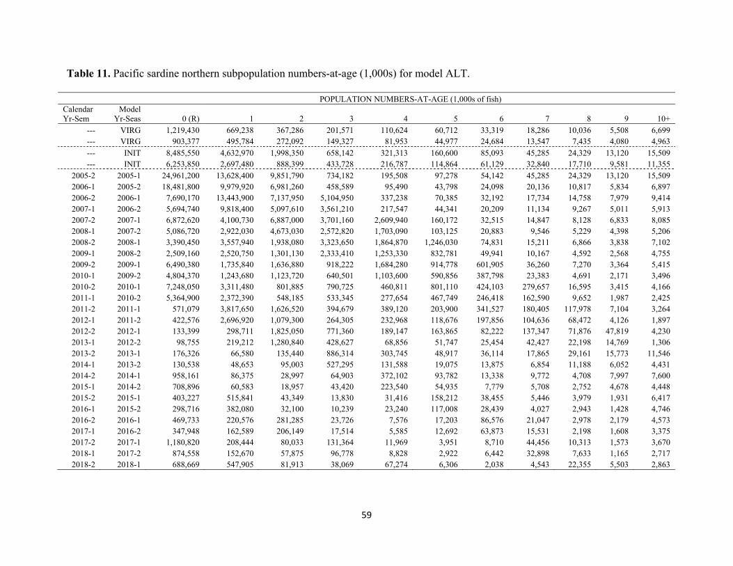
59  

Table 11. Pacific sardine northern subpopulation numbers-at-age (1,000s) for model ALT.

POPULATION NUMBERS-AT-AGE (1,000s of fish) Calendar Yr-Sem

Model Yr-Seas 0 (R) 1 2 3 4 5 6 7 8 9 10+

--- VIRG 1,219,430 669,238 367,286 201,571 110,624 60,712 33,319 18,286 10,036 5,508 6,699 --- VIRG 903,377 495,784 272,092 149,327 81,953 44,977 24,684 13,547 7,435 4,080 4,963

--- INIT 8,485,550 4,632,970 1,998,350 658,142 321,313 160,600 85,093 45,285 24,329 13,120 15,509 --- INIT 6,253,850 2,697,480 888,399 433,728 216,787 114,864 61,129 32,840 17,710 9,581 11,355

2005-2 2005-1 24,961,200 13,628,400 9,851,790 734,182 195,508 97,278 54,142 45,285 24,329 13,120 15,509 2006-1 2005-2 18,481,800 9,979,920 6,981,260 458,589 95,490 43,798 24,098 20,136 10,817 5,834 6,897 2006-2 2006-1 7,690,170 13,443,900 7,137,950 5,104,950 337,238 70,385 32,192 17,734 14,758 7,979 9,414 2007-1 2006-2 5,694,740 9,818,400 5,097,610 3,561,210 217,547 44,341 20,209 11,134 9,267 5,011 5,913 2007-2 2007-1 6,872,620 4,100,730 6,887,000 3,701,160 2,609,940 160,172 32,515 14,847 8,128 6,833 8,085 2008-1 2007-2 5,086,720 2,922,030 4,673,030 2,572,820 1,703,090 103,125 20,883 9,546 5,229 4,398 5,206 2008-2 2008-1 3,390,450 3,557,940 1,938,080 3,323,650 1,864,870 1,246,030 74,831 15,211 6,866 3,838 7,102 2009-1 2008-2 2,509,160 2,520,750 1,301,130 2,333,410 1,253,330 832,781 49,941 10,167 4,592 2,568 4,755 2009-2 2009-1 6,490,380 1,735,840 1,636,880 918,222 1,684,280 914,778 601,905 36,260 7,270 3,364 5,415 2010-1 2009-2 4,804,370 1,243,680 1,123,720 640,501 1,103,600 590,856 387,798 23,383 4,691 2,171 3,496 2010-2 2010-1 7,248,050 3,311,480 801,885 790,725 460,811 801,110 424,103 279,657 16,595 3,415 4,166 2011-1 2010-2 5,364,900 2,372,390 548,185 533,345 277,654 467,749 246,418 162,590 9,652 1,987 2,425 2011-2 2011-1 571,079 3,817,650 1,626,520 394,679 389,120 203,900 341,527 180,405 117,978 7,104 3,264 2012-1 2011-2 422,576 2,696,920 1,079,300 264,305 232,968 118,676 197,856 104,636 68,472 4,126 1,897 2012-2 2012-1 133,399 298,711 1,825,050 771,360 189,147 163,865 82,222 137,347 71,876 47,819 4,230 2013-1 2012-2 98,755 219,212 1,280,840 428,627 68,856 51,747 25,454 42,427 22,198 14,769 1,306 2013-2 2013-1 176,326 66,580 135,440 886,314 303,745 48,917 36,114 17,865 29,161 15,773 11,546 2014-1 2013-2 130,538 48,653 95,003 527,295 131,588 19,075 13,875 6,854 11,188 6,052 4,431 2014-2 2014-1 958,161 86,375 28,997 64,903 372,102 93,782 13,338 9,772 4,708 7,997 7,600 2015-1 2014-2 708,896 60,583 18,957 43,420 223,540 54,935 7,779 5,708 2,752 4,678 4,448 2015-2 2015-1 403,227 515,841 43,349 13,830 31,416 158,212 38,455 5,446 3,979 1,931 6,417 2016-1 2015-2 298,716 382,080 32,100 10,239 23,240 117,008 28,439 4,027 2,943 1,428 4,746 2016-2 2016-1 469,733 220,576 281,285 23,726 7,576 17,203 86,576 21,047 2,978 2,179 4,573 2017-1 2016-2 347,948 162,589 206,149 17,514 5,585 12,692 63,873 15,531 2,198 1,608 3,375 2017-2 2017-1 1,180,820 208,444 80,033 131,364 11,969 3,951 8,710 44,456 10,313 1,573 3,670 2018-1 2017-2 874,558 152,670 57,875 96,778 8,828 2,922 6,442 32,898 7,633 1,165 2,717 2018-2 2018-1 688,669 547,905 81,913 38,069 67,274 6,306 2,038 4,543 22,355 5,503 2,863

 

60  

Table 12. Pacific sardine northern subpopulation biomass-at-age for model ALT.

POPULATION BIOMASS-AT-AGE (mt) SUMMARY BIOMASS

Calendar Yr-Sem

Model Yr-Seas 0 1 2 3 4 5 6 7 8 9 10+ Ages 0+ Ages 1+

--- VIRG 9,146 31,387 28,097 20,963 14,082 8,852 5,331 3,121 1,791 1,015 1,297 125,083 115,938 --- VIRG 29,540 30,590 24,679 17,352 11,236 6,899 4,090 2,369 1,350 761 965 129,831 100,291

--- INIT 63,642 217,286 152,874 68,447 40,903 23,415 13,615 7,730 4,343 2,417 3,003 597,674 534,033 --- INIT 204,501 166,435 80,578 50,399 29,721 17,620 10,129 5,744 3,216 1,787 2,207 572,337 367,836

2005-2 2005-1 187,209 639,172 753,662 76,355 24,888 14,183 8,663 7,730 4,343 2,417 3,003 1,721,624 1,534,415 2006-1 2005-2 604,355 615,761 633,200 53,288 13,092 6,719 3,993 3,522 1,964 1,088 1,341 1,938,323 1,333,968 2006-2 2006-1 57,676 630,519 546,053 530,915 42,930 10,262 5,151 3,027 2,634 1,470 1,822 1,832,460 1,774,784 2007-1 2006-2 186,218 605,795 462,353 413,813 29,826 6,802 3,349 1,947 1,683 935 1,149 1,713,870 1,527,652 2007-2 2007-1 51,545 192,324 526,856 384,921 332,245 23,353 5,202 2,534 1,451 1,259 1,565 1,523,255 1,471,710 2008-1 2007-2 166,336 180,289 423,844 298,962 233,494 15,819 3,460 1,670 950 820 1,012 1,326,655 1,160,320 2008-2 2008-1 25,428 166,867 148,263 345,660 237,398 181,671 11,973 2,597 1,226 707 1,375 1,123,165 1,097,736 2009-1 2008-2 82,050 155,530 118,012 271,142 171,832 127,749 8,275 1,778 834 479 924 938,605 856,556 2009-2 2009-1 48,678 81,411 125,221 95,495 214,409 133,375 96,305 6,190 1,298 620 1,048 804,049 755,371 2010-1 2009-2 157,103 76,735 101,921 74,426 151,304 90,637 64,258 4,090 852 405 680 722,411 565,308 2010-2 2010-1 54,360 155,308 61,344 82,235 58,661 116,802 67,856 47,737 2,962 629 806 648,703 594,343 2011-1 2010-2 175,432 146,376 49,720 61,975 38,066 71,753 40,831 28,437 1,753 371 471 615,186 439,754 2011-2 2011-1 4,283 179,048 124,429 41,047 49,535 29,729 54,644 30,795 21,059 1,309 632 536,509 532,226 2012-1 2011-2 13,818 166,400 97,893 30,712 31,940 18,205 32,785 18,301 12,435 769 369 423,626 409,808 2012-2 2012-1 1,000 14,010 139,616 80,221 24,078 23,892 13,155 23,445 12,830 8,808 819 341,875 340,875 2013-1 2012-2 3,229 13,525 116,172 49,806 9,440 7,938 4,218 7,420 4,031 2,754 254 218,789 215,560 2013-2 2013-1 1,322 3,123 10,361 92,177 38,667 7,132 5,778 3,050 5,205 2,905 2,235 171,955 170,633 2014-1 2013-2 4,269 3,002 8,617 61,272 18,041 2,926 2,299 1,199 2,032 1,129 861 105,645 101,377 2014-2 2014-1 7,186 4,051 2,218 6,750 47,369 13,673 2,134 1,668 840 1,473 1,471 88,834 81,648 2015-1 2014-2 23,181 3,738 1,719 5,045 30,647 8,427 1,289 998 500 872 865 77,282 54,101 2015-2 2015-1 3,024 24,193 3,316 1,438 3,999 23,067 6,153 930 710 356 1,242 68,429 65,405 2016-1 2015-2 9,768 23,574 2,911 1,190 3,186 17,949 4,712 704 534 266 923 65,719 55,951 2016-2 2016-1 3,523 10,345 21,518 2,467 964 2,508 13,852 3,593 532 401 885 60,590 57,067 2017-1 2016-2 11,378 10,032 18,698 2,035 766 1,947 10,584 2,716 399 300 656 59,510 48,132 2017-2 2017-1 8,856 9,776 6,122 13,662 1,524 576 1,394 7,589 1,841 290 711 52,339 43,483 2018-1 2017-2 28,598 9,420 5,249 11,246 1,210 448 1,068 5,754 1,386 217 528 65,124 36,526 2018-2 2018-1 5,165 25,697 6,266 3,959 8,564 919 326 776 3,990 1,014 554 57,230 52,065

 

61  

Table 13. Spawning stock biomass (SSB) and recruitment (Recruits) estimates and asymptotic standard errors for model ALT. SSB estimates were calculated at the beginning of Season 2 of each model year (January). Recruits were age-0 fish calculated at the beginning of each model year (July).

Calendar Yr-Sem

Model Yr-Seas SSB (mt)

SSB Std Dev

Year class abundance

(1000s) Recruits Std Dev

--- VIRG-1 --- --- 1,219,430 352,606 --- VIRG-2 86,431 24,992 --- --- --- INIT-1 --- --- 8,485,550 3,887,180 --- INIT-2 310,016 85,120 --- ---

2005-2 2005-1 --- --- 24,961,200 --- 2006-1 2005-2 1,059,660 77,048 --- --- 2006-2 2006-1 --- --- 7,690,170 899,841 2007-1 2006-2 1,204,400 77,125 --- --- 2007-2 2007-1 --- --- 6,872,620 759,179 2008-1 2007-2 1,022,610 64,721 --- --- 2008-2 2008-1 --- --- 3,390,450 510,566 2009-1 2008-2 764,224 47,354 --- --- 2009-2 2009-1 --- --- 6,490,380 649,386 2010-1 2009-2 530,481 33,318 --- --- 2010-2 2010-1 --- --- 7,248,050 773,373 2011-1 2010-2 389,116 26,270 --- --- 2011-2 2011-1 --- --- 571,079 141,498 2012-1 2011-2 323,330 25,503 --- --- 2012-2 2012-1 --- --- 133,399 47,950 2013-1 2012-2 190,005 22,097 --- --- 2013-2 2013-1 --- --- 176,326 61,904 2014-1 2013-2 95,658 16,040 --- --- 2014-2 2014-1 --- --- 958,161 279,848 2015-1 2014-2 54,402 11,186 --- --- 2015-2 2015-1 --- --- 403,227 183,415 2016-1 2015-2 46,439 9,326 --- --- 2016-2 2016-1 --- --- 469,733 178,163 2017-1 2016-2 42,441 8,317 --- --- 2017-2 2017-1 --- --- 1,180,820 911,442 2018-1 2017-2 35,075 8,394 --- ---

 

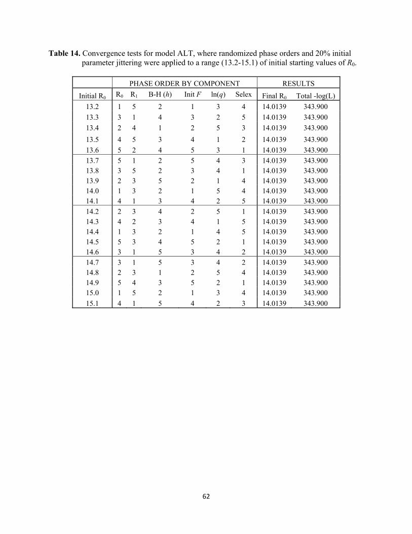
62  

Table 14. Convergence tests for model ALT, where randomized phase orders and 20% initial parameter jittering were applied to a range (13.2-15.1) of initial starting values of R0.

PHASE ORDER BY COMPONENT RESULTS

Initial R0 R0 R1 B-H (h) Init F ln(q) Selex Final R0 Total -log(L)

13.2 1 5 2 1 3 4 14.0139 343.900

13.3 3 1 4 3 2 5 14.0139 343.900

13.4 2 4 1 2 5 3 14.0139 343.900

13.5 4 5 3 4 1 2 14.0139 343.900

13.6 5 2 4 5 3 1 14.0139 343.900

13.7 5 1 2 5 4 3 14.0139 343.900 13.8 3 5 2 3 4 1 14.0139 343.900 13.9 2 3 5 2 1 4 14.0139 343.900 14.0 1 3 2 1 5 4 14.0139 343.900 14.1 4 1 3 4 2 5 14.0139 343.900

14.2 2 3 4 2 5 1 14.0139 343.900 14.3 4 2 3 4 1 5 14.0139 343.900 14.4 1 3 2 1 4 5 14.0139 343.900 14.5 5 3 4 5 2 1 14.0139 343.900 14.6 3 1 5 3 4 2 14.0139 343.900

14.7 3 1 5 3 4 2 14.0139 343.900 14.8 2 3 1 2 5 4 14.0139 343.900 14.9 5 4 3 5 2 1 14.0139 343.900 15.0 1 5 2 1 3 4 14.0139 343.900

15.1 4 1 5 4 2 3 14.0139 343.900

 

63  

Table 15. Harvest control rules for the update model ALT. Note that the SSB was projected to be 36,651 mt (SD=15,867 mt; CV=43.3%) in January 2019, so the corresponding Sigma for calculating P-star buffers is 0.415 rather than the default value (0.36) for Tier 1 assessments.

OFL = BIOMASS * E MSY * DISTRIBUTION; where E MSY is bounded 0.00 to 0.25

ABCP-star = BIOMASS * BUFFERP-star * E MSY * DISTRIBUTION; where E MSY is bounded 0.00 to 0.25

HG = (BIOMASS - CUTOFF) * FRACTION * DISTRIBUTION; where FRACTION is E MSY bounded 0.05 to 0.20

BIOMASS (ages 1+, mt) 52,065P-star 0.45 0.40 0.35 0.30 0.25 0.20 0.15 0.10 0.05

ABC Buffer(Sigma 0.415) 0.94924 0.90030 0.85237 0.80462 0.75609 0.70548 0.65074 0.58787 0.50568

ABC BufferTier 2 0.91350 0.83326 0.75773 0.68553 0.61531 0.54555 0.47415 0.39744 0.30596

CalCOFI SST (2015-2017) 16.6435E MSY 0.25

FRACTION 0.20CUTOFF (mt) 150,000

DISTRIBUTION (U.S.) 0.87

OFL = 11,324

ABCTier 1 = 10,749 10,195 9,652 9,112 8,562 7,989 7,369 6,657 5,726

ABCTier 2 = 10,345 9,436 8,581 7,763 6,968 6,178 5,369 4,501 3,465

HG = 0

Harvest Control Rule Values (MT)

Harvest Control Rule Formulas

Harvest Formula Parameters

 

64  

Table 16. CalCOFI annual and three-year average sea surface temperatures (SST, °C) since 1984. Three-year average SST is used to calculate EMSY in the harvest control rules.

Calendar

year CalCOFI

Annual SST CalCOFI 3-yr average SST

1984 16.3533 --- 1985 15.7605 --- 1986 15.9823 16.0320 1987 16.2973 16.0134 1988 15.7851 16.0216 1989 15.4632 15.8485 1990 15.9946 15.7476 1991 15.7998 15.7525 1992 16.7028 16.1657 1993 16.4182 16.3069 1994 16.4762 16.5324 1995 15.9241 16.2729 1996 16.3252 16.2419 1997 16.6950 16.3148 1998 16.7719 16.5973 1999 15.2843 16.2504 2000 15.7907 15.9490 2001 15.5535 15.5429 2002 14.9414 15.4285 2003 16.0328 15.5092 2004 15.8849 15.6197 2005 15.4585 15.7920 2006 15.9157 15.7530 2007 15.1543 15.5095 2008 15.2724 15.4475 2009 15.3583 15.2617 2010 15.5520 15.3942 2011 15.5618 15.4907 2012 15.2939 15.4692 2013 14.9097 15.2551 2014 14.1932 14.7989 2015 17.4765 15.5265 2016 16.3300 15.9999 2017 16.1240 16.6435

 

65  

FIGURES

 

66  

Figure 1. Distribution of the northern subpopulation of Pacific sardine, primary commercial

fishing areas, and modeled fleets.

 

67  

Figure 2. U.S. Pacific sardine harvest guidelines or acceptable catch limits and landings since

the onset of federal management.

 

68  

Figure 3. Pacific sardine NSP landings (mt) by major fishing region.

 

69  

Figure 4. Length-at-age by sex from NSP fishery samples (1993-2013; Hill et al. 2014),

indicating lack of sexually dimorphic growth. Box symbols indicate median and quartile ranges for the raw data.

MF

SEX$

0 2 4 6 8 10 12

AGE_SS

0

10

20

30S

L_

CM

 

70  

Figure 5. Empirical weight-at-age time series for the MEXCAL fleet in seasons 1 and 2.

 

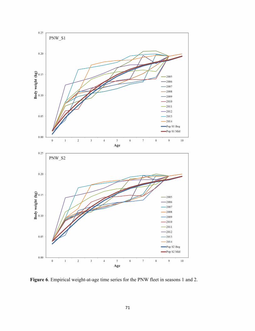
71  

Figure 6. Empirical weight-at-age time series for the PNW fleet in seasons 1 and 2.

 

72  

Figure 7. Empirical weight-at-age time series for the AT survey in seasons 1 and 2.

 

73  

Figure 8. Population body weights-at-age and SSB-at-age applied in model ALT. Population

body weights-at-age are provided at the beginning and middle of seasons 1 and 2, and fecundity*maturity-at-age is used to calculate SSB at the beginning of season 2.

 

74  

Figure 9. Pacific sardine NSP landings (mt) by fleet, model year and semester as used in model

ALT.

 

75  

Figure 10. Age composition time series for the MEXCAL fleet in seasons 1 (upper) and 2

(lower). N represents input sample sizes.

 

76  

Figure 11. Age composition time series for the PNW fleet in season 1. N represents input sample

sizes.

 

77  

Figure 12a. Length (upper panel) and age-composition (lower panel) time series for the AT

survey. N represents input sample sizes. Age compositions were derived from length compositions using season-specific age-length keys.

 

78  

Figure 12b. Aggregate age-length key derived from summer AT survey samples collected from

2006-2016 (upper and lower panels). Summer 2017 age data are overlaid in the lower panel (red dots). Survey age compositions were derived from length compositions using season-specific age-length keys, excluding the anomalous 2017 data.

 

79  

Figure 13. Laboratory- and year-specific ageing errors applied in model ALT.

 

80  

Figure 14. Results from the AT survey for summer 2017. A map of the a) distribution of 38-kHz integrated backscattering coefficients (sA, m2 nmi-2; averaged over 2000-m distance intervals and from 5 to 70-m deep) ascribed to CPS; b) CUFES egg density (eggs m-3) for anchovy, sardine, and jack mackerel; and c) proportions of CPS species in trawls (black points indicate trawls with no CPS).

 

81  

Figure 15. Sardine biomass densities versus stratum (Table 6) estimated in the AT survey for summer 2017. Numbers in red represent the locations of trawl clusters with at least one sardine. Strata 4, 5 and 6 are coastal strata surveyed by FV Lisa Marie off Oregon and Washington.

 

82  

Figure 16. Estimated sardine abundance (top row) and biomass (bottom row) by length (left column) and age (right column) for the entire summer 2017 survey area (see Figure 15).

 

83  

Figure 17. Time-series of Pacific sardine biomass with respective 95% confidence intervals as

estimated by acoustic-trawl (AT) surveys. The biomass in July 2018 was projected based on the summer 2017 AT biomass and the expected recruitment using the ALT model’s S-R relationship.

 

84  

Figure 18. Age-selectivity patterns for model ALT.

 

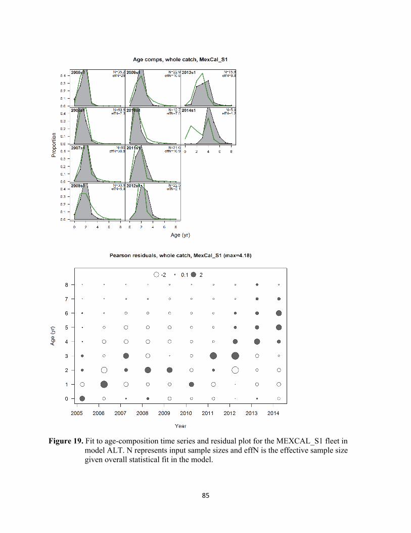
85  

Figure 19. Fit to age-composition time series and residual plot for the MEXCAL_S1 fleet in

model ALT. N represents input sample sizes and effN is the effective sample size given overall statistical fit in the model.

 

86  

Figure 20. Fit to age-composition time series and residual plot for the MEXCAL_S2 fleet in

model ALT. N represents input sample sizes and effN is the effective sample size given overall statistical fit in the model.

 

87  

Figure 21. Fit to age-composition time series and residual plot for the PNW fleet in model ALT.

N represents input sample sizes and effN is the effective sample size given overall statistical fit in the model.

 

88  

Figure 22. Fit to age-composition time series and residual plot for the AT survey for model

ALT. N represents input sample sizes and effN is the effective sample size given overall statistical fit in the model.

 

89  

Figure 23. Fit to the AT survey abundance index in arithmetic (upper panel) and log (lower

panel) scales for model ALT. Q=1.15 (estimated).

 

90  

Figure 24. Estimated stock-recruitment (Beverton-Holt) relationship for model ALT. Steepness

is estimated (h=0.322). Year labels represent year of SSB producing the subsequent year class.

Figure 25. Recruitment deviations and standard errors (σR = 0.75) for model ALT. Year labels

represent year of SSB producing the subsequent year class.

 

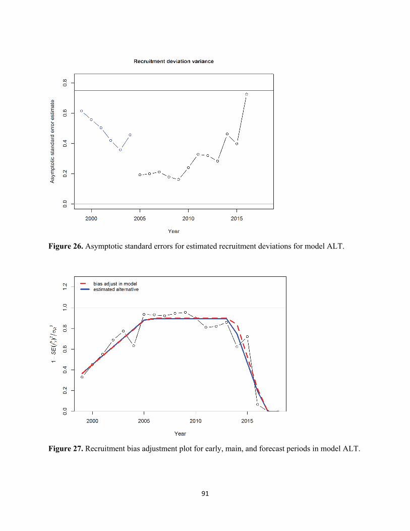
91  

Figure 26. Asymptotic standard errors for estimated recruitment deviations for model ALT.

Figure 27. Recruitment bias adjustment plot for early, main, and forecast periods in model ALT.

 

92  

Figure 28. Spawning stock biomass time series (±95% CI) for model ALT.

 

93  

Figure 29. Estimated stock biomass (age 1+ fish, mt) time series for the AT survey and model

ALT.

 

94  

Figure 30. Recruit (age-0 fish, billions) abundance time series (±95% CI) for model ALT.

 

95  

Figure 31. Instantaneous fishing mortality (apical F) time series for model ALT. Note that high

F values for the PNW fleet reflect rates for fishes ages 6 and older.

Figure 32. Annual exploitation rates (CY landings / July total biomass) for model ALT.

 

96  

Figure 33. Retrospective analyses of stock biomass (age 1+) for model ALT.

 

97  

Figure 34. Estimated stock biomass (age 1+ fish, mt, upper panel) and recruitment (lower panel)

time series for model ALT and past assessment model used for management.

 

98  

Figure 35. CalCOFI sea surface temperatures (SST, °C, upper panel) and calculated EMSY values

(lower panel).

 

99  

APPENDIX A

SS INPUT FILES FOR MODEL ALT

STARTER.SS # Pacific sardine stock assessment (2018-19) # P.R. Crone, K.T. Hill, J.P. Zwolinski (Jan 2018) # Model ALT # SS model (ver. 3.24aa) # Starter file # ALT_18.dat ALT_18.ctl 0 # 0=use init values in control file; 1=use ss3.par 1 # Run display detail (0,1,2) 2 # Detailed age-structured reports in REPORT.SSO: (0,1,2) 1 # Write detailed checkup.sso file (0,1) 3 # Write parm values to ParmTrace.sso (0=no,1=good,active; 2=good,all; 3=every_iter,all_parms; 4=every,active) 2 # Write to cumreport.sso (0=no, 1=like&timeseries, 2=add survey fits) 0 # Include prior_like for non-estimated parameters (0,1) 1 # Use soft boundaries to aid convergence: (0,1) 1 # Number of datafiles to produce: 1st is input, 2nd is estimates, 3rd and higher are bootstrap 10 # Turn off estimation for parameters entering after this phase 10 # MCeval burn interval 2 # MCeval thin interval 0.05 # Jitter initial parm value by this fraction -1 # Min yr for sdreport outputs (-1 for styr) -2 # Max yr for sdreport outputs (-1 for endyr; -2 for endyr+Nforecastyrs 0 # N individual STD years # Vector of year values 0.00001 # Final convergence criteria (e.g., 1.0e-05) 0 # Retrospective year relative to end year (e.g. -4) 1 # Min age for calc of summary biomass 1 # Depletion basis: denom is: 0=skip; 1=rel X*B0; 2=rel X*Bmsy; 3=rel X*B_styr 1 # Fraction (X) for depletion denominator (e.g. 0.4) 4 # SPR_report_basis: 0=skip; 1=(1-SPR)/(1-SPR_tgt); 2=(1-SPR)/(1-SPR_MSY); 3=(1-SPR)/(1-SPR_Btarget); 4=rawSPR 4 # F_report_units: 0=skip; 1=exploitation(Bio); 2=exploitation(Num); 3=sum(Frates); 4=true F for range of ages 0 8 # Min and max age over which average F will be calculated with F_reporting=4 2 # F_report_basis: 0=raw; 1=F/Fspr; 2=F/Fmsy ; 3=F/Fbtgt 999 # End of file

FORECAST.SS # Pacific sardine stock assessment (2018-19) # P.R. Crone, K.T. Hill, J.P. Zwolinski (Jan 2018) # Model ALT # SS model (ver. 3.24aa) # Forecast file # # Note: for all year entries except rebuilder, enter either: actual year, -999 for styr, 0 for endyr, neg number

for relative endyr 1 #_Benchmarks: 0=skip, 1=calc F_spr,F_btgt,F_msy 2 #_MSY: 1= set to F(SPR), 2=calc F(MSY), 3=set to F(Btgt), 4=set to F(endyr) 0.4 #_SPR target (e.g., 0.40) 0.4 #_Biomass target (e.g., 0.40) # Bmark_years: beg_bio, end_bio, beg_selex, end_selex, beg_relF, end_relF (enter actual year, or values of 0 or

-integer to be rel. endyr) 0 0 0 0 0 0 1 # Bmark_relF_basis: 1 = use year range; 2 = set relF same as forecast below 1 # Forecast: 0=none; 1=F(SPR); 2=F(MSY) 3=F(Btgt); 4=Ave F (uses first-last relF yrs); 5=input annual F scalar 1 # N forecast years 0 # F scalar (only used for Do_Forecast==5) # Fcast_years: beg_selex, end_selex, beg_relF, end_relF (enter actual year, or values of 0 or -integer to be

rel. endyr) 0 0 0 0 1 # Control rule method (1=catch=f(SSB) west coast, 2=F=f(SSB) ) 0.5 # Control rule Biomass level for constant F (as frac of Bzero, e.g. 0.40); (Must be > the no F level below) 0.1 # Control rule Biomass level for no F (as frac of Bzero, e.g. 0.10) 0.75 # Control rule target as fraction of Flimit (e.g. 0.75) 3 # N forecast loops 3 # First forecast loop with stochastic recruitment 0 # Forecast loop control #3 (reserved for future bells&whistles) 0 # Forecast loop control #4 (reserved for future bells&whistles)

 

100  

0 # Forecast loop control #5 (reserved for future bells&whistles) 2020 # FirstYear for caps and allocations (should be after years with fixed inputs) 0 # Stddev of log(realized catch/target catch) in forecast (set value>0.0 to cause active impl_error) 0 # Do West Coast gfish rebuilder output (0/1) 0 # Rebuilder: first year catch could have been set to zero (Ydecl)(-1 to set to 1999) 0 # Rebuilder: year for current age structure (Yinit) (-1 to set to endyear+1) 1 # Fleet relative F: 1=use first-last alloc year, 2=read seas(row) x fleet(col) below # Note: fleet allocation is used directly as average F if Do_Forecast=4 2 # Basis for forecast catch tuning and for forecast catch caps and allocation: 2=deadbio, 3=retainbio,

5=deadnum, 6=retainnum # Conditional input if relative F option=2 # Fleet relative F: rows are seasons, columns are fleets # Fleet: MexCal_S1 MexCal_S2 PNW # 0 0 0 # S1 # 0 0 0 # S2 # Max total catch by fleet (-1 to have no max): must enter value for each fleet -1 -1 -1 # Max total catch by area (-1 to have no max): must enter value for each fleet -1 # Fleet assignment to allocation group (enter group ID# for each fleet, 0 for not included in an alloc group) 0 0 0 # Conditional on >1 allocation group # Allocation fraction for each of: 0 allocation groups # No allocation groups 6 # Number of forecast catch levels to input (or else calculate catch from forecast F) 2 # Basis for input forecast catch: 2=dead catch, 3=retained catch, 99 = input Hrate(F) with units that are from

fishery units # Input fixed catch values # Year Season Fleet Catch/F 2018 1 1 378.20 2018 2 1 0.00 2018 1 2 0.00 2018 2 2 8081.11 2018 1 3 1.20 2018 2 3 0.10 999 # End of file

ALT.DAT # Pacific sardine stock assessment (2018-19) # P.R. Crone, K.T. Hill, J.P. Zwolinski (Jan 2018) # Model ALT # SS model (ver. 3.24aa) # Data file # 2005 # Start year 2017 # End year (ADVANCED ONE YEAR; FORECAST=2018-19) 2 # N_seasons 6 6 # Months per season (2 semesters per fishing year) 2 # Spawning season (Spring semester) 3 # N_fleets 1 # N_surveys 1 # N_areas MexCal_S1%MexCal_S2%PNW%AT_Survey 0.5 0.5 0.5 0.75 # Survey timing in season 1 1 1 1 # Area assignments for each fishery/survey 1 1 1 # Units of catch: 1=biomass, 2=number 0.05 0.05 0.05 # SE of log(catch), only used for initial equilibrium catch and for Fmethod=2-3 1 # N_genders 10 # N_ages 1000 0 0 # Initial equilibrium catch for each fishery 26 # N_lines of catch to read # Catch biomass(mt): columns are fisheries, year, season # LANDINGS (FINAL 2016 AND PRELIM 2017) 13802.99 0.00 54152.62 2005 1 0.00 30364.20 101.70 2005 2 20726.23 0.00 41220.90 2006 1 0.00 39900.28 0.00 2006 2 46228.11 0.00 48237.10 2007 1 0.00 42910.05 0.00 2007 2 30249.18 0.00 39800.10 2008 1 0.00 41198.49 0.00 2008 2 14044.87 0.00 44841.15 2009 1 0.00 31146.46 1369.73 2009 2 11273.97 0.00 54085.91 2010 1

 

101  

0.00 27267.62 0.09 2010 2 24871.40 0.00 39750.49 2011 1 0.00 23189.90 5805.63 2011 2 1528.37 0.00 91425.63 2012 1 0.00 13884.90 1570.78 2012 2 921.56 0.00 57217.96 2013 1 0.00 5625.03 908.01 2013 2 1830.92 0.00 15216.82 2014 1 0.00 727.71 2193.87 2014 2 6.13 0.00 66.28 2015 1 0.00 185.82 1.40 2015 2 283.54 0.00 87.90 2016 1 0.00 8081.11 0.10 2016 2 378.20 0.00 1.20 2017 1 0.00 8081.11 0.10 2017 2 # 16 #_N_cpue_and_surveyabundance_observations #_Units: 0=numbers; 1=biomass; 2=F #_Errtype: -1=normal; 0=lognormal; >0=T #_Fleet Units Errtype 1 1 0 # MexCal_S1 2 1 0 # MexCal_S2 3 1 0 # PNW 4 1 0 # ATM # Year season index obs error 2005 2 4 1947063 0.30 # ATM_0604 2007 2 4 751075 0.09 # ATM_0804 2009 2 4 357006 0.41 # ATM_1004 2010 2 4 493672 0.30 # ATM_1104 2011 2 4 469480 0.28 # ATM_1204 2012 2 4 305146 0.24 # ATM_1304 2013 2 4 35339 0.38 # ATM_1404 2014 2 4 29048 0.29 # ATM_1504 2015 2 4 83030 0.47 # ATM_1604 2008 1 4 801000 0.30 # ATM_0807 2012 1 4 340831 0.33 # ATM_1207 2013 1 4 313746 0.27 # ATM_1307 2014 1 4 26280 0.63 # ATM_1407 2015 1 4 15870 0.70 # ATM_1507 2016 1 4 78770 0.51 # ATM_1607 2017 1 4 36644 0.29 # ATM_1707 # 0 # N_fleets with discard # Discard units: 1=same_as_catch units (bio/num), 2=fraction, 3=numbers # Discard error type: >0 for DF of T-dist(read CV below), 0 for normal with CV, -1 for normal with se, -2 for

lognormal # Fleet discard units and error type 0 # N_discard obs # Year season index obs error # 0 # N_meanbodywt obs 100 # DF for_meanbodywt t-distribution likelihood # 2 # Length bin method: 1=use databins; 2=generate from binwidth,min,max below; 3=read vector 0.5 # Bin width for population size composition 8 # Minimum size in the population (lower edge of first bin and size at age 0) 30 # Maximum size in the population (lower edge of last bin) -0.0001 # Composition tail compression 0.0001 # Add to composition 0 # Combine males into females at or below this bin number 39 # N_length bins 9 9.5 10 10.5 11 11.5 12 12.5 13 13.5 14 14.5 15 15.5 16 16.5 17 17.5 18 18.5 19 19.5 20 20.5 21 21.5 22 22.5 23

23.5 24 24.5 25 25.5 26 26.5 27 27.5 28 16 # N_length obs # Year Season Fleet/Survey Gender Part Nsamp Datavector(female-male) 2005 2 -4 0 0 10.00 0.00000000 0.00000000 0.00000000 0.00000000 0.00000000

0.00000000 0.00000000 0.00000000 0.00270862 0.00270862 0.00000000 0.00000000 0.01100873 0.01100873 0.12353364 0.12353364 0.06453880 0.06453880 0.15773170 0.15773170 0.06426980 0.06426980 0.05009669 0.05009669 0.01516183 0.01516183 0.00505394 0.00505394 0.00000000 0.00000000 0.00168465 0.00168465 0.00336930 0.00336930 0.00168465 0.00000000 0.00000000 0.00000000 0.00000000

2007 2 -4 0 0 12.00 0.00000000 0.00000000 0.00000000 0.00000000 0.00000000 0.00000000 0.00000000 0.00000000 0.00000000 0.00000000 0.00000000 0.00000000 0.00000000 0.00000000 0.01871052 0.01871052 0.04456086

 

102  

0.04456086 0.07885461 0.07885461 0.07720993 0.07720993 0.09196321 0.09196321 0.10803940 0.10803940 0.06881783 0.06881783 0.00321240 0.00321240 0.00825866 0.00825866 0.00037258 0.00037258 0.00000000 0.00000000 0.00000000 0.00000000 0.00000000

2009 2 -4 0 0 19.00 0.00000000 0.00000000 0.00000000 0.00000000 0.00071913 0.00071913 0.00036184 0.00036184 0.00000000 0.00000000 0.00121512 0.00121512 0.00265337 0.00265337 0.00332081 0.00332081 0.00555546 0.00555546 0.00224440 0.00224440 0.00833426 0.00833426 0.05506318 0.05506318 0.17107802 0.17107802 0.16580872 0.16580872 0.06954074 0.06954074 0.01153821 0.01153821 0.00243023 0.00243023 0.00027301 0.00000000 0.00000000 0.00000000 0.00000000

2010 2 -4 0 0 18.00 0.00000000 0.00000000 0.00000000 0.00000000 0.00000000 0.00000000 0.00000449 0.00000449 0.00000000 0.00000000 0.00000000 0.00000000 0.00015121 0.00015121 0.08020558 0.08020558 0.22135962 0.22135962 0.08918809 0.08918809 0.04535153 0.04535153 0.00957193 0.00957193 0.00287216 0.00287216 0.01710648 0.01710648 0.02239309 0.02239309 0.00960401 0.00960401 0.00139900 0.00139900 0.00158562 0.00000000 0.00000000 0.00000000 0.00000000

2011 2 -4 0 0 12.00 0.00000000 0.00000000 0.00000000 0.00000000 0.00000000 0.00000000 0.00000000 0.00000000 0.00000000 0.00000000 0.00000000 0.00000000 0.00000000 0.00000000 0.00000000 0.00000000 0.00966230 0.00966230 0.00000000 0.00000000 0.00874343 0.00874343 0.09109599 0.09109599 0.11348639 0.11348639 0.05587484 0.05587484 0.10595060 0.10595060 0.08715280 0.08715280 0.02797210 0.02797210 0.00006153 0.00006153 0.00000000 0.00000000 0.00000000

2012 2 -4 0 0 18.00 0.00000000 0.00000000 0.00000000 0.00000000 0.00000000 0.00000000 0.00000000 0.00000000 0.00000000 0.00000000 0.00000000 0.00000000 0.00000000 0.00000000 0.00000000 0.00000000 0.00000000 0.00000000 0.00087027 0.00087027 0.00043514 0.00043514 0.01933857 0.01933857 0.15265050 0.15265050 0.18642185 0.18642185 0.07407997 0.07407997 0.04749947 0.04749947 0.00758276 0.00758276 0.01112147 0.01112147 0.00000000 0.00000000 0.00000000

2013 2 -4 0 0 4.00 0.00000000 0.00000000 0.00000000 0.00000000 0.00000000 0.00000000 0.00000000 0.00000000 0.00000000 0.00000000 0.00000000 0.00000000 0.00000000 0.00000000 0.00000000 0.00000000 0.00000000 0.00000000 0.00000000 0.00000000 0.00000000 0.00000000 0.00000000 0.00000000 0.00000000 0.00000000 0.03553942 0.03553942 0.32050317 0.32050317 0.10057675 0.10057675 0.04338066 0.04338066 0.00000000 0.00000000 0.00000000 0.00000000 0.00000000

2014 2 -4 0 0 6.00 0.00000000 0.00000000 0.00000000 0.00000000 0.00000000 0.00000000 0.00000000 0.00000000 0.00000000 0.00000000 0.00000000 0.00000000 0.00000000 0.00000000 0.00000000 0.00000000 0.00195881 0.00195881 0.00000000 0.00000000 0.04068968 0.04068968 0.12361069 0.12361069 0.00000000 0.00000000 0.00000000 0.00000000 0.01110877 0.01110877 0.18187444 0.18187444 0.12041276 0.12041276 0.02034484 0.02034484 0.00000000 0.00000000 0.00000000

2015 2 -4 0 0 8.00 0.00000000 0.00000000 0.00000000 0.00000000 0.00003149 0.00003149 0.00020758 0.00020758 0.02511719 0.02511719 0.11809357 0.11809357 0.08903510 0.08903510 0.02052566 0.02052566 0.00228070 0.00228070 0.00000000 0.00000000 0.02749376 0.02749376 0.03859413 0.03859413 0.02441912 0.02441912 0.00723552 0.00723552 0.00343672 0.00343672 0.04204884 0.04204884 0.06323913 0.06323913 0.03824149 0.03824149 0.00000000 0.00000000 0.00000000

2008 1 -4 0 0 27.00 0.01700544 0.01700544 0.02210707 0.02210707 0.00680218 0.00680218 0.00000000 0.00000000 0.00000000 0.00000000 0.00000000 0.00000000 0.00000000 0.00000000 0.00680218 0.00680218 0.02009720 0.02009720 0.02164783 0.02164783 0.08951514 0.08951514 0.10939327 0.10939327 0.14029251 0.14029251 0.05385909 0.05385909 0.01118376 0.01118376 0.00129435 0.00129435 0.00000000 0.00000000 0.00000000 0.00000000 0.00000000 0.00000000 0.00000000

2012 1 -4 0 0 26.00 0.00000000 0.00000000 0.00000000 0.00000000 0.00000000 0.00000000 0.00000000 0.00000000 0.00000000 0.00000000 0.00000000 0.00000000 0.00000000 0.00000000 0.00000000 0.00000000 0.00000000 0.00000000 0.00035481 0.00035481 0.00193496 0.00193496 0.13636929 0.13636929 0.21595031 0.21595031 0.06930702 0.06930702 0.04528789 0.04528789 0.02760803 0.02760803 0.00294741 0.00294741 0.00024028 0.00024028 0.00000000 0.00000000 0.00000000

2013 1 -4 0 0 23.00 0.00000000 0.00000000 0.00000000 0.00000000 0.00000000 0.00000000 0.00000000 0.00000000 0.00000000 0.00000000 0.00000000 0.00000000 0.00000000 0.00000000 0.00000000 0.00000000 0.00000000 0.00000000 0.00000000 0.00000000 0.00000000 0.00000000 0.00002651 0.00002651 0.02839681 0.02839681 0.20512511 0.20512511 0.17157365 0.17157365 0.07299605 0.07299605 0.02026224 0.02026224 0.00161961 0.00161961 0.00000000 0.00000000 0.00000000

2014 1 -4 0 0 7.00 0.00204979 0.00204979 0.00000000 0.00000000 0.00000000

 

103  

0.00000000 0.00000000 0.00000000 0.00000000 0.00000000 0.00000369 0.00000369 0.00000000 0.00000000 0.00000000 0.00000000 0.00000000 0.00000000 0.00000000 0.00000000 0.00000000 0.00000000 0.00000000 0.00000000 0.00000000 0.00000000 0.00903077 0.00903077 0.15522242 0.15522242 0.26099332 0.26099332 0.06138772 0.06138772 0.01131228 0.01131228 0.00000000 0.00000000 0.00000000

2015 1 -4 0 0 17.00 0.40403690 0.40403690 0.00000000 0.00000000 0.00000000 0.00000000 0.00000000 0.00000000 0.00000000 0.00000000 0.00000000 0.00000000 0.00000000 0.00000000 0.00000380 0.00000380 0.00000000 0.00000000 0.00000000 0.00000000 0.00000000 0.00000000 0.00187125 0.00187125 0.00561487 0.00561487 0.00192622 0.00192622 0.00374361 0.00374361 0.02701399 0.02701399 0.04906669 0.04906669 0.00666849 0.00666849 0.00005418 0.00005418 0.00000000

2016 1 -4 0 0 12.00 0.02582573 0.02582573 0.00516515 0.00516515 0.00000000 0.00000000 0.00516515 0.00516515 0.00019948 0.00019948 0.00080251 0.00080251 0.00518937 0.00518937 0.03520717 0.03520717 0.15997810 0.15997810 0.08620133 0.08620133 0.16424753 0.16424753 0.00260972 0.00260972 0.00033790 0.00033790 0.00115483 0.00115483 0.00100394 0.00100394 0.00189810 0.00189810 0.00277042 0.00277042 0.00195391 0.00195391 0.00028966 0.00028966 0.00000000

2017 1 -4 0 0 19.00 0.08906876 0.08906876 0.08193735 0.08193735 0.00000000 0.00000000 0.00000000 0.00000000 0.00000000 0.00000000 0.00000000 0.00000000 0.00000000 0.00000000 0.00000000 0.00000000 0.00003280 0.00003280 0.00970304 0.00970304 0.00427304 0.00427304 0.03977915 0.03977915 0.07175837 0.07175837 0.11432394 0.11432394 0.05564421 0.05564421 0.00879495 0.00879495 0.00900182 0.00900182 0.01463235 0.01463235 0.00105022 0.00105022 0.00000000

# 9 # N_age bins

0 1 2 3 4 5 6 7 8

6 # N_ageerror definitions

# 0.5 1.5 2.5 3.5 4.5 5.5 6.5 7.5 8.5 9.5 10.5 # 1_CA_1981-06 0.2832 0.2832 0.289 0.8009 0.8038 0.9597 1.1156 1.2715 1.4274 1.5833 1.7392 # 1_CA_1981-06 0.5 1.5 2.5 3.5 4.5 5.5 6.5 7.5 8.5 9.5 10.5 # 2_CA_2007 0.2539 0.2539 0.3434 0.9205 0.9653 1.1743 1.3832 1.5922 1.8011 2.0101 2.219 # 2_CA_2007 0.5 1.5 2.5 3.5 4.5 5.5 6.5 7.5 8.5 9.5 10.5 # 3_CA_2008-09 0.4032 0.4032 0.4995 0.58 0.6902 0.8246 0.9727 1.0165 1.1144 1.2123 1.3102 # 3_CA_2008-09 0.5 1.5 2.5 3.5 4.5 5.5 6.5 7.5 8.5 9.5 10.5 # 4_CA_2010-13 0.2825 0.2825 0.2955 0.3125 0.3347 0.3637 0.4017 0.4046 0.4245 0.4445 0.4645 # 4_CA_2010-13 0.5 1.5 2.5 3.5 4.5 5.5 6.5 7.5 8.5 9.5 10.5 # 5_ORWA_all 0.26655 0.30145 0.3149 0.3615 0.3847 0.3961 0.4018 0.4047 0.4061 0.4352 0.4487 # 5_ORWA_all 0.5 1.5 2.5 3.5 4.5 5.5 6.5 7.5 8.5 9.5 10.5 # 6_CalCOFI_C 0.5386 0.5386 0.7547 0.8341 0.8634 0.8741 0.8781 0.8796 0.8801 0.8801 0.8801 # 6_CalCOFI_C # 46 # N_age composition obs 3 # Length bin method: 1=poplenbins, 2=datalenbins, 3=lengths -1 # Combine males into females at or below this bin number # Age comps (CAAL) # Year Season Fleet/Survey Gender Part Ageerr Lbin_lo Lbin_hi Nsamp datavector(female-male) 2005 1 1 0 0 1 -1 -1 35.24 0.09102697 0.26552164 0.59466314 0.04284618

0.00412282 0.00121284 0.00060642 0.00000000 0.00000000 2006 1 1 0 0 1 -1 -1 69.76 0.00908783 0.64539166 0.30295669 0.04256381

0.00000000 0.00000000 0.00000000 0.00000000 0.00000000 2007 1 1 0 0 2 -1 -1 86.00 0.01357889 0.16055166 0.64593872 0.17061145

0.00931929 0.00000000 0.00000000 0.00000000 0.00000000 2008 1 1 0 0 3 -1 -1 30.84 0.06153622 0.26350954 0.58776778 0.07218948

0.01499698 0.00000000 0.00000000 0.00000000 0.00000000 2009 1 1 0 0 3 -1 -1 22.88 0.00349661 0.21120316 0.63114846 0.14041369

0.01373808 0.00000000 0.00000000 0.00000000 0.00000000 2010 1 1 0 0 4 -1 -1 12.68 0.01577287 0.79179811 0.16719243 0.02523659

0.00000000 0.00000000 0.00000000 0.00000000 0.00000000 2011 1 1 0 0 4 -1 -1 21.64 0.00000000 0.32278273 0.47187076 0.19905465

0.00629186 0.00000000 0.00000000 0.00000000 0.00000000 2012 1 1 0 0 4 -1 -1 22.32 0.00335775 0.10053293 0.44773547 0.37325638

0.05790999 0.01147166 0.00573583 0.00000000 0.00000000 2013 1 1 0 0 4 -1 -1 15.84 0.01132400 0.02443363 0.25675788 0.29354382

0.33484537 0.04608165 0.01688430 0.00806468 0.00806468 2014 1 1 0 0 4 -1 -1 5.92 0.00009926 0.00000451 0.00000451 0.08063643

0.53220043 0.28222750 0.08870007 0.01612729 0.00000000 2005 2 2 0 0 1 -1 -1 89.04 0.53994582 0.36702223 0.08416083 0.00500806

0.00132284 0.00090732 0.00072560 0.00045366 0.00045366

 

104  

2006 2 2 0 0 1 -1 -1 105.16 0.20172661 0.63015996 0.15000726 0.01740041 0.00070577 0.00000000 0.00000000 0.00000000 0.00000000

2007 2 2 0 0 2 -1 -1 67.44 0.42021952 0.43386305 0.10589809 0.03396340 0.00544372 0.00061223 0.00000000 0.00000000 0.00000000

2008 2 2 0 0 3 -1 -1 39.76 0.19862191 0.52834154 0.21532639 0.05558720 0.00212296 0.00000000 0.00000000 0.00000000 0.00000000

2009 2 2 0 0 3 -1 -1 98.08 0.44090117 0.44149224 0.11209083 0.00372405 0.00179171 0.00000000 0.00000000 0.00000000 0.00000000

2010 2 2 0 0 4 -1 -1 31.40 0.50304830 0.32470002 0.01757707 0.02625377 0.05345083 0.06594583 0.00763583 0.00069417 0.00069417

2011 2 2 0 0 4 -1 -1 54.88 0.20910019 0.35249163 0.22419952 0.08833225 0.04648802 0.03648118 0.03009719 0.01083858 0.00197145

2012 2 2 0 0 4 -1 -1 8.92 0.01286056 0.18465132 0.56709595 0.19900628 0.03408414 0.00153450 0.00076725 0.00000000 0.00000000

2013 2 2 0 0 4 -1 -1 26.40 0.00400245 0.03541231 0.25560467 0.43215639 0.18609710 0.05679863 0.01021883 0.01366366 0.00604596

2014 2 2 0 0 4 -1 -1 13.88 0.19601085 0.54781269 0.21272334 0.00361995 0.01478894 0.02384416 0.00120007 0.00000000 0.00000000

2005 1 3 0 0 5 -1 -1 40.84 0.00000000 0.01355483 0.68729690 0.14494663 0.04909713 0.02077143 0.01635392 0.01781254 0.05016661

2006 1 3 0 0 5 -1 -1 26.92 0.00000000 0.00000000 0.01497099 0.60873284 0.20905176 0.07984672 0.04903877 0.00985519 0.02850373

2007 1 3 0 0 5 -1 -1 89.40 0.00000000 0.00000000 0.03684181 0.45391632 0.40243125 0.08105161 0.01657055 0.00464352 0.00454494

2008 1 3 0 0 5 -1 -1 94.00 0.00000000 0.00000000 0.00238411 0.12188750 0.50241139 0.30400027 0.05113905 0.01114247 0.00703520

2009 1 3 0 0 5 -1 -1 93.24 0.00000000 0.00000000 0.00497725 0.03834955 0.30673956 0.39095629 0.20858215 0.04278986 0.00760533

2010 1 3 0 0 5 -1 -1 33.76 0.00000000 0.00000000 0.00486375 0.03556323 0.20782114 0.39064640 0.24531203 0.09814472 0.01764872

2011 1 3 0 0 5 -1 -1 42.88 0.00000000 0.00357123 0.03311394 0.04935194 0.12486830 0.30299646 0.28571874 0.16388915 0.03649023

2012 1 3 0 0 5 -1 -1 118.24 0.00000000 0.00058319 0.34026869 0.21053451 0.06934004 0.04548403 0.07671303 0.10090398 0.15617254

2013 1 3 0 0 5 -1 -1 138.92 0.00000000 0.00000000 0.03331987 0.59242727 0.18326590 0.04825943 0.03647473 0.04773246 0.05852034

2014 1 3 0 0 5 -1 -1 49.68 0.00000000 0.00000000 0.00000000 0.04583663 0.65905889 0.17432845 0.05249064 0.03186569 0.03641970

2008 1 4 0 0 6 -1 -1 27.00 0.08731171 0.04380052 0.26575501 0.36538608 0.19445315 0.02418848 0.00829887 0.00773572 0.00307052 #_ATM_0807

2012 1 4 0 0 6 -1 -1 26.00 0.00001520 0.01677598 0.23653229 0.40645653 0.24558422 0.04880821 0.02070141 0.01687986 0.00824632 #_ATM_1207

2013 1 4 0 0 6 -1 -1 23.00 0.00000100 0.00499673 0.15131654 0.36165968 0.26882845 0.10206614 0.05161105 0.03794263 0.02157775 #_ATM_1307

2014 1 4 0 0 6 -1 -1 7.00 0.00401556 0.00178747 0.09319014 0.28674884 0.25004562 0.16133568 0.09638624 0.06409438 0.04239605 #_ATM_1407

2015 1 4 0 0 6 -1 -1 17.00 0.79121499 0.01653593 0.01533798 0.04501253 0.04114013 0.03734153 0.02580894 0.01569317 0.01191480 #_ATM_1507

2016 1 4 0 0 6 -1 -1 12.00 0.07423564 0.14454549 0.36224125 0.29585694 0.11067899 0.00621347 0.00285455 0.00212853 0.00124515 #_ATM_1607

2017 1 4 0 0 6 -1 -1 19.00 0.33252229 0.01995582 0.14156507 0.25398318 0.16109724 0.04326589 0.02213301 0.01598103 0.00949648 #_ATM_1707

2005 2 4 0 0 6 -1 -1 10.00 0.04097055 0.26719664 0.40185645 0.20502934 0.06231908 0.01777227 0.00392903 0.00072135 0.00020532 #_ATM_0604

2007 2 4 0 0 6 -1 -1 12.00 0.01096180 0.12544972 0.29386586 0.32190324 0.17145667 0.06094926 0.01307678 0.00178334 0.00055332 #_ATM_0804

2009 2 4 0 0 6 -1 -1 19.00 0.00481952 0.03387770 0.13939793 0.35867340 0.29524038 0.12936332 0.03219387 0.00494117 0.00149270 #_ATM_1004

2010 2 4 0 0 6 -1 -1 18.00 0.03694126 0.28170239 0.40268130 0.17414783 0.06689676 0.02781991 0.00788978 0.00149273 0.00042807 #_ATM_1104

2011 2 4 0 0 6 -1 -1 12.00 0.00125332 0.02871729 0.12482482 0.31089259 0.30276895 0.16512145 0.05264767 0.01074155 0.00303233 #_ATM_1204

2012 2 4 0 0 6 -1 -1 18.00 0.00021479 0.01468604 0.09973243

 

105  

0.33734389 0.32554332 0.16291630 0.04769501 0.00923904 0.00262919 #_ATM_1304

2013 2 4 0 0 6 -1 -1 4.00 0.00001100 0.00230515 0.03046514 0.23762094 0.37986376 0.24421439 0.08331543 0.01732321 0.00488095 #_ATM_1404

2014 2 4 0 0 6 -1 -1 6.00 0.00096497 0.02929461 0.11198702 0.22449596 0.29105970 0.21911163 0.09227308 0.02431374 0.00649928 #_ATM_1504

2015 2 4 0 0 6 -1 -1 8.00 0.15162306 0.25553182 0.17387315 0.11993204 0.13544885 0.10271864 0.04501109 0.01254897 0.00331238 #_ATM_1604

# 0 # N_mean_length-at-age_obs_ (Not used) 0 # N_environment variables 0 # N_environment obs 0 # N_sizefreq methods to read in 0 # No tag data 0 # No morph composition data 999 # End of file

WTATAGE.SS 184 #_user_must_replace_this_value_with_number_of_lines_with_wtatage_below

10 # maxage

# if yr=-yr, then fill remaining years for that seas, growpattern, gender, fleet

# fleet 0 contains begin season pop WT

# fleet -1 contains mid season pop WT

# fleet -2 contains maturity*fecundity

#yr seas gender growpattern birthseas fleet 0 1 2 3 4 5 6 7 8 9 10

-1993 2 1 1 1 -2 0.0046 0.0354 0.0773 0.1100 0.1339 0.1515 0.1644 0.1739 0.1808 0.1858

0.1939 #_fecundity*maturity from T_2017_abbrev with Bev's new ogive -1993 1 1 1 1 -1 0.0161 0.0542 0.0837 0.1103 0.1323 0.1497 0.1630 0.1729 0.1801 0.1854

0.1941 #_Popn S1 Mid-season from T_2017_abbrev -1993 2 1 1 1 -1 0.0396 0.0691 0.0975 0.1219 0.1416 0.1568 0.1683 0.1768 0.1830 0.1875

0.1948 #_Popn S2 Mid-season from T_2017_abbrev -1993 1 1 1 1 0 0.0075 0.0469 0.0765 0.1040 0.1273 0.1458 0.1600 0.1707 0.1785 0.1842

0.1936 #_Popn S1 Beg-season from T_2017_abbrev -1993 2 1 1 1 0 0.0327 0.0617 0.0907 0.1162 0.1371 0.1534 0.1657 0.1749 0.1816 0.1865

0.1944 #_Popn S2 Beg-season from T_2017_abbrev 1993 1 1 1 1 1 0.0210 0.0362 0.0771 0.0620 0.0744 0.0886 0.1959 0.2205 0.2113 0.1831

0.1906 #_MexCal_S1_Sem1 1994 1 1 1 1 1 0.0210 0.0723 0.0885 0.0996 0.1278 0.1508 0.1777 0.1959 0.2205 0.2113

0.1906 #_MexCal_S1_Sem1 1995 1 1 1 1 1 0.0429 0.0581 0.0848 0.0885 0.1117 0.1355 0.1547 0.1788 0.1959 0.2205

0.2113 #_MexCal_S1_Sem1 1996 1 1 1 1 1 0.0210 0.0825 0.0977 0.1098 0.1173 0.1288 0.1547 0.1652 0.1798 0.1959

0.2205 #_MexCal_S1_Sem1 1997 1 1 1 1 1 0.0340 0.0598 0.0844 0.1043 0.1361 0.1600 0.1574 0.1652 0.1728 0.1831

0.1959 #_MexCal_S1_Sem1 1998 1 1 1 1 1 0.0260 0.0446 0.0743 0.1086 0.1289 0.1450 0.1626 0.1721 0.1728 0.1831

0.1906 #_MexCal_S1_Sem1 1999 1 1 1 1 1 0.0330 0.0487 0.0550 0.0792 0.1346 0.1355 0.1547 0.1652 0.1728 0.1831

0.1906 #_MexCal_S1_Sem1 2000 1 1 1 1 1 0.0393 0.0658 0.0720 0.0712 0.0889 0.1606 0.1547 0.1652 0.1728 0.1831

0.1906 #_MexCal_S1_Sem1 2001 1 1 1 1 1 0.0210 0.0772 0.0959 0.1325 0.1513 0.1218 0.1866 0.1633 0.1728 0.1831

0.1906 #_MexCal_S1_Sem1 2002 1 1 1 1 1 0.0630 0.0668 0.0868 0.0958 0.1405 0.1556 0.1547 0.1866 0.1728 0.1831

0.1906 #_MexCal_S1_Sem1 2003 1 1 1 1 1 0.0219 0.0734 0.0945 0.1191 0.1267 0.1476 0.1685 0.1652 0.1866 0.1831

0.1906 #_MexCal_S1_Sem1 2004 1 1 1 1 1 0.0383 0.0530 0.0753 0.0952 0.1295 0.1512 0.1547 0.1652 0.1728 0.1866

0.1906 #_MexCal_S1_Sem1 2005 1 1 1 1 1 0.0329 0.0416 0.0623 0.0852 0.1450 0.1398 0.1692 0.1652 0.1728 0.1831

0.1906 #_MexCal_S1_Sem1 2006 1 1 1 1 1 0.0411 0.0477 0.0645 0.0795 0.1077 0.1581 0.1552 0.1840 0.1728 0.1831

0.1906 #_MexCal_S1_Sem1 2007 1 1 1 1 1 0.0270 0.0490 0.0670 0.0906 0.1103 0.1253 0.1743 0.1840 0.1901 0.1831

 

106  

0.1906 #_MexCal_S1_Sem1 2008 1 1 1 1 1 0.0380 0.0671 0.0747 0.0931 0.1307 0.1581 0.1415 0.1840 0.1901 0.1941

0.1906 #_MexCal_S1_Sem1 2009 1 1 1 1 1 0.0237 0.0642 0.0762 0.0800 0.1064 0.1380 0.1743 0.1840 0.1901 0.1941

0.1992 #_MexCal_S1_Sem1 2010 1 1 1 1 1 0.0534 0.0585 0.0836 0.0818 0.1105 0.1197 0.1427 0.1840 0.1901 0.1941

0.1992 #_MexCal_S1_Sem1 2011 1 1 1 1 1 0.0237 0.0812 0.0845 0.0967 0.1113 0.1272 0.1381 0.1481 0.1901 0.1941

0.1992 #_MexCal_S1_Sem1 2012 1 1 1 1 1 0.0237 0.0630 0.0984 0.1141 0.1257 0.1302 0.1387 0.1840 0.1901 0.1941

0.1992 #_MexCal_S1_Sem1 2013 1 1 1 1 1 0.0214 0.0452 0.1398 0.1365 0.1473 0.1512 0.1723 0.1592 0.1901 0.1941

0.1992 #_MexCal_S1_Sem1 -2014 1 1 1 1 1 0.0323 0.0577 0.0803 0.1601 0.1690 0.1693 0.1659 0.1840 0.1901 0.1941

0.1992 #_MexCal_S1_Sem1 1993 2 1 1 1 1 0.0210 0.0362 0.0771 0.0620 0.0744 0.0886 0.1959 0.2205 0.2113 0.1831

0.1906 #_MexCal_S1_Sem2_(same_as_MexCal_S2) 1994 2 1 1 1 1 0.0210 0.0723 0.0885 0.0996 0.1278 0.1508 0.1777 0.1959 0.2205 0.2113

0.1906 #_MexCal_S1_Sem2_(same_as_MexCal_S2) 1995 2 1 1 1 1 0.0429 0.0581 0.0848 0.0885 0.1117 0.1355 0.1547 0.1788 0.1959 0.2205

0.2113 #_MexCal_S1_Sem2_(same_as_MexCal_S2) 1996 2 1 1 1 1 0.0210 0.0825 0.0977 0.1098 0.1173 0.1288 0.1547 0.1652 0.1798 0.1959

0.2205 #_MexCal_S1_Sem2_(same_as_MexCal_S2) 1997 2 1 1 1 1 0.0340 0.0598 0.0844 0.1043 0.1361 0.1600 0.1574 0.1652 0.1728 0.1831

0.1959 #_MexCal_S1_Sem2_(same_as_MexCal_S2) 1998 2 1 1 1 1 0.0260 0.0446 0.0743 0.1086 0.1289 0.1450 0.1626 0.1721 0.1728 0.1831

0.1906 #_MexCal_S1_Sem2_(same_as_MexCal_S2) 1999 2 1 1 1 1 0.0330 0.0487 0.0550 0.0792 0.1346 0.1355 0.1547 0.1652 0.1728 0.1831

0.1906 #_MexCal_S1_Sem2_(same_as_MexCal_S2) 2000 2 1 1 1 1 0.0393 0.0658 0.0720 0.0712 0.0889 0.1606 0.1547 0.1652 0.1728 0.1831

0.1906 #_MexCal_S1_Sem2_(same_as_MexCal_S2) 2001 2 1 1 1 1 0.0210 0.0772 0.0959 0.1325 0.1513 0.1218 0.1866 0.1633 0.1728 0.1831

0.1906 #_MexCal_S1_Sem2_(same_as_MexCal_S2) 2002 2 1 1 1 1 0.0630 0.0668 0.0868 0.0958 0.1405 0.1556 0.1547 0.1866 0.1728 0.1831

0.1906 #_MexCal_S1_Sem2_(same_as_MexCal_S2) 2003 2 1 1 1 1 0.0219 0.0734 0.0945 0.1191 0.1267 0.1476 0.1685 0.1652 0.1866 0.1831

0.1906 #_MexCal_S1_Sem2_(same_as_MexCal_S2) 2004 2 1 1 1 1 0.0383 0.0530 0.0753 0.0952 0.1295 0.1512 0.1547 0.1652 0.1728 0.1866

0.1906 #_MexCal_S1_Sem2_(same_as_MexCal_S2) 2005 2 1 1 1 1 0.0329 0.0416 0.0623 0.0852 0.1450 0.1398 0.1692 0.1652 0.1728 0.1831

0.1906 #_MexCal_S1_Sem2_(same_as_MexCal_S2) 2006 2 1 1 1 1 0.0411 0.0477 0.0645 0.0795 0.1077 0.1581 0.1552 0.1840 0.1728 0.1831

0.1906 #_MexCal_S1_Sem2_(same_as_MexCal_S2) 2007 2 1 1 1 1 0.0270 0.0490 0.0670 0.0906 0.1103 0.1253 0.1743 0.1840 0.1901 0.1831

0.1906 #_MexCal_S1_Sem2_(same_as_MexCal_S2) 2008 2 1 1 1 1 0.0380 0.0671 0.0747 0.0931 0.1307 0.1581 0.1415 0.1840 0.1901 0.1941

0.1906 #_MexCal_S1_Sem2_(same_as_MexCal_S2) 2009 2 1 1 1 1 0.0237 0.0642 0.0762 0.0800 0.1064 0.1380 0.1743 0.1840 0.1901 0.1941

0.1992 #_MexCal_S1_Sem2_(same_as_MexCal_S2) 2010 2 1 1 1 1 0.0534 0.0585 0.0836 0.0818 0.1105 0.1197 0.1427 0.1840 0.1901 0.1941

0.1992 #_MexCal_S1_Sem2_(same_as_MexCal_S2) 2011 2 1 1 1 1 0.0237 0.0812 0.0845 0.0967 0.1113 0.1272 0.1381 0.1481 0.1901 0.1941

0.1992 #_MexCal_S1_Sem2_(same_as_MexCal_S2) 2012 2 1 1 1 1 0.0237 0.0630 0.0984 0.1141 0.1257 0.1302 0.1387 0.1840 0.1901 0.1941

0.1992 #_MexCal_S1_Sem2_(same_as_MexCal_S2) 2013 2 1 1 1 1 0.0214 0.0452 0.1398 0.1365 0.1473 0.1512 0.1723 0.1592 0.1901 0.1941

0.1992 #_MexCal_S1_Sem2_(same_as_MexCal_S2) -2014 2 1 1 1 1 0.0323 0.0577 0.0803 0.1601 0.1690 0.1693 0.1659 0.1840 0.1901 0.1941

0.1992 #_MexCal_S1_Sem2_(same_as_MexCal_S2) 1993 1 1 1 1 2 0.0520 0.0724 0.0866 0.1240 0.1488 0.1772 0.1959 0.2205 0.2043 0.1866

0.1959 #_MexCal_S2_Sem1_(same_as_MexCal_S1) 1994 1 1 1 1 2 0.0440 0.0723 0.0885 0.0996 0.1317 0.1527 0.1782 0.1959 0.2205 0.2043

0.1959 #_MexCal_S2_Sem1_(same_as_MexCal_S1) 1995 1 1 1 1 2 0.0493 0.0628 0.0973 0.0885 0.1238 0.1417 0.1559 0.1793 0.1959 0.2205

0.2043 #_MexCal_S2_Sem1_(same_as_MexCal_S1) 1996 1 1 1 1 2 0.0354 0.0835 0.1010 0.1230 0.1588 0.1431 0.1559 0.1706 0.1803 0.1959

0.2205 #_MexCal_S2_Sem1_(same_as_MexCal_S1) 1997 1 1 1 1 2 0.0393 0.0616 0.1008 0.1256 0.1406 0.1613 0.1718 0.1706 0.1803 0.1866

0.1959 #_MexCal_S2_Sem1_(same_as_MexCal_S1) 1998 1 1 1 1 2 0.0338 0.0496 0.0743 0.1216 0.1322 0.1498 0.1639 0.1724 0.1803 0.1866

0.1959 #_MexCal_S2_Sem1_(same_as_MexCal_S1) 1999 1 1 1 1 2 0.0474 0.0498 0.0581 0.0840 0.1476 0.1417 0.1559 0.1706 0.1803 0.1866

0.1959 #_MexCal_S2_Sem1_(same_as_MexCal_S1) 2000 1 1 1 1 2 0.0582 0.0808 0.1022 0.0781 0.1053 0.1736 0.1559 0.1706 0.1803 0.1866

0.1959 #_MexCal_S2_Sem1_(same_as_MexCal_S1)

 

107  

2001 1 1 1 1 2 0.0311 0.0820 0.0958 0.1365 0.1535 0.1382 0.1866 0.1706 0.1803 0.1866 0.1959 #_MexCal_S2_Sem1_(same_as_MexCal_S1)

2002 1 1 1 1 2 0.0682 0.0807 0.1030 0.1113 0.1441 0.1578 0.1559 0.1866 0.1803 0.1866 0.1959 #_MexCal_S2_Sem1_(same_as_MexCal_S1)

2003 1 1 1 1 2 0.0315 0.0744 0.0949 0.1243 0.1422 0.1511 0.1791 0.1706 0.1866 0.1866 0.1959 #_MexCal_S2_Sem1_(same_as_MexCal_S1)

2004 1 1 1 1 2 0.0390 0.0576 0.0763 0.1103 0.1347 0.1602 0.1559 0.1706 0.1803 0.1866 0.1959 #_MexCal_S2_Sem1_(same_as_MexCal_S1)

2005 1 1 1 1 2 0.0403 0.0445 0.0653 0.0913 0.1516 0.1450 0.1782 0.1706 0.1803 0.1866 0.1959 #_MexCal_S2_Sem1_(same_as_MexCal_S1)

2006 1 1 1 1 2 0.0451 0.0518 0.0793 0.0931 0.1240 0.1647 0.1655 0.1860 0.1803 0.1866 0.1959 #_MexCal_S2_Sem1_(same_as_MexCal_S1)

2007 1 1 1 1 2 0.0326 0.0619 0.0678 0.1019 0.1274 0.1267 0.1777 0.1860 0.1913 0.1866 0.1959 #_MexCal_S2_Sem1_(same_as_MexCal_S1)

2008 1 1 1 1 2 0.0511 0.0716 0.0773 0.0997 0.1356 0.1647 0.1563 0.1860 0.1913 0.1947 0.1959 #_MexCal_S2_Sem1_(same_as_MexCal_S1)

2009 1 1 1 1 2 0.0372 0.0739 0.0790 0.0952 0.1065 0.1403 0.1777 0.1860 0.1913 0.1947 0.1995 #_MexCal_S2_Sem1_(same_as_MexCal_S1)

2010 1 1 1 1 2 0.0673 0.0715 0.0934 0.1166 0.1258 0.1329 0.1451 0.1860 0.1913 0.1947 0.1995 #_MexCal_S2_Sem1_(same_as_MexCal_S1)

2011 1 1 1 1 2 0.0296 0.0898 0.0993 0.1000 0.1205 0.1286 0.1433 0.1512 0.1913 0.1947 0.1995 #_MexCal_S2_Sem1_(same_as_MexCal_S1)

2012 1 1 1 1 2 0.0370 0.0833 0.1175 0.1307 0.1385 0.1513 0.1490 0.1860 0.1913 0.1947 0.1995 #_MexCal_S2_Sem1_(same_as_MexCal_S1)

2013 1 1 1 1 2 0.0563 0.0773 0.1499 0.1402 0.1489 0.1599 0.1850 0.1694 0.1913 0.1947 0.1995 #_MexCal_S2_Sem1_(same_as_MexCal_S1)

-2014 1 1 1 1 2 0.0344 0.0591 0.0833 0.1601 0.1700 0.1721 0.0830 0.1860 0.1913 0.1947 0.1995 #_MexCal_S2_Sem1_(same_as_MexCal_S1)

1993 2 1 1 1 2 0.0520 0.0724 0.0866 0.1240 0.1488 0.1772 0.1959 0.2205 0.2043 0.1866 0.1959 #_MexCal_S2_Sem2

1994 2 1 1 1 2 0.0440 0.0723 0.0885 0.0996 0.1317 0.1527 0.1782 0.1959 0.2205 0.2043 0.1959 #_MexCal_S2_Sem2

1995 2 1 1 1 2 0.0493 0.0628 0.0973 0.0885 0.1238 0.1417 0.1559 0.1793 0.1959 0.2205 0.2043 #_MexCal_S2_Sem2

1996 2 1 1 1 2 0.0354 0.0835 0.1010 0.1230 0.1588 0.1431 0.1559 0.1706 0.1803 0.1959 0.2205 #_MexCal_S2_Sem2

1997 2 1 1 1 2 0.0393 0.0616 0.1008 0.1256 0.1406 0.1613 0.1718 0.1706 0.1803 0.1866 0.1959 #_MexCal_S2_Sem2

1998 2 1 1 1 2 0.0338 0.0496 0.0743 0.1216 0.1322 0.1498 0.1639 0.1724 0.1803 0.1866 0.1959 #_MexCal_S2_Sem2

1999 2 1 1 1 2 0.0474 0.0498 0.0581 0.0840 0.1476 0.1417 0.1559 0.1706 0.1803 0.1866 0.1959 #_MexCal_S2_Sem2

2000 2 1 1 1 2 0.0582 0.0808 0.1022 0.0781 0.1053 0.1736 0.1559 0.1706 0.1803 0.1866 0.1959 #_MexCal_S2_Sem2

2001 2 1 1 1 2 0.0311 0.0820 0.0958 0.1365 0.1535 0.1382 0.1866 0.1706 0.1803 0.1866 0.1959 #_MexCal_S2_Sem2

2002 2 1 1 1 2 0.0682 0.0807 0.1030 0.1113 0.1441 0.1578 0.1559 0.1866 0.1803 0.1866 0.1959 #_MexCal_S2_Sem2

2003 2 1 1 1 2 0.0315 0.0744 0.0949 0.1243 0.1422 0.1511 0.1791 0.1706 0.1866 0.1866 0.1959 #_MexCal_S2_Sem2

2004 2 1 1 1 2 0.0390 0.0576 0.0763 0.1103 0.1347 0.1602 0.1559 0.1706 0.1803 0.1866 0.1959 #_MexCal_S2_Sem2

2005 2 1 1 1 2 0.0403 0.0445 0.0653 0.0913 0.1516 0.1450 0.1782 0.1706 0.1803 0.1866 0.1959 #_MexCal_S2_Sem2

2006 2 1 1 1 2 0.0451 0.0518 0.0793 0.0931 0.1240 0.1647 0.1655 0.1860 0.1803 0.1866 0.1959 #_MexCal_S2_Sem2

2007 2 1 1 1 2 0.0326 0.0619 0.0678 0.1019 0.1274 0.1267 0.1777 0.1860 0.1913 0.1866 0.1959 #_MexCal_S2_Sem2

2008 2 1 1 1 2 0.0511 0.0716 0.0773 0.0997 0.1356 0.1647 0.1563 0.1860 0.1913 0.1947 0.1959 #_MexCal_S2_Sem2

2009 2 1 1 1 2 0.0372 0.0739 0.0790 0.0952 0.1065 0.1403 0.1777 0.1860 0.1913 0.1947 0.1995 #_MexCal_S2_Sem2

2010 2 1 1 1 2 0.0673 0.0715 0.0934 0.1166 0.1258 0.1329 0.1451 0.1860 0.1913 0.1947 0.1995 #_MexCal_S2_Sem2

2011 2 1 1 1 2 0.0296 0.0898 0.0993 0.1000 0.1205 0.1286 0.1433 0.1512 0.1913 0.1947 0.1995 #_MexCal_S2_Sem2

2012 2 1 1 1 2 0.0370 0.0833 0.1175 0.1307 0.1385 0.1513 0.1490 0.1860 0.1913 0.1947 0.1995 #_MexCal_S2_Sem2

2013 2 1 1 1 2 0.0563 0.0773 0.1499 0.1402 0.1489 0.1599 0.1850 0.1694 0.1913 0.1947 0.1995 #_MexCal_S2_Sem2

-2014 2 1 1 1 2 0.0344 0.0591 0.0833 0.1601 0.1700 0.1721 0.1659 0.1860 0.1913 0.1947 0.1995 #_MexCal_S2_Sem2

1993 1 1 1 1 3 0.0138 0.0809 0.1067 0.1283 0.1477 0.1638 0.1760 0.1846 0.1904 0.1943 0.1996 #_PacNW_Sem1

1994 1 1 1 1 3 0.0138 0.0809 0.1067 0.1283 0.1477 0.1638 0.1760 0.1846 0.1904 0.1943

 

108  

0.1996 #_PacNW_Sem1 1995 1 1 1 1 3 0.0138 0.0809 0.1067 0.1283 0.1477 0.1638 0.1760 0.1846 0.1904 0.1943

0.1996 #_PacNW_Sem1 1996 1 1 1 1 3 0.0138 0.0809 0.1067 0.1283 0.1477 0.1638 0.1760 0.1846 0.1904 0.1943

0.1996 #_PacNW_Sem1 1997 1 1 1 1 3 0.0138 0.0809 0.1067 0.1283 0.1477 0.1638 0.1760 0.1846 0.1904 0.1943

0.1996 #_PacNW_Sem1 1998 1 1 1 1 3 0.0138 0.0809 0.1067 0.1283 0.1477 0.1638 0.1760 0.1846 0.1904 0.1943

0.1996 #_PacNW_Sem1 1999 1 1 1 1 3 0.0138 0.0809 0.0869 0.1270 0.1568 0.1826 0.1760 0.1846 0.1904 0.1943

0.1996 #_PacNW_Sem1 2000 1 1 1 1 3 0.0138 0.1440 0.1193 0.1530 0.1685 0.1798 0.1883 0.1957 0.2040 0.1943

0.1996 #_PacNW_Sem1 2001 1 1 1 1 3 0.0138 0.0735 0.1403 0.1480 0.1570 0.1741 0.1902 0.1862 0.1982 0.1943

0.1996 #_PacNW_Sem1 2002 1 1 1 1 3 0.0138 0.1256 0.1505 0.1714 0.1782 0.1881 0.2005 0.2089 0.2151 0.1943

0.1996 #_PacNW_Sem1 2003 1 1 1 1 3 0.0138 0.1094 0.1236 0.1386 0.1670 0.1855 0.1933 0.1973 0.2124 0.1943

0.1996 #_PacNW_Sem1 2004 1 1 1 1 3 0.0138 0.0734 0.1235 0.1547 0.1834 0.1998 0.2063 0.2105 0.2151 0.1943

0.1996 #_PacNW_Sem1 2005 1 1 1 1 3 0.0138 0.0747 0.0864 0.0938 0.1229 0.1655 0.1816 0.2058 0.2067 0.1943

0.1996 #_PacNW_Sem1 2006 1 1 1 1 3 0.0138 0.0809 0.1080 0.1176 0.1247 0.1355 0.1397 0.1959 0.1762 0.1943

0.1996 #_PacNW_Sem1 2007 1 1 1 1 3 0.0138 0.0809 0.0977 0.1050 0.1093 0.1163 0.1269 0.1324 0.1980 0.1943

0.1996 #_PacNW_Sem1 2008 1 1 1 1 3 0.0138 0.0809 0.1050 0.1116 0.1202 0.1264 0.1392 0.1522 0.1718 0.1943

0.1996 #_PacNW_Sem1 2009 1 1 1 1 3 0.0138 0.0405 0.1095 0.1108 0.1194 0.1267 0.1304 0.1359 0.1436 0.1943

0.1996 #_PacNW_Sem1 2010 1 1 1 1 3 0.0138 0.0632 0.0673 0.1156 0.1328 0.1341 0.1380 0.1379 0.1399 0.1943

0.1996 #_PacNW_Sem1 2011 1 1 1 1 3 0.0138 0.0853 0.1127 0.1386 0.1505 0.1565 0.1580 0.1609 0.1575 0.1943

0.1996 #_PacNW_Sem1 2012 1 1 1 1 3 0.0138 0.1250 0.1334 0.1421 0.1536 0.1671 0.1733 0.1737 0.1790 0.1943

0.1996 #_PacNW_Sem1 2013 1 1 1 1 3 0.0138 0.0809 0.1621 0.1670 0.1728 0.1795 0.1949 0.1980 0.1994 0.1943

0.1996 #_PacNW_Sem1 -2014 1 1 1 1 3 0.0138 0.0809 0.1067 0.1730 0.1805 0.1838 0.1846 0.1915 0.1961 0.1943

0.1996 #_PacNW_Sem1 1993 2 1 1 1 3 0.0396 0.0947 0.1178 0.1383 0.1562 0.1704 0.1807 0.1878 0.1926 0.1957

0.2000 #_PacNW_Sem2 1994 2 1 1 1 3 0.0396 0.0947 0.1178 0.1383 0.1562 0.1704 0.1807 0.1878 0.1926 0.1957

0.2000 #_PacNW_Sem2 1995 2 1 1 1 3 0.0396 0.0947 0.1178 0.1383 0.1562 0.1704 0.1807 0.1878 0.1926 0.1957

0.2000 #_PacNW_Sem2 1996 2 1 1 1 3 0.0396 0.0947 0.1178 0.1383 0.1562 0.1704 0.1807 0.1878 0.1926 0.1957

0.2000 #_PacNW_Sem2 1997 2 1 1 1 3 0.0396 0.0947 0.1178 0.1383 0.1562 0.1704 0.1807 0.1878 0.1926 0.1957

0.2000 #_PacNW_Sem2 1998 2 1 1 1 3 0.0396 0.0947 0.1178 0.1383 0.1562 0.1704 0.1807 0.1878 0.1926 0.1957

0.2000 #_PacNW_Sem2 1999 2 1 1 1 3 0.0396 0.1001 0.1199 0.1478 0.1683 0.1855 0.1807 0.1878 0.1926 0.1957

0.2000 #_PacNW_Sem2 2000 2 1 1 1 3 0.0396 0.1422 0.1336 0.1550 0.1713 0.1850 0.1873 0.1969 0.1991 0.1957

0.2000 #_PacNW_Sem2 2001 2 1 1 1 3 0.0396 0.1120 0.1559 0.1631 0.1725 0.1873 0.1996 0.2007 0.1962 0.1957

0.2000 #_PacNW_Sem2 2002 2 1 1 1 3 0.0396 0.1246 0.1446 0.1692 0.1819 0.1907 0.1989 0.2107 0.2047 0.1957

0.2000 #_PacNW_Sem2 2003 2 1 1 1 3 0.0396 0.1165 0.1392 0.1610 0.1834 0.1959 0.2019 0.2062 0.2034 0.1957

0.2000 #_PacNW_Sem2 2004 2 1 1 1 3 0.0396 0.0799 0.1086 0.1388 0.1745 0.1907 0.2060 0.2086 0.2047 0.1957

0.2000 #_PacNW_Sem2 2005 2 1 1 1 3 0.0396 0.0913 0.1020 0.1092 0.1292 0.1526 0.1887 0.1910 0.2005 0.1957

0.2000 #_PacNW_Sem2 2006 2 1 1 1 3 0.0396 0.0893 0.1065 0.1135 0.1205 0.1312 0.1361 0.1969 0.1853 0.1957

0.2000 #_PacNW_Sem2 2007 2 1 1 1 3 0.0396 0.0930 0.1046 0.1126 0.1178 0.1278 0.1395 0.1521 0.1961 0.1957

0.2000 #_PacNW_Sem2 2008 2 1 1 1 3 0.0396 0.0952 0.1079 0.1155 0.1234 0.1284 0.1376 0.1479 0.1830 0.1957

0.2000 #_PacNW_Sem2 2009 2 1 1 1 3 0.0396 0.0539 0.1126 0.1218 0.1268 0.1323 0.1341 0.1379 0.1689 0.1957

0.2000 #_PacNW_Sem2

 

109  

2010 2 1 1 1 3 0.0396 0.0879 0.1029 0.1331 0.1447 0.1461 0.1495 0.1477 0.1671 0.1957 0.2000 #_PacNW_Sem2

2011 2 1 1 1 3 0.0396 0.1094 0.1274 0.1461 0.1588 0.1649 0.1659 0.1699 0.1759 0.1957 0.2000 #_PacNW_Sem2

2012 2 1 1 1 3 0.0396 0.1435 0.1502 0.1574 0.1666 0.1810 0.1857 0.1866 0.1866 0.1957 0.2000 #_PacNW_Sem2

2013 2 1 1 1 3 0.0396 0.0947 0.1675 0.1738 0.1783 0.1821 0.1932 0.1971 0.1968 0.1957 0.2000 #_PacNW_Sem2

-2014 2 1 1 1 3 0.0396 0.0947 0.1178 0.1747 0.1819 0.1851 0.1862 0.1922 0.1952 0.1957 0.2000 #_PacNW_Sem2

1993 1 1 1 1 5 0.0125 0.0461 0.0839 0.1173 0.1434 0.1622 0.1754 0.1843 0.1903 0.1942 0.1995 #_ATM_Survey_Sem1

1994 1 1 1 1 5 0.0125 0.0461 0.0839 0.1173 0.1434 0.1622 0.1754 0.1843 0.1903 0.1942 0.1995 #_ATM_Survey_Sem1

1995 1 1 1 1 5 0.0125 0.0461 0.0839 0.1173 0.1434 0.1622 0.1754 0.1843 0.1903 0.1942 0.1995 #_ATM_Survey_Sem1

1996 1 1 1 1 5 0.0125 0.0461 0.0839 0.1173 0.1434 0.1622 0.1754 0.1843 0.1903 0.1942 0.1995 #_ATM_Survey_Sem1

1997 1 1 1 1 5 0.0125 0.0461 0.0839 0.1173 0.1434 0.1622 0.1754 0.1843 0.1903 0.1942 0.1995 #_ATM_Survey_Sem1

1998 1 1 1 1 5 0.0125 0.0461 0.0839 0.1173 0.1434 0.1622 0.1754 0.1843 0.1903 0.1942 0.1995 #_ATM_Survey_Sem1

1999 1 1 1 1 5 0.0125 0.0461 0.0839 0.1173 0.1434 0.1622 0.1754 0.1843 0.1903 0.1942 0.1995 #_ATM_Survey_Sem1

2000 1 1 1 1 5 0.0125 0.0461 0.0839 0.1173 0.1434 0.1622 0.1754 0.1843 0.1903 0.1942 0.1995 #_ATM_Survey_Sem1

2001 1 1 1 1 5 0.0125 0.0461 0.0839 0.1173 0.1434 0.1622 0.1754 0.1843 0.1903 0.1942 0.1995 #_ATM_Survey_Sem1

2002 1 1 1 1 5 0.0125 0.0461 0.0839 0.1173 0.1434 0.1622 0.1754 0.1843 0.1903 0.1942 0.1995 #_ATM_Survey_Sem1

2003 1 1 1 1 5 0.0125 0.0461 0.0839 0.1173 0.1434 0.1622 0.1754 0.1843 0.1903 0.1942 0.1995 #_ATM_Survey_Sem1

2004 1 1 1 1 5 0.0125 0.0688 0.1243 0.1380 0.1640 0.1737 0.1850 0.1914 0.1921 0.1942 0.1995 #_ATM_Survey_Sem1

2005 1 1 1 1 5 0.0125 0.0445 0.0734 0.1278 0.1443 0.1676 0.1778 0.1920 0.2003 0.1942 0.1995 #_ATM_Survey_Sem1

2006 1 1 1 1 5 0.0125 0.0563 0.0750 0.0817 0.1313 0.1506 0.1754 0.1843 0.1923 0.2003 0.1995 #_ATM_Survey_Sem1

2007 1 1 1 1 5 0.0125 0.0451 0.0705 0.0969 0.0996 0.1348 0.1569 0.1843 0.1903 0.1942 0.2003 #_ATM_Survey_Sem1

2008 1 1 1 1 5 0.0134 0.0461 0.1040 0.1153 0.1181 0.1221 0.1383 0.1843 0.1903 0.1942 0.1995 #_ATM_Survey_Sem1

2009 1 1 1 1 5 0.0125 0.0446 0.0890 0.1182 0.1257 0.1264 0.1368 0.1547 0.1903 0.1942 0.1995 #_ATM_Survey_Sem1

2010 1 1 1 1 5 0.0125 0.0480 0.0708 0.1088 0.1348 0.1368 0.1402 0.1463 0.1903 0.1942 0.1995 #_ATM_Survey_Sem1

2011 1 1 1 1 5 0.0131 0.0720 0.1101 0.1179 0.1224 0.1369 0.1419 0.1389 0.1440 0.1410 0.1410 #_ATM_Survey_Sem1

2012 1 1 1 1 5 0.1071 0.1152 0.1220 0.1265 0.1302 0.1496 0.1581 0.1528 0.1615 0.1564 0.1564 #_ATM_Survey_Sem1

2013 1 1 1 1 5 0.1358 0.1449 0.1513 0.1548 0.1574 0.1689 0.1740 0.1708 0.1761 0.1730 0.1730 #_ATM_Survey_Sem1

2014 1 1 1 1 5 0.0061 0.1694 0.1768 0.1794 0.1812 0.1885 0.1916 0.1897 0.1930 0.1910 0.1910 #_ATM_Survey_Sem1

2015 1 1 1 1 5 0.0036 0.0329 0.1741 0.1874 0.1937 0.2066 0.2095 0.2078 0.2105 0.2089 0.2089 #_ATM_Survey_Sem1

-2016 1 1 1 1 5 0.0108 0.0658 0.0740 0.0784 0.0827 0.1536 0.1951 0.1713 0.2065 0.1883 0.1883 #_ATM_Survey_Sem1

1993 2 1 1 1 5 0.0283 0.0651 0.1015 0.1313 0.1536 0.1694 0.1803 0.1876 0.1924 0.1956 0.1999 #_ATM_Survey_Sem2

1994 2 1 1 1 5 0.0283 0.0651 0.1015 0.1313 0.1536 0.1694 0.1803 0.1876 0.1924 0.1956 0.1999 #_ATM_Survey_Sem2

1995 2 1 1 1 5 0.0283 0.0651 0.1015 0.1313 0.1536 0.1694 0.1803 0.1876 0.1924 0.1956 0.1999 #_ATM_Survey_Sem2

1996 2 1 1 1 5 0.0283 0.0651 0.1015 0.1313 0.1536 0.1694 0.1803 0.1876 0.1924 0.1956 0.1999 #_ATM_Survey_Sem2

1997 2 1 1 1 5 0.0283 0.0651 0.1015 0.1313 0.1536 0.1694 0.1803 0.1876 0.1924 0.1956 0.1999 #_ATM_Survey_Sem2

1998 2 1 1 1 5 0.0283 0.0651 0.1015 0.1313 0.1536 0.1694 0.1803 0.1876 0.1924 0.1956 0.1999 #_ATM_Survey_Sem2

1999 2 1 1 1 5 0.0283 0.0651 0.1015 0.1313 0.1536 0.1694 0.1803 0.1876 0.1924 0.1956 0.1999 #_ATM_Survey_Sem2

2000 2 1 1 1 5 0.0283 0.0651 0.1015 0.1313 0.1536 0.1694 0.1803 0.1876 0.1924 0.1956 0.1999 #_ATM_Survey_Sem2

2001 2 1 1 1 5 0.0283 0.0651 0.1015 0.1313 0.1536 0.1694 0.1803 0.1876 0.1924 0.1956

 

110  

0.1999 #_ATM_Survey_Sem2 2002 2 1 1 1 5 0.0283 0.0651 0.1015 0.1313 0.1536 0.1694 0.1803 0.1876 0.1924 0.1956

0.1999 #_ATM_Survey_Sem2 2003 2 1 1 1 5 0.0665 0.1150 0.1349 0.1622 0.1729 0.1781 0.1825 0.1917 0.1924 0.1956

0.1999 #_ATM_Survey_Sem2 2004 2 1 1 1 5 0.0250 0.0711 0.1261 0.1411 0.1658 0.1745 0.1919 0.2003 0.1924 0.1956

0.1999 #_ATM_Survey_Sem2 2005 2 1 1 1 5 0.0584 0.0677 0.0756 0.0899 0.1063 0.1281 0.1616 0.1998 0.1952 0.1709

0.1709 #_ATM_Survey_Sem2 2006 2 1 1 1 5 0.0584 0.0677 0.0756 0.0899 0.1063 0.1281 0.1616 0.1998 0.1952 0.1709

0.1709 #_ATM_Survey_Sem2 2007 2 1 1 1 5 0.0702 0.0806 0.0920 0.1128 0.1279 0.1369 0.1451 0.1542 0.1529 0.1471

0.1471 #_ATM_Survey_Sem2 2008 2 1 1 1 5 0.0702 0.0806 0.0920 0.1128 0.1279 0.1369 0.1451 0.1542 0.1529 0.1471

0.1471 #_ATM_Survey_Sem2 2009 2 1 1 1 5 0.0399 0.0884 0.1197 0.1381 0.1467 0.1524 0.1579 0.1642 0.1633 0.1593

0.1593 #_ATM_Survey_Sem2 2010 2 1 1 1 5 0.0609 0.0644 0.0684 0.0851 0.1228 0.1485 0.1635 0.1745 0.1731 0.1663

0.1663 #_ATM_Survey_Sem2 2011 2 1 1 1 5 0.0792 0.1016 0.1154 0.1364 0.1554 0.1669 0.1755 0.1827 0.1818 0.1773

0.1773 #_ATM_Survey_Sem2 2012 2 1 1 1 5 0.1141 0.1239 0.1294 0.1386 0.1489 0.1585 0.1694 0.1830 0.1811 0.1724

0.1724 #_ATM_Survey_Sem2 2013 2 1 1 1 5 0.1556 0.1593 0.1619 0.1664 0.1707 0.1742 0.1778 0.1819 0.1813 0.1787

0.1787 #_ATM_Survey_Sem2 2014 2 1 1 1 5 0.0914 0.0984 0.1055 0.1438 0.1829 0.1955 0.2015 0.2058 0.2052 0.2026

0.2026 #_ATM_Survey_Sem2 -2015 2 1 1 1 5 0.0359 0.0424 0.0638 0.1338 0.1855 0.2045 0.2137 0.2196 0.2189 0.2153

0.2153 #_ATM_Survey_Sem2

ALT.CTL # Pacific sardine stock assessment update (2018-19) # P.R. Crone, K.T. Hill, J.P. Zwolinski (Jan 2018) # Model ALT # SS model (ver. 3.24aa) # Control file # 1 #_N_growth patterns 1 # N_Morphs within growth pattern # Cond 1 # Morph between/within SD ratio (no read if N_morphs=1) # Cond 1 # Vector morphdist (-1 for first value gives normal approximation) 1 # N_recruitment assignments (overrides GP*area*season parameter values) 0 # Recruitment interaction requested # GP season area for each recruitment assignment 1 1 1 # Cond 0 # N_movement_definitions goes here if N_areas >1 # Cond 1 # First age that moves (real age at begin of season, not integer) also conditioned on Do_migration >0 # Cond 1 1 1 2 4 10 # Example move definition for seas=1, morph=1, source=1 dest=2, age1=4, age2=10 0 # N_block patterns # N_blocks per pattern # Begin and end years of blocks (pattern 1) 0.5 # Fraction female 0 # Natural mortality type: 0=1 Parm, 1=N_breakpoints, 2=Lorenzen, 3=agespecific, 4=age-specific with season

interpolation # No additional input for M_type=0 (read 1 parametr per morph) 1 # Growth model: 1=vonBert with L1&L2, 2=Richards with L1&L2, 3=age_speciific_K, 4=not implemented 0.5 # Growth_age for_L1 999 #_Growth_age for_L2 (999=use Linf) 0 # SD add to LAA (set to 0.1 for SS2 V1.x compatibility) 0 # CV_growth pattern: (0) CV=f(LAA), (1) CV=F(A), (2) SD=F(LAA), (3) SD=F(A), (4) log(SD)=F(A) 5 # Maturity_option: 1=length logistic, 2=age logistic, 3=read age-maturity matrix by growth pattern, 4=read

age-fecundity, 5=read fecundity/wt from wtatage.ss # Placeholder for empirical age-maturity by growth pattern 0 # First mature age 1 # Fecundity option:(1) eggs=Wt*(a+b*Wt),(2) eggs=a*L^b,(3) eggs=a*Wt^b, (4) eggs=a+b*L, (5)eggs=a+b*W 0 # Hermaphroditism option: 0=none, 1=age-specific 1 # Parameter offset approach: 1=none, 2=Mortality, growth, CV_growth as offset from female-GP1, 3=like SS2 V1.x 1 # Env/block/dev adjust method: 1=standard, 2=logistic transform keeps in base parm bounds, 3=standard w/ no

bound check # Growth parameters # LO HI INIT PRIOR PR_type SD PHASE env-var use_dev dev_minyr dev_maxyr dev_stddev block block_Fxn 0.3 0.8 0.6 0 -1 99 -3 0 0 0 0 0 0 0 # NatM_p_1_Fem_GP_1 3 15 10 0 -1 99 -3 0 0 0 0 0 0 0 # LAA_min_Fem_GP_1 20 30 25 0 -1 99 -3 0 0 0 0 0 0 0 # LAA_max_Fem_GP_1

 

111  

0.05 0.99 0.4 0 -1 99 -3 0 0 0 0 0 0 0 # VonBert_K_Fem_GP_1 0.05 0.5 0.14 0 -1 99 -3 0 0 0 0 0 0 0 # CV_young_Fem_GP_1 0.01 0.1 0.05 0 -1 99 -3 0 0 0 0 0 0 0 # CV_old_Fem_GP_1 -3 3 7.5242e-006 0 -1 99 -3 0 0 0 0 0 0 0 # WtLt_1_Fem -3 5 3.233205 0 -1 99 -3 0 0 0 0 0 0 0 # WtLt_2_Fem 9 19 15.44 0 -1 99 -3 0 0 0 0 0 0 0 # Mat50%_Fem -20 3 -0.89252 0 -1 99 -3 0 0 0 0 0 0 0 # Mat_slope_Fem 0 10 1 0 -1 99 -3 0 0 0 0 0 0 0 # Eggs/kg_inter_Fem -1 5 0 0 -1 99 -3 0 0 0 0 0 0 0 # Eggs/kg_slope_wt_Fem -4 4 0 0 -1 99 -3 0 0 0 0 0 0 0 # RecrDist_GP_1 -4 4 1 0 -1 99 -3 0 0 0 0 0 0 0 # RecrDist_Area_1 -4 4 1 0 -1 99 -3 0 0 0 0 0 0 0 # RecrDist_Seas_1 -4 4 0 0 -1 99 -3 0 0 0 0 0 0 0 # RecrDist_Seas_2 1 1 1 0 -1 99 -3 0 0 0 0 0 0 0 # Cohort Growth_Dev # # Cond 0 # Custom MG-env_setup (0/1) # Cond -2 2 0 0 -1 99 -2 # Placeholder when no MG-env parameters # Custom MG-block_setup (0/1) # Cond No MG parm trends # Seasonal effects on biology parameter 0 0 0 0 0 0 0 0 0 0 # femwtlt1, femwtlt2, mat1, mat2, fec1, fec2, malewtlt1, malewtlt2, L1, K # Cond -2 2 0 0 -1 99 -2 # Placeholder when no seasonal MG parameters # Cond -4 # MGparm_dev Phase # # Spawner-recruit (SR) parameters 3 # SR function: 1=Null, 2=Ricker (2 parm), 3=std_B-H (2 parm), 4=S-CAA, 5=Hockey stick, 6=flat-top_B-H,

7=Survival_3Parm # LO HI INIT PRIOR PR_type SD PHASE 3 25 15 0 -1 99 1 # SR_R0 0.2 1 0.5 0 -1 99 5 # SR_steepness 0 2 0.75 0 -1 99 -3 # SR_sigmaR -5 5 0 0 -1 99 -3 # SR_env link -15 15 0 0 -1 99 2 # SR_R1_offset 0 0 0 0 -1 99 -3 # SR_autocorr 0 # SR_env link 0 # SR_env target: 0=none, 1=devs, 2=R0, 3=steepness 1 # Do recdev: 0=none, 1=devvector, 2=simple deviations 2005 # First year of main rec_devs (early devs can preceed this era) 2016 # Last year of main rec_devs (forecast devs start in following year) (was 2015 in 2017 assessment) 1 # Rec_dev phase # 1 # Read 13 advanced options (0/1) -6 # Rec_dev early start: 0=none (neg value makes relative to rec_dev) 2 # Rec_dev early phase 0 # Forecast rec phase (includes late rec): 0 value sets to maxphase+1 1 # Lambda for Forecast rec likelihood occurring before endyr+1 # 1994.7 # Last early_yr nobias adjustment in MPD 2005.3 # First yr fullbias adjustment in_MPD 2013.8 # Last yr fullbias adjustment in MPD 2016.7 # First recent_yr nobias adjustment in MPD 0.8997 # Max bias adjustment in_MPD (-1 to override ramp and set bias adjustment=1.0 for all estimated rec_devs) 0 # Period of cycles in recruitment (N_parms read below) -5 # Min rec_dev 5 # Max rec_dev 0 # Read rec_devs # End of advanced SR options # # Placeholder for full parameter lines for recruitment cycles # Read specified rec_devs # Yr Input_value # # Fishing mortality (F) parameters 0.1 # F ballpark for tuning early phases -2006 # F ballpark year (neg value to disable) 3 # F method: 1=Pope, 2=instant F, 3=hybrid 4 # Max F or harvest rate (depends on F method) # No additional F input needed for F method 1 # If F method=2 then read overall start F value, overall phase, N_detailed inputs to read # If F method=3 then read N_iterations for tuning for F method=3 10 # N_iterations for tuning F (F method=3 only, e.g., 3-7) # # Initial F parameters # LO HI INIT PRIOR PR_type SD PHASE 0 3 1 0 -1 99 1 # Init F_MexCal_S1

 

112  

0 3 0 0 -1 99 -1 # Init F_MexCal_S2 0 3 0 0 -1 99 -1 # Init F_PNW # # Catchability (Q) parameters # Den_dep: 0=off and survey is proportional to abundance, 1=add parameter for non-linearity # Env_var: 0=off, 1 = add parameter for env effect on Q # Extra_SE: 0=off, 1 = add parameter for additive constant to input SE in ln space # Q_type: <0=mirror, 0=median_float, 1=mean_float, 2=estimate parameter for ln(Q), 3=parameter with random_dev,

4=parameter with random walk, 5=mean unbiased float assigned to parameter # <0=mirror # 0=Q floats as a scaling factor (no variance bias adjustment is taken into account) # 1=Q floats as scaling factor (variance bias adjustment is used) ** recommended option ** # 2=Q is a parameter (variance bias adjustment is NOT used, so produces same result as option=0) # 3=parameter with random_dev # 4=parameter with random walk # 5=mean unbiased float assigned to parameter # Note: a new option will be created to include bias adjustment in the parameter approach # Den-dep Env-var Extra_SE Q_type 0 0 0 0 # MexCal_S1 0 0 0 0 # MexCal_S2 0 0 0 0 # PNW 0 0 0 2 # AT # # Cond # If Q has random component then 0=read one parameter for each fleet with random Q, 1=read a parameter

for each year of index # Q parameters (if any) # LO HI INIT PRIOR PR_type SD PHASE -3 3 1 0 -1 99 4 # Q_AT # # Size selectivity types # Pattern Discard Male Special 0 0 0 0 # MexCal_S1 0 0 0 0 # MexCal_S2 0 0 0 0 # PNW 0 0 0 0 # ATM # # Age selectivity types # Pattern Discard Male Special 17 0 0 10 # MexCal_S1 17 0 0 10 # MexCal_S2 12 0 0 0 # PNW 10 0 0 0 # AT # # Age selectivity # LO HI INIT PRIOR PR_type SD PHASE env-var use_dev dev_minyr dev_maxyr dev_stddev Block Block_Fxn # MexCal_S1 (age-specific, random walk) -5 9 0.1 -1 -1 99 3 0 0 0 0 0 0 0 # Age-0 -5 9 0.1 -1 -1 99 3 0 0 0 0 0 0 0 # Age-1 -5 9 0.1 -1 -1 99 3 0 0 0 0 0 0 0 # Age-2 -5 9 0.1 -1 -1 99 3 0 0 0 0 0 0 0 # Age-3 -5 9 0.1 -1 -1 99 3 0 0 0 0 0 0 0 # Age-4 -5 9 0.1 -1 -1 99 3 0 0 0 0 0 0 0 # Age-5 -5 9 0.1 -1 -1 99 3 0 0 0 0 0 0 0 # Age-6 -5 9 0.1 -1 -1 99 3 0 0 0 0 0 0 0 # Age-7 -5 9 0.1 -1 -1 99 3 0 0 0 0 0 0 0 # Age-8 -1000 9 -1000 -1 -1 99 -3 0 0 0 0 0 0 0 # Age-9 -1000 9 -1000 -1 -1 99 -3 0 0 0 0 0 0 0 # Age-10 # # MexCal_S2 (age-specific, random walk) -5 9 0.1 -1 -1 99 3 0 0 0 0 0 0 0 # Age-0 -5 9 0.1 -1 -1 99 3 0 0 0 0 0 0 0 # Age-1 -5 9 0.1 -1 -1 99 3 0 0 0 0 0 0 0 # Age-2 -5 9 0.1 -1 -1 99 3 0 0 0 0 0 0 0 # Age-3 -5 9 0.1 -1 -1 99 3 0 0 0 0 0 0 0 # Age-4 -5 9 0.1 -1 -1 99 3 0 0 0 0 0 0 0 # Age-5 -5 9 0.1 -1 -1 99 3 0 0 0 0 0 0 0 # Age-6 -5 9 0.1 -1 -1 99 3 0 0 0 0 0 0 0 # Age-7 -5 9 0.1 -1 -1 99 3 0 0 0 0 0 0 0 # Age-8 -1000 9 -1000 -1 -1 99 -3 0 0 0 0 0 0 0 # Age-9 -1000 9 -1000 -1 -1 99 -3 0 0 0 0 0 0 0 # Age-10 # # PacNW (asymptotic) 0 10 5 0 -1 99 4 0 0 0 0 0 0 0 # AgeSel_P1_PacNW -5 15 1 0 -1 99 4 0 0 0 0 0 0 0 # AgeSel_P2_PacNW #

 

113  

# Tag loss and Tag reporting parameters 0 # Tag custom: 0=no read, 1=read if tags exist # Cond -6 6 1 1 2 0.01 -4 0 0 0 0 0 0 0 # Placeholder if no parameters # 1 # Variance adjustments # Fleet/Survey: 1 2 3 4 5 0.000000 0.000000 0.000000 0.000000 # add_to_survey_CV 0.000000 0.000000 0.000000 0.000000 # add_to_discard_stddev 0.000000 0.000000 0.000000 0.000000 # add_to_bodywt_CV 1.000000 1.000000 1.000000 1.000000 # mult_by_lencomp_N 1.000000 1.000000 1.000000 1.000000 # mult_by_agecomp_N 1.000000 1.000000 1.000000 1.000000 # mult_by_size-at-age_N # 1 # Max lambda phase 1 # SD_offset # 8 # Number of changes to make to default Lambdas (default value=1) # Like_comp codes: 1=survey, 2=discard, 3=mean_wt, 4=length, 5=age, 6=size-freq, 7=size_age, 8=catch, # 9=initial equilibrium catch, 10=rec_dev, 11=parameter_prior, 12=parameter_dev, # 13=crash penalty, 14=morph composition; 15=tag composition, 16=tag neg_bin # Like_comp fleet/survey phase value size-freq_method 1 4 1 1 1 # ATM 5 1 1 1 1 # MexCal_S1 (age) 5 2 1 1 1 # MexCal_S2 (age) 5 3 1 1 1 # PNW (age) 5 4 1 1 1 # ATM (age) 9 1 1 0 1 # Initial equilibrium catch (MexCal_S1) 9 2 1 0 1 # Initial equilibrium catch (MexCal_S2) 9 3 1 0 1 # Initial equilibrium catch (PNW) # 0 # Read specs for more SD reporting (0/1) # 0 1 -1 5 1 5 1 -1 5 # Placeholder for selectivity type, lt/age, year, N_selectivity bins, growth pattern,

N_growth ages, natage_area (-1 for all), natage_yr, N_natages # Placeholder for vector of selectivity bins to be reported # Placeholder for vector of growth ages to be reported # Placeholder for vector of natage ages to be reported 999 # End of file